FINAL REPORT

STUDIES OF FRESHWATER INFLOW EFFECTS ON THE LAVACA RIVER DELTA

AND LAVACA BAY, TEXAS

by

R.S. Jones, Principal Investigator J.J. Cullen & R.G. Lane, Nutrient Dynamics and Primary Producers

W. Yoon and R.A. Rosson, Nutrient Regeneration R.D. Kalke, Zooplankton and Benthos, Project Coordinator

S.A. Holt & C.R. Arnold, Quantification of Finfish and Shellfish P.L. Parker, W.M. Pulich & R.S. Scalan, Stable Isotope Studies

from

The University of Texas at Austin Marine Science Institute

Port Aransas, Texas 78373-1267

to

Texas Water Development Board P.O. Box 13087 Capitol Station

Austin, Texas 78711

Contract No. lAC (86-87) 0757 TWDB Contract # 55-61011

DECEMBER 1986 The University of Texas Marine Science Institute

Technical Report No. TR/86-006

II

TABLE OF CONTENTS

EXECUTIVE SUMMARY Compiled by J.J. Cullen & R.S. Jones III

CHAPTER 1. INTRODUCTION By R.D. Kalke ................................................ 1.1

CHAPTER 2. NUTRIENTS, HYDROGRAPHIC PARAMETERS & PHYTOPLANK TON By J.J. Cullen & R.G. Lane .. . . . . . . . . . . . . . . . . . . . . . . . . . . . . . . . . . . .. 2.1

CHAPTER 3. BENTHIC RESPIRATION RATE AND AMMONIUM FLUX By W. Yoon & R.A. Rosson. . . . . . . . . . . . . . . . . . . . . . . . . . . . . . . . . . . . . . 3.1

CHAPTER 4. ZOOPLANKTON By R.D. Kalke ................................................ 4.1

CHAPTER 5. BENTHOS By R.D. Kalke ................................................ 5.1

CHAPTER 6. FINFISH AND SHELLFISH By S.A. Holt & C.R. Arnold ..................................... 6.1

CHAPTER 7. STABLE ISOTOPE STUDIES By P.L. Parker, W.M. Pulich & R.S. Scalan 7.1

111

EXECUTIVE SUMMARY

The Texas Water Development Board (TWDB) is concerned with

management of surface freshwater resources. They must plan on water use by

urban populations, industry, and agriculture. In addition they must also

consider the needs of Texas bays and estuaries that have evolved to receive

freshwater input. In order to better understand these needs, the TWDB has

been conducting and sponsoring research on the freshwater requirements of

bays and estuaries in both impounded and non-impounded drainage basins.

The TWDB contracted with the University of Texas at Austin's Marine

Science Institute (UTMSI) for one such project. Officials from TWDB and

UTMSI met and worked out the components of a two year, multidisciplinary

study on selected sites in the upper Lavaca-Tres Palacios Estuary and parts of

Matagorda Bay. Data were collected on 14 sampling trips between November

1984 and August 1986. The primary goals were to obtain an environmental

assessment of the upper Lavaca Bay after completion of the Palmetto Bend

reservoir project on the Navidad River (dam closed III 1980, forming Lake

Texana); and to document the use of the lower river delta as a nursery area

for finfish and shellfish. The study had several components that are reported

as separate chapters within this report.

The broad objective of this and similar studies is addressed by three

questions. What happens when freshwater is introduced into the estuary?

What happens when freshwater is withheld from the estuary? How much

freshwater must be introduced to forestall the negative effects of withholding

it? These questions have little meaning unless there is a clear understanding

of what processes are being studied and what temporal and spatial scales are

IV

being considered. There . is a crucial relationship between the scales of

physical forcing and biological response that is dependent on the generation

times and mobilities of the organisms in question (Haury et at. 1979; Lewis and

Platt 1982). Because the diverse biological components of an estuarine

ecosystem have vastly different lifespans and capacity for movement, the

answers to the three questions above would depend in large part on ecological

perspective.

A reasonable approach would be to look at the temporal scale of a year

and the spatial scale encompassing the drainage basin. Appropriate biological

components for study would include larger organisms that tntegrate their

environment and may have some economic importance: finfish, shrimp, and

benthic macrofauna. Unfortunately, many of the effects of physical forcing

(i.e. freshwater input) on higher trophic levels are likely to be indirectly

expressed through influences on the productivity and taxonomic composition of

food resources. So, to answer our three questions in the appropriate context

for management (relatively long term, large scale, higher trophic levels), it is

necessary to answer the same questions for lower trophic levels on appropriate

scales for each biological component. In addition, the nature of biological

coupling between producers and consumers must be determined. For example,

what is the relationship between primary production and fish production? The

problem assumes immense proportions.

Ideally, a study of the freshwater requirements of an estuary would look

at statistical relationships between state variables (e.g. salinity, chlorophyll,

zooplankton abundance, fisheries yield) and also the dynamic processes linking

the variables (e.g. light-limitation of primary production, feeding habits of

juvenile fish, etc.). This two-year study with approximately bimonthly

v

sampling was by necessity constrained. Systematic sampling provided good

records of a large number of variables over limited temporal and spatial scales

but process-oriented studies were beyond the scope of the contract. Many

process-oriented questions are now being addressed in a project recently

initiated in San Antonio Bay.

Individual components are summarized below.

completes this summary.

Nutrients, Hydrographic Parameters and Phytoplankton:

A general assessment

This component of the study was designed to observe spatial and temporal

patterns of nutrients and phytoplankton in the Lavaca Bay estuary and to

interpret the observations with respect to the influence of freshwater input on

primary production. Strong patterns were found, and these were often related

to the influence of freshwater. Sampling was inadequate to examine properly

some relationships such as interannual correlations of nutrients and salinity.

Also, the statistical relationships that are documented cannot be interpreted as

demonstrations of causality.

Year (1984-1985) was relatively wet and Year 2 (1985-1986) was

relatively dry. A salinity gradient, associated with proximity to freshwater

input, was evident throughout the study period. Nitrate concentration seemed

to reflect the importance of freshwater input to nutrient dynamics. High

concentrations were associated with low salinities and concentrations were very

low in the dry year. Nitrite and phosphate were also substantially higher in

the wet year. Pigment concentrations were significantly higher in the first

year, consistent with, but not demonstrating higher primary production. Total

phosphorus was also higher in fresh water. Total Kjeldahl nitrogen (TKN)

VI

concentrations were higher in the dry second year. Nitrate and nitrite are not

measured by the Kjeldahl method. Total nitrogen, here defined as TKN +

nitrate + nitrite, was not significantly different between years.

It is concluded that the Lavaca Bay estuary was indeed influenced by

freshwater. High nutrient concentrations were associated with freshwater

input and biological utilization of the nutrients was indicated by nutrient

depletion away from the input and in the dry year as compared to the wet

year. The flushing action of freshwater inflow was evident during sampling

periods when nutrients were high and chlorophyll was relatively low in low­

salinity water. During other sampling periods, chlorophyll was high in the

freshwater upstream, apparently as a result of biological utilization of nutrient

input associated with freshwater. These results are consistent with the notion

that as flow subsides, nutrients are utilized and phototrophic biomass increases

in the fresher water. Thus, there is no reason to expect stable relationships

between salinity, nutrients, and phytoplankton in an estuarine system subject

to episodic perturbations, at least on the time scale of those perturbations.

Over months or years, though, freshwater input, nutrients and primary

production are likely to be related. The differences between a wet year and a

dry year at Lavaca Bay are consistent with the proposition that freshwater

input has a strong influence on primary production.

no means been proven, however.

The relationship has by

Enhanced flushing associated with fr.eshwater input increases turbidity due

to sediment resuspension and transport. A model of photosynthesis suggests

that under a wide range of conditions in Lavaca Bay, increased turbidity is

likely to reduce water-column photosynthesis (normalized to chlorophyll).

Nutrients associated with the same freshwater input should stimulate

vii

productivity by supporting net growth of phytoplankton. It is thus possible

for primary productivity to be sensitive to both light and nutrients.

The importance of very small phytoplankton in the Lavaca Bay estuary

was demonstrated. Because epifluorescence microscopy was not employed in

this study and in previous studies of Texas bays, the phytoplankton

assemblages have not been fully described. Cell counts and biovolume

estimates from this study are considered to be relatively poor indicators of

phytoplankton biomass. The counts do contain substantial amounts of

information on the relative abundance of identifiable taxa and do show that

small forms, especially cyanobacteria, were quite abundant.

Freshwater introduced to a rather salty bay system formed a lens over

the river in June 1986, restricting vertical mixing and promoting anoxia below

the surface at two river stations. This phenomenon should be considered when

assessing the impact of intermittent freshwater input to a high-salinity estuary.

Experience with sampling variability suggested that wind-induced mixing

and sediment resuspension can have pronounced influence on observations. For

example, measurements of pigments made on successive days (windy vs calm) at

the upper bay station varied by a factor of nearly 10, presumably due to

suspension of microphytobenthos. The biomass of microphytobenthos was found

to be substantial and distributed well below the upper millimeter of sediment

where net photosynthesis is possible. The amount of pigment in the upper 5

mm of sediment is on the same order as that in the overlying water column.

The ratio of phosphorus to nitrogen in the water column declined as a

function of salinity and it appears that phosphorus declined more sharply than

would be predicted from mixing of different water types (i.e. P was removed

from the water column) whereas there was no indication of a net demand for

VIII

nitrogen. Even though inorganic nitrogen levels were often very low and the

potential for phytoplankton growth may have been limited by the supply of

nitrogen, it is possible that the supply of phosphorus could ultimately exert an

important control on productivity of the system.

phosphorus relationships is clearly warranted.

Benthic Respiration Rate and Ammonium Flux:

More study on nitrogen-

Two methods were used to assess benthic respiration and nutrient

regeneration. An experimental approach was employed to measure the changes

of oxygen and ammonium concentration in natural water enclosed in a chamber

over the sediment. These measurements were time consuming and technically

challenging. They were performed during each sampling period at only one

station (85). The flux of ammonium from the sediment was also estimated

indirectly by calculating diffusion out of the sediments based on vertical

profiles of pore-water ammonium concentration and assumptions about

diffusivity in the sediments and boundary conditions at the sediment-water

interface. Ammonium in the pore-waters was determined at most stations.

Through the seasons, dissolved oxygen concentration was higher in

relatively wet Year 1 as compared to the dryer Year 2. The percent oxygen

saturation also followed a similar pattern.

Benthic respiration was monitored during chamber experiments. Benthic

respiration rate was not significantly related to temperature or to salinity

during the two year period.

Results from benthic chamber experiments showed that ammonium flux

from the sediments for Year 2 was greater than Year for all months except

March 1985 when a very large peak of 2000 mg-at N m-2 h- I was measured.

IX

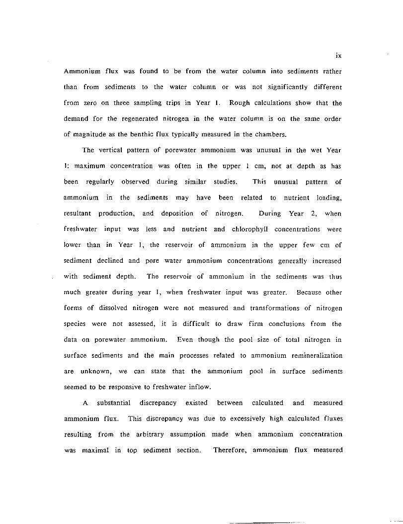
Ammonium flux was found to be from the water column into sediments rather

than from sediments to the water column or was not significantly different

from zero on three sampling trips in Year 1. Rough calculations show that the

demand for the regenerated nitrogen in the water column is on the same order

of magnitude as the benthic flux typically measured in the chambers.

The vertical pattern of porewater ammonium was unusual in the wet Year

I: maximum concentration was often in the upper

been regularly observed during similar studies.

cm, not at depth as has

This unusual pattern of

ammonium In the sediments may have been related to nutrient loading,

resultant production, and deposition of nitrogen. During Year 2, when

freshwater input was less and nutrient and chlorophyll concentrations were

lower than in Year I, the reservoir of ammonium in the upper few cm of

sediment declined and pore water ammonium concentrations generally increased

with sediment depth. The reservoir of ammonium in the sediments was thus

much greater during year I, when freshwater input was greater. Because other

forms of dissolved nitrogen were not measured and transformations of nitrogen

species were not assessed, it is difficult to draw firm conclusions from the

data on porewater ammonium. Even though the pool size of total nitrogen in

surface sediments and the main processes related to ammonium remineralization

are unknown, we can state that the ammonium pool in surface sediments

seemed to be responsive to freshwater inflow.

A substantial discrepancy existed between calculated and measured

ammonium flux. This discrepancy was due to excessively high calculated fluxes

resulting from the arbitrary assumption made when ammonium concentration

was maximal in top sediment section. Therefore, ammonium flux measured

x

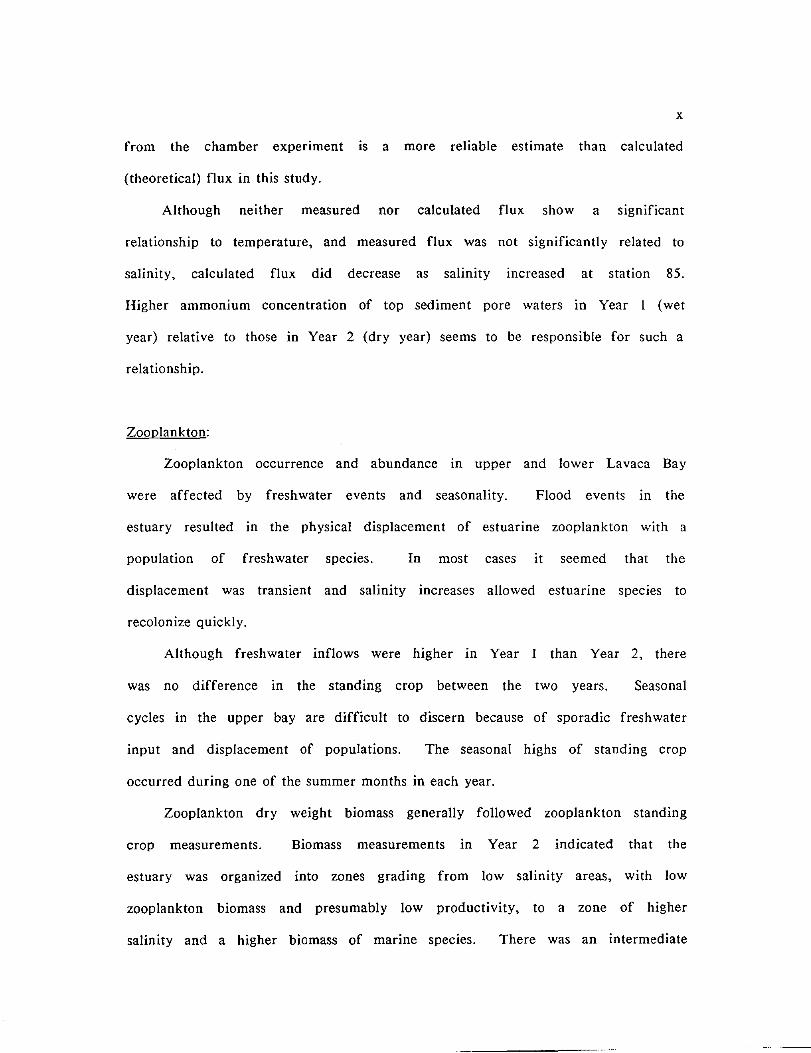
from the chamber experiment is a more reliable estimate than calculated

(theoretical) flux in this study.

Although neither measured nor calculated flux show a significant

relationship to temperature, and measured flux was not significantly related to

salinity, calculated flux did decrease as salinity increased at station 85.

Higher ammonium concentration of top sediment pore waters in Year (wet

year) relative to those in Year 2 (dry year) seems to be responsible for such a

relationship.

Zooplankton:

Zooplankton occurrence and abundance in upper and lower Lavaca Bay

were affected by freshwater events and seasonality. Flood events in the

estuary resulted in the physical displacement of estuarine zooplankton with a

population of freshwater species. In most cases it seemed that the

displacement was transient and salinity increases allowed estuarine species to

recolonize quickly.

Although freshwater inflows were higher in Year I than Year 2, there

was no difference in the standing crop between the two years. Seasonal

cycles in the upper bay are difficult to discern because of sporadic freshwater

input and displacement of populations. The seasonal highs of standing crop

occurred during one of the summer months in each year.

Zooplankton dry weight biomass generally followed zooplankton standing

crop measurements. Biomass measurements in Year 2 indicated that the

estuary was organized into zones grading from low salinity areas, with low

zooplankton biomass and presumably low productivity, to a zone of higher

salinity and a higher biomass of marine species. There was an intermediate

xi

zone where estuarine species predominated. This was also the zone of highest

zooplankton standing crops. This middle-bay region, which moved some with

periodic freshwater events, had relatively stable salinities and represented a

buffer between the low salinity regime and the marine zone. The extent to

which marine species range into the middle and upper bay is dependent on the

salinity gradient established by freshwater inflow. It is concluded that the

distributions of freshwater, estuarine and marine zooplankton species were

quite responsive to physical forcing associated with freshwater input.

The body length of the dominant estuarine zooplankter, Acarlia lOllSa,

was measured systematically. There was a significant positive correlation

between body length and salinity. Two distinctly different populations of this

species may occur in the same estuary or else the size variations are due to

other environmental factors.

this study.

Benthos:

Secondary productivity was not assessed during

Very little change was seen in the concentrations of benthic organisms

between Years I and 2. The vertical distribution of infauna in the sediment

was typical for this type of estuary. Highest concentrations of organisms were

found in the upper 3 cm.

concentrations at 10-20 cm.

Numbers declined with depth to the lowest

Although abundances changed little between years, benthic biomass did

show a pattern, with an overall increase in biomass for Year 2. Biomass,

unlike individual abundance, increased with depth. The largest biomass

measurements were in the 10-20 cm stratum. The molluscs, Mulillia lateralis

Xli

and Macoma mitchelli, had an overwhelming effect on these patterns of benthic

biomass.

Any relationship between freshwater input and benthic biomass will

depend on the nature of the effect (e.g. enhanced survival and growth, or

perhaps restricted recruitment) and the generation times of the benthic

organisms. Influences of freshwater input on recruitment might show up

months later in the biomass of a cohort whereas effects of freshwater inflow

on growth or survival should reflect average conditions over an extended

period, possibly offset by a lag. Simple correlations between infaunal biomass

and short-term stream flow are not to be expected, except in special cases.

The only species which were affected by inflow on a short term were the

aquatic chironomid larva which had a lagged response to inflow and the

polychaete, Hobsonia florida.

Finfish and Shellfish:

The purpose of this component was to provide data on the utilization of

the Lavaca River delta as a nursery habitat for finfish and selected macro­

invertebrates.

As is typical of fish populations, a small number of species comprised the

bulk of the population. The seven most abundant species accounted for 75% of

the total number of individuals collected. Cluster analysis yielded a significant

temporal grouping of three "seasons". These seasonal distribution patterns

were relatively consistent between the two years despite significant differences

in salinity. Spatial patterns were a minor factor in groupings shown by cluster

analysis.

XIII

It is concluded that the primary factor influencing changes in fish species

composition in the Lavaca River delta is the sequential arrival and departure

of postIarval and juvenile fishes and invertebrate species. Salinity effects

were seen only as a minor perturbation within these major temporal patterns.

The data show that the Lavaca River delta is utilized extensively as a

nursery area by most estuarine dependent species which are of commercial or

recreational importance in the Gulf of Mexico. There are also numerous other

species utilizing the delta as a nursery area, many of which are important

components in the food web leading to commercial or recreational species.

The seasonal pattern is, therefore, a reflection of spawning times of

these species utilizing the delta as a nursery. In general, the "seasons"

include the juveniles of winter spawners in March-June and the spring and

early summer spawners in July-October. The low number of species spawning

in late summer are reflected in the relatively low diversity of the November­

February period.

Stable Isotopes:

The objective of the stable isotope studies was to determine the extent

of utilization of river-transported organic matter by the biota of the system.

This was to be accomplished by applying a mixing model to infer carbon

sources based on different .s13C characteristics of organic carbon from maflne

and terrestrial sources. The model indicated that substantial river-transported

C3-higher plant organic carbon is being taken up and assimilated by organisms

in the Lavaca Bay ecosystem. Strong correlations between .sI3C and distance

of collecting station from the river were shown by sedimentary total organic

matter, total infauna, total bivalves and net zooplankton; moderate correlations

XIV

were shown by total fish, total shrimp and Acartia tOl/sa; weak correlations

were shown by dissolved and particulate organic matter.

As might be expected, samples from Matagorda Bay always showed less

higher plant influence than did Lavaca Bay samples. This difference is

probably a good measure of the importance of river transported organic matter.

Fish as a group seemed to be related to phytoplankton in both bays while

shrimp showed a definite river/higher plant signal. Acartia tOl/sa, an estuarine

copepod, reflected a higher plant based food-web, possibly based on a detrital­

microbial pathway.

While 013C data provides no information on the number of animals

utilizing a given source of carbon, when combined with abundance and

distribution data from other studies, it permits an assessment of the relative

importance of organic carbon from different sources. The study area was

found to have diverse food-webs with animals utilizing both the river and bay

as sources of nutrition.

Comments and Conclusions

This was not a process-oriented study but many insights into processes

were obtained. The results of the study have stimulated many suggestions for

future research. Some have been incorporated into a follow-up program in San

Antonio Bay.

A few topics deserve mention. Primary productivity (including

photosynthesis as a function of light) should be measured regularly. A special

effort should be made to assess any physiological differences associated with

salinity and perhaps nutrient input. Primary production by the

microphytobenthos should be assessed as well as the effects of resuspension.

xv

Almost nothing is known of the proximate fate of primary productivity nor the

relative importance of different paths of nutrient regeneration, even though

very close coupling of growth and g-razing of phytoplankton is indicated.

Filter feeding by benthic macrofauna, including patchily-distributed oysters,

might be very important. Further work should be done on methods to measure

fluxes at the sediment-water interface. Rates of nutrient transformations

should be measured as well as pools and fluxes of dissolved organic nitrogen.

Secondary production should be estimated and related to freshwater input via

primary production. Growth rates of fish should be estimated to evalute the

estuary as a nursery.

analytical ambiguity.

Stable isotope studies should use two tracers to reduce

While keeping in mind the large quantity of useful information that was

obtained during this study, it is useful to examine some of the limitations, too.

The sampling scheme that was chosen for this study determined the types of

relationships that could be effectively observed. The temporal scale (i-2

months between samplings) was too coarse to observe the dynamic relationships

between nutrient injections and uptake by phytoplankton. Also, it was not

possible to quantify the importance of sediment resuspension in redistributing

the autotrophic community. Analytical problems plagued measurements of

benthic nutrient regeneration to the extent that modification of sampling

frequency is not a priority. The sampling schedule seemed to be appropriate

for documenting the influence of freshwater, especially flood events, on the

distributions of zooplankton. However, measurements of standing crops of

zooplankton do not convey a compreshensive description of secondary

productivity. Relatively slow-growing benthic infauna were sampled fairly well

(with notable exception of oysters), but the length of the record (2 years) was

XVI

too short to document many possible relationships between freshwater input

and the benthic community. Because mechanisms of freshwater influence are

not specified, it is difficult to know what correlations and what lag periods

should be expected. The sampling frequency was adequate to document the

seasonal utilization of the river delta by fish and it was shown that the

distribution of fish was not very sensitive to changes in salinity. The

importance of freshwater to the estuary as a nursery was not assessed

comprehensively, however, because growth rates and survival were not

determined. Stable isotope studies are inherently immune from some problems

of sampling scales, because the organisms integrate their own environment on

scales appropriate to them. Highly mobile organisms might frustrate some

analyses, because their movements prior to sampling cannot be specified.

One approach to assessing the influence of freshwater on an estuary

would be to obtain a very long time series (20 or more years) of finfish and

shellfish abundance and correlate the data with freshwater inflow and other

pertinent parameters. Analysis might not be straightforward because of

unnatural external influences. Also, the influences of physical forcing would

not be described mechanistically. The data set would be of great value

nonetheless.

Despite some inherent limitations, this study was successful in describing

many responses of an estuarine system to freshwater input.

further study were clearly indicated.

REFERENCES

Directions for

Haury, L.R., J.A. McGowan and P.H. Wiebe. 1979. Patterns and processes in

the time-space scales of plankton distributions.

Spatial Patterns in Plankton Communities. Plenum.

XVII

In: J.H. Steele, (ed.),

Lewis, M.W. and T. Platt. 1982. Scales of variability In estuarine ecosystems.

In: V. Kennedy (ed.), Estuarine Comparisons. Academic.

j

j

j

j

j

j

j

j

j

j

j

j

j

j

j

j

j

j

j

j

j

j

j

j

j

j

I

CHAPTER I

INTRODUCTION

1.1

A two year study to monitor the effects of freshwater inflow on

selected sites in the upper portion of the Lavaca-Tres Palacios Estuary and

parts of Matagorda Bay was conducted from November 1984 through August

1986. Increasing freshwater demands for industry, municipalities, agriculture,

and recreation have made provision of sufficient freshwater inflow to maintain

maximum production in Texas bays and estuaries a major concern. One means

of allocating freshwater among competing users is the construction of dams on

the rivers which supply Texas estuaries; e.g. the Navidad River which was

dammed in May 1980 to form Lake Texana. This reservoir was constructed to

supply water for industrial and municipal use and was not intended for flood

control. Major floods are allowed to pass through the flood gates and

inundate the marsh system associated with the Lavaca-Navidad River delta.

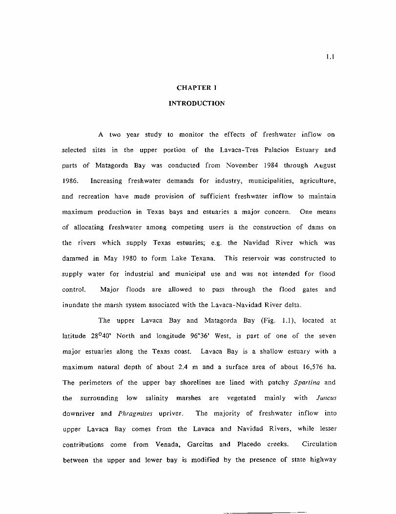
The upper Lavaca Bay and Matagorda Bay (Fig. 1.1), located at

latitude 280 40' North and longitude 96°36' West, is part of one of the seven

major estuaries along the Texas coast. Lavaca Bay is a shallow estuary with a

maximum natural depth of about 2.4 m and a surface area of about 16,576 ha.

The perimeters of the upper bay shorelines are lined with patchy Spartina and

the surrounding low salinity marshes are vegetated mainly with JUilCUS

downriver and Ph rag mites upriver. The majority of freshwater inflow into

upper Lavaca Bay comes from the Lavaca and Navidad Rivers, while lesser

contributions come from Venada, Garcitas and Placedo creeks. Circulation

between the upper and lower bay is modified by the presence of state highway

1.2

35 causeway, the remains of the old causeway, and the presence of

Chickenfoot Reef which extends from the west side of the bay parallel with

the causeway. Marine influence enters through Pass Cavallo and the

Matagorda Ship Channel.

Two small tertiary bays or lakes are associated with the Lavaca

River. Redfish Lake (Station 603) is approximately 4.8 km (3 miles) and Swan

Lake (Station 613) is approximately 1.6 km (1 mile) north of Lavaca Bay (Fig.

1.1). Redfish Lake is about 194 ha (0.75 miles2) and Swan Lake is about 259

ha (I mile2). Both lakes are shallow with a maximum depth of about 1.2 m.

The salinity of Redfish Lake is usually similar to the river's while the salinity

in Swan Lake is more estuarine due to its proximity to and its connection to

Lavaca Bay via Catfish Bayou. Parts of the study area description were

derived from previous work by Gilmore et al., 1976.

Historically, upper Lavaca Bay has been mainly supplied with

freshwater from the Lavaca and Navidad Rivers. The forty-five year daily

flow average for the Lavaca River is 334 cubic feet/second and the forty year

daily flow average for the Navidad River is 572 cubic feet/second (U.S.

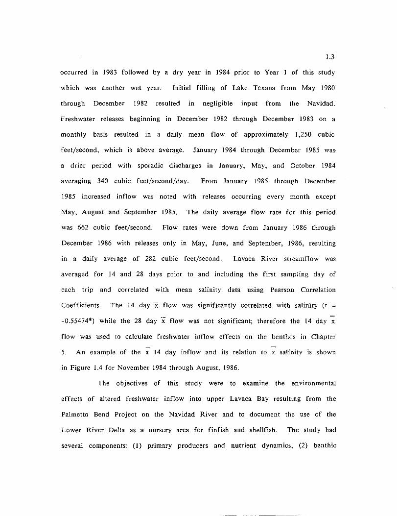
Geological Survey Water Data Report). Daily mean stream flow into Lavaca

Bay from 1975 through 1986 is illustrated in Figure 1.2. Freshwater inflow

rates from gauge 08164000 on the Lavaca River near Edna, Texas indicates that

the average daily flow rate for Year I of this study was 357 cubic feet/second,

50% higher than the daily average of 177 during Year 2. Since the closing of

the dam on the Navidad River in May, 1980 the freshwater inflow pattern has

been altered, although it has not deviated much from the historic flow rate of

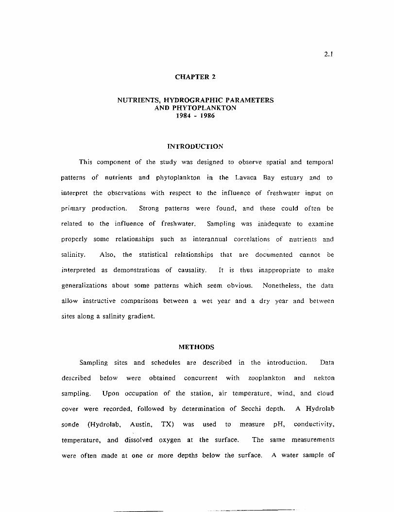
572 cubic feet/second. The average stream flow from January 1983 through

1986 demonstrates cyclic inflow from year to year (Fig. 1.3). A wet cycle

1.3

occurred in 1983 followed by a dry year in 1984 prior to Year 1 of this study

which was another wet year. Initial filling of Lake Texana from May 1980

through December 1982 resulted in negligible input from the Navidad.'

Freshwater releases beginning in December 1982 through December 1983 on a

monthly basis resulted in a daily mean flow of approximately 1,250 cubic

feet/second, which is above average. January 1984 through December 1985 was

a drier period with sporadic discharges in January, May, and October 1984

averaging 340 cubic feet/second/day. From January 1985 through December

1985 increased inflow was noted with releases occurring every month except

May, August and September 1985. The daily average flow rate for this period

was 662 cubic feet/second. Flow rates were down from January 1986 through

December 1986 with releases only in May, June, and September, 1986, resulting

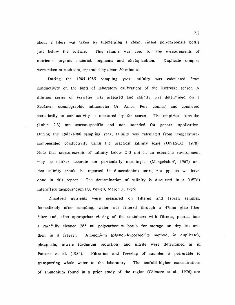
in a daily average of 282 cubic feet/second. Lavaca River streamflow was

averaged for 14 and 28 days prior to and including the first sampling day of

each trip and correlated with mean salinity data using Pearson Correlation

Coefficients. The 14 day x flow was significantly correlated with salinity (r =

-0.55474*) while the 28 day x flow was not significant; therefore the 14 day x

flow was used to calculate freshwater inflow effects on the benthos in Chapter

5. An example of the x 14 day inflow and its relation to x salinity is shown

in Figure 1.4 for November 1984 through August, 1986.

The objectives of this study were to examine the environmental

effects of altered freshwater inflow into upper Lavaca Bay resulting from the

Palmetto Bend Project on the Navidad River and to document the use of the

Lower River Delta as a nursery area for finfish and shellfish. The study had

several components: (1) primary producers and nutrient dynamics, (2) benthic

1.4

nutrient regeneration, (3) zooplankton, (4) benthos, (5) finfish and shellfish

and (6) natural isotopic studies of organic input in Lavaca Bay.

Fourteen sampling trips were conducted which incl~ded the following

months: November 1984, January, March, April, May, June, July, August,

October and December 1985, and February, March, June and August 1986. Year

I of the study was from November 1984 through August 1985 and Year 2 was

from October 1985 through August 1986. Each sampling trip involved two days

in Lavaca Bay. The first day's sampling included zooplankton, ichthyoplankton,

trawls, chemistry, nutrients, hydrographic parameters, and phytoplankton.

Benthic respiration chambers and primary production experiments aboard the

R/V KA TY, benthic cores, seine and sled samples were collected on the second

day. Stations in the lower bay were sampled on the return trip to Port

Aransas aboard the R/V KA TY.

The first eight trips focussed mainly on stations located in the

upper part of the bay north of state highway 35. The sampling sites in Figure

1.1 included stations 45 and 65 (river sites), 603, 613, 623 (lake sites), 85

(river delta) and 633 (upper bay). Two additional stations, 1505 and 1905 were

sampled for nutrients, hydrography, and phytoplankton. Benthic respiration

chambers were deployed only at station 85.

During the last 8 trips stations 1, 2, 3, 1505, 1905 and 35-36 south

of highway 35 were added for zooplankton. Stations 65, 613 and 623 for

isotope analyses were discontinued and stations 1505, 1905 and 35-36 III the

lower bay were added to increase coverage over a greater salinity range.

Support vessels included the R/V KA TY, a 58' fiberglass trawler

which was anchored at station 85 for laboratory space and berthing, a 21' Skip

Jack, and a 16' Boston Whaler.

1.5

ACKNOWLEDGEMENTS

Our appreciation is offered to the following collaborators for their

field sampling efforts, laboratory work up, and cooperation in making this

project successful: Amy Whitney, Hugh McIntyre, Carolyn Miller, Don Pierson,

Zhu Mingyuan and Chris Schneider (Nutrient Dynamics and Primary

production), Judy Lee (Nutrient Regeneration), Lynn Tinnin, Julie Findley and

Wen Lee (Zooplankton and Benthos), Dee Fajardo, Li Maotang, Wen Lee

(Finfish and Shellfish), Richard Anderson and Della Scalan (Isotopes and Marsh

Plant Input), Hayden Abel, Noe Cantu, Don Gibson, John Turany, Billy

Slingerland (Boat Crew), and Helen Garrett (Word Processor Operator). Special

thanks also are due Dr. Ed Buskey, Dr. Paul Montagna and Dr. Terry Whitledge

for technical input and assistance on construction of several of the chapters.

Rob Lane provided a considerable amount of data mangaement for this project.

REFERENCES

Gilmore, G.H., J. Dailey, M. Garcia, N. Hannebaum, J. Means. 1976. A study of

the effects of fresh water on the plankton, benthos, and nekton

assemblages of the Lavaca Bay System, Texas. Tex. Pks. Widlf.·

Dept., Coastal Fish., Div. Tech. Rep. to the Tex. Wat. Dev. Bd., 113

p.

Figure 1.1. l1ap of Lavaca Bay study area. with sample stations indicated.

1.6

MATAGORDA

BAY

f «

o I 234M

c u

f t

p c r

s fl c

':"'llll\ 1

I ,,: 'H)

1 (I)n

1·1, )i)

I; 1)0 /., " .

1 (1110 + / ", ." ,",no i' t:, () (I 0'.---'·,. _,_~~·o'.'"

I ,·1 ~'. • (, U .,/,"""

,,()ol

ut-.. +-I <1-",7C

" '.-' 1'~ 7(,

Average Oal1y Stream Flow into Lavaca Bay

",

'. 0'"

• / \ , \

\ \ ,

, / ~ , ' ,

~~ /

//

,,0

• \

'-

". -' . - 1·- , t·· - .-!-- ..

\ \,

~"1Ir11"tll) C',I;[IIJ

~'r'(Jipct [,);11"11. i l;~(;: 1 .~.) ,:--) (,I

I

0- ~ "'--'" .. '

"~,

\"x \. // \.

• ·,·1 . --·e.>

• .. \ , , i \

I \ ,/ \

; \ i 0 \ / ,", \

/ ,/ \ \ ,I l \ \

,I l '\ / " \ \

,/ /' \ \. ,. / \ \

/ / '. \ • I' \ \

,/ \\ ' , \ / \ \ !

'. I , \. ,'-'--. b /

! o .' +

I 'X/'! .,', I

1 ':f ./ ,~.~ 19 7 \,,~ I')r:',(.l I '·i ;;', 1 I'j?<~' 1 ,~! C' ... ' ~." '-' ,_,I

19:'.,j

• L dV ,'11,:;, I', o I·j;'l',. pJld [, .1 u1:)1

;

~1\11L 1111111'", .J wry' I ',L>!

I i:-,::"t,

•

() \

•

. I

I'·!"',"

, ''''1

l

~

Fig. 1.2. Average daily Lavaca-Navidad River flow into Lavaca Bay by year from 1975 through 1986. ~

5000 c U 4500

f t

4000

3500

3000

P 2500

e 2000 r

s e c

1500

1000

500

o

Average stream flow into Lavaca Bay

Vertical bars i ndic~te 3ampli n'J tt"i ps

Jen 83 Apr 83 Jul 83 Oct 83 Jan 84Apr 84~lul 84 Oct 84 Jan 85 Apr 85 Jul 85 Oct 85 Jan 86Apr 86 Jul 86

I ETI T ot~ 1 llllll r~avi dad R" til Leveca R" I ~

Figure 1.3. Average daily Lavaca-Navidad River flow into Lavaca Bay by month from January 00 1983 through August 1986.

Salinity and Streamflow in Lavaca Bay ppt

20

i8

16

14

12

10

8

6

4

~ j\

I ' I ' . \

I \ I \

/ \ ,. \

/ " I <>-, /0 .'.

// ' / ~ / ''0

//~ ,,' , // \

I~ \

/ \ I ' / '

/ \ / \\

,0------0 \

") L

0 Oct-84 ,Jan-8S Apr-85 Aug- 85 ~lov- e.s Feb-56 r1ay-86

0- ['lean Salinity (ppt) - t'lean Sfreamflow (eLi fUsee) J Figure 1.4. Lavaca River streamflow 14 day average prior to each sampling trip and its

relation to average salinity for all stations by month from November 1984 through August 1986. The 14 day average streamflows corresponding with each sampling trip starting in October 1984 are as follows: 63, 424, 926, 377, 1913, 97, 349, 19, 33, 521, 43, 32, 258, and 15 cu ft/sec.

cu ftl sec

2000

1800

1600

1400

12U)

IOU)

80C

60C

400

20(,

o Sep-56

...... \0

CHAPTER 2

NUTRIENTS, HYDROGRAPHIC PARAMETERS AND PHYTOPLANKTON

1984 - 1986

INTRODUCTION

2.1

This component of the study was designed to observe spatial and temporal

patterns of nutrients and phytoplankton in the Lavaca Bay estuary and to

interpret the observations with respect to the influence of freshwater input on

primary production. Strong patterns were found, and these could often be

related to the influence of freshwater. Sampling was inadequate to examine

properly some relationships such as interannual correlations of nutrients and

salinity. Also, the statistical relationships that are documented cannot be

interpreted as demonstrations of causality. It is thus inappropriate to make

generalizations about some patterns which seem obvious. Nonetheless, the data

allow instructive comparisons between a wet year and a dry year and between

sites along a salinity gradient.

METHODS

Sampling sites and schedules are described in the introduction. Data

described below were obtained concurrent with zooplankton and nekton

sampling. Upon occupation of the station, air temperature, wind, and cloud

cover were recorded, followed by determination of Secchi depth. A Hydrolab

sonde (Hydrolab, Austin, TX) was used to measure pH, conductivity,

temperature, and dissolved oxygen at the surface. The same measurements

were often made at one or more depths below the surface. A water sample of

2.2

about 2 liters was taken by submerging a clean, rinsed polycarbonate bottle

just below the surface. This sample was used for the measurements of

nutrients, organic material, pigments and phytoplankton.

were taken at each site, separated by about 20 minutes.

Duplicate samples

During the 1984-1985 sampling year, salinity was calculated from

conductivity on the basis of laboratory calibrations of the Hydrolab sensor. A

dilution series of seawater was prepared and salinity was determined on a

Beckman oceanographic salinometer (A. Amos, Pers. comm.) and compared

statistically to conductivity as measured by the sensor. The empirical formulas

(Table 2.3) are sensor-specific and not intended for general application.

During the 1985-1986 sampling year, salinity was calculated from temperature­

compensated conductivity using the practical salinity scale (UNESCO, 1978).

Note that measurements of salinity below 2-3 ppt in an estuarine environment

may be neither accurate nor particularly meaningful (Mangelsdorf, 1967) and

that salinity should be reported in dimensionless units, not ppt as we have

done in this report. The determination of salinity is discussed in a TWDB

interoffice memorandum (G. Powell, March 3, 1986).

Dissolved nutrients were measured on filtered and frozen samples.

Immediately after sampling, water was filtered through a 47mm glass-fiber

filter and, after appropriate rinsing of the containers with filtrate, poured into

a carefully cleaned 265 ml polycarbonate bottle for storage on dry ice and

then in a freezer. Ammonium (phenol-hypochlorite method, in duplicate),

phosphate, nitrate (cadmium reduction) and nitrite were determined as in

Parsons et al. (1984). Filtration and freezing of samples is preferable to

transporting whole water to the laboratory. The tenfold-higher concentrations

of ammonium found in a prior study of the region (Gilmore et aI., 1976) are

2.3

thus possibly attributed to artifact. Our method of filtering and freezing prior

to analysis is better than those used previously but they are not optimal: it is

generally held that ammonium measurements on frozen samples are unreliable

and that only fresh samples can be used for critical measurements of

ammonium concentration. Uncertainty associated with freezing may be on the

order of .5 ug-at/l (.007 mg/l Nil), not much of a problem in the context of

this study.

Total Kjeldahl Nitrogen was determined by W. M. Pulich, Jr. on whole­

water samples poisoned with HgCl2 and stored at 20 C. Total phosphate

(persulfate digestion in an autoclave) was measured, usually in triplicate, on

whole-water samples stored at 20 C' For unknown reasons our measurements of

total phosphate tend to be about twice as high as those reported by Gilmore

et al. (1976) for the Lavaca Bay region in 1973-1975.

Samples were collected on What man GF/F filters (0.7um nominal

retention) and extracted in 90% acetone for duplicate fIuorometric

determinations of chlorophyll l! and pheopigment (Parsons et aI., 1984). Values

for chlorophyll and pheopigment from the progress report for 1984-85 have

been corrected for a calibration error. Pheopigments are reported in J.Lgr l

chlorophyll equivalents. Because of interference from pigments such as

chlorophyll 12 (Lorenzen and Jeffreys, 1980) and problems associated with

incomplete extraction of some taxonomic forms in acetone (Holm-Hansen and

Riemann 1978), pigment data should be viewed with some caution. When

comparing these pigment data with other studies, pore size of filters should be

noted, as significant proportions of phytoplankton biomass can pass filters of I

urn pore size and larger.

2.4

Samples for phytoplankton enumeration were preserved with Lugol's

solution and settled for observation with an inverted microscope at lOOx and

400x magnification. Representative cell dimensions for each common form was

recorded and biovolume calculated by geometrical approximation. Cell counts

reported here are higher than what might be found in earlier studies because

the abundant and very small «Sum) forms were counted. There is a systematic

difference between the counts for Year and Year 2 attributable to

differences in the counts for extremely small phytoplankton. Th is is because

the two operators had different "thresholds" for counting the smallest cells.

Therefore the two years cannot be legitimately compared for total cell counts

or biovolume. Although many small phytoplankton can be discerned with the

inverted microscope, a technique such as epifiuorescence microscopy is needed

for accurate assessment of autotrophs in the O.Sum-2um· range (Johnson and

Sieburth 1979). Methods used in this study have probably yielded

underestimates of the smallest phytoplankton in Year 2 as well as in Year I,

even though some heterotrophic bacteria may have unavoidably been confused

with cyanobacteria in the counts from Year 2.

The data were subjected to a variety of statistical analyses, including

linear regression, one- and two-way analysis of variance (parametric and

nonparametric), non parametric

Whitney U test. Missing

correlation, Tukey's HSD test, and the Mann­

values and violations of the assumptions of

parametric statistics plagued the analysis, and thus the statistical presentation

is limited. The results presented here were generated by SYST A T for the

Macintosh (Wilkinson, 1986), except the regressions, which were generated by

Cricket Graph.

2.5

Field sampling was performed by Amy G. Whitney, Hugh MacIntyre, and

Sung R. Yang. Ancillary experimental work was carried out by Zhu Mingyuan

and Richard Davis. Don Pierson and Zhu Mingyuan supervised analytical work

early in the study. Enumeration of phytoplankton was done by Amy Whitney

in Year I and Barbara Cullen in Year 2.

RESULTS

Annual Pattern

A graphic presentation of the data demonstrates very clearly the

dominant patterns during the study. Year I (1984-1985) was relatively wet and

Year 2 (1985-1986) was relatively dry. A salinity gradient, associated with

proximity to freshwater input, was evident throughout the study period (Fig.

2.2). Nitrate concentration (Fig. 2.8) seemed to reflect the importance of

freshwater input to nutrient dynamics. High concentrations were associated

with low salinities and concentrations were very low in the dry year, and at

the bay stations as compared to the upriver stations. The general picture is

one of freshwater input having a very important influence on nutrient

concentrations. A more detailed examination of the data provides additional

insight and some information on biological utilization of the nutrients

associated with freshwater input.

To examine the relationships between freshwater input, nutrient dynamics

and primary production on a scale appropriate to fisheries, it would be useful

to compile a long record and correlate annual averages of salinity, nutrient

concentrations and biological responses. We only have two years to work

with, one wet and one dry, we cannot confidently ascribe statistically

significant differences between years to freshwater influence.

compare the two years nonetheless.

It is useful to

2.6

Stations 1505 and 1905 were least influenced by freshwater and most

afflicted with missing values, they were excluded from the statistical

comparison of Year 1 vs Year 2 (Mann-Whitney U test, Table 2.1). Comparison

of the parameters from the remaining stations (Table 2.1) showed substantial

differences between years that are in most cases evident in graphical

presentation (Figs. 2.1-2.13). The water was indeed fresher in Year I (p<.OO I)

and the concentrations of dissolved nutrients, excluding ammonium, were

substantially higher in the wet year (p<.OOI), as was total phosphate. Pigment

concentrations were significantly higher in the first year, consistent with, but

not demonstrating, higher primary production. Total Kjeldahl nitrogen (TKN)

did not behave the same as other measures of nutrient loading: concentrations

were higher in the second year. Nitrate and nitrite are not measured by the

Kjeldahl method. Total nitrogen, here defined as TKN + nitrate + nitrite, was

not significantly different between years.

are discussed below.

Nitrogen and phosphorus dynamics

It is reasonable to expect that enhanced flushing associated with

freshwater input would increase turbidity due to sediment resuspension and

transport. The relationship was obvious to the sampling party and is

represented by the differences in Secchi depth between Year I and Year 2

(Fig. 2.5). If phytoplankton biomass is held steady or is flushed away,

increased turbidity from freshwater input will reduce water-column primary

productivity. If the nutrient load associated with the freshwater input (Figs.

2.18, 2.19) is converted to biomass, though, productivity on an areal basis will

depend on the relationship between turbidity and nutrient load. If physical

forcing is reduced, particulates can settle out of the water, leaving dissolved

nutrients in a more transparent water column and setting the stage for

2.7

enhanced primary productivity. A comprehensive model of light-nutrient

relationships is beyond the scope of this study.

of productivity are briefly discussed below.

Light and nutrient limitation

Seasonal Pattern

The most obvious seasonal pattern was in temperature (Fig. 2.1), which is

certain to influence rates of biological utilization. Many of the other

measured parameters showed significant variation between months (i.e. sampling

periods; Table 2.2), but simple seasonal variation is difficult to discern, in

large part because inferred freshwater input did not show a simple annual

cycle.

For example, freshwater events in November 1984 and July 1985 were

scarcely noticeable in the record of nitrate concentration (Figs. 2.2, 2.8),

whereas similar patterns of salinity were associated with relatively high

concentrations of nitrate during the spring of 1985 and December 1985.

Temperature alone cannot explain the contrast, as waters were cool (about

15°C) in November 1984 and near 300e in July 1985. Perhaps biological

demand for nutrients builds up during the summer and fall and declines sharply

in the winter. Measurements of chlorophyll are consistent with such an

explanation. In November 1984 and July 1985, chlorophyll concentrations were

higher upriver (Fig. 2.12), indicating that biological utilization of freshwater-

associated nutrients had occurred. When high nitrate concentrations were

observed in low-salinity water during the spring of 1985, chlorophyll was more

concentrated downriver, indicating that flushing of the bay system can force a

temporal and spatial separation of nutrient input and biological utilization.

Such a simple explanation cannot be supported by the data on hand because we

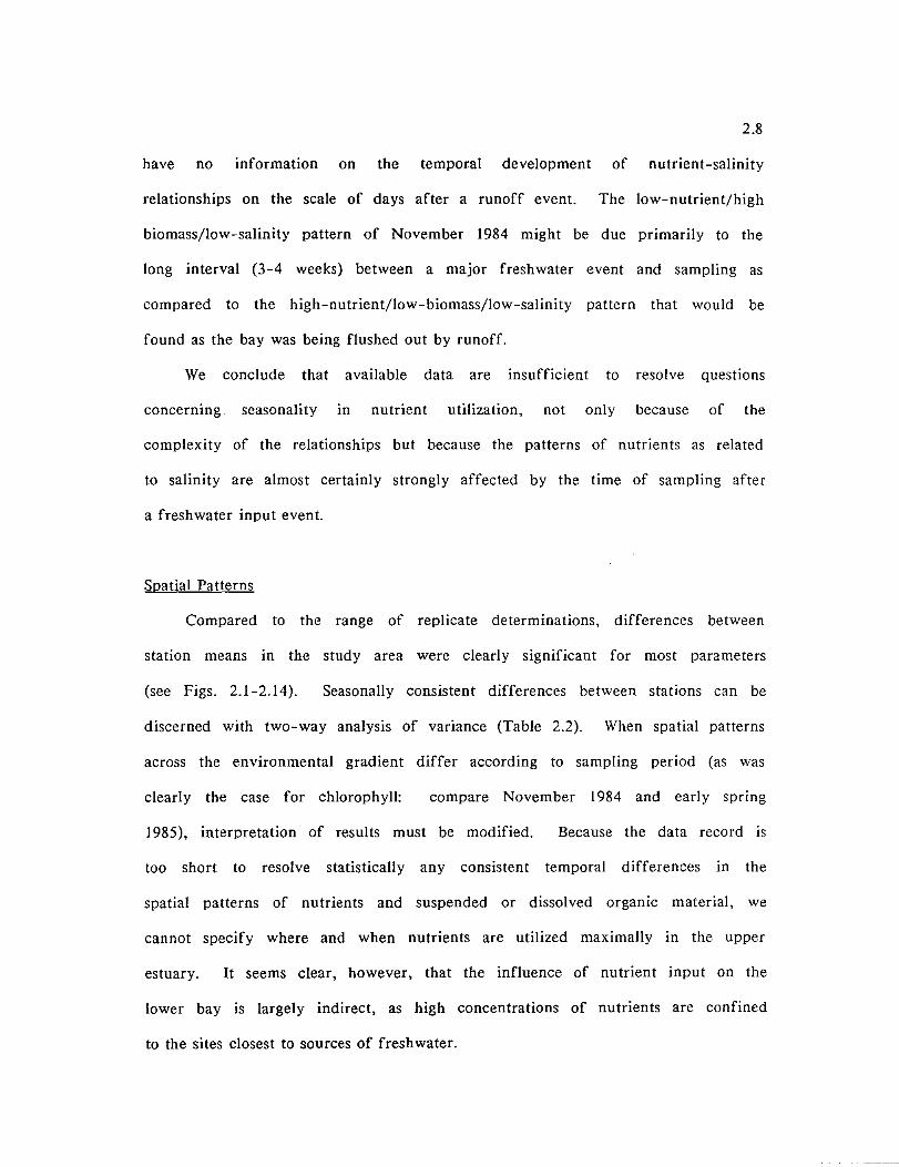
2.8

have no information on the temporal development of nutrient-salinity

relationships on the scale of days after a runoff event. The [ow-nutrient/high

biomass/low-salinity pattern of November 1984 might be due primarily to the

long interval (3-4 weeks) between a major freshwater event and sampling as

compared to the high-nutrient/[ow-biomass/[ow-sa[inity pattern that would be

found as the bay was being flushed out by runoff.

We conclude that available data are insufficient to resolve Questions

concerning seasonality 10 nutrient utilization, not only because of the

complexity of the relationships but because the patterns of nutrients as related

to salinity are almost certainly strongly affected by the time of sampling after

a freshwater input event.

Spatial Patterns

Compared to the range of replicate determinations, differences between

station means in the study area were clearly significant for most parameters

(see Figs. 2.1-2.14). Seasonally consistent differences between stations can be

discerned with two-way analysis of variance (Tab[e 2.2). When spatial patterns

across the environmental gradient differ according to sampling period (as was

clearly the case for chlorophyll: compare November 1984 and early spring

1985), interpretation of results must be modified. Because the data record is

too short to resolve statistically any consistent temporal differences in the

spatial patterns of nutrients and suspended or dissolved organic material, we

cannot specify where and when nutrients are utilized maximally in the upper

estuary. It seems clear, however, that the influence of nutrient input on the

[ower bay is largely indirect, as high concentrations of nutrients are confined

to the sites closest to sources of freshwater.

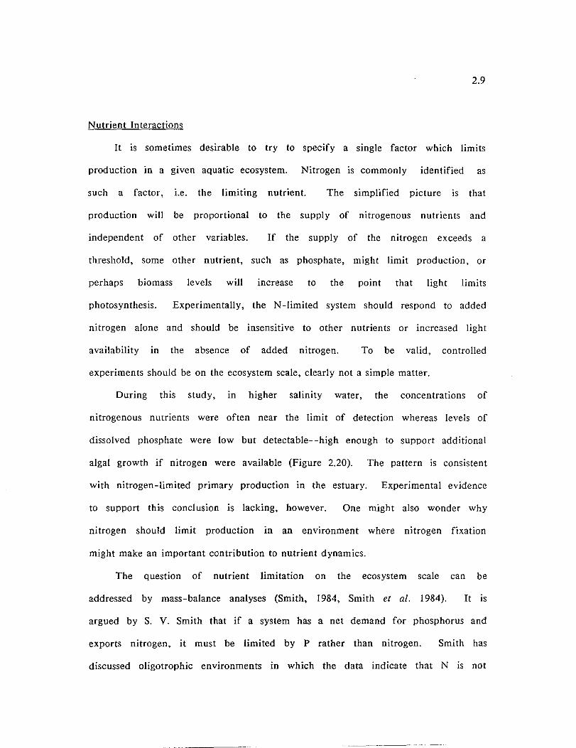
2.9

Nutrient Interactions

It is sometimes desirable to try to specify a single factor which limits

production in a given aquatic ecosystem. Nitrogen is commonly identified as

such a factor, I.e. the limiting nutrient. The simplified picture is that

production will be proportional to the supply of nitrogenous nutrients and

independent of other variables. If the supply of the nitrogen exceeds a

threshold, some other nutrient, such as phosphate, might limit production, or

perhaps biomass levels will increase to the point that light limits

photosynthesis. Experimentally, the N-limited system should respond to added

nitrogen alone and should be insensitive to other nutrients or increased light

availability in the absence of added nitrogen. To be valid, controlled

experiments should be on the ecosystem scale, clearly not a simple matter.

During this study, in higher salinity water, the concentrations of

nitrogenous nutrients were often near the limit of detection whereas levels of

dissolved phosphate were low but detectable--high enough to support additional

algal growth if nitrogen were available (Figure 2.20). The pattern is consistent

with nitrogen-limited primary production in the estuary. Experimental evidence

to support this conclusion is lacking, however. One might also wonder why

nitrogen should limit production in an environment where nitrogen fixation

might make an important contribution to nutrient dynamics.

The question of nutrient limitation on the ecosystem scale can be

addressed by mass-balance analyses (Smith, 1984, Smith et al. 1984). It is

argued by S. V. Smith that if a system has a net demand for phosphorus and

exports nitrogen, it must be limited by P rather than nitrogen. Smith has

discussed oligotrophic environments in which the data indicate that N is not

2.10

limiting. The nature of the Lavaca Bay estuary is such that the assumptions

of the mass-balance analysis are not satisfied (see Smith, 1984), but it is

instructive nonetheless to discuss patterns of Nand P during the study.

Dissolved phosphate, nitrate, and total P concentrations were lower in the

dry year and in higher-salinity water, consistent with biological utilization of

Nand P and net deposition of P in the estuary (Figs. 2.20, 2.21). Total

Kjeldahl nitrogen (organic N and ammonium) weakly shows an inverse pattern,

apparently reflecting the conversion of nitrate to organic nitrogen and little or

no net deposition of N in the study area. Accordingly, total N (nitrite +

nitrate + TKN) shows no consistent relationship with freshwater but the ratio

(Total P ITotal N) declines rather sharply with salinity (Fig. 2.21). Little is

known as to what determines the chemical composition of the salty end­

member of the estuarine water, so non-conservative behavior of phosphorus has

been clearly demonstrated. Thus, the patterns of Nand P observed during this

study do not justify any firm generalizations. Nonetheless, the apparent

relationship between the two nutrients is provocative. It can be inferred from

the relationship between Nand P that any losses of N associated with the loss

of P to the system (i.e. by deposition of organic material) are more than

compensated by processes which act on N but not P, for example nitrogen

fixation. The relatively high concentration of TKN in the dry second year is

consistent with this scenario.

Denitrification can be an important loss term in the estuarine nitrogen

cycle. At the Lavaca Bay study site, denitrification as well as organic

deposition was apparently compensated.

A net demand for P in a system does not demonstrate P limitation.

Nitrogen may limit primary production proximately, but phosphorus input, if

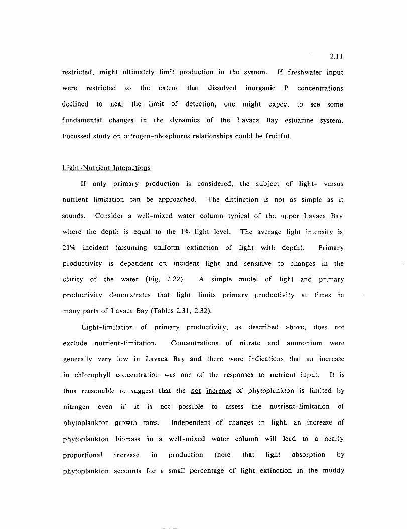
2.11

restricted, might ultimately limit production in the system. If freshwater input

were restricted to the extent that dissolved inorganic P concentrations

declined to near the limit of detection, one might expect to see some

fundamental changes in the dynamics of the Lavaca Bay estuarine system.

Focussed study on nitrogen-phosphorus relationships could be fruitful.

Light-Nutrient Interactions

If only primary production IS considered, the subject of light- versus

nutrient limitation can be approached. The distinction is not as simple as it

sounds. Consider a well-mixed water column typical of the upper Lavaca Bay

where the depth is equal to the I % light level. The average light intensity is

21 % incident (assuming uniform extinction of light with depth). Primary

productivity is dependent on incident light and sensitive to changes in the

clarity of the water (Fig. 2.22). A simple model of light and primary

productivity demonstrates that light limits primary productivity at times in

many parts of Lavaca Bay (Tables 2.31, 2.32).

Light-limitation of primary productivity, as described above, does not

exclude nutrient-limitation. Concentrations of nitrate and ammonium were

generally very low in Lavaca Bay and there were indications that an increase

in chlorophyll concentration was one of the responses to nutrient input. It is

thus reasonable to suggest that the net increase of phytoplankton is limited by

nitrogen even if it is not possible to assess the nutrient-limitation of

phytoplankton growth rates. Independent of changes in light, an increase of

phytoplankton biomass in a well-mixed water column will lead to a nearly

proportional increase in production (note that light absorption by

phytoplankton accounts for a small percentage of light extinction in the muddy

2.12

waters of Lavaca Bay). Primary productivity can thus be limited by light and

nutrients.

Phytoplankton

The quantitative importance of very small phytoplankton in marine and

estuarine systems has only recently been fully appreciated due to the advent of

epifluorescence microscopy (Johnson and Sieburth 1979; Krempin and Sullivan

1981 ). Because epifluorescence microscopy was not employed in this and in

previous studies of Texas bays, the phytoplankton assemblages have not been

fully described. It is thus not surprising that relationships between chlorophyll

and phytoplankton abundance were not clear: correlations between cell counts

and chlorophyll were poor in both years as were the correlations between

biovolume and chlorophyll. Cell counts were a poor estimator of phytoplankton

biomass because cell size is not considered. We suspect that the poor

relationship between biovolume and chlorophyll is due in large part to

uncertainty in counting and sizing the smallest phytoplankton and also in the

highly variable chlorophyll content of microalgae (Cullen 1982). The cell

counts and biovolume estimates from this study are rather poor indicators of

phytoplankton biomass. The counts do show that small forms are important

and do contain a substantial amount of information on relative abundance of

identifiable taxa during the course of the study. An overview of the

taxonomic trends (Figs. 2.16, 2.17; Table 2.30) demonstrates that cyanobacteria

dominated the autotrophic community. Small coccoid cyanobacteria, solitary and

in small colonies, were by far the most abundant. Clearly, more appropriate

methods should be employed to look at the autorophs In this estuarine

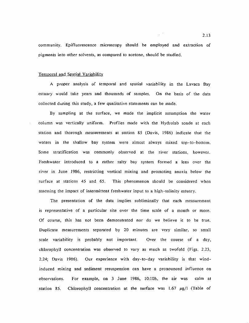
2.13

community. Epifluorescence microscopy should be employed and extraction of

pigments into other solvents, as compared to acetone, should be studied.

Temporal and Spatial Variability

A proper analysis of temporal and spatial variability in the Lavaca Bay

estuary would take years and thousands of samples. On the basis of the data

collected during this study, a few qualitative statements can be made.

By sampling at the surface, we made the implicit assumption the water

column was vertically uniform. Profiles made with the Hydrolab sonde at each

station and thorough measurements at station 85 (Davis, 1986) indicate that the

waters in the shallow bay system were almost always mixed top-to-bottom.

Some stratification was commonly observed at the river stations, however.

Freshwater introduced to a rather salty bay system formed a lens over the

river in June 1986, restricting vertical mixing and promoting anoxia below the

surface at stations 45 and 65. This phenomenon should be considered when

assessing the impact of intermittent freshwater input to a high-salinity estuary.

The presentation of the data implies subliminally that each measurement

is representative of a particular site over the time scale of a month or more.

Of course, this has not been demonstrated nor do we believe it to be true.

Duplicate measurements separated by 20 minutes are very similar, so small

scale variability is probably not important. Over the course of a day,

chlorophyll concentration was observed to vary as much as twofold (Figs. 2.23,

2.24; Davis 1986). Our experience with day-to-day variability is that wind-

induced mixing and sediment resuspension can have a pronounced influence on

observations.

station 85.

For example, on 3 June 1986, 10:IOh, the air was calm at

Chlorophyll concentration at the surface was 1.67 Ilg/1 (Table of

Chlorophyll values).

2.14

The wind was blowing on the next day and the

concentration of chlorophyll at the surface ranged from about II to 15 fLg/1

over the day (Davis, 1986; Fig. 2.24).

Primary Productivity

This study was constrained to measure concentrations of organisms and

materials rather than rate processes such as primary productivity. Only with a

systematic program of rate measurements would it be possible to assess

directly the influences of freshwater input on primary productivity. Even with

a good understanding of that link, it would be difficult to describe

mechanistically the ultimate effects of freshwater input on higher trophic

levels.

Several experiments were performed at station 85 to examine processes

associated with primary production. Some results have been presented (Davis,

1986) but the analysis is not complete. In the results that we have considered

to date (e.g. Fig. 2.25, Table 2.33), photosynthetic rates normalized to

chlorophyll compared favorably to healthy cultures. We have seen no other

indication of severe nutrient limitation of photosynthesis by microalgae.

Studies of benthic and water-column primary productivity are presently

underway in the San Antonio Bay estuary.

The biomass of the microphytobenthos is substantial and distributed well

below the upper millimeter of sediment where net photosynthesis is possible

(H.L. MacIntyre, unpubl.). This algal biomass appears to act as a reservoir of

photoautotrophic potential capable of significant primary production during

resuspension. The seasonal pattern of benthic pigments at two stations is

presented in Fig. 2.26 (H.L. MacIntyre, in prep.). The amount of pigment in

2.15

the upper 5 mm of sediment is on the same order as that suspended in the

water column. Novel measurements of photosynthesis vs irradiance on benthic

samples have demonstrated that the benthic pigments are photosynthetically

active (Fig. 2.27). The effects of sediment resuspension and the associated

inoculum of autotrophs on water-column primary productivity are currently

being studied as part of a research program in the San Antonio Bay.

CONCLUSIONS

Measurements of salinity showed that the Lavaca Bay estuary was

influenced by freshwater. High nutrient concentrations were associated with

freshwater input and biological utilization of the nutrients was indicated by

nutrient depletion away from the input and in the dry year as compared to the

wet year. The flushing action of freshwater inflow was evident during

sampling periods when nutrients were high and chlorophyll was relatively low

in low-salinity water. Our results are consistent with the notion that as flow

subsides, nutrients are utilized and phototrophic biomass increases in the

fresher water. Thus, there is no reason to expect stable relationships between

salinity, nutrients and phytoplankton in an estuarine system subject to episodic

perturbations, at least on the time scale of those perturbations. Over months

or years though, freshwater input nutrients and primary production are likely

to be related. The differences between a wet year and a dry year at Lavaca

Bay are consistent with the proposition that freshwater input has a strong

influence on primary production.

proven, however.

The relationship has by no means been

The ratio of phosphorus to nitrogen in the water column declined as a

function of salinity. There is a large amount of scatter in the data, but it

2.16

appears that phosphorus declined more sharply than would be predicted from

mixing of different water types (i.e. P was removed from the water column)

whereas there was no indication of a net demand for nitrogen. Even though

inorganic nitrogen levels were often very low and the potential for

phytoplankton growth may have been limited by the supply of nitrogen, it is

possible that the supply of phosphorus could ultimately exert an important

control on productivity of the system.

relationships is clearly warranted.

More study on nitrogen-phosphorus

- -----------

2.17

REFERENCES

Cullen, J.J. 1982. The deep chlorophyll maximum: comparing vertical profiles of

chlorophyll a. Can. J. Fish. Aquat. Sci. 39:791-803.

Davis, Richard F. 1986. Measurement of primary production in turbid waters.

M.A. Thesis. University of Texas at Austin.

Gilmore, G., J. Dailey, M. Garcia, N. Hannebaum and J. Means. 1976. A study

of the effects of freshwater on the plankton, benthos, and nekton

assemblages of the Lavaca Bay System, Texas.

Texas Water Development Board. 113 pp.

Harris, G.P., G.D.Haffner and B.B. Piccinin. 1980.

Technical Report to the

Physical variability and

phytoplankton communities: II. Primary productivity by phytoplankton in

a physically variable environment. Arch. Hydrobiol. 88:393-425.

Holm-Hansen, O. and B. Riemann. 1978. Chlorophyll a determination:

improvements in methodology. Oikos 30:438-447.

Krempin, D.W. and C.W. Sullivan. 1981. The seasonal abundance, vertical

distribution, and relative microbial biomass of chroococcoid cyanobacteria

at a station in southern California coastal waters. Can. J. Microbiol.

27: 1341-1344.

Lorenzen, C.J. and S.W. Jeffrey. 1980. Determination of chlorophyll in

seawater. Unesco tech. papers in Mar. Sci. 35. 20 pp.

Mangelsdorf, P.C. Jr. 1967. Salinity measurements in estuaries. In: G.H. Lauff

(ed.), Estuaries. Publ. No. 83, Amer. Assoc. Adv. Sci., Wash. D.C. pp. 71-

79.

Parsons, T.R., Y. Maita and C.M. Lalli. 1984. A manual of chemical and

biological methods for seawater analysis. Pergamon.

2.18

Smith, S.V. 1984. Phosphorus versus nitrogen limitation In the marine

environment. Limnol. Oceanogr. 29:1149-1160.

Smith, S.V., W.J. Kimmerer and T.W. Walsh. 1986. Vertical flux and

biogeochemical turnover regulate nutrient limitation of net organic

production in the North Pacific Gyre. Limnol. Oceanogr. 31:161-167.

Unesco. 1978. Background papers and supporting data on the practical salinity

scale 1978. Unesco tech. papers in Mar. Sci. 37.

Wilkinson, L. 1986. SYSTAT: The System for Statistics. Evanston, IL:

SYSTAT, Inc.

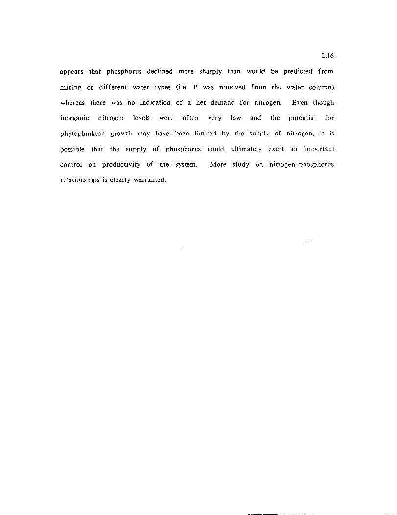
Figure 2.1.

2.19

Temperature measurements made during the Lavaca Bay study,

1984-86. Error bars represent range of duplicate samples taken

about 20 minutes apart. Hydrographic parameters were not

determined in duplicate during the first year.

Temperature 1984 - 1985

40 rj------------------------------------------------------------------------------------------~

30 l- n ~ flh~_ I. 45 II 603 III 65

Col 20 ~ It] swtl 1111 _I _Ii~ lEI I [l 613

• o 623 • 633 e 85 IliiI 1505

10 ~A I=rl ""'-J -=:I:,IA _A _,VI __ A-= -..J1III::t -.-:I l1l:::I:'1' 1 __ ....... 1 [;3 1905

o Nov (Dec) Jan Mar Apr May Jun Jui Aug

Month

Temperature 1985 - 1986

40 r'-----------------------------------------------------------------------------------,

Figure 2.2. Salinity measurements made during the Lavaca Bay study, 1984-

1986. Error bars represent range of duplicate samples taken

about 20 minutes apart. Hydrographic parameters were not

determined in duplicate during the first year.

2.21

..... ... • • ..... • ... 'I -i

..... 1. • ..... • ... '; ... i

Sal1n1ty 1984 - 1985 30i~--------------------------------------------------------------------'

20

10 rI I • JI o

Nov (Dec) Jan Mar Apr May Jun Jul Aug

Month

Sal1n1ty 1985 - 1986

30~i ----~------------------------------------------------------------_.

20

10

o October December February (Mar) April

Month

(May) June a llindl

(Jul) August

.45 II 603 II 65 ~ 613 o 623 • 85 EI 1505 m 1905

.45

.. 603 II 65 f:i::I 613 o 623 • 633 EI 85 [] 1505 12 1905

N . N N

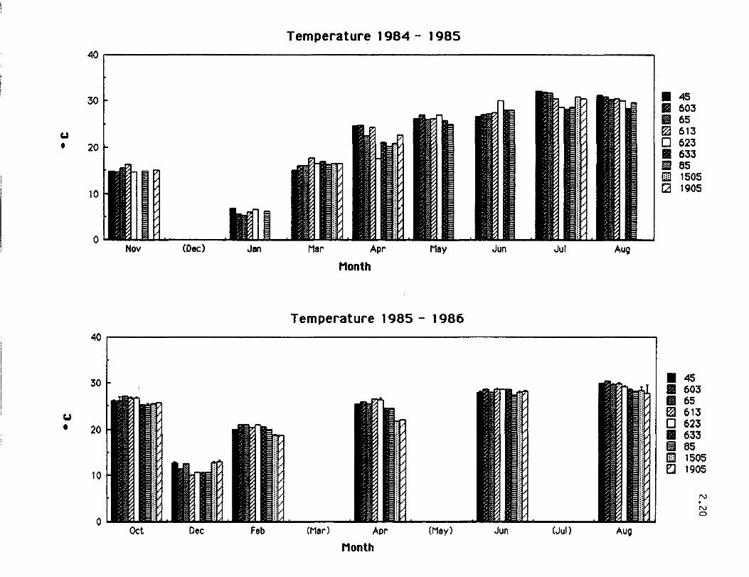
Figure 2.3. pH measurements made during the Lavaca Bay study, 1984-1986.

Error bars represent range of duplicate samples taken about 20

minutes apart. Hydrographic parameters were not determined

in duplicate during the first year.

2.23

pH 1984 - 1985 10ir-------------------------------------------------------------------------~

9, "" '.45 II 603 II 65

z: 8~I~n .~ m '-:1 L .I] Jl:n nl~ Illfflm I ~ 613

• j~ o 623

• 633 8 65 Iilll 1505

7 '--1'A 1 EI L-1 _:~ 113 _::;I 1113:1.-1 -.;! B;!;I:L1 • a:~ B3 ~-=:I _:~ -=:I 1 I2J 1905

6 Nov (Dec) Jan Mar Apr May Jun Jul Aug

Month

pH 1985 - 1986 10~, ----------------------------------------------------------------------------~

9 t-• 45 III 603 IIJ 65

z: 8~.~:f1.IUj •• JJ BrWIH1 • rrIta ~ I ~ 613 o 623 •

• 633 I:iilI 65 [I 1505

7 ~ lI~n1 B[~ 1I!1iI'] ~ Bil] EF..1BiW] ~Bi311 ~EI I [21 1905

N . N

6' .. , Dfff' .. ' , .... , M5fO[" Q =a "'" Oct Dec Feb (Mar) Apr (May) Jun (Jul) Aug

Month

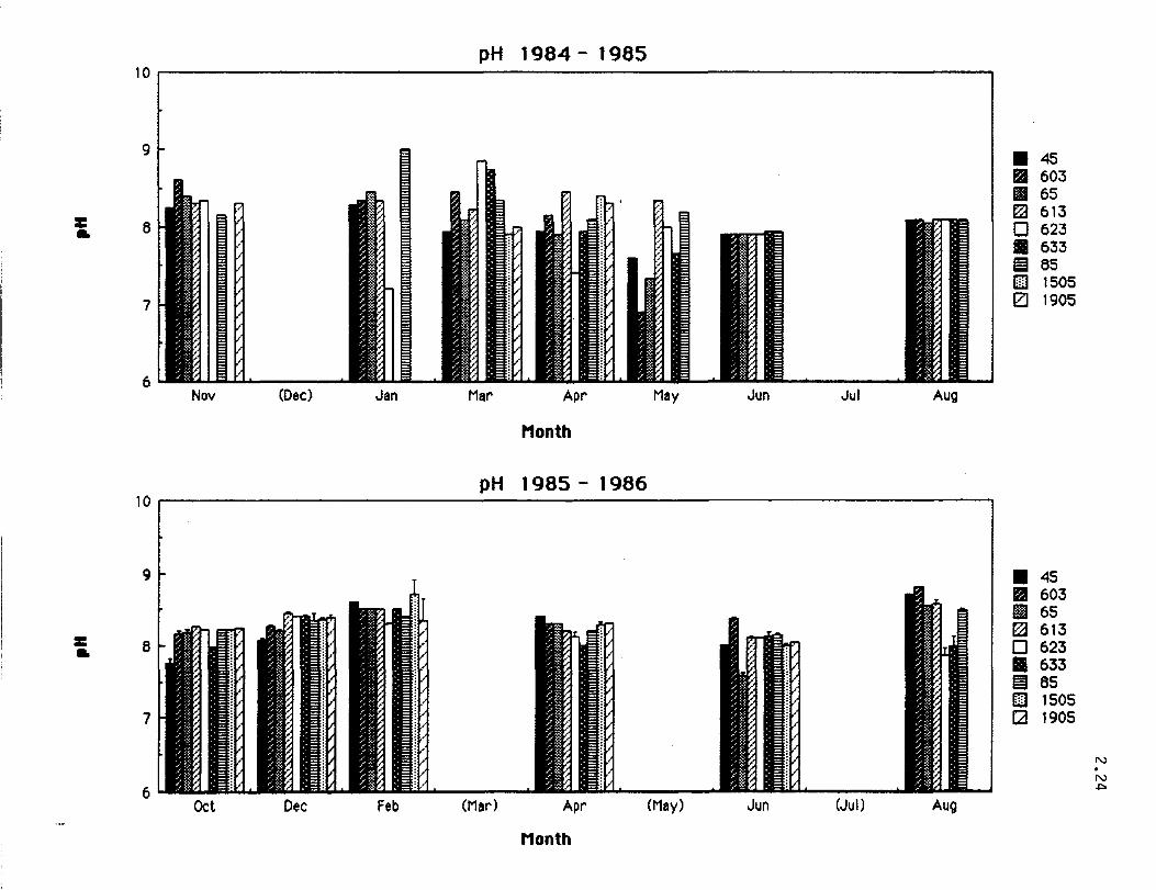
Figure 2.4. Dissolved oxygen measurements made during the Lavaca Bay

study, 1984-1986. Error bars represent range of duplicate

samples taken about 20 minutes apart. Hydrographic parameters

were not determined in duplicate during the first year.

2.25

c:: r

c::: r

D1sso1ved Oxygen 1984 - 1985 20ri--------------------------~~------------------------------~

15 t- t;::Il~

10 ~.a.nI3R III 5~I~n _JI~

o Nov (Dec) Jan

JL RlIIH1

Mar

-- ~-Bt-IIIUi

Apr

Month

I

11 _1:1 1- _t'-'l

mlll:! EJ;I~ B3lili[l ~1IiI

May Jun Jul Aug

D1sso1ved Oxygen 1985 - 1986 15ri----------------------------~--------------------------------~

10 1-.dTh Mlillm .- rJ

~IIB III~ II~ •• Its hi 5 I-IB3IJIl ~lftin Bf:IIiiIJl lIIm.n1 m1l1lf..f lim IIUl I

0 1 I-~ BiE;I;;J "I"~.t iI-";°11 :;a _or, I

Oct Dec Feb (Mar) Apr (May) Jun (Jut) Aug Month

.45 II 603 II 65 ~ 613 o 623 • 633 51 85 [) 1505 !2l 1905

.45 II 603 II 65 ~ 613 o 623 • 633 51 85 [) 1505 EJ 1905

N . N

'"

2.27

Figure 2.5. Secchi depth measurements made during the Lavaca Bay study,

1984-1986. Error bars represent range of duplicate samples

taken about 20 minutes apart. Hydrographic parameters were

not determined in duplicate during the first year.

100

60

60

I u

40

20

0 Nov (Dec) Jan

100

80 . - -_."-"

:11 II' I u

.R ~~ ::

20 rtlIlH 1111 .111 0' 'III;W'

Oct Dec Feb

Secchi Depth 1984 - 1985

Mar Apr Nay Jun Month

Secchi Depth 1985 - 1986

Ii. -' "(

IIltl III!~ ·....,.' .. 1' " wov,

(Mar) Apr (May) Jun Month

Jul Aug

I~ .m

IIHIIH I dNY

(Jul) Aug

.45 lIB 603 II 65 ~ 613 o 623 • 633 l§I 65 rrm 1505 121 1905

.45 II 603 m 65 ~ 613 o 623 • 633 ~ 65 []I 1505 [:] 1905

N . N co

Figure 2.6.

2.29

Ammonium measurements made during the Lavaca Bay study,

1984-1986. Units are mg N/liter. Error bars represent range

of duplicate samples taken about 20 minutes apart.

Ammonium 1984 - 1985 0,10r,---------------------------------------------------------------------------,

0,08 .45 II 603

006 [

U ~ m 65

c::: m 613

r in ~ o 623 • 633 0,04 iil 85 o 1505

0.D2 ' fA 1905

0,00 Nov (Dec) Jan Mar Apr May Jun Ju1 Aug

Month

Ammon1um 1985 - 1986 0,10

0,08. .45 II 603

006 [ iii 65

c::: ~ 613

r 1 o 623 • 633 0,04 II T ~ 85 I]) 1505

0,02 1 ~ rlr~ • ~l IL ~ l .~II I I2l 1905

N . W

0.00 I.. I ...... :t·J I ...... :rA B;I;EI ~ BiiI:;I~ --&] a:t:::::i"i ~ -d~"1 ;:I a;I:t'l I 0

Oct Dec Feb (Mar) Apr (May) Jun (Jul) Aug Month

Figure 2.7.

2.31

Nitrite measurements made during the Lavaca Bay study, 1984-

1986. Units are mg N/liter. Error bars represent range of

duplicate samples taken about 20 minutes apart.

c:: r

&::: r

Nitrite 1984 - 1985 0.03~, ----------------------~~~~~~~~~~~------------------------~

0.02 l-

~ 0.01 l-

0.00 '" " Ed m, ,!

Nov (Dec) Jan

II

II I I T

Mar

~ H

III Inh •

Apr Month

May

N1trlte 1985 - 1986

.45 I III 603

II!I 65 I ~ 613 o 623 • 633 51 85

I D 1505 o 1905

Jun Jul Aug

0.03~i ------------------------------------------------------------------------,

.45 0.02 l- I III 603

II!I 65

~ I t(J 613 o 623

• 633

0.01 I- 51 85 D 1505 EJ 1905

N . W

0.00 i Or e .."." R ":p. =e& • n:r" Fff'O I N '. Oct Dec Feb (Mar) Apr (May) Jun (JuJ) Aug

Month

Figure 2.8.

2.33

Nitrate measurements made during the Lavaca Bay study, 1984-

1986. Units are mg N/liter. Error bars represent range of

duplicate samples taken about 20 minutes apart.

0.7

0.6

0.5

c::: 0.4

r 0.3

0.2

0.1

0.0 Nov (Dec) Jen

0.7

0.6

0.5 t c::: 0.4 t r 0.3

0.2~ 0.1 II 0.0 ,. III I~(.II~I

Oct Dec Feb

Nitrate 1984 - 1985

Mer Apr May Jun

Month

Nttrate 1985 - 1986

1m ... .. l.i:I::al I. fil

(Mar) Apr (May) Jun Month

Jul Aug

•• (Jul) Aug

_45 II 603 II 65 ~ 613 o 623 • 633 51 85 D 1505 121 1905

I_ 45 II 603 II 65 ~ 613 o 623 • 633 51 85 1m 1505 EJ 1905

N . W +>

2.35

Figure 2.9. Phosphate measurements made during the Lavaca Bay study,

1984- 1986. Units are mg P/liter. Error bars represent range

of duplicate samples taken about 20 minutes apart.

0.25

0.20

0.15 c::: r

0.10

0.05

0.00 Nov (Dec) Jan

0.25

0.20.

015 [ c::: r 0.10

0.05 r • O.OO! • I III r..~

Oct Feb

Phosphate 1984 - 1985

Mar Apr May Month

Phosphate 1985 - 1 986

II I 'lid4 •

(Mar) Apr (May)

Month

Jun Jul Aug

Q 1--

Jun (Jul) Aug

.45 II 603 II 65 ~ 613 o 623 .. 633 e 85 m 1505 Ed 1905

.45 II 603 II 65 ~ 613 o 623 • 633 51 85 Iilil 1505 o 1905

N . W 0'>

Figure 2.10.

2.37

Total Kjeldahl nitrogen measurements made during the Lavaca

Bay study, 1984-1986. Units are mg N/Iiter. Error bars

represent range of duplicate samples taken about 20 minutes

apart.

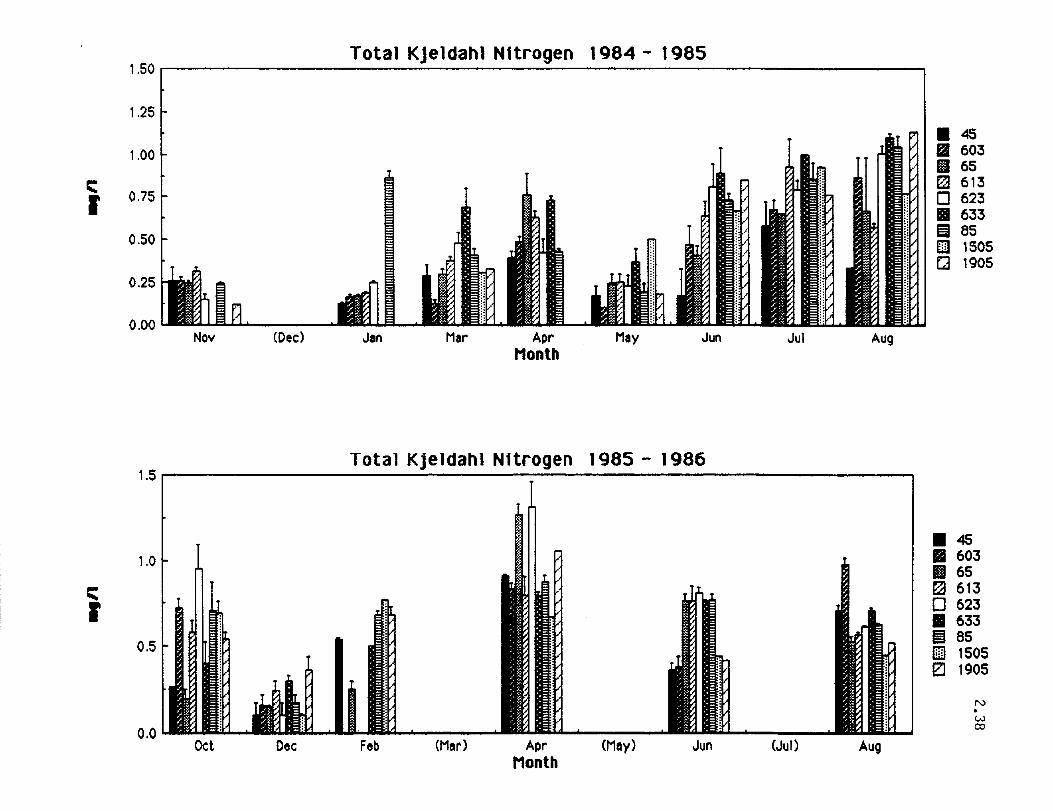
r::: r

r::: r

1.50

1.25

1.00

0.75

0.50

0.25

0.00 Nov (Dec)

Total KJeldahl N1trogen 1984 - 1985

Jan Mar Apr Month

May Jun Jul Aug

Total Kjeldahl N1trogen 1985 - 1986 1.5r. ---------------------------------------------------------------------------------------~

1.0

0.5

0.0 Oct Dec Feb (Mar) Apr

Month (May) Jun (Jul) Aug

.45 fa 603 a 65 ~ 613 o 623 • 633 Ii 85 [] 1505 Q 1905

.45 II 603 III 65 ~ 613 o 623 • 633 Ia 85 IiliI 1505 IZl 1905

N

W CXl

Figure 2.11. Total phosphate measurements made during the Lavaca Bay

study, 1984-1986. Units are mg P /Iiter. Error bars represent

range of duplicate samples taken about 20 minutes apart.

2.39

Total Phosphate 1984 - 1985 O.5~i---------------------------------------------------------------

Total Phosphate 1985 - 1986

2.41

Figure 2.12. Chlorophyll i1 measurements made during the Lavaca Bay. study,

1984-1986. Error bars represent range of duplicate samples

taken about 20 minutes apart.

c::: • •

c::: =:

Chlorophyll a 1984 - 1985 100 i I

80

:[ 20

o Nov (Dec) Jan

100

80.

.0 [

40

20~ .- II 0 1

Oct Dec Feb

J

Mar Apr

Month May

Chlorophyll a 1985 - 1986

'I 1IiiiI;:a:;; I I

(Mar) Apr (May) Month

.45 iii 603 m 65 ~ 613 o 623 .. 633

1 e 85 rn 1505 EJ 1905

Jun Ju\ Aug

. • 45 III 603 II 65 E21 613 o 623 • 633 ~ 85 Il] 1505 o 1905

.I- II I N . .j::>

-" ... ·;1;;11 Q ea':'" I N

Jun (Jul) Aug

Figure 2.13.

2.43

Pheopigment measurements made during the Lavaca Bay study,

1984-1986. Units are J-Ig chlorophyll equivalents/liter. Error

bars represent range of duplicate samples taken about 20

minutes apart.

, • •

, =:

Pheoplgment 1984 - 1985 20ri------------------------~~------------------------------------~

10 r 1 T

o Nov (Dec)

I_~ '-

Jan Mar

j

Apr Month

May

.45 II 603 III 65

rI I I I ~ 613 o 623 • 633 Ei 85 {!iJ 1505 El 1905

Jun Jul Aug

Pheoplgment 1985 - 1986 20,i------------------------~------------------------------------~

.45 1:1 603 011 65

10 r I ~ 613 o 623 • 633 ~ 85 [J 1505 Ed 1905

N . ..,. 0 1 Col .;I(t;;11 '1"":1;:;1. a !IEI;:VI I

..,. Oct Dec Feb (Mar) Apr (May) Jun (Jul) Aug

Month

2.45

Figure 2.14. Phytoplankton cell counts and biovolume estimates made during

the Lavaca Bay study, 1984-1985. Error bars represent range

of duplicate samples taken about 20 minutes apart.

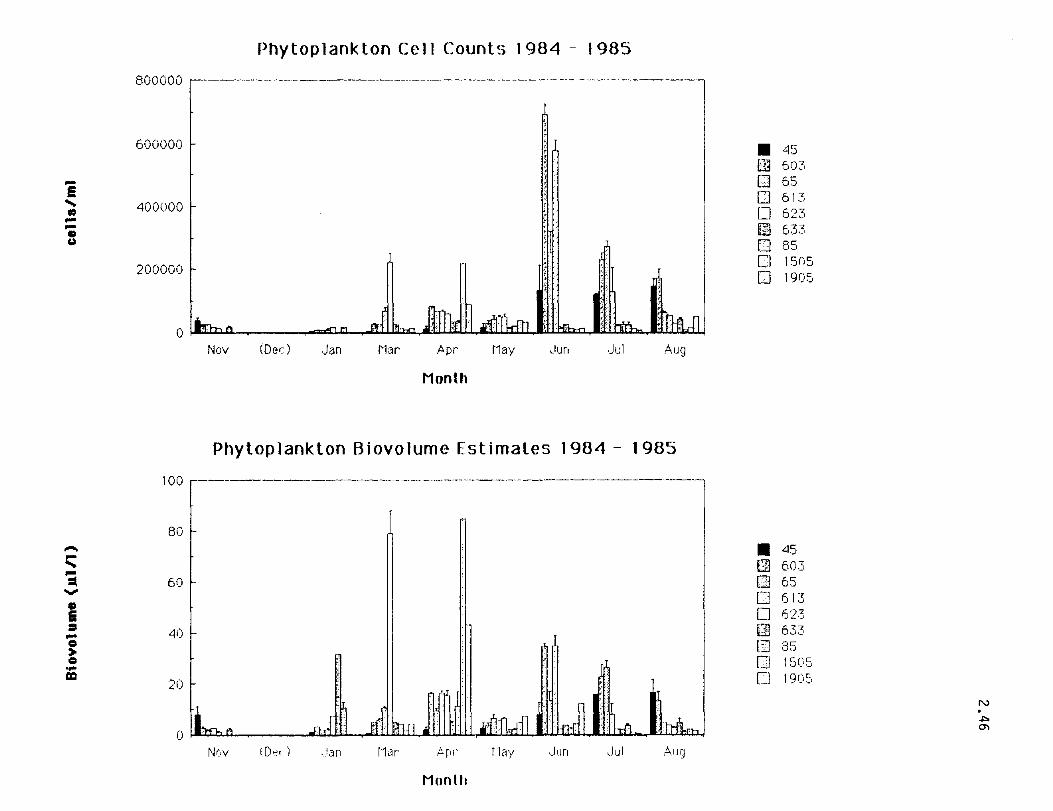
-e ..... ., --• ~

..... :::: -=. ...,. • e :J -o > o ...

eD

Phytop lank ton Ce J J Counts 1984 - 1985

800000 ,..----------------.-.-----.. - .. -------.- -- --.-------. ---------. -----.---------.-~

600000 r- Id I

400000 r iJ "

200000 l- II II mill nIT

o I bb, I) , -zy-=[] 1'1 Jii I ITt"" wlliioon ilIll \.dTJ I\HktMJ 1111-!r!b, It I M;W I I , Nov (Dec) .J,m Mar Apr t1ay ,IUrI .Jul Aug

Month

Phytoplankton Biovolume Estimates 1984 - 1985

100 --------------.---------- --.- --------.--------.- -------.-----.--------------

80

60

"1i)

20

o Ian be gOJ H __ I .jill -I tq t1! • [-I! I'Jl'l • I j-I fO -, I.'! I n,n!! Rep Un-t. •• :1' t FtDJ r , 1··Joy i.D~c ) ._.!an 1-1ar f. PI' flay .Jl.IrI ,.IIJ I -"·1.19

Mont II

• "15 Bd 6cX', Cl 65 [] 613 o 623 ~ 633 o 85 0 1505 o 1905

• "15 E] 603 o 65 [] 613 o 62-5 fJ3 6-' i-. , ')'_'

[J 85 [] 1505 [1 19V.',

N

-I'>

'"

Figure 2.15.

2.47

Phytoplankton cell counts and biovolume estimates made during

the Lavaca Bay study, 1985-1986. Error bars represent range

of duplicate samples taken about 20 minutes apart.

Phytoplankton cell counts 1985 - 1986 15000 r, ----------------------------------------------------------------~

"'" I • 45 4 = 10000 III 603 ..

>< til 65

i m 613 o 623 ... II 633 u .. Il!1[j 85

5000 ., o 1505 - o 1905 - fa 8

0 Oct Dec Feb (Mar) Apr (May) Jun (Jul) Aug

Month

Phytoplankton B1ovolume Est1mates 1985 - 1986

100

80 .... .45 =::: B!l 603 -• 60 m 65 ... E:J 613 I o 623 • 40 III 633 -• ~ 85 ~ !ill 1505 ' ..

11:1 20 [] 1905

0 N . Oct Dec Feb (Mar) Apr (May) Jun (Jul) Aug ..,.

co

Month

Figure 2.16

2.49

Relative abundance of phytoplankton taxa during the Lavaca

Bay study, 1985-86. All stations combined.

1,00

,90

,80

,70

,60

,50

.40 ,30

,20

,10

,00 Cyanophytes

.Oet85

LaDaco Day Phytoplankton 1905-06 Relatiue Abundance

Diatoms Chlorophytes Cryptophytes Oi nofl agell ates Fl agell ates & Monads

III Dee 85 II Feb 86 [ill Apr 86 o Jun 86 ~ Aug 86

N

(J'1

o

Figure 2.17.

2.51

Relative total biovolume of phytoplankton taxa during the

Lavaca Bay study, 1985-1986. All stations combined.

1.00

.90

.80

.70

.60

.50

.40

.30

.20

.10

.00 Cyanophytes

• Oct 85

LaUDea Bay Phytoplankton 1985-06 Relatiue Biouolume

Diatoms Chlorophytes Cryptophytes Dinoflagellates Flagellates & Monads

l1li Dec 85 fIi Feb 86 ill Apr 86 o Jun 86 !;; Aug 86

N

01 N

Figure 2.18.

2.53

Total phosphorus (mg P/I) vs light extinction during the Lavaca

Bay study. Yl 1984-85, Y2 = 1985-86. The extinction

coefficient, k (m- 1), was estimated from secchi depth assuming

that the depth of 1 % surface irradiance is 3x the secchi depth.

The equation is k = secchi depth/1.54.

included to show the trends in each year.

Regression lines are

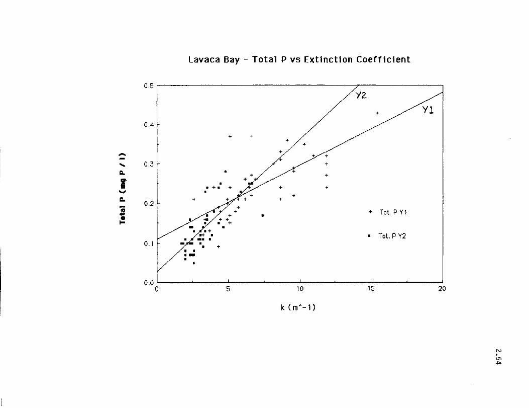
..... -.... c.

r ... c.

i • I-

Lavaca Bay - Total P vs Extinction Coefflc1ent

0.5 I 7

+ , / 0.4,

+ + +

~ ./

..,/ + A

+ + / ./ 03[ •

+ + • ++ff • +.

+ • + +

0.2 Tot.PY1 + /./+

+ • •

• Tot. P Y2 0.1 ~ ~ -;" " - - +

O.O~I ------~----~------~----~------~----~------~----~ o 5 10 15 20

k (mA-l)

N

U'1 ~

Figure 2.19.

2.55

Chlorophyll (JLgfl) + N03 (JLM/2) vs light extinction during the

Lavaca Bay study. Chlorophyll + N03 is a very rough estimate

of the potential for light-dependent primary productivity in

terms of nitrogen. In phytoplankton, JLg Chi a corresponds

roughly 0.5 JLmole cell nitrogen (C:Chl .:: 50; C:N :. 7). Yl =

1984-85, Y2 1985-86. The extinction coefficient, k, was

estimated as in Fig. 2.18. Regression lines are included to

show the (weak) trends in each year. One extreme value from

Sta. 623 in March 1985 has been excluded.

~

i III In • +

so

40 r

30 I-

A 20 u

10

o o

+

•

Lavaca Bay - Chl (J,lg/1l"N03 (J,lMl/2 vs I<

Chl+.S"N03 YI

+ Chl+N03/2 Y2

+

• • + ••• •

+

S

+

+

• +

+

+

k (mA-1)

+

+

10

+

+

l5

N

(J'J

C1'\

Figure 2.20.

2.57

Phosphorus and nitrogen in Lavaca Bay 1984-1986. Upper

graph: x - dissolved phosphate (mg P II), filled boxes - total

phosphate (mg P/I). Lower graph: x - nitrate (mg N!I); filled

boxes - total Kjeldahl nitrogen (mg Nil). Note that high

phosphorus values between 23-30 ppt are from station 1505 and

1905. Human perturbation of sediments III and near the

channel is a suspected influence.

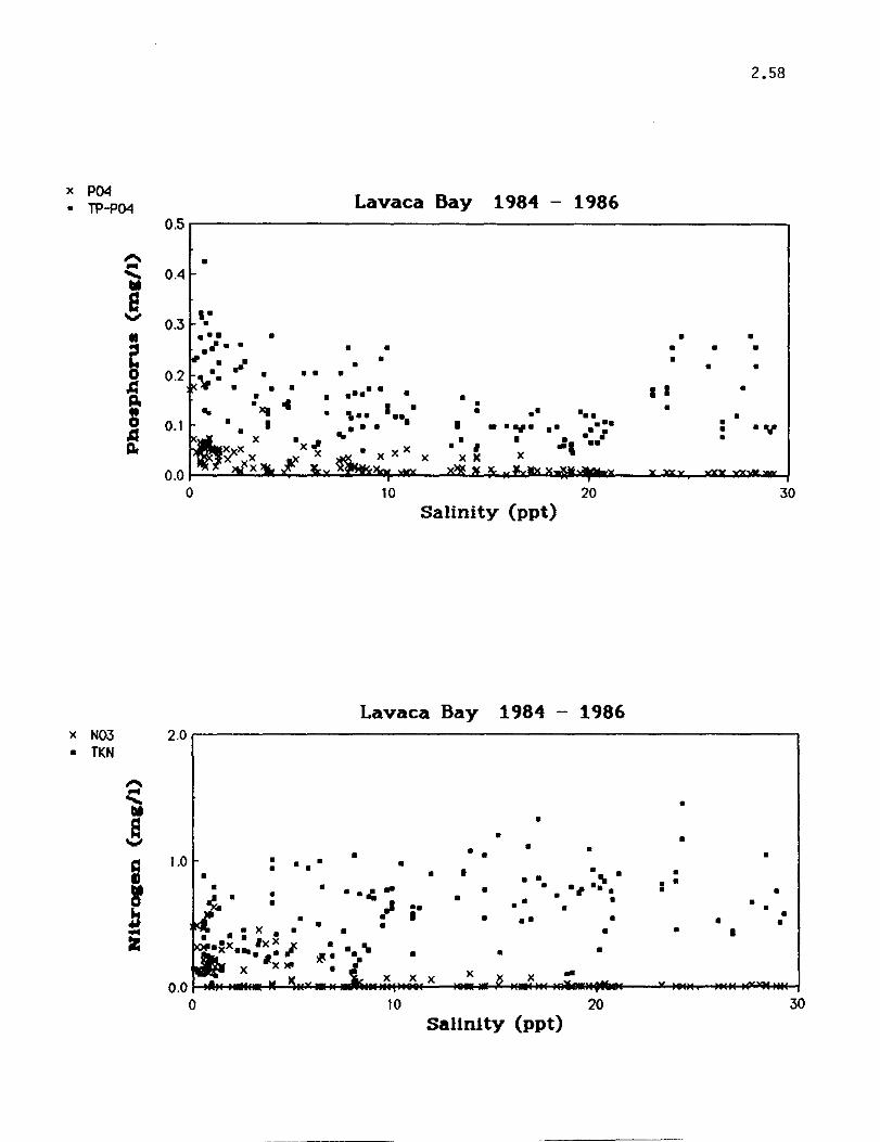
2.58

x P04 • TP-P04 Lavaca Bay 1984 - 1986

0.5

,.... • ... ...... III e

..." .. • • •

~ • • • • • • • •

• • • • • • •

J:I • • g, • • .. .. XiI 0 0.1 • I

.c:I • Dc

• ••••• • • • • , .. ••••

•• • '"

• • • •• • •• I . ..... •• ••• • • • • .:, • • • ••

I I • • • • • .y

•

0.0 0 10 20 30

Salinity (ppt)

Lavaca Bay 1984 - 1986 x N03 2.0 • TKN

,.... ... ...... III •

e • ..." • •

• • •

i • • • • • • • • • • • • • •

• • • .. • • • .11. .. • • . , ... • • • • • • • ,) • • • • a •• • • • • • • •• • • • • • • • • • • 2: • • •

x x x x .. 0.0

0 10 20 30 SaUnlty (ppt)

Figure 2.21.

2.59

Phosphorus (mg P II) and nitrogen (mg Nil) in Lavaca Bay 1984-

1986. Note that high phosphorus values between 23-30 ppt are

from station 1505 and 1905. Human perturbation of sediments

in and near the channel is a suspected influence.

... ~ a foe

"... ... ..... .. e '" Z ... ., ~ a foe

"...

I .. e ..... Cl. .. e '" Z .. ~ ... ..... Cl. .. ~ a foe

2.60 Lavaca Bay 1984 - 1986

y ·0.2138 - 0.004)( R = 0.43 0.5.-------------'-------------------, +

0.4 r ++ +

++ 0.3.tt+++

++ l + +1+ +

+ itt ++ 0.2 r +

+

+

+ ++ +

+

+

+ +

+ +

+

-It:l: 0.1 I-

++ + t j

+

++++ + + + + *++ :I: +

+ -It+ + + ++

+ +

+ + + + + +

+ + + :I: ** +

+ :I: + +V +

O.OL---------~--------~I--------~---------~I--------~------~ o 10 20 30

SaUnity (ppt)

y - 0.5614 + O.0079x R - 0.24 2.------------------'----------------------------------.

+ +

+ + + + + + + +

+. t ++* + + + + + + + .. + + + + + + + :I: + f it- + +4 + + + +~ ++ + + + + ++ + + +

Itt+* + +

++t t+ + + + + + + + + + + + + + ft.+ + ++ + + + + * t+ + + +++~ + + + +i++* ~+ + ++ it + ++ + I .i 0 0 10 20 30

Salinity (ppt)

Y = 0.496 - 0.0148x R = 0.47 2

+

+ + +

1 I- +:1: + + +

+++ ++ + + \+ +

+ t + ~t++++++ + + + ++ + +

+ + + + + + + + + t+ (f:l:+:+ * +

f+ + *-It + ",+ + +..,.++ ++ ~l+ +** *+-It +

+ + I i' + + + +~ -.L

0 0 10 20 30

Salinity (ppt)

Figure 2.22.

2.61

Light-limitation of primary productivity as a function of water

clarity and incident irradiance, scaled to that which saturates

photosynthesis. From Table 2.31 (Cullen, unpub1.). This figure

shows that when the depth of the mixed layer is greater than

the I % light level (k/z > 4.61), photosynthesis I2IT unit

chlorophyll in the mixed layer is light-limited.

light limitation of Net Photosynthesis in MiHed Lauers Curves for Different Uillues of lolls

Net Photosynthes1s

(theoret1cal max = 0.9)

1.00

.80

.60

.40

20

r. ~·'··"'.~.' .. ''''w.' .... '' .....•. '''.'.~ .... ' ..... '..,.'..., ...... ".·.·'w., .. ,." ...• ~ ..

. ~~~~~ ... w·' .. "' ......... ~' ............ ,._ .. w

I ! ! --, , . .00

-.20 .0 2.0 4.0 6.0 8.0 10.0 12.0 14.0 16.0 18.0 20.0

Scaled L1ght extinction: k/z

- 10/1s=1

- 10/15=1.5

10/1s=8

10/15=20

N

0'1 N

Figure 2.23.

2.63

Chlorophyll (filled diamonds) and pheopigment (open triangles)

at Station 85 at the surface on April 9, 1986. From Davis,

1986.

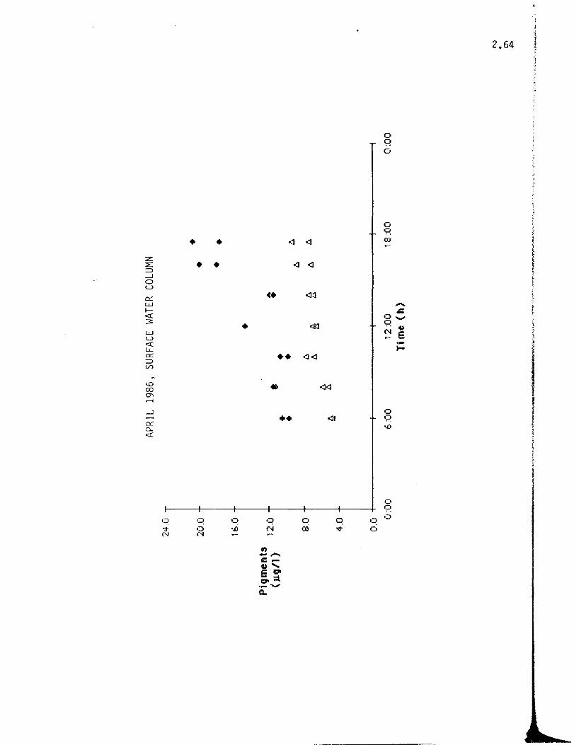
• • :z:: ::E • • =:J --' 0 L>

n:: w f-co:: 3:

w L> co:: l..L.. n:: =:J (/")

1.0 co 0'> ...... --' n:: 0-co::

•

.:1

.:1

c.

••

•

q N

••

.:1

<I

<1:3

0:1<1

o (0

.:10:1

<II

o q o

0 q ())

..... .&:

0..., q N

0 q '0

o q

() I:)

o

4> e .-l-

2.64

, ~

"

I I ! i I ,

Figure 2.24.

2.65

Chlorophyll (filled diamonds) and pheopigment (open triangles)

at Station 85 at the surface on June 6, 1986.

1986.

From Davis,

••

•• •

z: -!to ::E ::::l -' • 0 •• u

cr: • w l-e,; • • :3

w •• u e,; • u... cr: ::::l • • V> .. ill 00 c:ro 0-<

w :z: ::::l '""J

0;) C) oJ q "3" oJ ·0 N N ,'I

., -,-.. C ~ 41 " E '=" '=" ::I. .- --Q.

<1'-1

Co:]

<1<1

<I

<13

<1<1

<1<1

<II

.,:]

.j

<i:]

'-1

CI () (Q V

<I

0;)

0

o e> o

0 0 0)

...... .c

':::1 ....... e>

~ N E .-l-

0 q ' ...

0 I~

0

2.66

Figure 2.25.

April 1200 h, vater column

Photosynthetic performance of phytoplankton at station 85 in April 1986. From Davis (I986). Photosynthesis vs. irradiance was determined for samples from the surface (triangles) and bottom (I.4 m; filled diamonds). These data and other measurements showed that the water column was uniform with respect to phytoplankton biomass and physiological capacity and that rates of photosynthesis were inconsistent with severe nutrient-limitation of growth rate. Data such as these can be used to model light-limitation of primary production and to estimate daily primary production in a turbid estuary (Davis et at., in prep.).

2.67

Figure 2.26.

2.68

Pigments associated with the microphytobenthos at stations 613

and 623. Data collected by H.L. Macintyre.

determined fluorometrically after extraction in

Pigments

acetone.

Pigment data collected in this manner must be intrepeted

cautiously. These figures show that benthic pigment can vary

consistently between stations and that the amount of pigment

in the upper 5 mm of sediment is similar in magnitude to the

amount in the overlying water.

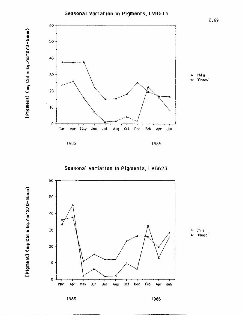
..... e e In

I Q ..... N • e ..... cr

"" II ... .c: U CJI e ....,

.... ., c:

~ CJI ....

Q. ....

..... e e In I

Q ..... N • e ..... cr

""

Seasonal Variation in Pigments, L VB613

60~-----------------------------------------,

50

40

~1 -0- ChI a ..... "Phaeo··

20

1 10

Mar Apr May Jun Jul Aug Ocl Dec Feb Apr Jun

1985 1986

Seasonal variation in Pigments, LVB623

60.----------------------------------------.

-0- ChI a ... ..... "Phaeo" .c: U

r 20

.... ., c: tI 10 e II1II -a. ....

Mar Apr May Jun Jul Aug Oct Dec Feb Apr Jun

1985 1986

2.69

Figure 2.27.

2.70

Photosynthetic performance of the microphytobenthos.

Photosynthesis vs irradiance for two adjacent samples of

sediment, 0-1 mm. Autotrophic potential is demonstrated.

Similar results have been obtained for sections of sediment

deeper than 5 mm. (MacIntyre, in prep).

12

10 -

8 - •

o -8

c o -

6

4

• 0 0

0 0 • •• ...

(.)

~ 2 0

-= E ~ a..

SJ85 0-lmm, 7/27/86

00 • • <I> 0 0 • •

• • •

0

O~--~----~,~--------~--~-----~,--~----~

o 400 800 1200 1600

P.F.D. (J1Ein/m~/s)

SJ85 0-) mm, 7/27/86

12 ...... .s::. .... ., 10 -.s::. U I:» 8 -::l .... U I:» 6

::l ..... c 4 0 -... (.) ~ 2 -= 0 ~ a..

0 , ,

0 400 800 1200 1600

P.F.D. (J1Ejn/m~/s)

2.71

o Serifs '" • Serits B

~rifS '" SeritsB

Table 2.1 2.72 LAVACA BAY 1984 - 1986

Comparison or Year 1 vs Year 2 Nonparametric Hann-Whitney U Test

(stations 1505 and 1905 excluded from this analysis)

1984 - 1985 1985 - 1986

Median Median 5i ificance

Air Temperature ("C) 24.0 27.6 ••

Waler Temperature (·C) 24.8 25.5 ns

Salinity (ppt) 2.50 9.13 """

5ecchi Depth (em 24.5 47.3 •••

pH 6.10 8.22 •

Dissolved Oxygen (mgt!) 9.00 6.60 ns

Ammonium (mg!l) .004 .007 .10>p>.05

Nitrile (mgtl .001 .000 .". Nitrale (mgtl .017 .001 "".

Phosphate (mg/l) .035 .006 •••

Tollli Kjeldahl Nitrogen (mgtl .400 .585 •

T olal Phosphale mg/l) .217 .115 •••

Chlorophyll II (~g/l) 9.64 6.34 ••

Pheopigmenl (~gtl 4.60 2.66 •••

The symbols indicale the probablility level. No correction for multiple testing has been applied.

• <.05 " " ( .0 1

...... <.001

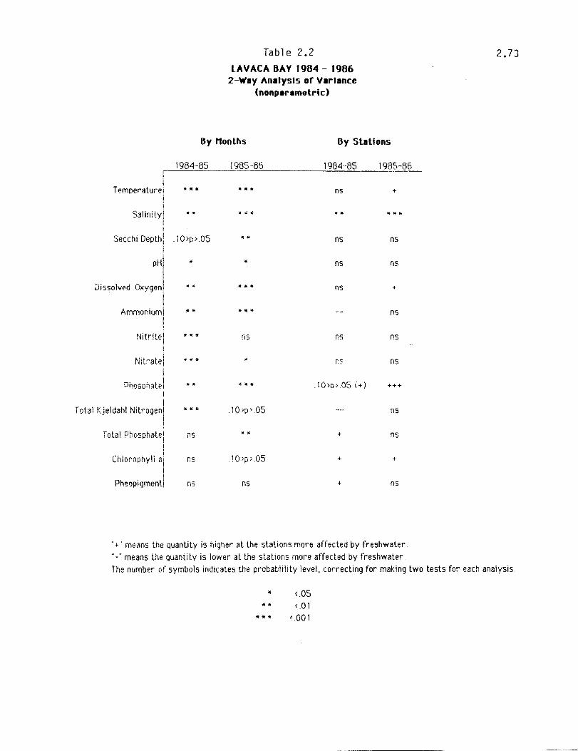
I Temperature;

i i

Salinity! I !

Sec chi Depth! i ,

PHI

Dissolved Oxygenl

I Ammoniumi

! Nitrile!

! !

Nitrate! !

Phosphatel I i

Total Kjeldahl Nitrogen! I ,

Tota! PhOSPhate: I !

Chlorophyli ai !

Pheopigmentl

Table 2.2

LAVACA BAY 1984 - 1986 2-WIY Anllysls or Vlrllnce

(nonplr.metric)

By Months By Stations

1984-85 198586 1984-85 1985-86 ----

"ill''' ••• ns +

.. "' ... " • • * JoO •

.10>p>.05 .. ns ns

• • ns n::.

" " *,.. ns +

. " ••• ns

"'"~!It ns ns ns

.. ioIf '" • ns ns

" . '" if 111- . 1 0 >o} .OS (+) +++

••• .10>p'.05 ns

ns !II! !IJ + ns

ns 10'p'.05 + +

os ns + ns

., T' means the Quantity is higher at the stations more affected by freshwater

"-" means the Quantity is lower at the stations more affected by freshwater

2.73

The number of symbols indicates the probablility level. correcting for making two tests for each analysis.

•• <.OS <.01

(.001

Table 2.3 lavaca Bay

CONDUCTIVITY AND SALINITY 1984 - 1985

Measurements on the day of Nulrient Sampling

2.74

Note: values from 1905 and 1505 in April are Questionable.

mmho/cm

November

45! 4.8

January March April May June July August

.6 2.5 6.1 .5 1.5 1.3 6.0

603 5.8 , 1.2 1.1 , 2.0 2.7 9.0

65 6.5 1.8 1.2 1 1 15 ~.8 4.4 17.0

613 13.1 7.5 5.5 1.8 4.B 3.7 13.0 23.0

623 14.9 20.0 8.4 2.8 2.8 10.0 14.0 23.0 633 12.5 2.2 16 13.5 110 220

85\ 12.5

1505

21.5 10.0 3.6 6.8 16.0 15.0 26.0

21.9 30.5

19051 10.9 31.7

Salinity algorithm: S (ppt)= a*(Cb.l where C is conductivity

(determined by log regression of ,:ondu,tivily

a b '15 salinity in laboratory calibration) Up to March 0.3708 .129

After March 0.4321 1. 1 19

Salinity ppt

November Januar'[ March AQril May June .July August Average s.d

45i 2.2 .2 1,0 3.3 .2 .7 .6 3.2 1.42 128 603! 2.7 0 .5 .5 ,3 9 1.3 S.i 140 169

65! 3.1 .7 .5 .5 ~ 2.5 2.3 10.3 2.55 3.29 . I

6131 6.8 3.6 2.5 .8 2.5 1.9 7.6 14.4 5.02 4.48

623i 7.9 10,9 4.1 1.4 1.4 5.7 8.3 14.4 675 4.57

6331 6.4 1.0 .7 8.0 6.3 13.7 6.03 4.82

85

1

6.4 11.8 5.0 1.8 3.7 9.6 8.9 16.6 7.98 4.78

1505 13.7 19.8

1905! 6.3 20.7

Average I 4.83 4.55 2.86 1.33 1.35 4.18 5.05 11.10 4.39 s.d., 2.46 5.45 2,37 .98 1.30 3.58 3.55 5.14 4.36

(note: stations 1505 and 1905 excluded from averages)

Temp:C November January

45 14.9 6.6

6031

14.7 5.5 65 15.5 5.2

6131 16.3 6.0 , 623 14.6 6.5 633

85 14.9 6.3

15051

19051 IS.1

, Average I 15.11 6.03

s.d. .61 .59

Dissolved Oxygen. mg/l

November Januar 45 9.2 13.5 ,

603! 9.1 14.4

6s1 9.4 13.6 ,

613\ 6.9 16.2 623 9.0 16.6 , 6331

65 9.2 15.6 1505

1905 10.2

Average I 9.29 15.02

5.d·1 .43 1.36

Table 2.4 lavaca 8ay

HYDROGRAPHIC PARAMETERS 1984 - 1985

March June Jul 15.2 26.5 32.3 31.3 16.1 24.8 27.0 7 ..... f\ 31.0 VL...V

16.1 22.5 26.0 27.3 31.6 30.3 17.6 24.3 26.3 27.5 30.5 30.5

165 17.5 27.0 30.0 26.6 30.0 17.0 21.0 25.6 28.0 28.3 26.5

16.3 20.3 25.0 26.0 28.8 29.6

16.5 20.8 31.0 16.4 22.7 30.5

16.42 22.06 26.17 27.75 30.42 30.16 .72 2,41 .69 1.13 1.51 .91

r1arch June Jul 9.2 7.5 11.0

9.8 10.4 7.2 8.5 11.0 9.0 9.4 10.8 8.6 8,4 10.6 7.4

10.6 10.4 10.4 9.1 5.5 9.2 13.0 6.4 7.8 6.1 7.5 8.2 10.6 8.0 7.2 7.7 7.3 7.6 9.1 9.2 6.0 7.2 6.5 7.7 6.2 6.4 6.3

8.5 6.5 6.1

9.62 9.19 8.00 8.06 6.31 8.33

1.45 1.06 1.22 .66 2.05 .73

* Sl 45 is 8/17

2.75

Average s.d.

22.22 9.00 ...... .II n ,.,,, LL.. .L.""'t ~ • .L,-"_'

21.62 6.99 22.39 8,46

21.35 8.79 24.75 4.73 2: .14 6.26

22.77 7.45 21.18 7.05

22.14 7.84

Average s.d.

9.35 2.09 9.93 2.15 9.78 1.91

;0.41 2.47 9.83 ~'.25 6.09 1.27 9.09 2.69 7.63 1.16

6.33 1.69

9.37 2.31

Table 2.5 2.76

lavaca 8ay HYDROGRAPHIC PARAMETERS 1984 - 1985

pH

November Januar March April .May June Julv . , August Average s.d.

45 8.3 8.3 8.0 8.0 7.6 7.9 8.1 8.00 .23 603 8.6 8.4 8.5 8.2 6.9 7.9 8.\ 8.06 .56

65 8.4 8.5 8.1 7.9 7.3 7.9 8.1 8.02 .37 613 6.3 6.4 8.2 6.5 6.4 7.9 B.1 8.24 .19 623 B.4 7.2 B.9 7.4 B.O 7.9 B.l 7.97 .56 633 8.8 B.O 7.7 B.O 8.1 806 .41

65 6.2 9.0 B.4 B.l 6.2 6.0 6.1 6.26 .35 1505 7.9 8.4 7.5 7.93 .45 1905 8.3 8.0 8.3 7.2 795 .52

Average I 8.34 8.27 6.29 8.07 7.72 7.91 7.35 B.09 8.07

s.d .1 .\4 .59 .34 .32 c· ,.J I .02 ,') ~ .02 AO

Seeehi Depth. em

November Januar' March June Jul Average s.d. 45 60 20 23 23 36 \7 34 29.0 \4.3

603 30 20 30 \8 \6 3\ 23 31 24.9 6.3 65 41 20 18 18 25 42 31 35 28.8 9.9

613 18 45 22 13 27 31 23 30 26.1 9.7 623 52 50 39 15 \6 13 ? --'I 28 29.6 15.6 633 30 14 10 13 ~c

L,\ 27 19.6 6.5 B5 45 90 36 13 27 16 47 47 40.1 24.2

Average I 41.0 40.B 2B.3 16.3 20.0 26.0 27.1 33.1 28.6

S.d. 15.2 27.6 7.7 3.6 6.5 11.9 9.7 6.8 14.4

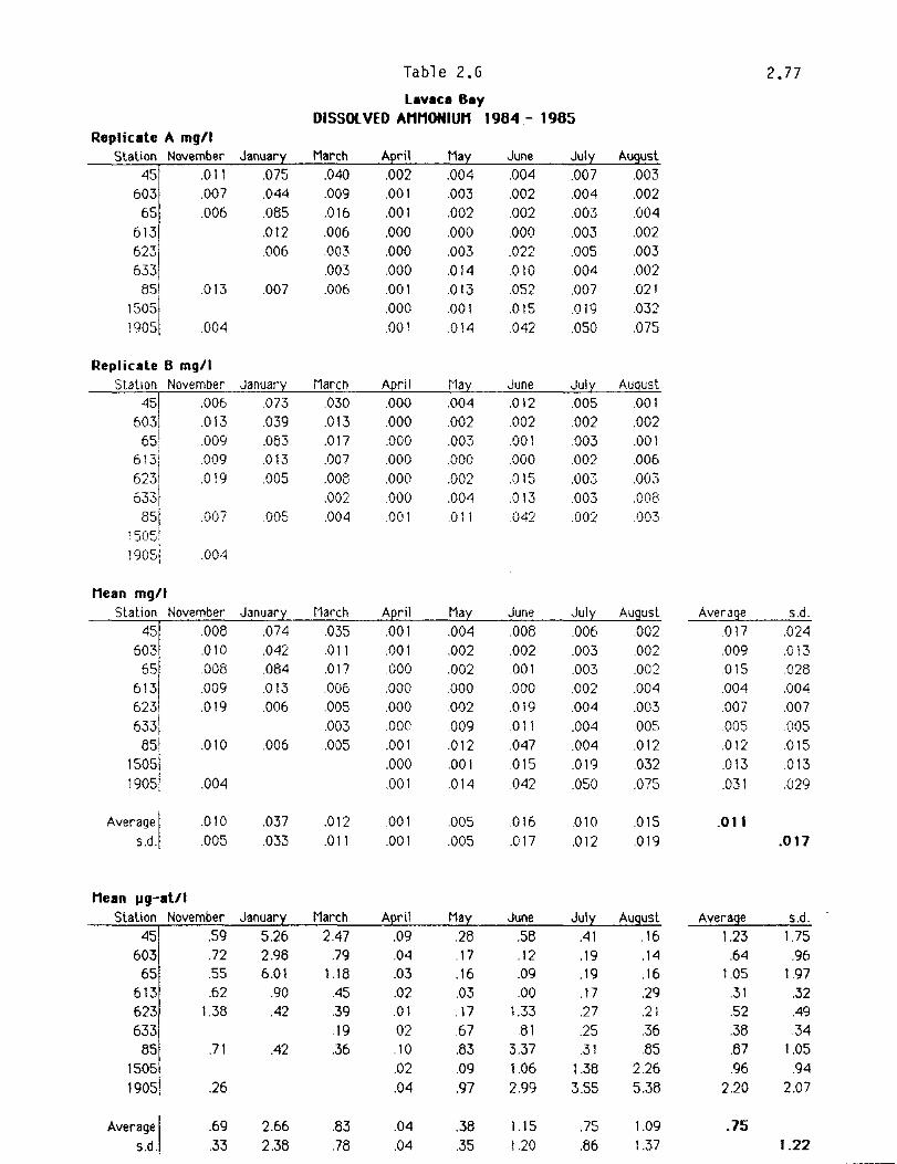
Replicate A mgll Station November

45 .011 603 .007

651 .006 6131 623

1

6331 851 .013

1505\ 1905 .004

Replicate B mgll StatIOn November

45 .006 603 .013

65 ,

~~~I 6331

8S1 ~505l

.009

.009

.019

.1')07

1905i .004

Mean mgll Station November

45 .008

603 65i ,

6131

623

633

55 1505

1905

Average I s.d·1

Mean pg-at/l

.010

.008

.009

.019

.010

.004

.010

.005

Januar

.075

.044

.085

.012

.006

.007

Januar

.073

.039

.063

.013

.005

.005

Januar

.074

.042

.054

.013

.006

.006

.037

.033

Station November Januar

45 .59 5.26

603 65

613 623 633

55 1505

1905

Average I s.d ..

.72

.55

.62

1.38

.71

.26

.69

.33

2.98 6.01

.90

.42

.42

2.66 2.38

Table 2.6

lavaca Bay DISSOL YED AMMONIUM 1984 - 1985

March

.040

.009

.016

.006

.003

003

.006

March

.030

.013

.017

.007

.008

.002

.004

March

035

011 .017

006 .005

.003

.005

.012

.011

March

247 .79

1.18 .45 .39

.19

.36

.83

.78

.001

.001

.000

.000

.000

.001

.000

.001

.000

.000

.000

.000

001

April

.001

.001 000

.000

.000

.000

.001

.000

.001

.001

.001

.04

.03

.02

.01

02 .10

.02

.04

.04

.04

.003

002 .000

.003

.014

.013

.001

.014

.003

.000

.002

.004

.011

Ma .004 .002 .002

.000

.002

.009

.012

.001

.014

.005

.005

.17

.16

.03

.17

.67

.83

.09

.97

.38

.35

June

.004

.002

.002

.000

.022

.010

.052

.015

.042

June

.012

.002

.001

.000

.015

.013

.042

June

.008

.002

.001

000 .019

.01 !

.047

.015

.042

.016

.017

June

.58

.12

.09

.00 1.33

.81 3.37

1.06 2.99

1.15 1.20

Jul

.007

.004

.003

.003

.005 004 .007 .019

.050

Jul

.005

.002

.003

.002

.003

.003

.002

Jul

.006

.003

.003

.002

.004

.004

.004

.019

.050

.010

.012

Jul

.41

.19

.19

.17

.27

.25

.31

1.38 3.55

.75

.86

.002

.004

.002

.003

.002

.021

.032

.075

.001

.002

.001

.006

.003

.OOB

.003

.002

.002

.004

.003

.005

.012

.032

.075

.015

.019

.14

.16

.29

.21

.36

.85

2.26 5.38

1.09 1.37

Average

.017

.009

.015

.004

.007

005 .012

.013

.031

.011

Average

1.23 .64

1.05 .31

.52

.38

.87

.96

2.20

.75

2.77

s.d. .024 .013 .028

.004

.007

005 .015

.013

029

.017

S.d.

1.75

.96 1.97 .32 .49

.34 1.05 .94

2.07

1.22

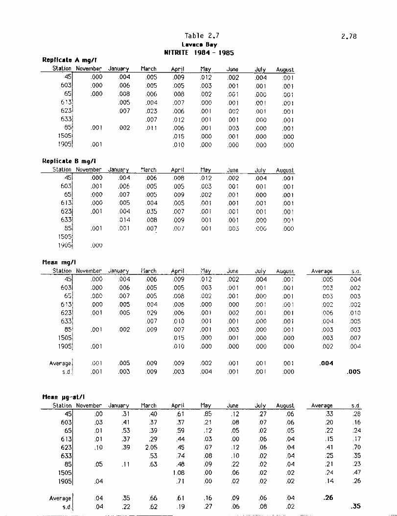
Replicate A mgll Slation November Januar

45 .000 .004 603

65

613

623. 633

85 1505

1905,

.000

.000

.001

.001

Replicate B mgll Station November

451 .000 603

1

.001 65 .000

6131 .000

6231 .001 633

851 .001

150~1 1 yt)~1 .001)

Mean mgll

.006

.008

.005

.007

.002

January .004

.006

.007

.005

.004

.014

.001

March .005 .005 .006

.004

.023

.007

.011

March .006 .005 .005 .004

.035

.008

.007

Station November Januar i1arch 45 .000 .004 .006

603 .000 .006 .005 65

613 623 633

851 1505

1 1905

Average I sdj

Mean Jlg-atll

.000

.000

.001

.001

.001

.001

.001

.007

.005

.005

.002

.005

.003

Station November .Januar 45 .00 .31

603 65

613 623

633 85

1505

1905

Average I S.d.

.03

.01

.01

.10

.05

.04

.04

.04

.41

.53

.37

.39

.11

.35

.22

.005

.004

.029

.007

.009

.009

.009

March ,40

.37

.39

.29 2.05

.53

.63

.66

.62

Table 2.7 Lavaca Bay

NITRITE 1984 - 1985

.005

.008

.007

.006

.012

.006

.015

.010

April .008

.005

.009

.005

.007

.009

.007

.008

.006

.006 010 .007 .015

.010

.009

.003

.37

.59

.44 ,45

.74 ,48

1.08

.71

.61

.19

.002

.000

.001

.001

.001

.000

.000

May .012 .003 .002 .001 .001

.001

.001

.003

.002

.000

.001

.001

.001

.000

000

.002

.004

.21

.12

.03

.07

.08

.09

.00

.00

.16

.27

June .002 .001 .001

.001 002 001 .003 .001

000

June .002 001 .001 .001 .001

.001

.003

June .002 .001 .001

.000

.002

.001

.OO~,

.001

.000

.001

.001

June .12 .08 .05 .00 .12 .10

.22

.06

.02

.09

.06

Jul .004

.001

.000

.001

.001

000 .000 .000 .000

July .004

.001

.000

.001

.001

.000

.000

Jui

.004

.001

.000

.001

.001

000 .000 .000

.000

.001

.001

Jul .27 .07 .02 .06 .06 .02 .02 .02

.02

.06

.08

.001

.00i

.001

.001

.001

.001

.000

000

August .001 .001 .001 .001 .001 .001 000

.001

.001

.001

.001

.001

.001

.001

.000

.000

.001

.000

.06

.05

.04

.04

.04

.04

.02

.02

.04

.02

Average .005 .003 .003 .002 006 .004 .003 .003 .002

.004

Average .33 .20 .22 .15 ,41

.25

.21

.24

.14

.26

2.78

5.0.

.004

002 003 .002 010 005 .003 .007

.004

.005

S.d.

.28

.16

.24

.17

.70

.35

.23 ,47

.26

.35

Table 2.8 lavaca Bay

NITRATE 1984 - 1965 Replicate A mgt I

Stalion November Januar 45004 .487

603

65

613

623

633

65

1505

1905

.003

.002

.001

.000

Replicate 8 mgtl

.480

.584

.341

.063

.059

March .633

.490

.470

.141

.364

.235

.326

.219

.316

.118

.296

.220

.324

.099

.218

_--,So:.:l=:a t:.:.;i o:.:.;n'r-'-'N=-ov:..::e"-m:.::.be:.;.r---,J,",a,,,nu:..::a.:...ry,--~M:.:::ar:..;c=.h __ A£!:.i.L 451 .001 .493 .604 .462

6031 .001 .490 .514 .192

651 .002 .577 .496 .331

b

6-21J3

7·1 .002 .359 .129 .171

.000 .033 .501 .316

633. .245 .238

851 .001 .053 .268 .369

15051 1905i .001

Mean mgll Station November Januar

45 .003 .490

603 I

6"' ..II

6131 6231

6331

851 I

15051 1905 1

Average I s.d.,

.002

.002

.002

.000

.001

.000

.001

.001

Mcan Jlg-atll Stalion November

45 .19

603 .13

65 .14

613 .14

623 .02

633

.485

.581

.350

.048

.056

.335

.220

Januar 34.97

34.61

41.47

24.96 3.45

March . 618

.502

.483

.135 '133

.240

.298

.387

.165

March 44.17

35.86

34.47

9.65

30.91

17.14

.205

.323

.145

.306

229

.346

.099

.218

.259

.107

14.67

23.10

10.35

21.89

16.35

85

1505

1905

.08 4.00 21.27 24.73

Average I s.d.

7.11

.04 15.59

.11 23.91 27.64 18.52

.06 15.74 11.79 7.61

.139

.128

.012

.159

.568

.213

.006

.006

May .292

.145

.139

.010

.212

.441

.265

.142

.133

.011

.185

.505

.239

.006

.006

.170

.160

10.12

9.53

.80

13.23

3605

17.08

.41

.46

1215

11.41

June .002

.001

.002

.000

.015

.010

.064

.005

.005

June .038

.001

.006

.001

.014

.015

029

June .020 .001

.004

.000

.015

.013

.046

.005

.005

.012

.017

June 1.43

.06

.28

.00 1.05

.90

3.30

.35

.35

.86

1.24

Jul .172

.001

.001

.000

.001

.000

.001

.002

.002

July .164

.001

.00i

.000

.000

.001

.000

.001

.OO!

.000

.001

.001

.000

.002

.002

.019

.057

July 12.02

.06

.06

.00

.04

.06

.03

.11

.11

1.39

4.09

.001

.002

.003

.000

.000

.000

.002

.000

August .001

.000

.002

.001

.000

.000

000

.000

.002

.002

000

000

.000

.002

.000

.001

.001

August .10

.02

.16

.14

.00

.00

.00

.13

.02

.06

.07

Average .258 .167

.191

.061 123

.164

.123

.023

.039

.148

Average 18.43

11.94

13.65

5.75

8.62

11.75

2.79

s.d .

.237

.208

.231

.124

.166

.194

.142

.043

.082

_166

s.d.

16.96

14.89

16.50

8.1:14

11.88

13.85

6.61 10.16

1.62 3.07

2.76 583

10_54 13.43

Table 2.9 2.80

lavaca Bay DISSOI. YED PHOSPHA TE 1984 - 1985

Replicate A mgll Station November Januar:t March A~ri1 Ma:t June Ju1:t Augusl

451

.045 .177 .035 .071 .070 .038 .054 .015 603 .022 .170 .027 .045 .045 .066 .017 .023

65 .034 .182 .024 .043 .023 .052 .0iO .043

613 .131 .008 .017 .005 .031 .015 .038 623 .052 .003 .052 .028 .05b .017 .0.35 633 .007 .050 .053 .035 .015 .035

85 .044 .034 .023 .052 .018 .035 .010 .040 1505 .013 .000 .016 .010 .030

1905 .003 .008 .016 .002 .025

Replicate B mgll Slation November Januar:r March A~ri1 Ma:r June Ju1:r Auaust

45 .025 .200 .034 .073 .080 .040 .052 .015

603 .026 .183 .024 .036 .043 .068 .015 .020

65 .027 .193 .023 .034 .025 .026 .010 .043 613 .046 .150 .010 .024 .005 .028 .012 .043

623 .037 .040 .003 .041 .020 .061 .017 .013

633 .010 .045 .048 .038 .020 .043

85 .042 .018 .022 .052 .020 .0<12 o I'-} . I.:.. 103

1505,

19051

Mean mgll Slation November .Januar March June '\Ve~age S.d.

45 .035 .189 .034 .039 .053 .015 .064 .053 603 .024 .177 .026 .041 .044 .067 .016 .021 .052 .051

65 .031 .187 .023 .038 .024 .039 .0iO .043 .049 .055 , 613

1 .046 .141 .009 .021 .005 .029 .014 .040 .035 .044

6231 .037 .046 .003 .046 .024 .059 .017 .024 .032 .019

6331 .008 .048 .050 .036 .017 .039 .033 .016

55 .043 .026 02~, .052 .Oi9 .040 .011 .071 .036 .023

1505 .013 000 .016 .010 .030 .014 .011

1905, .003 .008 .016 .002 .025 .011 .010

Average I .036 128 .018 .037 .025 .038 .017 .034 .041 s.d.1 .009 .070 .011 .019 .024 .016 .014 .021 .041

Mean pg-atll Station November Januar March June Jul Average s.d.

45 1.13 6.09 1.11 1.25 1.71 2.07 170

603 .78 5.70 .83 1.31 1.42 2.16 .52 1.67 1.65

65 .98 6.03 .75 1.24 .77 1.25 .32 1.37 1.59 1.78

613 1.49 4.53 .29 .67 .16 .95 .44 1.29 1.23 1.42

623 1.18 1.49 .09 1.50 .77 1.90 .56 .77 1.03 .62

633 .26 1.54 1.62 1.18 .56 1.25 1.07 .53

85 1.39 .84 .73 1.69 .61 1.29 .36 2.30 1.15 .73

1505 .41 .00 .53 .32 .97 .44 .35

1905 .11 .24 .53 .08 .81 .35 .31

Average I 1.16 4.11 .58 1.20 .89 1.23 .54 1.10 1.33 S.d. .30 2.27 .36 .62 .77 .52 .46 .68 1.32

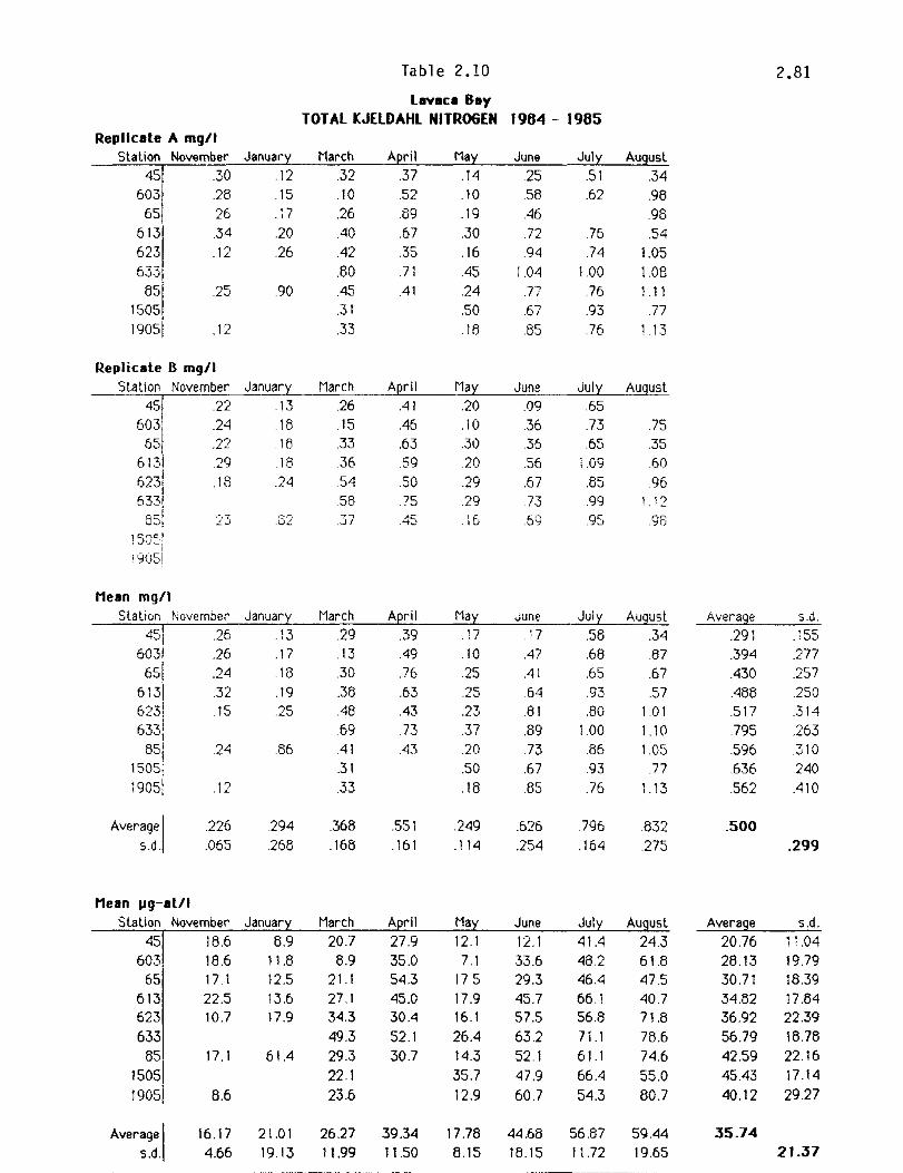
Replicate A mgll Station November

45! .30 603,' .28

65 .26

613 .34 623 .12 63.3,

851 1505

.25

19051 .12

Replicate 8 mgll

January

.12

.15

.17

.20

.26

.90

Table 2.10

Levaca Bay TOTAL KJElDAHl NITROGEN 1964 - 1965

March .32 .10 .26 .40 .42 .80 .45 .31 .33

April .37 .52 .89 .67 .35 .71 ,41

May

.14

.10

.19

.30

.16

.45

.24

.50

.18

June .25 .58 .46 .72 .94

1.04 .77 .67 .85

July .51 .62

.76

.74 1.00 .76 .93 .76

August .34 .98 .98 .54

1.05 1.08 1.11

.77

1.13

Station November January March April May June July August 45/-'-'=.2"'"2--"'='::':::. '-'13--'--'=':.-"'26'-'---'-=. 4-"1--'-'2"-'0'---"'.:::':0"-9---="".6"'-5--'-'=='-=-

6~~1 .24 .18 .15 .46 .10 .36 .73 .75 651 .22 .18 .33 .63 .30 .36 .65 .35

6131 .29 18 .36 .59 .20 .56 1.09 .60 62311 .16 .24 .54 .50 .29 .67 .85 .96 633, 58 .75 .29 73 .99 1.12

851 23 .32 .37 .45 16 69 .95 .96 1 5()S~

; 9~'5i Mean mgll

S la li on Novembe r Januar~y_-'.M""a;.:..rc""h,-----,A-"p,,-r;.;..i 1_'--M""a:..t..y_---=J:.::u"'oe'---_.::..Ju::.;.1 LY _.:..:A..:.;Ug;c:U=5 t 451 .26 .13 .29 .39 .17 .17 .58 .34

6031 .26 .17 .13 .49 .10 .47 .68 .87 651 .24 .18 .30 .76 .25 .41 .65 .67

5131 .32 .19 .38 .63 .25 .64 .93 .57 623i .15 .25 .48 .43 .23 .81 .80 101 633 .69 .73 .37 .89 1.00 1.10

85 1505 19051

Average I s.rj.

.24

.12

.226

.065

Mean J.lg-atll Station November

45 113.6 603 18.6

65 17.1 613 22.5 623 10.7 633

85 1505 1905

Average I s.d.

17.1

8.6

16.17

4.66

.56

.294

.2613

Januar 8.9

11.8 12.5 13.6 17.9

61.4

21.01

19.13

,41 .43 .20 .73 .31 .50 .67 .33 .18

.368

.1613

March 20.7

8.9 211 27.1 34.3 49.3 29.3 22.1

23.6

26.27 11.99

.551

.161

35.0 54.3 45.0 30.4 52.1 30.7

39.34 11.50

.249

.114

7.1 17.5 17.9 16.1

26.4 14.3 35.7 12.9

17.78

8.15

.85

.626

.254

June 12.1 33.6 29.3

45.7 57.5

63.2 52.1 47.9 60.7

44.68 113.15

.86 93 .76

.796

.164

Jul 41.4 48.2 46.4 66.1 56.8 71.1

61.1 66.4 54.3

56.87 11.72

1.05 .77

1.13

.832

.275

61.8 47.5 40.7 71.8 78.6 74.6 55.0

80.7

59.44

19.65

Average .291 .394 .430 .488 .517 .795 .596 .636

.562

.500

Average 20.76 28.13 30.71 34.132 36.92 56.79

42.59

45.43 40.12

35.74

2.81

S.d.

.155

.277

.257

.250

.314

.263

.310 240 ,410

.299

S.d.

1'.04 19.79 18.39

17.64 22.39 18.78 22.16 17.14

29.27

2J.J7

Tabl e ? .11 2 .82

lavaca Bay TOT AL PHOSPHA TE 1984 - 1985

Replicate A mg/l Slation November Januar March June Jul

45 .22 .36 .17 .37

603 .25 .35 .32 .28 .19 .28

65 .30 .24 .27 .14 .22 .16

613 .21 .27 32 .22 .14 .22 .17

623 .28 .33 .31 .26 .24 .18

633 .07 .33 .48 .29 .22 .19

65 .11 .05 .31 .22 .21 .13 .13

1505 .11 .07 .13 .09 .09

1905 .05 08 .16 .08 .06

Replicate B mg/l

Station November Januar March June Jul 45 .20 .37 .22 .35

603 .24 .39 .20 .26 65 .36 .25 .26 .11 .20 .21

613, ,), .25 .33 .21 .17 .22 .18 .L'

6231 .19 .37 .26 2~' .25 .18 633/ .23 31 .39 .26 .20 .19

851 .20 12 y. .21 .22 .11 .11 . v

lc:;nc:.l '~"-I 19051

Mean mg/l Slalion November Januar March Aprii Mav June Julv Au usl Averaae s.d.

45 .21 .37 .25 .30 .19 .36 .16 .263 .079

603' .24 .37 .31 .28 .20 .27 .20 .266 .059

65! .33 .24 .26 .13 .21 .18 .226 .070

613

1

.21 .26 .32 .22 .16 .22 . 17 ..... ....., ...... .054 .L":":

623 .24 .35 .29 .24 .24 .18 .256 .060

633 .15 .32 .43 .27 .21 .19 .264 .106 85 .16 .09 .30 .21 .22 .12 .12 .174 .076

1505 .11 .07 .13 .09 .09 .098 .024

1905 .05 .08 .16 .08 .06 .086 .042

Average I .205 .217 .300 .237 .188 .200 .152 .224 s.d·1 .042 .122 .039 .100 .051 .082 .043 .086

Mean Jlg-atll Slation November Januar March June Jut Average S.d.

45 6.8 11.8 6.2 11.6 8.47 2.55 603 7.8 11.9 9.9 9.0 6.3 8.6 6.6 8.59 1.91

65 10.7 7.9 8.5 4.1 6.7 5.9 7.28 2.25

613 6.6 6.4 10.4 7.0 5.0 7.0 5.6 7.17 1.73 623 7.6 11.2 9.2 7.9 7.9 5.7 8.25 1.93

633 4.8 10.5 14.0 8.7 6.8 6.3 8.50 3.43

85 5.1 2.8 9.7 6.9 7.1 3.9 3.9 5.60 2.44

1505 3.5 2.2 4.3 2.9 2.9 3.15 .79

1905 1.6 2.6 5.1 2.6 2.0 2.76 1.35

1 6.60 7.01 9.66 7.65 6.06 6.44 4.90 7.21 Average I

S.d. 1.36 3.93 1.27 3.21 1.64 2.65 1.36 2.79 -------------- --------

Replicate A P911

Station November Januar 45 21.0 3.1

603 9.7 .9 65

1

12.4 9.2 613 9.9 8.6

623/ 11.2 633

85 7.7 8.6

1505 1905 3.8

Replicate 8 pgll

Station November Januar:i 45! 20.6 3.6

6031 14.2 .9 651 13.1 9.1

613! 9.1 6.1 , 623 1

18A

6331 85i 6.4 15.5

Meltn 11911

Station November Januar 45 20.8 3.3

603 11.9 .9

651 12.8 9.2 613 9.5 8.3 623 14.8

6331

851 7.0 12.1

IS051 1905

Average I 12,41 8.11 s.d., S,43 S,42

Table 2.12

lavaca Bay CHLOROPHYLL. 1984 - 1985

(Corrected algorithm)

March June Jul 1.9 16.2 23.8

15.2 16.1 34.7 20.4 18.1 19.4 13.8 32.4 44.2 38.2 17.9 14.5 10.0

101.3 16.0 ! 1.4 3.5 1.2 36.5 13.6 9.5 9.9 4.1

6.5 20.4 16.0 7.7 3.5 4.6 13.5 7.6 3.9 3.9 15.8 6.6 3.8 3.4

March A~ril Ma:i June Jul:i August 2.1 10.6 16.6 23.1 17.4

14.6 1.2 15.6 41.9 18.3 18.2 23.: 15.9 15.7 31.1

46.7 34.3 18.4 17.6 8.8 94.5 8.4 10.2 4.1 1.1 35.3 15.2 7.9 9.8 4.6

7.3 23.8 17.8 8.0 4.5 3.4

March April Ma .June Julv AUGust 2.0 9.B 16.4 23.4 18.1

14.9 20.0 15.8 38.3 19.4

18.1 21.2 14.8 15.7 317 4S.4 36.2 18.2 16.0 9,4

97.9 12.2 10.8 3.8 1.1

3S.9 14.S 5.7 9.B 4.4 6.9 221 16.9 7.8 4.0 4.0

13.8 7.6 3.9 3.9 15.8 6.6 3.8 3.4

31.59 18.41 11.88 13.20 10.61 3178 9.32 4.23 12.10 10.32

2.83

Aver'age S.C. 13.42 8.15 17.32 1171

17.66 7.32 20.4S 14.12 23.44 3S.23

14.66 11.72 10.11 6.44

7.29 4.68 7,42 5.25

15.51 15.39

Replicate A Jlgll

Station November January 45 5.7 5.7

603 7.5 S.B 65 6.6 7.4

613, 8.4 2.7 623

1

"7 ... .J ... .1

633

85\ 6.0 2" .-'

1505 19051 1.3

Replicate 8 JlglI

Station November Januarl' 4,,1 5.7 5.0 .... '1

603; 9.8 5.2 651 7.3 9.0

6131 8.5 2.7 623\ 2.6 633!

851 5.7 2.9

Mean IIg/l

Station November Januar 45, 5.7 5.3

603\ 8.6 5.5 65

1

7.0 8.2

613 8.5 2.7 623 2.9 633

85 5.8 2.7 1505 1905

Average I 712 4.57 s.d. 2.22 2.14

Table 2.13

lavaca 8ay PHEOPI6MENTS 1964 - 1965

(Corrected algorithm)

March ~i1 Mal' June Jull' August 2.7 5.9 7.6 11.3 5.7

10.2 10.5 3.6 11.4 6.0 B.6 10.2 5.6 5.6 14.6

12.5 13.0 4.0 5.6 3.8 117 1.6 I1.B 3.9 1.6 8.7 6.9 12.1 3.3 2.6 3.1 7.8 7. i 10.6 1.9 2.3

3.6 3.3 .9 .9

4.7 2.7 .7 1.0

March ADril Mal' June Jull' AUQust 2.9 5.~, 6.7 12.7 A ..,

.,. I

10.5 7' '. , 4.3 10.3 6.4 7.5 10.9 5.1 7.4 13.7

9.7 12.~' 3.6 5.7 3.8 13 I 1.0 lOA 3.3 1.6 5.0 7.B 10.3 3.6 3. J

2.7 8.5 6.6 11.3 2.0 2.1

March Aprii Ma Jul August 2.8 5.fl 7 1 12.0 5.2

10.3 8.8 39 109 6.2 8.0 10.5 5.4 6.5 14.1

11.3 12.6 3,8 5.6 3.8 12.4 1.3 11.1 3.6 1.6 5.4 7.4 11.2 3.4 2.8 2.9 8.1 6.8 10.9 2.0 22

3.6 3.3 9 9 4.7 2.7 .7 1.0

802 6.96 6.61 5.07 4.21 3.76 3.55 3.46 3.94 4.10

2.84

Averaqe ' " :l.U.

6.25 2.77 7.76 2.63 8.5<1 2.90 6.90 3.83 5.49 4.73 6.65 3.34 5.19 3.17 2.19 1.49 2.27 1.54

6.28 3.56

Table 2.14 Lavaca Bay

PHYTOPLANKTON CELL COUNTS 1964 - 1965

Replicate A cells/ml

Sl~tlon November Januar' ~Iar(h April Mav ,June

45 ~,2524 4305 3968 3968 383 214717 124883 603 14823 9:145 28945 28945 ~~,7270 726216 212029 ,

651

22876 9181 2::.936 25936 54777 16:2351 :255731 613

1 1552_:· 9026 52832 52832 5275~ 610'216 206972

623! 14006 , 14.39:'. 254435 2~,443::;, ~Je20 1 11230 24536 6.33j 24See 2·4586 5356 1:,6'~6

E;5i 1 ':13:12 15717 201 j .. 1 ;j67(1 1 :=/)9~, , 1505j 6501 850! 38360 6384 1~320

19051 13020 13020 34314 1063<1 92;43

Replicate B cells/ml

~,tatlOn November ,Ianuar Maret, ,June .Julv

4S <159135 469", 3354 13429 31201 54116 113270 6031 23362 23913 83c;7E; 22201 65:',.:465 :'517 12 ,

65i 24~~ 7 i 6640 2·~::,88 64893 ~.0454 319250 289700 . "7j 61'-.li 14589 II :!30 7869:3 66604 46296 5~1EJ21 e 50731 F('" L-_It 9921 194678 56541 40616 17075 20619 -'" .... -1 O.:IJ! 103052 24691 ~1470~1 W324 24834 32783

i3Sl ::059:, :377"L 13889 3~291 21203 ;223~ .3 i 74e· 1505i 1 a ~c: 1 , .. ( .. Jj

Mean cells/ml

Statiofl Novernb"r· Jarluar·y r1arch April May ,June Julv 4c l

39255 450(! 3661 6199 15792 13~Ll17 121~)76 ")1 , 6031 19102 95.:15 26429 :,641 1 29736 689841 231871

I

651 23673 7911 25262 45414 42616 2SI0!::,0 272716 6<71 15056 10128 65865 59718 49525 578217 128852

I.J

\ "''''1-' 1196~. 142",95 224556 I 554Em 49409 14153 22578 f)L.:I! 1'7-1 U ... I,) 18052 24639 29645 11840 24834 24216

851 16973 14745 13889 32291 20658 10551 23420 15051 3501 8501 38360 838..:l 12320 19051 13020 13020 34314 10634 9843

Average I 21004 11325 45091 45188 32472 191342 94155 s.d. 1008 I 10081 73604 61317 16816 272574 103799

2.85

173669 203237 56723 51043 2[1011 4(l772

7(;76 16690 50316

Au ust

1 ~~3S6 i 14::,:.47 66060 5633~

27000 4497.1

617t)

August AVE;r'dIJe ,

0."

148615 ~\9252 69365 174292 154653 228680 61391 91254 106572 f,3688 120131 184903 2750::- 65006 88209 42873 25157 11 \")7

~,

8024 17569 7744 16690 15459 11685 50316 21858 16683

64822 74043 59868 127737

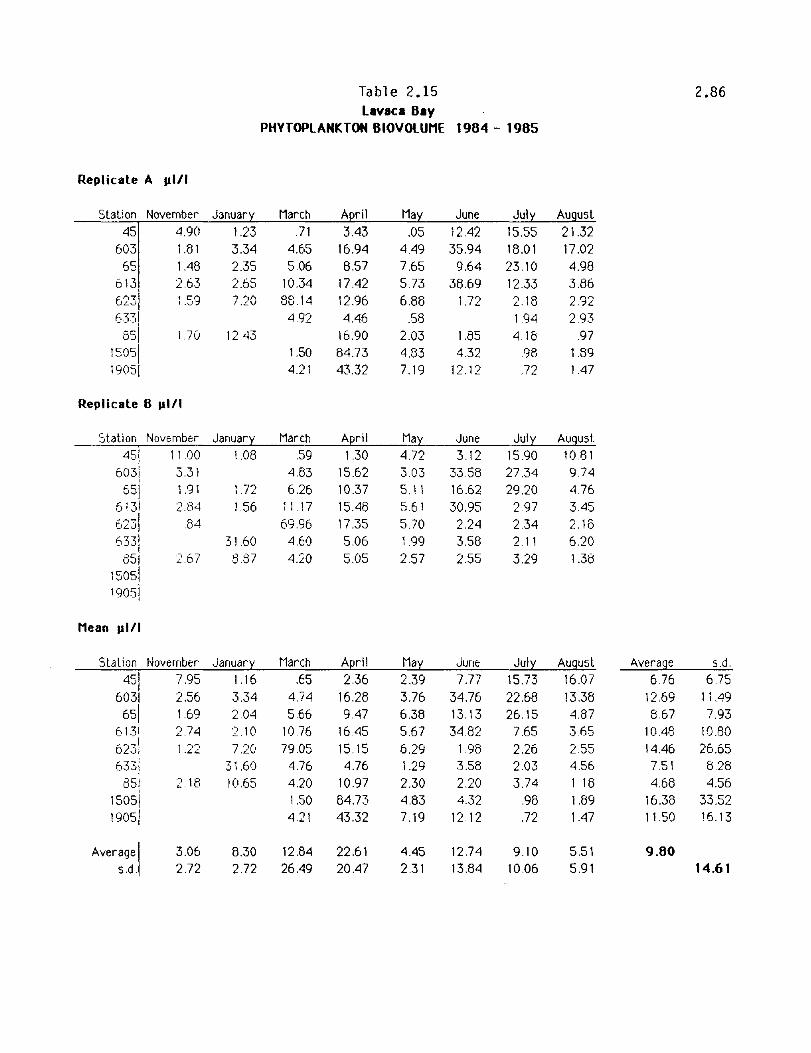
Replicate A JIll I

Station November Januar 45 4.90 1.23

603 1.81 3.34 65 1.48 2.35

613 2.63 2.65

623 i 1.59 7.20

6.33! 851 1.70 12.43

15051

1905!

Replicate 8 JIll I

Station November January I

451

1100 1.08 603

1

3.31

65 1.91 1.72 613 2.84 1.56 6,,-1

LJI 84 633! 31.60

851 2.67 8.87 1505

1 1905

Mean JlI/I

Stalion November Janudl'y 4"1 7.95 1.16 "I

6031 2.56 3.34

651 1.69 2.04 6131 274 210

6231 1.22 720 633( 31.60

I 851 2 18 10.65

15051 19051

Average I 3.06 8.30 s,d. 2.72 2.72

Table 2.15 Lavaca Bay

PHYTOPLANKTON BIOVOLUME 1964 - 1965

March June Jul 71 12.42 15.55

4.65 16.94 4.49 35.94 18.01 5.06 8.57 7.65 9.64 23.10

10.34 17.42 5.73 38.69 12.33 88.14 12.96 6.88 1.72 2.18

4.92 4.46 .58 1.94 16.90 2.03 1.85 4.18

1.50 84.73 4.83 4.32 .98 4.21 43.32 7.19 12.12 .72

March April May June July .59 1.30 4.72 3.12 15.90

4.83 15.62 3.03 33.58 27.34 6.26 10.37 5.11 16.62 29.20

11.17 15.48 5.61 30.95 2.97 69.96 17.35 5.70 2.24 2.34

4.60 5.06 1.99 3.58 2.11 4.20 5.05 2.57 2.55 3.29

March AQril May June Julv .65 2.36 2.39 7.77 15.73

4.74 16.28 3.76 34.76 22.68 566 9.47 6.38 13.13 26,15

1076 16.45 5.67 34.82 7.65 79.05 15.15 6.29 1.98 2.26

4.76 4.76 1.29 3.58 2.03 4.20 10.97 2.30 2.20 3.74 1.50 84.73 4.83 4.32 .98 4.21 43.32 7.19 12,12 ,72

12.84 22.61 4.45 12.74 9.10 26.49 20.47 2.31 13.84 10.06

2.86

17.02 4.98

3.86 2.92 2.93

.97 1.89 1.47

August 10.81 9.74

4.76 3.45 2.16

6.20

1.38

August Average S.d. 16.07 6.76 6.75

13.38 12.69 11.49 4.87 8.67 7.93 3.65 10.48 10,80

2.55 14.46 26.65 4,56 7.51 8.28 1 18 4.68 4.56 1.89 16.38 33.52 1.47 11.50 16.13

5,51 9.80 5.91 14.61

Table 2.16 2.87

lavaca Bay Salinity 1985 - 1986

(Pratical Salinily from Hydrolab Conductivity)

Replicate A. ppt

Station October December F ebruar June Au usl 45 4.7 .8 5.3 13.4 .5 3.9

I 603' 9.9 1.1 8.7 17.1 7.5 3.9

65 69 1.4 8.7 17. ! 1.0 9.4 613 15.9 4.9 13.6 20.8 16.4 10.9

6rl7 "::· .. 11 19.6 8.1 10.6 24.2 20 1 9.6

633j 15.2 6.0 6.2 23.2 19.1 0.7 851 20.8 8.0 13.1 23.9 19.1 10.9

15051

28.9 18.8 14.4 27.7 26.7 23.9

1905, 29.1 20.4 18.0 28.4 26.7 26.0

Replicate B. ppL

Statiorl October December February Apr:l June AUQusl 451 i~. ! .9 ' 7" . .of ~ 3.9 . . J . ..., .,

6031 9.9 1 1 17.4 77 39 55i 6.9 ' . ,<; , 1.0 94 '.4 I ...... , ,

6d 16.3 4.9 211 16.4 10.9 6231 19.8 8 1 24.2 20.4 9.9 , 633' 16.7 0.5 23.2 19.2 9.0

851

20.2 6.3 23.9 18.7 11.2 1505r 28.4 18.5 14 28.1 26.7 24.6

19051 29.3 20.1 18 26.4 27.~ 26.3

Mean. ppt

Slation Oclober December Februar April June Au ust Average s.d. 45 4.4 .9 5.3 13.4 .6 3.9 4.31 4.66

603 9.9 1.1 8.7 17.2 7.6 3.9 7.37 5.76

651 6.9 1.4 8.7 16.1 1.0 9.4 652 5.74

613i 16.1 4.9 13.6 20.9 16.4 10.9 i 2.67 0.56

623 19.7 6.1 10.6 24.2 20.3 9.8 1455 7.76

633 16.0 8.3 6.2 23.2 19.1 8.9 1309 7.36

85 20.5 6.2 13.1 23.9 lB.9 11.0 11.81 7.40 1505 28.7 16.7 14.4 27.9 26.7 24.2 23.41 5.45

19051 29.2 20.3 18.2 28.4 no 26.1 24.B7 4.34

Average I 16.82 7.97 7.29 21.70 15.29 12.01 13.51 s.d. 8.52 7.00 6.88 5.06 9.70 7.70 9.00

Table 2.17 2.88

lavaca Bay WATER TEMPERATURE 1965 - 1966

Replicate A 'C

Station Oc Lober December F ebruar June Au usL 45 26.1 12.B 20.0 27.8 30.0

603 25.7 11.3 21.0 26.0 28.4 30.5

651

27.2 12.5 21.0 25.5 28.0 29.6 613 26.8 10.0 20.4 26.5 28.6 29.7

6231 26.6 10.5 21.0 26.0 28.7 29.2

6331

25.3 10.2 20.5 24.5 28.5 26.6 851 , 25.0 10.6 20.0 24.5 27.4 28.2

1505

1

25.5 12.7 18.5 21.7 27.6 28.0 1905 25.6 13.0 16.8 22.0 28.0 27.0

Replicate B. 'C

SLation OcLober December February A I'il June Au ust A" 26.3 12.5 25.5 28.0 30.0 -,...,

603! 26.5 11.2 26.0 28.6 305 0::.:: ! 27.' 1"', c::. U'-'~ I~.·-, 25.5 28.0 ")(", '?

... :;,1

6 ~3! 26.7 !O.O 26.5 28.7 30.0 I

62.31 26.7 105 26.5 28.7 29.3 . --I '~L :j j 0.4 24.5 25.6 28.7 O,)j' L .• ) .L.

851 25.3 10.6 24.5 27.4 26.2

1505\ 25.5 12.5 19.0 21.8 28.0 28.8 1905j 25.6 12.6 18.4 22.0 28.2 26.7

Mean. 'C

Slation Oclober December F ebruar April June Au usl Average S.d. 45 26.2 12.7 20.0 25.5 27.9 30.0 24.0 6.2

603 26.1 11.3 21.0 26.0 28.5 30.5 24.2 6.9 65 27.2 12.5 21.0 25.5 28.0 29.7 24.2 6.3

613 26.8 10.0 20.4 26.5 28.7 29.9 24.0 7.4 623 26.8 10.5 21.0 26.3 28.7 29.3 24.0 7.1

633 25.3 10.3 20.5 24.5 28.6 28.7 .... 17 ') LJ,L.,

~ ~

'..J.e 85 25.2 10.6 20.0 24.5 27.4 28.2 22.9 6.5

1505 25.5 12.6 18.8 21.8 27.9 28.4 22.5 5.8 1905 25.6 12.8 18.6 22.0 28.1 27.9 22.5 5.7

Average I 26.1 11.5 19.9 24.7 28.2 29.2 23.5 S.d. .7 1.1 1.0 1.7 .4 .9 6.3

Table 2.18 2.89

lavaca Oay SECCHI DEPTH 1965 - 1986

Replicate A. em

Slation October December Februar June Au usl 45 67 35 54 50 50

6031 50 35 52 62 50 34 651 65 34 60 64 51 46

6131

60 44 78 45 45 42 6231 64 39 45 18 62 26 6331 71 44 50 40 66 19

851 67 36 66 SO 60 34 15051 92 80 32 50 45

r

1905 1 91 35 47 43

Replicate B. em

StallOn October December February April June August 451 65 36 7" 47 ,~9 , ,J

6031 46 28 65 51 3; '51 ~ I 6.::1 33 6,Q 4:- ~7

6131 64 44 ·'-15 45 '~2

6231 51 41 28 54 21

633! 66 45 45 54 22 85! 66 41 40 63 37

1505\ 90 19 45 19051 37 45

Mean. em

Slalion Oclober December Februar April June Au ust Average s,d, 45 66 36 84 78 49 50 58,0 17,1

603 48 32 52 64 51 33 45,8 12,3 651 65 34 60 64 50 47 52.4 11.9

'" ,-I - ,,) I 52 411 76 /]7 17 ,::'~ ;L 50,9 i :.5 6231 58 40 45 23 58 24 40,8 16,1 ':'771 UJ..Jj 69 45 80 4::. 60 21 50,2 i 9.5 55 67 39 66 45 62 36 50,9 13,6

1505 91 80 26 50 45 56,6 27,4 1905, 91 36 47 44 49.7 20.8

Average I 67.0 38.2 68.1 47.1 52,9 37.7 50.4

s.d, 13.3 5.1 14.6 18.1 6.4 10.1 16.7

Repliute A

Slation 45

603 65

6131 623

633

1 85

1505

1 1905

Replicate B

Station 45!

603i 6cl

JI , 6t3! . .-. .... 1 I)L.)I - --I b-J-JI

551 15051 19051

Mean

Station 451

6031 65

1 613 623

1

6331

851

15051 , 19051

Averagel S.d.

Table 2.19

lavau Bay pH 1985 - 1986

Oclober December f ebruar 7.5 5. 1 8.6 8.2 8.3 8.5 8.2 6.2 8.5 8.3 5.3 8.5 5.5 5.2 8.2 8.4 8.3 8.1 5.0 8.4 5.5 8.0 8.2 8.3 8.4 8.2 5.2 64 6.6 6.3 5.3 5.<1 5.2 B.3

October December F ebruar:t: April 7.7 8.1 8.4 8.2 8.3 8.3 8.2 8.2 0,3' B.3 8.4 6.2 8.2 8.4 ~ "

o.~

8.0 6.4 B.O 5.2 8.4 5.2

8.4 5.5 5.3 6.4 8.6 5.3

October December f ebruar'( Agril 7.8 B.l 6.6 84 5.2 8.3 8.5 5.3 8.2 8.2 8.5 8.3 5.3 5.4 5.5 5.2 8.2 8.4 8.3 8.1 5.0 6.4 6.5 5.0 5.2 5.4 5.4 5.2 5.2 8.4 8.6 8.3 6.3 5.4 8.4 8.3

8.13 8.32 8.48 8.23 .17 .11 .16 .12

2.90

June Au usl 8.0 5.7 8.4 8.8 7.6 8.6 5. 1 8.6 8.1 7.9 0.1 8.1 8.1 8.5 8.0 e.l

June August B.O 8.7 8.4 B.8 7.6 8.6 6.1 8.6 8.1 7.8 B') 7 r· .';)

8.2 5.5 B.O 5. 1

June August Average S.d. B.O 8.7 8.23 .35 8.4 8.8 8.39 .22 7.6 8.6 8.19 .34 5.1 5.6 5.33 .17 8.1 7.9 8.15 .19 S.1 8.0 8.13 .21 e.l e.5 5.29 .13 8.0 8.31 .23 8.1 8.28 .18

8.05 842 8.25 .20 .35 .24

Table 2.20

Lavan Bay DISSOlVED OXYGEN 1965 - 1966

Replicate A. mgt I

Station October December February AQril June August

6~;1 9.7 9.9 9.5 9.5 B.2 7.4 10.2 10.5 9.7 9.1 8.4 8.7

651 12.0 10.2 9.B 8.9 8.2 8.0

6131 10.6 11. 1 7.5 9.2 10.3 6.7 623

1 8.7 111 90 9.0 7.4 7 1

6331

SA 11.2 q~ 6.3 7.3 7.b _ .L

85. 8.3 11.3 B.8 8.2 7.B 7.5

15051

7.6 10.7 9.0 8.3 7.8 7.5 1905, 7.7 10.5 B.B B.O 79 6.7

Replicate B, mg/l

Station October December February April June August 451 9.5 9.8 9.5 0.2 7.7

6031 10.2 10.7 8.5 8.8 8° .U --I ; 2.2 10.2 3.0 6.5 7.7 D::JI

613i 10.4 " ro, 1 •• L B.9 10.4 5.7

623i 10.2 11.1 89 7.5 7.3 f-- i _I,)·.JI B.6 109 8.1 7.5 7.4 85

1

8.2 10.6 8.7 7.9 7.5 1505 8.3 11.2 8.6 8.2 7.8 7" ..... J

19051 ' ~ 1 A " G.B B.l ' , 0.7 I.' . V.'1 1.4-!

Mean, mg/l

Slation October December Februari: A~ril June August

6~;1 9.6 99 9.5 9.5 8.2 75 10.2 10.6 9.7 8.8 6.6 8.8

65! 12.1 10.2 9.8 B.9 B.4 7.9 613 10.5 11.2 7.5 9.1 lOA 8.7 623 9.4 11.1 9.0 8.9 7.4 7.2 633 8.5 11. 1 9.2 8.2 7.4 7.5

85 B.3 11.0 B.B 8.4 7.8 7.5 1505 8.0 10.9 8.8 8.3 7.8 7.5 1905 7.8 10.5 8.8 8.0 7.6 6.7

Averagel 9.37 10.69 8.98 8.67 8.17 7.69 s.d. 1.40 .47 .62 .49 .89 .66

2.91

Average S.d. p n r • U.::10 .93 9.41 .86 9.50 1.53 9.73 118 8.83 1.46 8.59 1.34 B.61 1.25 8.54 1.21 8.23 1.23

6.93 1.26

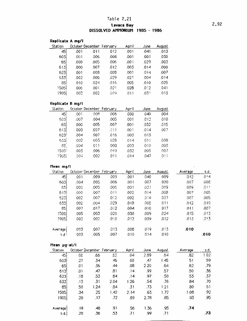
Table 2.21 llvlcI81Y 2.92

DISSOl VEO AMMONIUM 1985 - 1986

Replicate A mgll Station Dc tober December F ebruar June Au ust

45 .001 .011 .012 .041 .013

603 .001 .006 .008 .001 .001 .030

65 .000 ,005 .006 ,001 ,029 ,003

613 ,000 ,007 ,012 ,003 ,014 ,008

623 .001 ,008 .008 ,001 .014 ,007

6331

,002 ,006 ,029 ,021 .004 ,014

351 .010 ,024 ,016 ,005 ,OiD ,025

1505i ,006 ,001 0'01 . "'. ,028 ,012 .041

1905i .002 ,002 .009 .011 .0.31 .013

Replicate 8 mgtl Station October December Februar:z: April June August

451 .001 008 .006 000 040 ,004 .,.) .007 ,004 ,005 .001 .012 .010 b'vji

65

1

000 005 ,007 ,001 .032 ,015

613 ,000 .007 .:J 11 ,001 ,014 ,007

6231 .004 ,007 .016 ,003 ,013

633: 002 003 ,023 .014 .01 i ,008

85( ,004 0; 1 ,008 ,00·3 .010 .008

1505: .003 ,006 .('19 .032 ,OO!;, 007

19051 .004 002 ,Oil ,014 .047 .011

Meln mg/l Station October December F ebruar::r: A~ril June Auaust Average 5,d,

451 ,001 ,009 ,009 ,001 040 ,009 .012 .014 I

6031 ,004 ,005 ,006 001 .007 ,020 .007 ,003

651 ,000 ,005 ,006 ,001 .031 .009 ,009 .OT!

6131 ,000 .007 ,01 I .002 .014 ,008 .007 .OO:~

6",-i "',) I 002 . 007 ° ,r . ' .L .002 .0 1 ~ 007 .007 .005

633i .002 ,004 ,029 .018 005 ,011 ,012 .010

851 ,007 ,017 ,012 ,004 ,1)10 ,017 .011 ,007

1505i ,005 ,003 .020 ,030 ,009 ,024 .015 ,01;:,

19051 ,003 ,002 ,010 ,012 ,039 ,012 ,013 .013

Average I ,003 ,007 .013 ,008 .019 ,013 .010 sdi 003 ,005 ,007 ,0iD ,014 ,010 .010

Mean Ilg-itli StatIOn October December Februar:z: April June AUQusl Average s.d,

45: 06 ,66 t:.') ,04 2,89 .64 .82 1.02 ,u~

6031 ,27 .34 .46 .08 .47 1.45 51 .59

65 ,01 .36 .44 ,08 2.20 ,64 .62 ,79

613 ,01 ,47 ,81 ,14 .99 ,57 .50 ,36

623 ,18 .53 .84 ,14 ,97 ,50 ,53 ,37

633

1

.13 .31 204 1.26 .54 .76 .84 70

85 ,50 1.24 ,84 ,31 ,73 1.21 .80 .51

15051 ,34 .25 1.42 2.14 ,63 1.72 1.08 .92

19051 .20 ,17 .72 ,69 2,78 ,85 .93 ,95

Average I .19 .48 ,91 .56 1.36 ,95 .74 s,d,1 ,20 ,36 .53 ,71 ,99 ,71 .1~

Table 2.22 lavaca Bay 2.93

DISSOlVED NITRITE 1985 - 1986

Replicate A mg/l Station October December Februar June Au ust

45 .003 .002 .000 .004 .001 603 000 .002 .000 000 001 .001

65 .000 .001 .000 .000 .004 .001 613 .000 .001 000 000 .000 .000 623 .000 .000 .000 000 .000 .001 633

1

.001 .000 .000 .002 .000 .O() 1

85 .000 .001 .00 I 000 000 .00i 1505

1

000 .000 .001 .001 001 .001 )905 .000 .001 .000 .001 .001 .001

Replicate IS mg/l Station October December Februarx: AEril June August

451 003 .002 .000 000 .003 .001

6031 .001 .002 .000 000 .001 .001 65\ .000 .002 .000 .000 .004 .001

613l , 000 .000 .001 .000 000 .000 623i 000 .000 000 000 .000 .001 '731 0...; ; .001 000 .001 .001 .000 .001

55j 000 .000 .000 .000 .000 on" . vV

15051 .000 .000 000 .001 .000 001

19051 000 000 .001 .001 002 000

Mean mg/l Station Oclober December Februar June Au usl Average s.d.

45 .003 .002 000 .003 .001 .002 .001 603, .001 .002 ./j00

I 000 .001 .001 .001 .001

651 .000 .001 .000 OO~· .004 .001 .001 .001

613! .000 .001 .000 000 .000 000 .000 000

6231 .000 000 000 000 000 .00 : GOO 000

633i .001 .000 .001 .002 .000 .001 OO~ .OO!

851 .000 .001 .001 .000 000 .000 .000 000

1505

1

.000 .000 000 .001 000 .001 .000 000 1905 .000 .001 .001 1"1.1"1.1 002 .000 .001 .000 .vv 1

Average I .001 .001 .000 .000 .001 .001 .001 s.d. 001 .001 .000 .001 .002 .000 .001

Mun Jlg-atll Station October December Februar June Au ust Average s.d.

45 .19 .17 .02 .24 .05 .11 .10 603 .04 .17 .00 .00 .06 .04 .05 .06

65 .03 .09 .00 .02 .30 04 .08 ,j 1

613 .03 .05 .03 .02 .02 .02 .03 .02 623 .03 .02 .02 .02 .00 .04 .02 .02

633 .05 00 .05 .13 .02 .04 .05 .05

85 .01 .06 .10 .02 .00 .03 .03 .03

1505\ .01 .01 .03 .06 .03 .05 .03 .02

19051 .03 .04 .04 .04 .11 .03 .05 .03

, .05 Average I .05 .07 .02 .03 .09 .04

s.d.) .06 .07 .03 .04 . 11 .01 .06

--~~---

Table 2.23 lavaca Bay 2.94

DISSOLVED NITRATE 1.985 - 1966

Replicate A mgll Station October December Februar June Au ust

45 .172 .226 .001 .136 .008 603 .002 .157 .002 .000 .002

65 .001 .161 .000 .002 .127 .002 613 000 .052 .000 .000 000 .003

6231

000 .028 .001 000 .001 .001 633

1 .063 .002 .005 .011 .001 .002

851

000 .063 .003 .003 .001 .000

15051

000 .005 .003 .010 .002 .001 19051 .000 .019 .001 .009 .003 .003

Replicate 8 mgll Station October December February April June August

45' .172 .222 .003 .000 .143 .001

603 .001 .162 .001 .000 .001 .020

65 .000 .15i .001 .006 .")") • 14.4. .000

6131 000 .043 .001 .001 .001 .001

623! .001 .039 .001 .001 .000 .001

6331 .071 .000 006 O· • . " 000 .002

Bcl '-'I

.000 .037 .002 .005 001 .00 ~

1505j .000 .018 .003 .01 , 001 .00 ;

1905i 001 016- .002 .009 .004 .001

Mean mgll Station October December F ebruar June Au ust Average s.d .

45 . 172 .224 .002 .001 .139 .004 .090 .096

6031 .001 .159 .001 .000 .001 011 .029 .061

65i .001 .156 .001 .004 .124 .oor .048 .069 613i .000 .048 .001 001 .001 .002 .009 .018

6231 .000 .034 .001 000 .001 .001 006 0,7 . ,,-, ~ -71 OJJ, .067 .001 .005 .011 000 .002 .015 .025 851 .000 .050 .003 .004 .001 .001 .010 .020

15051

.000 .011 .003 .010 .001 .001 .005 .005 19051 .000 .017 .002 .009 .004 .002 .006 .006

Averaqe I .027 .078 .002 .00<1 .030 .003 .024 s:di .057 078 .002 .004 056 .005 .052

Mean 119-atll Station Oclober December F ebruarz: April June AUQusl Average S.d.

451 12.26 16.01 .15 .05 9.96 .31 6.46 682 603

1

.09 11.39 .09 .00 .06 .76 2.06 4.37

651 .04 11.13 .08 .29 8.89 .07 3.41 4.92

6131 .02 3.41 .05 .04 .05 .13 .62 1.31 623 .03 2.39 .06 .03 .04 .05 .43 .93

633 4.77 .09 .39 .78 .03 .16 1.04 1.77

85 .02 3.56 .19 .27 .04 .06 .69 1.40

1505 .02 .81 .23 .73 .11 .08 .33 .39

1905 .03 1.23 .13 .61 .25 .12 .40 .44

I 1.92 5.56 .15 1.71 Averagel .31 2.15 .19

S.d. 4.06 5.59 .12 .31 4.01 .32 ~.72

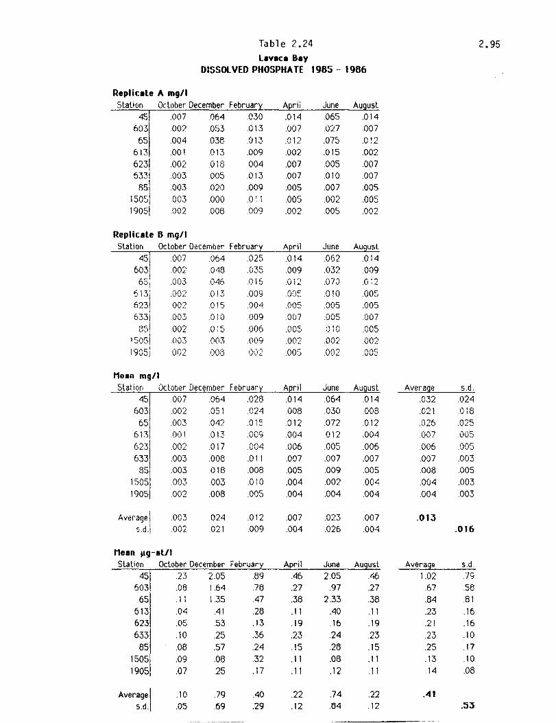
Table 2.24 2.95 lavaca Bay

OISSOL VEO PHOSPHATE 1965 - 1986

Replicate A mgll Station October December Februar June Au ust

45 .007 064 .030 .065 .014

603 .002 .053 .013 .007 .027 .007

65 .004 .038 .013 .012 .075 .012

613 .001 .013 .009 .002 .015 .002

6231

.002 .015 .004 .007 .005 .007

6331

.003 .005 .013 .007 .010 .007

851

.003 020 .009 .005 .007 .005

1505, .003 .000 .011 .005 .002 .005

1905! .002 .008 .009 .002 .005 .002

Replicate B mgt I Station October December F ebruar A ril June Au ust

45 .00/ .064 .025 .014 .062 .014

6031

.002 .048 .035 .009 .032 .009

65i .003 .046 .016 .012 .070 .012 ,h, 1 7 ~ .002 .013 .009 .005 .010 .005 ~2~1 002 .015 .004 .005 .005 .005

633i .003 .010 009 .007 .005 .007

851 .002 .Oi~' .006 .005 010 .005 , 15051 .003 .003 .009 .002 .002 .002

1905/ .002 .005 002 .005 .002 005

Mean mgll Station October December F ebruar' June Au usl Average s.d.

45 .007 064 .028 .064 .014 .032 .024

603 .002 .051 .024 .030 .005 .021 .018

65' .003 .042 0'" .012 .072 .012 .026 .025

6131

1,..1

.OO! .013 .009 .004 012 .004 .007 .005 623' .002 .017 .004 .006 .005 .006 .006 .005

633 .003 .003 .011 .007 .007 .007 .007 .003

85 .003 .018 .008 .005 .009 .005 .008 .005

1505i .003 .003 .010 .004 .002 .004 .004 .003

19051 .002 .008 .005 .004 .004 .004 .004 .003

Average I .003 .024 .012 .007 .023 .007 .013 s.d.! .002 .021 .009 .004 .026 .004 .016

Mean Ilg-atll Slation October December F ebruarz April June August Average S.d.

451

.23 2.05 .89 .46 2.05 .46 1.02 .79

6031 .08 1.64 .78 .27 .97 .27 .67 .58

65 .11 1.35 .47 .38 2.33 .38 .84 .81

613 .04 .41 .28 .11 .40 .11 .23 .16

623 .05 .53 .13 .19 .16 .19 .21 .16

633 .10 .25 .36 .23 .24 .23 .23 .10

85 .08 .57 .24 .15 .28 .15 .25 .17

1505

1

.09 .08 .32 .11 .08 .11 .13 .10

1905 .07 .25 .17 .11 .12 .11 .14 .08

Average I .10 .79 .40 .22 .74 .22 .41 S.d. .05 .69 .29 .12 .54 .12 .5~

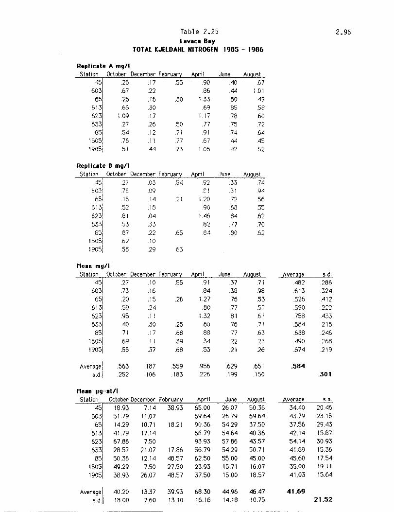
Tabl e 2.25 2.96 llYlca BIY

TOTAL KJElDAHl NITROGEN 1985 - 1986

Replicate A mgll Station October December F ebruar June Au ust

45 .26 .17 .55 .40 .67 603 .67 .22 .86 .44 1.01

65 .25 .16 .30 1.33 .130 .49 613 .65 .30 .69 .85 .58 623 109 .17 1.l7 .713 .60 633 .27 .26 .50 .77 .75 .72

85' .54 .12 .7 i .91 .74 .64

15051 .76 .11 .77 .67 A4 .45 19051 .51 .44 .73 1.05 42 .52

Repllclte B mgll Station October December February April ,June AUQus(

4c ! 27 (F .54 .92 .33 .74 "'I .. '" 6031 .713 .09 ~1 .31 .9<1

651 .15 .14 .21 120 .72 .56 6 pi .52 .16 .90 .68 .55 6~~i .81 .04 1.46 .84 .62 I

6331

.53 .33 .132 .77 .70 13" .137 .22 .65 .84 .50 F.'"

150~1 .v"'

.62 .10 19051 .58 .29 63

Mean mgll Station October December February AQril June August Average s.d.

451 .27 .10 .55 .<) 1 .37 .7 ! .482 .286

603 .73 .16 .84 .38 .98 .613 .324

65\ .20 .15 .26 1.27 .76 .53 .526 .412 6131 .59 .24 .80 .77 c, .590 ')~')

, .. ..I! ..... .:.-623

1

.95 .11 1.32 .81 .6: .753 .433 633 .40 .30 .25 .130 .76 .71 .5134 .215

85 71 .17 .68 .88 .77 .63 .638 .246

15051 .69 .11 39 .34 ,.,~, ·,7 .490 .268 .LL .":;..J

19051 .55 .37 .68 .53 .21 .26 .574 .219

Average I .563 .187 .559 .956 .629 .651 .584 s.dl .252 .106 .183 .226 .199 .150 .301

Meln Jlg-Itll Station October December F ebruar June Au ust AveraQe S.d.

45 18.93 7.14 38.93 26.07 50.36 34.40 20.46 603 51.79 11.07 59.64 26.79 69.64 43.79 23.15

65 14.29 10.71 18.21 90.36 54.29 37.50 37.56 29.43 613 41.79 17.14 56.79 54.64 40.36 42.14 15.87 623 67.86 7.50 93.93 57.86 4357 54.14 30.93

633 28.57 21.07 17.86 56.79 54.29 50.71 41.69 15.36

85 50.36 12.14 48.57 62.50 55.00 45.00 45.60 17.54 1505

1

49.29 7.50 27.50 23.93 15.71 16.07 35.00 19.11

1905 38.93 26.07 48.57 37.50 15.00 18.57 41.03 15.64

Average I 40.20 13.37 39.93 68.30 44.96 46.47 41.69

s.d.1 113.00 7.60 13.10 16.16 14.18 10.75 21.52

------_. - -- ------~------~- ----- --------

Table2.26 2.97 leven Bey

TOT Al PHOSPHATE 1985 - 1986

Replinte A mgt. Slation October December Februar June Au usl

45 .15 .24 .10 .12 .12 603

1

.1~ .26 .11 .13 .11 .13

65 .13 .23 .06 .11 .14 .11

6 131 .10 .16 .08 .11 09 11

6231

.13 . i I .12 .24 .07 .24

6~~1 .10 .13 .07 .17 .06 .17

.09 .18 .07 .17 .07 .17

1505 .10 .07 .07 .18 .11 .18

19051 .09 .11 .10 .22 .10 .22

Replicete 8 mgt. Station October December February April June Auqusl

I 45

1 .18 .25 .10 .11 .12 .11

6031 p .30 .12 .14 .! I .14

6S\

.• J

.16 .27 .10 . i 1 .13 .11

613

1

.10 .15 .09 .11 .08 ' , • j i

623. .12 .13 .14 .26 .07 .26

6331 I

.10 I' .• J 0"· . 1 fj .05 IC' .IU 8"; JI

! 17 . ,~ .18 .06 .1~ .07 14

15051 .10 .06 .06 .28 .08 .28

19051 .10 .10 .10 .26 12 26

Meen mgt. Station October December February A~rii June August Average s.d.

45i .16 24 .10 .11 .12 .11 143 ""') v,-'~~

6031 .14 .28 . i 1 .14 " ., I .14 .151 061

551 I .14 .25 .08 .11 .13 11 .136 .058

6131 .10 16 .08 ' , .09 . i 1 .105 .026 .1 I

623! !~ .,., .13 .25 07 .25 .156 .071

6331

. I "-

10 .13 .06 .17 .05 .17 .116 .05 ! 85, .10 .18 .07 .15 .07 .15 120 .047

1505

1

.10 .06 .07 .23 .10 .23 .132 .OBI 1905 .10 .11 .10 .24 .11 .24 .151 .069

Average I .119 .170 .090 .169 .095 .169 .135 s.d. .025 .071 .024 .060 028 .060 .059

Meen J,lg-ett' Station October December February Aeril JIJne August Average s.d.

6~;1 5.25 7.84 3.22 3.69 4.00 3.69 4.62 1.67

4.36 8.92 3.67 4.38 3.50 4.38 4.87 1.96

65 4.56 B.06 2.70 3.51 4.33 3.51 4.44 1.86

613 3.26 5.07 2.72 3.55 2.77 3.55 3.49 .84

623 4.05 3.95 4.13 8.05 2.26 8.05 5.08 2.30

633

1

3.24 4.31 1.98 5.64 1.73 5.64 3.76 1.65

85 3.31 5.76 2.14 4.93 2.17 4.93 388 1.53

1505

1

3.31 2.08 2.14 7.39 3.13 7.39 4.24 2.60

1905 3.19 3.46 3.28 7.83 3.61 7.83 4.87 2.24

Average I 3.84 5.50 2.89 5.44 3.06 5.44 4.36 S.d. .79 2.30 .77 1.94 .90 1.94 1.91

Table 2.27

Lavaca Bay CHLOROPHYlL a 1985 - 1986

Replicate A JlglI (corrected algorithm)

Station October December Februar .June Au IJst 45 24.55 8.99 14.04 4.69 21.66

603 15.85 14.67 7.92 5.57 11.20 29.16

651 14.95 1 "i .52 9.72 8.45 4.90 13.23 613

1

16.00 12.22 5.97 7.56 11.50 9.85 623 5.31 4.20 28.87 14.15 3.98 5.54

6331 5.02 2.39 4.44 5.32 1.49 10.08 851 10.42 5.80 1.96 11.03 1.50 6.77

1505

1

10.77 5.91 2.88 12.98 957 906 1905 8.14 7.67 6.29 12.14 9.49 10.38

Replicate B Jlgil

StaUon October December February Aoril June Auqust , 45!

I lb.27 11.40 1 1 .5~5 7.59 .j d9 23 t· il

603i 18.33 19.30 r 77 I ,,-'.J 6.:'4 12.75 28.25

6"'; ,~ 'I' 1676 885 945 ... r,-:;: ; 279 v, , 'J , " ~ '.J,-'

6131 13.36 12.24 5.74 7.25 It'.32 10.69 623: 7.9<1 6.88 24.90 13.41 Ll '"'; .. ...... '-) 6.85

6331 5.09 2.59 2.4e 6.98 156 1023 851 2.16 11.28 1.55 9.44

1505

1

806 6.52 "i.85 11.52 10.61 9.03

1905 8.91 7.52 6.59 12.35 9.14 11.10

Mean IIg/ l

Station October December Februarl' April June August 451 20.57 10.20 12.79 7.35 "i59 22.75

6031 17.09 16.99 7.63 5.91 11.97 28.71 , 65 15.56 15.64 9.28 8.95 4.46 i3,O 1

613 14.68 12.23 7.35 7.41 :3.91 10.27

623. 6.63 5.54 26.55 13.78 4.10 6.19

6331 5.05 2.49 3.46 6.15 1.53 10.15 ,

8-' 10.42 5.80 2.06 11.16 1.67 6.10

150~1 9.42 6.21 3.87 12.25 1009 9.05

1905! 8.52 7.59 6.44 12.25 9 7 ') .0-'- 10.74

Average 1 12.09 939 8.86 9.47 6.85 13.22 sal 5.50 4.97 7.36 2.90 4.51 729

2.98

Averaae S.d.

13.0"i 7 r" .L;

14.72 7.98

11.15 4.23

10.97 3.30

10.52 8.38 4.81 .3.02 6 ?? c1.13 8.48 2.96

9.14 2.03

9.96 5.91

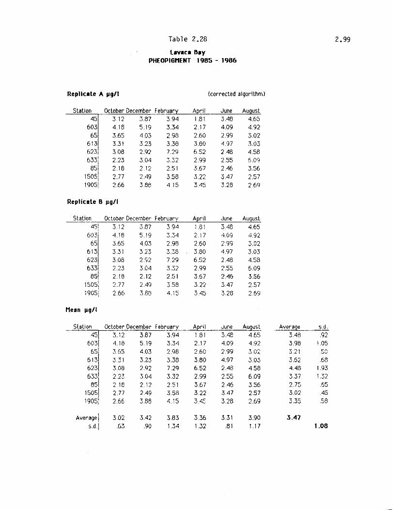
Table 2.28

l.v.n O.y PHEOPIGHENT 1985 - 1986

Repllnte It. IIgll (corrected algori thm)

Station October December F ebruar June August 45 3 12 3.87 3.94 3.48 4.65

603 4.18 5.19 3.34 2.17 4.09 4.92

65 3.65 4.03 2.98 2.60 2.99 3.02 613 3.31 3.23 3.38 3.80 4.97 3.03 623 3.08 2.92 7.29 6.52 2.48 4.58 633: 2.23 3.04 3.32 2.99 2.55 0.09

85 2.18 2 12 2.51 3.67 2.46 3.56 1505 2.77 2.49 3.58 3.22 3.47 2.57 1905 2.66 3.65 4.15 3.45 3.25 2.69

Replicate B IIgll

Station October December February A~ril June August 45! 3.12 3.87 3.94 1.81 3.48 4.65

603; 4.15 5.19 3.3-4 2.17 4.09 4.92

65 3.65 4.03 2.98 2.60 2.99 302 613 3.31 3.23 3.38 3.80 4.97 3.03 623 3.08 2.92 7.29 6.52 2.48 4.58 633

1

2.23 3.04 3.32 2.99 2.55 6.09 85 2.18 2.12 2.51 3.67 2.46 3.56

1505 2.77 2.49 3.58 3.22 3.47 2.57

1905! 2.66 3.06 4.15 3.45 3.28 2.69

Me.n IIgll

Station October December F ebruar June Au ust 45 3.12 3.87 3.94 3.48 4.65

603\ 4.18 5.19 3.34 2.17 4.09 4.92

65 3.65 4.03 2.98 2.60 2.99 3.02 613 3.31 3.23 3.36 3.80 4.97 3.03 623 3.08 2.92 7.29 6.52 248 4.58

6331

2.23 3.04 3.32 2.99 2.55 6.09

85 2.18 2.12 2.51 3.67 2.46 3.56

15051 2.77 2.49 3.58 3.22 3.47 2.57

1905j 2.66 3.88 4.15 3.45 3.28 2.69

Average I 3.02 3.42 3.83 3.36 3.31 3.90

s.dl .63 .90 1.34 1.32 .81 1.17

2.99

Average S.d. 3.48 .92 3.98 LOS 3.21 CA

.~V

3.62 .68 4.48 1.93

3.37 1.32 27~, .65 3.02 .45

3.35 .58

3.47 1.08

Table 2029 2.100

Lav.n B.y PHYTOPLANKTON 1985 - 1986

(Note th8t Units for Cell Numbers 8re Celis/ill)

Phytopl.nklon Cell Numbers, celis/pi

Slalion Oclober December F ebruar June Au usl Average s.d. 45 580 510 1240 1490 1210 1052 405

603 247 569 2380 654 3710 2450 1668 1382 65 1230 901 3020 624 1350 9500 2521 3520

613 762 1500 1130 656 948 7730 2121 2764 623 757 611 1390 1040 606 11900 2717 4509 633 259 1190 663 191 1970 9350 2276 3527

85 590 881 933 420 641 13700 2861 5313 1505 125 246 445 255 477 6080 1277 2356 1905 124 309 213 745 825 5610 1304 2129

Average 523 746 1269 655 1335 7537 2011 s.d. 365 411 909 346 1014 4141 30-41

PhyLopl.nklon Biovolume. JlIII

Slation Oclober December Februar June Au usl Average S.d. 45 7.9 11.1 26.5 12.9 6.1 11.4 5.0

603 20.1 4.4 15.9 10.6 7.9 10.6 7.6 65 94.9 6.5 52.2 1.9 1.5 53.5 35.1 35.1

613 20.1 11.6 3.0 1.2 1.5 20.0 9.6 9.0 623 16.0 3.9 6.0 3.3 2.1 32.3 10.6 11.5 633 12.4 14.0 3.0 0.6 6.9 24.6 10.2 5.7 85 16.3 15.9 1.6 1.7 1.4 30.6 11.3 11.5

1505 40.5 2.8 11.2 1.8 4.2 15.5 12.6 14.6 1905 4.5 20.1 3.9 2.5 3.0 19.1 5.5 8.4

Average 25.8 10.1 14.1 2.1 4.9 23.3 13.04 s.d. 27.8 6.0 16.6 1.1 4.3 14.5 16.7

Table 2.30 LlIYaca Bay

PHYTOPLANIHON TAXONOMIC COMPOSITION 1965-1966 (an stations combined)

Relative fraction of totel concentration (cellsl ml)

Taxon October December Februar June Au usl Average CYllnophyles .826 .733 .828 .911 .919 .844

Diatoms .006 .003 .009 .001 .001 .000 .003 Chlorophyles .121 .197 .140 .125 .080 .070 .122 Cryplophyles .003 .002 .001 .001 .000 .000 .001

Dinonllgellales .001 .000 .000 .000 .000 .000 .000 Flagellates !Ix Monads .043 .064 .021 .023 .OOB .010 .02B

Monthly relative fraction: .127 .175 .256 .217 .035 .191 1.00

Rel.tive fraction of total biovolume (pI/mil

Taxon October December F ebruar June Au usl Average Cyanophyles .666 .530 .942 .605 .700 .662

Diatoms .106 .199 .021 .098 .168 .030 .104 Chlorophyles .034 .094 .011 .087 .062 .051 .057 Cryptophyles .003 .014 .002 .017 .010 .005 .009

Dinonagellales .159 .017 .014 .122 .059 .009 .063 Flagellales !Ix Monads .033 .143 .009 .146 .092 .201 .104

Monthly relative fraclion: .208 .077 .454 .031 .031 .200 1.00

2.101

John Cullen 2124/67

Table 2.31

Light-limitation Modol

(photosynthesis Model from Platt et a1. 1960. J. Mar. Res. 36: 667-701)

Model of photosynthesis: Pi = Ps*(1 - exp«-a*1)/Ps»*exp«-b*1)/Ps) Definition of saturating light: Is = Ps/a

Scaling of photosynthesis: P' = PUPs Scaling of light: r = Ills

SCllling of IIttenulltion coefficient: k' = k/z where z is depth of the well-mixed Illyer Scaled Photosynthesis equation: P' = (I - exp(-r»*exp«-b*r)/a)

6 April 1966 1200 h water column avg. Ps 23.95 from MA thesis alpha .072 of R.F. Davis: beta .0034

15 333 jJmollm'2/s 10 566 Jlmol/m'2/s (cloudy) k 2.4 m'-I

water depth 1.7 m k' 1.41 r 1.76

Table of relative photosynthesis in a mixed layer as a function of incident light and water clarity

Across: Extinction coefficient t:. (water column depth = I" light depth when It' = ".61)

Down: " = lolls (Incident light/Saturating light)

Correeling for Respiration. Relative to Roference Rate from Sampling Date

It' --)

r .5 1.0 1.5 2.0 4.0 6.0 10.0 20.0 40.0 .5 .55 .41 .30 .22 .02 -.07 -.14 -.19 -.22

1.0 1.07 .87 .71 .57 .23 .08 -.05 -.15 -.20 1.5 1.39 1.191 1.001 .83 .39 .19 .01 -.12 -.18 2.0 1.60 1.41 1.21 1.03 .53 .26 .07 -.09 -.17 4.0 1.82 1.76 1.63 1.47 .86 .52 .21 -.02 -.14 6.0 1.62 1.71 1.73 1.68 1.15 .73 .34 .04 -.11

10.0 1.49 1.62 1.69 1.66 1.22 .79 .36 .06 -.10 15.0 1.20 1.38 1.51 1.58 1.31 .88 .44 .09 -.09 20.0 .96 1.16 1.33 1.45 1.34 .93 .47 .10 -.08

The outlined cell represents the approximate conditions midday on the day of sampling.

Water column photosynthesis is clearly sensitive to incident light and water clarity.

l VDlIgIllTaDleAproo

2.102

Table 2.31 (cant.) 2.~=3

Llght-LlmltaUon Model

lavaca 8ay April 1986

Correcting for Respiration = Pmax· .1

t" --)

," .5 1.0 1.5 2.0 4.0 6.0 10.0 20.0 40.0 .5 .22 .16 .12 .09 .01 -.03 -.06 -.08 -.09

1.0 .42 .35 .28 .22 .09 .03 -.02 -.06 -.08 1.5 .55 .471 .401 .33 .16 .07 .01 -.05 -.07 2.0 .63 .56 .48 .41 .21 .11 .03 -.04 -.07 4.0 .72 .70 .65 .58 .34 .20 .08 -.01 -.06 8.0 .64 .68 .69 .66 .45 .29 .14 .02 -.04

10.0 .59 .64 .67 .66 .48 .31 .15 .02 -.04 15.0 .47 .54 .60 .63 .52 .35 .17 .04 -.03

20.0 .38 .46 .52 .57 .53 .37 .18 .04 -.03

Re'ative Rate of Gross Photosynthesis - Maximum = 1.0

0.5 1 1.5 2 4 6 10 20 40 0.5 .32 .26 .22 .19 . 11 .07 .04 .02 .01

.52 .45 .38 .32 .19 .13 .08 .04 .02 1.5 .65 .571 .501 .43 .26 .17 .11 .05 .03

2 .73 .66 .58 .51 .31 .21 .13 .06 .03 4 .82 .80 .75 .68 .44 .30 .18 .09 .04 8 .74 .78 .79 .76 .55 .39 .24 .12 .06

10 .69 .74 .77 .76 .58 .41 .25 .12 .06 15 .57 .64 .70 .73 .62 .45 .27 .14 .07 20 .48 .56 .62 .67 .63 .47 .28 .14 .07

L V811ghLTableApr86

John Cullen 2124/67

Table 2.32

lighl-limilalion Modal

(photosynthesis Model from Platt et III. 1960. J. Mllr. Res. 36: 667-701)

Model of photosynthesis: Pi = Ps" (1 - expel -a" IJ/Ps»"exp« -b" 1)/Ps) Definition of saturating light: Is = Psla

Scaling of photosynthesis: P' = Pi IPs Scaling of light: r = Ills

Scaling of attenuation coefficient: k' = k/z where z is depth of the well-mixed layer Scaled Photosynthesis equation: P' = (1 - exp(-I'l)"exp«-b"l'l/a)

4 June 1966 1200 h waler column avg. Ps 12.72 from MA thesis alpha .059 of RJ. Davis: bela .0013

Is 216 Jlmol/mA2/s 10 1766 IImol/mA2/s (cloudy) k 2.0 mA-l

water depth 1.7 m k' 1.16 I' 6.20

Table of relative photosynthesis in a mixed layer 115 • function of incident light and wllter clarity

Across: Extinction coefficient t'. (wilier column depth = '" light depth when k' = 4.61)

Down: I' = 10115 (Incident Iight/Saturating ligh t)

Correcting for Respiralion. Relalive lo Reference Rale from Sampling Date

t' --)

" .5 1.0 1.5 2.0 4.0 6.0 10.0 20.0 40.0

.5 .26 .21 .16 .11 .01 -.03 -.07 -.10 -.11

1.0 .55 .45 .36 .29 .12 .04 -.03 -.06 -.10

2.0 .84 .74 .64 .54 .27 .15 .04 -.04 -.08

4.0 1.01 .96 .66 .79 .46 .28 .12 -.01 -.07

6.0 1.01 1.00 .96 .89 .56 .35 .16 .02 -.06

8.0 .981 1.001 .99 .94 .63 .40 .19 .03 -.05 10.0 .95 .98 .99 .96 .68 .44 .22 .04 -.04 15.0 .86 .91 .95 .96 .75 .50 .26 .06 -.03

20.0 .78 .84 .89 .92 .79 .54 .28 .08 -.03

The outlined cell represents the approximate conditions midday on the day of sampling.

Water column photosynthesis is near mllximlll for the likely range of incident light and water clarity.

L VBLightTableJun86 2124/87

2.104

Table 2.32 (Cont.) 2.105

Light-llmll.Uon Model

Correcting for Resplr.Uon = Pmu- .1

t' --) I' .5 1.0 1.5 2.0 4.0 6.0 10.0 20.0 40.0

.5 .22 .17 .12 .09 .01 -.03 -.06 -.08 -.09 1.0 .43 .35 .29 .23 .09 .03 -.02 -.06 -.08 2.0 .66 .58 .50 .42 .21 .12 .03 -.03 -.07 4.0 .79 .75 .69 .61 .36 .22 .09 .00 -.05 6.0 .79 .79 .75 .70 .44 .27 .13 .01 -.04 8.0 .77 .78 .77 .74 .49 .31 .15 .02 -.04

10.0 .74 .77 .77 .75 .53 .34 .17 .03 -.03 15.0 .67 .71 .74 .75 .59 .39 .20 .05 -.03

20.0 .61 .66 .70 .72 .62 .42 .22 .06 -.02

Rel.Uve R.te of Gross Photosynthesis - Muimum = 1.0

0.5 I 1.5 2 4 6 10 20 40 0.5 .32 .27 .22 .19 .11 .07 .04 .02 .01

1 .53 .45 .39 .33 .19 .13 .08 .04 .02 2 .76 .68 .60 .52 .31 .22 .13 .07 .03 4 .89 .85 .79 .71 .46 .32 .19 .10 .05 6 .89 .89 .85 .60 .54 .37 .23 .11 .06 8 .671 .661 .67 .84 .59 .41 .25 .12 .06

10 .84 .87 .87 .85 .63 .44 .27 .13 .07 15 .77 .61 .84 .85 .69 .49 .30 .15 .07 20 .71 .76 .80 .82 .72 .52 .32 .16 .08

l VDugnlTlIDleJunoo 212""07

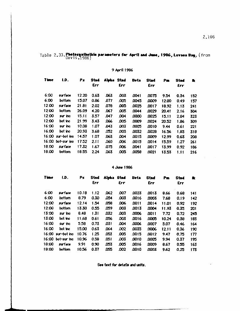
2.106

Tabl e 2.33.PM~"~"tHtto , .. MMt.,.S fer AtwfI aM ..... 1986. Ln ... Bat, (from Davls, 986

9 Apr111986

Tim. I.D. Ps stu AlpM StU B.t. Stad Pm Stll4l Ie Err Err Err Err

6:00 N'f_ 12.20 0.63 .063 .003 0041 .0075 9.54 0.34 152 6:00 bottom 15.07 0.86 .on .005 .0045 .0009 12.00 0.49 157 12 :00 surf_ 21.81 2.Q2 .078 Jm .~ .0017 18.92 1.13 241 12:00 bottom 26.09 4.20 IJ67 .D05 .0044 .0029 20.41 2.16 304 12:00 sur inc 15.11 3.57 .047 004 .0000 .0025 15.11 2.84 323 12:00 botm 21.99 3.43 .066 .D05 .0009 0024 20.52 1.86 309 16:00 sur inc 10.08 1.07 .043 .D03 .ooos .0010 9.44 0.61 221 16:00 botm 20.93 3.68 .052 .003 .0032 .0028 16.56 1.83 318 16:00 N'-bot inc 14.57 1.07 .063 004 .0015 .0009 12.99 0.63 208 16:00 bot-slr m 17.52 2.11 .060 .006 .0015 .0014 15.59 1.27 261 18:00 surfiCf 17.32 1.67 .075 .006 0041 .0017 13.99 0.92 186 18:00 bottom 18.55 2.24 .063 .005 .0058 .0021 13.53 1.11 216

4 Joot 1986

TicH I.D. Ps SWI AI",. Stad B.t. StH Pm Stad • Err Err Err Err

6:00 surf_ 10.18 1.12 .062 .007 .0023 .0013 8.66 0.68 141 6:00 bottom 8.79 0.30 .D54 .003 .0016 .()()()3 7.68 0.19 142 12:00 surf_ 12.14 1.54 .058 .006 .0011 .0014 11.01 0.92 192 12:00 bottom 13.30 0.55 .059 .D03 .0013 .QOO4 11.93 0.35 201 13:00 sur inc 8.48 1.31 .Q32 .D03 .QOO6 .0011 7.72 0.72 245 13:00 botm 11.68 0.61 .056 .Q03 .0016 .0005 10.24 0.38 183 16:00 sur inc 5.58 0.73 .031 004 .QOO6 .0007 5.07 0.46 164 16:00 bot inc 15.00 0.63 IJ64 .D02 .Q035 .0006 12.11 0.36 190 1 6:00 sur-bot inc 10.76 1.25 .053 .005 .0015 .0012 9.47 0.75 In 16:00 bot-sur m 10.96 0.58 .051 .003 .0010 .0005 9.94 0.37 195 18:00 surf_ 9.91 0.90 .053 .D05 .0016 .0009 8.67 0.55 163 18:00 bottom 10.56 0.37 .055 .D02 .0010 0003 9.62 0.25 173

s.. t.xt for ct.Ufls Ind 1Ilfts.

CHAPTER 3

BENTHIC RESPIRATION RATE AND AMMONIUM FLUX

INTRODUCTION

3.1

Benthic nutrient regeneration provides a significant proportion of

inorganic nutrients for primary production III shallow marine environments

(Fisher et al. 1982, Nixon and Pilson 1983, Boynton and Kemp 1985). The

potential for nutrient regeneration III sediments is primarily dependent upon

deposition of organic matter from the water column. Estuarine sediments

with higher organic content support higher microbial metabolism (Waksman and

Hotchkiss 1938) and result in more regeneration of inorganic nutrients (Seki et

al. 1968, Aller and Yingst 1980). Nixon and Pilson (1983) reported that the

benthic remineralization of a marine environment was closely related to the

primary production plus organic input into that area. Therefore, higher

primary production in the water column may result in more nutrient flux from

sediments in an estuary, unless particulate organic matter in the water column

is substantially flushed out to the open sea.

Freshwater inflow is also an important source of inorganic nutrients for

primary production (Barlow et al. 1963, Sharp 1982, Nixon and Pilson 1983) and

terrestrial organic matter in estuarine environments (Shultz and Calder 1976).

Therefore, it is likely that benthic flux of inorganic nutrients may be affected

by freshwater inflow into an estuarine environment.

However, little information is available about long term effects of

freshwater inflow upon benthic nutrient regeneration in an estuarine

environment. Benthic ammonium flux and oxygen consumption rates were

measured in the Lavaca Bay estuary, Texas, monthly or bimonthly for two

consecutive years. During the study period, freshwater inflow into the estuary

3.2

was much greater for Year 1 (November 1984-August 1985) than for Year 2

(October 1985-August 1986).

METHODS

Deployment of Chambers

Two opaque fiberglass chambers, A and B (18 liter volume), were deployed

at station 85 to determine benthic respiration and ill situ ammonium flux

across the sediment-water interface. The chambers were set carefully on the

seafloor to minimize disturbance of sediments. An oxygen probe (YSI 5139)

connected to a dissolved oxygen meter was installed only in Chamber A.

Chamber water was circulated by a deck-mounted Masterflex pump (Barnant

Co.) through Tygon tubing (ID 0.63cm, length 2x15m) wrapped with black

electrical tape to exclude light. Chamber water was sampled whenever desired,

via a two-way valve connected to the outlet of the Masterflex pump.

Circulation of water within the chamber was gentle enough not to disturb the

surface sediment inside of the chamber.

chamber via tubing was about 0.5 hour.

Benthic Respiration Rate

The turnover time of water in the

Benthic respiration rate was determined by measuring the dissolved

oxygen concentration in the chamber water through time and correcting for

water volume and chamber area. Since chemical oxygen demand was not

determined, these respiration rates are really total oxygen demand (Dale, 1978).

The concentration of dissolved oxygen was measured by both the Winkler

method and with a polarographic electrode (chamber A), or only by the

Winkler method (chamber B). Before each experiment, the dissolved oxygen

3.3

meter was calibrated by comparison with Winkler determinations on identical

samples of bottom water. During each experiment (about 4 hours), triplicate

20 ml samples of the chamber water were collected and fixed every 40-50

minutes for titration. The first sample of chamber water was not collected

until at least 30 minutes after setting the chambers because oxygen was

rapidly consumed at the onset presumably due to disturbance of sediments. All

Winkler titrations were completed within two hours of sampling.

Ammonium Analysis of Sediment Pore Water

Sediment cores were sampled with a core sampler (ID 6.5 cm, height 25

cm) without disturbing textures of the sediment from seven stations in the

Lavaca Bay estuary. Sediment cores were sectioned at I cm intervals over the

top 10 cm. Sectioning at I cm intervals was judged to be appropriate because

0.5 ml, the minimum amount of pore water for ammonium assay, was extracted

from each section. Each section was put into a sterile plastic petri dish which

was then sealed with black electrical tape to avoid any loss of pore water.

Replicate samples were frozen immediately and were kept frozen until analyzed.

Pore water from each sediment section was extracted by centrifugation (5000 x

g). Ammonium concentration was determined colorimetrically (Solorzano 1969)

using a spectrophotometer (Beckman Model 24).

Ammonium Flux

Benthic ammonium flux across the sediment-water interface was

determined in two ways. At station 85 the change in ammonium concentration

of chamber water was measured in situ. Chamber water samples were filtered

through glass fiber filters (GF IF) and were kept frozen until analyzed.

3.4

Theoretical ammonium flux (calculated ammonium flux) of each station was

independently calculated from the profile of ammonium concentrations in

sediment pore waters. The theoretical calculation is based on Fick's first law,

and the following equations were used (Klump and Martens 1981).

ls = - 00 Ds (a~ pw

ls = flux of ammonium across the sediment (/Lg-at N m- 2 hour-I)

00 = porosity at the sediment-water interface (unitless)

Ds = bulk sediment diffusivity (cm2pw.sec- l )

D _ Do s - 0

0F

where

Do = molecular diffusivity of ammonium (cm2 sec-I) (Klump and Martens 1981) pw

F = formation resistivity factor (Ullman and Aller 1982)

I F = - clfor ° ~ 0.7, m = 3; for ° < 0.7, m = 2)

o

(~~ = gradient of ammonium concentration at the sediment-water

pw interface

The gradient was calculated by three different ways as described below. The

method used depended on the pattern of the profile of ammonium concentration

in the sediments.

I) When the ammonium concentration increased linearly with depth into

the sediment, the gradient was obtained from the slope of

concentration versus depth.

2) When ammonium concentration increased exponentially with

sediment depth, the gradient was obtained as follows (Klump and

Martens 1981):

~~C) = a (C - Co) e-az

pw

a = constant

z = depth (cm)

Cz, C ,Co; concentration of ammonium at depths z, infinity and zero

(the sediment-water interface) respectively (Ilg-at N I-I)

3) When the ammonium concentration of the top sediment section

(0-1 cm) was equal to or higher than that of pore water of the next

lower sediment section (1-2 cm), the gradient was calculated using

the following equation:

[NH4+] of the top sediment - [NH4+j of the overlying water

0.5 cm

3.5

This calculation is based on arbitrary assumptions that; (I)

ammonium concentration in the pore water increases linearly with

depth within the upper cm of sediment, and (2) that the

ammonium concentration at the sediment-water interface was

identical to that of overlying water. These assumptions may not be

appropriate III all cases. However, this calculation may provide

relative values of theoretical flux and allow us to compare the flux

at different stations when ammonium concentration is maximal in the

top sediment section.

Porosity of sediments (Table 3.1) was determined using the following equation:

Porosity (0) = water content of sediment/volume of sediment

Water content of the sediment was measured as the difference in weight

between the wet sediment and the dry sediment (dried at 45"C for two weeks).

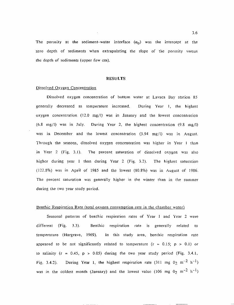
3.6

The porosity at the sediment-water interface (00) was the intercept at the

zero depth of sediments when extrapolating the slope of the porosity versus

the depth of sediments (upper few cm).

RESULTS

Dissolved Oxygen Concentration

Dissolved oxygen concentration of bottom water at Lavaca Bay station 85

generally decreased as temperature increased. During Year I, the highest

oxygen concentration (12.0 mg/l) was in January and the lowest concentration

(6.8 mg/I) was in July. During Year 2, the highest concentration (9.8 mg/l)

was in December and the lowest concentration (5.94 mg/I) was in August.

Through the seasons, dissolved oxygen concentration was higher in Year I than

in Year 2 (Fig. 3.1). The percent saturation of dissolved oxygen was also

higher during year I than during Year 2 (Fig. 3.2). The highest saturation

(122.8%) was in April of 1985 and the lowest (80.8%) was in August of 1986.

The percent saturation was generally higher in the winter than in the summer

during the two year study period.

Benthic Respiration Rate (total oxygen consumption rate in the chamber water)

Seasonal patterns of benthic respiration rates of Year I and Year 2 were

different (Fig. 3.3). Benthic respiration rate is generally related to

temperature (Hargrave, 1969). In this study area, benthic respiration rate

appeared to be not significantly related to temperature (r = 0.15; p > 0.1) or

to salinity (r 0.45, p > 0.05) during the two year study period (Fig. 3.4.1,

Fig. 3.4.2). During Year 1, the highest respiration rate (311 mg 02 m- 2 h -I)

was in the coldest month (January) and the lowest value (106 mg 02 m- 2 h- I)

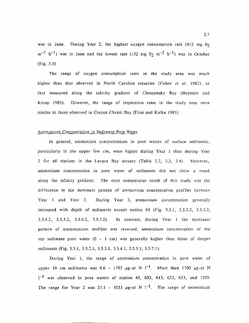
3.7

was In June. During Year 2, the highest oxygen consumption rate (412 mg 02

m-2 h- I ) was in June and the lowest rate (132 mg 02 m- 2 h- I) was in October

(Fig. 3.3).

The range of oxygen consumption rates in the study area was much

higher than that observed in North Carolina estuaries (Fisher et al. 1982), or

that measured along the salinity gradient of Chesapeake Bay (Boynton and

Kemp 1985). However, the range of respiration rates in the study area were

similar to those observed in Corpus Christi Bay (Flint and Kalke 1985).

Ammonium Concentration in Sediment Pore Water

In general, ammonium concentrations in pore waters of surface sediments,

particularly in the upper few cm, were higher during Year I than during Year

2 for all stations in the Lavaca Bay estuary (Table 3.2, 3.3, 3.4). However,

ammonium concentration In pore water of sediments did not show a trend

along the salinity gradient. The most conspicuous result of this study was the

difference in the dominant pattern of ammonium concentration profiles between

Year and Year 2. During Year 2, ammonium concentration generally

increased with depth of sediments except station 65 (Fig. 3.5.1, 3.5.2.2, 3.5.3.2,

3.5.4.2, 3.5.5.2, 3.5.6.2, 3.5.7.2). In contrast, during Year the dominant

pattern of ammmonium profiles was reversed; ammonium concentration of the

top sediment pore water (0 - I cm) was generally higher than those of deeper

sediments (Fig. 3.5.1, 3.5.2.1, 3.5.3.1, 3.5.4.1, 3.5.5.1, 3.5.7.1).

During Year I, the range of ammonium concentration in pore water of

upper 10 cm sediments was 9.6 - 1793 JLg-at N I-I. More than 1700 JLg-at N

I-I was observed in pore waters of station 45, 603, 613, 623, 633, and 1505.

The range for Year 2 was 27.1 - 1033 JLg-at N I-I. The range of ammonium

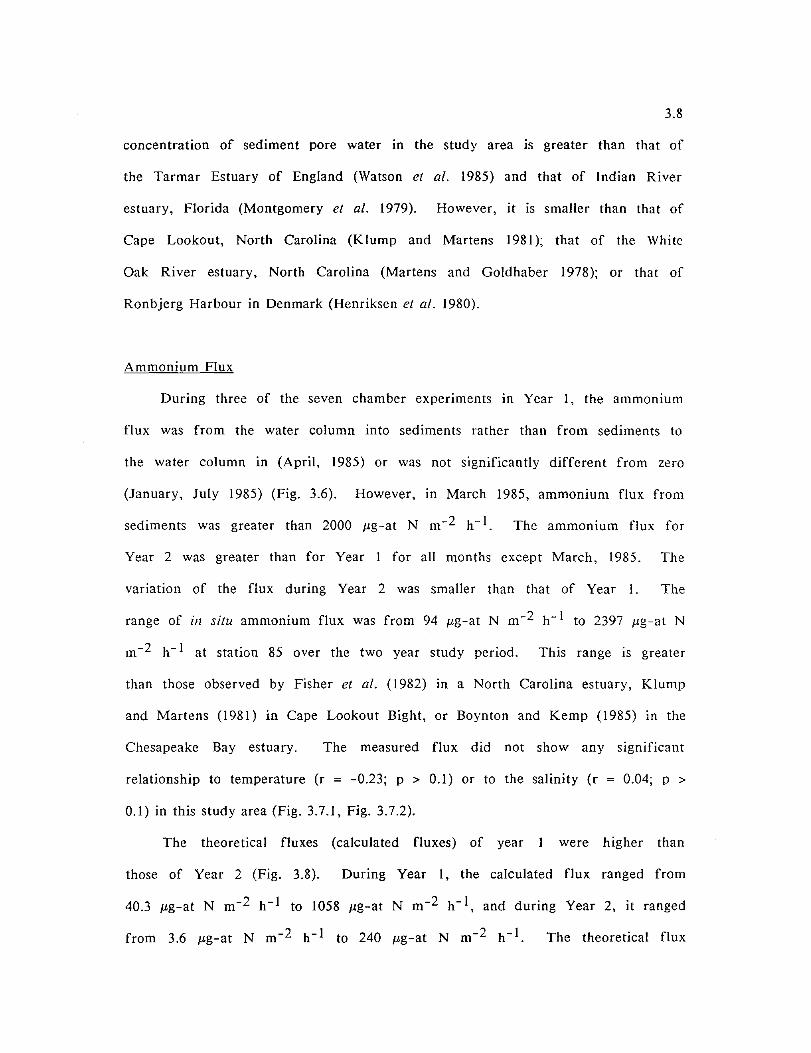
3.8

concentration of sediment pore water in the study area is greater than that of

the Tarmar Estuary of England (Watson et al. 1985) and that of Indian River

estuary, Florida (Montgomery et at. 1979). However, it is smaller than that of

Cape Lookout, North Carolina (Klump and Martens 1981); that of the White

Oak River estuary, North Carolina (Martens and Goldhaber 1978); or that of

Ronbjerg Harbour in Denmark (Henriksen et at. 1980).

Ammonium Flux

During three of the seven chamber experiments in Year I, the ammonium

flux was from the water column into sediments rather than from sediments to

the water column in (April, 1985) or was not significantly different from zero

(January, July 1985) (Fig. 3.6). However, in March 1985, ammonium flux from

sediments was greater than 2000 Ilg-at N m-2 h- I . The ammonium flux for

Year 2 was greater than for Year for all months except March, 1985. The

variation of the flux during Year 2 was smaller than that of Year I. The

range of ill situ ammonium flux was from 94 Ilg-at N m-2 h- I to 2397 Ilg-at N

m- 2 h- I at station 85 over the two year study period. This range is greater

than those observed by Fisher et at. (1982) In a North Carolina estuary, Klump

and Martens (1981) in Cape Lookout Bight, or Boynton and Kemp (1985) in the

Chesapeake Bay estuary. The measured flux did not show any significant

relationship to temperature (r = -0.23; p > 0.1) or to the salinity (r = 0.04; p >

0.1) in this study area (Fig. 3.7.1, Fig. 3.7.2).

The theoretical fluxes (calculated fluxes) of year I were higher than

those of Year 2 (Fig. 3.8). During Year I, the calculated flux ranged from

40.3 Ilg-at N m- 2 h- I to 1058 Ilg-at N m-2 h-I, and during Year 2, it ranged

from 3.6 Ilg-at N m-2 h- I to 240 Ilg-at N m- 2 h-I. The theoretical flux

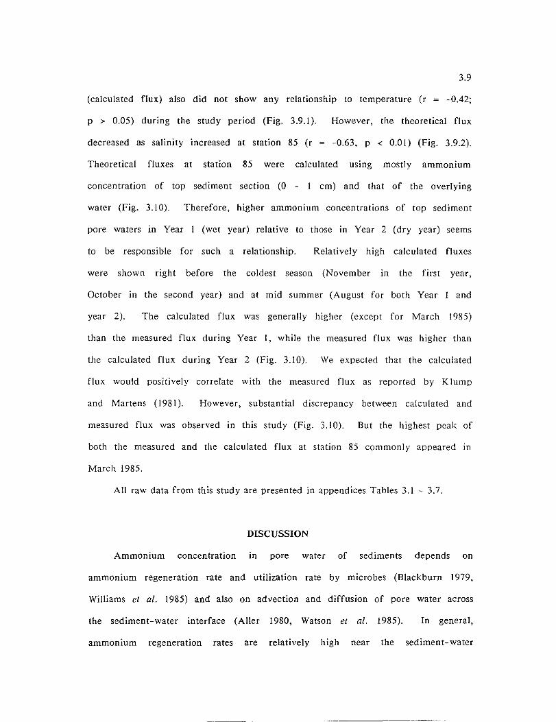
3.9

(calculated flux) also did not show any relationship to temperature (r = -0.42;

p > 0.05) during the study period (Fig. 3.9.1). However, the theoretical flux

decreased as salinity increased at station 85 (r = -0.63, p < 0.0 I) (Fig. 3.9.2).

Theoretical fluxes at station 85 were calculated using mostly ammonium

concentration of top sediment section (0 - I cm) and that of the overlying

water (Fig. 3.10). Therefore, higher ammonium concentrations of top sediment

pore waters in Year I (wet year) relative to those in Year 2 (dry year) seems

to be responsible for such a relationship. Relatively high calculated fluxes

were shown right before the coldest season (November in the first year,

October in the second year) and at mid summer (August for both Year I and

year 2). The calculated flux was generally higher (except for March 1985)

than the measured flux during Year I, while the measured flux was higher than

the calculated flux during Year 2 (Fig. 3.10). We expected that the calculated

flux would positively correlate with the measured flux as reported by Klump

and Martens (J 981). However, substantial discrepancy between calculated and

measured flux was observed in this study (Fig. 3.10). But the highest peak of

both the measured and the calculated flux at station 85 commonly appeared in

March 1985.

All raw data from this study are presented in appendices Tables 3.1 - 3.7.

DISCUSSION

Ammonium concentration In pore water of sediments depends on

ammonium regeneration rate and utilization rate by microbes (Blackburn 1979,

Williams et al. 1985) and also on advection and diffusion of pore water across

the sediment-water interface (Aller 1980, Watson et al. 1985). In general,

ammonium regeneration rates are relatively high near the sediment-water

3.10

interface and decrease with depth (Blackburn 1979, Aller and Yingst 1980,

Nixon and Pilson 1983), while ammonium concentration in sediment pore water

is relatively lower at the interface and increases with depth (Klump and

Martens 1981). Ammonium in pore water closer to the interface is more

readily utilized by benthic algae or nitrifying bacteria, and is more easily

transported into the water column. Therefore, higher turnover rates of

ammonium are probably responsible for relatively lower concentration in upper

sediment pore water compared to deeper sediments in typical estuarine

environments.

It is rarely reported that ammonium concentration in pore water of the

upper 1 cm of sediments is higher than that of deeper sediment. However

such a profile predominated during Year I (Figs. 3.5.1, 3.5.2.1, 3.5.3.1, 3.5.4.1,

3.5.5.1, 3.5.6.1, 3.5.7.1). A similar profile was reported from the tributary area

of Chesapeake Bay (Boynton and Kemp 1985). In general, during Year 2,

ammonium concentrations were either uniform through the depth of sediments

or increased with depth.

It is possible that the difference in freshwater inflow between Year 1 and

Year 2 may be responsible for the difference in ammonium concentrations of

pore waters and their profiles between Year I and 2. Primary productivity

measurements for Year are not available for comparison with Year 2.

However, freshwater inflow and inorganic nutrient concentrations were much

higher during Year than during Year 2 (Chapter 2 of this report).

Chlorophyll ~ concentration also appeared to be higher during Year than

during Year 2 (Chapter 2 of this report). Therefore, primary production of

Year I might have been higher than that of Year 2. Higher percent saturation

of dissolved oxygen during Year I supports higher photosynthetic activity in

· 3.11

Year I because higher dissolved oxygen is usually observed 10 seawater where

photosynthetic activity is more active (Sharp et al. 1982). Higher primary

production in the water column due to greater freshwater inflow may have

increased the deposition of organic matter and eventually enhanced ammonium

regeneration in upper surface sediments.

Freshwater inflow with its terrestrial organic matter may directly increase

organic deposition. In general, terrestrial organic matter contains a high

proportion of humic substances (Beck and Reuter 1974) which are refractory to

bacterial metabolism. However, it cannot be ruled out that an increase in

deposition of terrestrial organic matter may have been responsible for higher

ammonium concentrations in pore water III the upper sediments during Year I.

Even though we don't know either the pool size of total nitrogen in

surface sediments or main processes related to ammonium remineralization, we

can state that the ammonium pool in surface sediments was larger with greater

freshwater inflow in the Lavaca Bay estuary.

Ammonium flux is usually determined by III situ measurement using

benthic chambers or by using the profile of ammonium concentrations in

sediment pore waters to calculate a flux. Each of these two methods has

intrinsic limitations and assumptions. When a benthic chamber is used for

measurement, the following problems may cause erroneous results: (I)

ammonium concentration in the chamber water may change due to disturbance

of sediments; (2) non-chamber water may enter during sampling of chamber

water; (3) significant amounts of ammonium may be utilized or produced inside

the chamber; and (4) measurements in a closed system may not represent the

natural system. Calculation of the theoretical flux is based on the following

assumptions: (I) diffusion of ammonium is the main factor controlling mobility

3.12

of ammonium 1ll sediment pore waters; (2) the ammonium concentration profile

in the pore water of upper sediments is in steady state; and (3) there are no

physical, chemical or biological barriers between sediments and the sediment­

water interface which may influence diffusivity of ammonium. However, these

assumptions are not always met. For example, ammonium flux is sometimes

enhanced by bioturbation (Aller 1980; Henrikson et al. 1980; Calender and

Hammond, 1982; Lyons et al., 1982), and benthic microalgae (Henriksen et al.,

1980; Williams et al. 1985) and other microorganisms in the upper sediments

may utilize ammonium substantially prior to diffusion into the overlying water.

Flux of inorganic nutrients measured ill situ generally yields higher values

than calculated flux due to bioturbation 1ll surface sediments. For example,

Lyons et al. (1982) reported that the measured flux was 3-6 times higher than

the calculated flux at Potomac River Estuary in Chesapeake Bay, and Callender

and Hammond (1982) reported than the measured flux was 1-10 times higher

than the calculated flux in Great Bay Estuary in New Hampshire. At station

85 in the Lavaca Bay estuary, the measured flux of ammonium was 2-200 times

higher than the calculated flux during Year 2. In contrast, the calculated flux

was generally higher than the measured flux during Year 1. The sharp

ammonium gradient probably existed within a very shallow depth of sediments

during Year 1. However, ammonium concentration of the top sediment (0-1

cm) pore water and that of the overlying water were used for calculation of

the theoretical flux because ammonium concentration of the top sediment (0-1

cm) pore water was higher than that of the adjacent deeper sediments through

the year. Calculated fluxes of Year I are probably overestimated because the

ammonium concentration at the sediment-water interface is presumably much

higher than that of the overlying water. Therefore, ammonium flux measured

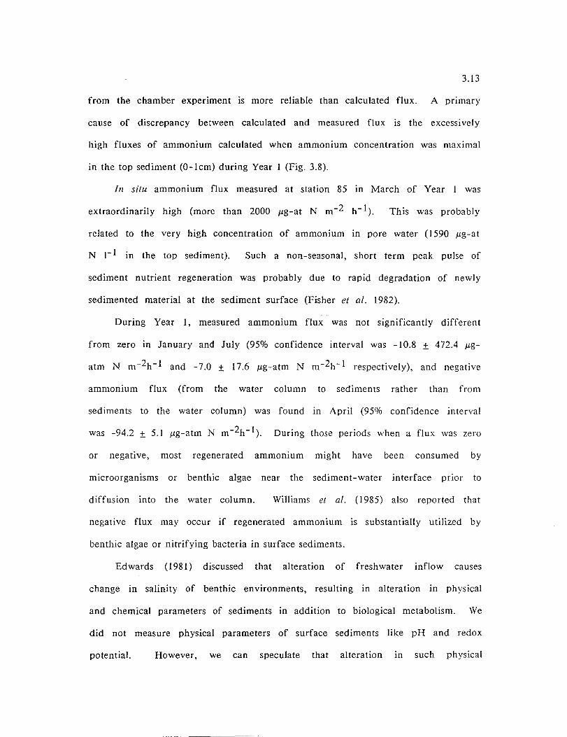
3.13

from the chamber experiment is more reliable than calculated flux. A primary

cause of discrepancy between calculated and measured flux is the excessively

high fluxes of ammonium calculated when ammonium concentration was maximal

in the top sediment (O-Icm) during Year I (Fig. 3.8).

III situ ammonium flux measured at station 85 in March of Year I was

extraordinarily high (more than 2000 J.Lg-at N m-2 h- I ). This was probably

related to the very high concentration of ammonium in pore water (I590 fLg-at

N I-I in the top sediment). Such a non-seasonal, short term peak pulse of

sediment nutrient regeneration was probably due to rapid degradation of newly

sedimented material at the sediment surface (Fisher et al. 1982).

During Year I, measured ammonium flux was not significantly different

from zero in January and July (95% confidence interval was -10.8 ± 472.4 fLg­

atm N m- 2h- 1 and -7.0 ± 17.6 fLg-atm N m- 2h- 1 respectively), and negative

ammonium flux (from the water column to sediments rather than from

sediments to the water column) was found in April (95% confidence interval

was -94.2 ± 5.1 fLg-atm N m-2h- I ). During those periods when a flux was zero

or negative, most regenerated ammonium might have been consumed by

microorganisms or benthic algae near the sediment-water interface prior to

diffusion into the water column. Williams et al. (I985) also reported that

negative flux may occur if regenerated ammonium is substantially utilized by

benthic algae or nitrifying bacteria in surface sediments.

Edwards (1981) discussed that alteration of freshwater inflow causes

change in salinity of benthic environments, resulting in alteration in physical

and chemical parameters of sediments in addition to biological metabolism. We

did not measure physical parameters of surface sediments like pH and redox

potential. However, we can speculate that alteration In such physical

3.14

parameters may be the other possible explanation for the difference in

ammonium flux between Year I and Year 2 because pH and redox potential are

important factors to mobility of ammonium (Graetz et al., 1973).

Fisher et al. (1982) reported that there was no significant relationship

between oxygen consumption rate and ill situ ammonium flux in North Carolina

estuaries. We also did not observe a strong relationship between those two

parameters In the study area. Klump and Martens (1981) observed that

ammonIUm release from sediment was strongly dependent on temperature in the

Cape Lookout Bight. In our study area, no significant relationship was

observed between temperature and in situ ammonium flux. Other processes or

parameters probably played more important roles in releasing ammonium from

sediments in our study area.

The demand for regenerated nitrogen in the water column was not

directly assessed in this study. However, simple calculations can be made to

obtain rough estimates for comparison with benthic flux measurements.

For example, one can multiply primary production (mg C·m-2·d- l ; Davis,

1986) by a conversion factor relating nitrogen uptake to carbon assimilation.

The Redfield ratio of phytoplankton (by weight 6.0 mg C·mg N-I; Redfield

et al. 1963) is commonly used for this purpose. Two examples are presented:

Month: April 1986

Primary Production: 1111 mg C·m-2 d- I

Demand for N: 1111 mg C·m -16.0 mg C·mg N- I

185.2 mg N·m-2 ·d- 1

13.2 mg-at N·m- 2·d- 1

Month: June 1986

Primary Production: 1819 mg C·m-2·d- 1

Demand for N: 1819 mg C-m-2-d- 1 6_0 mg C-mg N- I

= 303_2 mg N-m-2-d- 1

= 21.6 mg-at N-m- 2-d- 1

These daily rates could be divided by 24 to get very rough estimates of

the demand for nitrogen in units comparable to the benthic flux measurements:

3_15

April calculated demand = 550 J-Ig-at N-m-2-h- l , June demand = 900 J-Ig-at N-m-

2_h -l_ There are many problems associated with this method of estimation: the

Redfield ratio may not represent the chemical composition of the

phytoplankton (C/N might be higher, thus nitrogen demand would be

overestimated, perhaps by up to two times); bacterial demand for ammonium is

not assessed (Wheeler and Kirchman 1986) leading to a potentially sizeable

underestimation of the demand for nitrogen; nocturnal respiration of the

phytoplankton is not considered and thus the true ratio of carbon taken up

during the day to nitrogen assimilated over 24 h is underestimated and the

demand for nitrogen is overestimated, maybe by as much as 1_5 - 2 times_

There is also a problem associated with interpretation of 14C incorporation_

Does the method measure gross or net production? Without getting involved in

further discussion we can state that demand for regenerated nitrogen in the

water column is on the same order of magnitude as the measured benthic flux

(442 J-Ig-at N-m- 2-h- 1 in April, 682 /Lg-at N-m-2-h- 1 in June) and that

quantitative relationships must be determined with more involved techniques

including studies with nitrogen and carbon tracers_

CONCLUSION

The ammonium pool in surface sediments, particularly the upper few cm,

was generally higher during Year I (wet year) than during Year 2 (dry year) in

3.16

the study area. The profiles of ammonium concentrations In sediment pore

waters for the wet year were different from those for the dry year. During

the wet year, ammonium concentrations in the upper few cm of sediment pore

waters were generally higher than in deeper sediments. In contrast, during

the dry year, ammonium concentrations in the upper few cm were generally

lower than in the deeper sediments. Calculated ammonium fluxes were greater

than ill situ measured fluxes in the wet year, whereas calculated fluxes were

smaller than the measured fluxes in the dry year. Discrepancy between

calculated and measured ammonium flux may be due to overestimation of

calculated flux when ammonium concentration was maximal in top sediment (0-1

cm) during the wet year. Therefore, the measured flux represents more

reliable estimate of ammonia flux. Neither the calculated flux nor the

measured flux was correlated with temperature. Though measured ammonium

flux did not show a significant relationship with salinity, calculated flux

decreased as salinity increased. Benthic respiration rate did not show a

significant relationship with temperature or salinity during the study period.

3.17

REFERENCES

Aller, R.C. 1980. Diagenetic processes near the sediment-water interface of

Long Island Sound. I. Decomposition and nutrient element geochemistry.

Advances in Geophysics 22:237-350.

Aller, R.C. and J.Y. Yingst. 1980. Relationships between microbial distributions

and the anaerobic decomposition of organic matter in surface sediments of

Long Island Sound, U.S.A. Mar. BioI. 56:29-42.

Barlow, J.P., c.J. Lorenzen and R.T. Myren. 1963. Eutrophication of a tidal

estuary. Limnol. Oceanogr. 8:251-262.

Beck, K.C. and J.H. Reuter. 1974. Organic and inorganic geochemistry of some

coastal plain rivers of the southeastern United States.

Cosmochim. Acta 38:341-364.

Geochim.

Blackburn, T.H. 1979. Method for measuring rates of NH4+ turnover in anoxic

marine sediments, using a 15N_NH4+ dilution technique. App!. Environ.

Microbiol. 37:760-765.

Boynton, W.R. and W.M. Kemp. 1985. Nutrient regeneration and oxygen

consumption by sediments along an estuarine salinity gradient. Mar. Ecol.

Prog. Ser. 23:45-55.

Callender, E. and D.E. Hammond. 1982. Nutrient exchange across the sediment-

water interface in the Potomac River Estuary. Estuarine, Coastal and

Shelf Science 15:395-413.

Dale, T. 1978. Total, chemical and biological oxygen consumption of the

sediment in Lindaspollene, Western Norway. Mar. BioI. 49:333-341.

Davis, R.F. 1986. Measurement of primary production in turbid water. M.A.

Thesis. University of Texas.

3.18

Edwards, R.E. 1980. The influence of salinity transition on benthic nutrient

regeneration in estuaries. Proceedings of the National Symposium on

Freshwater Inflow to Estuaries.

Williams. pp. 2- I 6.

Vo!. II. Ed. by R.D. Cross and D.L.

Fisher, T.R., P.R. Carlson and R.T. Barber. 1982.

regeneration in three North Carolina estuaries.

Shelf Science 14: 101 -116.

Sediment nutrient

Estuarine, Coastal and

Flint, R.W. and R.D. Kalke. 1985. Benthos structure and function in a South

Texas estuary. Contributions in Marine Science 28:33-53.

Graetz, D.A., D.R. Keeney and R.B. Aspiras. 1973. Eh status of lake sediment­

water systems in relation to nitrogen transformations. . Limno!. Oceanogr.

18:908-9 I 7.

Hargrave, B.T. 1969. Similarity of oxygen uptake by benthic communities.

Limno!. Oceanogr. 14:801-805.

Henriksen, K., J.I. Hansen and T.H. Blackburn. 1980. The influence of benthic

infauna on exchange rates of inorganic nitrogen between sediment and

water. Ophelia, Supp!. 1:249-256.

Klump, J.V. and C.S. Martens. 1981. Biogeochemical cycling in an organic rich

coastal marine basin - II. Nutrient sediment-water exchange processes.

Geochim. Cosmochim. Acta 45:101-121.

Lyons, W.B., T.e. Loder and S.M. Murray. 1982. Nutrient pore water chemistry,

Great Bay, New Hampshire: benthic fluxes. Estuaries 5:230-233.

MacIsaac, J.J. and R.C. Dugdale. 1972. Interactions of light and inorganic

nitrogen in controlling nitrogen uptake in the sea. Deep-Sea Res. 19:209-

232.

3.19

Martens, C.S. and M.B. Goldhaber. 1978. Early diagenesis in transitional

sedimentary environments of the White Oak River Estuary, North

Carolina. Limnol. Oceanogr. 23:428-441.

Montgomery, J.R., C.F. Zimmermann and M.T. Price. 1979. The collection,

analysis and variation of nutrients in estuarine pore water. Estuarine and

Coastal Mar. Sci. 9:203-214.

Nixon, S.W. and M.E.Q. Pilson. 1983. Nitrogen in estuarine and coastal marine

ecosystems. In: Nitrogen in the Marine Environment. Ed. by E.J.

Carpenter and D.G. Capone. Academic Press, New York. pp. 565-648.

Redfield, A.C., B.H. Ketchum and F.A. Richards. 1963. The influence of

organisms on the composition of seawater. In: The Sea, Volume 2, Ed. by

M.N. Hill. Interscience, New York. pp.26-77.

Shultz, D.J. and I.A. Calder. 1976. Organic carbon 13C/2C variations m

estuarine sediments. Geochim. Cosmochim. Acta 40:381-385.

Seki, H., I. Skelding and T.R. Parsons. 1968. Observations on the

decomposition of a marine sediment. Limnol. Oceanogr. 13:440-447.

Sharp, J .H. 1982. The chemistry of the Delaware estuary. General

considerations. Limnol. Oceanogr. 27: I 0 15-1 028.

Solorzano, L. 1969. Determination of ammonia in natural waters by the phenol

hypochlorite method. Limnol. Oceanogr. 14:799-801.

Ullman, W.J. and R.C. Aller. 1982. Diffusion coefficients m nearshore marine

sediments. Limnol. Oceanogr. 27:552-556.

Waksman, S.A. and M. Hotchkiss. 1938. On the oxidation of organic matter in

marine sediments by bacteria. I. Mar. Res. 1:101-119.

Watson, P.G., P.E. Frickers and C.M. Goodchild. 1985. Spatial and seasonal

3.20

variations III the chemistry of sediment interstitial waters in the Tamar

Estuary. Estuarine, Coastal and Shelf Science 21: 105-119.

Wheeler, P.A. and D.L. Kirchman. 1986. Utilization of inorganic and organic

nitrogen by bacteria in marine systems. Limnol. Oceanogr. 31:998-1009.

Williams, S.L., S.M. Yarish and LP. Gill. 1985. Ammonium distributions,

production, and efflux from backreef sediments, St. Croix, U.S. Virgin

Islands. Mar. Ecol. Prog. Ser. 24:57 -64.

"'" -.... Q\

E '-' 0 0

"'" -.... Q\

E ...., 0 0

Figure 3.1. Stn""6S Bottom Woter Dissolved Oxygen (Station 85) Data in Appendix 3.1

15 ,-------------------------------------------------------------,

I ffi'l Yrl (1984-1985) I

10

'5

(11---.-

,JUri

Sample Date

15 ,------------------------------------------------------------,

I I

rnJ Yr2 (19:35-19;::6) I

to

5

o Oct Nov Dec "Jan Feb .Jun .Jul AlJg

Sample Date

3.21

~

lI"1 CO

10: 0 ..... ... <1l ...

U)

C I"!~ ~

c: =-> >:: 0

'C Cj

> N

C '" CI-;

:',1';: X ..... C; "0

10: (j)

'- p.. 0 p..

.,; C

" C ..... -' '" ~ '-' L rj

~ Q

~

~

10 tr)

..... .:: w u L-a;; u..

N

'" <l)

H ;:l on ..... ~

,=, if)

L L i1] .." ;:to .1.

~~~~B_~~'7$f i ~ I

Ct,

=' <C

~

-:.

c

::r. '0:;

~

c.. .;:

->:1

-

~~

3.22

..:: -;-"

0 ~

~

"" ~ I.

" 0-

N • e I.

" 0-

N Q

~

IE '-'

" ... " QC

I: 0

',," ... " I. ' .. 0-\1\

" QC

1000

800 j 600

400

200

o

Figure 3.3. Benthic chamber respiration rate. (station 85) (Data in Appendix 3.3).

• Ch 1 Electrode ~ Chl 'rvinklE-r rn Ch2 Winkler -<)- A 'I"

Nov'84 J"n'85 r'hr'85 Apr'85 r1<lIJ '85 Jun'85 Ju1'85 l\ug'85 Oct'85 D~c'85 F~b'86 Apr'86 Jun'86 Aug'86

S~mpl4! D;!h

w N W

,... ..: ~ .. a. N • E ~ .. a. N Q CI' ! .... .. .. .. IIIf:

8 ... .. .. ~ ... lao .. ..

IIIf:

Figure 3.4. I. Relationship of Benthic Chamber Respiration Rate To Temperature at Station 85 ( 1984-1986)

500.---------------------------------------------, y = 237.6 - 1.67x R = -0. t 5

EI 400 c

300 ~ EI

EI

fl r EI EI

200r---------------------~;-o-~--~------______ ~ EI

EI

EI EI

cP f I EI 100~----~-------L-------L------~------~--~~

o 10 20 30

Tempanlura (·e)

Figure 3.4.2. RelationshIp of Benthic Chamber Respiration Rate To 561inity at Station 85 ( 198 ... -1986)

500.---------------------------------------------, y = 137.0 + 5.65x R = -0.45

400 EI

300

200

EI

l00~------~-----W~------~------~------------~

o 10 20 30

S.linily (,pi)

3.24

3.25

ngure- 3.5. L PrC'fi les .of anmonium concentrations in sediment pore waters at station 45. (Data in Appendix 3.4)

1000

1500

1200

900

600

300

o

IliI Con--I

G3 Cor .. 1112

0-1 1-2 2-:I 3-4 4-5 5-<i 6-7 7-S 6-9 9-10

"",'h(an)

Sln "'"45: 12/4/05

0-1 1-2 2-3 3-'4 '4-:5 ::5-6 6-7 1-6 6-' 'J-1O

Stn -45: 2/5/66

~,-----------------------------------~

200

100

0-1 '-2 2-3 1-4 4-5 !i-E> (,-7 1-8 8-' '-10

Stn '45: 4/9/66

~r-------------------------------'

200

0-1 1-2 2-3 3-4 "-5 5-6 6-1 7-8 6-' '-fO

Stn • 45: 6/4/66

~Qr---------------------------------------'

0- I I .. ;> 2 .. .5 3. - '" .( .. s s .. (, (, .. ., ,. .. B B .. 9 9 .. 10

Stn • 45: 6/6/66

~r-------------------------------~

200

100

0-1 1-2 2-3 3-4 4-5 5-6 6-7 1-8 8·' 9-10

3.26 Figure 3.5.2.1. Profiles of ammonium concentrations in sediment pore waters

at station 603 in Year 1 (Data in Appendix 3.4)

(Hlf..1I(J1Q-.&lm NIl)

(NIH I (jlQ- ... tm NIl)

'N"41 Wq-.(m H/1)

1800

1500

1200

"00

WO

'00

0-1 1-2 2-3 ::,\-4 4-5 5-6 6-7 7-G G-9 9-10

de-pth (un)

113 Corf' -,

iii Corf' c 2

0_=-'='"

1800

1500

1200

'JOO

600

300

o

0-' 1-2 2-3 3-4 4-5 5-6 6-7 7-8 e-9 9-10

dt-pth (em)

0-1 t-2 2-3 !-4 4(-5 5-6 6-7 1-9 &-9 9-\0

d~th(cm)

.. Con- -.

m Corf' -2

... " .... ('(".&~

0-1 1-2 2-Z 3-4 4-5 5-6 £,-1 1-9 9-9 9-10

d<pth (em)

(NtH I CalQ-... lm HI!)

1200

'JOO

'JOO

7SO

(NIH I Qtq- ... tm 450 NIl)

1800

1500

1200

900

1800

1500

1200

110141 WQ-.(m 'JOO

HII)

fnJ"

300

o

iii Cor. "I

m Corf' c2

.. - Av~~

0-' 1-2 2-3 !--4 4-5 S-G 6-7 7-8 9-9 9-10

do..'Pth(cm)

Stn-ros: 6/'5/85

IICoa-'

[§ Corf' c 2

0-1 1-2 2-3 !-4 4-5 S-6 £-7 7-B 8-9 9-10 dt-pth (Cf(,)

GI Cort- -1

m wf'-2

-+- AVK;'~

0-1 1-2 2-3 !--4 4-5 5-£ 6.-7 7-B 6-9 ':1-10

dEt,!h (an)

• Corf' -,

mJ Corf' -2

... AI(K'~

0-1 1-2 2-3 !-4 "-5 S-o 4>.-7 1-8: G-9 9-10

&!>th(an)

· · ~

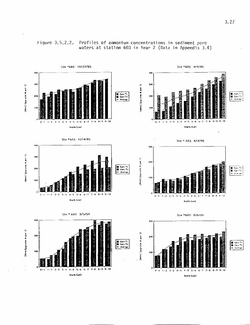
l

" · ~ ! ~ ~ ~ x ~

3.27

Figure 3.5.2.2. Profiles of anrnonium concentrations waters at station 603 in Year 2

in sedi ment pore (Data in Appendix 3.4)

'00 ,----------------------,

Stn -603: 12'4/65

'OOr-----------------------------------------,

{'I-I 1-2 2-;3: 3--4 -4-'S SOb 6-7 7-8 8-'99-10

Sln .. 603: 2/5106

wo

200

0-1 1-2 2-3 3-04 .-s 5-6 '-7 7-8 8-'51 9-10

" ~ « ! ~ !;

I

• x <

. ~

lOO

200

100

0-1 1-2 2-~ ~-.04 "'-'S 'S-6 0-1 1-0 o-~ q-IO

Stn - 60J" 6/4/06

Stn -603: 0/6/06

!ill ,-------------------~

(1-1 1-2 2-3 3-4 4-5 S-(' 6-7 7-8 eo' '-10

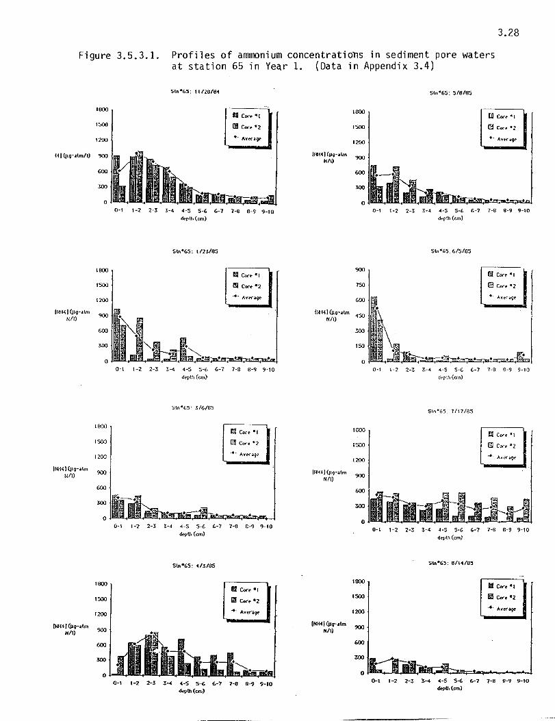
3.28

Figure 3.5.3.1. Profiles of ammonium concentrations in sediment pore waters at station 65 in Yeqr 1. ( Data in Appendix 3.4)

S1n-6:J: t 1120/01 $(0"&5: 5/0/65

100J

lUI Cor~ tI' 1000 IlB Coo tI,

1500 Il! Ur~·2 1500 C9 COI"f ·1

1200 +. A't't("~9f' 1200

+. AVH"';'¥

HI (jtq-.I.tm/l) 'lOO If.1H041 (Vroltm 'lOO NIl)

600 600 Ilb-.,<-. :lOO :lOO

0 0 +

0-1 1-2 2-' '-4 4-5 5-6 6-1 1-6 8-, 9-10 0-' 1-2 2-' !-4 4-5 5-. 6-1 7-8 8-9 9-10

d<1'tt, (em) <kpth (em)

Stn·65: l/n/65 $tntl65: 615/65

100J II!I Cu"f' «, <;00 m: Wt .,

'500 t'J Corot ·2 150 ~ Co.-l'·2

1200 .,.- AVK.l9E'

600 .+. A.vi;r~

IHIHI<llq-.I.tm 'lOO

I, ... I WQ-.tm 450 NIl) HII)

600 :lOO

:lOO '50

0 0 (}-I 1-2 2-3 ~-4 4-5 5-6 6-1 1-8 8-9 9-10 0-1 1-2 2-Z !.-4 4-5 5-. 6-1 7-8 8-9 9-10

depth (em) d~th (em)

Stn tlE.S: '5/6/85 51n·65_ 7/17/85

I BOO M Corf' ., 1000

£3 Con ·1 1500 11!1 eor. tl 2 1500 Gl COCt ·2

1200 .+. Avtr .. qi' .+. A'(ff'~

1200

ItaH)WQ-.tm 900 IHI-HJ Wq-.I.tm HII)

lUI) 900

600 600

:lOO :lOO

0 0

0-1 1-2 2-3 '-4 4-5 5-6 6-7 1-8 B-' 9-10

de-pU. (em) 0-1 '-2 2-3 3-4 4-5 5-6 6-1 7-8 s-. 9-10

dt'pth (em)

Stn-6oS: 4,/3/85 Stn-6:l: B/'"/~

1800 1800 II tort' ., II tort .,

1500 l! Core- tl 2 1500 m Cor. -2

1200 -+. Ayer~ 1200 ... A,(ff~

II.H)WQ-.tm (t<H4)W.,.-.tm 900

NIl) 900 Nil)

600 600

:lOO 300

0 0

0-' 1-2 2-3 ,-< 4-5 5-'; £-7 7-8 8-9 9-10 0-1 1-2 2-3 3-< 4-5 5-6 6-7 7-B 8-9 9-10

<l<,>th ("',J <l<,>fr,(anl

Figure 3.5.3.2. Profiles of ammonium concentrations in sediment pore waters at station 65 in Year 2. (Data in Appendix 3.4).

Stn 665: IO/2~/05 Sfn "'65: 4/9/06

4(jt}

" soo ~

c

~ ~ ~ . E

0-1 '-22-33-4 4-S ::>-6 6-1 l-S 8-' '-10 0-' 1-2 2-J 3-4 4-=- 5-6 6-7 7-8 8-' '-10

Stn -65· 12/4/05 Sln "65: 6/4/66

.OOr-----------------------------------------, NO,-------------------------------,

00

0-1 1-2 2-:!> l-~ 4-5 5-6 6-7 7-S S-'9 '-10

~u,(c .. )

Sfn "65 2/5/06 Sln '(is: 0/6/06

>W,-------------------------------,

0-1 1-2 2-3 3-4 4-S S-6 &-1 1-8 8-' '-10 0-1 1-2 2-5 3-4 4-5 5-6 6-7 7-8 8-' '-10

3.29

Figure 3.5.4.1.

1000

1500

1200

H. (jt9-.1m/1) 'JOO

600

300

0 0-1 1-2 2-3

1000

1500

1200

U.14)(VO-·1m NIl)

600

300

0 0-1 '-2 2-3

1800

.500

'200

(NIH I (VO-.1m 900

lUI)

600

300

a 0-1 1-2 2-3

lSOO

1500

1200

( .. «I (jt<r.1m 'JOO HIO

600

300

0 0-1 1-2 2-3

3.30

Profiles of ammonium concentrations in sediment pore waters at station 613 in Year 1. (Data i·n Appendix 3.4).

Stn·613: Il/zu/04 Stn·61~: ~/B/ttl

1000 CII Corf' -I

I soc ~ Cor~ -2

1200 ..... AVffj¥

(NIH J Cttq-.ltm 'JOO

"It)

600

300

0

3-4 4-5 5-6 6-7 7-. 8-9 9-10 0-1 1-2 2-:!; 3-< '-5 5-6 6-7 7-8 .-9 "",to (em) &opt"to (em)

Stn-61 ~: 11Z~/6~ Stn·613:6n/s:l

9-10

til Cort' -r--Ell Core--'

900 E! wt'-2

I!1lI Coc.·2 7SO

.... "'Vff.l¥ 600

INH4 I (~9-.tm "It) 'so

300

ISO

0 3-' 4-5 5-6 6-7 7-8 e-9 9-10 0-' '-2 2-~ 3:-4 <-5 5-{; 6-7 7-8 8-9 9-10

d ... ptt. (em) d.i-plh (ern)

Sln-G!!:: 3/6/B~ Slo C 6t5- 7/17/65

M Cur ... , .eoo 1m W"t"-I

(3 CCN'"t' ·2 '500 a Cor. -2

.•• Avt"riqt' .. - AV"("~9'"

'200

1!.,tH4' (I1Q-oltm NIl)

'JOO

600

300

3-< '-5 5-{, 6-7 7-8 .-9 9-10 0

depth (em) 0-' 1-2 2-3 3-4 '-5 5-{; 6-7 7-. .-9 9-10

o<"pth (em)

5tn-615: 1/3/B:.'I Stn-6!:!;: 8/11/85

III CorP at 1000

E Coc-. &2 II Cor"t &.

1500 19 1:«. &2 ..... AV«~

1200 -+-A!(f:t'q

(/Ii.(jt,-.1m 'JOO HIO

600

300

3-< '-5 5-{; 6-7 7-9 8-9 9-10 0

"",Ih(em) . 0-' 1-2 2-' 3-< '-5 5-<; 6-7 7-S 8-9 9-10

"",U.(cm)

. !

• !

3.31

Figure 3.5.4.2. Profiles of ammonium concentrations in sediment pore waters at station 613 in Year 2. (Data in Appendix 3.4).

~;(n ·6 I J 10/2J/05

Stn '611 1214/85

wo,---------------------------------,

0-1 \-2 2-3 3-" '4-5 5-6 '-7 7-8 8-99-10

5tn "6 I 3: 2/5/06

~r-------------------------------__,

0-1 (-2 2-3 3-. <I-S s-, '-7 7-8 8-' ,·10

IN1oU. (~)

5tn ·61.1: 4/9/66

~~r-----------------------------------,

0-\ 1-2 2-3 1-'4 .-~ ~-6 6-7 7-8 8-' ,-to

Sln '(I t 3: 0/6/06

(I-I 1-2 2-3 3-. 04-5 5-6 6--1 7-8 8·,9-1('

3.32

Figure 3.5.5.1. Profil es of anmoni urn concentrati ons in sedi rnent pore waters at station 623 in Year 1. (Data in Appendix 3.4).

1 COO

1500

1200

HI tttq-.atm/l) 900

600

wo

o

1800

1500

1200

900

1000

1500

1200

S(n -62?;: 11/ZE/C'1

0-1 1-2 2-3 3-4 4-5 S-6 6-7 7-8 8-9 9-10

d<-?th (an)

0-1 1-2 2-3 3-4 4-5 S-~ 6-7 7-S 8-9 9-10

d<,ptl'l (em)

0-1 1-2 2-3 !-4 <4-5 S-6 6-1 7-8 8-9 9-10 d<-?th (an)

(r.a-l4! UrQ-..Jtm Nil)

1000

1500

1200

600

wo

o

1800

1500

1200

900

600

WO

0

1800

1500

1200

0-1 1-2 2-3 3-4 4-5 5-6 6-7 7-8 8-9 9-10 &!-rU, (em)

Stn IC 623: 7/17/~

tI Cor~ -I

@ Cor. -2

.... Aytr.l¥

Ik~,\.'" (rod

0-1 1-2 2-3 3-4 «-5 5-6 6-7 7-8 8-9 9-10

""'",(an)

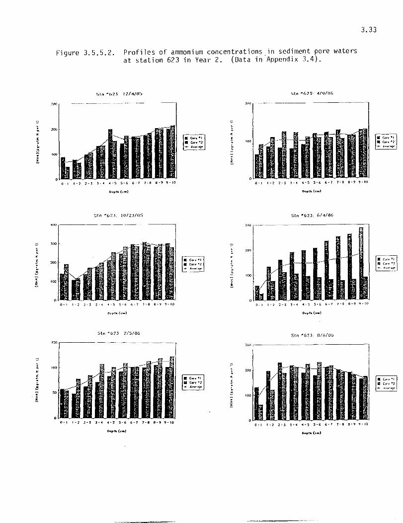
" L

· • , · ~ -; !

3.33

Figure 3.5.5.2. Profiles of ammonium concentrations in sediment pore waters at station 623 in Year 2. (Data in-Appendix 3.4).

~;ln "liZ'} I ]/4/t1:,

.'.tlOj ---- - ----- - ----------- ---

~ln "'"67.3 10/23/U5

.00,--------------------------------------,

200

'00

Stn '"'623 2/5/06

.~.---------------------------------,

0-1 1-2 2-3 3-4 4-~ 'l-6 6-7 1-8 (1:., '-fO

• , ,

· x <

" · E

.'7

· ,

< E

,

·

Sln -623: <'I/~/IIG

0-1 1-2 2-;5: 3-4 4-5 5-6 6·7 7-8 8-' '-10

Sln '623: 6/4/86

,~.--------------------------------.

""

'00

~u.(_)

SIn '62J: 0/6186

!.(.) ,----------------------,

~(lI(C"")

3.34

Fi gure 3.5.6.1. Profiles of ammonium concentrations in sediment pore waters at station 633 in Year 1. (Data in Appendix 3.4).

1 BOO

1500

1200

900

600

(]

1800

1500

1200

900

600

0-1 1-2 2-~ 3-4 -4-5 5-6 6-7 7-B 8-9 9-10

"",th(an)

0-1 1-2 2-3 !-4 4-5 S~ 6-7 7-8 8-9 9-10 ",,,th(an)

H,", I (JJ,-.tm 1</I)

7SO

600

.,,"

1 BOO

1500

1200

900

600

300

(]

Ill! Core-'

0-1 1-2 2-!;' 3-4 4-5 S-6 6-7 7-8 8-9 9-10

&pth (em)

0-1 1-2 2-3 3-4 4-5 5-6 6-1 7-8 8-9 9-10 deopth (em)

· ·

· r E

E

E

, a · r to

3.35

Figure 3.5.6.2. Profiles of ammonium concentrations in sediment pore waters at station 633 in Year 2. (Data in Appendix 3.4).

Sln "fill: IO/23/0'...i

MOI----~---~~~~~~~~~~~~

0- I 1 _ 2' :1 -.;. 3: -.. .. - S '5 - (, b - 1 - G S - 9 ~ - 10 0-1 1-] 2-3 3-« 4-5 S-(, (.-7 J-e G-'1 9-10

5tn -633> 12/4/05 Stn • 633 : 6/4/66

~.-~~~~~~~~~~~~~~~~~,

cOO

~ 50)0 .... " E '00 . ,

;00 .. C . 200 :r 5.

100

0 0-\ 1-2 ]-! S-" "-5 5-6 6-7 7-8 8-99-10 N '" ... '" 0- " .. 0

0 N '" D~pth (em) '" 0- ",.

SIn '6JJ 215/06 Stn *(,33: O/(j/(Hi

("'r-~~~~~~~~~~~~~~~~,

" · · ! , · a · "" • E"

0-1 \-1 ]-5 3-0( ,,_S S-E- "'-1 1-S 8-99-10

• (.(0:"'" .,

i!i Corj> -2

A¥~.1'?

3.36

Figure 3.5.7.1. Profiles of ammonium concentrations in sediment pore waters at station 85 in Year 1. (Data in Appendix 3.4).

(lti<l(p.-.im fill)

(lti<l W.-.lm HI.)

)HH41 WQ-.lm HIt)

(/IH<1 W.-.lm 1(1t)

1000

ISOO

I BOO

1500

'200

900

600

WO

0

1800

'500 '200

900

600

WO

0

1 BOO

1500

1200

900

600

roo

0

Sln -o:s: 11/2818-4

0-1 1-2 2-3 3-<1 <4-'5 5-6 6-7 7-8 8-9 9-10 "",'h(",,)

Stn -8S: 1/23/85

II C«~ as ~ Core -2

0-' '-2 2-' ,-4 4-S S-<; 6-7 7-8 8-9 9-10 tkpltl (em)

Sln·~: 3/6/SG

0-, 1-2 2-' ,-' 4-5 s-<; 6-7 7-8 8-9 9-10 d<-pu.(",,)

Stn·~: 4,/3/8:)

II Cor-t -I

S Cor.-2

-+- Avet'.

0-1 1-2 2-3 ,-' 4-5 s-<; (,-7 HI. 8-9

"",U.(an)

("H') WQ-.lm H/l)

(14-14) WQ-.lm Hit)

Stn-ss: :s/8/es

7SO

"'0

° ---"' ....

900

7SO

600

"'0 300

ISO

0

1800

1500

'200 900

600

300

0

0-1 1-2 2-3 3-4 4-5 S-£ ~-7 7-8 S-9 9-10 df-plh(an)

Stn-S5:6!':i!BS

0-' 1-2 2-' 3-4 <-5 5-<; 1;-7 7-8 8-9 9-10

d.:-pU\ (em)

5to-8::5: 7/17/8:)

IS Con- -I

8 Cor(' C2

.. - Aver .. q ..

0-1 1-2 2-3 3-4 4-S S-<; 6-7 7-8 8..,.9 9-10 "",u. (om)

· • ! · · ~

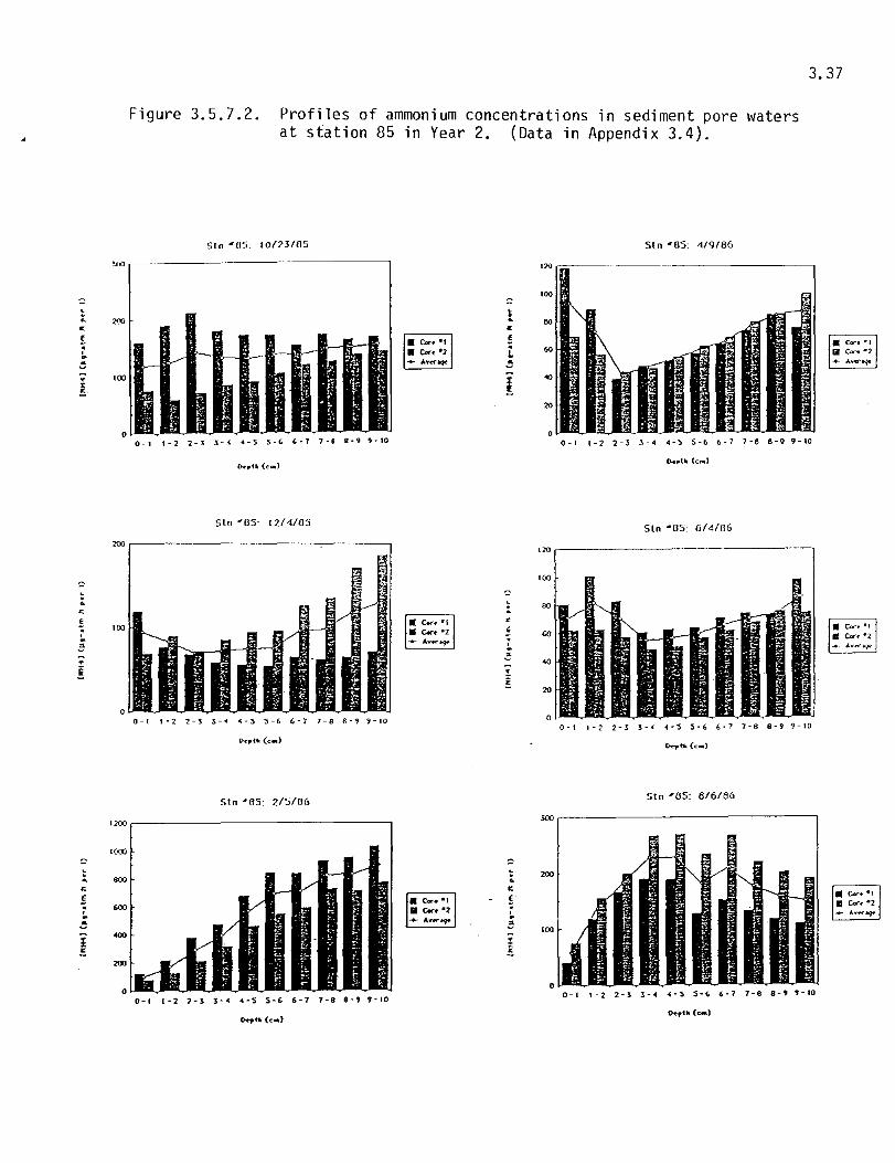
3.37

Figure 3.5.7.2. Profiles of ammonium concentrations in sediment pore waters at station 85 in Year 2. (Data in Appendix 3.4).

SIn "OJ: 10/23/05 Stn '05: 4/9/66

=.---------------------------~ I~r.o~------------------------------------_,

0-1 1-2 2-1 1-4 4-5 5-6 6-7 1-11 8-99-10 0-1 1-2 2-3 ~-4 4-5 5-6 6-1 7-6 8-99-10

Sln "OS· 12/4/05 Stn '05: 6/4106

xo,-------------------------~--------, I~.-------------------------------------,

0-1 1-2 2-3 3-4 "<5 5-6 6-7 7-8 8-' '-10 0-' 1-2 2-3 3-4 4-!i 5-6 6-7 7-8 8-' '-10

Stn '05: 2/5106 Stn '05: 6/6166

I~r-----------------------------------,

" t 200

• 1 ~ 100

• !

0-1 1-2 2-3 3-4 4-'5 5-6 6-1 7-8 8-' '-10

Ck,th (c:",,)

.... .I:

~ • Do.

N c E ~ • Do.

IE

! .. " ~ ::I. .., Ie :I ... II.

.... .I: ~

I N c E .. I IE ! .. " I ClIO .. .., Ie :I ... II.

Figure 3.7.1. Relation:.hip of Heaured AIIImonium Flux Fro. In Situ Chamber:. To Temperature at Station 85 ( 1984-1986)

~r---------------------------------------------~ y R 1041.2 - 22.57x p. -<>.23

2000 f-

[)

(]

(] (]

~

(] Ii]

o (] Ii]

0 [) (]

-1000~------~----~'~----~~----~'~----~-------J

o 10 20 30

Tempanture ("C)

Figure 3.7.2. Relationship of Measured Ammonium Flux From In Situ Chambers To Salinity at Station 85 (1984-1986)

3000.----------------------------------------------. y =517.0653 + 4.1838x R = 0.04

0

2000

[)

1000 (]

e e [)

[) [)

Ii]

Or e Ii] [) e

-1000 I --'

0 10 20 30

Salinity (ppL)

3.39

,... ,/: .. " A-

N • E .. " A-Z

e .. II I 11\ =. .... )( ~ ...

Woo

Figure 3,6,

2S00 I

1500

SOO

Ammonium flux measured from in situ chambers at station 85, (Data in Appendix3,6l,

..I I_ e"-1 m C"-2 .~. 'AVE

-500~1 --------~----~--------_r------~----~-----~----T_--~------~------~--~------_r--------~--~ Nov'e4 Jan'S5 t1ar'SS Apr'8S t1~'I'E:5 ,.lun'E:5 Jul'85 Aug'S5 Clef8S D,0'85 F'tb'S6 Apr'S6 Jun'S6 A'J9'S6

Sample Date

w w 00

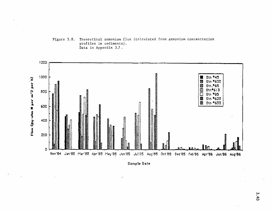
..... J:. .. " 0. (II 4 e .. " 0. z e .,. " I G'I :I.

"wi

)( :I ,. w.

Figure 3,8, Theoretical ammonium flux (calculated from ammonium concentration profiles in sediments), Da ta in Appendix 3.7 '

1200 ~I ------------------------------------------------------------------------~

1000 • Stn -45 B Stn -60!. m Stn,-65

SOO ~ Stn a613 o Stn -S5

, I!II Stn -623 m Stn -63!.

600

400

200

o I !ILl "

Noy'S4 ,lan'SS Mar'e5 Apr'S5 f1a lJ'S5 ,lIm'SS Ju 1'::: 5 AU9'S5 Dot'aS Do,o'85 r('b'SE, Apr'S6 Jun'S6 AUQ'S6 ,

SamplE.' Date

w ~ o

'" .t:. ~ • ct. ('t

• IE ~ • ct. z IE .. .. I.. :::L ...., X • -'"

,.. J: ~ • ct. ('t • IE .. • ct. z ! ..

I GO :::L """

figure 3.9.1. RelationShIp of TheOretical AalmonlulIl flux To Temperature at Station 85 (1981-1986)

~r--------------------------------------------'

0 0

y. 516.9 - 13.:?x R ~ ~.42 o

10 20 30

Temperature (-e)

Figure 3.9.2. Relationship of Theoretical Ammonium Flux To Salinity lit Stotion 85 ( 1981-1986)

600.----------------------------------------------,

o y • 476.5 - 21.9x R = -0.6:;·

600

400

200

o

10 20

Salinity (,pU

3.41

~

Figure 3.10. Comparl son or Theoret1cal Ammonium FlUx With Measured Flux at Station 85

3000~i ----------~~~~::~::~~~--------~=========:--~ • Measured 1m Theoretical

1 2000

~ I • J " ! !

1000

o

[Numbers above bars corre!!pond to method used to calculate theoretical ammonium nux. See Appendix 3,6 for detail!!)

-10001~--~----------------~----------------~--------------~ Nov'B4 Jan'BS Mar'SS Apr'6S May'6S Jun'BS JurBS Oct'BS Oec'BS Feb'B6 Apr'S5 Jun'B6 AUQ'B5

Month

<..I . "'" N

Table 3.1. Porosity of Sedl menu 3.43

Porosity = «sample vet veiQht-sample dry velQht) lsample volume) t 1 00 Semple Volume '" (3.3)A2 * 3.14 = 34.19 em

A3

3tation .- Depth Apr'66 Jun'66 AUQ'66 station # Depth Apr'66 Jun'S6 AUQ'66 (em) % (g/emA3) AVE (em) % (g/emA3) AVE

45 0-1 56.9 71.7 69.9 66.8 603 0-1 71.5 66.5 67.5 75.2 1-2 68.7 89.9 48.S 69.0 1-2 87.4 80.1 65.9 77.8 2-3 61.8 58.0 46.2 55.3 2-3 89.9 85.9 63.~ 79.9 3-4 56.8 68.1 48.3 57.7 3-4 83.3 87.9 70.9 80.7 4-5 53.9 80.4 50.2 61.5 4-5 84.9 86.2 71.3 80.l1 5-6 41.3 85.9 46.6 57.9 5-6 78.9 89.3 61.6 76.6 6-7 48.2 73.4 43.9 55.2 6-7 77.1 84.9 78.5 80.2 7-8 44.5 78.2 37.9 53.5 7-8 86.5 87.8 68.6 81.0 8-9 45.4 70.1 41.2 52.2 6-9 86.3 91.3 72.6 63.5

9-10 34.1 62.9 46.1 47.7 9-10 87.1 82.1 64.6 77.9

65 0-1 66.2 56.0 61.9 66.0 613 0-1 61.8 65.3 60.0 69.0 1-2 61.3 44.1 54.2 53.2 1-2 77.6 82.2 77.8 79.2 2-3 41.1 36.8 55.1 44.3 2-3 80.3 80.2 85.4 82.0 3-4 37.4 38.4 57.1 44.3 3-4 74.7 69.1 93.4 79.1 4-5 66.2 38.9 49.9 51.7 4-5 75.7 65.6 81.8 74.4 5-6 61.5 35.1 58.3 51.6 5-6 73.0 64.4 77.5 71.6 6-7 60.0 31.7 51.4 47.7 6-7 70.3 72.3 79.8 74.1 7-8 64.9 39.9 45.9 50.2 7-8 71.5 68.3 80.7 73.5 8-9 47.4 54.3 43.3 48.3 8-9 75.6 64.2 76.3 72.0

9-10 60.7 43.4 45.8 50.0 9-10 69.5 90.2 78.9 79.5

85 0-1 79.4 70.9 69.4 73.2 623 0-1 81.6 68.6 81.6 77.3 1-2 60.3 68.1 71.3 66.6 1-2 69.8 80.7 61.5 70.7 2-3 64.8 67.5 71.5 67.9 2-3 58.9 69.2 64.3 64.1 3-4 61.0 73.9 54.1 63.0 3-4 60.8 58.9 60.9 60.2 4-5 62. I 73.9 60.1 65.4 4-5 59.6 55.1 58.0 57.6 5-6 89.4 68.9 70.1 76.1 5-6 58.1 61.3 59.8 59.7 6-7 64.7 62.8 55.0 60.8 6-7 60. I 59.4 55.2 58.2 7-6 62.4 61.6 72.4 72.1 7-8 69.6 61.0 60.5 63.7 6-9 75.5 61.9 51.8 63.1 8-9 55.6 57.1 50.9 54.6

9-10 74.0 77.8 63.7 71.8 9-10 56.0 54.8 59.3 56.7

633 0-1 73.0 69.9 72.7 71.9 \-2 51.9 56.8 67.3 58.7 2-3- 54.9 47.4 63.7 55.3 3-4 60.3 43.6 65.1 56.3 4-5 59.\ 45.9 60.9 55.3 5-6 59.6 38.3 75.\ 57.7 6-7 66.0 42.4 68.8 59.1 7-8 68.9 37.8 61.6 56.1 8-9 63.0 31.8 65.2 53.3

9-10 54.4 47.4 63.8 55.2

,

I t

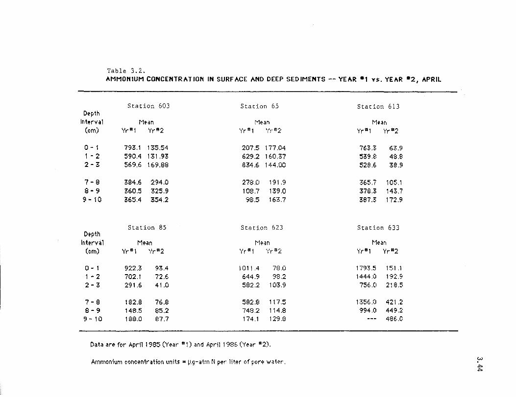
Table 3.2. AMMONIUM CONCENTRATION IN SURFACE AND DEEP SEDIMENTS -- YEAR -, YS. YEAR -2, APRIL

Station 603 Station 65 Station 613 Depth

Interval i"lean t-lean ~1earl

(om) '{I' "1 ~'r"2 'r'r "1 Vr#2 1'rlll 'r'r"2

0- 1 793.1 135.54 207.5 1 77 .04 76:::.::' 63.9 1 - 2 590.4 131.93 629.2 160.37 539.E: 48.8 2-3 569.6 169.88 834.6 144.00 52·9,6 38.9

7-8 384.6 294.0 278.0 191.9 365.7 105.1 8-9 360.5 325.9 108.7 139.0 378.3 143.7 9 - 10 365.4 354.2 98.5 163.7 387.3 172.9

Station 85 Station 623 Station 633 Depth

Int~rval M~an Mean ~1earl

(om) Yr "1 '(1'112 ','r III \),.#2 'l'r II 1 Yr"2

0- 1 922.3 93.4 1011 .4 78.0 179:::.5 151.1 1 - 2 702.1 72.€. 644.9 98.2 1444.0 192.9 2-3 291.6 41.0 582.2 103.9 75€ .. O 218.5

7-8 182.8 76.8 582.8 117.5 1356.0 421.2 8-9 148.5 85.2 748.2 114.8 994.0 449.2 9 - 10 188.0 87.7 174.1 129.8 486.0

Dah ar~ for April 1985 (Y~at' 111) and April 1986 (Y~ar lI2).

Ammonium ¢onc~ntration units = p.g-atm 1'1 per lit.~r of pore W~\"I·. w .j:> .j:>

Table 3.3. AMMONIUM CONCENTRATION IN SURF ACE AND DEEP SEDIMENTS -- YEAR -1 YS. YEAR -2, JUNE

Station 603 Station 65 Station 613 L'~ptl"t

Irlt~rva 1 f"l~an tvlo?n f"lean (ern) ','1" "I ",' r #2 y r 1:t1 ~IJr #2 Yrlll 'r'r1l2

0- 1 259.5 67.8 521.1 53.6 678.6 65.7 1 - 2 169.9 84.3 104.1 81.0 747.3 75.6 2-3 213.0 84.0 74.4 :35.5 582.2 n.E.

7 - 8 160.5 159.6 26.2 44.0 365.4 74.8 8-9 243.8 178.0 21.2 69.3 200.'? 92.5 9 - 1 (I 192.2 193.1 64.9 41.3 202.1 115.1

Station 85 Station 623 Station 633 D~pth

Int~rval Mean t-lean 1'1edr, (om) ','1" "I "1'r#2 ','r "I \'1'''2 'l'r ll l Yrll2

0-1 225.7 71.1 16.0 43.1 66.6 121 .4 1 - 2 120.7 81.9 117.2 105.4 372.0 352.7 2-3 133.4 70.2 30.1 136.5 84.::- 393.4

7 - 8 54.3 71.1 :'::';;,8 165.1 105.4 8-9 103.0 74.4 51.8 172.6 9 - 10 148.2 86.5 30.7 18';'.2 227.9

L'at .. are fe,r JIJM 1985 ('rear 111) and . .Iuno? 1986 (')"ear 112)

Ammonium I,oncentration units = p.g-at.m r-I pel" liter ,)f pore "/.at",r.

w .j:> U'I

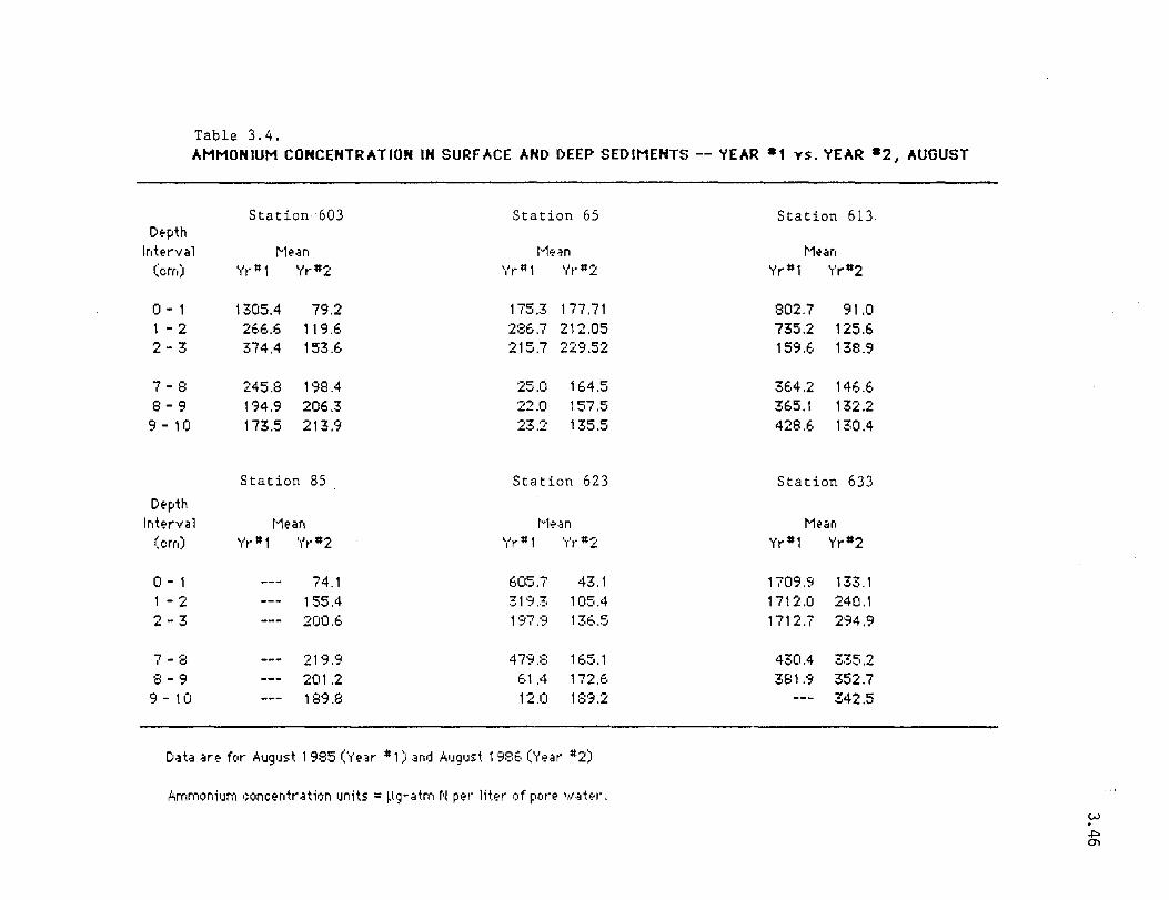
Table 3.4. AMMONIUM CONCENTRATION IN SURFACE AND DEEP SEDIMENTS -- VEAR 81 YS. VEAR 82, AUGUST

DE'pth Irlterva 1

(em)

0-1 1 - 2 2-3

7-8 8-9 9 - 10

DE'pth Irlterval

(ern)

0-1 1 - 2 2-3

7-8 8-9

9 - 10

Station 603

F"1~an

Yr 1$1 'tr "2

1305.4 79.2 2€·6.6 1 1 9.6 374.4 153.6

245.8 198.4 194.9 206.3 173.5 213.9

Station 85

r1ean ~Jr 1$1 'ir "2

74.1 155.4 200.6

219,'3 201.2 189.8

Station 65

tvl>?~n

Vrtt1 ~1)r#2

175.3 177.71 286.7 212.05 215.7 229.52

25.0 164.5 22.0 157.5 23.2 135.5

Station 623

t·'I",.;n ~IJr u 1 'y'r #2

605.7 43.1 319.3 105.4 1';<7.9 136.5

479.::: 165.1 61.4 172.6 12.0 18'3.2

D~t~ ~re for A1J9'Jst 1985 (Ye.3r # 1) and AIJgIJS1 1986 (Y",ar #2)

ArnmonilJrn ')oncentr ation units = ~\'l-~trn N P>?I- lit.l?r ,~f pore ',of·3ter.

Station 613

M~ar,

Yr#1 'r'r#2

802.7 735.2 159.6

364.2 365.1 428.6

91.0 125.6 138.9

146.6 132.2 130.4

Station 633

t'1~.;,rl

Yr"l Yr"2

1709.9133.1 1712.0240.1 1712.7 294.9

430.4 335.2 381.9 352.7

342.5

w -I'> Cl'l

3.47

Appendix 3.1 Bottom Water Dissolved Oxygen Concentration (Station 85)

Sample Bottom Date Water DO

(mg/I)

Year I

11/28/84 10.7

1/23/85 12.0

3/6/86 9.8

4/3/85 11.0

5/8/85 8.9

6/5/85 7.2

7/17/85 6.8

8/14/85 7.1

Year 2

10/23/85 7.0

12/4/85 9.8

2/5/86 8.0

4/9/86 6.4

6/4/86 6.0

8/6/86 5.9

Dissolved oxygen concentration determined by Winkler method.

3.48

Appendix 3.2 Percent Saturation of Dissolved Oxygen (bottom water of Station 85)

Sample Date % Saturation

Year 1

11/28/84 110.5

1/23/85 105.9

3/6/85 103.2

4/3/85 122.8

5/8/85 110.0

6/5/85 97.5

7/17/85 93.0

8/14/85 \03.8

Year 2

10/23/85 97.1

12/4/85 93.2

2/5/86 96.0

4/9/86 89.8

6/4/86 85.5

8/6/86 80.8

Appendix 3.3. Benthic Respiration Rate Station ·05 Chamber Experiments

Respiration Rate

Sample Temp Salinity Turbidity DO - - - - - - - - (mg 02 per 1 per h) - - - - - - - - (mg 02 per m2 per h) Date ('C) (ppt) (JTU) (mg/I)

---Ch"1--- Ch·2 electrode winkler winkler AVE :l::STD

YEAR" I 11128/84 14.9 6.4 10.7 1.07 0.34 0.71 0.52 1/23/85 6.3 11.8 3.6 12.0 1.28 0.93 1 . 11 0.25 3/6/85 16.3 5.0 6.1 9.8 0.82 0.64 0.69 0.72 0.09 4/3/85 20.3 1.8 68.3 I 1.0 0.81 0.65 0.33 0.60 0.24 5/8/85 25.0 3.7 21.4 8.9 0.71 0.28 0.33 0.44 0.24 6/5/85 28.0 9.6 78.4 7.2 0.40 0.20 0.53 0.38 0.17 7/17/85 28.8 8.9 0 6.8 0.70 0.88 0.30 0.63 0.30 8/14185 29.8 16.6 4.4 7.1 1.09 0.67 0.56 0.77 0.28

YEAR ·2 10/23/85 25.2 20.5 1.5 7.0 0.57 0.36 0.48 0.47 0.11 12/04/85 10.6 8.2 7.1 9.8 0.62 0.51 0.47 0.53 0.08 2/05186 20.0 13.1 2.6 8.0 0.62 0.46 1.18 0.75 0.38 4/09/86 24.5 23.9 9 6.4 0.68 0.38 1.72 0.92 0.70 6/04/86 27.4 18.9 5.4 6.0 2.92 0.47 1.02 1.47 1.29 6/06/86 28.1 11.0 62 5.9 0.58 0.49 0.54 0.06

Chambers were either mixed or not mixed as follows: Year ·1. [Nov'84, Jan'B5, and Mar'B5], mixed by an 'automobile windshield wiper pump'

mounted tn a water tight housin9 attached to respiration chambers; 2. [Apr and May 1. no mixing; and 3. [Jun, Jul, and August], mixed by a Masterflex pump mounted on the deck of R/V Katy.

Year .2. Mixed by a Masterflex pump mounted on the deck of R/V Katy. Hydrographic data from Hydrolab data set (see Cullen's data).

AVE :l::STD

198.4 145.3 311.0 69.7 201.7 26.1 167.5 68.2 123.8 66.2 106.0 46.8 176.4 83.5 217.6 78.7

131.8 29.6 149.6 22.1 2 I 1 .1 105.9 259.9 197.4 412.3 361.8 150.6 17.9

w

"'" <D

Appendix 3.4 Ammonium concentrations of pore waters in sediments of the Lavaca Bay estuary.

Port l~v~c~; Ammonium Cono~tr~tion An~1ys~s -- 11/2B/B4 S~dirMnt Cor~ ~mp~s

_._.~.Qff.~§Q~.;.J.! .. f..?.~ .......... ..

DILUTION fACTOR: ....... _ ... _ ... LQ .... DEPTH INTERVAL

(em) . - - - - - - - -00640- - - - - - - - ---------------~9-aUnN----------------

II B NET AVE II B AVE iSTD

0-1 _ ... 2J~1L _;?.:l~1~ .... 2.834 1706.63 1707.83 170723 0.85 1 - 2 ......... !Ui~L ... _ .. _f.:.~1;? .... 1.579 194.58 1707.83 95120 1070.03 2-3 _ .... _O.~Q~ .. _ ___ ~~L. 1.565 177.71 1707.83 .9~2·V 1081.96 3-4 .......... Q.:;?;?L ........ 2·8'!;? .... 1.576 190.36 1707.83 ·,949;10 1073.01 4-5 ...... _!Lf.~? ..... _"'?'.:?'1L 1.548 156.63 1707.83 93223 1096.87 5-6 _ ... JLf .. '!}L_ .. --UJ..f..-. 0.795 171.69 785.54 478.61 434.06 6-7 _._.9..:;?§L __ Q.:~~ .. 0.613 153.ot 585.54 369.28 305.84 7-8 _ ..... Q.:? .. 7.L ...... _Q.:2.L 0.612 163.25 573.49 368.37 290.08 8-9 ..... _.Q.}19 .-..Jh~9 .. 0.636 187.35 578.92 383.13 276.88 9-10 .... _(L~QL_Q.:.'i!:? .. L 0.622 178.31 571.08 374.70 i.277.73

. . ............ ~Q8L~.?.~ .. : ... ! .. !./§:! ............ .

DILUTION fACTOR: ................. J.Q ... . DEPTH INTERVAL

(em) . - - - - - - - -00640- - - - - - - - ----------------~g .. atrnN-.. --------------A B NET AVE A B AVE iST,o.

0-1 ..... ....1.:11? ....... _ .... L~?:?. ... 2.010 1469.88 951.20 1210.54 3E.6.76 1 - 2 .. _ ..... L~J?L .......... Q.:lIL 1.119 887.95 46024 674.10 302.44 2-3 ._ ..... Q.::?.~L .......... Q.:§;?L 0.672 432.53 376.51 404.52 39.62 3-4 _ ..... P..:§QL ........... QAQL 0.594 357.23 357.83 357.53 0.43 4-5 __ JLZ§L _ ....... Q.7~~ ..... 0.743 454.22 440.36 44729 9.80 5-6 _ ....... Q.,®.§ .... _ ...... Q.::?l;? .... 0.751 480.72 424.10 452.41 40.04 6-7 __ .!L? .. '?.;? ..... _-9..:§~L 0.716 474.10 388.55 431.33 60.49 7-8 _ .. _ .. .Q.:? .. ~L _ ... Q.:!?'?'? .. _ 0.698 430.72 682.87 556.80 178.29 8-9 ... _.QZ~L __ .. Q"l§:L 0.762 463.86 454.22 ·459.04 6.82

9 - 10 _ ..... Q"§§ .. !?_. _ .. Q.~7.1} ..... 0.696 395.78 442.77 419.28 33.23

3.50

3.51

Appendix 3.4 (Continued) Port l~v~e~: Ammonium Coneentr~tion Analyses -- 11/28/84 SE'diinent Core S~mples:

DllUTlor~ fACTOR: _ .. _ ........ _lQ._ DEPTH INTERV Al

(em) - - - - - - - - -00640- - - - - - - - ----------------~9-atmN----------------

A B NET AVE A B AVE iSTD

0-1 _._ .... l.:;?J1L __ Q.,;?,1L 1.023 909.64 32229 . 615.96 415.32 1 - 2 _ ... _1_.;?94 _.U;~~ .. L 1.578 901.20 999.40 950.30 69.43 2-3 _ ... _L416 ___ 12fL 1.313 848.19 733.73 790.96. 80.93

'04 3-4 ___ LLItt... .......... QJ:l5L 1.011 706.63 511.45 ~~. : 138.01 4-5 __ O.fd.L __ 0"53~ 0.583 383.13 319.28 35120 45.15 5-6 __ Q .. +.87 __ O.,;?';?'L 0.315 168.Q7 210.84 189.46 30.24 6-7 _ ... Q"?93 ~;?'Q;L 0.291 171.69 178.92 175.30 5.11 7-8 .. __ p.l.2~ __ O~iL 0213 114.46 141.57 128.01 19.17 8-9 _...QJ..~.L _...Q"fiL. 0.178 74.10 140.36 107.23 46.86

9 - 10 ___ Q,.Lf.L _ ...... Q"~ 0202 68.67 174.70 121.69 i 74.97

D ILUT ION fACTOR: ..... _ ......... J.9 ... _ DEPTH INTERVAL

(em) - - - - - - - - -OD640- - - - - - - - ----------------~9-atm [-1----------------A B NET AVE A B AVE iSTD .....

0- 1 ........ _lJl .. 1;? .. _ .......... f.)~1:? .... 2.836 1709.04 1707.83 1708.43 0.85 1 - 2' ......... _L!? .. f.L .. _._Q,~§1 .... 1.399 1096.99 587.95 842.47 359.94 2-3 ......... _L9§l... ........ _L1~& .... 1256 634.94 878.31 756.63 172.09 3-4 ............ L:?;?..L ......... I~~L 1.999 1031.93 1376.51 1204.22 243.65 4-5 _ .. _ .. _1..,~~i. .. ___ L1Q~ ..... 1.479 937.35 843.98 890.66 66.03 5-6 _ .. _LQ~§ ............. J)Q?' .... 1.109 61325 722.29 667.77 77.10 6-7 .... _ .... Q21.1.... . __ J./~}L 1.082 443.37 860.24 651.81 294.77 7-8 ..... _ ..... !t~~~_ ........ _L§QJ..... 1.095 356.02 96325 659.64 429.38 8-9 __ QJ?~L __ L;?~L 0.973 373.49 798.80 586.14 300.73 9-10 _ ........ .9.,;?~L .... _.L1.1.f .... 0.876 312.05 743.37 527.71 304.99

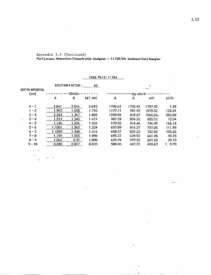
Appendix 3.4 (Continued) Port l~v~~: Ammonium Cono~ntntion An~1y~~ -- 11 /29/84 S~dirMnt Cor~ ~mplo~

DILUTION FACTOR: _ .... _ ... _ .. JJL DEPTH INTERV N..

(em) - - - - - - - - -00640- - - - - - - -

0-1 1 - 2 2-3 3-4 4-5 5-6 6-7 7-8 8-9 9-10

A B NET AVE

2.835 1.792 1.808 1.421 1.323 1.224 1.216 1.098 1.008 0.820

----------------~g-atmN----------------

A B AYE ±STD

1706.6~ 1708.43 1707.53 1.28 1117.11 981.93 1079.52 138.01 1359.04 818.67 1088;861 382.09 907.23 804.22 855:72 72.84 679.52 914.46 796.99 166.13 657.89 816.27 737.08 111.99 658.37 807.23 732.80 105.26 693.37 629.52 661.45 45.15 634.94 579.52 607.23 39.19 500.00 487.35 493.67 i. 8.95

3.52

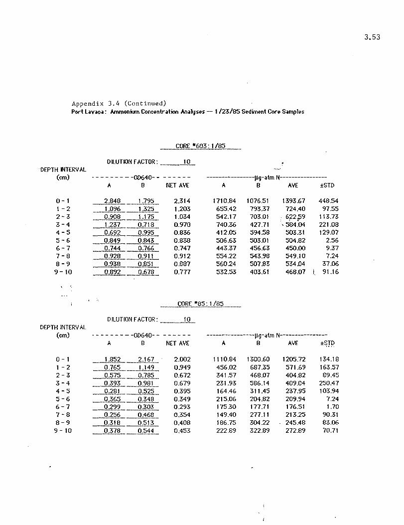
3.53

Appendix 3.4 (Continued) Port l~v~o~: .vnmooium Conc~ntr~tion Anal1,lS(>s -- 1/23/85 Sediment Core S~mples

. __ .... _~gL~§.9.~.~l!.?;? .. _._ ..

DILUTION FACTOR: __ . ___ ..J.!L DEPTH INTERV Al

(em) - - - - - - - - -00640- - - - - - - - ----------------~9-atmN----------------

A B NET AVE A B AVE ±STD

0-1 _~"?j!L _._ .. _L?2L 2.314 1710.84 1 076.51 1393.67 448.54 1 - 2 ... ___ LQ2!?._. __ L.~6;?' __ 1.203 655.42 793.37 724.40 97.55 2-3 ___ . .Q.:2Q.L __ 1 ·.L7.;L 1.034 542.17 703.01 6'f2~9 113.73 3-4 __ L6;?L. _ .. _._Q.:IUL 0.970 740.36 427.71 ,584.04 221.08 4-5 _. __ Q"!?2L __ O.:22L 0.836 412.05 594.58 503.31 129.07 5-6 _ .. _CL?1L _\L?1L 0.838 506.63 503.01 504.82 2.56 6-7 ___ 9..:.1-1L -9.:.7.§L 0.747 443.37 456.63 450.00 9.37 7-8 ___ Q.J_~L .. __ ... Q.,2tL 0.912 554.22 543.98 549.10 7.24 8-9 __ Q.,93L __ OJ~5L 0.887 560.24 507.83 534.04 37.06 9 - 10 _-....9.?2L __ O..:§J!L 0.777 532.53 403.61 468.07 i 91.16

, -.

D flUT ION FACTOR: __ .. _ .... _ ... ..!.Q .... DEPTH INTERV AL

(em) - - - - - - - - -00640- - ------ ----------------~9-dtm N----------------A B NET AVE A B AVE ±~;rp'

0-1 __ ... _L§~) ____ .. ?J!??.._ 2.002 1110.84 1300.60 1205.72 134.18 1 -2 __ q.:It?;? __ . __ LJ.1L 0.949 456.02 687.35 571.69 163.57 2-3 _._Q~~l;?_ ... ____ Q.:1?;?._. 0.672 341.57 468.07 404.82 89.45 3-4 __ ..... .9.:~_~L _ ....... Q.:2?.1. .... 0.679 231.93 586.14 409.04 250.47 4-5 __ ._JL~?.L _. __ .. Q.:;?'~;?'._ 0.395 164.46 311.45 237.95 103.94 5-6 __ .... _Q.,;?§;L __ ._.Q.:~_1L 0.349 215.06 204.82 209.94 7.24 6-7 ___ ..9..:£2L _._.Q.:;?'QL 0.293 175.30 177.71 176.51 1.70 7-8 ___ Q.:6;?'L ___ .9.:1§L 0.354 149.40 277.11 213.25 90.31 8-9 __ q";?,1L_Q:;?JL 0.408 186.75 304.22 245.48 83.06

9 - 10 __ Q";?'lL ___ ... Q";?'1L 0.453 222.89 322.89 272.89 70.71

3.54

Appendix 3.4 (Continued) Port Lavaca: A(nmonium Concentntion Analyses - 1/23/85 Sediment Core Samples

DILUT ION fACTOR: ....... _._ .. __ -'-9 ... . DEPTH INTERY AL

(em) - - - - - - - - -OD640- - - - - - -- ----------------~g-atm N----------------A B NET AYE A B AYE fSTD

0-1 __ .. _ ... LIliL. _J..J.~;?'._ 1.448 1030.12 713.86 871.99 223.63 1 - 2 _____ q.:f.6;? ____ I ·1~~_ ... 0.823 130.72 86024 495.48 515.85 2-3 ____ .JLtQL __ 0_M2._ 0.367 56.02 386.14 2~1.Q8 233.43 3-4 .. _. __ t;!.:Q~.L ___ .J1:1.Q~L 0.242 50.00 240.96 '145.48 135.03 4-5 ____ .Q"?_Q;?_ .. _QJJH .. _ 0.487 480.12 106.02 293.07 264.53 5-6 _ .. __ Q, I OL __ O..J.]§_ 0.134 60.84 100.60 80.72 28.11 6-7 __ ... Q..9.L 0.11L 0.109 49.40 81.33 65.36 22.58 7-8 _J;!.:Q~L _.QJ.1.L 0.114 54.22 83.13 68.67 20.45 8-9 __ 0.1 OL __ ..Q.XL 0.103 56.63 67.47 62.05 7.67 9- 10 __ Q.J.f.;? ___ OJiL 0.114 70.48 66.87 68.67 i. 2.56

DILUTION r ACTOR: .................... 1.9 ... . DEPTH INTERY AL

(ern) - - - - - - - - -OD640- - - - - - - - ----------------~9-atrn N----------------A B NET AYE A B AYE iSm.

0- I "DIY/O! -4.82 -4.82 -4.82 0.00 -_ .. _.-_._.-.... -._ .. -. __ ............. 1 -2 "DIY/O! -4.82 -4.82 -4.82 0.00 ----_ .. ____ 0._- • ____ • ___ •••....••

2-3 "DIY 10! -4.82 -4.82 -4.82 0.00 _ ... _._-_ .. _ .... __ . _ ..................... _-3-4 IIDIY/O! -4.82 -4.82 -4.82 0.00 ..... _ ..•••••...•.•....... _._--............... 4-5 "DIY/OI -4.82 -4.82 -4.82 0.00 ----.------.--5-6 "DIY/o! -4.82 -4.82 -4.82 0.00 --------.. ------_.-.--6-7 IIDIY/O! -4.82 -4.82 -4.82 0.00 _ .. _----- _._ .. _ ...... _--7-8 IIDIY to! -4.82 -4.82 -4.82 0.00 --------------8-9 "DIY/O! -4.82 -4.82 -4.82 0.00 ..... _--_ .. _.- "'---"-'" 9- 10 !lDIV/O! -4.82 -4.82 -4.82 0.00 _ ..... _----_.-_ .. - -_._-----

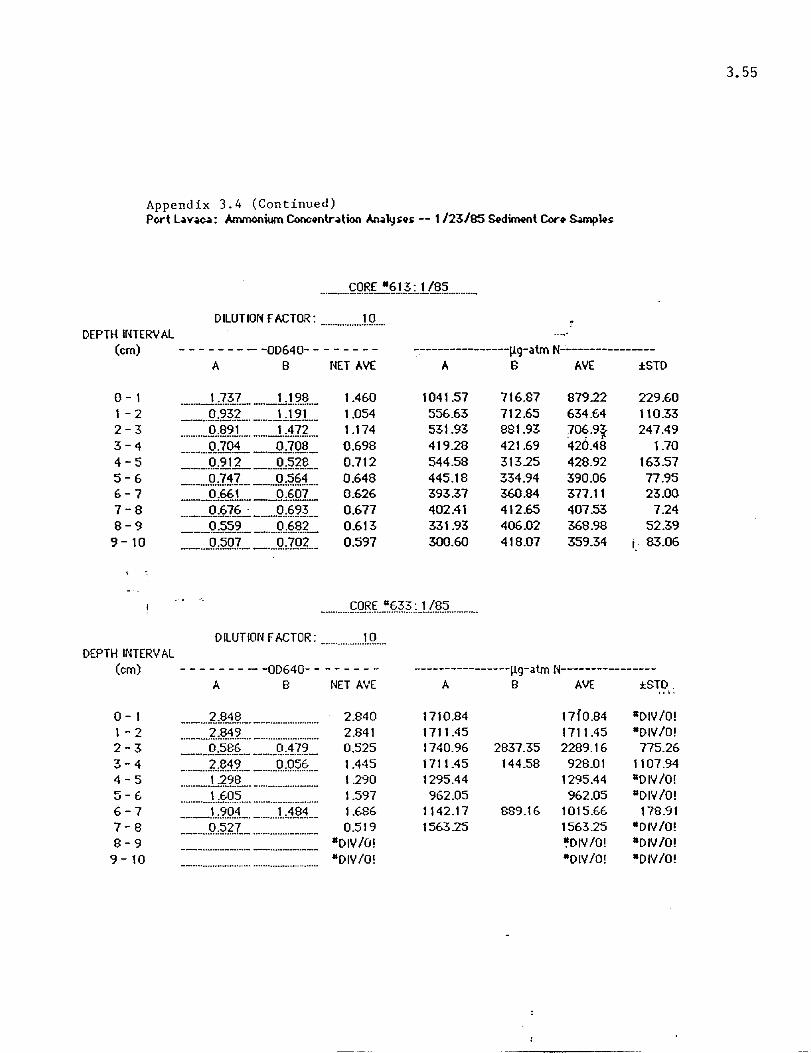
3.55

Appendix 3.4 (Continued) Port L~v~: AIMlonium Conc~ntr~tion An.allJs~s -- 1/23/85 ~dwnt Con S<!mpws

o ILUT ION r ACTOR: _ ..... _ ....... ..1.9._. DEPTH lNTERV AL

(em) - - - - - - - - -00640- - - - - - - - ----------------~9-atmN----------------A B NET AVE A B AVE ±STD

0-1 ____ L.7EL _._L.!.2!L 1.460 1041.57 716.87 87922 229.60 1 - 2 _. __ ... Q"2.~;L. _. __ .. L.L'l.1. .. _ 1.054 556.63 712.65 634.64 110.33 2-3 _ ....... _.Q.:~JL. _._._L1IL 1.174 531.93 881.93 70~.9} 247.49 3-4 _ .. _ ... _Q.7QL _ ... _Q.:19JL 0.698 419.28 421.69 420.48 1.70 4-5 _. __ .Q"911.... _-.Q.:;?'~_L 0.712 544.58 31325 428.92 163.57 5-6 _ ... __ Q.}.1-:L _J!,§§L 0.648 445.18 334.94 390.06 77.95 6-7 __ Q~~J~_1 __ Q~~07 0.626 393.37 ~.84 377.11 23.00 7-8 __ .. _.Q}?J§...;. __ Q.:§2L 0.677 402.41 412.65 407.53 7.24 8-9 ___ Q.,;?~_'L _ ... Q:§?L 0.613 331.93 406.02 368.98 52.39 9-10 __ -.Q~~L _._.Q3.91 .. _ 0.597 300.60 418.07 359.34 i. 83.06

, ,

o ILUT ION fACTOR: _ .............. ..1.Q ...• DEPTH INTERV AL

(em) - - - - - - - - -00640- - - - - - - - ----------------~9-atm N---------------A B NET AVE A B AVE ±STD

I •••

o - 1 _ .. _ .... ?:!;H?.. __ ... ___ ................ 2.84 0 1710.84 17fo.84 "DIV/O! 1 - 2 ...... __ ..?.J!1~ .... _ ... _................... 2.841 1711.45 1711.45 "DIV/O! 2 - 3 ____ .JL:??L _ ...... _9.:1-:1.2- 0.525 1740.96 2837.35 2289.16 775.26 3 - 4 _ ...... _ .. ?:?.12. __ ........ Q.:Q~§ .. _ 1 .445 1711.45 144.58 928.01 1107.94 4 - 5 _ ..... _.U.'!.L _ .... _._ ....... _...... 1 .290 1295.44 1295.44 "DIY/O!

5 - 6 _ ....... _.L§Q:5, .... _ ... _.................... 1 .597 962.05 962.05 IIDIV/O!

6 - 7 _ ... _L'!.QL _ ........ Li?_L 1 .686 1142.17 889.16 1015.66 178.91 7 - 8 _. __ .... Q:;?~L ....... _ ...... _........ 0.51 9 1563.25 1563.25 "DIV/O! 8 - 9 "DIV/O! ~DIY/O! IIDIY/O! 9-10 "DIV/O! "DIV/O! "DIV/O!

Appendix 3.4 (Continued) Port L~v~o~: Anvnonium Cooo~Otr~tiOll An~1lJ!;t'!; -- 1/23/85 St'dimt'ot Cor~ S~mplt'!;

DILUTION fACTOR: _. ___ .. .1.Q .... DEPTH INT£RVAL

(em) . - - - - - - - -OD640" - - - - - - .. A B NET AVE

0-1 _ .. _1)~1L _ .. _~,§~_ .. 2.842 1 - 2 ..... __ f)~L .......... f.:.L!?~ .... 2.497 2-3 .. _ ... f.,~ .. ~ .. _ .. _f.~;?'iL 2.512 3-4 _ ... _L!?2!L __ 1 :§78 . 1.779 4-5 _U.'?!L __ l~§L 1.526 5-6 __ .LLHL .. _ .. ..L.~;:!!L 1230 6-7 .......... L.1.QL _Q.1§',L 1.027 7-8 _ .... Q)~.1.L .. _LQ~L 0.963 8-9 __ O"lH!L --.Q§.? .. 'L 0.751 9- 10 __ .. Q.~'?QL -..-Q,~1;:! .... 0.781

DILUTION fACTOR: .... _ ........... ..!.Q .. .. DEPTH INTERY AL

(em) . - - ........ - "00640- - - - - - - -

0-1 1 - 2 2-3 3"4 4-5 5 .. 6 6-7 7-8 8-9 9-10

A B NET AYE

... _ .. .J..,~~_ ....... _1 .4 .. ~?..... .

.. __ ................. __ ?..:.f.~!L

_ ..... f.,~~ .. !L .. _ ....... _._ .... . ....... _L2!?1. ... _ .......... __ ....... . .. _ .. _L~Q!L __ ... _ ...... _. __ ... f)?11..... .. ___ .

1.316 2.230

"DIY/O! 2.390 1.959 1.500 2.839

"DIV/O! "DIY/O! "DIY/O!

-------.. ---.. ----~g-atmN-...... - .. -------...... A B AVE ±STD

1711.45 1712.05 1711.75 0.43 1712.05 1295.78 1503.92 294.34 1496.39 1529.52 15.12~5 23.43 1016.87 1126.51 '\071.69 77.53 837.35 IODO.60 918.98 115.44 668.67 81325 740.96 10223 661.45 575.30 618.37 60.91 505.42 654.82 580.12 105.64 487.95 41627 452.11 50.69 538.55 401.81 470.18 i 96.69

- .... --------.. - ...... ~g .. atmN .......... - .. --.......... - ..

A B AVE ±~JP

1808.73 861.45 1335.09 669.83 1343.37 1343.37 "DIY/O!

"DIY/O! "DIY/O! 1439.76 1439.76 "DIY/O! 1180.12 1180.12 "DIV/O! 903.61 903.61 "DIY/O!

2137.80 2137.80 "DIY/a! "DIY/O! "DIY/O!

."DIY/O! "DIY/a! ·DIY/O! ·DIY/O!

3.56

3.57

Appendix 3.4 (Continued) Port L~v~o~: Poro 'w'~t.r Ammonium Conoootntioo -- '6lblas S<>d;moot Con S=>p~"

DILUTION FACTOR: _. __ ..J.Q .... DEPTH INTERV At

(em) . - - - - - - - -OD640- - - - - - - - ---------\19-atm Nil of Pore V"ter--------A B NET AVE A B AVE ±STD

0-1 __ ]§4L_~·793_ 2.659 1525.90 1677.71 1 b01.81 107.34 1 - 2 ---1211- __ ._U1L 1.809 1150.00 1028.92 1089.46 85.62 2-3 __ I_.4_R- __ 1_.£~ 1.316 854.82 730.72 792.77 87.75 3-4 . ____ L~OL ___ L.L~~L 1.243 780.12 716.87 . 748.~9 44.73 4-5 __ I_·o.QL __ O.:2~L 0.964 601.20 559.64 580.42 29.39 5-6 _0.982 ___ 9.Jl~L 0.928 586.75 530.72 558.73 39.62 6-7 __ 0.178 _9.:.I!.L 0.740 463.86 427.71 445.78 25.56 7-8 __ 1·9.1L_(L1Q:L. 0.867 625.30 41928 52229 145.68 8-9 ____ 0.7~_L __ O..:§~ .... 0.645 457.23 319.28 388.25 97.55 9-10 _9.:61.!L _._QJ_Q.L 0.654 367.47 420.48 393.98 i 37.49

.... _ ...... __ ... ~QRL~?!?~§t~~L .......... .

D ILUT ION FACTOR: __ .............. .!.Q ... . DEPTH INTERV AL

(em) . - - - - - - - -OD640- - ------ --------\1q-atm Nil of Pore Y/ater---------A B NET AVE A B AVE ±STD

;;\ :

0-1 _._ .. _;U!1:L _._L1~;?' .... 2.641 1708.43 1472.89 1590.66 166.55 1 - 2 _ .... .1:1.1.1-.. _t~~L. 1.475 846.99 929.52 883.25 58.36 2-3 _. __ \MIL _ . ...Q.?iL 0.599 280.12 441.57 360.84 114.16 3-4 __ ._.9.:12L _ .. _JU_'?_L 0.605 252.41 475.90 364.16 158.03 4-5 _._9);).9_L _.Q:H~_ .. 0.329 31.93 363.86 197.89 234.71 5-6 __ ... _9.J_~f>_. _____ 9.·4 ""(L 0.607 450.60 280.12 365.36 120.55 6-7 _(t;?'1L_Q~;?'~L 0.542 322.29 330.72 326.51 5.96 7-8 _ ... _Jt2L __ 9.:!?~L 0.709 543.37 3\0.84 427.11 164.42 8-9 _._I.:.Q?_L _Q."~~!L 0.951 645.18 500.00 572.59 102.66

9 - 10 _U.f>J __ L11L 1.281 694.58 848.80 771.69 \09.05

3.58

Appendix 3.4 (Continued) Port l~v~o~: Por .. W'~t"" Ammonium Cooo"ntr~tion - l/6/as S"dim"nt Con S~mpl .. ~

DILUTION FACTOR: .. _. ____ .HL DEPTH INTERVAL

(em) - - - - - - - - -00640- - - - - - - - ---------\-lg-.;tm 1'111 in Pore 'w'ater---------A B NET AVE A B AVE ±STD

0-1 __ ._(LI!?L __ !).,!?QI._ 0.680 45B.43 360.84 409.64 69.Q1 1 - 2 _ .. _._'I,;UL . __ ._ .. \tI~L 0.627 306.02 448.80 377.41 100.95 2-~ _.~~;? ___ Q.}_~L 0.2Bl 141.57 196.39 16B.98 3B.76 3-4 __ .. _J1.,fQ~L _. __ .Q.,H§ __ 0.182 117.47 101.20 1.D9.34' 11.50 4-5 ___ .. _Q~~QL __ ... _9JEL 0.175 117.47 92.77 105.12 17.46 5-6 _._OJ}L.~~?L 0.252 77.71 225.90 151.Bl 104.79 6-7 ___ 0.1..12.... ~.2;?_ 0.099 66.87 52.41 59.64 10.22 7-8 _. ___ U1L _.Q .. 12_~ __ 0.112 65.66 68.67 67.17 2.13 B-9 __ .Q.:.L1L_~JJ.L 0.107 63.25 65.06 64.16 1.28

9 -10 ._._O..JJ.L _____ 0.105 63.25 0.00 0.00 i 0.00

, ,

D ILUT ION FACTOR: __ .... _ ........ ..19 ... . DEPTH INTERVAL

(em) - - - - - - - - -00640- - - - - - - - ---------l1g-dtm 1'111 of Pore W"t~r--------A 8 NET AVE A 8 AVE ±STD

0- 1 _ ..... _ ... L?;?:L ...... _ .. .9.,2?:L 1.336 1039.76 569.88 804.82 ~.32.25

1 -2 ............ L:?..?.;?_ ... __ .. _ .. L.L~L 1.227 762.05 716.27 739.16 32.37 2-3 _._ .. .9.,2.!.?._. ___ ._LQ.1.;?' .. _ 0.957 546.39 606.63 576.51 42.60 3-4 _ ......... .9.,lQ§ .... ......... .9.,§I2 .... 0.686 421.69 404.22 412.95 12.~5

4-5 __ ._ ... Q.,?§L __ Q.~?.1.L 0.584 334.94 368.D7 351.51 23.43 5-6 __ .Q~;?'§?' ____ . __ LQilL 0.699 215.06 626.51 420.78 290.94 6-7 _. ____ .Q~;?JlL ._.....Q.,;?_~lL 0.420 lB6.75 319.28 253.01 93.71 7-8 _ ... __ !).}fL _. __ Q~'!L 0.398 189.16 290.36 239.76 71.56 8-9 ___ .Q.:.?2;?'. ____ .Q.~'!1L 0.363 172.B9 263.86 21B.37 EA.32

9 - 10 _ ....... _.Q.B;?_. __ .. ..Q.,i~L 0.426 221.08 291.57 ·256.33 49.84

3.59

Appendix 3.4 (Continued) Port Lavaca: Port' 'Iatt'r Ammonium Conct'ntration -- 3/6/B5 ~dimt'nt Con S.mplt's

_ ... _ .... ~Qgt.~.§H .. ~.~.t.?;i ........ __

D ILUT ION fACTOR: ___ ... ..1.Q •• _ DEPTH INTERVAL

(em) - - - - - - - - -OD640- - - - - - - - ---------I1q-atm NIl in Pore W'ater---------A B NET AVE A B AVE r' ±STD

0-1 __ IA~.L ___ J..:~lJ?' .. _ 1.523 859.04 975.90 917.47 82.64 1 -2 . __ J_:J.~_L _t61 L 1.377 690.36 968.67 829.52 196.80 2-3 __ 0_.~99 1.276 0.980 41627 763.B6 590.06 245.78 3-4 __ 0.7iL _1..:.1.9.L 0.915 442.17 660.24 551.20 154.20 4-5 __ Q.7~_1 __ UJ.L 0.941 5-6 __ O~B4.L __ I·?i~.L 1.094

465.66 667.47 566.57 142.70 505.42 B12.05 658.73 i 216.82

6-7 , __ 0·9QL~2:L 1.140 , 537.95 834.94 686.45 210.00 7-8 __ (L?IL __ 1 J?iL 0.996 521.08 678.31 599.70 111.18 8 ':9 ~ __ ::..QJ347 _____ J.J.g._ 0.982 9- to; ___ .Q.:.t?1L __ LQ~;L 0.830

505.42 677.71 591.57 121.83 381.33 618.67 500.00 157.83

.;1.

3.60

Appendix 3.4 (Continued) Port l..,v..,o..,: Pon 'vI ... t~r Ammonium Cono~ntr..,tion -- 3/6/85 S~dim~nl Con S..,mpl~s:

_ .. ___ ... g}E.L~1;?'.; .. ;'i.f..?':J .......... __ .

DILUTION FACTOR: __ .......... __ .1.Q ...• DEPTH "HER'¥' AL

(ern) . - - - - - - - -OD640- - - - - - - - ---------l1g-alm NIl of Por~ 'w'"lt'r--------A B NET AVE A B AVEt· tSTD

0-1 _L~;?'~L ___ f~;?2?_ .. 1.957 919.88 1437.95 1178.92 366.33 1 - 2 _1..}49 __ 1.5~L 1.643 1048.80 930.12 989.46 83.92 2-3 1.467 1.1~L 1.303 878.92 690.36 784.64 133.33 3-4 __ 1·11:L __ l·i?L 1.596 1066.87 856.02 961.45 149.09 4-5 2.~_1.t?._ 2.838 1709.64 1709.64 OIDIV/OI 5-6 _~Jl1L_.f.J 9L 2.514 1710.24 1318.67 1514.46 i.276.88 6-7 "DIV/O! -4.82 -4.82 -4.82 0.00 -------- -_ .... __ ... __ .-, , 7-8· #DIV/O! -4.82 -4.82 -4.82 0.00 ------------ _ .......... __ ......... 8-=9 .. '~ _ ... __ .. _--- - ...... -.------- IIDIV/O! -4.82 -4.82 -4.82 0.00

9 - 10; IID1V/0! -4.82 -4.82 -4.82 0.00 _._ ... _ ....... _ ... - ...........................

Appendix 3.4 (Continued) Port l~v~o~; PorQ ..... ~tQ,. Ammonium ConcQntr~tion -- 4/3/85

D U.UTlON fACTOR: __ .. _ .. 1.Q. ... DEPTH INTERV Al

(em) - - - - - - - - -OD640- - - - - - - - ---------l1g-atm 1'1/1 of Por(' W'ater--------

0-1 1 - 2 2-3 3-4 4-5 5-6 6-7 7-8 8-9

9 - 10

DEPTH INTERV AL (em)

0- 1 1 -2 2-3 3-4 4-5 5-6 6-7 7-8 8-9 9- 10

A B NET AVE A 8 AVE ±STD

___ L?.IL __ .WIL 1.317 942.77 643.37 793.07 211.71 _ .. __ L.t?:L. _. __ ..!t§;!:? .. _ 0.980 672.29 508.43 590.36 115.86 _. __ .Q.:!~~~L ___ L91'_L 0.946 510.24 628.92 569.58 83.92 _ .... _.Q.:§:?§ .... _ .. _...Q"~§'L 0.890 492.77 578.92 535.84 60.91 __ Q.:74L ._Q':!JL 0.740 445.18 445.78 445.48 0.43 __ Q.:!?.1;?'._. _ ........ Q.:?J.L 0.672 382.53 426.51 404.52 31.10 _ . .9·qL __ 0.5~L 0.601 369.88 353.61 361.75 11.50 ___ ...Q."~J.~L __ .....Q.§?L 0.639 368.07 401.20 384.64 23.43 __ J).:;!L __ (H!~L 0.599 332.53 388.55 360.54 39.62 ___ Q.:fd;? .... __ .. Jt~?L . 0.607 382.53 348.19 365.36

i 24.28

_._ ... _ .... ~.Q.~I .. ~?;:;.;_1f..?;i .... __ ..... .

DILUTION fACTOR: ............... _ .. !.Q ... .

. - - - - - - - -OD640- - - - - - - - ---------l1g-dtm 1'111 of Pon' 't(at~r---------A B NET AVE A 8 AVE ±STD

___ .L;??:?_ .. _. ___ L?_'?L 1.531 827.71 1 016.87 922.29 133.75 . ___ .J..:;?''!.1 .. ____ .. J..:Q~~_ ... 1.166 786.75 617.47 702.11 119.70 _ .. _ . .Q.:~fg .......... _Q.~1Q:L 0.484 345.78 237.35 291.57 76.67 __ .. _.Q.:1~.! ... _ ._ .. _ ... Q.,;?.!.1 .... 0.376 333.58 465.36 399.47 93.18 __ !P~L _ .. __ q";?'~_L 0.304 172.89 193.37 183.13 14.48 ____ .. Q.:1L __ .. _!M.1.!:! .... 0.406 242.17 246.99 244.58 3.41 _._ .... Q.:1;?.1.. ... __ .. _.Q.:2IL 0.347 254.82 162.65 208.73 65.17 _. __ q.,;??:? .. ___ ...... Q.::£1.1..._ 0.304 225.30 140.36 182.83 60.06 __ .. Q.::?'?J ____ ... Q."?:?';?_ 0.247 166.27 130.72 148.49 25.13 _ .. _O_BL .. _ ... _.Q.';?'§~ .... 0.312 162.05 213.86 '187.95 ~6.63

3.61

3.62

Appendix 3.4 (Continued) Port L~vac~: Pore Vater Ammonium Concentration -- 4/3/85

......... _ .. ~.Qg.L~§;?; .. 1.f..?..~ ..... _ ...... _

DILUT ION FACTOR: .............. __ J_Q._. DEPTH INTERV AL

(em) - - - - - - - - -00640- - - - - - - - ---------~9-atm Nil of Port' \v'ater--------A B NET AVE A B AVE tSTD

0- 1 _ ... __ Q"Q!?'?_ ... _ .. _...Q,.~1L 0.345 32.53 382.53 207.53 247.49 1 -2 __ . ___ LQ~;;; .... __ .LQJ.L 1.045 653.61 604.82 629.22 34.50 2-3 .. _ .. __ L~?J __ L1~L 1.386 809,04 860.24 834£)4- 36.21 3-4 .. _ .. _.Q"~I':L ___ JL~_~_ 0.809 581.93 392.17 4~7.0S . 134.18 4-5 _._._, ·~L __ .P-~1J.L 0.814 737.35 243.37 490.36 34929 5-6 _. ___ It§§L _Q.,.?11_ 0.443 393.37 140.36 266.87 178.91 6-7 ____ P-JJ1_L _O.~ 0.452 422.29 12229 272.29 212.13 7-8 __ ._ .. Q.,.l?!? __ . _ltL!?L 0.462 468.67 87.35 278.01 269.64 8-9 _._Q":?.LL _Q~.1.?JL 0.181 127.11 90.36 108.73 25.98 9- 10 ___ !LL~!? ___ .QJ.?!L 0.164 88.55 108.43 98.49 I 14.06

........... J~Q~~ ...... t;.f.~ .. ;.1/13.;? ............ .

DILUTION FACTOR: _ .. _ ........... ...1.Q .. _ DEPTH UHERV AL

(em) - - - - - - - -- -00640- - - - - - - - ---------~9-atm Nil of Pore \v'ater---------A B NET AVE A B AVE tST.!? .

0 - 1 ............ L~?:?L _._ ..... L12§ .. _ 1 .679 944.58 1078.31 1011.45 94.56 1 - 2 __ ........ LQ;?L __ .... ..!..P_'!.L 1.071 633.13 656.63 644.88 16.61 2- 3 _. __ .... Q.,~~.L. . .. _ ..... Q.,~_'!.L 0.967 568.07 596.39 582.23 20.02 3- 4 ... ___ . __ Q.,§L __ . __ .Q .• ~QL 0.754 921.69 539.76 nO.72 270.06 4 - 5 _ .. _q.:I?? .. ___ . __ Q.~?~.L 0.773 433.73 497.59 465.66 45.15 5-6 . __ .. _.Q.:~lL .. _._Q"~t7..L_ 0.891 553.61 519.88 536.75 23.85 6- 7 _ .... _._Q.:~?} _ ___ q.k.2L 0.818 571.69 413.25 492.47 112.03 7- 8 .. __ ... Jt~§L __ .. _ .. Q";?§L 0.416 831.33 334.34 582.83 351.42 8- 9 ___ (L~?_L __ (t7.fa._ 0.552 1039.16 457.23 ·748.19 411.49 9- 10 ._ ... _. ___ ._ ...... __ ... Q.:;?'~L 0.586 -4.82 353.01 174.10 253.02

Appendix 3.4 (Continued)

Port L~v~c~: Por9 ..... ~t9r Ammonium Cono~ntr~tion -- 4/3/85

__ ._~Q~f; ... ~§.!.~.: 4 !.!:l~ ... _._ ...

DILUTION fACTOR: ._._._ . ..!!L DEPTH UHERVAL

(em) - - - - - - - - -OD640- - - - - - - -A B NET AVE

0-1 _. __ .. ..L;??L _I!:~~_ 1.267 1 - 2 __ .. JlnL ___ Q.:?.2L 0.896 2-3 __ O.J~73 ____ QJmL 0.878 :5-4 _ .. 93LL._~I67 __ 0.732 4-5 __ 0.864 ___ Q,?04 . 0.726 5-6 0.8f.L _C)~gtL 0.745 6-7 __ O.:1~L_.Q]§L 0.621 7-8 __ O.d.Q~L _Q.,l~L 0.607 8-9 0.571 -.-!l1QL. 0.628 9-10 ___ 0·I1L _-9..:.~;?'L 0.643

D ILUT ION FACTOR: _._. __ . ..1Q .. _ DEPTH INTERVAL

(em) - - - - - - - - -00640- - - - - - - -

0-1 1 - 2 2-3 3-4 4-5 5-6 6-7 7-8 8-9 9- 10

A B

_ .. _ .. _ ... _. __ ._ ... _ .. _.J..:1~1 .. _ _ .. _ .. __ ... _. __ . _ ... _.l.:1.Q;? .. _ __ ........ L~§;? .... ____ ._ .. _ .... _._ _. ___ Q.::?Q~L _._gJ.1L _ .. _ ... _Q.:J.9_L _ .. _ .... _ .... _ ._ .. __ QJ~j_!L _ .. ___ .. _ .. _. __ .. _ ... LL!?L _ ...... ___ _ ---?"~~~- ---_ ... _--__ ._1 .§~~. ___ ._. __ .. _

NET AVE

1.786 2.397 1.255 0.420 0.698 0.840 1.144 2.251 1.650

#DIY/O!

--------Ilq-atm 1'111 of Por~ ..... ater---------A B AVE iSTD

939.16 SB7.35 763.25 24B.77 546.99 532.53 539.76 10.22 521.08 536.14 52.8.~J 10.65 424.10 457.23 440.66 23.43 515.66 359.04 437.35 110.75 490.96 406.02 448.49 60.06 294.58 453.61 374.10 112.46 301.81 429.52 365.66 90.31 339.16 417.47 37B.31 55.38 444.58 330.12 387.35 i 80.93

---------Ilg-atm 1'111 of Por~ Water---------A B AVE iSm.

1793.53 1793.53 #DIV/O! 1443.98 1443.98 #DIV/O!

756.02 756.02 #DIV/o! 422.29 4186.75 2304.52 2661.87 420.48 420.48 #DIV/O! 506.02 506.02 #DI'v'/O! 689.16 689.16 ilDIV /O!

1356.02 1356.02 -DIV/o! 993.98 ·993.98 -DIV/O!

ilDIV to! ilDIY/O!

3.63

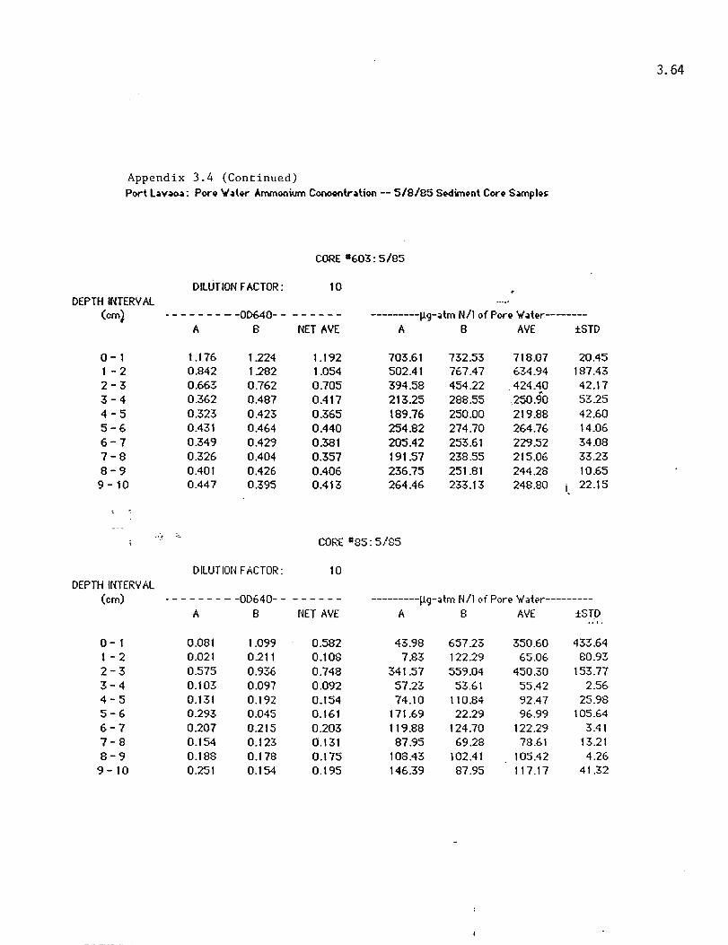
3.64

Appendix 3.4 (Continued) Port l .. v .. ~: Pon 'vI .. t~r Ammonium Cooo~ntr .. tion -- 5/8/85 S~im9nt Con S .. mpl~s

CORE 11603: 5/85

DILUTION FACTOR: 10 DEPTH INTERV Al

(em) • - - - - - - - -OD640- - - - - - - - ---------l1g-.. tm N /1 of Pon 'vI .. t~r--------A B NET AVE A B AVE iSTD

0-1 1.176 1.224 1.192 703.61 732.53 718.07 20.45 1 - 2 0.842 1.282 1.054 502.41 767.47 634.94 187.43 2-3 0.663 0.762 0.705 394.58 454.22 424.40 42.17 . 3-4 0.362 0.487 0.417 213.25 288.55 . 250.90 53.25 4-5 0.323 0.423 0.365 189.76 250.00 219.88 42.60 5-6 0.431 0.464 0.440 254.82 274.70 264.76 14.06 6-7 0.349 0.429 0.381 205.42 253.61 229.52 34.08 7-8 0.326 0.404 0.357 191.57 238.55 215.06 33.23 8-9 0.401 0.426 0.406 236.75 251.81 244.28 10.65

9 - 10 0.447 0.395 0.413 264.46 233.13 248.80 i 22.15

CORE 1185: 5/85

DILUTION FACTOR: 10 DEPTH INTERVAL

(em) • - - - - - - - -OD640- - ------ ---------l1g-atm N /1 of Por~ 'vi at~r---------A B NET AVE A B AVE iSTD

0-1 0.081 1.099 0.582 43.98 657.23 350.60 433.64 1 - 2 0.021 0.211 0.108 7.83 122.29 65.06 80.93 2-3 0.575 0.936 0.748 341.57 559.04 450.30 153.77 3-4 0.103 0.097 0.092 57.23 53.61 55.42 2.56 4-5 0.131 0.192 0.154 74.10 110.84 92.47 25.98 5-6 0.293 0.045 0.161 171.69 22.29 96.99 105.64 6-7 0.207 0.215 0.203 119.88 124.70 122.29 3.41 7-8 0.154 0.123 0.131 87.95 69.28 78.61 13.21 8-9 0.188 0.178 0.175 108.43 102.41 105.42 4.26 9-10 0.251 0.154 0.195 146.39 87.95 117.17 41.32

3.65

Appendix 3.4 (Continued) Port L .. V;lO .. : Por~ W;lt~r Ammonium Cono~ntr;ltion -- SIBIBS

__ .. __ .. £Q~_~~~.;.;!!.!;l~ .... _ .. _._

DILUTION FACTOR: _._._ .. _ ........ UL.. DEPTH INTERVAL

(em) - - - - - - - - -00640- - - - - - - - ---------Ilg-atm NIl of Pore Water--------A B NET AVE A B AVE :l:STD

0-1 _ ... __ I·!.~L _.~t54L 0.894 752.41 324.10 538.25 :!'-O2.86 1 - 2 __ .... 9.~~?.L. __ 1..:??1... .. 0.943 405.42 130.72 568.07 2W.02 2-3 __ 9"~;?'?' _ _ Q,.n;L 0.559 210.B4 462.05 336.45 177.63 3-4 __ . __ 9.,fZL __ O.,~.t9.~L 0.338 129.52 277.71 203.61 104.79 4-5 __ 0.,~78. __ Jtf~~._. 0.311 222.89 151.20 187.05 50.69 5-6 __ .. ..Q,~.L_(U§_!2_ 0.202 148.19 94.58 121.39 37.91 6-7 __ QJ2L __ 0..:H_L 0.128 68.67 84.94 76.81 11.50 7-8 __ 9)95 -..!!J.QlL 0.094 52.41 6024 56.33 5.54 8-9 0.102_ O.1QL 0.094 '56.63 56.02 56.33 0.43 9- 10 _-.9..:9]L __ !L09L 0.076 40.96 50.60 45.78 6.82

. ,

DILUTION FACTOR: ___ .. _ ....... --'.9 .. _ DEPTH UHERV AL

(em) - - - - - - - - -00640- - - - - - - - ---------Ilg-atm NIl of Pore Vater--------A B NET AVE A B AVE ±STD

0-1 ___ .Q"§!.:L __ .Q)~!.!L. 0.720 372.89 493.98 433.43 85.62 1 -2 .. __ .. _9.,1~1 .... _ ... __ Q.,~lL 0.875 473.49 580.12 526.81 75.40 2-3 _._. __ .. Q~?.1.L __ O,z"§.? ... 0.766 486.75 436.14 461.45 35.78 3-4 _. __ ... .Q.}2?i ____ .Q.,;?;?.L 0.664 472.89 327.11 400.00 103.08 4-5 ._._Q";?QL __ Q.,;?QL 0.496 300.60 296.99 298.80 2.56 5-6 .. _ .... _Q.,~~L ____ Q-'-!2~L 0.445 197.59 337.95 267.77 99.25 6-7 _._Q"~1.L __ Q":!Q§ .. _ 0.367 202.41 239.76 221.08 26.41 7-8 . ___ .... ~t;?.!.L ____ Q.,;??;?._ 0.441 303.61 227.11 265.36 54.10 8-9 ._ ... __ 9..,;?fL __ .Q";?_~L 0.410 304.22 189.16 246.69 81.36 9- 10 _. ___ ~t§:!L ____ (l,;?lL 0.434 384.94 137.95 261.45 174.65

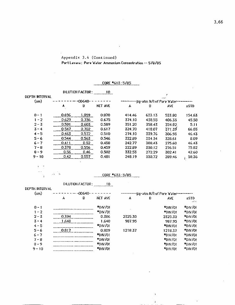
3.66

Appendix 3.4 (Continued) Port l~v~c~: Por~ YI~tE'r Ammonium Cono(>ntr~tion -- 5/s/s5

___ ~OR~ .. ~.§H.; .. ~!.!:!~ ..... __ _

DILUTION FACTOR: .... _ ....... _--1.9_ .. DEPTH INTERV Al

(em) - - - - - - - - -OD640- - - - - - - - --------l1g-aUn Nil of Pon.> YI ater---------A B NET AVE A B AVE ±STD

0-1 __ .9.:§2.L _._I·~L 0.870 414.46 633.13 523.80 154.63 1 - 2 __ .. __ Q.:!?_~~_. _ ... _ .. Q3;?§ .... 0.675 374.1 0 43S.55 406.33 45.58 2-3 ___ Q"?2.L __ ....9.:§QL 0.589 351.20 35S.43 354.82. 5.11 3-4 .. __ 0"~1J __ _ .9.:19L_ 0.617 324.70 418.07 37U9 66.03 4-5 __ ._9.:1g ____ Q.:?IL 0.510 274.10 339.76 306.93 46.43 5-6 _._C!:;?_44 ___ . ...Q."~§.~._ 0.546 322.89 334.34 328.61 8.09 6-7 __ 0.41 L __ JL~L 0.458 242.77 308.43 275.60 46.43 7-8 __ Q"~}L _£L~'§_ 0.459 222.89 330.12 276.51 75.82 8-9 --_Q"~p 0.4t? __ 0.502 332.53 272.29 302.41 42.60 9-10 ____ Q"iL __ O:;?~L.. 0.481 248.19 330.72 289.46 i 58.36

.......... _~Q~L~.§.~.;'i .. :._~!.?;? ........... .

DilUTION FACTOR: .... _ ............ 1.Q. .. . DEPTH UHERVAl

(em) - - - - - - - - -OD640- - - - - - - - ---------l1g-aUn NIl of Pore Water---------A B NET AVE A I:: AVE ±STD

0- 1 ........................ _ ... _ .. __ .... -........... IIDIV/O! IIDIV/O! IIDIV/O! 1 -2 ....... _ .... _ ..............•.....•.•..•.•.. _._ ...... IIDIV/O! IIDIV/O! "DIV/O! 2-3 .. _ ... _Jt2?1 .. __ ....... __ ......... __ 0.386 2325.30 2325.30 "DIV/ol 3- 4 ............ L§1? .... _ .. _._ ... _ ...... _ ..... 1.640 987.95 987.95 IIDIV 10! 4- 5 IIDIV/ol "DIV/O! "DIV /O! _ .... _._ .. __ .......... _ •.•... _ .... __ ...... 5-6 _ .. _ .... _Q.:?J.I __ . __ .. _ ... _._ ..... 0.809 1218.37 1218.37 IIDIV/O! 6-7 IIDIV/O! "DIV/O! "OIl,' 101 _._ .............•...• _-- -.......... --.... --7- 8 IIOIV/O! 110 IV 10! coOIV 10! -_ .... _ .......... _._ .. - -_ .... __ ........ __ . 8-9 IIDIV/O! IIDIV /O! "DIV/D! ._ .......... _ ... _._- _._._ .... _ .... -9- 10 IIDIV/O! coDIV 10! "OIV/O! _._ .......•..•.......... - _ .......... __ ._._--

3.67

Appendix 3.4 (Continued) Port L.w;oo;o: Poro ,",,,tor Ammonium eonoontr"tion -- 6/5/95

DILUTION r ACTOR: __ . __ .... __ ..1Q._ DEPTH INTERV AL

(em) - - - - - - - - -00640- - - - - - - - ---------l1g-atm Nil o(Pore Water---------A B NET AVE A B AYE ±STD

0-1 ___ Q.:1.?£ ___ ~:.1.~L 0_315 285_54 233.43 259.49 36.85 1 - 2 ___ .... Q.::?;iJ: .... _._(U.;?L O.ISS 150.00 189.76 169.88 28.11 2-3 ___ .o.~_~;?._. ___ Q.:.H~ .. _ 0240 196.99 228_92 212.95 22.58 3-4 __ .-P..:.1.QL ___ QJ.I~ .. _ 0.282 237.35 256.02 ?4~69 13.21 4-5 ___ QJ.?;£ __ ._P'.:.1}L 0-125 74.70 188.25 ... 131.48 90.29 5-6 _ .... _Q"l;?:? .... __ Q:Q1L 0.090 86.75 52_71 69.73 24.07 6-7 _-R.1~!L _ .. _Q-!.I;t9.L 0.153 132.53 129.52 131.02 2.13 7-8 __ \LLIL __ ._Q-!.t;i_'!.... 0-157 10120 219.88 160.54 83.92 8-9 _ .. _.QA~t~L __ QJ.;?'?"._ 0.293 263.25 224.40 243.83 27.47

9 - 10 __ .Q.:1.l~tL __ .Q.:.1.9_t?._ . 0246 236.75 147_59 192.17 63_04

........ _ ..... c;;.Qg.f: .. ~§;;i.; . .§.f..?.~ .............. .

DILUTION FACTOR: ___ ........... JQ ... . DEPTH INTERY AL

(em) - - - - - - - - -00640- - - - - - - - ---------l1g-atm Nil of for.: Yfater----------A 8 NET AVE A B AVE ±STD

;; .. 0- 1 __ ._.9.:£9.1. .... __ ...... P..:;?~;L 0.396 16627 285.16 225.71 84.07 1 -2 .......... Q:.!.I.2 .... .......... Q.::?;?§ .... 0.210 103.01 138.46 120.74 25.07 2-3 _ ....... .9.:.1.Q§ .. __ ....... .9.:?;?:? .... 0.236 59.04 207.69 133.36 105.12 3-4 __ .... ..Q.,QI.;? .... .. _ ..... P..:;?:?? ... 0.191 40.36 174.73 107.54 95.01 4-5 _ ...... Q]?L ___ .P'.:'!:1L 0.249 137.35 150.00 143.67 8.95 5-6 ._ .... _.Q.::?26 .... __ ._.P.]§2 .... 0.273 171.08 145.60 158.34 18.02 6-7 _ ... _.P.":??? .... .... _ ... .Q.::?;?.L .. 0262 168.67 135.71 152.19 23.31 7-8 ._ .... _Q"Q.!.!? .... _ .. _ .. Q.:.L~} .... 0.097 4.82 103.85 54.33 70.02 8-9 __ ._ .. Qn~L __ ... __ ...... _ ... _ .. 0.171 103.01 103.01 "DIY 10! 9- 10 _ ... P.";?;?L __ .. _ .. _ .... _ ... 0.246 148.19 148.19 !IDlY 10!

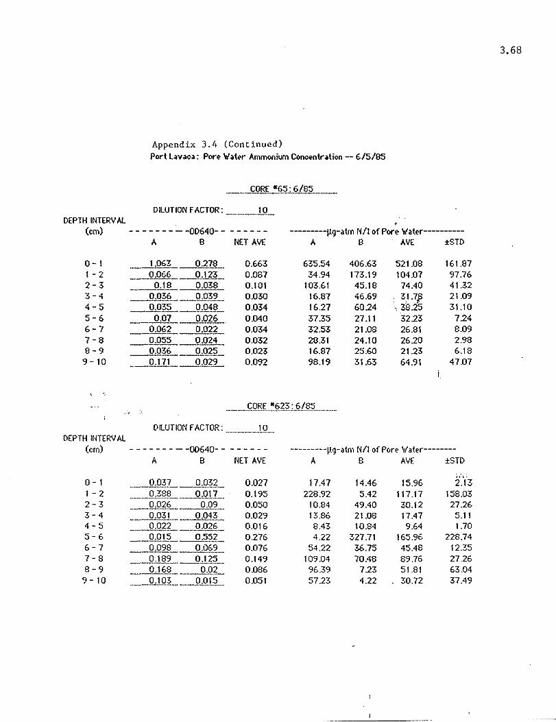
Appendix 3.4 (Continued) Port lavaca: Pore Vat .. ," Ammonium Conoentration -- 6/5/85

... __ ........ ~.Q.~.!§;?.; . .fd.fJ'jJ._ ... __ _

DILUTION fACTOR: _ ......... ___ . .!.!;! .. _ DEPTH INTERV Al ,

(em) - - - - - - - - -00640- - - - - - - - ---------Ilg-atm NIl of Pore Water----------A B NET AVE A B AVE ±STD

0-1 . ___ I.:Q!?1. ___ (L~I? .. _ 0.663 635.54 406.63 521.08 161.87 1 - 2 _._ ... Q"Q~_~_. _. __ QJ_~L 0.087 34.94 173.19 104.07 97.76 2-3 _ .. __ JL1.L _Q.:!2~?_. 0.101 103.61 45.18 74.40 41.32 3-4 ._...Q.:.Q~_L ____ Q"Q~_cL 0.030 16.87 46.69 3,1.7p 21.09 4-5 ___ Q..Q?iL _QJ21L 0.034 16.27 6024 ,3825 31.10 5-6 ___ ... _O·Q:L _.9"91L 0.040 37.35 27.11 3223 7.24 6-7 ___ 9·0§6 __ (W_~L 0.034 32.53 21.08 26.81 8.09 7-8 __ g~_~L_Q.:Q~L 0.032 28.31 24.10 2620 2.98 8-9 _JtQ~6 __ !W?~_ 0.023 16.87 25.60 21.23 6.18

9 - 10 _. __ .. QJ..lL __ q.:Q~L 0.092 98.19 31.63 64.91 47.07

. __ ...... ~Q~~ ... ~.§?~ .. : . .fd?;? ...... __ .. .

Dn.UTlON fACTOR: _ ..... _ .... _._..1.9 .... DEPTH INTERV AL

(em) - - - - - - - - -00640- - - - - - - -

0-1 1 - 2 2-3 3-4 4-5 5-6 6-7 7-8 8-9

9 - 10

A B NET AVE

0.027 0.195 0.050 0.029 0.016 0.276 0.076 0.149 0.086 0.051

---------V-g-atm Nil of Pore \Yater--------A B AVE ±SlO

•• i.

17.47 14.46 15.96 2.13 228.92 5.42 117.17 158.03

10.84 49.40 30.12 27.26 13.86 21.08 17.47 5.11 8.43 10.84 9.64 1.70 4.22 327.71 165.96 228.74

54.22 36.75 45.48 12.35 109.04 70.48 89.76 27.26

96.39 723 51.81 63.04 5723 4.22 30.72 37.49

3.68

Appendix 3.4 (Continued)

Port lavdod: PorI! W'atl!r Ammonium Cooc41otrdtion -- 6/5/as

DILUTION FACTOR: _._._ .. ...!9 __ . DEPTH INTERVAL

(em) - - - - - - - - -00640- - - - - - - - ---------\.lg-atm N/I of Pore W'ater----------A B NET AVE A B AVE iSTD

0- 1 ___ . .J.~2g) __ .. __ .Q~?'Q:L 1.127 817.47 539.76 678.61 196.37 1 -2 ___ L.L?L ___ L~f~L. 1.241 701.81 792.77 747.29 64.32 2-3 _ .. _._.Q,?92 ___ U.1.L 0.967 478.31 686.14 582.23 146.96 3-4 __ Q"?'JL _.!J-,~.Q~_._ 0.634 523.49 239.76 381.63 200.63 4-5 o .~QL __ ..Q,2?~ __ 0.634 537.95 225.90 : 381.93 220.65 5-6 ___ Q'&'§L _._.!@)_'L 0.475 393.37 178.31 ··285.84 152.07 6-7 __ Q"?L_Q.:;?'~L 0.763 591.57 327.71 459.64 186.57 7-8 ___ LQ~.L __ ._Q.:?Q;;! .... 0.607 613.25 117.47 365.36 350.57 8-9 __ O.4?_L _O-,.tR_ 0.334 287.95 113.86 200.90 123.10 9- 10 __ .-P.i?.1L ___ Q . .Q1 .. _ 0.336 384.94 19.28 202.11 258.56

i .

............ ~Q~L.~.§}}.:.§!?;? .. __ ..... . . ' ~ :.-

o IlUT ION FACTOR: _ ...... _._ .. ..1.Q ... . DEPTH INTERVAL

(em) - - - - - - - - -00640- - - - - - - -

0-1 1 - 2 2-3 3-4 4-5 5-6 6-7 7-8 8-9

9 - 10

A B NET AVE

____ .. Q.&~L. __ ._Q.W;? .... ___ .... _QJXL _ ....... Q.:QR .. ._._ .... ____ ... _ .... _._._Q.:9.:?? .. .. _._ .. _._ ... _._. __ ._ .. .9.:Q§? .. ..

_._ .. _jL!.?!:L _ .. __ .Q.:.!.'R .. _._.Q,Q?L ____ .... __ ._ ... _ .. _ ... Q.:9_?? ___ ...... _._ .......... _

0.032 0.092 0.014 0.061

!lDIV /O! 0.152 0.020 0.070

IIDIV/OI -DIV/O!

---------\.lg-atm N /1 of Pore W'at"r---------A B AVE iSTD

114.46 358.43

722.89 12.05

105.42

18.83 385.54

84.34 73.49

110.84

66.64 371.99

84.34 73.49

!lDIY/O! 416.87

12.05 105.42

-DIY/OI -DIY/O!

67-.62 19.17

liD IV /O! -DIV/O! IIDIY/O!

432.78 -DIY/O! IIDIY/O! !IDlY 101

*'DIY to!

3.69

Appendix 3.4 (Continued)

Port l"v.1Ica: Por~ 'w"at~ Ammonium Concentration -- 6/5/B5

DU.UTfON FACTOR: _____ ._JQ._. DEPTH INTERV Al

(em) . - - - - - - - -00640- - - - - - - -

0-1 1 - 2 2-3 3-4 4-5 5-6 6-7 7-~

B-9 9--10

A B NET AVE

_. __ .9..:.1Q~L ___ ~t~t?L 0 293 _ ... ____ .. ______ ._ .... _ ... __ 11011,1 to! _ .. __________ .___ IIDIV/O! ___ .... ____ .. __ .___ IIDIY/O!

.::_ .. _.Q.p?.1.. ... __ .. _ ......... _ .. .

IIDIV/O! "DIY/a! IIDIV/O! IIDIY/O! 11011,1/01

0.083

---------119-dtm N/I of Pore 't(.;t~r-----------A B . AVE ±STD , ~

60.24 292.77 176.51 164.42 11011,1 to! IIDIY/O! IIDIV/O! IIDIY/O! 11011,1 to! IIDIY/O! IIDIY/O! IIDIV/O! "DIY/O! i "DIY/a! IIDIY/O! 11011,1 10! "DIY/O! "DIY/o! IIDIY/O! IIDly/o!

50.00 50.00 "DIIl/O!

i.-. :

3.70

3.71

Appendix 3.4 (Continued)

Port l~v~o~: Pon, W'~t"r Ammonium Cono"ntr~tion --7/17195

DILUTION fACTOR: _ .. _____ !.!L DEPTH INTERVAL

(em) - - - - - - - - -00640- - - - - - - - ---------I.lg-atm NIl of Pore Water---------A B NET AVE A B AVE ±STO

0-1 __ 1 :~!L __ 1"~1.L 1.301 759.04 807.83 783.43 M.50 1 - 2 _!H!;?1 ..... __ QJ:!~_~._ 0.834 509.64 494.58 502.11 10.65 2-3 __ O}l.:?L _.-9..:n;L 0.871 496.39 '5'52.41 524'.40 39.62 3-4 __ ._QJrlL _ ..... _Q.,11?i_ .. 0.801 521.69 442.77 482.23 55.80 4-5 _QJ_Q!L __ Q.,?.?.L 0.737 421.69 466.27 443.98 31.'52 5-6 --.!!:.~§.L _Q.,~~~L 0.688 333.73 494.'58 414.16 113.73 6-7 -..9.:!?_~ ___ Q.:~2;L. 0.607 377.11 353.61 36'5.36 16.61 7-8 -..9.:!?lL _Q.,;?4~ __ 0.579 372.89 324.10 348.49 34.50 8-9 --.!!:.196_ --.9.::4 7!L 0.479 293.98 283.13 288.'55 i 7.67

9 - 10 _Q.:.17L __ 0..:1iL 0.450 279.'52 262.05 270.78 12.35 , ,

.... ::.

_____ .. r;;.QE.f...~?_::!~..7J§'L_ ..... _ ...

DILUTION fACTOR: __ . __ ... __ .!.Q .... DEPTH INTERVAL

(em) - - - - - - - - -00640- - ------ ---------I.lg-atm NIl of Pore Water----------

A B NET AVE A B AVE ±STD

0-1 __ 0"?_1L __ Q.21;?'_ 0.901 '502.41 582.53 542.47 56.65 1 - 2 _._OJ;_:?'~_. ___ Q3E_. 0.687 369.88 457.23 413.55 61.77 2-3 ____ Q"~1:L __ . .Jl..:??L 0.705 322.89 526.51 424.70 143.98 3-4 __ Q"1i~ _____ .!!"§.§.L 0.547 263.2~ 395.18 329.22 93.29 4-5 _..9..:i?L __ .....P.:;?L 0.532 295.78 344.58 320.18 34.50 5-6 _ ... __ Q"1E. ___ . ..9..:1.§2 __ 0.460 276.51 277.71 277.11 0.85 6-7 _Q"~_~L __ ._.Q.~11L 0.380 192.17 265.66 228.92 51.97 7-8 ___ Q.::??L ___ .Q.:.'EL 0.370 166.27 279.52 222.89 80.08 8-9 __ . .-9..:~3L ____ .!L1.QL 0.362 195.18 240.96 218.07 32.37 9 - 10 -DIV/O! -4.82 -4.82 -4.82 0.00 -----_. _ .. _._---_.

3.72

Appendix 3.4 (Continued)

Port l'lv,o'l: Por" "''It~r Ammonium Conc<'ntr'ltion --7/17 ISS

_ ........ __ .~.Qg.~ .. ~.§;?;_?.f.f>.~ .............. .

DILUTION r ACTOR: ................... .1.Q ...• DEPTH INTERV Al

(em) - - - - - - - - -OD640- - - - - - - - ---------Ilg-atm Nil of Pore 'ilater----------A B NET AVE A 8 AVE iSTD

0- 1 _ .. __ ~3§L __ Q"2?J: .. _ 0.867 454.22 589.76 521.99 95.84 1 -2 _ .. _ .. 9"~:&.L... ___ .. Q"2~2._ 0.787 393.37 554.82 ;47~.1 0 114.16 2-3 __ Q.:~§L _Q.&~L 0.586 336.75 369.28 :.353.ot 23.00 3-4 _ ....... _Q"1QL ___ .Q)?.LL 0.499 237.95 36325 300.60 88.60 4-5 ___ Q~'!;?_f __ Q$~2_ 0.688 255.42 572.89 414.16 224.49 5-6 ___ Q"£1L __ .9-,~IL 0.586 122.29 583.13 352.71 325.87 6-7 _._.....9-';21 'L __ Q/,2L 0.416 127.11 373.49 250.30 17422 7-8 ____ QJJJ ___ ._~Z'?L 0.477 98.19 476.51 287.35 267.51 8-9 _._Q:QLL_O-,~QL 0.253 3.01 30120 152.11 i 210.85 9- 10 _ .. _ .. _!U.~_L _____ q.:I§L 0.441 72.89 457.83 265.36 272.19

... _ ........ ~QR~ ... ~.~.Pi .. : . .I!?:;; ........ .

o (LUT (ON fACTOR: _ ... _ ........ ...!.Q ... . DEPTH INTERVAL

(ern) - - - - - - - - -00640- - - - - - - - ---------Ilg-;,tm Nil of Pore 'ilater------~~,.-A B NET AVE A B AVE iSTD

0- I ... _._ .... L?:?:L .. _._ ... U?:?? .... 1.400 752.41 933.73 843.07 128.22 I -2 _ .......... 9.:2§I. ... __ . __ .Q.:2?:? .... 0.967 577.71 586.75 582.23 6.39 2-3 _ ..... _.93.1..1 ........ __ .Q);~;?'2 .... 0.767 423.49 500.60 462.05 54.52 3-4 ._ .. _ .. _ ... Q:t:.L ____ .Q.:~.IL 0.545 374.70 281.93 328.31 65.60 4-5 . ___ . .Q":?lL .. _._Q:~Q.~ __ 0.531 339.76 300.00 319.8B 28.11 5-6 __ ... _.9.:;?'1.L _ ... _Q";?'2~_._ 0.362 203.61 232.53 218.07 20.45 6-7 _ .... _._.Q-'-~1'?. .... __ . __ ._._Q.A .. _ 0.382 223.49 236.14 229.82 8.95 7-8 ___ .Q.}.!.'L __ . __ Q.}}~L 0.318 184.34 198.80 191.57 10.22 8-9 _. __ .Q~~?!L __ ._.Q.}1? .... 0.310 168.67 204.82 186.75 25.56 9- 10 _ ... _Q.::?'QL ____ . .Q.::?§L 0.227 116.87 156.02 136.45 27.69

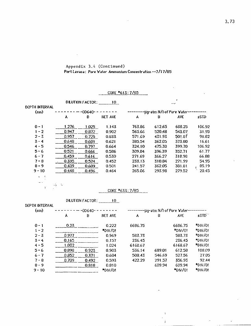
3.73

Appendix 3.4 (Continued) Port l~v~e~: Por(> \y'~t(>r Ammonium Cone(>ntr~tion --7/17/85

DILUTION fACTOR: __ .. __ .. _..1.Q ..•• DEPTH INTERVAL

(em) - - - - - - - - -00640- - - - - - - - ---------~lg-atm NIl of Pore W'ater----------A B NET AVE A B AVE ±STD

0-1 __ t?lL _._1.:Q?;5. .... 1.143 763.86 612.65 688.25 106.92 1 -2 ___ 9.:21L _._ ... _Q.J!?6 .... 0.902 565.66 520.48 543.07 31.95 2-3 ____ .Q.,~.;>.:L _ ....... 9,16;5. .... 0.833 571.69 431.93 ::;01.81 98.82 3-4 _. ___ Q.,§1§ .. ___ .J~)?.Q2 .... 0.621 385.54 362.05 373.80 16.61 4-5 __ .Q";?4L _...!J.:JJ.L 0.664 324.10 475.30 399.70 106.92 5-6 __ O-,§£!... __ QJ?J?:L 0.586 309.04 396.39 352.71 61.77 6-7 _.9-,1;?L ___ 9-,HL 0.530 271.69 366.27 318.98 66.88 7-8 __ Q."~~:? ___ 0-,;?1i... 0.452 233.13 310.84 271.99 54.95 8-9 __ Q"1Q~L ___ .. 9.'§Q~L 0.501 241.57 362.05 301.81 I 85.19 9- 10 _. __ 9,11§_ ._ ... ..,.QA~§ .. _ 0.464 265.06 293.98 279.52 20.45 . ,

D IlUT ION fACTOR: ....... _ ....... ..1.Q •..• DEPTH INTERVAL

(em) - - - - - - - - -OD640- - - - - - - - ---------l1g-atm NIl of Pore \(ater----------A B NET AVE A B AVE iSm"

o - 1 _. ____ Q.,?.~ .... ___ ._ .... ___ ._. 0.222 6E.8b.75 6686.75 IIDIV to!

1 - 2 .. _ ... _ .... __ ........... _ .... _ ..... _._. __ .. _ IIDIV 10! IIDIV/O! IIDIV /O! 2 - 3 ___ ... .Q}}11 .... _ ...... ___ .. _ .. _ 0.969 583.73 583.73 IIDIV/O!

3 - 4 _ ... _ ... .9.J.§;?._ .............. _........... 0.1 57 236.45 236.45 "DIV/O! 4 - 5 _._._LQ;?L _ ..... _._ .... __ ...... 1 .024 6168.67 6168.67 IIDIV /O! 5 - 6 ___ 9.,§~JL _._ ... .Q.,n:L 0.903 536.14 689.01 612.58 108.09 6 - 7 . ____ 9.J~§L __ ...!J"EL.. 0.604 508.43 546.69 527.56 27.05

7 - 8 .... __ Q.,IQ2._. _._ .. 9."126.... 0.593 422.29 291.57 356.93 92.44 8 - 9 ___ ._. ____ .9j:!.!.?_._ 0.810 609.94 609.94 IIDIV/O! 9-10 IIDIV/o! IIDIV lo! IIDIV/O!

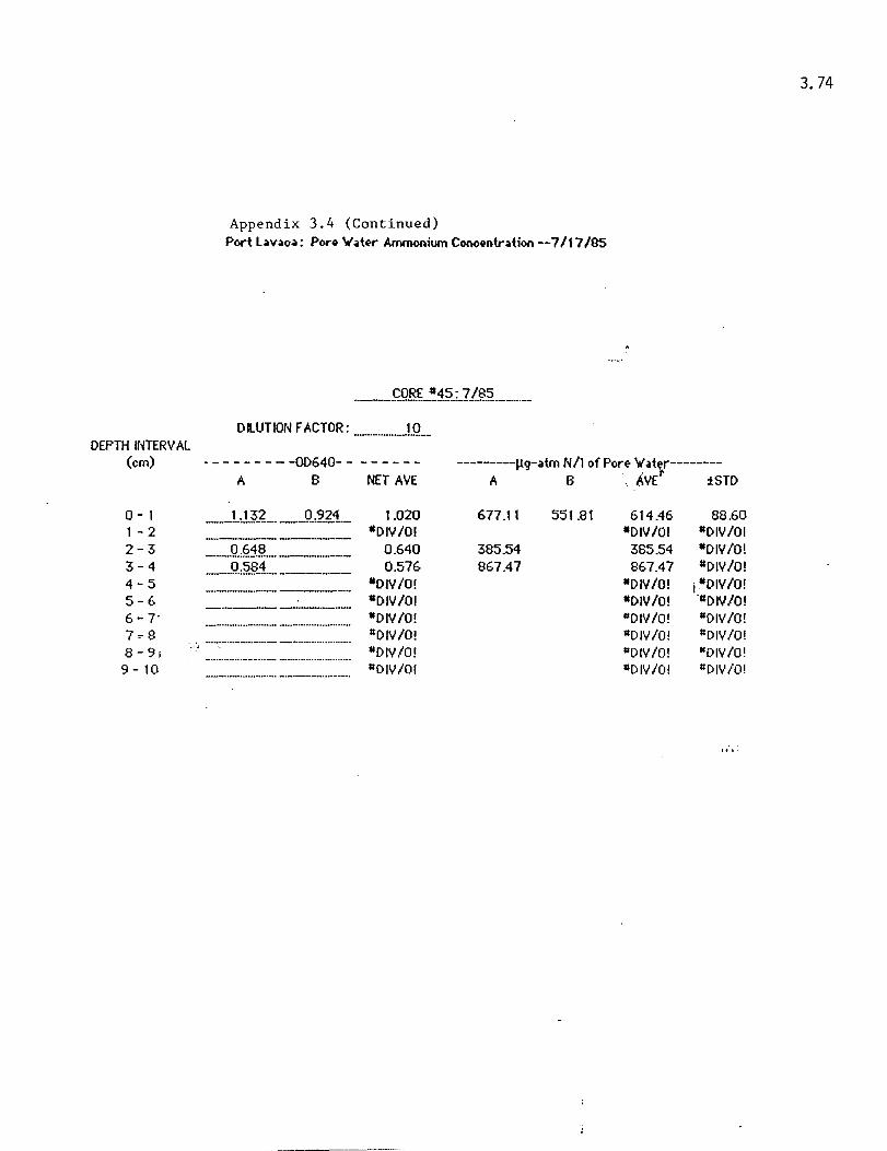
DEPTH INTERVAL (em)

0-1 1 - 2 2-3 3-4 4-5 5-6 6-7' 7~8

8- 91 9 - 10

.. ,

Appendix 3.4 (Continued) Port l .. no .. : Por~ W .. tE'r Ammonium CoooE'ntr .. tion --7/17/BS

DILUTION FACTOR: ___ ......... _.!.Q_

. - - - - - - - -00640- - - - - - - -A B

-------__ 0)~1lL. __ .. __ _ __ Q.:~J?.L ___ . __ _

_._ .•...•••..... --.- -_ .. _ ............. _ .

NET AVE

1.020 11011//01

0.640 0.576

IIDIVIOl 11011//01 IIDIV/O! IIDII//O! IIDIV/O! 1/011//01

---------Ilq-alm 1'111 of Port' Wal~r--------A B- AVE

t iSTD

677.11 551.81 614.46 88.60 IIDIV 101 IIDIV/ol

385.54 385.54 IIDIV lo! 867.47 867.47 IIDIV/o!

IIDIV/O! i IIDIV/O! IIDII//O! ·IIDII//O! IIDIV/O! IIDIV/Ol IIDIV/O! "0 IV 10! IIDIV/O! IIDIV/O! #DII//O! "DIV lor

3.74

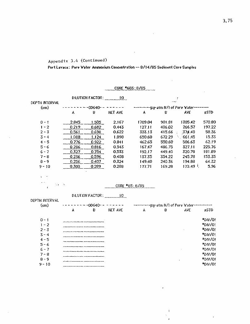
Appendix 3.4 (Continued)

Port l~vaca: PorI! "w'~tl!r Ammonium Concl!ntration -- 8/14/85 SE.'diml!nt Corl! SamplE.'s

DILUTION fACTOR: .. __ .. _ .. _...!.!;L DEPTH INTERVAL

(em) - - - - - - - - -OD640- - - - - - - - ---------Ilg-atm N/l of PorE.' 'ti'atE.'r--------A B NET AVE A B AVE iSm

0- I _ .. _X?1.;? _ __ 1 .50;?_ 2.167 1709.04 901.81 1305.42 570.80 1-2 ___ ...Q.:£.!.L __ Q:§??_ 0.443 127.11 406.02 266.57 19722 2-3 __ 0";?§L_Q.&2!~L 0.622 33;>";.13 415.66 ;37~.40 58.?;6 3-4 __ .LQ?L . __ . .1.:.1.£1 .... 1.098 650.60 672.29 .661.45 15.33 4-5 ..... JQ}L~.?L 0.B41 462.65 550.60 506.63 62.19 5-6 . ____ Q2?L ___ Q.:?.LL 0.543 167.47 486.75 327.11 225.76 6-7 __ Q.}~L _Q:154 _ 0.533 192.17 449.40 320.78 181 .89 7-8 __ .Q:£;?L _....9..:~2§L_ 0.408 137.35 354.22 245.78 153.35 8-9 _Q"2;?'L __ 0~19.L 0.324 149.40 240.36 194.88 64.;>";2

9 -10 _ .. _Q.}Q,L _Jl..:£?L 0.288 177.71 169.28 173.49 i 5.96

.' ~ .'~ ......... _ ... r;.QB.~_~?;?; .. ?.f..W~ ............. .

DEPTH INTERVAL (em)

0-1 1 - 2 2-3 3-4 4-5 5-6 6-7 7-8 8-9

9 - 10

D lLUT ION fACTOR: ................. ..!.Q ... .

- - - - - - - - -OD640- - - - - - - -A B NET AVE

---------~lg-atm N/I of Pore Vater----------A B AVE ±.STD

#DIVIO! #DIV/O! #DIV/O! "DIV/O! "DIV /O! "DIV/O! #DIVIO! "DIV/O! #DIVIO! "DIV/O!

3.75

3.76

Appendix 3.4 (Continued)

Port l~v~c~: Por<~ W'~t~r Ammonium Cono~ntntion -- B/14/85 ~di~nt Con S~mpl~~

DILUTION fACTOR: ................... .1.Q ... . DEPTH INTERVAL

(em) - - - - - - - - -00640" - - - - - - - ---------Ilg-atm NIl of PorE; Water----------A B NET AVE A B AVE ±STD

0-1 .. _ .. Jt1L_ .. Q:1..9.L 0.291 290.36 60.24 175.30 162.72 1 - 2 . ___ .J!::!?L 0.476 286.75 286.75 #DIVIO! 2-3 ... _0.3 .. QL __ .. Q.:.42lL 0.358 178.31 253.01 215.66 52.82 3-4 _ ... _(L?J.:L. __ OJ.~ .. !?' .... 0.198 125.90 112.65 ,11'9.28 9.37 4-5 ... _OJl~'L _ .. ..Q:?1..L 0.196 48.80 187.35 118.D7 97.97 5-6 O.O:p _°-1.?L 0.067 11.45 69.28 40.36 40.89 6-7 .. ______ 0:9..? .. L 0.065 39.16 39.16 #DIV/O! 7-8 __ Q"03 .. L . __ !LQ§L 0.042 14.46 35.54 25.00 14.91 B-9 __ O.O .. ~L_O..:.Q§L 0.037 9.04 34.94 21.99 lB.32 9- 10 __ 0"05L __ .. QR?;? ..... 0.039 30.12 16.27 23.19 i 9.80

, ,

'.:. ,'. ............. ~QRf.: ... ~.§.~}.; .. ?l?:? ............ .

D lLUT ION fACTOR: .................... !.Q ... . DEPTH INTERVAL

(em) - - .. - - - - - -00640" - - - - - - - ---------1l9-~tm NIl of Pore Water--"-"-"---A B NET AVE A B AVE ±STD

0-1 .... _...9..}?!._ .. _L:D:? .... 1.006 448.19 763.25 605.72 222.78 1 - 2 ............ Q.::??? .............. Q.::!??-. 0.530 349.40 289.16 319.28 42.60 2-3 _ .... _.Q.:;?:?I ... _ ...... !U..!.L 0.329 330.72 65.06 197.89 187.85 3-4 .. __ Q"Q;?!? .... ___ Q.P!?L .. 0.054 28.92 35.54 32.23 4.69 4-5 .. __ . ..9}) .. L __ .9"??L 0.938 543.37 5B6.75 565.06 30.67 5-6 ... _Q.:9J"? ___ O"QIL 0.049 17.47 40.96 29.22 16.61 6-7 __ Q"9JJ. __ .. _Q"Q?L 0.036 13.86 29.52 21.69 11.08 7-8 __ Q.:.Q.LL_L;?'?L 0.797 3.01 956.63 479.82 674.31 B-9 _ O.O~L_Q:.L~;L. 0.102 54.22 68.67 61.45 10.22 9- 10 .... _....9.:9)~;?_ .. __ Q.:Q6.L 0.020 16.27 7.83 12.05 5.96

3.77

Appendix 3.4 (Continued) Port lavaca: Pore 'w'att>r Ammonium Conct>ntntion -- 8/14/85 St>dimt>nt Cort> Samplt>s

DILUTION FACTOR: __ ... _J.L DEPTH INTERVAl

(cm) - - - - - - - - -00640- - - - - - - - ---------Ilg-atm 1'1/1 of Pore Water----------A B NET AVE A B AVE ±STD

0-1 __ J:~t67 __ 1~2tL 1.333 878.92 726.51 802.71 107.77 1 - 2 __ LI;!?L.. __ ._Q .. 6fJ?_ 1.221 1098.19 372.29 735.24 51329 2-3 __ 9.A1.L __ .!1!}1._ 0265 281.96 37.35 :l5';l.6~ 172.94 3-4 ____ 9..:~!?L ___ J:))~;?]_ 0.496 206.63 390.96 298.80 130.35 4-5 __ O..:~QL __ qJ:!.LL 0.800 479.52 484.34 481.93 3.41 5-6 ___ O·E?';?_L _9.&_~_ 0.636 390.36 375.30 382.83 10.65 6-7 __ 0.:.I~_1 __ O..:?§L 0.632 429.52 331.33 380.42 69.43 7-8 ___ .Q~;?'],J: .... __ Q.:!?.1_1L 0.605 342.77 385.54 364.16 30.24 8-9 __ !H!lL 0.606 365.06 365.06 !lDIV lot

9 - 10 __ 0.95L_Q:1~L 0.712 568.67 288.55 428.61 i,198.08

, ,

',. ~ :.;

DILUTION FACTOR: __ . .J.Q .... DEPTH INTERVAL

(em) - - - - - - - - -OD640- - - - - - - - ---------Ilg-atm Nil of Pore ylater-----------A B NET AVE A B AVE ±SlJ>,.

0- 1 ___ fJHL ___ ._f.:?:tL 2.839 1709.04 1710.84 1709.94 1.28 1 -2 .... _ .. _-_ ..... -...... -... -.... -~.:~-!? .. - 2.842 1712.05 1712.05 "DIV/O! 2-3 __ . ____ ._ ......... _ .. ___ f.:§!;?.L_ 2.843 1712.65 1712.65 IIDIV lot 3-4 ._ ..... _J.::?;?;L _ .. _ .. _f..:Q.1.:L.. 1.627 750.00 121024 980.12 325.44 4-5 ._ ..... _ .. _Q.:Q.L ._._L?lL 0.935 1.20 1125.30 563.25 794.86 5-6 ___ . __ 9.:?II ... _ ... __ .Q.,tnL 0.879 523.49 535.54 529.52 8.52 6-7 _._._ ..... Q3':?_ .... _ .. _______ ._ 0.712 428.92 428.92 !lDIV lOt 7-8 _._ ........ Q.:2L ____ Q.:;??L!?_ 0.715 543.37 317.47 430.42 159.74 8-9 ___ ._Q.:~?_L __ . .Q.:~Q;L 0.634 586.75 177.11 381.93 289.66 9- 10 "DN/O! "DIV/O! "DIV/O! -..... _-_._._--- _. __ .......... -.. -

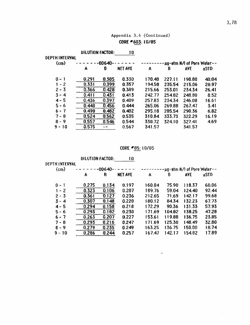
DEPTH INTERVAL

Appendix 3.4 (Continued)

CORE -603: 10/65

DILUTION fACTOR: 10 -----(em) . - - - - --00640-· - - - - - ---------JlQ-atmNllofPoreWater--

A B NET AVE A B AVE :t:STO

0- 1 0.291 0.365 0.330 170.48 227.11 198.80 40.04 1 - 2 0.331 0.399 0.357 194.58 235.54 215.06 28.97 2 - 3 0.366 0.428 0.389 215.66 253.01 234.34 26.41 -' 3-4 0.411 0.431 0.413 242.77 254.82 248.80 8.52 4-5 0.436 0.397 0.409 257.83 234.34 246.08 16.61 5-6 - 0.448--iI456 0.444 265.06 269.88 267.47 3.41 6 - 7 0.498 0.482 0.482 295.18 285.54 290.36 6.82 7-8 0.524 0.562 0.535 310.84 333.73 322.29 16.19 8-9 0.557 0.546 0.544 330.72 324.10 327.41 4.69 ---_. __ .. -9 - 10 0.575 0.567 341.57 341.57 -------------_.-

CORE -85: 10/85

DILUTION fACTOR: 10 _._ .. _-_. DfPTHINTfRVAl

(em) . - - - - - -00640- . - - - - - - - - - - - - - - llg-atm Nil of Pore Water--A B NET AVE A B AVE :t:STD

0- 1 0.275 0.134 0.197 160.84 75.90 118.37 60.06 ---_ .. __ .... _-_ .. _-1 - 2 0.323 0.106 0.207 189.76 59.04 124.40 92.44 2 - 3 0.361 0.127 0.236 212.65 71.69 142.17 99.68 3-4 0.307 0.146 0.220 180.12 84.34 132.23 67.73 4- 5 0.294 0.158 0.218 172.29 90.36 131.33 57.93 5-6 0.293 0.182 0.230 171.69 104.82 138.25 47.28 6-7 0.263 0.207 0.227 153.61 119.88 136.75 23.85 7-8 0.293 0.216 0.247 171.69 125.30 148.49 32.80 8-9 0.279 0.235 0.249 163.25 136.75 150.00 18.74 9 - 10 -0.286 0.244 0.257 167.47 142.17 154.82 17.89

3.78

)EPTH INTERVAL

Appendix 3.4 (Continued)

CORE -65: 10/85

DILUTION fACTOR: 10 -----(em) • - - - - --00640-· - - - - - ---------Jlg-atm Nil ofPoreWater--

A B NET AVE A B AVE iSTD

0- 1 0.272 0.269 0.263 159.04 157.23 158.13 1.28 1 - 2 0.245 0.297 0.263 142.77 174.10 158.43 22.15 -------_ .. _-2 - 3 0.244 0.279 0.254 142.17 163.25 152.71 14.91 3 - 4 0.245 0.186 0.208 142.77 176.75 160.76 25.44 4-5 0.223 0.218 0.213 129.52 126.51 128.01 2.13 5-6 0.163 0.139 0.143 1.52 78.9£ 40.22 54.73 6-7 0.036 0.028 168.67 168.67 7-8 8-9 0.245 0.103 0.166 142.77 143.07 142.92 0.21 9 - 10 0.371 0.155 0.255 218.67 88.55 153.61 92.01

CORE -623: 10/85

DILUTION fACTOR: 10 lEPTH INTERVAL

(em) . - - - - - -00640-· - - - - - - - - - - - - - - Jlg-8tm Nil of Pore Water--A 8 NET AVE A B AVE :t:STD

0- I 0.239 0.328 0.276 139.16 192.77 165.96 37.91 I - 2 0.184 0.202 0.185 106.02 116.87 111.45 7.67 2-3 0.236 0.294 0.257 137.35 172.29 154.62 24.71 _._-_ ...... 3 - 4 0.305 0.337 0.313 178.92 198.19 188.55 13.63 4-5 0.361 0.433 0.389 212.65 256.02 234.34 30.67 5-6 0.419 0.478 0.441 247.59 283.13 265.36 25.13 6-7 ---0~5-··b.48r 0.483 296.39 284.94 290.66 8.09 7 - 8 0.519 0.496 0.500 307.83 293.98 300.90 9.80 8-9 0.478 0.5 0.481 283.13 296.39 289.76 9.37 9 - 10 0.509 0.473 0.483 301.81 280.12 290.96 15.33

3.79

3.80

Appendix 3.4 (Continued)

CORE -613: 10/85

DILUTION fACTOR: 10 )EPTH INTERVAL

(em) • - - - - - -00640-· - - - - - - - - - - - - - - J,lq-etm Nil of Pore Weter--A B NET AVE A B AVE :l:5TD

0- I 0.219 0.237 0.220 127.11 137.95 132.53 7.67 1 - 2 0.277 0.311 0.286 162.05 182.53 172.29 14.48 2-3 0.326 0.337 0.324 191.57 198.19 194.88 4.69 3-4 0.399 0.365 0.374 235.54 215.06 225.30 14.48 4-5 0.401 0.436 0.411 236.75 257.83 247.29 14.91 5-6 0.433 0.481 0.449 256.02 284.94 270.48 20.45 6 - 7 0.466 0.478 0.464 275.90 283.13 279.52 5.11 7 - 8 0.43 0.488 0.451 254.22 289.16 271.69 24.71 8-9 0.437 0.477 0.449 258.43 282.53 270.48 17.04 9 - 10 0.44 0.493 0.459 260.24 292.17 276.20 22.58 ---------

CORE "'633: 10/85

DILUTION fACTOR: 10 ---__ ... _0-lEPTH INTERVAL

(em) . - - - - - -OD64O-· - - - - - - - - - - - - - -J.lg-etm Nil of Pore Weter--A B NET AVE A B AVE :l:STD

0- 1 0.7130.661 0.679 424.70 393.37 409.04 22.15 1 - 2 -·-----1fT62 0.154 463.86 463.86 -----_._-_. 2-3 0.102 0.094 283.13 283.13 3-4 0.076 0.068 409.64 409.64 4- 5 5-6 6-7 7-8 8-9 0.488 0.522 0.497 289.16 309.64 299.40 14.48 -------9 - 10 0.579 0.525 0.544 343.98 311.45 327.71 23.00

Appendix 3.4 (Continued)

CORE -603: 1214165

DILUTION fACTOR: 10 DEPTH INTERVAL

(em) . - - - - - -OD64O-· - - - - - - - - - - ----Jlg-atm Nil of Pore Water--A B NET AVE A B AVE :tSTD

0- 1 ___ 9.:.!!66 _ 0.074 0.065 37.35 36.55 37.95 0.65 1 - 2 0.077 0.105 0.083 42.77 57.23 50.00 10.22 -----------2 - 3 0.143 0.158 0.143 82.53 89.16 65.84 4.69 3-4 0.198 0.229 0.206 115.66 131.93 123.80 11.50 4-5 0.291 0.261 0.268 171.69 151.20 161.45 14.46 5-6 -·--0.363- 0.267 0.307 215.06 154.82 184.94 42.60 6-7 0.393 0.326 0.352 233.13 190.36 211.75 30.24 7-8 0.445 --0.337 0.383 264.46 196.99 230.72 47.71 8-9 0.524 0.346 0.428 312.05 203.61 257.83 76.67 9 - 10 0.5 0.356 0.420 297.59 208.43 253.01 63.04 _ ..... _-

CORE -85: 12/4/85

DILUTION fACTOR: 10 _._--DEPTH INTERVAL

(em) . - - - - - -00640-· - - - - - ---------Jlg-atm Nil of Pore Water--A B NET AVE A B AVE :f:STD

0- 1 0.208 0.124 0.156 119.28 68.67 93.98 35.78 1 - 2 -013"60.156 0.137 75.90 89.16 62.53 9.37 2 - 3 0.123 0.129 0.116 68.07 71.69 69.88 2.56 3-4 0.107 0.151 0.119 58.43 84.94 71.69 18.74 -----4-5 0.101 0.167 0.124 54.82 94.56 74.70 28.11 5-6 0.1 0.17 0.125 54.22 96.39 75.30 29.62 6-7 0.116 0.22 0.159 65.06 126.51 95.78 43.45 7-6 __ .....9..112 0.236 0.164 61.45 136.14 98.80 52.82 8-9 0.117 0.294 0.196 64.46 171.08 117.77 75.40 9 - 10 0.129 O~32 0.215 71.69 186.75 129.22 81.36 --_.-

3.81

Appendix 3.4 (Continued)

CORE -65: 12/4/85

DILUTION fACTOR: 10 IEPTH INTERVAL

(em) . - - - - - -00640-· - - - - - ---------JlC,l-atm Nil of Pore Water--A B NET AVE A B AVE ~STD

0- 1 0.093 0.154 0.116 50.00 69.16 69.56 27.69 1 - 2 0.078 0.084 0.073 40.96 46.99 43.98 4.26 2-3 0.093 0.108 0.093 50.00 61.45 55.72 8.09 3-4 0.068 0.068 0.060 34.94 37.35 36.14 1.70 4-5 0.073 0.057 0.057 37.95 30.72 34.34 5.11 5-6 0.083 0.069 0.068 43.96 37.95 40.96 4.26 6-7 0.085 0.066 0.066 45.18 36.14 40.66 6.39 -----7-8 0.091 0.064 0.070 48.80 34.94 41.87 9.80 8 - 9 0.095 0.068 0.074 51.20 37.35 44.28 9.80 ------

9 - 10 0.093 0.08 0.079 50.00 44.58 47.29 3.83 ----

CORE -623: 1214185

DILUTION FACTOR: 10 ----IEPTH INTERVAL

(em) . - - - - --00640-· - - - - - ---------Jlg-atmNil of PoreW8ter--

0- 1 1 - 2 2-3 3-4 4-5 5-6 6-7 7-8 8-9 9 - 10

A B NET AVE A B AVE ±STO

0.149 0.09 _._----_ .. _---_ .. -0.132 0.114 _ .. _ .... _. __ . 0.166 0.182 --_._-_ ....... _-_ .. _-0.224 0.226 -_ .. _------0.334 0.258 --------_.

0.24 0.291 0.285 0.277

0.29 0.306 0.336 0.334 0.332 0.355

0.115 0.118 0.169 0.220 0.291 0.261 0.276 0.293 0.330 0.339

86.75 76.51 96.99

131.93 198.19 141.57 168.67 171.69 199.40 196.99

50.60 65.06

106.02 132.53 151.81 171.69 163.25 180.72 197.59 210.24

68.67 70.78

101.51 132.23 175.00 156.63 165.96 176.20 198.49 203.61

25.56 8.09 6.39 0.43

32.80 21.30

3.83 6.39 1.28 9.37

3.82

----- - ------- ------

3.83

Appendix 3.4 (Continued)

CORE -45: 12/4/85

DILUTION fACTOR: . __ -1~_ DEPTH INTERVAL

(em) • - - - - - -OD640-· - - - - - - - - - - ----llC]-atm Nil of Pore Water--A B NET AVE A B AVE ±STD

0- 1 0.076 0.127 0.092 39.76 70.48 55.1 Z 21.72 1 - 2 0.134 0.093 0.104 74.70 83.35 79.02 6.12 2-3 0.042 0.187 0.105 96.39 106.63 101.51 7.24 3-4 0.168 0.256 0.202 95.18 148.19 121.69 37.49 ---4-5 0.185 0.26 0.213 105.42 150.60 128.01 31.95 5-6 0.208 0.233 0.211 119.28 134.34 126.81 10.65 6-7 0.152 0.215 0.174 85.54 123.49 104.52 26.84 7 - 8 0.153 0.203 0.168 86.14 116.27 101.20 21.30 8-9 0.128 0.168 0.138 71.08 95.18 83.13 17.04

9 - 10 0.132 0.156 0.134 73.49 87.95 80.72 10.22 _ .. _. __ 0_. ___ 0_-

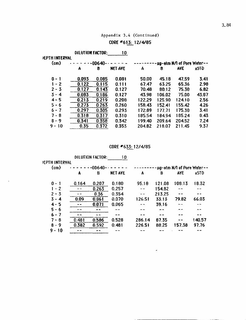
)EPTH INTERVAL

Appendix 3.4 (Continued)

CORE -613: 1214/65

DILUTION fACTOR: 10

(em) . - - - - - -00640-· - - - - - ------ ---nQ-etm Nil of Pore Water--A B NET AVE A B AVE :tSTD

0- 1 0.093 0.065 0.081 50.00 45.16 47.59 3.41 1 - 2 0.122 0.115 0.111 67.47 63.25 65.36 2.96 2-3 0.127 0.143 0.127 70.46 60.12 75.30 6.62 3-4 0.063 0.166 0.127 43.96 106.02 75.00 43.67 4-5 0.213 0.219 0.208 122.29 125.90 124.10 2.56 5-6 -0273-0.263 0.260 158.43 152.41 155.42 4.26 -------6-7 0.297 0.305 0.293 172.89 177.71 175.30 3.41 7-8 0.318 0.317 0.310 185.54 184.94 185.24 0.43 6-9 _~~_1_0.358 0.342 199.40 209.64 204.52 7.24

9 - 10 0.35 0.372 0.353 204.82 218.07 211.45 9.37 ---_ ... _-_ .. _--

CORE -633: 1214/85

DILUTION FACTOR: 10 lEPTH INTERVAL

(em) - - - - - --00640-· - - - - - ---------ng-etmNllofPoreWeter--A B NET AVE A B AVE :l:5TO

0- 1 0.164 0.207 0.180 95.18 121.08 108.13 18.32 .. _-_ ... _----_._--1 - 2 0.263 0.257 154.82 2-3 0.36 0.354 213.25 3-4 --O~O9-O:~ 0.070 126.51 33.13 79.82 66.03 4-5 0.071 0.065 39.16 5-6 6-7 7 - 8 0.461 0.586 0.528 286.14 87.35 140.57 8-9 0.382 0.592 0.481 226.51 88.25 157.38 97.76 9 - 10

3.84

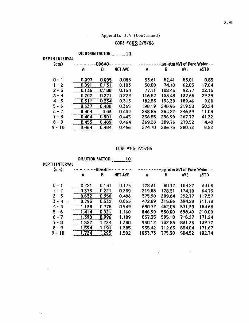
3.85

Appendix 3.4 (Continued)

CORE #603: 215/66

DILUTION fACTOR: 10 DEPTH INTERVAL

(em) . - - - - - -00640-· - - - - - -------- -J19-atm Nil of Pore Water--A B NET AVE A B AVE iSm

0- 1 0.097 0.095 0.088 53.61 52.41 53.01 0.85 1 - 2 0.091 0.131 0.103 50.00 74.10 62.05 17.04 2-3 0.136 0.168 0.154 77.11 108.43 92.77 22.15 3-4 0.202 0.271 0.229 116.67 158.43 137.65 29.39 4-5 0.311 0.334 0.315 182.53 196.39 189.46 9.80 5-6 _0.337 __ 0.40ft 0.365 198.19 240.96 219.58 30.24 6-7 0.404 0.43 0.409 238.55 254.22 246.39 11.08 7-8 0.404 0.501 0.445 238.55 296.99 267.77 41.32 8-9 0.455 0.489 0.464 269.28 289.76 279.52 14.48 9 - 10 0.464 0.464 0.466 274.70 286.75 280.72 8.52 --_._-_._-_.-

CORE #85: 215/86

DILUTION FACTOR: 10 ---_ .. _-. DEPTH INTERVAL

(em) . - - - - - -00640- . - - - - - - - - -- - - - -J1g-etm Nil of Pore Water--It B NET AVE A B AVE i5TO

0- 1 0.221 0.141 0.173 128.31 80.12 104.22 34.08 1 - 2 0.373 O~22T 0.289 219.88 128.31 174.10 64.75 2-3 0.632 0.356 0.486 375.90 209.64 292.77 117.57 3-4 0.793 0.532 0.655 472.89 315.66 394.28 111.1 B 4-5 1.136 0.775 0.949 680.72 462.05 571.39 154.63 5-6 1.414 0.921 1.160 846.99 550.00 698.49 210.00 6-7 1.398 0.996 1.189 837.35 595.18 716.27 171.24 7-8 1.552 1.224 1.380 930.12 732.53 831.33 139.72 8 - 9 1.594 1.191 1.385 955.42 712.65 834.04 171.67 9 - 10 1.724 1.295 1.502 1033.73 775.30 904.52 182.74

IEPTH INTERVAL

Appendix 3.4 (Continued)

CORE -65: 215/86

DILUTION fACTOR: ___ ... _.!..Q_

(em) - - - - - --00640-- - - - - - ---------llg-atmNil of Pore Water--A B NET AVE A B AVE :tSTO

0- 1 0.135 0.08 0.100 76.51 72.30 74.40 2.97 1 - 2 0.08 0.178 0.121 43.37 102.41 72.89 41.74 2-3 - .. 0.126·- 0.157 0.134 71.08 89.76 80.42 13.21 3-4 0.159 0.245 0.194 90.96 142.77 116.87 36.63 ----------4-5 0.1390.241 0.182 78.92 140.36 109.64 43.45 5-6 0.123 0.265 0.186 69.28 154.82 112.05 60.49 6-7 0.126 0.2 0.155 71.08 115.66 93.37 31.52 7 - 8 0.131 0.171 0.143 74.10 98.19 86.14 17.04 6 - 9 0.163 0.144 0.146 93.37 81.93 87.65 8.09

9 - 10 0.176 0.148 0.154 101.20 84.34 92.77 11.93 -_._-..... _---

CORE -623: 2/5/86

DILUTION FACTOR: 10 ------IEPTH INTERVAL

(em) - - - - - - -00640-· - - - - - - - - - - - - - - Jig-etm Nil of Pore Weter--A B NET AVE A B AVE :tSTO

0- 1 0.103 0.098 0.093 57.23 54.22 55.72 2.13 1 - 2 ---O:08s--oT37 0.105 48.19 77.71 62.95 20.67 2-3 0.112 0.149 0.123 62.65 84.94 73.80 15.76 -------3-4 0.126 0.187 0.149 71.06 107.83 89.46 25.98 4-5 0.147 0.176 0.154 63.73 101.20 92.47 12.35 5-6 0.162 0.189 0.168 92.77 109.04 100.90 11.50 6-7 0.178 0.178 0.170 102.41 102.41 102.41 0.00 7-8 0.175 0.196 0.178 100.60 113.25 106.93 8.95 --_ .. _-----6-9 0.184 0.206 0.187 106.02 119.28 112.65 9.37 9 - 10 0.178 0.212 0.187 102.41 122.89 112.65 14.48

3.86

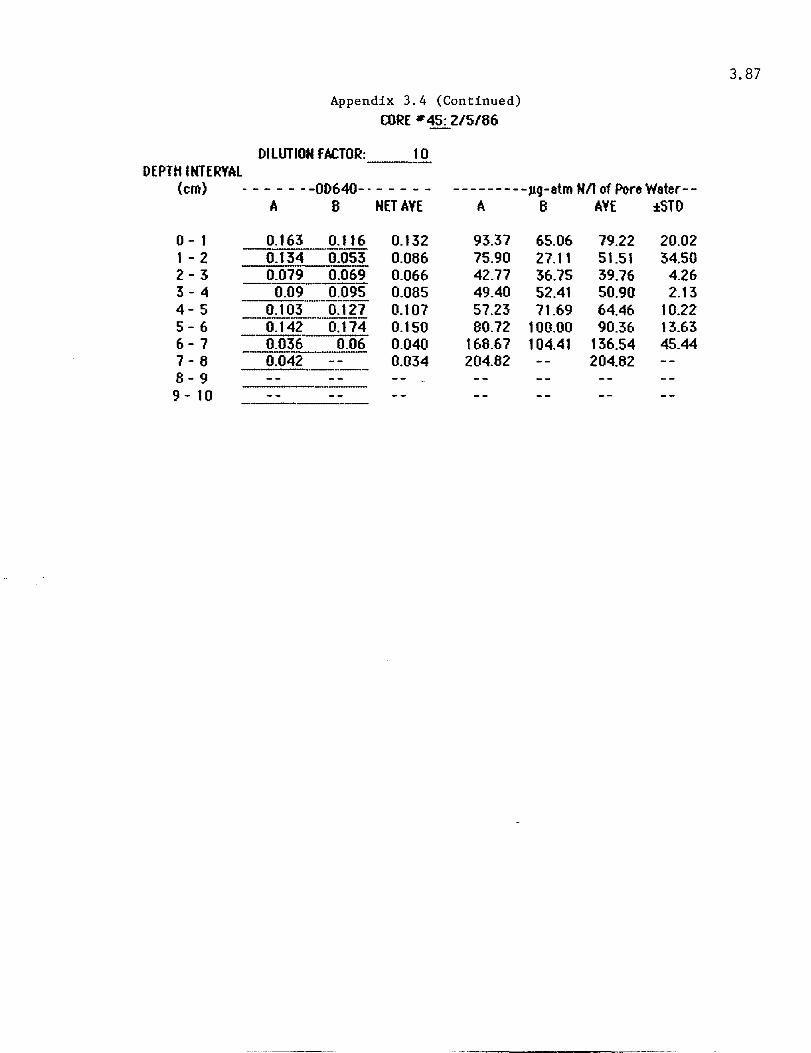
OEPTHINTfRVAl

Appendix 3.4 (Continued)

CORE II 45: 215/66

DILUTION fACTOR: 10 ---"-(em) - - - - - --00640-· - - - - - ---------JIg-etmNil of PoreWeter--

A B NET AVE A B AVE :l:STO

0- 1 0.163 0.116 0.132 93.37 65.06 79.22 20.02 1 - 2 0.134 0.053 0.066 75.90 27.11 51.51 34.50 2-3 0.079 0.069 0.066 42.77 36.75 39.76 4.26 ------3 - 4 0.09 0.095 0.085 49.40 52.41 50.90 2.13 ----------4-5 0.103 0.127 0.107 57.23 71.69 64.46 10.22 -----.----5-6 0.142 0.174 0.150 80.72 100.00 90.36 13.63 6-7 0.036-- 0.06 0.040 168.67 104.41 136.54 45.44 7-6 0.042 0.034 204.82 204.82 8-9 9 - 10

3.87

3.88

Appendix 3.4 (Continued)

CORE -613: 2/5/86

DILUTION fACTOR: 10 IEPTH INTERVAL

(em) - - - - - - -00640- - - - - - - -- -------ng-atm Nil of Pore Water--A 8 NET AVE A 8 AVE tSTO

0- 1 0.062 0.057 0.052 32.53 29.52 31.02 2.13 1 - 2 0.056 0.081 0.061 26.92 43.96 36.45 10.65 2-3 0.082 0.113 0.090 44.56 63.25 53.92 13.21 3-4 0.11 0.15 0.122 61.45 65.54 73.49 17.04 4-5 0.153 0.163 0.160 87.35 105.42 96.39 12.78 5 - 6 0.186 0.227 0.199 107.23 131.93 119.58 17.46 6-7 0.224 0.261 0.245 130.12 164.46 147.29 24.26 7-8 0.238 --0.321 0.272 138.55 188.55 163.55 35.36 8-9 0.26 0.354 0.309 163.66 206.43 . 166.14 31.52 9 - 10 0.274 0.367 0.323 160.24 226.31 194.26 48.13 -_._-_._ ..... _---

CORE #633: 215/66

DILUTION FACTOR: 10 -------IEPTH INTERVAL

(em) . - - - - - -00640-' - - - - - ---------Jlg-atm Nil of PoreWoter--A B Nfl AVE A B AVE ±STO

0-1 0.26 0.172 0.208 151.81 98.80 125.30 37.49 1 - 2 ~~~ l[i~5'-- 0.2i!.. 0.260 166.87 146.39 156.63 14.48 2 - 3 0.351 0.292 0.314 206.63 171.06 168.66 25.13 3-4 0.539 0.367 0.445 319.88 216.27 268.07 73.27 4-5 0.623 0.471 0.539 370.46 278.92 324.70 64.75 5-6 0.753 0.574 0.656 448.60 340.96 394.86 76.25 6-7 0.848 0.708 0.770 506.02 421.69 463.86 59.64 7-8 0.854 0.832 0.635 509.64 496.39 503.01 9.37 6 - 9 0.654 0.818 0.828 509.64 487.95 498.80 15.33 9 - 10 0.885 1.097 0.983 528.31 656.02 592.17 90.31

3.89

Appendix 3.4 (Continued)

CORE -603: 4/9/86

DILUTION fACTOR: 10 ---DEPTH INTERVAL

(em) - - - - - - -00640-· - - - - - - - - - - - - - -llg-atm Nil of Pore Water--A B NET AVE A B AVE :l:STD

0- 1 0.114 0.347 0.226 65.66 205.42 135.54 98.82 1 - 2 0.123 0.326 0.220 71.08 192.77 131.93 86.05 2-3 0.186 0.389- 0.283 109.04 230.72 169.88 86.05 3-4 0.232 0.408 0.315 136.75 242.17 189.46 74.54 4-5 0.262 0.423 0.338 154.82 251.20 203.01 68.15 5-6 0.324 0.448 0.381 192.17 266.27 229.22 52.39 6-7 0.388 0.507 0.443 230.72 301.81 266.27 50.26 7 - 8 0.435 0.552 0.489 259.04 328.92 293.98 49.41 8-9 0.495 0.596 0.542 295.18 356.63 325.90 43.45 9 - 10 0.541 0.646 0.589 322.89 385.54 354.22 44.30

CORE -85: 4/9/86

DILUTION FACTOR: 10 _._------DEPTH INTERVAL

(em) . - - - - - -00640- . - - - - - - - - - - - - - -llg-atm Nil of Pore Water--A B NET AVE A B AVE :l:S1O

0- 1 0.204 0.12 0.156 118.07 68.67 93.37 34.93 _ .. _ ...... _ ... _ ... -1 - 2 0.156 0.099 0.122 89.16 56.02 72.59 23.43 ._ ..... _. __ ._-_._-2 - 3 0.072 0.078 0.069 38.55 43.37 40.96 3.41 ---.-------3-4 0.087 0.082 0.079 47.59 45.78 46.69 1.28 ---------4-5 0.093 0.095 0.088 51.20 53.61 52.41 1.70 5-6 0.102 0.109 0.100 56.63 62.05 59.34 3.83 6-7 0.113 0.12 0.111 63.25 68.67 65.96 3.83 7-8 0.13 0.139 0.129 73.49 80.12 76.81 4.69 -----8-9 0.149 0.148 0.143 84.94 85.54 85.24 0.43 9 - 10 0.133 0.172 0.147 75.30 100.00 87.65 17.46

3.90

Appendix 3.4 (Continued)

CORE -65: 4/9/66

DILUTION fACTOR: 10 )EPTH INTERVAL

(em) . - - - - - -00640-· - - - - - - - - - - - - - -J1g-atm Nil of Pore Water--A B NET AVE A B AVE iSm

0- 1 0:117 0.292 0.199 66.67 267.21 177.04 155.80 1 - 2 0.13 0.251 0.165 74.70 246.03 160.37 121.15 ---------2-3 0.159 0.201 0.174 92.17 195.62 144.00 73.29 :5 - 4 0.142 0.142 0.136 61.93 136.57 109.25 36.64 ._---------4-5 O. 125 0.17 0.142 71.69 164.69 " 8.19 65.76 --- -5-6 0.121 0.165 0.137 69.28 159.67 114.47 63.92 6-7 0.141 0.191 0.160 61.33 185.78 133.55 73.86 7-6 -(f.T43'---0:306 . 0.219 62.53 301.27 191.90 154.67 --_._--8-9 0.149 0.197 0.167 86.14 191.81 138.98 74.71 _._---_. __ . 9 - 10 0.146 0.248 0.191 84.34 243.02 163.66 112.21 _ ...... __ . __ ._-------

CORE -623: 4/9/86

OllLlTION FACTOR: 10 - .. --IEPTH INTERVAL

(em) . - - - - - -00640-· - - - - - - - - - - - - - - J1g-atm NIl of Pore Water--A B NET AVE A B AVE :l:STD

0- 1 0.113 0.157 0.130 64.46 91.57 76.01 19.17 1 - 2 0.149 0.188 0.164 86.14 110.24 96.19 17.04 2 - 3 0.142 0.214 0.173 81.93 125.90 103.92 31.10 . __ .. _----_.-3-4 0.139 0.209 0.169 80.12 122.69 101.51 30.24 4-5 0.156 0.169 0.168 90.36 110.64 100.60 14.48 ------_.-... _-_ .. 5-6 0.203 0.186 0.190 118.67 109.04 113.86 6.82 6-7 0.21 0.165 0.193 122.69 106.43 115.66 10.22 7-6 0.22 0.161 0.196 126.92 106.02 117.47 16.19 8-9 0.198 0.194 0.191 115.66 113.86 114.76 1.26 9 - 10 0.221 0.221 0.216 129.52 130.12 129.82 0.43

DEPTHINTERYAL

Appendix 3.4 (Continued)

CORE'" 45: 4/9/66

DILUTION fACTOR: 1 0 -----(em) . - - - - --00640-· - - - - - ---------Jig-atmNil of Pore Water--

A B NET AVE /It B AVE :t:STD

0- 1 0.064 0.238 0.146 35.54 138.55 87.05 72.84 1 - 2 0.058 0.141 0.095 31.93 200.30 116.11 119.06 2-3 0.092 0.305 0.194 52.41 223.64 138.03 121.08 --------3-4 4-5 ----------5-6 ---6 - 7 7-6 ----------8-9 9 - 10 --_.-

3.91

3.92

. Appendix 3.4 (Continued)

CORE - 613: 4/9/86

DILUTION fACTOR: 10 -'--IEPTH INTERVAL (em) • - - - - --00640-' - - - - - ---------llQ-atmNil of PoreWater--

A 8 NET AVE A 8 AVE :l:STD

0- 1 0.096 0.126 0.106 54.82 72.89 63.86 12.78 1 - 2 0.074 0.098 0.081 41.57 56.02 46.80 10.22 2-3 0.056 0.083 0.065 30.72 46.99 38.86 11.50 __ , ___ 0 __ -

3-4 0.054 0.078 0.061 29.52 43.98 36.75 10.22 4-5 0.078 0.089 0.079 43.98 50.60 47.29 4.69 5-6 --o.f03"··-O.1 07 0.100 59.04 61.45 60.24 1.70 6-7 0.136 0.135 O. t 31 78.92 78.31 78.61 0.43 7-8 0.174 0.185 0.175 101.81 108.43 105.12 4.69 8-9 0.247 0.24 0.239 145.78 141.57 143.67 2.98 9 - 10 0.306 0.278 0.287 181.33 164.46 172.89 11.93 ----

CORE -633: 4/9/86

DILUTION FACTOR: 10 --.---IEPTH INTERVAL

(em) . - - - - - -00640-· - - - - - - - - - - - - - - .ug-etm Nil of Pore Water--A B NET AVE A B AVE ±STD

0- 1 0.243 0.27 0.250 143.07 159.04 151.05 11.29 1 - 2 --'0.294 0.358 0.319 173.80 212.05 192.92 27.05 -_._--2 - 3 0.346 0.391 0.362 205.12 231.93 218.52 16.96 3 - 4 0.192 0.376 0.277 280.87 222.89 251.88 41.00 4-5 0.258 0.408 0.326 380.27 242.17 311.22 97.65 5-6 0.738 0.439 0.582 441.27 260.84 351.05 127.58 6-7 ---O.76i 0.512 0.633 458.73 304.82 381.78 108.83 7 - 8 0.869 0.541 0.698 520.18 322.29 421.23 139.93 8-9 0.916 0.587 0.745 546.49 350.00 449.25 140.36 9 - 10 0.982 0.643 0.806 588.25 383.73 485.99 144.62

DEPTH INTERVAL

Appendix 3.4 (Continued)

CORE #603: 6/4/86

DILUTION fACTOR: to

(em) - - - - - --00640-· - - - - - ---------llg-atmNil of PoreWater-----1\ B NET AVE A B I\VE 1oSTO

0-1 65.06 70.48 67.77 3.83 1 - 2 90.96 77.71 84.34 9.37 2-3 89.16 78.92 84.04 7.24 3-4 97.59 66.55 93.07 6.39 4-5 110.84 102.41 106.63 5.96 5-6 128.92 128.31 128.62 0.43 6-7 139.16 143.37 141.21 2.98 7-8 168.00 151.20 159.60 11.88 6-9 180.72 115.30 118.01 3.83

9 - 10 184.94 201.20 193.07 11.50

CORE #85: 6/4/86

DILUTION FACTOR: 10 DEPTH INTERVl\l

(em) - - - - - --OD640-· - - - - - ---------llg-etmNllofPoreWeter-----A B NET AVE flo B AVE 105TD

0- 1 80.72 61.45 71.09 13.63 1 - 2 101.20 62.65 81.93 27.26 2-3 83.13 57.23 10.18 18.31 3 - 4 60.84 48.80 54.82 8.51 4- 5 62.65 50.00 56.33 8.94 5-6 63.86 56.63 60.25 5.11 6-7 71.08 61.45 66.27 6.81 1-8 74.10 68.07 71.09 4.26 8-9 72.89 75.90 74.40 2.13 9 - 10 98.19 74.70 86.45 16.61

3.93

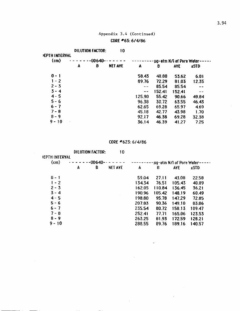
IEPTH INTERVAL

Appendix 3.4 (Continued)

CORE -65: 6/4/86

DILUTION fACTOR: 10

(em) . - - - - - -OD64O-· - - - - - ---------.uQ-etm Nil of PoreWeter----· A B NET AVE A B AVE :tSTO

0- 1 58.43 48.80 53.62 6.81 1 - 2 89.76 72.29 81.03 12.35 2-3 85.54 85.54 3 - 4 152.41 152.41 4-5 125.90 55.42 90.66 49.84 5-6 96.38 30.72 63.55 46.43 6-7 62.65 69.28 65.97 4.69 7-8 45.18 42.77 43.98 1.70 8-9 92.17 46.38 69.28 32.38 9 - 10 36.14 46.39 41.27 7.25

CORE -623: 6/4/86

DILUTION FACTOR: 10 lEPTH INTERVAL

(em) . - - - - --00640-· - - - - - ---------.ug-otm NIl ofPoreWater-----

0- 1 1 - 2 2-3 3-4 4-5 5-6 6-7 7-8 8-9 9 - 10

A B NET AVE A B AVE :l:STO

59.04 134.34 162.05 190.96 198.80 207.83 235.54 252.41 263.25 288.55

27.11 76.51

110.84 105.42 95.78 90.36 80.72 77.71 81_93 89.76

43.08 105.43 136.45 148.19 147.29 149.10 158.13 165.06 172.59 189.16

22.58 40.89 36.21 60.49 72.85 83.06

109.47 123.53 128.21 140.57

3.94

Appendix 3.4 (Continued)

Core #613 - 6/4/86

Depth Interval (em)

0-1

1-2

2 - 3

3 - 4

4 - 5

5 - 6

6 - 7

7 - 8

8 - 9

9 - 10

llg-atm NLI of Pore Water A B AVE

65.66 65.66 65.66

84.34 66.87 75.61

82.53 62.65 72.59

69.88 60.84 65.36

63.86 56.02 59.94

66.86 60.84 63.85

71.08 63.25 67.17

77.71 72.89 75.30

95.18 89.76 92.47

114.46 115.66 115.03

3.95

±STD

0.00

12.35

14.06

6.39

5.54

4.26

5.54

3.41

3.83

0.81

DEPTHINTERYAl

Appendix 3.4 (Continued)

CORE" 45: 6/4/86

DILUTION FACTOR: 1 0

(em) . - - - - --00640-· - - - - - ---------lLg-atmNnofPoreWater--

0- 1 1 - 2 2-3 3-4 4-5 5-6 6-7 7-8 8-9 9 - 10

A B NET AVE A B AVE tSTO

107.23 153.01 168.07

194.58 165.06 193.37 241.57 248.80 266.27 286.14

107.23 153.01 168.07 194.58 165.06 193.37 241.57 248.80 266.27 286.14

3.96

Appendix 3.4 (Continued) Table . Core #633 - 6/4/86

Depth Interval (em)

0-1

1-2

2 - 3

3 - 4

4 - 5

5 - 6

6 - 7

7 - 8

8 - 9

9 - 10

3.97

gg-atm NLJ of Pore Water A B AVE ±STD

124.70 118.07 121.39 4.69

283.13 422.29 352.71 98.40

265.06 521.69 393.38 181.46

168.67 428.31 298.49 183.59

29 l.I 6 554.22 422.69 186.01

227.91 227.91

Appendix 3.4 (Continued)

CORE 11(,()3: 8161&6

!>LUTUf F ACT~: 10 >EPTH INTERVAl..

(em) ------~.----- -----Jlq-atm Nil of Pon ..... atH'---

A B NET AVE A B AVE :tST!>

0-1 78.31 80.12 79.22 1.28 1 - 2 120.48 118.67 119.58 1.28 2-3 136.14 171.08 153.61 24.71 3-4 146.39 196.38 171.39 35.35 4-5 169.28 213.86 191.57 31.52 5-6 177.71 210.84 194.28 23.43 6-7 182.53 215.06 198.80 23.00 7-8 189.76 207.00 198.38 12.19 8-9 194.58 218.07 206.33 16.61 9-10 196.99 230.72 213.86 23.85

CORE ass: B/6/86

DIlUUlH FACTOR: 10 )EPTH IHTERV AI..

(em) - - - - - - -00640- . - - - - - -------Ilg-atm Nil of Pore 'w'ater-----

0-1 1 - 2 2-3 3-4 4-5 5-6 6-7 7-8 8-9 9 - 10

A B NET AVE A

40.36 119.28 165.06 189.76 189.16 127.11 151.20 131.32 116.87 109.04

B AVE :tST!>

74.10 5723 23.86 155.42 137.35 25.55 200.60 182.83 25.13 267.47 228.62 54.95 268.07 228.62 55.80 234.34 180.73 75.82 267.47 209.34 8222 219.88 175.60 62.62 201.20 159.04 59.63 189.76 149.40 57.08

3.98

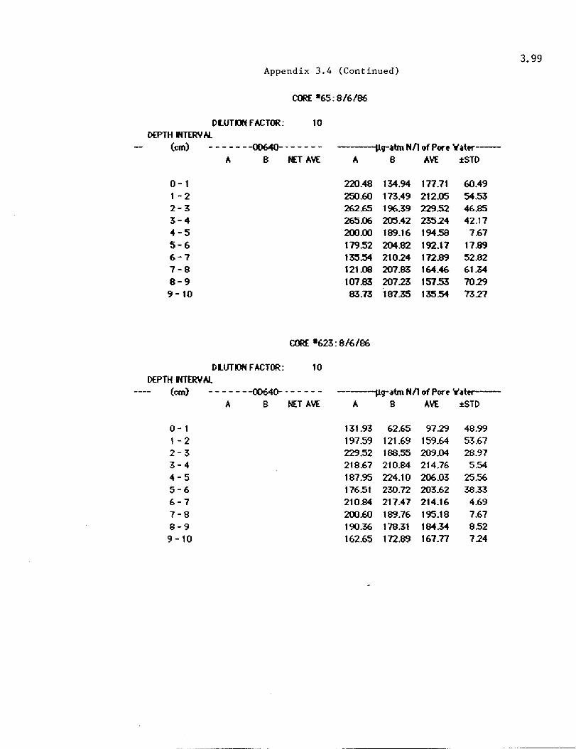
Appendix 3.4 (Continued)

CORE -65: 8/6186

OLUTDi fACTOR: 10 ()£PTH wrERY N...

(em) -------~.----- -----p.q-atm Nil of Pore .... ater---A B NET AVE A B AVE :tSTD

0-1 220.48 134.94 177.71 60.49 1-2 250.60 173.49 212.05 54.53 2-3 262.65 196.39 229.52 46.85 3-4 265.06 205.42 235.24 42.17 4-5 200.00 189.16 194.58 7.67 5-6 179.52 204.82 192.17 17.89 6-7 1~.:H 210.24 172.89 52.82 7-8 121.08 207.83 164.46 61.34 8-9 107.83 207.23 157.53 70.29 9 -10 83.73 187.35 135.54 73.27

CORE -623: 8/6/86

DLUTIOHFACTOR: 10 DEPTH MERYN...

(em) - - - - - --00640-' - - - -- -------;.tq-~tm Nil of Port .... at_--

0-1 1 - 2 2-3 3-4 4-5 5-6 6-7 7-8 8-9 9 - 10

A B NET AVE A

131.93 197.59 229.52 218.67 187.95 176.51 210.84 200.60 190.36-162.65

B

62.65 121.69 188.55 210.84 224.10 230.72 217.47 189.76 178.31 172.89

AVE :t:STD

97.29 48.99 159.64 53.67 209.04 28.97 214.76 5.54 206.03 25.56-203.62 38.33 214.16 4.69 195.18 7.67 184.34 8.52 167.77 7.24

3.99

Appendix 3.4 (Continued)

Core #45 - 8/6/86

Depth Interval (em)

o - I

1 - 2

2 - 3

3 - 4

4 - 5

5 - 6

6 - 7

7 - 8

8 - 9

9 - 10

3.100

!!g-at NLI of Pore Water A B Ave. ±STD

124.70 124.70

150.60 122.74 136.67 19.70

242.47 242.47

211.45 211.45

168.67 211.69 195.18 37.49

286.14 286.14

Appendix 3.4 (Continued)

CORE 1l613: 8/6/86

DLUHJN FACTOR: 10 DEPTH INTERYAl

(em) -------~.----- ll9""atm Nil of Port I(ater A B NET AVE A B AVE :tSTD

0-1 91.57 90.36 90.97 0.86 1 - 2 134.33 116.87 125.60 12.35 2-3 15422 123.49 138.86 21.73 3-4 149.40 11928 134.34 21.30 4-5 16325 124.70 143.98 2726 5-6 171.08 117.47 14428 37.91 6-7 15723 120.48 138.86 25.99 7-8 158.30 134.94 146.62 16.52 8-9 143.37 121.08 13223 15.76

9 - 10 139.16 121.69 130.43 12.35

CORE 8633: 8/6/86

DLUTION FACTOR: 10 DEPTH IHTERIr' At.

(em) - - - - - - -oD64O- • - - - - - -------;.t9""atm Nil of ~ I(ater-----

0-1 1 - 2 2-3 3-4 4-5 5-6 6-7 7-8 8-9

9 - 10

A B NET AVE A

139.76 240.36 300.00 315.06 310.84 31325 305.42 315.06 337.95 31626

B

126.51 239.76 289.76 348.80 328.31 336.14 354.82 355.42 367.47 368.67

AVE ±STD

133.14 9.37 240.06 0.42 294.88 724 331.93 23.86 319.58 12.35 324.70 16.19 330.12 34.93 33524 28.54 352.71 20.87 342.47 37.06

3.101

Appendix 3.5. Ammonium Concentration in the Water Column

Station • Nov'84 Jan'85 Mar'8S Apr'8S May'8S

45 603

65 613

85 623 633

0,59 5,26 2.47 0,72 2,98 0.79 0,55 6,01 1.18 0.62 0.90 0.45 0.71 0.42 0.36 1.38 0.42 0.39

0.19

Units· .Ilg-atm N per 1. Data from J. Cullen

0.09 0,28 0.04 0.17 0.03 0,16 0.Q2 0.03 0.10 0.83 0.01 0.17 0.02 0.67

Jun'8S

0.58 0.12 0.09 0.00 3.37 1.33 0.81

Ju1'8S AU9'8S Oct'8S Dec'85 Feb'86

0.41 0,16 0.08 0,66 0.62 0.19 0,14 0,27 0.34 0.46 0.19 0.16 0.01 0.36 0.44 0.17 0.29 0.01 0.47 0.81 0.31 0.85 0.50 1.24 0.84 0.27 0.21 0.18 0.53 0.84 0.25 0.36 0.13 0.31 2.04

Apr'86 Jun'86 Aug'86

0.04 2.89 0.64 0.08 0.47 1.45 0.08 2.20 0.64 0.14 0.99 0.57 0.31 0.73 1.21 0.14 0.97 0.50 1.26 0.54 0.78

w . ...... ~

Appendix 3.6. Measued AID ....... . flux st.tt •• ·85 C ...... r Experi_ab

Semple - - - - - - - - - - - - - - - - NH4-FlUX*- - - - - - - - - - - - - - - -Date

---(Jlv-atm N ~r I per h)--- - - - -- -(Jlg-etm N per m2 per h)-- ---Ch"'l Ch"'2 AVE Ch"'l Ch"'2 AVE ±STD

VEAR "'I 11128/84 0.24 2.04 1.14 65.1 545.0 305.\ 339.3

1123/65 0.59 -0.66 -D.05 160.1 -161.7 - 10.6 241.7 3/6/65 6.28 9.54 6.91 2247.4 2546.5 2398.0 212.9 4/3/65 -0.34 -0.36 -0.35 -92.3 -96.2 -94.2 2.7 5/8/85 0.31 0.21 0.26 64.1 56.1 70.1 19.8 6/5/65 0.47 0.41 0.44 133.2 114.4 123.6 13.3

7117185 0.00 -0.05 -0.03 0.0 -14.0 -7.0 9.9 6/14/65 ** ** ** ** ** ** "''''

YEAR "'2 10123/65 2.14 2.70 2.42 606.5 753.7 680.1 104.0 1214/65 3.24 3.95 3.60 918.3 1102.6 1010.5 130.3 2/5/86 4.33 5.63 5.08 1227.2 1627.4 1427.3 283.0 419/86 1.56 1.56 442.1 442.1 6/4/86 0.59 4.29 2.44 167.2 1197.5 682.4 728.5 6/6/86 0.07 2.02 1.05 19.8 563.9 291.9 384.7

* "-" = net NH4 flux INTO ~iment from 'w'tIter column; "+" = net flux OUT OF sedi meot into 'w'tIter col umn.

u Sampl~ lost.

Unib: Ammonium flux 8$ either 1) Jl9-etm N per l1ter of pore vater per hour or 2) JlQ-atm N per mA 2 of sediment per hour.

3.103

Appendix 3. 7. Theoretical Ammonium Flux

Station • Nov'84 Jan'85 Mar'65 Apr'85 May'85 Jun'85 Jur85 Aug'65 Oct'85 Dec'85 Feb'86 Apr'86 Jun'66 Aug'66

45 603

65 613

85 623 633

462.2 519.8 4.7 36.4 74.5 6,3 11.2 770.8 484.2 75f.3 455.4 431.3 151.0 515.9 848.2 5.0 6.1 7.6 5.6 27.0 29.5

75,2 285.8 185.0 110,5 302.8 298.8 328.0 104.4 88.9 27.4 35.6 6/.9 9.0 101.5 897.5 339.8 496,1 488.5 340.9 456.8 486.4 568. 1 9.4 2.2 5.0 38.5 3,6 31.0 539.6 410.0 724.0 458.6 188.6 129.6 322.2 62.6 34.6 24.5· 49.7 3.2116.1 941.5 48f.7 626.4 326.3 40.3 660.6 486.7 122.4 5.8 3.6 4.7 69.1 /75.3

825.5 95.4 95,4 83.9 f058.4 240.8 10.8 13.3 10.6 221.8 60.6

Units· ).Jg-atm N per m"2 per h. Theoreliclll ammonium nux calculated from pore waler ammonium gradient:

Method 1 Calculated from linear increase in ammonium concentration with increasing depth. Method 2 Calculated from nonlinear increase in ammonium concentration with depth, t1t1t1tori 3 Calculated from theoretical gradient resulting from difference in ammonium concentration in top

sediment segment and ammonium concentration in overlying water column.

w ..... o -I'>

CHAPTER 4

ZOOPLANKTON

INTRODUCTION

4.1

Zooplankton sampling was conducted to monitor the effects of freshwater

inflow on the spatial and temporal distribution of zooplankton at seven

stations in upper Lavaca Bay from November 1984 through August 1985 (Year

I) and October 1985 through August 1986 (Year 2). In Year 2, sampling effort

was increased to cover marine input from the lower bay by adding six stations

along a transect from state highway 35 causeway south along the Matagorda

Ship Channel to markers 35 and 36. Historical and concurrent stream flow

data indicate that Year I was a wet year and Year 2 was a drier year.

Zooplankton data reflect these differences.

METHODS

Zooplankton surface samples were collected in duplicate at each station

with the exception of the river stations 45 and 65 where a third oblique tow

from the bottom to the surface was taken during Year 2. Tows were not

replicated at stations I, 2, 3, 1505, 1905, and 35-36 during Year 2. A 0.5 m

diameter # I 0 mesh (153 /-1m) plankton net equipped with a General Oceanics

2030R flowmeter was used for sampling. Tows were of one minute duration.

Ctenophores collected were volumetrically measured then dissolved in a weak

solution of chlorox and washed through the plankton net to retain any other

zooplankton which may have adhered to the jelly. Plankton samples were then

washed into a I liter jar and preserved with 5% buffered formalin.

4.2

Zooplankton densities/m3 were determined from species counts of aliquots

taken with a Hensen-Stemple pipette. Each sample was diluted to a measured

volume (200 to 500 ml) and subsampled twice. The first sample (1 to 10 ml)

was used to determine the most abundant organisms, and the second (10-20 ml)

was used to estimate organisms not represented in the first subsample. The

remainder of the sample was then scanned at 12X for the larger, usually less

abundant zooplankton. Aliquots were placed in a Ward zooplankton counting

wheel and examined with a dissecting microscope at 25X. Triplicate 10 ml

subsamples were taken from replicate A for dry weight. These samples were

filtered onto a pre-weighed glass fiber filter, dried at 60°C for 24 hours, and

weighed using an analytical balance.

Statistical analyses included linear regressions and Spearman correlations

to test for the significance of freshwater inflow and salinity at stations 45, 65

and 85 and for Acartia tansa length versus salinity correlations.

Organisms were identified to species where possible. Counts and biomass

measurements are reported in numbers per cubic meter of water sampled. A

zooplankton species list is given in Table 4.1.

RESULTS

Community Description

Zooplankton total abundance for Year I and Year 2 is presented in Table

4.2. Although there was a major difference in inflow into upper Lavaca Bay

for the two sampling periods, there was basically no difference in the overall

zooplankton average standing crop for stations 45 through 633. On the basis

of these data the upper bay stations are characterized throughout most of the

year as having low densities. During this study, highest densities in the upper

4.3

bay occurred in the summer months of June 1985 and August 1986. These

density peaks occurred at stations 623 and 633. Additional data from stations

established in Year 2 depict a zone of· higher zooplankton abundance associated

with a salinity gradient from the upper to lower bay. These data will be

presented in detail under another topic.

Zooplankton dry weights (mg/m3) by stations are listed in Table 4.3.

Since formalin preservation results in a significant loss of dry weight, the

weights for zooplankton were adjusted by adding a 29.5% correction factor to

the original dry weights (Durbin and Durbin, 1978). Stations 45, 65, and 603

in close proximity to the major source of freshwater inflow, were consistently

lower than other sites. Biomass weights overall for the upper bay were higher

in Year I than Year 2. During Year 1 environmental factors, i.e. high wind

and freshwater inflows, increased the detritus and sediment load in the water

column which resulted in artificially higher biomass weights at certain stations

(Table 4.3). Secchi disc measurements (Fig. 1.5) are also indicative of higher

sediment and detritus loads in the water column in Year I. Attempts were

made to develop a correction factor for stations with detritus but apparent

variation in weight of different species of zooplankton made it unfeasable. In

Narragansett Bay, Rhode Island zooplankton collected on the same day from

different stations sometimes showed significant differences in weight for a

given length (Durbin and Durbin, 1978). The differences In the condition

factor appeared to be related to food availability.

The average weight per individual zooplankter in Lavaca Bay was 0.017

mg. When this value was used as a correction factor the biomass at some of

the stations with large amounts of detritus decreased while others increased.

The weight of 0.017 mg was comparable to adult weights for Acartia tOllsa

4.4

which range from approximately 0.01 mg for adults to 0.005 mg for first stage

copepodites (Miller et al., 1977). A correction factor which may be adequate

for one species, i.e. A. tOllsa, is not adequate when other species with

different weights are represented in a sample.

During Year 2 sediment loading was not a problem and biomass

measurements were usually indicative of zooplankton standing crops. With few

exceptions the upper bay biomass was always lower than the stations south of

the state highway 35 causeway.

Inflow Effects

The presence of freshwater zooplankton is indicative of freshwater inflow

into the study area prior to or during a sampling trip and the extent of spatial

distribution of freshwater species throughout the study area relates to the

magnitude of the event. From March 1985 through May 1985, persistent low

salinities allowed the dispersal of a freshwater zooplankton community

throughout the upper bay (Table 4.4). A decline in numbers of freshwater

species was evident from June 1985 through August 1986 with the exception of

minor influxes of freshwater species in December 1985 and June 1986. Inflow

events in December 1985 and June 1986 were small compared to flood events

from March and May 1985 and were restricted principally to river stations 45

and 65 and lake stations 603 and 613.

Due to the shallow depth of most stations, only surface plankton tows

were made with the exception of stations 45 and 65 in the river where depths

of 4.5 and 4.9 m were measured. On occasion, stratification was noted at

these stations, so in Year 2 an additional oblique tow was added to check for

zooplankton stratification (Table 4.5). These data present surface standing

crop abundance versus abundance for oblique tows and their relation to salinity

4.5

and oxygen, which can be used to verify stratification. In October 1985

(stations 45 and 65), December 1985 (station 65) and in June 1986 (station 65),

stratification was evident from salinity measurements and was also apparent

from the surface and oblique tow standing crop values. Lower standing crops

were generallly associated with lower salinity surface waters while higher

counts of estuarine species were found in bottom water. In June 1986,

stratification resulted in low dissolved oxygen below 1.0 m at stations 45 and

65. Standing crops were low in the surface and subsurface waters at station

45 while higher standing crops were found subsurface at station 65. These

data support the stratification conditions at the deeper river sites as noted in

the hydrographic sections of Chapter 2.

The incremental increase of estuarine and the decrease of freshwater

zooplankton with distance, starting from the source of freshwater (station 45)

and going downriver (station 65) to the open bay (station 85), is shown in

Figure 4.1. Obvious trends are for estuarine zooplankton to decline, especially

upriver during periods of peak inflow. Freshwater species increase during the

inflow events and decrease in density as they move downstream. The results

of linear regressions with estuarine and freshwater zooplankton, versus salinity

and inflow, and inflow versus salinity using Spearman Correlations are as

follows:

Spearman Correlation

Variables Stations: 45 65 85

Streamflow vs. -0.7 -0.91 -0.68 Salinity <0.005 <0.0001 <0.008

Salinity vs. 0.42 0.77 -0.15 Estuarine species <0.002

4.6

Salinity vs. -0.76 -0.92 -0.74 Freshwater species <0.002 <0.0001 <0.0003

Streamflow vs. -0.67 -0.71 -0.26 Estuarine species 0.009 <0.005

Streamflow vs. 0.93 0.94 0.7 Freshwater species <0.0001 <0.001 <0.005

These tests indicate that changes in response to inflow and salinity on

standing crop values of estuarine and freshwater zooplankton are significant in

most cases at the river stations 45 and 65 and at station 85 which is the

nearest open bay station to the river mouth.

Species Accounts

Acartia tansa was the most abundant copepod collected during this study

and in most other estuarine zooplankton studies. Abundance, spatial and

temporal distributions for A. tansa are shown in Table 4.6. A. tansa was

found throughout the study at all stations with the exception of surface tows

at station 45 in March and May 1985 when the streamflow was highest, 926

c.f.s. and 1913 c.f.s. and the salinity was low, 0.8 and 0.2 %0 respectively. The

lowest densities were associated with the lower salinity stations 45, 65 and

603. Highest seasonal densities in the upper bay occurred in the summer

months of June 1985 and August 1986 at stations 623 and 633. These peaks

correspond to the peak densities for the total zooplankton standing crop.

Apparent seasonal lows were in the winter or early spring months of March

1986 and February 1986 in the upper and lower bay. It is difficult to

distinguish between salinity related lows and normal seasonal lows in the upper

bay since this area is subject to periodic freshwater flushing. The upper bay

lows for A. tansa were associated with salinities from 0.5 to 6.4% in March

1985 and from 5.3 to 13.6%0 in February 1986.

4.7

A bloom of A. (onsa occurred at the lower bay stations in April 1986 but

was not evident in the upper bay.

In Year 2 A. (onsa was always more abundant in the lower than the

upper bay, with the exception of August 1986 where a bloom of A. (onsa was

found at stations 633 and 623. Note that the upper bay was recovering from a

freshwater inflow event in June 1986 and the salinity at stations 623 and 633

was 9.8 and 8.9 respectively. These salinities were at the low end of the

salinity range for the ctenophore, Mnenopsis mccradyii, a copepod predator;

which was at peak abundance at station 85 and most of the lower bay. High

densities of M. mccradyi in the lower bay may have been responsible for this

A. (ansa density shift.

The total length of approximately 20 adult A. (ansa males and 20 females

with spermatophores attached were measured at each station from October 1985

through August 1986 to test for a length relationship along a salinity gradient.

Measurements were taken from the tip of the prosome to the end of the 5th

thoracic segment at 50X using an ocular micrometer with a dissecting

microscope. The salinity ranged from 0.1 to 35.2%0. Female lengths ranged

from 0.56 to 1.0 mm with a mean of 0.7mm and the male lengths ranged from

0.48 to 0.88 mm with a mean of 0.62 mm. Linear regression of length versus

salinity demonstrated a significant length increase with salinity increase (P <

0.0005; Figs. 4.2-4.3). Three dimensional graphs (Figs. 4.4-4.5) indicate two

peaks for males and females, one at low salinity of small individuals and one

at higher salinity of larger individuals.

The ctenophore, Mnemiapsis mccradyi, a zooplankton predator, was absent

or in low numbers in the upper bay from November 1984 through June 1985

during persistent low salinities (Table 4.7). Highest density occurred in August

1985 and 1986.

4.8

In August 1985 it was found upriver to station 65 and

throughout the rest of the upper bay while in August 1986 its distribution was

from the lower bay up to station 85. Although similar salinity was

encountered in the upper bay during August 1985-1986 (Table 2.3), ctenophore

colonization was more wide spread in 1985 at the time of sampling. The

presence or absence of ctenophores from an area may affect zooplankton

density as was hypothesized to explain the decreased A. tonsa densities in the

lower bay in August 1986.

From October 1985 through August 1986, a 24-mile-long transect was

sampled from station 45 near the source of freshwater inflow along a gradient

to markers 35 and 36 in the Matagorda Ship Channel which were usually

influenced by marine input from Pass Cavallo and the Matagorda Ship Channel.

When average zooplankton densities for Year 2 by station are plotted from

station 45 to 35-36 along the salinity gradient, the trend is for zooplankton

density to increase from upper bay to the lower bay (Fig. 4.6). Salinity,

densities of freshwater zooplankton, and the most abundant estuarine and

marine species are plotted in Tables 4.8-4.10. Freshwater species abundance

increased in December 1985 and June 1986 at stations 45 and 65 corresponding

to surface salinities of 0.8 and 1.4, and 0.6 and 1.0 0100 respectively.

Throughout the year, typical estuarine species, I.e. barnacle nauplii, Acartia

tonsa. Paracalanus crassirostris. Pseudodioptomus coronatus, and Oithona

colcarva, reached peak abundance in a mid-bay zone between the freshwater

and marine input. Incursions of marine fauna are indicated by the densities of

the marine species Sagitta sp., Oikopleura, and Noctiluca scintillans. In

October 1985, densities of the larvacean Oikopleura ranged from 0.l/m3 at

station 45 to 2,620/m3 at station 35-36. Noctiluca scintillans, a neritic

4.9

dinoflagellate, was collected only in February and April 1986 with densities

ranging from 0.1 at station 3 to 385,368/m3 at station 35-36 in February 1986.

CONCLUSIONS

Zooplankton occurrence and abundance m upper and lower Lavaca Bay

were effected by freshwater inflow events and seasonality. As reported in

previous studies (Holland et al. 1975, Gilmore et al. 1976, Matthews 1980, Kalke

1981) flood events in an estuarine system usually result in the physical

displacement of estuarine zooplankton with a population of freshwater species.

In most cases the event is short term and salinity increases allow displaced

estuarine species, i.e. Acartia tansa, to recolonize quickly. The occurrence and

distribution of freshwater zooplankton in upper Lavaca Bay from March

through May 1985 reflect the influence of persistent low salinities during Year

of this study. The two freshwater events associated with Year 2 that

occurred in December 1985 and June 1986, mainly affected zooplankton

populations at the river and lake stations. Although freshwater inflows were

high in Year I compared to Year 2, there was no discernable difference in

zooplankton numerical abundance between the two years. The seasonal highs

for zooplankton abundance in the upper bay obviously occurred during the

summer months of June 1985 in Year I and August 1986 in Year 2 as shown in

Table 4.2. Seasonal cycles in the upper bay are sometimes difficult to

ascertain because sporadic freshwater inflow events usually result in decreased

zooplankton densities.

Zooplankton dry weight biomass measurements in most cases were

indicative of zooplankton abundance. During Year I there were problems with

detritus and sediment in some samples due to heavy runoff and windy

4.10

conditions. Biomass results indicate that the river stations 45 and 65, and the

upper lake station 603 are unstable in relation to zooplankton communities due

to periodic flushing with freshwater. As the nutrients are transported to the

bay and made available under more stable conditions, the resulting higher

zooplankton abundance increases biomass. According to biomass measurements

in Year 2, the estuary is organized in zones grading from low salinity areas

with low freshwater-estuarine zooplankton biomass, to a mid-bay zone with

estuarine-zooplankton of high abundance and biomass, to a higher salinity zone

of estuarine and neritic zooplankton which often has a biomass lower than the

mid-zone of maximum production.

The time of sampling in relation to the initiation and duration of a

freshwater event is important. For example, if this study had begun in

September 1984 the first trip would reflect conditions following a dry period;

whereas, we first sampled in November 1984 following a peak freshwater event

in October resulting in a freshwater signal. Freshwater zooplankton in an

estuary can be used as tracers to follow incursions of freshwater inflow

events. Estuarine and marine fauna can also be used to detect incursions of

higher salinity waters into low salinity areas.

A close relationship of zooplankton standing crop and Acartia tansa

density plots indicate the importance of A. tans a as a dominant estuarine

species. The lowest A. tansa abundances were associated with the river

stations 45 and 65 and the upper lake station 603 which were most influenced

by freshwater inflow. Relatively lower numbers of A. tansa and other

estuarine species in the upper bay during Year I indicated a need for expanded

coverage to the lower bay to define the zone of maximum zooplankton density.

Declines of A. tansa densities in the upper bay in March 1985 and February

4.11

1986 were probably a seasonal decline; however freshwater inflows in March

1985 may have also caused low densities. While the seasonal highs for A.

[ollsa in the upper bay occurred in June 1985 and August 1986, principally at

stations 623 and 633 some distance from the mouth of the river, a comparable

peak abundance in the lower bay area occurred in April 1986. These densites

remained relatively high but declined through August 1986. In August 1986 a

decline of A. [OilS a occurred in the lower bay, where densities were normally

higher than those in the upper bay. This decline may be related to the result

of ctenophore predation by Mllemiopsis mccradyi, which were abundant in

Matagorda Bay from station 1905 to station 85 in upper Lavaca Bay.

The total length of adult A. [ollsa males and females along a salinity

gradient may provide data which can be linked with optimal growth conditions.

Bagnall (1976) found A. [ollsa males and females in the Gulf of Mexico to be

larger than estuarine individuals from Christmas Bay near San Luis Pass, Texas.

Males were reported as being smaller than females and the largest individuals

occurred from February through May. Multiple regression of size on surface

water temperature and salinity did not explain a significant amount of

variation in size observed in either males or females (Bagnall 1976). Similar

results occurred in Lavaca Bay for male and female size differences, and a

significant positive correlation of increased lengths with increased salinity was

found. These data may be indicative of two different A. [Ollsa populations in

the same estuary or of size variations due to other environmental factors, i.e.

a temperature/salinity effect.

The greatest concentration of Mllemiopsis mccradyi in Lavaca Bay

occurred during the summer months of August 1985 and 1986 which corresponds

with large concentrations of copepods. The absence of Mllemiopsis from the

4.12

upper bay during most of Year 1 indicates a low tolerance for low salinity

conditions. Salinity increases during the August 1985 ctenophore bloom

expanded the distribution of Mnemiopsis up river to station 65, but during

their bloom in August 1986, low salinity in the upper bay above station 85

restricted distribution to the middle bay stations. Concentration of Acarlia

IO/lSa during August 1986 apparently decreased as a result of Mnemiopsis

predation in the lower bay, while peak densities of Acartia Ions a were found

in the upper bay in the absence of Mnemiopsis. Declines in zooplankton

standing crop in Sandy Hook Bay, N.J. in July and August, 1969 were

correlated with the presence of cnidarians and ctenophores (Sage and Herman,

1972).

Zooplankton data collected in Year 2 along a 24 mile transect from

station 45 to markers 35-36 were useful for determining extent of freshwater

inflow events and incursions of marine influence into the estuary. It also

made it possible to determine areas of maximum zooplankton standing crop and

biomass. In Table 4.8 through 4.10, freshwater inflow events in December and

June 1986 were minor and mainly influenced areas associated directly with the

river, i.e. stations 45 and 65. Streamflow data shows that increased inflow the

week after our June 1986 sampling trip was more extensive and most likely

influenced areas beyond the river mouth. Periods of low river flow, i.e.

October 1985, February and April 1986, result in higher salinities upriver and

the encroachment of estuarine and marine species into the upper bay and river.

One example is the distribution of the marine species, Oikopleura sp. in

October 1985, from a high of 2620/m3 at station 35-36 to 0.l/m3 at station 45.

As indicated by biomass during Year 2, distribution of freshwater,

estuarine and marine zooplankton partitions the estuary into three zones. The

4.13

upper zone near sources of freshwater inflow is subject to sporadic

environmental changes associated with salinity changes and the physical

displacement of zooplankton communities by freshwater flood events. Estuarine

species compete with fresh and brackish water species in this zone of low

salinity tolerance.

In a middle bay zone the salinities are normally more stable resulting in

a buffer zone between the upper low salinity and lower high salinity marine

environment. The area which represents this zone in Lavaca Bay is

approximately between stations 85 and 1905. The most common zooplankton in

this zone are considered estuarine species, i.e. barnacle nauplii, Acartia tonsa,

Paracalanus crassiortus, Pseudodiaptomus coronatus, and Oithona colcarva. The

highest concentrations are normally found within this zone.

The lower zone, of which station 35-36 seems to be on the inner edge of,

is exposed to marine input from the Matagorda Ship Channel and Pass Cavallo.

Although high densities of some estuarine species occur here it also supports

numbers of marine species associated with the neritic waters of the Gulf of

Mexico. The extent to which marine species range into the middle and upper

bay is dependent on the salinity gradient established by freshwater inflow

waters.

REFERENCES

Bagnall, R.A. 1976. Definition and persistence of an estuarine zooplankton

assemblage. Houston: University of Houston, Texas, Dissertation, 139 p.

Durbin, E.G. and A.G. Durbin, 1978. Length and weight releationships of

Acartia c!ausi from Narragansett Bay, R.I. Limnol. Oceanogr. 23(5):958-

969.

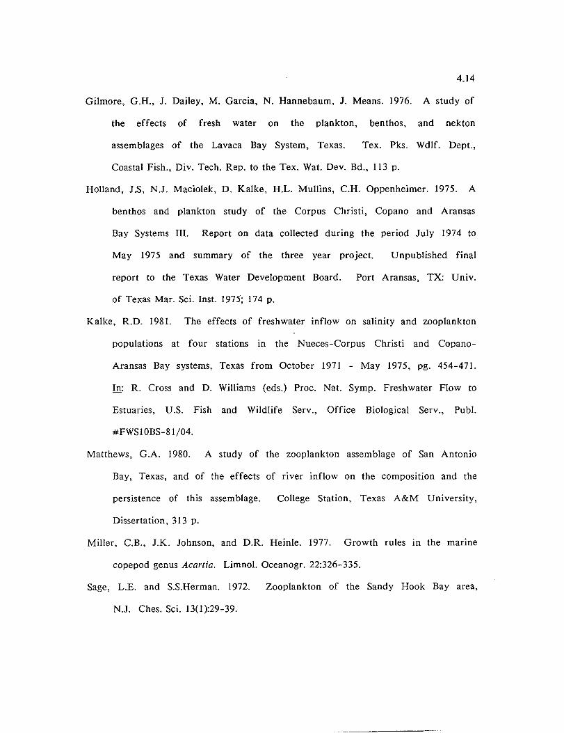
4.14

Gilmore, G.H., J. Dailey, M. Garcia, N. Hannebaum, J. Means. 1976. A study of

the effects of fresh water on the plankton, benthos, and nekton

assemblages of the Lavaca Bay System, Texas. Tex. Pks. Wdlf. Dept.,

Coastal Fish., Div. Tech. Rep. to the Tex. Wat. Dev. Bd., 113 p.

Holland, J.S, N.J. Maciolek, D. Kalke, H.L. Mullins, c.R. Oppenheimer. 1975. A

benthos and plankton study of the Corpus Christi, Copano and Aransas

Bay Systems III. Report on data collected during the period July 1974 to

May 1975 and summary of the three year project. Unpublished final

report to the Texas Water Development Board. Port Aransas, TX: Univ.

of Texas Mar. Sci. Inst. 1975; 174 p.

Kalke, R.D. 1981. The effects of freshwater inflow on salinity and zooplankton

populations at four stations in the Nueces-Corpus Christi and Copano­

Aransas Bay systems, Texas from October 1971 - May 1975, pg. 454-471.

In: R. Cross and D. Williams (eds.) Proc. Nat. Symp. Freshwater Flow to

Estuaries, U.S. Fish and Wildlife Serv., Office Biological Serv., Pub!.

#FWSI0BS-81/04.

Matthews, G.A. 1980. A study of the zooplankton assemblage of San Antonio

Bay, Texas, and of the effects of river inflow on the composition and the

persistence of this assemblage.

Dissertation, 313 p.

College Station, Texas A&M University,

Miller, C.B., J.K. Johnson, and D.R. Heinle. 1977. Growth rules in the marine

copepod genus Acartia. Limno!. Oceanogr. 22:326-335.

Sage, L.E. and S.S.Herman. 1972. Zooplankton of the Sandy Hook Bay area,

N.J. Ches. Sci. 13(1):29-39.

N u

III

IJ

t!

II t!

C

\I

1000(10

11.11 II III

1 I 1(1\ ~

1111)

4.15

[sluorine zooplonkton obundonce 1984 - 1986 2000

c

j 00(1

:~()O I

e 40(1 c

200

m 0

N 1 OI=:C'C~

II

III

b 1000

e r

100

Jl e

10 r

c II

III (I

r'~o:, ',' - .J,r.- I 1-=:.r- A~,t-- r-1,:,'ol - .Jun- .JIJj- AIJ'J- 00:\- (:":(;- F .'t.- A~.r- .Jur.- i~'J'J -,-,C" :=:c; :::5 ,-.C" : -.c :3:, ::--,;C; .-.c::- :::~. :~:(. :::f:. :36 - - '-'--' :'"-' . .: .. ,

Freshwater zoopl onklon obundance 1984 - 1966

i ~ 1401=; L

85 86

Figure 4.1. Total abundance of estuarine and freshwater zooplankton species vs. the 14 day average streamflow for stations 45, 65, and 85 from November 1984 through August 1986.

U

l e n Q ( t-

1.1

1.0

0.9'

0.8

0.7

: . . : : . !.

--. ._-. : : :. .. --.. ::. :: :-=----:--:--.... --OIl _OIl" .. _ .. _~ .. • .. OIl ... ___ OIl .... ~ ..

:::~._ ... -_OIl. .....-- __ ..... _ - _. -_.. .. - .. - - .- .- .. .. --- _ .. -... _-- .... ~ :: :: :=.: = :=: =:=: : .

:

0.6 .. .. -. ..

O.5i---------1---------Tl·---------,r---____ ~ o 10 L-o 30

Salinity

Data File: F€'mdata. S-w

Vac-idble Std. Err. t Name CoeftICient Estim.te Statistic

C«-, s t .1(1 t 0.66333 0.00363 182.95262 Salinity 0.00377 0.00010

O.ta File: Ferndat;; .5''''

S<:-urce

Model

ErrC'f"

Total

Sum of ()e.Q. of Near, S<:tuares Fr~om . Squares

1.S6S23 1.56823

6.06153 1370 0.00442

7.62975 1371

Coefficient ofOetenniMlion 0.20SS4 Coeftlcient of Correlation 0 _ 45337

Stdfldard Err« of Estimate 0 _ 06652

Durbin-Vatsoo Statistic' 0 _ 67093

18.826613

F-f:atio

354.44382

40

Prot. > t

0.000 0.000

Prob>F

0.000

4.16

Figure 4 - 2., Linear regres.sion of Acartia ~ female total length·vs. salinity for all stations from Octobei: 1985 through . Aug u·s t 1986.

900,------------------------------------,

BOO·

l e n Q ( h

x 700- ~~

--.~ ...... - .. - -~ ._-. 1 (I

600 - -- .. ---.. ~.---­~ .- ... ~ - ... - ..... - ---~-;...- - .-. ~:: :-.::: - :-

3: 50(1"

400 • • 0 10 20

Salinity

Oata File: Mal€'dat".5W

Vadable Std. EfT. Name CoeftICirot E~timate

. 3D

St. tis tic

Constant 0.55826 0.00287 194.74557 Salinity 0.00385

o .. t" File: MaI€'d"t".5'«

Sooroe

Model

Error

Tot,,1

Sum of DeQ. of Squares Freedom

1.46967 1

3.07228 1294

4.541% 1295

Coefficient of Detennin"tioo

CoeffICient of CorreL1tioo

Stat;dard Error of Estimate

Durl;in-\{ dL<oo Statistic

0.00015 24.87982

Medn Squares

1.46967

0.00237

0.32358

0.S6S84

0.04873

0.90011

F-Ratio

619.005L:S

40

Prof; > t

0.000 0.000

Proo>f

0.000

4.17

Figure 4.3. Linear regression of Acartia tonsa male total .length vs. salinity for all stations from OcobeJ' 1985 through August 1986.

c o u n ~ ,

80

L~ng~h

Figure 4,4,

'"'''''''''''''''' """',""" "',',' """,',"" ,,' "",',',',

""'''"'''' "'" "'" "'" "'" "'" "'" "'" "'" "'"

'\ •• ~. , • \ I '\ \. 'I,

t", '\. '\,.

35,3

Salinily

1,00 0,07

Three dimensional plot of Acartia tonsa female length data vs. salinity for all stations from October 1985 through August 1986.

-I'>

...... 00

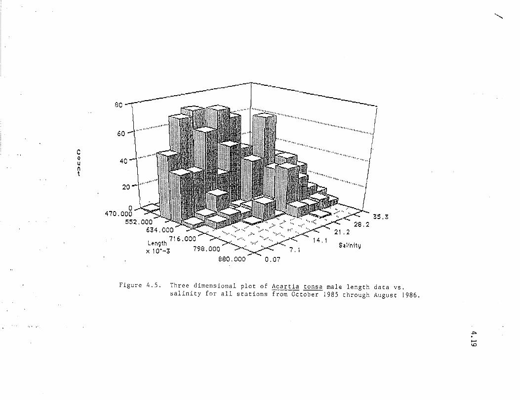
c o u

~

80

4 70, 008 ..--~:;! 552,000

634,000

L~n9th 716, 000 x 10'-3 798,000

880,000

,.,.,."""."""""""""""""""""

", " ", " ", " ", " ", " ", " "'" ", " ", "

"""."""""",.

Salinity

0,07

Figure 4.5. Three dimensional plot of Acartia tonsa male length data vs. salinity for all stations from October 1985 through August 1986.

.j:> -<D

'"

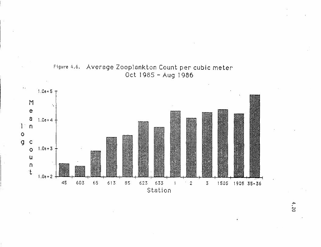
1.0e+ 5

M e a loOe + 4

n 0

9 c 0

u n t

Figure 4.6. Average Zooplankton Count per cubic meter Oct 1985 - Aug 1986

45 603 65 613 85 623 633 2 3 1505 1905 35-36 Station

.... N o

4.21

Table 4.1. Lavaca Bay Zooplankton Species List, November 1984 - Aug. 1986.

PHYLUM PROTOZOA Class Mastigophora

Order Oinoflagellata

PHYLUM COELENTERATA CI ass Hyd rozoa

CI ass Scyphozoa

Cl ass Anthozoa

PHYLUM CTENOPHORA Class Tentaculata

Cl ass Atentacul ata (Nuda)

PHYLUM PLATYHELMINTHES Class Turbellaria

Order Acoe 1 a

PHYLUM NEMERTINEA

PHYLUM ROTIFERA

PHYLUM KINORYNCHA

PHYLUM NEMATODA

PHYLUM ANNE UDA Class Polychaeta

Noctiluca scintillans

So lmari s sp.

Chrysaora quinquecirrha Stomolophus meleagris Medusae

Anemone

Mnemiopsis mccradyi

Beroe ovata

Fl atw0n11

Nemertean

Keratella sp. BrachlOnus pl icatil is Platyias quadricornis Platyias patulus Rotifer (unidentified) Rotifer (colonial form) Rotifer (large, soft body)

Kinorynch

Nematode

Polychaete larvae Autolytus prolifer

Class Oligochaeta

Class Hirudinea

PHYLUM MOLLUSCA Class Gastropoda

Class Pelecypoda

Class Cephalopoda

PHYLUM ARTHROPODA Cl ass Arachnida

01 igochaetes

Leech

Gastropod larvae Pteropoda

Pelecypod larvae

Loligunculus brevis

Order Acari na Hydracarina (water mites)

Cl ass Crustacea Order Diplostraca

Penilia avirostris

Sididae Diaphanosoma sp.

Daphnidae Ceriodaphnia sp. Daphnia sp. Moina sp. MOlnodaphnia sp.

Bo smi ni d ae 80 sm i na sp.

Macrothricidae Ilyocryptus spinifer Macrothrix sp.

Chidoridae Leydigea acanthoceroides Chydorus sp. Cladocera (unidentified)

Order Myodocopina Eusarsiella zostericola

Order Podocopa Ostracod (unidentified)

.4.22

Order Ca 1 anoida Calanoid (unidentified) Paracalanidae Paracalanus crassirostris Paracalanus sp.

Centropagidae Centropages hamatus Centropages velificatus

Diaptomidae Oiaptomus spp. Pseudodiaptomus coronatus

Calanidae Euca 1 anus sp.

Temoridae Eurytemora hirundoides Temora turbinata

Pontellidae Labidocera aestiva Labidocera scotti Pontella sp.

Acarti idae Acartia tonsa Acartia tonsa copepodids Acartia tonsa adults Acartia liljeborgii

Tortanidae Tortanus setacaudatus

Order Harpacticoida Ameiridae

Nitocra sp. Canuell idae

Scottolana canadensis

Harpacticidae

Metidae

Harpacticus sp. Zausodes arenicolus

Hetis sp.

Peltidi idae Alteutha depressa

Tachi idae Euterpinna acutifrons Mlcroarthridlon llttorale

4.23

Tegastidae Parategastes sp.

Unidentified Harpacticoid

Order Cyclopoida Oi thonidae

Oithona colcarva Oithona plumifera

Cyclopidae Cyclopoid copepodids Cyclops sp. Eucyclops agilis Eucyclops speratus Halicyclops sp. Henllcyclops sp. Macrocyclops albidus Mesocyclops edax Tropocyclops-prdsinus

Clausidiidae Saphirella sp. A (narrow) Saphirella sp. B (wide)

Ergasil idae Ergasilis sp.

Lichomolgidae

4.24

Lichomolgid A (Cyclopoid commensal)

Oncaeidae Oncaea sp.

Corycaeidae Corycaeus sp.

Sabell iphil idae Sabelliphilid sp. (Lubbockia)

Unident i fi ed Cyclopoid Copepodids Copepod Nauplii (Calanoid,

Harpacticoid and Cyclopoid combi ned)

Order Ca 1 igoida Cal igidae

Caligus sp. metanauplius Callgus sp.

Argulidae Argulus alosae

Order Thorac ica Barnacle nauplii Barnacle cypris larvae

Order Stomatopcda Stomatopod antiloea Stomatopod pseudoloea

Order Mys idacea Mys idae

Order Cumacea

Mysidopsis bahia Mys i dops is almyra MYSldopS1S sp. (juvenile) Metamysldopsis swifti

Cumacean (Juveni 1 e) Oxyurostylis salinoi Cyclaspis varTans---

Order Tanaidacea Leptochelia rapax

Order Isopoda Idoteidae

Edotea manto sa

Cymothoidae Aegathoa ocul ata

Bopyridae Bopyrid A

Munnidae Munna sp.

Order !lmphipoda Ampel isc idae

!Impel isca abdita

Amphithoidae Cymadusa compta

Bateidae Batea catharinensis

Corophi idae Corophium louisianum Corophlum acherUSlcum

4.25

Gammaridae Gammarus mucronatus Mlcroprotopus sp.

Oedicerotidae Monoculodes nyei

Caprell idae Caprellid (immature)

Order Decapod a Palaemonidae

Macrobrach i urn sp. Zoea Palaemonetes sp. Zoea Palaemonetes pugio

Al pheidae Alpheus sp. zoea Luc i fer faxoni Lucifer faxoni protozoea

Penaeidae Penaeus aztecus postlarvae Penaeus setiferus postlarvae

Se rges tid ae Acetes americanus louisianensis Acetes americanus louisianensis

protozoea

Ogyrididae Ogyrides limicola Zoea Ogyrides limicola post larvae

Ca 11 i anass idae Ca 11 i anassa sp. Zoea Ca 111anassa sp. juvenile Callianassa sp. Zoea #2 Porce 11 ani d Zoea

Upogebia affinis zoea

Hippo 1 yt i d ae Tozeuma carolinense zoea Hippolyte sp. zoea

Hippolysmata wurdemanni

Porcell anidae Petrolisthes armatus zoea Petrolisthes armatus megalops

4.26

Class Insecta

Paguridae Clibanarias vittatus zoea Pagurus sp. zoea Glaucothoe larvae

Portunidae Callinectes spp. megalops Cal1inectes sapidus

Xanthidae Rithropanopeus harrissi Zoea

Pi nnotheridae Pinnixa sp. Zoea Plnnotheres sp. Zoea Pi nnotherid zoea A

Ocypodidae Uca sp. Zoea

Unident i fi ed Brachyuran Zoea Brachyuran megalops Decapod larvae (Galatheid type)

Order Ephemeroptera Insect 1 arvae ~1ayfly larvae

Order Chironomidae Mi dgefl y 1 arave Midgefly pupae

Cl ass Tard igrada

PHYLUM PHORONIDA

PHYLUM ECHINODERMATA

PHYLUM BRYOZOA

Tardigrade (water bears)

Actinotroch larvae

Ophiopluteus larvae Echinopluteus larvae Bipinnaria larvae

Cyphonautes larvae A Cyhonautes larvae B

4.27

PHYLUM CHAETOGNATHA Saggita sp.

PHYLUM CHORADATA Class Ascidiacea

Ascidian larvae

Class Larvacea Oikopleura sp.

Class Osteichthyes Fi sh eggs

4.29

lavaca BalJ Table 4.2 Zooplankton abundance 1984 - 1966

1984 - 1985 (i ndividuabl m cubed) Station Nov-84 Jan-85 Mar-85 A r-85 MaIl-85 Jun-85 Ju1-85 Au -85 Average s.d.

45 379 3018 3294 158 608 279 62 382 1022.5 1328.8 603 1573 1255 657 66 74 1064 40 808 692.13 591.02

65 1742 1468 2316 40 200 705 322 548 917.63 824.6 613 7424 906 1801 2328 833 1722 56B 2279 2232.6 2200.6

85 3671 3656 1985 14220 2905 7781 2916 2074 4901 4185.4 623 3938 4515 983 1984 400 24440 3868 1417 5193.1 7923.7 633 7961 1218 2469 34889 6685 3061 9380.5 12762

Ave rage 1 3121.2 2469.7 2713.9 2859.1 1069.9 10126 2065.9 1509.9 3256 S.d. 2502.1 1470.7 2470.4 5096.7 1139.6 13917 2540 1001.2 5910

1985 - 1986 (i ndividu81~1 m cubed) Station Oct- 65 Oec-B5 Feb-86 A r-86 ,Jun- 86 AUQ-86 AveraQe S.d.

45 448 257 11 221 257 633 304.5 212.66 603 131 194 179 250 175 533 243.67 146.84

65 395 267 598 494 37 3'353 857.33 1238 613 482 1981 234 351 478 12171 2616.2 4725

85 2847 319 7447 4902 2235 829 3096.5 2677.6 623 3573 2861 1436 15840 2968 30585 9543.8 11590 633 102 2407 631 3244 191 28938 5918.8 11349

,5992 4580 77184 9600 12321 21935 31034 2 7766 15849 20314 10111 9775 12763 5183.4 3 5963 8093 48821 24971 11601 19890 17781

1505 38482 12686 33572 31900 22848 11465 25159 11333 1905 20716 7413 20346 22504 16197 20544 17953 5567.1

35-36 12633 8376 398108 6613 7130 86572 174170

Average 17980.9 4344.8 37776 18835 7437 11529 14664 s.d. 12711 3985.3 108734 23944 8856.3 9966.3 47071

Average st 45- 633 3226 S.d. 6796

4.30 Lavaca 8a'1

Table 4_3 Zooplankton biomass 1984 - 1986

1984 - 1985 (mg dry VIti m cubed) Station Nov-84 Jan- 85 Mar-85 A r-85 Mau- 85 Jun- 85 ,Jul-85 AUQ- 85 Average s.d.

45 1.0 7.0 5.6 2.6 3.2 3.4 1 ;, 3.0 3.4 2.0 603 52_1 1 L7 6.3 -'0 I.u 2.3 14.6 2.6 3.9 12.7 16.5

65 15_2 3 ~, .... 3.4 5.4 0.6 4.9 ~. c L.-." 4.9 5.0 4.4

613 390_2 49_9 0..., 36_8 7.6 8.2 13.0 R r. 65.3 132.2 LI.L _ .0

0:01:' C' c· 1? "1 1.3 69_':' c .:> ..1.e n 23.6 32.1 24.7 23.8 -~~I --'.'-' 10:... I "_'.U ""t;_I.'_'

I)L.:r 72_0 40.7 38.6 1473_8 24.3 158_8 44.5 17.5 233.8 503.0 6331 41.4 355_3 22.1 1 I) 1.7 17.9 16.Eo 92.5 132.7

AVer;Qel :39.4 20.8 15.0 278.8 9.5 40 ·c, 15.0 12.4 61.4 I_I.L

150.0 19.4 17.3 541.7 Q, 60.1 15.6 10.5 208.9 _ .. d. .",1

10AC: - 1 Q~~? ( riO" A'-II -.. _.i ..- r,o, .... '1 ... .:..-("'" . J'"'.J .... . ... ··.Jv '<.111':1 YI '; ",Y \i III vUlJ ..... UI

':;t&tiOri O(:t-85 Dec- 85 feb-86 A Ir-t:6 ~lun-86 AUQ- 86 Ave raae s.d. .ie 1 ~, • 7 -'") ...-, 6.0 0.4 1.0 2.0 2.0 .... ~. .~

i ___ ; L.L

hn~1 7 1 0.5 3.6 1.3 0.3 4.7 2.2 1.8 -:~I

__ I. ,

1 ? 1.0 0.6 6_7 3.4 7.1 '7 '7 2.9 tLJI ... ' .... 1

613! 1.8 7.3 26.7 1.3 ? ~. 19.2 Q -, 10.7 ~.L .-. I

85 13.3 13.7 2.6 17.0 3.6 22.9 12.2 7.8

623 12.0 7.5 17.9 55.0 10.7 175.2 46.4 65.5

633 -, '7 f • __ 1 27.6 6.7 28.4 ' ? D._ 53.9 21.7 18.9

28.0 87A 308.7 1 l'c, .:0 '::".1_' 23.3 1 12.0 1 16.4

.; 37.3 21.4 207.3 770 37.4 67.4 78.5 "- ...}._I.I_'

~ 7.8 14.1 220.9 B2.9 76.3 80A C' c c' - _::1 !.J .'_1

1 ::.u:., 18.5 21.6 1 12.7 82.:3 34.:3 54.1 41.7

1905 25.6 19.8 97.9 56.1 49.1 49.7 31.0

35-361 43.0 137.1 12.2 "';.'7 c, 54.0 56.8 L ..... '.IJ

.!!,verage! c -, 16.9 27.8 8:3.6 31.3 40.7 36.9 -J. I

~.d. I c ---:. 14.3 :z;.q Co 104.2 39.0 45.7 57.3 "_I.t.. -_ 4" .1..1

Average ~ 45-633 13.9 ::;.d . . ~ 45-~.d. 28.5

bold = Detritus in sample

4.31

Lavaca BalJ Table 4.4 Fre:shyater zooplankton abundance 1964 - 1966

1984 - 1985 (i ndividua131 m cubed) Station Nov-84 Jan-85 Mar-85 A r-85 Mau-85 Jun-85 Jul-85 Au -85 AveraQe s.d.

45 1.5 2985 3285 148 572 58 50 0.1 887.45 1401.8 603 1.5 666 358 9 17 23 1.3 0 134.48 247.26

65 3.4 1352 2096 33 73 0.5 3.5 0 445.18 814.35 613 0 104 81 41 70 0 1 0 37.125 42.983

85 0.1 0 45 57 25 0 0 0 15.866 23.542 623 o 1 1.5 19 56 69 0 0 0 18.2 26.31 633 c 84 252 0 0 57 101.09 oJ

Ave rage I 1.1 851.42 841.29 61.143 154 11.643 8.1143 0.0143 234.2 s.d. 1.3282 1169.9 1314.5 44.771 200.24 22.152 18.507 0.0378 673

1985 - 1936 (i ndividualsl In cubed) Station Oct-85 Dec-85 feb- 86 A r- 86 ~(un- 86 AUQ-86 AVer8Qe s.d.

45 0.1 159 0.2 0.1 255 0 69.067 111.07 603 0 61 0 0 0.8 0 10.3 24.84

65 (I 89 0 0 24 0 18.833 ~15.69

613 0 18 0 0 0.1 0 3.0167 7.3404 85 0 1 0 0 0.1 0 0.1833 0.4021

623 0 0 0 0 0 I) 0 0 633 0 0 0 0 0 0 0 0

0 0 0 0 0 0 (I ~, 0 0 0 0 0 0 0 L

3 0 0 0 0 0 0 (I

1505 0 0 0 0 0 0 0 0 1905 0 0 0 0 0 0 0 0

35-36 0 0 0 0 0 0 0

Average I 0.01 25.231 0.0154 0.0083 21.538 0 6.222

s.d. 0.0316 49.136 0.0555 0.0289 70.457 0 36.61

Average :It 45- 633 14.49 3.d. 47.69

4,32

l8V8ca 8811 Table 4.5 Surface and bottom $tandlDg crop V$ $tratlflcatloD

1985 - 1986 Od-85 Dec-85 Feb- 86 Apr- 86 JUfl- 86 Aug-86 t·1ean 14 d tlo ... · ... , (:u ftl3ec 33 521 43 "Z~

.Jt.. 258 15

Station 45 Standi ng crop, surface to'w' 448 257 11 221 257 '"z"z b .. }..}

45 surface sali nity, ppt 4.4 0.9 5.3 13.4 0.6 3.9 45 surface dissolved Oxygen,rng/l q-, .. , 9.9 9.5 9.5 8.2 7.4

45 stand1 ng crop, oblique to'vl 1524 7") --I I ;;... 264 539 456 2321

45 bottom sali nity., ppt 17.6 2.3 6.3 13.8 18.1 4.4 45 bottom di::;solved Ox llQen, m'l/l 1.4 9.7 7 9.5 0.3 5.6

65 StandirN crop, surface toW' 395 267 59B 494 37 3353 65 surface :;;alinity. r,~,t 6.9 1.4 8.7 16.1 1 9.4 65 :3lJrfaee di:5:';olved OX1J'~en,mg/l 6 10.2 9.8 8.9 8.2 8

65 stllndi ng (:rop, oblique to''; 1721 1287 588 625 2521 8953 65 bottom sali nitlJ, ~Ipt 17.7 8 13.1 17.4 18.3 9.9 65 bottom dissolved OXllaen mall 4 ;' 10.1 7.4 8.5 0.3 7.1

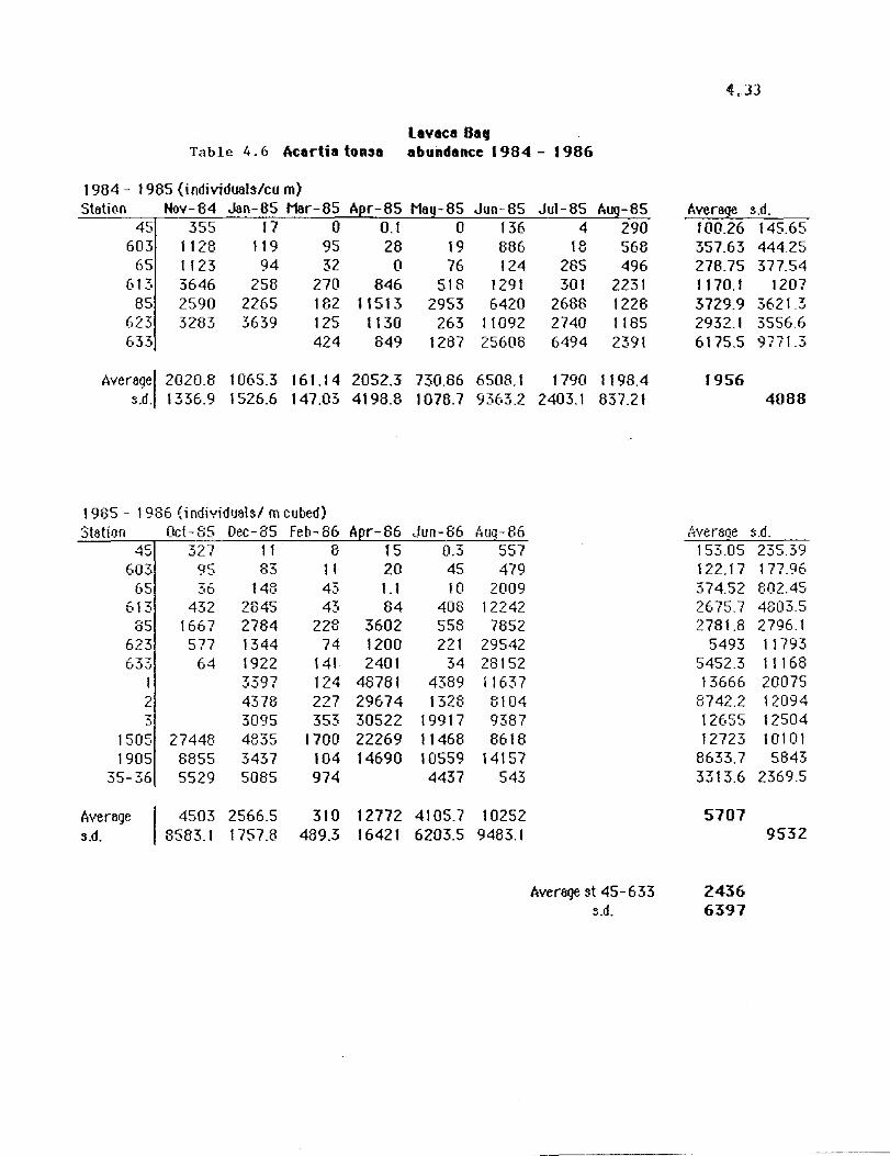
'¢.J3

lavaca 8a, Table 4.6 Acartis ton:ss abundance 1964 - 1966

1984 - 1985 (iodividuals/cu m) Station Nov-84 Jan-85 Mar-85 A r-85 Ma~-85 Jun-85 Ju\-85 A -85 Average s.d.

45 355 17 0 0.1 0 136 4 290 100.26 145.65 603 1128 119 95 28 19 886 18 568 357.63 444.25

65 1123 94 32 (I 76 124 285 496 278.75 377.54 613 3646 258 270 846 518 1291 301 2231 1170.1 1207

85 2590 2265 182 11513 2953 6420 2688 1228 3729.9 3621.3 623 3283 3639 125 1130 263 11092 2740 1185 2932.1 3556.6 633 424 849 1287 25608 6494 2391 6175.5 9771.3

Averagel2020.8 1065.3 161.14 2052.3 730.86 6508.1 1790 1198.4 1956 !i.d. 1336.9 1526.6 147.03 4198.8 1078.7 9363.2 2403.1 837.21 4086

1985 - 1986 (i ndividlJal3l m clJbed) Station Oct- 85 Dec-35 Feb- 86 A r-86 <.!un- 86 I~UQ- 86 {weraoe s.d.

45 327 11 8 15 0.3 557 153.05 235.39 603 95 83 1 1 20 45 479 122.17 177.96

65 36 148 43 1.1 10 2009 374.52 802.45 613 47? -.'L 2845 43 84 408 12242 2675.7 4803.5

35 1"7 bb. 2784 228 3602 558 7852 2781.8 2796.1 623 577 1344 74 1200 221 29542 5493 11793 633 64 1922 141 2401 34 28152 5452.3 11168

3397 124 48781 4389 11637 13666 20075 2 4378 227 29674 1328 8104 8742.2 12094 3 3095 353 30522 19917 9387 12655 12504

1505 27448 4835 1700 22269 11468 8618 12723 10101 1905 8855 3437 104 14690 10559 14157 8633.7 5843

35-36 5529 5085 974 4437 543 3313.6 2369.5

Average I 4503 2566.5 310 12772 4105.7 10252 5707 s.d. 8583.1 1757.8 489.3 16421 6203.5 9483.1 9532

Average st 45-633 2436 !i.d. 6397

4.34

Lavaca BaCJ Table 4.7 Hnemiop3i3 mccredCJi . abundance 1984 - 1986

1984 - 1985 (volume mil cu m) Station Nov-84 Jan- 85 Mar-B5 A r-85 Mall-85 Jun-85 ~lul-85 AUQ-85 AveraQe s.d.

45 1.3 0 0 (I (I 0 [I 0 0.1625 OA596 603 0 0 0 0 0 1) 0 0 [I 0

65 (I (I 0 (I 0 0 (I 70A 8.8 24.89 613 0 [I 0 0 [I 0 6.8 27 4.225 9.5051

85 [I [I 0 0 [I I) 48 54 12.75 23.663 623 0.4 I) 0 0 0 0

r , O? 09125 2.343 0." .7-j (I (I 0 (I 0 0 5.1 40 5.6375 13.999 t·._,,)

Averagel 0.2429 (I 0 0 0 (I 9.5143 27.371 4.641 s.d. OA894 0 [I 0 (I (I 17.26 28.743 14.41

1985 - 1986 (vol ume ml,' GU m) Station Oct- 85 Oec- 85 Feb-B6 • r-86 ~lun-86 AUQ- E:6 Averfloe c- ."i H ... ·.u. ..

45 u I) 0.2 0 0 (I 0.0333 0.081 Eo

603 " " (I 1.9 (I 0 (I 0.6B33 1.0629 L.L

65

1

(( 1.7 0.3 0 0.1 0.1 0.3667 0.6623 613 4 c 0 1.3 (I 0.2 I) 1.7;::77 ._'

.;:·c IJ.J 20 5.3 0 1.3 0.7 4" -L 1 1.55 16.696

623 19.5 10.2 0.1 0.1 0 I) 4.9i333 8.1891 633 80 13.4 " 1.5 0.6 (I 16.25 31.628 L

0.7 0.1 16 0.1 1 I 5.5B 7.4469 2 0.3 0.1 -: .... , 0.1 139 34.4 60.06 .JL

.. ' n '. .. L 0.1 0 (I 1 c· '.' 3.66 8.0167 1505 0.5 0.2 o c· .L'

?7 L.. ...... ' 0.1 29 5.4833 I 1.548

1905 0.6 0.5 0 17 0 14 5.35 7.9231 35-36 0.5 0 2.6 0.1 0 0.64 1.1 149

Average I 12.78 2.5385 0.7308 5.85 0.1538 19.469 6.697 s.d. 24.884 4.3995 0.9096 10.303 0.2295 38.34 19.71

Averagest 45-633 4.961 S.d. 14.19

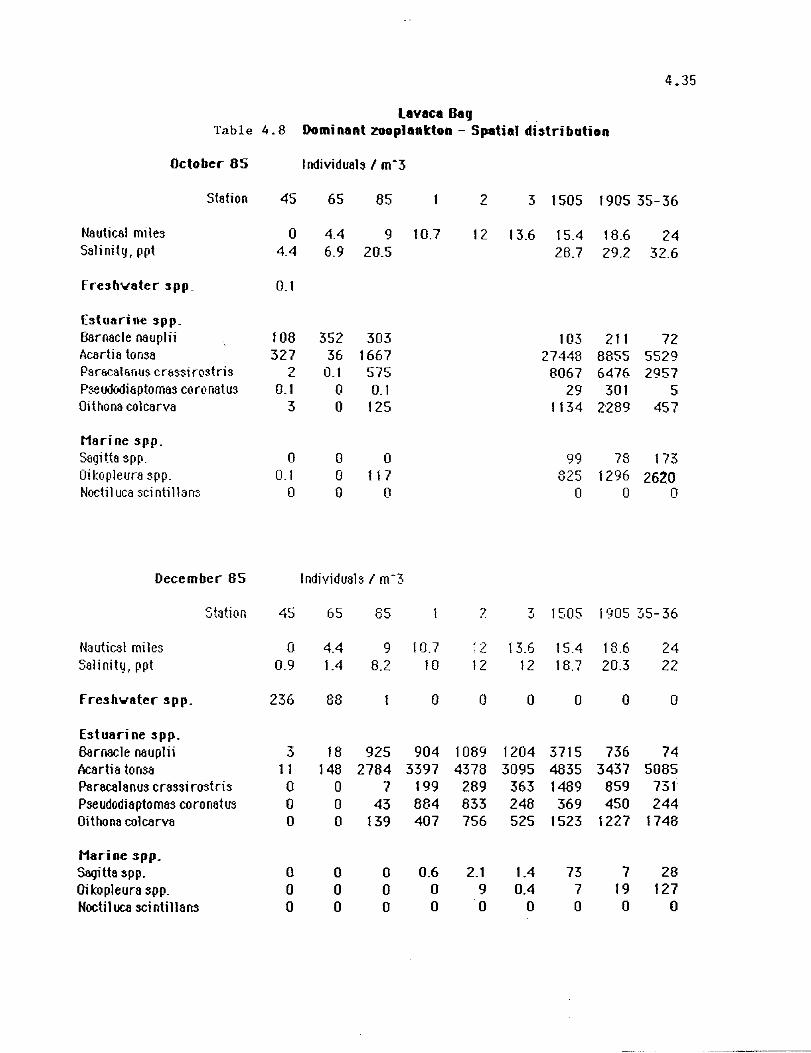
4.35

Lavaca Bay Table 4.8 Dominant zooplankton - Spatial distribution

October- 85 Individuab I mA 3

Station 45 65 85 2 3 1505 1905 35-36

Nautical mile3 0 4.4 9 10.7 12 13.6 15.4 18.6 24 SalinitlJ. ppt 4.4 6.9 20.s 28.7 29.2 32.6

freshv8ter spp_ 0.1

Estu8ri De spp_ Barnacle nauplii 108 352 303 103 211 72 Acartia ton3a 327 36 1667 27448 8855 5529 Psracslanus cr83sirostris ? 0.1 575 8067 6476 2957 ~

Pseudodiaptomas coronatu3 0_1 0 0.1 29 301 5 Oithona colcarva 3 0 125 1134 2289 457

Marine spp_ Sagitta 3pp. 0 0 0 99 78 173 Oi kopleura spp. 0.1 0 11 7 825 1296 2620 Nocti I uca sci nti 11 a rr<. 0 0 0 0 0 0

December 85 Individuals I m-3

Station 45 65 85 2 7 1505 1905 35-36 ..J

Nautical miles 0 4.4 9 10.7 ~ 2 13.6 15.4 18.6 24 Salinity. ppt 0.9 1.4 8.2 10 12 12 lB.7 20.3 22

freshvater spp_ 236 88 0 0 0 0 0 0

Estuari De spp. Barnacle nauplii 3 18 925 904 1089 1204 3715 736 74 Acartia tons& 11 148 2784 3397 4378 3095 4835 3437 5085 Paracalaous crassi rostris 0 0 7 199 289 363 1489 859 731 Pseudodiaptomas coronatu3 0 0 43 884 833 248 369 450 244 Oithons colcarva 0 0 139 407 756 525 1523 1227 1748

Marine spp. Sagi tta spp. 0 0 0 0.6 2_1 1.4 73 7 28 Oi k:opleura spp. 0 0 0 0 9 0.4 7 19 127 Nocti 1 uca sci otill a os 0 0 0 0 0 0 0 0 0

4.36

Lavaca BalJ Table 4.9 Dominant zooplankton - Spatial di3tribution

february 86 Individuals I m"3

Station 45 65 85 2 3 1505 1905 35-36

Nautical miles 0 4.4 9 10.7 12 13.6 15.4 18.6 24 Salinity. ppt 5.3 8.7 13.1 9.2 15 20 14.4 18.2 20.4

freshYater spp. 0 0 0 0 0 0 0 0 0

btuarine spp. Barnacle nauplii 1.4 534 7120 3766 15267 7513 13733 2374 8737 Acartia ton311 8 43 228 124 227 353 1700 104 974 Parocalaous crassi rostris 0 0 4 0.5 0.6 22 80 10 237 P~.eudodiaptomas coronatus 0.1 0.1 0.4 102 58 0.3 47 7 79 Oithooa colcarva 0 0.4 47 43 62 58 713 176 1605

Salt ..... 8ter spp_ Sagitta spp. 0 0 0 0 0 0.3 0.8 0.1 0 Oi kopleufa $PP. 0 0 0 (I 0 (I 0 .,- 79 ~,

Noctil uca scintillaos 0 0 0 0 (I 0.1 17067 17463 385368

.... pril 65 I ndividuals I m"3

Station 45 65 85 2 .. 1505 1905 ::,5- 36 ~,

Nautical miles 0 4.4 9 10.7 12 13.6 15.4 18.6 24 SalinitlJ. ppt 13.4 16.1 23.9 26 26 27.3 27.9 28.4

freshYater spp. 0 0 0 0 0 0 0 0

btuarine 3pp. Barnacle nauplii 198 469 647 24573 6250 10522 1111 1063 Acartia tonsa 15 1.1 3602 46781 2967430522 22269 14690 Paracalanus crassi rostris 0 0 0.1 31 16 299 417 0 Pseudodiaptomas coronatus 0.1 0.7 0.1 549 380 746 324 57 OitOOna colcarva 0 0 3 165 125 224 602 412

Salty.ter 3PP_ Sa9itta spp. 0 0 0 1.2 0.1 0.7 0.7 0.5 Oi I:opleura spp. 0 0 149 427 1957 746 926 1063 Noctil UCII sci ntillaRS 0 0 0 0 0 0 0 ISS

4,.31'

Lavaca Bay Table 4.10 Domi nant zooplankton - Spatial di:stri bution

.June 86 lodividuab I m'3

Station 45 65 85 2 3 1505 1905 35-36

Nautical miles 0 4.4 9 10.7 12 13.6 1 S.4 18.6 24 Salinity, ppt 0.6 18.9 21.8 20.7 26 26.7 Z7 28.1

rre:shvater :spp. 255 24 0

£:stuari ne :spp. Barnacle nauplii 0.5 0.9 1460 1727 3379 672 707 446 289 Acartia tonsa 0.3 10 558 4389 1328 19917 11468 10669 4457 Paracalanus cras!'oi rostris 0 0 1.3 0 4 168 271 670 4~5 Pseudodiaptornas coronatus 0 0 0.4 809 801 378 1848 580 44 Oithona colcarva 0 0 0.4 0 4 168 217 179 124

Saltvater 3PP_ Sagitta spp. 0 0 0 0 0 0.8 5 27 2 Oikopleura spr'. 0 0 0.4 4 8 210 2005 446 3 Noctil uca sci ntillans 0 0 0 0 (I 0 (I 0 0

i\U<jU3t 86 Individuals I m'3

StFJtion 45 65 85 2 7 1505 1905 35-36 J

Nautical miles 0 4.4 9 10.7 12 13.6 15.4 18.6 24 581i nily, ppt 3.9 9.4 II 16.1 18.7 21.3 24.2 26.1 35.3

fre3hvater :spp_ 0 0 0 0 0 0 0 0 0

£:stuari ne :SPIL Barnacle nauplii 41 403 292 303 1485 434 293 107 0 Acartia tonsa 557 2099 7852 11637 8104 9383 8618 14157 543 Paracalanu~ crassi rostris 0 0_1 L5 3 0 124 130 656 509 Pseudodiaptomas coronatu3 a 3 5 61 0 433 520 1406 8 Oithona colcarva a 0 31 76 6 247 553 1594 335

Sa1tvater :spp_ Sagitta spp. a 0 0 0 0 0.4 0 2_6 L6 Oil:opleura spp_ 0 0 0 0 0 62 98 250 5 Noctil uca sci ntillans 0 0 0 0 0 0 0 0 0

CHAPTER 5

BENTHOS

INTRODUCTION

5.1

Benthic macrofauna consisting primarily of polychaete worms, molluscs,

and small crustaceans are secondary producers associated with the sediment.

These organisms transfer energy from the primary producers, i.e. bacteria,

microphytobenthos, and the phytoplankton, to higher trophic levels. The

benthic macrofauna in the upper Lavaca Bay during this study was limited to a

few dominant organisms consisting of the polychaetes, Mediomastus

californiensis and Streblospio benedicti, Chironomid midge fly larvae, and the

molluscs Macoma mitchelli and Mulinia lateralis. A list of species collected is

given in Table 5.1.

METHODS

Benthic core sampling was accomplished using SCUBA or snorkeling.

Triplicate samples were collected at each site with 7.5 cm diameter, 30 cm long

aluminum cores which were capped and placed upright in a bucket of ambient

water. The walls of each sediment core were split to aid in sectioning the

sediment horizontally by depth.

Each core was sectioned at the following depths: 0-3, 3-10, and 10-20

cm. Sections were placed in a I liter jar and preserved with 10% formalin in

seawater stained with rose bengal. In the lab, each sediment section was

sieved through 0.5 mm mesh and the retained organisms were identified and

counted. Wet weight biomass was measured on dominant individuals and on the

entire sample.

5.2

The effect of freshwater inflow of Lavaca Bay benthos was determined by

analyzing bay-wide abundance and biomass with physical parameters, i.e.,

salinity and temperature (Table 5.2). The x 14 day Lavaca River streamflow

rate calculated from the U.S. Geological Survey data from streamflow gauge

number 08164000 near Edna, Texas was also used. The x 14 day flow period

was chosen to assess the impact on recent flow regimes on the fauna. Lagged

effects of flow were also examined. For example, benthic reproduction and

migration time is on the order of 1 month and a flow event may not result in

measurable short term changes m the benthic community. Pearson Correlation

Coefficients were calculated for benthos with salinity, temperature, x 14 day

flow and the x 14 day lag flow. The lag flow was achieved by shifting the

flow data forward by one sampling trip. Since Table 5.2 contains 50

correlation tests, it is prudent to take the Bon Ferroni approach and reject at

P = 0.001 (i.e., .05/50).

RESULTS

Distribution Patterns

The benthic community m upper Lavaca Bay is typical of a low to

moderate salinity environment with only a few dominant species. Very little

change was seen in the total benthic faunal abundance between Year 1 and

Year 2, but stations 623 and 633 had an abundance increase in Year 2 (Table

5.3). Monthly standing crop increases were evident in March and June 1985

and in February and April 1986. No significant calculations were found with

faunal abundance and any of the physical parameters measured (Table 5.2).

The distribution of infauna by depth in the sediment was typical for most

estuaries. Highest concentrations of organisms were found in the upper 0-3

5.3

cm, decreasing with depth with the lowest numbers found in the 10-20 cm core

sections (Table 5.3, Fig. 5.1).

for both years.

Average abundance within sections was similar

Benthic biomass was in direct contrast to the abundance distributional

patterns (Table 5.4, Fig. 5.2). A verage biomass comparisons indicates an

overall increase in biomass for Year 2. Biomass increases occurred from March

through June 1985, August 1985, and February through August 1986. Biomass

measurements, unlike individual abundance, increased with depth. The largest

biomass the 10-20 cm depth range. The average biomass at each depth was

greater in Year 2. Benthic biomass was positively correlated with salinity; r =

0.70820** (Table 5.2).

When molluscan biomass was examined and compared to the total benthic

biomass a similar pattern was obvious which indicated that any distributional

trends in the total biomass data were most likely due to the mollusc weights

(Table 5.5 and Fig. 5.3). Mollusc biomass measurements are indicative of a

larger mollusc population during low inflows. Weight increases were evident,

especially in the 3-10 and 10-20 cm sections in Year 2. An increase occurred

in the 10-20 cm section from April through June 1986. Mollusc biomass also

had a positive correlation with salinity, r = 0.73330** (Table 5.2).

Benthic biomass minus the mollusc biomass results in a biomass comprised

mainly of polychaetes, chironomids, and a few crustaceans (Table 5.6 and Fig.

5.4). This distribution indicates no response to freshwater inflow, which was

confirmed by correlation coefficient calculations (Table 5.2). Seasonal highs

are evident in January through April 1985, and December through June 1986.

A longer term data base would be necessary to verify this apparent seasonal

pattern.

5.4

Species Distributions

Chironomid midge fly larvae was one of the benthic species that had a

response related to freshwater inflow (Table 5.7 and Fig. 5.5). Adult midge

flies are terrestrial while their larvae are associated with freshwater systems.

When their abundance is correlated with streamflow, there is a lag response

which is apparent the month following an inflow event, r = 0.84126*** (Table

5.2). They are concentrated mainly in the upper 0-3 cm of sediment and, as

with freshwater zooplankton species, they are good indicators of freshwater

influence. Their distribution is mainly restricted to the Lavaca River (stations

45 and 65), lakes (stations 603 and 613), and stations 623 and 633 which are

associated with inflow from Venado Creek and Garcitas Creek. Higher numbers

and wider distributions in Year I are evidence of high inflow during this

period.

The polychaete, Streblospio benedicti, is a surface dwelling suspension,

deposit feeder which increased in density increase during low flow periods

(Table 5.8, and Fig. 5.6). Its lowest density was during high inflow events and

its lowest density during both years was at station 45 upriver. The correlation

coefficient of S. benedicti abundance versus salinity was significant, r

0.55725* (Table 5.2). The few incidental occurrences in the 0-20 cm core

sections are indicative of its preference for the surface sediments.

Mediomastus califoriensis is a burrowing polychaete, distributed

throughout the sediment to at least a depth of 20 cm (Table 5.9 and Fig. 5.7).

Densities, as with Streblospio benedicti. increased during February-June 1986.

Significant correlation was calculated for M. califoriensis versus salinity, r =

0.74885** (Table 5.2). Comparable densities were found in sections 0-3 and 3-

5.5

10 cm with a decline below 10 cm. At stations 85 and 623 in May through

August 1985 and at stations 85, 613, 623 and 633 in June and August 1986

there was an increase in density in the 10-20 cm depth sections which may be

related to the burrowing activity of the bivalve Macoma mitchelli which was

abundant.

Two polychaetes which were not numerically dominant, Hobsollia florida

and Laeollereis culveri, occurred sporadically throughout most of the study

(Tables 5.10 and 5.11). Hobsollia florida had a preference for surface

sediments while L. culveri was found at all depths sampled. Highest densities

of H. florida corresponded to Year 1 during high flows and had a significant

correlation with the x 14 day lag flow, while L. cui veri densities increased

only slightly in Year 2.

The two molluscs which comprised most of the benthic biomass were

Mulillia lateralis (Table 5.12 and Fig. 5.8) and Macoma mitchelli (Table 5.13 and

Fig. 5.9). While both species were present in Year I during high inflows, their

peaks in abundance occurred in February and April 1986. Mulinia lateralis is a

surface dweller with most of its numbers and biomass in the upper 0-3 cm.

When Macoma mitchelli first settles in the benthos it is found in the surface

sediments as illustrated in December 1985 and February 1986 (Table 5.10). As

Macoma matures, its numbers decline due to natural mortality, and it begins to

burrow deeper in the sediment. It ultimately leaves the surface and most

individuals are found in the deeper sediment. Deep burrowing activity of

Macoma may be important in increasing available habitat to other small

burrowing infauna, i.e. Mediomastus califoriellsis. Although density peaks were

high for both Mulillia and Macoma during low flow periods, longer term

sampling is necessary to describe annual cycles in relation to inflow events.

5.6

CONCLUSIONS

Benthic communities in upper Lavaca Bay varied between the two years

but it is difficult to relate these variables to freshwater inflow. The only

species which were affected by inflow on a short term was the aquatic

chironomid larva and Hobsonia florida which had a lag response to inflow.

The molluscs, Mulinia lateraUs and Macoma mitchelli both increased in the low

flow period which resulted in higher benthic-biomass. Once these effects were

separated from the rest of the benthos no apparent differences between the

two years were discernable.

Higher biomass in Year 2 was a result of increased mollusc populations

while the remaining biomass for the rest of the benthos was similar in Year I

and 2. Lower density and higher biomass in the deeper sediment indicates that

most of the deep burrowing infauna are large individuals.

Although some distributional patterns were apparently related to

fluctuations in freshwater inflow, longer term monitoring is necessary to

distinguish between seasonal cycles and freshwater inflow events.

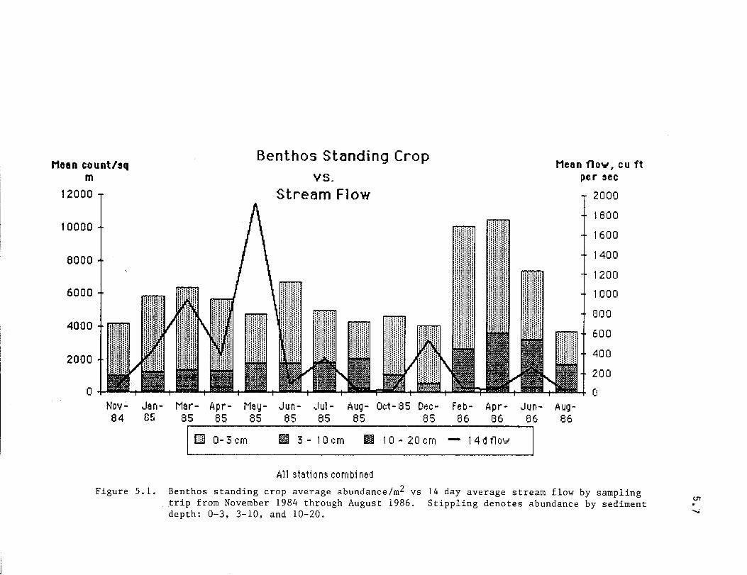
Mean count/sq m

12000

10000

8000

6000

4000

2000

o

Figure 5.1.

Benthos Standing Crop vs.

Stream Flow

Mar- Apr- May- Aug- Oc:t- 85 Dec-85 85 85 85 85 85

mm 0 ~ u.l.UI - ~ I~m ml 3 - 1 0 I~rn III 1 I) - 20 ern - 14d tl,)\0,1

All stations combi ned

86

Mean flo .... , cu ft per sec

2000

1800

1600

1400

1200

1000

800

600

400

200

o

Benthos standing crop average abundance/m2 vs trip from November 1984 through August 1986. depth: 0-3, 3-10, and 10-20.

14 day average stream flow by sampling Stippling denotes abundance by sediment

tTl

......

Mean. mg/sq m

100000

90000

80000

70000

60000

50000

40000

30000

20000

10000

a

Figure 5.2. Benthic Biomass vs

Stream Flow Mean flo ...... cu

ft per sec 2000

1800

1600

1400

1200

1000

800

600

400

200

o Nov- Jan- Mar- Apr- May- Jun- Jul- Aug- Oct-8S Dee- Feb- Apr- Jun- Aug-8485 85 85 85 85 85 85 85 86 86 86 86

\liiill 0 - :3 em II 3 - 10 em III 1 0 - 20 em - 14 d flow I All stations combi ned

Figure 5.2. Benthos biomass vs 14 day average streamflow by sampling trip fr~m November 1984 through August 1986. Stippling denotes biomass wet weight (mg/m ) by sediment depth: 0-3, 3-10, and 10-20 em.

c.n

00

Mean. Figure 5.3.

Mean flo .... cu ft mo/sq m

Moll usc bj omass vs. per sec

90000

80000

70000

60000

50000

40000

30000

20000

10000

0

Stream Flow 2000

1800

1600

1400

1200

1000

800

600

400

200

0 Nov- Jen- Mer- Apr- Mey- Jun- Jul- Aug- Oct- 85 Dec- Feb- Apr- Jun- Aug-84 85 85 85 85 85 85 85 85 86 86 86 86

I !ilil 0- 3 em 11m 3 - 10 em III! 10 - 20 em - 14 d nO'vl I All steti 0 ns co m bi ned

Figure 5.3. Mollusc biomass ~s 14 day average streamflow by sampling trip. Stippling denotes wet weight (mg/m ) by sediment depth: 0-3, 3-10, and 10-20 em.

.<J1 Co

MeaD, mg/sq m

Figure 5.4. Benthic biomass - Mollusc biomass vs.

MeaD flo .... , cu ft per sec

12000

10000

8000

6000

4000

2000

o

Stream Flow

Nov- Jen- Mar- Apr- Mey- Jun- Jul- Aug- Oct-8s Dec- Feb- Apr- ,Jun- Aug-84 85 85 85 85 85 85 85 85 86 86 86 86

I III] 0 - 3 c m 11m 3 - 1 0 em Ill! 1 0 - 20 em - 1 4 d 11 0'1/ I

A 11 stat; 0 os co m bi ned

2000

1800

1600

1400

1200

1000

800

600

400

200

o

Fig. 5.4. Benthos biomass minus mollusc biomass vs 14 day average streamflow by sampling trip from November 1984 through August 1986. Stippling denotes biomass wet weight (mg/m2): by sediment depth: 0-3, 3-10, and 10-20 cm.

U'1

..... o

Mean countl sq m

2500

2000

1500

1000

500

o I wo,;,;,:.! I

Nov-84

Jen-85

Figure 5.5.

Figure 5.5. Chlronomld larvae VS.

Stream Flow

Mer- Apr- Mey- Jun- Jul-85 Aug- Oct-8S Dec- Feb- Apr- Jun-85 85 85 85 85 85 86 86 86

I [l] 0- 3 em III 3 - 10 ,;m II1II 10 - 20 em - 14 d flOIN' I All stations combi ned

Mean flo .... cu ft

Aug-86

per sec

2000

1800

1600

1400

1200

1000

800

600

400

200

o

Chironomid average abundance/m2 vs November 1984 through August 1986. 0-3, 3-10, and 10-20 em.

14 day average streamflow by sampling trip from Stippling denotes abundance by sediment depth:

c.n

...... ......

Mean count/ sq m

4000

3500

3000

2500

2000

1500

1000

500

o Nov;. Jen-84 85

Figure 5.6.

Figure 5.6. Streb I ospi 0 benedict i vs.

Stream Flow

Mer- Apr- May- Jun- Jul- 85 Aug- Oct- 85 Dec- Feb- Apr- Jun-85 85 85 85 85 85 86 86 86

Ifill) 0 - 3 em 1m 3 - 1 0 emil 1 0 - 20 em - 1 4 d 11 oW' I

All stations comb; ned

Mean 00 ..... , cu ft per sec

Aug-86

2000

1800

1600

1400

1200

1000

800

600

400

200

o

Streblospio benedicti average abundance/m2 vs 14 day average streamflow by sampling trip from November 1984 through August 1986. Stippling denotes abundance by sediment depth: 0-3, 3-10, and 10-20 cm.

U1

'"" N

Figure 5.7. Mean countl 'q m

Medi omast is cal i torni ensi s

vs. Mean flo .... , eu ft

per ,ee

4500

4000

3500

3000

2500

2000

1500

1000

500

o Nov- Jen-84 85

Stream Flow

Mer- Apr- Mey- Jun- Jul- 85 Aug- Oct- 85 Dec-85 85 85 85 85 85

i

Feb-86

Apr- Jun-86 86

ITIIl 0- 3 em III 3 - 10 ern III 10 - 20 em - 14 d flo",.

All stations combi ned

Aug-86

2000

1800

1600

1400

1200

1000

800

600

400

200

o

Figure 5.7. !1ediomastis californiensis average abundance 1m2 vs 14 day average streamflow by sampling trip from November 1984 through August 1986. Stippling denotes abundance by sediment depth: 0-3, 3-10, and 10-20 cm.

U'I

...... 'w

Figure 5.B. Mean countl sq m

Mulinia lateralis

vs. Mean flo .... cu ft

per sec

500

450

400

350

300

250

200

150

100

50

Stream Flow 2000

1800

1600

1400

1200

1000

800

600

400

200

o I' lit'; ~ I 0

Nov- Jen-84 85

Mer- Apr- Mey- Jun- Jul- 85 Aug- Oct- 85 Dec- Feb- Apr- Jun-85 85 85 85 85 85 86 86 86

I !Ill 0-3 em r.tIB 3 - 10 em II1II 10- 20 em - 14d flo,." I All stations cClmbi ned

Aug-86

Figure 5.8. f.fulinia lateY'alis average abundance/m2 vs 14 day average streamflow by sampling trip from November 1984 through August 1986. Stippling denotes abundance by sediment depth: 0-3, 3-10, and 10-20 cm.

(Jl

..... ~

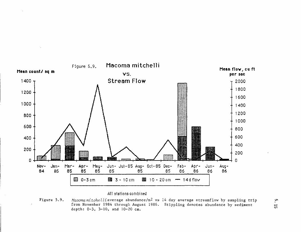
Mean count/ sq m

1400

1200

1000

800

600

400

200

o Nov-84

Jen-85

Figure 5.9.

Figure 5.9. Macoma mitchelli VS.

Stream Flow

Mer- Apr- May- Jun- Jul- 85 Aug- Od- 85 Dee- feb- Apr- Jun-85 85 85 85 85 85 86 86 86

IIlITI 0- 3 em WJ 3 - 10 ern III 10 - 20 ern - 14 d flo"" I

Mean flo ... I CU ft

Aug-86

per sec

2000

1800

1600

1400

1200

1000

800

600

400

200

o

All ststi 0 ns co rn bi ned Macomamitchelliaverage abundance/m2 vs from November 1984 through August 1986. depth: 0-3, 3-10, and 10-20 cm.

14 day average streamflow by sampling trip Stippling denotes abundance by sediment

CJl

...... CJl

5.16

Table 5.1. Lavaca Bay Macrobenthos Species List, November 1984-August 1986

PHYLUM PLATYHELMINTHES Flatworms (unidentified)

PHYLUM NEMERTINIA (=Rynchocoela)

PHYLUM MOLLUSCA Class Gastropoda

Class Pelicypoda

PHYLUM ANNELIDA Class Polychaeta

Nemerteans (unidentified)

Pyramidell idae Odostomia laevigata Odostomia cf. gibbosa

Acteonidae Acteon punctostriatus

Solenidae Ensis minor

Tellinidae Macoma mitchelli Macoma tenta macoma sp.

Mactridae Mulinia lateralis Rang;a cuneata

Solecurtidae Congeria leucophaeta Tagelus plebius

Phyllodicidae Eteone heteropoda

Pi 1 argi ldae Sigambra tentaculata Anclstrosyllls jonesi Loandalia americana Parandal ;a sp •. Pilargidae unidentified

Hes i oni dae Gyptis vittata

Neri idae Nereid juvenile Laeoneris culveri Neanthes succ;nia

Glyceridae Gl ycera capitata

Spionidae Polydora socialis Streblospio benedicti Scolelepis texana

Cossuridae Cossura delta

Orbinidae Haploscloplos foliosus

Capitell idae Capitella capitata Mediomastus californiensis Heteromastus fllifonmls

Ampharetidae Hobsonia florida

Class Oligochaeta Oligochaetes (unidentified)

Cl ass Hi rud i nea Leeches (unidentified)

PHYLUM ARTHROPODA

Class Crustacea Subclass Copepoda

Order Cyclopoida Cyclopidae

Hemicyclops sp.

L i chomol gidae Cyclopoid copepod (commensal)

Subclass Malacostraca Order Mys i dacea

Order Cumacea

Mysidopsis sp. juvenile Mysidopsis almrya

Cyclaspis varians Cumacean unidentified

Order Tanaidacea Tanaidae

Leptoche 1 i a rapax

Class Insecta

Order Isopoda Idoteidae

Edotea montosa

Order Amphi poda Ampeliscidae

Ampel isca abdita

Oedicerotidae Monoculodes nyei

Corophiidae Corophium louisianum

Order Oecapoda suborder Reptantia Callianassidae

Callianassa juvenile Callianassa jamalcense Callianassa latispina

Portunidae Callinectes sapidus

Insect larva (unidentified) Order Oi ptera

Chi ronomidae Chironomid larva Chironomid pupa

.5.18

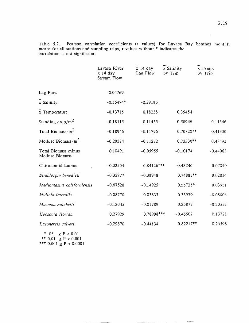
5.19

Table 5.2. Pearson correlation coefficients (r values) for Lavaca Bay benthos monthly means for all stations and sampling trips, r values without * indicates the correlation is not significant.

Lag Flow

-x Salinity

-x Temperature

Standing crop/m2

Total Biomass/m2

Mollusc Biomass/m2

Total Biomass minus Mollusc Biomass

Chironomid Larvae

Streblospio benedicti

Mediomastus californiensis

Mulinia latera lis

Macoma mitchelli

Hobsonia florida

Laeonereis cui veri

* .05 s P < 0.01 ** 0.01 :0. P < 0.001

*** 0.001 :0. P < 0.0001

Lavaca River x 14 day Stream Flow

-0.04769

-0.55474*

-0.13715

-0.18115

-0.18946

-0.20574

0.10491

-0.02554

-0.35877

-0.07520

-0.08770

-0.12045

0.27929

-0.29870

-x 14 day Lag Flow

x Salinity by Trip

-0.39186

0.18238 0.35454

0.11435 0.50946

-0.11796 0.70820**

-0.11272 0.73330**

-0.05955 -0.10174

0.84126*** -0.48240

-0.38948 0.74885**

-0.14925 0.55725*

0.03833 0.33979

-0.01789 0.25877

0.78998*** -0.46502

-0.44134 0.82217**

x Temp. by Trip

0.11346

0.41330

0.47492

-0.44063

0.07840

0.02836

0.03951

-0.08005

-0.20552

0.13728

0.26598

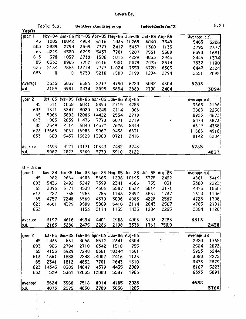
lavaca Bay

Table 5.3. s..atbo •• t.ladi"CJ crop lladivichlab/",-Z 5.20 Totals year 1 Nov-84 Jan-85 Mar-85 Apr-85 May-85 Jun-85 Jul-65 AiIg-65 Average :I.d.

45 1285 10042 4984 6116 1435 10269 6040 3549 5465 3226 603 5889 2794 3549 7777 2417 5437 1360 1133 3795 2377

65 4229 4530 6795 5437 7701 9287 7551 5588 6390 1631 613 378 1057 2718 1586 1813 4229 4833 2945 2445 1394

85 8533 8985 7702 6116 7551 8079 7475 5814 7532 1100 623 5134 7853 13214 7777 11024 . 7550 6720 8305 8447 2324 633 0 0 5739 5210 1588 2190 1284 2794 2351 2095

jAverage 3635 5037 6386 5717 4790 6720 5038 4304 5203 S.d. 3189 3981 3474 2090 3894 2889 2700 2404 3094

year 2 Oct-85 Dec-85 feb-86 Apr-86 Jun-86 Aug-86 Average S.d. 45 1511 1058 6041 5890 2719 4758 3663 2196

603 1511 3247 3020 7248 2114 906 3008 2258 65 5966 5892 12005 14422 12534 2719 8923 4673

613 1963 2039 11476 7778 6871 2719 5474 3873 I 85 3549 2114 6040 14572 7626 5814 6619 4358

623 17668 9061 16988 9967 9438 6871 11666 4516 633 680 5437 15629 13968 10721 2416 8142 6204

Average 4693 4121 10171 10549 7432 3743 6735 S.d. 5987 2822 5269 3730 3910 2122 4837

0- 3 em year 1 Nov-84 Jan-85 Mar-85 Apr-85 May-85 Jun-85 Jul-85 Aug-85 Average S.d.

45 982 9664 4908 5663 1208 10193 3775 2492 4861 3419 603 5436 2492 3247 7399 2341 4606 755 831 3388 2323

'C O,J 3096 3171 4530 4606 5587 8532 5814 3171 4813 1850 613 227 755 1963 755 1133 2492 3851 1737 1614 1106

'-'I:' O,J 4757 7248 6569 4379 3096 4983 4228 2567 4728 1708 623 4681 4379 9589 5889 6418 2114 2643 2567 4785 2701 633 4153 2114 1135 1435 1284 2265 2064 1120

Average 3197 4616 4994 4401 2988 4908 3193 2233 3813 S.d. 2163 3286 2475 2286 2198 3338 1761 750.9 2438

y~r 2 Oct-85 Dec-85 feb-86 Apr-86 Jun-86 Aug-86 • Average S.d . 45 1435 831 3096 5512 2341 4304 2920 1765

603 906 2794 2718 6342 1510 755 2504 2072 65 4153 3929 7248 8381 10344 1661 - 5953 3244

613 1661 1888 7248 .4002 2416 1133 3058 2275 85 2341 1812 4832 7701 2643 1510 3473 2379

623 14345 8305 14647 4379 4455 2669 8167 5223 633 529 5361 12835 12080 5587 1963 6393 5091

Average 3624 3560 7518 6914 4185 ·2028 4638 S.d. 4873 2575 4638 2789 3056 ·1205 3766

L8V8C8 Bay

Table 5.3 (Cont:) 8entbosstandiDgcrop

3-10 cm year 1 Nov-84 Jan- 85 Mar-85 Apr-85 May-85 Jun-85 Jul-85 AUg-85

45 227 227 76 302 227 76 2114 1057 603 302 302 302 378 76 755 529 302

65 906 1208 1661 453 2114 604 1661 2190 613 lSI 302 604 831 604 1586 906 1057

85 3398 1586 1133 1586 4228 2869 2869 2794 623 453 3247 3398 1586 4304 5134 4077 4681 633 1586 1510 453 755 0 378

Average s.d.

year 2 45

603 65

613 85

623 633

Average s.d.

906.2 1145 1251 949.4 1715 1683 1737 1780 1250 1173 1126 595.9 1867 1770 1418 1571

Oet-85 Dee-85 Feb-86 Apr-86 Jun-86 Aug-86 76 151 2869 302 302 378

529 453 302 906 604 lSI 1586 1963 4379 5965 2114 982 302 151 4228 2945 2869 906

1208 302 1208 6418 4681 3851 3247 680 2341 4908 4681 3700

151 0 2794 1586 5134 453

1014 528.6 2589 3290 2912 1489 1134 671.1 1484 2490 1999 1590

10-20 em year 1 Nov-84 Jao-85 Mar-85 Apr-aS May-85 Jun-85 Jul-85 Aug-a5

45 76 151 0 151 0 0 151 0 603 151 0 0 0 0 76 76 0

65 227 151 604 378 0 151 76 227 613 0 0 151 0 76 151 76 151

85 378 151 0 151 227 227 378 453 623 0 227 227 302 302 302 0 1057 633 0 0 0 1586 0 0 0 lSI

Average 118.9 97.14 140.3 366.9 86.43 129.6 108.1 291.3 s.d . 143.8 94.76 224.1 555.7 126.6 113 129.8 371

.

year 2 Oct-85 Dec-85 feb-86 Apr-86 Jun-86 Aug-86 45 0 76 76 76 76 76

603 76 0 0 0 0 0 65 227 0 378 76 76 76

613 0 0 0 831 1586 680 85 0 0 0 453 302 453

623 76 76 0 680 302 302 633 0 76 0 302 0 0

Avereqe 54.14 32.57 64.86 345.4 334.6 226.7 s.d. 84.22 40.62 141 322.9 566.5 261.6

..• 5.21

Average s.d. 538.3 754.4 368.3 213.5 1350 687.5

755.1410.1 2558 1069 3360 1173 780.3 641.9

1410 1356

Average s.d. 679.7 1078 490.8 260.5 2832 1921 1900 1676 2945 2405 3260 1577 1686 1992

1970 1872

Average s.d. 66.13 80.71 37.88 37.08 226.8 204.5 75.63 67.9 245.6 151.1 302.1 331.5 217.1 592.6

167.3 268.1

Avereqe s.d. 63.33 31;03 12.67 31.03 138.8 138.6 516.2 643.4 201.3 227.3 239.3 250.1

63 121

176.4 .307

Lavaca Bay

5.22 Table 5.4. Benthlc blomass

Totals year 1 Nov-84 Jan-85 Mar-85 Apr-85 May-85 Jun-85 Jul-85 Aug-85 Aver-age s.d.

45 6349 10601 1925 2915 7717 3413 3020 687 4578 3522 603 5373 3277 2870 6946 1133 1488 816 506 2801 2243

6S 14783 3775 13567 26727 19337 4093 4402 3904 11324 9283 613 348 2363 30379 6130 3043 27911 2454 3095 9465 12638

85 3254 8623 13492 11975 30834 1[+05 4952 1570 22757 37272 623 3142 17811 55546 36685 46720 9951 28222 3[+05 57720 88796 633 0 (I 36927 33235 48781 19902 8985 34294 22766 17138

Average 4750 6636 22101 17802 22509 24873 7550 43963 18773 s.d. 5006 6142 19709 14048 20043 37636 9468 97642 38309

year 2 Oct-85 Dec-85 feb-86 Apr-86 ,-'un-86 Aug-86 Average s.d. 45 2024 9017 27730 26063 3587 1986 11735 12035

603 1035 959 1948 4138 2159 747 1831 1266 65 2250 33234 12949 1 [+05 81337 34300 45207 40726

613 763 1578 18905 1[+05 3E+05 29679 74385 lE+05 85 1314 1057 46236 1 [+05 1 E+05 2[+05 75457 70215

623 14068 20506 39713 1 [+05 13643 6200 39964 53014 633 816 16482 40555 96745 23496 890 29831 36029

Average 3181 11833 26862 92865 68970 34925 39773 s.d. 4835 12263 16362 56269 90819 61499 57529

0- 3 cm year 1 Nov-84 Jan-85 Mar-85 Apr-85 May-85 Jun-85 Jul-85 Aug-85 Average s.d.

45 1306 2514 1895 2069 1601 3224 1155 498 1783 889.9 603 1344 2205 1435 6463 944 1050 619 317 1797 2118 65 438 2522 6251 3179 17413 3058 3352 1933 4769 5478

613 8 1638 8129 2008 491 8818 1510 664 2908 3565 85 1336 7694 10094 6146 3835 2469 732 672 4122 3597

623 2575 4047 17207 6070 2643 566 21238 35598 11243 12809 633 14058 6584 1963 264 8985 461 5386 5510

Average 1168 3437 8438 4646 4128 2778 5370 5735 4542 s.d. 887.3 2233 5887 2125 5963 2917 7590 13180 6348

year 2 Oct-85 Dec-85 feb-86 Apr-86 Jun-86 Aug-86 Average s.d. 45 355 644 6922 17546 657 1102 4538 6847

603 589 642 1608 2356 287 619 1017 794.6 65 1019 1389 7943 6644 2711 1450 3526 3002

613 559 1434 6455 1993 642 196 1680 2335 85 385 853 26863 4409 914 619 5674 10488

623 2977 8396 27475 2401 1155 914 7220 10290 633 544 4153 24458 54519 1699 649 14337 21717

Average 918.3 2502 14532 12838 1152 792.7 ·5456 s.d . 933.4 2872 11193 19172 820~5 404 10432

.

lavaca Bay

Table 5. 4(Cont.} Benthic biomass

3-10 em year 1 Nov-84 Jan-85 Mar-85 Apr-85 Nay-85 Jun-85 Jul-85 Aug-85

45 4590 914 30 793 6116 189 581 189 603 4021 1072 1435 453 189 166 189 189

65 14322 951 7029 17093 1896 1012 1050 740 613 340 725 16157 4122 2446 1253 649 2242

85 1465 838 3398 5640 3050 31937 4062 196 623 559 4832 30766 446 13877 4115 6946 10230 633 22869 23805 46816 19638 0 4916

Average 4216 1555 11669 7479 10627 8330 1925 2672 S.d. 5259 1609 11835 9284 16564 12513 2604 3754

year 2 Oct-65 Dec-85 feb-86 Apr-86 Jun-86 Aug-86 45 1669 2778 2356 2741 1865 378

603 446 272 340 1782 1835 68 65 1231 1744 5006 77795 76957 15749

613 189 144 12450 40060 80483 748 85 929 151 19373 92563 23911 4825

623 10676 1872 12238 12095 11982 4908 633 272 68 16097 40135 21737 241

Average 2202 1004 9694 38167 31253 3845 S.d. 3775 1105 7212 36045 33559 5667

10-20 em year 1 Nov-84 Jan- 85 Mar-85 Apr-85 May-85 Jun-85 Jul-85 Aug-85

45 453 7173 0 53 0 0 1284 0 603 8 0 0 30 0 272 8 0

65 23 302 287 6455 23 23 0 1231 613 0 0 6093 0 106 17840 295 189

85 453 91 0 189 23949 72948 158 702 623 8 8932 7573 30169 30200 5270 38 2E + 05 633 0 2846 0 0 0 2891 7

Average 157.5 2750 1993 5677 7754 13765 254.7 35556 S.d. 229 4147 3335 11063 13321 26899 466.9 81086

year 2 Oct-85 Dec-85 feb-86 Apr-86 Jun-86 Aug-86 45 0 5595 18452 5776 1065 506

603 0 45 0 0 37 60 65 o 30101 o .22733 1669 17101

613 15 0 o 99449 2E+05 28735 85 0 53 o 31808 79856 2E+05

623 415 10238 o lE+05 506 378 633 0 12261 O· 2091 60 0

Average 61.43 8328 2636 41859 36565 30287 S.d. 156 10856 6974 52271 66918 60551

5.23

Average s.d. 1675 2167

964.3 516.4 5512 6085 3492 5520 6323 11144 8971 10067

19674 16547

6177 9695

Average S.d. 1965 898 790.5 798.3

29747 37263 22346 32379 23625 35186

8962 4457 13092 16212

14361 24358

Average S.d. 1120 2670 39.75 101 1043 2362 3065 6703

12311 27454 37506 78089

5294 11629

8749 31475

Average S.d. 5232 6961 23.67 26.96 11934 13142 50160 71·366 46158 66192 23783 52753

2402 4901

19956 . 43649

.

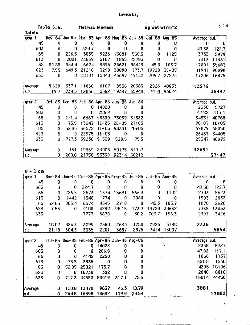
L8V8C&Bay

Table 5.5. HoH usc biomass 5.24 Totals year 1 Nov-84 Jan-<J5 Mar-85 Apr-85 May-85 Jun-85 Jul-85 Aug-85 Average s.d.

45 j J 0 0 0 0 0 0 0 0 0 603 0 0 324.7 0 0 0 0 0 40.58 122.7

65 0 226.5 3035 9226 15681 566.3 0 1125 3733 5979 613 0 2001 23669 5167 1865 25783 0 0 7313 11331

85 52.85 883.4 6674 9596 26621 98429 45.3 105.7 17801 35683 623 7.55 649.3 21216 3299 38890 173.7 19728 3E+05 41941 90890 '-;C-0 ... ,) O 0 28101 15440 46697 19132 709.7 27573 17206 16475

Average 6.629 537.1 11860 6107 18536 20583 2926 40053 12576 S.d. 19.7 734.5 12036 5662 19347 35948 7414 93824 36497

year 2 Oct-85 Dec- 85 feb- 86 Apr-86 Jun- 86 Aug- 86 Average S.d. 45 0 0 0 14028 0 0 2338 5727

603 0 0 0 286.9 0 0 47.82 117.1 -c t·" 0 211.4 6667 93809 75039 31582 34551 40768

613 0 75.5 13643 1E+05 2E+05 27165 70167 1[+05 65 0 52.85 36572 lE+05 96301 2E+05 69879 68050

623 0 0 22975 1 E+05 0 0 26487 54405 633 0 717.3 59230 91529 528.5 75.5 25347 40079

IAverage a 151 19869 84003 60175 31947 32691 S.d. a 260.8 21758 55390 92314 60212 57147

0- 3 em year 1 Nov-84 Jan-85 Mar-85 Apr-85 May-85 Jun-85 Jul- 85 Aug- 85 Average S.d.

45 0 0 0 0 0 0 0 0 0 0 603 0 0 324.7 0 0 0 0 0 40.58 122.7

65 0 226.5 2673 1374 15681 566.3 0 1102 2703 5623 613 0 1442 1548 1774 0 7980 0 0 1593 2832

85 52.85 883.4 6674 4545 2718 0 45.3 105.7 1878 2626 623 7.55 0 4100 3299 98.15 173.7 19728 34632 7755 13333 633 7777 5670 0 30.2 709.7 196.3 2397 3426

Average 10.07 425.3 3299 2380 2643 1250 2926 5148 2336 S.d. 21.18 604.3 3035 2201 5837 2975 7414 13007 5854

year 2 Oct-85 Dec-85 feb-86 Apr-S6 Jun-86 Aug-86 Average S.d. 45 0 0 0 14028 0 0 2338 5727

603 0 0 0 286.9 0 0 47.82 117.1 65 0 0 4145 2250 0 0 1066 1757

613 0 75.5 3835 0 0 0 651.8 1560 85 0 52.85 25021 173.7 0 0 4208 10196

623 0 0 16738 302 0 0 2840 6810 633 0 717.3 44553 50419 317.1 75.5 16014 24450

Average 0 120.8 13470 9637 45.3 10.79 3661 s~d. 0 264.8 16598 18682 119.9 28.54 11082

Table 5.5 (Cont.) Monusc biomass 5.25

3-10 em year 1 Nov-84 J8n135 Mar-85 Apr-85 May-85 Jun-85 Ju1-65 AUg-85 Average 3~d.

45 0 0 0 0 0 0 0 0 0 0 603 0 0 0 0 0 0 0 0 0 0

65 0 0 362.4 7218 0 0 0 15.1 949.4 2708 613 0 558.7 16029 3413 1865 (I 0 0 2733 5832

85 0 0 0 5051 0 28048 0 0 4137 10454 623 0 649.3 17116 0 9007 0 0 0 3347 6734 633 20325 9770 46697 19102 0 (I 15982 17444

Average 0 201.3 7690 3636 8224 6736 0 2.157 3430 s.d. 0 313.2 9567 3919 17281 11790 0 5.707 8611

year 2 Oct-85 Dec-85 feb-86 Apr-86 Jun-86 Aug-86 AverBge s.d. 45 0 0 0 0 0 0 0 0

603 0 (I 0 0 0 0 0 0 65 (I 52.85 2522 69241 75039 14481 26889 35505

613 0 0 9807 33779 76527 0 20019 30624 85 0 0 11552 88690 19064 0 19884 34613

623 (I 0 6236 6055 0 0 2049 3174 633 0 0 14677 39388 211.4 0 9046 15974

Average 0 7.55 6399 33879 24406 2069 11127 s:d. 0 19.98 5826 35011 35780 5473 23551

t 0-20 em year 1 Nov-54 Jan-85 Mar-55 Apr-85 May-aS JUIl-85 Jul-85 Aug-85 Average s.d.

45 0 0 0 0 0 0 0 0 0 0 603 0 0 0 0 0 0 0 0 0 (I

65 0 0 0 634.2 0 0 0 7.55 80.22 239.2 613 0 0 6093 0 0 17803 0 (I 2987 6739

85 0 0 0 0 23903 70381 0 0 11786 26630 623 (I 0 (I 0 29785 0 o 2E+05 30840 80882 633 0 0 0 0 o 27376 4563 11176

Average 0 0 870.4 90.6 7670 12598 0 34903 7276 s.d. 0 0 2303 239.7 13208 26330 0 80914 31238

year 2 Oct-85 Dec-85 feb-86 Apr-86 Jun-86 Aug-86 Average s.d. 45 0 0 0 0 0 0 0 0

603 0 0 0 0 0 0 0 0 65 0 158.6 o 22318 0 17101 6596 10291

613 0 0 o 99109 2[+05 27165 " 49517 70754 85 0 0 o 30676 79237 2E+05 45787 66035

623 0 0 0 1[+05 0 0 21598 52904 633 0 0 0 1721 0 0 286.9 702.8

Average 0 22.65 0 40487 35723 29668 17684 3.d. 0 59.93 0 52572, 66492 60461 43778

.

l8V1lC8 Bay

Table 5.6. Benthic biorrntss - mollusc biomass JIg wet yt/m6 2

Totals 5.26

year 1 Hov-84 Jen-85 I18r.-85 Apr-85 l18y-85 Jun-85 Jul-85 Aug-85 Average s.d . 45 6349 10601 1925 2915 7717 3413 3020 . 687 4578 3522

603 5373 3277 2545 6946 1133 1488 816 506 2761 2236 65 14783 3549 10532 17501 3656 3527 4402 2779 7591 5494

613 348 362.3 6710 943.2 1759 2128 2454 3095 2225 2072 85 3201 7740 6818 2379 4213 8925 4907 1464 4956 2766

623 3134 17162 34331 33386 7830 9777 8494 12117 15779 11539 633 0 0 8826 17795 2084 770.3 8275 6721 5559 6200

Average 4741 6099 10241 11695 4056 4290 4624 3910 6207 s.d. 5009 6190 11068 11856 2755 3602 2893 4186 6994

year 2 Oct-a5 Dec-85 feb-S6 Apr-86 Jun-S6 Aug-66 Average s.d. 45 2024 9017 23730 12035 3587 1986 8730 8401

603 1035 959 1948 3851 2159 747 1783 1163 65 2250 33023 6282 13363 6298 2718 10656 11657

613 763 1503 5262 6614 6531 2514 4198 3098 65 1314 1004 9664 9241 6360 5867 5578 3740

623 14068 20506 16738 9710 13643 6200 13478 5051 633 816 15765 11325 5216 22968 814.5 9484 8867

Average 3181 11682 10707 8862 8795 2978 7701 S.d. 4835 12177 7454 3407 7219 2223 7435

.

0- 3 em year 1 Nov- 84 Jen-85 I18r- 85 Apr- 85 May- 85 Jun- 85 Jul- 85 Aug- 85 Average S.d.

45 1306 2514 1895 2069 1601 3224 1155 498 1783 889.9 603 1344 2205 1110 6463 944 1050 619 317 1757 2132

65 438 2296 3578 1805 1737 2492 3352 830.7 2066 957.3 613 8 196 6581 233.8 491 837.7 1510 664 1315 2283

85 1283 6811 3420 1601 1117 2469 686.7 566.3 2244 2201 623 2567 4047 13107 2771 2545 392.4 1510 966.2 3488 4359 633 6282 914 1963 233.8 8275 264.7 2989 3440

Average 1158 3011 5139 2265 1485 1528 2444 586.7 2207 s.d. 883.1 2229 4063 2022 688.6 1180 2728 256.3 2398

year 2 Oct-85 Dec-85 feb-86 Apr-86 Jun-86 Aug-86 Average s.d. 45 355 644 2922 3518 657 1102 1533 1342

603 589 642 1608 2069 287 619 969 701.1 65 1019 1389 3798 4394 2711 1450 2460 1403

613 559 1359 2620 1993 642 196 1228 937.5 85 385 800.2 1842 4235 914 619 1466 1445

623 2977 8396 10737 2099 1155 914 4380 4150 633 544 3436 9905 -4100 t382 573.5 3323 3550

. Average 918.3 2381 4776 3201 1107 781.9 2194 s.d. 933.4 2824 3863 1107 793.6 409.5 2431

.

l8V8C6 Bay

Tab 1 e 5. 6. (CondJentbie lIiom~s ... moll use biomass JIg .... et vt/m-2

3-10 em year 1 Nov-84 Jen~5 Mar-85 Apr-85 May-85 Jun-85 Ju1-85 ~ug-85

45 4590 914 30 793 6116 189 581' 189 603 4021 1 072 1435 453 189 166 189 189

65 14322 951 6667 9875 1896 1012 1050· 724.9 613 340 166.3 128.4 709.4 581.2 1253 649 2242

85 1465 838 3398 589.1 3050 3889 4062 196 623 559 4183 13650 446 4870 4115 6946 10230 633 2544 14035 121.3 536.5 0 4916

Average 4216 1354 3979 3843 2403 1594 1925 2670 3.d. 5259 1422 4831 5672 2380 1694 2604 3755

year 2 Oct-85 Dec-85 feb-86 Apr-86 Jun-86 Aug-86 45 1669 2778 2356 2741 1865 378

603 446 272 340 1782 1835 68 65 1231 1691 2484 8554 1918 1268

613 189 144 2643 6281 3956 748 85 929 151 7822 3873 4847 4825

623 10676 1872 6002 6040 11982 4908 633 272 68 1420 746.6 21526 241

Average 2202 996.6 3295 4288 6847 1777 S.d. 3775 1099 2647 2788 7398 2147

10-20 em year 1 Nov-84 Jan-85 Mar-aS Apr-aS May-85 Jun-85 Ju1-85 Aug-85

45 453 7173 0 53 0 0 1284 0 603 8 0 0 30 0 272 8 0

65 23 302 287 5821 23 23 0 1224 613 0 0 0.15 0 687.2 37.1 295 189

85 453 91 0 189 45.7 2567 158 702 623 8 8932 7573 30169 415.3 5270 38 920.8 633 0 2846 0 0 0 1541

Average 157.5 2750 1123 5587 167.3 1167 254.7 653.7 S.d. 229 4147 2846 11058 274.3 2037 466.9 613.2

year 2 Oct-aS Dec-85 feb-86 Apr-86 Jun-86 Aug-86 45 0 5595 18452 5776 1065 506

603 0 45 0 0 37 60 65 o 29942 0 415.2 1669 0

613 15 0 0 340.1 1933 1570 85 0 53 0 1132 618.8 423

623 415 10238 0 1571 506 378 633 0 12261 0 369.6 60 0

Average 61.43 8305 2636 1372 841.2 419.6 sA. 156 10803 6974 2015 746.7 549.9

5.27

Average S.d. 1675 2167

964.3 516.4 4562 3625 758.7 731.9 2186 1678 5625 4386 3692 5406

2747 3677

Average 3.d. 1965 898

790.5 798.3 2858 2829 2327 2458 3741 2824 6913 3765 4046 8577

3234 4114

Average S.d. 1120 2670

39.75 101 962.8 2126 151.1 254.2 525.7 925.7 6666 10567 731.1 1206

1484 4482

Average s.d. 5232 6961 23.67 26.96 5338 12071

643 675.9 371.2 451.7 2185 3980 2115 4973

2273 5750

lavaca Bay 5.28

Table 5. 7. Cbi nnomid luvae I ndividuah/m-2 Totals -year 1 Nw-64 Jan-tl5 Mar-85 Apr-65 May-85 Jun-85 Jul-85 Aug-85 Average 3_d_

45 lSI 5965 3171 3398 830_5 8909 3775 2341 3567 2641 603 755 528_5 377_5 2945 98L5 1812 604 755 1010 924.1

65 226.5 226.5 1208 830.5 6795 1888 679.5 679.5 802.2 528 613 0 75.5 604 0 226.5 1359 906 226.5 424.7 498.6

as 0 0 (I 151 151 (I (I (I :;;' ":"Ie _1.1..> 73.68 623 (I 75.5 75.5 2039 75.5 75_5 0 0 292.6 752.3 633 (I (I (I 528.5 75.5 3(12 75.5 0 I?? 7 '- '-. , 201.8

Average 64.71 981.5 776.6 1413 431.4 2049 862.9 571.6 893_9 s.d. 91.73 2205 1141 1378 386.7 3130 1335 844 1604

year 2 Oct- 85 Dec-85 feb- 86 Apr- 86 .Jun- 66 Aug- 86 Average s.d. 45 0 75.5 4757 377.5 0 4002 1535 2220

603 0 0 0 lSI 0 151 50.33 77.98 65 0 (I 830.5 lSI 0 75.5 1-" -. IO.L 326.2

613 (I 75.5 151 151 151 (I 88.08 74.23 c·c (I 0 0 0 0 0 0 0 u..>

623 0 0 0 151 151 0 50.33 77.98 633 (I 0 0 0 75.5 0 12.58 30.:32

I, 0 21.57 819.7 140.2 53.93 604 2732 r .... ~rRQ~ H\., .. __ -

944\ I ::'.It 0 36.'(;4 1762 126.6 71.81 1499

0- 3 em year 1 Nov-84 Jan-85 11ar-85 Apr-85 May-85 Jun-85 Jul- 85 Aug- 85 A'ferage S.d.

45 151 5889 3096 3171 831 8909 3096 1688 ........ 'Q :':'1- 2718

603 76 529 302 2567 906 1812 453 529 896.6 851.8 65 227 227 906 755 529 1888 660 453 707.8 536.9

613 0 76 604 0 227 906 529 76 302 340 (;5 0 0 (I 151 151 (I 0 (I 37.75 73.68

f,?--~:, 0 76 7' .0 1963 76 76 0 0 233. , 723.8

I 633 (I 453 76 302 76 0 151 184.9

lAve rage 75.5 1133 711.9 1294 399-' 1985 690.3 420.6 647_3 S.d. 95.5 2338 1104 1263 356 3151 1095 684.9 1579

year 2 Oct-85 De.c-85 feb-86 Apr-86 Jun-86 Aug-86 Average s_d_ 45 0 76 2190 378 0 3926 1095 1623

603 0 0 0 151 0 151 50.33 77_98 65 0 0 604 151 0 76 138.4 236

613 0 76 151 151 76 0 755 6753 85 0 0 0 0 0 0 0 0

623 0 0 0 151 151 0 50_33 77_98 633 0 0 0 0 76 (I 12.58 30_82

Average 0 21_57 420.6 1402 43_14 593.2 203_1 s_d_ 0 36.84 810_7 126_6 59-4 1471 683_8

Lavaca Batj

Table 5,7 (Cont) Chironomid larvae I ndividuals/m-Z 5.29

3-10 em year I Nov-84 Jan-85 Mar-85 Apr-85 May-85 Jun-85 Jul-85 AUg-85 Average s.d.

I 45 0 76 76 76 0 0 680 453 169.9 264.6

603 0 0 76 378 0 0 151 227 103.8 143.6 65 0 0 151 76 151 0 0 0 47.19 71.81 1

I 613 0 0 0 0 0 453 302 151 113.3 183.5

I 35 0 0 0 0 0 0 0 0 0 0 623 (I (I (I 76 0 0 0 0 9.438 28.54

I 633 0 76 0 (I (I (I 12.53 30.82

I IAverage 0 12.58 43.14 97.07 21.57 64.71 161.8 118.6 61.11 S.d. 0 30.82 59.4 128.7 57.07 171.2 255.8 173.6 140.4

year 2 Oct-85 Dec-85 Feb- 86 A~lr- 86 .. Iun- S6 AU1J- 86 Average S.d. 45 0 (I 2567 0 0 76 440.4 1042

603 0 0 0 0 0 0 0 0 'C o~, (I 0 227 (I 0 (I 37.75 92.47

613 (I 0 0 0 76 (I 12.58 30.82 85 I] 0 0 0 0 I] I] I]

6~-L~ 0 0 0 0 0 (I 0 0 633 0 0 0 I] 0 0 0 O!

I

IAverage 0 0 399.1 0 10.79 10.79 70.11 S.d. 0 (I 959.7 I) 28.54 28.54 396.5

10-20cm year 1 Nov-84 Jan-85 Mar-85 Apr-85 11ay-85 Jun-85 Jul-85 Aug-S5 Average S.d.

45 0 0 0 151 0 0 0 0 1 S.88 57.07 603 0 (I 0 0 76 0 0 0 9.438 28.54

65 0 0 151 0 0 0 0 227 47.19 94.64 613 I] [I (I I] 0 0 76 0 9.438 28.541

r·c 0 0 (I (I 0 (I 0 0 (I 0 0· .. .1

623 (I 0 0 0 0 0 0 0 0 I]

6- 7 :'J 0 0 0 0 0 0 0 0

Average 0 0 21.S7 21.S7 10.79 0 10.79 32.36 12.58 S.d. 0 0 57.07 57.07 2B.54 0 28.54 85.61 43.38

year 2 Oct-85 Dec-85 Feb-86 Apr-86 Jun-86 Aug-S6 Average S.d. 45 0 0 (I 0 0 (I 0 0

603 0 0 0 0 0 0 0 0 65 0 (I 0 0 0 0 0 0

613 0 0 0 0 0 0 0 0

85 0 0 0 0 0 0 0 0

623 0 0 0 0 0 0 (I 0

633 0 0 0 0 0 0 0 0

Average . 0 0 0 0 0 0 0 S.d. 0 0 0 0 0 0 0

.

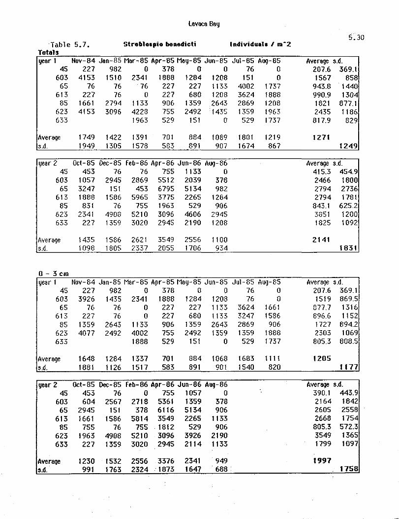
5.30 Table 5.7. Stroble.pie bonedicti

Total $

year 1 Nov-84 Jan-85 Mar-85 Apr-85 May-85 Jun-85 Jul-85 AUg-85 Average s.d. 45 227 982 0 378 0 0 76 0 207.6 369.1

603 4153 1510 2341 1888 1284 1208 151 0 1567 858 65 76 76 76 227 227 1133 4002 1737 943.8 1440

613 227 76 0 227 680 1208 3624 1888 990.9 1304 85 1661 2794 1133 906 1359 2643 2869 1208 1821 877.1

623 4153 3096 4228 755 2492 1435 1359 1963 2435 1186 633 1963 529 151 0 529 1737 817.9 829

Average 1749 1422 1391 701 884 1089 1801 1219 1271 s.d. 1949 1305 1578 583 891 907 1674 867 1249

year 2 Oct-85 Dec-85 feb-86 Apr-86 Jun-86 Aug-86 Average s.d. 45 453 76 76 755 1133 0 415.3 454.9

603 1057 2945 2869 5512 2039 378 2466 1800 65 3247 151 453 6795 5134 982 2794 2736

613 1888 1586 5965 3775 2265 1284 2794 1781 85 831 " .0 755 1963 529 906 843.1 625.2

623 2341 4908 5210 3096 4606 2945 3851 1200 633 227 1359 3020 2945 2190 1208 1825 1092

Average 1435 1586 2621 3549 2556 1100 2141 s.d. 1098 lB05 2337 2055 1706 934 1831

0- 3 ern year 1 Nov-84 Jan-85 Mar-85 Apr-85 May-85 JUrl-85 Jul- 85 Aug- 85 Average s.d.

45 227 982 0 378 0 0 76 0 207.6 369.1 603 3926 1435 2341 1888 1284 1208 76 0 1519 869.5

65 76 76 0 227 227 1133 3624 1661 877.7 1316 613 227 76 0 227 680 1133 3247 1586 896.6 1152

85 1359 2643 1133 906 1359 2643 2869 906 1727 894.2 623 4077 2492 4002 755 2492 1359 1359 1888 2303 1069 633 1888 529 151 0 529 1737 805.3 808.5

Average 1648 1284 1337 701 884 1068 1683 1111 1205 s.d. 1881 1126 1517 583 891 901 1540 820 1177

year 2 Oct-85 Dec-85 feb-86 Apr-86 Jun-86 Aug-86 Average s.d. 45 453 76 0 755 1057 0 390.1 443.9

603 604 2567 2718 5361 1359 378 2164 1842 65 2945 lSI 378 6116 5134 906 2605 2558

613 1661 1586 5814 3549 2265 1133 2668 1754 85 755 76 755 1812 529 906 805.3 572.3

623 1963 4908 5210 3096 3926 2190 3549 1365 633 227 1359 3020 2945 2114 1133 1799 1097

Average 1230 1532 2556 3376 2341 949 1991 s.d. 991 1763 2324 --1873 1647 688 1158

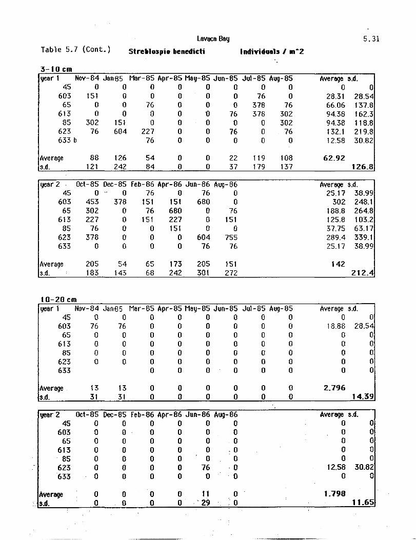
Table 5.7 (Cont.)

3-10 em

Lavaca Bay

Stl"eblospio benedieti

year 1 Nov-84 Jan£5 Mar-85 Apr-85 May-85 Jun-85 Jul-85 Aug-85 45 0 0 0 0 0 0 0 0

603 151 0 0 0 0 0 76 0 65 0 0 76 0 0 (I 378 76

613 (I 0 0 0 0 76 378 302 85 302 151 0 0 0 0 0 302

623 76 604 227 0 0 76 0 76 633 b 76 0 0 0 0 0

Average 88 126 54 0 0 22 119 108 s.d. 121 242 84 0 0 37 179 137

year 2 Oct-85 Dec-85 feb-86 Apr-86 Jun-86 Aug-86 45 o .. 0 76 0 76 0

603 453 378 151 151 680 0 65 302 (I 76 680 0 76

613 227 0 151 227 0 151 85 76 0 0 151 0 0

623 378 0 0 0 604 755 633 0 (I 0 0 76 76

Average 205 54 65 173 205 151 s.d. 183 143 68 242 301 272

10-20 em year 1 Nov-84 Jan£5 Mar-85 Apr-85 May-85 Jun-85 Jul- 85 Aug- 85

45 0 0 0 0 0 0 0 0 603 76 76 (I 0 0 (I 0 0

65 0 0 0 0 0 0 0 (I

613 0 0 0 0 0 0 (I (I

85 0 0 0 0 0 0 (I 0 623 0 0 0 0 0 0 0 0 633 0 0 0 0 0 0

Average 13 13 0 0 0 0 0 0 s.d. 31 31 0 0 0 0 0 0

year 2 Oct-85 Dec-8S Feb-86 Apr-86 Jun-86 Aug-86 45 0 0 0 0 0 0

603 0 0 0 0 0 0 65 0 0 0 0 0 0

613 0 0 0 0 0 .0 85 0 0 0 0

. 0 0

623 0 0 0 0 76 ·0 633 0 0 0 0 0 ·0

Average 0 0 0 0 t1 0 . s.d. 0 0 0 0 ··29 ~ 0

.

5.31

Average s.d. o 0

28.31 28.54 66.06 137.8 94.38 162.3 94.38 118.8 132.1 219.8 12.58 30.82

62.92 126.8

Average s.d. 25.17 38.99

302 248.1 188.8 264.8 125.8 103.2 37.75 63.17 289.4 339.1 25.17 38.99

142 212.4

Average s.d. 0 0

18.88 28.54 0 0 (I (I

0 0 0 0 (I (I

2.796 14.39

Average s.d. 0 0 0 0 0 0 0 0 0 0

12.58 30.82 0 0

1.798 11.65

5.32 Table 5.B.

Totals I)e8r 1 Nov-84 Jan-85 Mar-85 Apr-85 May-85 Jun-85 Jul-85 Aug-85 Average :I.d.

45 76 76 0 76 378 0 0 0 75.s 137.8 603 604 0 0 0 76 76 76 0 103.8 40.36 65 2341 1963 2794 2794 2643 2567 1359 1435 2237 630

613 0 680 151 529 378 453 76 151 302 225.9 85 6267 4077 5587 4077 5210 3851 4153 3700 4615 721.5

623 680 3096 4530 2039 5059 4077 3775 4530 3473 1024 633 1133 680 227 982 0 76 515.9 483.2

Average 1661 1648 2028 1456 1995 1715 1348 1413 1658 S.d. 2409 1666 2312 1554 2316 1762 1654 1929 1877

year 2 Oct-85 Dec-85 feb-86 Apr-86 Jun-86 Aug-86 Average S.d. 45 151 151 151 755 453 0 276.8 277.1

603 0 0 76 529 302 0 151 218.8 65 680 4757 6644 4379 6191 604 3876 2645

613 982 227 1812 1963 1586 906 1246 659.5 85 2265 1812 755 9287 5814 4379 4052 3152

623 2265 3171 7852 4832 3775 3096 4165 1997 633 151 2567 7097 8532 6267 831 4241 3517

Average 928 1812 3484 4325 3484 1402 2572 S.d. 975 1809 3538 3543 2693 1677 2713

0- 3 em year 1 Nov-84 Jan-85 Mar-85 Apr-85 May-85 Jun-85 Jul-85 Aug-85 Average S.d.

45 76 76 0 0 378 0 0 0 66.06 140.8 603 529 0 0 0 76 0 76 0 84.94 36.84

65 2039 1057 2190 2643 2492 2416 680 378 1737 954.9 613 0 453 151 151 0 0 0 0 94.38 168

85 2945 2716 4530 2567 1057 1284 1057 1208 2171 1299 623 302 755 2265 680 1566 76 680 151 811.6 784.3 633 529 453 227 453 0 76 289.4 221

Average 982 843 1381 928 831 604 356 259 767.6 S.d. 1218 1002 1703 1172 932 926 440 440 t038

year 2 Oct-85 Dec-85 feb-66 Apr-66 Jun-86 Aug-86 Average s.d. 45 151 151 151 660 453 0 264.3 251.5

603 0 0 0 376 151 0 88.08 154.1 65 0 3020 4226 378 4757 76 2076 2187

613 982 151 378 227 0 0 289.4 368;1 85 1208 1510 151 4606 1661 302 1573 1611

623 76 2492 5965 604 302 302 1623 2303 633 151 2567 5059 7550 2416 529 3045 2617

Average 367 1413: 2276 2060 1391 173 1280 s.d. 505 1306 2676· 2677 1731 208 1903

lavaca Bay 5 3 . 3 Table 5.8 (Cont.) Hediomastis califoronicnsis Individuals/m

A

2

3-10 em year 1 Nov-84 Jan~5 Mar-8S Apr-8S May-8S Jun-8S Jul-8S AIl9-85

45 0 0 0 76 0 0 0 0 603 0 0 0 0 0 76 0 0

65 302 906 378 151 151 151 604 1057 613 0 227 0 378 302 453 76 151

85 3020 1359 982 1510 4077 2492 2718 2190 623 378 2190 2265 1284 3247 3700 3096 3926 633 604 227 0 529 0 0

Average 617 780 604 518 11 11 1057 928 1046 s.d. 1189 879 821 616 1762 1448 1373 1510

year 2 Oct-85 Dec-85 feb-86 Apr-86 JUfl-86 Aug-86 45 0 0 0 76 0 0

603 0 0 76 151 151 0 65 680 1661 2416 3851 1435 529

613 0 76 1435 1661 906 378 85 1057 302 604 4681 4077 3700

623 2190 680 1888 4228 3398 2492 633 0 0 2039 906 3851 302

Average 561 7'00 .JULI 1208 2222 1974 1057

s.d. 834 614 981 1986 1762 1448

10-20cm year 1 Nov- 84 Jan-85 Mar- 85 Apr- 85 May- 85 JUfl- 85 Jul- 85 AIl9- 85

45 0 0 0 0 0 0 0 0 603 76 0 0 0 0 0 0 0

65 0 0 227 0 0 0 76 0 613 0 0 0 0 76 0 0 0

85 302 0 76 0 76 76 378 302 623 0 151 0 76 227 302 0 453 633 0 0 0 0 0 0

Average 63 25 43 11 54 54 65 108 s.d. 121 62 86 29 84 113 141 189

year 2 Oct-85 Dec-85 feb-86 Apr-86 Jun-86 Aug-86 45 0 0 0 0 0 0

603 0 0 0 0 0 0 65 0 76 0 151 0 0

613 0 0 0 76 680 529 85 0 0 0 0 76 378

623 0 0 0 0 76 302 633 0 0 0 76 0 0

Average 0 11 0 43 119 173 SJ[ 0 29 . 0 59 250 225 .

Average s.d. 9.438 28.54 9.438 28.54 462.4 379.7 198.2 163.1 • 2293 1044 2510 941.7 226.5 278.4

637.5 1198

Average s.d. 12.58 30.82 62.92 74.23 1762 1233

742.4 704.1 2403 1956 2479 1231 1183 1517

1235 1449

Average s.d. 0 0

9.438 0 37.75 85.61 9.438 28.54

15 t 149.2 151 167.2

0 0

53.13 109.4

Average s.d. 0 0 0 0

37.75 63.17 213.9 307.3

75.5 151 62.92 121 12.58 30.82

57.52 147.1

Lavaca Bay

Table 5.9. Hob30nia florida I ndividuals1m A 2 ,- "") ~

.. 5~ 34

3-10 em year 1 Nov-84 Jan-85 Mar-55 Apr-55 May-55 Jun-55 Jul-55 A·ug-55 Average s.d.

45 0 0 0 0 0 0 453 0 56.63 171.2 603 0 0 0 0 0 0 0 0 0 0

65 0 0 0 0 76 0 0 0 9.438 28.54 613 0 (I 0 0 0 (I 0 (I (I (I

85 0 (I 0 0 0 0 0 0 0 0 623 0 (I 76 0 151 76 0 0 37.75 59.4 633 0 0 (j (I 0 0 0 (I

Average 0 (I 1 1 0 32 11 65 0 15.38 s.d. 0 (I 29 (I eQ

..J, ?Q L, 171 0 66.21

year 2 Oct-85 Dec-85 feb-S6 Apr-S6 Jun-S6 Aug-S6 Average s.d. 45 0 0 (I 0 (1 (I (I (I

603 a (I a 76 (I (I 12.58 30.82 65 0 0 (I (I (I (I (I (I

613 (I (I (I 0 0 (I (I 0 85 0 0 0 0 0 0 0 0

623 0 0 76 0 0 0 i 2.58 30.32 633 (I (I (I 0 0 (I 0 0

Average (I (I 1 1 11 (I (I 3.595 s.d. a (I 29 29 (I 0 16.27

10-20 em year 1 Nov-04 Jan-85 Mar-oS Apr-85 May-85 . .Jun-85 JuJ- 85 Aug- 85 Average s.d.

45 0 (I 0 0 0 0 0 0 0 0 603 (I (I (I (I (I 0 (I 0 (I (I

65 (I 0 0 (I 0 (I (I (I (I (I

613 0 (I 0 (I 0 0 0 (I (I (I oc 0 0 0 0 (I (I 0 (I (I (I <-, ,J

623 0 0 0 (I (I (I 0 (I 0 0 633 0 0 0 0 0 0 0 0

Average 0 0 0 0 0 0 0 0 0 s.d. 0 0 0 0 0 0 0 0 0

year 2 Oct-55 Dec-85 feb- 86 Apr- 86 Jun- 86 Aug- 86 Average s.d. 45 0 (I 0 0 0 0 0 0

603 0 0 0 0 0 0 0 0 65 0 0 0 0 0 0 0 0

613 0 0 0 0 0 0 0 0 85 0 0 0 0 0 0 0 0

623 0 0 0 '0 0 0 0 0 633 0 0 0 0 0 0 0 0

Average 0 0 0 0 0 0 0 s.d. 0 . 0 0 0 0 ·0 0

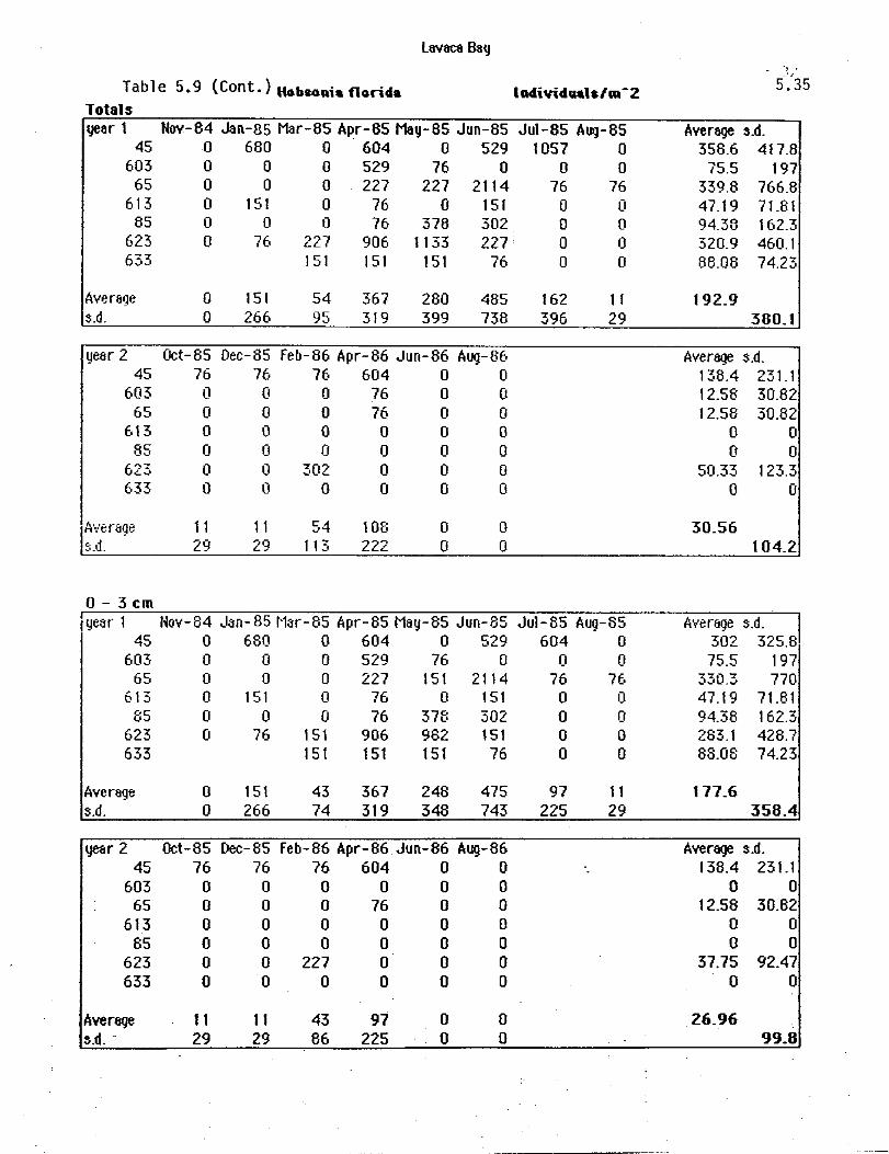
Table 5.9 (Cont.) HobsoRi.f1onu. I ruiividu1&/m-2 Totals year 1 Nov-84 Jan-B5 Mar-85 Apr-85 May-85 Jun-85 Jut-85 Aug-85

45 0 680 0 604 0 529 1057 0 603 0 0 0 529 76 0 0 0

65 0 0 0 227 227 2114 76 76 613 0 151 0 76 0 151 0 (I

85 0 0 0 76 378 302 0 0 623 0 76 227 906 1133 227 0 0 633 151 151 151 76 0 0

Avera'Je 0 151 54 367 280 485 162 1 1 s.d. 0 266 95 319 399 738 396 29

year 2 Oct-85 Dec-aS feb-86 Apr-86 Jun-86 Aug-86 45 76 76 76 604 0 0

603 0 0 0 76 0 (I

65 (I (I 0 76 0 0 613 0 0 0 0 0 0

85 0 (I (I 0 0 0 6'>7 t....J 0 0 302 0 0 (I

633 0 0 0 0 0 0

Average 11 11 54 108 0 0 s.d. 29 29 113 222 0 0

0- 3 em f year 1 Nov-54 ,Jan-85 1'1ar-85 Apr-55 11ay-55 Jun-85 Jut-55 Aug-85

45 0 680 0 604 0 529 604 0 603 0 (I 0 529 76 0 0 0

65 0 0 0 227 151 2114 76 76 613 0 151 (I 76 0 151 0 I)

B5 0 0 0 76 37B 302 0 0 623 0 76 151 906 982 151 0 0 633 151 151 151 76 0 0

Average 0 151 43 367 248 475 97 11 S.d. 0 266 74 319 348 743 225 29

year 2 Oct-65 Dec-85 feb-86 Apr-86 Jun-86 Aug-86 45 76 76 76 604 0 0

603 0 0 0 0 0 0 65 0 0 0 76 0 0

613 0 0 0 0 0 0 85 0 0 0 0 0 0

623 0 0 227 0 0 0 633 0 0 0 0 0 0

Avenige 11 I I 43 97 0 0 3.d .. 29 29 86 225 0 0

, . "

5.35

Average 3.d. 358.6 417.8

75.5 197 339.8 766.8 47.19 71.81 94.38 162.3 320.9 460.1 88.08 74.23

192.9 380.1

Average s.d. 138.4 231.1 12.56 30.82 12.58 30.82

(I 0 0 0

50.33 123.3 0 0

30.56 104.2

Average s.d. 302 325.8 75.5 197

330.3 770 47.19 71.81 94.38 162.3 283.1 428.7 88.08 74.23

177.6 358.4

Average 3.d. 138.4 231.1

0 0 12.58 30.82

0 0 0 0

37.75 92.47 0 0

.

26.96 99.8

Lavaca Bay

·5.36 Table 5.10. lHOMe-eis culveri I Adividu.1s/m-2

Totals year 1 Nov- 64 Janil5 ~r-65 Apr-85 May-85 Jun-65 JuJ-85 Aag-85 Average s.d.

45 76 151 0 0 76 76 0 0 47.19 59.4 603 76 0 0 0 0 0 0 0 9.438 0

65 0 0 76 76 0 0 0 76 28.31 40.36 613 76 0 0 (I 0 0 (I 0 9.438 (I

35 76 0 0 0 (I 0 0 76 18.S8 28.54 623 0 151 76 227 0 0 680 453 198.2 254.2 633 0 0 227 (I 76 378 113.3 156.6

Average SO 50 22 43 43 11 lOS 140 58.72 s.d. 39 78 37 86 86 29 254 192 125.9

year 2 Oct-85 Dec-85 feb-86 Apr-86 Jun-86 Aug-86 Average s.d. 45 76 151 227 1737 302 151 440.4 639.6

603 0 0 0 0 0 0 0 0 65 76 0 0 378 0 0 75.5 151

613 0 0 76 0 227 0 50.33 91.44 85 I) 0 76 0 0 0 12.58 30.82

623 453 151 0 0 151 151 151 165.4 --" \),j" 76 227 0 0 (I 0 50.33 91.44

I Average Q7 -, 76 54 302 97 43 111.5 s.d. 161 97 84 648 129 74 280.6

0- 3 em year 1 No'y'- 84 Janil5 liar-65 Apr-85 tiay-85 Jun-S5 Jul- 85 Aug- 85 Average s.d.

45 76 76 0 0 0 0 0 0 18.88 28.54 603 0 0 (I 0 0 0 (I I) (I (I

65 (I (I (I (I (I (I 0 0 (I 0 613 (I 0 0 0 0 (I 0 0 0 0

85 (I 0 (I 0 0 (I (I 76 9.433 23.54 623 (I 0 76 0 0 0 302 302 84.94 142.7 633 0 0 227 (I 76 227 88.08 111.1

Average 13 13 " 0 32 0 54 86 26.56 s.d. 31 31 29 0 86 (I 113 127 72.09

year 2 Oct-85 Dec-85 Feb-86 Apr-86 Jun-86 Aug-86 Average s.d. 45 76 0 151 1510 151 0 314.6 589.5

603 0 0 0 .0 0 0 0 0 65 76 0 0 227 0 0 50.33 91.44

613 0 0 0 0 0 0 0 0 85. 0 0 0 0 0 0 0 0

623 76 76 0 0 76 0 37.75 41.35 633 76 151 0 0 0 0 37.75 63.17

Average 43 32 22 248 32 0 62.92 s.d. 40 59 57 563 59 0 235.2

L8V8C8 Bay

Table 5.10 (Cont.) Leeoner-ci~ eulvcri Individuals/mAZ

3-10 em . year 1 Nov-84 Jan- 85 Mar-8S Apr-8S May-8S Jun-8S Jul-8S Aug-8S

45 0 0 0 0 76 76 0 0 603 76 0 0 0 0 0 0 0

65 0 0 76 76 0 0 0 76 613 76 0 0 0 0 0 0 0

85 0 0 0 0 0 0 0 0 623 0 76 0 151 0 0 378 76 633 0 0 0 0 0 76

Average 25 13 11 32 1 1 1 1 54 32 s.d. 39 31 29 59 29 29 143 40

year 2 Oct-65 Dec-65 feb-66 Apr-66 Jun-66 Aug-86 45 0 76 0 151 76 76

603 0 0 0 0 0 0 65 0 0 0 151 0 0

613 0 0 76 0 0 0 85 0 0 76 0 0 0

623 302 0 0 0 0 151 633 0 0 0 0 0 0

Average 43 1 1 22 43 1 1 32 s.d. 114 29 37 74 29 59

to-20cm year 1 Nov-84 Jan-85 Mar-85 Apr-6S May-6S Jun-6S Jul-8S Aug-8S

45 0 76 0 0 0 0 0 0 603 0 0 0 0 0 0 0 0

65 0 0 0 0 0 0 0 0 613 0 0 0 0 0 0 0 0

8S 76 0 0 0 0 0 0 0 623 0 76 0 76 0 0 0 76 633 0 0 0 0 0 76

Average 13 25 0 11 0 0 0 22 S.d. 31 39 0 29 0 0 0 37

year 2 Oct-65 Dec-8S feb-86 Apr-86 Jun-86 Aug-86 45 0 76 76 76 76 76

603 0 0 0 0 0 0 65 0 0 0 0 0 0

613 0 0 0 0 227 0 85 0 0 0 0 0 0

623 76 76 0 0 76 0 633 0 76 0 0 0 0

Average 1 1 32 11 1 1 54 11 s.d. 29 40 29 29 84 29

5.37

Average s.d. 18.86 36.84 9.438 0 26.31 40.36 9.436 0

o 0 84.94 135.9 12.58 30.82

60.16

Average s.d. 62.92 56.83

o 0 25.17 61.65 12.58 30.82 12.58 30.82 75.5 126.3

o 0

26.96 61.99

Average S.d. 9.438 26.54

o 0 o 0 o 0

9.438 0 28.31 40.36 12.58 30.82

8.389 23.95

Averaqe S.d. 62.92 30.62

o 0 o 0

37.75 :92.47 o 0

37.75 41.3S 12.56 30.62

21.57 45.01

l8V8C8 Bay

Table 5.11. Hulinia latenlis Individuals/m -2 Totals year 1 Nov-84 Jan-85 Mar-85 Apr-85 May-85 Jun-85 Ju1-85 AiIg-85

45 603

65 613

85 623 633

Average s.d.

year 2 45

603 65

613 85

623 633

Average s.d.

0- 3 em year 1

45 603

65 613

85 623 633

Average s.d.

year 2 45

603 65

613 85

623 633

Average s.d.

0 0 0 0 0 0

o o

Oct-85 0 0 0 0 0 0

76

1 1 29

0 0

76 0

227 0

50 91

0 0

76 76

151 227 151

97 84

0 0

151 0

378 0 0

76 145

0 0

227 0

227 151

0

86 1 1 1

0 0 0 0

302 0

76

54 113

Dec- 85 feb- 86 Apr- 86 Jun- 86 Aug- 86 0 0 378 0 0 0 0 0 0 0

76 151 453 0 0 0 453 0 0 0

76 1284 151 0 0 0 151 76 0 0

227 1359 1208 0 (I

54 485 324 (I 0 84 591 429 0 [I

Nov-84 Jan-85 Mar-85 Apr-aS May-aS Jun-85 0 0 0 0 0 0 0 (I (I 0 0 [I

0 76 76 76 227 0 0 0 76 0 0 (I

0 227 151 378 76 302 0 0 227 0 151 0

1St 0 0 76

0 50 97 65 65 54 0 91 84 141 92 113

,

Oct-85 Dec-85 feb-86 Apr-86 Jun-86 Aug-86 0 0 0 378 0 0 0 0 0 0 0 0 0 0 151 453 0 0 0 0 453 0 0 0 0 76 1284 151 0 0 0 0 151 76 0 0

76 227 1359 1208 0 0

11 43 485 324 0 0 29 ·86 591 429 0 0

0 0 0 0 0

76 76

22 37

0 0

76 0 0 0 0

11 29

Jul- 85 Aug- 85 0 0 0 0 0 76 0 0 (I [I

76 0 76 0

22 11 37 29

5.33

Average s.d. 0 0 0 0

75.5 80.71 9.438 28.54 160.4 143.6 56.63 91.73 50.33 61.65

90-41

Average s.d. 62.92 154.1

0 0 113.3 177.1 75.5 184.9

251.7 509.1 37.75 63.17 478.2 631.1

145.6 340.7

Average s.d. 0 0 [I 0

66.06 75.5 9.438 28.54 141.6 147.4 56.63 91.73 50.33 61.65

46.14 86.04

Average s.d. 62.92 154.1

0 0 100.7. 182.9 75.5 184.9

251.7 509.1 37.75 63.17 478.2' 631.1

143.8· 341_3

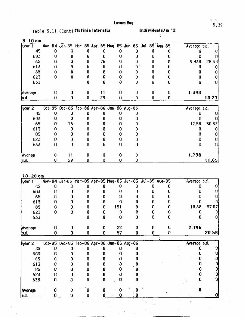
lavaC8 Bay 5.39 Table 5.11 (Cant) Mulinia lateralis Individuals/m &2

3-10 em year 1 Nov-84 Jan-85 Mar-85 Apr-85 May-85 Jun-85 Jul-85 Aug-85 Average s.d.

45 0 0 0 0 0 0 0 0 0 0 603 0 0 0 0 0 0 0 0 0 0

65 0 0 0 76 0 0 0 0 9.438 28.54 613 0 0 0 0 0 0 0 0 0 0

85 0 0 0 0 0 0 0 0 0 0 623 0 0 0 0 0 0 0 0 0 0 633 0 0 0 0 0 0 0 0

Average 0 0 0 11 0 0 0 0 1.398 s.d. 0 0 0 29 0 0 0 0 10.27

year 2 Oct-85 Dec- 85 feb- 86 Apr- 86 Jun- 86 Aug- 86 Average s.d. 45 0 0 0 0 0 0 0 0

603 0 0 0 0 0 0 0 0 65 0 76 0 0 0 0 12.58 30.82

613 0 0 0 0 0 0 0 0 85 0 0 0 0 0 0 0 0

623 0 0 0 0 0 0 0 0 633 0 0 0 0 0 0 0 0

Average 0 11 0 0 0 0 1.798 s.d. 0 29 0 0 0 0 11.65

10-20 em year 1 Nov-84 Jan--85 Mar-85 Apr-85 May-85 Jun-85 Jul-85 Aug-85 Average s.d.

4S 0 0 0 0 0 0 0 0 0 0 603 0 0 0 0 0 0 0 0 0 0

65 0 0 0 0 0 0 0 0 0 0 613 0 0 0 0 0 0 0 0 0 0

85 0 0 0 0 151 0 0 0 18.88 57.07 623 0 0 0 0 0 0 0 0 0 0 633 0 0 0 0 0 0 0 0

Average 0 0 0 0 22 0 0 0 2.796 s.d. 0 0 0 0 57 0 0 0 20.55

year 2 Oct-85 Dec-85 feb-86 Apr-86 Jun-86 Aug-86 Average s.d. 45 0 0 0 0 0 0 0 0

603 0 0 0 0 0 0 0 0 65 0 0 0 0 0 0 0 0

613 0 0 0 0 0 .0 0 0 85 0 0 0 0 - 0 0 0 0

623 0 0 0 0 0 0 0 0 633 0 0 0 0 0 ·0 0 0

Average 0 0 0 0 0 0 0 s.d. 0 0 0 0 0 ~ 0 0

-

Table 5.12 Macoma mitchilli Totals .

year 1 Nov-B4 Jan-8S Mar-BS Apr-8S May-8S Jun-8S 45 0 0 0 0 0 0

603 0 0 0 0 0 0 65 0 76 151 151 0 0

613 0 5291435 378 76 ·151 85 453 982 453 378 76 227

623 76 76 680 15 I 302 0 633 755 151 76 76

Average S.d.

year 2 45

603 65

613 85

623 633

Average S.d.

0- 3 cm year 1

45 603

65 613

85 623 633

Average S.d.

year 2 45

603 65

613 85

623 633

Average s.d.

88 181

OcH35 0 0 0 0 0 0 0

0 0

277 399

Dec-85 0 0 0

76 76

0 604

lOB 222

496 515

173 155

76 107

65 92

feb- 86 Apr- 86 Jun- 86 Aug- 86 0 0 0 0 0 0 0 0

1737 831 378 76 1737 1435 982 76 2265 906 227 0 1057 529 0 0 2794 529 151 76

1370 604 248 32 1076 512 353 40

Nov- 84 Jan- 85 Mar- 85 Apr- 85 May- 85 Jun- 85 0 0 0 0 0 (I

0 0 (I 0 0 0 0 76 (I 76 0 0 0 453 906 227 0 0

453 982 453 302 (I 0 76 0 151 1 5 I (I 0

151 76 (I (I

88 252 237 1 19 (I (I

181 399 336 I 14 0 0

Oct-B5 Dec- 85 feb- 86 Apr- 86 Jun- 86 Aug-'- 86 0 0 0 0 0 0 0 0 0 0 0 0 0 0 1284 0 0 0 0 76 302 0 0 0 0 76 1812 0 0 0 0 0 906 0 0 0 0 604 2265 0 0 76

0 108 938 0 0 t 1 0 222 895 0 0 29

Individuals/m -2

Jul- 85 Ail9- 85 o 0 o 0 o 0 o 0

151 227 76 0 o 76

32 59

43 86

Jul-85 Aug-85 0 (I

0 0 0 0 0 (I

151 227 76 0

0 0

32 32 59 86

5.40

Average s.d. o o o

47.19 320.9 368. I 169.9 188.8

155.2

o 71.81

5 I 1 304.2 242.1 281.5

278.4

Average S.d. 0 0 (I (I

503.3 683.1 717.3 769.6 578.8 894.2 264.3 442.2 692.1 1059

393.7 685.6

Avenige S.d. 0 0 (I (I

18.88 36.84 198.2 346 320.9 340.4 56.63 71.81 37.75 63.17

92.28 206.2

Average S.d. 0 0 0 0

213.9 524 62.92 121 314.6 734.2 : 151 369.9

490,8 900.6

176_2 495_1

Table 5.12 (Cont.) Hacoma mitchilli

3-10 em

lavaca Bay

year I Nov-84 Jan-85 Mar-85 Apr-65 May-85 Jun-85 45 0 0 0 0 0 0

603 0 0 0 0 0 0 65 0 0 151 0 0 0

613 0 76 378 151 76 0 85 0 0 0 76 0 76

623 0 76 529 0 227 0 633 604 76 76 76

Average 0 25 237 43 54 22 S.d. 0 39 263 59 84 37

year 2 Oct-85 Dec-55 Feb-86 Apr-S6 Jun-S6 Aug-86 45 0 0 0 0 0 0

603 0 0 0 0 0 0 65 0 0 453 680 378 76

613 0 0 1435 680 302 0 85 0 0 453 755 151 0

623 0 0 151 151 0 0 633 0 0 529 453 151 0

Average 0 0 431 388 140 11 S.d. 0 0 495 333 154 29

10-20 em year I Nov-84 Jan-8S Mar-85 Apr-85 May-85 Jun-85

45 0 0 0 0 0 0 603 0 0 0 0 0 0

65 0 0 0 76 0 0 613 0 0 151 0 0 151

85 0 0 0 0 76 I 51 623 0 0 0 0 76 0 633 0 0 0 0

Average 0 0 22 11 22 43 S.d. 0 0 57 29 37 74

year 2 Oct-S5 Dec-85 Feb-S6 Apr-S6 Jun-86 Aug-S6 45 0 0 0 0 0 0

603 0 0 0 0 0 0 65 0 0 0 151 0 0

613 0 0 0 755 680 76 . 85 0 0 0 151 76 0 623 0 0 0 378 0 0 633 0 0 0 76 .0 0

Average 0 0 0 216 108 11 s.d. 0 0 ·0 270 254 29

Individuals/m &2

Jul-85 Aug-85 0 0 0 0 0 0 0 0 0 0 0 0 0 0

0 0 0 0

Jul-85 Aug-85 o 0 o 0 o 0 o 0 o 0 o 0 o 76

o o

11 29

5.41

Average s.d. 0 0 0 0

18.86 57.07 84.94 135.9 18.66 36.34 103.8 199.1 138.4 231.1

48.94 122.6

Average S.d. 0 0 0 0

264.3 281.5 402.7 572.3 226.5 313.1 50.33 77.98 188.8 242.3

161.8 299.5

Average S.d. o o

o 28.54 73.68

59.4

o 9.438 37.75 28.31 9.438 12.58

13.98

28.54 30.82

39.01

Average S.d. o 0 o 0

25.17 61.65 251.7 362.6 37.75 63.17 62.92 154.1 12.58 30.82

CHAPTER 6 FINFISH AND SHELLFISH

PURPOSE

6.1

The purpose of this study was to provide data on the utilization of the

Lavaca River delta estuarine zone as a nursery habitat by finfish and selected

macro- in vertebrates. The sampling design was such that both seasonal and

spatial patterns could be investigated.

METHODS

Sampling sites and schedules are described In the Introduction. Finfish

and macro-invertebrates (henceforth referred to as fish except when specific

species are mentioned) were sampled with four types of collecting gear.

Ichthyoplankton were sampled with a 0.5 m diameter conical net made of

505 JIm mesh and a filtering cod end. This net, fitted with a flowmeter to

measure water volume filtered, was towed at the surface for three minutes.

Duplicate samples were taken at each station.

Postlarval and juvenile fish were collected along the shoreline with a

benthic sled and a bag seine. The benthic sled was a 17.8 by 53.3 cm box on

steel runners with a 1800 JIm mesh net attached to one end. This net was

towed 30 m by hand and sampled an area of 12 m2. The seine was 6.1 m long

and 1.8 m high with a 1.8 x 1.8 m bag. The entire seine was made of 2 mm

mesh nylon. This net was pulled along the shoreline for 15 m and sampled an

area of approximately 47 m2. Duplicate sled and seine samples were taken at

each sampling site.

Juvenile fish were collected in open water (i.e. away from shorelines)

with a 3 m otter trawl of 1.9 cm stretched mesh in both the wings and cod

6.2

end and in addition, the cod end was fitted with a liner of .64 cm delta mesh.

This net was towed for 3 minutes at 1200 rpm. Tows were made down-stream

at the river stations and with the wind at all other sites. Trawl samples

were taken in triplicate. Ichthyoplankton and trawl samples, along with

zooplankton samples, were taken at the same sites on the same day. Sled and

seine samples were taken at the same sites on the same day but on different

days from the above mentioned samples. (Sled and seine samples were generally

taken the following day.)

All samples were preserved immediately III 5 percent seawater formalin (l0

percent for trawl samples) and returned to the laboratory for processing. In

the lab, all individuals were counted and up to 50 individuals of each species

were measured (standard length to I mm) and weighed (to the nearest 0.01 g).

When more than 50 individuals of one species were present the total weight

for all individuals was obtained. A voucher collection was established and all

other material was discarded.

The basic analytical tool used for these data was cluster analysis.

Cluster analysis involves the computation of the dissimilarity coefficients

between all possible pairs of entities (i.e., collections) based on the attributes

(i.e., density of each species) of those entities. These coefficients are then

sorted into clusters or groups with high inter-group similarity and the results

are presented in the form of a tree diagram (dendrogram) (see Clifford and

Stevenson 1975, Romberg 1984 for complete discussion of cluster analysis).

The dissimilarity measure used here was the Canberra-Metric (Lance and

Williams 1967a cited by Clifford and Stevenson 1975) which is:

(lin) n E

i=1

x·· - X·k 1J 1

(X·· X·k) 1J = 1

6.3

Where X is the abundance of the ith species at the jth and kth stations

and n = the number of species.

Since this coefficient is the mean of a series of fractions, an

outstandingly large value will contribute to only one of the fractions, giving

abundant and uncommon species equal influence. On the other hand, it is

strongly influenced by presence/absence data. If Xd is 0 and X2j is any

whole number the result is unity; therefore, differences of 0 and 1000 and of 0

and 1 carry the same weight, which does not make good ecological sense. The

solution to this is to replace the 0 values with a number which is 1/5 of the

smallest recorded value (Clifford and Stevenson 1975). In this case our

smallest values are 1 so the 0 values were replaced by 0.20. We used the

flexible sorting strategy with a 13 value of -0.25 (Lance and Williams 1967,

Sneath and Sokol 1973). All computations were done on an IBM 3081 in the

Computation Center at the University of Texas at Austin.

Many similarity and dissimilarity measures and clustering strategies have

been developed but only a few are commonly used in ecological research

(Romberg 1984). The variety of dissimilarity measures is much greater than

clustering strategies. Although we had chosen Canberra-metric a priori for

these data, we examined them using three measures: Euclidian distance, Bray-

Curtis, and Canberra-metric. Canberra-metric gives equal weight to all

species, a desirable property in the investigation, whereas the other two give

considerable weighing to abundant species. The results from the three analysis

were generally similar however, in that temporal patterns predominated and

were roughly similar among the analysis. Spatial patterns were minor to non­

existent in all analysis. This indicates to us that the temporal/spatial patterns

6.4

presented here are the true patterns in the data and are relatively unaffected

by choice of analytical methods.

Our approach was to put each time/site (i.e. Nov 1984 station 45 as one

"time/site" and July 1985 station 603 as another) into the analysis

simultaneously and cluster them based on the species composition and

abundance at each of the 98 time/sites. The results of such an analysis could

take two substantially different forms. First, if temporal patterns are the

dominant feature in the fish community, then the clusters would separate time

periods and spatial patterns would be manifested only within the time period.

Conversely, if spatial patterns were the dominant feature, then the major

clusters would be site groupings with any time groupings imbedded within

them. We performed both "normal" (using site/times as entities and individual

species densities as attributes to yield site/time groups) and "inverse" (using

species as entities and their density at each site/time as attributes to yield

species groups) analysis.

Separate analyses were run for ichthyoplankton, trawl, and combined sled

and seine data based on the assumption that the behavior and particularly

habitat preferences of the fish might change with age, and these gears sample

different age groups.

For ease of comparing the relative distribution of abundant and

uncommon species, the mean density of each species in each cluster was

calculated and converted to percent occurrence per cluster. These values are

given in table form with the species and time/sites arranged to conform to the

results of cluster analysis.

6.5

RESULTS

During the study 882 samples (14 trips x 7 sites x 9 samples/site) were

taken yielding 170,907 individual organisms with a total weight of 968.5 kg.

As is typical of fish populations in other estuarine systems, a small number of

species comprised the bulk of the population. The seven most abundant

species accounted for 75% of the total number of individuals collected (Table

6.1). The collecting gears were chosen to thoroughly sample the youngest

segment of the fish population occupying the area. The mean length of all

individuals collected with all gear types was 34.43 mm standard length.

Cluster Analysis

Dendrograms from the three sets of cluster analyses are presented in

Figures 6.1 - 6.6. Each of the time/site dendrograms was separated into three

or four major groups by dividing the dendrogram near the highest levels of

dissimilarity. This created time/site clusters which had maximum differences in

species composition. Species dendograms were generally divided into 5-7

groups. The correspondence between site/time groups and species groups are

shown in two-way tables (Tables 6.2 - 6.4).

There were two general patterns which were common to all three data

sets. The most significant of these was that temporal patterns dominanted.

The strength of the temporal pattern varied among gear types. Time groupings

were strongest in the seine-sled data and weakest in the ichthyoplankton.

Three "seasons" are indicated by the fish data: November through January;

March through June, and July through October. Placement of February and

to a lesser extent the June samples varied somewhat by gear type. These

three "seasons" were relatively consistent between the two years despite

6.6

significant differences in salinity. The second generalization was that spatial

patterns were a minor factor in the groupings. Even within the major

seasonal groups the primary factor separating minor clusters was time. In

most cases, when collections from several different months are in one major

cluster, the minor divisions within that cluster would separate the months

rather than producing separate station groups which include collections from

several months.

Ichthyoplankton

This was the least "seasonal" of the data sets. Four major groups were

identified in the dendrogram (Fig. 6.1) for the ichthyoplankton data:

Group I contains most of the sites from Oct85, Nov84, Dec85, Feb86, and

Aug86 as well as a few samples from other months throughout the year. All

of the samples in this large group had no larvae (Table 6.2). In essence, there

are few planktonic fish larvae in the Lavaca River delta during the fall

through mid-winter (October through February). It is noteworthy that only

two Jan85 sites (85 and 633) are in this group. The other Jan85 sites had

ichthyoplankton and in fact, ichthyoplankton were relatively abundant in Jan85

samples.

Group II contains primarily collections from the river and the upper lakes

(603 and 613) during Jan85, Mar85, Apr85, and Apr86. Average salinity for

this group was relatively low at 4.0 ppt and average temperature (I6.6°C) was

the lowest of all groups. Group II was characterized by relatively high

densities of Gulf menhaden, striped mullet, tidewater silverside and white

shrimp and low densities of most other species.

6.7

Group III is composed primarily of sites from May85, Jun85 (no Jan86

sites), Jul85 sites 45 and 603, plus the Nov84 and Dec85 samples with fish.

A verage salinity is low (3.6 ppt) and average temperature (23.8°C) is moderate.

Densities of bay anchovy, rough silverside, and Atlantic croaker are relatively

high in this group. Densities of gulf menhaden, and brown shrimp are relatively

low and white shrimp are absent.

Group IV contains most of the sites from Apr86, Jun86, Ju185, and the

Aug86 sites with fish. A verage salinity (I0.9 ppt) is higher here than In the

other groups as is temperature (26.0°C). Several species had their highest

densities in this group, especially pinfish, naked goby, and brown shrimp.

Groups III & IV share similar months. They basically differ in containing

sites from different years. Differences in species composition and abundance

were substantial. Group III had higher bay anchovy and Atlantic croaker

densitites whereas Group IV had higher densities of Gulf menhaden and both

white and brown shrimp. Salinities were much higher at sites in Group IV

except for Ju185. It is interesting to note that the lowest salinity Jul85 sites

(45 and 603) are grouped with low salinity Group III.

Sled-Seine

The major clusters derived from the dendrogram from sled-seine samples

(Fig. 6.3) represent very discrete time groups. In only two cases was a

time/site placed in the "wrong" seasonal group, in spite of the fact that there

were substantial salinity differences between similar time periods in the two

years. Three major time/site groups were identified from the dendrogram.

Group I contains sites from Nov84, Dec85, and Jan85. This group has the

highest density of various species of killifish and of striped mullet (Table 6.3)

---------_._----- ._---

6.8

but has the lowest catches of many other species; notably Atlantic croaker,

Gulf menhaden, and brown shrimp. Approximately one half of the red drum

occurred in this group but red drum were relatively rare throughout the entire

study in all gear types.

Group II contains sites from Feb85, Mar85, Apr85, Apr86, May85. This

group has the highest density of several of the most abundant species

including Gulf menhaden, brown shrimp, Atlantic croaker, blue crab, and

southern flounder. The highest density of some less common species, such as

pinfish, red drum, sand seatrout and freshwater shrimp occurred here. Most of

these species are offshore winter spawners.

Group III consist of sites from Jun85, Jun86, Ju185, Aug85, Aug86, and

Oct85. The highest abundance of some less common species including

leatherjacket, spotfin mojarra, blackcheek tonguefish, and scaled sardine

occurred in this group. These are species which typically invade upper

estuarine areas III warm weather as older juveniles (i.e. not postlarvae). This

group also has the highest density of white shrimp and bay anchovy.

Differences in temperature among the groups is clearly reflected in the

temporal nature of the groups, with a range in means of IO.9°C in Group I to

28.3°C in Group III. Mean salinity among the groups ranges from 4.4 ppt in

Group I to 9.1 ppt in Group III.

There is no evidence of a salinity signal in these data.

Trawl

The temporal pattern in the major clusters is obviously the major factor

here but it is not as dominant as in the sled-seine data (Fig. 6.5).

Group I consists of essentially all the sites from Ju185, Aug85, Aug86, and

6.9

Oct85. The highest densities of many species in the trawl collections are in

this group including postlarvae and juveniles of several spring-summer spawners

such as sand seatrout, silver perch, and bay anchovy (Table 6.4). This group

also has high density of older juveniles and adults of species caught in the

upper estuary in warm months including hogchoker, lined sole, and least

puffer.

Group II contains some of the sites from Apr86, May85, Jun85, and Jun86

except there are no collections from stations 45 or 65 in the group. The

highest densities for most winter spawners like Atlantic croaker, Gulf

menhaden, brown shrimp, spot, and Southern flounder were in this group.

There were relatively low densities of white shrimp, various species of killifish,

and gizzard and thread fin shad in this group.

Group III consist of all sites from Nov84, Dec85, and Feb85 plus stations

45 and 65 from Apr86, Jun85, and Jun86. While densities of most species are

at intermediate levels in this group, a few species, particularly white shrimp

and bighead searobin had relatively high densities here. Several species had

relatively low densities, especially Atlantic croaker, brown shrimp, and spot.

Group IV was made up primarily of sites from Jan85, Mar85, (Apr85, and

two sites (45 and 633) from May85). The highest densities of striped mullet,

threadfin and gizzard shad, tidewater silverside, freshwater shrimp, blue crab,

and several species of killifish were in this group. The lowest densities of

some of the most abundant species, especially brown shrimp, white shrimp, and

sand seatrout occurred here.

Groups I and II had higher mean salinity and temperature than groups III

and IV.

6.10

Two groupings in the trawl data might indicate a salinity effect in the

fish population. In the first situation, Group IV (Jan85 - Mar85 - Apr85) and

Group II (Apr86 - May86 - Jun85 and 86) share April collections from two

years and two May sites are in group IV (Fig. 6.3). Average salinity is low in

Group IV (2.3 ppt) and relatively high in Group II (12.4 ppt). Species densities

are quite different between groups. Group IV has much higher densities of

threadfin and gizzard shad and several species of killifish as well as higher

densities of freshwater shrimp, blue catfish, blue crab and striped mullet.

Group II had much higher densities of Atlantic croaker, brown shrimp, spot,

and sand seatrout among others. These species differences appear to be

related more to temperature than salinity. Water temperature in April 1985

was 3 degrees cooler than April 1986. The cool April was grouped with cooler

months of January and March, while the warmer April grouped with the

warmer months of May and June. The species differences described above

reflect this temporal difference rather than a salinity effect. Additionally, low

and high salinity collections from June 1985 and 1986, respectively, are in the

same group (Group II).

Size Distributions

Cluster analysis provides a clear picture of seasonal patterns in the fish

population in the Lavaca River delta and would have shown obvious spatial

patterns if there were any. Much additional information concerning the

organisms utilizing the delta can be gained by examining their size distribution

over time. More than 50% of the species captured in the study are not

permanent residents but are in the area for only part of their life cycle. The

vast majority of these transient species are in the area during the early stages

6.11

of their life and use the area as a "nursery". The following discussion will be

limited to the utilization of the area as a nursery by the dominant species or

those species of commercial or recreational importance.

Tables 6.5 to 6.8 show the mean standard length for each of the 23 most

abundant species (plus spotted seatrout) for each month. The data are pooled

over all stations and presented by gear type. Tables 6.9 - 6.12 give the mean

abundance for each species in the same format. This presentation allows an

examination of the seasonal size trends for each species.

The smallest specimens were caught, obviously, in the ichthyoplankton

samples. From Table 6.5 it can be seen that the very smallest individuals

represent those species which spawn in the study area. These include clown

goby, tidewater silverside, and bay anchovy. Bay anchovy eggs were common

in the study area during the summer. This table also reveals that several

species which spawn in the lower estuary or offshore move into the Lavaca

River delta while still in the planktonic stage. Atlantic croaker, Gulf

menhaden, brown and white shrimp, and blue crab fall into this category.

There are several species whose demersal postlarvae or juveniles were

relatively common in the study area but were rare or absent from the

ichthyoplankton samples. Species such as southern flounder, spot, sand

seatrout, and silver perch apparently move up the estuary at a slower rate

and, therefore, have grown substantially prior to arrival in the delta. Another

interesting situation is with spotted seatrout which is known to spawn in

estuaries but was never taken in our plankton samples, even though several

were taken with both sled and seine. This indicates that spotted seatrout do

not spawn in the study area and that planktonic larvae do not disperse rapidly

up-estuary from the lower-estuary spawning sites.

6.12

Sled samples and seine samples were taken at the same time and at the

same sites and capture roughly the same size individuals. Data from the sled

shows a better representation of time of recruitment of the youngest (smallest)

individuals into the nursery habitat, especially when the period of recruitment

is protracted, whereas the seine data reflects the initial period of recruitment

but subsequently reflects growth in the cohort, masking continual recruitment

of small individuals.

Mean lengths of fish from the seine and sled data (tables 6.6 and 6.7)

show three general patterns of larval recruitment into the Lavaca River delta.

The most dominant pattern is the arrival of postlarvae of fall and winter

spawners. Out of II species which show a clear change (increase) in size for

the population over time, the initial recruitment time for seven of those is the

November to January period (see Fig. 6.7 as an example). Postlarvae of the

remaining four species initially arrive in the delta in early to mid-summer.

The final pattern is shown by those species which show essentially no change

in size over time. This pattern (or lack of pattern) is seen in species which

are only captured occasionally, but is also seen in common resident species

with small adult size. This is most obvious in bay anchovy which clearly

spawns in the summer based on ichthyoplankton data but has essentially the

same mean length throughout the year due to the dominance of adults in the

collections.

A uniform pattern of growth can be seen for the winter spawners from

initial recruitment in the late winter throughout the summer until large

individuals are no longer caught in the seine in the late summer and the next

year's recruits arrive in the fall (see Fig. 6.8 as an example). The departure

of larger fish is difficult to interpret. Although all of these species will leave

6.13

the delta area and return to the spawning area or adult habitat, the size

selectivity of the seine makes it impossible to determine for most species

whether they have left the delta or simply evade the net. This will be

addressed further in connection with the trawl data.

The temporal pattern in size distribution is less obvious for most species

in the trawl data (Table 6.8) than in the seine and sled data. This is due

primarily to the under representation of the smaller individuals in the trawl,

despite the presence of a 6.4 mm liner. The lower abundance of smaller

individuals in the trawl may also represent intraspecific differences in habitat

preference by different size classes.

Results of both trawl and sled-seine cluster analysis show the year is

roughly divided into three "seasons" based on species composition. Species

which are using the delta as a nursery are influential in developing these

seasonal patterns. "Winter" (November - February) is a period of low diversity

and density of fishes using the delta as a nursery area. Striped mullet is the

only species whose highest density consistently occurs in the January-February

period at a mean size of about 23 mm. They grow rapidly through the spring

and summer and though striped mullet are relatively common in the study area

they are rare in our samples due to net avoidance.

"Spring" is the period of highest density of fishes in the nursery area

with the young of fall-winter spawners predominating the catches. The two

dominant species taken during this time are Atlantic croaker and Gulf

menhaden. Atlantic croaker initially arrive in the delta in the December to

February period but their highest densities are in March and April in the seine

collections (Fig. 6.7) and in April to June in the trawl collections. The

earliest arriving individuals average 15-20 mm and the cohort grows uniformly

6.14

to about 70 mm in July when they either leave the delta or successfully avoid

our collecting gear (Fig. 6.8). Gulf menhaden had a quite similar abundance

pattern with initial arrival of the postlarvae in November to February and peak

densities of juveniles in March to June. The slow increase in mean length of

menhaden in the seine data suggest a prolonged recruitment period; presumably

due to an extended spawning period in this species. Brown shrimp appear to

have two recruitment periods, one in late winter-early spring (February-May)

and the other in late summer (August-October). The abundance data suggest

that the late summer recruitment period is less important than the one in the

spring. Red drum, blue crab, southern flounder and pinfish also exhibit this

winter to spring overlap in nursery utilization. Southern flounder was

something of an anomaly compared to other species in the delta in that they

were caught primarily with the trawl and were relatively uncommon in the

sled-seine samples. All the previously mentioned species were taken commonly

in both shoreline and open water samples. The smallest southern flounder

were in the 12-17 mm range in the December to January period and grew to

70-80 mm in August.

Several species of recreational or commercial importance were at their

highest density during the "summer-fall" season but most were not as abundant

as several of the "spring" species. Spotted seatrout were collected almost

exclusively during this season and were only taken in shoreline collections at a

size of 15-30 mm. White shrimp arrive in the delta in May to July at 14-18

mm. Their highest densities are typically in August and they leave the delta

in October or November at 50-60 mm.

6.15

Comparisons with other studies

Several studies dealing with macro-invertebrates and fishes have been

done in the Lavaca Bay area. Results from most of these investigations are in

reports to government agencies or private firms and were unavailable to the

author (i.e. Blanton et at. 1971, Mackin 1971, and Lyons 1973; all cited in

Gilmore et at. 1976). Gilmore et at. (1973) used nonreplicated- 10 minute trawls

at 7 sites in a 30 month survey of fishes and invertebrates in Lavaca Bay.

They reported that fish densities were higher in the spring and summer and

lower in the winter, which essentially agreed with our findings. The list of

eight most abundant species essentially agrees with ours, though not quite In

the same order. The major discrepancies are due to our inclusion of shoreline

samples (i.e. grass shrimp and tidewater silversides). They found no

correlation between freshwater inflow and the occurrence of nekton in their

samples.

Moseley and Copeland (1974) reported on a long-term study of nekton in

Cox Bay, a portion of lower Lavaca Bay, in relation to the construction of an

electric generating station. They showed a strong seasonal pattern in the fish

population structure with the lowest densities in the winter. They examined

the salinity relationships for I I selected species and found that most exhibited

no relationship; however, Gulf menhaden, sand seatrout, hard head catfish, and

Atlantic croaker decreased in abundance with increasing salinity while bay

squid increased with salinities> 12 ppt.

The results of these two studies concur with our conclusions that

seasonal patterns are the dominant feature of fish populations in Lavaca Bay.

These seasonal patterns are quite consistent year to year for each species and

are minimally affected by short term variations in freshwater inflow.

6.16

A report by Texas Department of Water Resources (TDWR 1980) utilizes a

more long-term data set to examine the influence of freshwater inflows on

fisheries production. A complex stepwise multiple regression model was used

to compare seasonal freshwater inflows with various components of the 1962

through 1976 inshore commercial fisheries harvest. These analyses indicated

that all fisheries harvest components except blue crab were positively related

to April-June inflows and negatively related to July-August inflows. The

numerous fisheries components examined yielded a variety of responses to

inflows for other seasons. It was shown that when inflow needs of the

fisheries components are similar, the components reinforce each other, but

when they have different responses, management decisions must be made to

balance divergent needs of the various components or preference must be given

to one particular component.

Salinity relationships

Direct comparison of the relationship between salinity and the density of

three abundant species was made through calculation of least squares

regression. The results of these analyses present difficulties in interpretation.

Table 6.13 shows statistically significant relationships (P > .0003) for all three

analysis. There is positive relationship with salinity for brown shrimp and a

negative relationship for Atlantic croaker and Gulf menhaden. The difficulty is

that the R-square values are all quite low. The highest R-square value was

for brown shrimp (R 2 = 0.0496) but this still indicates that variation in salinity

accounts for less than 5% of the variation in brown shrimp density. Plots of

these data ( Figs. 6.9-6.11) clearly show the scatter of the data about the

calculated linear relationship. This indicates that although there is a

6.17

significant relationship between salinity and the density of these species, the

relationship is relatively unimportant since greater than 95% of the variability

in density is still unexplained.

CONCLUSIONS

The primary factor influencing changes in fish species composition in the

Lavaca River delta is the sequential arrival and departure of a variety of

postIarval and juvenile fish and invertebrate species. These fishes are moving

into the delta from the area in which they were spawned, generally some

distance from the delta in the lower estuary or from offshore. Most species

depart from the delta after six to eight months. Those species which remain in

the delta for a longer period grow rapidly and are ultimately able to avoid our

collecting gears, which are highly size specific. Spawning periods are relatively

short for most species, III some cases only a month or two, but seldom more

than six months, and are fairly consistent year-to-year. This results in quite

discrete and relatively predictable pulses of various species entering and

leaving the delta, producing the strong temporal pattern in the data. Salinity

(as a surrogate for freshwater inflow) effects are seen only as a perturbation

within these major temporal patterns and is not the major driving force

regulating the community composition of the fish in this system on a short

term basis. A significant, long-term alteration of freshwater inflow could have

an effect on the overall functioning of the biological system and may indeed

influence the relative value of the delta as a nursery, either to an individual

species or the fish community as a whole.

Our data show that the Lavaca River delta is utilized extensively as a

nursery area by most estuarine dependent species which are of commercial or

6.18

recreational importance in the western Gulf of Mexico. There are also

numerous other species, many of which are important components of the food

web leading to commercial or recreational species, utilizing the delta as a

nursery area. The spring-early summer period (February through June) has the

greatest diversity of species and the highest biomass due to the preponderance

of winter spawners whose offspring utilize the estuary as a nursery.

Conversely, the fall-early winter period has the lowest diversity due to small

number of summer spawners whose larvae move to the upper estuary.

The seasonal pattern is a reflection of spawning times of those species

utilizing the delta as a nursery area. In general, the "seasons" reflect the

juveniles of winter spawners in March-June; spring and early-summer spawners

in July-October. The low number of species spawning in late summer are

reflected III the relatively low diversity of the November-February period.

Both diversity and density of the fish community would be even more reduced

during this period were it not for the occurrence of several species of killifish

(Cyprinodontidae) which are apparently driven from their preferred habitat in

submerged marsh by cold and/or low water levels during the winter.

REFERENCES

Blanton, W.G., T.J. Culpepper, H.W. Bischoff, A.L. Smith,!lnd C.J. Blanton.

1971. a study of the total ecology of a secondary bay (Lavaca Bay).

Final Report, Aluminum Company of America. 306 pp.

Clifford, H.T. and W. Stevenson. 1975. An introduction to numerical

classification. Academic Press, New York, NY. 229 pp.

Lance, G.N. and W.T. Williams. 1967a. A general theory of classificatory

sorting strategies. 1. Hierarchical systems. Comput. J. 9:373-380

6.19

Moseley, F.N. and B.J. Copeland. 1974. Final report-Ecology of Cox Bay, Texas

1969-1973. Central Power and Light Company, Corpus Christi. 164 pp.

Romberg, H.C. 1984. Cluster Analysis for Researchers. 344p. Wadsworth Inc.,

London.

Sneath, P.H.A. and R.R. Sokol. 1973. Numerical Taxonomy. W.H. Freeman and

Co., San Francisco, CA., USA. 573 PP.

TWDB. 1980. Lavaca-Tres Palacios Estuary: A study of the influence of

freshwater inflows. Texas Water Development Board. LP-I06. Austin,

Texas.

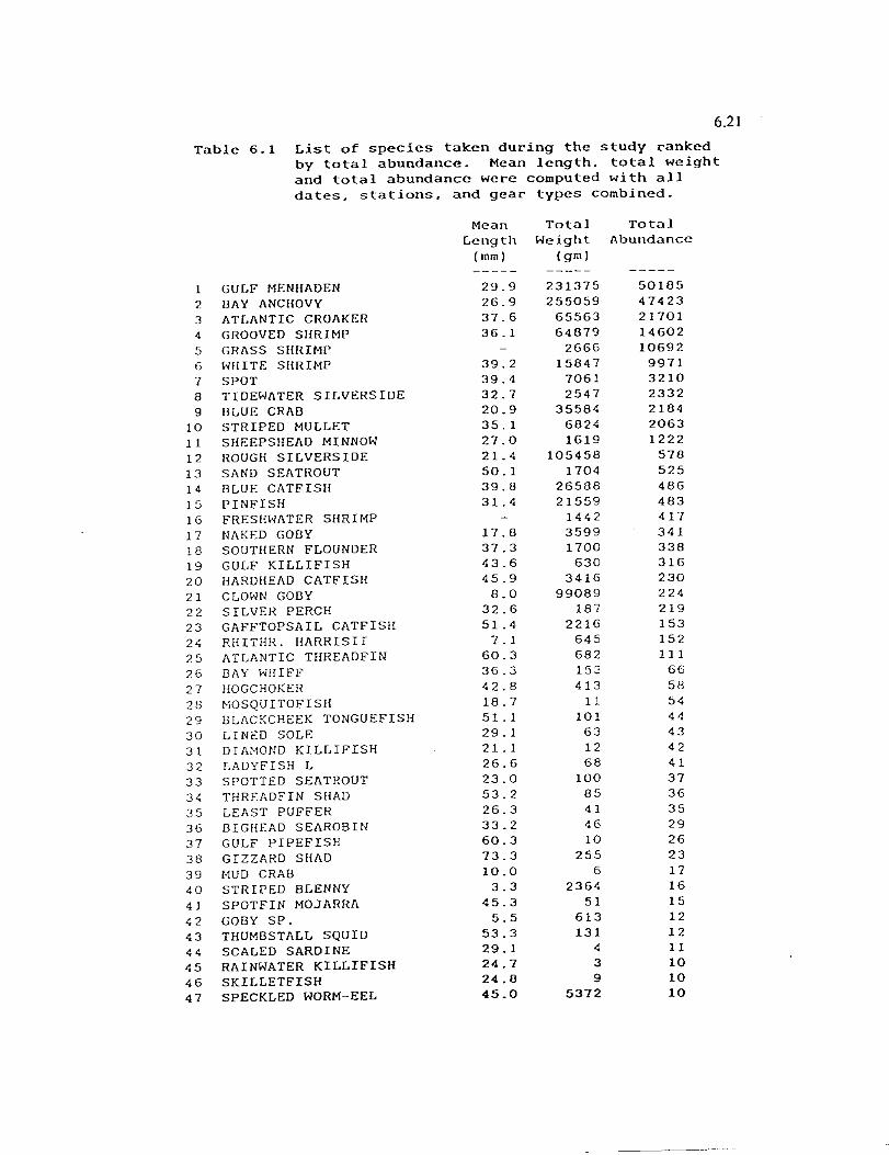
6.21

Table 6.1 List of species taken during the study ranked by total abundance. Mean length, total weight and total abundance were computed with all dates, stations, and gear types combined.

1 GULF MENHADEN 2 BAY ANCHOVY 3 ATLANTIC CROAKER 4 GROOVED SIIRIMP 5 GRASS SHRIMP 6 WHITE SHRIMP 7 SPOT 8 TIDEWATER SILVERSIDE 9 BLUE CRAB

10 STRIPED MULLET 11 SHEEPSHEAD MINNOW 12 ROUGH SILVERSIDE 13 SAND SEATROUT 14 BLUE CATFISH 15 PINFISH 16 FRESHWATER SIIRIMP 17 NAKED GOBY 18 SOUTHERN FLOUNDER 19 GULF KILLIFISH 20 HARDHEAD CATFISH 21 CLOWN GOBY 22 SILVER PERCH 23 GAFFTOPSAIL CATFISH 24 RHITHR. HARRISII 25 ATLANTIC THREADFIN 26 BAY l·mIFF 27 HOGCHOKER 28 MOSQUITOFISH 29 BLACKCHEEK TONGUEFISH 30 LINED SOLE 31 DIAMOND KILLIFISH 32 LADYFISH L 33 SPOTTED SEATROUT 34 THREADFIN SHAD 35 LEAST PUFFER 36 BIGIIEAD SEAROBIN 37 GULF PIPEFISH 38 GIZZARD SHAD 39 /·lOD CRAB 40 STRIPED BLENNY 41 SPOTFIN MOJARRA 42 GOBY SP. 43 THUMBSTALL SQUID 44 SCALED SARDINE 45 RAINWATER KILLIFISH 46 SKILLETFISH 47 SPECKLED WORM-EEL

Mean Length

(mm)

29.9 26.9 37.6 36.1

39.2 39.4 32.7 20.9 35.1 27.0 21.4 50.1 39.8 31.4

17.8 37.3 43.6 45.9 8.0

32.6 51.4

7.1 60.3 36.3 42.8 18.7 51.1 29.1 21. 1 26.6 23.0 53.2 26.3 33.2 60.3 73.3 10.0

3.3 45.3 5.5

53.3 29.1 24.7 24.8 45.0

Total Weight

(gm)

231375 255059

65563 64879

2666 15847

7061 2547

35584 6824 1619

105458 1704

26588 21559

1442 3599 1700

630 3416

99089 187

2216 645 682 153 413

11 101

63 12 68

100 85 41 46 10

255 6

2364 51

613 131

4 3 9

5372

Total Abundance

50105 47423 21701 14602 10692

9971 3210 2332 2184 2063 1222

578 525 486 483 417 341 338 316 230 224 219 153 152 111

66 58 54 44 43 42 41 37 36 35 29 26 23 17 16 15 12 12 11 10 10 10

6.22

Table 6.1 (continued)

48 DARTER GOBY 17.4 85 8 49 LADYFISH A 50.1 45 8 50 BLACK DRUM 28.4 286 7 51 ATLANTIC MIDSHIPMAN 39.3 25 6 52 RED DRUM 31. 7 129 6 53 SHEEPSHEAD 41.2 641 6 54 LEATHERJACKET 51.5 12 5 55 MENIPPE MERCENARIA 12.4 4 5 56 PETROLISTHES ARMATUS 6.6 1 5 57 INSHORE LIZARDFISH 33.8 40 4 58 XANTHIDAE SP. 5.0 0 4 59 ATLANTIC NEEDLEFISH 76.0 2 3 60 BAYOU KILLIFISH 36.3 3 3 61 CHAIN PIPEFISH 31.0 4 3 62 PIGFISH 15.0 0 3 63 SAILFIN MOLLY 28.0 1 3 64 GREEN GOBY 26.0 1 2 65 SOUTHERN KINGFISH 80.0 17 2 66 STRIPED ANCHOVY 40.0 1 2 67 ATLANTIC BUMPER 25.0 0 1 68 BLACK CRAPPIE 120.0 58 1 69 CENTRARCHID SP. 20.0 0 1 70 CLINGFISH 10.0 0 1 71 CODE GOBY 16.0 0 1 72 CRAVALLE JACK 96.0 25 1 73 EURYPANOPEUS DEPRESSUS 11.3 1 1 74 GULF KINGFISH 11. 0 26 1 75 GULF TOADFISH 11.0 46 1 76 LONGNOSE KILLIFISH 28.0 0 1 77 MOTTLED MOJARA 64.0 0 1 78 PAGURID SP 6.0 0 1 79 SHRIMP EEL 41.0 80 1 80 SOUTHERN HAKE 62.0 3 1 81 STAR DRUM 9.0 0 1 82 STRIPED BURRFISH 3.0 0 1 83 SUNFISH SP. 61.0 6 1 84 WHITE CRAPPIE 170.0 150 1

figure 6.1 Site/time dendrogram from cluster analysis of ichthyoplankton data.

85 JAN 1985 633 JAN 1985 633 NOV 1984 633 DEC 1985 603 JUN 1986 45 NOV 1984 603 DEC 1985 85 DEC 1985 613 AUG 1985 613 ocr 1985 65 NOV 1984 603 AUG 1985 603 NOV 1984

]------------------------------------------------------------------------------

--I --]------------1 1 1 ]---------1 1------------[ ----------[-[ [

------------[--[ [------------------------------[ ----------------------------) ) [

1-----------[

6~23

]

603 JAN 1985 603 APR 1985 613 MAR 1985 623 MAR 1985 65 APR 1985 603 MAR 1985 45 JAN 1985 65 MAR 1985 45 APR 1985 85 MAR 1985 65 JAN 1985 45 MAR 1985

------------1----------1 1------------------- ------------------[ ------------[ [--------------------[ ------------[----------[ 1

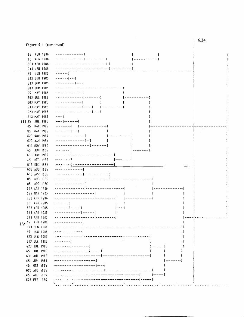
6.24 Figure 6_ I (continued)

65 FEB 1986 65 APR 1986 603 APR 1986 613 JAN 1985 85 JUN 1985 623 JUN 1985 633 JllN 1985 603 JUN 1985 65 MAY 1985 603 JUL 1985 603 MAY 1985 633 flAY 1985 623 MAY 1985 613 MAY 1985

III 45 JUL 1985 45 MAY 1985 85 flAY 1985 623 NOV 19St 623 JAN 1985 6ll NOV 19St 65 JUN 1985 613 JUN 1985 45 DEC 1985 613 DEC 1985 633 AUG 19S5 613 APR 1986 85 AUG 19S5 85 APR )986 623 APR 1986 633 flAR 19S5 633 APR 1985 85 APR 1985 633 APR 1985 613 APR 1985 623 APR 1985

IV t5 APR 1935 613 JUN 19S5 85 JUN 1986 623 JUli 1986 613 JUL 1985 623 JUL 1985 65 JUL 1985 633 JUL 1985 45 JUN 1985 45 OCT 1985 623 AUG )985 4S AUG 1985 623 FEB 1986

----------------) ----------------)------------1 -----------------------------1-)

1--------------1 I

-------------------------------)------------) -------)

-------)---)

-----------)----1 ----------------)----------------------1 ----------------) ----------------)---------1 1--------------) ---------------) ---------------)-----1 1------------1 ---------------------1----[ ----I

----1--------1 ---------1 1----------------1 1------------------------- ------------------, ---------)---1 ) -----------------[ 1-------------1 -----------------1--1 1 --------------------I---------j --------1 )---------1 --------1-------------------------1 1 ---------1 1---------1 ---------i------------------------l ----------------! ----------------)--------------{ -------------------------------1------------------------I -----------------j -----------------{----------------------) !-----------------! -----------------------1 -----------------------j-----------I {---------------j --------, { {

--------!------I {----{

---------------1-------1 -----------------------I-----------{ [----- ----------------------------------[ ----------------[--------------------------------------------------------[[ ----------------[ [[ ----------------)--------------------------------------I ----_----1

---------!----------[ 1-------1

{ 1 {I

!{

{ --------------------[------[ ---------------------------1---------------------------I ------------------------[ ------------------------{----[ -----------------------------{--------------------------I

!---------I [

-------------------------------------------------{ [------{

-------------------------------------------------[------[ ... _. _ ......••.••• "'or •••••••••••••• __ Of •••• -.--r"··· ...• , .• - •..•••.•••...••.•.••••.•...

Figure 6.2 Species dendrogram from cluster analysis of ichthyoplankton data.

BAY ANCHOVY CLOWN GOBY ROUGH S[LVERS[DE BLUE CRAB GULF MENHADEN BROWN SHR[MP NAKED GOBY ATLANT[C CROAKER STR[PED MULLET SPECKLED WORM-EEL P[NF[SH LEAST PUFFER T[DEWATER S[LVERS[DE WH[TE SHR[MP STR[PED BLENNY

------------------------[ ------------------------1----------[ -----------------------------------1---------[ ---------------------------------------------[--- ---[

----- ---- -------------------------[ ---------------------------------------[-----[ [------[

---------------------------------------------[--- -I ------------------------------------------------- 1-[ -------------------------------------------------1-1 I -----------------------------[ I -----------------------------1------------------- ---------I[ ------------------------------------------------- [[ -------------------------------------[ -------------------------------------[----[ 1--------[ ------------------------------------------[------ [

6.25

II

figure 6.3 Site/time dendrogram from cluster analysis of combined sled-seine data. 6.26

45 NOV 1984 623 NOV 1984 65 NOV 1984 613 NOV 1984 85 NOV 1984 603 JAN 1985 623 JAN 1985 613 JAN 1985 85 JAN 1985 65 JAN 1985 45 JAN 1985 45 DEC 1985 603 DEC 1985 65 DEC 1985 603 NOV 1984 613 DEC 1985 85 DEC 1985 623 DEC 1985 45 MAR 1985 65 MAR 1985 55 r~AY 1985 603 MAY 1935 613 JUN 1985 35 MAR 1985 633 AP.~ 1986 633 MAY 1985 45 MAY 1985 65 APR 1986 623 APR 1986 603 WR 1986 513 APR 1985 533 APR 1985 533 FEB 1985 503 APR 1985 623 APR 1985 65 APR 1985 85 M.AY 1985 523 MAY 1985 513 MAY 1985 613 MAR 1985 633 MAR 1985 623 MAR 1985 85 APR 1985 85 APR 1985 45 FEB 1986 45 APR 1986 65 FEB 1986 603 MAR 1985 45 APR 1985 613 FEB 1986 623 FEB 1986

------------------[ ------------------1--[ ---------------------1--------1 ---------------------1 [--------------[ ------------------------------1 -----------------[ -----------------[------1 ---------------------1 [ ---------------------1 [ 1--1 1- -----------------1 ----------------------[-[ [---------[

---------------------------1 ------------------[ ------------------1-------1 1-------1 --------------------------1------1 I ----------------------1 I ---------------------- I -- I I --- I

-------------------------1-1 ---------------------------1-----1 -----------------1 -----------------1----------1 ----------------------------1------1 -----------------------[ -----------------------1-------1 1-----1 ---------------1 I --------------- I -- I 1--- I

------------------1-------1 I --------------------------1----1 ------------------1

~~~~~~~~~ ~~~~~~~~~~~~~~~~---: ----------- I: -----1-- -----: ------------------------1---1 [I i 1

------------------------1 [[ ------------------------1-----------1 11 -------------------1 1 [I -------------------1----1 ------------------------1-------1 ----------------------1 1 [---I ----------------------I[ -----------------------1-------11 ------------------ [ I I --- I ------------------1------1 II -----------------1 [ 11 -----------------1 [ 1---1 11 ------------------[------[ I ------------------1 ------------------I[ I -------------------[----[ 1-1 ---------------------1 [--I [ ---------------------1--1 [[ ----------------[ ----------------[-1

[ [

H 1 1 1---------[

III

Figure 6.3 (continued) 6.27

603 FEB 1986 613 APR 1985 85 FEB 1986 633 DEC 1985 613 AUG 1986 613 AUG 1985 623 JUL 1985 623 AUG 1986 603 JUL 1985 613 JUL 1985 65 JUN 1986 65 JUL 1985 633 AUG 1985 633 AUG 1986 85 JUL 1985 85 JUN 1986 6 J 3 JUL 1985 65 OCT 1985 623 ocr 1985 623 AUG 1985 45 .AUG 1985 85 A.UG 1985 45 JUL 1985 55 AUG 1985 45 OCT 1985 85 OCT 1985 45 AUG 1986 503 OCT 1935 613 OCT 1985 533 OCT 1985 623 JUN 1985 5]3 JU!~ 1985 523 JUN 1986 65 AUG 1986 25 AUG !98~

603 JUN 1986 85 JUN 1985 633 JUN 1985 603 AUG 1985 45 JUN 1986 613 JUN 1985

603 AUG 1986 45 JUN 1985 65 JUN 1985 603 JUN 1985

------------------1------1 I ---------------------1 1-(

---------------------(---1 _________________________ ~_.---I--------l

--------------------------1-1 ----------------------------1---1 -----------------1 -----------------1----------( 1----( ------------------1 I ------------------1---1 1---1 ----------------------(1 I -----------------------1----( -------1

1----1 I

-------1------------------1 --------------------1 1-------1 --------------------1-----1 1--( ----------------------------------1 -------------1 -------------1-----------1 -------------------------1----1 -------------------1 -------------------11 --------------------1--------11-----1 ------------------- I II -------------------1---1 II

I 'I

i---- -------1

---------------------1 1-----1 ---------------------1-(

I 1----11

-----------------1 -----------------!-------------I

II II

-------------------------------! ----I I I -------------------------1 II -------------------------1-----1 II -------------------------------1-----1 I ----------------1 I I ----------------1-----1 ----------------------1-------1 ----------------------( 1--1 1---1 ----------------------1-------1 ------------------------ I I ------------------------(------1 1---1 ---------------------1 I ---------------------1---1 1-1 ---------------------- I I I I ----------------------1--1(----1 --------------------------1 ......................... - ..............•.......•........ , .... ........ .

Figure 6.4 Species dendrogram from cluster analysis of combined sled-seine data.

LEATHERJACKET MUD CRAB HARDHEAD CATFISH CLOWN G08Y SPOTFIN ~10JARRA

8LACKCHEEK TONGUEFISH SPOTTED SEATRDUT LADYFISH (adult) SCALED SARDINE LINED SOLE SKlLLETFISH BLACK DRUM DIAMOND KILLIFISH REO DRUM GULF PIPEFISH PINFISH

------------------------1 ------------------------1-------[ --------------------------------1-1 ----------------------------------1--1 ------------------------------1 I ------------------------------[--[ I-I ---------------------------------1-1 -----------------------------------1-1 I ---------------------------1 [ ---------------------------1-----------1 --------------------------1 [[ --------------------------[------------[ [[

-----------------------------------[ [[ -----------------------------------[---[ ------------------------------------[ ---------------------------------[ I

6.28

SOUTHERN FLOUNDER BAY WHIFF

---------------------------------[-[[-1 [-----------------------[

RHlTHR. HARRIS[ I DARTER GOBY BLUE C! TF I 5H FRESHWATER SHRIMP RAINWATER KILLIFISH MOSQU I TOF! SH LADYFISH (larvae) ATLANTIC CROAKER BLUE CRAB GRASS SHRIMP SPOT STRIPED MULLET 8ROWN SHR[MP T[DEWATER S[LVERS[OE GULF MENHADEN

-----------------------------------[1 I [ [ ------------------------------[ ------------------------------[---[ 1-----------------------------[ ----------------------------[-------[ -[

------------------------------------[-[ --------------------------------------[ --------------------------------------[--------------------------------[ -------------------------------[----[ -----------------------------------[[-[ -----------------------------------[[ [- ---j

--------------------------------------[ ------------------------------------[ ------------------------------------1 [ -------------------------------------[[

[------1 [ [

BAY ANCHOVY --------------------------------------[- --I SHEEPSHEAD M[NNOH ---------------------------------[ GULF K[LL[F[SH ---------------------------------[------ [--------------[

_~G~R::.:.AS::::S~SH:.:,[:.::MP~-------------------------------------------------------- -[- ---- [ S[LVER PERCH ---------------------------------------[ [ SAND SEATROUT WHITE SHRIMP NAKED GOBY ROUGH SILVERS[DE

::::::::::::::::::::::::::;--' ~ -: :' ----------------------------------[----- [[----[

---------------------------------------- I[ .. ... ... ... ... ••• "f ••••••• "r ••••••••••••••••••••••• • •• f···· ... of···· ....•...•

II

Figure 6.5 Site/time dendrogram from cluster analysis of trawl data.

45 ocr 1985 85 OCT 1985 65 AUG 1986 603 OCT 1985 613 OCT 1985 623 OCT 1985 45 AUG 1986 633 OCT 1985 45 JUL 1985 65 JUL 1985 623 JUL 1985 633 JUL 1985 613 JUL 1985 603 AUG 1986 503 JUL 1985 503 AUG 1985 45 AUG 1985 85 AUG 1986 613 AUG 1985 613 JUN 1986 623 AUG 1985 613 AUG 1986 85 AUG 1985 633 AUG 1985 623 AUG 1986 633 AUG 1986 35 .JUL 1985 65 AUG 1985 623 JUN 1986 633 JUri 1986 85 APR 1986 523 APR 1986 85 JUN 1986 633 APR 1986 613 APR 1986 623 MAY 1985 623 JUN 1985 613 MAY 1985 613 JUN 1985 603 APR 1986 603 MAY 1985 603 JUN 1985 85 JUN 1985 633 JUN 1985 603 DEC 1985 633 DEC 1985 85 DEC 1985 623 DEC 1985

--------------------1 --------------------1---1 ------------------------1------1 ----------------1 ----------------1-----------1 1-----------------1 ------------------------1 I I 1 ------------------------11 1--1 -------------------------1--1 -------------------1 -------------------1------------1 -------------------1 I --------------1 -------------------1----------1 1------1 -----------------1 I I I -----------------1----1 ]-] ------------------! 1-------1 ------------------1---1 -------------------------1 1---------] -------------------------1----------1 -------------------1 -------------------1----1 ----------------1 ----------------1-----1 1----1 -----------------) )-1 -----------------)----1

I--! I

------------------1 1------1 ------------------)-------1 -----------------------1 1--[ -----------------------1--1 -------------1 -------------1-------[ ----------------[ I-I ----------------1----1 1----[ -----------------------1 1---1 ----------------------------1 1------1 --------------------------------[ -------------1 -------------1--1 ----------------]-----------1 1---------- ---I ------------------1 ]----1 ------------------1---------1 ----------------------1 1-----1 ----------------------[------1 [ -----------------------1 1---1 -----------------------1-----1 ----------------------1 ----------------------]------1 ----------------------1 [ ----------------------1--1 1-----1

6.29

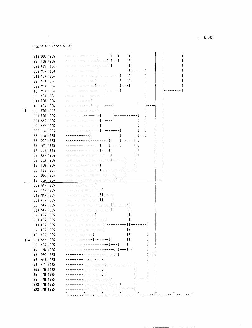
Figure 6.5 (continued)

613 DEC 1985 -----------------1 85 FEB 1986 -----------------1-----1 1---1 623 FEB 1986 -----------------------1-1 603 NOV 1984 ------------------1 1--------1 613 NOV 1984 ------------------1-----------1 I 85 NOV 1984 ----------------1 I 1 623 NOV 1984 ---------------- I -----1 1---- I 45 NOV 1984 ------------------1 1-------1 65 NOV 1984 ------------------1---1 613 FEB 1986 --------------1 I

45 APR 1986 --------------1-----------1 1-----III 603 FEB 1986 ----------------- I I

633 FEB 1986 -----------------1-1 1-------------1 633 MAR 1985 -------------------1------1 I 85 MAY 1985 -------------------1 603 JUN 1986 -------------------1----------1 65 JUN 1985 ------------- I I --- I

65 OCT 1985 -------------1----------1 1-------1 65 MAY 1985 ------------------- I 1-----1 45 JUN 1985 -------------------!----I 65 APR 1986 -------------------------1 I-I 65 JUN 1986 -------------------------1-------1 45 FEB 1986 ------------------- I I I

65 FEB 1986 -------------------1-----------1 1----1 65 DEC 1985 ----------------------------1 I-I

[

[----------1 I I

__ .:'..:...-~'C....'.= ___ --_--_-_--_-_--_-_--_-_--_-_--_-_--_--_-_--_--'-1-_--'-1 _____ ---11 --- I 45 JUN 1986

----------------1 IIII ----------------1---[ -------------------![-----I

603 ~IAR 1985 85 MAR 1985 613 MAR 1985 603 APR 1985 -------------------11 1 65 MAR 1985 -------------------------11--------1 623 MAR 1985 -------------------------11 623 APR 1985 ----------------1 633 APR 1985 ----------------1-----1 613 APR 1985 ---------------------11-----------11---------1 85 APR 1985 ---------------------11 II 45 APR 1985 --------------- I II

IV 633 ~IAY 1985 ---------------1--------1 II 65 APR 1985 ------------------------1----1 45 JAN 1985 ---------------------------1 [----[ 45 DEC 1985 ---------------------------1-1 1--- I

45 MAR 1985 ---------------------,1 45 MAY 1985 ----------------------[---------------1 603 JAN 1985 --------------------1 [ 85 JAN 1985 --------------------1-1 65 JAN 1985 ----------------------[--1 1------[ 613 JAN 1985 -------------------------[----[ [

623 JAN 1985 ------------------------------1-------[ •••••••• _ ••• of ••••••••••••••••• , ••••••••••••• ,- ··f···· ....•....

6.30

6.31

Figure 6.6 Species dendrogram from cluster analysis of trawl data.

BIGHEAD SEARDBIN NAKED GOBY RHITHR HARRISII MUD CRAB HOGCHOKER ATLANTIC MIDSHIPMAN LINED SOLE LEAST PUFFER PINFISH THUMBSTALL SQUID BLACKCHEEK TONGUEFISH BAY WHIFF ATLANTIC THREADFIN SHEEPSHEAD MINNOW GULF KILLIFISH THREAOF!N SHAD G IZZARD SHAD TIDEWATER SILVERSIDE SHEEPSHEAD STR] PED MULLET ATLANTIC CROAKER BROWN SHRli1P WHITE SHRIMP GAFFTOPSAIL CATFISH SILVER PERCH HARDHEAO CATFIS~ SAND Sf,TROUT BLUE CATFISH FRESHWATER SHRIMP BAY ANCHOVY BLUE CRAB GULF MENHADEN SOUTHERN FLOUNDER SPOT GRASS SHRIMP

-------------------------------1 -------------------------------11 --------------------------------1--1 -----------------------------------1--1 ----------------------------------1 ----------------------------------1---1-[ -----------------------------------1 I -----------------------------------1--1 -------------------------- ------ [ 1--- [ --------------------------------1-----[ --------------------------------1

--------------------------------[--[ 1-[ -----------------------------------1--[ [--------------1 ----------------------------------! ----------------------------------1------[ -------------------------------[ -------------------------------[---[ [-- [

----------------------------------11 ----------------------------------[[-----[ -----------------------------------1 --------------------------------[ --------------------------------1-"--1 -------------------------------------1-----------1 --------------------------------1 --------------------------------1--1 -----------------------------------1--1 --------------------------------------1-------1 I---------! -----------------------------------1 1 1 -----------------------------------1-------1 ---------------------------------i ---------------------------------1-1

1--1 I

-----------------------------------1--1 ! -- 1 --------------------------------------1-1 ----------------------------------------1 ----------------------------------------1--1

6.32

Table 6.2 Percentage of occurrence in each time/site group for each species in the icthtyoplankton data. Lines defining the boxes were derived from the dendrogram.

Time/site Groups

I II III IV

Bay Anchovy 1 89 10 Clown Goby 99 1 Rough Silverside 1 90 9 Blue Crab 5 50 5 Gult Menhaden 72 5 23 Brown Shrimp 1 16 83 Naked Goby 100 Atlantic Croaker 6 89 5 Striped Mullet 100 Speckled Worm-eel 100 Pinfish 100 Least Put fer 27 73 Tidewater Silverside 58 12 30 White Shrimp 69 31 Striped Blenny 35 65

Mean Salinity 8.7 4.0 3.6 10.9

Mean Temperature 22.8 16.6 23 .. 8 26.0

6.33.

Table 6.3 Percentage of occurrence in each ·time/si te group for each species in the combined sled-seine data.

Time/Site Groups

r--------I II III

Leatherjacket 100 Mud Crab 34 62 Hardhead Catf ish 100 Clown Goby 100 Spotfin Mojarra 18 82 Blackcheek Tonguefish 21 21 59 Spotted Seat rout 7 93 Ladyfish (adult) 100 Scaled Sardine 100 Lined Sole 100 Skilletfish 15 85 Black Drum 23 77 Diamond Killifish 98 Red Drum 50 50 Gulf Pipefish 43 36 21 Pinfish 4 94 3 Southern Flounder 96 4 Bay Whiff 90 11 Rhithr. harrisii 27 26 45 Darter Goby 22 78 Blue Catfish 30 70 Freshwater Shrimp 81 19 Rainwater Killifish 61 8 31 Mosquitofish 98 2 4 Ladyfish (larvae) 96 Atlantic Croaker 39 60 1 Blue Crab 31 43 26 Grass Shrimp 60 32 7 spot 7 89 3 Striped Mullet 93 6 1 brown Snrlmp 4 70 25 Tidewater Silverside 62 19 20 Gulf Menhaden 10 75 15 Bay Anchovy 18 1 59 Sheepshead l'-1innow 98 1 1 Gulf Killifish 97 2 1 Silver Perch 20 79 Sand Seatrout 90 10 White Shrimp 1 99 Naked Goby 28 20 51 Rough Silverside 6 94

Mean Salinity 4.4 6.8 9.1

Mean Temperature 10.8 22.3 28.3

-

6.34

Table 6.4 Percentage of occurrence In each time/site group for each species in the trawl data.

Time/site Groups

I II III IV

Bighead Searobin 6 89 5 Naked Goby 100 Rhithr. harrisii 9 13 43 35 Mud Crab 100 Hogchoker 40 20 2 39 Atlantic Midshipman 70 30 Lined Sole 66 27 7 Least Puffer 94 6 Pinfish 13 81 2 3 Thumbstall Squid 11 89 Blackcheek Tonguefish 38 28 34 Bay Whiff 24 68 8 Atlantic Treadfin 7 66 27 Saeepshead Minnow 1 8 92 Gulf Killifish 2 98 Threadfin Shad 17 2 81 Gizzard Shad 100 Tidewater Silverside 12 88 Sheepshead 16 84 Striped Mullet 7 15 78 Atlantic Croaker 2 67

I 6 -z4

Brown Shrimp 12 81 6 White Shrimp 43 56 Gaff topsail Catfish 100 Silver Perch 66 34 Hardhead Catfish 63 36 1

Sand Seat rout 36 52 7 6

Blue Catfish 63 9 1 26 Freshwater Shrimp 1 3 6 90 Bay Anchovy 34 35 II T<r Blue Crab 7 23 20 58 Gulf Menhaden 6 47 16 31

Southern Flounder 8 52 26 14

spot 3 83 6 14

Grass Shrimp 8 10 81

Mean Salinity 10.0 12.4 6.2 2.3

Mean Temperature 29.2 27.1 19.5 16.1

Table 6.5 ~onthly mean length (mm) by species, all stations combined. for the ichthyoplankton collections.

SPECIES November January Harch April May June July August October December February April June August Average s.d.

-----------------------------------------------------------------------------------------------------------------------------------------------------_. ATLANTIC CROAKER I 14.0 10.9 15.2 12.0 BAY ANCHOVY 1 20.0 21. 1 24.8 14.3 15.8 12 . 2 9. 7 17 . 0 20.3 5 . 3 20. 5

BLUE CATFISH BLUE CRAB 1 8.0 16.1 13.0 8.1 15.0 1.0 3.6 23.0

BROWN SHRIMP 1 13.0 12.4 1.8 13.8 10.4 11.9 CLOWN GOBY 1 5 . 5 4.S 4 . 0 4 . 0

FRESHWATER SHRIMP GAFFTOPSAIL CATFISH

GRASS SHRI~P GULF KILLIFISH

GULF ~ENHAOEN·I 20.7 23. 2 21.4 23.5 20.0 51.0 37 . 0 20.5 25. 2 HAROHEAO CATFISH

NAKED GOBY 1 3.5 PINFISH 1 12.0 14.0 13.0 12.0

ROUGHSILVERSIDEI 5.012.4 6.1 7.7 6.1 SAND SEAT ROUT 1

SHEEPSHEAD MINNOW 1 31.0 29.0 SILVER PERCH 1

SOUTHERN FLOUNDER I SPOT 1 8.0

SPOTTED SEATROUT I STRIPED ~ULLET 1

TIDEWATER SILVERSIDE 1 31.4 1.2 4.4 WHITE SHRIMP 1 9.0 8.5 9.0 11.0

Average s.d.

19.5 1 . 4

21.6 11.0

11.9 1.2

15.4 6.1

11. 1 5 . 7

14 . 6 15.1

13.8 12.0

8.0 2.6

10.3 9.5

16, 2 5. 9

16.8 5.3

13.3 8.0

20.5 0.0

____ e ........ ___ ..

13.3 2.3 16.5 5.1 0.0

11.1 6.3 11.6 2.2 4 . 5 0 . 1 0.0 0.0 0.0 0.0

26.9 10,4 0.0 3.5

12.8 1.0 1.5 2.9 0.0

30.0 1.4 0.0 0.0 8.0 0.0 0.0

16.3 18.3 U 1.1

14.6 9.2

0-w V1

Table 6.6 Monthly mean length (mm) by species. all stations combined. for the seine collections.

SPECIES Noyember January March April May June July August October Oecember February April June August Ayerage s.d.

--------------------------------------.-------------------.----.---------.------------------.. -------.-.----------------------------------------------- --------------AfLAHTlC CROAKER 17.8 17.1 25.5 37.6 44.3 64.3 74.8 63.0 13.5 21.4 19.0 41.7 80.3 100.0 44,3 21.8 BAY ANCHOVY 23.5 21.4 28.8 27.3 23.2 24 .8 27. 1 24.6 23.5 23.6 31. 1 28.3 25.1 28.9 25.8 2.8

BLUE CATFISH 139.6 11.5 40.0 33.0 12.5 12.0 13.0 57.0 40.0 43.6 BLUE CRAB 16.0 13.0 15.6 15.8 17 . 8 10.5 16.1 12.0 . 6.0 8.6 9.5 30.5 34.3 12.2 15.6 7.9

BROWN SHRIMP 29.4 13.6 17.6 28.8 52.5 41.1 25.9 50.5 16.0 15.3 40.4 47.1 41.6 32.3 14.1 CLOWN GOBY 0.0

FRESHWATER SHRIMP 0.0 GAFFTOPSAIL CATFISH 5U 54.5

GRASS SHRIMP 0.0 GULF KILLIFISH 45.0 34.3 39.0 56.3 49.0 56.0 26.0 33.1 60.0 44.3 11.9

GULF MENHADEN 21.1 22.3 22.4 22.2 22 . 2 31.0 38.5 33.3 21.1 21.6 22.5 32.8 43.1 21.4 1.6 HARDHEAD CATFISH 10.1 13.5 84.0 95.0 13.0 43 .2 42.4

NAKED GOBY 18.5 23.0 25.3 33.0 11 . 5 12.5 1.1 16.0 18.0 15.0 31.0 20.0 8.1 PINFISH I 12.0 20.0 14.3 11.0 38.0 56.0 80.0 11.0 14.5 21.4 65.5 74.5 35.9 26.1

ROUGH SILVERSIDE I 61.4 52.8 34.8 39.9 35.0 28.1 33.3 40.8 11.9 SAND SEATROUT I 36.6 41.5 34.8 49.8 45.8 41.1 6.2

SHEEPSHEAD MINNOW I 25.1 26.6 30.0 29.1 22.1 24.0 26.4 3.0 SILVER PERCH I 10.5 21 . 6 41.5 60.0 18.3 55.5 36.6 20.6

SOUTHERN FLOUNDER I 36.6 42.5 19.0 42.6 35.2 11. 1 SPOT I 12.3 16.1 28.4 46.5 59.9 13.0 81.0 11.0 11.0 38.0 50.0 55.8 40.8 24.1

SPOTTED SEATROUT I 18.5 35.1 16.4 31.0 13.8 20.0 23.1 10.4 STRIPED MULLET I 21.0 23.1 25.6 39.7 34 .9 66. 1 11.2 46.8 96.0 20.5 24.4 29.0 55.6 42.1 23.4

TIDEWATER SILVERSIDE I 28.5 31.9 35.4 50.1 28.6 23.1 35.8 36.2 31.1 25.1 n.6 34.3 33.1 1.1 WHITE SHRIMP I 43 .0 29.1 21.4 54.1 51.8 10.0 28.4 '2.2 35.8 14.1

AYerage 2et 22.6 25.1 42.4 33.4 38.7 42.1 31.1 39.2 23.3 22.9 30.4 45. 1 (2.3 33.1 s.d. 10.3 6.8 8.0 31.1 14 . 2 19.6 22.1 17.5 29.9 11.4 12.4 11. 1 23.8 23.0 20.2

a.. w a..

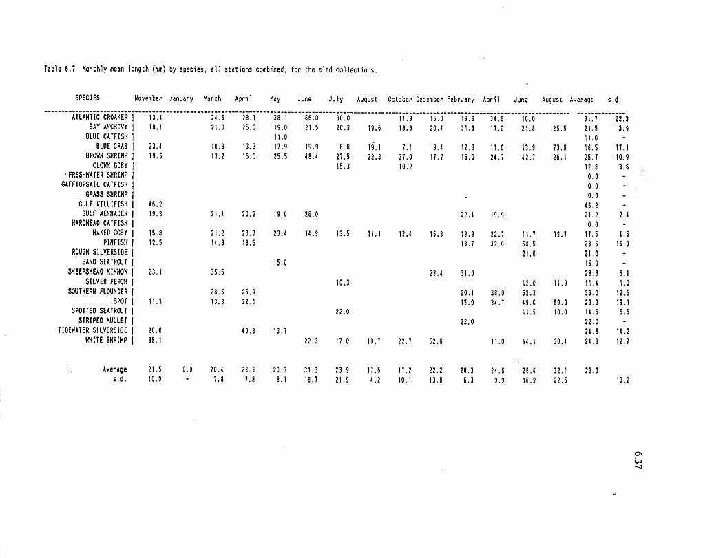
Table 6.7 Monthly mean length (mm) by species. all stations combined. for the sled collections.

SPECIES November January March April May June July August October Oecember February April June August Average s.d.

-------------------------------------------------------------------------------------------------------------------------------------------------------ATLANTIC CROAKER I 13.4 24.6 28.1 38.1 66.0 80.0 11.9 16.0 19.9 34.6 16.0

BAY ANCHOVY I 18.1 21.3 25.0 19.0 21.5 20.3 19.6 18.3 20.4 31.3 11.0 21.8 25.5 BLUE CATFISH I 11.0

BLUE CRAB I 23.4 10.8 13.3 11.9 19.9 8.8 19.1 1.1 9.4 12.8 11.6 13.9 13.0 BROWN SHRIMP I 19.6 13.2 15.0 25.5 48.4 27.5 22.3 31.0 11.1 15.0 24.1 42.7 26.1

CLOWN GOBY I 15.3 10.2 . FRESHWATER SHRIMP I

GAFFTOPSAIL CATFISH I GRASS SHRIMP I

GULF KILLIFISH I 46.2 GULF MENHADEN I 19.8 21.4 20.2 19.0 26.0 22.1 19.9

HARDHEAD CATFISH I NAKED GOSY I 15.8 21.2 23.7 23.4 14.9 13.5 11.1 13.4 16.8 19.9 22.1 11.1 19.1

PINFISH I 12.5 14.3 18.5 13.1 32.0 50.5 ROUGH SILVERSIDE I 21.0

SAND SEATROUT I 15.0 SHEEPSHEAO MINNOW I 23.1 35.5 23.4 31.0

SILVER PERCH I 10.3 12.0 11.9 SOUTHERN FLOUNDER I 28.5 25.9 20.4 38.0 52.3

SPOT I 11.3 13.3 22.1 15.0 34.1 49.0 60.0 SPOTTED SEATROUT I 22.0 11.5 10.0

STRIPED MULLET I 22.0 TIDEWATER SILVERSIDE I 20.0 40.8 13.7

WHITE SHRIMP I 35.1 22.3 11.0 18.7 22.1 52.0 11.0 14.1 30.4

Average s.d.

21.5 10.0

0.0 20.4 1.8

23.3 7.8

20.3 8.1

31.3 18.1

23.9 21.9

17.6 4 • 2

11 . 2 10.1

22.2 13.8

20.3 6.3

24.6 9.9

26 .4 16.9

32.1 22.6

------_ ... - ...... _--31.1 22.3 21.5 3.9 11.0 18.5 17.1 25.7 10.9 12.8 3.6 0.0 0.0 0.0

46.2 21.2 2.4 0.0

11.5 U 23.6 15.0 21.0 15.0 28.3 6.1 11. 4 1.0 33.0 12.5 29.3 19.1 14.5 6.5 22.0 24.S 14.2 24.8 12.1

23.3 13.2

C\ w .....,

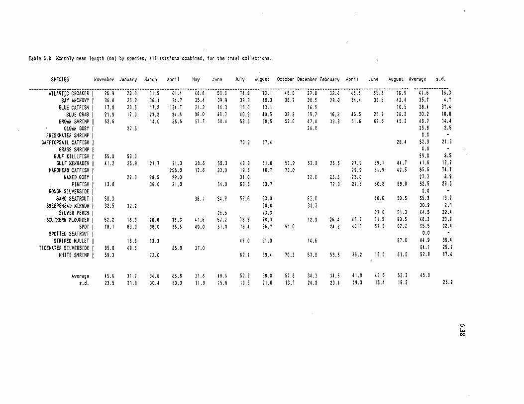
Table 6.8 Monthly mean length (mm) by species. all stations combined. for the trawl collections.

SPECIES November January March April May June July August October December Febru.ry April June August Average s.d.

--------ATLANTic-cROAKER-i----i6~9-----i3~o-----31~5-----il~i-----i8~8-----S8~6-----ii~8-----i3~1-----i6~o-----ii~8-----ji~i----is~s-----65~3-----io~9-

BAY ANCHOVY I 36.0 26.2 36.1 34.7 35.4 39.9 39.3 40.3 38.1 30.5 28.0 34.4 38.5 42.4 BLUE CATFISH I I1.D 20.5 11.2 134.1 21.3 IU 15.0 13:1 14.5 16.5

BLUE CRAB I 21.9 11.0 23.2 34.6 38.0 40.1 40.2 40.5 3U 19.1 16.3 H.5 25.1 26.2 BROWN SHRIMP I 51.6 1U 36.5 51.1 68.4 58.6 58.5 51.0 41.4 39.8 51.6 69.6 45.1

CLOWN GOBY I 21.5 14.0 FRESHWATER SHRIMP I

GAFFTOPSAIL CATFISH I 70.3 57.4 18.4 GRASS SHRIMP I

GULF KILLIFISH I 65.0 53.0 GULF MENHADEN I 41.2 25.9 27.1 31.3 38.6 58.3 48.8 61.0 57.9 53.0 26.6 17.9 39.1 44.7

HARDHEAD CATFISH I 156.0 13.6 33.0 19.6 40.7 73.0 79.9 31.9 42.5 NAKED GOBY I 21.0 28.5 19.0 31.0 32.0 25.5 13.0

PINFISH I 13.0 36.0 31.0 64.0 68.6 83.1 71.0 21.6 60.8 68.0 ROUGH SILVERSIDE I

SAND SEATRDUT I 58.3 38.1 54.8 51.6 63.0 81.0 40.0 53.6 SHEEPSHEAD MINNOW I 32.5 31.2 18.0 30.1

SILVER PERCH I 26.5 73.3 27.0 51.3 SOUTHERN FLOUNOER I 52.2 16.3 20.0 38.3 41.6 57.2 18.9 78.3 12.3 26.4 45.7 51.5 83.5

SPOT I 18.1 83.0 96.0 36.6 49.0 67.0 76.4 86.7 91.0 24.2 43.1 57.6 62.2 SPOTTED SEATROUT I

STRIPED MULLET I 16.6 13.3 41.0 91.0 14.6 87.0 TIDEWATER SILVERSIDE I 85.0 48.5 86.0 31.0

WHITE SHRIMP I 59.3 72.0 62.1 39.4 70.3 57.8 53.6 35.2 16.5 61.5

Average s.d.

45.6 23.5

31.1 21.8

34 . 6 30.4

65.8 83.3

31 . 6 11.9

48.6 15.6

52.1 19.5

58.0 21.0

57.6 13.7

34 . 3 24 . 0

34 . 5 20. 1

4 I .9 19.3

43.6 15.4

52.3 18.2

.... --............. _ .. __ .. 41.6 18.3 35.7 4.7 28.4 37.l 30.2 10.0 49.7 11.4 15.8 2.5 0.0

52.0 21.5 0.0

59.0 8.S 41.6 11.7 65.6 74.7 17.3 3.9 52.5 23.5 0.0

55.3 13.7 30.9 2.1 44.5 22.4 .s.3 23.9 65.5 22.4 . 0.0

41.9 36.4 64.1 25.1 52.8 17.4

45.9 26.9

0-w 00

T~ble 6.9 Monthly tot~l ~bundance for all stations by species in the ichthyoplankton collections

SPECIES November January March April May June July August October Oecember February April June August Average s.d.

_ ... _-----.-----------_.---------------------------------------------------------------------------------------------------------------------------------ATLANTIC CROAKER I 1 49 5 I BAY ANCHOVY I 61 59 37 H6 100 11 16 11

BLUE CATFISH I . BLUE CRAB I 38 I BROWN SHRIMP I 66 17 65

CLOWN GOBY I 17 183 FRESHWATER SHRIMP I

·GAFFTOPSAIL CATFISH I GRASS SHRIMP I

GULF KILLIFISH I GULF MENHADEN I 158 148 151 13 II

HAROHEAO CATFISH I NAKED GOay I 17

PINFISH I 1 ROUGH SILVERSIDE I 10 119 18 18

SAND SEATROUT I SHEEPSHEAD MINNOW I

SILVER PERCH I SOUTHERN FLOUNDER I

SPOT I SPOTTED SEATROUT I

STRIPED MULLET I 1 TIDEWATER SILVERSIDE I 11 19

WHITE SHRIMP I 11

Average s.d.

15.0 16.1

41.9 56.1

31. 3 58 .4

51.3 91. I

55. 3 64.6

60.5 81.8

7 .8 9. 5

3.0 1 . 5

3 . 0 1.8

8 . 5 10.6

1.\ 0.7

17 . 0 11.9

1.0 19.0

-----_ .. _------11.8 11.9 51.9 0.0 6.8

26.8 53.5 0.0 0.0 0.0 0.0

67.2 0.0

17.0 1.3

38.2 0.0 1.0 0.0 0.0 2.0 0.0 1.5

15.7 U

30.1

6U

12.7 30.1 87.1

9U

0.5 51.5

0.0

0.7 8.5 U

55 . 0

0-w \0

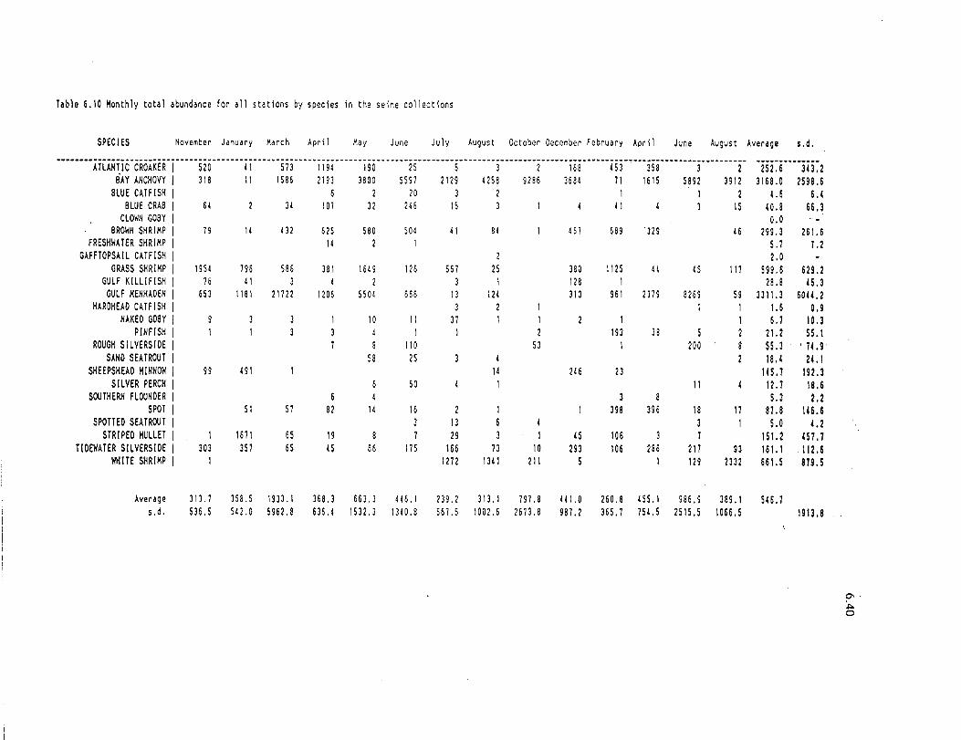
Table 6.10 Monthly total abundance for all stations by species in the seine collections

SPECIES November January xorch Apr i1 Hay June July August October December February April June August Average s.d.

.-~.-------------------------------------------------- ------------------------------------------------------ -----------------~------------------------- -------------. ATLANTIC CROAKER I 520 41 573 1194 190 15 5 3 1 168 453 358 3 2 252.6 343.2 S'AY ANCHOVY I 318 11 1586 1193 3800 5597 1119 4158 9286 3684 71 1615 5891 3911 3168.0 1598.6

SLUE CATFISH I 6 1 20 3 1 U 6.(

SLUE CRAS I 64 )( 107 31 146 15 41 15 40.8 66.3 CLOWN GOSY I 0.0

BR~N SHRIMP I 19 14 431 515 580 504 41 84 451 689 . 319 46 199.3 161.6 FRESHWATER SHRIMP I 14 1 5.1 1.1

GAFFTOPSAIL CATFISH I 2 1.0 GRASS SHRIMP I 1954 796 586 381 1649 116 567 15 380 1115 44 45 111 599.6 619.2

GULF KILLIFISH I 76 41 3 4 1 3 118 I 28.8 45.3 GULF MENHAOEN I 653 1181 11711 1206 5504 666 13 124 310 961 1379 8269 59 3311.3 6044.1

HAROHEAD CATFISH I 3 1 1 I I 1.6 0.9 NAKED GDSY I 10 II 31 I I I 6.7 10.3

PINFISH I 4 I 2 193 38 5 1 11.2 55,1 ROUGH SILVERSIDE I 8 110 53 I 200 8 55.3 '11.9

SAND SEATROUT I 58 15 2 18.4 21.1 SKEEPSHEAD MINNOW I 99 491 14 146 23 H5.1 192.3

SILVER PERCH I 50 11 12.1 18.6 SOUTHERN FLOUNDER I 6 3 8 5.3 2.1

SPOT I 51 51 81 14 16 1 398 396 18 17 87.8 H6.6 SPOTTED SEATROUT I 3 13 3 5.0 4.1

STRIPED MULLET I I 167 I 65 19 8 1 19 45 106 3 7 151.2 151.1 TIDEWATER SILVERSIDE I 303 357 65 45 66 115 166 13 10 293 106 286 217 93 161. I 112.6

WHITE SHRIMP I 1 1211 1341 211 5 119 1331 661.5 819.5

Average 313.1 358 . 5 1933 . I 368.3 663. 3 446. I 139. 1 313. I 191 . 8 441.0 160.8 455. I 986.9 389. I 546.7 s.d. 536.5 541.0 5961.8 636.4 1531. 3 1340.8 561 . 5 1001.6 1613.8 987.1 365.7 754,5 15 I 5.5 1066.5 1913.8

'" ~ o

Table 6.11 Monthly total abundance for all stations by species in the sled collections

SPECIES November January ~arch April May June July August October Oecember February April June August Average s.d.

--_.--------------.---.-----------------.-------------------------------------------------------------------------------------------------------------- --------------ATLANTIC CROAKER 116 90 51 6 1 1 15 64 46.6 61.1

,BAY ANCHOVY 14 11 41 13 12 86 18 4 16 13.5 11.4 BLUE CATFISH 1.0

BLUE CRAB 91 60 89 34 45 35 22 21 52 30 10 39.4 28.8 BROWN SHRIMP 11 131 175 165 101 181 61 18 811 1119 226 105 264.8 m.8

CLOWN GOBY 3.5 0.1 FRESHWATER SHRIMP 1.5 0.6

GAFFTOPSAIL CATFISH 0.0 GRASS SHRIMP 196 49 63 83 11 116 19 111 310 18 21 16 149.4 113.0

GULF KILLIFISH 11 11.0 GULF MENHADEN 4 1160 11 16 191.6 410.5

HARDHEAD CATFISH 0.0 NAKED GOBY 29 11 41 18 51 6 11 19 18.0 15.1

PINFISH 6 156 1 3 18.8 61.3 ROUGH SILVERSIOE I 1.0

SAND SEATROUT I 6.0 SHEEPSHEAO MINNOW I 169 15 49.3 80.6

SILVER PERCH I 21 91 40.3 44.3 SOUTHERH FLOUNOER I 18 13 3 9.4 10.3

SPOT I 33 361 1 58.4 133.9 SPOTTED SEATROUT I 3 1.3 1.2

STRIPED MULLET I 1.0 TIDEWATER SILVERSIOE I 1.0 1.2

WHITE SHRIMP I 01 86 21 161 80 100.0 15\.6

Average 53.4 286.0 169.0 43.3 35.5 38.6 93.2 34.3 16.3 31.5 148.6 116.2 49.9 25.6 15.3 s.d. 16.2 561.4 506.8 29.5 32.5 30.1 166.9 39.0 ERR 56.3 149.3 6.4 19.2 30.5 186.9

0-~

Table 6.12 Monthly total abundance for all st.tlons by specie in the trowl collections.

SPECIES November Janu,ry Horch April May June July August October December february April June August Average s.d.

........ ATLANTic.CROAKER.i· .. ··isj···.··iii··· .. iiij.····iisi·····issi·····iosi······iii······iii········S······iis······jii-···isis······iii······iii· ..... w ..... _. ___ • __

1159.9 1870.7 BAY ANCHOVY I 58 51 5J 62 81 9J 131 218 50 353 24 548 28 509

BLUE CATfISH I I 39 31 32 21 151 141 1 1 2 163.3 178.9 40.7 58.0

BLUE CRAB I 141 19 111 108 110 45 55 11 11 18 43 11 14 7U 81.9 BROWN SHRIMP I 113 36 190 1158 130 13 118 18 43 2111 1458 169 546.8 707.7

CLOWN GOBY 1.5 0.7 FRESHWATER SHRIMP I 111 168 5 98.5 12J.4

GAFFTOPSAIL CATFISH I 19 16 IS 50.3 23.8 GRASS SHRIMP I 411 481 41 49 IS 66 157.7 199.3

GULF KILLIfISH I 45 23.0 31.1 GULF MENHADEN I 141 110 116 318J JOl 117 83 17 101 157 1560 J58 316 497.9 862.2

HAROHEAD CATFISH I J 11 10 18 JJ 70 2l.5 28.0 NAKED GOBr I 1 1 1.6 0.5

PINFISH I 14 11 5. I 7.S ROUGH SILVERSIDE 0.0

SAND SEATROUT I 18 51 158 95 11 73 5J.( 53.7 SHEEPSHEAD MINNOW I 133 1 11 37.3 64.0

SILVER PERCH I 4 3 1 11 5.5 5.8 SOUTHERN FLOUNDER I 19 14 43 31 16 H 34 . ( 2 20.8 20.8

SPOT I 11 175 35 11 38 1300 ISO 40 136.5 35U SPOTTED SEATROUT I 0.0

STRIPEO MULLET I 64 18 15.7 21.5 TIDEWATER SILVERSIOE I 10 11.0 12.7

WHITE SHRIMP I 1047 656 209 134 131 15 563 316.2 532.5

Aver'ge s.d.

224.3 94.3 148.7 489.8 296.8 598.8 141.5 65.1 75.1

39.5 85.9 93.8 589.0 103.1 119.1 139.1 557.3 146.4 613.1 1051.9 479.9 1816.6 116.9 55.0 111.4 138.4 817.9 418.4 186.3 695.8

0-~ N

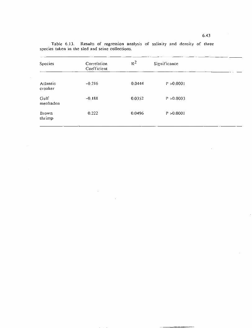
6.43

Table 6.13. Results of regression analysis of salinity and density of three species taken in the sled and seine collections.

Species

Atlantic croaker

Gulf menhaden

Brown shrimp

Correlation Coefficient

-0.216

-0.188

0.222

0.0444

0.0352

0.0496

Significance

P >0.000 I

P >0.0003

P >0.0001

~

N I [

CJ

o c

Q)

u c o

'" C ::J

D <{

3.00,-~~~~~~--~~~~~~~--~

::2.50

2.00·

1.50

1.00

+ c '0 0.50

E E ..c CJ' c OJ

v L

0 V c 0 ~

(fl

c 0 OJ :2

NDJFMAMJJASONDJFMAMJJA

Fig. 6.7 Mean n umber of Atlantic crooker· per 1 Om ~ 2 by

month for combined seine and sled dato

100

80

60

40

20

0

o-oTrowl t:. -6 Seine

NDJFMAMJJASONDJFMAMJJA

Fig 6.8 Mean length of Atlantic crooker from trawl

and seine data for each month

6.44

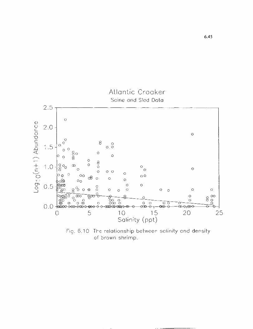
2.5

Q) () 2.0 c 0

D C :::; 1 .5 0 ~ « ..--...

+ 1 .0 c '-./

0

U> 0.5 0 ---.J

0.0 0

6.45

Atlantic Croakel' Seine and Sled Data

0

0

0 0 8 0

0.0 o 0 80 0

0 0 8 0 8 Q) 0

0 0 0 0 0

0 o 0 0

00 08 0 00

0 0 00 0 0

0 0 0 0 0 0 0

0 0 0 00 0 00

0 0 0 00 0 0

5 10 15 20 Salinity (ppt)

Fig. 6.10 The relationship between salinity and density of brown shrimp.

25

Brown Shrimp Seine and Sled Data

6.46

3.0.---------------------------------------~

~ 2.5-c o

-0 C ::J

..0 «

2.0 -o

o 0

8

o 00

°ao 00

8 0

o

o ~o

o ,

15 Salinity (ppt)

o o o

o

o 09 80 00 00

8 o

o

o o 0 0 00

o "

o o 0

6' o 0

o I~

20

o

8

o

Fia. 6.9 The relationshiD between salinitv and density

o

8 o o -

8

25

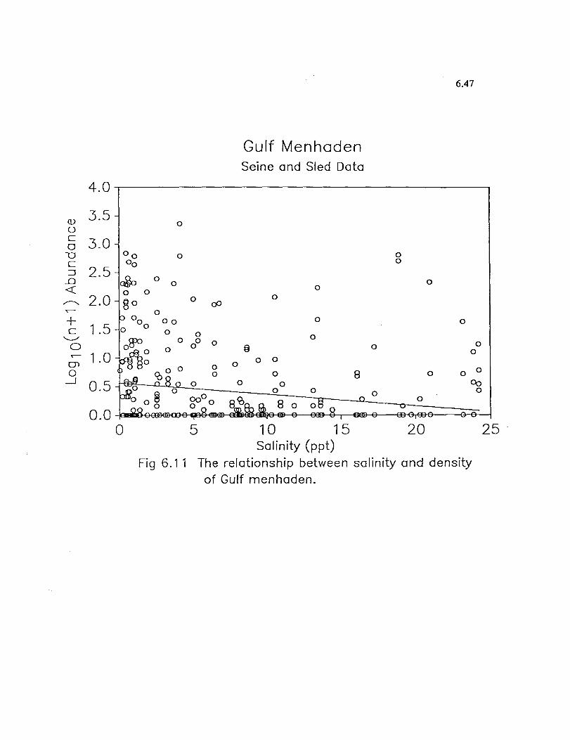
<l)

u c o u C :::::l

...0 «

+ C

'-..../

o

4.0

3.5

3.0

2.5

2.0

;;; 1.0 o

---1

0

0

o

0

0

00

o

o

0

0 00

o o 0 0 o

5

o o

o

Gulf Menhaden Seine and Sled Data

0

o 0

o

o

o

o

10 15 Salinity (ppt)

8

o

o o

20

o

o

6.47

o

o o

Fig 6.11 The relationship between salinity and density of Gulf menhaden.

25

7.1

CHAPTER 7

STABLE ISOTOPE STUDIES

INTRODUCTION

There are two stable isotopes of carbon and two of nitrogen with the

ratios:

1.11 0.37

12C 98.89 99.63

It has been known for sometime that these ratio values are slightly different

for materials from various sources. The chemical principles which control

these variations are well understood so that measurements of the ratios can be

used to study mechanisms of natural processes. As a result of small kinetic

isotope effects in the biological carbon and nitrogen cycles the major

reservoirs of carbon and nitrogen have fairly distinct isotope ratios. Modern

mass spectrometers make it possible to measure variations in these ratios on a

large number of samples at a high precision. By custom, isotope ratio data are

reported using the S (del) terminologyl.

Carbon reservoirs relevant to this study include C3 plants, phytoplankton,

seagrasses and C4 plants. Because these are the end members for the mixing

model that will be used to estimate the sources of organic matter in the diet

of animals it is important to note their S13C values as well as their abundance

x 1000

13 12 where Rx = CI C of a sample

13 12 Rs = CI C of a standard carbonate rock, PDB.

A similar definition applies to S1SN where the standard is atmospheric nitrogen. The units are per mil.

7.2

and distribution. Phytoplankton are distributed throughout the study area;

a13C for marine phytoplankton are - -20. The C3 plants are mostly associated

with the extensive Juncus marsh in upper Lavaca Bay and with other vascular

plant detritus which is being transported downstream by the river and streams;

aI3C for C3 plants is - -26. Seagrasses do not occur in Lavaca Bay, although

. B I3C f . they do grow In Matagorda ay; a or seagrasses IS - -10. Sparlina does

occur In upper Lavaca Bay, but it is not nearly as abundant as Juncus; as a C4

plant it has a aI3C of - -13. Given. these distributions and aI3

C ranges a

13 good, but not perfect, a C tracer model can be made for the study area.

To a first approximation a number of investigators have found that "you

are what you eat ± 1.0 per mil" applies to food webs as diverse as insects (Fry

et al 1978) and African browsing animals like the kudu (Van Der Merwe, 1982).

The opportunity for a natural tracer experiment of carbon flow in coastal food

webs is obvious and has been undertaken by several researchers. These studies

are reviewed by Fry and Sherr (1984).

Nitrogen isotope ratios, as expressed by .sI5N, do not behave exactly like

carbon. Rather than staying almost constant as organic nitrogen moves up a

food chain, aI5N shifts 2 to 5 per mil in the plus direction at each trophic

level (DeNiro and Epstein 1978). The exact value of this shift is species

dependent and is not well understood. However in a general sense the position

of a species in a food chain will be reflected in the a15N value of that

species. For example zooplankton are - +5, while raiilbow trout are - +12, in

Lake Iliamna, Alaska.

13 16 The results of a two year study of .s C and a N of the components of

the Lavaca River Delta and Bay are reported and analyzed in this report.

7.3

METHODS

Table 7.8 reports .s13C values for approximately 700 samples of biota,

sediment and dissolved organic carbon. In order to interpret this data an

estimate of error must be made.

The .s13C values were measured on a VG Micromass isotope ratio mass

spectrometer. The measurements were made on C02 which was prepared by

sealed tube oxidation, sample plus cupric oxide in a pyrex tube. Routine

duplicate analyses and daily calibration checks indicate that the analytical

error for a single analysis does not exceed ± 0.2 per mil. As may be

anticipated this is considerably less than the variability associated with

biological samples. Table 7.1 provides two examples of the range associated

with organisms taken in the same trawl haul.

These animals, like most in this study, are small and respond quickly to

changes In diet. The 1.0 to 1.5 per mil variability reflects the random

utilization of isotopically dissimilar diet items by these animals. Captive

shrimp offered a single diet resemble each other in .s13C values to ± 0.3

(Anderson et al 1987).

Samples were taken for isotopic studies during the regular sampling

periods, refrigerated, returned to the laboratory and kept frozen until

processed. The sampling schedule is shown in Table 7.2.

RESULTS

The major goal of the carbon isotope study was to assess the level of

utilization of river/marsh derived organic matter by biota in upper Lavaca Bay

and to establish whether a gradient of that organic signal extends toward the

lower bay. In order to evaluate the data-base (Table 7.8) it is necessary to

7.4

establish end members for the organic reservoirs which are subject to mixing.

The following values are consistent with generally accepted ones with the

major uncertainty being the net phytoplankton:

C3 terrestrial plants, e.g. elm C3 marsh plants, e.g. Juncus C4 marsh plants, e.g. Spartina Seagrasses Blue-green algae Net phytoplankton

- -26 - -26 - -13 - -10 - -14 - -20

The model for Lavaca Bay is a simple one wherein more negative organic

carbon derived from river transported C3 plants and from marsh derived Juncus

(also C3) is mixing with phytoplankton to yield organisms, sedimentary carbon

and DOC with intermediate 013C values. As has been pointed out seagrasses

are absent from Lavaca Bay and Spartina is not very abundant. For the

Matagorda Bay station seagrass must be taken into consideration.

A series of 013C measurements were made on gut contents and muscle

tissue to establish the relationship between the tissue and the most recent

feeding of each organism (Table 7.3). With only one exception, a flounder, the

animal tissue is between I and 3 per mil enriched in 13C (i.e. 013C more

positive) with respect to the gut contents. The muscle is a time integrated

quantity while the gut content is short term. Nevertheless it appears that

there is a small metabolic isotope effect for carbon. Other workers have made

similar observations for other ecosystems. Based on this argument one can

argue that 013C values of animal tissue shown in Table 7.8 should be corrected

I or 2 per mil to represent the food source. No such correction has been

made, but the argument should be kept in mind.

Marine sediments contain several types of organic matter including

macro-infauna which was removed. Thus 013C determined on the remaining

material provides data which should record a time integrated indicator of the

source of organic matter.

7.5

In Figure 7.1 al3e of all sediment samples are

plotted against station number to test the simple model that the amount of

river transported organic matter which is deposited in sediment decreases with

distance from the river. There is a clear trend which verifies the model;

station 623 does not fit the trend, being too heavy in al3e. The ordering of

the stations on the x-axis is somewhat arbitrary, but it does follow the

average salinity trend. The average al3e values for sedimentary organic

matter range between -22.5 and - I 7.5. This is not unexpected since even the

river station has a plankton source for some fraction of its organic matter.

The bay stations 1505, 1905 and 35/36 appear to have received very little river

transported higher plant organic matter. Once again station 623 is more

positive, 13e enriched, than the trend would place it.

Infauna were picked from sediment, identified and subjected to al3e

determination. The same trend IS seen for infauna (Figure 7.2) as for

sediment; a strong higher plant/river signal near the river which grades into a

phytoplankton signal at the bay station. Infauna are ideal organisms for 13e

tracer studies because they do not move substantial distances and thus make a

true record of ol3e of organic matter which comes their way. If -23 is taken

as the al3e value which represents a 50 percent higher plant source and a 50

percent plankton source then infauna from stations 45, 603 and 65 are mostly

higher plant supported while the other stations are mostly plankton based.

Station 623 is again a special case. Bivalves, like infauna, are non-mobile and

good ol3e recorders. Figure 7.3 shows a clear trend of al3e with distance

from the river mouth for bivalves. Bivalves are often used as indicators of

pollution and they may be useful indicators of the source of organic carbon.

7.6

Zooplankton are at the base of the food web and thus important to an

understanding of the food web. The samples shown in Figure 7.4 represent

hand picked zooplankton which are free of detritus. Each point represents

more than one species, but the species are known and recorded in Table 7.8.

Once again station 623 does not follow the trend. A strong input of river

transported higher plant material is suggested by the fact that the Lavaca

Bay/River stations (except 623) are more negative than -23.5. This observation

confirms the suggestion that Spartina is not very important in this food-web

relative to C3 material. 13 In order to more critically examine {j C zooplankton,

individual Acartia (100-200) were hand picked from selected collections and

submitted for 013C analysis. The Acartia show the same trend with relation to

station number (Fig. 7.5), as the mixed zooplankton but they have end members

of -21.8 and -26.4 similar to our model. Acartia fall on the river source side

of the mixing curve with an overall average of -24.0 ± 1.9. This supports the

idea that zooplankton may be deriving substantial nutrition from higher plant

detritus or from microorganisms that are consuming detritus. In other words

in this estuarine system zooplankton are not just consuming phytoplankton,

they are interacting with higher plant detritus. Crude net tows were also

studied, but that data is not included in Figures 7.4 or 7.5. It is included in

Table 7.8.

Particulate organic carbon, POC, contains zooplankton, phytoplankton and

The 013C values for POC in Fig. 7.6 do not correlate with station detritus.

location very well, but it is interesting to note that most values are more

negative than minus 23, indicating a strong river/C3 plant source; station 623

again bucks the trend. Based on the fact that strong C3 and weak C4 signals

have been detected in Figures 7.1 to 7.5 it seems clear that the Bay POC

7.7

values of -20.3 represents marine plankton and not a mixture of C3 and

C4!seagrass; open bay stations less negative than -20 may represent a seagrass

influence. Dissolved organic carbon, DOC, shows little relation to station and

only a modest river signal (Fig. 7.7). DOC is too complex to yield to a simple

model.

The fish samples were taken with the net used in the distribution and

abundance study, which catches fish of a few cm length. The plot of 013C of

all fish vs station number (Fig .. 7.8) shows a fairly strong correlation;

especially if station 623 is ignored. The average 013C values of all fish,

sorted by station range between -21.5 and -19.0, a range which in Figure 7.8,

is suggestive of plankton as a source of carbon. Since fish are one or more

steps up the trophic scale the small metabolic effect described in Table 7.3 is

probably shifting them 1.0 or 1.5 per mil in the plus direction relative to their

food. At this time it is not appropriate to make a correction based on this

but one should be aware of the idea. Not all individual fish fall in this

narrow range. Table 7.4 shows the average 013C value of the same 198 fish

sorted according to type wherein the range is -17.1 to -24.6. The average

013C value of all fish used in the study is -20.6 ± 2.6. Individual species do

not correlate with station as well as all species do, as shown in Figure 7.9.

13 Specialized feeding patterns for Cyprinodon (avg. 0 C = -17.3), and Fundulus

(avg. 013C = -17.6) are evident.

Shrimp are like fish in being mobile and thus more able to seek food.

13 The plot of 0 C of all penaeid shrimp (Fig. 7.10) shows a fairly strong

correlation with station. 13

The average 0 C values of all Lavaca Bay samples

are more positive than -23 suggesting a mixed higher plant and plankton food

source. The shrimp value at the Bay station (-17.4) compares with offshore

7.8

Gulf shrimp (-16.5) (Fry, 1981). However it is possible that both samples may

have been slightly influenced by seagrass. Shrimp taken from seagrass beds in

the Laguna Madre have 5I3

C values in the -12 to -13 range (Fry and Sherr,

1984). Table 7.5 shows 5I3

C of shrimp as a function of station and month.

July collections at the river stations stand-out, but the data is inadequate to

make a firm conclusion. The same trend is seen for 5I3

C of fish vs station

and time of collection (Table 7.6).

A suite of samples was selected for the determination of 5I5N. These

samples were subsamples of freeze-dried and powdered material for which 5I3C

had been determined. 5I5

N is not generally viewed as a tracer of the source

of organic matter, i.e. terrestrial plant vs phytoplankton. It is rather an

indicator of the level of an organism on the trophic food scale. The samples

were selected to span the trophic structure of the river/bay for 5I5

N

ecosystem. Table 7.7 illustrates this trophic relationship In a gross way.

Higher plants and macro algae are at the less positive end of the Table. The

trophic shift of 5I5

N, mentioned earlier, of 2 to 4 per mil is evident in Table

7.7 with infauna as a group being the most positive. This does not indicate

that infauna are at the top of the food-web, because no doubt several food­

webs are represented in the data. However it does indicate that infauna, fish

and shrimp are fairly near the top. Among fish, croaker at +13 to +14 are

higher than Cyprinodon at +7. In another study large redfish were + 17, clearly

a top carnivore. Station number was not expected to correlate with 5I5

N,

however based on Fig. 7.11 that expectation is reconsidered. Figure 7.11

shows a weak trend for 5I5

N to become more positive with distance from the

river. If higher plant organic nitrogen is +2 to +3, while phytoplankton

nitrogen is +5 to +7, then a weak station to 5I5

N relationship might be

7.9

superimposed over the stronger trophic nitrogen pattern.

relationships are interesting, at this time the data base is too small to

completely resolve specific food-webs. Almost all of the samples used for S13C

are achieved as a dry powder which could be used for future S15N studies.

CONCLUSIONS

The S13C data combined with a simple, conceptual mixing model indicate

that substantial river transported higher plant, C3 and marsh C4 plant organic

carbon is being taken up and assimilated by organisms in the Lavaca Bay

ecosystem. The degree of assimilation correlated with distance from the river

for sedimentary organic matter and for a number of biota. The utilization of

river transported organic matter is most intense in bivalves and surprisingly in

zooplankton, Acartia. Shrimp and infauna show the river signal but less so

than bivalves and Acartia. Fish show the least utilization of river transported,

C3-higher plants. This is taken to indicate a plankton rich diet because the

role of the sparse Spartina stands do not appear to be generally significant.

The generalizations, based on S13C data, combine with abundance data for the

various species indicate that river and its associated marsh is important in the

food-webs of the estuarine system. A similar, but much less extensive, one

13 year survey of S C of samples from the study area (Ward et al 1982) found

trends like those discussed. Taken together the two years of data of this

study and the one year survey are a sound argument for the importance of

freshwater for the Lavaca Bay system.

7.10

LITERATURE CITED

Anderson, R.K., A.L. Lawrence and P.L. Parker. (1987). 13 12

A Cj C tracer

study of the utilization of presented feed by a commercially important

shrimp, Penaeus vannamei, in a pond growout system. J. World

Aquaculture Society. 18(1).

DeNiro, M.J. and S. Epstein. (1978). Influence of diet on the distribution of

carbon isotopes in animals. Geochimica et Cosmochimica Acta. 42:495-

506.

Fry, Band E.B. Sherr. (1984). S13C measurements as indicators of carbon flow

in marine and freshwater ecosystems. Contribution in Marine Science.

27:13-47.

Fry, B., A. Joem and P.L. Parker. (1978). Grasshopper food web analysis: use

of carbon isotope ratios to examine feeding relationships among terrestrial

herbivores. Ecology. 59:498-506.

Van Der Merwe, N.J. (1982). Carbon isotopes, photosynthesis and archaeology.

American Scientist. 70:596-606.

Ward, G.H., Jr., N.E. Armstrong and J.M. Wiersema. (1982). Studies of the

effects of freshwater inflows into Matagorda Bay, Texas. Phase 3 final

report. Austin, TX: Espey, Huston & Associates and the University of

Texas at Austin; prepared for U.S. Fish and Wildlife Service, Division of

Ecological Services, Albuquerque, N.M. 1 vol.

Fl r,UR£ 7.1

L RVRCR B RY STUDY c. 13

C o PDB OF SED I HENf

7.11

-1 4. 0 +-_"'-----' __ ----L_--'--_-'---__ -'-------'_---'--_--"--_-+!

I -16.01

I

1 I

(0-18.0 i :c I ~ 1 ;.:0 -20. 01

i -22.0

~ ~ I (-

~ I r I

~ -24.0+---~~--~--~--.---.-~~-.---.---+1

603 623 633 BRY 45 65 613· 85

STR r I-ON

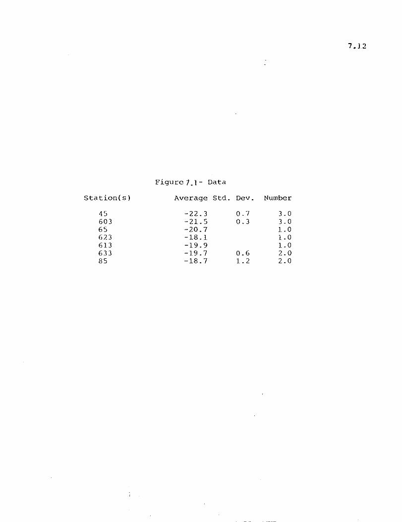
7.] 2

Figure 1.1 - Data

Station(s) Average Std. Dev. Number

45 -22.3 0.7 3.0 603 -21. 5 0.3 3.0 65 -20.7 1.0 623 -18.1 1.0 613 -19.9 1.0 633 -19.7 0.6 2.0 85 -18.7 1.2 2.0

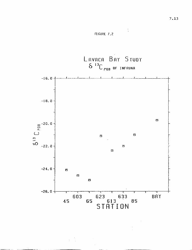
-16. 0 I

-18..1 ~

~ -20. 0 ~ "--

U en -yO

-22.0

-24.0

FI GURE 7.2

L RVRCR B RY S rUDY & 13 CPOB OF INFAUNR

I!l

7.13

I

[

-26. 0 +----r1 -----r----r-(!J --..,------,------,----,---'---.---+~ 603 623 633 BRY

45 65 613 - 85 STATIO-N

7~14

FIGURE 7.2 - DATA

Station(s) Average Std. Dev. Number

45 -24.1 2.54 13 603 -24.6 1.14 8

65 -25.0 1. 52 5 623 -21.1 0.87 6 613 -22.4 0.11 2 633 -22.0 1.80 9

85 -21.0 2.10 17

BAY -19.7 1. 45 68

ALL -21.1 2.49 128

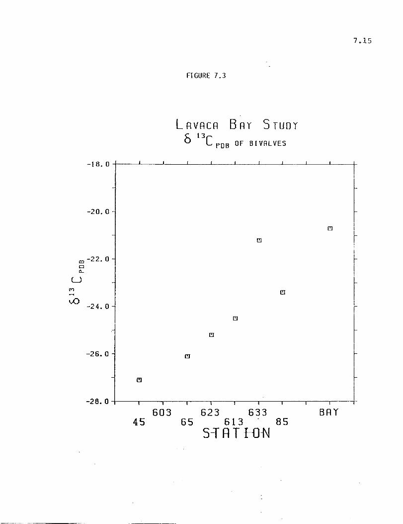
7.15

FI GURE 7.3

LAVACA BAY STUDY

& 13C POB OF BIVRLVES

-18.0+---~--L---L---L---L-~~~--~--~---+

-20.0

('] J I I r i

m -22.0 ~ Cl

i i a..

U I (Y1

~

\.0 -24.0 i I

~ .~

I -26.0 ('] I

~ I

I -28.0 I

603 623 633 BRY 45 65 613 85

S-T R T I{)-N

7.H

FIGURE 7.3 - DATA

Station(s) Average Std. Dev. (N)

45 -27.1 1 603

65 -26.1 1 623 -25.2 1. 55 4 613 -24.5 1. 34 3 633 -21. 2 2.31 4

85 -23.4 2.50 8

BAY -20.7 1. 44 5

ALL -23.2 2.69 26

7.<17

FI GURE 7.4

LRVRCR B WI' STUDY & 13 C rOB OF lOOPLANKTON

-21. 0 I I I

I -22.0 r

r Cl ~ lL

U ('")

~

\.0 -24.0

-25.0

-26.0+---~--~--~--~--~~~~--~--~---+

603 623 633 BRY 45 65 613· 85

STAT--lO-N

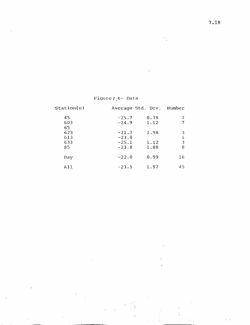
7.18

Figure 7.11 - Data

Station(sl Average Std. Dev. Number

45 -25.7 0.79 7 603 -24.9 1.12 7 65 623 -21.7 1. 98 3 613 -23.8 1 633 -25.1 1.12 3 85 -23.8 1. 88 8

Bay -22.0 0.99 16

All -23.5 1. 97 .1~ oJ

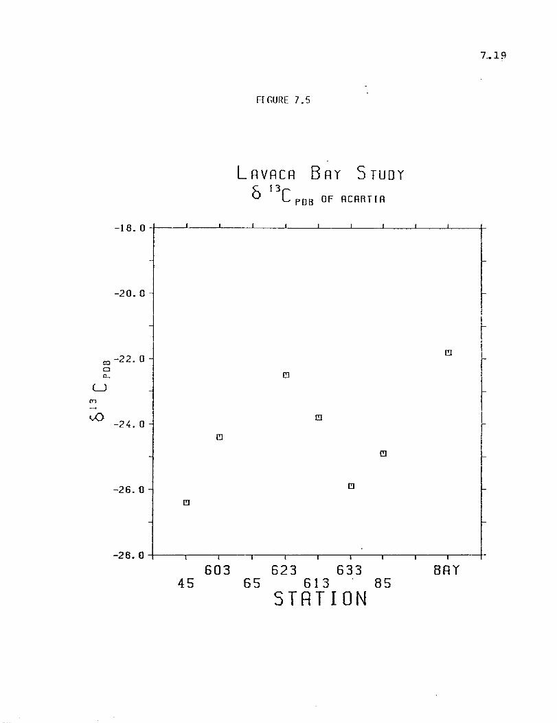
FI GURE 7.5

LAVACA BAY 5 TUDY & 13 C rOB Of ACARfIA

-18.0+---~--L---L---L-~--~---i __ -L __ -L __ ~

-20.0

l I

r I

c::l -22.0 Cl a...

U (T)

~

1.0 -24.0

-26.0

-28.0+---~--~--~--~~~~--~--~--~---+

603 623 633 BAY 45 65 613· 85

STATION

7;20

Figure 7.5- Data

Station(s) Average Std. Dev. Number

45 -26.4 0.30 3 603 -24.4 1. 26 4 65 623 -22.5 1 613 -23.8 1 633 -25.9 0.08 2 85 -24.9

Bay -21.8 0.92 6

All -24.0 1. 90 20

FIG@E 7.6

L RVRCR B RY 5 TUDY

& 13C rOB OF rac

7.21

-20.0T---~--~~--~--~--~--~--~--~--+

-21.0

l a:J -22. 0 ~ Cl ! n..

u

vO -23.0

-24.0

I!l -25.0+---~--~~~~--~--~--~--~--.---+

603 623 633 SRI 45 65 613· 85

STATION

7.22

FIGURE 7.6 - DATA

Station(s) Average Std. Dev. (N)

45 -23.2 1. 76 4 603 -24.9 1. 67 6

65 -23.7 2.82 3 623 -21. 8 0.42 3 613 -23 .. 8 1. 08 4 633 -23.9 0.23 2

85 -23.1 1. 40 5

BAY -20.3 1. 62 10

ALL -22.7 2.31 37

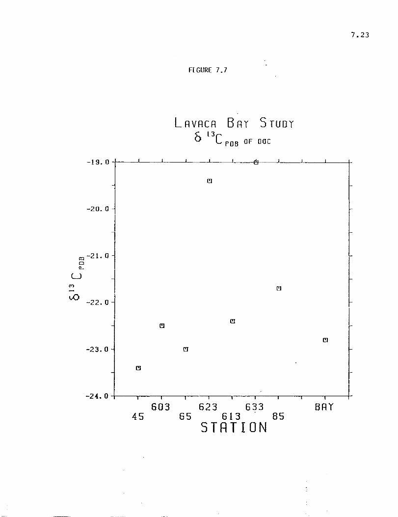
-19.0j

-20. 0 ~

CD -21. 0 Cl a...

u i 1..0 -22.0 i

-23.0

FI GURE 7.7

L RVRCR B RY 5 TUDY & 13C

rOB OF OOC

7.23

l

-24.0+---~--~~---.--~--~--~--~--~--+

603 623 633 BRY 45 65 613· 85

STRTION

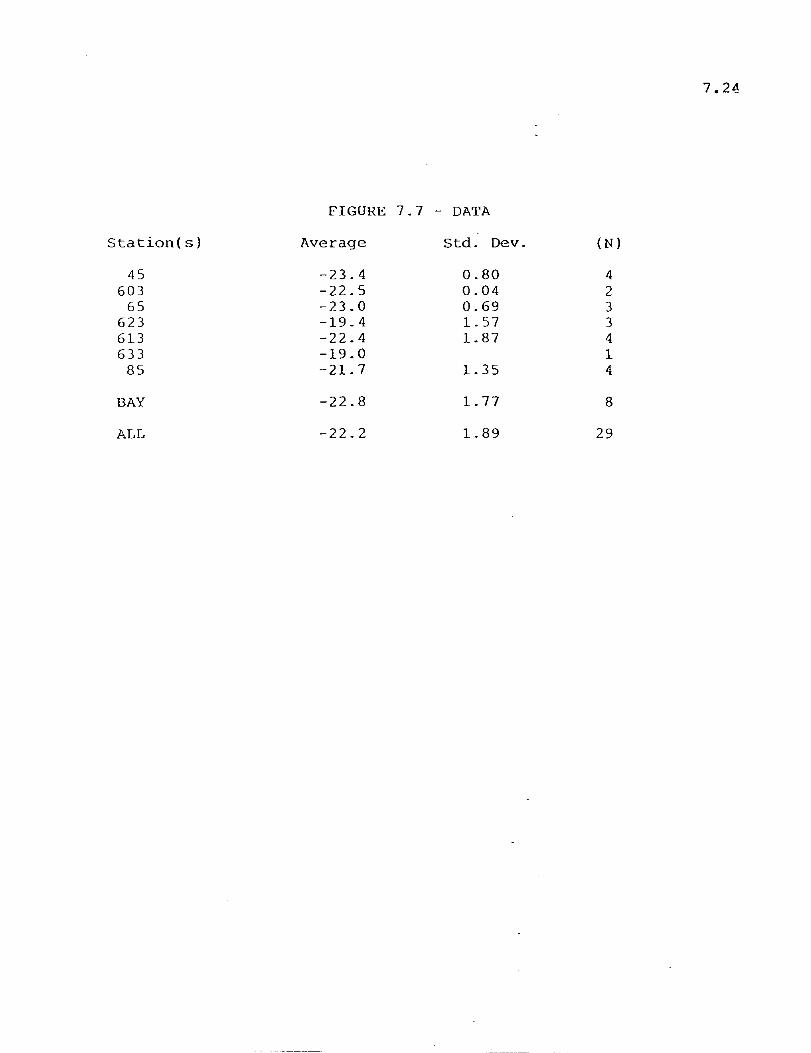
7.24

FIGURE 7.7 - DATA

Station(s) Average Std. Dev. (N)

45 -23.4 0.80 4 603 -22.5 0.04 2

65 -23.0 0.69 3 623 -19.4 1. 57 3 613 -22.4 1.87 4 633 -19.0 1

85 -21.7 1. 35 4

BAY -22.8 1. 77 8

ALL -22.2 1. 89 29

-19.5

lD -20. 0 o c....

u

vO -20.5

-21.0

7.25

FI GURE 7.8

LAVACA BAY STUDY

& 13C POB OF FiSH

-21.5+---~--~~--~--~--~--~--~--~--+

603 623 633 BAY 45 65 613· 85

STRTION

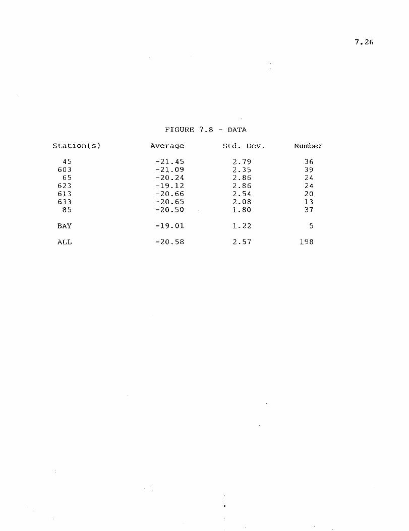
7.26

FIGURE 7.8 - DATA

Station(s) Average Std. Dev. Number

45 -21.45 2.79 36 603 -21.09 2.35 39

65 -20.24 2.86 24 623 -19.12 2.86 24 613 -20.66 2.54 20 633 -20.65 2.08 13

85 -20.50 1.80 37

BAY -19.01 1. 22 5

ALL -20.58 2.57 198

-18.0 I

-19. 0

m -20.0 0 0-

U (Yl -vO

-21. 0

-22.0

FIGURE 7.9

L RVRCR B RY 5 TUDY & 13 C rOB OF CROAKER + ANCHOVIES

7.27

I I I I

~

~ I

I ,

I

-23.0+---.----r---.---.--~--_.--_.--_.--_.,___r

603 623 633 BRY 4S 6S 613 8S

STATION

7.28

Figure 7.9- Data

Del 13-C Croaker

Station(s) Average Std. Dev Number

45 -22.3 1. 63 6 603 -22.4 1.60 7 65 -22.9 1. 42 7 623 -20.0 1. 97 5 613 -21. 5 1. 35 5 633 -19.9 2.04 4 85 -21. 9 1.16 12

Bay -21. 9 1.16 12

All -21.6 1.88 50

Del 13-C Anchovy

Station(s) Average Std. Dev Number

45 -22.0 1. 21 6 603 -21.7 1. 05 6 65 -22.7 0.28 3 623 -21. 4 0.23 2 613 -22.6 2.33 3 633 -21.8 0.88 3 85 -21.1 1.18 5

Bay -18.5 0.04 2

All -21. 6 1. 53 30

FI GURE 7.10

L RVRCR B RY 5 TUDY

& 13C POB OF PENAE[O SHRIMP

7.29

-14.0+---~--~--~--~--~--~--L---L---L---+

-16. 0

~ c:l-18. 0 ~ I

~ Cl I I a...

r u

(T1

~

....0 -20.0 r

I

-22.0

603 623 633 BRY 45 65 613· 85

STATION

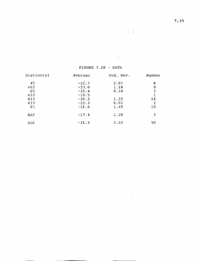
'7.30

FIGURE 7.10 - DATA

Station(s) Average Std. Dev. Number

45 -22.7 2.07 8 603 -23.0 1.18 9

65 -21. 4 0.34 3 623 -19.5 1 613 -20.2 1. 22 14 633 -22.3 0.02 2

85 -21. 6 1. 49 10

BAY -17.4 1. 28 3

ALL -21. 4 2.02 50

18. 0

16. 0

a: 14 . O l -a:

1 z til -1.0 12.0

,

i i

10. 0

8.0

(']

FI GURE 7.11

L AVACR B RY STUDY

& IS NAIR OF FISH

603 623 633 BAY 45 65 613 85

STATION

7. :n

~

7.32

FIGURE 7.11 - DATA

Station(s) Average Std. Dev. Number

45 9.10 2.82 3 603 12.80 0.67 3

65 0 623 0 613 0 633 0

85 12.23 2.25 6

BAY 14.58 0.00 1

ALL 11. 82 2.62 13

Individual I 2 3 4 5 6 7 8

x ± s.d.

* length in em

TABLE 7.1

S13C of Organisms Taken In the Same Trawl

Sta. 613 w. shrimp -21.39 (2)* -18.98 (2.5) -19.16 (3) -22.32 (3) -18.42 (3) -18.55 (3.5) -19.12 (3.5) -20.43 (6) -19.71 ± 1.52

Sta. 85 croaker

-22.46 (2.1) -23.24 (2.5) -23.18 (2.7) -23.13 (3.3) -22.28 (3.3) -22.52 (3.8) -22.27 (4.5) -20.10 (4.8) -22.4 ± 1.0 I

7.33

7.34

TABLE 7.2 SAMPLING SCHEDULE

ISOTOPE STUDY

Station Date 45 603 65 613 623 85 633 1505 1905 35/36

27-29 + + + + + + + Nov. 1984

22-24 + + + + + + Jan. 1985

2-3 + + + + + + + +s +s +s Apr. 1985

16-17 + + + + + + + Jul. 1985

22-24 + + +0 + + + + + Oct. 1985

4-5 + + + + + + + Feb. 1986

8-10 + + +POC + + + + + Apr. 1986

s = sediment only POC = water column POC only o = oysters only

7·.35

Table 7.3. Comparison of .sl3C values for muscle tissue and gut contents of some samples.

Size Species # (em) Muscle Gut Station Date

white shrimp 8 5 -24.3 "-27.2 45 7/85 Mullet 2 5 -19.2 -19.3 45 7/85 Menhaden 4 3.5 -24.6 -25.7 45 7/85 Blue catfish 2 9 -25.7 -27.0 45 7/85 Anchovy 12 2.5 -24.0 -26.4 45 7/85

Anchovy 6 2.5 -23.9 -25.7a 603 7/85 Sea trout 1 6 -21. 3 -22.0 603 9/85 Blue catfish 2 11 -24.7 -24.9 603 9/85 Croaker 4 7 -24.2 -26.4 603 7/85 Flounder 1 14 -21.3 -20.4 603 4/85 Flounder 4 7.5 -24.7 -26.0 603 7/85 Menhaden 2 4.5 -24.1 -24.5 603 7/85 Menidia 3 3.5 -23.5 -23.7 603 7/85 Mullet 2 7 -21. 6 -22.7 603 7/85 Brown shrimp 6 6 -23.3 -25.3 603 7/85 White shrimp 7 7.5 -23.2 -24.3 603 7/85

Croaker 3 5 -20.1 -23.2 65 4/85 Menhaden 8 2.5 -21.0 -26.2 65 4/85 Mullet 1 4 -17.5 -21. 2 65 4/85

Rangia 1 -24.0 -26.3 613 11/84 Menhaden 8 2.5 -20.8 -23.1 613 4/85 Anchovy 7 4 -20.7 -21. 5 613 4/85 Flounder 4 3 -20.4 -23.2 613 4/85 Croaker 8 3 -21. 0 -22.3 613 4/85

Macoma 1 -23.6 -23.9 633 8/85 Mullet 2 2.3 -19.6 -20.5 633 4/85 Anchovy 3 3 -22.6 -25.7 633 7/85

Paleomonetes 8 2.5 -18.2 -19.3 b 623 4/85

Anchovy 6 4.5 -22.9 -24.8 85 7/85 Anchovy 9 2.2 -21. 3 -21. 9 85 4/85 Croaker 6 3.5 -20.7 -22.0 85 4/85 Croaker 1 6 -19.6 -21.0 85 4/85 Fundulus 1 6 -17.7 -19.4 85 4/85 Hardhead catfish 1 12 -20.2 -22.2 85 7/85 Menhaden 7 2.5 -19.1 -20.6 85 4/85 Sea trout 1 4 -21.6 -23.2 85 7/85 Tonguefish 1 7.5 -20.9 -22.6 85 7/85

Species

Oyster Brown shrimp Macrobranchium Paleomonetes White shrimp

Oyster

a Whole animal.

b Eggs only.

c Fat only.

Size JL (cm)

2 5 4.5 1 3 6 3 5 7.5

2

7.36

2

Muscle Gut Station Date

-23.2 -25.5c 85 4/85 -22.2 -22.3 85 7/85 -19.1 -21. 6a 85 7/85 -19.3 -19.9 85 7/85 -22.5 -23.4 85 7/85

-20.3 -23.4a 1905 11/84

TABLE 7,4

De 1 \3-C Fish

i)e! 13-C of ~;electe(~ Fish Spec:ec.:,

{~nci·10VY

Calf;'3.h Croaj..:er

C'.,'P!" i I ;ooon r=-Ioundee

f7llllChl I uS

r-lenhaden 1 .... len 1 (; i cJ

i---j'l j j ~::' t

:';per k led Trout

--2 I t· -2<, _ i

-- 2 L ~)

- i? _-i

-~~ 1 n -17.6

-2 t.:=3 ·-20 .=-'

-is 8 -21 I

-22 (t

I_53 I _ 6 q

I _ BG

1 0..';

2 54 1 _ 7 0

i .92 1_65 j _ OS'

() 62

2.78

8 5(,

1 ~~

5

198

7.37

~; ~. ,] t ... ~ : ,

6'):1 !-,~~

h2~3

& j:3

CJ ~l:3 Fl:=;

,'I 1 1 ~ f\! i

os. ("1 ~

1 (\i'~

-20 _ 1

-It?i_H

- 20 ,--0

C.: C,( !

lteJ 13--l~ Sill-Imp

FFI3 -21 _~'

;~11) I I t. I I

{'lpr,

-22_() -20 _ :1 -22 _ f3

-1''1_'7 -- I l~ _ .:.

.J '" _ -2'-t _ ! -2."3_C?

-21.8 --2i.:3 -21.7 -(::1.3 --21.5 -21.9

-2 q --2 i - 3 --23 . 0 !, ( , ;::0 . .:) i 8 , " .

/, 56 2 5:"i I c'--? \! .

TABLE 7.5

m: 1 ND~'"

"C! ••. ' --2(; ()

-2(1 -, - C

-2(1 '. - 1 '7 ()

-~?(, - ~.!

_ ':.i:Jo '':;' L... ,_ • ,_ -2(1 _.

- I --:- _ ~. - I 7 . --

- ~

,I =' C' - -2() i .. - 2Li ; -!

! L~(~ I 35

7,. ::l8

A 1 j ( ;\1 ) -:;:. . (j . -"=>-:;:! 2 1 c '-' I 0'

~<-. . .J · · ,0

-22 1 I c 0 J oe ..J - · ' , -2 , .. :: 9 (i 2 O~ . - · .. '" 1 ''1 6 b · 0 i 3:.,

--2e- 2 i 5 - ':.) 1 - 1 8 -2 6 6 (; c~ · 1 '" - ~ 1 2 , 9 <) 1 -79

- 1 I, ~ (~ I L-;::'o -0> ·

-2 ! 2 qi) " i 2 .. L · qo - ; '", 2 j 2

. c (~ ~:

hc'.-_";' {. I '·1

;0. • ;j .

J(\li APn

. 1 U . '.':3 ·2<-~. r:~Z)

- 17 .. :'c·

-21 .79

- J 0 E12 {( ~?

2 ~~9

~i?1_1{1

- i:? 1 _ t".l.:l -;-~(i_8j

- 19. 5'? -2(1 _ ~;~.,

-2 ...... ',G -lC;_S:-~

.. ;~() . .:., 5 5~~

, 03 .

TABLE 7.6

1'1<' n 1. " J l·' '.- ne: 1 . 2', . 3::1 "-20 . ~j~

23 n-I .'1. .. - J 38

-2C~ 35 -2 J (,~ -;:<. i, !

-2 i J I - ! :~ 97

- 1 f1 Ci8

-c?2 93 -2r· . ! 5 2i.-, ~ ~

:=. :. 2 2"7

7.39

j·lll'i (1 i ! ; 1·1 ) s d -2n 2S - i~ I . ItS :36 ~

-:;C? .. c.:() ....... - ....

cP -;.? I (;9 3::;> c? 3:5 - i .. , .. .~o jJ'::' ;:!4 .J . ni, .. j <.' [~(J 1 '1 l 2 ::' ~ i? 8:~)

--(-~:) " , .. 2() D':.' 20 -,

~_~ L~

-2(; . c b .• 1 ! - 2 O~~

-2 1 . " ,. -20 5·) _ . , 8(;

-';~iJ '. ! - 1 '7 ~j l 5 22

-2(~1 3"'" -20 58 6:.3 2.2 2

t·_- ... -

Infauna Fish Oyster Shrimp Zooplankton (Acartia) Crab Bivalve (Rangia) Bivalve (Mulinia) Amphipods Detritus Sediment Plants

TABLE 7.7 6 1S N BY SAMPLE TYPE

6 lS N +11. 9"""±2. 6

11.6 + 2.5 11.4 + 1.1 11.1 ± 1.1 10.1 ± 0.5 10.0 ± 1.1 8.5 8.1 ± 0.2 7.6 5.9 ± 0.9 5.4 ± 5.4 4.7 ± 1.9

7.40

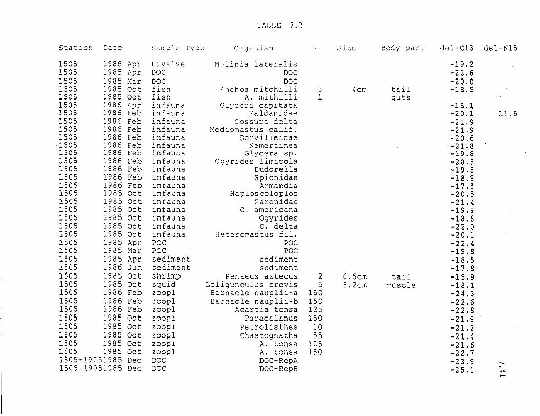
'['/\ULE 7.8

Station Date Sample 'l'ypcc Organism SLoe Body part del-C13 del-N15

1505 1986 Apr bivalve Mulinia lateralis -19.2 1505 1985 Apr DOC DOC -22.6 1505 1985 Mar DOC DOC -20.0 1505 1985 Oct fish Anchoa mi tchilli 3 4cm tail -18.5 1505 1985 Oct fish A. mithilli 1 guts 1505 1986 Apr infauna Glycera capitata -18.1 1505 1986 Feb infauna Maldanidae -20.~ 11.5 1505 1986 Feb infauna Cossura delta -21. 9 1505 1986 Feb infauna Mediomastus calif. -21. 9 1505 1986 Feb infauna Dorvilleidae -20.6

, ,1505 1986 Feb infauna Nemertinea -21. 8 1505 1986 Feb infauna Glycera sp. -19.8 1505 1986 Feb infauna Ogyrides 1imicola -20.5 1505 1986 Feb infauna Eudorella -19.5 1505 1'986 Feb infauna Spionidae -18.9 1505 1986 Feb infauna Armandia -17.5 1505 1985 Oct infauna Haploscoloplos -20.5 1505 1985 Oct infauna Paronidae -21. 4 1505 1985 Oct infauna G. americana -19.9 1505 1985 Oct infauna Ogyrides -18.8 1505 1985 Oct infauna C. delta -22.0 1505 1985 Oct infauna Heteromastus fil. -20.1 1505 1985 Apr POC POC -22.4 1505 1985 Mar POC POC -i9.8 1505 1985 Apr sediment sediment -18.5 1505 1986 Jun sediment sediment -17.8 1505 1985 Oct shrimp Penaeus aztecus 2 6.5cm tail -15.9 1505 1985 Oct squid Loligunculus brevis 5 5,2cm muscle -18.1 1505 1986 Feb zoopl Barnacle nauplii-a 150 -24.3 1505 1986 Feb zoopl Barnacle nauplii-b 150 -22.6 1505 1986 Feb zoopl Acartia tonsa 125 -22.8 1505 1985 Oct zoopl Paracalanus 150 -21. 9 1505 1985 Oct zoopl Petrolisthes 10 -21. 2 1505 1985 Oct zoopl Chaetognatha 55 -21. 4 1505 1985 Oct zoopl A. tonsa 125 -21. 6 1505 1985 Oct zoop1 A. tonsa 150 -22.7 1505+19051985 Dec DOC DOC-RepA -23.9 -...J

1505+19051985 Dec DOC DOC-RepB -25.1 . ..,. >--'

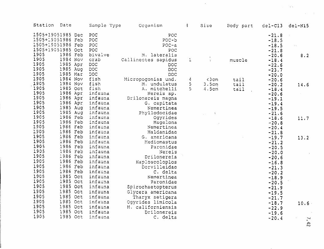
Station Date Sample Type Organism Size Body part del-Cl3 del-N15

1505+19051985 Dec poe POC -21. 8 1505+19051986 Feb poe Poe-b -18.5 1505+19051986 Feb poe poe-a -18.5 1505+19051985 Oct poe POC -21. 8 1905 1986 Feb bivalve r'1 . lateralis -20.6 8.2 1905 1984 Nov crab eallinectes sapidus 1 muscle -18.4 1905 1985 Apr DOC DOC -22.6 1905 1985 Aug DOC DOC -23.7 1905 1985 Mar DOC DOC -20.0 1905 1984 Nov fish Micropogonias undo 4 Ocm tail -20.6 1905 1984 Nov fish M. undulatus 5 3.5cm tail -20.2 14.6 1905 1985 Oct fish A. mi tchelli 5 4.5cm ta'il -18.4 1905 1986 Apr infauna Nereis sp. -20.6 1905 1986 Apr infauna Drilonereis magna -19.1 1905 1986 Apr infauna G. capitata -19.4 1905 1985 Aug infauna Nemertinea -19.5 1905 1985 Aug infauna Phyllodocidae -21. 6 1905 1986 Feb infauna Ogyrides -18.6 11.7 1905 1986 Feb infauna Magelona -20.8 1905 1986 Feb infauna Nemertinea -20.4 1905 1986 Feb infauna Maldanidae -21. 8 1905 1986 Feb infauna G. americana -19.7 13.2 1905 1986 Feb infauna Mediomastus -21. 2 1905 1986 Feb infauna Paronidae -20.5 1905 1986 Feb infauna Nereis -20.0 1905 1986 Feb infauna Drilonereis -20.6 1905 1986 Feb infauna Haploscoloplos -16.8 1905 1986 Feb infauna Dorvilleidae -21. 3 1905 1986 Feb infauna e. delta -20.2 1905 1985 Oct infauna Nemertinea -18.9 1905 1985 Oct infauna Paronidae -20.5 1905 1985 Oct infauna Spirochaetopterus -21. 9 1905 1985 Oct infauna Glycera americana -19.5 1905 1985 Oct infauna Tharyx setigera -21. 7 1905 1985 Oct infauna Ogyrides limicola -18.7 10.6 ' 1905 1985 Oct infauna 11. californiensis -22.9 1905 1985 Oct infauna Drilonereis -19.6 1905 1985 Oct infauna C. delta -20.4 .......

-l'> N

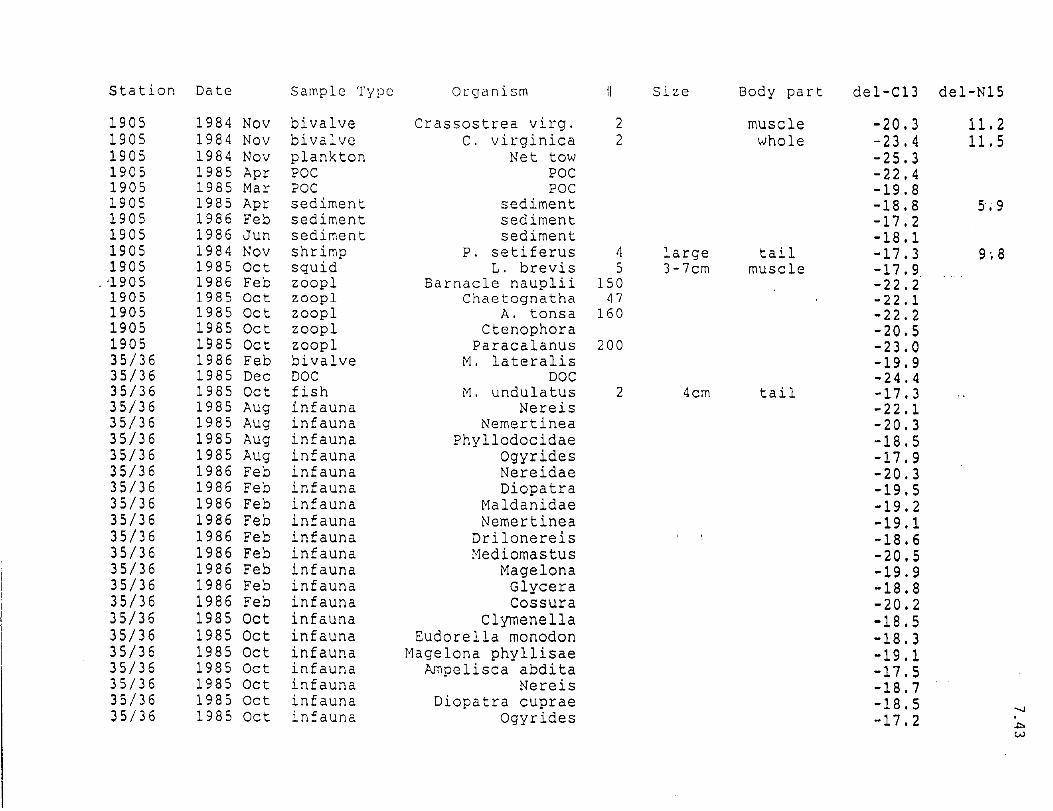
Station Date Sample Type Organism Size Body part del-e13 del-N15

1905 1984 Nov bivalve Crassostrea virgo 2 muscle -20.3 11.2 1905 1984 Nov bivalve C. virginica 2 whole -23.4 11.5 1905 1984 Nov plankton Net tow -25.3 1905 1985 Apr POC POC -22.4 1905 1985 Mar poe poe -19.8 1905 1985 Apr sediment sediment -18.8 5;9 1905 1986 Feb sediment sediment -17.2 1905 1986 Jun sediment sediment -18.1 1905 1984 Nov shrimp P. setiferus I) large tail -17.3 9;8 1905 1985 Oct squid L. brevis 5 3-7cm muscle -17.9

, '1905 1986 Feb zoopl Barnacle nauplii 150 -22.2 1905 1985 Oct zoopl ehaetognatha 47 -22.1 1905 1985 Oct zoopl A. tonsa 160 -22.2 1905 1985 Oct zoopl Ctenophora -20.5 1905 1985 Oct zoopl Paracalanus 200 -23.0 35/36 1986 Feb bivalve M. lateralis -19.9 35/3 6 1985 Dec DOC DOC -24.4 35/36 1985 Oct fish N. undulatus 2 4cm tail -17.3 35/36 1985 Aug infauna Nereis -22.1 35/36 1985 Aug infauna Nemertinea -20.3 35/36 1985 Aug infauna Phyllodocidae -18.5 35/3 6 1985 Aug infauna Ogyrides -17.9 35/36 1986 Feb infauna Nereidae -20.3

'35/36 1986 Feb infauna Diopatra -19.5 35/3 6 1986 Feb infauna Maldanidae -19.2 35/3 6 1986 Feb infauna Nemertinea -19.1 35/36 1986 Feb infauna Drilonereis -18.6 35/36 1986 Feb infauna Nediomastus -20.5 35/36 1986 Feb infauna Magelona -19.9 35/36 1986 Feb infauna Glycera -18.8 35/36 1986 Feb infauna Cos sura -20.2 35/36 1985 Oct infauna Clymenella -18.5 35/36 1985 Oct infauna Eudorella monodon -18.3 35/3 6 1985 Oct infauna Nagelona phyllisae -19.1 35/36 1985 Oct infauna Ampelisca abdita -17.5 35/3 6 1985 Oct infauna Nereis -18.7 35/36 1985 Oct infauna Diopatra cuprae -18.5 " 35/3 6 1985 Oct infauna Ogyrides -17.2 ..,.

w

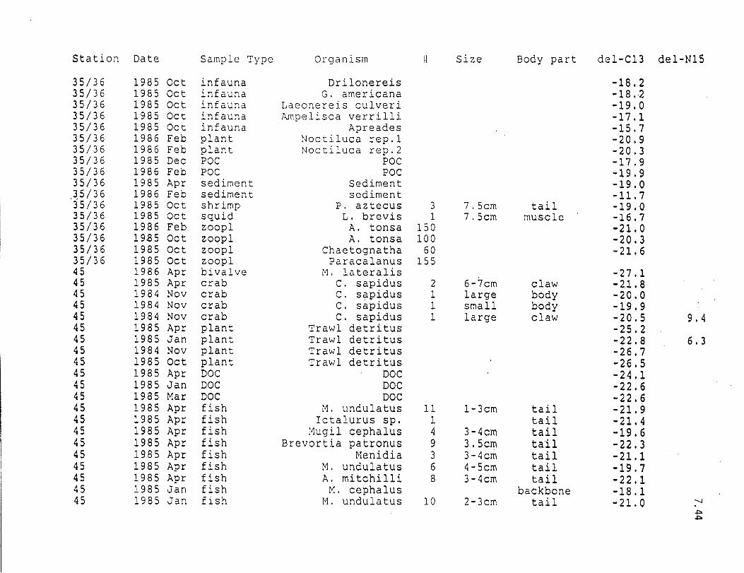
Station Date Sample Type Organism Size Body part del-Cl3 del-N15

35/36 1985 Oct infauna Drilonereis -18.2 35/3 6 1985 Oct infauna G. americana -18.2 35/3 6 1985 Oct infauna Laeonereis culveri -19.0 35/3 6 1985 Oct infauna Ampelisca verrilli -17.1 35/3 6 1985 Oct infauna Apreades -15.7 35/3 6 1986 Feb plant Noctiluca rep.l -20.9 35/3 6 1986 Feb plant Noctiluca rep.2 -20.3 35/3 6 1985 Dec poe poe -17.9 35/3 6 1986 Feb poe poe -19.9 35/3 6 1985 Apr sediment Sediment -19.0 )5/36 1986 Feb sediment sediment -11. 7 35/36 1985 Oct shrimp P. aztecus 3 7.5cm tail -19.0 35/3 6 1985 Oct squid L. brevis 1 7.5cm muscle -16.7 35/3 6 1986 Feb zoopl A. tonsa 150 -21. 0 35/3 6 1985 Oct zoopl A. tonsa 100 -20.3 35/3 6 1985 Oct zoopl Chaetognatha 60 -21. 6 35/36 1985 Oct zoopl Paracalanus 155 45 1986 Apr bivalve M. lateralis -27.1 45 1985 Apr crab C. sapidus 2 6-7cm claw - 2.1. 8 45 1984 Nov crab e. sapidus 1 large body -20.0 45 1984 Nov crab e. sapidus 1 small body -19.9 45 1984 Nov crab e. sapidus 1 large claw -20.5 9.4 45 1985 Apr plant Trawl detritus -25.2 45 1985 Jan plant Trawl detritus -22.8 6.3 45 1984 Nov plant Trawl detritus -26.7 45 1985 Oct plant Trawl detritus -26.5 45 1985 Apr DOC DOC -24.1 45 1985 Jan DOC DOC -22.6 45 1985 Mar DOC DOC -22.6 45 1985 Apr fish ~1. undulatus 11 1-3cm tail -21. 9 45 1985 Apr fish Ictalurus sp. 1 tail -21. 4 45 1985 Apr fish t'1ugil cephalus 4 3-4cm tail -19.6 45 1985 Apr fish Brevortia patronus 9 3.5cm tail -22.3 45 1985 Apr fish Menidia 3 3-4cm tail -21.1 45 1985 Apr fish M. undulatus 6 4-5cm tail -19.7 45 1985 Apr fish A. mitchilli 8 3-4cm tail -22.1 45 1985 Jan fish M. cephalus backbone -18.1 45 1985 Jan fish M. undulatus 10 2-3cm tail -21. 0 " . ..,. ..,.

Station Date Sample Type Organism Size Body part del-Cl3 del-N15

45 1985 Jan fish M. cephalus l3cm skin -16.3 45 1985 Jan fish A. felis 2 20cm tail -24.1 45 1985 Jan fish M. cephalus muscle -18.0 45 1985 Jan fish ~l. cephalus 10 2-3cm , whole -19.1 45 1985 Jan fish M. cephalus 13cm liver -20.4 45 1985 Jan fish M. cephalus 13cm scales -14.1 45 1985 Jan fish Cyprinodon varie. 10 2-3cm tail -17.6 45 1985 Jan fish B. patronus 10 2cm tail -21. 8 45 1985 Jan fish Menidia sp. 5 4.2cm tail -19.4 45 1985 Jan fish B. patronus 5 2cm whole -22.7 4.5 1985 Jan fish Fundulus simi lis 2 >3cm tail -22.2 '45 1985 Jul fish M. cephalus 2 guts -19.3 45 1985 Ju1 fish Ictalurus sp. 2 guts -27.0 45 1985 Jul fish M. cephalus 2 5cm tail -19.2 45 1985 Jul fish B. patronus 4 3.5cm tail -24.6 45 1985 Jul fish Menidia sp. 4 3-4cm tail -21. 7 45 1985 Jul fish Ictalurus sp. 1 3cm tail -26.8 45 1985 Jul fish B. patronus 4 guts -25.7 45 1985 Jul fish Ictalurus sp. 2 9-l0cm tail -25.7 45 1985 Jul fish M. undulatus 1 7cm tail -24.5 45 1985 Jul fish A. mi tchi 11i 12 guts -26.4 45 1985 Jul fish Trinectes maculatus 1 5cm tail -28.3 45 1985 Jul fish A. mitchi11i 12 2-3cm tail -24.1 45 1984 Nov fish B. patronis 1 4cm tail -23.3 45 1984 Nov fish M. undulatus 10 smiJ.ll tail -22.8 45 1984 Nov fish Menidia sp. 8 tail -20.4 45 1984 Nov fish A. mitchilli 10 large tail -22.4 45 1984 Nov fish F. similis 1 4cm tail -16.0 45 1984 Nov fish C. variegatus 1 2. Scm tail -17.5 7.3 45 1984 Nov fish A. mitchilli 20 small tail -22.3 45 1984 Nov fish F. similis 1 6cm tail -16.6 45 1984 Nov fish M. undulatus 10 large tail -23.8 13.1 45 1984 Nov fish C. variegatus 1 3.5cm tail -17.4 6.9 45 1985 Oct fish A. mi tchilli 8 1.8cm tail -20.4 45 1985 Oct fish A. mitchi11i 6 3.7cm tail -20.6 45 1985 Apr infauna Myrophis 1 -21. 7 45 1985 Apr infauna Chironomid larvae -29.0 45 1986 Apr infauna Laeonereis culveri -20.7 .......

.p. . U1

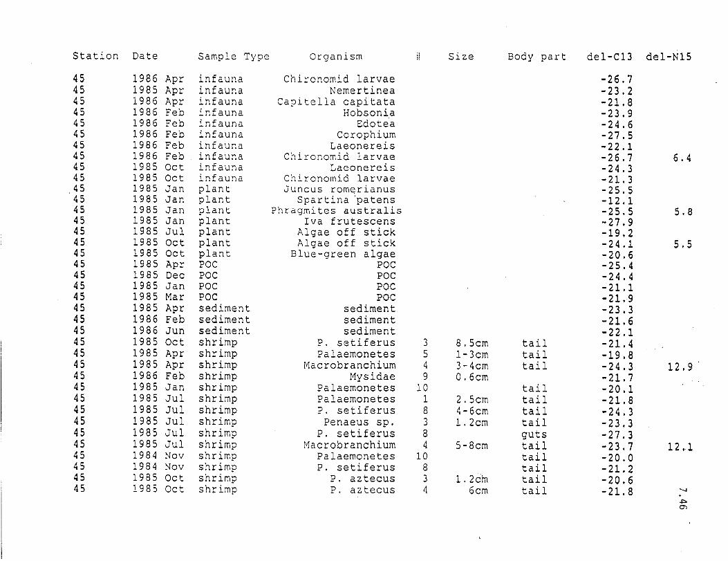
Station Date Sample Type Organism Size Body part del-Cl3 del-N15

45 1986 Apr infauna Chironomid larvae -26.7 45 1985 Apr infauna Nemertinea -23.2 45 1986 Apr infauna Capitella capitata -21. 8 45 1986 Feb infauna Hobsonia -23.9 45 1986 Feb infauna Edotea -24.6 45 1986 Feb infauna Corophium -27.5 45 1986 Feb infauna Laeonereis -22.1 45 1986 Feb infauna Chironomid larvae -26.7 6.4 45 1985 Oct infauna Laeonereis -24.3 45 1985 Oct infauna Chironomid larvae -21. 3 45 1985 Jan plant Juncus romerianus -25.5 45 1985 Jan plant Spartina 'patens -12.1 45 1985 Jan plant Phragmites australis -25.5 5.8 45 1985 Jan plant Iva frutescens -27.9 45 1985 Jul plant Algae off stick -19.2 45 1985 Oct plant Algae off stick -24.1 5.5 45 1985 Oct plant Blue-green algae -20.6 45 1985 Apr POC poe -25.4 45 1985 Dec POC POC -24.4 45 1985 Jan POC poe -21.1 45 1985 Mar POC poe -21.9 45 1985 Apr sediment sediment -23.3 45 1986 Feb sediment sediment -21. 6 45 1986 Jun sediment sediment -22.1 45 1985 Oct shrimp P. setiferus 3 8.5cm tail -21. 4 45 1985 Apr shrimp Palaemonetes 5 1-3cm tail -19.8 45 1985 Apr shrimp Macrobranchium 4 3-4cm tail -24.3 12.9 45 1986 Feb shrimp Mysidae 9 0.6cm -21. 7 45 1985 Jan shrimp Palaemonetes 10 tail -20.1 45 1985 Jul shrimp Palaemonetes 1 2.5cm tail -21. 8 45 1985 Jul shrimp P. setiferus 8 4-6cm tail -24.3 45 1985 Jul shrimp Penaeus sp. 3 1.2cm tail -23.3 45 1985 Jul shrimp P. setiferus 8 guts -27.3 45 1985 Jul shrimp Macrobranchium 4 5-8cm tail -23.7 12.1 45 1984 Nov shrimp Palaemonetes 10 tail -20.0 45 1984 Nov shrimp P. setiferus 8 tail -21. 2 45 1985 Oct shrimp P. aztecus 3 1.2ci'n tail -20.6 45 1985 Oct shrimp p, aztecus 4 6cm tail -21. 8 " .

-'" 0'>

Station Date Sample Type Organism Size Body part del-Cl3 del-N15

45 1985 Oct shrimp P. aztecus 3 5.cm tail -21. 6 45 1985 Apr zoopl Diaptomus 59 -26.0 4S 1985 Apr zoopl Xanthidae zooea 17 -24.9 4S 1986 Feb zoopl Scyphozoa medusae -24.7 45 1986 Feb zoop1 A. tonsa 160 -26.1 45 1985 Oct zoopl Argulus 5 -24.7 45 1985 Oct zoopl A. tonsa 115 -26.8 45 1985 Oct zoopl A. tonsa 150 -26.3 45+603 1985 Oct POC POC -26.3 45/65 1985 Aug DOC DOC -24.3

.603 1985 Apr crab C. sapidus 1 5cm claw -21. 2 603 1985 Jan crab C. sapidus 2 claw -18.9 603 1984 Nov crab C. sapidus 2 small whole -17.0 603 1984 Nov crab C. sapidus 1 7cm muscle -16.8 603 1985 Jan plant Trawl detritus -26.5 5.3 603 1984 Nov plant Trawl detritus -25.6 603 1985 Apr DOC DOC -22.6 603 1985 Jan DOC DOC -22.5 603 1985 Apr fish Fundulus 2 4.5cm tail -20.3 603 1985 Apr fish M. undulatus 9 2-3cm tail -21. 9 603 1985 Apr fish P. lethostigma 1 14cm skin -19.5 603 1985 Apr fish A. mi tchilli 2 4cm tail -21. 4 603 1985 Apr fish t1. undulatus 2 4.5cm tail -21. 6 603 1985 Apr fish M. undulatus 7 3.5cm tail -22.0 603 1985 Apr fish Menidia sp. 1 5.5cm tail -20.7 603 1985 Apr fish Fundulus 2 2cm tail -18.5 603 1985 Apr fish B. patronus 9 2cm tail -19.1 603 1985 Apr fish Cyprinodon 1 2.5cm tail -17.3 603 1985 Apr fish T. maculatus 1 4.5cm tail -24.5 603 1985 Apr fish P. lethostigma 1 14cm tail -21. 3 13.8 603 1985 Apr fish P. lethostigma 1 14cm guts -20.4 603 1985 Apr fish Ictalurus sp. 2 10em tail -24.2 603 1985 Apr fish P. lethostigma 1 14em liver -21. 6 603 1985 Jan fish B. patronus 10 2cm tail -21. 8 603 1985 Jan fish Fundulus 3 >5cm tail -17.7 603 1985 Jan fish M. cephalus tail -18.8 603 1985 Jan fish Cyprinodon 10 2-3cm tail -16.4 603 1985 Jan fish M. undulatus 5 1-3cm tail -19.3

....., .

..,.

.....,

Station Date Sample Type Organism Size Body part del-C13 del-N15

603 1985 Jan fish Fundulus 4 2cm tail -19.5 603 1985 Jul fish M. undulatus 4 guts -26.4 603 1985 Jul fish Menidia sp. 3 3.5cm tail -23.5 603 1985 Jul fish Ictalurus sp. 2 guts -24.9 603 1985 Jul fish A. mitchilli 6 2-3cm tail -23.9 603 1985 Jul fish M. undulatus 4 7cm tail -24.2 12.4 603 1985 Jul fish P. lethostigma 4 7-8cm tail -24.7 12.3 603 1985 Jul fish P. 1ethostigma 4 guts -26.0 10.8 603 1985 Jul fish Menidia sp. 3 guts -23.7 603 1985 Jul fish Ictalurus sp. 2 llcm tail -24.7 603 1985 Jul fish A. mitchilli 6 guts -25.7 6'03 1985 Jul fish M. cephalus 2 guts -22.7 603 1985 Jul fish B. patronus 2 4.5cm tail -24.1 603 1985 Jul fish M. cephalus 2 7cm tail - 2.1. 6 603 1985 Jul fish B. patronus 2 guts -24.5 603 1984 Nov fish cyprinodon 3 tail -18.2 603 1984 Nov fish Menidia sp. 1 2.5cm tail -20.8 603 1984 Nov fish M. undulatus 1 2cm tail -24.3 603 1984 Nov fish Fundulus 1 Bcm tail -17.0 603 1984 Nov fish Fundulus 5 4cm tail -17.4 603 1984 Nov fish A. mi tchilli 3 2.2cm tail -20.8 603 1984 Nov fish Fundulus 2 3cm tail -20.2 603 1984 Nov fish B. patronus 1 4cm tail -23.1 603 1984 Nov fish M. undulatus 1 3cm tail -23.3 603 1984 Nov fish Menidia sp. 1 3.5cm tail -18.9 603 1985 Oct fish Cynoscion nebulosus 1 6cm muscle -21. 3 603 1985 Oct fish A. mitchilli 3 2cm tail -21. 0 603 1985 Oct fish A. mitchilli 1 2.5cm ex trout -22.0 603 1985 Oct fish A. mi tchilli 6 4cm tail -21. 2 603 1986 Feb infauna Nemertinea -23.5 603 1986 Feb infauna Nemertinea (rep) -24.2 603 1986 Feb infauna Chironomid larvae-a -23.0 603 1986 Feb infauna Corophium -26.7 603 1986 Feb infauna Chironomid larvae-b -25.0 603 1985 Oct infauna Streblospio -25.1 603 1985 Oct in fauna Nemertinea -23.7 603 1985 Oct infauna Chironomid larvae -25.5 603 1985 Apr insect Backswirruner 1 -22.3 '-J .

.." 00

Station Date Sample Type Organism Size Body part del-CD del-N15

603 1985 Jan plankton Net Detritus -24.0 603 1984 Nov plankton Net tow -22;1 603 1985 Jan plant Cladophora -31. 5 603 1985 Oct plant Cladophora -20.5 3.8 603 1985 Oct plant Marsalia -24.2 603 1985 Apr POC POC -24.3 603 1985 Dec POC POC -24.2 603 1986 Feb POC POC-a -26.8 603 1986 Feb POC POC-b -26.1 603 1985 Jan POC POC -21. 9

,!;i03 1985 Apr sediment sediment 2 -21. 8 4.7 603 1986 Feb sediment sediment -21. 5 603 1986 Jun sediment sediment -21.1 603 1985 Apr shrimp Palaemonetes 6 ' 3cm tail -20.3 603 19-86 Feb shrimp Mysidae 11 0.5cm -22.8 603 1985 Jan shrimp Palaemonetes 6 tail -19.1 603 1985 Jan shrimp Mysidae 9 whole -24.9 603 1985 Jul shrimp P. setiferus 7 guts -24.3 603 1985 Jul shrimp P. setiferus 7 7-8cm tail -23.2 10.2 603 1985 Jul shrimp P. aztecus 6 6-7cm tail -23.3 10.2 603 1985 Jul shrimp P. aztecus 6 guts -t5.3 603 1985 Jul shrimp P. aztecus 10 3-5cm tail -23.2 9.7 603 1984 Nov shrimp P. setiferus 4 tail -22.5 11.7 603 1984 Nov shrimp Palaemonetes 10 tail -19.0 603 1984 Nov shrimp Palaemonetes 10 chitin -19.0 603 1985 Oct shrimp P. setiferus 3 9cm tail -21. 3 603 1985 Oct shrimp P. aztecus 5 Scm tail -22.0 603 1985 Oct shrimp P. setiferus 3 4cm tail -21. 9 603 1985 Apr zoopl Xanthidae zooea 17 -24.9 603 1985 Apr zoopl Diaptomus 59 -26.0 603 1985 Apr zoopl A. tonsa 90 -22.9 603 1986 Feb zoopl A. tons a-a 100 -24.9 603 1986 Feb zoopl Barnacle nauplii 110 -25.4 603 1986 Feb zoopl A. tonsa-b 100 -23.8 603 1985 Oct zoopl A. tons a 200 -26.2 613 1985 Jan crab C. sapidus 1 1cm whole -24.7 613 1985 Apr plant Trawl detritus -24.4 613 1984 Nov plant Trawl detritus -25.1 '-.J

-+:> lD

Station Date Sample Type Organism Size Body part del-C13 del-N15

613 1985 Apr DOC DOC -23.9 613 1985 Aug DOC DOC -19.3 613 1985 Jan DOC DOC -22.4 613 1985 Mar DOC DOC -23.9 613 1985 Apr fish B. patronus 8 guts -23.1 613 1985 Apr fish ~1. undula tus 8 2-3cm tail -21. 0 613 1985 Apr fish B. patronus 8 2.2cm tail -18.8 613 1985 Apr fish B. patronus 8 2-3cm tail -20.8 613 1985 Apr fish P. lethostigma 4 2-3cm tail -20.4 613 1985 Apr fish M. undulatus 8 guts -22.3 613 1985 Apr fish A. mitchilli 7 guts -21. 5 ·613 1985 Apr fish P. lethostigma 4 guts -23.2 613 1985 Apr fish A. mitchilli 7 3-5cm tail -20.7 613 1985 Jan fish A. mitchilli 2 2.2cm tail -25.9 613 1985 Jan fish Fundulus 1 5.5cm muscle -18.3

1985 Jan ,

613 fish Cyprinodon 6 2.7cm tail -17.9 613 1985 Jan fish Fundulus 1 5.5cm skin+scales -17.6 613 1985 Jan fish B. patronus 4 2.5cm tail -25.1 613 1984 Nov fish Fundulus 2 5cm tail -16.6 613 1984 Nov fish Menidia sp. 2 2cm tail -22.3 613 1984 Nov fish B. patronus 8 2.2cm tail -20.4 613 1984 Nov fish A. mitchilli 4 2.5cm tail -21. 2 613 1984 Nov fish M. undulatus 4 2.2cm tail -23.5 613 1984 Nov fish B. patronus 6 2.2cm tail -23.3 613 1984 Nov fish M. undulatus 6 1.6cm tail -22.5 613 1984 Nov fish Fundulus 4 2.5cm tail -16.5 613 1984 Nov fish M. undulatus 12 1cm tail -19.9 613 1984 Nov fish eyprinodon 8 3cm tail -17.6 613 1985 Oct fish M. undulatus 1 2.5cm muscle -20.4 613 1985 Apr infauna Mediomastus -22.5 613 1985 Apr infauna Oligochaeta -22.3 613 1985 Apr bivalve e. virginica muscle -23.1 613 1984 Nov bivalve Rangia cuneata 1 gut -26.3 613 1984 Nov bivalve R. cuneata 1 muscle -24.0 613 1985 Jan plankton Net detritus -24.2 613 1985 Apr poe poe -22.6 613 1985 Jan poe poe -23.9 613 1985 Mar poe poe -23.3 -...J .

U'1 Cl

Station Date Sample Type Organism Size Body part del-C13 del-N15

613 1985 Oct POC POC -25.5 613 1985 Apr sediment sediment -19.9 613 1985 Apr shrimp Penaeus sp. 5 1-2cm tail -19.4 613 1985 Apr shrimp Palaemonetes sp. 8 2.5cm tail 613 1985 Jan shrimp Palaemonetes sp. 6 tail -20.1 613 1984 Nov shrimp P. setiferus 1 2.5cm tail -19.0 613 1984 Nov shrimp P. setiferus 1 3.5cm tail -18.6 613 1984 Nov shrimp P. setiferus 1 3.SC:m tail -19.1 613 1984 Nov shrimp P. aztecus 1 3.5cm tail -21. 0 613 1984 Nov shrimp P. setiferus 1 2cm tail -21. 4 613 1984 Nov shrimp P. setiferus 1 6cm tail -20.4 613 1984 Nov shrimp P. setiferus 1 3cm tail -22.3 613 1984 Nov shrimp P. aztecus 1 Scm tail -21. 0 613 1984 Nov shrimp P. aztecus 1 5cm tail -22.0 613 1984 Nov shrimp P. setiferus 1 3cm tail -18.4 613 1984 Nov shrimp P. setiferus 1 3cm tail -19.2 613 1985 Oct shrimp P. setiferus 4 3.2cm tail -20.5 613 1985 Oct shrimp P. aztecus 4 3.2cm tail -20.4 613 1985 Ju1 zoopl A. tonsa 200 -23.8 623 1985 Apr crab C. sapidus 2 3cm claw -19.1 623 1984 Nov crab C. sapidus 4 small whole -24.0 623 1984 Nov crab C. sapidus 1 large muscle -19.2 623 1985 Jan plant Trawl detritus -25.9 5.3 623 1985 Jun plant Trawl detritus -22.3 623 1984 Nov plant Trawl detritus -25.0 623 1985 Apr DOC DOC -21. 5 623 1985 Jan DOC DOC -19.0 623 1985 Mar DOC DOC . -17.8 623 1985 Apr fish B. patronus 11 2cm tail -18.3 623 1985 Apr fish M. cephalus 3 2.4cm tail -19.1 623 1985 Apr fish A. mitchilli 4 2-4cm tail -21. 2 623 1985 Apr fish Ictalurus sp. 1 tail -24.5 623 1985 Apr fish B. patronus 13 3cm tail -20.1 623 1985 Apr fish M. undulatus 6 3.5cm tail -17.3 623 1985 Apr fish M. undulatus 9 2.5cm tail -18.1 623 1985 Apr fish P. lethostigma 1 6.5cm tail -18.0 623 1985 Apr fish Gobidae 1 3cm tail -19.7 623 1985 Jan fish Fundulus 5 3.7cm tail -16.0 .....,

U1 t-' •

Station Date Sample Type Organism "

Size Body part del-C13 del-N15

623 1985 Jan fish Fundulus 2 6cm tail -16.2 623 1985 Jan fish Cyprinodon 5 2.7cm tail -15.1 623 1985 Jan fish M. cephalus 10 2cm tail -18.3 623 1985 Jan fish Cyprinodon 7 2cm tail -17.4 623 1985 Jan fish M. undulatus 7 <lcm whole -20.7 623 1984 Nov fish 8. patronus 5:cm tail -24.4 623 1984 Nov fish Cyprinodon 10 small tail -16.7 623 1984 Nov fish Fundulus 1 9.5cm tail -15.4 623 1984 Nov fish M. undulatus 8 >3cm tail -21.1 623 1984 Nov fish 8. patronus 4cm tail -24.1 623 1984 Nov fish Fundulus 4 3.5cm tail -14.9

'023 1984 Nov fish M. undulatus 17 < 2'. 5cm ta-i 1 -22.6 623 1984 Nov fish A, mi tchilli 4 2.2cm tail -21. 6 623 1984 Nov fish Cyprinodon 1 large tail -17.9 623 1985 Aug infauna Nemertinea -21. 7 623 1985 Aug infauna Mediomastus -22.0 623 1985 Aug infauna Laeonereis -21. 2 623 1985 Jun bivalve Macoma mitchilli -21. 8 623 1985 Jun infauna Laeonereis -20.7 623 1985 Jun infauna Heteromastus -19.4 623 1985 Apr bivalve C. virglnlca muscle -22.9 623 1985 Apr bivalve C. virginica fat -24.7 623 1984 Nov bivalve Mussels 4 whole -26.4 623 1984 Nov bivalve e. virginica 7 whole -26.8 11.5 623 1985 Jan plant Ectocarpus -24.6 5.7 623 1985 Apr poe POC -21. 2 623 1985 Jan poe POC -22.1 623 1985 Mar poe poe -22.1 623 1985 Apr sediment sediment 2 -18.1 4.9 623 1985 Apr shrimp Palaemonetes 8 2.5cm tails -18.2 623 1985 Apr shrimp Macrobranchium 5 2cm tail -22.3 623 1985 Apr shrimp Palaemonetes 8 2.5cm eggs -19.3 623 1985 Jan shrimp Palaemonetes 10 tail -18.5 623 1984 Nov shrimp Palaemonetes 8 2cm tail -19.6 623 1984 Nov shrimp P. setiferus 4 large tail -19.5 623 1985 Jan zoopl Amphipoda 15 -19.0 623 1985 Jul zoopl A. tonsa 120 -22.5 623 1985 Jul zoopl Xanthidae zooea 30 -23.7 ....... .

U1 N

Station Date Sample Type Organism II Size Body part del-Cl3 del-N15

633 1986 Apr bivalve M. mitchelli -18.9 633 1986 Feb bivalve Ensis minor -24.4 633 1986 Feb bivalve M. mi tchilli -19.2 633 1986 Feb bivalve M. lateralis -22.4 8.3 633 1985 Apr crab C. sapidus 3 2cm whole body -20.9 633 1985 Apr crab C. sapidus 2 4cm claw -18.5 633 1985 Jul crab C. sapidus 1 l6cm claw -23.3 633 1985 Jul plant Trawl detritus -28.0 633 1985 Apr DOC DOC -19.0 633 1985 Apr fish M. undulatus 6 2cm tail -19.8 6.3 3 1985 Apr fish B. patronus 9 2-3c'm tail -20.4 633 1985 Apr fish p, lethostigma 1 4.4cm tail -24.5 633 1985 Apr fish M. undulatus 5 3-5cm tail -17.2 633 1985 Apr fish A. mi tchilli 1 3.8cm tail -22.4 633 1985 Apr fish M. cephalus 2 2.3cm tail -19.6 633 1985 Apr fish M. undulatus 8 2-3cm tail -19.5 633 1985 Apr fish M. cephalus 2 2.3cm Guts -20.5 633 1985 Jul fish M. cephalus 1 9.5cm tail -17.0 633 1985 Jul fish A. mitchilli 3 3-3.5cm tail -22.6 633 1985 Jul fish A. mitchilli 3 guts -25.7 633 1985 Jul fish Bagre marina 1 6cm tail -21. 9 633 1985 Jul fish M. undulatus 8 5-7cm tail -23.0 633 1985 Oct fish A. mi tchilli 4 1.8cm tail -20.6 633 1985 Oct fish C. nebulosus 1 9.5cm muscle -20.2 633 1985 Aug bivalve M. mitchilli 1 muscle -23.6 633 1985 Aug bivalve M. lateralis 1 muscle -24.0 633 1985 Aug bivalve M. mitchilli 1 guts -23.9 633 1986 Feb infauna Mediomastus -23.7 633 1986 Feb infauna Corophium -22.3 633 1986 Feb infauna lVnpelisca -19.0 633 1986 Feb infauna Glycera -21. 3 633 1986 Feb in fauna Laeonereis -20.8 9.9 633 1986 Feb infauna Edotea -19.8 633 1985 Apr insect Coleoptera 7 whole -25.8 633 1985 Apr poe POC -23.7 633 1986 Feb poe poe -24.2 633 1985 Apr sediment sediment -20.2 6.0 " 633 1986 Jun sediment sediment -19.1 .

U'I W

Station Date Sample Type Organism Size Body part del-Cl3 del-N15.

633 1985 Apr shrimp Macrobranchium 3 4-5cm tail -24.8 12 .. 3 . 633 1985 Apr shrimp Palaemonetes 2 3cm tail -17.8 633 1986 Feb shrimp Mysidae 10 O.Scm -21. 8 633 1985 Jul shrimp Palaemonetes 9 2-2.5cm tail -20.5 633 1985 Jul shrimp P. aztecus 6 4.5-7cm tail -22.3 633 1985 Jul shrimp P. setiferus 8 5-8cm tail -22.2 633 1986 Feb zoopl A. tons a 105 -26.0 633 1986 Feb zoopl Barnacle nauplii 125 -23.5 633 1985 Oct zoopl A. tons a 65 -25.8 65 1985 Apr crab C. sapidus 4 4-6cm claw -19.8 65 1985 Jan crab C. sapidus 1 1.l8cm whole -24.2 '65 1984 Nov crab C. sapidus 1 claw -18.0 65 1985 Apr plant Trawl detritus -24.1 65 1985 Jan plant Trawl detritus -24.6 65 1984 Nov plant Trawl detritus -28.2 65 19'85 Apr DOC DOC -24.0 65 1985 Jan DOC DOC -22.7 65 1985 11a r DOC DOC -22.4 65 1985 Apr fish M. undulatus 6 2.5-3cm tail -21. 9 65 1985 Apr fish M. cephalus 1 4cm guts -21. 2 65 1985 Apr fish M. cephalus 1 4cm tail -17.5 65 1985 Apr fish B. patronus 8 guts -26.2 65 1985 Apr fish M. undulatus 3 guts -23.2 65 1985 Apr fish A. feEs 1 tail -21.9 65 1985 Apr fish ~1. undulatus 3 4 - 5. 5,cm tail -20.1 65 1985 Apr fish A. mitchilli 14 2.5cm tail -22.6 65 1985 Apr fish B. patronus 8 2.5-3cm tail -21. 0 65 1985 Jan fish A. mi tchilli 2 2.2cln tail -22.5 65 1985 Jan fish M. undulatus 6 1-2cm whole -23.6 65 1985 Jan fish M. undulatus 12 1-2cm tail -22.9 65 1985 Jan fish Fundulus 2 1.5cm whole -19.4 65 1985 Jan fish Cyprinodon 5 3.5cm tail -17.6 65 1985 Jan fish Fundulus 1 tail -17.9 65 1985 Jan fish Menidia 6 3cm tail -21. 2 65 1985 Jan fish M. cephalus 8 2.,5cm tail -18.9 65 1985 Jan fish M. undulatus 6 >2.5cm tail -23.3 , 65 1985 Jan fish B. patronus 10 2-2.5cm tail -20.9 65 1984 Nov fish 11 . undulatus 1 3cm tail -24.5 " .

U'1 -I'>

station Date Sample Type Organism Size Body part del-C13 del-N15

65 1984 Nov fish Cyprinodon 1 2.5cm tail -16.5 65 1984 Nov fish Fundulus 1 6cm tail -16.4 65 1984 Nov fish A. mitchilli 2 tail -23.1 65 1984 Nov fish Cyprinodon 1 3.5cm tail -15.8 65 1984 Nov fish Fundulus 1 3.?cm tail -15.0 65 1984 Nov fish Menidia sp. 8 muscle -17.1 65 1984 Nov fish M. undulatus 1 3.5'cm tail -24.3 65 1985 Apr infauna Oligochaeta -23.8 65 1985 Apr bivalve Tellina whole -23.4 65 1985 Apr bivalve H. lateralis whole -27.1 6~ 1985 Apr infauna Chironomid pupae -26.6 65 1985 Apr infauna f1ediomastus sp. -24.2 65 1984 Nov bivalve R. cuneata whole -26.1 65 1984 Nov plankton Net tow -24.5 65 1985 Jan plant Iva -29.2 65 1985 Apr POC POC -27.6 65 1985 Jan POC poe -21. 0 65 1985 Har POC POC -22.5 65 1985 Apr sediment sediment -20.7 65 1985 Apr shrimp fvlac robr anchi um 4 2.5-3cm tail -24.0 65 1985 Apr shrimp f1acrobranchium 5 4cm tail -25.0 65 1985 Apr shrimp Palaemonetes 8 2cm tail -19.4 65 1985 Jan shrimp Palaemonetes 10 2.5cm tail -20.0 65 1984 Nov shrimp P. setiferus 1 7cm tail -21. 2 65 1984 Nov shrimp P. setiferus 1 Scm tail -21.1 65 1984 Nov shrimp Palaemonetes 1 2pm tail -18.6 65 1984 Nov shrimp P. setiferus 1 6cm tail -21. 9 65 1984 Nov shrimp Palaemonetes 1 3cm tail -19.5 85 1986 Feb bivalve H. mitchelli -18.5 85 1986 Apr bivalve H. mitchilli -18.8 85 1986 Apr bivalve H. lateralis -21. 3 85 1986 Feb bivalve M. la teralis -22.2 7.9 85 1985 Oct bivalve Tellina sp. -23.4 85 1985 Apr crab C. sapidus 2 3 - 4cm. claw + body -21. 4 85 1985 Jan crab C. sapidus 1 claw -21. 0 85 1985 Jul crab C, sapidus 2 6cm claw -21. 7 11. 2 85 1984 Nov crab C. sapidus 1 large muscle - 21. 0

"'-l 85 1984 Nov crab C. sapidus 4 <2cm whole -23.1 9.2 ~ c.n

Station Date Sample Type Organism Size Body part del-Cl3 del-Nl5

85 1985 Apr plant Trawl detritus -27.2 7.3 85 1985 Jan plant Trawl detritus -26.4 5.2 85 1984 Nov plant Trawl detritus -21. 0 85 1985 Oct plant Trawl detritus -26.9 85 1985 Aug DOC DOC -22.8 85 1985 Jan DOC DOC -22.8 85 1985 Apr fish A. mitehilli '6em guts 85 1985 Apr fish A. mitehilli 9 guts -21. 9 85 1985 Apr fish M. undulatus 1 6em tail -19.6 85 1985 Apr fish B. patronus 7 guts -20.6 8.5 1985 Apr fish A. mi tehilli 1 6em tail -19.7 85 1985 Apr fish M. undulatus 6 3-3.5em tail -20.7 85 1985 Apr fish r'1 • undulatus 6 3-3,5em guts -22.0 85 1985 Apr fish Fundulus 6em guts -19.4 85 1985 Apr fish Fundulus 1 6em ,tail -17.7 85 1985 Apr fish A. mitehilli 9 2.2em tail -21. 3 85 1985 Apr fish M. undulatus 6em guts -21.0 85 1985 Apr fish t~enidia sp. 1 6em tail -18.6 85 1985 Apr fish B. patronus 7 2.5em tail -19.1 85 1985 Jan fish Cyprinodon 10 2.5em tail -16.4 85 1985 Jan fish B. patronus 14 2.2em tail -22.2 85 1985 Jan fish M. eephalus 10 2.2em tail -18.2 85 1985 Jan fish Fundulus 3 3em tail -17.9 85 1985 Jan fish M. undulatus 4 2.2em tail -20.6 85 1985 Jan fish M. eephalus 5 2.2em whole -17.9 85 1985 Jan fish ~1enidia sp. 3 Scm tail -18.2 85 1985 Jan fish B. patronus 9 2.2em whole -22.3 85 1985 Jul fish Leiostomus xanthurus 1 7em tail -20.0 11.7 85 1985 Jul fish Symphurus sp. 1 7.5em tail -20.9 85 1985 Jul fish Symphurus sp. guts -22.6 85 1985 Jul fish C. nebulosus guts -23.2 11. 7 85 1985 Jul fish A. mitehilli 6 guts -24.8 10.1 85 1985 Jul fish A. felis 1 12em tail -20.2 14.2 85 1985 Jul fish Gobidae 1 3.5cm tail -20.4 85 1985 Jul fish ~1. undulatus 2 7em tail -21. 7 13.9 85 1985 Jul fish A. mi tehilli 6 4-5em tail -22.9 13.4 85 1985 Jul fish C. nebulosus 1 4em tail -21. 7 12.6 ...... 85 1985 Jul fish A. feUs guts -22.2 .

U'1 CF\

Station Date Sample Type Organism Size Body part del-Cl3 del-N15

85 1984 Nov fish Cyprinodon <3.5em tail -18.3 7.6 85 1984 Nov fish M. undulatus 3.3em tail -23.1 85 1984 Nov fish Fundulus 18 mixed tail -19.1 85 1984 Nov fish M. undulatus 4.8em tail -20.1 85 1984 Nov fish M. undulatus 2.5cm tail -23.2 85 1984 Nov fish M. undulatus 2.1ci'n tail -22.5 85 1984 Nov fish t1 . undulatus 2.7em tail -23.2 85 1984 Nov fish M. undulatus 3 . '3 em tail -22.3 85 1984 Nov fish Menidia sp. 3 tail -20.2 85 1984 Nov fish A. mitchilli 3 2.2cm tail -21. 9 85 1984 Nov fish Cyprinodon 4 >3.5cm tail -19.9 8'S 1984 Nov fish M. undulatus 8 mixed tail -21.9 85 1984 Nov fish M. undulatus 4.5cm tail -22.3 85 1984 Nov fish 11. undulatus 3.8cm tail -22.5 85 1985 Oct fish A. mi tehilli 5 4.2em tail -20.0 85 1986 Apr infauna Glycera capitata -14.9 85 1985 Aug infauna Edotea -22.4 85 1985 Aug infauna Mediomastus -22.7 85 1985 Aug infauna Laeonereis -22.0 85 1986 Feb infauna Edotea -21. 9 85 1986 Feb infauna ~1ediomastus -22.9 85 1986 Feb infauna Scotolana -19.9 85 1986 Feb infauna Ampelisca -17.6 85 1986 Feb infauna Glyeera -19.3 85 1985 May infauna Nereis -19.9 85 1985 May infauna Edotea -20.5 85 1985 May infauna Chironomid larvae -22.7 85 1985 May infauna Loandalia -21. 6 85 1985 May infauna Streblospio -21. 6 85 1985 May infauna Hobsonia -23.3 85 1985 May infauna Mediomastus -22.1 85 1985 Oct infauna Edotea -21. 6 85 1985 Apr bivalve c. virginiea fat -25.5 10.7 85 1985 Apr bivalve C. virginiea muscle -23.2 10.3 85 1984 Nov bivalve mussel 6 whole -26.7 85 1984 Nov bivalve C. virginiea 10 whole -26.2 13.3 85 1985 Jan plankton Net tow -21. 7 85 1985 Jan zoopl Ctenophora -20.5 ...... .

<.n ......

Station Date Sample Type Organism "

Size Body part del-CD del~N15

85 1984 Nov plankton Net tow -28.3 85 1985 Apr plant Enteromorpha -14.7 85 1985 Jan plant Cladophora -20.4 85 1985 Ju1 plant Cladophora -23.8 12.2 85 1985 Apr POC poe -22.6 85 1986 Feb poe poe -21. 0 85 1985 Jan poe

'. POC -22.5 85 1985 Apr sediment s.ediment -19.9 5.7 85 1986 Jun sediment sediment -17.4 85 1985 Apr shrimp Palaemonetes 6 3cm guts -19.9 8,5 1985 Apr shrimp ~lacrobranchium green ,gland -24.0 85 1985 Apr shrimp P. setiferus 3 2cm tail -18.9 85 1985 Apr shrimp Palaemonetes 6 3cm tail -19.3 85 1985 Apr shrimp t1acrobranchium 1 4cm tail -24.2 85 1985 Apr shrimp Macrobranchium head viscera -25.4 85 1985 Apr shrimp Macrobranchium 1 3cm tail -19.1 85 1985 Apr shrimp t1acrobranchium 3cm eggs -21.6 85 1986 Feb shrimp Mysidae -21.3 85 1985 Jan shrimp Palaemonetes 10 2. Scm tail -18.8 85 1985 Jul shrimp Palaemonetes 8 2.5-3cm tail -19.3 85 1985 Jul shrimp P. setiferus 5 7-8cm tail -22.5 10.6 85 1985 Jul shrimp P. setiferus guts -23.4 85 1985 Jul shrimp P. aztecus 5 guts -22.3 85 1985 Ju1 shrimp P. aztecus 5 4-5cm tail -22.2 11.7 85 1984 Nov shrimp Palaemonetes 10 2.5cm tail -18.8 85 1984 Nov shrimp P. setiferus large tail -19.7 85 1984 Nov shrimp P. setiferus

, chi tin -21.1

85 1984 Nov shrimp P. setiferus small tail -21. 7 10.9 85 1985 Oct shrimp P. setiferus 4 7.2cm tail -23.9 85 1985 Oct shrimp P. aztecus 3 6.8cm tail -20.5 85 1985 Oct squid L. brevis 1 4cm muscle -19.0 85 1986 Feb zoopl A. tons a 125 -25.4 85 1986 Feb zoopl Barnacle nauplii 150 -24.4 85 1985 Jan zoopl Amphipoda 8 -20.6 7.6 85 1985 Jul zoopl Ctenophora -22.5 85 1985 Oct zoopl etenophora -21. 5 85 1985 Oct zoopl A. tonsa 120 -24.5 -...J 85 1985 Oct zoopl A. tonsa 133 -24.8 .

'gj

Station Date Sample Type

85 1985 Oct zoopl 85+633 1985 Dec DOC 85+633 1985 Oct DOC 85+633 1985 Dec POC 85+633 1985 Oct POC 603 1985 Oct plant 603 1984 Nov 85 1986 Apr 45 1986 Apr 603 1986 Apr 6~.3 1986 Apr 1505 1986 Apr 1905 1986 Apr 35/36 1986 feb 623 1984 Nov plant

1986 Aug plant

Organism Size Body part

Paracalanus 58 DOC DOC POC POC

Cladophora R. cuneata

Mediomastus Mediomastus Mediomastus Mediomastus Mediomastus f1ediomastus

Ampelisca abdita Cladophora

Ulmus

del-ClJ

-26.5 -19.5 - 21. 6 -24.2 -25.0

del-N15

2.1 8.5

12.2 16.2 16.' 2 13.0 12.5 13.0 11.9

7.3 2.5

...... (J1

<D

'J'i\[lLlO: 7.9

Station Date Sample Type Organism

1505 1986 Aug plant Ulmus 1505 1986 Feb infauna Maldanidae 1905 1986 Apr infauna Mediomastus calif 1905 1984 Nov bivalve C. virginica 1905 1984 Nov bivalve Crassostrea virgo 1905 1986 Feb bivalve M. lateralis 1905 1984 Nov fish M. undulatus 1905 1985 Oct infauna Ogyrides limicola 1905 1986 Apr infauna Mediomastus 1905 1986 Feb infauna G. americana 1.905 1986 Feb infauna Ogyrides 1905 1985 Apr sediment sediment 35/3 6 1984 Nov shrimp P. setiferus 45 1986 Feb infauna Ampelisca abdi ta 45 198-4 Nov crab C. sapidus 45 1984 Nov fish M. undulatus 45 1984 Nov fish C. variegatus 45 1984 Nov fish C. variegatus 45 1986 Feb infauna Chironomid larvae 45 1986 Apr infauna Mediomastus 45 1985 Jan plant Phragmites australis 45 1985 Jan plant Trawl detritus 45 1985 Oct plant Algae off stick 45 1985 Jul shrimp 1IJacrobr anchi um 603 1985 Apr shrimp Macrobranchium 603 1984 Nov bivalve R. cuneata 603 1985 Jul fish P. lethostigma 603 1985 Jul fish P. lethostigma 603 1985 Jul fish M. undulatus 603 1985 Apr fish P. lethostigma 603 1986 Apr infauna Mediomastus 603 1985 Oct plant Cladophora 603 1985 Oct plant Cladophora

# Size

2 2

5 3.5cm

4 large

1 large 10 large

1 2.5cm 1 3.5cm

4 5-8cm 4 3-4cm

4 4 7-8cm 4 7cm 1 14cm

Body part del~Cl3 del-Nl5

2.5 -20.1 11.5

12.5 whole -23.4 11.5

muscle -20.3 11.2 -20.6 8.2

tail -20.2 14.6 -18.7 10.6

13.0 -19.7 13.2 -18.6 11.7 -18.8 5.9

tail -17.3 9.8 11.9

claw -20.5 9.4 tail -23.8 13.1 tail -17.5 7.3 tail -17.4 6.9

-26.7 6.4 16.2

-25.5 5.8 -22.8 . 6 ~ 3 -24.1 5.5

tail -23.7 12.1 tail -24.3 12.9

8.5 guts -26.0 10.8 tail -24.7 12.3 tail -24.2 12.4 tail -21. 3 13 .'S

16.2 -20.5 3.8

2.1

-...J

0'1 o

Station Date Sample Type Organism II Size Body part del-C13 del-N15

603 1985 Jan plant Trawl detritus -26.5 5.3 603 1985 Apr sediment sediment 2 -21. 8 4.7 603 1984 Nov shrimp P. setiferus 4 tail -22.5 11. 7. 603 1985 Jul shrimp P. setiferus 7 7-8cm tail -23.2 10.2 603 1985 Jul shrimp P. aztecus 10 3-5cm tail -23.2 9.7 623 1985 Ju1 shrimp P. aztecus 6 6-7cm tail -23.3 10.2 623 1984 Nov bivalve C. virginica 7 whole -26.8 11.5 623 1984 Nov plant Cladophora 7.3 623 1985 Jan plant Trawl detritus -25.9 5.3 623 1985 Jan plant Ectocarpus -24.6 5.7 633 1985 Apr sediment sediment 2 -18.1 4.9 63'3 1986 Feb bivalve M. lateralis . - 2 2.4 8.3 633 1986 Apr infauna Mediomastus 13.0 633 1986 Feb infauna Laeonereis -20.8 9.9 633 1985 Apr sediment sediment -20.2 6.0 85 1985 Apr shrimp t1ac robr anchi um 3 4-5cm tail -24.8 12.3 85 1984 Nov bivalve C. virginica 10 whole -26.2 13.3 85 1985 Apr bivalve C. virginica muscle -23.2 10.3 85 1985 Apr bivalve C. virginica fat -25.5 10.7 85 1986 Feb bivalve M. lateralis -22.2 7.9 85 1984 Nov crab C. sapidus 4 <2cm whole -23.1 9.2 85 1985 Jul crab C. sapidus 2 6cm claw -21. 7 11. 2 85 1984 Nov fish Cyprinodon <3.5cm tail -18.3 7.6 85 1985 Jul fish A. felis 1 12cm tail -20.2 14.2 85 1985 Jul fish M. undulatus 2 7cm tail -21.7 13.9 85 1985 Jul fish A. mitchilli 6 4-5cm tail -22.9 13.4 85 1985 Jul fish A. mitchilli 6 guts -24.8 10.1 85 1985 Jul fish C. nebulosus guts -23.2 11.7 85 1985 Jul fish Leiostomus xanthurus 1 7cm tail -20.0 11. 7 85 1985 Jul fish C. nebulosus 1 4cm tail -21.7 12.6 85 1986 Apr infauna Mediomastus 12.2 85 1985 Jul plant Cladophora -23.8 12.2 85 1985 Jan plant Trawl detritus -26.4 5.2

" . c\ .....

Station Date Sample Type Organism

85 1985 1,pr plant Trawl detritus 85 1985 Apr sediment sediment 85 1984 Nov shrimp p. setiferus 85 1985 Jul shrimp P. aztecus 85 1985 Jul shrimp P. setiferus

1985 Jan zoop1 Amphipoda

Size

small 5 4-5cm 5 7-8cm 8

Body part del-C13 del-N15

-27.2 7.3 -19.9 5.7

tail -21.7 10.9 tail -22.2 11.7 tail -22.5 10.6

-20.6 7.6

.......

0> N