finance and economics discussion series divisions of … · finance and economics discussion series...
TRANSCRIPT

Finance and Economics Discussion SeriesDivisions of Research & Statistics and Monetary Affairs
Federal Reserve Board, Washington, D.C.
Bank Liquidity and Capital Regulation in General Equilibrium
Francisco Covas and John C. Driscoll
2014-85
NOTE: Staff working papers in the Finance and Economics Discussion Series (FEDS) are preliminarymaterials circulated to stimulate discussion and critical comment. The analysis and conclusions set forthare those of the authors and do not indicate concurrence by other members of the research staff or theBoard of Governors. References in publications to the Finance and Economics Discussion Series (other thanacknowledgement) should be cleared with the author(s) to protect the tentative character of these papers.

Bank Liquidity and Capital Regulation in General Equilibrium
Francisco Covas∗ John C. Driscoll†
September 12, 2014
Abstract
We develop a nonlinear dynamic general equilibrium model with a banking sector and use itto study the macroeconomic impact of introducing a minimum liquidity standard for banks ontop of existing capital adequacy requirements. The model generates a distribution of bank sizesarising from differences in banks’ ability to generate revenue from loans and from occasionallybinding capital and liquidity constraints. Under our baseline calibration, imposing a liquidityrequirement would lead to a steady-state decrease of about 3 percent in the amount of loansmade, an increase in banks’ holdings of securities of at least 6 percent, a fall in the interest rateon securities of a few basis points, and a decline in output of about 0.3 percent. Our results aresensitive to the supply of safe assets: the larger the supply of such securities, the smaller themacroeconomic impact of introducing a minimum liquidity standard for banks, all else beingequal. Finally, we show that relaxing the liquidity requirement under a situation of financialstress dampens the response of output to aggregate shocks.
JEL Classification: D52, E13, G21, G28.Keywords: bank regulation, liquidity requirements, capital requirements, incomplete markets,idiosyncratic risk, macroprudential policy
We thank Toni Ahnert, William Bassett, Rui Castro, Carlos Garriga, Luca Guerrieri, Matteo Iacoviello, MichaelKiley, Nellie Liang, David Lopez-Salido, Ali Ozdagli, Jae Sim, and seminar participants at the Federal Reserve Board,IBEFA, and University of California, Santa Barbara for a number of valuable comments and suggestions. Shaily Patelprovided excellent research assistance. The views expressed in this paper are solely the responsibility of the authorsand should not be interpreted as reflecting the views of the Board of Governors of the Federal Reserve System orof anyone else associated with the Federal Reserve System. This paper previously circulated under the title “TheMacroeconomic Impact of Adding Liquidity Regulations to Bank Capital Regulations.”
∗Division of Monetary Affairs, Federal Reserve Board. E-mail: [email protected]†Division of Monetary Affairs, Federal Reserve Board. E-mail: [email protected]

1 Introduction
During times of financial stress, such as the recent crisis, financial intermediaries may experience
rapid and large withdrawals of funds, motivated by investors’ own funding needs as well as their
concern about the intermediaries’ solvency. If the intermediary either does not have sufficient funds
on hand to accommodate the demand for withdrawals, or is (falsely) perceived to not have enough
funds, demand for withdrawals may accelerate, leading to a run. In order to reduce the likelihood
of such runs, the Basel III regulatory requirements have introduced rules on banks such as the
liquidity coverage ratio (LCR) and the net stable funding ratio (NSFR). Roughly speaking, these
new regulations require banks to hold sufficient liquid assets to accommodate expected withdrawals
of certain types of liabilities over different time intervals.
Although such liquidity requirements may reduce the likelihood of bank runs, and of financial
crises more generally, they likely come with some cost. By forcing banks to hold a higher fraction
of their assets as low-risk, highly liquid securities, these regulations may reduce the quantity and
increase the interest rate on bank loans. These regulations may also interact with previously
existing regulations such as capital requirements. Since such regulations are new to most countries,
it is difficult to do empirical analysis of the effects of their imposition.1
In this paper, we develop a nonlinear dynamic general equilibrium model and use it to study the
macroeconomic impact of introducing a minimum liquidity standard for banks on top of existing
capital adequacy requirements. The liquidity standard requires banks to hold a certain portion
of their portfolio in assets that either have a zero or relatively low risk weight. The model gen-
erates a distribution of bank size arising from heterogeneity in bank productivity—that is, some
banks are able to obtain more revenue from a given quantity of loans made—and from occasionally
binding capital and liquidity constraints. Banks also endogenously choose the capital and liquidity
“buffers”—the amounts of capital and liquidity above the required minimums. We present partial
equilibrium and general equilibrium results as well as transitional dynamics between steady states.2
Our results suggest that under general equilibrium, introducing a minimum liquidity require-
ment would lead to a decline in loans by about 3 percent and an increase in securities over 6 percent
in the new steady state on the asset side of banks’ balance sheets. On the liability side, deposits are
little changed, we observe less dependence on the short-selling of securities and bank equity rises.
The introduction of a liquidity standard prevents the most productive banks from fully exploiting
their profit opportunities, which reduces the supply of bank loans and increases the cost of funds.
As a result, aggregate output declines by about 0.3 percent and consumption drops by about 0.1
1There is a substantial theoretical literature on the nature of liquidity, but its focus is on the financial sector morebroadly. See, for example, Holmstrom and Tirole [1996], Farhi, Golosov, and Tsyvinski [2009], Holmstrom and Tirole[2001], Holmstrom and Tirole [2011], Brunnermeier and Pedersen [2009], and Bolton, Santos, and Scheinkman [2011].Diamond and Rajan [2011] and Freixas, Martin, and Skeie [2010] discuss the role of liquidity in the banking sectormore specifically.
2In general equilibrium, market prices—interest rates on loans and securities, the return on capital, and the wagerate—are allowed to adjust to their new equilibrium values.
1

percent in the new steady state. In addition, the introduction of a liquidity requirement induces the
bank to finance a larger portion of its assets with equity, resulting in a 1 percentage point increase
in the capital buffer above the minimum requirement. We also show that our results are somewhat
sensitive to the supply of safe assets in our economy. In particular, we study the sensitivity of
our results to the availability of securities that are not explicitly modeled in our framework, such
as debt securities with the backing of the U.S. Government and central bank reserves that can be
drawn in times of stress. Overall, we find that the macroeconomic impact of introducing a liquidity
requirement in our economy is mitigated as the availability of safe assets increases.
We also analyze the responses in our economy to an increase in capital requirements from 6
to 12 percent. The increase in capital requirements acts as a tax on assets with non-zero risk-
weights, so bankers’ portfolios become slightly more concentrated in securities, which carry a zero
risk-weight. We find that in response to the increase in capital requirements the stock of loans
declines by about 1 percent and securities’ holdings increase by about 9 percent. On the liabilities
side, bank deposits are little changed, while equity holdings increase over 35 percent. Although the
steady state effect of an increase in capital requirements on loans is relatively small, we show that
during the transition the short-term impact is considerably stronger with the loan rate increasing
15 basis points and the stock of loans declining close to 4 percent.
In our framework, the general equilibrium effects of introducing a liquidity requirement or
increasing capital requirements on banks’ holdings of loans and securities are considerably smaller
than the partial equilibrium effects. This occurs because the increase in the interest rate on loans
and the decrease on the rate of return on securities in the general equilibrium model reduce the
degree of substitution from loans to securities. This illustrates the importance of using general
equilibrium modeling to estimate the macroeconomic impact of the new regulations. The piecemeal
approach of using models of the banking sector to estimate the impact of new regulations on banking
variables, and then extending those effects to other macroeconomic variables may overstate the
impact of the new regulations on the macroeconomy.
Finally, we also study the effects of lowering capital and liquidity requirements during a period
of financial stress. The introduction of a liquidity standard expands the set of available tools used
by central banks and other regulators to conduct macroprudential regulation. Currently, bank
stress tests are an important tool in the conduct of macroprudential regulation. Based on the
calibration of our model, we find that a reduction in liquidity requirements following a wealth
shock to households dampens the response to aggregate output considerably more than an easing
of capital requirements.
The model developed in this paper is closely related to the papers by Quadrini [2000], Covas
[2006] and Angeletos [2007]. These two papers augment the standard model with uninsurable
labor income risk, as in Bewley [1986], Imrohoroglu [1992], Huggett [1993], and Aiyagari [1994],
with an entrepreneurial sector subject to uninsurable investment risk. We expand those models
2

and augment the standard Bewley model with both an entrepreneurial and banking sectors. The
bankers in our economy are subject to uninsurable profitability risk and the regulatory capital
constraint faced by bankers in our model corresponds to a borrowing constraint faced by workers
and entrepreneurs. The main difference is that we assume a lower degree of risk aversion for bankers
and a considerably larger borrowing capacity to enhance the realism of the model. In order to
study the response of our economy to changes in regulatory requirements we focus on transitional
dynamics between steady states, as in Kitao [2008]. In addition, the problem solved by the banker
in our paper is somewhat similar to the problem analyzed by De Nicolo, Gamba, and Lucchetta
[2014], although unlike in that paper our results are obtained under general equilibrium.
This paper is also closely related to the literature on the macroeconomic impact of banking fric-
tions in otherwise standard macroeconomic models. Van den Heuvel [2008] studies the welfare costs
of capital requirements in a general equilibrium model with moral hazard. He and Krishnamurthy
[2010] develop a model in which bankers are risk-averse and bank capital plays an important role
in the determination of equilibrium prices. Corbae and D’Erasmo [2014] study the quantitative
impact of increasing capital requirements in a model of banking industry dynamics. Finally, there
is an emerging literature on macro-prudential regulation including the work by Gertler and Karadi
[2011], Gertler and Kiyotaki [2011], Kiley and Sim [2011], and Gertler, Kiyotaki, and Queralto [2011]
which is also important to our work, although that research proceeds from different modeling as-
sumptions.3 More recently, the paper by Adrian and Boyarchenko [2013] also analyze a dynamic
stochastic general equilibrium model to study how liquidity and capital regulations affect the sup-
ply of safe assets and provides a comparison of capital and liquidity regulation as macroprudential
tools.
The remainder of the paper proceeds as follows. Section 2 describes the model. Section 3
presents the model calibration. Section 4 discusses the baseline economy and policy experiments
and section 5 analyzes the transitional dynamics between steady states. Section 6 discusses the
effectiveness of liquidity regulation as a macroprudential tool. Section 7 concludes.
2 The Model
We construct a general equilibrium model with agents that face uninsurable risks. We consider
three types of agents: (i) workers; (ii) entrepreneurs; and (iii) bankers. Agents are not allowed
to change occupations. Workers supply labor to entrepreneurs and face labor productivity shocks
which dictate their earning potential. Entrepreneurs can invest in their own technology and face
investment risk shocks which determine their potential profitability. Bankers play the role of fi-
3There is also an empirical literature on the role of capital and capital regulations in the transmission of macroe-conomic shocks. See, for example, Peek and Rosengren [1995b], Peek and Rosengren [1995a], Berrospide and Edge[2010], Blum and Hellwig [1995], Concetta Chiuri, Ferri, and Majnoni [2002], Cosimano and Hakura [2011],Francis and Osborne [2009], Hancock and Wilcox [1993], Hancock and Wilcox [1994], Kishan and Opiela [2006],Kishan and Opiela [2000], and Repullo and Suarez [2013].
3
nancial intermediaries in this economy by accepting deposits from workers and making loans to
entrepreneurs. In addition, bankers can also invest in riskless securities. Bankers are subject to
revenue shocks that determine their potential profitability. An important feature of the banker’s
problem is the presence of occasionally binding capital and liquidity constraints.
The model generates real effects of changes in capital and liquidity requirements through two
violations of the Modigliani-Miller theorem. First, banks are not indifferent to their form of fi-
nance due to both the presence of capital requirements and the absence of outside equity. Second,
entrepreneurs are assumed to be dependent on bank loans.4
Workers. As in Aiyagari [1994] workers are heterogeneous with respect to wealth holdings
and earnings ability. Since there are idiosyncratic shocks, the variables of the model will differ
across workers. To simplify notation, we do not index the variables to indicate this cross-sectional
variation. Let cwt denote the worker’s consumption in period t, dwt denote the deposit holdings and
awt denote the worker’s asset holdings in the same period, and ǫt is a labor-efficiency process which
follows a first-order Markov process. Workers choose consumption to maximize expected lifetime
utility
E0
∞∑
t=0
βtwu(c
wt , d
wt+1),
subject to the following budget constraint:
cwt + dwt+1 + awt+1 = w ǫt +RDdwt +Rawt ,
where 0 < βw < 1 is the worker’s discount factor, w is the worker’s wage rate, and RD is the gross
rate on deposits and R is gross return on capital. We assume workers are subject to an ad-hoc
borrowing constraint; that is awt+1 > a, where a 6 0. The wage rate and the return on capital are
determined in general equilibrium such that labor and corporate capital markets clear in the steady
state. Note that we have introduced a demand for deposits by assuming that their holdings bring
utility to the worker. However, the deposit rate is assumed to be exogenous since, as described
later, bankers take as given the stock of deposits supplied by the workers.
Let vw(ǫ, xw) be the optimal value function for a worker with earnings ability ǫ and cash on
hand xw.5 The worker’s optimization problem can be specified in terms of the following dynamic
4The assumption of bank-dependence for the entrepreneurial sector is in accordance with the literature on the creditchannel of monetary policy, which also assumes that some firms, particularly smaller ones, do not have the sameamount of access to other forms of finance. See, for, example, Bernanke and Blinder [1988], Peek and Rosengren[2000], Gertler and Gilchrist [1993], Kashyap and Stein [2000], Kashyap and Stein [1994], Driscoll [2004], andAshcraft [2005].
5Because the worker’s problem is recursive, the subscript t is omitted in the current period, and a prime denotesthe value of the variables one period ahead.
4

programming problem:
vw(ǫ, xw) = maxcw,d′w,a′w
u(cw, d′w) + βwE[v(ǫ′, x′w)|ǫ], (1)
s.t. cw + d′w + a′w = xw,
x′w = w ǫ′ +RDd′w +Ra′w,
a′w > a.
The full list of parameters of the worker’s problem is shown at the top of Table 1.
Entrepreneurs. Entrepreneurs are also heterogeneous with respect to wealth holdings and pro-
ductivity of the individual-specific technology that they operate. Entrepreneurs choose consumption
to maximize expected lifetime utility
E0
∞∑
t=0
βteu(c
et ),
where 0 < βe < 1 is the entrepreneur’s discount factor. Each period, the entrepreneur can invest
in an individual-specific technology (risky investment), or invest its savings in securities. The risky
technology available to the entrepreneur is represented by
yt = ztf(kt, lt),
where zt denotes productivity, kt is the capital stock in the risky investment and lt is labor. This
investment is risky because the stock of capital is chosen before productivity is observed. The
labor input is chosen after observing productivity. The idiosyncratic productivity process follows
a first-order Markov process. As is standard, capital depreciates at a fixed rate δ.
In addition, the entrepreneur is allowed to borrow to finance consumption and the risky invest-
ment. Let bet+1 denote the amount borrowed by the entrepreneur and RL denote the gross rate
on bank loans. The loan rate is determined in general equilibrium. Borrowing is constrained, for
reasons of moral hazard and adverse selection that are not explicitly modeled, to be no more than
a fraction of entrepreneurial capital:
bet+1 > −κ kt+1,
where κ represents the fraction of capital that can be pledged at the bank as collateral. En-
trepreneurs that are not borrowing to finance investment can save through a riskless security,
denoted by se with a gross return RS which will also be determined in general equilibrium.
5
Under this set of assumptions, the entrepreneur’s budget constraint is as follows:
cet + kt+1 + bet+1 + set+1 = xet ,
xet+1 = zt+1f(kt+1, lt+1) + (1− lt+1)w + (1− δ)kt+1 +RLbet+1 +RS set+1,
where xet denotes the entrepreneur’s period t wealth. It should be noted that the entrepreneur can
also supply labor to the corporate sector or other entrepreneurial businesses.
Let ve(z, xe) be the optimal value function for an entrepreneur with productivity z and wealth
xe.6 The entrepreneur’s optimization problem can be specified in terms of the following dynamic
programming problem:
ve(z, xe) = maxce,k′,b′e,s
′e
u(ce) + βeE[v(z′, x′e)|z], (2)
s.t. ce + k′ + s′e + b′e = xe,
x′e = π(z′, k′;w) + (1− δ)k′ +RLb′e +RSs′e,
0 > b′e > −κ k′,
s′e > 0,
k′ > 0,
where π(z′, k′;w) represents the operating profits of the entrepreneur’s and incorporates the static
optimization labor choice. From the properties of the utility and production functions of the en-
trepreneur, the optimal levels of consumption and the risky investment are always strictly positive.
The constraints that may be binding are the choices of bank loans, b′e, and security holdings, s′e.
The full list of parameters of the entrepreneur’s problem is shown in the middle panel of Table 1.
Bankers. Bankers are heterogeneous with respect to wealth holdings, loan balances, deposit
balances and productivity. Bankers choose consumption to maximize expected lifetime utility
E0
∞∑
t=0
βtbu(c
bt),
where 0 < βb < 1 is the banker’s discount factor.
Bankers hold two types of assets—risky loans (b) and riskless securities (s)—and fund those
assets with deposits (d) and equity (e). Loans can also be funded by short-selling securities—
implying s can be negative.
Each period, the banker chooses the amount of loans it makes to the entrepreneurs, denoted by
bt+1. Loans, which are assumed to mature at a rate δ, yield both interest and noninterest income
6Because the entrepreneur’s problem is recursive, the subscript t is omitted in the current period, and we let theprime denote the value of the variables one period ahead.
6

(the latter arises, for example, from fees, which in practice are a substantial part of bank income).
Banks may differ in their ability to extract net revenue from loans due to (unmodeled) differences
in their ability to screen applicants or monitor borrowers, or in market power. For analytical
convenience, we represent net revenue in period t from the existing stock of loans bt as:
ybt = (RL − φb)bt + θtg(bt),
where θt denotes the idiosyncratic productivity of the bank, the function g(bt) exhibits decreasing
returns to scale, and φb is the cost of operating the loan technology.
The banks also face adjustment costs in changing the quantity of loans, which allows us to
capture the relative illiquidity of such assets. The adjustment costs are parametrized by:
Ψ(bt+1, δbt) ≡νt2
(
bt+1 − δbtbt
)2
bt,
where
νt ≡ ν+1{bt+1>δbt} + ν−1{bt+1<δbt}.
In our calibration, we will assume that the cost of adjusting the stock of loans downwards is much
greater than the cost of adjusting it upwards—reflecting the idea that calling in or selling loans is
more costly than originating loans.
Net returns from the bank’s securities holdings is given by:
yst = RSst,
which may be negative if the bank is short-selling securities.7 The banker’s budget constraint is
written as follows:
cbt + bt+1 + st+1 + dt+1 = xbt −Ψ(bt+1, δbt),
xbt+1 = (RL − φb)bt+1 + θt+1g(bt+1) +RSst+1 +RDdt+1.
where xbt denotes the banker’s period t wealth and dt+1 the stock of deposits. The bank borrows
through deposits that it receives from the workers, but can also borrow by selling securities to other
bankers or entrepreneurs. For simplicity, we assume the share of deposits received by each bank is
exogenous and follows a four-state first-order Markov Chain (see the Appendix for further details).
However, borrowing from entrepreneurs and other bankers is endogenous and is constrained by
capital requirements. Letting et+1 denote banks’ equity, the capital requirement may be written
7A more realistic formulation would differentiate between securities as asset holdings and wholesale deposits andother types of wholesale funding. This additional realism would come at considerable computational cost, which iswhy we have pursued the current approach.
7
as:
et+1 > χbt+1,
which is equivalent to a risk-based capital requirement, giving a zero risk weight to securities.
The capital requirement may in turn be rewritten in terms of securities holdings as (since et+1 =
xbt −Ψ(bt+1, δbt)− cbt):
st+1 > (χ− 1)bt+1 − dt+1.
We also impose a liquidity requirement, in which we assume that cash on hand—which consists
of the return on existing securities holdings and the net revenue from paydowns on existing loans—
must be sufficient to satisfy demand for deposit withdrawals under a liquidity stress scenario and
interest payments on deposits. This can be represented as:
RSst+1 + δbt+1 > (d{s−1,1}+ −RDdt+1), (3)
where d{s−1,1}+ represents a decline in the stock of deposits (note that d < 0). Since dt follows a
Markov Chain, if in period t the bank is in state s then deposit withdrawals correspond to state
{s − 1, 1}+. The stringency of the liquidity requirement is given by the assumption about the
relative size of the bad deposits realization. It will be calibrated through an assumption of how
quickly deposits would run off in a crisis situation.8
Let vb(θ, xb, b, d′) be the optimal value function for a banker with wealth xb, loans b, deposits d′,
and productivity θ. The banker’s optimization problem can be specified in terms of the following
dynamic programming problem:
vb(θ, xb, b, d′) = max
cb,b′,s′u(cb) + βbE[vb(x′b, b
′, d′′, θ′)|θ, d′], (4)
s.t. cb + b′ + s′ + d′ = xb −Ψ(b′, δb),
x′b = (RL − φb)b′ + θ′g(b′) +RSs′ +RDd′,
e′ > χb′,
RSs′ + δb′ > (d{s−1,1}+ −RDd′).
Corporate sector. In this economy there is also a corporate sector that uses a constant-returns-
to-scale Cobb-Douglas production function, which uses the capital and labor or workers and en-
trepreneurs as inputs. The aggregate technology is represented by:
Yt = F (Kt, Lt),
8In the sensitivity analysis section below we also explore the possibility of involuntary drawdowns on loan com-mitments that are usually observed during financial crisis. For example, according to Santos [2011] the averagedrawdown rate for nonfinancial borrowers is 23 percent under a one-year horizon, and those are significantly higherduring recessions and financial crisis.
8

and aggregate capital, Kt is assumed to depreciate at rate δ. We introduce the corporate sector
to allow some production to occur without requiring bank loans. In practice, in the U.S. and
many other developed economies, firms finance themselves to a greater degree through equity or
bond markets or through other nonbank financial intermediaries than they do through bank loans.
Without a corporate sector, our model would thus overstate the degree to which regulations on the
banking sector affect aggregate output, consumption, and other aggregate variables. To the extent
that such regulations are eventually applied to nonbank systemically important financial institu-
tions, our model can be recalibrated so that the share of the economy funded by such systemically
important financial institutions increases.
Definition 1 summarizes the steady-state equilibrium in this economy.
Definition 1 The steady-state equilibrium in this economy is: a value function for the worker,
vw(ǫ, xw), for the entrepreneur ve(z, xe), and for the banker, vb(θ, xb, b, d′); the worker’s policy func-
tions {cw(ǫ, xw), dw(ǫ, xw), aw(ǫ, xw)}; the entrepreneur’s policy functions {ce(z, xe), k(z, xe), l(z, xe),
be(z, xe), ae(z, xe)}; the banker’s policy functions {cb(xb, b, θ, d
′), bb(xb, b, θ, d′), s(xb, b, θ, d
′),
d(xb, b, θ, d′)}; a constant cross-sectional distribution of worker’s characteristics, Γw(ǫ, x
w) with
mass η; a constant cross-sectional distribution of entrepreneur’s characteristics, Γe(z, xe) with
mass ν; a constant cross-sectional distribution of banker’s characteristics, Γb(xb, b, θ, d′), with mass
(1− η − ν); and prices (RD, RL, R, w), such that:
1. Given RD, R, and w, the worker’s policy functions solve the worker’s decision problem (1).
2. Given R, RL, and w, the entrepreneur’s policy functions solve the entrepreneur’s decision
problem (2).
3. Given RD, RL, RS, the banker’s policy functions solve the banker’s decision problem (4).
4. The loan, securities, and deposit markets clear:
ν
∫
be dΓe = (1− η − ν)
∫
bb dΓb, (Loan market)
S = ν
∫
se dΓe + (1− η − ν)
∫
sb dΓb, (Securities market)
η
∫
dw dΓw = (1− η − ν)
∫
db dΓb. (Deposit market)
5. Corporate sector capital and labor are given by:
K = η
∫
aw dΓw
L = (η + ν)− ν
∫
l dΓe.
9
6. Given K and L, the factor prices are equal to factor marginal productivities:
R = 1 + FK(K,L)− δ,
w = FL(K,L).
7. Given the policy functions of workers, entrepreneurs, and bankers, the probability measures
of workers, Γw, entrepreneurs, Γe, and bankers, Γb, are invariant.
3 Calibration
The properties of the model can be evaluated only numerically. We assign functional forms and
parameters values to obtain the solution of the model and conduct comparative statics exercises.
We choose one period in the model to represent one year.
Workers’ and entrepreneurs’ problems. The parameters of the workers’ and entrepreneurs’
problems are fairly standard, with the exception of the discount factor of entrepreneurs, which is
chosen to match the loan rate. The period utility of the workers is assumed to have the following
form:
u(ce, d′w) = ω
(
c1−γww
1− γw
)
+ (1− ω) ln(d′w),
where ω is the relative weight on the marginal utility of consumption and deposits and γw is the risk
aversion parameter. We set γw to 2, a number often used in representative-agent macroeconomic
models. We set ω equal to 0.97 to match the ratio of banking assets relative to output, since this
parameter controls the stock of deposits in our economy. The discount factor of workers is set at
0.96, which is standard.
We adopt a constant relative risk-aversion (CRRA) specification for the utility function of
entrepreneurs:
u(ce) =c1−γee
1− γe.
We set γe to 2, close to that of Quadrini [2000]. The idiosyncratic earnings process of workers is
first-order Markov with the serial correlation parameter, ρǫ, set to 0.80, and the unconditional stan-
dard deviation, σǫ, set to 0.16. Although we lack direct information to calibrate the stochastic pro-
cess for entrepreneurs, we make the reasonable assumption that the process should be persistent and
consistent with the evidence provided by Hamilton [2000] and Moskowitz and Vissing-Jørgensen
[2002] the idiosyncratic risk facing entrepreneurs is larger than the idiosyncratic risk facing work-
ers. Hence, we set the serial correlation of entrepreneurs to 0.70 and the unconditional standard
deviation to 0.22.
As is standard in the business cycle literature, we choose a depreciation rate δ of 8 percent for
10
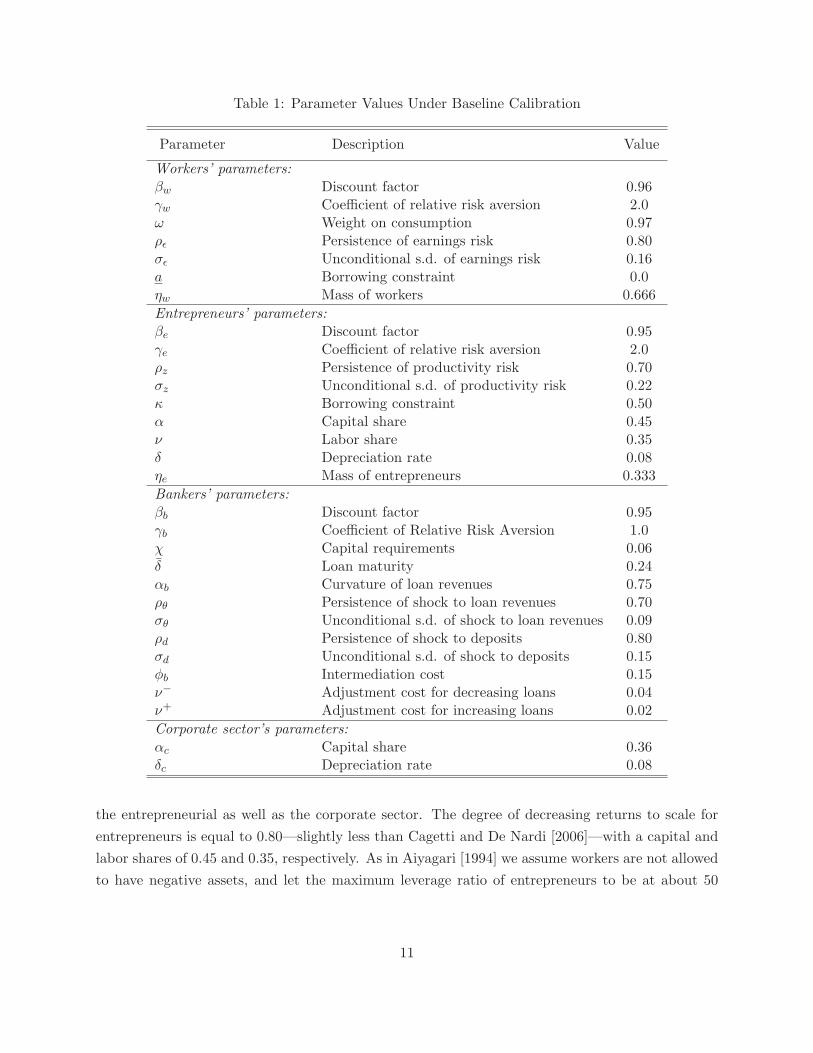
Table 1: Parameter Values Under Baseline Calibration
Parameter Description Value
Workers’ parameters:βw Discount factor 0.96γw Coefficient of relative risk aversion 2.0ω Weight on consumption 0.97ρǫ Persistence of earnings risk 0.80σǫ Unconditional s.d. of earnings risk 0.16a Borrowing constraint 0.0ηw Mass of workers 0.666
Entrepreneurs’ parameters:βe Discount factor 0.95γe Coefficient of relative risk aversion 2.0ρz Persistence of productivity risk 0.70σz Unconditional s.d. of productivity risk 0.22κ Borrowing constraint 0.50α Capital share 0.45ν Labor share 0.35δ Depreciation rate 0.08ηe Mass of entrepreneurs 0.333
Bankers’ parameters:βb Discount factor 0.95γb Coefficient of Relative Risk Aversion 1.0χ Capital requirements 0.06δ Loan maturity 0.24αb Curvature of loan revenues 0.75ρθ Persistence of shock to loan revenues 0.70σθ Unconditional s.d. of shock to loan revenues 0.09ρd Persistence of shock to deposits 0.80σd Unconditional s.d. of shock to deposits 0.15φb Intermediation cost 0.15ν− Adjustment cost for decreasing loans 0.04ν+ Adjustment cost for increasing loans 0.02
Corporate sector’s parameters:αc Capital share 0.36δc Depreciation rate 0.08
the entrepreneurial as well as the corporate sector. The degree of decreasing returns to scale for
entrepreneurs is equal to 0.80—slightly less than Cagetti and De Nardi [2006]—with a capital and
labor shares of 0.45 and 0.35, respectively. As in Aiyagari [1994] we assume workers are not allowed
to have negative assets, and let the maximum leverage ratio of entrepreneurs to be at about 50
11

Table 2: Selected Moments
Moment Data Model
Tier 1 capital ratio 9.3 12.4Share of constrained banks 0.2 0.3Leverage ratio 6.9 7.7Adjusted return-on-assets 3.4 6.0Cross-sectional volatility of adjusted return-on-assets 1.3 1.3% Safe assets held by banks 30.8 38.4Share of interest income in revenues 0.7 0.2Share of noninterest expenses 2.9 9.2Return on securities 2.4 3.3
Loan rate 4.6 4.2Consumption to output 0.7 0.7Banking assets to output 0.7 0.6Safe-to-total assets 0.3 0.3
Memo: Deposit rate 0.6 0.6
% Labor in entrepreneurial sector — 37.6% Labor in corporate sector — 62.4% Output of entrepreneurial sector — 48.6% Output of corporate sector — 44.0% Output of banking sector — 7.5
Note: Moments are based on sample averages using quarterly observations between 1997:Q1 and 2012:Q3,with the exception of the percentage of safe assets held by banks which is only available starting in 2001:Q1,and averages for share of interest income in revenues and banking assets to output are calculated only for theperiod after the fourth quarter of 2008 when investment banks became bank holding companies. The adjustedreturn on assets is defined as net income excluding income taxes and salaries and employee benefits. Thepercentage of safe assets held by banks includes all assets with a zero and with a 20 percent risk weight. Thesample includes all bank holding companies and commercial banks that are not part of a BHC, or that are partof a BHC which does not file the Y-9C report. The share of constrained banks is based on banks’ responses inthe Senior Loan Officer Opinion Survey. The safe-asset share is obtained from Gorton, Lewellen, and Metrick[2012].
percent, which corresponds to κ set to 0.5.9
The discount factor of entrepreneurs is chosen to match the average loan rate between 1997 and
2012. Based on bank holding company and call report data the weighted average real interest rate
charged on loans of all types was 4.6 percent. By setting βe to 0.95 we obtain approximately this
calibration.
Bankers’ problem. We divide the set of parameters of the bankers’ problem into two parts:
(i) parameters set externally, and (ii) parameters set internally. The parameters set externally
are taken directly from outside sources. These include the loan maturity, δ, and the capital con-
9Leverage is defined as debt to assets, that is −b/k. At the constraint b = −κk, the maximum leverage in themodel is equal to κ = 0.50.
12

straint parameter, χ. In addition, we assume the banker has log utility to minimize the amount of
precautionary savings induced by the occasionally binding capital constraint. The remaining nine
parameters of the banker’s problem are determined so that a set of nine moments in the model are
close to a set of nine moments available in the bank holding company and commercial bank call
reports. The lower panel in Table 1 reports the parameter values assumed in the parametrization
of the banker’s problem.
We now describe the parameters set externally. For the capital constraint we assume that the
minimum capital requirement in the model is equal to 6 percent, which corresponds to the minimum
tier 1 ratio a bank must maintain to be considered well capitalized. Thus, χ equals 0.06. The loan
maturity parameter, δ, is set to 0.24 so that the average maturity of loans is 4.2 years based on the
maturity buckets available on banks’ Call Reports.
The parameters set internally—namely the banker’s discount factor, the intermediation cost,
the parameters of the banker’s loan technology, the persistence and standard deviation of the shock
to deposits, and the adjustment cost parameters—are chosen to match a set of nine moments
calculated from regulatory reports. The moments selected are: (i) tier 1 capital ratio, (ii) the
fraction of capital constrained banks, (iii) leverage ratio, (iv) adjusted return-on-assets, (v) the
cross-sectional volatility of adjusted return on assets, (vi) the share of assets with a zero or 20
percent Basel I risk-weight, (vii) the share of interest income relative to total revenues, (viii) the
share of noninterest expenses, and (ix) the return on securities. The upper panel of Table 2 presents
a comparison between the data and the model for this selected set of moments.
As discussed above, the supplies of certain types of safe assets such as U.S. Treasury securities,
Agency debt and municipal bonds are not directly modeled in our framework. We capture the
supply of these assets using the parameter S. As shown in Section 4, our results are somewhat
sensitive to the choice of this parameter. Thus, we calibrate the parameter S using the estimates of
the share of safe assets provided by Gorton, Lewellen, and Metrick [2012]. Specifically, that paper
estimates that during the postwar period the safe-asset share has fluctuated between 30 and 35
percent. In the model we define the safe-asset share as follows. The numerator includes bank
deposits, the exogenous amount of safe assets, S, and the amount of borrowing by banks in the
securities market. The denominator includes all assets in the economy for each of the three types
of agents: workers’ deposits and corporate sector assets; entrepreneurs’ capital and securities; and
bankers’ loans and securities. By setting S to 9, we obtain a safe-asset share of 33 percent in our
calibrated model. The solution of the model is obtained via computational methods and additional
details are provided in the Appendix.
4 Analysis of the Baseline Economy
We first present results for a partial equilibrium version of the model, in which prices (interest rates
and wages) are taken as given, in order to gain intuition regarding the different constraints of the
13
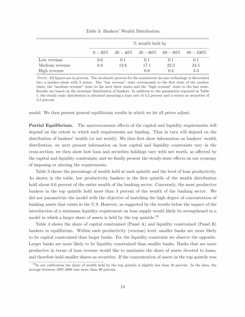
Table 3: Bankers’ Wealth Distribution
% wealth held by
0− 20% 20− 40% 40− 60% 60− 80% 80− 100%
Low revenue 0.6 0.1 0.1 0.1 0.1Medium revenue 8.8 12.6 17.1 22.3 34.5High revenue – – 0.0 0.4 3.3
Note: All figures are in percent. The stochastic process for the noninterest income technology is discretizedinto a markov-chain with 5 states. The “low revenue” state corresponds to the first state of the markovchain, the “medium revenue” state to the next three states and the “high revenue” state to the last state.Results are based on the invariant distribution of bankers. In addition to the parameters reported in Table1, the steady state distribution is obtained assuming a loan rate of 4.2 percent and a return on securities of3.3 percent.
model. We then present general equilibrium results in which we let all prices adjust.
Partial Equilibrium. The macroeconomic effects of the capital and liquidity requirements will
depend on the extent to which such requirements are binding. That in turn will depend on the
distribution of bankers’ wealth (or net worth). We thus first show information on bankers’ wealth
distribution; we next present information on how capital and liquidity constraints vary in the
cross-section; we then show how loan and securities holdings vary with net worth, as affected by
the capital and liquidity constraints; and we finally present the steady-state effects on our economy
of imposing or altering the requirements.
Table 3 shows the percentage of wealth held at each quintile and the level of loan productivity.
As shown in the table, low productivity bankers in the first quintile of the wealth distribution
hold about 0.6 percent of the entire wealth of the banking sector. Conversely, the most productive
bankers in the top quintile hold more than 3 percent of the wealth of the banking sector. We
did not parametrize the model with the objective of matching the high degree of concentration of
banking assets that exists in the U.S. However, as suggested by the results below the impact of the
introduction of a minimum liquidity requirement on loan supply would likely be strengthened in a
model in which a larger share of assets is held by the top quintile.10
Table 4 shows the share of capital constrained (Panel A) and liquidity constrained (Panel B)
bankers in equilibrium. Within each productivity (revenue) level, smaller banks are more likely
to be capital constrained than larger banks. For the liquidity constraint we observe the opposite.
Larger banks are more likely to be liquidity constrained than smaller banks. Banks that are more
productive in terms of loan revenue would like to maximize the share of assets devoted to loans,
and therefore hold smaller shares as securities. If the concentration of assets in the top quintile was
10In our calibration the share of wealth held by the top quintile is slightly less than 40 percent. In the data, theaverage between 1997-2006 was more than 90 percent.
14
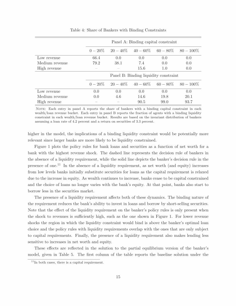
Table 4: Share of Bankers with Binding Constraints
Panel A: Binding capital constraint
0− 20% 20− 40% 40− 60% 60− 80% 80− 100%
Low revenue 66.4 0.0 0.0 0.0 0.0Medium revenue 79.2 38.1 7.4 0.0 0.0High revenue – – 15.6 1.0 0.0
Panel B: Binding liquidity constraint
0− 20% 20− 40% 40− 60% 60− 80% 80− 100%
Low revenue 0.0 0.0 0.0 0.0 0.0Medium revenue 0.0 4.6 14.6 19.8 20.1High revenue – – 90.5 99.0 93.7
Note: Each entry in panel A reports the share of bankers with a binding capital constraint in eachwealth/loan revenue bucket. Each entry in panel B reports the fraction of agents with a binding liquidityconstraint in each wealth/loan revenue bucket. Results are based on the invariant distribution of bankersassuming a loan rate of 4.2 percent and a return on securities of 3.3 percent.
higher in the model, the implications of a binding liquidity constraint would be potentially more
relevant since larger banks are more likely to be liquidity constrained.
Figure 1 plots the policy rules for bank loans and securities as a function of net worth for a
bank with the highest revenue shock. The dashed line represents the decision rule of bankers in
the absence of a liquidity requirement, while the solid line depicts the banker’s decision rule in the
presence of one.11 In the absence of a liquidity requirement, as net worth (and equity) increases
from low levels banks initially substitute securities for loans as the capital requirement is relaxed
due to the increase in equity. As wealth continues to increase, banks cease to be capital constrained
and the choice of loans no longer varies with the bank’s equity. At that point, banks also start to
borrow less in the securities market.
The presence of a liquidity requirement affects both of these dynamics. The binding nature of
the requirement reduces the bank’s ability to invest in loans and borrow by short-selling securities.
Note that the effect of the liquidity requirement on the banker’s policy rules is only present when
the shock to revenues is sufficiently high, such as the one shown in Figure 1. For lower revenue
shocks the region in which the liquidity constraint would bind is above the banker’s optimal loan
choice and the policy rules with liquidity requirements overlap with the ones that are only subject
to capital requirements. Finally, the presence of a liquidity requirement also makes lending less
sensitive to increases in net worth and equity.
These effects are reflected in the solution to the partial equilibrium version of the banker’s
model, given in Table 5. The first column of the table reports the baseline solution under the
11In both cases, there is a capital requirement.
15

Figure 1: The Effect of the LCR constraint on bankers’ policy rules
100 200 300 400200
250
300
350
400
450
500
550
600
650Loans
Net worth
No LCRLCR
100 200 300 400250
300
350
400
450
500
550
600
650
700Securities
Net worth
Notes: Policy rules for the bankers under the highest revenue state θ = θ5, average level of deposits d = d2and stock of loans l = 140.
presence of a capital requirement, but not a liquidity requirement. The second column reports the
impact of introducing liquidity requirements on model outcomes. The third column reports the
model outcomes in response to an increase in the capital requirement from 6 to 12 percent, and the
last column reports the impact of simultaneously increasing the capital requirement and imposing
a liquidity requirement.
The introduction of a liquidity requirement (second column) leads to a substantial increase in
the stock of securities and a decrease in the stock of loans, leaving total assets about flat. Although
banks’ equity fall somewhat, the more substantial decline in loans boosts the aggregate capital
ratio. Though the liquidity requirement only binds for a relatively small share of banks, since these
16

Table 5: Partial Equilibrium Analysis of the Banking Sector
Baseline ∆’s relative to Baseline
Capital requirements 6% 6% 12% 12%
Liquidity requirements No Yes No Yes
(1) (2) (3) (4)
1. Securities 10.2% 11.2% 18.1%
2. Loans -5.8% -2.4% -6.6%
3. Assets (=1+2) 0.3% 2.8% 2.9%
4. Equity 3.9% 37.3% 38.2%
5. Liquidity coverage ratio (%) 150.1 158.8 161.3 167.2
6. Liquidity constraint binds (%) — 12.9 — 12.0
7. Capital ratio (%) 12.2 13.5 17.2 18.1
8. Capital constraint binds (%) 26.4 22.0 36.1 32.6
Note: Results are based on the invariant distribution of bankers. The baseline economy is one in whichcapital requirements are equal to 6 percent (χ = 0.06) and there are no liquidity requirements. The rate onloans and the return on securities are set at 3.6 and 1.6 percent, respectively.
are the largest banks in our model the effect of imposing a liquidity requirement is quite significant.
An increase in capital requirements from 6 to 12 percent (third column) would increase the stock
of equity at banks by more than 35 percent, decrease loans over 2 percent, and increase securities
holdings by about 11 percent. Higher capital requirements make it more difficult for bankers’ to
smooth consumption, thereby increasing the demand to purchase securities which are riskless.
The last column of Table 5 combines the increase in capital and liquidity requirements. The
overall net impact on equity is positive and both the capital ratio and the liquidity coverage ratio
increase significantly relative to the baseline specification. The balance sheet size of banks expands
modestly, while loans shrink and securities holdings increase substantially.
General Equilibrium. The first column of Table 6 reports the baseline general equilibrium solu-
tion of the full model without a liquidity requirement. In general equilibrium prices (RL, RS , R, w)
have to adjust to clear the loan, securities, the asset and the labor markets. In addition, we will be
able to make statements about aggregate consumption and output.
The second column of Table 6 reports the impact on banking and macroeconomic variables in
response to the introduction of a liquidity standard. Securities, loans, assets and equities (rows
1-3 and 5) behave similarly to the partial equilibrium case, though the magnitudes are attenuated.
This reduction in magnitude comes from the impact of changes in the loan rate and the return
17
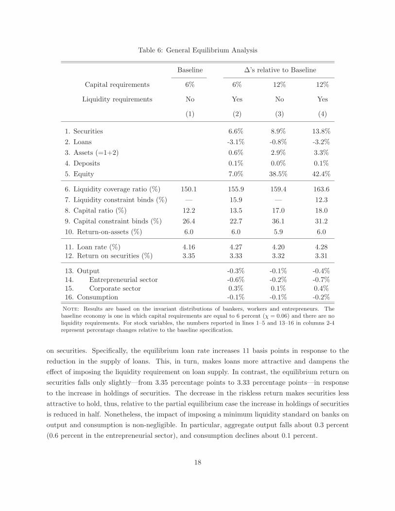
Table 6: General Equilibrium Analysis
Baseline ∆’s relative to Baseline
Capital requirements 6% 6% 12% 12%
Liquidity requirements No Yes No Yes
(1) (2) (3) (4)
1. Securities 6.6% 8.9% 13.8%
2. Loans -3.1% -0.8% -3.2%
3. Assets (=1+2) 0.6% 2.9% 3.3%
4. Deposits 0.1% 0.0% 0.1%
5. Equity 7.0% 38.5% 42.4%
6. Liquidity coverage ratio (%) 150.1 155.9 159.4 163.6
7. Liquidity constraint binds (%) — 15.9 — 12.3
8. Capital ratio (%) 12.2 13.5 17.0 18.0
9. Capital constraint binds (%) 26.4 22.7 36.1 31.2
10. Return-on-assets (%) 6.0 6.0 5.9 6.0
11. Loan rate (%) 4.16 4.27 4.20 4.2812. Return on securities (%) 3.35 3.33 3.32 3.31
13. Output -0.3% -0.1% -0.4%14. Entrepreneurial sector -0.6% -0.2% -0.7%15. Corporate sector 0.3% 0.1% 0.4%16. Consumption -0.1% -0.1% -0.2%
Note: Results are based on the invariant distributions of bankers, workers and entrepreneurs. Thebaseline economy is one in which capital requirements are equal to 6 percent (χ = 0.06) and there are noliquidity requirements. For stock variables, the numbers reported in lines 1–5 and 13–16 in columns 2-4represent percentage changes relative to the baseline specification.
on securities. Specifically, the equilibrium loan rate increases 11 basis points in response to the
reduction in the supply of loans. This, in turn, makes loans more attractive and dampens the
effect of imposing the liquidity requirement on loan supply. In contrast, the equilibrium return on
securities falls only slightly—from 3.35 percentage points to 3.33 percentage points—in response
to the increase in holdings of securities. The decrease in the riskless return makes securities less
attractive to hold, thus, relative to the partial equilibrium case the increase in holdings of securities
is reduced in half. Nonetheless, the impact of imposing a minimum liquidity standard on banks on
output and consumption is non-negligible. In particular, aggregate output falls about 0.3 percent
(0.6 percent in the entrepreneurial sector), and consumption declines about 0.1 percent.
18

The third column of Table 6 reports the general equilibrium results when capital requirements
increase from 6 to 12 percent. In this case the results are also less pronounced relative to the partial
equilibrium case. Specifically, loans decline less than 1 percent, while securities increase somewhat
less relative to the partial equilibrium case. In large part, the increase in demand for securities
leads to a small reduction in the equilibrium rate of return on securities (row 12). Although the
new steady state level of aggregate output is about flat in response to the increase in capital
requirements, consumption still falls in large part because banks need to pay less dividends to
sustain the higher capital ratios.
Finally, the last column in Table 6 reports the combined effects of an increase in capital and
liquidity requirements. The model suggests that a simultaneous increase in capital and liquidity
requirements would cause output and consumption to both decline by about 0.4 and 0.2 percent,
respectively. Although the decline in output is somewhat modest, there is a sizable redistribution
effect of the economy’s production capacity from entrepreneurs (bank dependent borrowers) to the
corporate sector.
Supply of Safe Assets. We now analyze the comparative statics in our economy when the
supply of safe assets—controlled by the parameter S—increases. The availability of safe assets has
important implications for the liquidity requirement in our model—as defined in equation (3)—
since banks are required to invest a share of their liabilities in liquid assets. In our calibration,
the parameter S represents the “exogenous” amount of safe assets available in our economy. This
parameter represents liquid assets available in the economy that are not explicitly modeled in our
framework, such as debt securities that have the explicit or implicit backing of the U.S. Government
or central bank reserves than can be drawn in time of stress. Therefore, it is important to understand
how the equilibrium changes in response to an exogenous variation in the supply of safe assets and
for reasons not related to the introduction of a liquidity requirement in the banking sector.
The left panel of Figure 2 plots the steady state equilibrium in the securities market before the
introduction of the liquidity requirement. The supply of securities is positively sloped (the blue
line) and corresponds to the sum of an exogenous component—defined by the parameter S—and an
endogenous component determined by banks that are supplying safe assets to the market (i.e., those
with s′ < 0). The demand for securities by bankers and entrepreneurs is represented by the red
solid line and is negatively sloped. The equilibrium in the securities market before the introduction
of a liquidity requirement is represented by the dot labeled ‘A’ in the left panel. The dashed lines
represent the supply and demand of securities after the introduction of the liquidity requirement.
As shown by the blue lines in the left panel, the introduction of the liquidity requirement shifts the
supply curve to the left and makes it very inelastic. This happens because one way for banks to ease
the liquidity requirement constraint is to reduce their amount of borrowing in the securities’ market,
making the supply of securities almost exclusively determined by the parameter S. Meanwhile, the
demand for securities remains about unchanged because an increase in banks’ demand for securities
19
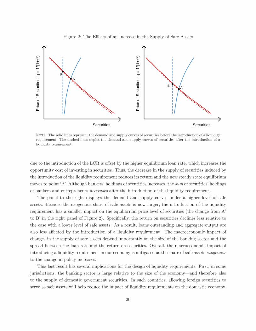
Figure 2: The Effects of an Increase in the Supply of Safe AssetsP
rice
of S
ecur
ities
, q =
1/(
1+r
)s
Securities
AB
Pric
e of
Sec
uriti
es, q
= 1
/(1+
r )s
Securities
A’B’
Note: The solid lines represent the demand and supply curves of securities before the introduction of a liquidityrequirement. The dashed lines depict the demand and supply curves of securities after the introduction of aliquidity requirement.
due to the introduction of the LCR is offset by the higher equilibrium loan rate, which increases the
opportunity cost of investing in securities. Thus, the decrease in the supply of securities induced by
the introduction of the liquidity requirement reduces its return and the new steady state equilibrium
moves to point ‘B’. Although bankers’ holdings of securities increases, the sum of securities’ holdings
of bankers and entrepreneurs decreases after the introduction of the liquidity requirement.
The panel to the right displays the demand and supply curves under a higher level of safe
assets. Because the exogenous share of safe assets is now larger, the introduction of the liquidity
requirement has a smaller impact on the equilibrium price level of securities (the change from A’
to B’ in the right panel of Figure 2). Specifically, the return on securities declines less relative to
the case with a lower level of safe assets. As a result, loans outstanding and aggregate output are
also less affected by the introduction of a liquidity requirement. The macroeconomic impact of
changes in the supply of safe assets depend importantly on the size of the banking sector and the
spread between the loan rate and the return on securities. Overall, the macroeconomic impact of
introducing a liquidity requirement in our economy is mitigated as the share of safe assets exogenous
to the change in policy increases.
This last result has several implications for the design of liquidity requirements. First, in some
jurisdictions, the banking sector is large relative to the size of the economy—and therefore also
to the supply of domestic government securities. In such countries, allowing foreign securities to
serve as safe assets will help reduce the impact of liquidity requirements on the domestic economy.
20

Second, reserves held at the central bank can serve as a potentially large source of safe assets.
A number of central banks have greatly increased the supply of such reserves as a consequence
of running nontraditional monetary policies at the zero lower bound. Because having a large
quantity of reserves can mitigate the macroeconomic effects of introducing a liquidity requirement,
maintaining reserves at a high level through the transition period of introducing the requirement
may be beneficial.
5 Transitional Dynamics
In this section, we illustrate the transitional dynamics of introducing liquidity requirements and
compare those to the responses to an increase in capital requirements. In contrast to the results of
the previous section, we assume a gradual increase in the liquidity requirement over a three year
horizon and describe the responses of all sectors in our economy. In addition, we also compare
these responses to the case in which the increase in capital requirements is also done gradually over
a three year horizon.
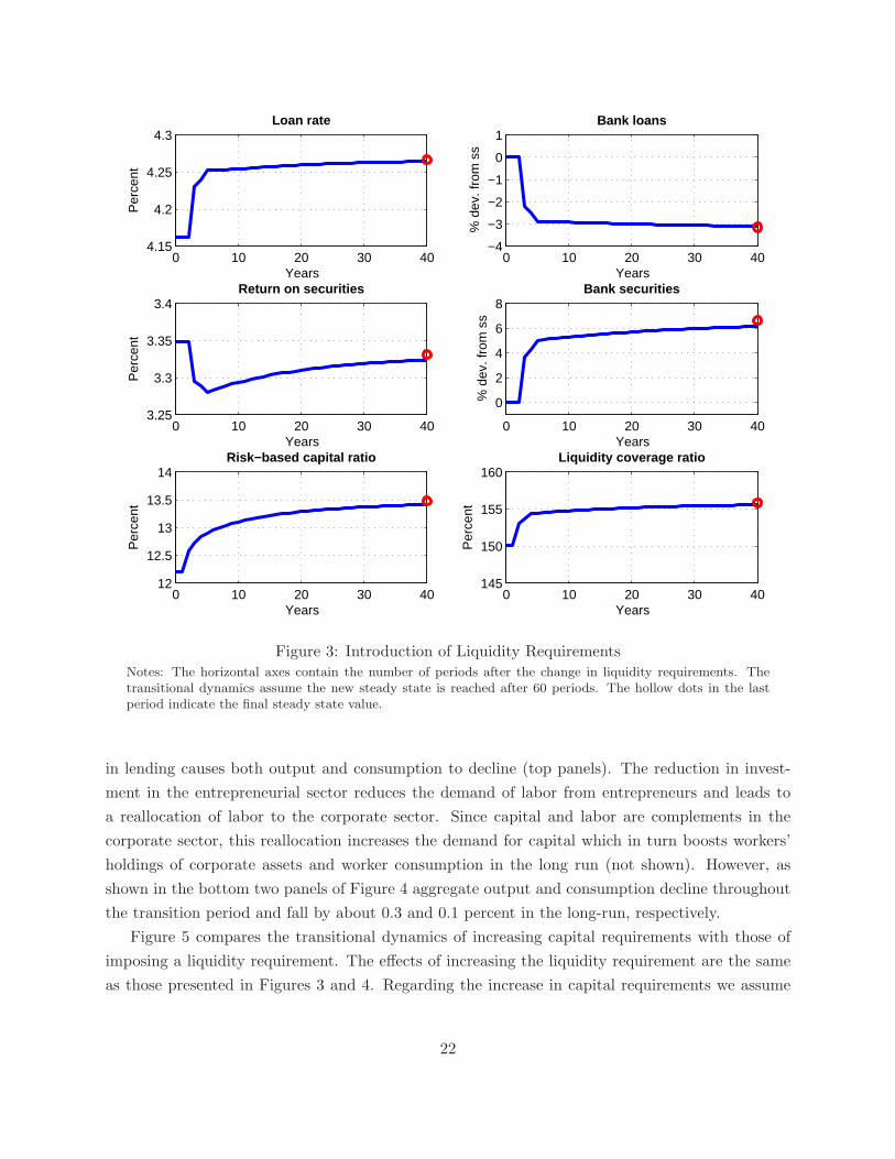
Introduction of a liquidity requirement. Figure 3 shows the transitional dynamics of the
banking sector in response to the introduction of a liquidity standard. The liquidity standard is
increased gradually over a three-year horizon and mimics the transition period under the U.S. LCR
proposal.12 Specifically, we assume that in period 1 the economy is in its steady state equilibrium.
In period 2, an unanticipated liquidity requirement is announced and implemented at 80 percent,
followed by 90 percent in period 3 and reaching 100 percent in period 4. The computational
method used to calculate the transitional dynamics is presented in the Appendix. Bankers respond
to the introduction of a liquidity standard by decreasing the supply of loans (top right panel) and
increasing their holdings of securities (middle right panel). This triggers an increase in the loan
rate of approximately 10 basis points in the long run (top left panel) and a decrease in the return of
securities of a similar magnitude (middle left panel). The shift in portfolio composition of bankers
from loans to securities increases the liquidity coverage ratio (bottom right panel) and also boosts
their risk-based capital ratio (bottom left panel). The increase in banks’ risk-based capital ratios
is driven in part by the zero risk-weighting of securities. In addition, the liquidity requirement also
penalizes banks’ dependence on deposits and borrowing in the securities’ market and as a result it
increases their desire to finance with retained earnings.
Figure 4 displays the responses of entrepreneurial and aggregate output and consumption. On
the entrepreneurial sector, the introduction of the liquidity requirement and subsequent reduction
12October 24, 2013, U.S. regulatory agencies proposed a LCR that would apply to bank holding companies with$250 billion or more in total consolidated assets or $10 billion or more in on-balance-sheet foreign exposure. Theproposed LCR establishes a transition period beginning January 1, 2015 with an 80 percent LCR requirement, 90percent by January 2016 and 100 percent by January 2017.
21
0 10 20 30 404.15
4.2
4.25
4.3Loan rate
Years
Per
cent
0 10 20 30 40−4
−3
−2
−1
0
1Bank loans
% d
ev. f
rom
ss
Years
0 10 20 30 403.25
3.3
3.35
3.4Return on securities
Per
cent
Years0 10 20 30 40
0
2
4
6
8Bank securities
% d
ev. f
rom
ss
Years
0 10 20 30 4012
12.5
13
13.5
14Risk−based capital ratio
Per
cent
Years0 10 20 30 40
145
150
155
160Liquidity coverage ratio
Per
cent
Years
Figure 3: Introduction of Liquidity RequirementsNotes: The horizontal axes contain the number of periods after the change in liquidity requirements. Thetransitional dynamics assume the new steady state is reached after 60 periods. The hollow dots in the lastperiod indicate the final steady state value.
in lending causes both output and consumption to decline (top panels). The reduction in invest-
ment in the entrepreneurial sector reduces the demand of labor from entrepreneurs and leads to
a reallocation of labor to the corporate sector. Since capital and labor are complements in the
corporate sector, this reallocation increases the demand for capital which in turn boosts workers’
holdings of corporate assets and worker consumption in the long run (not shown). However, as
shown in the bottom two panels of Figure 4 aggregate output and consumption decline throughout
the transition period and fall by about 0.3 and 0.1 percent in the long-run, respectively.
Figure 5 compares the transitional dynamics of increasing capital requirements with those of
imposing a liquidity requirement. The effects of increasing the liquidity requirement are the same
as those presented in Figures 3 and 4. Regarding the increase in capital requirements we assume
22

0 10 20 30 40
−0.5
−0.4
−0.3
−0.2
−0.1
0
0.1Entrepreneurial output
% d
ev. f
rom
ss
Years0 10 20 30 40
−0.4
−0.3
−0.2
−0.1
0
0.1Entrepreneurial consumption
% d
ev. f
rom
ss
Years
0 10 20 30 40−0.4
−0.3
−0.2
−0.1
0
Aggregate output
% d
ev. f
rom
ss
Years0 10 20 30 40
−0.1
−0.05
0
0.05Aggregate consumption
% d
ev. f
rom
ss
Years
Figure 4: Introduction of Liquidity RequirementsNotes: The horizontal axes contain the number of periods after the change in liquidity requirements. Thetransitional dynamics assume the new steady state is reached after 60 periods. The hollow dots in the lastperiod indicate the final steady state value.
those are unanticipated and rise from 6 to 12 percent over three periods. The effects from imposing
a higher capital requirement are different from those of introducing a liquidity requirement since
the capital and liquidity constraints bind for a different set of banks and it operates through a
different mechanism. Specifically, an increase in capital requirements implies that, for a given level
of profitability risk, it becomes harder to smooth dividend payouts for bankers. As a result, bankers
would like to accumulate more securities (precautionary buffer) and would substitute out of loans
into securities. In general equilibrium, bankers’ portfolio reallocation leads to a decrease in the rate
of return of securities and an increase in the rate of return of loans.
Under our calibration, we find that in response to the increase in capital requirements loan
rates increase close to 15 basis points in the near term but subsequently rebound to their baseline
23

value (top left panel). Similarly, outstanding loans on banks’ books fall about 4 percent in the
short term but are little changed in the long-run (top right panel). In response to higher capital
requirements, the most affected banks are the ones with the lowest levels of equity and the least
profitable. As a result, the increase in capital requirements increases their precautionary desire
to hold securities which leads to a substantial decrease in the return on those assets (not shown).
Consequently, loans become relatively more attractive for banks, offsetting the initial negative effect
on lending. In addition, since the supply of loans to bank dependent borrowers is little changed
the long-run effects of increasing capital requirements on aggregate output and consumption are
relatively small (bottom panels).
Comparing effects of imposing liquidity requirements with increasing capital require-
ments. Figure 5 shows that the evolution of the variables of the model along the transition path
are different across the two experiments of imposing a liquidity standard and increasing capital
requirements. In the case of the introduction of liquidity requirement, the affected banks are the
largest and most profitable. Because banks most affected by the liquidity requirement are not
capital constrained, the decline in bank loans in the long run is more pronounced when liquidity
requirements are imposed due to the lack of banks’ demand to hold additional assets to minimize
fluctuations in dividend payouts in response to idiosyncratic revenue shocks. Moreover, the increase
in capital requirements leads to a higher increase in banks’ liquidity coverage ratios. According to
our model, policy makers would be able to increase banks’ holdings of liquid assets more quickly
by increasing capital requirements rather than imposing a liquidity requirement (middle panels).
We are able to obtain this result in the model because liquid assets have lower risk-weights than
loans, which is consistent with what is typically observed in the data.
Interestingly, the decline in aggregate consumption in the short-term is considerably more pro-
nounced in the case of more stringent capital requirements as banks accumulate equity by reducing
dividend payouts to meet the higher capital requirement (bottom right panel).
Sensitivity analysis. As shown in Table 6, the LCR is about 150 percent in the baseline economy.
To generate this ratio the model implicitly assumes a 60 percent run-off rate for deposits during a
liquidity stress event, which is higher than what is assumed under the U.S. LCR rules. That said,
anecdotal evidence based on banks’ earnings reports suggest that banks’ liquidity coverage ratios
are between 80 and 120 percent in recent quarters; that is, significantly lower than the aggregate
LCR we obtain in our baseline economy. Thus, it is plausible to assume that the LCR ratio
generated in the baseline calibration is simply too high, suggesting that the liquidity requirements
are unrealistically low in the model. In addition, the results of the comprehensive quantitative
impact study BCBS [2010b], estimate that the liquidity coverage ratio for the set of banks included
24

0 10 20 30 404.1
4.15
4.2
4.25
4.3Loan rate
Years
Per
cent
LCRHigher capital
0 10 20 30 40
−4
−2
0
Bank loans
% d
ev. f
rom
ss
Years
0 10 20 30 40
12
14
16
18Risk−based capital
Per
cent
Years0 10 20 30 40
145
150
155
160
165Liquidity coverage ratio
Per
cent
Years
0 10 20 30 40−0.4
−0.3
−0.2
−0.1
0
0.1Aggregate output
% d
ev. f
rom
ss
Years0 10 20 30 40
−0.4
−0.3
−0.2
−0.1
0
0.1Aggregate consumption
% d
ev. f
rom
ss
Years
Figure 5: Comparison of Introducing Liquidity Requirements with Increasing CapitalRequirements
Notes: The horizontal axes contain the number of periods after the change in liquidity or capital requirements.The transitional dynamics assume the new steady state is reached after 60 periods.
in their sample was 83 percent for Group 1 banks.13
There are a few reasons supporting the idea that under our baseline calibration liquidity re-
quirements are too loose. First, we do not accurately model loan commitments, since bank loans by
entrepreneurs in the model are fully drawn at origination. According to Santos [2011], the average
drawdown rate for non-financial borrowers is about 23 percent over a one year-horizon; drawdowns
are significantly higher during recessions and financial crises. As a result, we could model draw-
downs of credit facilities during a stress period by also including an outflow assumption on loans
to entrepreneurs.
13Group 1 banks are those that have Tier 1 capital in excess of 3 billion of euros, are well diversified, and areinternationally active. Of the 91 Group 1 banks included in the quantitative impact study, 13 were U.S. banks.
25

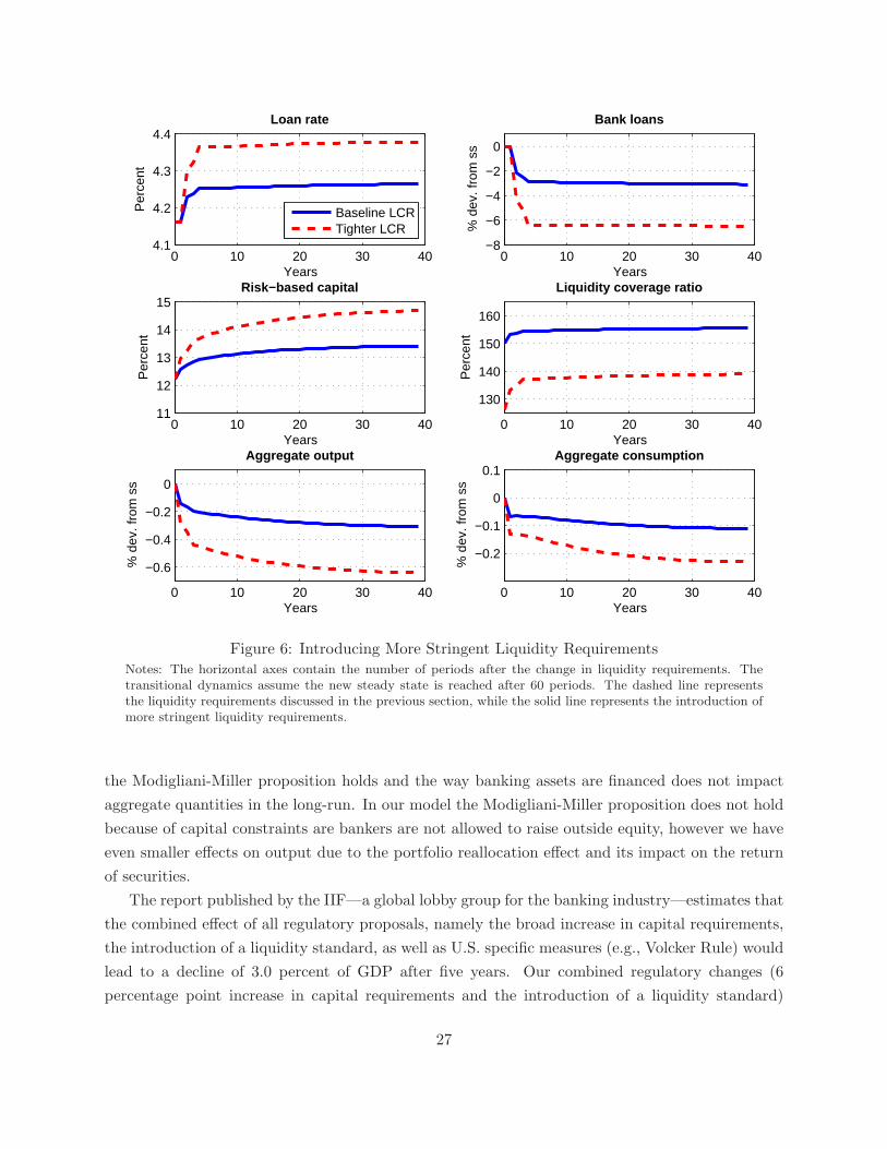
Figure 6 depicts the responses of the variables of the model under different parametrizations of
the liquidity standard. In particular, the red dashed lines show the evolution of the variables in the
model corresponding to a liquidity coverage ratio of 125 percent in the baseline economy. To attain
this calibration we lowered the parameter that controls paydowns on existing loans, δ, from 0.24 to
0.10. Relative to the solid blue line, which represents the baseline change in the liquidity standard,
the loan rate increases about 20 basis points in the long-run instead of 10 basis points (top left
panel). Similarly, holdings of loans on banks’ books declines about 6 percent (top right panel).
Aggregate output in the long-run declines by 0.6 percent (bottom left panel). Clearly, increasing
the cash outflow assumptions over the stress period would lead to a greater impact of imposing a
liquidity standard in the macroeconomy.
Discussion. Our model induces a positive correlation between loan revenue and bank size. As
shown in Table 4, the liquidity requirement is more likely to bind for larger banks than smaller
ones. Because there is a significant concentration of assets among the largest banks, they have a
large influence on total loans outstanding in our economy. For this reason, we expect to find a
stronger impact of changes in liquidity requirements on the evolution of macroeconomic variables
relative to a setup with a representative bank.
In addition, the effect of the introduction of liquidity requirements on aggregate output is
permanent. This occurs because the liquidity requirement prevents the most productive banks
from fully exploiting their profitable opportunities, and the introduction of a liquidity requirement
does not lead to a material reduction in the cost of funds to the bank. However, our model only
allows for one form of debt finance subject to the same liquidity requirement. If banks have access
to other sources of debt finance with longer maturities which are exempted from the liquidity
requirement, or have lower outflows assumptions, the impact on loan growth could be mitigated.
Discussion of other estimates on the impact of regulatory reform. There are two well-
known studies on the macroeconomic impact of the regulatory reform that are helpful to summarize.
First, the Macroeconomic Assessment Group (MAG) produced a reported published by the BCBS
[2010a] at the end of 2010. Second, the Institute of International Finance IIF [2011]—representatives
for the banking industry—publishes a report every year on the macroeconomic impact of regulatory
reforms, which was last updated in August of 2013. In the MAG report, it is estimated that a one
percentage point increase in minimum capital requirements leads to a decline of 0.19 percent of
output relative to the baseline in almost five years. Assuming we can scale up the MAG estimate,
then a six percentage point increase in capital requirements leads to a 1.2 percent decrease in
output over the same period. The contraction in output provided by the MAG analysis is signif-
icantly larger than the estimate suggested by our model. In particular, our calibration suggests
that a six percentage point increase in capital requirements leads to a decline of 0.1 percent in
aggregate output after 5 years. In the MAG study, the results are based on the assumption that
26
0 10 20 30 404.1
4.2
4.3
4.4Loan rate
Years
Per
cent
Baseline LCRTighter LCR
0 10 20 30 40−8
−6
−4
−2
0
Bank loans
% d
ev. f
rom
ss
Years
0 10 20 30 4011
12
13
14
15Risk−based capital
Per
cent
Years0 10 20 30 40
130
140
150
160
Liquidity coverage ratio
Per
cent
Years
0 10 20 30 40
−0.6
−0.4
−0.2
0
Aggregate output
% d
ev. f
rom
ss
Years0 10 20 30 40
−0.2
−0.1
0
0.1Aggregate consumption
% d
ev. f
rom
ss
Years
Figure 6: Introducing More Stringent Liquidity RequirementsNotes: The horizontal axes contain the number of periods after the change in liquidity requirements. Thetransitional dynamics assume the new steady state is reached after 60 periods. The dashed line representsthe liquidity requirements discussed in the previous section, while the solid line represents the introduction ofmore stringent liquidity requirements.
the Modigliani-Miller proposition holds and the way banking assets are financed does not impact
aggregate quantities in the long-run. In our model the Modigliani-Miller proposition does not hold
because of capital constraints are bankers are not allowed to raise outside equity, however we have
even smaller effects on output due to the portfolio reallocation effect and its impact on the return
of securities.
The report published by the IIF—a global lobby group for the banking industry—estimates that
the combined effect of all regulatory proposals, namely the broad increase in capital requirements,
the introduction of a liquidity standard, as well as U.S. specific measures (e.g., Volcker Rule) would
lead to a decline of 3.0 percent of GDP after five years. Our combined regulatory changes (6
percentage point increase in capital requirements and the introduction of a liquidity standard)
27
would lead to a decline of 0.4 percent of aggregate output in the long-run. In the IIF study, a key
driving force of the results in the increase in loan spreads. In our model the loan rate also increases
in response to the more stringent regulatory requirements, albeit by much less. Due to the general
equilibrium nature of our model, the bulk of the adjustment occurs through the reallocation of
banks’ portfolios as bank dependent borrowers curtail their demand for funds in response to higher
loan rates. Because the IIF is based on a partial equilibrium analysis, the impact of the regulatory
reform on spreads is probably overstated.
6 Implications for Macroprudential Policy
In this section we evaluate the behavior of our model economy in response to an aggregate shock
to the wealth of workers subject to different macroprudential policy alternatives. During a stress
scenario, regulators may wish to temporarily relax regulations in order to reduce the impact of
shocks on the macroeconomy.14 Specifically, we use our model to compare the effects on output of
easing liquidity standards against a reduction in capital requirements in response to an aggregate
shock. Bank capital stress tests have in recent years become an indispensable part of the toolkit
used by central banks and other regulators to conduct macroprudential regulation and supervision.
Perhaps liquidity stress tests could also become an important instrument in the implementation of
macroprudential regulation.
We introduce an aggregate shock in our economy by considering a one-time, two-period shock to
the distribution of workers’ wealth. Specifically, we shock the distribution of wealth of workers by
5 percent in the first period and 3.3 percent in the second period. In addition, we apply the shock
in the economy that includes both a capital requirement of 12 percent and the liquidity standard
described in equation (3). We consider two types macroprudential policies. The first type relaxes
the capital requirement from 12 to 6 percent in the first three periods after the wealth shock occurs
and then assumes the capital requirement rises gradually to 12 percent over the next four periods.
The macroprudential policy based on the relaxation of the liquidity standard assumes that the
LCR is lifted entirely for the first three periods and then rises gradually to 100 percent during the
remaining four periods. The shock to the wealth of workers in the first two periods is assumed to
be unexpected, but after the shock occurs agents have perfect foresight in terms of both the capital
and liquidity regulation policies.
Figure 7 plots the response of our economy to the one-time shock to the distribution of workers’
wealth. As shown in the baseline case (dash-dotted blue line), aggregate output is 2.1 percent lower
in period 3 after the initial shock in periods 1 and 2. The response in the economy in which capital
requirements are relaxed in the first 6 periods is similar, with aggregate output declining 2 percent
by period 3. In other words, while the easing of capital requirements helps to dampen the response
14For an overview of macroprudential policies, see Hanson, Kashyap, and Stein [2011].
28

−2 0 2 4 6 8 10 12 14−2.5
−2
−1.5
−1
−0.5
0Aggregate output
Years
% d
ev. f
rom
ss
BaselineRelax RBCRelax LCRRelax tighter LCR
Figure 7: Aggregate Response of Output to a Wealth ShockNotes: The horizontal axes contain the number of periods after an aggregate shock that reduces the wealth ofworkers. The transitional dynamics assume the steady state is reached after 60 periods. The dash-dotted blueline represents the response of the economy where capital requirements are 12% and bankers are subject to aliquidity standard, and these standards do not change in response to the wealth shock. The dashed black linerepresents the response of the economy when capital requirements are relaxed temporarily. The pink dashedline represents the response of the economy when liquidity standards are eased temporarily (less stringent)and the red line represents the case where liquidity requirements are more stringent (see text for details).
of output, the effects are fairly small for such a very large reduction in capital requirements. On
the other hand, a relaxation of the liquidity requirement helps to mitigate the decline in aggregate
output a bit more. As shown in the red line, output declines roughly 30 basis points less by period
3 relative to the baseline case in which liquidity requirements are quite stringent before the shock
occurs (LCR of 125).
7 Conclusion
Bank liquidity regulations have the highly desirable goals of both reducing the likelihood of bank
runs and increasing the odds that banks will survive runs, should they occur. However, by increasing
banks’ incentives to hold lower-risk, more liquid assets, such regulations may also reduce the supply
of loans and increase their cost to bank dependent borrowers. They may also interact with other
29

current regulations, such as capital regulations, in ways not completely intended.
In this paper, we calibrate a nonlinear dynamic general equilibrium model in which banks
are subject to both capital and liquidity requirements that bind only occasionally. We find that
imposing liquidity regulations of the kinds currently envisioned under Basel III would, in the long
run, reduce loans outstanding on banks’ books by nearly 3 percent, and aggregate output and
consumption by about 0.3 percent and 0.1 percent, respectively. However, we also find that an
economy with liquidity requirements that could be relaxed during a crisis period could dampen the
effect of wealth shocks on aggregate output relative to an economy in which liquidity requirements
are absent. Thus, introducing liquidity requirements creates an important macroprudential tool
available to policymakers.
We also report that the effects on lending and other banking variables are substantially larger
in partial equilibrium analysis which takes prices as given. This result suggests that attempting
to apply partial equilibrium results—i.e. results just on the banking sector–to derive the macroe-
conomic impact of changes in liquidity or capital regulations are likely to be misleading. But it
also indicates that the macroeconomic impacts of changes in liquidity and capital regulation are
sensitive to the effects of changes in bank behavior on prices. That said, our baseline calibration
suggests a small impact of bank securities purchases on the returns on such securities–which decline
a few basis points after the introduction of a liquidity requirement. The macroeconomic effects of
imposing the liquidity requirement are also smaller the larger the supply of safe assets, suggesting
that it would be desirable to have a large amount of such assets during the proposed transition
period.
Finally, we do not explicitly attempt to model the reduction in bank runs owing to the new
regulations. Thus, our analysis should not be taken as a full evaluation of the costs and benefits
associated with liquidity regulation; nor does it suggest what the optimal level of regulation should
be. We leave that for future research.
30

Appendix
In this appendix we derive the banker’s capital constraints, the first-order conditions of the banker’s
problem, and provide an outline of the solution method.
Banker’s capital constraint. The balance sheet constraint of the banker is given by
b′ + s′ = xb − cb − Φ(b′, δb)− d′
where the left-hand side of this expression is the banker’s assets, b′ + s′, and the right-hand side is
the banker’s equity, eb ≡ xb − cb − Φ(b′, δb), and debt, −d′. The capital constraint can be written
as
eb > χb′
b′ + s′ + d′ > χb′
d′ > (χ− 1)b′ − s′.
Banker’s first-order conditions. The first-order conditions for b′ and s′ are as follows:
[
1 +∂Φ(b′, b)
∂b′
]
uc(c) = βbE
[
∂vb∂xb
∂xb∂b′
+∂vb∂b′
∣
∣
∣
∣
θ, d′]
+ (1− χ)λ+ δµ
uc(c) = βbE
[
∂vb∂xb
∂xb∂s′
∣
∣
∣
∣
θ, d′]
+ λ+ µRS
where λ is the Lagrange multiplier associated with the capital constraint and µ is the Lagrange
multiplier associated with the liquidity constraint. Note that the envelope conditions are
∂vb∂xb
= uc(c)
∂vb∂b
= −uc(c)∂Φ
∂b.
Using the envelope condition on the set of first-order conditions one obtains:
[
1 +∂Φ(b′, b)
∂b′
]
uc(c) = βbE
[(
θ′gb(b′) +RL − φb −
∂Φ(b′′, b′)
∂b′
)
uc(c′)
∣
∣
∣
∣
θ, d′]
+ (1− χ)λ+ δµ
uc(c) = βbE
[
RSuc(c′)
∣
∣
∣
∣
θ, d′]
+ λ+ µRS
Numerical solution. The numerical algorithm solves the banker’s problem by solving for a fixed
point in the consumption function by time iteration as in Coleman [1990]. The policy function
cb(θ, xb, b, d′) is approximated using piecewise bilinear interpolation of the state variables xb and b.
31

The variables xb and b are discretized in a non-uniformly spaced grid points with 100 nodes each.
More grid points are allocated to lower levels of each state variable. The two stochastic processes,
θ and d′, are discretized into five and four states, respectively, using the method proposed by
Tauchen [1986]. The policy functions of consumption for workers and entrepreneurs are also solved
by time iteration. Because the state space is smaller the variables xw and xe are discretized in
a non-uniformly spaced grid with 900 nodes. The invariant distributions of bankers, workers and
entrepreneurs are derived by computing the inverse decision rules on a finer grid than the one
used to compute the optimal decision rules. Finally, the equilibrium prices are determined using a
standard quasi-newton method.
Transitional dynamics. The transition to the new stationary equilibrium is calculated assuming
the new steady state is reached after 60 periods (T = 60). We take as inputs the steady state
distribution of agents in period t = 1 (prior to the change in policy), guesses for the path of RL,
RS , and K/L between t = 1 and t = T , and the optimal decision functions at the new steady state.
Using those guesses we solve the problem of each agent backwards in time, for t = T−1, . . . , 1. With
the time-series sequence of decision rules for each agent we simulate the dynamics of the distribution
for workers, entrepreneurs and bankers and check if the loan market, the deposit market and goods
market clear. If the these markets are not in equilibrium we update the path of RL, RS and K/L
using a simple linear updating rule. Finally, after convergence of the algorithm, we compare the
simulated distribution at T = 60, with the steady state distribution of each agent type obtained
after the change in the policy parameters.
Markov chains. Both the revenue and deposit shocks of the banker follow a first-order Markov
process with 5 and 4 states, respectively. The Markov chain process for the revenue process is as
follows.
θ = [0.69; 0.83; 1.0; 1.21; 1.46]
Π(θ′, θ) =
0.42 0.55 0.03 0.00 0.00
0.05 0.62 0.33 0.00 0.00
0.00 0.15 0.70 0.15 0.00
0.00 0.00 0.33 0.62 0.05
0.00 0.00 0.03 0.55 0.42
32

As for the deposit shock process we assume:
d = [0.47; 0.78; 1.28; 2.12]
Π(d′|d) =
0.75 0.25 0.00 0.00
0.02 0.89 0.09 0.00
0.00 0.09 0.89 0.02
0.00 0.00 0.25 0.75
33

References
Adrian, T., and N. Boyarchenko (2013): “Liquidity Policies and Systemic Risk,” Staff ReportNo. 661, Federal Reserve Bank of New York.
Aiyagari, R. (1994): “Uninsured Idiosyncratic Risk and Aggregate Saving,” Quarterly Journal ofEconomics, 109, 659–684.
Angeletos, G.-M. (2007): “Idiosyncratic Investment Risk and Aggregate Savings,” Review ofEconomic Dynamics, 10, 1–30.
Ashcraft, A. B. (2005): “Are Banks Really Special? New Evidence from the FDIC-InducedFailure of Healthy Banks,” American Economic Review, 95(5), 1712–1730.
BCBS (2010a): An assessment of long-term economic impact of stronger capital and liquidityrequirements.
(2010b): Results of the comprehensive quantitative impact study.
Bernanke, B. S., and A. S. Blinder (1988): “Credit, Money, and Aggregate Demand,” Amer-ican Economic Review, 78(2), 435–439.
Berrospide, J., and R. Edge (2010): “The effects of bank capital on lending: What do we know,and what does it mean?,” International Journal of Central Banking, 6(4), 5–54.
Bewley, T. F. (1986): “Stationary monetary equilibrium with a continuum of independentlyfluctuating consumers,” in Contributions to Mathematical Economics in Honor of Gerald Debreu,ed. by W. Hildenbrand, and A. Mas-Colell. North-Holland, Amsterdam.
Blum, J., and M. Hellwig (1995): “The macroeconomic implications of capital adequacy re-quirements for banks,” European Economic Review, 39(3), 739–749.
Bolton, P., T. Santos, and J. A. Scheinkman (2011): “Outside and Inside Liquidity,” Quar-terly Journal of Economics, 126(1), 259–321.
Brunnermeier, M. K., and L. H. Pedersen (2009): “Market liquidity and funding liquidity,”Review of Financial Studies, 22(6), 2201–2238.
Cagetti, M., and M. De Nardi (2006): “Entrepreneurship, Frictions, and Wealth,” Journal ofPolitical Economy, 114(5), 835–870.
Coleman, W. J. (1990): “Solving the Stochastic Growth Model by Policy-Function Iteration,”Journal of Business and Economic Statistics, 8, 27–29.
Concetta Chiuri, M., G. Ferri, and G. Majnoni (2002): “The macroeconomic impact ofbank capital requirements in emerging economies: Past evidence to assess the future,” Journalof Banking & Finance, 26(5), 881–904.
Corbae, D., and P. D’Erasmo (2014): “Capital Requirements in a Quantitative Model ofBanking Industry Dynamics,” FRB of Philadelphia Working Paper No. 14-13.
34

Cosimano, T. F., and D. S. Hakura (2011): “Bank behavior in response to Basel III: A cross-country analysis,” IMF Working Paper No. 11-119.
Covas, F. (2006): “Unisured Idiosyncratic Production Risk with Borrowing Constraints,” Journalof Economic Dynamics and Control, 30, 2167–2190.
De Nicolo, G., A. Gamba, and M. Lucchetta (2014): “Microprudential Regulation in aDynamic Model of Banking,” Review of Financial Studies, 27(7), 2097–2138.
Diamond, D. W., and R. Rajan (2011): “Illiquid banks, financial stability, and interest ratepolicy,” NBER working paper 16994.
Driscoll, J. C. (2004): “Does Bank Lending Affect Output? Evidence from the U.S. States,”Journal of Monetary Economics, 51(3), 451–471.
Farhi, E., M. Golosov, and A. Tsyvinski (2009): “A theory of liquidity and regulation offinancial intermediation,” Review of Economic Studies, 76(3), 973–992.
Francis, W., and M. Osborne (2009): “Bank regulation, capital and credit supply: measuringthe impact of prudential standards,” Occasional Paper No. 36, Financial Services Authority.
Freixas, X., A. Martin, and D. Skeie (2010): “Bank liquidity, interbank markets, and mone-tary policy,” Staff Report No. 371, Federal Reserve Bank of New York.
Gertler, M., and S. Gilchrist (1993): “The Role of Credit Market Imperfections in the Mone-tary Transmission Mechanism: Arguments and Evidence,” Scandinavian Journal of Economics,95(1), 43–64.
Gertler, M., and P. Karadi (2011): “A model of unconventional monetary policy,” Journal ofMonetary Economics, 58, 17–34.
Gertler, M., and N. Kiyotaki (2011): “Financial Intermediation and Credit Policy in BusinessCycle Analysis,” in Handbook of Monetary Economics, ed. by B. M. Friedman, and M. Woodford,pp. 547–99, Chapter 11. Elsevier Science B.V.
Gertler, M., N. Kiyotaki, and A. Queralto (2011): “Financial Crisis, Bank Risk Exposureand Government Financial Policy,” Mimeo.
Gorton, G., S. Lewellen, and A. Metrick (2012): “The Safe-Asset Share,” American Eco-nomic Review: Papers & Proceedings, 102, 101–106.
Hamilton, B. (2000): “Does Entrepreneurship Pay? An Empirical Analysis of the Returns toSelf-Employment,” Journal of Political Economy, 108(3), 604–631.
Hancock, D., and J. A. Wilcox (1993): “Has There Been a” Capital Crunch” in Banking?The Effects on Bank Lending of Real Estate Market Conditions and Bank Capital Shortfalls,”Journal of Housing Economics, 3(1), 31–50.
(1994): “Bank Capital and the Credit Crunch: The Roles of Risk-Weighted and Un-weighted Capital Regulations,” Real Estate Economics, 22(1), 59–94.
35

Hanson, S., A. Kashyap, and J. Stein (2011): “A Macroprudential Approach to FinancialRegulation,” Journal of Economic Perspectives, 25(1), 3–28.
He, Z., and A. Krishnamurthy (2010): “Intermediary Asset Pricing,” Mimeo.
Heer, B., and A. Maussner (2005): Dynamic General Equilibrium Modelling. Springer, Berlin,Germany.
Holmstrom, B., and J. Tirole (1996): “Modeling aggregate liquidity,” The American EconomicReview, 86(2), 187–191.
(2001): “LAPM: a liquidity-based asset pricing model,” The Journal of Finance, 56(5),1837–1867.
(2011): Inside and outside liquidity. The MIT Press.
Huggett, M. (1993): “The Risk-Free Rate in Heterogeneous-Agent Incomplete-InsuranceEconomies,” Journal of Economic Dynamics and Control, 17, 953–969.
IIF (2011): The Cumulative Impact on the Global Economy of Changes in the Banking RegulatoryFramework.
Imrohoroglu, A. (1992): “The welfare cost of inflation under imperfect insurance,” Journal ofEconomic Dynamics and Control, 16, 79–91.
Kashyap, A. K., and J. C. Stein (1994): “Monetary Policy and Bank Lending,” in MonetaryPolicy, ed. by N. G. Mankiw, pp. 221–262. The University of Chicago Press, Chicago.
(2000): “What Do a Million Observations on Banks Say About the Transmission ofMonetary Policy?,” American Economic Review, 90(3), 407–428.
Kiley, M. T., and J. W. Sim (2011): “Financial Capital and the Macroeconomy,” FEDS WorkingPaper 2011-27.
Kishan, R. P., and T. P. Opiela (2000): “Bank size, bank capital, and the bank lendingchannel,” Journal of Money, Credit and Banking, pp. 121–141.
(2006): “Bank capital and loan asymmetry in the transmission of monetary policy,”Journal of Banking & Finance, 30(1), 259–285.
Kitao, S. (2008): “Entrepreneurship, Taxation and Capital Investment,” Review of EconomicDynamics, 11(1), 44–69.
Moskowitz, T., and A. Vissing-Jørgensen (2002): “The Returns to Entrepreneurial Invest-ment: A Private Equity Premium Puzzle?,” American Economic Review, 92, 745–778.
Peek, J., and E. S. Rosengren (1995a): “Bank Regulation and the Credit Crunch,” Journal ofBanking and Finance, 19(3-4), 679–692.
(1995b): “The Capital Crunch: Neither a Borrower nor a Lender Be,” Journal of Money,Credit, and Banking, 27(3), 625–638.
36

(2000): “Collateral Damage: Effects of the Japanese Bank Crisis on Real Activity in theUnited States,” American Economic Review, 90(1), 30–45.
Quadrini, V. (2000): “Entrepreneurship, Saving, and Social Mobility,” Review of Economic Dy-namics, 3, 1–40.
Repullo, R., and J. Suarez (2013): “The procyclical effects of bank capital regulation,” Reviewof Financial Studies, 26(2), 452–490.
Santos, J. (2011): “Drawdown rates on credit lines: Historical evidence and some implications,”Mimeo.
Tauchen, G. (1986): “Finite State Markov-Chain Approximations to Univariate and Vector Au-toregressions,” Economics Letters, 20, 177–181.
Van den Heuvel, S. (2008): “The Welfare Costs of Bank Capital Requirements,” Journal ofMonetary Economics, 55, 298–320.
37