Finance and Economics Discussion SeriesDivisions of Research & Statistics and Monetary Affairs

Federal Reserve Board, Washington, D.C.

Measuring Ambiguity Aversion

A. Ronald Gallant, Mohammad Jahan-Parvar, and Hening Liu

2015-105

Please cite this paper as:Gallant, A. Ronald, Mohammad Jahan-Parvar, and Hening Liu (2015). “Measuring Ambi-guity Aversion,” Finance and Economics Discussion Series 2015-105. Washington: Board ofGovernors of the Federal Reserve System, http://dx.doi.org/10.17016/FEDS.2015.105.

NOTE: Staff working papers in the Finance and Economics Discussion Series (FEDS) are preliminarymaterials circulated to stimulate discussion and critical comment. The analysis and conclusions set forthare those of the authors and do not indicate concurrence by other members of the research staff or theBoard of Governors. References in publications to the Finance and Economics Discussion Series (other thanacknowledgement) should be cleared with the author(s) to protect the tentative character of these papers.

Measuring Ambiguity Aversion

A. Ronald GallantPenn State University∗

Mohammad R. Jahan-ParvarFederal Reserve Board†

Hening LiuUniversity of Manchester‡§

Original Draft: October 2014This Draft: October 2015

Abstract

We confront the generalized recursive smooth ambiguity aversion preferences of Klibanoff, Mari-

nacci, and Mukerji (2005, 2009) with data using Bayesian methods introduced by Gallant and

McCulloch (2009) to close two existing gaps in the literature. First, we use macroeconomic and

financial data to estimate the size of ambiguity aversion as well as other structural parameters in

a representative-agent consumption-based asset pricing model. Second, we use estimated struc-

tural parameters to investigate asset pricing implications of ambiguity aversion. Our structural

parameter estimates are comparable with those from existing calibration studies, demonstrate

sensitivity to sampling frequencies, and suggest ample scope for ambiguity aversion.

JEL Classification: C61; D81; G11; G12.

Keywords: Ambiguity aversion, Bayesian estimation, Equity premium puzzle, Markov switching.

∗Corresponding Author, Department of Economics, The Pennsylvania State University, 511 Kern Grad-uate Building, University Park, PA 16802 U.S.A. e-mail: aronaldg@gmail.com.†Office of Financial Stability Policy and Research, Board of Governors of the Federal Reserve System, 20th

St. and Constitution Ave. NW, Washington, DC 20551 U.S.A. e-mail: Mohammad.Jahan-Parvar@frb.gov.‡Accounting and Finance Group, Manchester Business School, University of Manchester, Booth Street

West, Manchester M15 6PB, UK. e-mail: Hening.Liu@mbs.ac.uk.§We thank two anonymous referees, Toni Whited (the editor), Geert Bekaert, Dan Cao, Yoosoon Chang,

Marco Del Negro, Ana Fostel, Luca Guerrieri, Michael T. Kiley, Nour Meddahi, James Nason, Joon Y. Park,Eric Renault, Jay Shambaugh, Chao Wei, seminar participants at Federal Reserve Board, George Wash-ington University, Georgetown University, Indiana University, North Carolina State University, MidwestEconometric Group meeting 2014, CFE 2014 (Pisa), SoFiE annual conference 2015 (Aarhus University),China International Conference of Finance 2015, and the Econometric Society World Congress 2015 (Mon-treal) for helpful comments and discussions. The analysis and the conclusions set forth are those of theauthors and do not indicate concurrence by other members of the research staff or the Board of Governors.Any remaining errors are ours.

1 Introduction

In this paper, we confront the smooth ambiguity aversion model of Klibanoff, Marinacci, and

Mukerji (2005, 2009), (henceforth, KMM), in its generalized form advanced by Hayashi and Miao

(2011) and Ju and Miao (2012), with data to close two existing gaps in the literature. First, we

use macroeconomic and financial data to estimate the size of ambiguity aversion together with

other structural parameters in a representative-agent consumption-based asset pricing model with

smooth ambiguity aversion preferences. Second, based on the estimated model, we investigate asset

pricing implications of smooth ambiguity aversion. Given the rising popularity of smooth ambiguity

preferences in economics and finance, it is important to characterize this model’s empirical strengths

as well as its shortcomings. One crucial feature of smooth ambiguity aversion is the separation

of ambiguity and ambiguity aversion, where the former is a characteristic of the representative

agent’s subjective beliefs, while the latter derives from the agent’s tastes. This study provides

a fully market data-based estimation of a dynamic asset pricing model with these preferences.

Our structural estimation results suggest that ambiguity aversion is important in matching salient

features of asset returns in the U.S. data. Our study shows that ignoring ambiguity aversion in

estimation of structural models of financial data leads to inadequate characterization of the market

dynamics.

The benchmark asset pricing model that we adopt in the estimation is the model developed

by Ju and Miao (2012). In this model, aggregate consumption growth follows a Markov switching

process with an unobservable state. Mean growth rates of consumption depend on the state. The

agent can learn about the state through observing the past consumption data. Ambiguity arises

in that the agent may find it difficult to form forecasts of the mean growth rate. Because the

underlying state evolves according to a Markov chain, learning cannot resolve this ambiguity over

time. The agent is not only risk averse in the usual sense but also ambiguity averse in that he

dislikes a mean-preserving-spread in the continuation value implied by the agent’s belief about

the unobservable state. As a result, compared with a risk-averse agent, the ambiguity-averse

agent effectively assigns more weight to bad states that are associated with lower continuation

value. Ju and Miao show that the utility function that permits a three-way separation among risk

aversion, ambiguity aversion and the the intertemporal elasticity of substitution (IES) is successful

in matching moments of asset returns in the U.S. data. Throughout the paper, we call the model

1

without ambiguity aversion “alternative” model. In this alternative model, the representative agent

is endowed with Epstein and Zin (1989) recursive utility preferences.

Similar to other macro-finance applications, we face sparsity of data. As has become stan-

dard in the macro-finance empirical literature, we use prior information and a Bayesian estimation

methodology to overcome data sparsity. Specifically, we use the “General Scientific Models” (hence-

forth, GSM) Bayesian estimation method developed by Gallant and McCulloch (2009). GSM is

the Bayesian counterpart to the classical “indirect inference” and “efficient method of moments”

(hereafter, EMM) methods introduced by Gourieroux, Monfort, and Renault (1993) and Gallant

and Tauchen (1996, 1998, 2010). These are simulation-based inference methods that rely on an

auxiliary model for implementation. GSM follows the logic of the EMM variant of indirect inference

and relies on the theoretical results of Gallant and Long (1997) in its construction of a likelihood.

A comparison of Aldrich and Gallant (2011) with Bansal, Gallant, and Tauchen (2007) displays

the advantages of a Bayesian EMM approach relative to a frequentist EMM approach, particularly

for the purpose of model comparison. An indirect inference approach is an appropriate estimation

methodology in the context of this study since the estimated equilibrium model is highly nonlinear

and does not admit analytically tractable solutions, thereby severely inhibiting accurate, numerical

construction of a likelihood by means other than GSM. GSM uses a sieve (see Section 4) specially

tailored to macroeconomic and financial time-series applications as the auxiliary model. When a

suitable sieve is used as the auxiliary model, as in this study, the GSM method synthesizes the

exact likelihood implied by the model.1 In this instance, the synthesized likelihood model departs

significantly from a normal-errors likelihood, which suggests that alternative econometric methods

based on normal approximations will give biased results. In particular, in addition to GARCH and

leverage effects, the three-dimensional error distribution implied by the smooth ambiguity aversion

model is skewed in all three components and has fat-tails for consumption growth and stock returns

and thin tails for bond returns.

Our GSM Bayesian estimation suggests that estimates of the ambiguity aversion parameter are

large and statistically significant. Ambiguity aversion in the estimated benchmark model, to a

great extent, explains the high market price of risk implied by equity returns data and generates

high equity premium. Ignoring ambiguity aversion leads to biased estimates of the risk aversion

1 Gallant and McCulloch (2009) use the terms “scientific model” and “statistical model” instead of the terms “structuralmodel” and “auxiliary model” used in the indirect inference econometric literature. We will follow the conventionsof the econometric literature. The structural models here are benchmark and alternative models.

2

parameter. In addition, our estimates for the IES parameter are significantly greater than one. Our

estimates for the IES parameter provide support for one of the main predictions of the long-run

risk theory. According to the long-run risk literature, a high IES together with a moderate risk

aversion coefficient imply that the agent prefers earlier resolution of uncertainty. We find that this

demand for early resolution of uncertainty is robust to inclusion of ambiguity aversion, different

model specifications, and data samples. Apart from estimating preference parameters, our GSM

Bayesian estimation of the asset pricing model with learning indicates two distinct regimes for the

mean growth rate of aggregate consumption, where the good regime is persistent while the bad

regime is transitory. This result is consistent with many calibration studies using Markov switching

models for consumption growth, for example, see Veronesi (1999) and Cecchetti, Lam, and Mark

(2000).

Related Literature: Two types of ambiguity preferences garner considerable attention in the

literature: smooth ambiguity utility of KMM and multiple priors utility of Chen and Epstein

(2002) (henceforth, MPU). In the multiple priors framework, the set of priors, which characterizes

ambiguity (uncertain beliefs), also determines the degree of ambiguity aversion. However, smooth

ambiguity preferences achieve the separation between ambiguity and ambiguity aversion. Thus, it

is feasible to do comparative statics analysis by holding the set of relevant probability distributions

constant while varying the degree of ambiguity aversion. Furthermore, asset pricing models with

MPU are generally difficult to solve with refined processes of fundamentals because MPU features

kinked preferences. In comparison with MPU, models with smooth ambiguity preferences are

tractable in a wide range of applications.2

Klibanoff et al. (2005, 2009) first introduced smooth ambiguity preferences. Hayashi and Miao

(2011) generalized the preferences by disentangling risk aversion and the IES. Applications include

endowment economy asset pricing (Ju and Miao (2012), Ruffino (2013), and Collard, Mukerji,

Sheppard, and Tallon (2015)), production-based asset pricing (Jahan-Parvar and Liu (2014) and

Backus, Ferriere, and Zin (2015)), and portfolio choice (Gollier (2011), Maccheroni, Marinacci,

and Ruffino (2013), Chen, Ju, and Miao (2014), and Guidolin and Liu (2014)), among others.

These studies typically rely on calibration to examine impacts of ambiguity aversion. Popular

calibration methods include the “detection-error probability” method of Anderson, Hansen, and

Sargent (2003) and Hansen (2007) (see Jahan-Parvar and Liu (2014) for an application to smooth

2 Strzalecki (2013) provides a rigorous and comprehensive discussion of ambiguity preferences.

3

ambiguity utility) and “thought experiments” similar to Halevy (2007) (see Ju and Miao (2012)

and Chen et al. (2014) for applications). Structural estimation of dynamic models with ambiguity

is still rare in the literature. To the best of our knowledge, our paper is the first to fully estimate

a structural asset pricing model with smooth ambiguity utility.

A number of studies are closely related to ours. Jeong, Kim, and Park (2015) estimate an

equilibrium asset pricing model where a representative agent has recursive MPU. Their estimation

results suggest that fear of ambiguity on the true probability law governing fundamentals carries

a premium. The ambiguity aversion parameter, which measures the size of the set of priors in

the MPU framework, is both economically and statistically significant and remains stable across

alternative specifications. Our paper is different from Jeong, Kim, and Park (2015) in two di-

mensions. First, we study smooth ambiguity utility, which enables us to obtain an estimate of

ambiguity aversion as a preference parameter that clearly describes the agent’s tastes, rather than

beliefs. Second, our GSM method allows us to estimate preference parameters and parameters in

the processes of fundamentals altogether. Park et al. employ a two-stage econometric methodology

that first extracts the volatilities of market returns, consumption growth and labor income growth

as latent factors and then estimates preference parameters and the magnitude of the set of priors.

Ilut and Schneider (2014) estimate a dynamic stochastic general equilibrium (DSGE) model

where agents have MPU. Their estimation results suggest that time varying confidence in future

total factor productivity explains a significant fraction of the business cycle fluctuations. Bianchi,

Ilut, and Schneider (2014) estimate a DSGE model with endogenous financial asset supply and

ambiguity-averse agents. They show that time varying uncertainty about corporate profits explains

high equity premium and excess volatility of equity prices observed in the U.S. data. Their estimated

model can also replicate the joint dynamics of asset prices and real economic activity in the postwar

data.

Empirical studies on reduced-form estimation of models with ambiguity aversion include An-

derson, Ghysels, and Juergens (2009), Viale, Garcia-Feijoo, and Giannetti (2014), and Thimme

and Volkert (2015). These papers show that ambiguity aversion is priced in the cross-section of

expected returns. Anderson, Ghysels, and Juergens (2009) use survey of professional forecasts to

construct the uncertainty measure and test model implications in the robust control framework.

Viale, Garcia-Feijoo, and Giannetti (2014) rely on relative entropy to construct the ambiguity mea-

sure in the multiple priors setting. Fixing the IES at the calibrated value, Thimme and Volkert

4

(2015) use the generalized method of moments (GMM) to estimate the ambiguity aversion param-

eter. Both Viale, Garcia-Feijoo, and Giannetti (2014) and Thimme and Volkert (2015) formulate

the stochastic discount factor (SDF) under ambiguity using reduced-form regression methods. Ahn,

Choi, Gale, and Kariv (2014) use experimental data to estimate ambiguity aversion in static port-

folio choice settings.

The rest of the paper proceeds as follows. Section 2 describes the data used for estimation.

Section 3 presents the consumption-based asset pricing model with generalized recursive smooth

ambiguity preferences developed by Ju and Miao (2012). Section 4 discusses the estimation method-

ology and presents our empirical findings. Section 5 presents model comparison results, forecasts,

and asset pricing implications. Section 6 concludes.

2 Data

Throughout this paper, lower case denotes the logarithm of an upper case quantity; e.g., ct = ln(Ct),

where Ct is the observed consumption in period t, and dt = ln(Dt), where Dt is dividends paid

in period t. Similarly, we use logarithmic risk-free interest rate (rft ) and aggregate equity market

return inclusive of dividends (ret = ln (P et +Dt) − lnP et−1) in the analysis, where P et is the stock

price in period t.

We use real annual data from 1929 to 2013 and real quarterly data from the second quarter

of 1947 to the second quarter of 2014 for the purpose of inference respectively. For the annual

(quarterly) sample, we use the sample period 1929–1949 (1947:Q2–1955:Q2) to provide initial lags

for the recursive parts of our estimation and the sample period 1950–2013 (1955:Q3–2014:Q2) for

estimation and diagnostics. Our measure for the risk-free rate is one-year U.S. Treasury Bill rates

for annual data and 3-months U.S. Treasury Bill rates for quarterly data. Our proxy for risky

asset returns is the value-weighted returns on CRSP-Compustat stock universe. We use the sum

of nondurable and services consumption from Bureau of Economic Analysis (BEA) and deflate the

series using the appropriate price deflator (also provided by the BEA). We use mid-year population

data to obtain per capita consumption values.

As noted in Garner, Janini, Passero, Paszkiewicz, and Vendemia (2006) and Andreski, Li,

Samancioglu, and Schoeni (2014), there are notable discrepancies among measures of consumption

based on collection methods used and released by different agencies. Thus, throughout the paper,

5

we assume a 5% measurement error in the level of real per capita consumption.3 We assume a

linear error structure. That is, Ct = C∗t + ut where Ct is the observed value, C∗t is the true value,

and ut is the measurement error term. We have ct = ln(Ct) = ln(C∗t + ut) and ∆ct = ln(Ct/Ct−1).

Table 1 presents the summary statistics of samples. The p-values of Jarque and Bera (1980) test of

normality imply that the assumption of normality is rejected for risk-free rate and log consumption

growth series, but it cannot be rejected for aggregate market returns and excess returns at annual

frequency. Annual data plots are shown in Figure 1.

3 The Model

The intuitive notions behind any consumption-based asset pricing model are that agents receive

income (wage, interest, and dividends) which they use to purchase consumption goods. Agents

reallocate their consumption over time by trading stocks that pay random dividends and bonds

that pay interest with certainty. This is done for consumption smoothing over time (for example,

insurance against unemployment, saving for retirement, · · · ). The budget constraint implies that

the purchase of consumption, bonds, and stocks cannot exceed income in any period. Agents are

endowed with a utility function that depends on the entire consumption path. The first-order

conditions of their utility maximization deliver an intertemporal relation of prices of stocks and

bonds.

We consider the representative-agent model of Ju and Miao (2012) as our benchmark model.

Among all tradable assets, we focus on the risky asset that pays aggregate dividends Dt and the

one-period risk-free bond with zero net supply. Aggregate consumption follows the process

∆ct+1 ≡ ln

(Ct+1

Ct

)= κzt+1 + σcεt+1, (1)

where εt is an i.i.d. standard normal random variable, and zt+1 follows a two-state Markov chain

with state 1 being the good state and state 2 being the bad state (κ1 > κ2). The transition matrix

is given by

P =

p11 1− p11

1− p22 p22

,3 We also experimented with 1% and 10% error levels. Our estimation results are robust to the level of measurement

errors.

6

where pij denotes the probability of switching from state i to state j.

Because aggregate dividends are more volatile than aggregate consumption, we model dividends

and consumption separately, see Bansal and Yaron (2004). The dividend growth process is given

by and an idiosyncratic component,

∆dt+1 ≡ ln

(Dt+1

Dt

)= λ∆ct+1 + gd + σdεd,t+1, (2)

where εd,t+1 is an i.i.d. standard normal random variable that is independent of all other shocks

in the model. The parameter λ can be interpreted as the leverage ratio (see Abel (1999)). The

parameters gd and σd can be pinned down by calibrating the process to the mean and volatility of

dividend growth. We set the mean dividend growth rate to the unconditional mean of consumption

growth implied by the Markov-switching model. In addition, we denote the volatility of dividend

growth by σd and estimate this parameter using historical data on consumption growth and returns

on assets and the GSM Bayesian method.

The agent cannot observe the regimes of expected consumption growth but can learn about

the state (zt) through observing the past consumption data. The agent also knows the parameters

of the model, namely, κ1, κ2, p11, p22, σc, λ, gd, σd. The agent updates beliefs µt = Pr (zt+1|Ωt)

according to Bayes’ rule:

µt+1 =p11f (∆ct+1|1)µt + (1− p22)f (∆ct+1|2) (1− µt)

f (∆ct+1|1)µt + f (∆ct+1|2) (1− µt), (3)

where f (∆ct+1|i) , i = 1, 2 is the normal density function of consumption growth conditional on

state i.

The agent’s preferences are represented by the generalized recursive smooth ambiguity utility

function,

Vt(C) =[(1− β)C

1−1/ψt + β Rt (Vt+1 (C))1−1/ψ

] 11−1/ψ

, (4)

Rt (Vt+1 (C)) =

(Eµt

[(Ezt+1,t

[V 1−γt+1 (C)

]) 1−η1−γ]) 1

1−η

, (5)

where β ∈ (0, 1) is the subjective discount factor, ψ is the IES parameter, γ is the coefficient of

relative risk aversion, and η is the ambiguity aversion parameter and must satisfy η > γ to maintain

ambiguity aversion in the utility function. Equation (5) characterizes the certainty equivalent of

7

future continuation value, which is the key ingredient that distinguishes this utility function from

Epstein and Zin (1989) recursive utility. In Equation (5), the expectation operator Ezt+1,t [·] is with

respect to the distribution of consumption conditioning on the next period’s state zt+1, and the

expectation operator Eµt is with respect to the posterior beliefs about the unobservable state.

Under this utility function, the SDF is given by (see Hayashi and Miao (2011) for a derivation)

Mzt+1,t+1 = β

(Ct+1

Ct

)−1/ψ ( Vt+1

Rt (Vt+1)

)1/ψ−γ(Ezt+1,t

[V 1−γt+1

]) 11−γ

Rt (Vt+1)

−(η−γ)

. (6)

The last multiplicative term in Equation (6) is due to ambiguity aversion. It makes the SDF more

countercyclical than in the case with Epstein-Zin’s recursive preferences. Numerically, we can show

that Mzt+1,t+1 tends to be higher if zt+1 appears to be state 2 (the bad state). In addition, the last

term in Equation (6) induces additional variation in the SDF (compared with Epstein-Zin SDF)

and leads to a high market price of risk, defined as σ(M)/E(M).

Stock returns, defined by Ret+1 =P et+1+Dt+1

P et, satisfy the Euler equation

Eµt,t[Mzt+1,t+1R

et+1

]= 1. (7)

The risk-free rate, Rf,t, is the reciprocal of the expectation of the SDF:

Rft =1

Eµt,t[Mzt+1,t+1

] .We can rewrite the Euler equation as

0 = µtE1,t

[MEZzt+1,t+1

(Ret+1 −R

ft

)]+ (1− µt)E2,t

[MEZzt+1,t+1

(Ret+1 −R

ft

)],

where MEZzt+1,t+1 can be interpreted as the SDF under Epstein-Zin recursive utility:

MEZzt+1,t+1 = β

(Ct+1

Ct

)− 1ψ(

Vt+1

Rt (Vt+1)

) 1ψ−γ,

8

and µt can be interpreted as ambiguity distorted beliefs and represented by:

µt =µt

(E1,t

[V 1−γt+1

])− η−γ1−γ

µt

(E1,t

[V 1−γt+1

])− η−γ1−γ

+ (1− µt)(E2,t

[V 1−γt+1

])− η−γ1−γ

. (8)

As long as η > γ, distorted beliefs are not equivalent to Bayesian beliefs. The distortion driven by

ambiguity aversion is an equilibrium outcome and implies pessimistic beliefs; see 5.3.

We follow Ju and Miao (2012) and use the projection method with Chebyshev polynomials to

solve the model. The model has to be solved for each set of parameter values simulated in the

GSM method. We did experiments to solve the model for a number of combinations of parameter

values and found that the solution method is robust. Specifically, homogeneity in utility preferences

implies Vt (C) = G (µt)Ct, and G (µt) satisfies the following functional equation

G (µt) =

(1− β) + β

Eµt

(Ezt+1,t

[G (µt)

1−γ(Ct+1

Ct

)1−γ]) 1−η

1−γ

1−1/ψ1−η

1

1−1/ψ

.

To solve for the value function, we approximate G (µt) using Chebyshev polynomials in the state

variable µt. The approximation takes the form

G (µ) 'p∑

k=0

φjTj (c (µ)) ,

where p is the order of Chebyshev polynomials, Tj with j = 1, ..., p are Chebyshev polynomials, and

c (µ) maps the sate variable µ onto the interval [−1, 1]. We then choose a set of collocation points

for µ and solve for the coefficients φjj=0,...,p using a nonlinear equations solver. The expectation

Ezt+1,t [·] is approximated using Gauss-Hermite quadrature.

The equilibrium price-dividend ratio is a functional of the state variable,P etDt

= ϕ (µt). To solve

for the price-dividend ratio, we rewrite the Euler equation as

ϕ (µt) = Et[Mzt+1,t+1 (1 + ϕ (µt+1))

Dt+1

Dt

].

The price-dividend ratio can also be approximated using Chebyshev polynomials in µt. Since the

SDF Mzt+1,t+1 can be easily written as a functional of G (µt+1) and consumption growth ∆ct =

9

ln (Ct+1/Ct), we can solve for the price-dividend ratio in a similar way as we solve for the value

function. We simulate logarithmic values of consumption growth, stock returns and risk-free rates∆ct+1, r

et+1, r

ft+1

Tt=1

.

If η = γ, then the agent is ambiguity neutral and has the familiar Kreps and Porteus (1978)

and Epstein and Zin (1989) preferences:

Vt(C) =[(1− β)C

1−1/ψt + β Rt (Vt+1 (C))1−1/ψ

] 11−1/ψ

,

Rt (Vt+1 (C)) = Et[V 1−γt+1 (C)

] 11−γ

.

We consider this model as the alternative model for estimation. The model is solved and simulated

using the projection method described above.

4 Estimation of Model Parameters

To estimate model parameters we use a Bayesian method proposed by Gallant and McCulloch

(2009), abbreviated GM hereafter, that they termed General Statistical Models (GSM). The GSM

methodology was refined in Aldrich and Gallant (2011), abbreviated AG hereafter.4 The discussion

here incorporates those refinements and is to a considerable extent a paraphrase of AG. The symbols

ζ, θ, etc. that appear in this section are general vectors of statistical parameters and are not

instances of the model parameters of Section 3.

Let the transition density of a structural model be denoted by

p(yt|xt−1, θ), θ ∈ Θ, (9)

where xt−1 = (yt−1, . . . , yt−L) if Markovian and xt−1 = (yt−1, . . . , y1) if not. As a result, xt−1 serves

as a shorthand for lag-lengths that are generally greater than 1. Thus, transition densities may

depend on L-lags of the data (if Markovian) or the entire history of observations (if non-Markovian).

There are two structural models under consideration in this application: the benchmark model and

the alternative model, described in Section 3.

We presume that there is no straightforward algorithm for computing the likelihood but that

we can simulate data from p(·|·, θ) for a given θ. We presume that simulations from the structural

4 Code implementing the method with AG refinements, together with a User’s Guide, is in the public domain andavailable at www.aronaldg.org/webfiles/gsm.

10

model are ergodic. We assume that there is a transition density

f(yt|xt−1, ζ), ζ ∈ Z (10)

and a map

g : θ 7→ ζ (11)

such that

p(yt|xt−1, θ) = f(yt|xt−1, g(θ)), θ ∈ Θ. (12)

We assume that f(yt|xt−1, ζ) and its gradient (∂/∂ζ)f(yt|xt−1, ζ) are easy to evaluate. f is called

the auxiliary model and g is called the implied map. When Equation (12) holds, f is said to nest

p. Whenever we need the likelihood∏nt=1 p(yt|xt−1, θ), we use

L(θ) =n∏t=1

f(yt|xt−1, g(θ)), (13)

where yt, xt−1nt=1 are the data and n is the sample size. After substituting L(θ) for∏nt=1 p(yt|xt−1, θ),

standard Bayesian MCMC methods become applicable. That is, we have a likelihood L(θ) from

Equation (13) and a prior π(θ) from Subsection 4.4 and need nothing beyond that to implement

Bayesian methods by means of MCMC. A good introduction to these methods is Gamerman and

Lopes (2006).

The difficulty in implementing GM’s propsal is to compute the implied map g accurately enough

that the accept/reject decision in an MCMC chain (Step 5 in the algorithm below) is correct when

f is a nonlinear model. The algorithm proposed by AG to address this difficulty is described next.

Given θ, ζ = g(θ) is computed by minimizing Kullback-Leibler divergence

d(f, p) =

∫ ∫[log p(y|x, θ)− log f(y|x, ζ)] p(y|x, θ) dy p(x|θ) dx

with respect to ζ. The advantage of Kullback-Leibler divergence over other distance measures is

that the part that depends on the unknown p(·|·, θ),∫∫

log p(y|x, θ) p(y|x, θ) dy p(x|θ) dx, does not

have to be computed to solve the minimization problem. We approximate the integral that does

11

have to be computed by

∫ ∫log f(y|x, ζ) p(y|x, θ) dy p(x|θ) dx ≈ 1

N

N∑t=1

log f(yt|xt−1, ζ),

where yt, xt−1Nt=1 is a simulation of length N from p(·|·, θ). Upon dropping the division by N ,

the implied map is computed as

g : θ 7→ζ

argmaxN∑t=1

log f(yt | xt−1, ζ). (14)

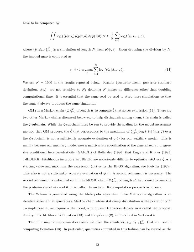
We use N = 1000 in the results reported below. Results (posterior mean, posterior standard

deviation, etc.) are not sensitive to N ; doubling N makes no difference other than doubling

computational time. It is essential that the same seed be used to start these simulations so that

the same θ always produces the same simulation.

GM run a Markov chain ζtKt=1 of length K to compute ζ that solves expression (14). There are

two other Markov chains discussed below so, to help distinguish among them, this chain is called

the ζ-subchain. While the ζ-subchain must be run to provide the scaling for the model assessment

method that GM propose, the ζ that corresponds to the maximum of∑N

t=1 log f(yt | xt−1, ζ) over

the ζ-subchain is not a sufficiently accurate evaluation of g(θ) for our auxiliary model. This is

mainly because our auxiliary model uses a multivariate specification of the generalized autoregres-

sive conditional heteroscedasticity (GARCH) of Bollerslev (1986) that Engle and Kroner (1995)

call BEKK. Likelihoods incorporating BEKK are notoriously difficult to optimize. AG use ζ as a

starting value and maximize the expression (14) using the BFGS algorithm, see Fletcher (1987).

This also is not a sufficiently accurate evaluation of g(θ). A second refinement is necessary. The

second refinement is embedded within the MCMC chain θtRt−1 of length R that is used to compute

the posterior distribution of θ. It is called the θ-chain. Its computation proceeds as follows.

The θ-chain is generated using the Metropolis algorithm. The Metropolis algorithm is an

iterative scheme that generates a Markov chain whose stationary distribution is the posterior of θ.

To implement it, we require a likelihood, a prior, and transition density in θ called the proposal

density. The likelihood is Equation (13) and the prior, π(θ), is described in Section 4.4.

The prior may require quantities computed from the simulation yt, xt−1Nt−1 that are used in

computing Equation (13). In particular, quantities computed in this fashion can be viewed as the

12

evaluation of a functional of the structural model of the form p(·|·, θ) 7→ %, where % ∈ P. Thus,

the prior is a function of the form π(θ, %). But since the functional % is a composite function with

θ 7→ p(·|·, θ) 7→ %, π(θ, %) is essentially a function of θ alone. Thus, we only use π(θ, %) notation

when attention to the subsidiary computation p(·|·, θ) 7→ % is required.

Let q denote the proposal density. For a given θ, q(θ, θ∗) defines a distribution of potential

new values θ∗. We use a move-one-at-a-time, random-walk, proposal density that puts its mass

on discrete, separated points, proportional to a normal. Two aspects of the proposal scheme are

worth noting. The first is that the wider the separation between the points in the support of q

the less accurately g(θ) needs to be computed for α at step 5 of the algorithm below to be correct.

A practical constraint is that the separation cannot be much more than a standard deviation of

the proposal density or the chain will eventually stick at some value of θ. Our separations are

typically 1/2 of a standard deviation of the proposal density. In turn, the standard deviations of

the proposal density are typically no more than the standard deviations in Table 2 and no less

than one order of magnitude smaller. The second aspect worth noting is that the prior is putting

mass on these discrete points in proportion to π(θ). Because we never need to normalize π(θ) this

does not matter. Similarly for the joint distribution f(y|x, g(θ))π(θ) considered as a function of θ.

However, f(y|x, ζ) must be normalized such that∫f(y|x, ζ) dy = 1 to ensure that the implied map

expressed in (14) is computed correctly.

The algorithm for the θ-chain is as follows. Given a current θo and the corresponding ζo = g(θo),

obtain the next pair (θ ′, ζ ′) as follows:

1. Draw θ∗ according to q(θo, θ∗).

2. Draw yt, xt−1Nt=1 according to p(yt|xt−1, θ∗).

3. Compute ζ∗ = g(θ∗) and the functional %∗ from the simulation yt, xt−1Nt=1.

4. Compute α = min(

1, L(θ∗)π(θ∗,%∗) q(θ∗, θo)L(θo)π(θo,%o) q(θo,θ∗)

).

5. With probability α, set (θ ′, ζ ′) = (θ∗, ζ∗), otherwise set (θ′, ζ ′) = (θo, ζo).

It is at step 3 that AG made an important modification to the algorithm proposed by GM. At

that point one has putative pairs (θ∗, ζ∗) and (θo, ζo) and corresponding simulations y∗t , x∗t−1Nt=1

and yot , xot−1Nt=1. AG use ζ∗ as a start and recompute ζo using the BFGS algorithm, obtaining ζo.

13

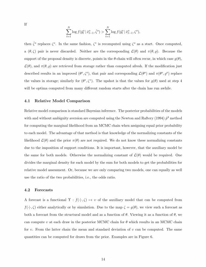
IfN∑t=1

log f(yot | xot−1, ζo) >

N∑t=1

log f(yot | xot−1, ζo),

then ζo replaces ζo. In the same fashion, ζ∗ is recomputed using ζo as a start. Once computed,

a (θ, ζ) pair is never discarded. Neither are the corresponding L(θ) and π(θ, %). Because the

support of the proposal density is discrete, points in the θ-chain will often recur, in which case g(θ),

L(θ), and π(θ, %) are retrieved from storage rather than computed afresh. If the modification just

described results in an improved (θo, ζo), that pair and corresponding L(θo) and π(θo, %o) replace

the values in storage; similarly for (θ∗, ζ∗). The upshot is that the values for g(θ) used at step 4

will be optima computed from many different random starts after the chain has run awhile.

4.1 Relative Model Comparison

Relative model comparison is standard Bayesian inference. The posterior probabilities of the models

with and without ambiguity aversion are computed using the Newton and Raftery (1994) p4 method

for computing the marginal likelihood from an MCMC chain when assigning equal prior probability

to each model. The advantage of that method is that knowledge of the normalizing constants of the

likelihood L(θ) and the prior π(θ) are not required. We do not know these normalizing constants

due to the imposition of support conditions. It is important, however, that the auxiliary model be

the same for both models. Otherwise the normalizing constant of L(θ) would be required. One

divides the marginal density for each model by the sum for both models to get the probabilities for

relative model assessment. Or, because we are only comparing two models, one can equally as well

use the ratio of the two probabilities, i.e., the odds ratio.

4.2 Forecasts

A forecast is a functional Υ : f(·|·, ζ) 7→ υ of the auxiliary model that can be computed from

f(·|·, ζ) either analytically or by simulation. Due to the map ζ = g(θ), we view such a forecast as

both a forecast from the structural model and as a function of θ. Viewing it as a function of θ, we

can compute υ at each draw in the posterior MCMC chain for θ which results in an MCMC chain

for υ. From the latter chain the mean and standard deviation of υ can be computed. The same

quantities can be computed for draws from the prior. Examples are in Figure 6.

14

4.3 The Auxiliary Model

The observed data are yt for t = 1, . . . , n, where yt is a vector of dimension three in our application.

We use the notation xt−1 = yt−1, · · · , yt−L, if the auxiliary model is Markovian, and xt−1 =

yt−1, · · · , y1 if it is not.5 Either way, xt−1 serves as a shorthand for lagged values of yt vector.

In this application, the auxiliary model is not Markovian due to the recursion in expression (17).

The data are modeled as

yt = µxt−1 +Rxt−1zt

where

µxt−1 = b0 +Byt−1, (15)

which is the location function of a one-lag vector auto-regressive (VAR) specification, and Rxt−1 is

the Cholesky factor of

Σxt−1 = R0R′0 (16)

+QΣxt−2Q′ (17)

+P (yt−1 − µxt−2)(yt−1 − µxt−2)′P ′ (18)

+ max[0, V (yt−1 − µxt−2)] max[0, V (yt−1 − µxt−2)]′. (19)

In computations, max(0, x) in expression (19), which is applied element-wise, is replaced by a twice

differentiable cubic spline approximation that plots slightly above max(0, x) over (0.00,0.10) and

coincides elsewhere.

The density h(z) of the i.i.d. zt is the square of a Hermite polynomial times a normal density,

the idea being that the class of such h is dense in Hellenger norm and can therefore approximate a

density to within arbitrary accuracy in Kullback-Leibler distance, see Gallant and Nychka (1987).

Such approximations are often called sieves; Gallant and Nychka term this particular sieve semi-

nonparametric maximum likelihood estimator, or SNP. The density h(z) is the normal when the

degree of the Hermite polynomial is zero. In addition, the constant term of the Hermite polynomial

can be a linear function of xt−1. This has the effect of adding a nonlinear term to the location

function (15) and the variance function (16). It also causes the higher moments of h(z) to depend

5 Refer to Gallant and Long (1997) for the properties of estimators of the form used in this section when the model isnot Markovian.

15

on xt−1 as well. The SNP auxiliary model is determined statistically by adding terms as indicated

by the Bayesian information criteria (BIC) protocol for selecting the terms that comprise a sieve,

see Schwarz (1978).

In our specification, R0 is an upper triangular matrix, P and V are diagonal matrices, and Q

is scalar. The degree of the SNP h(z) density is four. The constant term of the SNP density does

not depend on the past.

The auxiliary model chosen for our analysis, based on BIC, has 1 lag in the conditional mean

component, 1 lag in each of autoregressive conditional heteroscedasticity (ARCH) and generalized

autoregressive conditional heteroscedasticity (GARCH) terms. The model admits leverage effect in

the ARCH term. The auxiliary model has 37 estimated parameters.

The implied error distributions in GSM estimation can differ significantly from the error shocks

used for solving the structural model. For example, we numerically solve the two structural models

in Sections 3 assuming normal distributions for error terms in Equations (1) and (2). This is a

simplifying assumption to ease numerical solutions. The error distributions of simulations from

these models are non-Gaussian. For example, in addition to GARCH and leverage effects, the

three-dimensional error distribution implied by the benchmark smooth ambiguity aversion model

is skewed in all three components and has fat-tails for consumption growth and stock returns and

thin tails for bond returns.

The auxiliary model is determined from simulations of the structural model so issues of data

sparsity do not arise; one can make the simulation length N as large as necessary to determine the

parameters of the auxiliary model accurately. As stated above, we used N = 1,000 and found that

using larger values of N did not change results other than increase run times.

4.4 The Prior and Its Support

Both the benchmark and alternative models are richly parameterized. The benchmark model has

11 structural parameters, given by

θ = (β, γ, ψ, η, p11, p22, κ1, κ2, λ, σc, σd).

The alternative model has 10 parameters with γ = η. The prior is the combination of the product of

independent normal density functions and support conditions. The product of independent normal

16

density functions is given by

π (θ) =

n∏i=1

N[θi|(θ∗i , σ

2θ

)]where n denotes the number of parameters.

For annual data, the prior location parameters of the benchmark model are

θ∗ = (0.9750, 2.00, 1.50, 8.8640, 0.9780, 0.5160,−0.06785, 0.02251, 2.7400, 0.03127, 0.1200).

These values are selected based on Ju and Miao (2012)’s calibration results. With these parameter

values, the calibrated model can roughly reproduce the means and volatilities of the risk-free rate

and stock returns observed in the U.S. data. The scale parameters, i.e., standard deviations, are

σθi = (0.90/1.96)θ∗i . The implication of this choice of standard deviation is that the prior probability

satisfies P (|θi − θ∗i |/|θ∗i | < 0.90) = 0.95, i.e., the probability of θi being within 90 percent of θ∗i

is 0.95. This is a loose prior so that the major determinant of the prior are support conditions

described next. Imposition of a loose prior and mild support conditions provides room for the

equilibrium model to contribute to the identification of estimated parameters. Due to the support

conditions, the effective prior is not an independence prior. For some values of θ∗ proposed in

Step 1 of the θ-chain described in Section 4, a model solution at Step 2 will not exist. In such cases,

α at Step 5 is set to zero.

We constrain the subjective discount factor β to be between 0.00 and 1.00. We bound the

coefficient of risk aversion γ to be above 0.00 and below 15.00, in line with the recommendation of

Mehra and Prescott (1985) that risk aversion should be moderate. Fully parameterized Kreps and

Porteus (1978) and Epstein and Zin (1989) preferences imply a separation between risk aversion

and the IES; therefore we impose γ 6= 1/ψ.6 Following the long-run risk literature (e.g., Bansal

and Yaron (2004)), we impose ψ > 1.00 such that persistent movements in expected consumption

growth are significantly priced in equity returns. The upper bound for ψ is set as ψ < 5.00.

Relaxing this bound has little impact on our estimation results.

We bound η between 2.00 and 100.00. We impose η > γ in the estimation of the benchmark

model. Hayashi and Miao (2011) and Ju and Miao (2012) furnish detailed discussions of this

requirement. Briefly, with η = γ, compound predictive probability distributions are reduced to an

ordinary predictive probability distribution, removing ambiguity from the model. When estimating

6 If γ = 1/ψ, Kreps-Porteus and Epstein-Zin preferences collapse to power utility.

17

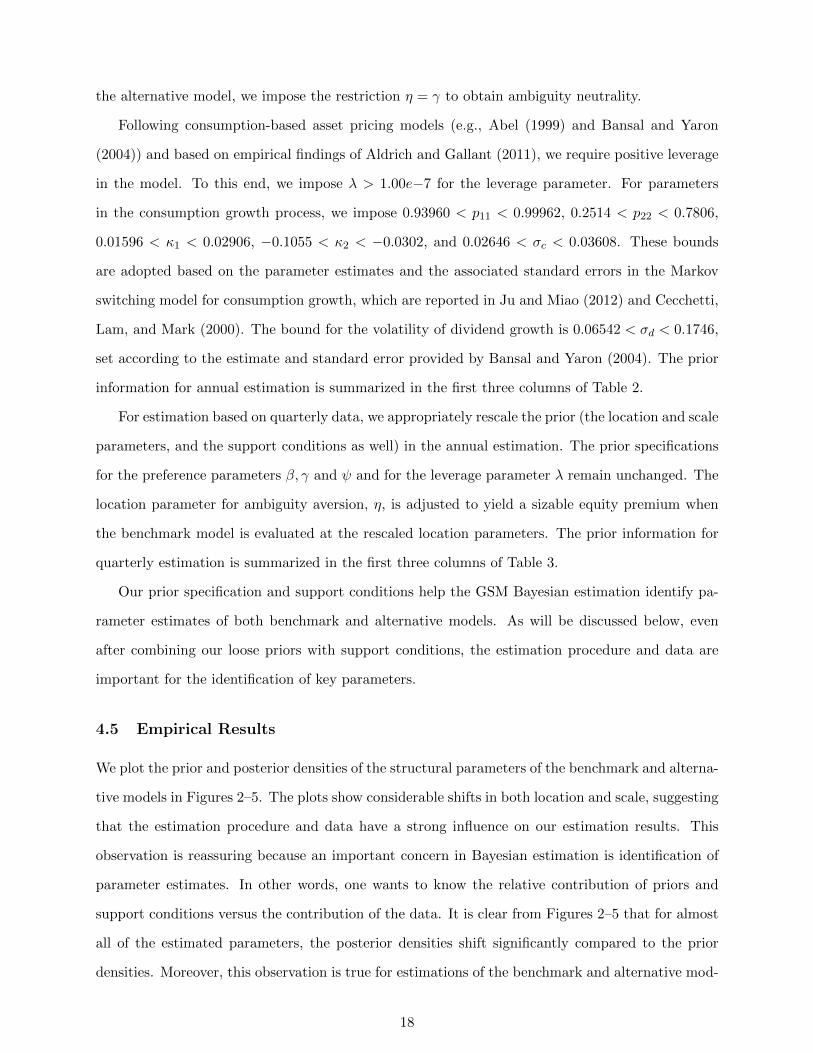
the alternative model, we impose the restriction η = γ to obtain ambiguity neutrality.

Following consumption-based asset pricing models (e.g., Abel (1999) and Bansal and Yaron

(2004)) and based on empirical findings of Aldrich and Gallant (2011), we require positive leverage

in the model. To this end, we impose λ > 1.00e−7 for the leverage parameter. For parameters

in the consumption growth process, we impose 0.93960 < p11 < 0.99962, 0.2514 < p22 < 0.7806,

0.01596 < κ1 < 0.02906, −0.1055 < κ2 < −0.0302, and 0.02646 < σc < 0.03608. These bounds

are adopted based on the parameter estimates and the associated standard errors in the Markov

switching model for consumption growth, which are reported in Ju and Miao (2012) and Cecchetti,

Lam, and Mark (2000). The bound for the volatility of dividend growth is 0.06542 < σd < 0.1746,

set according to the estimate and standard error provided by Bansal and Yaron (2004). The prior

information for annual estimation is summarized in the first three columns of Table 2.

For estimation based on quarterly data, we appropriately rescale the prior (the location and scale

parameters, and the support conditions as well) in the annual estimation. The prior specifications

for the preference parameters β, γ and ψ and for the leverage parameter λ remain unchanged. The

location parameter for ambiguity aversion, η, is adjusted to yield a sizable equity premium when

the benchmark model is evaluated at the rescaled location parameters. The prior information for

quarterly estimation is summarized in the first three columns of Table 3.

Our prior specification and support conditions help the GSM Bayesian estimation identify pa-

rameter estimates of both benchmark and alternative models. As will be discussed below, even

after combining our loose priors with support conditions, the estimation procedure and data are

important for the identification of key parameters.

4.5 Empirical Results

We plot the prior and posterior densities of the structural parameters of the benchmark and alterna-

tive models in Figures 2–5. The plots show considerable shifts in both location and scale, suggesting

that the estimation procedure and data have a strong influence on our estimation results. This

observation is reassuring because an important concern in Bayesian estimation is identification of

parameter estimates. In other words, one wants to know the relative contribution of priors and

support conditions versus the contribution of the data. It is clear from Figures 2–5 that for almost

all of the estimated parameters, the posterior densities shift significantly compared to the prior

densities. Moreover, this observation is true for estimations of the benchmark and alternative mod-

18

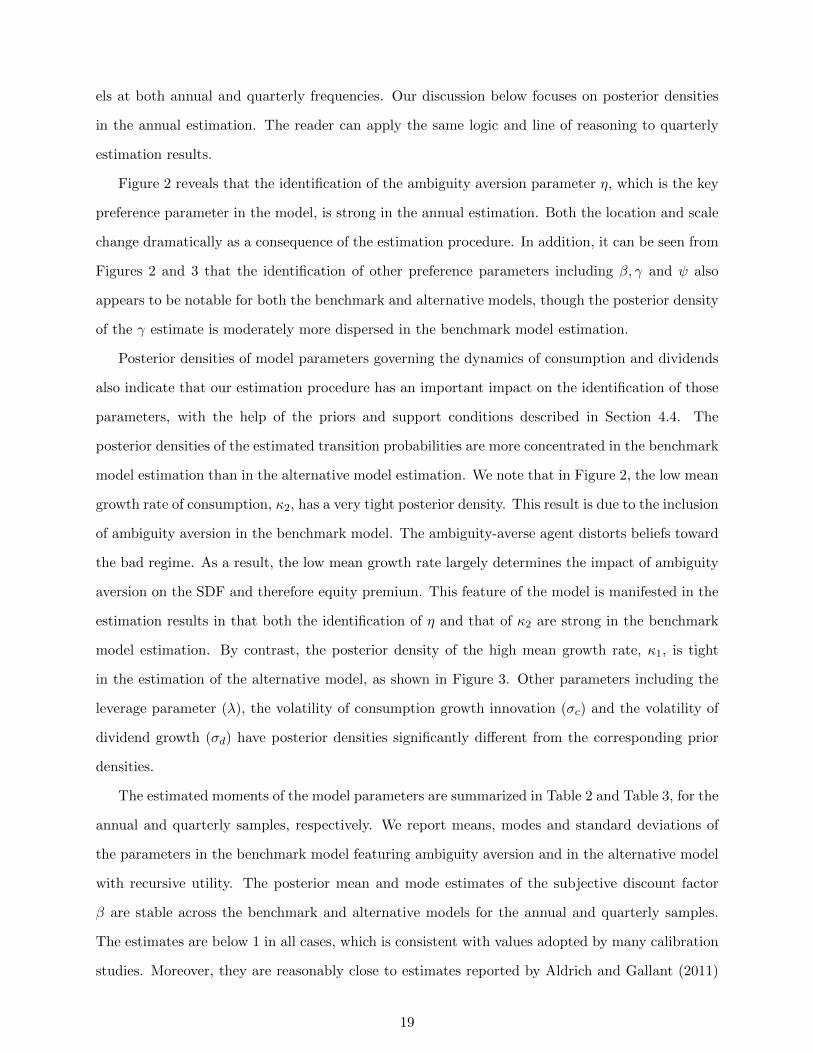
els at both annual and quarterly frequencies. Our discussion below focuses on posterior densities

in the annual estimation. The reader can apply the same logic and line of reasoning to quarterly

estimation results.

Figure 2 reveals that the identification of the ambiguity aversion parameter η, which is the key

preference parameter in the model, is strong in the annual estimation. Both the location and scale

change dramatically as a consequence of the estimation procedure. In addition, it can be seen from

Figures 2 and 3 that the identification of other preference parameters including β, γ and ψ also

appears to be notable for both the benchmark and alternative models, though the posterior density

of the γ estimate is moderately more dispersed in the benchmark model estimation.

Posterior densities of model parameters governing the dynamics of consumption and dividends

also indicate that our estimation procedure has an important impact on the identification of those

parameters, with the help of the priors and support conditions described in Section 4.4. The

posterior densities of the estimated transition probabilities are more concentrated in the benchmark

model estimation than in the alternative model estimation. We note that in Figure 2, the low mean

growth rate of consumption, κ2, has a very tight posterior density. This result is due to the inclusion

of ambiguity aversion in the benchmark model. The ambiguity-averse agent distorts beliefs toward

the bad regime. As a result, the low mean growth rate largely determines the impact of ambiguity

aversion on the SDF and therefore equity premium. This feature of the model is manifested in the

estimation results in that both the identification of η and that of κ2 are strong in the benchmark

model estimation. By contrast, the posterior density of the high mean growth rate, κ1, is tight

in the estimation of the alternative model, as shown in Figure 3. Other parameters including the

leverage parameter (λ), the volatility of consumption growth innovation (σc) and the volatility of

dividend growth (σd) have posterior densities significantly different from the corresponding prior

densities.

The estimated moments of the model parameters are summarized in Table 2 and Table 3, for the

annual and quarterly samples, respectively. We report means, modes and standard deviations of

the parameters in the benchmark model featuring ambiguity aversion and in the alternative model

with recursive utility. The posterior mean and mode estimates of the subjective discount factor

β are stable across the benchmark and alternative models for the annual and quarterly samples.

The estimates are below 1 in all cases, which is consistent with values adopted by many calibration

studies. Moreover, they are reasonably close to estimates reported by Aldrich and Gallant (2011)

19

and Bansal et al. (2007) and also to the GMM estimate of Yogo (2006). Thus, they do not cause

any concern for us and imply precise estimation of the target parameter.

In contrast to the discount factor parameter, estimates of the risk aversion parameter, γ, are

sensitive to the presence of ambiguity aversion. For the annual estimation, the posterior mean

and mode of γ in the alternative model are significantly larger than the corresponding estimates

in the benchmark model. For instance, the posterior mean of γ is 1.62 in the benchmark model,

as opposed to 6.32 in the alternative model. When quarterly data are used for estimation, the

posterior mean and mode of γ in alternative model are an order of magnitude larger than those for

the benchmark model. This result is plausible given the calibration studies of Ju and Miao (2012)

and Collard, Mukerji, Sheppard, and Tallon (2015), who show that with smooth ambiguity aversion,

low risk aversion is required to account for high and time varying equity premium. The result is

also related to the findings of Jeong et al. (2015) for their estimation of the recursive utility model

and the multiple priors model, where aggregate wealth consists of financial wealth only. Jeong et al.

(2015) report estimates of γ ranging between 0.20 to 2.90 in the multiple priors model, while the γ

estimate is 4.90 in the recursive utility model. In comparison with Aldrich and Gallant (2011), the

estimates of γ in the benchmark model with ambiguity aversion are smaller than their estimates for

both habit formation and long-run risk models, but similar to their prospect theory-based results.

The posterior mode and mean of the ambiguity aversion parameter η are 29.80 and 30.33 for

the annual sample and 57.08 and 55.93 for the quarterly sample.7 The standard deviation of the

posterior distribution of η is consistently low. Taken together, tightly estimated values for η and the

impact of modeling ambiguity aversion on estimation of risk aversion parameter, γ, strongly imply

that ambiguity aversion does explain important features of asset returns in the data, namely low

risk-free rates, high equity premium and volatile equity returns. Since all of the model parameters

are estimated simultaneously by the GSM Bayesian estimation methodology, the posterior estimates

of the ambiguity aversion parameter depend on the estimation results for other model parameters

especially primitive parameters in the consumption growth process. Using the post-war data, our

quarterly estimation generates parameter estimates in the consumption growth process that are

quite different from the results in the annual estimation. This observation explains the difference

between annual and quarterly estimates of the ambiguity aversion parameter. Typical values used

7 Thimme and Volkert (2015) use quarterly data to estimate the ambiguity aversion parameter in the smooth ambiguityutility function adopted in our study. Their GMM estimation relies on fixed values for the IES parameter anda reduced-form, linearized SDF. They obtain estimates of η ranging from 24 to 62, which are comparable to ourstructural estimation results.

20

in the calibration studies, for example, η = 8.86 in Ju and Miao (2012) and η = 19 in Jahan-Parvar

and Liu (2014), provide a lower bound for our estimates.8

Ahn et al. (2014) conduct an experimental study on estimating smooth ambiguity aversion.

Based on a static formulation, they report values of an ambiguity aversion parameter ranging

between 0.00 and 2.00, with a mean value of 0.207. Their estimates of the ambiguity aversion

parameter are statistically insignificant and are at least an order of magnitude smaller than our

dynamic model-based estimates. We believe that ignoring intertemporal choice under ambiguity

explains these differences in estimates of ambiguity aversion.9

There is an ongoing debate about the value of the IES parameter ψ in the asset pricing literature.

This parameter is crucial for equilibrium asset pricing models to match macroeconomic and financial

moments in the data. In the empirical literature, some studies (e.g., Hall (1988) and Ludvigson

(1999)) find that the IES estimates are close to zero as implied by aggregate consumption data.

Other studies find higher values using cohort- or household-level data (e.g., Attanasio and Weber

(1993) and Vissing-Jorgensen (2002)). Attanasio and Vissing-Jorgensen (2003) find that the IES

estimate for stockholders is typically above 1. Bansal and Yaron (2004) point out that the IES

estimates will be under-estimated unless heteroscedasticity in aggregate consumption growth and

asset returns is taken into account.

Our estimation strongly suggests an IES greater than unity, as advocated by the long-run risk

literature. Tables 2 and 3 present the posterior mode and mean of the IES parameter, ψ, estimated

in the annual and quarterly samples respectively. The posterior mode and mean estimates range

from 2.50 to 5.00 across different models with small standard deviations. These estimates are

larger than those reported by Aldrich and Gallant (2011), which are in the neighborhood of 1.50.

Risk aversion and the IES both determine the representative agent’s preference for the timing of

resolution of uncertainty. If γ > 1/ψ, the agent prefers earlier resolution of uncertainty; see Epstein

and Zin (1989) and Bansal and Yaron (2004). Given the high estimates of ψ, both benchmark and

alternative models point to a representative agent who prefers an earlier resolution of uncertainty.

Adding ambiguity aversion attenuates this preference moderately: Once ambiguity aversion is taken

8 Ju and Miao (2012) calibrate their consumption-based model to a century-long data sample starting from late 19thcentury. Jahan-Parvar and Liu (2014) calibrate their model to match features of data on both the business cycle andasset returns based on 19230–2010 data.

9 We find that the difference in the magnitude of these estimates is similar to the difference between static estimatesof Gul (1991) disappointment aversion parameter reported by Choi, Fisman, Gale, and Kariv (2007) and dynamicestimates reported by Feunou, Jahan-Parvar, and Tedongap (2013). Thus, the difference is more likely to be anoutcome of the static setting used rather than using different estimation methods, such as GSM Bayesian methodologyin our case and a frequentist method in case of Feunou et al.

21

into account, the estimates of ψ are around 2.62 – 2.96 in annual estimates and 4.28 – 4.55 for

quarterly data. The GSM estimation delivers stable estimates of the IES parameter. This is in

contrast to the results of Jeong et al. (2015), where the ψ estimates range from 0.00 to ∞. In

particular, when only financial wealth is used to proxy total wealth and ambiguity is represented

by multiple priors, Jeong et al. (2015) obtain estimates of ψ that are equal to 0.68 with time-varying

volatility and 11.16 with nonlinear stochastic volatility.

Table 2 and Table 3 present posterior mean and mode estimates of the primitive parameters

in the consumption growth process for the annual and quarterly estimations respectively. The

results indicate that the GSM estimation method can successfully identify two distinct regimes of

consumption growth for both benchmark and alternative models. The difference between κ1 and κ2

estimates is sizable. The transition probability estimate of p11 is above 0.90 in all cases, while the

estimate of p22 is about 0.30 – 0.40 in the annual estimation and about 0.70 – 0.80 in the quarterly

estimation. This result suggests that the good regime is very persistent while the bad regime is

transitory. All these estimates together with the estimates for volatility of the growth innovation,

σc, have low standard deviations. Compared with empirical estimates reported by Cecchetti, Lam,

and Mark (2000), differences in several parameter estimates are noticeable. However, this is not

surprising. Cecchetti, Lam, and Mark (2000) fit a Markov switching model to consumption data

only. Our GSM estimation uses both consumption data and asset returns data to estimate the

model. Besides, we use different sample periods.

Dividend growth, ∆dt, is a latent variable in our estimation. In the benchmark annual esti-

mation, the posterior estimates of the leverage parameter λ are moderately greater than 1. This

is consistent with the argument of Abel (1999) that aggregate dividends are a levered claim on

aggregate consumption. However, the estimates of λ are lower than the value used in the calibra-

tion of Ju and Miao (2012) where λ = 2.74. In the alternative model estimation at the annual

frequency, estimates of λ shown on Table 2 are closer to this value. In the quarterly estimation,

the posterior mean estimates of λ are between 1 and 2. The volatility estimate of dividend growth

is stable across different models and samples. Our estimates of λ and σd are not directly compara-

ble to results of Aldrich and Gallant (2011) or Bansal et al. (2007) due to different specifications

for modeling dividend growth. Specifically, Aldrich and Gallant (2011) and Bansal et al. (2007)

estimate the long-run risk model featuring time variation in the volatility of fundamentals, while

we rely on Markov-switching mean growth rates and learning to generate time-varying volatility

22

of equity returns. However, our estimates of σd are close in magnitude to that in the estimated

prospect theory model reported by Aldrich and Gallant (2011). Aldrich and Gallant posit constant

volatility for the dividend growth process in the prospect theory model.

In summary, apart from estimates for the risk aversion parameter and ambiguity aversion param-

eter, estimates of other structural parameters in our study are remarkably stable and are generally

comparable in magnitude to values reported by other empirical asset pricing studies. Thus, it is

reasonable to believe that parameter estimates other than risk aversion and ambiguity aversion

estimates have small influence on identification and model comparison when it comes to the model

featuring smooth ambiguity aversion. In addition, ignoring ambiguity aversion can lead to biased

estimates of the risk aversion parameter.

5 Model Comparison and Implications

5.1 Relative Model Comparison

Relative model comparison is standard Bayesian inference as described in Subsection 4.1. The

computed odds ratio is 1/6.09e− 85 for the annual estimation and 1/1.18e− 36 for the quarterly

estimation, which strongly favors the benchmark model over the alternative model. This ratio

implies that our benchmark model provides a better description of the available data. Given the

logarithmic values of posterior evaluated at the mode for the benchmark and alternative models

reported in Tables 2 and 3, it is also obvious that the benchmark model is the preferred model. One

can gain a rough appreciation for what these odds ratios indicate from a frequentist perspective by

disregarding the effects of the prior and support conditions and comparing the log posteriors shown

in Tables 2 and 3 as if they were log likelihoods. For the annual comparison minus twice the log

likelihood ratio gives a χ2-statistic equal to 260.00 on one degree of freedom and for the quarterly

data 82.70 on one degree of freedom. The p-value for either is less than 0.0001.

5.2 Forecasts

Forecasts are constructed as described in Subsection 4.2. Prior forecasts (not shown) do not differ

much between pre- and post-Great Recession periods. There are, however, differences between

prior forecasts based on the benchmark model and the alternative model. The main difference is

the disparity in the level of benchmark and alternative model-based forecasts of the short rate. The

23

benchmark model forecasts a higher level for the short rate and a wider standard deviations than

the alternative model does. The second difference is the slight increase in the consumption growth

path forecasted by the benchmark model, against the drop forecasted by the alternative model.

Prior forecasts are not a measure of a model’s success in predicting the data dynamics. For

that purpose, we rely on posterior forecasts shown in Figure 6.10 As Figure 6 shows, the posterior

forecasts of consumption growth differ across the pre- and post-Great Recession episodes. Both

benchmark and alternative models forecast a drop in consumption growth for the pre-recession

period while a slight increase for the post-recession period based on available information by the end

of 2011. The posterior forecasts paths generated by both modes are on average similar. However,

the benchmark model implies slightly more variation in consumption growth forecasts.

For the pre-recession period, the benchmark model forecasts a steeper drop in stock returns

compared to the alternative model. For the post-recession period, the benchmark model yields

posterior return forecasts that are lower than those generated by the alternative model. These

results reflect the pessimism inherent in our benchmark model with ambiguity aversion. Based on

data up to the Great Recession period, Aldrich and Gallant (2011) report posterior forecasts of

stock returns generated from the long-run risk model. Their return forecasts are roughly 6% for

the period 2009–2013. Given the recent past experience, this level appears to be high.

It is clear from Figure 6 that the benchmark model predicts overall lower short rates compared to

the alternative model’s forecasts. Moreover, the benchmark model predicts a drop in the short rate

for both pre- and post-recession periods while the alternative model implies the opposite results.11

These results about the posterior forecasts echo the mechanism of earlier models on ambiguity

(or uncertainty) that the induced higher precautionary savings motive tends to reduce the risk-free

rate. Given recent announcements by various practitioners, academicians and former policy makers

about the likelihood of interest rates reverting back to “old normal” levels, the posterior forecasts

generated by our benchmark model seem reasonable.12

Given that Bayesian model comparison prefers the benchmark model over the alternative model,

10 We find a rather dramatic change in the standard errors between the prior and posterior forecasts. This resultsuggests that the data is quite informative for the forecasts. The impact can also be confirmed by comparing theprior and posterior estimates of model parameters reported in Tables 2 and 3 and the prior and posterior densitiesof the estimated parameters shown in Figures 2 to 5.

11 While this observation is in line with the zero-lower bound environment since the Great Recession, they should not beviewed as synonymous. We are forecasting real risk-free rates. They are not influenced by fiscal or monetary policyand are endogenously determined in the model.

12 For example, on May 16, 2014 the former Federal Reserve Chairman Ben Bernanke opined that low interest rateenvironment is likely to continue beyond many then-current forecasts. (Source: Reuters)

24

our results of posterior forecasts merit attention. The two models lead to very different dynamics

for consumption growth and asset returns. If we indeed live in a world populated by ambiguity-

averse agents, then policy and decision makers need to be aware of the inherently different attitudes

and hence, market behavior of agents endowed with ambiguity aversion preferences, as opposed to

those assumed in standard rational expectation models.

5.3 Asset Pricing Implications

In this section, we study the asset pricing implications of the benchmark model, using the esti-

mated model parameters. Unlike calibration studies, our focus here is not to match unconditional

moments of asset returns in the data as closely as possible. Instead, we want to assess the impact

of ambiguity aversion on equity premium and the price of risk based on our estimated model rather

than independently chosen parameter values. If the estimated benchmark model is reasonably suc-

cessful in reproducing high price of risk and unconditional equity premium that are not explicitly

targeted in our estimation, we view this outcome as confirmation that the dynamics of asset prices

implied by our estimation are reasonably close to the underlying data generating process (DGP).

Table 4 presents key financial moments generated by both benchmark and alternative models

when model parameters are set to their posterior mean values reported in Table 2.13 Although

matching financial moments is not set an explicit target in our estimation, the estimated benchmark

model implies moments of asset returns close to the data. All moments reported in 4 are annualized.

We observe the following. First, under the benchmark model, the risk-free rate has a mean of about

1 percent and low volatility. Low volatility of the risk-free rate is due to the high estimate of the IES

parameter, which implies strong intertemporal substitution effect, see Bansal and Yaron (2004).

The mean risk-free rate implied by the alternative model is 1.44 percent and is much higher than

the data, at 1.07 percent.

Second, while both benchmark and alternative models generate volatility of equity returns

close to the data, the two models differ dramatically in terms of their performance in producing

high equity premium. The mean equity premium implied by the benchmark model estimation

is 7.31 percent, close to that in the annual sample at 7.47 percent. In contrast, the alternative

model implies a mean equity premium of 1.36 percent. As shown by Bansal and Yaron (2004),

13 The benchmark model estimated using the quarterly sample can also produce high price of risk and equity premium.For the sake of brevity, the unconditional financial moments are not reported for this case. Results are available uponrequest from the authors.

25

without high risk aversion or time-varying uncertainty, the long-run risk model with Epstein and

Zin preferences has difficulty in matching the mean equity premium. For that reason, Bansal and

Yaron consider long-run risk in the mean of consumption growth and also set γ = 10 to match the

mean equity premium. Since the estimated γ for the alternative model is smaller (E(γ) = 6.32 and

σ(γ) = 0.26) and the model abstracts from stochastic volatility, the mean equity premium implied

by the alternative model is too low.

Third, the market price of risk, defined by σ(M)/E(M), is closely related to moments of equity

returns via the Hansen-Jagannathan bound

∣∣∣∣∣∣E(Ret −R

ft

)σ(Ret −R

ft

)∣∣∣∣∣∣ ≤ σ (Mt)

E (Mt).

A reasonable model that can explain asset prices data well should deliver a SDF that satisfies the

bound. The price of risk under the alternative model is 0.28, whereas the Sharpe ratio is 0.37 in the

annual sample. It is obvious that the estimated alternative model violates the Hansen-Jagannathan

bound. The estimated benchmark model generates σ (Mt) /E (Mt) = 2.63 and thus satisfies the

bound. In addition, the Sharpe ratio implied by the benchmark model is 0.42, close to the data at

0.37.

Figure 7 plots conditional equity premium, equity volatility, price of risk and the price-dividend

ratio as functions of the state belief µt, the posterior probability of the high mean regime of

consumption growth. The results are similar to conditional moments plotted by Ju and Miao

(2012) except that our results are based on estimated model parameters. Under the alternative

model with Epstein and Zin’s preferences, conditional equity premium, equity volatility and price

of risk display humped shapes. The maximum of these conditional moments is attained when µt is

close to 0.50 due to high uncertainty induced by Bayesian learning. Ambiguity aversion increases

conditional equity premium and price of risk significantly for values of µt near its steady-state

level implied by the estimated Markov-switching model. The intuition is that the agent distorts

her beliefs pessimistically in the face of a shock to consumption growth and thus demands high

risk premium. Because the high mean growth regime is persistent, the distribution of µt is highly

skewed toward 1.00. Thus, the impact of ambiguity aversion on conditional price of risk and

equity premium is strong when µt is close to its steady-state value. The pessimistic distortion also

yields lower price-dividend ratios in the benchmark model, as shown in Panel D, Figure 7. Similar

26

to Ju and Miao (2012), our estimated benchmark model can also reproduce the countercyclical

pattern of equity premium and equity volatility. The simulation results are plotted in Figure 8. We

observe that the distorted belief puts more probability weight on the bad regime. When shocks to

consumption growth are large in magnitude, the distorted belief becomes even more pessimistic and

conditional equity premium and equity volatility rise significantly. Thus, the model can reproduce

volatility clustering, which is also captured by the auxiliary model used in our estimation.

Finally, an important question is: Do our structural estimations imply reasonable magnitudes

for ambiguity aversion? To address this question, we use detection-error probabilities to assess the

room for ambiguity aversion based on our estimation results. This exercise is meaningful because

our estimation is grounded in the data and thus is informative about the behavior of economic

agents and the dynamics of economic variables.

Detection-error probabilities are an approach developed by Anderson, Hansen, and Sargent

(2003) and Hansen and Sargent (2010) to assess the likelihood of making errors in selecting statis-

tically “close” (in terms of relative entropy) data generating processes (DGP). In this study, the

reference DGP refers to the Markov switching model specified in Equation (1). Without ambiguity

aversion, the transition probabilities of the Markov chain are defined by p11 and p22. Ambigu-

ity aversion implies distortion to the transition probabilities and thus gives rise to the distorted

DGP. The Appendix shows that the reference DGP and the distorted DGP differ only in terms

of transition probabilities. We adapt the approach of computing detection-error probabilities in

Jahan-Parvar and Liu (2014) to the endowment economy in our study. This approach enables us

to simulate artificial data from the reference and distorted DGPs and then evaluate the likelihood

explicitly. Details of the algorithm are available in the Appendix.

A sizable detection-error probability (p(η)) associated with a certain value of the ambiguity

aversion parameter, η, implies that there is a large chance of making mistakes in distinguishing the

reference DGP from the distorted DGP, and thus ample room exists for ambiguity aversion. Based

on the estimated parameters of the benchmark model, the detection-error probability is 10.22% for

the annual estimation and 13% for the quarterly estimation. Anderson, Hansen, and Sargent (2003)

advocates that a detection-error probability of about 10% suggests plausible extent for ambiguity.

Thus, our estimated model parameters admit reasonably large scope for ambiguity aversion.

27

6 Conclusion

Smooth ambiguity preferences of Klibanoff et al. (2005, 2009) have gained considerable popularity

in recent years. This popularity is due to clear separation between ambiguity, which is a charac-

teristic of the representative agent’s subjective beliefs, and ambiguity aversion that derives from

the agent’s tastes. In this paper, we estimate the endowment equilibrium asset pricing model with

smooth ambiguity preferences proposed by Ju and Miao (2012) using U.S. data and GSM Bayesian

estimation methodology of Gallant and McCulloch (2009) to: (1) investigate the empirical proper-

ties of such an asset pricing model as an adequate characterization of the returns and consumption

growth data and, (2) provide an empirical estimation of the ambiguity aversion parameter and its

relationship with other structural parameters in the model. Our study contributes to the existing

literature by providing a formal empirical investigation for adequacy of this class of preferences for

economic modeling and presenting estimations for the structural parameters of this model. The

estimated structural parameters are in line with theoretical expectations and are comparable with

estimated parameters in related studies. With respect to measurement of ambiguity aversion, our

results show a marked improvement over the existing literature. The existing empirical literature

either provides measures of ambiguity (which is usually the size of the set of priors in the MPU

framework) instead of ambiguity aversion of the agent, or implausible estimates (economically or

statistically) for smooth ambiguity aversion parameter. Our study addresses both shortcoming in

the extant literature.

We find that Bayesian model comparison strongly favors the benchmark model featuring a rep-

resentative agent endowed with smooth ambiguity preferences, over the alternative model featuring

Epstein-Zin’s recursive preferences. Our estimates of the ambiguity aversion parameter are large

and have important asset pricing implications for the market price of risk and equity premium.

Detection-error probabilities computed using the estimated parameters imply ample scope for am-

biguity aversion. Structural estimations ignoring ambiguity aversion may lead to biased estimates

of the risk aversion parameter and are unable to explain the high market price of risk implied by

financial data. Our estimates of the IES parameter are significantly greater than 1 and suggest

a strong preference for earlier resolution of uncertainty, as is consistent with the long-run risk

literature.

28

References

Abel, A. B., 1999. Risk premia and term premia in general equilibrium. Journal of MonetaryEconomics 43 (1), 3–33.

Ahn, D., Choi, S., Gale, D., Kariv, S., 2014. Estimating ambiguity aversion in a portfolio choiceexperiment. Quantitative Economics 5 (2), 195–223.

Aldrich, E. M., Gallant, A. R., 2011. Habit, long-run risks, prospect? a statistical inquiry. Journalof Financial Econometrics 9, 589–618.

Anderson, E. W., Ghysels, E., Juergens, J. L., 2009. The impact of risk and uncertainty on expectedreturns. Journal of Financial Economics 94, 233–263.

Anderson, E. W., Hansen, L. P., Sargent, T. J., 2003. A quartet of semigroups for model spec-ification, robustness, price of risk, and model detection. Journal of the European EconomicAssociation 1, 68–123.

Andreski, P., Li, G., Samancioglu, M. Z., Schoeni, R., 2014. Estimates of annual consumptionexpenditures and its major components in the PSID in comparison to the CE. American EconomicReview: Papers and Proceedings 104 (5), 132–135.

Attanasio, O. P., Vissing-Jorgensen, A., 2003. Stock-market participation, intertemporal substitu-tion and risk aversion. American Economic Review Papers and Proceedings 93, 383–391.

Attanasio, O. P., Weber, G., 1993. Consumption growth, the interest rate and aggregation. Reviewof Economic Studies 60, 631–649.

Backus, D., Ferriere, A., Zin, S., 2015. Risk and ambiguity in models of business cycles. Journal ofMonetary Economics 69, 42–63.

Bansal, R., Gallant, R., Tauchen, G., 2007. Rational pessimism and exuberance. Review of Eco-nomic Studies 74, 1005–1033.

Bansal, R., Yaron, A., 2004. Risks for the long run: A potential resolution of asset pricing puzzles.Journal of Finance 59, 1481–1509.

Bianchi, F., Ilut, C., Schneider, M., 2014. Uncertainty shocks, asset supply and pricing over thebusiness cycle. Working Paper.

Bollerslev, T., 1986. Generalized autoregressive conditional heteroskedasticity. Journal of Econo-metrics 31, 307–327.

Cecchetti, S. G., Lam, P.-S., Mark, N. C., 2000. Asset pricing with distorted beliefs: Are equityreturns too good to be true? American Economic Review 90, 787–805.

Chen, H., Ju, N., Miao, J., 2014. Dynamic asset allocation with ambiguous return predictability.Review of Economic Dynamics 17, 799–823.

Chen, Z., Epstein, L., 2002. Ambiguity, risk, and asset returns in continuous time. Econometrica70 (4), 1403–1443.

Choi, S., Fisman, R., Gale, D., Kariv, S., 2007. Consistency, heterogeneity, and granularity ofindividual behavior under uncertainty. American Economic Review 97 (5), 1921–1938.

Collard, F., Mukerji, S., Sheppard, K., Tallon, J.-M., 2015. Ambiguity and the historical equitypremium. Working Paper, University of Oxford.

29

Engle, R. F., Kroner, K. F., 1995. Multivariate Simulteneous Generalized ARCH. EconometricTheory 11 (1), 122–150.

Epstein, L. G., Zin, S. E., 1989. Substitution, risk aversion, and the temporal behavior of consump-tion and asset returns: A theoretical framework. Econometrica 57 (4), 937–969.

Feunou, B., Jahan-Parvar, M. R., Tedongap, R., 2013. Modeling market downside volatility. Reviewof Finance 17 (1), 443–481.

Fletcher, R., 1987. Practical Methods of Optimization, 2nd Edition. John Wiley and Sons, NewYork, NY.

Gallant, A. R., Long, J. R., 1997. Estimating stochastic differential equations efficiently by minimumchi-squared. Biometrica 84, 125–141.

Gallant, A. R., McCulloch, R. E., 2009. On the determination of general scientific models withapplication to asset pricing. Journal of the American Statistical Association 104, 117–131.

Gallant, A. R., Nychka, D. W., 1987. Seminonparametric maximum likelihood estimation. Econo-metrica 55, 363–390.

Gallant, A. R., Tauchen, G., 1996. Which moments to match? Econometric Theory 12, 657–681.

Gallant, A. R., Tauchen, G., 1998. Reprojecting partially observed systems with application tointerest rate diffusions. Journal of the American Statistical Association 93, 10–24.

Gallant, A. R., Tauchen, G., 2010. Handbook of Financial Econometrics. Vol. 1 Tools and Tech-niques. Elsevier/North-Holland, Amsterdam, Ch. Simulated Score Methods and Indirect Infer-ence for Continuous-time Models, pp. 427–478.

Gamerman, D., Lopes, H. F., 2006. Markov Chain Monte Carlo: Stochastic Simulation for BayesianInference, 2nd Edition. No. 86 in CRC Texts in Statistical Science. Chapman & Hall, New York,NY.

Garner, T. I., Janini, G., Passero, W., Paszkiewicz, L., Vendemia, M., September 2006. The CEand the PCE: A Comparison. Monthly Labor Review, Bureau of Labor Statistics (09).

Gollier, C., 2011. Portfolio choices and asset prices: The comparative statics of ambiguity aversion.Review of Economic Studies 78, 1329–1344.

Gourieroux, C., Monfort, A., Renault, E. M., 1993. Indirect inference. Journal of Applied Econo-metrics 8, S85–S118.

Guidolin, M., Liu, H., 2014. Ambiguity aversion and under-diversification. Journal of Financial andQuantitative Analysis, forthcoming.

Gul, F., 1991. A theory of disappointment aversion. Econometrica 59 (3), 667–686.

Halevy, Y., 2007. Ellsberg revisited: An experimental study. Econometrica 75, 503–536.

Hall, R., 1988. Intertemporal substitution in consumption. Journal of Political Economy 96, 339–357.

Hansen, L. P., 2007. Beliefs, doubts and learning: The valuation of macroeconomic risk. AmericanEconomic Review 97, 1–30.

30

Hansen, L. P., Sargent, T. J., 2010. Fragile beliefs and the price of uncertainty. QuantitativeEconomics 1, 129–162.

Hayashi, T., Miao, J., 2011. Intertemporal substitution and recursive smooth ambiguity preferences.Theoretical Economics 6.

Ilut, C., Schneider, M., 2014. Ambiguous business cycles. American Economic Review 104, 2368–2399.

Jahan-Parvar, M. R., Liu, H., 2014. Ambiguity aversion and asset prices in production economies.Review of Financial Studies 27 (10), 3060–3097.

Jarque, C. M., Bera, A. K., 1980. Efficient tests for normality, homoscedasticity and serial inde-pendence of regression residuals. Economics Letters 6 (3), 255–259.

Jeong, D., Kim, H., Park, J. Y., 2015. Does ambiguity matter? Estimating asset pricing modelswith a multiple-priors recursive utility. Journal of Financial Economics 115 (2), 361–382.

Ju, N., Miao, J., 2012. Ambiguity, learning, and asset returns. Econometrica 80, 559–591.

Klibanoff, P., Marinacci, M., Mukerji, S., 2005. A smooth model of decision making under ambiguity.Econometrica 73 (6), 1849–1892.

Klibanoff, P., Marinacci, M., Mukerji, S., 2009. Recursive smooth ambiguity preferences. Journalof Economic Theory 144 (3), 930–976.

Kreps, David, M., Porteus, E. L., 1978. Temporal resolution of uncertainty and dynamic choice.Econometrica 46, 185–200.

Ludvigson, S. C., 1999. Consumption and credit: A model of time-varying liquidity constraints.Review of Economics and Statistics 81, 434–447.

Maccheroni, F., Marinacci, M., Ruffino, D., 2013. Alpha as ambiguity: Robust mean-varianceportfolio analysis. Econometrica 81 (3), 1075–1113.

Mehra, R., Prescott, E. C., 1985. The equity premium: a puzzle. Journal of Monetary Economics15, 145–161.

Newton, M. A., Raftery, A. E., 1994. Approximate bayesian inference with the weighted likelihoodbootstrap. Journal of the Royal Statistical Society - Series B 56, 3–48.

Ruffino, D., 2013. A robust capital asset pricing model. Working Paper, Federal Reserve Board.

Schwarz, G., 1978. Estimating the dimension of a model. Annals of Statistics 6, 461–464.

Strzalecki, T., 2013. Temporal resolution of uncertainty and recursive models of ambiguity aversion.Econometrica 81 (3), 1039–1074.

Thimme, J., Volkert, C., 2015. Ambiguity in the cross-section of expected returns: An empiricalassessment. Journal of Business & Economic Statistics, forthcoming 33 (3), 418–429.

Veronesi, P., 1999. Stock market overreaction to bad news in good times: A rational expectationsequilibrium model. Review of Financial Studies 12, 975–1007.

Viale, A. M., Garcia-Feijoo, L., Giannetti, A., 2014. Safety first, learning under ambiguity, and thecross-section of stock returns. Review of Asset Pricing Studies 4 (1), 118–159.

31

Vissing-Jorgensen, A., 2002. Limited asset market participation and the elasticity of intertemporalsubstitution. Journal of Political Economy 110, 825–853.

Yogo, M., 2006. A consumption-based explanation of expected stock returns. Journal of Finance61, 539–580.

32

7 Appendix: Detection-error Probabilities

• In constructing distorted transition probabilities, we consider a “full information model”,where the agent is ambiguity averse but state zt is observable. In this case, the Euler equationis

0 = p11E1,t

[Mzt+1,t+1

(Ret+1 −R

ft

)]+ (1− p11)E2,t

[Mzt+1,t+1

(Ret+1 −R

ft

)]for zt = 1 and

0 = (1− p22)E1,t

[Mzt+1,t+1 (Re,t+1 −Rf,t)

]+ p22E2,t

[Mzt+1,t+1 (Re,t+1 −Rf,t)

]for zt = 2. The Euler equation can be rewritten as

0 = p11E1,t

[MEZzt+1,t+1

(Ret+1 −R

ft

)]+ (1− p11)E2,t

[MEZzt+1,t+1

(Ret+1 −R

ft

)]0 = (1− p22)E1,t

[MEZzt+1,t+1

(Ret+1 −R

ft

)]+ p22E2,t

[MEZzt+1,t+1

(Ret+1 −R

ft

)]where MEZ

zt+1,t+1 is the SDF under recursive utility without ambiguity aversion, and p11 andp22 are distorted transition probabilities and are given by

p11 =p11

p11 + (1− p11)

E2

[V 1−γzt+1,t+1

]E1

[V 1−γzt+1,t+1

]−

η−γ1−γ

, (20)

p22 =p22

(1− p22)

E1

[V 1−γzt+1,t+1

]E2

[V 1−γzt+1,t+1

]−

η−γ1−γ

+ p22

, (21)

where Vzt,t, (zt = 1, 2) are solutions to the following value function under full information:

Vzt,t(C) =

[(1− β)C

1− 1ψ

t + βRzt

(Vzt+1,t+1 (C)

)1− 1ψ

] 1

1− 1ψ ,

Rzt(Vzt+1,t+1 (C)

)=

(Ezt[(

Ezt+1,t

[V 1−γzt+1,t+1 (C)

]) 1−η1−γ]) 1

1−η

.

• The numerical algorithm of calculating detection-error probabilities takes the following steps:

1. Repeatedly draw ∆ctTt=1 under the reference data generating process (DGP), which isthe two-state Markov switching model with transition probabilities p11 and p22.

2. Evaluate the log likelihood function under the reference DGP by computing

lnLrT =T∑t=1

ln

2∑

zt=1

f (∆ct|zt) Pr (zt|Ωt−1)

where πt−1 = Pr (zt = 1|Ωt−1) are filtered probabilities implied by the Markov switchingmodel.

33

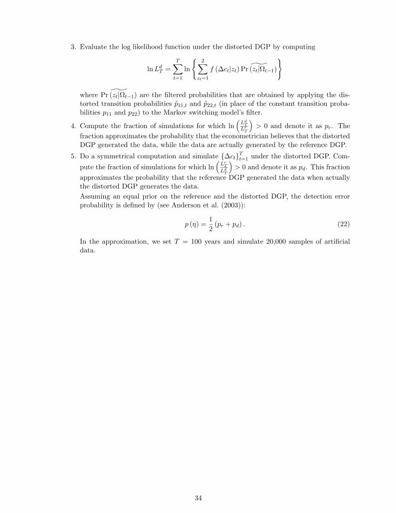
3. Evaluate the log likelihood function under the distorted DGP by computing

lnLdT =T∑t=1

ln

2∑

zt=1

f (∆ct|zt) ˜Pr (zt|Ωt−1)

where ˜Pr (zt|Ωt−1) are the filtered probabilities that are obtained by applying the dis-torted transition probabilities p11,t and p22,t (in place of the constant transition proba-bilities p11 and p22) to the Markov switching model’s filter.

4. Compute the fraction of simulations for which ln(LdTLrT

)> 0 and denote it as pr. The

fraction approximates the probability that the econometrician believes that the distortedDGP generated the data, while the data are actually generated by the reference DGP.

5. Do a symmetrical computation and simulate ∆ctTt=1 under the distorted DGP. Com-

pute the fraction of simulations for which ln(LrTLdT

)> 0 and denote it as pd. This fraction

approximates the probability that the reference DGP generated the data when actuallythe distorted DGP generates the data.

Assuming an equal prior on the reference and the distorted DGP, the detection errorprobability is defined by (see Anderson et al. (2003)):

p (η) =1

2(pr + pd) . (22)

In the approximation, we set T = 100 years and simulate 20,000 samples of artificialdata.

34

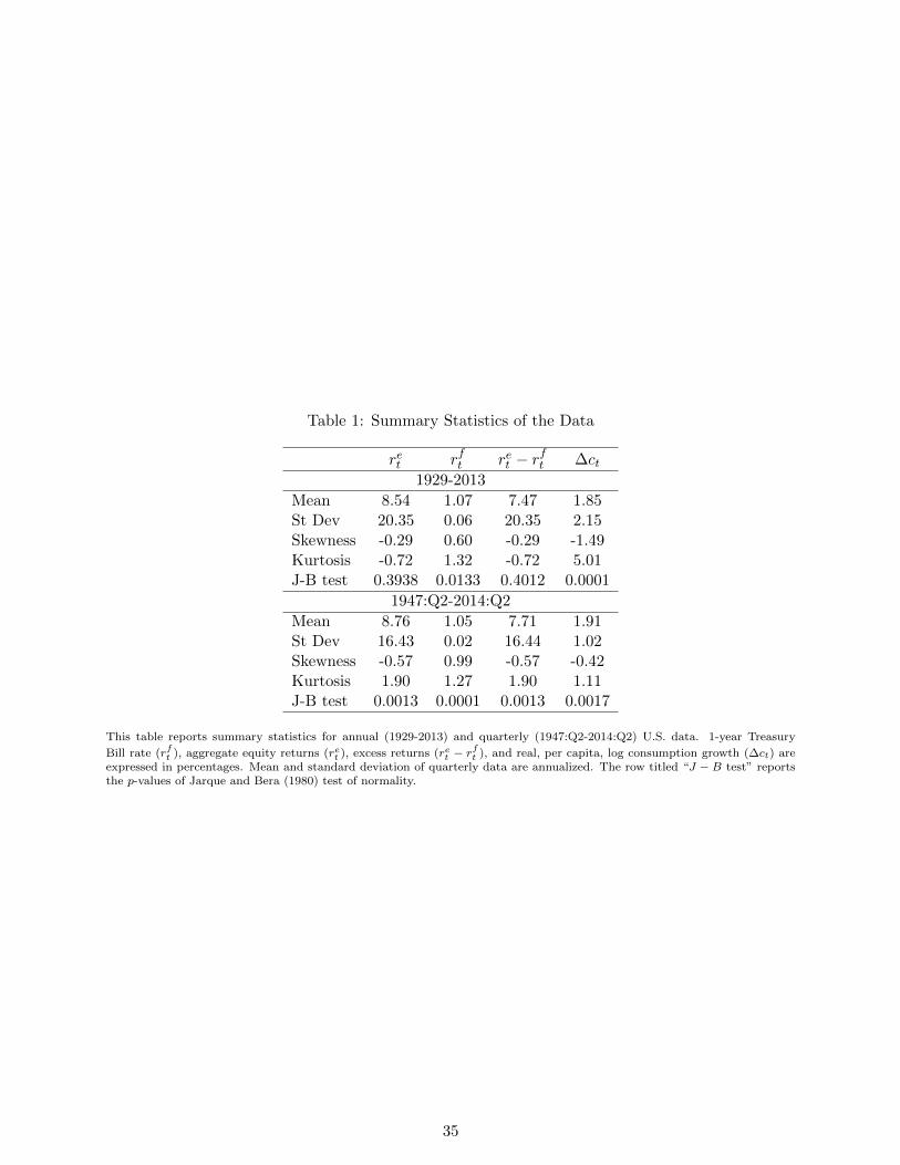
Table 1: Summary Statistics of the Data

ret rft ret − rft ∆ct

1929-2013

Mean 8.54 1.07 7.47 1.85St Dev 20.35 0.06 20.35 2.15Skewness -0.29 0.60 -0.29 -1.49Kurtosis -0.72 1.32 -0.72 5.01J-B test 0.3938 0.0133 0.4012 0.0001

1947:Q2-2014:Q2

Mean 8.76 1.05 7.71 1.91St Dev 16.43 0.02 16.44 1.02Skewness -0.57 0.99 -0.57 -0.42Kurtosis 1.90 1.27 1.90 1.11J-B test 0.0013 0.0001 0.0013 0.0017

This table reports summary statistics for annual (1929-2013) and quarterly (1947:Q2-2014:Q2) U.S. data. 1-year Treasury

Bill rate (rft ), aggregate equity returns (ret ), excess returns (ret − rft ), and real, per capita, log consumption growth (∆ct) are

expressed in percentages. Mean and standard deviation of quarterly data are annualized. The row titled “J − B test” reportsthe p-values of Jarque and Bera (1980) test of normality.

35

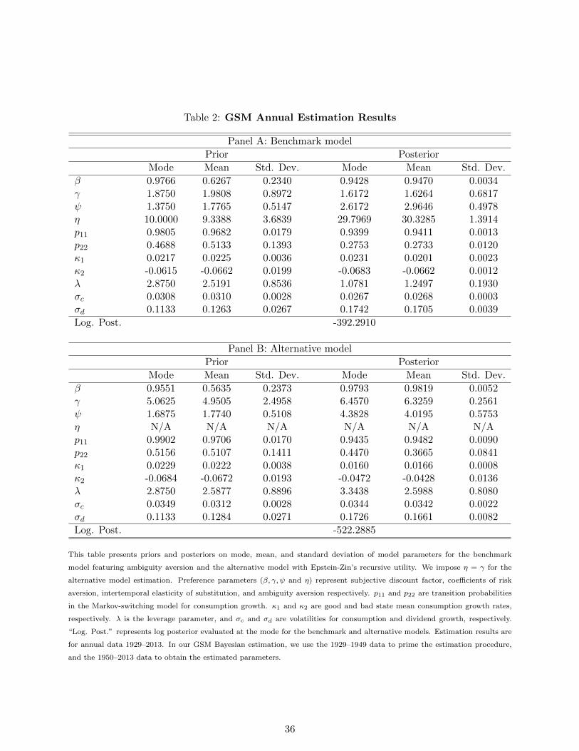
Table 2: GSM Annual Estimation Results

Panel A: Benchmark model

Prior Posterior

Mode Mean Std. Dev. Mode Mean Std. Dev.

β 0.9766 0.6267 0.2340 0.9428 0.9470 0.0034γ 1.8750 1.9808 0.8972 1.6172 1.6264 0.6817ψ 1.3750 1.7765 0.5147 2.6172 2.9646 0.4978η 10.0000 9.3388 3.6839 29.7969 30.3285 1.3914p11 0.9805 0.9682 0.0179 0.9399 0.9411 0.0013p22 0.4688 0.5133 0.1393 0.2753 0.2733 0.0120κ1 0.0217 0.0225 0.0036 0.0231 0.0201 0.0023κ2 -0.0615 -0.0662 0.0199 -0.0683 -0.0662 0.0012λ 2.8750 2.5191 0.8536 1.0781 1.2497 0.1930σc 0.0308 0.0310 0.0028 0.0267 0.0268 0.0003σd 0.1133 0.1263 0.0267 0.1742 0.1705 0.0039

Log. Post. -392.2910

Panel B: Alternative model

Prior Posterior

Mode Mean Std. Dev. Mode Mean Std. Dev.

β 0.9551 0.5635 0.2373 0.9793 0.9819 0.0052γ 5.0625 4.9505 2.4958 6.4570 6.3259 0.2561ψ 1.6875 1.7740 0.5108 4.3828 4.0195 0.5753η N/A N/A N/A N/A N/A N/Ap11 0.9902 0.9706 0.0170 0.9435 0.9482 0.0090p22 0.5156 0.5107 0.1411 0.4470 0.3665 0.0841κ1 0.0229 0.0222 0.0038 0.0160 0.0166 0.0008κ2 -0.0684 -0.0672 0.0193 -0.0472 -0.0428 0.0136λ 2.8750 2.5877 0.8896 3.3438 2.5988 0.8080σc 0.0349 0.0312 0.0028 0.0344 0.0342 0.0022σd 0.1133 0.1284 0.0271 0.1726 0.1661 0.0082

Log. Post. -522.2885

This table presents priors and posteriors on mode, mean, and standard deviation of model parameters for the benchmark

model featuring ambiguity aversion and the alternative model with Epstein-Zin’s recursive utility. We impose η = γ for the

alternative model estimation. Preference parameters (β, γ, ψ and η) represent subjective discount factor, coefficients of risk

aversion, intertemporal elasticity of substitution, and ambiguity aversion respectively. p11 and p22 are transition probabilities

in the Markov-switching model for consumption growth. κ1 and κ2 are good and bad state mean consumption growth rates,

respectively. λ is the leverage parameter, and σc and σd are volatilities for consumption and dividend growth, respectively.

“Log. Post.” represents log posterior evaluated at the mode for the benchmark and alternative models. Estimation results are

for annual data 1929–2013. In our GSM Bayesian estimation, we use the 1929–1949 data to prime the estimation procedure,

and the 1950–2013 data to obtain the estimated parameters.

36

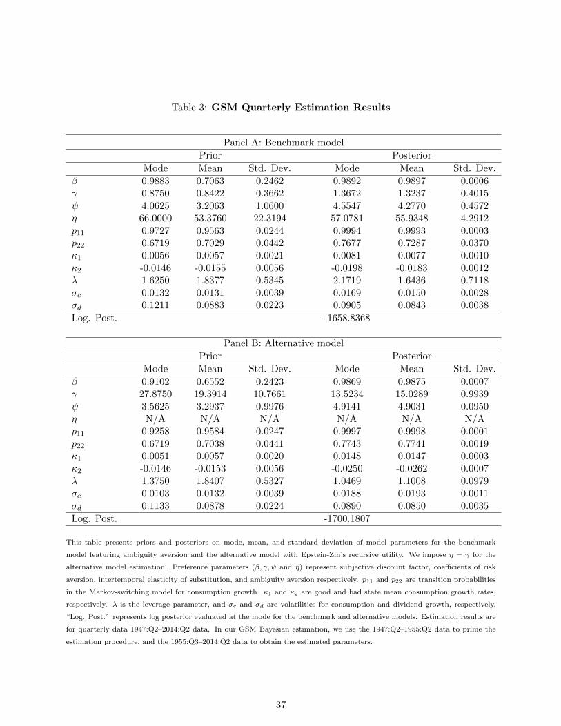
Table 3: GSM Quarterly Estimation Results

Panel A: Benchmark model

Prior Posterior

Mode Mean Std. Dev. Mode Mean Std. Dev.

β 0.9883 0.7063 0.2462 0.9892 0.9897 0.0006γ 0.8750 0.8422 0.3662 1.3672 1.3237 0.4015ψ 4.0625 3.2063 1.0600 4.5547 4.2770 0.4572η 66.0000 53.3760 22.3194 57.0781 55.9348 4.2912p11 0.9727 0.9563 0.0244 0.9994 0.9993 0.0003p22 0.6719 0.7029 0.0442 0.7677 0.7287 0.0370κ1 0.0056 0.0057 0.0021 0.0081 0.0077 0.0010κ2 -0.0146 -0.0155 0.0056 -0.0198 -0.0183 0.0012λ 1.6250 1.8377 0.5345 2.1719 1.6436 0.7118σc 0.0132 0.0131 0.0039 0.0169 0.0150 0.0028σd 0.1211 0.0883 0.0223 0.0905 0.0843 0.0038

Log. Post. -1658.8368

Panel B: Alternative model

Prior Posterior

Mode Mean Std. Dev. Mode Mean Std. Dev.

β 0.9102 0.6552 0.2423 0.9869 0.9875 0.0007γ 27.8750 19.3914 10.7661 13.5234 15.0289 0.9939ψ 3.5625 3.2937 0.9976 4.9141 4.9031 0.0950η N/A N/A N/A N/A N/A N/Ap11 0.9258 0.9584 0.0247 0.9997 0.9998 0.0001p22 0.6719 0.7038 0.0441 0.7743 0.7741 0.0019κ1 0.0051 0.0057 0.0020 0.0148 0.0147 0.0003κ2 -0.0146 -0.0153 0.0056 -0.0250 -0.0262 0.0007λ 1.3750 1.8407 0.5327 1.0469 1.1008 0.0979σc 0.0103 0.0132 0.0039 0.0188 0.0193 0.0011σd 0.1133 0.0878 0.0224 0.0890 0.0850 0.0035

Log. Post. -1700.1807

This table presents priors and posteriors on mode, mean, and standard deviation of model parameters for the benchmark

model featuring ambiguity aversion and the alternative model with Epstein-Zin’s recursive utility. We impose η = γ for the

alternative model estimation. Preference parameters (β, γ, ψ and η) represent subjective discount factor, coefficients of risk

aversion, intertemporal elasticity of substitution, and ambiguity aversion respectively. p11 and p22 are transition probabilities

in the Markov-switching model for consumption growth. κ1 and κ2 are good and bad state mean consumption growth rates,

respectively. λ is the leverage parameter, and σc and σd are volatilities for consumption and dividend growth, respectively.

“Log. Post.” represents log posterior evaluated at the mode for the benchmark and alternative models. Estimation results are

for quarterly data 1947:Q2–2014:Q2 data. In our GSM Bayesian estimation, we use the 1947:Q2–1955:Q2 data to prime the

estimation procedure, and the 1955:Q3–2014:Q2 data to obtain the estimated parameters.

37

Table 4: Financial Moments

Data Benchmark model Alternative model(1929—2013) p(η) = 10.22%

E(rft ) 1.07 0.98 1.44

σ(rft ) 0.06 0.09 0.16

E(ret − rft ) 7.47 7.31 1.36

σ(ret − rft ) 20.35 17.41 17.66

Sharpe ratio 0.37 0.42 0.08σ(Mt)/E(Mt) N/A 2.63 0.28

This table presents unconditional financial moments generated from the estimated benchmark and alternative models using

annual data. Model parameters are set at their posterior mean values reported in Table 2. E(rft ) and E(ret − rft ) are mean

risk-free rate and mean equity premium respectively, in percentage. σ(rft ) and σ(ret − rft ) are volatilities of risk-free rates and

excess returns respectively, in percentage. σ(Mt)/E(Mt) is the market price of risk.

38

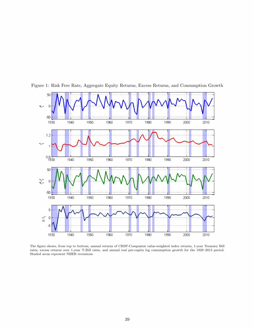
Figure 1: Risk Free Rate, Aggregate Equity Returns, Excess Returns, and Consumption Growth

The figure shows, from top to bottom, annual returns of CRSP-Compustat value-weighted index returns, 1-year Treasury Billrates, excess returns over 1-year T-Bill rates, and annual real per-capita log consumption growth for the 1929–2013 period.Shaded areas represent NBER recessions.

39

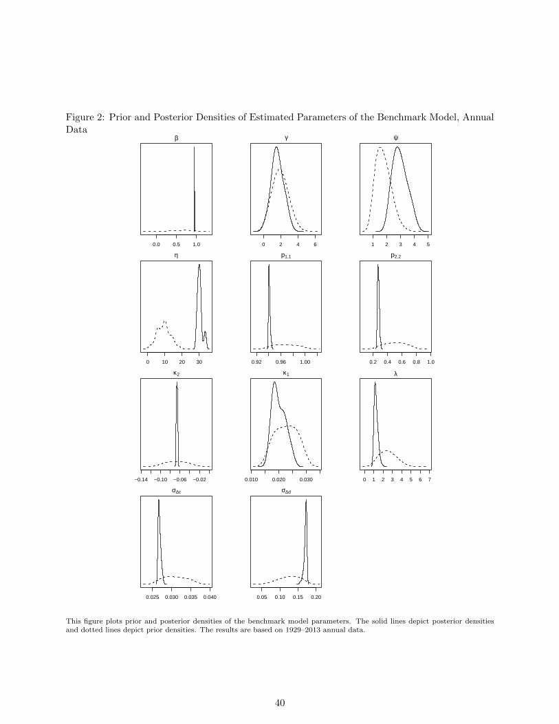
Figure 2: Prior and Posterior Densities of Estimated Parameters of the Benchmark Model, AnnualData

0.0 0.5 1.0

β

0 2 4 6

γ

1 2 3 4 5

ψ

0 10 20 30

η

0.92 0.96 1.00

p1,1

0.2 0.4 0.6 0.8 1.0

p2,2

−0.14 −0.10 −0.06 −0.02

κ2

0.010 0.020 0.030

κ1

0 1 2 3 4 5 6 7

λ

0.025 0.030 0.035 0.040

σ∆c

0.05 0.10 0.15 0.20

σ∆d

This figure plots prior and posterior densities of the benchmark model parameters. The solid lines depict posterior densitiesand dotted lines depict prior densities. The results are based on 1929–2013 annual data.

40

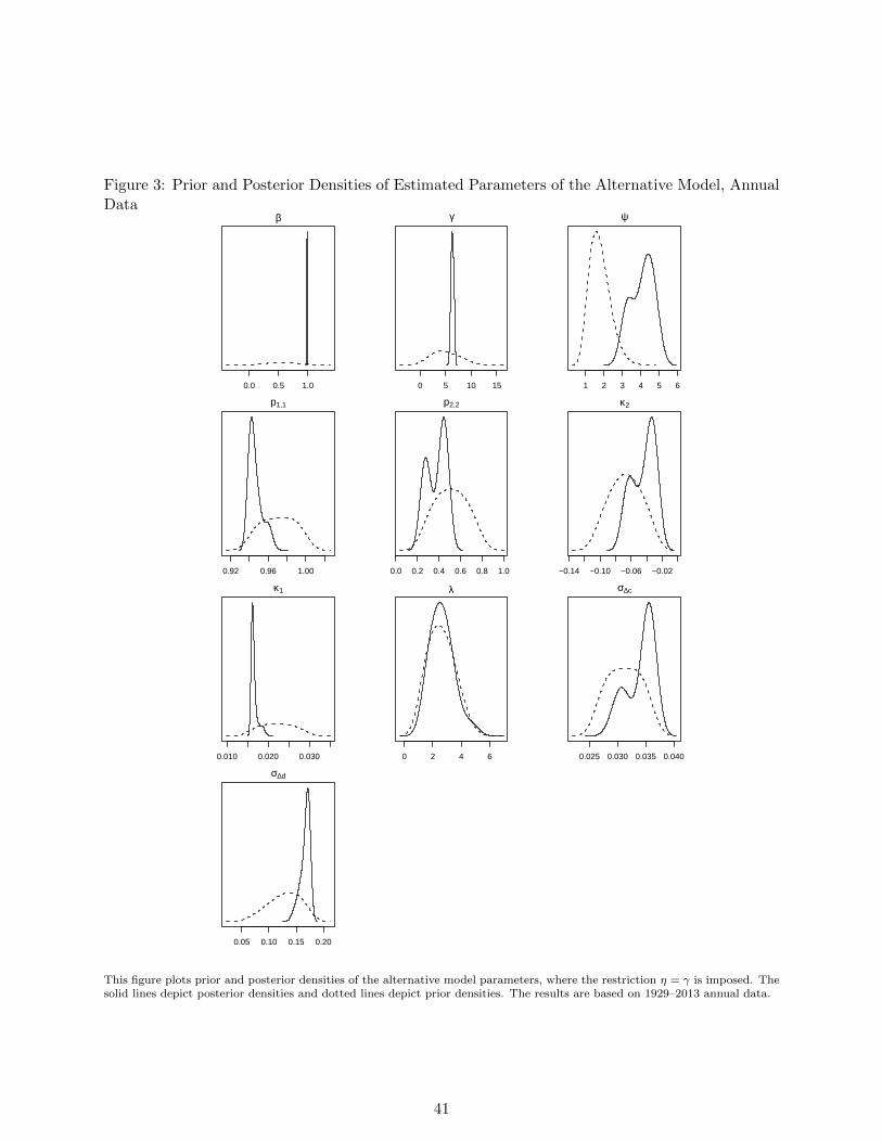
Figure 3: Prior and Posterior Densities of Estimated Parameters of the Alternative Model, AnnualData

0.0 0.5 1.0

β

0 5 10 15

γ

1 2 3 4 5 6

ψ

0.92 0.96 1.00

p1,1

0.0 0.2 0.4 0.6 0.8 1.0

p2,2

−0.14 −0.10 −0.06 −0.02

κ2

0.010 0.020 0.030

κ1

0 2 4 6

λ

0.025 0.030 0.035 0.040

σ∆c

0.05 0.10 0.15 0.20

σ∆d

This figure plots prior and posterior densities of the alternative model parameters, where the restriction η = γ is imposed. Thesolid lines depict posterior densities and dotted lines depict prior densities. The results are based on 1929–2013 annual data.

41

Figure 4: Prior and Posterior Densities of Estimated Parameters of the Benchmark Model, Quar-terly Data

0.0 0.5 1.0

β

0 1 2 3

γ

0 2 4 6

ψ

0 50 100

η

0.90 0.95 1.00

p1,1

0.60 0.70 0.80

p2,2

−0.03 −0.01 0.00

κ2

0.000 0.005 0.010 0.015

κ1

0 1 2 3 4 5

λ

0.000 0.010 0.020

σ∆c

0.02 0.06 0.10 0.14

σ∆d

This figure plots prior and posterior densities of the benchmark model parameters. The solid lines depict posterior densitiesand dotted lines depict prior densities. The results are based on 1947–2014 quarterly data.

42

Figure 5: Prior and Posterior Densities of Estimated Parameters of the Alternative Model, Quar-terly Data

−0.5 0.0 0.5 1.0 1.5

β

5 10 20 30

γ

0 2 4 6

ψ

0.85 0.90 0.95 1.00 1.05

p1,1

0.55 0.65 0.75 0.85

p2,2

−0.04 −0.02 0.00

κ2

0.000 0.010 0.020

κ1

0 1 2 3 4 5

λ

0.000 0.010 0.020 0.030

σ∆c

0.00 0.05 0.10 0.15

σ∆d

This figure plots prior and posterior densities of the alternative model parameters, where the restriction η = γ is imposed. Thesolid lines depict posterior densities and dotted lines depict prior densities. The results are based on 1947–2014 quarterly data.

43

Fig

ure

6:P

oste

rior

For

ecas

tsB

ench

mark

Mod

elA

lter

nat

ive

Model

Pre

-Gre

atR

eces

sion

For

ecas

ts

2006

2008

2010

2012

2014

2016

−10123co

nsu

mp

tio

n g

row

th

2006

2008

2010

2012

2014

2016

−100515

sto

ck r

etu

rns

2006

2008

2010

2012

2014

2016

0.00.51.01.52.0

sho

rt r

ate

2006

2008

2010

2012

2014

2016

−10123

con

sum

pti

on

gro

wth

2006

2008

2010

2012

2014

2016

−100515

sto

ck r

etu

rns

2006

2008

2010

2012

2014

2016

0.00.51.01.52.0

sho

rt r

ate

Pos

t-G

reat

Rec

essi

onF

orec

asts

2012

2014

2016

2018

2020

−10123

con

sum

pti

on

gro

wth

2012

2014

2016

2018

2020

−100515

sto

ck r

etu

rns

2012

2014

2016

2018

2020

0.00.51.01.52.0

sho

rt r

ate

2012

2014

2016

2018

2020

−10123

con

sum

pti

on

gro

wth

2012

2014

2016

2018

2020

−100515

sto

ck r

etu

rns

2012

2014

2016

2018

2020

0.00.51.01.52.0

sho

rt r

ate

Th

isfi

gu

resh

ow

sp

ost

erio

rfo

reca

sts

for

con

sum

pti

on

gro

wth

,st

ock

retu

rns,

an

dth

esh

ort

rate

for

the

pre

-an

dp

ost

-Gre

at

Rec

essi

on

per

iod

s.T

he

plo

tsare

base

don

an

nu

al

esti

mati

on

sof

the

ben

chm

ark

an

dalt

ern

ati

ve

mod

els.

Th

ed

ash

edlin

esare

the±

1.9

6p

ost

erio

rst

an

dard

dev

iati

on

s.

44

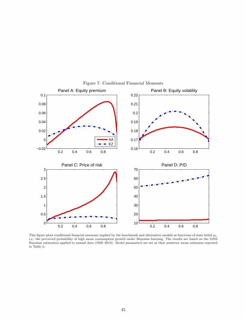
Figure 7: Conditional Financial Moments

0.2 0.4 0.6 0.8−0.02

0

0.02

0.04

0.06

0.08

0.1Panel A: Equity premium

AAEZ

0.2 0.4 0.6 0.80.16

0.17

0.18

0.19

0.2

0.21

0.22Panel B: Equity volatility

0.2 0.4 0.6 0.80

0.5

1

1.5

2

2.5

3Panel C: Price of risk

0.2 0.4 0.6 0.810

20

30

40

50

60

70Panel D: P/D

This figure plots conditional financial moments implied by the benchmark and alternative models as functions of state belief µt,i.e., the perceived probability of high mean consumption growth under Bayesian learning. The results are based on the GSMBayesian estimation applied to annual data (1929–2013). Model parameters are set at their posterior mean estimates reportedin Table 2.

45

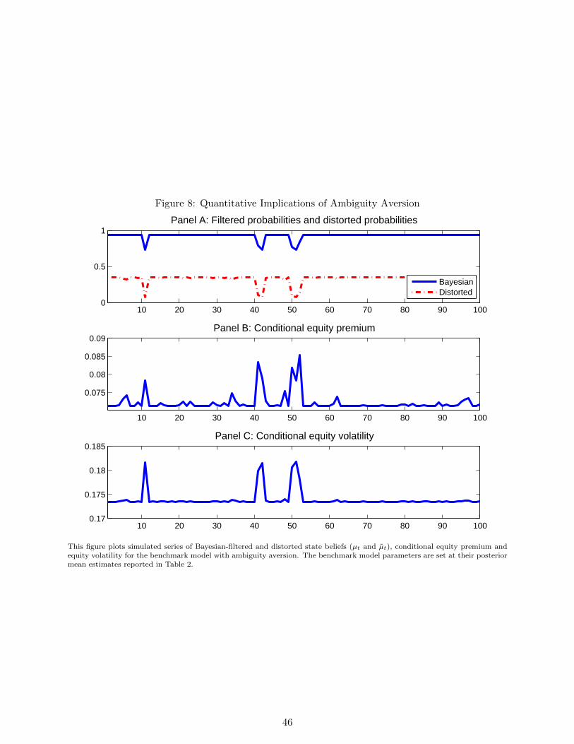
Figure 8: Quantitative Implications of Ambiguity Aversion

10 20 30 40 50 60 70 80 90 1000

0.5

1Panel A: Filtered probabilities and distorted probabilities

BayesianDistorted

10 20 30 40 50 60 70 80 90 100

0.075

0.08

0.085

0.09Panel B: Conditional equity premium

10 20 30 40 50 60 70 80 90 1000.17

0.175

0.18

0.185Panel C: Conditional equity volatility

This figure plots simulated series of Bayesian-filtered and distorted state beliefs (µt and µt), conditional equity premium andequity volatility for the benchmark model with ambiguity aversion. The benchmark model parameters are set at their posteriormean estimates reported in Table 2.

46