Finance and Welfare: The Effect of Access to Credit

on Family Structure

Isaac Hacamo∗

October, 2014

There is a large debate over the welfare effects of the early 2000s housing boom and bust. Onepotentially important welfare effect is the impact of mortgage credit expansion on family structure.I exploit zip code level variation within US counties to study the effect of access to credit onfertility outcomes through a channel associated with a more efficient reallocation, which allowsyoung households to access space by either moving to larger homes or achieving homeownershipearlier in their life-cycle. To causally estimate this effect, I compare, within the same county, zipcodes that have the same level of old (age>65) population, but have different levels old homeownerswho live alone. I show that from 2000 to 2006, there is a disproportional increase in mortgagesoriginated and sold relative to non-sold in zip codes with many old homeowners who live alone,despite no difference from 1995 to 2000. I estimate that between 330,000 and 480,000 babies wereborn between 2000 and 2006 because of the reallocation channel. I present suggestive evidencethat the majority of this effect might have been a life-cycle rather than a life-time effect, younghouseholds shifted their fertility decision in their life-cycle. This evidence would explain part of thelarge drop in fertility observed during the financial crisis as a correction after the housing boom.

∗Assistant Professor, Finance Department, Kelley School of Business, Indiana University. Email: ihacamo@

indiana.edu. An earlier version of this paper is part of my PhD dissertation at UC Berkeley. I thank AnnetteVissing-Jørgensen, Adair Morse, Atif Mian, and Enrico Moretti for their generous support and guidance during mydissertation. For valuable comments and discussions, I also thank Vladimir Asriyan, Brian Ayash, Christopher Bar-rett, Mathew Botsch, Mark Garmaise, Brett Green, Nandini Gupta, Marcel Fischer, Ryan Firestone, Samuli Knupfer,Geng Li, Crocker Liu, Jesper Lund, Gustavo Manso, Terrance Odean, Iyer Rajkamal, Tomas Reyes, Gisela Rua, An-gelique Saavedra, Victoria Vanasco, Nancy Wallace, Ingrid Werner and seminar participants at UC Berkeley, Boardof Governors of the Federal Reserve System, Indiana University, The Ohio State University, Cornell University, CaseWestern Reserve University, and Copenhagen Business School. I gratefully acknowledge the financial support of theWhite Foundation and Pinto-Fialon Fund during my dissertation.

I INTRODUCTION

The topic of access to finance and welfare has been studied in a number of dimensions. For

example, studies have sought to quantify the impact of access to finance on welfare via its effects on

intertemporal consumption smoothing (Jappelli and Pistaferri 2011; Gertler, Levine, and Moretti

2009), college enrollment (Levine and Rubinstein 2013), and job choices after graduation (Shu

2013). Others have studied the welfare impact of finance by documenting returns to finance jobs

(Philippon and Reshef 2012; Kaplan and Rauh 2010), the elasticity of income with respect to

financial output (Philippon and Reshef 2013), and borrower’s behavior associated with distress

finance (Melzer 2011; Karlan and Zinman 2010; Morse 2011).

In this paper, I introduce a new channel whereby access to credit can offer welfare improvements,

namely in fertility outcomes.1 Given that space and children are likely to be strong complements,

the increase in the availability of mortgage credit during the U.S. housing boom, which is associated

with a large increase in homeownership and home transactions, could have had a large impact

on households’ decisions to have children. This is because demographers have suggested that the

transition from renting to homeownership is associated with an increase in fertility, arguably because

households have access to more space (Felson and Solaun 1975; Kulu and Vikat 2007; Mulder and

Billari 2010; Strom 2010). It is then possible that sizable changes in the number of births might have

occurred due to the expansion of mortgage credit, allowing me to plausibly identify a causal effect

of access to credit on fertility decisions. In short, the contribution of this paper is the identification

and quantification of an effect of access to credit on fertility decisions through a channel associated

with a more efficient reallocation of the existing housing stock among households, which creates

access to space and for young households who want to expand their families.

The identification of the effect of access to credit on fertility outcomes relies on the ability to

isolate a reallocation channel — associated with access to space — from other causes of fertility

choices such as changes in household permanent income or changes in housing wealth. I do this

1To make this argument, it must be assumed that fertility choices are, on average, welfare-improving. Beyondrevealed preference demographers commonly link fertility and welfare, e.g., Thomson and Brandreth (1995); Kohler,Behrman, and Skytthe (2005); Margolis and Myrskyla (2011). I proceed under the assumption that having childrenis welfare-improving.

1

by laying out three channels by which the housing market could affect fertility: a wealth channel

and two space channels. The house wealth channel helps households who are homeowners finance

child rearing. Dettling and Kearney (2011) study the effect of house wealth on household fertility

decisions; using Metropolitan Statistical Area level house prices from 1996 to 2006, they find

that a $10,000 increase in house prices is associated with a 0.8% increase in fertility rates across

homeowners (5%) and renters (-2.4%). The space channels, on the other hand, make it feasible

to accommodate another house member in the dwelling, and are associated with access to larger

homes or first-time homeownership. The two space channels through which access to credit impacts

fertility are new construction and more efficient reallocation of the housing stock among households.

My goal is to isolate the space channel associated with reallocation as a new causal channel

between access to credit and fertility. To this end, I first estimate, after controlling for the observable

determinants of fertility2 and including county effects, the three housing channels in an ordinary

least squares (OLS) framework. I proxy the intensity of reallocation associated with the expansion of

credit supply by using the change in mortgages originated and sold—not kept in the lender’s balance

sheets. However, some mortgage origination is not associated with reallocation. By choosing an

appropriate instrument and using a two-stage least squares (2SLS) approach, I isolate the mortgage

origination associated with reallocation and address endogeneity concerns from the OLS estimation.

Although the OLS estimates reveal that the reallocation is the relevant housing channel, the

OLS estimates can be biased in both directions. For example, male permanent income shocks relax

households’ budget constraint allowing them to fund child rearing and simultaneously obtain more

easily a mortgage loan. In this case, the OLS estimates are biased upwards if permanent income

cannot be precisely controlled. Conversely, a shock to the female’s level of education, or potential

labor income, creates a negative bias, since the female’s opportunity cost of child rearing increases,

while the chance of qualifying for a mortgage loan increases. Therefore, to credibly identify the

effect of access to credit on households’ fertility decisions through a reallocation channel, I need an

instrumental variable that correlates with fertility through the channel of interest — reallocation

2Joseph Hotz et al. (1997) survey the fertility literature in developed economics and report the following variablesas the most well identified determinants of fertility: income, unemployment, wealth, education, age structure, race,and ethnicity.

2

— and not through any other unobservable factor that drives fertility.

The empirical design is defined by four features. First, I assume that, between 2000 and 2006,

the whole U.S. economy experienced an outward shift on supply of credit led by relaxation of credit

standards (Mian and Sufi 2009; Keys, Mukherjee, Seru, and Vig 2010, Adelino, Schoar, and Severino

2012, Di Maggio and Kermani 2014). Second, to control for geographical differences between cities,

especially differences in labor and housing markets that could confound the identification, I include

county effects in all estimations, hence only the zip code level variation within-county is used for

identification. Third, I use zip code level variation in the fraction of homeowners who are older

than 65 and live alone in 2000 as an instrument, henceforth old homeowners, to generate plausible

exogenous variation in the supply of houses that could easily be subject to reallocation. Fourth,

I control for the fraction of population in the county who is older than 65 in 2000. This way, the

empirical exercise consists in comparing the changes from 2000 to 2006 in two zip codes in the

same county, with the same fraction of old population, but different levels of old homeowners who

live alone. In a more conservative specification, I also include the fraction of homeowners who live

alone and are older than 75. In this conservative specification, I aim to control for the natural

reallocation that happens in the economy regardless of the expansion of credit supply, and thus

provide a conservative estimation of the effect of access to credit on fertility outcomes.

The source of variation of the instrument relies on the underlying motives that old households

have to exit their houses. During the housing boom, old homeowners exited their houses because

they could monetize their home values, could not afford to pay increasing property taxes, or suf-

fered from age-related health adversities such as death or disability. I claim that the exit due to

monetization and increasing property taxes is driven by the global increase in house prices that

was caused by the credit supply shock. Some old homeowners have a reservation price for their

houses that credit constrained households can only pay when credit standards are loosened. Other

old homeowners sell their houses and move out of their neighborhood when, due to increases in

property assessments induced by the credit boom, property taxes rise to unaffordable levels relative

to their income. The exit due to age-related health adversities is independent of the credit supply

shock. Between 2000 and 2006 and within-county, the change in mortgage origination per capita

3

is much larger in zip codes with high fraction of old homeowners relative to zip codes with low

fraction of old homeowners, implying that the rank condition is met. Moreover, the increase in

homeownership for young households (age<44) and decrease in homeownership for old households

(age>65) is also larger in zip codes with high fraction of old homeowners.

The instrument then isolates mortgage origination associated with reallocation of young house-

holds with old homeowners who live alone. By projecting the change in mortgage origination per

capita on the instrument defined as old homeowners, the first stage will pick up mortgage origina-

tion that is associated with reallocation.3 The exclusion restriction is guaranteed by two conditions.

First, young households move into to houses of old homeowners who live alone because of the easier

access to credit, and not due to self-selection motives associated with other determinants of fertil-

ity, such as increases in unobservable permanent income. Second, the within-county zip code level

variation of old homeowners who live alone in 2000 is not confounded by an omitted variable, such

as unobservable school quality, which would consistently predict higher fertility outcomes in these

zip codes regardless of an easier access to credit. To ensure that the exclusion restriction is met, I

introduce a more conservative empirical design that controls for the level of old homeowners who

live alone and are older that 75. Since the average life expectancy in the U.S. is 76 years for males

and 81 years for females, shifting the age limit to 75 years old, increases the weight on the exit due

to health-related reasons, a ‘natural’ reallocation mechanism. Hence, by attempting to control for

‘natural’ reallocation, the effect captured by the variation of homeowners who live alone and are

older than 65 will not be contaminated by self-selection motives.

One may still be concerned with the exclusion restriction of the aforementioned identification,

particularly because unobservable income innovations could drive housing demand of young and

credit constrained households and consequently lead them to purchase homes of old homeowners,

regardless of the credit supply shock.

If the effect of access to credit on fertility is driven by other factors that are not associated to the

credit supply shock, it is plausible that the same effect will also be present before the expansion of

mortgage credit, in particular from 1995 to 2000, a period when the US economy experienced high

3I assume that within-county houses are on average larger than apartments and thus suitable for young householdsto form and expand their families. I present anecdotal evidence in section III.a that supports this assumption.

4

income growth and house price growth. One can conduit two tests. First, during the period from

1995 to 2000, does per capita mortgage origination changes faster in zip codes with old homeowners

who live alone? Second, during the period from 1995 to 2000, does per fertility changes faster in zip

codes with old homeowners who live alone? If the impact of the instrument on fertility is zero when

the credit induced reallocation channel is turned off, it will lend more confidence to the exclusion

restriction. The answer to the both questions is no.There is no relative difference in mortgage

origination from 1995 and 2000 in zip codes with old homeowners who live alone. There is no

difference in fertility changes during this period in zip codes with old homeowners who live alone.

During a period when the first stage fails, the instrument has no effect on the outcome variable.

To conduct my empirical analysis I construct a dataset of zip code level data that draws from a

variety of data sources. I collect data on births from 11 Departments of Public Health: California,

Idaho, Indiana, Florida, Kansas, New York, Massachusetts, Oregon, South Carolina, Texas, and

Wisconsin. I use individual loan data from Home Mortgage Disclosure Act (HMDA) to compute

mortgage origination at the zip code level, and use income data from the Internal Revenue Service

(IRS) to compute per capita income growth. I use data extracted from Zillow to compute zip

code level house prices growth and use the Census and American Economic Survey to compute the

demographic variables. The final dataset encompasses 2,717 zip codes, and covers approximately

70 million people in 2000, approximately 25% of the total U.S. population.

My estimates of the three housing channels show that between 2000 and 2006, the house wealth

had a negligible effect on fertility, the construction channel had a negative effect on fertility, and the

reallocation had a large and positive effect on fertility. A one standard deviation increase in new

construction leads to a 1.8% decline in fertility from 2000 to 2006. The negative sign suggests that

new construction is associated with older households who have passed the fertility age. Dettling and

Kearney (2011) find that a $10,000 increase in house prices is associated with a net annual increase

of 0.8% in fertility rates. One possible explanation for this difference could rely on the heterogeneity

of house price growth across metropolitan areas between 1996 and 2006, since in contrast with the

early 2000s, house price growth from 1996 to 2000 happened mainly in geographies with high

income growth (Glaeser, Gottlieb, and Tobio 2012; Ferreira and Gyourko 2011). Dettling and

5

Kearney (2011)’s results could be drawing from the beginning of the sample, while mine draw from

the second part of the time period they analyze. I present suggestive evidence that this is the case.

Changes in fertility from 1995 to 2000 are strongly correlated with contemporaneous house price

growth, while no statistical relationship exists from 2000 to 2006.

By contrast, the reallocation of the existing housing stock has a larger impact, a one standard

deviation increase in reallocation leads to a 4.6% to 7% increase in fertility from 2000 to 2006, which

represents 20% to 30% of the standard deviation of fertility change from 2000 to 2006. Based on

these coefficients, I estimate the aggregate effect of the credit induced reallocation channel. I

estimate that approximately 330,000 to 480,000 new births occurred during the housing boom due

to the reallocation channel.

Such a large increase in the number of births begs the question on how much of this increase was

a life-time change, a permanent change in the number of births, or a life-cycle change, a change in

the timing when households choose to have children. Both cases are important, but have different

implications in the economy. To understand the nature of the change in the number of births, I

study the fertility changes after the housing boom, from 2006 to 2010. If the increase in fertility

during the housing boom was a life-time change, no relative difference should exist between high and

low old homeowners zip codes after the housing boom. On the other hand, if the change in fertility

during the housing boom was a life-cycle change, then a correction in fertility outcomes should be

observable after the housing boom. Using a similar empirical design as explained above, I show

that, between 2006 and 2010, zip codes that experienced high levels of credit induced reallocation

were more likely to experience large drops in fertility outcomes. The drop is of the same size than

the increase, implying that the increase in fertility during the housing boom was undone during the

financial crisis. Although the empirical design is not ideal because it does not control for several

other channels that might have impacted fertility outcomes during the financial crisis, the current

results point in the direction of a full life-cycle change rather than a life-time change.

The remainder of this section presents the literature related to this paper. The next section

outlines the dataset used in this paper, its construction, and summary statistics. Section III presents

the empirical methodology, namely the housing-related mechanisms. Section III also lays out the

6

empirical design to explore the causal effect of access to finance on fertility decisions through the

reallocation channel. OLS and IV results are in the first part of section IV. The second part of

section IV presents robustness tests and the analysis of female participation in the labor force

during the financial crisis. Finally, section V reports concluding remarks.

Related Literature. This paper relates to two strands of literature. Firstly, it relates to the

literature that studies the implications of the mortgage credit expansion and its welfare effects.

Mian and Sufi (2009) and Keys, Mukherjee, Seru, and Vig (2010) seminal works show that in the

beginning of the 2000s the U.S. economy experienced an outward shift in the supply of credit. Mian

and Sufi (2009) document that less creditworthy borrowers experienced easier access to mortgage

credit despite their negative income growth. Keys, Mukherjee, Seru, and Vig (2010) suggest that

existing securitization practices adversely affected the screening incentives of subprime lenders.

Adelino et al. (2012) use exogenous changes in the conforming loan limit as an instrument for lower

cost of financing and higher supply to show that easier access to credit significantly increases house

prices. Motivated by these findings and the severity of the financial crisis, a subsequent literature

started examining the welfare effects of the expansion of credit and the role of finance in the

past decades. Greenwood and Scharfstein (2013) show that, starting in 1980, fees associated with

residential mortgages became a sizable portion of the growth in the U.S. financial services industry,

while Philippon and Reshef (2012) show that workers in finance earned an education-adjusted wage

premium of 50% in 2006, despite no premium in 1990. Charles, Hurst, and Notowidigdo (2013)

suggest that housing booms disguise unemployment growth as they reduce the likelihood that

displaced manufacturing workers remain unemployed. Mian and Sufi (2012) find that geographical

differences in household debt overhang explain the differences of cross-sectional unemployment

in the non-tradable sector. Levine and Rubinstein (2013) present evidence that intrastate bank

deregulation increases the probability to attend college for individuals with particular learning

abilities and family traits. Shu (2013) shows that careers in finance, especially at hedge funds and

trading positions, attract students with high raw academic talent. This paper adds to this literature

by highlighting another welfare dimension that was affected by the expansion of mortgage credit -

the family structure.

7

Secondly, this paper relates to the vast literature that studies the determinants of fertility. More

than two centuries ago Malthus (1798) predicted a positive relation between income growth and

population growth based on the hypothesis when people’s incomes are higher they form families

earlier and have more children. However, cross-national evidence over the last hundred years

contradicts this prediction. As nations became industrialized and as their incomes increased, the

fertility rate went down. Becker (1960), Becker and Lewis (1973) and Willis (1973) introduce the

distinction between the quality and the number of children to explain the negative correlation

between income and fertility. Angrist et al. (2010), however, show no evidence of a quantity-

quality trade-off. Mincer (1963), Becker (1965), Willis (1973) and Schultz (1985) introduce women’s

time allocation decisions and emphasize the opportunity costs of women’s time. Ermisch (1989)

introduces market price of childcare to explain the impact of the mother’s wage. Adsera (2005)

suggests that the negative trend in fertility in developed countries is associated with constraints of

the labor market where fertility decisions are taken. The cyclical behavior of fertility has received

much attention since the work of Butz and Ward (1979). In most countries the fertility rate shows

a negative response to unemployment along the business cycle, i.e., fertility is procyclical. Galor

and Weil (1996) present a model where increases in women’s wages lead to a decrease in fertility

rates. Dettling and Kearney (2011) is the closest work to this paper. They use MSA house price

variation to study the effect of house wealth effect on fertility decisions from 1996 to 2006. This

paper reconciles their evidence with the other housing channels and highlights the importance of

reallocation that stems from the relaxation of credit constraints.

II DATA

II.a Macroeconomic Indicators

Before discussing the micro dataset used in the empirical analysis, I show that, in the last 20

years, the relationship between mortgage origination and fertility is present in the aggregate data

only during the housing boom. The top panel in Figure 1 shows that the aggregate number of births

in the U.S. started an uptrend in 1996 that lasted until the end of the housing boom. The middle

8

panel shows that, over the same time period, the fertility rate4 exhibited an uptrend between 2000

and 2007. Both time-series suggest a shift in fertility choices during the housing boom period.

The bottom panel of Table 1 shows that the annual volume of mortgage origination for home

purchase shifted to a higher level between 2000 and 2006. Figure 2 confirms that households used

mortgage loans to purchase existing and newly constructed houses by showing that the number of

home transactions increased faster between 2000 and 2006. Figure 2 also shows that the number

of transactions of existing houses was significantly larger than the number of newly constructed

houses. This difference suggests that during the housing boom households were more likely to

move into an existing house than a newly constructed one. Figure 3, using county-level data,

proceeds to investigate the potential relationship between access to credit and fertility by showing

that since 1995 mortgage origination and fertility are only positively correlated in changes between

2000 and 2006. The absence of correlation from 1995 to 2000, a period of strong economic growth,

raises the bar for the permanent income hypothesis to be a credible alternative hypothesis. In

order for permanent income to explain the positive correlation between fertility change and per

capita mortgage origination change from 2000 to 2006 the correlation of income growth and per

capita mortgage origination change would need to change from 1995-2000 to 2000-2006. A different

flavor of the same argument is delivered by Figure 4. Figure 4 sorts counties on the per capita

mortgage origination change from 2000 to 2006 and depicts the time series of the fertility rate

for the top and bottom quintiles between 1990 and 2010. Prior to 1996, fertility rates are not

statistically different between the two groups. By 2000, the difference is small; however, between

2000 and 2006, fertility rates increased rapidly in high mortgage origination counties; yet, in low

mortgage origination counties fertility rates remained fairly constant. Lastly, Figure 6 shows that

between 2000 and 2005, young households experienced large gains in homeownership , while older

households experienced small or no gains in homeownership. This pattern is however not present in

the data from 1990 to 1995. In sum, the macro evidence suggests that access to credit was strongly

associated with fertility decisions during the credit boom.

4According to the CDC, fertility rate is defined as the number of births divided by the number of women in childbearing age, assumed to be from 15 to 44 years old.

9

II.b Micro Data

I draw from a variety of data sources to construct the sample used in this paper. The sample

consists of data on births, loans, income, house prices, employment, and demographics. Data on

births is available by county and zip code, and was collected from the Department of Public Health

(DPH) of each state. Birth statistics at the county level are available for 48 states from 2000

to 2006.5. I only use the county data to estimate the macro impact in change in fertility. Birth

statistics at zip code level is available for 11 states: California, Idaho, Indiana, Florida, Kansas, New

York, Massachusetts, Oregon, South Carolina, Texas, and Wisconsin. For confidentiality reasons,

in some states birth statistics are not available when the number of births is smaller than five in a

given geography. Data at the zip code level is available for years 1995, 2000 and 2006.

Home Mortgage Disclosure Act (HMDA) provides loan level data from 1990 to 2011. Loan level

data is publicly available for lenders that meet a disclosure criteria defined by HMDA every year.

Each loan application provides information on year of application, lender, type of loan, loan amount,

action taken by the lender, reason for denial, in case the loan is denied, race, sex and income of

the applicant and co-applicant, census tract, county FIPS, and state FIPS where the loan was

originated, owner occupancy, and purpose. Loans have four types of purpose: home purchase, home

improvement, refinancing, and multifamily dwelling. I only use loans that are originated for home

purchase and are owner-occupied as principal dwelling.

I use the Internal Revenue Service (IRS) data to compute the zip code level income per capita.

The IRS provides zip code level data for years 2001 and 2006. The provided income data includes

adjusted gross income, number of returns, and wage income. Income per capita is defined as the

ratio of the adjusted gross income to the number of returns.

Home prices are from Zillow. I extracted their sales-price-based price index for zip codes that

have sufficient transaction level. Each Zillow Home Value Index (ZHVI) is a time series tracking

the monthly median home value in a particular geographical region. In general, each ZHVI time

series begins in April 1996. Instead of using a repeat sales methodology, Zillow uses the same

underlying deed data as the Case-Shiller index but creates a hedonically adjusted price index. The

5The DPH of the state of Delaware and Louisiana did not make available their data at county level.

10

Zillow index uses detailed information about the property, collected from public records, including

the size of the house, the number of bedrooms, and the number of bathrooms. To the extent that

the average measured characteristics of the home change over time, the Zillow index will capture

such changes.6 Guerrieri, Hartley, and Hurst (2013) show that the correlation between Case-Shiller

Index and Zillow Index where the two samples overlap is equal to 94%. Monthly home prices are

available from 1996 to 2012 for 10,187 zip codes.

Data on number of hospitals per capita is from the County of Business Patterns (CBP) annual

survey. CBP provides total employment for all establishments located in a given zip code broken

down by NAICS five industries codes.

Zip code school scores were obtained from Global Report Card. Reading and math scores are

available for each school district from 2004 onwards. I use the reading score level in 2004 as a

measure of the school district quality. I map zip codes to school districts to obtain a zip code level

measure of school quality.

Finally, I use the public data from the Decennial Census and the American Economic Survey to

obtain zip code data on gender, race, ethnicity, type of household, educational attainment, housing

tenure, and number of bedrooms. The 2000 Decennial Census provides zip code data directly. On

the other hand, to access the zip code data from the ACS, one needs to use 5-year averages. I use

the ACS’s 5-year averages from 2005 to 2009.

The construction of the dataset proceeds as follows: I start by merging the births and the Zillow

Price data. The merged data set covers 3,256 zip codes. I proceed to merge it with HMDA data,

and the number of merged zip codes drops to 2,825. I then merge it with the IRS data and the

CBP data, and as a result the number of zip codes drops to 2,793. Finally, after merging with

the Census and ACS dataset the number of zip codes is 2,792. I then drop data points where

births are missing in either 2000 or 2006, and repeat the same criteria for house prices and income

data. The resulting dataset encompasses 2,717 zip codes, and covers 68.3 million people in 2000,

approximately 25% of the total U.S. population.

6More information about the computation methodology of the Zillow home price index can be found here:http://www.zillow.com/blog/research/2012/01/21/zillow-home-value-index-methodology/.

11

Summary Statistics

Table 1 presents the summary statistics of the variables presented in this section. The average

change in per capita mortgage origination between 2000 and 2006 was 0.64 per 1000 people on

average, while the change in mortgages that were originated and sold during the same period was

1.71 per 1000 people, and the change in mortgages that were originated but not sold was -1.07 per

1000 people. This is consistent with the evidence that, during the housing boom, lenders increased

origination and securitization (Mian and Sufi 2009; Keys, Mukherjee, Seru, and Vig 2010). The

average house price growth from 2000 to 2006 was 107%, 12.8% in annualized terms. For the 6 year

period of analysis, the per capita income growth was 22%, or 3.3% in annualized terms. Change

in the female unemployment rate from 2000 to 2006 was 1.1%. Fertility changed by 3.37 per 1000

women in child bearing age from 2000 to 2006. The change in the zip code fraction of Hispanics

and Blacks was on average 2.8% and 0.33%, respectively. The average zip code population in 2000

was 24,846.

III EMPIRICAL METHODOLOGY

III.a Mechanism

If households are credit constrained, an outward shift in the supply of mortgage credit induces

them to adjust their housing consumption. As a result, households move within the existing housing

stock as well as to newly constructed houses. They access more space, as renters become first-time

homeowners and existing homeowners move into larger or better quality houses. I assume that

the transition from renting to homeownership provides households additional housing space.7 The

credit supply shock then provides households access to space that would have been unaccessible

otherwise or would have only been reachable later in their life-cycle. As households access more

space, they presumably change their consumption of complementary goods; specifically, if they

7I assume that the supply of apartments with more than two bedrooms is thin. Using 30 million Craigslist adsfrom 2008 to 2013, Figure 5 presents suggestive evidence of thinness in the rental market. The price difference froma one to two bedroom is on average $390. By contrast, the price difference from a two to three bedroom apartmentis $1100, and from a three to four bedroom is $2220. The higher relative increase in rent prices for larger apartmentssuggests short supply of large dwellings in the U.S. rental market.

12

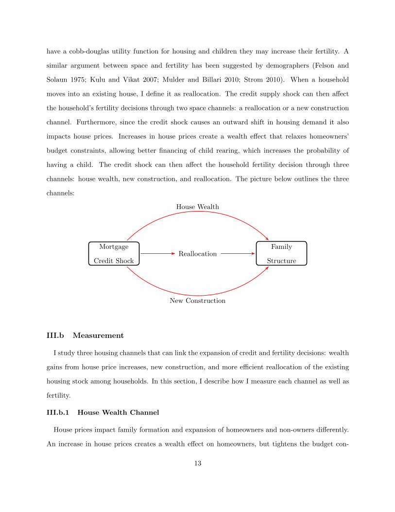
have a cobb-douglas utility function for housing and children they may increase their fertility. A

similar argument between space and fertility has been suggested by demographers (Felson and

Solaun 1975; Kulu and Vikat 2007; Mulder and Billari 2010; Strom 2010). When a household

moves into an existing house, I define it as reallocation. The credit supply shock can then affect

the household’s fertility decisions through two space channels: a reallocation or a new construction

channel. Furthermore, since the credit shock causes an outward shift in housing demand it also

impacts house prices. Increases in house prices create a wealth effect that relaxes homeowners’

budget constraints, allowing better financing of child rearing, which increases the probability of

having a child. The credit shock can then affect the household fertility decision through three

channels: house wealth, new construction, and reallocation. The picture below outlines the three

channels:

Family

StructureReallocation

Mortgage

Credit Shock

House Wealth

New Construction

III.b Measurement

I study three housing channels that can link the expansion of credit and fertility decisions: wealth

gains from house price increases, new construction, and more efficient reallocation of the existing

housing stock among households. In this section, I describe how I measure each channel as well as

fertility.

III.b.1 House Wealth Channel

House prices impact family formation and expansion of homeowners and non-owners differently.

An increase in house prices creates a wealth effect on homeowners, but tightens the budget con-

13

straint for renters since it increases the cost of housing. To distinguish the effect on homeowners

and renters, Dettling and Kearney (2011) use a specification that interacts the house price growth

and the initial level of homeownership, since the house price effect is larger in zip codes where the

level of homeownership is larger. This specification is useful when one wants to separate the house

price effect on renters and homeowners. In the context of this paper, it is only relevant to measure

the aggregate effect of house prices, therefore, the measure of house wealth for a zip code i is simply

the house price growth measure as:

House Wealth Measure 2000→2006,i =House Prices 2006,i − House Prices 2000,i

House Prices 2000,i

where HP Growth is measured as the growth in the zip code level Zillow Price Index.

III.b.2 Construction Channel

An exogenous shock in new construction affects house prices and housing consumption. House

prices are affected through a pure supply channel. The effects on housing consumption depend on

the relative size and quality of new houses constructed. To capture the space effect created by new

construction, I use the growth in the total number of housing units:

Construction Measure 2000→2006,i =#House Units 2006,i − #House Units 2000,i

#House Units 2000,i

where house units are measured using the Census data and the American Community Survey.

III.b.3 Reallocation Channel

Credit constrained households have below optimal housing consumption. A credit supply shock

that lowers the lending standards facilitates the reallocation of housing resources. In the event of a

credit supply shock, zip codes that experience large increases in mortgage origination are likely to

experience high levels of reallocation. The ideal measure of reallocation quantifies the number of

houses that are bought by credit constrained households from homeowners who were underutilizing

their house. Since such measure is not available an alternative proxy for reallocation during a

14

period of credit expansion is the change in per capita mortgage origination:

Reallocation Measure 2000→2006,i =

[# Mortgage Origination

# Population

]2006,i

−[

# Mortgage Origination

# Population

]2000,i

One potential shortcoming is that the increase in origination may not be associated with the

shock in the supply of credit, although very correlated as shown by Mian and Sufi (2009). One

potential improvement is to refine the above measure to mortgages that were originated and sold.

Since it has been widely shown that, during the housing boom, the ability to not keep loans in the

lender’s balance sheets was one of the key features of the expansion of credit (Keys et al. 2010).

Therefore an alternative measure for credit induced reallocation is:

Reallocation Measure 2000→2006,i =

[# Mortgages Originated & Sold

# Population

]2006,i

−[

# Mortgages Originated & Sold

# Population

]2000,i

The increase in mortgages that were originated and sold is likely to be negatively correlated with

the decrease of mortgages kept in-house. However, all else equal, the variation in mortgages not

sold and kept in-house is informative. Hence, a third alternative measure for the credit induced

reallocation is:

Reallocation Measure 2000→2006,i =

[# Originated & Sold − Originated & Non Sold

# Population

]2006,i

−[

# Originated & Sold − Originated & Non Sold

# Population

]2000,i

The empirical analysis below uses these three measures of reallocation.

III.b.4 Fertility Change

To measure fertility rates at the zip code level, I compute the ratio of the number of births

over the number of women in child bearing age, assumed by the Centers for Disease Control and

Prevention to be women with ages between 15 and 44. The Fertility change from 2000 to 2006 is

15

then defined as:

Fertility Change 2000→2006,i =

[# Births

# Women15<age<44

]2006,i

−[

# Births

# Women15<age<44

]2000,i

III.c Estimation Methodology

The identification of the effect of access to credit on fertility outcomes relies on the ability to

isolate a space effect, associated with a better reallocation of the housing stock, from other causes

of fertility choices - notably household permanent income. I do this by laying out three channels

by which the housing market could affect fertility: a wealth channel and two space channels. The

wealth effect helps households finance child rearing, but is only relevant to existing homeowners.

The other housing channels that can explain fertility choices relate to space. Space makes it

feasible to accommodate another house member in the dwelling and is provided by access to larger

homes and first-time homeownership. The two channels by which space impacts fertility are new

construction and efficient reallocation of the housing stock. My goal is to isolate the space channel,

associated with reallocation, as a new causal relationship between access to finance and fertility.

To this end, I first implement an empirical strategy in which the three effects are jointly estimated

in an ordinary least squares framework. Then, using an instrumental variable approach, I isolate

the channel of interest, credit induced reallocation, and address issues related to endogeneity.

III.c.1 OLS

I first exploit zip code level variation with county effects to estimate the three housing effects

that link access to finance with the change in fertility outcomes. Since the regressors are likely to

be endogenous, the estimates are potentially inconsistent. However, the direction of the coefficients

and their magnitudes are informative about the potential economic significance of each channel.

Furthermore, the comparison of the estimates with and without the observable determinants of

fertility is also informative about the stability of the coefficients and potential orthogonality of the

regressor and the error term. In all regression specifications, errors are robust and clustered at the

16

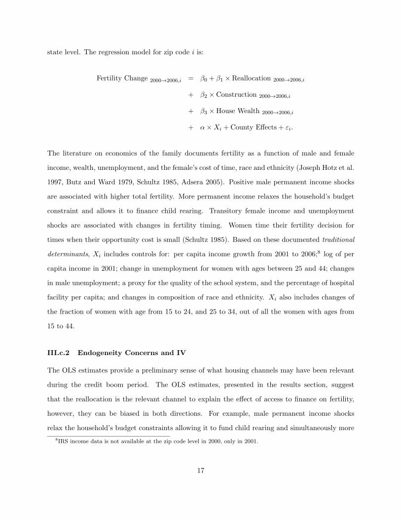
state level. The regression model for zip code i is:

Fertility Change 2000→2006,i = β0 + β1 × Reallocation 2000→2006,i

+ β2 × Construction 2000→2006,i

+ β3 × House Wealth 2000→2006,i

+ α×Xi + County Effects + εi.

The literature on economics of the family documents fertility as a function of male and female

income, wealth, unemployment, and the female’s cost of time, race and ethnicity (Joseph Hotz et al.

1997, Butz and Ward 1979, Schultz 1985, Adsera 2005). Positive male permanent income shocks

are associated with higher total fertility. More permanent income relaxes the household’s budget

constraint and allows it to finance child rearing. Transitory female income and unemployment

shocks are associated with changes in fertility timing. Women time their fertility decision for

times when their opportunity cost is small (Schultz 1985). Based on these documented traditional

determinants, Xi includes controls for: per capita income growth from 2001 to 2006;8 log of per

capita income in 2001; change in unemployment for women with ages between 25 and 44; changes

in male unemployment; a proxy for the quality of the school system, and the percentage of hospital

facility per capita; and changes in composition of race and ethnicity. Xi also includes changes of

the fraction of women with age from 15 to 24, and 25 to 34, out of all the women with ages from

15 to 44.

III.c.2 Endogeneity Concerns and IV

The OLS estimates provide a preliminary sense of what housing channels may have been relevant

during the credit boom period. The OLS estimates, presented in the results section, suggest

that the reallocation is the relevant channel to explain the effect of access to finance on fertility,

however, they can be biased in both directions. For example, male permanent income shocks

relax the household’s budget constraints allowing it to fund child rearing and simultaneously more

8IRS income data is not available at the zip code level in 2000, only in 2001.

17

easily obtain a mortgage loan. In this case, if such a shocks are not appropriately controlled for,

OLS estimates of the impact of reallocation on fertility is biased upwards. On the other hand, a

shock to the female’s level of education or potential labor income creates a negative bias since the

female’s opportunity cost of child rearing increases, but at the same time the chance of qualifying

for a mortgage loan increase. To identify the effect of access to finance on the household’s fertility

decision, I need an instrumental variable that correlates with fertility through the channel of interest

- reallocation - and not through any other unobservable factor that drives fertility.

The empirical design is defined by four features. First, I assume that, between 2000 and 2006,

the whole U.S. economy experienced an outward shift on supply of credit led by relaxation of credit

standards (Mian and Sufi 2009; Keys, Mukherjee, Seru, and Vig 2010, Adelino, Schoar, and Severino

2012, Di Maggio and Kermani 2014). Second, to control for geographical differences between cities,

especially differences in labor and housing markets that could confound the identification, I include

county effects in all estimations, hence only the zip code level variation within-county is used for

identification. Third, I use zip code level variation in the fraction of homeowners who are older

than 65 and live alone in 2000 as an instrument, henceforth old homeowners, to generate plausible

exogenous variation in the supply of houses that could easily be subject to reallocation. Old

Homeowners is defined as:

old homeowners =#Homeowners Older than 65 years old and Living Alone 2000

#Households 2000.

Fourth, I control for the fraction of population in the county who is older than 65 in 2000. This

way, the empirical exercise consists in comparing the changes from 2000 to 2006 in two zip codes in

the same county, with the same fraction of old population, but different levels of old homeowners

who live alone. In a more conservative specification, I also include the fraction of homeowners who

live alone and are older than 75. In this conservative specification, I aim to control for the natural

reallocation that happens in the economy regardless of the expansion of credit supply, and thus

provide a conservative estimation of the effect of access to credit on fertility outcomes.

The source of variation of the instrument relies on the underlying motives that old households

have to exit their houses. During the housing boom, old homeowners exited their houses because

18

they could monetize their home values, could not afford to pay increasing property taxes, or suf-

fered from age-related health adversities such as death or disability. I claim that the exit due to

monetization and increasing property taxes is driven by the global increase in house prices that

was caused by the credit supply shock. Some old homeowners have a reservation price for their

houses that credit constrained households can only pay when credit standards are loosened. Other

old homeowners sell their houses and move out of their neighborhood when, due to increases in

property assessments induced by the credit boom, property taxes rise to unaffordable levels relative

to their income. The exit due to age-related health adversities is independent of the credit supply

shock. Between 2000 and 2006 and within-county, the change in mortgage origination per capita

is much larger in zip codes with high fraction of old homeowners relative to zip codes with low

fraction of old homeowners, implying that the rank condition is met. Moreover, the increase in

homeownership for young households (age<44) and decrease in homeownership for old households

(age>65) is also larger in zip codes with high fraction of old homeowners.

The instrument then isolates mortgage origination associated with reallocation of young house-

holds with old homeowners who live alone. By projecting the change in mortgage origination per

capita on the instrument defined as old homeowners, the first stage will pick up mortgage origina-

tion that is associated with reallocation.9 The exclusion restriction is guaranteed by two conditions.

First, young households move into to houses of old homeowners who live alone because of the easier

access to credit, and not due to self-selection motives associated with other determinants of fertil-

ity, such as increases in unobservable permanent income. Second, the within-county zip code level

variation of old homeowners who live alone in 2000 is not confounded by an omitted variable, such

as unobservable school quality, which would consistently predict higher fertility outcomes in these

zip codes regardless of an easier access to credit. To ensure that the exclusion restriction is met, I

introduce a more conservative empirical design that controls for the level of old homeowners who

live alone and are older that 75. Since the average life expectancy in the U.S. is 76 years for males

and 81 years for females, shifting the age limit to 75 years old, increases the weight on the exit due

to health-related reasons, a ‘natural’ reallocation mechanism. Hence, by attempting to control for

9I assume that within-county houses are on average larger than apartments and thus suitable for young householdsto form and expand their families. I present anecdotal evidence in section III.a that supports this assumption.

19

‘natural’ reallocation, the effect captured by the variation of homeowners who live alone and are

older than 65 will not be contaminated by self-selection motives.

One may still be concerned with the exclusion restriction of the aforementioned identification,

particularly because unobservable income innovations could drive housing demand of young and

credit constrained households and consequently lead them to purchase homes of old homeowners,

regardless of the credit supply shock.

If the effect of access to credit on fertility is driven by other factors that are not associated to the

credit supply shock, it is plausible that the same effect will also be present before the expansion of

mortgage credit, in particular from 1995 to 2000, a period when the US economy experienced high

income growth and house price growth. One can conduit two tests. First, during the period from

1995 to 2000, does per capita mortgage origination changes faster in zip codes with old homeowners

who live alone? Second, during the period from 1995 to 2000, does per fertility changes faster in zip

codes with old homeowners who live alone? If the impact of the instrument on fertility is zero when

the credit induced reallocation channel is turned off, it will lend more confidence to the exclusion

restriction. The answer to the both questions is no.There is no relative difference in mortgage

origination from 1995 and 2000 in zip codes with old homeowners who live alone. There is no

difference in fertility changes during this period in zip codes with old homeowners who live alone.

During a period when the first stage fails, the instrument has no effect on the outcome variable.

Lastly, although the empirical design may be valid, it does not guarantee external validity of

the results. Young credit constrained households can achieve space through reallocation by moving

into to a vacant house, a house where the previous household was dissolved, a house where the

current household upgrades to a larger house, or a house where the current household downsizes to

a smaller house. Under these different options for reallocation, one should be concerned whether the

treatment effect of reallocation on fertility produced by the variation of old homeowners is the same

as the average treatment effect of all types of space increase on fertility. The causal mechanism

of reallocation is that access to space causes family expansion. Therefore, it seems plausible to

assume that as long as young households access more space they will expand their families, despite

who the previous homeowners were or the conditions that led the previous household to leave the

20

house. Under this assumption, that space is a key variable, I assume that the local treatment effect

estimated in the empirical design on this paper is equal to the average treatment effect of access to

credit on fertility outcomes.

Table 10 reports the OLS regression coefficients of old homeowners on the change in home-

ownership for different age groups, after controlling for county effects. Table 10 shows that the

instrument captures precisely the variation of interest. In zip codes with high fraction of old home-

owners, the homeownership increased for households whose head age is between 25 and 34 as well

as between 35 and 44. The correlation coefficient is equal to 0.34 and 0.46, respectively, and statis-

tically significant. On the other hand, the correlation coefficient on the change in homeownership

for households whose head age is between 65 and 74 is -0.35, and above 75 is -0.49. The regression

coefficient on the change in homeownership for households whose head age is between 44 and 65

is almost zero and insignificant. These regression coefficients show that, from 2000 to 2006, in zip

codes with high fraction of old homeowners there was a reallocation of the housing stock whereby

old households sold their houses to younger households.

To implement the empirical strategy discussed above, I use a two stage least squares estimation

(2SLS). In the first stage, I estimate:

Reallocation Measure2000→2006,i = θ0 + θ1 ×[

#Homeowners, age>65 and Living Alone

#Households

]2000,i

+ θ2 × Construction Measure 2000→2006,i

+ θ3 × House Price Measure 2000→2006,i

+ θ4 × % Pop Age>65 2000→2006,i + Θ ×Xi + County Effects + ηi,

and in the second stage, I estimate:

Fertility Change 2000→2006,i = β0 + β1 × Reallocation Measure 2000→2006,i

+ β2 × Construction Measure 2000→2006,i

+ β3 × House Price Measure 2000→2006,i

+ β4 × % Pop Age>65 2000→2006,i + α×Xi + County Effects + εi.

21

Vector Xi includes controls for: per capita income growth from 2001 to 2006;10 log of per capita

income in 2001; change in unemployment for women with ages between 25 and 44; changes in

male unemployment; a proxy for the quality of the school system, and the percentage of hospital

facility per capita; and changes in composition of race and ethnicity. Xi also includes changes of

the fraction of women with age from 15 to 24, and 25 to 34, out of all the women with ages from

15 to 44.

As discussed above, a more conservative specification includes as control:

[#Homeowners, age>75 and Living Alone

#Households

]2000,i

,

to measure reallocation that naturally happens in the economy regardless of the existence of a

credit supply shock.

IV RESULTS

IV.a OLS: Zipcode Level

Traditional Determinants

Previous literature has documented various determinants of fertility, namely male and female

income, wealth, unemployment, and the female’s cost of time, race and ethnicity (Joseph Hotz,

Klerman, and Willis 1997, Butz and Ward 1979, Schultz 1985, Adsera 2005). Since I can mea-

sure most of these determinants, I can estimate them, and then compare the estimated signs and

magnitudes to the ones previously found in the literature. Table 2 reports that the change in

male unemployment correlates negatively with the change in fertility from 2000 to 2006 and is

statistically significant. On the other hand, female unemployment is positively correlated with the

fertility change and very significant. Male unemployment reduces household’s fertility because of

the large negative income shock and uncertainty associated with the loss of employment (Butz

and Ward 1979). Given male unemployment, female unemployment is commonly associated with

10IRS income data is not available at the zip code level in 2000, only in 2001.

22

timing whereby women choose to have children when their opportunity cost of child rearing is low

(Schultz 1985). The signs of the two unemployment coefficients match the ones found previously

in the fertility literature. Although not statistically significant, the level of income, measured by

IRS data, is negatively correlated with fertility changes. Lower income households are more likely

to have more children (Galor and Weil 2000); for example, teenagers in low income families tend

to have higher fertility rates than teenagers in high income families. The per capita income growth

effect, measured with the IRS data, on fertility is positive, and statistically significant than zero

with a p-value of 0.02. When households experience positive income innovations they can afford

child rearing more easily. The effect of number of hospitals per capita, a proxy for the quantity

of health care facilities in the zip code, on fertility change from 2000 to 2006 is statistically zero.

During the housing boom, there is no statistical difference in fertility changes with different school

quality, as measured by the schooling score in 2004. Table 3 reports the coefficients on the age and

demographic variables of the same regression. Consistent with the literature on fertility (Parrado

and Morgan 2008), zip codes where the fraction of Hispanics increases experience an increase in

fertility. Likewise, if the zip code experiences an increase in the fraction of blacks it also experiences

an increase in fertility. Finally, zip codes that experience larger changes in the relative number of

women with ages between 25 and 24 experience higher increases in fertility between 2000 and 2006.

The effect is the opposite if the zip code experience an increase in women with ages between 15

and 24.

IV.b Discussion of the Housing Channels

I examine three housing channels that can link the expansion of credit and fertility decisions:

wealth gains from house price increases, new construction, and more efficient reallocation of the

existing housing stock among households. The goal is to isolate the space channel associated with

reallocation as a new causal channel of access to credit on fertility. To this end, I first estimate,

in an ordinary least squares framework, the three housing channels controlling for the traditional

determinants of fertility. Then, using an instrumental variable approach, I isolate the mortgage

origination associated with the reallocation channel and address endogeneity concerns that arise

23

from the OLS estimation. I present the results of the IV estimation in the next section, while in this

one, I discuss the OLS estimation based on the results reported in Table 2. The OLS estimation

allows the following three inferences:

First, I find that the house wealth channel had no effect on fertility outcomes between 2000 and

2006. The results suggest that given an increase in house prices, the negative effect on fertility from

renters cancels out the positive effect from homeowners. Dettling and Kearney (2011) use MSA

level house price variation to study the house wealth effect on fertility decisions from 1996 to 2006.

They find that a $10,000 increase in house prices is associated with a 5% increase in births among

homeowners and a 2.4% decrease among non-owners. At the mean of U.S. homeownership rate

the net effect is 0.8%. One possible explanation for the difference between my results and theirs

relies on the heterogeneity of house price growth across metropolitan areas from 1996 to 2006, since

in contrast with the early 2000s, house price growth from 1996 to 2000 happened mainly in high

income growth areas (Glaeser, Gottlieb, and Tobio 2012; Ferreira and Gyourko 2011). Dettling and

Kearney (2011)’s results could be drawing from the beginning of their sample, while mine draw

from the second part of the time period they analyze. Table 12 provides supporting evidence for

this hypothesis. The correlation between house price growth between 1996 and 2000 and fertility

change from 1995 and 2000 is 0.338 and statistically different than zero at 1% level, while the

correlation between house price growth from 2000 to 2006 and fertility change during the same

period is 0.024 with a p-value of 0.31.

The second inference is that, when measured by zip code growth in the number of house units,

the space effect due to new construction channel is negative. A one standard deviation increase in

growth in number of bedrooms (0.26) leads to a 1.8% decline in fertility from 2000 to 2006, which

is 7% of a standard deviation of fertility change. The negative sign suggests that new construction

is associated with older households who have passed the fertility age. Moreover, the negative sign

corroborates an equilibrium where households move up, meaning older households move up to

new houses and young households move into existing houses. In Table 11, I present evidence that

corroborates this hypothesis. Zip codes that experienced high growth in construction experienced

positive changes in homeownership for households older than 60. On the other hand, the new

24

construction variation does not explain the change in homeownership for housesholds younger than

44. Under this view, the new construction channel is consistent with the reallocation channel.

Third, reallocation, as measured by the change in per capita mortgages originated and sold,

correlates positively with the change in fertility. The beta coefficient without controls is 0.155

and statistically different than zero. After accounting for other traditional determinants and the

other housing channels, the OLS beta coefficient decreases to 0.140. It barely changes. Table 4

shows that the beta coefficient is 0.148 if we measure reallocation with the change in mortgage loans

originated and sold minus mortgages originated but not sold. On the other hand, if we consider total

mortgage origination as a measure of credit induced reallocation, the coefficient is 0.124. In both

cases the OLS coefficients are statistically significant than zero. This evidence is consistent with

the expansion of mortgage credit was fueled by the ability to originate and distribute that lender’s

experienced during the beginning of the 2000s. Although the OLS coefficients seem very stable with

the addition of a long list of controls, the OLS coefficient can still be biased in either direction.

Furthermore, per capita mortgage change is a noisy proxy for reallocation, there are many cases

in which mortgages are originated for borrowers who, for example, have past the fertility period,

or are not even a family. In the following section, to address this potential identification issues, I

instrument the variation of mortgage origination with the fraction of homeowners who live alone

and are older than 65 (old-homeowners), as discussed in the section III.c.2.

IV.c Instrumental Variable: Old Homeowners

To address the identification issues discussed above, I introduce in this section a novel instru-

ment that uses the fraction of homeowners who live alone and are older than 65, old homeowners, to

generate variation in credit induced reallocation that is potentially uncorrelated with other unob-

servable determinants of fertility rates. Two important additional features of the empirical design

is to control for the fraction of the population that is older than 65, and to control for the fraction of

the homeowners who live alone and are older than 75, 75-homeowners. The first feature guarantees

that the instrument is not picking variation associated with young versus old neighborhoods, the

second additional feature provides a lower bound for the credit induced reallocation by separating

25

off the natural reallocation that occurs in the economy in the absence of a credit supply shock.

Table 5 reports the first-stage and the IV estimates of the effect of access to credit on fertility

outcomes. In the first-stage, the estimated beta coefficient on old homeowners is 0.127 with a t-

statistic of 5.15, implying a F-statistic of 15.45.11 The first stage reinforces the importance of credit

induced reallocation during the housing boom. One standard deviation change in the fraction of

homeowners who live alone and are older than 65 leads to 1 extra mortgage originated and sold per

1000 people in the zip code. Table 5 provides four different IV specifications. The first in column

(4) only controls for the fraction of the population that is older than 65, and the fraction of the

homeowners who live alone and are older than 75. The IV beta coefficient is 0.191 and statistically

different than zero at 1% level. The second empirical specification includes all the controls described

above. The IV beta coefficient in this case is 0.181 and statistically different than zero at 1% level.

The stability of the IV coefficient across these two specifications reflects the orthogonality of the

instrument with respect to observable determinants of fertility, and reinforces the assumption that

the instrument is exogenous to unobservable determinants of fertility. Column (6) and (7) repeat the

same IV procedure, but exclude the control 75-homeowners. This specification provides an upper

bound for the credit induced reallocation. It might be the case the reallocation associated with the

homeowners older than 75 is associated with the credit supply shock. However, it might be the

case that the reallocation measured with homeowners older than 65 is mainly natural reallocation

that occurs in the economy in the absence of a credit supply shock. The first two specifications

already show that the majority of the reallocation effect is coming from homeowners who are with

ages between 65 and 75. Column (6) and (7) show the upper bound for the effect credit induce

reallocation on fertility outcomes. The IV beta is equal to 0.330 and statistically significant than

zero.

Table 6 and 7 replicate Table 5, but using different measures of reallocation, as discussed in

section III.b.3. Table 6 uses as reallocation measure the total mortgage origination, while Table 7

computes reallocation by subtracting mortgages originated and kept in the lender’s balance sheets

from mortgages originated and sold. The results are unchanged. The beta on Old Homeowners in

11According to Staiger and Stock (1997), who formalized the definition of weak instruments, since the F-statisticexceeds 10, the instrument is considered strong.

26

the first stage of Table 6 has higher sensitivity to the addition of controls, a reflection that Total

Origination is a noisy measure of reallocation relative to the other two measures. In opposition,

the beta on Old Homeowners in the first stage of Table 7 is very stable after adding a long list of

controls, and is higher than the counterpart in Table 6. The IV betas vary within the same range

than the ones presented in Table 5.

IV.d Economic Magnitude

To estimate the magnitude of the effect of the access to credit through the reallocation channel,

I use county level data because the zip code dataset only covers 25% of the US population. I start

by sorting counties by change in the per capita mortgage origination from 2000 to 2006. I use the

whole sample of counties where I have data on births and loans from HMDA, that is 2091 counties

that cover approximately 93% of the U.S. population. I create 20 equal sized bins, and using the

estimated sensitivities from the IV regression, I estimate the change in fertility for each bin from

2000 to 2006. According to the estimates presented in Tables 5, 6, and 7, I use a beta of 0.20 as

lower bound, and 0.30 as upper bound. Then, using the change in fertility and number of women

of child bearing age in each bin, I compute the number of births in 2006 in each bin due to the

reallocation channel. Finally, I assume the bottom bin to be the ‘control’ bin and the others to be

the ‘treatment’ bins. The estimate of births in 2006 is then equal to the sum of ‘treatment’ bins

minus ‘control’ bin. Using this methodology and relying on the assumption that the bottom bin

is a fair ‘control’ group, the estimated upper bound number of births is equal to 136,000 in 2006,

while the lower bound is 90,000. If I assume that the growth in fertility is linear from 2001 to

2006, as Figure 1 suggests, then in 2001 I estimate the upper bound number of births to be 22,800,

and the lower bound 15,000. The sum of all the reallocation-related births from 2001 to 2006 falls

between 317,000 and 478,000. About 2% to 3% of the children that were born in 2006 were due to

the housing boom.

IV.e Life-time versus Life-cycle Effect

Such a large increase in the number of births begs the question on how much of this increase

was a life-time change—a permanent change in the number of births—or a life-cycle change—a

27

change in the timing when households choose to have children. Both cases are important, but have

different implications in the economy. To understand the nature of the change in the number of

births, I study the fertility changes after the housing boom, from 2006 to 2010. If the increase in

fertility during the housing boom was a life-time change, no relative difference should exist between

high and low old homeowners zip codes after the housing boom. On the other hand, if the change

in fertility during the housing boom was a life-cycle change, then a correction in fertility outcomes

should be observable after the housing boom. Table 9 reports the regression coefficients of a similar

empirical design as discussed in III.c.2, except that the dependent variable is the change in fertility

from 2006 to 2010. The OLS beta coefficients are not statistically different than zero. However,

they can be largely biased because many shocks during the financial crisis that can explain the

change in fertility are correlated with the distribution of the credit supply shock. Using the same

instrument than above, Table 9 also reports the IV estimated betas. The IV betas on the other

hand are negative, large and statistically significant. One standard deviation change in the per

capita mortgages originated and sold leads a decrease in approximately 5.8 units in fertility from

2006 to 2010. From the analysis between 2000 and 2006, the same increase in per capita mortgages

originated and sold leads to an increase in from 2.60 to 4.3 units in fertility. The drop from 2006 to

2010 is larger than then increase form 2000 to 2006, implying that the increase in fertility during

the housing boom was potentially undone during the financial crisis. Although the empirical design

is not ideal because it does not control for several other channels that might have impacted fertility

outcomes during the financial crisis, the current results point in the direction of a life-cycle change

rather than a life-time change. Another potential issue with the results from 2006 to 2010, is the

amount of migration that resulted from foreclosures. These effect is more likely to be strong in zip

codes that experienced large increase in mortgage origination during the housing boom. Further

research on fertility behavior during the financial crisis is needed.

28

V Concluding Remarks

This paper introduces a new welfare effect of access to finance whereby access to credit can offer

welfare improvements, namely in fertility outcomes. I conduct within-county analysis with zip code

level data to document that changes in mortgage origination are strongly associated with changes

in fertility rates beyond traditional fertility determinants such as income and unemployment. I

examine three housing channels that could explain this correlation: wealth gains from house price

increases, new construction, and more efficient reallocation of the existing housing stock among

households. I claim that after controlling for the house wealth and construction channel, mortgage

origination measures the reallocation channel. The reallocation allows young households to move

to larger homes or achieve homeownership earlier in their life-cycle, while older households can

downsize their housing consumption. I exploit zip code level variation in fraction of homeowners

older than 65 and living alone to causally identify the reallocation channel. During the housing

boom, old homeowners exited their houses because they could monetize their home value, could

not afford to pay increasing property taxes, or suffered from age-related health adversities such

as death or disability. I claim that the exit due to monetization and property taxes is driven by

the credit supply shock. Some old homeowners have a reservation price for their house that credit

constrained households can only pay when credit standards are loosened. Other old homeowners

sell their houses and move out of the neighborhood because property taxes raise to unaffordable

levels relative to their income, when property assessments increase induced by the credit boom.

The exit due to age-related health adversities is purely exogenous. The variation generated by the

instrument allows me estimate the causal effect of access to finance on fertility decisions through the

reallocation channel. The IV estimates show that one standard deviation increase in reallocation

leads to a 4.6% to 7% increase in fertility from 2000 to 2006, which represents 20% to 30% of the

standard deviation of fertility change.

Beyond the direct impact on utility and the impact on expenditures, fertility decisions produce

significant changes at the aggregate level by affecting population growth and economic growth

(Barro and Becker 1989 and Becker et al. 1990). Therefore, if the expansion of credit affected the

fertility rate of U.S. households, it is relevant to estimate the magnitude of the aggregate effect. I

29

estimate that approximately 330,000 to 480,000 babies were born between 2000 and 2006 due to

the reallocation channel.

How much of this increase was a life-time change or a life-cycle change? I show that, between

2006 and 2010, zip codes that experienced high levels of credit induced reallocation were more

likely to experience large drops in fertility outcomes. The drop is larger is size than the increase,

implying that the increase in fertility during the housing boom was undone during the financial

crisis. Although the empirical design is not ideal because it does not control for several other

channels that might have impacted fertility outcomes during the financial crisis, the current results

point in the direction of a life-cycle change rather than a life-time change. This paper not only

contributes to the literature on the welfare effects associated to the access to finance, but also

documents a determinant of fertility that was not well-identified.

References

Adelino, M., A. Schoar, and F. Severino (2012, February). Credit supply and house prices: Evi-

dence from mortgage market segmentation. Working Paper 17832, National Bureau of Economic

Research.

Adsera, A. (2005). Vanishing children: From high unemployment to low fertility in developed

countries. The American Economic Review 95 (2), pp. 189–193.

Angrist, J., V. Lavy, and A. Schlosser (2010). Multiple experiments for the causal link between the

quantity and quality of children. Journal of Labor Economics 28 (4), pp. 773–824.

Barro, R. J. and G. S. Becker (1989). Fertility choice in a model of economic growth. Economet-

rica 57 (2), pp. 481–501.

Becker, G. S. (1960). An economic analysis of fertility. In Demographic and Economic Change in

Developed Countries, pp. 209–240. Columbia University Press.

Becker, G. S. (1965). A theory of the allocation of time. The Economic Journal 75 (299), pp.

493–517.

30

Becker, G. S. and H. G. Lewis (1973). On the interaction between the quantity and quality of

children. The Journal of Political Economy 81 (2), S279–S288.

Becker, G. S., K. M. Murphy, and R. Tamura (1990). Human capital, fertility, and economic

growth. Journal of Political Economy 98 (5), S12–37.

Butz, W. P. and M. P. Ward (1979). The emergence of countercyclical u.s. fertility. The American

Economic Review 69 (3), pp. 318–328.

Charles, K. K., E. Hurst, and M. J. Notowidigdo (2013, April). Manufacturing decline, housing

booms, and non-employment. (18949).

Dettling, L. J. and M. S. Kearney (2011, October). House prices and birth rates: The impact of

the real estate market on the decision to have a baby. Working Paper 17485, National Bureau

of Economic Research.

Di Maggio, M. and A. Kermani (2014). Credit-induced boom and bust. Available at SSRN 2463516 .

Ermisch, J. F. (1989). Purchased child care, optimal family size and mother’s employment: Theory

and econometric analysis. Journal of Population Economics 2 (2), pp. 79–102.

Felson, M. and M. Solaun (1975). The fertility-inhibiting effect of crowded apartment living in a

tight housing market. American Journal of Sociology 80 (6), pp. 1410–1427.

Ferreira, F. and J. Gyourko (2011, August). Anatomy of the beginning of the housing boom: U.s.

neighborhoods and metropolitan areas, 1993-2009. Working Paper 17374, National Bureau of

Economic Research.

Galor, O. and D. N. Weil (1996). The gender gap, fertility, and growth. The American Economic

Review 86 (3), pp. 374–387.

Galor, O. and D. N. Weil (2000). Population, technology, and growth: From malthusian stagnation

to the demographic transition and beyond. American economic review , 806–828.

Gertler, P., D. I. Levine, and E. Moretti (2009). Do microfinance programs help families insure

consumption against illness? Health Economics 18 (3), 257–273.

Glaeser, E. L., J. D. Gottlieb, and K. Tobio (2012). Housing booms and city centers. American

Economic Review 102 (3), 127–33.

Greenwood, R. and D. Scharfstein (2013). The growth of finance. Journal of Economic Perspec-

tives 27 (2), 3–28.

Guerrieri, V., D. Hartley, and E. Hurst (2013). Endogenous gentrification and housing price dy-

namics. Journal of Public Economics 100 (0), 45 – 60.

31

Jappelli, T. and L. Pistaferri (2011). Financial integration and consumption smoothing. The

Economic Journal 121 (553), 678–706.

Joseph Hotz, V., J. A. Klerman, and R. J. Willis (1997). The economics of fertility in developed

countries. Handbook of population and family economics 1, 275–347.

Kaplan, S. N. and J. Rauh (2010). Wall street and main street: What contributes to the rise in

the highest incomes? Review of Financial Studies 23 (3), 1004–1050.

Karlan, D. and J. Zinman (2010). Expanding credit access: Using randomized supply decisions to

estimate the impacts. Review of Financial Studies 23 (1), 433–464.

Keys, B. J., T. Mukherjee, A. Seru, and V. Vig (2010). Did securitization lead to lax screening?

evidence from subprime loans. The Quarterly Journal of Economics 125 (1), 307–362.

Kohler, H.-P., J. R. Behrman, and A. Skytthe (2005). Partner + children = happiness? the effects

of partnerships and fertility on well-being. Population and Development Review 31 (3), 407–445.

Kulu, H. and A. Vikat (2007). Fertility differences by housing type: The effect of housing conditions

or of selective moves? Demographic Research S6 (26), 775–802.

Levine, R. and Y. Rubinstein (2013, August). Liberty for more: Finance and educational oppor-

tunities. Working Paper 19380, National Bureau of Economic Research.

Malthus, T. R. (1798). An essay on the principle of population, Volume 1. Norton, New York.

Margolis, R. and M. Myrskyla (2011). A global perspective on happiness and fertility. Population

and Development Review 37 (1), 29–56.

Melzer, B. T. (2011). The real costs of credit access: Evidence from the payday lending market.

The Quarterly Journal of Economics 126 (1), 517–555.

Mian, A. and A. Sufi (2009). The consequences of mortgage credit expansion: Evidence from the

u.s. mortgage default crisis. The Quarterly Journal of Economics 124 (4), 1449–1496.

Mian, A. R. and A. Sufi (2012, February). What explains high unemployment? the aggregate

demand channel. (17830).

Mincer, J. (1963). Market prices, opportunity costs, and income effects. Measurement in economics,

67–82.

Morse, A. (2011). Payday lenders: Heroes or villains? Journal of Financial Economics 102 (1),

28–44.

32

Mulder, C. H. and F. C. Billari (2010). Homeownership regimes and low fertility. Housing Stud-

ies 25 (4), 527–541.

Parrado, E. and S. Morgan (2008). Intergenerational fertility among hispanic women: New evidence

of immigrant assimilation. Demography 45 (3), 651–671.

Philippon, T. and A. Reshef (2012). Wages and human capital in the u.s. finance industry: 1909-

2006. The Quarterly Journal of Economics.

Philippon, T. and A. Reshef (2013). An international look at the growth of modern finance. Journal

of Economic Perspectives 27 (2), 73–96.

Schultz, T. P. (1985). Changing world prices, women’s wages, and the fertility transition: Sweden,

1860-1910. Journal of Political Economy 93 (6), pp. 1126–1154.

Shu, P. (2013). Career choice and skill development of mit graduates: Are the best and brightest

going into finance?

Staiger, D. and J. H. Stock (1997, May). Instrumental variables regression with weak instruments.

Econometrica 65 (3), 557–586.

Strom, S. (2010). Housing and first births in sweden, 1972-2005. Housing Studies 25 (4), 509–526.

Thomson, E. and Y. Brandreth (1995). Measuring fertility demand. Demography 32 (1), 81–96.

Willis, R. J. (1973). A new approach to the economic theory of fertility behavior. Journal of

Political Economy 81 (2), pp. S14–S64.

33

Figure 1: Fertility Rate and Mortgage Origination in US from 1990 to 2010

The top panel shows the aggregate number of births (in millions) in the U.S. between 1990 and 2000. The mid panelpresents the aggregate fertility rate for women in the U.S. in the same period. Fertility rate is defined as the totalnumber of births divided by the number of women (in thousands) with ages between 15 and 44. The aggregate dataon births is from the Centers for Disease Control and Prevention (http://www.cdc.gov/nchs/births.htm). Thebottom panel shows the aggregate value in millions of dollars of originations for home purchase from HMDA between1990 to 2010.

3.9

44

.14.2

4.3

Nu

mb

er

of

birth

s (

mill

ion

s)

1990 1995 2000 2005 2010Year

64

66

68

70

72

Fe

rtili

ty R

ate

1990 1995 2000 2005 2010Year

01

23

4M

ort

ga

ge

Orig

ina

tio

n (

mill

ion

s u

sd

)

1990 1995 2000 2005 2010Year

34

Figure 2: Annual Sales of Newly Constructed and Existing Homes in US

The top panel depicts the annual number of house transactions for newly constructed and the bottom panel reportsthe annual number of house transactions for existing homes. Both levels are presented in millions. Data was collectedfrom the National Association of Realtors website.

.4.6

.81

1.2

1.4

Annual S

ale

s N

ew

Hom

es (

mill

ions)

1990 1995 2000 2005 2010Year

34

56

7A

nnual S

ale

s E

xis

ting H

om

es (

mill

ions)

1990 1995 2000 2005 2010Year

35

Figure

3:Fertilityand

MortgageOrigination

inth

eCro

ss-S

ection:County

-Level

The

pic

ture

bel

owsh

ows

the

corr

elati

on

bet

wee

nth

efe

rtilit

ych

ange

and

the

per

capit

am

ort

gage

ori

gin

ati

on

change.

Fer

tility

rate

isdefi

ned

as

the

num

ber

of

bir

ths

div

ided

by

the

num

ber

of

wom

en(i

nth

ousa

nds)

of

ages

bet

wee

n15

and

44.

Per

capit

am

ort

gage

ori

gin

ati

on

change

isdefi

ned

as

the

mort

gage

ori

gin

ati

on

for

hom

epurc

hase

div

ided

by

the

popula

tion

(in

thousa

nds)

inth

eco

unty

.E

ach

dot

repre

sents

aco

unty

and

the

size

ispro

port

ional

toth

esi

zeof

the

popula

tion

inth

eco

unty

.O

nly

counti

esw

ith

more

than

100,0

00

peo

ple

are

plo

tted

inth

egra

ph.

The

red

line

isth

efitt

edre

gre

ssio

nline.

The

left

panel

dep

icts

the

rela

tionsh

ipb

etw

een

mort

gage

ori

gin

ati

on

and

fert

ilit

yra

tes

from

1995

to2000,

the

mid

dle

panel

from

2000

to2006

and

the

right

panel

from

2007

and

2010.

−1001020

Fertility Change

−5

05

10

15

20

Per

Capita M

ort

gage O

rigin

ation C

hange

1995−

2000

−10−5051015

Fertility Change

−10

01

02

0

Per

Capita M

ort

gage O

rigin

ation C

hange

2000−

2006

−20−10010

Fertility Change

−15

−10

−5

05

Per

Capita M

ort

gage O

rigin

ation C

hange

2007−

2010

36

Figure 4: Fertility Rate in Top and Bottom Quintile of Credit Growth

This figure presents the fertility rates for two groups of counties. Counties were sorted by the change in per capitamortgage origination for home purchase. Mortgage credit origination comes from HMDA and is defined as the totalnumber of mortgage loans originated for home purchase. The blue and green lines are the averages for the top andbottom quintiles, respectively. The red dashed lines are the bounds for the 95% confidence intervals. Fertility rate isdefined as the total number of births divided by the number of women (in thousands) with ages between 15 and 44.

60

65

70

75

80

Fe

rtili

ty R

ate

1990 1995 2000 2005 2010Year

37

Figure 5: Rent Price by Apartment Size

The picture below shows the asked price per bedroom by apartment size. Apartment size is measured by the numberof bedrooms. Asked prices are estimated from 30 million craigslist adds from 2008 to 2013 for all the cities wherecraigslist is present in the US.

02,0

00

4,0

00

6,0

00

Asked R

ent P

rice (

in d

olla

rs)

1 2 3 4 5

Number of Bedrooms in the Apartment

38

Figure 6: Changes in Homeownership Rate by Age Group during the Housing Boom

In the picture below each bar represents the change in percentage points of homeownership rate by age group. Theblue bars report the changes from 2000 to 2005 and the light yellow the changes from 1990-1995. Homeownershiprate is defined as the proportion of owner households to the total number of occupied households. The estimates arebased on the Current Population Survey and Housing Vacancy Survey.

−1

01

23

Change in H

om

eow

ners

hip

Rate

18−24 25−29 30−34 35−39 40−44 45−54 55−64 65−85

Age Group

1990−1995 2000−2005

39

Table 1: Summary of Statistics

This table presents the summary of statistics of the variables used in the empirical analysis. Total Origination/Popis defined as the mortgage origination for home purchase divided by the population (in thousands) in the zip code.(Originated & Sold)/Pop is defined as the total number of mortgages originated and sold divided by the population(in thousands) in the zip code. (Originated & Non-Sold)/Pop is defined as the total number of mortgages originatedand not sold divided by the population (in thousands) in the zip code. Fertility rate is defined as the number ofbirths divided by the number of women (in thousands) with ages between 15 and 44. IRS Income growth is computedusing the adjust gross income from the IRS data. Income and Capital Gains are reported in thousands of dollars.HP is house price growth from Zillow. Female College is the fraction of women in the zip code who have at leasta bachelor’s degree. Demographics and Unemployment are from the Census and the American Community Survey(ACS). House units growth is computed using the number of house units per zip code as reported by the Censusand ACS. Old-Homeowners is the instrumental variable that measures fraction of homeowners who are older than 65years-old and live alone, while 75-Homeowners measures the fraction of homeowners who are older than 75 years-oldand live alone, both described and discussed in section III.c.2. School Score is the reading score from Global ReportCard for the school district where the zip code is located. Hospitals is the number of hospital facility from the Countyof Business Patterns.

N Mean Std 10th 50th 90th

HP Growth{00→06} 2717 1.07 0.55 0.35 1.06 1.79House Units Growth{00→06} 2717 0.13 0.26 -0.014 0.068 0.32(Originated)/Pop{00→06} 2717 0.64 9.52 -8.20 0.74 9.01

(Originated & Sold)/Pop{00→06} 2717 1.71 7.10 -4.50 1.33 7.91

(Originated & Non-Sold)/Pop{00→06} 2717 -1.07 3.16 -4.56 -0.65 1.74

Male Unemployment{00→06} 2717 0.016 0.036 -0.021 0.019 0.053

Female Unemployment{00→06} 2717 0.011 0.036 -0.026 0.014 0.047

Female Unemployment{2000} 2717 0.064 0.046 0.024 0.051 0.12

Per Capita Inc. Growth{00→06} 2717 0.22 0.17 0.075 0.19 0.40

Log Per Capita Income{2000} 2717 3.83 0.47 3.34 3.75 4.42

Fraction of Hisp.{00→06} 2717 0.029 0.041 -0.0082 0.021 0.084

Fraction of Black.{00→06} 2717 0.0034 0.033 -0.022 0.0022 0.034Fertility{2000} 2717 62.2 17.8 41.6 60.5 84.7

Fertility{2006} 2717 65.6 22.0 40.9 63.6 92.5

Fertility{2010} 2717 52.4 26.6 0 56.5 80.9

Fertility{00→06} 2717 3.34 14.4 -11.6 2.25 19.1

Fertility{06→10} 2717 -13.2 24.3 -53.0 -7.28 7.46

School Score{2004} 2717 48.7 15.2 26.9 48.1 69.7Hospitals/Pop{2000} 2717 0.017 0.044 0 0 0.059

Old-Homeowners{2000} 2717 0.018 0.010 0.0064 0.016 0.03075-Homeowners{2000} 2717 0.0088 0.0059 0.0024 0.0079 0.016% Pop w/ Age>65{2000} 2717 0.14 0.078 0.068 0.12 0.22

Population{2000} 2717 24846.9 18146.3 5077 21396 48674

40

Table 2: Mortgage Origination and Fertility During The Boom: OLS

This table reports the OLS betas of the model presented in section III.c.1 when the reallocation measure is based onthe mortgages originated and sold. (Originated & Sold)/Pop is defined as the total number of mortgages originatedand sold divided by the population (in thousands) in the zip code. Fertility rate is defined as the number of birthsdivided by the number of women (in thousands) with ages between 15 and 44. IRS Income growth is computed usingthe adjust gross income from the IRS data. Income and Capital Gains are reported in thousands of dollars. HP ishouse price growth from Zillow. Female College is the fraction of women in the zip code who have at least a bachelor’sdegree. Demographics and Unemployment are from the Census and the American Community Survey (ACS). Houseunits growth is computed using the number of house units per zip code as reported by the Census and ACS. Old-Homeowners is the instrumental variable that measures fraction of homeowners who are older than 65 years-old andlive alone, while 75-Homeowners measures the fraction of homeowners who are older than 75 years-old and live alone,both described and discussed in section III.c.2. School Score is the reading score from Global Report Card for theschool district where the zip code is located. Hospitals is the number of hospital facility from the County of BusinessPatterns. ***,**,* coefficient estimate statistically distinct from 0 at the 1%, 5% and 10% levels, respectively; p-valuesin parentheses. All regressions are weighted by the county population. This table continues in the next page.

Fertility Change from 2000 to 2006

OLS OLS OLS OLS OLS OLS

(Originate & Sold)/Pop{00→06} 0.155∗∗∗ 0.140∗∗∗ 0.140∗∗∗

(0.00) (0.00) (0.00)HP Growth{00→06} -0.017 0.030 -0.017 -0.072 -0.072

(0.77) (0.18) (0.77) (0.20) (0.21)House Units Growth{00→06} -0.055∗ -0.064 -0.055∗ -0.076∗∗ -0.083∗∗∗

(0.08) (0.14) (0.08) (0.01) (0.01)Male Unemployment{00→06} -0.031 -0.031 -0.039 -0.040∗

(0.17) (0.17) (0.11) (0.09)Female Unemployment{00→06} 0.084∗∗∗ 0.084∗∗∗ 0.084∗∗∗ 0.083∗∗∗

(0.00) (0.00) (0.00) (0.00)Female Unemployment{2000} 0.007 0.007 -0.007 -0.007

(0.82) (0.82) (0.79) (0.78)Per Capita Inc. Growth{00→06} 0.079∗∗ 0.079∗∗ 0.070∗∗ 0.071∗∗

(0.02) (0.02) (0.02) (0.02)Log Per Capita Income{2000} -0.042 -0.042 -0.037 -0.014

(0.45) (0.45) (0.48) (0.75)School Score{2004} -0.030 -0.030 -0.016 -0.019

(0.20) (0.20) (0.42) (0.25)Hospitals/Pop{2000} 0.001 0.001 0.003 0.007

(0.94) (0.94) (0.86) (0.69)75-Homeowners{2000} 0.036

(0.12)% Pop w/ Age>65{2000} -0.045

(0.25)

County Effects Yes Yes Yes Yes Yes YesAge-Demo Controls No Yes No Yes Yes Yes#Zip Codes 2717 2717 2717 2717 2717 2717R-squared 0.119 0.146 0.101 0.146 0.160 0.161

41

Table 3: Mortgage Origination and Fertility During Boom.(Continuation)

This table is the continuation from the table in the previous page. Fem(a,b) is the number of females (in thousands)in the zip code with ages between a and b. Demographics are from the Census and the American Community Survey(ACS). Fertility rate is defined as the number of births divided by the number of women with ages between 15 and44. Standard errors are robust and clustered at the state level. ***,**,* coefficient estimate statistically distinct from0 at the 1%, 5% and 10% levels, respectively; p-values in parentheses. All regressions are weighted by the countypopulation.

Fertility Change from 2000 to 2006

OLS OLS OLS OLS OLS OLS

Fraction of Hisp.{00→06} 0.200∗∗∗ 0.200∗∗∗ 0.169∗∗∗ 0.163∗∗∗

(0.00) (0.00) (0.00) (0.00)Fraction of Black.{00→06} 0.055∗∗∗ 0.055∗∗∗ 0.045∗∗ 0.053∗∗

(0.00) (0.00) (0.02) (0.01)Fem (15,24)/Fem (15,45){00→06} -0.099∗ -0.099∗ -0.094∗ -0.096∗

(0.06) (0.06) (0.08) (0.07)Fem (25,34)/Fem (15,45){00→06} 0.059∗∗∗ 0.059∗∗∗ 0.047∗∗ 0.051∗∗

(0.01) (0.01) (0.02) (0.02)

County Effects Yes Yes Yes Yes Yes YesAge-Demo Controls No Yes No Yes Yes Yes#Zip Codes 2717 2717 2717 2717 2717 2717R-squared 0.119 0.146 0.101 0.146 0.160 0.161

42

Table 4: Mortgage Origination and Fertility During The Boom: OLS

This table reports the OLS betas of the model presented in section III.c.1 when the reallocation measure is based onthe total mortgages originated and the difference between mortgages originated and sold and mortgages originated butnot sold. Total Origination/Pop is defined as the mortgage origination for home purchase divided by the population(in thousands) in the zip code. ‘Sold minus NonSold’ is the difference between the mortgages originated and soldand mortgages originated but not sold and kept in the balance sheet of the lender. Fertility rate is defined as thenumber of births divided by the number of women (in thousands) with ages between 15 and 44. IRS Income growthis computed using the adjust gross income from the IRS data. Income and Capital Gains are reported in thousandsof dollars. HP is house price growth from Zillow. Female College is the fraction of women in the zip code who haveat least a bachelor’s degree. Demographics and Unemployment are from the Census and the American CommunitySurvey (ACS). House units growth is computed using the number of house units per zip code as reported by theCensus and ACS. Old-Homeowners is the instrumental variable that measures fraction of homeowners who are olderthan 65 years-old and live alone, while 75-Homeowners measures the fraction of homeowners who are older than 75years-old and live alone, both described and discussed in section III.c.2. School Score is the reading score from GlobalReport Card for the school district where the zip code is located. Hospitals is the number of hospital facility from theCounty of Business Patterns. Standard errors are robust and clustered at the state level. ***,**,* coefficient estimatestatistically distinct from 0 at the 1%, 5% and 10% levels, respectively; p-values in parentheses. All regressions areweighted by the county population.

Fertility Change from 2000 to 2006

OLS OLS OLS OLS OLS OLS

(Sold minus Nonsold)/Pop{00→06} 0.161∗∗∗ 0.149∗∗∗ 0.148∗∗∗

(0.00) (0.00) (0.00)(Total Origination)/Pop{00→06} 0.141∗∗∗ 0.124∗∗∗ 0.124∗∗∗

(0.00) (0.00) (0.00)HP Growth{00→06} -0.068 -0.068 -0.065 -0.065

(0.22) (0.22) (0.26) (0.26)House Units Growth{00→06} -0.080∗∗∗ -0.085∗∗∗ -0.071∗∗ -0.077∗∗

(0.01) (0.00) (0.02) (0.01)Male Unemployment{00→06} -0.042∗ -0.043∗ -0.036 -0.037

(0.08) (0.07) (0.14) (0.12)Female Unemployment{00→06} 0.076∗∗∗ 0.075∗∗∗ 0.087∗∗∗ 0.086∗∗∗

(0.00) (0.00) (0.00) (0.00)Female Unemployment{2000} -0.017 -0.017 -0.000 -0.000

(0.50) (0.49) (1.00) (0.99)Per Capita Inc. Growth{00→06} 0.064∗∗ 0.064∗∗ 0.074∗∗ 0.075∗∗

(0.03) (0.02) (0.02) (0.01)Log Per Capita Income{2000} -0.063 -0.041 -0.026 -0.004

(0.25) (0.37) (0.62) (0.94)School Score{2004} -0.014 -0.016 -0.019 -0.022

(0.50) (0.34) (0.34) (0.19)Hospitals/Pop{2000} 0.004 0.008 0.002 0.006

(0.78) (0.64) (0.91) (0.74)75-Homeowners{2000} 0.038∗ 0.036

(0.09) (0.12)% Pop w/ Age>65{2000} -0.043 -0.045

(0.31) (0.24)

County Effects Yes Yes Yes Yes Yes YesAge-Demo Controls No Yes Yes No Yes Yes#Zip Codes 2717 2717 2717 2717 2717 2717R-squared 0.120 0.163 0.165 0.115 0.156 0.158

43

Table 5: Mortgage Origination and Fertility During The Boom: IV

This table reports the first stage and the IV betas of the model presented in section III.c.2 when the reallocationmeasure is based on the mortgages originated and sold. (Originated & Sold)/Pop is defined as the total number ofmortgages originated and sold divided by the population (in thousands) in the zip code. Fertility rate is defined asthe number of births divided by the number of women (in thousands) with ages between 15 and 44. IRS Incomegrowth is computed using the adjust gross income from the IRS data. Income and Capital Gains are reported inthousands of dollars. HP is house price growth from Zillow. Female College is the fraction of women in the zip codewho have at least a bachelor’s degree. Demographics and Unemployment are from the Census and the AmericanCommunity Survey (ACS). House units growth is computed using the number of house units per zip code as reportedby the Census and ACS. Old-Homeowners is the instrumental variable that measures fraction of homeowners whoare older than 65 years-old and live alone, while 75-Homeowners measures the fraction of homeowners who are olderthan 75 years-old and live alone, both described and discussed in section III.c.2. School Score is the reading scorefrom Global Report Card for the school district where the zip code is located. Hospitals is the number of hospitalfacility from the County of Business Patterns. Standard errors are robust and clustered at the state level. ***,**,*coefficient estimate statistically distinct from 0 at the 1%, 5% and 10% levels, respectively; p-values in parentheses.All regressions are weighted by the county population.

(Originated & Sold)/Pop{00→06} Change in Fertility 00-06

OLS OLS OLS IV IV IV IV

(Originated & Sold)/Pop{00→06} 0.191∗∗∗ 0.181∗∗ 0.324∗∗∗ 0.330∗∗∗

(0.00) (0.01) (0.00) (0.00)Old-Homeowners{2000} 0.186∗∗∗ 0.173∗∗∗ 0.127∗∗∗

(0.00) (0.00) (0.00)% Pop w/ Age>65{2000} -0.092∗∗∗ 0.072 -0.001 -0.048 0.021 -0.048

(0.00) (0.20) (0.99) (0.14) (0.64) (0.12)75-Homeowners{2000} 0.021 -0.013 0.042∗∗ 0.034∗∗

(0.26) (0.62) (0.01) (0.05)Male Unemployment{00→06} 0.053∗ -0.042∗∗ -0.048∗∗

(0.08) (0.02) (0.02)Female Unemployment{2000} 0.116∗∗∗ -0.011 -0.029

(0.00) (0.62) (0.14)Per Capita Inc. Growth{00→06} 0.070∗∗ 0.068∗∗∗ 0.061∗∗∗

(0.01) (0.00) (0.01)Log Per Capita Income{2000} -0.035 -0.012 -0.013

(0.31) (0.74) (0.73)HP Growth{00→06} 0.396∗∗∗ -0.088 -0.149∗

(0.00) (0.16) (0.06)Female Unemployment{00→06} 0.007 0.082∗∗∗ 0.080∗∗∗

(0.74) (0.00) (0.00)House Units Growth{00→06} 0.174∗∗∗ -0.090∗∗∗ -0.116∗∗∗

(0.00) (0.00) (0.00)School Score{2004} -0.076∗∗∗ -0.015 -0.003

(0.00) (0.36) (0.86)Hospitals/Pop{2000} -0.013 0.007 0.009

(0.66) (0.61) (0.47)

County Effects Yes Yes Yes Yes Yes Yes YesAge-Demo Controls No No Yes No Yes No Yes#Zip Codes 2717 2717 2717 2717 2717 2717 2717R-squared 0.135 0.141 0.333 0.119 0.160 0.094 0.137

44

Table 6: Mortgage Origination and Fertility During The Boom: IV

This table reports the first stage and the IV beta estimates of the model presented in section III.c.2 when thereallocation measure is based on total mortgages originated. Total Origination/Pop is defined as the mortgageorigination for home purchase divided by the population (in thousands) in the zip code. Fertility rate is defined asthe number of births divided by the number of women (in thousands) with ages between 15 and 44. IRS Incomegrowth is computed using the adjust gross income from the IRS data. Income and Capital Gains are reported inthousands of dollars. HP is house price growth from Zillow. Female College is the fraction of women in the zip codewho have at least a bachelor’s degree. Demographics and Unemployment are from the Census and the AmericanCommunity Survey (ACS). House units growth is computed using the number of house units per zip code as reportedby the Census and ACS. Old-Homeowners is the instrumental variable that measures fraction of homeowners whoare older than 65 years-old and live alone, while 75-Homeowners measures the fraction of homeowners who are olderthan 75 years-old and live alone, both described and discussed in section III.c.2. School Score is the reading scorefrom Global Report Card for the school district where the zip code is located. Hospitals is the number of hospitalfacility from the County of Business Patterns. Standard errors are robust and clustered at the state level. ***,**,*coefficient estimate statistically distinct from 0 at the 1%, 5% and 10% levels, respectively; p-values in parentheses.All regressions are weighted by the county population.

(Total Origination)/Pop{00→06} Change in Fertility 00-06

OLS OLS OLS IV IV IV IV

(Total Origination)/Pop{00→06} 0.195∗∗∗ 0.214∗∗ 0.306∗∗∗ 0.363∗∗∗

(0.00) (0.01) (0.00) (0.00)Old-Homeowners{2000} 0.197∗∗∗ 0.170∗∗∗ 0.107∗∗∗

(0.00) (0.00) (0.00)% Pop w/ Age>65{2000} -0.124∗∗∗ 0.076 0.006 -0.051∗ 0.027 -0.054∗

(0.00) (0.24) (0.90) (0.09) (0.54) (0.06)75-Homeowners{2000} 0.045∗∗∗ 0.003 0.037∗∗ 0.031∗

(0.01) (0.90) (0.03) (0.07)Male Unemployment{00→06} 0.037 -0.040∗∗ -0.044∗∗

(0.15) (0.04) (0.04)Female Unemployment{2000} 0.074∗∗ -0.006 -0.018

(0.01) (0.79) (0.39)Per Capita Inc. Growth{00→06} 0.043 0.072∗∗∗ 0.068∗∗∗

(0.11) (0.00) (0.00)Log Per Capita Income{2000} -0.130∗∗ 0.009 0.023

(0.02) (0.79) (0.49)HP Growth{00→06} 0.391∗∗∗ -0.100 -0.160∗

(0.00) (0.13) (0.05)Female Unemployment{00→06} -0.020 0.088∗∗∗ 0.090∗∗∗

(0.37) (0.00) (0.00)House Units Growth{00→06} 0.155∗∗∗ -0.091∗∗∗ -0.114∗∗∗

(0.01) (0.00) (0.00)School Score{2004} -0.064∗∗∗ -0.015 -0.005

(0.00) (0.35) (0.77)Hospitals/Pop{2000} -0.007 0.007 0.007

(0.80) (0.63) (0.51)

County Effects Yes Yes Yes Yes Yes Yes YesAge-Demo Controls No No Yes No Yes No Yes#Zip Codes 2717 2717 2717 2717 2717 2717 2717R-squared 0.144 0.155 0.371 0.114 0.153 0.091 0.121

45

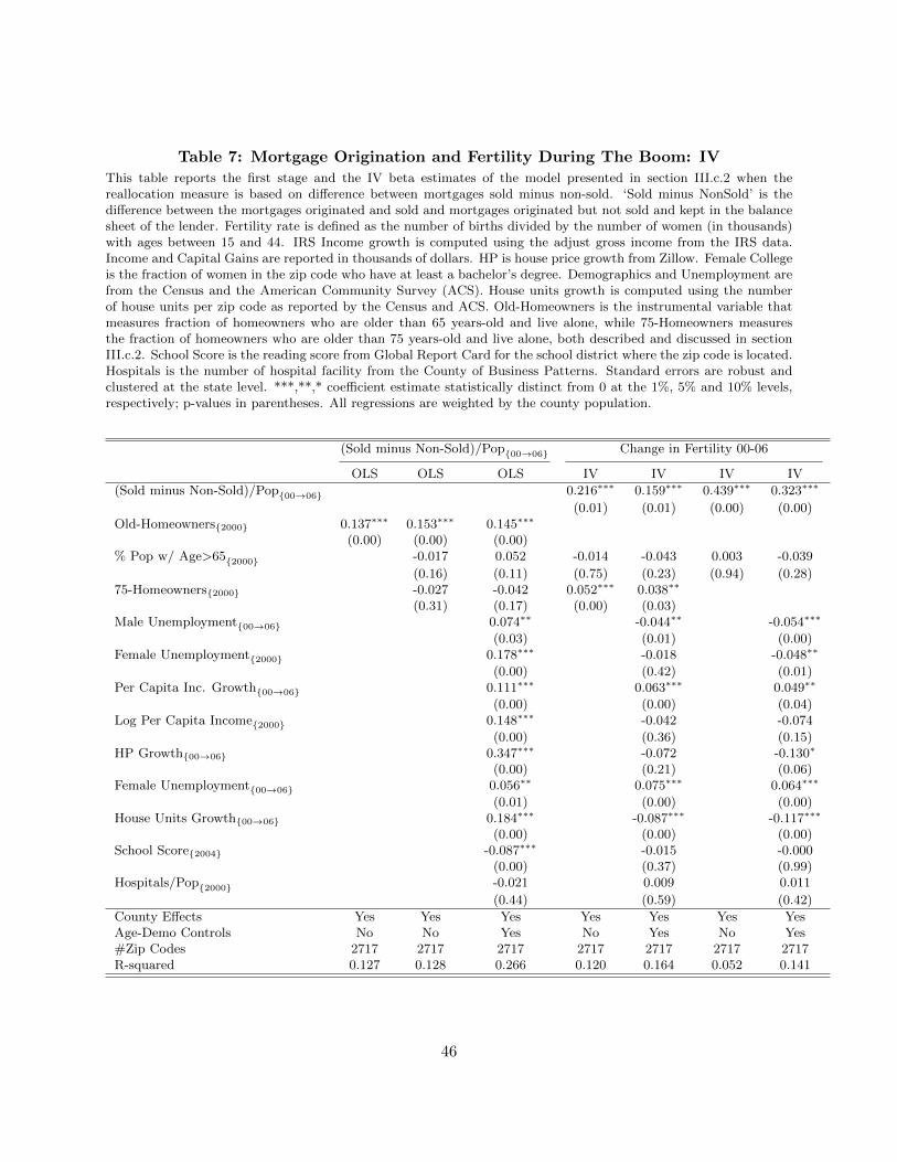
Table 7: Mortgage Origination and Fertility During The Boom: IV

This table reports the first stage and the IV beta estimates of the model presented in section III.c.2 when thereallocation measure is based on difference between mortgages sold minus non-sold. ‘Sold minus NonSold’ is thedifference between the mortgages originated and sold and mortgages originated but not sold and kept in the balancesheet of the lender. Fertility rate is defined as the number of births divided by the number of women (in thousands)with ages between 15 and 44. IRS Income growth is computed using the adjust gross income from the IRS data.Income and Capital Gains are reported in thousands of dollars. HP is house price growth from Zillow. Female Collegeis the fraction of women in the zip code who have at least a bachelor’s degree. Demographics and Unemployment arefrom the Census and the American Community Survey (ACS). House units growth is computed using the numberof house units per zip code as reported by the Census and ACS. Old-Homeowners is the instrumental variable thatmeasures fraction of homeowners who are older than 65 years-old and live alone, while 75-Homeowners measuresthe fraction of homeowners who are older than 75 years-old and live alone, both described and discussed in sectionIII.c.2. School Score is the reading score from Global Report Card for the school district where the zip code is located.Hospitals is the number of hospital facility from the County of Business Patterns. Standard errors are robust andclustered at the state level. ***,**,* coefficient estimate statistically distinct from 0 at the 1%, 5% and 10% levels,respectively; p-values in parentheses. All regressions are weighted by the county population.

(Sold minus Non-Sold)/Pop{00→06} Change in Fertility 00-06

OLS OLS OLS IV IV IV IV

(Sold minus Non-Sold)/Pop{00→06} 0.216∗∗∗ 0.159∗∗∗ 0.439∗∗∗ 0.323∗∗∗

(0.01) (0.01) (0.00) (0.00)Old-Homeowners{2000} 0.137∗∗∗ 0.153∗∗∗ 0.145∗∗∗

(0.00) (0.00) (0.00)% Pop w/ Age>65{2000} -0.017 0.052 -0.014 -0.043 0.003 -0.039

(0.16) (0.11) (0.75) (0.23) (0.94) (0.28)75-Homeowners{2000} -0.027 -0.042 0.052∗∗∗ 0.038∗∗

(0.31) (0.17) (0.00) (0.03)Male Unemployment{00→06} 0.074∗∗ -0.044∗∗ -0.054∗∗∗

(0.03) (0.01) (0.00)Female Unemployment{2000} 0.178∗∗∗ -0.018 -0.048∗∗

(0.00) (0.42) (0.01)Per Capita Inc. Growth{00→06} 0.111∗∗∗ 0.063∗∗∗ 0.049∗∗

(0.00) (0.00) (0.04)Log Per Capita Income{2000} 0.148∗∗∗ -0.042 -0.074

(0.00) (0.36) (0.15)HP Growth{00→06} 0.347∗∗∗ -0.072 -0.130∗

(0.00) (0.21) (0.06)Female Unemployment{00→06} 0.056∗∗ 0.075∗∗∗ 0.064∗∗∗

(0.01) (0.00) (0.00)House Units Growth{00→06} 0.184∗∗∗ -0.087∗∗∗ -0.117∗∗∗

(0.00) (0.00) (0.00)School Score{2004} -0.087∗∗∗ -0.015 -0.000

(0.00) (0.37) (0.99)Hospitals/Pop{2000} -0.021 0.009 0.011

(0.44) (0.59) (0.42)

County Effects Yes Yes Yes Yes Yes Yes YesAge-Demo Controls No No Yes No Yes No Yes#Zip Codes 2717 2717 2717 2717 2717 2717 2717R-squared 0.127 0.128 0.266 0.120 0.164 0.052 0.141

46

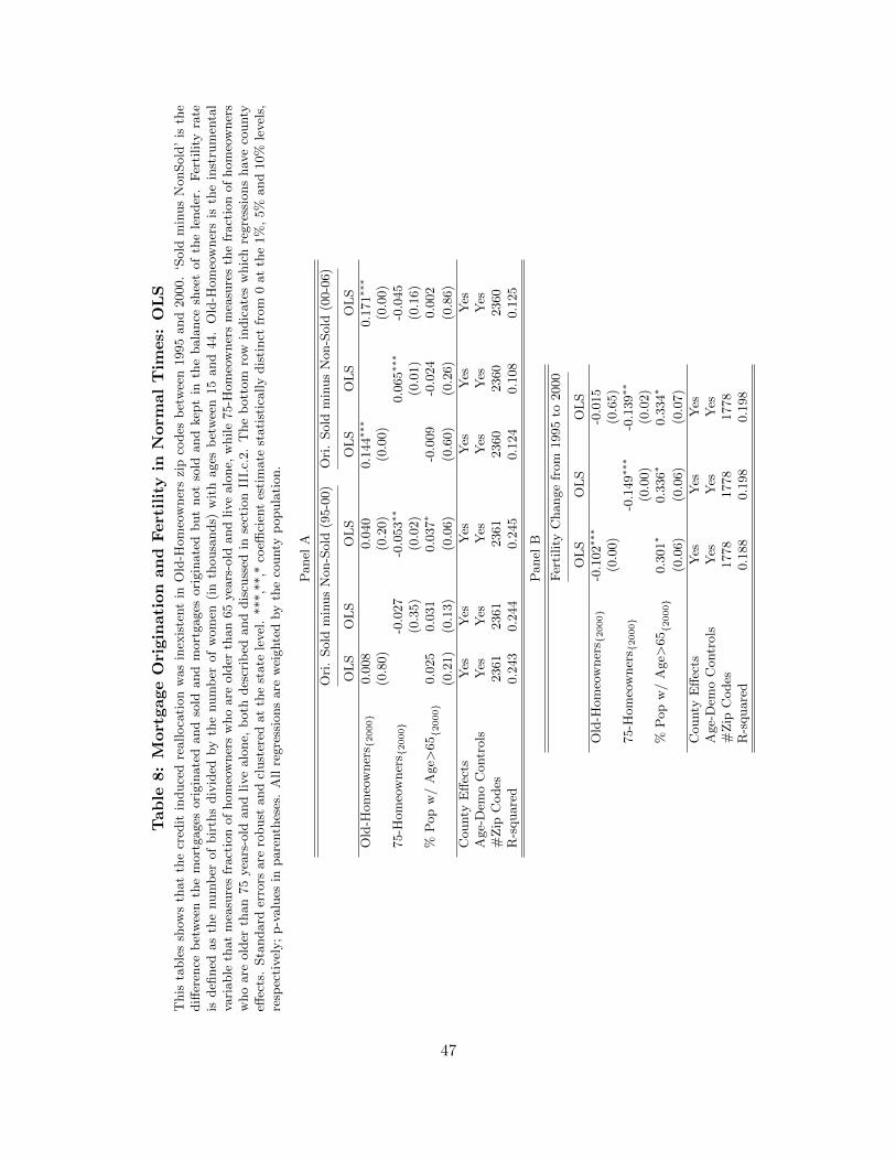
Table

8:M

ortgageOrigination

and

Fertilityin

Norm

alTim

es:

OLS

This

table

ssh

ows

that

the

cred

itin

duce

dre

alloca

tion

was

inex

iste

nt

inO

ld-H

om

eow

ner

szi

pco

des

bet

wee

n1995

and

2000.

‘Sold

min

us

NonSold

’is

the

diff

eren

ceb

etw

een

the

mort

gages

ori

gin

ate

dand

sold

and

mort

gages

ori

gin

ate

dbut

not

sold

and

kep

tin

the

bala

nce

shee

tof

the

lender

.F

erti

lity

rate

isdefi

ned

as

the

num

ber

of

bir

ths

div

ided

by

the

num

ber

of

wom

en(i

nth

ousa

nds)

wit

hages

bet

wee

n15

and

44.

Old

-Hom

eow

ner

sis

the

inst

rum

enta

lva

riable

that

mea

sure

sfr

act

ion

of

hom

eow

ner

sw

ho

are

old

erth

an

65

yea

rs-o

ldand

live

alo

ne,

while

75-H

om

eow

ner

sm

easu

res

the

fract

ion

of

hom

eow

ner

sw

ho

are

old

erth

an

75

yea

rs-o

ldand

live

alo

ne,

both

des

crib

edand

dis

cuss

edin

sect

ion

III.

c.2.

The

bott

om

row

indic

ate

sw

hic

hre

gre

ssio

ns

hav

eco

unty

effec

ts.

Sta

ndard

erro

rsare

robust

and

clust

ered

at

the

state

level

.***,*

*,*

coeffi

cien

tes

tim

ate

stati

stic

ally

dis

tinct

from

0at

the

1%

,5%

and

10%

level

s,re

spec

tivel

y;

p-v

alu

esin

pare

nth

eses

.A

llre

gre

ssio

ns

are

wei

ghte

dby

the

county

popula

tion.

Panel

A

Ori

.Sold

min

us

Non-S

old

(95-0

0)

Ori

.Sold

min

us

Non-S

old

(00-0

6)

OL

SO

LS

OL

SO

LS

OL

SO

LS

Old

-Hom

eow

ner

s {2000}

0.0

08

0.0

40

0.1

44∗∗∗

0.1

71∗∗∗

(0.8

0)

(0.2

0)

(0.0

0)

(0.0

0)

75-H

om

eow

ner

s {2000}

-0.0

27

-0.0

53∗∗

0.0

65∗∗∗

-0.0

45

(0.3

5)

(0.0

2)

(0.0

1)

(0.1

6)

%P

op

w/

Age>

65{2

000}

0.0

25

0.0

31

0.0

37∗

-0.0

09

-0.0

24

0.0

02

(0.2

1)

(0.1

3)

(0.0

6)

(0.6

0)

(0.2

6)

(0.8

6)

County

Eff

ects

Yes

Yes

Yes

Yes

Yes

Yes

Age-

Dem

oC

ontr

ols

Yes

Yes

Yes

Yes

Yes

Yes

#Z

ipC

odes

2361

2361

2361

2360

2360

2360

R-s

quare

d0.2

43

0.2

44

0.2

45

0.1

24

0.1

08

0.1

25

Panel

B

Fer

tility

Change

from

1995

to2000

OL

SO

LS

OL

S

Old

-Hom

eow

ner

s {2000}

-0.1

02∗∗∗

-0.0

15

(0.0

0)

(0.6

5)

75-H

om

eow

ner

s {2000}

-0.1

49∗∗∗

-0.1

39∗∗

(0.0

0)

(0.0

2)

%P

op

w/

Age>

65{2

000}

0.3

01∗

0.3

36∗

0.3

34∗

(0.0

6)

(0.0

6)

(0.0

7)

County

Eff

ects

Yes

Yes

Yes

Age-

Dem

oC

ontr

ols

Yes

Yes

Yes

#Z

ipC

odes

1778

1778

1778

R-s

quare

d0.1

88

0.1

98

0.1

98

47

Table 9: Mortgage Origination and Fertility During the Crisis: IV

This table reports the first stage and the IV beta estimates of the model presented in section III.c.2 when theexplanatory variable is the reallocation measure is based on total mortgages originated, and the dependent variable isthe change in fertility between 2006 and 2010. (Originated & Sold)/Pop is defined as the total number of mortgagesoriginated and sold divided by the population (in thousands) in the zip code. Fertility rate is defined as the numberof births divided by the number of women (in thousands) with ages between 15 and 44. IRS Income growth iscomputed using the adjust gross income from the IRS data. Income and Capital Gains are reported in thousands ofdollars. HP is house price growth from Zillow. Female College is the fraction of women in the zip code who haveat least a bachelor’s degree. Demographics and Unemployment are from the Census and the American CommunitySurvey (ACS). House units growth is computed using the number of house units per zip code as reported by theCensus and ACS. Old-Homeowners is the instrumental variable that measures fraction of homeowners who are olderthan 65 years-old and live alone, while 75-Homeowners measures the fraction of homeowners who are older than 75years-old and live alone, both described and discussed in section III.c.2. School Score is the reading score from GlobalReport Card for the school district where the zip code is located. Hospitals is the number of hospital facility from theCounty of Business Patterns. Standard errors are robust and clustered at the state level. ***,**,* coefficient estimatestatistically distinct from 0 at the 1%, 5% and 10% levels, respectively; p-values in parentheses. All regressions areweighted by the county population.

Fertility Change from 2000 to 2006

OLS OLS IV IV

(Originated & Sold)/Pop{00→06} -0.064 0.004 -0.298∗∗∗ -0.240∗

(0.17) (0.89) (0.00) (0.07)% Pop w/ Age>65{2000} 0.144∗∗∗ 0.166∗∗∗ 0.159∗∗∗

(0.00) (0.00) (0.00)75-Homeowners{2000} -0.062∗ -0.045 -0.048

(0.05) (0.12) (0.16)Male Unemployment{00→06} -0.003 0.008

(0.85) (0.64)Female Unemployment{2000} -0.089 -0.063

(0.19) (0.30)Per Capita Inc. Growth{00→06} 0.022 0.037∗∗

(0.12) (0.01)Log Per Capita Income{2000} 0.026 0.014

(0.58) (0.74)HP Growth{00→06} -0.102 -0.004

(0.19) (0.95)Female Unemployment{00→06} -0.049 -0.047

(0.17) (0.18)House Units Growth{00→06} 0.035 0.077∗∗

(0.13) (0.02)School Score{2004} 0.041∗∗ 0.020

(0.03) (0.40)Hospitals/Pop{2000} -0.004 -0.008

(0.69) (0.56)

County Effects Yes Yes Yes YesAge-Demo Controls Yes Yes Yes Yes#Zip Codes 2717 2717 2717 2717R-squared 0.605 0.656 0.577 0.616

48

Table

10:Homeownership

ChangebyAgeand

theOld-H

omeowners

Instru

ment

This

table

pre

sents

the

regre

ssio

nco

effici

ents

of

the

inst

rum

ent

defi

ned

by

the

fract

ion

of

hom

eow

ner

slivin

galo

ne

and

old

erth

an

65

yea

rs-o

ld,

as

expla

ined

inse

ctio

nII

I.c.

2,

wit

hth

ech

ange

inhom

eow

ner

ship

for

diff

eren

tage

gro

ups.

Dem

ogra

phic

sare

from

the

Cen

sus

and

the

Am

eric

an

Com

munit

ySurv

ey(A

CS).

All

regre

ssio

ns

hav

eco

unty

effec

ts.

Sta

ndard

erro

rsare

robust

and

clust

ered

at

the

state

level

.***,*

*,*

coeffi

cien

tes

tim

ate

stati

stic

ally

dis

tinct

from

0at

the

1%

,5%

and

10%

level

s,re

spec

tivel

y;

t-st

ati

stic

sin

pare

nth

eses

.A

llre

gre

ssio

ns

are

wei

ghte

dby

the

county

popula

tion.

Ow

ner

ship

Change

from

2000

to2006

(1)

(2)

(3)

(4)

(5)

(6)

(7)

25<

age<

34

35<

age<

44

45<

age<

54

55<

age<

59

60<

age<

64

65<

age<

74

age>

75

Old

-Hom

eow

ner

s {2000}

0.3

4∗∗∗

0.4

6∗∗∗

0.0

60.0

5∗

0.0

0-0

.35∗∗∗

-0.4

9∗∗∗

(4.8

1)

(9.4

3)

(0.6

9)

(2.3

0)

(0.0

9)

(-6.4

7)

(-11.0

7)

County

Eff

ects

Yes

Yes

Yes

Yes

Yes

Yes

Yes

#Z

ipC

odes

2753

2753

2753

2753

2753

2753

2753

R-s

quare

d0.2

18

0.2

32

0.1

44

0.1

22

0.1

23

0.2

37

0.3

19

49

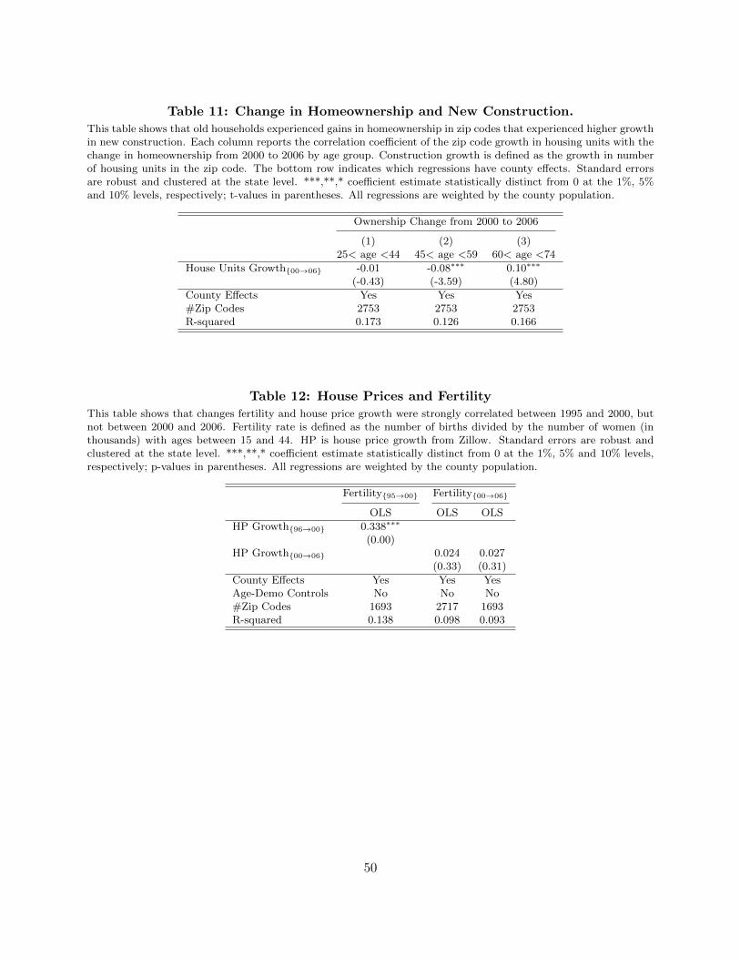
Table 11: Change in Homeownership and New Construction.

This table shows that old households experienced gains in homeownership in zip codes that experienced higher growthin new construction. Each column reports the correlation coefficient of the zip code growth in housing units with thechange in homeownership from 2000 to 2006 by age group. Construction growth is defined as the growth in numberof housing units in the zip code. The bottom row indicates which regressions have county effects. Standard errorsare robust and clustered at the state level. ***,**,* coefficient estimate statistically distinct from 0 at the 1%, 5%and 10% levels, respectively; t-values in parentheses. All regressions are weighted by the county population.

Ownership Change from 2000 to 2006

(1) (2) (3)25< age <44 45< age <59 60< age <74

House Units Growth{00→06} -0.01 -0.08∗∗∗ 0.10∗∗∗

(-0.43) (-3.59) (4.80)

County Effects Yes Yes Yes#Zip Codes 2753 2753 2753R-squared 0.173 0.126 0.166

Table 12: House Prices and Fertility

This table shows that changes fertility and house price growth were strongly correlated between 1995 and 2000, butnot between 2000 and 2006. Fertility rate is defined as the number of births divided by the number of women (inthousands) with ages between 15 and 44. HP is house price growth from Zillow. Standard errors are robust andclustered at the state level. ***,**,* coefficient estimate statistically distinct from 0 at the 1%, 5% and 10% levels,respectively; p-values in parentheses. All regressions are weighted by the county population.

Fertility{95→00} Fertility{00→06}

OLS OLS OLS

HP Growth{96→00} 0.338∗∗∗

(0.00)HP Growth{00→06} 0.024 0.027

(0.33) (0.31)

County Effects Yes Yes YesAge-Demo Controls No No No#Zip Codes 1693 2717 1693R-squared 0.138 0.098 0.093

50