moral hazard in credit markets: the incentive e⁄ect of ... · moral hazard in credit markets: the...

Moral Hazard in Credit Markets:

The Incentive Effect of Collateral

Marta Serra-Garcia∗

Tilburg University

October 25, 2010

JOB MARKET PAPER

Abstract

This paper examines the effect of collateral on moral hazard and credit volume. Astandard theoretical argument for the use of collateral is its power in reducing problemsof moral hazard. However, collateral may also be used as a screening device and existingempirical studies have not been able to isolate the incentive effect of collateral. Thispaper uses experimental tools to identify the effect. The results show that, contrary tothe theoretical predictions, collateral only decreases moral hazard when interest ratesare low. If interest rates are high, an increase in collateral does not decrease moralhazard significantly. The results suggest that borrowers’aversion to losses together withhigh interest rates offset the incentive effect of collateral. Furthermore, it is shown thatcollateral increases credit supply. But, if interest rates are high, increases in collateral alsolead to a decrease in credit demand. These findings suggest that the effects of collateraldepend on the interest rate charged and that these may be weaker than expected wheninterest rates are high.

Keywords: Collateral, Moral Hazard, Credit Access and Credit Markets.

JEL-Classification: C92, D23, G21, O16.

∗Author’s e-mail: [email protected] would like to thank Thorsten Beck, Martin Brown, Miguel Carvalho, Eric van Damme, Hans Degryse,

Peter Hoffmann, Wieland Mueller, Steven Ongena, Jan Potters, Abraham Ravid and Nathanael Vellekoopfor helpful comments and suggestions, and the audiences at the GSS seminar and Economics Workshopin Tilburg University, Brown Bag seminar at DICE (Duesseldorf University) and the doctoral tutorial ofthe 2010 EFA Meeting, at Goethe University Frankfurt.

1 Introduction

This paper provides the first systematic and direct evidence on the effect of collateral

on moral hazard and credit volume. Collateral is widely used in practice for financial

contracting. More than 80% of loans issued in the U.S (Berger et al, 2010) and more

than 75% of loans issued in over 100 countries, mainly developing economies (Chavis et

al, 2010), are collateralized. This widespread use of collateral has spurred a large, mainly

theoretical literature which aims at understanding loan collateralization.

A main theoretical motivation for the use of collateral is that it reduces moral hazard.

Models of lending under moral hazard predict that pledging collateral induces borrowers

to increase effort. Fear to lose the pledged asset increases the incentives to take costly

actions that increase the likelihood of repayment (e.g. Innes, 1990, Boot et al, 1991,

Besley and Ghatak, 2009a). Since collateral increases effort and thus profits from lending,

it may be a key determinant of a borrower’s access to credit.

Despite the important role of collateral in reducing problems of moral hazard, the

empirical evidence available is scarce. A problem faced by field data is that collateral may

also be used as a screening device. Investment projects of borrowers vary in quality, which

is often unknown to lenders. Since the quality of projects and actions of borrowers are

unobservable, the effect of collateral on moral hazard cannot be easily isolated. Recent

studies have used variations in the information on the quality of the loan at the moment

of extending a loan to identify the role of private information (Berger et al, 2010, Berger

et al, forthcoming). However, the effect of collateral on moral hazard, for a given project

quality, remains unknown.

Empirical evidence on the effect of collateral on credit access is also scarce and unex-

pectedly weak. Recent studies examine exogenous changes to property titles to evaluate

the impact of a title, which makes an asset pledgeable as collateral, on credit access.

Galiani and Schargrodsky (2010) do not find any increase in credit access after titles

have been extended in their Argentinian sample, while Field and Torero (2006) find that

credit access increases for public sector banks, but not for private sector banks in Peru.

It is unclear why credit access does not always increase. It may be that other enforce-

ment problems remain and that lenders fear not being able to seize assets upon default.

But it may also be that interest rates are too high. Surveys conducted by the World

Bank, described below, show that in many developing economies high interest rates are

the main reason for firms’lack of credit demand. Since interest rates are an important

determinant of credit demand, they may affect credit volume and interact with the effect

of collateral.

This study contributes to the existing literature by answering three questions using

experimental tools: does collateral decrease problems of moral hazard? Does collateral

2

affect credit supply, demand and ultimately credit volume? Do these effects depend on

an important loan characteristic, the interest rate?

The standard model of lending under moral hazard is simplified and implemented

experimentally. Each lender is matched with a borrower and decides whether or not he

offers a loan. If he offers a loan, he can request collateral. If the borrower accepts the

loan offer, she decides on her effort. Effort refers to all costly actions that increase the

probability of project success. It is not contractible and not observable to the lender

and thus the source of moral hazard. In line with the theoretical models cited above,

strategic default, an additional source of moral hazard, and other enforcement problems

are ruled out by design.

To identify the effect of collateral, the level of collateral is varied across treatments.

Two levels of collateral are considered: collateral that covers fifty percent of the loan

amount and collateral that fully covers the loan amount. Fully secured loans are very

common in loan contracts. The fifty percent case allows us to examine the effect of a

collateral increase towards a fully secured loan. At each level of collateral, the interest

rate is varied: a low and a high interest rate are considered. These values correspond to

the ex-ante optimal interest rates for the lender at each level of collateral. Varying the

level of collateral and the interest rate separately allows the identification of the effect

of each variable separately, while they are often observed jointly in the field. Further, a

benchmark treatment is added, in which borrowers do not have any collateral, to examine

the effect of collateral availability.

An increase in collateral is expected to increase the effort provided by borrowers. Since

collateral increases by the same amount at low and high interest rates, the same increase

in effort is expected. An increase in collateral is also expected to increase credit supply. In

particular, lenders are expected to supply credit when collateral can be pledged. However,

the effect of collateral on credit demand is ambiguous. If borrowers are risk neutral, they

are expected to always demand credit. However, if borrowers are risk averse, an increase

in collateral when interest rates are high may lead to a decrease in credit demand.

The first and most important experimental result is that the effect of collateral on

effort depends on the interest rate. At low interest rates, an increase in collateral increases

effort significantly. At high interest rates, it does not. Unexpectedly, the incentive effects

of collateral are weak when interest rates are high.

To further investigate this result, an additional treatment is added to the design.

The weak effect of collateral may be driven by borrowers’aversion to losses or by fairness

concerns. When collateral is large, a failure to repay the loan implies that the borrower

loses the asset pledged as collateral and faces the effort costs for the effort provided.

If interest rates are high, loss averse borrowers may not increase effort with collateral

3

increases since their profits in case of repayment are small. Alternatively, borrowers may

consider the loan offer unfair. A loan gives a large profit to the lender, while leaving the

borrower with little profit. By providing a low effort, borrowers decrease the lender’s

payoff advantage.

In the additional treatment, a tax on the lender’s profits is introduced to decrease

fairness considerations. The results reveal that the borrower’s effort remains low. This

suggests that borrowers’loss aversion together with high interest rates offsets the incen-

tive effect of collateral.

The second main finding is that credit supply increases with collateral. But, increases

in collateral lead to a decrease in credit demand, if interest rates are high. This decrease

in demand is related to borrowers’risk aversion, as hypothesized. Borrowers who are risk

averse are less likely to demand credit, if the interest rate is high and collateral increases.

These findings have two main implications. First, the incentive effect of collateral is

likely to be weak when interest rates are high. Borrowers’ concerns about losses may

imply that collateral does not lead to a substantial decrease in moral hazard in some

environments. Second, the effect of collateral on credit volume is also likely to be weak

in credit markets where interest rates are high. Although institutions are reformed to

improve property rights or to increase the use of collateral, if interest rates are high,

borrowers may be unwilling to demand credit.

The rest of the paper is organized as follows. In the next section, a brief overview

of the related literature and survey evidence is given. Then, the experimental design

is described. In Section 4, the experimental results are presented. Section 5 presents

additional results, which complement those of Section 4, and and Section 6 concludes.

2 Related literature and survey evidence

Why collateral is used and its effect on loan performance has been widely studied theoret-

ically in the banking literature. Several studies focus on the ex-ante effect of collateral.

In the presence of asymmetric information about the borrower quality, collateral has

an ex-ante effect on the pool of borrowers (e.g. Stiglitz and Weiss, 1981, Bester, 1985

and 1987). Other studies focus on the ex-post effect of collateral. Collateral provides

incentives for borrowers to act as desired by lenders, providing a high effort, as pointed

out, among others, by Innes (1990), Aghion and Bolton (1997), Holmstrom and Tirole

(1997), Mookherjee and Ray (2002) and Besley and Ghatak (2009a). These effects may

vary when the lending relationship is repeated as reputation concerns serve as an in-

centive to provide effort (Boot and Thakor, 1994). In this paper the focus is on the

direct effect of collateral and thus no reputation concerns are considered. Additionally,

4

collateral may also affect behavior of borrowers after receiving a loan in environments

where strategic default is possible (e.g. Banerjee and Newman, 1993) and under costly

state verification (e.g. Townsend, 1979). Some studies allow for both roles of collateral,

ex-ante and ex-post (Chan and Thakor, 1987, Boot et al, 1991).

Guided by existing theories, several studies examine the determinants of collateral em-

pirically, with the objective of distinguishing between these theories (Berger and Udell,

1990; Jimenez et al, 2006; Berger et al, 2010, Berger et al, forthcoming).1 A problem

is that the ex-ante and ex-post effects are diffi cult to tear apart because the borrower’s

quality and actions are both unobserved to the lender. Since they both affect the proba-

bility of default, one cannot directly identify the effect of collateral on moral hazard for

two projects of the same quality. In this paper, I concentrate on the problem of moral

hazard and provide, to the best of my knowledge, the first direct evidence on the effect of

collateral on moral hazard. 2 The experimental tools used in this paper contribute to a

small but increasing number of papers which use experimental methodologies to increase

our understanding of the microeconomics of banking (e.g. Brown and Zehnder, 2007 and

2010, and Fehr and Zehnder, 2009).

The incentive effect of collateral implies that collateral may be key for credit access.

Credit access in turn has important consequences for growth and development (Levine,

2005). De Soto (2001)3 therefore argues that the right institutions, in particular, property

rights sytems should be in place. Property titles allow individuals to pledge collateral,

among others (Besley and Ghatak, 2009b), and thus should be easy to access. Besley

and Ghatak (2009a) have studied the implications of this argument theoretically, while

Galiani and Schargrodsky (2010) and Field and Torero (2006) use natural experiments

to test it. Earlier papers have surveyed titled and untitled farmers (Carter and Olinto,

2003 and Feder et al, 1988). This paper complements the existing papers providing

experimental evidence on the effect of collateral on credit access.

While credit access is often determined by credit supply, lender’s willingness to

lend, the demand side is important too. As pointed out by Brown et al (forthcom-

ing) in Eastern European countries many firms who need credit choose not to demand it.

Taking a broader sample, from the Enterprise Surveys conducated by the World Bank

(www.enterprisesurveys.org), a similar result is obtained. This survey, conducted in 96

1Other studies consider the more general link between institutions, finance and development, byexamining how differences in creditor rights across countries affect the use of collateral (Liberti andMian, 2009).

2The only closely related study is Andreoni (2005). He studies experimentally the effect of implement-ing a ’satisfaction guaranteed’policy, by which principals can recover their payment if the agent fails toperform as they wish. This differs from the setup here, in that borrowers provide effort, which determinesthe probability of project success. The lender can therefore only receive the requested collateral if theproject fails and receives the interest if the project succeeds.

3See Woodruff (2001) for a review of de Soto’s (2001) book The Mystery of Capital.

5

countries, mainly developing economies, contains data about firms’access to credit and

credit needs. Of over 42,000 firms surveyed from 2006 to 2010, 62.8% report the need

for credit, but only 35.7% actually demand it. The reason for not demanding credit

which is mentioned most frequently is that interest rates were not favorable. Also, firms

mention complex application procedures and high collateral requirements as reasons for

not demanding credit. Further, firms, which demanded credit in the past and obtained

it, report that in more than 74% of the cases loans or lines of credit were collateralized.

The most frequent percentage of collateral relative to the loan amount was 100%.

This paper contributes to the literature and survey evidence by providing a systematic

study of the impact of collateral on moral hazard and credit volume using experimental

evidence.

3 Experimental design

3.1 Contracting under moral hazard

The standard model of moral hazard, in which collateral can be requested (see Innes,

1990), describes the following situation: a lender has funds available to lend to a borrower,

who needs a loan for an investment project. The borrower has some capital, which cannot

be used directly for investment but can be pledged as collateral. If the borrower receives

a loan, she starts an investment project, which requires her effort. Effort, which is costly

for the borrower, refers to all actions by the borrower which make the investment project

more likely to succeed. It is neither contractible nor observable by the lender. Thus, a

problem of moral hazard arises. The lender wishes a high effort from the borrower, since

it increases the likelihood of success and in turn repayment of the loan. By requesting

collateral, the lender incentivizes the borrower to provide a high effort, as she loses her

property if the project fails.

The standard model of moral hazard is implemented experimentally using a lending

game. The parameter values used in the experiment are used to describe the game,

except for the variables which vary across treatments: collateral, C, and repayment, R.

The lender (player L) has an initial amount of funds, his endowment, of 150. The

borrower, indexed as B, has an initial endowment of 100. The borrower’s initial endow-

ment cannot be used for investment. However, a part of it may be pledged as collateral,

0 ≤ C ≤ 100. By varying C the impact of institutional changes, which increase the

amount of pledgeable collateral, can be studied. These institutional changes may be

changes in the property rights system, which extend property titles on the borrower’s

endowment, or could also be changes in regulation, which increase the type of assets that

are pledgeable. Throughout, the value of collateral, C, is assumed to be the same for the

6

borrower and the lender, and no transaction costs or loss in collateral value ensue from

default.

The borrower’s investment project requires a loan of 100. If the project is successful,

it yields a return of 300. If it fails, it yields a return of zero. The sequence of moves in

the game is as follows. The lender and borrower are matched exogenously for one period

only. First, the lender decides whether or not to offer a loan, { offer, no offer}. If he

chooses to offer and collateral is available, the lender can choose to request collateral

or no collateral. To simplify notation, if the lender chooses no collateral, C is set to

0. Instead, when collateral is chosen, C is equal to the amount of collateral available.

By design, the lender does not decide on repayment, which is varied exogenously across

treatments. This allows evaluating the impact of the decision to request collateral on

effort, while keeping repayment constant. Repayment is set at the level which maximizes

the lender’s profits, as detailed below.

If the lender offers a loan, the borrower decides whether to accept or reject it. If she

accepts, the borrower decides on effort, e = {1, 2, 3, 4, 5}. Effort is costly, in monetaryterms, to the borrower: 4e2. The cost of effort is paid from a surplus of 100 that the

borrower receives when accepting a loan.4 Thus, the borrower’s net surplus from effort

is: S(e) = 100− 4e2. At the same time, effort increases the probability of success of theproject, by a factor of 16 , as shown in Table 1. None of the effort choices leads to a certain

project outcome.

Table 1: Effort, probability of success and surplus

Effort (e) 1 2 3 4 5

Probability of success 1/6 2/6 3/6 4/6 5/6

Surplus S(e) 96 84 64 36 0

If the lender decides not to offer a loan or the borrower rejects an offer, no loan

is extended. Then, the lender and borrower keep their initial endowments. If a loan

is offered and accepted, two outcomes are possible. First, if the project succeeds, the

lender is paid back repayment R, which includes the loan principal of 100 and an interest

payment. Thus, no strategic default is allowed. Second, the project may fail, in which

case the lender receives no repayment, but the requested collateral, C. This leads to the

following payoffs for the lender:

4Note that this surplus does not affect the borrower’s incentives, but only avoids net losses at the endof the game.

7

πL =

150 if no loan

50 +R if project succeeds

50 + C if project fails

The payoffs of the borrower are:

πB =

100 if no loan

100 + 300−R+ S(e) if project succeeds

100− C + S(e) if project fails

The expected payoff of a borrower who accepts a loan offer is

E(πB) = 100 +e

6(300−R)− (1− e

6)C + 100− 4e2

If the borrower is risk neutral, self-interested and rational, her optimal effort and

incentive compatibility constraint (ICC) is

e∗ =1

48(300−R+ C) (ICC)

The ICC reveals two comparative statics regarding the borrower’s effort. First, an

increase in collateral increases effort, ∂e∂C > 0, and this increase is independent of the

repayment, ∂2e∂C∂R = 0. Second, an increase in repayment decreases effort, ∂e

∂R < 0. Fur-

thermore, the borrower is willing to accept a loan offer, as long as

e

6(300−R)− (1− e

6)C + 100− 4e2 ≥ 0 (PC)

For a risk neutral, self-interested and rational lender, the maximization problem is

maxcollateral ,R

e

6R+ (1− e

6)C − 100

subject to the borrower’s incentive compatibility constraint (ICC), the borrower’s par-

ticipation constraint (PC) and his own participation constraint. Requesting collateral is

always optimal for the lender as the first derivative with respect to C is always positive.

The optimal interest rate is R = 150 + C. This interior solution is optimal for values of

collateral between 0 and 100. The intuition behind it is as follows. When the amount

of collateral is low, the incentive effect of collateral is also low. The borrower must pay

a low interest to have an incentive to provide a high effort. As the amount of collateral

comes closer to 100, a low interest becomes unnecessary. The larger amount of collateral

8

already provides the borrower with an incentive to exert effort. Thus, the lender can

charge a higher interest rate and still elicit a high effort.5

Given R∗ = 150+C, the lender’s participation constraint is satisfied if C ≥ 100−25 ·258 = 21

78 . Thus, for any C ≥ 21

78 , it is optimal for the lender to offer. For the borrower,

it is optimal to accept in all cases, as her PC has been taken into account. These results

yield Proposition 1. The proof is presented in Appendix A.

Proposition 1 If the lender and the borrower are risk neutral, an increase in collateralfrom 0 to 100% of the loan amount, has two main effects: (1) it reduces the problem

of moral hazard: effort supply increases; (2) it increases credit supply, while it does not

affect credit demand, and therefore it increases credit volume. Both effects do not vary

across different interest rate levels.

Proposition 1 highlights two main effects of collateral. First, pledging more collateral

reduces the problem of moral hazard. Second, pledging more collateral makes lending

profitable. This increases credit supply and since credit demand remains profitable,

it leads to an increase in credit volume. The second effect, however, hinges on the

assumption of risk neutral borrowers. Borrower risk aversion can lead to decreases in

credit demand as collateral increases. In particular, borrowers, who may lose their initial

endowment if the project fails, may be unwilling to take up a loan with a high interest and

high collateral. In contrast, for lenders, who have a larger endowment and always keep

part of it when lending, risk aversion is likely to play a minor role. Thus, the following

subsection examines the effect of borrower risk aversion.

3.2 The role of risk aversion

For a risk averse borrower, the expected utility from accepting a loan may be formulated

as follows E(uB) = e6 · u(100 + 300 − R) + (1 −

e6) · u(100 − C) + u(S(e)), where u(·)

is increasing, continuous and concave, and the surplus from effort is assumed to be

separable.

Risk aversion may decrease the borrower’s optimal effort. However, it is important

to note that, even if the borrower is risk averse, the effect of collateral on effort is still

independent of repayment. Collateral affects the borrower’s utility in the case of project

failure, while repayment affects utility in the case of project success. Thus, the effect of

collateral remains independent of the interest rate.

5This result, that the interest rate may increase with the amount of collateral pledged, is the same asin Besley and Ghatak (2009a), for the case of credit markets with monopolistic lenders.

9

In contrast, risk aversion leads to an interaction between the effect of collateral on

credit demand and repayment. If the interest rate on a loan is high and a large amount

of collateral must be pledged, a risk averse borrower may prefer to reject a loan offer and

have the certainty that she will keep her endowment of 100.

The effects of risk aversion are summarized in Proposition 2. The proof is presented

in Appendix A.

Proposition 2 If the borrower is risk averse, the effect of collateral on moral hazard re-mains independent of the interest rate. However, the effect of collateral on credit demand

may interact with the interest rate: credit demand is more likely to fall with collateral

increases at high interest rates.

Having clarified the role of risk aversion, we now turn to the specific treatments of

the experiment and derive hypotheses to be tested.

3.3 Treatments and Hypotheses

The experiment consists of four main treatments and one benchmark treatment. The

four main treatments allow for a 2x2 design, where the amount of collateral and the level

of interest are varied separately. Two levels of collateral are considered, 50% and 100%

of the loan amount. Also, two levels of interest payment are considered, low and high.

A low interest corresponds to the case where repayment is 200, while a high interest

corresponds to a repayment of 250. These are the optimal repayments for the lender

when collateral is 50 and 100, respectively.6

Table 2 displays the four treatments and the predicted effort level for risk neutral

borrowers. Risk aversion may change the exact effort predicted. However, the increase

in effort with an increase in collateral is still expected to be the same in Low and High

interest treatments. Since collateral is at least 50, offering and accepting a loan is optimal

in all treatments. Thus, all treatments are expected to feature a large credit volume.

Table 2: Experimental Treatments and Predictions

Interest

Low (R=200) High (R=250)

Collateral C=50 e∗ = 3 e∗ = 2

C=100 e∗ = 4 e∗ = 3

6Since repayment is the sum of loan principal and interest payment and the loan principal does notvary across treatments, an increase in repayment is equivalent to an increase in the interest. Therefore,these treatments are labelled as high interest and low interest.

10

A benchmark treatment is added to evaluate the impact of collateral availability. In

this treatment, labelled No Collateral, the amount of collateral is 0. Offering a loan is

not profitable and thus credit supply is expected to be zero. The repayment level is set

to R=200. The exact level of repayment does not affect predictions, as it is not profitable

to offer loans.

Two main hypotheses are tested. First, the effect of collateral on moral hazard is

expected to be as follows:

Hypothesis 1: If collateral increases, effort increases. The same increase is observedin Low and High Interest treatments.

Note that also if borrowers are risk averse such hypothesis is expected to hold.

The second hypothesis concerns credit volume. When collateral becomes available,

credit supply is expected to increase, since offering credit and requesting collateral is

optimal at collateral levels of 50 and 100, for both high and low interest. At the same

time, credit demand, which is always positive, does not vary.

Hypothesis 2: When collateral increases from C=0 to C=50 and C=100, credit volume

increases. Credit supply increases, while credit demand does not vary, both in Low and

High Interest treatments.

However, as we have seen, Hypothesis 2 may not be satisfied if borrowers are risk

averse. In that case, the effect of collateral availability on credit volume is expected to

depend on the interest rate. At high interest rates, an increase in collateral may decrease

credit demand. Thus, credit volume may fall with increases in collateral.

3.4 Procedures

The experiment was conducted in CentERlab at Tilburg University. In total 156 students

participated in the experiment. 28 in the treatment with C=100 and high interest, and 32

in all other treatments. Subjects only participated in one treatment. They were invited

via e-mail to participate in the experiment. The experiment was conducted using z-Tree

(Fischbacher, 2007).

Subjects started the lending game by reading a printed copy of the instructions (to

be found in Appendix B). After all subjects had read the instructions, they were asked

to fill in a quiz that was then checked by the experimenter. The labeling of the game was

neutral. Each subject was assigned the role of player 1 or player 2, lender or borrower

respectively, from the start. Player 1 could offer 100 points to player 2 and, in the

treatments with available collateral, player 1 could request collateral. To simplify the

11

borrower’s task in the experiment and make sure the effect of effort on the probability of

success was clear, the borrower’s task in the investment project consisted in buying red

balls. At the start, there were 6 black balls in the project. Player 2 could choose how

many red balls to buy (1, 2, 3, 4 or 5) and each red ball substituted a black ball. Black

and red balls represented project failure and success, respectively. Therefore, subjects

could easily understand that by buying more balls, they were increasing the chances of

project success. Buying red balls was costly for the borrower. The borrower was clearly

informed about these costs (in the instructions and computer screens).

The game was played once. This prevented wealth effects, which may influence bor-

rowers’perception of collateral pledging over time and thus incentives. It also prevented

group reputation effects from influencing lenders’and borrowers’decisions. To elicit bor-

rowers’decisions the strategy method was used. That is, each borrower decided to accept

or reject a loan offer and her effort, before knowing the lender’s offer. This method pro-

vides a within-subject measure of the effect of collateral requests, i.e. borrower decisions

are observed for both the case that the lender requests collateral and the case that he

does not. After the effort decision, the decisions of the lender and borrower were com-

bined (within each pair) and the computer made a random draw from the distribution,

determined by the effort choice of the borrower.

Each session started with three pre-experimental games: a risk preference elicitation

task (which is a variation of Holt and Laury, 2002), a p-beauty contest game with p=23

(Nagel, 1995) and a trust game (Berg et al, 1995). These games, which were played

without any feedback, yield measures related to risk preferences, rationality and social

concerns. These can then be used as controls on behavior in the lending game.7 After

the lending game, subjects’beliefs about others’behavior were elicited. Subjects were

rewarded monetarily, depending on the distance between their belief and the actual

average behavior of others.

At the end of the experiment, they were informed about the outcome of each pre-

experimental game, the lending game and the accuracy of their beliefs.8 Subjects were

then paid their earnings in private and in cash. Average total earnings were 10.5 EUR.

Of these, the largest portion was earned in the lending game, 6.6 EUR. The experiment

lasted 45 to 60 minutes.7Appendix C.1 presents a detailed description of these games and summary statistics.8Beliefs were close to actual behavior of other players. A detailed summary of beliefs compared to

actual behavior is provided in Appendix C.2.

12

4 Results

In this section, the effect of collateral on effort is analyzed first. Then, the results on

credit supply, demand and volume are presented. The profits obtained across treatments

are reported thereafter.

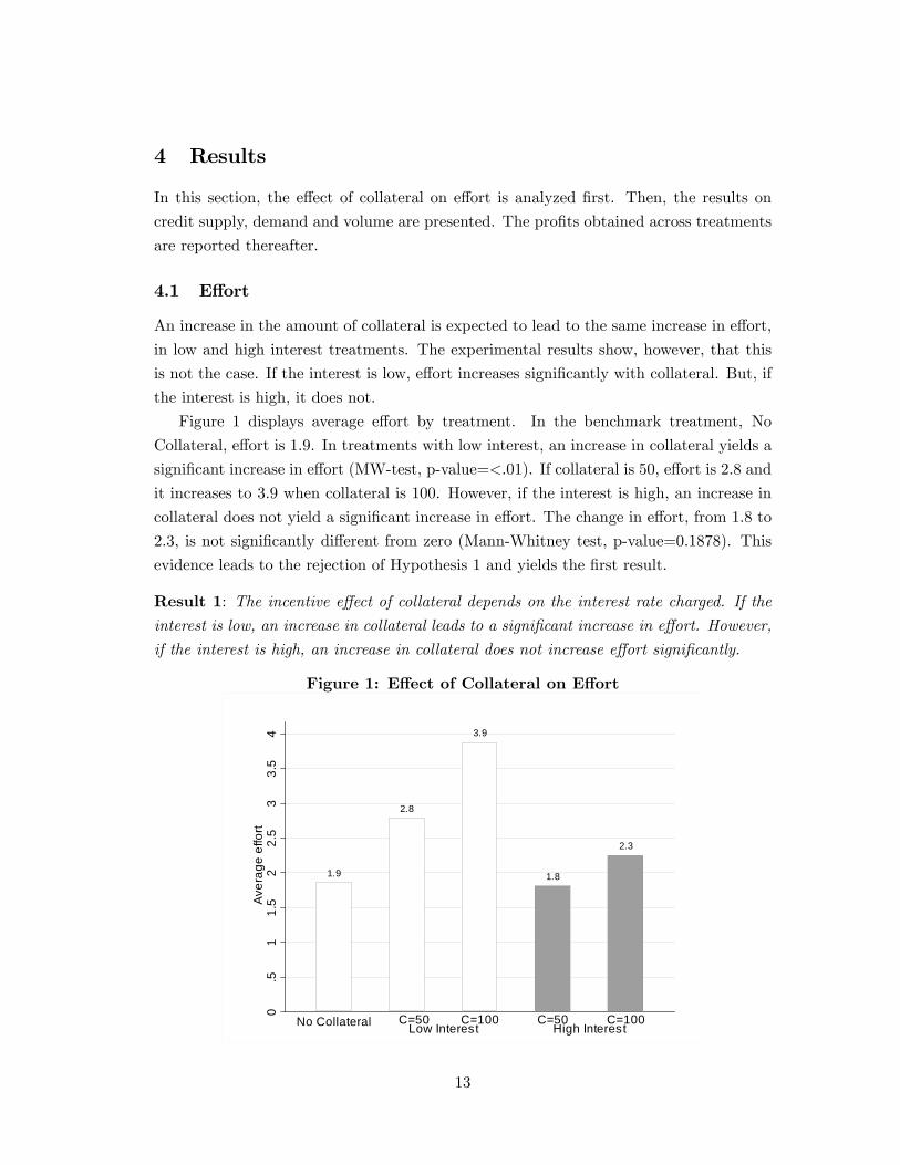
4.1 Effort

An increase in the amount of collateral is expected to lead to the same increase in effort,

in low and high interest treatments. The experimental results show, however, that this

is not the case. If the interest is low, effort increases significantly with collateral. But, if

the interest is high, it does not.

Figure 1 displays average effort by treatment. In the benchmark treatment, No

Collateral, effort is 1.9. In treatments with low interest, an increase in collateral yields a

significant increase in effort (MW-test, p-value=<.01). If collateral is 50, effort is 2.8 and

it increases to 3.9 when collateral is 100. However, if the interest is high, an increase in

collateral does not yield a significant increase in effort. The change in effort, from 1.8 to

2.3, is not significantly different from zero (Mann-Whitney test, p-value=0.1878). This

evidence leads to the rejection of Hypothesis 1 and yields the first result.

Result 1: The incentive effect of collateral depends on the interest rate charged. If theinterest is low, an increase in collateral leads to a significant increase in effort. However,

if the interest is high, an increase in collateral does not increase effort significantly.

Figure 1: Effect of Collateral on Effort

1.9

2.8

3.9

1.8

2.3

No Collateral C=50 C=100 C=50 C=100Low Interest High Interest

0.5

11.

52

2.5

33.

54

Ave

rage

effo

rt

13

When the interest is high and C=100, effort is unexpectedly low. The average effort

is 2.3, while we would expect it to be 3. As will be shown below, in this treatment lenders

always request collateral. Thus, the low effort cannot stem from the lack of collateral

requests. It is rather borrowers who are not strongly responding to the incentives of

collateral. Comparing effort for the case that the lender requests collateral and the case

that he does not, confirms the weak response to incentives. Table 3 presents average

effort in each case, for all treatments in which collateral is available.

Table 3: Effort response to a request to pledge collateral

Collateral Low Interest High Interest

C=50 Effort if no collateral requested 2.2 1.2

Effort if collateral requested 2.9 1.8

WSR-test (p-value) <.01 <.01

C=100 Effort if no collateral requested 2.6 1.3


WSR-test (p-value) 0.01 0.07

Note: WSR-test is the non-parametric Wilcoxon signed ranks test.

If C=50, effort when collateral is requested is significantly higher than when it is

not, both with low and high interest. This is revealed by the p-value of the WSR-test,

which is lower than .01 in both cases. The same result is obtained when C=100 and the

interest is low. In contrast, the effect of a collateral request is weaker when the interest

and collateral are high. In that case, effort displays a small increase, from 1.29 to 2.25,

which is marginally significant, p=0.07.

A regression analysis of effort decisions is shown in Table 4, which reports OLS

estimation results for the determinants of effort. These results are presented for the case

that the interest is low (columns 1 and 2), if it is high (columns 3 and 4) and pooling both

cases (columns 5 and 6). Treatment dummies and a dummy for the case the collateral

is requested are considered first. Individual characteristics are added subsequently. Also

the interaction term between high interest and risk aversion is included. This term allows

us to examine whether the effect of risk aversion is independent of the interest rate.

When the interest payment is low, requesting a larger amount of collateral, 100 com-

pared to 50, increases the effort level significantly. This can be seen from the positive and

significant coeffi cient of the variable Collateral=100 in columns 1 and 2. However, if the

interest payment is high, this effect is no longer observed (columns 3 and 4). Increasing

the amount of collateral does not increase effort as already revealed by Figure 2.

14

Table 4: Determinants of effort

(1) (2) (3) (4) (5) (6)

Low Interest High Interest All

Collateral=100 0.688** 0.511* 0.240 0.282 0.688** 0.582**

[0.262] [0.277] [0.203] [0.194] [0.260] [0.265]

High Interest -1.063*** -1.088***

[0.235] [0.260]

C=100;High Interest -0.430 -0.215

[0.326] [0.325]

Collateral Requested 1.000*** 1.000*** 0.757*** 0.752*** 0.891*** 0.885***

[0.262] [0.271] [0.174] [0.172] [0.164] [0.167]

Risk aversion -0.333 -0.234 -0.288

[0.289] [0.172] [0.300]

Risk aversion*High Int. -0.013

[0.360]

Strategic Reasoning -0.004 0.007 0.005

[0.010] [0.005] [0.006]

Trust -0.049 0.005 -0.023

[0.040] [0.024] [0.025]

Trustworthiness 0.027 -0.006 0.010

[0.045] [0.027] [0.028]

Constant 2.063*** 2.623*** 1.122*** 0.674 2.117*** 1.918***

[0.249] [0.722] [0.140] [0.402] [0.223] [0.445]

Observations 64 64 54 54 118 118

Number of subjects 32 32 30 30 62 62

R-squared 0.263 0.289 0.264 0.309 0.490 0.502

Note: this table reports OLS regression estimates for effort, the dependent variable. The

variable Collateral=100 is a dummy variables that takes value 1 if C=100; High Interest

takes value 1 if R=250; C=100;High Interest is the interaction term between C=100 and

High Interest. Collateral Requested takes value 1 if the lender choose to request collateral.

Risk aversion, Strategic Reasoning,Trust and Trustworthiness are measures from the

pre-experimental games. Risk aversion*High Int. is the interaction term between risk

aversion and High Interest.*** p<0.01, ** p<0.05, * p<0.1; Clustered standard errors at the

subject level in brackets.

When both levels of the interest payment are combined (columns 5 and 6), we observe

that the coeffi cient Collateral=100 is significantly positive, but the sum of this coeffi cient

and that of C=100*R=250 is not significantly different than 0 (F-test, p-value=0.1643).

15

This confirms that collateral increases lead to an increase in effort when the interest is

low, but not when it is high. Individual characteristics, including risk aversion and its

interaction with the interest level, do not affect effort decisions significantly.

These results confirm that the incentive effect of collateral depends on the interest

rate. Nevertheless, they do not clarify why this is the case. Two potential explanations

can be given. First, borrowers may not be willing to take up a loan when project failure

may leave them with a lower payoff than their initial endowment. If the project fails,

they not only lose their collateral but also face the effort cost. Borrowers who are averse

to this loss may choose a low effort to save on effort costs, when the interest is high. In

contrast, when the interest is low, payoffs from success compensate the loses in case of

project failure and incentivize borrowers to exert a high effort.

Second, borrowers may perceive a high payoff obtained by the lender as unfair. When

the interest is high, the lender’s payoff advantage is largest. Borrowers may decrease it

by decreasing their effort. These two explanations are detailed in the next section, which

presents results from an additional treatment aimed at distinguishing between them.

4.2 Credit volume

Figure 2 displays credit volume per treatment. In the absence of collateral, 44% of all

possible loans are offered and accepted. This volume of credit increases up to 100% when

collateral becomes available. However, the increase in credit volume is not independent of

the interest rate. When the interest rate is high, credit volume drops from 100% to 57%

when collateral increases from C=50 to C=100. Therefore, the flow of credit not only

depends on collateral availability, but is also sensitive to the particular loan conditions.

The differences in credit volume across treatments can be better understood by con-

sidering credit demand and supply separately. The increase in credit volume, when the

interest is low, is driven by credit supply. In contrast, the decrease, when interest is

high, is driven by credit demand. Table 5 displays credit demand and supply in each

treatments.

16

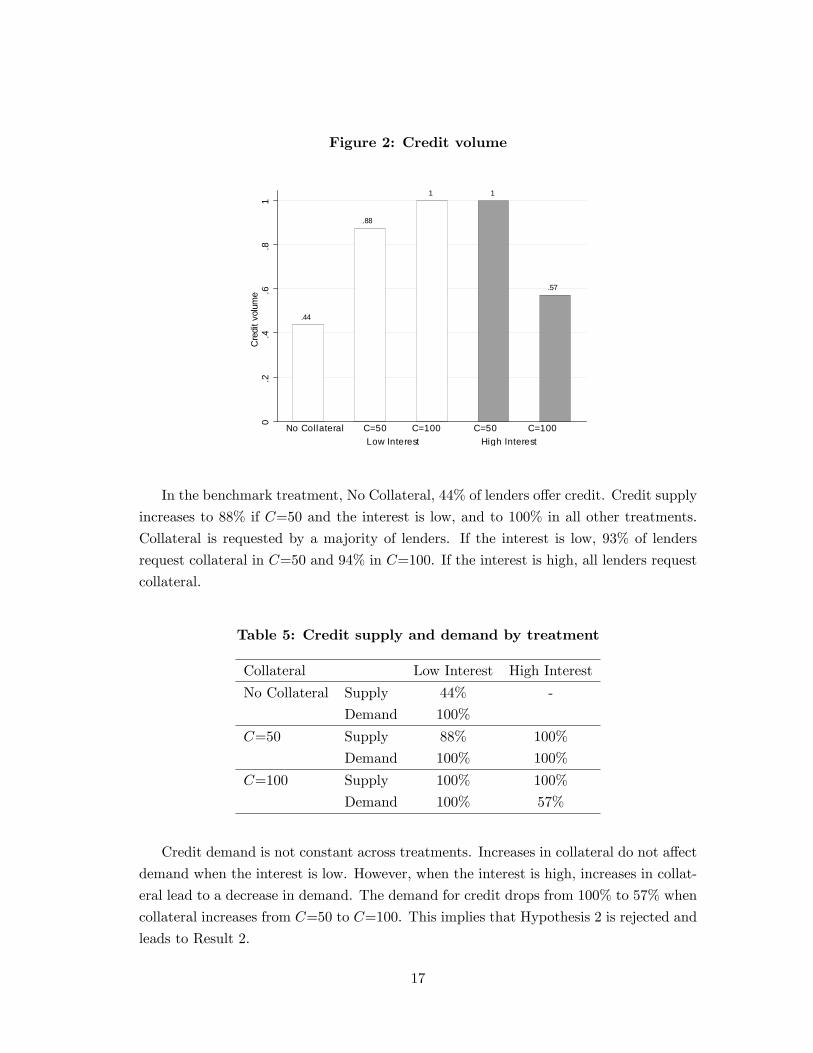
Figure 2: Credit volume

.44

.88

1 1

.57

No Collateral C=50 C=100 C=50 C=100Low Interest High Interest

0.2

.4.6

.81

Cre

dit v

olum

e

In the benchmark treatment, No Collateral, 44% of lenders offer credit. Credit supply

increases to 88% if C=50 and the interest is low, and to 100% in all other treatments.

Collateral is requested by a majority of lenders. If the interest is low, 93% of lenders

request collateral in C=50 and 94% in C=100. If the interest is high, all lenders request

collateral.

Table 5: Credit supply and demand by treatment

Collateral Low Interest High Interest

No Collateral Supply 44% -

Demand 100%

C=50 Supply 88% 100%

Demand 100% 100%

C=100 Supply 100% 100%

Demand 100% 57%

Credit demand is not constant across treatments. Increases in collateral do not affect

demand when the interest is low. However, when the interest is high, increases in collat-

eral lead to a decrease in demand. The demand for credit drops from 100% to 57% when

collateral increases from C=50 to C=100. This implies that Hypothesis 2 is rejected and

leads to Result 2.

17

Result 2: If collateral increases, credit supply increases both with high and low in-terest rates. However, at high interest rates, an increase in collateral decreases credit

demand.

Therefore, we observed the predicted increase in credit supply with increases in col-

lateral. However, there is one surprising result. In the treatment without collateral,

offering a loan is not profitable. Nevertheless, a substantial portion of lenders offer loans.

This may be driven by lender’s trust towards borrowers. Trusting borrowers would be

consistent with the presence of trust in many investment environments, in particular

in microfinance and venture capital markets (Bottazzi et al, 2010). Such relationship

between trust and offers in the absence of collateral is also found among the experimen-

tal subjects. The Spearman rank correlation coeffi cient between trust and offers in No

Collateral is positive and significant, 0.4789 (p-value=0.0605). Also, trust is the only

individual characteristic which is signficantly correlated to credit offers.

Further, we observe that at high interest rates demand decreases with collateral. As

studied above, this may be caused by risk aversion. The data reveal that risk averse

borrowers are slightly more likely to reject credit offers, though the relationship is not

significant (Fisher’s exact test, p-value=0.238). A caveat is that in this treatment the

share of risk averse borrowers is higher than in others. 57% of the borrowers are risk

averse while in other treatments the share of risk averse borrowers is at most 31%.

Due to the limited variation of credit demand in other treatments, it is not possible to

directly address this difference in the rate of risk averse borrowers with the existing data

and conduct an econometric analysis of demand. However, results from an additional

treatment, presented in the next section, will provide the additional data to perform this

analysis.

4.3 Payoffs

The incentive effects of collateral have consequences on lender, borrower and total pay-

offs. More collateral increases the lender’s payoff, though it does not always increase

the borrower’s payoff. Table 6 below displays expected payoffs, using the decisions of

players and calculating the expected payoff based on the probability of success. Realized

payoffs are basically the same for most of the treatments, where the average of all draws

corresponds to the expectation, except for the treatment with low interest and C=50,

where draws were unexpectedly lucky.

Starting with the lender, his payoff is lowest when no collateral is available. In this

treatment 44% of lenders offer a loan. Doing so is unprofitable, since borrowers exert

a low effort. The lender’s payoff increases with collateral, both in treatments with high

18

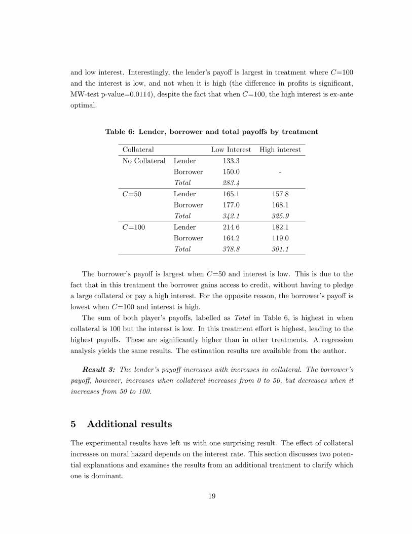
and low interest. Interestingly, the lender’s payoff is largest in treatment where C=100

and the interest is low, and not when it is high (the difference in profits is significant,

MW-test p-value=0.0114), despite the fact that when C=100, the high interest is ex-ante

optimal.

Table 6: Lender, borrower and total payoffs by treatment

Collateral Low Interest High interest

No Collateral Lender 133.3

Borrower 150.0 -

Total 283.4

C=50 Lender 165.1 157.8

Borrower 177.0 168.1

Total 342.1 325.9

C=100 Lender 214.6 182.1

Borrower 164.2 119.0

Total 378.8 301.1

The borrower’s payoff is largest when C=50 and interest is low. This is due to the

fact that in this treatment the borrower gains access to credit, without having to pledge

a large collateral or pay a high interest. For the opposite reason, the borrower’s payoff is

lowest when C=100 and interest is high.

The sum of both player’s payoffs, labelled as Total in Table 6, is highest in when

collateral is 100 but the interest is low. In this treatment effort is highest, leading to the

highest payoffs. These are significantly higher than in other treatments. A regression

analysis yields the same results. The estimation results are available from the author.

Result 3: The lender’s payoff increases with increases in collateral. The borrower’spayoff, however, increases when collateral increases from 0 to 50, but decreases when it

increases from 50 to 100.

5 Additional results

The experimental results have left us with one surprising result. The effect of collateral

increases on moral hazard depends on the interest rate. This section discusses two poten-

tial explanations and examines the results from an additional treatment to clarify which

one is dominant.

19

As mentioned before, borrowers’ loss aversion or fairness concerns could affect the

impact of collateral on moral hazard. Suppose borrowers are loss averse. A simple

utility function that captures loss aversion is proposed by Kahneman and Tversky (1979).

Utility is experienced by borrowers in terms of changes with respect to a reference point

x. Thus, the borrower’s utility depends on the difference between her final payoff πB and

this reference point,

U(x) =

πB − x if πB − x ≥ 0

λ(πB − x) if πB − x < 0

where λ > 1. In the lending game a natural reference point is the borrower’s initial

endowment, 100 points. In treatment No Collateral and treatments with C=50, at most

50 points are pledged and effort supply is at most 3. Thus, the loss domain (where

uB − x < 0) is not entered. In contrast, in treatments where C=100, borrowers may

enter in the loss domain. If the project fails, borrowers transfer their complete initial

endowment of 100 points to the lender. Since they must provide effort of at least one,

effort costs are perceived as losses. Importantly, the effect of loss aversion differs across

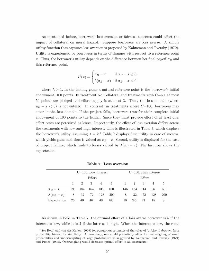
the treatments with low and high interest. This is illustrated in Table 7, which displays

the borrower’s utility, assuming λ = 2.9 Table 7 displays first utility in case of success,

which yields gains and thus is valued as πB − x. Second, utility is displayed for the caseof project failure, which leads to losses valued by λ(πB − x). The last row shows the

expectation.

Table 7: Loss aversion

C=100, Low interest C=100, High interest

Effort Effort

1 2 3 4 5 1 2 3 4 5

πB − x 196 184 164 136 100 146 134 114 86 50

λ(πB − x) -8 -32 -72 -128 -200 -8 -32 -72 -128 -200

Expectation 26 40 46 48 50 18 23 21 15 8

As shown in bold in Table 7, the optimal effort of a loss averse borrower is 5 if the

interest is low, while it is 2 if the interest is high. When the interest is low, the rents9See Booij and van der Kuilen (2009) for population estimates of the value of λ. Also, I abstract from

probability biases, for simplicity. Alternatively, one could potentially allow for overweighing of smallprobabilities and underweighting of large probabilities as suggested by Kahneman and Tversky (1979)and Prelec (1998). Overweighing would decrease optimal effort in all treatments.

20

from success are large, and therefore the borrower has an incentive to exert a high effort

to obtain those payoffs and avoid losing her capital. In contrast, with high interest, the

rents from success are small and the borrower is no longer as strongly motivated to make

the project succeed but to reduce the losses from failure. This diminishes effort supply

to 2.

Alternatively, suppose the borrower has fairness concerns. A simple way to model

these is using the inequity aversion model by Fehr and Schmidt (1999). In this model, the

utility of the borrower over each pair of final payoffs is U(πB, πL) = πB−αBmax{0, πL−πB} − βBmax{0, πB − πL}, where αB ≥ βB, and 0 ≤ βB < 1.10 It is easy to show that

lower levels of αB are needed for the borrower to be willing to lower her effort supply

when collateral is 100 and the interest is high, compared to when the interest is low.

Thus, fairness concerns could explain the low effort in under high interest and collateral.

A potential concern in comparing low and high interest rate treatments, when C=100,

is that acceptance varies across treatments, as fewer borrowers demand credit when

C=100 and the interest is high. This could lead to differences in the risk aversion of

borrowers who accept a loan. Nevertheless, selection works against lower effort. Suppose

risk averse borrowers reject offers when C=100 and the interest are high, while they

accept offers when C=100 but the interest low. Then the pool of borrowers who demand

credit is likely to be less risk averse when the interest rate is high. Thus, when C=100

and interest rates are high, we would not expect a lower effort .

A Tax treatment allows us to disentangle between loss aversion and fairness concerns.

This treatment is identical to that with C=100 and high interest, but for a tax on the

lender’s profits of 75 points if the project succeeds. This tax decreases the difference

between the lender and borrower’s payoffs and therefore strongly reduces the role of

fairness. In fact, it makes payoff differences very close to those in the treatment with

C=100 and low interest, where effort is very close to the prediction. Alternatively, one

could also consider a treatment which reduces loss concerns. But doing so is diffi cult.

For example, changing the borrower’s endowment not only changes the reference point

but also the borrower’s participation constraint.

Effort in the additional Tax treatment is presented in Table 8. Effort with and without

the tax is similar in both treatments. Importantly, when collateral is requested, effort is

10Note that inequity aversion is a model that generates spiteful behavior when a player is at a payoffdisadvantage. Such spiteful behavior may also be generated by different models, such as Levine (1998).In his model there are altruistic, selfish and spiteful types, which are unidentifiable ex-ante. A player’sutility depends on other’s types in the following way: Ui = ui +

ai+λaj1+λ

uj , where ui is the player’s ipayoff, -1 < ai ≤ 1 is the coeffi cient of altruism of player i and λ the weight player i assigns to player j’stype. Note that in our experiment most lenders offer loans and request collateral and thus their behavioris consistent with that of a pooling equilibrium (all types choosing the same action). As a consequence,the borrower’s perception of aj is most likely equal to the population average, a. Therefore, we are leftwith a parameter which is very similar to that of inequity aversion, and can be simplified to αi(ai, λ, a).

21

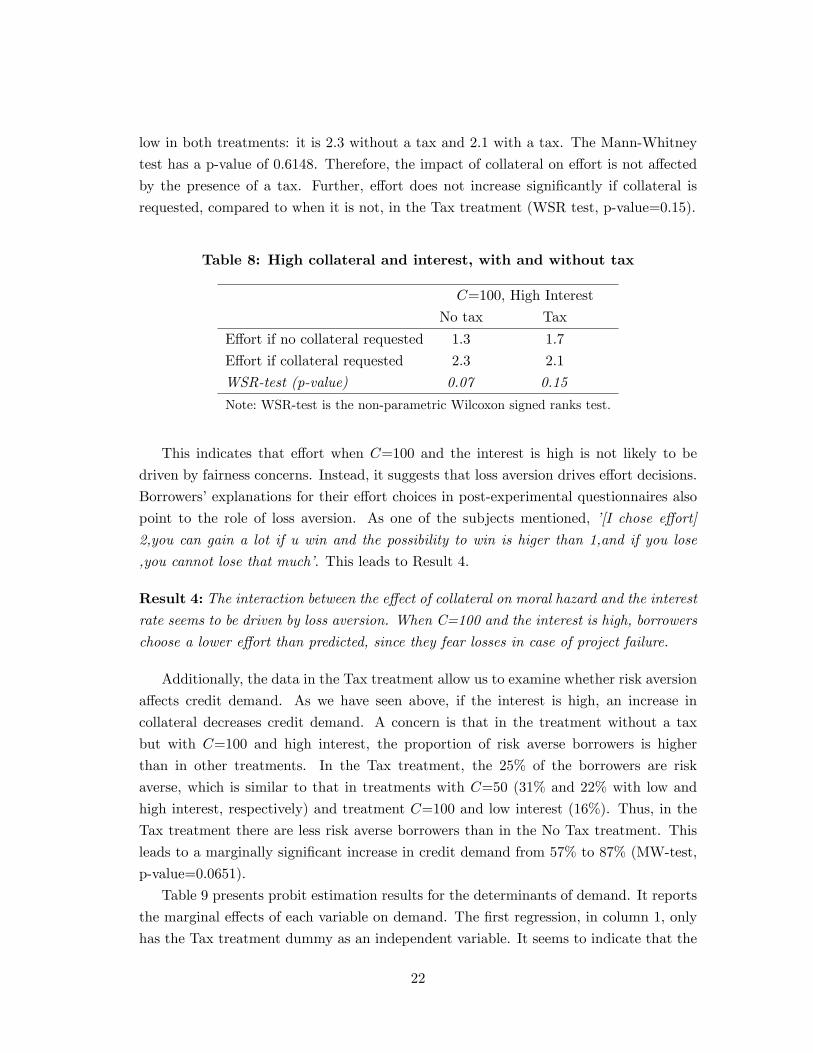
low in both treatments: it is 2.3 without a tax and 2.1 with a tax. The Mann-Whitney

test has a p-value of 0.6148. Therefore, the impact of collateral on effort is not affected

by the presence of a tax. Further, effort does not increase significantly if collateral is

requested, compared to when it is not, in the Tax treatment (WSR test, p-value=0.15).

Table 8: High collateral and interest, with and without tax

C=100, High Interest

No tax Tax

Effort if no collateral requested 1.3 1.7


WSR-test (p-value) 0.07 0.15

Note: WSR-test is the non-parametric Wilcoxon signed ranks test.

This indicates that effort when C=100 and the interest is high is not likely to be

driven by fairness concerns. Instead, it suggests that loss aversion drives effort decisions.

Borrowers’explanations for their effort choices in post-experimental questionnaires also

point to the role of loss aversion. As one of the subjects mentioned, ’[I chose effort]

2,you can gain a lot if u win and the possibility to win is higer than 1,and if you lose

,you cannot lose that much’. This leads to Result 4.

Result 4: The interaction between the effect of collateral on moral hazard and the interestrate seems to be driven by loss aversion. When C=100 and the interest is high, borrowers

choose a lower effort than predicted, since they fear losses in case of project failure.

Additionally, the data in the Tax treatment allow us to examine whether risk aversion

affects credit demand. As we have seen above, if the interest is high, an increase in

collateral decreases credit demand. A concern is that in the treatment without a tax

but with C=100 and high interest, the proportion of risk averse borrowers is higher

than in other treatments. In the Tax treatment, the 25% of the borrowers are risk

averse, which is similar to that in treatments with C=50 (31% and 22% with low and

high interest, respectively) and treatment C=100 and low interest (16%). Thus, in the

Tax treatment there are less risk averse borrowers than in the No Tax treatment. This

leads to a marginally significant increase in credit demand from 57% to 87% (MW-test,

p-value=0.0651).

Table 9 presents probit estimation results for the determinants of demand. It reports

the marginal effects of each variable on demand. The first regression, in column 1, only

has the Tax treatment dummy as an independent variable. It seems to indicate that the

22

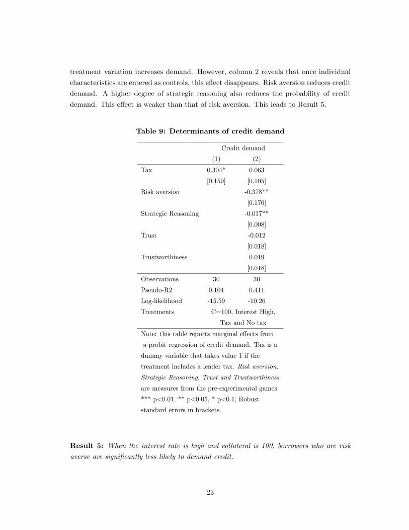
treatment variation increases demand. However, column 2 reveals that once individual

characteristics are entered as controls, this effect disappears. Risk aversion reduces credit

demand. A higher degree of strategic reasoning also reduces the probability of credit

demand. This effect is weaker than that of risk aversion. This leads to Result 5.

Table 9: Determinants of credit demand

Credit demand

(1) (2)

Tax 0.304* 0.063

[0.159] [0.105]

Risk aversion -0.378**

[0.170]

Strategic Reasoning -0.017**

[0.008]

Trust -0.012

[0.018]

Trustworthiness 0.019

[0.018]

Observations 30 30

Pseudo-R2 0.104 0.411

Log-likelihood -15.59 -10.26

Treatments C=100, Interest High,

Tax and No tax

Note: this table reports marginal effects from

a probit regression of credit demand. Tax is a

dummy variable that takes value 1 if the

treatment includes a lender tax. Risk aversion,

Strategic Reasoning, Trust and Trustworthiness

are measures from the pre-experimental games

*** p<0.01, ** p<0.05, * p<0.1; Robust

standard errors in brackets.

Result 5: When the interest rate is high and collateral is 100, borrowers who are riskaverse are significantly less likely to demand credit.

23

6 Conclusion

Understanding the role of collateral in credit markets is very relevant. Collateral is

widely used in financial contracting and can have important consequences for growth

and the persistence of income inequality. Several theoretical models have studied the

role of collateral. Many have pointed out the effect of collateral in reducing moral hazard

and the implications this has for credit supply. However, the empirical evidence of the

effect of collateral on moral hazard is scarce. This paper contributes to the literature

by providing the first experimental evidence regarding the effect of collateral on moral

hazard and credit volume.

A main contribution of the paper is to identify the direct effect of collateral on bor-

rower effort. The main finding is that, contrary to the theoretical predictions, the effect

of collateral on effort depends on the interest rate. In markets with low interest rates,

increases in collateral have a strong effect on effort. In contrast, in markets with high in-

terest rates, the effect of collateral increases is weak. When the amount of collateral and

the interest rate are high, borrowers provide an unexpectedly low effort. Results from

an additional treatment suggest that this effect is caused by borrowers’loss aversion. In

taking up a loan with high collateral, borrowers face the risk of losing their initial wealth

and paying effort costs as well. When the interest rate is high, loss averse borrowers

prefer providing a low effort to save on effort costs.

A second important contribution of the paper is to identify the effect of collateral

on credit supply and demand. As many theoretical studies have pointed out: increases

in collateral, make lending more profitable as they reduce the problem of moral hazard.

Thus, credit supply should increase with collateral availability. The experimental results

confirm such prediction. The results also point out that credit demand may depend on

collateral requirements. As pointed out theoretically in the paper, if borrowers are risk

averse, increases in collateral availability may decrease credit demand, especially if the

interest rate is high. The experimental results reveal that risk aversion has such effects

on credit demand.

The results indicate that the effects of collateral, on moral hazard and credit volume,

are likely to be strongest in markets with low interest rates. In these markets, the

incentive effect of collateral is likely to reduce loan defaults significantly. Additionally,

the availability of collateral is likely to increase credit volume strongly, as it increases

credit supply and does not decrease credit demand. Thus, institutional changes which

allow more assets to be pledged as collateral, such as reforms which make property

registration easier or directly extend property titling, are likely to be most effective in

markets where interest rates are low.

Finally, the results also indicate that borrower behavior may be driven by concerns

24

about risk and losses. Risk concerns decrease credit demand, especially when interest

rates are high. This provides an explanation for the low credit demand in developing

economies, despite the need of credit. Managers of small and medium enterprises, who

indicate that high interest rates are the main reason for their lack of demand, may be

averse to the risks of borrowing. Further, the experimental results reveal that borrower

behavior, after a loan has been extended, may also be affected by concerns about losses.

If loans feature high interest rates and are fully secured, borrowers may choose to save

on effort costs rather than provide a high effort. This may substantially weaken the

incentive effect of collateral on moral hazard.

25

Appendix A: Proofs

Proposition 1 If the lender and the borrower are risk neutral, an increase in collateralfrom 0 to 100% of the loan amount, has two main effects: (1) it reduces the problem

of moral hazard: effort supply increases; (2) it increases credit supply, while it does not

affect credit demand, and therefore it increases credit volume. Both effects do not vary

across different interest rate levels.

Proof. If the borrower is risk averse, increases in collateral decrease the problem of moralhazard, independently of the interest rate. However, at high interest rates, increases in

collateral may decrease credit demand.e∗ = 148(300 − R + C), ∂e

∂C > 0 and ∂2e∂C∂R = 0.

The second effect of collateral follows from the fact that, given R∗ = 150 + C, the

lender’s participation constraint is satisfied if C ≥ 2178 , and the borrower’s participationis satisfied for all 0≤ C ≤ 100.

Proposition 2 If the borrower is risk averse, the effect of collateral on moral hazard re-mains independent of the interest rate. However, the effect of collateral on credit demand

may interact with the interest rate: credit demand is more likely to fall with collateral

increases at high interest rates.

Proof. The partial derivative of utility with respect to effort is

∂U

∂e= g[u(100 + 300−R)− u(100− C)]− 8eu′(100− 4e2) (1)

We have that the optimal effort is determined by 8eu′(100− 4e2) = g[u(100+300−R)−u(100−C)]. It follows that an increase in collateral (C) increases the optimal effort level.Furthermore, this effect is independent of R. 11

Additionally, borrower’s participation constraint is

e

6· u(100 + 300−R) + (1− e

6) · u(100− C) + u(S(e)) ≥ u(100)

Suppose a risk neutral borrower’s participation is satisfied with equality for a given R

and C=100. Then, it follows that the participation constraint of a risk averse borrower,

for the same R and C is violated.11Note that, in general, risk aversion decreases the optimal effort provided by the borrower. This can

be seen from the fact that the right-hand side of 8eu′(100 − 4e2) = g[u(100 + 300 − R) − u(100 − C)]decreases due to risk aversion. Therefore, the left hand side must decrease as well. This is achieved onlyif effort decreases. We have that ∂

∂e8eu′(100 − 4e2) = 8[u′(100 − 4e2) − 8e2u′′(100 − 4e2)] > 0, since

u′′(100− 4e2) < 0 by concavity. Thus risk aversion decreases effort.

26

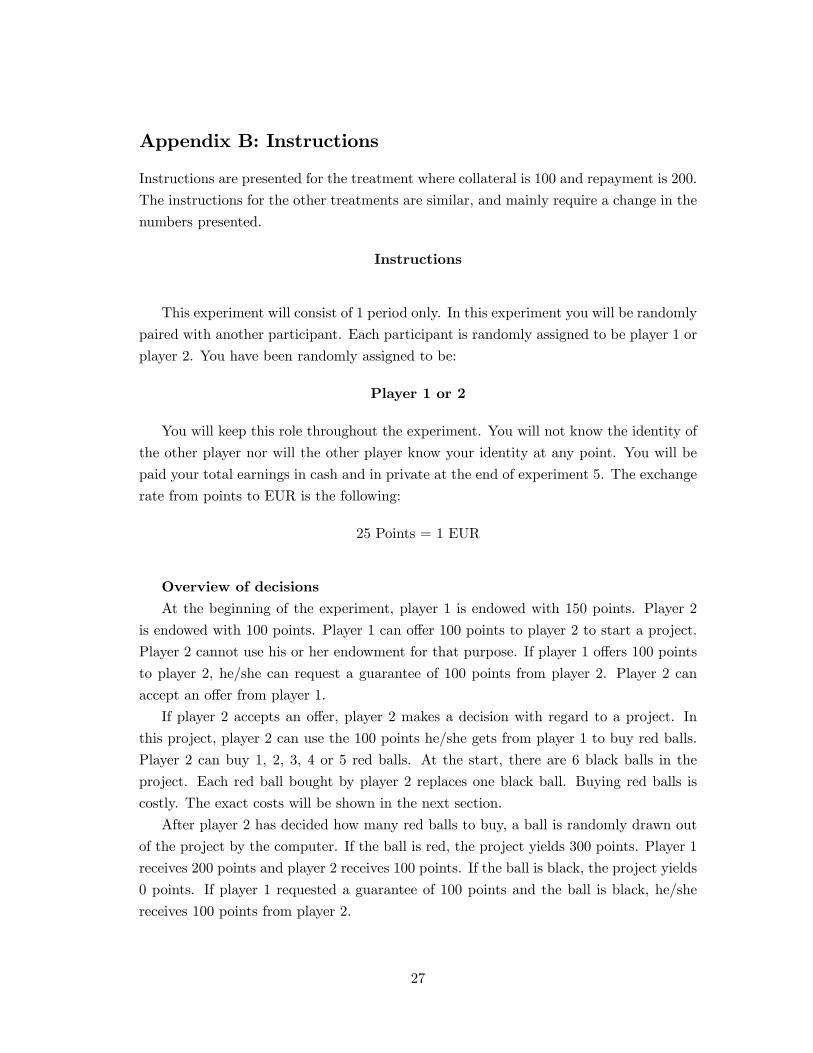
Appendix B: Instructions

Instructions are presented for the treatment where collateral is 100 and repayment is 200.

The instructions for the other treatments are similar, and mainly require a change in the

numbers presented.

Instructions

This experiment will consist of 1 period only. In this experiment you will be randomly

paired with another participant. Each participant is randomly assigned to be player 1 or

player 2. You have been randomly assigned to be:

Player 1 or 2

You will keep this role throughout the experiment. You will not know the identity of

the other player nor will the other player know your identity at any point. You will be

paid your total earnings in cash and in private at the end of experiment 5. The exchange

rate from points to EUR is the following:

25 Points = 1 EUR

Overview of decisionsAt the beginning of the experiment, player 1 is endowed with 150 points. Player 2

is endowed with 100 points. Player 1 can offer 100 points to player 2 to start a project.

Player 2 cannot use his or her endowment for that purpose. If player 1 offers 100 points

to player 2, he/she can request a guarantee of 100 points from player 2. Player 2 can

accept an offer from player 1.

If player 2 accepts an offer, player 2 makes a decision with regard to a project. In

this project, player 2 can use the 100 points he/she gets from player 1 to buy red balls.

Player 2 can buy 1, 2, 3, 4 or 5 red balls. At the start, there are 6 black balls in the

project. Each red ball bought by player 2 replaces one black ball. Buying red balls is

costly. The exact costs will be shown in the next section.

After player 2 has decided how many red balls to buy, a ball is randomly drawn out

of the project by the computer. If the ball is red, the project yields 300 points. Player 1

receives 200 points and player 2 receives 100 points. If the ball is black, the project yields

0 points. If player 1 requested a guarantee of 100 points and the ball is black, he/she

receives 100 points from player 2.

27

Instructions for player 1

Offering pointsAt the beginning of the experiment, you are endowed with 150 points. Player 2 is

endowed with 100 points. You can offer 100 points to player 2 to start a project. Player

2 cannot use his or her endowment for that purpose. If you offer 100 points to player 2,

you can request a guarantee of 100 points from player 2.

In the screenshots attached at the end of the instructions you find an image of the

decision screens you will see during the experiment.These screens are titled ‘Offer screen’.

Accepting offers and buying red ballsPlayer 2 decides whether to accept an offer from you. If player 2 accepts, he/she

can use the 100 points received from you to buy red balls for a project. The more red

balls are bought, the less black balls there are in the project, as displayed in Table 1.

Therefore, the more red balls are bought, the higher is the probability that a red ball is

randomly drawn out of the project.

Number of red balls bought 1 2 3 4 5

The project contains:Number of red balls 1 2 3 4 5

Number of black balls 5 4 3 2 1

Probability that red ball is drawn 1/6 2/6 3/6 4/6 5/6

or 16.7% or 33.3% or 50% or 66.7% or 83.3%Table 1: The project’s red and black balls

Buying red balls is costly for player 2. The exact costs are detailed in Table 2.


Cost 4 16 36 64 100Table 2: Cost of buying red balls

Player 2 will be asked to decide whether he/she accepts your offer and how many red

balls to buy for two cases: if you request no guarantee and if you request a guarantee of

100 points.

At the end of experiment 5, player 2 will be informed about your offer and whether

you requested a guarantee of 100 points. You will be informed about whether player 2

accepted this offer and the color of the ball drawn from the project. You will not be

informed about the number of balls bought by player 2.

28


decision screens player 2 will see during the experiment. These screens are titled ‘Accept

screen’and ‘Project screen’.

PayoffsYour payoffdepends on whether you offer 100 points, whether you request a guarantee

of 100 points, whether player 2 accepts the offer, the number of red balls bought by player

2 and the color of the ball that is thereafter drawn from the project.

If you do not offer 100 points or player 2 does not accept the offer, payoffs are equal

to the initial endowments:

Your payoff = 150

Player 2’s payoff = 100

If you offer 100 points and player 2 accepts this offer, the payoffs depend on whether

the ball drawn from the project is red or black. If the ball drawn is red, your payoff

is equal your endowment, 150 points, minus 100 points offered to player 2, plus the

return you receive from the project, 200 points. Player 2’s payoff is his/her endowment,

100 points, plus 100 points received from you, plus the return he/she receives from the

project, 100 points, and minus the costs of buying red balls.

Your payoff = 150 —100 +200 = 250

Player 2’s payoff = 100 + 100 + 100 —Costs

If the ball drawn is black, your payoff is equal to your endowment, 150 points, minus

100 points offered to player 2, plus the guarantee requested by you. If you did not

request a guarantee, the guarantee requested is 0. If you requested a guarantee, the

guarantee requested is 100 points. Player 2’s payoff is his/her endowment, 100 points,

plus 100 points received from you, minus the costs of buying red balls minus the guarantee

requested by you.

Your payoff = 150 —100 + Guarantee requested

Player 2’s payoff = 100 + 100 —Costs —Guarantee requested

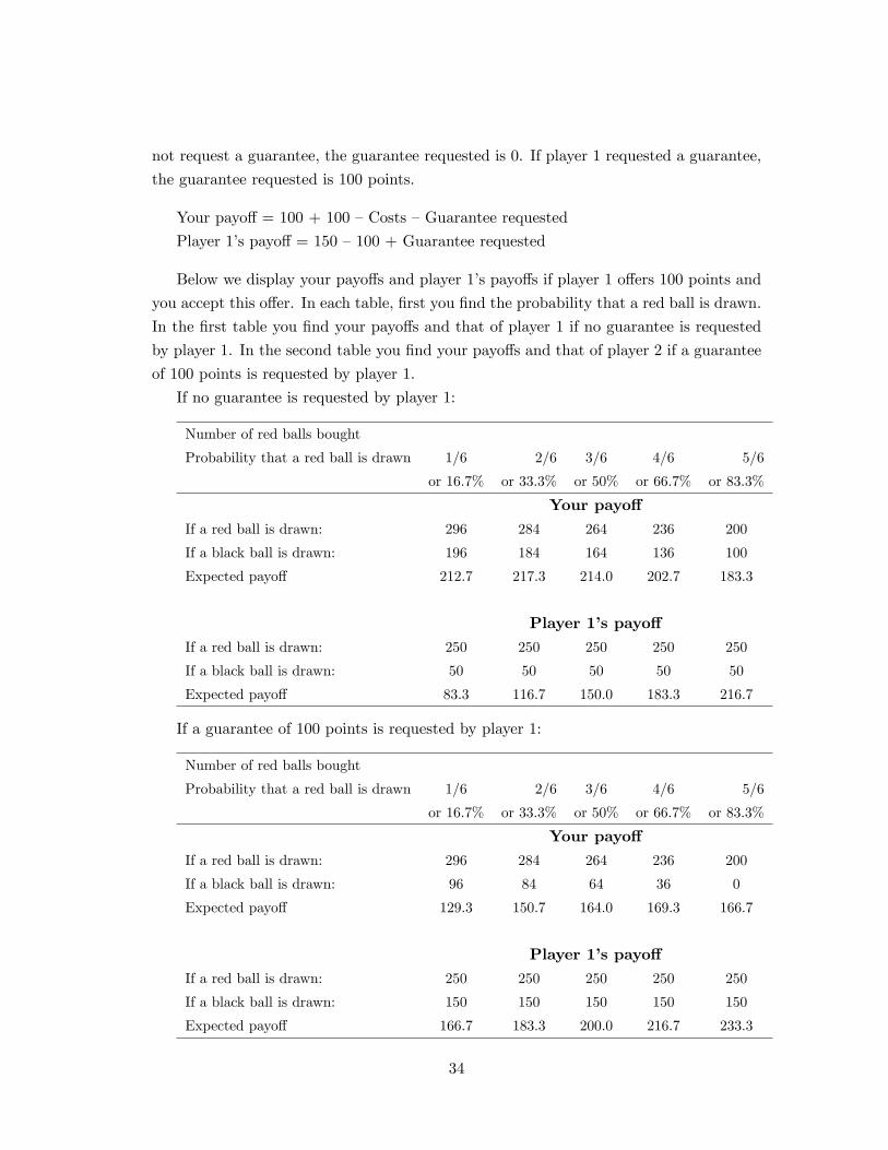
Below we display your payoffs and player 2’s payoffs if you offer 100 points and player

2 accepts this offer. In each table, first you find the probability that a red ball is drawn.

In the first table you find your payoffs and that of player 2 if no guarantee is requested

by you. In the second table you find your payoffs and that of player 2 if a guarantee of

100 points is requested by you.

29

If no guarantee is requested by you:Number of red balls bought

Probability that a red ball is drawn 1/6 2/6 3/6 4/6 5/6

or 16.7% or 33.3% or 50% or 66.7% or 83.3%

Your payoffIf a red ball is drawn: 250 250 250 250 250

If a black ball is drawn: 50 50 50 50 50

Expected payoff 83.3 116.7 150.0 183.3 216.7

Player 2’s payoffIf a red ball is drawn: 296 284 264 236 200


Expected payoff 212.7 217.3 214.0 202.7 183.3

If a guarantee of 100 points is requested by you:Number of red balls bought


or 16.7% or 33.3% or 50% or 66.7% or 83.3%



Expected payoff 166.7 183.3 200.0 216.7 233.3



Expected payoff 129.3 150.7 164.0 169.3 166.7

Beside each computer terminal, you can find a calculator. You may use it to do any

further calculations.

Before the experiment starts, we would like to ask you some questions about the

experiment. Please fill in your answer. If you have finished filling in the questions, please

raise your hand and an experimenter will come to where you are seated. If you have any

questions, please raise your hand.

QuestionsQuestion 1

You do not offer 100 points. What is your payoff and that of player 2?

30

Your payoff =_ _ _ _ _ _ _ _ _ _

Payoff of player 2 =_ _ _ _ _ _ _ _ _ _

Question 2

You offer 100 points and request a guarantee of 100 points. Player 2 does not accept

this offer. What is your payoff and that of player 2?

Your payoff =_ _ _ _ _ _ _ _ _ _

Payoff of player 2 =_ _ _ _ _ _ _ _ _ _

Question 3

You make an offer of 100 points. Player 2 accepts this offer. Please fill in the table

below.

If you do not request a guarantee of 100 points:

Your payoff Player 2’s payoff Probability that red

ball is drawn

If number of red

balls bought is:

1 If red ball is drawn

If black ball is drawn





If you request a guarantee of 100 points:


ball is drawn

If number of red

balls bought is:







SummaryBefore we start, let us briefly summarize the experiment.

31

1. Player 1 decides whether to offer 100 points to player 2 for a project. If he/she

offers 100 points, he/she can request a guarantee of 100 points.

2. Player 2 decides whether to accept this offer.

3. Player 2 decides how many red balls to buy.

4. A ball is randomly drawn from the project.

5. Payoffs are calculated and shown on the screens after Experiment 5.

Instructions for player 2

Offering pointsAt the beginning of the experiment, player 1 is endowed with 150 points. You are

endowed with 100 points. Player 1 can offer 100 points to you to start a project. You

cannot use your endowment for that purpose. If player 1 offers 100 points to you, player

1 can request a guarantee of 100 points from you.


decision screens player 1 will see during the experiment. These screens are titled ‘Offer

screen’.

Accepting offers and buying red ballsYou decide whether to accept an offer from player 1. If you accept, you can use the

100 points received from player 1 to buy red balls for a project. The more red balls are

bought, the less black balls there are in the project, as displayed in Table 1. Therefore,

the more red balls are bought, the higher is the probability that a red ball is randomly

drawn out of the project.


The project contains:Number of red balls 1 2 3 4 5

Number of black balls 5 4 3 2 1

Probability that red ball is drawn 1/6 2/6 3/6 4/6 5/6

or 16.7% or 33.3% or 50% or 66.7% or 83.3%Table 1: The project’s red and black balls

Buying red balls is costly for player 2. The exact costs are detailed in Table 2.

32


Cost 4 16 36 64 100Table 2: Cost of buying red balls

You will be asked to decide whether you accept player 1’s offer and how many red

balls to buy for two cases: if player 1 requests no guarantee and if player 1 requests a

guarantee of 100 points.

At the end of experiment 5, you will be informed about player 1’s offer and whether

player 1 requested a guarantee of 100 points. Player 1 will be informed about whether

you accepted this offer and the color of the ball drawn from the project. Player 1 will

not be informed about the number of balls bought by you.


decision screens you will see during the experiment. These screens are titled ‘Accept

screen’and ‘Project screen’.

PayoffsYour payoff depends on whether player 1 offers 100 points, whether player 1 requests

a guarantee of 100 points, whether you accept the offer, the number of red balls bought

by you and the color of the ball that is thereafter drawn from the project.

If player 1 does not offer 100 points or you do not accept the offer, payoffs are equal

to the initial endowments:

Your payoff = 100

Player 1’s payoff = 150

If player 1 offers 100 points and you accept this offer, the payoffs depend on whether

the ball drawn from the project is red or black. If the ball drawn is red, your payoff is

your endowment, 100 points, plus 100 points received from player 1, plus the return you

receive from the project, 100 points, and minus the costs of buying red balls. Player 1’s

payoff is equal his/her endowment, 150 points, minus 100 points offered to you, plus the

return player 1 receives from the project, 200 points.

Your payoff = 100 + 100 + 100 —Costs

Player 1’s payoff = 150 —100 + 200 = 250

If the ball drawn is black, your payoff is your endowment, 100 points, plus the 100

points received from player 1, minus the costs of buying red balls minus the guarantee

requested by player 1. Player 1’s payoff is equal to player 1’s endowment, 150 points,

minus 100 points offered to you, plus the guarantee requested by player 1. If player 1 did

33

not request a guarantee, the guarantee requested is 0. If player 1 requested a guarantee,

the guarantee requested is 100 points.

Your payoff = 100 + 100 —Costs —Guarantee requested

Player 1’s payoff = 150 —100 + Guarantee requested

Below we display your payoffs and player 1’s payoffs if player 1 offers 100 points and

you accept this offer. In each table, first you find the probability that a red ball is drawn.

In the first table you find your payoffs and that of player 1 if no guarantee is requested

by player 1. In the second table you find your payoffs and that of player 2 if a guarantee

of 100 points is requested by player 1.

If no guarantee is requested by player 1:

Number of red balls bought


or 16.7% or 33.3% or 50% or 66.7% or 83.3%



Expected payoff 212.7 217.3 214.0 202.7 183.3



Expected payoff 83.3 116.7 150.0 183.3 216.7

If a guarantee of 100 points is requested by player 1:

Number of red balls bought


or 16.7% or 33.3% or 50% or 66.7% or 83.3%



Expected payoff 129.3 150.7 164.0 169.3 166.7



Expected payoff 166.7 183.3 200.0 216.7 233.3

34

Beside each computer terminal, you can find a calculator. You may use it to do any

further calculations.

Before the experiment starts, we would like to ask you some questions about the

experiment. Please fill in your answer. If you have finished filling in the questions, please

raise your hand and an experimenter will come to where you are seated. If you have any

questions, please raise your hand.

QuestionsQuestion 1

Player 1 does not offer 100 points. What is your payoff and that of player 1?

Your payoff =_ _ _ _ _ _ _ _ _ _

Payoff of player 1 =_ _ _ _ _ _ _ _ _ _

Question 2

Player 1 offers 100 points and requests a guarantee of 100 points. You do not accept

this offer. What is your payoff and that of player 1?

Your payoff =_ _ _ _ _ _ _ _ _ _

Payoff of player 1 =_ _ _ _ _ _ _ _ _ _

Question 3

Player 1 makes an offer of 100 points. You accept this offer. Please fill in the table

below.

If player 1 does not request a guarantee of 100 points:


ball is drawn

If number of red

balls bought is:







If player 1 requests a guarantee of 100 points:

35


ball is drawn

If number of red

balls bought is:







SummaryBefore we start, let us briefly summarize the experiment.

1. Player 1 decides whether to offer 100 points to player 2 for a project. If he/she

offers 100 points, he/she can request a guarantee of 100 points.

2. Player 2 decides whether to accept this offer.

3. Player 2 decides how many red balls to buy.

4. A ball is randomly drawn from the project.

5. Payoffs are calculated and shown on the screens after Experiment 5.

36

Appendix C: Additional Experimental Data

C.1. Pre-experimental games

The first pre-experimental game was a risk preference elicitation task. Risk preferences

were elicited to have a measure of each subject’s risk aversion, as choosing effort is a

risky choice. The elicitation is similar to that in Heinemann et al (2009) and Dohmen et

al (2010). Each subject is asked to make eleven choices, between a secure payment and a

lottery. While the lottery payout remains constant, 25 points in expectation, the secure

payment increases from 0 to 50 in steps of 5. As the secure payment increases, subjects

are expected to switch from the lottery to the secure payment. If a subject switches to

the secure payment when it is 20 or less, he is classified as risk averse. If he switches

when it is 25, he is classified as risk neutral and risk seeking for the remaining cases. The

variable Risk aversion is thus a dummy variable that takes value one if the subject is

risk averse.12

After the risk elicitation task, subjects played the p−beauty contest game with p = 23

in groups of four. In this game each player chooses a number between 0 and 100. The

winner is the subject whose guess is closest to 2/3 of the average guess (Nagel, 1995). I

measure Strategic reasoning as the difference between 100 and the subject’s guess. Since

the winner is that who is closest to 2/3 of the average, there is a constant unraveling to

lower guesses (until the Nash Equilibrium guess of 0). Thus, a larger difference between

100 and the guess proxies higher levels of strategic reasoning.

Then subjects played a trust game (Berg et al, 1995). In the trust game two players,

A and B, start with 10 points each. Player A can decide how many points (in integers)

to send to player B. The points sent are multiplied by 3 by the experimenter and player

B can freely choose how many to send back to A. For this game, the strategy-method

was used and thus each player played the role of A, deciding how many points to send,

and that of B, deciding for each possible amount sent by A, how many points he or she

would send back. As player B has an incentive to send back 0 points to player A, the

average amount of points sent back by B is used as a proxy for Trustworthiness. The

number of points sent by player A are a measure of trust.13

Table C.1. below presents summary statistics for the variables measured in the pre-

experimental games. While trust and trustworthiness are not significantly different across

treatments, risk aversion and strategic reasoning vary across treatments. For this reason,

these variables are included as controls in the analysis of results.

12Multiple switches are rare: Only 7.8% of the subjects switch multiple times. These subjects areincluded in the data analysis below. Results remain the same if they are excluded.13 In Appendix C.1 the descriptive statistics for these variables are displayed.

37

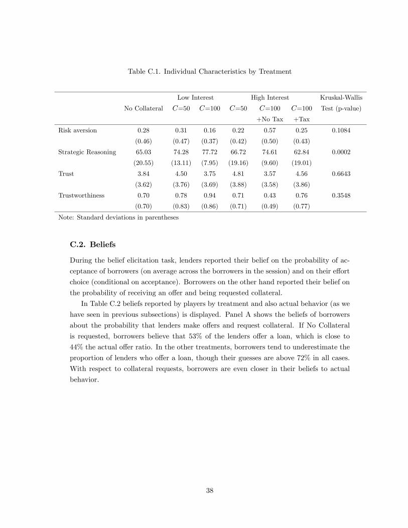
Table C.1. Individual Characteristics by Treatment

Low Interest High Interest Kruskal-Wallis

No Collateral C=50 C=100 C=50 C=100 C=100 Test (p-value)

+No Tax +Tax

Risk aversion 0.28 0.31 0.16 0.22 0.57 0.25 0.1084

(0.46) (0.47) (0.37) (0.42) (0.50) (0.43)

Strategic Reasoning 65.03 74.28 77.72 66.72 74.61 62.84 0.0002

(20.55) (13.11) (7.95) (19.16) (9.60) (19.01)

Trust 3.84 4.50 3.75 4.81 3.57 4.56 0.6643

(3.62) (3.76) (3.69) (3.88) (3.58) (3.86)

Trustworthiness 0.70 0.78 0.94 0.71 0.43 0.76 0.3548

(0.70) (0.83) (0.86) (0.71) (0.49) (0.77)

Note: Standard deviations in parentheses

C.2. Beliefs

During the belief elicitation task, lenders reported their belief on the probability of ac-

ceptance of borrowers (on average across the borrowers in the session) and on their effort

choice (conditional on acceptance). Borrowers on the other hand reported their belief on

the probability of receiving an offer and being requested collateral.

In Table C.2 beliefs reported by players by treatment and also actual behavior (as we

have seen in previous subsections) is displayed. Panel A shows the beliefs of borrowers

about the probability that lenders make offers and request collateral. If No Collateral

is requested, borrowers believe that 53% of the lenders offer a loan, which is close to

44% the actual offer ratio. In the other treatments, borrowers tend to underestimate the

proportion of lenders who offer a loan, though their guesses are above 72% in all cases.

With respect to collateral requests, borrowers are even closer in their beliefs to actual

behavior.

38

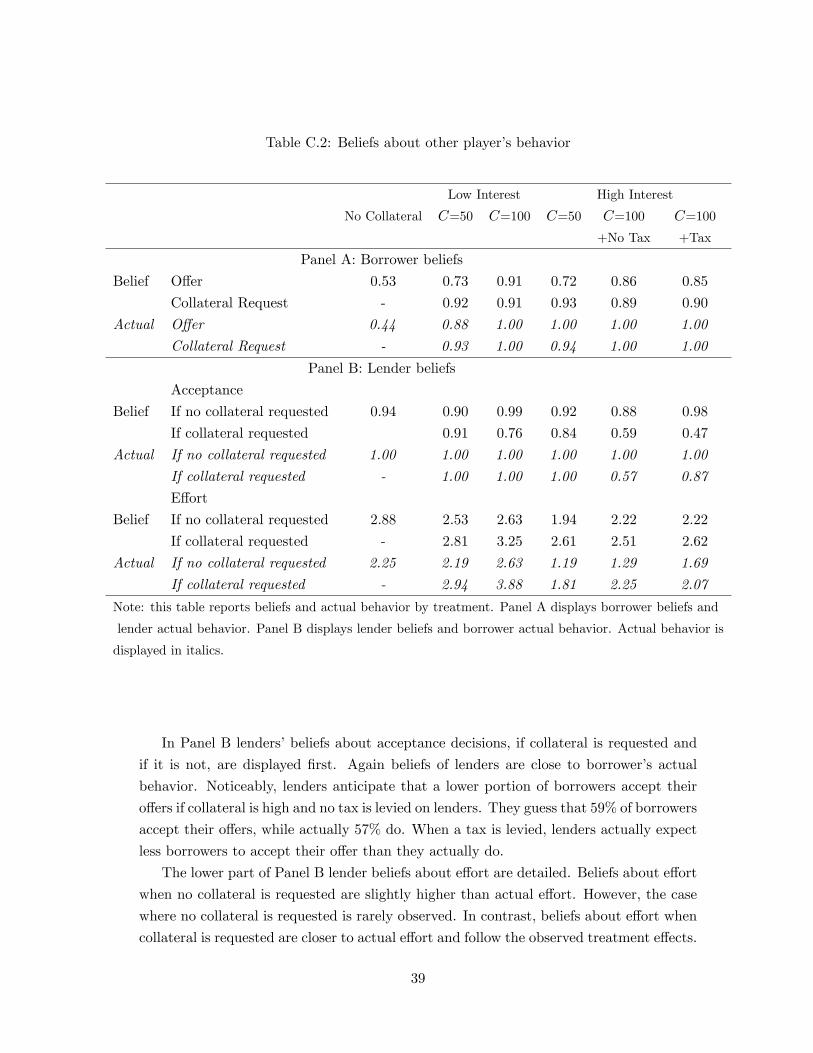
Table C.2: Beliefs about other player’s behavior

Low Interest High Interest

No Collateral C=50 C=100 C=50 C=100 C=100

+No Tax +Tax

Panel A: Borrower beliefs

Belief Offer 0.53 0.73 0.91 0.72 0.86 0.85

Collateral Request - 0.92 0.91 0.93 0.89 0.90

Actual Offer 0.44 0.88 1.00 1.00 1.00 1.00

Collateral Request - 0.93 1.00 0.94 1.00 1.00

Panel B: Lender beliefs

Acceptance

Belief If no collateral requested 0.94 0.90 0.99 0.92 0.88 0.98

If collateral requested 0.91 0.76 0.84 0.59 0.47

Actual If no collateral requested 1.00 1.00 1.00 1.00 1.00 1.00

If collateral requested - 1.00 1.00 1.00 0.57 0.87

Effort

Belief If no collateral requested 2.88 2.53 2.63 1.94 2.22 2.22


Actual If no collateral requested 2.25 2.19 2.63 1.19 1.29 1.69


Note: this table reports beliefs and actual behavior by treatment. Panel A displays borrower beliefs and

lender actual behavior. Panel B displays lender beliefs and borrower actual behavior. Actual behavior is

displayed in italics.

In Panel B lenders’beliefs about acceptance decisions, if collateral is requested and

if it is not, are displayed first. Again beliefs of lenders are close to borrower’s actual

behavior. Noticeably, lenders anticipate that a lower portion of borrowers accept their

offers if collateral is high and no tax is levied on lenders. They guess that 59% of borrowers

accept their offers, while actually 57% do. When a tax is levied, lenders actually expect

less borrowers to accept their offer than they actually do.

The lower part of Panel B lender beliefs about effort are detailed. Beliefs about effort

when no collateral is requested are slightly higher than actual effort. However, the case

where no collateral is requested is rarely observed. In contrast, beliefs about effort when

collateral is requested are closer to actual effort and follow the observed treatment effects.

39

References

[1] Aghion, P. and Bolton, P., 1997. A Theory of Trickle-Down Growth and Develop-

ment, Review of Economic Studies 64, 151-172.

[2] Andreoni, J., 2005. Trust, Reciprocity, and Contract Enforcement: Experiments on

Satisfaction Guaranteed, mimeo.

[3] Banerjee, A.V. and Newman, A.F., 1993. Occupational Choice and the Process of

Development, The Journal of Political Economy 101 (2), 274-298.

[4] Berg,J., Dickhaut, J. and McCabe, K., 1995. Trust, Reciprocity and Social History.

Games and Economic Behavior 10, 122-142.

[5] Berger, Allen N. and Gregory F. Udell, 1990. Collateral, Loan Quality, and Bank

Risk, Journal of Monetary Economics, 25, 21-42.

[6] Berger, A.N., Espinosa-Vega, M.A., Frame, W.S. and Miller, N. H., 2010. Why

do borrowers pledge collateral? New empirical evidence on the role of asymmetric

information. Journal of Financial Intermediation in press.

[7] Berger, A.N., Frame, W.S., and Ioannidou, V., forthcoming. Tests of Ex Ante versus

Ex Post Theories of Collateral using Private and Public Information, Journal of

Financial Economics.

[8] Besley, T. and Ghatak, M., 2009a. The de Soto Effect, CEPR Discussion Paper

7259.

[9] Besley, T. and Ghatak, M., 2009b. Property Rights and Economic Development,

forthcoming in Volume V of the Handbook of Development Economics edited by

Dani Rodrik and Mark Rosenzweig.

[10] Bester, H., 1985. Screening vs. Rationing in Credit Markets with Imperfect Infor-

mation. American Economic Review 75, 850-855

[11] Bester, H., 1987. The Role of Collateral in Credit Markets with Imperfect Informa-

tion. European Economic Review 31, 887-899.

[12] Booij, A. and van de Kuilen, G., 2009. A parameter-free analysis of the utility

of money for the general population under prospect theory, Journal of Economic

Psychology 30, 651—666.

40

[13] Boot, A.W.A., Thakor, A.V. and Udell, G.F., 1991. Secured Lending and Default

Risk: Equilibrium Analysis, Policy Implications and Empirical Results. Economic

Journal 101, 458-472.

[14] Boot, A.W.A. and Thakor, A.V., 1994. Moral Hazard and Secured Lending in an

Infinitely Repeated Credit Market Game, International Economic Review 35(4),

899-920.

[15] Bottazzi, L., Da Rin, M. and Hellmann, T., 2010. The Importance of Trust for

Investment: Evidence from Venture Capital. CentER Discussion Paper Series No.

2010-49, available at SSRN: http://ssrn.com/abstract=997934.

[16] Brown, M., and Zehnder, C., 2007. Credit Reporting, Relationship Banking, and

Loan Repayment, Journal of Money, Credit and Banking 39 (8), 1883-1918.

[17] Brown, M., and Zehnder, C., 2010. The emergence of information sharing in credit

markets, Journal of Financial Intermediation 19, 255—278.

[18] Carter, M. and Olinto, P., 2003. Getting Institutions Right for Whom? Credit

Constraints and the Impact of Property Rights on the Quantity and Composition

of Investment. American Journal of Agricultural Economics 85, 173-86.

[19] Chan, Y. and Thakor, A.V., 1987. Collateral and Competitive Equilibria with Moral

Hazard and Private Information, Journal of Finance 42 (2), 345-363.

[20] Chavis, L. W., Klapper, L.F. and Love, I., 2010. The Impact of the Business En-

vironment on Young Firm Financing. World Bank Policy Research Working Paper

5322.

[21] De Soto, H., 2001. The Mystery of Capital : why capitalism triumphs in the West

and fails everywhere else. Basic Books, New York.

[22] Dohmen, T., Falk, A., Huffman, D., and Sunde, U., 2010. Are Risk Aversion and

Impatience Related to Cognitive Ability? American Economic Review, 100 (3),

1238—1260.

[23] Feder, G., Onchan, T., Chalamwong, Y. and Hongladarom, C., 1988. Land Policies

and Farm Productivity in Thailand. Baltimore: Johns Hopkins Univ. Press (for

World Bank).

[24] Fehr, E. and Schmidt, K., 1999. A Theory of Fairness, Competition and Co-

operation, Quarterly Journal of Economics 114, 817-868.

41

[25] Fehr, E. and Zehnder, K., 2009. Reputation and Credit Market Formation:How

Relational Incentives and Legal Contract Enforcement Interact, IZA DP No. 4351.

[26] Field, E., and Torero, M., 2006. Do Property Titles Increase Credit Access Among

the Urban Poor? Evidence from a Nationwide Titling Program, Working Paper,

Harvard University.

[27] Fischbacher, U., 2007. z-Tree: Zurich Toolbox for Readymade Economic Experi-

ments, Experimental Economics 10, 171-178.

[28] Galiani, S., and Schargrodsky, E., 2010, Property Rights for the Poor: Effects of

Land Titling, Journal of Public Economics, in press.

[29] Heinemann, F., Nagel, R., and Oeckenfels, P., 2009. Measuring Strategic Uncertainty

in Coordination Games, Review of Economic Studies 76, 181—221.

[30] Holmstrom, B. and Tirole, J. 1997. Financial Intermediation, Loanable Funds and

the Real Sector, Quarterly Journal of Economics CXII (3), 663-691.

[31] Innes, R.D., 1990. Limited Liability and Incentive Contracting with Ex-Ante Action

Choices, Journal of Economic Theory 52, 45-67.

[32] Jiménez, G. and Saurina, J., 2004. Collateral, type of lender and relationship banking

as determinants of credit risk, Journal of Banking & Finance 28 (9), 2191-2212.

[33] Jiménez, G., Salas, V. and Saurina, J., 2006. Determinants of collateral. Journal of

Financial Economics 81, 255—281

[34] Kahneman, D. and Tversky, A., 1979. Prospect Theory: An Analysis of Decision

under Risk, Econometrica 47 (2), 263-292.

[35] Levine, D.K., 1998. Modeling Altruism and Spitefulness in Experiments. Review of

Economic Dynamics 1, 593-622.

[36] Levine, R., 2005. Finance and Growth: Theory and Evidence, Handbook of Economic

Growth, Chapter 12, Volume I.A. Edited by Philippe Aghion and Steven N. Durlauf.

[37] Liberti, J. and Mian, A., 2009. Collateral Spread and Financial Development, Jour-

nal of Finance, forthcoming.

[38] Mookherjee, D. and Ray, D., 2002. Contractual Structure and Wealth Accumulation,

American Economic Review 92 (4), 818-849.

42

[39] Nagel, R., 2005. Unraveling in Guessing Games: An Experimental Study, American

Economic Review 85, 1313-1326.

[40] Prelec, D., 1998. The Probability Weighting Function, Econometrica 66, 497-527.

[41] Stiglitz, J.E. and Weiss, A., 1981. Credit Rationing in Markets with Imperfect In-

formation, American Economic Review 71 (3), 393-410.

[42] Townsend, R.M., 1979. Optimal contracts and competitive markets with costly state

verification. Journal of Economic Theory 22, 265—293.

[43] Woodruff, C., 2001. Review of de Soto’s The Mystery of Capital. Journal of Eco-

nomic Literature XXXIX, 1215-1223.

43

moral hazard in credit markets: the incentive e⁄ect of ... · moral hazard in credit markets: the...

Documents