Economic Research Center Middle East Technical University Ankara 06800 Turkey www.erc.metu.edu.tr

ERC Working Papers in Economics 13/02 February / 2013

Financial Crises, Financialization of Commodity

Markets and Correlation of Agricultural Commodity

Index with Precious Metal Index and S&P500

M. Fatih Öztek Department of Economics, Middle East Technical University,

06800, Ankara, TURKEY E-mail: oztek@metu.edu.tr Phone: +(90) 312 210 3041

Nadir Öcal Department of Economics, Middle East Technical University,

06800, Ankara, TURKEY E-mail: ocal@metu.edu.tr

Phone: +(90) 312 210 2071 Fax: +(90) 312 210 7964

2

First draft --- Please do not cite or quote without the permission of authors

Financial Crises, Financialization of Commodity Markets and Correlation of

Agricultural Commodity Index with Precious Metal Index and S&P500

M. Fatih Öztek

a1 Nadir Öcal

a,2

aDepartment of Economics, Middle East Technical University, Ankara, Turkey

Abstract

This paper tests and models time varying correlations among agricultural commodity,

precious metal and S&P500 indices to uncover whether rising trend among these markets

is a result of financialization of commodity markets and/or financial crisis. We

particularly investigate the roles of market news, global and market volatility on the

nature and dynamics of the correlation. Empirical results show that high volatility during

financial crisis is the main source of high correlation of agricultural commodity index

with S&P500 and precious metal index, and plays crucial role in correlation between

precious metal index and S&P500, possibly due to increasing engagement of financial

market investors in commodity markets during financial crisis. Hence, heterogeneous

structure of commodity markets delivers better portfolio diversification opportunities

during calm periods compared to turmoil periods of financial crisis.

JEL Classification: C32, C58, F36, G15

Keywords: Multivariate GARCH, Smooth Transition Conditional Correlation, Portfolio

Diversification, Financialization of Commodity Markets, Index Investment and Equity-

Commodity Co-movements.

1 E-mail: oztek@metu.edu.tr

2 Correspondence to: Prof. Nadir Öcal, Department of Economics, Middle East Technical University, 06800 Ankara,

Turkey; e-mail: ocal@metu.edu.tr

3

1. Introduction

There has been enormous rise in the volume of commodity investment since 2000 mainly due to the

growing interest of financial investors who are recognized as non-commercial participants by Commodity

Futures Trading Commission (CFTC). At the end of 2010, their number was three times higher than the

number of traditional investors engaging in commodity markets to hedge against commodity price

fluctuations (CFTC, 2011). In order to take the advantage of low correlation3 of commodity markets with

financial markets and competitive return rates of commodities, financial investors have intensified

investment in commodities and included investable commodity indices in their portfolios with the

incentive to reduce the risk burden via portfolio diversification. Thus, as an alternative to financial

markets, investable commodity indices such as Standard & Poor’s Goldman Sachs Commodity Index

(S&P-GSCI) or the Dow Jones American International Group Commodity Index (DJ-AIG) or sub-index

of these two indices have emerged as an important class of investment instruments. It is estimated that

total investment in various commodity indices increased from $15 billion in 2003 to $200 billion in 2008

(CFTC, 2008) and to $376 billion at the end of 2010 (Barclays Capital, 2011).

Since the mid-2000s, the increasing role of financial investors in the commodity markets, which give rise

to the term of “financialization of the commodity markets”, has led to the expectation of upward trend in

the correlations of commodity markets with stock markets, as well as with each other. However,

increasing trend in return correlations between commodity and stock markets has not been revealed until

2010. For example, Büyükşahin et al. (2008) use dynamic correlation and recursive co-integration models

but cannot find evidence of increasing trend in the correlations between investable commodity indices

(S&P-GSCI and DJ-AIG, and their sub-indices) and stock market index, S&P500 for the period from

January 1991 to May 2008. They also report that there is no evidence of increase in correlation even

during periods of extreme returns. On the other hand, Silvennoinen and Thorp (2010) manage to find

evidence of increasing trend in the correlations among commodity indices and stock markets in the US,

UK, Germany and France. They model time varying correlation with smooth transition specifications for

the period from May 1990 to July 2009 and show that the return correlations of agricultural commodities

and precious metals (except gold) start to increase between the years 2004 and 2007, and reach to around

0.5. Similarly, Tang and Xiong (2012) document that the return correlation between S&P-GSCI and

S&P500 significantly increases in September 2008 which coincides with financial crisis in the US.

Büyükşahin et al. (2011) find similar results for energy sub-indices of S&P-GSCI by modeling

correlations between weekly returns during the period from January 1991 to May 2011 under the DCC-

GARCH framework. Their results indicate that the correlation between S&P-GSCI energy index and

S&P500 is time varying without a particular trend until September 2008, but since then the correlation

exhibits an upward trend and reaches to very high levels unseen in the prior two decades. These findings,

nevertheless, do not clearly answer whether the rising trend is a result of financialization process and/or

financial crisis. Geetesh and Dunsby (2012) focus on this point and report that tests for a structural break

cannot detect an evidence of permanent increase. Their analysis reveals that the correlation between

commodity and stock markets is higher during economic weakness and hence the recent increase is

attributed to the slowdowns in the GDP growth rates.

This paper investigates how the dynamic structures of return correlations are evolved during the

financialization of commodity markets and the roles of financial crisis on the time varying structure of

3 The findings of earlier literature which employ data series up to year 2004 indicate that the correlations among various

commodity and stock market returns are very low (see Greer (2000), Gorton and Rouwenhorst (2006) and Erb and Harvey

(2006). The works of Becker and Finnerty (1994), Georgiev (2001), Hillier et al. (2006) indicate that moderate investment in

commodity markets provides significant reduction in the risk of portfolio which consists of stocks.

4

correlations by presenting a comprehensive and up-to-date analysis of return correlations among

agricultural commodity, precious metal and SP&500 indices. More specifically, the conditional

correlations among investable S&P-GSCI Agricultural Commodity (S&P-AG), Precious Metal (S&P-

PM) sub-indices and S&P500 index are modeled in the context of multivariate generalized autoregressive

conditional heteroscedasticity (MGARCH) with time varying conditional correlations. We prefer smooth

transition conditional correlation (STCC-GARCH) and double smooth transition conditional correlation

(DSTCC-GARCH) specifications proposed by Silvennoinen and Teräsvirta (2005 and 2009). By using

calendar time as a transition variable in STCC-GARCH model, the first aim is to search for evidence of

increasing trend in the conditional correlation which is expected as a natural result of financialization

process. To examine the effects of financial crisis on correlations, secondly, we investigate the roles of

market conditions represented by global volatility, index specific volatility and the news from the indices

whose effects on the dynamic nature of conditional correlation is of interest in terms of portfolio

diversification for a long time in the literature. Various measures of these factors are employed as

candidate transition variables in the context of STCC-GARCH and DSTCC-GARCH models. The results

imply that the increasing trend hypothesis is valid for conditional correlation between S&P-PM and

S&P500 but not for S&P-AG – S&P500 and S&P-AG – S&P-PM pairs. The DSTCC-GARCH models

reveal that the volatility of S&P-AG and S&P500 play key role in determining the conditional correlation

between these two indices. Although, our results show increasing correlation during the recent financial

crisis, this not a new phenomenon or specific to recent crisis but commonly observed when both

agricultural commodity and stock markets are in turmoil during financial crisis and correlation may return

back to its low levels if the markets calm down. Similarly, the high conditional correlation levels

between S&P-AG and S&P-PM appear when volatility in S&P-AG and S&P-PM sub-indices is higher

and tends to lower levels following the decline in the volatilities putting doubts on the permanency of

high correlation levels. Generally speaking, our results show that rising trend hypothesis may not be a

result of financial integration between markets but may generally be related to high volatility observed

during financial crisis reflecting the fact that commodity markets are seen as safe harbor during the severe

crisis.

The plan of the paper is as follows. Next section introduces the models and estimation details. Section 3

introduces the data set and presents the estimation results. Final section concludes the paper.

2. Econometric Models and Estimation

Due to its computational simplicity and direct interpretation of model parameters, Dynamic Conditional

Correlation (DCC) specification of Engle (2002) is the most popular model in defining conditional

correlation equation. However we prefer smooth transition conditional correlation (STCC) and double

smooth transition conditional correlation (DSTCC) models of Silvennoinen and Teräsvirta (2005 and

2009) due to their flexibility compared to DCC model. These models define conditional correlation as a

function of observable variable(s) providing high flexibility in terms of variable selection for conditional

correlation equation4. Hence, in line with our aims, these models not only allow us to characterize

increasing trend by using calendar time as a transition variable but also flexible enough to uncover the

4 Besides, (D)STCC-GARCH specifications allow interaction between GARCH process and conditional correlation equations by

simultaneous estimation instead of two-step estimation. By defining smooth transition, these models are capable of incorporating

the possibility of heterogeneous agents which may respond to developments at different values of transition variable. And also in

this framework any structural change through time or with respect to particular transition variable can be detected without ex ante

information of change.

5

structure and properties of the time varying correlation in response to volatility both in global and local

levels and the news from markets.

The relevant equations and modeling procedure can be given as follows. The mean equations of stock

returns for a 2-dimensional stochastic vector of stock returns is

( | ) (1)

[ ] (2)

where Ɵt-1 contains all available information up to time t-1. The conditional covariance of the shocks in

equation (1) are time-varying, such that

| ( ) (3)

Instead of defining Ht directly, by following Bollerslev (1990) it is decomposed as

(4)

where Dt is a 2×2 diagonal matrix whose diagonal elements are square root of conditional variances (i.e.

√ and √ ) and Rt is a symmetric conditional correlation matrix whose diagonal elements are unity

and off-diagonal elements are between -1 and 1. Dynamics for elements of Dt are defined with imposing

the non-negativity and stationarity restrictions and each element can follow different GARCH processes.

Since the performance of GARCH(1,1) model is sufficient to represent many dynamics of financial time

series, each element of Dt, i.e. each variance, is modeled as GARCH(1,1) process separately5. Therefore,

in this way conditional covariance matrix is defined indirectly and its conditional covariance elements are

represented by product of conditional correlation and square root of conditional variances.

(5)

( ) (6)

Under this formulation, variance is time varying as defined in equation (5) and covariances are time

varying due to variation in both variance and correlation by construction.

Silvennoinen and Teräsvirta (2005), in defining Rt, assume that it is governed by two extreme regimes

and the conditional correlation changes smoothly between these regimes,

( ( )) ( ) (7)

where P1 and P2 are regime specific constant correlation matrices whose diagonal entries must be unity

and off-diagonal elements must be less than or equal to unity in absolute value as in regular correlation

matrix. However unlike DCC-GARCH model, this is not guaranteed by construction. The elements of P1

and P2 are parameters to be estimated and need to be controlled during estimation.

5 For S&P-PM, GARCH(3,1) eliminates the dependence in squared standardized errors.

6

In equation (7), Gt (st ; γ,c) is the transition function of an observable transition variable, st, and bounded

between zero and unity. These extremes (Gt = 0 and Gt =1) may be associated with distinct regimes, such

as high and low correlation regimes. When Gt is equal to zero, the conditional correlation is governed by

only P1 and said to be in the first regime. Similarly, when G(.) takes on the value of one, conditional

correlation equals to P2 and in the second regime. Transition period between extreme regimes correspond

to the values of the transition function in between Gt = 0 and Gt =1 in which the conditional correlation,

Rt, is a convex combination of P1 and P2. The proper choice of transition function is the logistic one

( ( )) (8)

Slope parameter γ indicating the smoothness of transition and location (threshold) parameter c showing

the half-way point between two regimes characterize this function which is monotonically increasing

from zero to unity. Which in turn makes Rt a linear combination of P1 and P2 and it describes a monotonic

transition from P1 to P2 as (st - c) increases6. Large values of parameter γ imply sharp transition between

two regimes.

DSTCC-GARCH model is a generalization of Equation (7) to allow for two transition functions with two

distinct transition variables by relaxing the assumption that P1 and P2 are regime specific constant

correlations. Define P1,t and P2,t and reformulate Rt as

( ( )) ( ) (9)

As a function of second transition function with respect to observable second transition variable, P1,t and

P2,t take values between P11 and P12, and P21 and P22 respectively.

( ( )) ( ) (10)

When we substitute equation (10) in to equation (9), the conditional correlation equation becomes

( ) (( ) ) (( ) ) (11)

where the transition functions G1,t (s1,t ; γ1 ,c1) and G2,t (s2,t ; γ2 ,c2) are logistic functions with different

transition variables (s1,t , s2,t), different locations (c1 , c2) and different slope parameters (γ1, γ2). P11, P12,

P21 and P22 are regime specific constant correlation matrices. Two different regimes P1 and P2 are

described by the first transition function and the second one allows two distinct regimes within the each

regime of the former one (P1 → P11 and P12 ; P2 → P21 and P22). Therefore in DSTCC-GARCH model the

conditional correlation, Rt, is governed by four regimes7. When the conditional correlation is in the first

regime with respect to the second transition function (i.e. G2,t = 0) Rt takes on values between P11 and P21

as a function of the first transition function, and during the second regime (when G2,t = 1) it takes on

values between P12 and P22 as a function of the first transition function. Hence, the system can move from

6 A special case of the STCC model uses scaled calendar time as the transition variable, st = t / T, which gives rise to the time-

varying conditional correlations model of Berben and Jansen (2005). This allows one smooth change between correlation regimes

and as γ → ∞ model captures a structural break in the correlations. This transition variable may be particularly relevant in order

to capture the effects of increasing integration of financial markets. 7If the transition variables are the same then conditional correlation is governed by three extreme regime specific correlations

with two distinct transition functions, see Öcal and Osborn (2000).

7

P11 to P21 and P12 to P22 only by the dynamics of the first transition function in case of these extremes.

Otherwise, the movements among four regimes are governed by both transition functions.

Conditional correlation between three index pairs (S&P-AG – S&P500, S&P-PM – S&P500 and S&P-

AG – S&P-PM) are modeled separately, rather than analyzing all indices under one specification for the

following reasons: modeling correlation matrix of a multivariate model with more than two variables in

STCC-GARCH and DSTCC-GARCH framework implicitly impose the condition that the correlation

between all pairs must be governed by not only the same transition variable with same lag, but also by the

same threshold value and same slope parameter. As far as the former concerned, this requires the

assumption that the correlations between, for example, S&P-AG – S&P500 and S&P-AG – S&P-PM are

governed by same transition variable which may not be realistic. Although it is possible to generalize

these models with common transition variable but different slope and threshold parameters, this is quite

impractical due to increasing number of parameters to be estimated and also the positive definiteness of

correlation matrix may be difficult to retain as pointed out in Silvennoinen and Teräsvirta (2005 and

2009). Even if one manages to estimate a multivariate model with several transitions functions, the

interpretation of parameters may not be an easy task and inferences on bivariate dynamics may not be an

easy task. As our results show in section 3.2, different transition variables for different index pairs govern

the change from one correlation regime to other strengthening our view. In addition, transition dates do

not seem to be matching, making a multivariate modeling impractical at least for the indices analyzed

here.

We basically follow the methodology suggested in Silvennoinen and Teräsvirta (2005, 2009) which can

briefly be outlined as follows.

Test the null hypothesis of constant conditional correlation (CCC) against the alternative

hypothesis of STCC-GARCH with alternative transition variables by LM1 test of Silvennoinen

and Teräsvirta (2005). In line with our purposes, four groups of variables are taken in to account;

only calendar time is included in the first group to check the increasing trend hypothesis, the

second group contains VIX index as a measure of global volatility, the third one consists of

variables to measure index specific volatility (lagged conditional variance8, lagged absolute error

and lagged absolute standardized error9, lagged squared error and lagged squared standardized

errors) and the last group consists of measures of the news from indices (lagged errors and lagged

standardized error). To find the appropriate transition variables, all variables in each group and up

to four lags of all variables in the last three groups producing 61 candidate transition variables for

S&P-AG – S&P500 and S&P-PM – S&P500 pairs are considered. For S&P-AG – S&P-PM pair,

variables derived for S&P500 are also taken in to account making 89 transition variable

candidates. If the null hypothesis cannot be rejected, estimation of STCC-GARCH model is not

recommended since the parameters of the correlation equation in the STCC-GARCH

specification are not identified and its estimation may lead to inconsistent parameter estimates.

Estimate STCC-GARCH specification with the transition variable enabling the rejection of the

null hypothesis. However, since the candidate transition variables may carry similar information

about the change in the correlation dynamics, it is highly likely that the null hypothesis can be

rejected for more than one candidate transition variable with close p-values preventing a clear cut

8 Conditional variance series are generated by univariate GARCH(1,1) model for each index separately. 9 Errors are from GARCH(1,1) model and standardized errors are generated by dividing errors to square root of conditional

variance.

8

selection. In this case we prefer to fit STCC-GARCH with each of them and leave the selection of

best model and / or appropriate transition variable to post-estimation.

Conduct LM2 test of Silvennoinen and Teräsvirta (2009) to all estimated STCC-GARCH models

in the first step to uncover whether a second transition function is needed by again considering all

variables in the four groups. This not only help us to identify the second transition function but

also to have an idea if the transition variable used in the estimation of the best STCC-GARCH

model is the optimal one. If the null hypothesis of STCC-GARCH model with the best transition

variable is rejected against the alternative DSTCC-GARCH models for more than one transition

variable, we again estimate DSTCC-GARCH model for all of them and leave model selection to

post estimation.

Estimate STCC-GARCH and DSTCC-GARCH models by maximum likelihood (ML) under the

assumption of conditional normality of standardized errors.

| ( ) (12)

where then the log-likelihood for observation t is

( ) ( )∑ ( ) ( ) | | ( )

(13)

and ∑ is maximized with respect to model parameters.

Nonlinear feature of the model and the large number of parameters make estimation of all equations

(mean, conditional variance and correlation, and transition function) jointly at once quite problematic.

Moreover, initial values of parameters are very crucial in estimation and different initial values may lead

to convergence to different parameter values which may correspond to local maxima. To overcome this

problem to some extent, grid search over the parameters of the transition functions are performed. The

initial values of parameters in mean, conditional variance and correlation equations are determined by

following the iterative procedure suggested by Silvennoinen and Teräsvirta (2005) which divides the

parameters into three sets: parameters in the mean and variance equations, correlations, and parameters of

the transition function, and the log-likelihood is maximized by sequential iteration over each set by

holding the parameters of other set at their previously estimated values. With these initial values, all

equations are estimated simultaneously at once10

.

The estimated models are first assessed for their ability to capture the conditional correlation dynamics

via transition between regime specific constant correlations. At this point, the location of the estimated

threshold value and the estimated correlation levels corresponding to each regime are very important. If

the number of observations, above or below the estimated threshold value is very small and/or the

difference between correlation regimes is insignificant, estimated STCC-GARCH and DSTCC-GARCH

models are discarded. The best model, among the satisfactory ones, is selected according to maximum

likelihood value.

10 All estimations are performed using RATS 8.0. Our own source codes are adapted from the Ox code which is kindly supplied

by Annastiina Silvennoinen.

9

Since the interpretation of individual parameter estimates is not very informative due to large number of

parameters, following the literature we prefer the graphs of estimated conditional correlations to evaluate

the estimation results.

3. Data and Empirical Results

3.1 Data

The weekly return rates of S&P-GSCI Agriculture (S&P-AG) and Precious Metal (S&P-PM) sub-indices,

and S&P500 index denominated in US dollar for the period from January 4, 1990 to December 20, 2012

are used in the estimations. The weekly return rates are calculated by log-differencing Thursday closing

prices11

. The data is obtained from Global Financial Data. The extreme returns which are outside the four

standard deviations confidence interval around the mean are replaced with their boundary values. This

truncation is necessary not only in estimation of GARCH parameters but also to alleviate the effects of

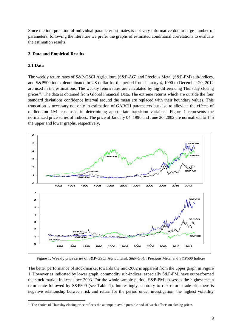
outliers on LM tests used in determining appropriate transition variables. Figure 1 represents the

normalized price series of indices. The price of January 04, 1990 and June 20, 2002 are normalized to 1 in

the upper and lower graphs, respectively.

Figure 1: Weekly price series of S&P-GSCI Agricultural, S&P-GSCI Precious Metal and S&P500 Indices

The better performance of stock market towards the mid-2002 is apparent from the upper graph in Figure

1. However as indicated by lower graph, commodity sub-indices, especially S&P-PM, have outperformed

the stock market indices since 2003. For the whole sample period, S&P-PM possesses the highest mean

return rate followed by S&P500 (see Table 1). Interestingly, contrary to risk-return trade-off, there is

negative relationship between risk and return for the period under investigation; the highest volatility

11 The choice of Thursday closing price reflects the attempt to avoid possible end-of-week effects on closing prices.

10

level corresponds to the lowest mean return (S&P-AG) and the lowest volatility corresponds to the

highest mean return level (S&P-PM). The S&P-AG and S&P500 indices are left skewed a typical feature

common to most of the financial time series. Besides, the fat tail property of financial time series is also

apparent from the excess kurtosis of all indices, hence observing extreme returns are more likely. But the

S&P-PM index is right skewed implying that large negative returns are not as likely as large positive

returns which mean that precious metal index is not more risky in terms of losses either.

Mean SD Skewness Kurtosis (excess)

S&P-AG 0.059 2.639 -0.239 3.155

S&P-PM 0.125 2.352 0.113 5.302

S&P500 0.120 2.357 -1.303 9.982

Table 1: Descriptive statistics of weekly return rates

The unconditional sample correlations among indices are presented in Table 2. The correlation levels are

very low relative to the correlations among international stock market indices and it is almost zero

between precious metal and stock market indices supporting the view that agricultural and precious metal

commodity indices may offer valuable opportunities to reduce risk via portfolio diversification.

S&P-AG S&P-PM S&P500

S&P-AG 1 0.257 0.134

S&P-M 1 0.007

Table 2: Sample correlations of weekly return rates

3.2 Empirical Results

3.2.1. STCC-GARCH Models

We first conduct LM1 test of Silvennoinen and Teräsvirta (2005) to test the null hypothesis of CCC

against alternative of the STCC model with transition variables time, to test increasing trend hypothesis

and all variables in the other three groups, global volatility, index specific volatility and the news from the

indices with their four lags to uncover the role of market conditions in explaining the nature of

correlation12

.

LM1 test results in Table 3 shows that the determinant of time varying conditional correlation between

S&P-AG and S&P500 could be time, global volatility represented by second lag of VIX and volatility

measures of S&P500 and S&P-AG; second lag conditional volatility of S&P500, fourth lag of conditional

volatility of S&P-AG and first lag of squared error of S&P-AG. For S&P-PM and S&P500 pair,

alternative transition variables are time, news from both S&P500 and S&P-PM represented by errors and

standardized errors, and volatility measures of both S&P500 and S&P-PM. Finally, volatility measures of

S&P-AG, S&P-PM and S&P500 seem to be appropriate transition variables for S&P-AG and S&P-PM

pair.

12 In a similar work, Silvennoinen and Thorp (2010) use smooth transition specifications for correlation analysis by considering

alternative transition variables but not as comprehensive as the one considered here as we include various volatility measures of

indices, not to mention the larger sample size covering the aftermath of the recent financial crisis. This cautious approach seems

to be rewarding as empirical results show that volatility in the markets is one of main sources behind high correlation which

seems to be decreasing following declines in the market volatilities.

11

S&P-AG - S&P500 S&P-PM - S&P500

Transition variable LM-Stat p-value Transition variable LM-Stat p-value

Time 13.137a

0.000 Time 15.865a

0.000

vol.AG-L4 11.226a

0.000 err.PM-L2 7.826a

0.005

vol.SP-L2 5.621b

0.018 serr.PM-L2 6.301b

0.012

vix-L2 5.523b

0.019 a[err.PM]-L2 6.020b

0.014

s[err.AG]-L1 4.075b

0.043 s[err.PM]-L2 5.322b

0.021

S&P-AG - S&P-PM vol.PM-L1 5.191b

0.023

a[err.PM]-L3 8.102a

0.004 err.SP-L1 7.427a

0.006

vol.PM-L1 6.479b

0.011 serr.SP-L1 5.523b

0.019

vol.AG-L1 5.328b

0.021 a[err.SP]-L1 7.053a

0.008

s[err.AG]-L3 4.453b

0.035 s[err.SP]-L1 6.251b

0.012

s[err.SP]-L2 4.070b

0.043 a[serr.SP]-L1 7.753a

0.005

s[serr.SP]-L1 9.210a

0.002

Notes: This table reports the LM1 statistic of testing constant conditional correlation null hypothesis with

respect to particular transition variable. The LM1 statistics is evaluated with the estimated parameters from

the restricted model of CCC model (see Silvennoinen and Teräsvirta, 2005). "err", "serr" and “vol” are error,

standardized error and variance from GARCH (1,1) process. S[.] and A[.] represent square and absolute

value of square brackets respectively. "-Li" is ith lag of the particular variable. "AG", "PM" and "SP"

represent S&P-AG, S&P-PM and S&P500 indices. (a) and (b) denote significance at 1% and 5% levels,

respectively.

Table 3: Constant conditional correlation test against STCC-GARCH model with one transition variable

Since the p-values reported in Table 3 are very close to each other, STCC-GARCH models are estimated

with all significant transition variables and the selection of best transition variable is postponed to post-

estimation. The results13

show that for conditional correlations of commodity sub-indices with stock

market index (i.e. S&P-AG and S&P500, and S&P-PM and S&P500) time variable provides the best fit

according to ML values. For correlation between commodity sub-indices (S&P-AG and S&P-PM), the

best model is delivered by volatility measure of precious metal sub-index; first lag of conditional

volatility of S&P-PM. Table 4 presents the estimation results of conditional correlation equation for each

pair which correspond to these best fits.

Transition Variable ML Value P₁ P₂ γ₁ c₁

S&P-AG – S&P500 Time -5109.903 0.003 0.373a 400 0.813

a

(0.033) (0.051) - (0.005)

S&P-PM – S&P500 Time -4910.982 -0.098a

0.165a 400 0.604

a

(0.037) (0.044) - (0.005)

S&P-AG – S&P-PM vol.PM-L1 -5092.603 0.132a

0.365a 400 5.385

a

(0.008) (0.043) - (0.006)

Notes: This Table reports the estimation results of parameters in conditional correlation and transition function

which is described by equations (7) and (8), respectively from the STCC-GARCH model with stated transition

variable. The mean and variance equations are given by (1) and (5), respectively. Values in parenthesis are

standard errors. 400 is the upper constraint for speed parameters. (a) denotes significance at 1% level.

Table 4: The estimation results of STCC-GARCH model with transition variable providing the best fit

13 These results are not reported, but available upon request.

12

It should be mentioned that the rejection of CCC assumption for more than one transition variable by LM1

test may indicate that the estimated STCC-GARCH model with one of them may not be adequate to

capture the dynamic structure of the conditional correlation and puts doubts on the inferences based on

STCC-GARCH model. The model may need a second transition function as in the DSTCC-GARCH

specification to have a better description of the data. Therefore we mainly focus on the results of latter

class of models in the next sections but briefly interpret the STCC-GARCH model with time variable to

see the timing of increase and the average level of correlations attained through time.

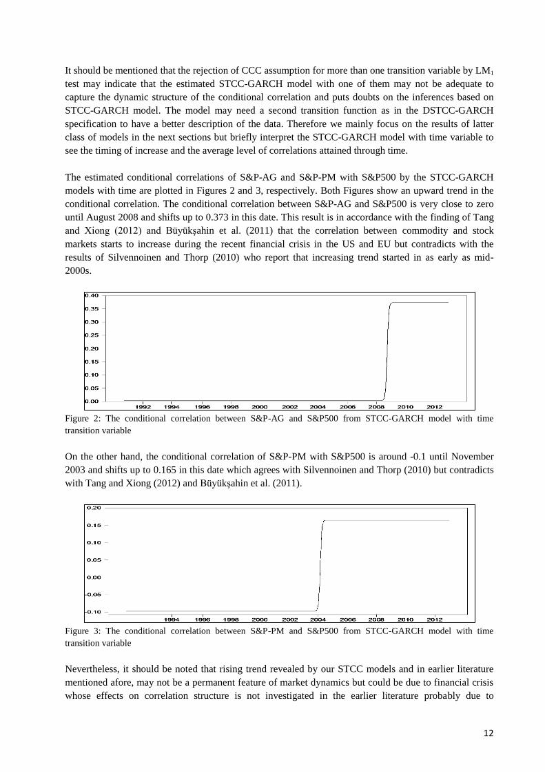
The estimated conditional correlations of S&P-AG and S&P-PM with S&P500 by the STCC-GARCH

models with time are plotted in Figures 2 and 3, respectively. Both Figures show an upward trend in the

conditional correlation. The conditional correlation between S&P-AG and S&P500 is very close to zero

until August 2008 and shifts up to 0.373 in this date. This result is in accordance with the finding of Tang

and Xiong (2012) and Büyükşahin et al. (2011) that the correlation between commodity and stock

markets starts to increase during the recent financial crisis in the US and EU but contradicts with the

results of Silvennoinen and Thorp (2010) who report that increasing trend started in as early as mid-

2000s.

Figure 2: The conditional correlation between S&P-AG and S&P500 from STCC-GARCH model with time

transition variable

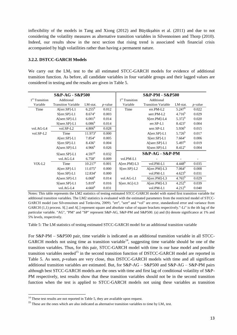
On the other hand, the conditional correlation of S&P-PM with S&P500 is around -0.1 until November

2003 and shifts up to 0.165 in this date which agrees with Silvennoinen and Thorp (2010) but contradicts

with Tang and Xiong (2012) and Büyükşahin et al. (2011).

Figure 3: The conditional correlation between S&P-PM and S&P500 from STCC-GARCH model with time

transition variable

Nevertheless, it should be noted that rising trend revealed by our STCC models and in earlier literature

mentioned afore, may not be a permanent feature of market dynamics but could be due to financial crisis

whose effects on correlation structure is not investigated in the earlier literature probably due to

13

inflexibility of the models in Tang and Xiong (2012) and Büyükşahin et al. (2011) and due to not

considering the volatility measures as alternative transition variables in Silvennoinen and Thorp (2010).

Indeed, our results show in the next section that rising trend is associated with financial crisis

accompanied by high volatilities rather than having a permanent nature.

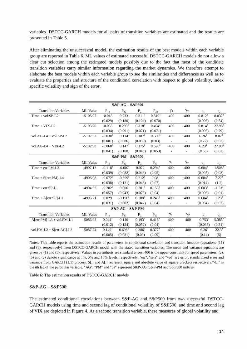
3.2.2. DSTCC-GARCH Models

We carry out the LM2 test to the all estimated STCC-GARCH models for evidence of additional

transition function. As before, all candidate variables in four variable groups and their lagged values are

considered in testing and the results are given in Table 5.

S&P-AG - S&P500 S&P-PM - S&P500 1

st Transition

Variable

Additional

Transition Variable LM-stat. p-value

1st Transition

Variable

Additional

Transition Variable LM-stat. p-value

Time A[err.SP]-L1 6.255b 0.012 Time err.PM-L2 5.247b 0.022

S[err.SP]-L1 8.674a 0.003

serr.PM-L2 4.716b 0.029

A[serr.SP]-L1 6.001b 0.014

S[err.PM]-L4 5.372b 0.020

S[serr.SP]-L1 6.086b 0.014 err.SP-L1 8.423a 0.004

vol.AG-L4 vol.SP-L2 4.806b 0.028 serr.SP-L1 5.936b 0.015

vol.SP-L2 Time 11.973a 0.000 A[err.SP]-L1 5.726b 0.017

A[err.SP]-L1 7.854a 0.005 S[err.SP]-L1 7.664a 0.006

S[err.SP]-L1 8.436a 0.004 A[serr.SP]-L1 5.497b 0.019

A[serr.SP]-L1 4.966b 0.026 S[serr.SP]-L1 8.412a 0.004

S[serr.SP]-L1 4.597b 0.032 S&P-AG - S&P-PM

vol.AG-L4 6.758a 0.009 vol.PM-L1 - - -

VIX-L2 Time 10.217a 0.001 A[err.PM]-L3 vol.PM-L1 4.448b 0.035

A[err.SP]-L1 11.075a 0.000 S[err.SP]-L2 A[err.PM]-L3 7.064a 0.008

S[err.SP]-L1 12.834a 0.000 vol.PM-L1 4.623b 0.031

A[serr.SP]-L1 6.068b 0.014 vol.AG-L1 A[err.PM]-L3 4.765b 0.029

S[serr.SP]-L1 5.819b 0.016 S[err.AG]-L3 A[err.PM]-L3 4.252b 0.039

vol.AG-L4 4.660b 0.031 vol.PM-L1 4.212b 0.040

Notes: This table represents the LM2 statistics of testing estimated STCC-GARCH model with stated first transition variable for

additional transition variables. The LM2 statistics is evaluated with the estimated parameters from the restricted model of STCC-

GARCH model (see Silvennoinen and Teräsvirta, 2009). "err", "serr" and “vol” are error, standardized error and variance from

GARCH (1,1) process. S[.] and A[.] represent square and absolute value of square brackets respectively."-Li" is the ith lag of the

particular variable. "AG", "PM" and "SP" represent S&P-AG, S&P-PM and S&P500. (a) and (b) denote significance at 1% and

5% levels, respectively.

Table 5: The LM statistics of testing estimated STCC-GARCH model for an additional transition variable

For S&P-PM – S&P500 pair, time variable is indicated as an additional transition variable in all STCC-

GARCH models not using time as transition variable14

, suggesting time variable should be one of the

transition variables. Thus, for this pair, STCC-GARCH model with time is our base model and possible

transition variables needed15

in the second transition function of DSTCC-GARCH model are reported in

Table 5. As seen, p-values are very close, thus DSTCC-GARCH models with time and all significant

additional transition variables are estimated. But, for S&P-AG – S&P500 and S&P-AG – S&P-PM pairs

although best STCC-GARCH models are the ones with time and first lag of conditional volatility of S&P-

PM respectively, test results show that these transition variables should not be in the second transition

function when the test is applied to STCC-GARCH models not using these variables as transition

14 These test results are not reported in Table 5, they are available upon request. 15

These are the ones which are also indicated as alternative transition variables to time by LM1 test.

14

variables. DSTCC-GARCH models for all pairs of transition variables are estimated and the results are

presented in Table 5.

After eliminating the unsuccessful model, the estimation results of the best models within each variable

group are reported in Table 6. ML values of estimated successful DSTCC-GARCH models do not allow a

clear cut selection among the estimated models possibly due to the fact that most of the candidate

transition variables carry similar information regarding the market dynamics. We therefore attempt to

elaborate the best models within each variable group to see the similarities and differences as well as to

evaluate the properties and structure of the conditional correlation with respect to global volatility, index

specific volatility and sign of the error.

S&P-AG – S&P500

Transition Variables ML Value P11 P12 P21 P22 γ1 γ2 c1 c2

Time + vol.SP-L2 -5105.97 -0.018 0.233 0.311a 0.519a 400 400 0.812a 8.032a

(0.029) (0.180) (0.104) (0.070) - - (0.006) (2.54)

Time + VIX-L2 -5103.70 -0.033 0.293a 0.318a 0.494a 400 400 0.814a 27.98a

(0.034) (0.091) (0.071) (0.071) - - (0.006) (0.29)

vol.AG-L4 + vol.SP-L2 -5102.52 -0.030a 0.114 0.187a 0.580a 400 400 6.26a 8.02a

(0.001) (0.086) (0.036) (0.03) - - (0.27) (0.52)

vol.AG-L4 + VIX-L2 -5102.93 -0.068c 0.147 0.175a 0.526a 400 400 6.23a 27.99a

(0.041) (0.108) (0.043) (0.053) - - (0.63) (0.82)

S&P-PM – S&P500

Transition Variables ML Value P11 P12 P21 P22 γ1 γ2 c1 c2

Time + err.PM-L2 -4907.13 -0.118a -0.007 0.072 0.294a 400 400 0.604a 1.508a

(0.039) (0.082) (0.048) (0.05) - - (0.005) (0.03)

Time + S[err.PM]-L4 -4906.98 -0.072c -0.399a 0.212a 0.08 400 400 0.604a 7.22a

(0.038) (0.131) (0.048) (0.07) - - (0.014) (1.2)

Time + err.SP-L1 -4904.52 -0.282a 0.006 0.201a 0.153a 400 400 0.603a -1.31a

(0.057) (0.043) (0.075) (0.04) - - (0.006) (0.01)

Time + A[err.SP]-L1 -4905.71 0.029 -0.196a 0.108b 0.245a 400 400 0.604a 1.23a

(0.031) (0.002) (0.047) (0.04) - - (0.004) (0.02)

S&P-AG – S&P-PM

Transition Variables ML Value P11 P12 P21 P22 γ1 γ2 c1 c2

A[err.PM]-L3 + vol.PM-L1 -5086.93 0.044a 0.110 0.193a 0.416a 400 400 0.753a 5.385a

(0.012) (0.124) (0.052) (0.04) - - (0.036) (0.31)

vol.PM-L2 + S[err.AG]-L3 -5087.24 0.149a 0.698a 0.386a 0.377a 400 400 6.26a 22.3a

(0.005) (0.081) (0.09) (0.09) - - (0.14) (5)

Notes: This table reports the estimation results of parameters in conditional correlation and transition function (equations (11)

and (8), respectively) from DSTCC-GARCH model with the stated transition variables. The mean and variance equations are

given by (1) and (5), respectively. Values in parenthesis are standard errors. 400 is the upper constraint for speed parameters. (a),

(b) and (c) denote significance at 1%, 5% and 10% levels, respectively. "err", "serr" and “vol” are error, standardized error and

variance from GARCH (1,1) process. S[.] and A[.] represent square and absolute value of square brackets respectively."-Li" is

the ith lag of the particular variable. "AG", "PM" and "SP" represent S&P-AG, S&P-PM and S&P500 indices.

Table 6: The estimation results of DSTCC-GARCH models

S&P-AG – S&P500:

The estimated conditional correlations between S&P-AG and S&P500 from two successful DSTCC-

GARCH models using time and second lag of conditional volatility of S&P500, and time and second lag

of VIX are depicted in Figure 4. As a second transition variable, these measures of global volatility and

15

volatility of S&P500 imply very similar dynamics for the conditional correlation between agricultural

commodity sub-index and stock market index. In both models, there are very sharp transitions with

respect to first transition variable, time, and conditional correlation shifts up to higher levels in August

2008 and in September 2008 in models using second lag of conditional volatility of S&P500 and second

lag of VIX as second transition variables respectively. According to both volatility measures, through

time, the conditional correlations increase to higher correlation levels during the high volatile times.

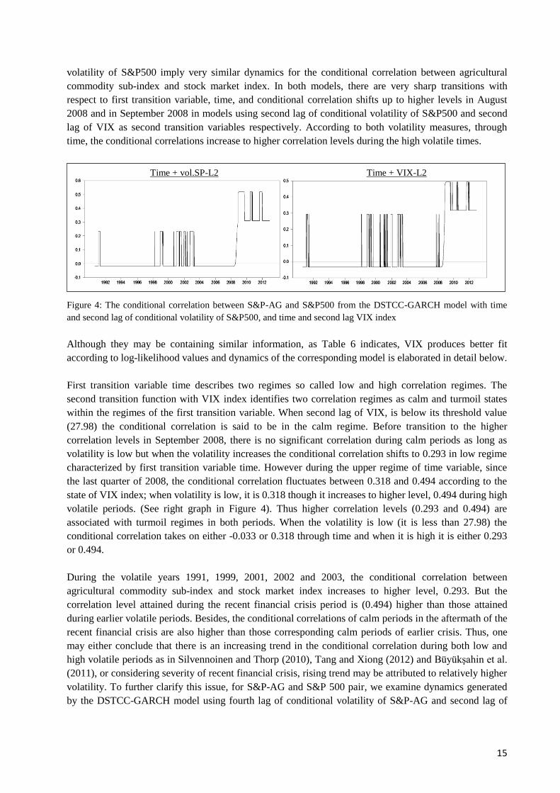
Figure 4: The conditional correlation between S&P-AG and S&P500 from the DSTCC-GARCH model with time

and second lag of conditional volatility of S&P500, and time and second lag VIX index

Although they may be containing similar information, as Table 6 indicates, VIX produces better fit

according to log-likelihood values and dynamics of the corresponding model is elaborated in detail below.

First transition variable time describes two regimes so called low and high correlation regimes. The

second transition function with VIX index identifies two correlation regimes as calm and turmoil states

within the regimes of the first transition variable. When second lag of VIX, is below its threshold value

(27.98) the conditional correlation is said to be in the calm regime. Before transition to the higher

correlation levels in September 2008, there is no significant correlation during calm periods as long as

volatility is low but when the volatility increases the conditional correlation shifts to 0.293 in low regime

characterized by first transition variable time. However during the upper regime of time variable, since

the last quarter of 2008, the conditional correlation fluctuates between 0.318 and 0.494 according to the

state of VIX index; when volatility is low, it is 0.318 though it increases to higher level, 0.494 during high

volatile periods. (See right graph in Figure 4). Thus higher correlation levels (0.293 and 0.494) are

associated with turmoil regimes in both periods. When the volatility is low (it is less than 27.98) the

conditional correlation takes on either -0.033 or 0.318 through time and when it is high it is either 0.293

or 0.494.

During the volatile years 1991, 1999, 2001, 2002 and 2003, the conditional correlation between

agricultural commodity sub-index and stock market index increases to higher level, 0.293. But the

correlation level attained during the recent financial crisis period is (0.494) higher than those attained

during earlier volatile periods. Besides, the conditional correlations of calm periods in the aftermath of the

recent financial crisis are also higher than those corresponding calm periods of earlier crisis. Thus, one

may either conclude that there is an increasing trend in the conditional correlation during both low and

high volatile periods as in Silvennoinen and Thorp (2010), Tang and Xiong (2012) and Büyükşahin et al.

(2011), or considering severity of recent financial crisis, rising trend may be attributed to relatively higher

volatility. To further clarify this issue, for S&P-AG and S&P 500 pair, we examine dynamics generated

by the DSTCC-GARCH model using fourth lag of conditional volatility of S&P-AG and second lag of

Time + vol.SP-L2 Time + VIX-L2

16

conditional volatility of S&P500 which delivers the best ML value. Estimated conditional correlations are

shown in Figure 5.

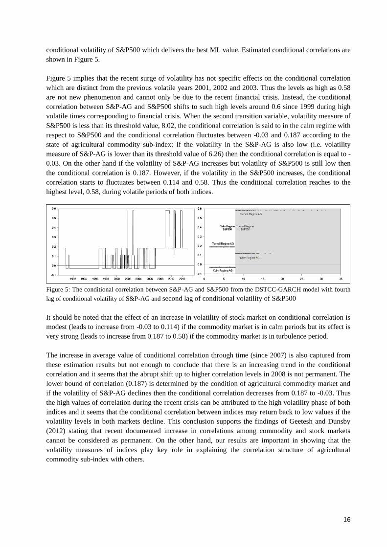
Figure 5 implies that the recent surge of volatility has not specific effects on the conditional correlation

which are distinct from the previous volatile years 2001, 2002 and 2003. Thus the levels as high as 0.58

are not new phenomenon and cannot only be due to the recent financial crisis. Instead, the conditional

correlation between S&P-AG and S&P500 shifts to such high levels around 0.6 since 1999 during high

volatile times corresponding to financial crisis. When the second transition variable, volatility measure of

S&P500 is less than its threshold value, 8.02, the conditional correlation is said to in the calm regime with

respect to S&P500 and the conditional correlation fluctuates between -0.03 and 0.187 according to the

state of agricultural commodity sub-index: If the volatility in the S&P-AG is also low (i.e. volatility

measure of S&P-AG is lower than its threshold value of 6.26) then the conditional correlation is equal to -

0.03. On the other hand if the volatility of S&P-AG increases but volatility of S&P500 is still low then

the conditional correlation is 0.187. However, if the volatility in the S&P500 increases, the conditional

correlation starts to fluctuates between 0.114 and 0.58. Thus the conditional correlation reaches to the

highest level, 0.58, during volatile periods of both indices.

Figure 5: The conditional correlation between S&P-AG and S&P500 from the DSTCC-GARCH model with fourth

lag of conditional volatility of S&P-AG and second lag of conditional volatility of S&P500

It should be noted that the effect of an increase in volatility of stock market on conditional correlation is

modest (leads to increase from -0.03 to 0.114) if the commodity market is in calm periods but its effect is

very strong (leads to increase from 0.187 to 0.58) if the commodity market is in turbulence period.

The increase in average value of conditional correlation through time (since 2007) is also captured from

these estimation results but not enough to conclude that there is an increasing trend in the conditional

correlation and it seems that the abrupt shift up to higher correlation levels in 2008 is not permanent. The

lower bound of correlation (0.187) is determined by the condition of agricultural commodity market and

if the volatility of S&P-AG declines then the conditional correlation decreases from 0.187 to -0.03. Thus

the high values of correlation during the recent crisis can be attributed to the high volatility phase of both

indices and it seems that the conditional correlation between indices may return back to low values if the

volatility levels in both markets decline. This conclusion supports the findings of Geetesh and Dunsby

(2012) stating that recent documented increase in correlations among commodity and stock markets

cannot be considered as permanent. On the other hand, our results are important in showing that the

volatility measures of indices play key role in explaining the correlation structure of agricultural

commodity sub-index with others.

17

S&P-PM – S&P500:

To have a comparison, S&P-PM and S&P500 pair is also examined. Table 5 clearly indicates that news

from both S&P-PM and S&P500 and volatility measures of S&P-PM and S&P500 carry significant

information after controlling for time trend. The estimation results of best model within each group, in

other words four DSTCC-GARCH models using time and second lag of error of S&P-PM, time and first

lag of error of S&P500, time and fourth lag squared error of S&P-PM, and time and first lag absolute

value error of S&P500 are reported in Table 6. The implied conditional correlations are depicted in Figure

6.

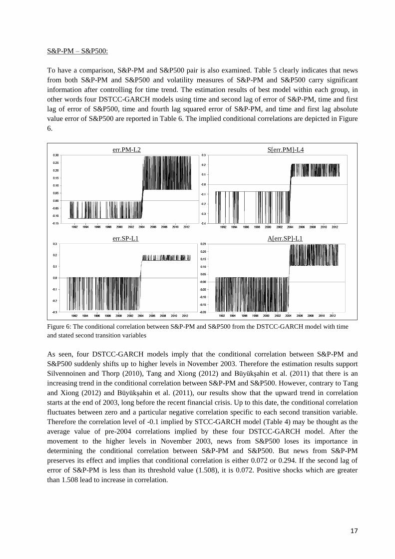
Figure 6: The conditional correlation between S&P-PM and S&P500 from the DSTCC-GARCH model with time

and stated second transition variables

As seen, four DSTCC-GARCH models imply that the conditional correlation between S&P-PM and

S&P500 suddenly shifts up to higher levels in November 2003. Therefore the estimation results support

Silvennoinen and Thorp (2010), Tang and Xiong (2012) and Büyükşahin et al. (2011) that there is an

increasing trend in the conditional correlation between S&P-PM and S&P500. However, contrary to Tang

and Xiong (2012) and Büyükşahin et al. (2011), our results show that the upward trend in correlation

starts at the end of 2003, long before the recent financial crisis. Up to this date, the conditional correlation

fluctuates between zero and a particular negative correlation specific to each second transition variable.

Therefore the correlation level of -0.1 implied by STCC-GARCH model (Table 4) may be thought as the

average value of pre-2004 correlations implied by these four DSTCC-GARCH model. After the

movement to the higher levels in November 2003, news from S&P500 loses its importance in

determining the conditional correlation between S&P-PM and S&P500. But news from S&P-PM

preserves its effect and implies that conditional correlation is either 0.072 or 0.294. If the second lag of

error of S&P-PM is less than its threshold value (1.508), it is 0.072. Positive shocks which are greater

than 1.508 lead to increase in correlation.

err.PM-L2 S[err.PM]-L4

err.SP-L1 A[err.SP]-L1

18

Both before and after the transition to the higher levels, the conditional correlation shifts down to lower

levels during the volatile periods of S&P-PM (i.e. when it is above its threshold value, 7.22). But there is

a structural change in the response of conditional correlation to the volatility of S&P500. Before the

transition, volatile times in S&P500 are associated with low correlations while they are with high

correlations after the transition.

S&P-AG – S&P-PM:

The constancy of conditional correlation between agricultural commodity and precious metal sub-indices

cannot be rejected in favor of STCC specification when time variable is employed in LM1 test. The best

STCC-GARCH model is produced by a volatility measure of S&P-PM, first lag of conditional volatility

of S&P-PM (Table 4), and estimation results imply that the conditional correlation between S&P-AG and

S&P-PM shifts from 0.132 to 0.365 when the volatility of precious metal index rises above its threshold,

5.385. The LM2 test results (Table 5) do not indicate time variable as significant transition variable in

none of the estimated STCC-GARCH models suggesting that increasing trend hypothesis is not valid for

S&P-AG – S&P-PM pair.

Figure 7: The conditional correlation between S&P-AG and S&P-PM from the DSTCC-GARCH model with stated

transition variables

DSTCC-GARCH models with all transition variable pairs reported in Table 5 are estimated and the

estimation results of two successful DSTCC-GARCH models are presented in Table 6. The implied

conditional correlations by these models are depicted in Figure 7. The left graph corresponds to the

DSTCC-GARCH model with two volatility measures of precious metal sub-index, namely third lag of

absolute value of error of S&P-PM and first lag of conditional volatility of S&P-PM. The estimated

correlation levels indicate that if the volatility of S&P-PM is low during the last three successive weeks,

the conditional correlation between commodity sub-indices (S&P-AG and S&P-PM) is very close to zero

(0.044). But during high volatile periods of S&P-PM, in addition to the inference from STCC

specification, DSTCC model reveals that the conditional correlation increases to high levels around 0.416

if the third lag of S&P-PM volatility is high, otherwise it increases to 0.193 (The correlation level implied

by STCC-GARCH model, 0.365, can be thought as the average of these respective levels). If this increase

in volatility of S&P-PM is followed by two calm weeks, the correlation reduces to 0.11 and if one more

calm week comes the correlation further reduce to 0.044 but if one turmoil week comes it increases to

0.193 again.

The estimated conditional correlation presented in the right graph of Figure 7 is generated by DSTCC-

GARCH model with second lag of conditional volatility of S&P-PM and third lag of squared error of

S&P-AG. During tranquil periods of both commodity market sub-indices (S&P-AG and S&P-PM), the

A[err.PM]-L3 + vol.PM-L1 vol.PM-L2 + S[err.AG]-L3

19

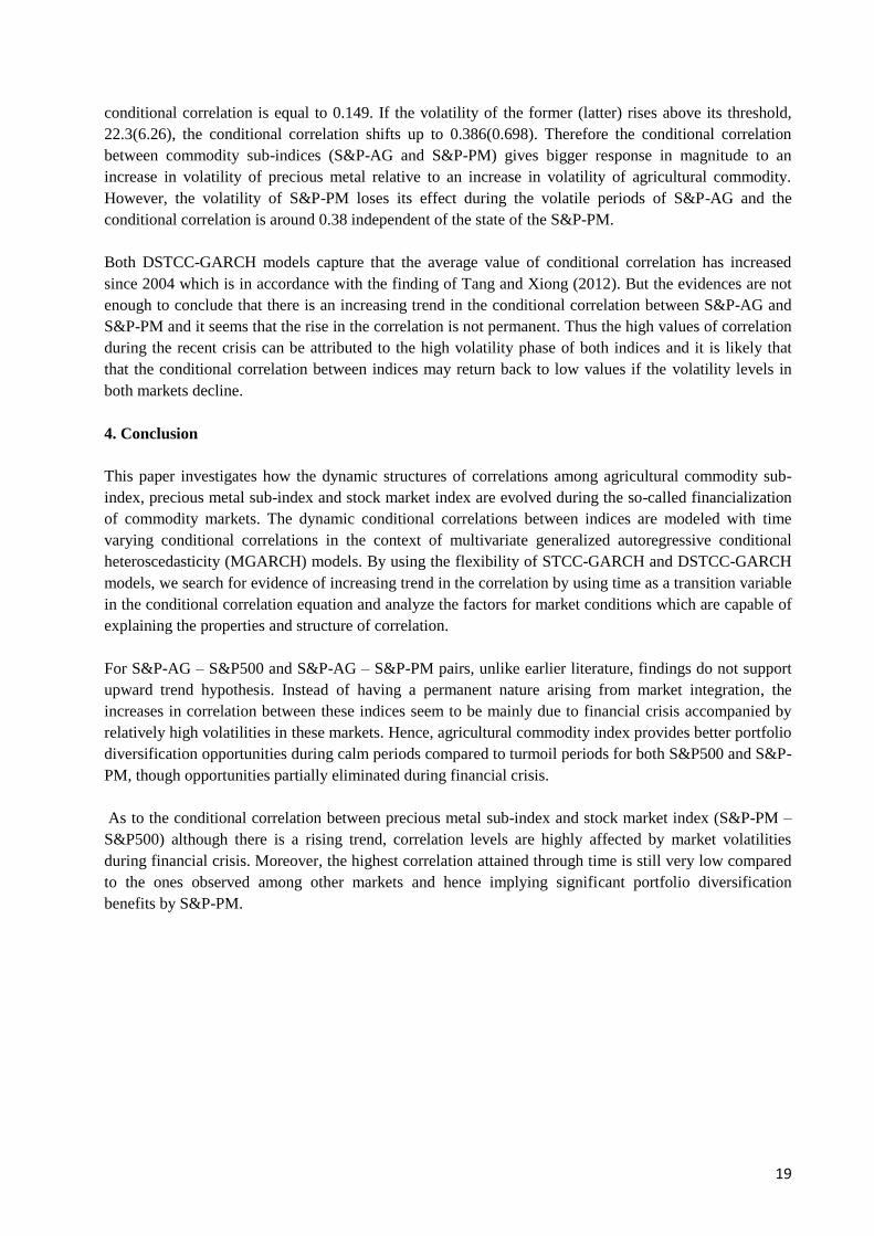
conditional correlation is equal to 0.149. If the volatility of the former (latter) rises above its threshold,

22.3(6.26), the conditional correlation shifts up to 0.386(0.698). Therefore the conditional correlation

between commodity sub-indices (S&P-AG and S&P-PM) gives bigger response in magnitude to an

increase in volatility of precious metal relative to an increase in volatility of agricultural commodity.

However, the volatility of S&P-PM loses its effect during the volatile periods of S&P-AG and the

conditional correlation is around 0.38 independent of the state of the S&P-PM.

Both DSTCC-GARCH models capture that the average value of conditional correlation has increased

since 2004 which is in accordance with the finding of Tang and Xiong (2012). But the evidences are not

enough to conclude that there is an increasing trend in the conditional correlation between S&P-AG and

S&P-PM and it seems that the rise in the correlation is not permanent. Thus the high values of correlation

during the recent crisis can be attributed to the high volatility phase of both indices and it is likely that

that the conditional correlation between indices may return back to low values if the volatility levels in

both markets decline.

4. Conclusion

This paper investigates how the dynamic structures of correlations among agricultural commodity sub-

index, precious metal sub-index and stock market index are evolved during the so-called financialization

of commodity markets. The dynamic conditional correlations between indices are modeled with time

varying conditional correlations in the context of multivariate generalized autoregressive conditional

heteroscedasticity (MGARCH) models. By using the flexibility of STCC-GARCH and DSTCC-GARCH

models, we search for evidence of increasing trend in the correlation by using time as a transition variable

in the conditional correlation equation and analyze the factors for market conditions which are capable of

explaining the properties and structure of correlation.

For S&P-AG – S&P500 and S&P-AG – S&P-PM pairs, unlike earlier literature, findings do not support

upward trend hypothesis. Instead of having a permanent nature arising from market integration, the

increases in correlation between these indices seem to be mainly due to financial crisis accompanied by

relatively high volatilities in these markets. Hence, agricultural commodity index provides better portfolio

diversification opportunities during calm periods compared to turmoil periods for both S&P500 and S&P-

PM, though opportunities partially eliminated during financial crisis.

As to the conditional correlation between precious metal sub-index and stock market index (S&P-PM –

S&P500) although there is a rising trend, correlation levels are highly affected by market volatilities

during financial crisis. Moreover, the highest correlation attained through time is still very low compared

to the ones observed among other markets and hence implying significant portfolio diversification

benefits by S&P-PM.

20

5. References

1. Ankrim, E. and Hensel, C. (1993). Commodities in asset allocation: A real asset alternative to

real estate. Financial Analysts Journal, 49(3), 2-9.

2. Barclays Capital, (2011). The commodity investors.

3. Becker, K.G. and Finnerty, J.E. (1994). Indexed Commodity Futures and the Risk of Institutional

Portfolios,” OFOR Working Paper, No. 94-02.

4. Bhardwaj, G. and Dunsby, A. (2012). The Business Cycle and the Correlation between Stocks

and Commodities. Working paper series available at http://ssrn.com/abstract=2005788

5. Bollerslev T. (1990). Modeling the coherence in short-run nominal exchange rates: a multivariate

generalized ARCH model. Review of Economics and Statistics, 72, 498-505.

6. Büyükşahin, B., Haigh, M. and Robe, M.. (2008), Commodities and equities: Ever a market of

one? Journal of Alternative Investments, 12, 76-95.

7. Büyükşahin, B. and Robe, M. (2009). Commodity Traders Positions and Energy Prices: Evidence

from the Recent Boom-Bust Cycle. Working paper, U.S. Commodity Futures Trading

Commission.

8. Büyükşahin, B. and Robe, M. A. (2011). Speculators, Commodities and Cross-Market Linkages.

Working paper.

9. CFTC Staff Report (2008). Commodity Swap Dealers & Index Traders with Commission

Recommendations.

10. Engle, R. F. (2002). Dynamic Conditional Correlation: A Simple Class of Multivariate

Generalized Autoregressive Conditional Heteroskedasticity Models. Journal of Business and

Economic Statistics, 20, 339–350.

11. Erb, C. B. and Harvey, C. R. (2006). The Tactical and Strategic Value of Commodity Futures.

Financial Analysts Journal, 62(2), 69-97.

12. Georgiev, G. (2001). Benefits of Commodity Investment. Journal of Alternative Investments,

4(1), 40-48.

13. Gorton, G. & Rouwenhorst, K. G. (2006). Facts and fantasies about commodity futures. Financial

Analysts Journal, 62(2), 47-68.

14. Greer, R.J. (2000). The Nature of Commodity Index Returns. Journal of Alternative Investments,

3, 45-53.

15. Hillier, D., Draper, P. and Faff, R. (2006) Do Precious Metals Shine? An Investment Perspective.

Financial Analysts Journal 62, 98-106.

16. Ocal, N. and Osborn, D.R. (2000). Business cycle non-linearities in UK consumption and

production. Journal of Applied Econometrics, 15(1), 27-43.

17. Silvennoinen, A. and T. Terasvirta (2005). Multivariate autoregressive conditional

heteroskedasticity with smooth transitions in conditional correlations. SSE/EFI Working Paper

Series in Economics and Finance No. 577

18. Silvennoinen, A. and Teräsvirta, T. (2009) Modeling multivariate autoregressive

heteroskedasticity with the double smooth transition conditional correlation GARCH model.

Journal of Financial Econometrics 7, 373-411

19. Silvennoinen, A. and Thorp, S. (2010). Financialization, Crisis and Commodity Correlation

Dynamics. Research Paper Series 267, Quantitative Finance Research Centre, University of

Technology, Sydney.

20. Tang, K. and Wei, X. (2012). Index Investing and the Financialization of Commodities. Financial

Analysts Journal, 68(6), 54-74.