Fe

dera

l Res

erve

Ban

k of

Chi

cago

Financialization in Commodity Markets

VV Chari and Lawrence J. Christiano

August, 2017

WP 2017-15

*Working papers are not edited, and all opinions and errors are the responsibility of the author(s). The views expressed do not necessarily reflect the views of the Federal Reserve Bank of Chicago or the Federal Reserve System.

Financialization in Commodity Markets

VV Chari and Lawrence J. Christiano⇤

August 15, 2017

Abstract

The financialization view is that increased trading in commodity futures markets is associated with

increases in the growth rate and volatility of commodity spot prices. This view gained credence be-

cause in the 2000s trading volume increased sharply and many commodity prices rose and became

more volatile. Using a large panel dataset we constructed, which includes commodities with and with-

out futures markets, we find no empirical link between increased futures market trading and changes

in price behavior. Our data sheds light on the economic role of futures markets. The conventional view

is that futures markets provide one-way insurance by allowing outsiders, traders with no direct interest

in a commodity, to insure insiders, traders with a direct interest. The data are not consistent with the

conventional view and we argue that they point to an alternative mutual insurance view, in which all

participants insure each other. We formalize this view in a model and show that it is consistent with

key features of the data.

Key Words: Spot Price Volatility, Futures Market Returns, Open interest, Net Financial Flows.

JEL Codes: E02, G12, G23.

⇤Chari: University of Minnesota and Federal Reserve Bank of Minneapolis; Christiano: Northwestern University and FederalReserve Banks of Chicago and Minneapolis. This research was supported by the Global Markets Institute at Goldman Sachs.We are grateful to Craig Burnside, James Hamilton and Mark Watson for insightful discussions of early versions of this paper,which led to substantial improvements. We are also grateful to Martin Eichenbaum, Anastasios Karantounias, Sergio Rebeloand Steve Strongin for their helpful comments. We are especially grateful to Husnu Cagri and Yuta Takahashi, for outstandingresearch assistance. The views expressed herein are those of the authors and not necessarily those of the Federal ReserveBanks of Chicago and Minneapolis, or the Federal Reserve System.

1

1. Introduction

Commodity markets are said to become more financialized when futures market trading volume rises rel-

ative to production. The financialization view is that increased trading activity is associated with increases

in commodity spot price growth and spot price volatility. This view gained credence because, starting in

the early 2000s, trading activity in commodity futures markets increased sharply relative to its level in the

1990s, while many spot prices rose and became more volatile. In this paper, we construct annual and

monthly datasets which contain panel data on 136 and 52 commodities, respectively. These data include

traded commodities, namely commodities with futures markets in the United States, as well as a variety

of non-traded commodities without such markets. The data allow us to investigate whether the prices of

traded and non-traded commodities behave differently and also allows us to investigate how the volume

of trade in a particular commodity affects the price behavior of that commodity. We find essentially no

support for the financialization view.

Our data also allow us to shed light on the economic role of futures markets. The conventional view

of such markets divides traders into insiders, firms and individuals with a direct commercial role in a

particular commodity, and outsiders, namely those individuals and firms without such an interest. Under

the conventional view, the role of futures markets is for outsiders to provide insurance to insiders. That

is, these markets provide one-way insurance. The Commodity Futures Trading Commission (CFTC)

classifies traders into categories that correspond to insiders and outsiders. We use the CFTC data to

measure the net long position of outsiders, which we refer to as net financial flows. Under the one-way

insurance view, the bulk of trading should consist of net financial flows. The data are simply inconsistent

with this view. Net financial flows account for only about 10 percent of open interest, the volume of

outstanding contracts. The bulk of open interest is due to insiders trading with each other and a smaller

fraction is due to outsiders trading with each other.

Another implication of the one-way insurance view is also inconsistent with the data. This implication

is that if outsiders are risk averse, increases in insurance demand by insiders in a particular commod-

ity should lead to an increase in the insurance premium charged by outsiders. This insurance premium

consists of the futures market returns earned on that particular commodity by outsiders. Thus, the con-

ventional view implies that when net financial flows are high for a particular commodity, expected futures

returns should also be high for that commodity. In the data, it turns out that there is no relationship

between net financial flows and returns.

These observations lead us to an alternative mutual insurance view in which futures markets are used

by insiders to insure each other, outsiders to insure each other, and both trading groups to insure each

other. That is, futures markets are a mutual insurance mechanism.

2

The challenge is to develop a model of the mutual insurance view, which is consistent with two key

features of the data: no relationship between net financial flows and returns and a positive relationship

between open interest and returns. We show that our model is consistent with both key features of the

data. In addition, it is consistent with the observation that net financial flows account for a small fraction

of overall volume.

Our model has two types of insiders, “farmers” who produce wheat, and “bakers” who use the wheat

to produce bread. For simplicity, we assume only one type of outsider. The demand for bread is affected

by shocks. One of these shocks is realized before production decisions are made, and is to be thought

of as a shock that affects the expected level of demand. The demand for bread is also affected by a

component which is correlated with outsiders’ income. This correlation fluctuates randomly. Outsiders

have incentives to use futures markets to insure themselves and the desire for this insurance fluctuates

due to fluctuations in the correlation.

All agents are risk averse and seek to use futures markets to purchase insurance if risks are high

relative to returns as well as to provide insurance if returns are high relative to risk. Farmers seek to

hedge risk, and this risk fluctuates with the expected level of demand. Bakers also seek to insure risk,

but their incentives to purchase insurance are weaker than those of farmers. The reason is that bakers

are partially hedged against price risk because when the price of wheat is high, so is the price of bread.

In the data, net financial flows are typically positive. To reproduce this feature in the equilibrium of our

model requires that outsiders be long on wheat futures. We choose parameters so that the equilibrium of

our model has this feature. Thus, in the equilibrium of our model, for all realizations of shocks, farmers go

short in the market and bakers and outsiders go long. Thus open interest consists of the sum of the long

position of outsiders and bakers, and net financial flows consists of the long positions of outsiders.

Consider now the response to various shocks. A positive shock to expected demand for bread in-

creases the risk faced by farmers who respond by increasing their insurance purchases and going further

short. Futures prices fall relative to the expected spot price, and so the expected return on futures rises.

This rise in expected returns induces outsiders to increase their supply of insurance and go further long.

It also induces bakers to go further long. The reason is that bakers’ concerns with risk are weaker than

those of farmers, but they still respond to returns. Since both bakers and outsiders increase their long

positions, open interest rises by more than net financial flows. Thus, in response to expected demand

shocks the covariance between open interest and returns is larger than that between net financial flows

and returns, and both are positive.

Consider next a correlation shock which tends to increase the long positions of outsiders. Such a

shock leads to a rise in futures prices and a reduction to the expected return in futures markets. Bakers

respond to this reduction in expected returns by reducing their long positions. Thus, the rise in open

3

interest is smaller than the rise in net financial flows. In response to correlation shocks, the covariance

between open interest and returns is larger than that between net financial flows and returns, and both

are negative.

Since the covariance between net financial flows and returns have opposite signs with respect to the

two shocks, there exists some value of the variances such that this covariance is zero. Using our previous

logic, at these parameter values the covariance between open interest and returns is positive. Given that

farmers and bakers can insure each other, our model is consistent with the observation that the bulk of

volume is accounted for by insiders trading with each other. Thus, our model is consistent with three key

features of the commodity futures markets: net financial flows are a small part of overall volume, there is

no relationship between net financial flows and returns, and there is a positive relationship between open

interest and returns.

Finally, our model is also consistent with the observation that there is no systematic relationship be-

tween financialization and spot price behavior. We assume that the variances of the exogenous shocks

differ across commodities and time. Outsiders must incur a fixed cost to participate in the market for a

given commodity, so that the extent of outsider participation is determined endogenously. With endoge-

nous participation, our model generates the lack of a systematic relationship between financialization and

spot price volatility.

Our empirical findings are based on an extensive data collection effort. For each commodity in our

data set we obtain spot price data and world production data from a variety of sources. In the case of

traded commodities, we use data on world production to scale the volume of futures trading. This scaling

is needed to allow trading activity across commodities and over time to be expressed in comparable

units. For non-traded commodities, the data on production is needed to develop indices of prices which

reflect each commodity’s economic importance. A separate Technical Appendix describes our data and

empirical methods in detail. In addition, we have assembled the data in a user-friendly form, which is

available upon request.

In order to evaluate the financialization view, we conduct two broad types of empirical analyses, a

decadal analysis, and a higher frequency analysis. The decadal analysis starts with the observation that

open interest is relatively constant in the 1990s at about one year’s worth of world production, and then

in the early 2000s it begins to grow rapidly and reaches about four year’s worth of world production by

2012. We ask whether the trend behavior and the volatility of prices is different in the periods before

2002 and after 2002. The idea is that some common change in financialization affected all commodities

at roughly the same time. We find that the distributions of the growth rates of prices across commodities

is indeed different across the two sub samples, but that this distribution changes in roughly the same way

for traded and non-traded goods. We look at a variety of measures of trend price growth and volatility and

4

find that none of decadal changes in these variables is systematically associated with associated decadal

changes in volume.

The higher frequency analysis allows for the extent of financialization to have changed at different

times for different commodities. In this analysis we find that the volatility of prices, measured as the stan-

dard deviation of prices over a moving window is not systematically associated with measures of volume.

We find that the distribution of volatilities shows a great deal of dispersion for non-traded commodities and

for commodities with low levels of volume but that for commodities with substantial amounts of volume,

the distribution is essentially unaffected by the level of volume.

Taken together, these findings suggest that the data provide no support for the financialization view.

We now elaborate on the empirical relationship between volume of trade for a particular commodity

and returns for that commodity. We investigate the ex post returns on different portfolio trading strategies.

We define the hot net financial flow strategy as a strategy in which a portfolio of commodity futures is

heavily weighted towards commodities where net financial flows have been high recently. We define

a random strategy as one that rebalances portfolios randomly. We find that the hot net financial flow

strategy generates returns that are similar to those on the random strategy. This result contradicts the

conventional view. We also consider an analogous hot open interest strategy. We find that this strategy

performs significantly better than the random strategy or a strategy based on a fixed portfolio of equities.1

The findings on the relationship between volume of trade and returns are related those in Hong and

Yogo (2012). The main focus of their analysis is on the relationship between aggregate measures of the

volume of trade and overall returns in futures markets for commodities. Our focus, in contrast, is on the

relationship between fluctuations in volume of trade and returns at the individual commodity level.

In terms of the relationship to the literature on the economic role of futures markets, the one-way

insurance view dates back to Keynes (1923), and Hicks (1939). See Hirshleifer (1990) for a more modern

rendering. Telser (1981) provides a succinct summary of the conventional view by saying “an organized

futures market furnishes legitimate businessmen with a means of hedging so they can obtain insurance

against price risk”. Challenges to this conventional view are also long standing (see Telser (1981), Cheng

and Xiong (2014) and Hong and Yogo (2012)).

Our analysis investigates the role of financialization by studying a broad cross section of commodities,

including a substantial number of non-traded commodities. In terms of non-traded goods, Irwin et al.

(2009), Kilian (2009), Kilian and Hicks (2013) look at the behavior of a few non-traded commodities. None

of the papers in the literature systematically study the behavior of the range of non-traded commodities

that we do.

In terms of our broad cross sectional analysis, much of the literature examines the role of financial-1We are grateful to Craig Burnside for suggesting this economically meaningful way to measure the relationship between

financialization and futures market returns.

5

ization on a specific commodity or groups of commodities. Even at the level of individual commodities,

the studies come to very different conclusions. Some studies such as Acharya et al. (2013), Brunetti

and Reiffen (2014), Etula (2013), Henderson et al. (2014), Masters (2008), Singleton (2014), Tang and

Xiong (2012) find evidence that supports the financialization view. Fattouh et al. (2013), Hamilton and

Wu (2015), Irwin and Sanders (2012), Irwin et al. (2009), Kilian and Murphy (2014), Stoll and Whaley

(2010) argue that the data does not support the financialization view. Brunetti and Buyuksahin (2009)

and Brunetti et al. (2016) argue that financialization reduces spot price volatility.

Section 2 describes our data and sources, sections 3 and 4 contain the decadal and high frequency

analysis. Section 5 contains our analysis of trading activity and returns in futures and other financial

markets. Finally, Section 6 contains description and analysis of a model which is consistent with our

empirical findings.

2. Data Description and Sources

2.1. Spot Price and Production Data

We construct a monthly dataset and an annual dataset for a variety of commodities to study the associa-

tion between futures trading and market outcomes. For 29 commodities, referred to here as traded com-

modities, monthly and annual futures markets volume data can be constructed from the CFTC dataset.

For the rest of the commodities in our dataset the CFTC does not track futures trading, typically because

such futures markets do not exist, at least in the United States. We refer to these commodities as non-

traded commodities. We also subdivide commodities into various subcategories. In particular, we sort

the data into softs (i.e., agricultural commodities like corn and lumber), minerals and fuels. We also sort

traded commodities according to whether they are included in widely-used indices.2

We gathered spot price data for commodities for which annual world production data are available.

Monthly and annual spot market price data are available for our traded commodities from a variety of

sources (see Table 1 for the annual data, and Table 2 for the monthly data). For 23 non-traded com-

modities, we were able to obtain monthly spot price data from a variety of sources (see Table 3) and

for 107 commodities we were able to obtain annual spot price data from British Petroleum, the US Geo-

logical Survey and the United Nations Food and Agricultural Organization (see the Technical Appendix).

The tables also report the subcategories to which each commodity belongs. Note that the sets of non-

traded commodities covered in the monthly and annual data are different, so that the results for these two2Following Tang and Xiong (2012) we identify commodities traded on futures exchanges as ’indexed’ if in 2008 they receive

non-zero weight in both the basket of commodities in the Standard and Poor’s Goldman Sachs commodity index (S&P GSCI)and the commodities in the Dow Jones-UBS commodity index (DJ-HBSCI).

6

datasets need not be the same.

2.2. Futures Market Volume Data

Monthly and annual data on the volume of activity in futures markets can be obtained from a weekly

dataset provided by the CFTC for our 29 commodities. For our annual dataset, for each commodity we

sum the CFTC data over all the contracts within each year. We scale our measures of volume in each year

by world production of the underlying commodity in the same year. This scaling ensures that our measure

of volume is comparable across commodities and captures the notion that the market for commodities is

more financialized if the volume of futures trade is larger relative to production for that commodity. Table

1 reports our sources for world production of traded goods. For our monthly data set we convert the

CFTC data into monthly terms by summing over all the contracts within each month. We interpolate the

annual world production data to obtain monthly world production. We then scale monthly open interest by

monthly world production for each commodity.

Motivated by our interest in measuring the extent to which insiders and outsiders insure each other, we

construct a second measure of futures trade volume, which we call net financial flows. We construct this

measure using the positions in futures markets of insiders and outsiders, reported by the CFTC. Specif-

ically, the CFTC categorizes futures market trades as commercial, non-commercial and non-reported.3

A trade is classified as commercial if the associated trader is operating on behalf of entities whose main

business is in the production, sale or use of the relevant commodity, and if the trader’s position at the

end of the day is sufficiently large. A trade is classified as non-commercial if the associated trader is not

operating on behalf of such a business and if the trader’s position at the end of the day is sufficiently large.

Both these types of trades are referred to as reported. A trade is non-reported if the trader’s position at

the end of the day is not sufficiently large. In this case, the CFTC does not report whether the trade is

commercial or non-commercial.

We categorize all commercial trades as trades by insiders and all non-commercial trades as trades

by outsiders.4 We allocate non-reported trades at each date to the insider and outsider categories in

proportion to the share of commercial and non-commercial trades respectively in total reported trades at

that date. For each commodity, i, and date, t, let SLit denote the gross long positions of outsiders, summed

across all outstanding futures contracts in commodity i at datet, scaled by date t world production. Let Ssit

denote the analogous short positions. Let HLit and Hs

it denote the analogous positions for insiders. With

3For details, see http://www.cftc.gov/MarketReports/CommitmentsofTraders/ExplanatoryNotes/index.htm.4To obtain the gross long and short positions of non-commercial trades from the CFTC data requires some care. The CFTC

reports the sum, across traders, of their net long and short positions, as well as the sum of a variable they refer to as thespread. The spread is the sum, across all traders, of the position (long or short) that is smaller. The sum of the net longpositions and the spread gives the gross long positions and similarly so, for the short positions.

7

this notation, open interest, oiit, and net financial flows, nffit, for commodity i at date t are given by:

oiit = SLit +HL

it = Ssit +Hs

it

nffit = SLit � Ss

it = ��HL

it �Hsit

�. (1)

We also use data on returns on futures contracts. To construct these returns we use the daily prices

for futures contracts of various maturities for the commodities used in Tang and Xiong (2012), kindly

provided to us by the authors.

3. Spot Price Behavior and Financialization: Decadal Analysis

In this section we document that open interest is substantially higher in the 2000s than in the 1990s.

Under the financialization view, this increase in trading activity should be associated with a change in

the behavior of spot prices. To the extent that common factors across all commodities, such as taxes,

regulation, digital technology, institutional innovation and attitudes towards risk, drove the increase in

open interest, we would expect the behavior of the prices of all commodities to be different in the 2000s

than in the 1990s. We investigate this implication of the financialization view in this section. We then go

on to allow the extent of financialization to differ across commodities in the 1990s and 2000s, but maintain

the perspective that these changes all occurred at roughly the same time.

We find no consistent change in behavior among commodities. This finding undercuts the financial-

ization view.

3.1. Patterns in Trade Volume

To characterize the general movements in volume of trade, we construct indices. We construct a trade

volume index for commodities by weighting a measure of trade volume for each commodity by the average

value of its share in world production. Specifically, for open interest, let oiit denote the volume of open

interest in commodity i in period t, scaled by world production, qit. The open interest index, oit, for period

t is given by

oit =X

i

wioiit,

where the weight, wi, is given by

wi =1

T

X

t

PitqitPj Pjtqjt

.

Here, Pit denotes the spot price of commodityi in periodt. We construct the index of net financial flows,

nfft, in a similar fashion. The price indices are constructed in a similar fashion, except that we scale

8

Pit by the periodt personal consumption expenditure deflator and we normalize the index, Pt, so that its

value is unity at t = 0.

Figure 2 displays annual and monthly data for our index of open interest and of net financial flows. We

emphasize two features of the data that are apparent from this figure. First, open interest is substantially

greater than net financial flows at every date. Second, our index of open interest behaves very differently

in the 1990s than it does in the 2000s.

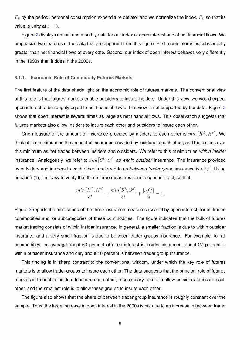
3.1.1. Economic Role of Commodity Futures Markets

The first feature of the data sheds light on the economic role of futures markets. The conventional view

of this role is that futures markets enable outsiders to insure insiders. Under this view, we would expect

open interest to be roughly equal to net financial flows. This view is not supported by the data. Figure 2

shows that open interest is several times as large as net financial flows. This observation suggests that

futures markets also allow insiders to insure each other and outsiders to insure each other.

One measure of the amount of insurance provided by insiders to each other is min⇥HL, Hs

⇤. We

think of this minimum as the amount of insurance provided by insiders to each other, and the excess over

this minimum as net trades between insiders and outsiders. We refer to this minimum as within insider

insurance. Analogously, we refer to min⇥SL, Ss

⇤as within outsider insurance. The insurance provided

by outsiders and insiders to each other is referred to as between trader group insurance is|nff |. Using

equation (1), it is easy to verify that these three measures sum to open interest, so that

min⇥HL, Hs

⇤

oi+

min⇥SL, Ss

⇤

oi+

|nff |oi

= 1.

Figure 3 reports the time series of the three insurance measures (scaled by open interest) for all traded

commodities and for subcategories of these commodities. The figure indicates that the bulk of futures

market trading consists of within insider insurance. In general, a smaller fraction is due to within outsider

insurance and a very small fraction is due to between trader groups insurance. For example, for all

commodities, on average about 63 percent of open interest is insider insurance, about 27 percent is

within outsider insurance and only about 10 percent is between trader group insurance.

This finding is in sharp contrast to the conventional wisdom, under which the key role of futures

markets is to allow trader groups to insure each other. The data suggests that the principal role of futures

markets is to enable insiders to insure each other, a secondary role is to allow outsiders to insure each

other, and the smallest role is to allow these groups to insure each other.

The figure also shows that the share of between trader group insurance is roughly constant over the

sample. Thus, the large increase in open interest in the 2000s is not due to an increase in between trader

9

group insurance. Instead, it is associated with a sharp increase in within outsider insurance.

3.1.2. Patterns in Trade Volume: Decadal Analysis

The second feature of Figure 2 that we emphasize is that our index of open interest displays no trend and

averages roughly a little over one year’s production until the early 2000s. It then rises sharply up to a little

over four times world production by the end of our sample, 2012. Net financial flows are nearly zero in the

first half of the sample and are somewhat higher in the second half of the sample. Figure 2 shows that

there is a volatile high-frequency component in the monthly data. In the Technical Appendix, we show

that this volatility is not driven by seasonal movements.

Open interest in the second half of the sample is substantially greater than in the first half. Under the

financialization view the behavior of commodity prices in the second half of the sample should be very

different from its behavior in the first half of the sample. We investigate this implication in the remainder

of this section.

3.1.3. Patterns in the Behavior of Price Indices

We begin by displaying the log of the price index for the commodities in our dataset in Figure 1. The

dashed line in this figure displays the time series behavior of the index based on the 136 commodities in

the annual dataset. The solid line displays the index for the 52 commodities in our monthly dataset.

Figure 1 gives the impression that the behavior of commodity prices did indeed change at roughly the

same time that activity in the futures markets increased. This visual inspection apparently supports the

financialization view. The eye could be misled, however, by a chance sequence of positive growth rates

early in the second sub sample. To guard against this possibility, we conduct tests of the null hypothesis

that the mean growth rates in the two sub samples are the same. The p�values reported in the figure

show that these tests fail to reject the null hypothesis. Thus, the visual evidence could just be an artifact

of chance. In this sense, the data do not offer compelling evidence for the financialization view.

Under the financialization view, we would expect the change in price behavior to be greater for traded

commodities than for non-traded commodities. We investigate this implication by decomposing our ag-

gregate commodity price index into traded and non-traded goods. Panel A of Figure 4, which uses our

annual data set, gives the impression that the behavior of the prices of traded goods is different in the

two sub samples and the behavior of non-traded goods is not very different in the two sub samples. This

figure shows that the price of traded goods rises at best moderately in the first half of the sample and

rises more quickly in the second half of the sample. Furthermore the price of traded goods seems to be

more volatile in the second half of the sample than in the first.5 In contrast, the price of non-traded goods5The index for all goods behaves very similarly to the index for traded goods because traded goods account for a large

10

rises at about the same rate in both halves of the sample and does not display an increase in volatility.

In panel A of Figure 4 we also report p�values for the same test as in Figure 1. The p�values indicate

that the data in Figure 4 do not offer compelling evidence for the financialization view.

We now turn to our monthly data. Panel B of Figure 4 shows that traded goods prices display a

similar pattern as in Panel A. This pattern is not surprising because the underlying commodities are the

same in both cases. The underlying commodities are different for non-traded goods. As can be seen

from Panel B, the price behavior of the non-traded goods in our monthly data set is different from the

behavior of our annual dataset displayed in Panel A. In the first half of the sample, the price of non-traded

goods appears to fall and then rises in the second half of the sample. Panel B of Figure 4 gives the

impression that non-traded goods prices behave very differently in the two sub samples and that traded

goods behave somewhat differently. The p�values reported in the figure show that non-traded goods

prices are indeed statistically significantly different in the two sub samples, while traded good prices are

not statistically significantly different. The financialization view leads to exactly the opposite implication

for the data. Thus, the results in this figure undercut the financialization view.

In sum, visual inspection of the annual data suggests that the financialization view should be taken

seriously. The monthly data undercuts the financialization view and statistical tests do not provide com-

pelling evidence for the view.

This mixed message leads us to bring more data to address our question. We use data on the

behavior of the prices of individual commodities and the extent of financialization in the market for that

commodity.

3.1.4. Patterns in the Behavior of Individual Commodity Prices

Here, we bring to bear our data from a large number of commodities traded in a variety of markets to

investigate the financialization view. For each commodity, we compute the mean and standard deviation

of the one-period growth rate of its log price in the 1990s and the 2000s. We ask whether these means

and standard deviations are significantly different in the two sub samples. In effect, this comparison

asks whether changes in price behavior comove with changes in aggregate financialization. We go on

to investigate the comovement between changes in price behavior for each commodity in the two sub

samples and changes in volume of trade for that commodity. We do not find compelling evidence for the

financialization view, either at the aggregate level, or at the individual commodity level.

Mean Growth Rates of Commodity Spot Prices

Consider first the average of mean growth rates, for all commodities as well as various subgroups.

Table 4 reports the cross-sectional average, across commodities in the relevant group, of the mean growth

fraction of world production of all commodities.

11

rates and associated standard deviations in the two sub samples. The table also reports p�values for the

test of the null hypothesis that the statistics are the same in both periods.6 This table shows that these

averages are higher in the 2000s than in the 1990s, but that the difference is not statistically significant in

the annual data. This finding is similar to that for the indexes reported in Panel A of Figure 4. The findings

for the monthly data for the subcategories of traded and non-traded goods are also similar to those in

Panel B of Figure 4. Note that, unlike the findings in Panel B of Figure 4, here the average of the mean

growth rates for all commodities is significantly higher in the second half than in the first half. The reason

the results are different is that the index assigns a very substantial weight to traded commodities, while in

Table 4 each commodity receives equal weight.

Consider next the growth rate of prices for each commodity. This growth rate displays substantial

heterogeneity across commodities. In Figure 5, we report the empirical density functions of commodity

growth rates in the two sub samples, for all commodities as well as for traded and non-traded commodi-

ties. The panels for all commodities show that the distribution of growth rates of commodity is differ-

ent in the two sub samples. These distributions are statistically significantly different according to the

Kolmogorov-Smirnoff test. The observation that these distributions are statistically significantly different

is not inconsistent with our observation that the means from these distributions are statistically insignif-

icantly different from each other. The figure shows that the mean from each sample is well inside the

distribution of the other sample.

At first glance, the observation that, for all commodities, the distributions are significantly different

from each seems to provide support for the financialization view. The panels for traded and non-traded

commodities undercut that support. We see in that the shift in distribution occurs for both traded and

non-traded goods, and so seems to have nothing to do with financialization.

Overall, the findings here reinforce the findings from the index analysis that the data do not provide

compelling evidence for the financialization view.

Averages of Volatility of Spot Prices

Table 4 shows that differences in the volatility of spot price growth across the two sub samples are

in general not significantly different.7 The differences are significant only for non-indexed commodities

and marginally significant for traded commodities. The table also shows that the volatility of the growth

rate of spot prices of non-traded goods is higher than that of traded goods. Thus, there is no compelling

evidence here in support of the financialization view.

Commodity-Level Comovement Between Spot Prices and Volume6These tests were constructed using both a bootstrap method and a sampling theory described in the Technical Appendix.7Volatility statistics are expressed in annual, percent terms. In the case of monthly data, we do this by multiplying the

monthly standard deviation by100p12. This conversion is the correct one if monthly price data are a logarithmic random walk.

12

We continue to maintain the decadal perspective, except that we allow the extent of financialization to

differ across commodities. We ask whether the data show a significant relationship between changes in

spot price behavior and changes in the volume of trade, namely, open interest and net financial flows, for

each commodity.

Specifically, for each commodity in our data set, we compute three statistics for each of our two sub

samples. The first is the change, over the two sub samples, in the standard deviation of the growth rate

of prices. The second and third statistics are based on a linear regression of the log, real commodity

price on a time trend and a constant, allowing the coefficients to be different in the two sub samples. The

second statistic is the change in coefficient on the time trend and the third statistic is the change in the

standard deviation of the regression error term. All statistics are report in annual percent terms.

We ask whether our statistics are large when the change in the average volume of trade across the

two sub samples is large. We answer this question by regressing our statistics on the corresponding

change in volume of trade. Our measures of volume of trade are open interest and net financial flows,

scaled by world production. Table 5 reports the probability, under the null hypothesis that the coefficient

on volume of trade higher than its estimated value. The rows of Table 5 correspond to different categories

of commodities. Table 5 displays the coefficients of these regressions as well as tests of statistical signifi-

cance. This table shows that, with one exception, the coefficients are not significantly different from zero.

The exception is that, in the case of softs, changes in the coefficient on the time trend are significantly

associated with changes in both measures of volume.

We illustrate this exercise in Figure 6. Each panel of the figure is a scatter plot for all commodities

and subcategories of commodities. Our second statistic, the change in the coefficient on the time trend,

is on the vertical axis and the change in open interest is on the horizontal axis. For convenience, the

figure also reports the corresponding entries from Table 5, namely the estimate regression slope term

and associated p�value. Except for softs, each panel shows a cloud without a clear pattern.

The sense in which there is no systematic relationship between changes in open interest and changes

in price behavior can be seen by considering the behavior of gold and silver. Using our annual dataset, we

see that open interest in gold increased by about 12 times world production, while open interest in silver

declined by about 5 times world production. In both cases, the coefficient on the time trend increased by

about 20 percentage points, at an annual rate.

Visual inspection of Figure 6 and the results in Table 5 show that, with the exception of softs, there is

no compelling evidence for the financialization view.

13

4. Patterns in Price Behavior: Higher Frequency Analysis

The decadal approach in the previous section takes the stand that changes in financialization took place

at roughly the same date for all commodities. Here, we allow for the possibility that variations in finan-

cialization occurred at different dates for different commodities. We ask whether, in our monthly dataset,

higher levels of financialization are systematically associated with higher volatility of spot prices.

To answer this question we measure volatility by the plus and minus 2 year centered moving average

of the standard deviation of the logarithmic growth rate of commodity prices. Figure 10 is a scatter

plot of our measure of volatility against our two measures of volume for all commodities and for various

subcategories of commodities. Each point in the figure is a volatility, volume combination for a specific

commodity at a particular date. The upper and lower panels of the figure are based on our annual and

monthly datasets, respectively. As before, the volatility measures are converted to annual, percent terms.

The figure shows that when trading volume is near zero, volatility measures are on average higher and

more dispersed than when trading volume is substantial. This finding suggests that higher financialization

is associated with lower volatility of spot prices. In this sense, the data contradict the financialization view.

In each case, the line in the figures is the least squares line through the data, with the slope indicated

in the associated figure header. These slopes are not significantly different from zero at the five percent

level (see Table 6)8. Furthermore, except for softs, all the coefficients are negative but quantitatively

small. For example, for all commodities and the monthly data, the reported slope implies that an increase

in open interest of one year’s production is associated with a 0.13 percentage points reduction in the

standard deviation of price growth.

We also regressed the volatility of each commodity on our measures of volume, and display the

frequency distribution of the slope coefficients in Figure 11. That figure indicates that the distribution,

though dispersed, is centered on negative slopes, for both our measures of volume. Thus, there is

no evidence that with greater trading volume, volatility goes up. On the contrary, there is modest, not

statistically significant, evidence that that volatility actually goes down with increased volume.9

Another way of seeing that financialization has essentially no impact on commodity price volatility is

with a quartile analysis. In particular, we examine how the distribution of our measure of price volatility

depends on our measures of volume. We measure spot price volatility by the standard deviation of

spot price growth. For each measure of volume, we restrict attention to the price volatility observations

that lie in the second and third quartiles of volume. Panels a and b in Figure 14 report the histograms,

means and modes of volatility for the second and third quartiles, sorting on open interest and net financial8In computing the sampling uncertainty for the coefficients, we dropped four commodities, butter, propane, aluminum and

coal because there is so little trade.9A Kolmogorov-Smirnov goodness-of-fit hypothesis test on the null hypothesis that the two histograms in Figure11 are

sampled from the same underlying population fails to reject at the 5 percent level.

14

flows, respectively. From Panel a is clear that the distributions of volatility are essentially identical for

observations that lie in the second and third quartile of open interest. Panel b shows that the distribution

of volatility in the third quartile lies slightly to the right of the distribution in the second quartile. This

difference is quantitatively small. For example, the mean of volatility in the third quartile is 27.4 percent

and it is 24.4 percent in the second quartile. These findings suggest that there is essentially no empirical

link between financialization and commodity price volatility.

5. Trading Volume and Properties of Futures Returns

Here, we examine the relationship between financialization and the behavior of returns in futures markets.

First, we consider the relationship between measures of volume and returns. We find that when open

interest growth over the preceding 12 months is high, futures returns over the next month also tend to be

higher. In this sense, high growth in open interest tends to predict high returns in futures markets. We find

no such relationship between net financial flows and returns in futures markets. Second, we consider the

relationship between returns in futures markets and returns in equity and Treasury markets. In particular,

we examine the correlation between returns in various markets and measures of financialization. While

the daily data suggests that the correlation in returns among markets rises with financialization, in the

monthly data the change in the correlation is not significant.

5.1. Open Interest, Net Financial Flows and Futures Returns

In order to analyze the relationship between futures returns and past trading volume, we consider portfolio

strategies in which assets are allocated according past volume. Specifically, in each month in the period

1960-2008, we select the one-third of our commodities which had the highest volume of futures market

trade.10 When our measure of volume is open interest, we work with the growth rate of aggregate open

interest in the preceding 12 months and when our measure is net financial flows, we use the imbalance

measure used in Hong and Yogo (2012). This imbalance measure is closely related to our measure of

net financial flows.

We then compute the returns associated with a strategy of buying long contracts in each of the com-

modities inside the group with the largest past volume of trade. For open interest, we refer to this strategy

as the hot open interest strategy. For net financial flows we refer to the strategy as the hot net financial

flow strategy. We also consider a random strategy in which the portfolio of commodities in each month is

selected randomly. We compute 200,000 sequences of returns associated with this strategy by repeated

random draws over the whole data sample.10We use the data employed in Hong and Yogo (2012), which they kindly shared with us.

15

Figure 12 shows the cumulative returns for the hot strategies as well as some statistics for the random

strategy. The figure reports the median cumulative return, as well as the 10th to 90th percentiles of

the cumulative returns for the random strategy. The figure shows that the hot open interest strategy

outperforms 90% of the random strategies over the entire sample, while the hot net financial flow strategy

performs approximately as well as the median random strategy. Furthermore, the figure shows that the

hot open interest strategy outperforms 90 percent of the random strategies from 2000 onwards.

In Figure 13 we plot the distribution of Sharpe ratios associated with the random strategy, as well as

the Sharpe ratios for the two hot strategies. These Sharpe ratios are computed by taking the ratio of

the average monthly excess return over the corresponding return from holding 3-month Treasury bills,

to the standard deviation of this excess return. The figure shows that the Sharpe ratio for the hot open

interest strategy, 0.13, is well above the mean Sharpe ratio of the random strategy, 0.08, while the Sharpe

ratio for the hot net financial flow strategy, 0.09, is not very different from the random strategy. The

p�value for testing the null hypothesis that the hot open interest Sharpe ratio is drawn from the random

strategy distribution is 0.007, while the associated p�value for the hot net financial flow strategy is 0.44.

Interestingly, the Sharpe ratio on the hot open interest strategy also dominates the Sharpe ratio for the

value-weighted monthly excess return on equity. Using monthly return data over the period, 1960-2008,

the Sharpe ratio for equity is 0.072.11

These results suggest that when the value of outstanding futures contracts at the beginning of a month

are high, futures returns during that month are also high. The figures also show that the data show no

such relationship between net financial flows and futures returns.

5.2. Comovement of Returns Across Markets

Next, we examine the comovement of returns across markets. This examination is motivated by the

findings of Tang and Xiong (2012), which suggest that financialization affected return comovement.12

Comovement and Volume of Trade

For each year we use the data on asset returns within that year to compute three statistics: two pairwise

correlations and the standard deviation on futures returns. The two pairwise correlations are between

futures and equity returns and between futures and T-bill returns. We compute these three statistics for

each year in our sample using daily as well as monthly returns.11Our equity return data are equally weighted daily equity returns taken from the Center for Research on Securities Prices

(CRSP) database. These returns were aggregated into monthly returns in Ferreira (2013), and we are grateful to the authorwho kindly shared his data with us. We obtained daily and monthly returns on 3 month US government treasury bills from theonline data base, FRED, maintained by the Federal Reserve Bank of St. Louis.

12We are grateful to Tang and Xiong for kindly sharing their data with us.

16

We are interested in understanding how the pairwise correlation between returns on futures contracts

and on equity and T-bills moves with changes in financialization. For each of 27 commodities, we study

the relationship between the three statistics just described and our two measures of financialization. To

this end, we run the following regression:

yt = ↵ + �xt + ut, t = 1992, ..., 2009, (2)

where yt is one the three statistics described and xt is our measure of volume. Our results are displayed

in Table 7. That table reports the average value of the �’s across the 27 commodities. The table shows

that, apart from one case, the average value of � is not statistically significantly different from zero.13

The monthly data show no evidence of a link between financialization and the volatility of returns or the

comovement of returns between futures markets and equity or Treasury markets.

5.2.1. Comovement and Indexation

Next, we look for the effects of financialization by investigating whether the comovement properties of a

commodity depend on whether or not it is included in the two popular commodity indexes. Using daily

return data, Tang and Xiong (2012) show that the pairwise correlation among commodities included in the

indices rose sharply after 2004, relative to the increase for non-indexed commodities. Their results are

reproduced in the 1,1 panel of Figure 15.14 We then redid the calculations using monthly observations

on monthly returns and those results are displayed in the 2,2 panel of the figure. Note that now it makes

little difference whether the correlations are between commodities that are included in an index or not. To

understand the reason for the different properties of daily and monthly data, we went back to the daily

data and redid the Tang and Xiong calculations when returns are 10 day returns and 20 day returns. The

results are displayed in the 1,2 and 2,1 panels of Figure 15, respectively. Note that when the 10 day

returns are considered, the difference between indexed and non-indexed commodities is substantially

smaller than it is in the case of one-day returns. By the time we consider 20 day returns, the differences

are nearly gone.

We obtain similar results when we consider the average of correlations between commodity futures

and the return on equity. Panel a in Figure 16 displays the correlations based on daily returns. Note that

it makes a noticeable difference for the correlation, whether or not a commodity is included in the indices.

Panel b shows that the difference is gone when the correlations are computed using monthly returns.

In the Technical Appendix we explore the idea that the difference between the monthly and daily data13Consistent with the findings of Tang and Xiong (2012), this coefficient is significantly positive in the daily data.14To construct these correlations, for each pair of commodities and each date, we computed a correlation between returns

on the two commodities, using a centered 13 month window of data. For each month, we then computed the average of allthat month’s pairwise correlations.

17

can be accounted for by technical details not related to economic fundamentals, about the functioning of

futures markets. In any event, in our view the monthly data are likely to be more relevant for determining

production, consumption and spot prices of commodities.

In sum, the data suggest that high levels of open interest are associated with high expected futures

returns and net financial flows show no relationship with returns.

6. Model of Futures Markets

The empirical findings described so far can be summarized broadly by the following stylized facts.

1. There is no systematic relationship between the volume of trade in the futures markets for a

particular commodity and the behavior of spot prices, particularly the volatility of spot prices for that

commodity.

2. There is a positive association between open interest and futures market returns, in the sense that

high levels of open interest are associated with a subsequent above average return in futures markets.

3. The correlation between net financial flows and futures markets returns is roughly zero.

Here we develop a simple model of futures markets which is consistent with these stylized facts. The

model suggests that futures markets play an important social role that has not been emphasized in the

conventional view of the economic role of futures markets. The conventional view emphasizes the idea

that futures markets allow "insiders", namely firms and individuals who have a direct commercial role in

a particular commodity to purchase insurance from "outsiders’, namely those individuals and firms who

have no direct commercial interest in the particular commodity. In this conventional view, insiders are

referred to as hedgers and outsiders as speculators. The conventional view suggests that net financial

flows should be positively correlated with returns in futures markets. The reason is that the outsiders, if

they are risk averse, should be compensated for the insurance they provide to insiders. The conventional

view also suggests that when the hedging needs of insiders are large, open interest should be high and

so should net financial flows. As we have seen, the data on net financial flows does not support this

implication of the conventional view.

Here we argue that the data suggests an alternative view. In this alternative view, futures markets are

used by insiders to insure each other, outsiders to insure each other, and both trading groups to insure

each other as well. We formalize this alternative view by developing a model with two key features. First,

in our model, futures markets allow outsiders to use futures markets to insure against risks confronting

their incomes and portfolios. Second, in our model some insiders wish to purchase insurance and other

insiders wish to sell insurance. Thus, futures markets allow outsiders to insure themselves and insiders to

insure each other. In our model, futures markets provide a valuable mutual insurance role that is absent

18

in the conventional view.

We begin by describing the model and then highlight the key features of the model. We consider

a static model of trade in an intermediate good labeled "wheat" for convenience. Wheat is produced

by "farmers" and transformed by "bakers" into a final consumption good labeled "bread". Farmers and

bakers are "insiders’ in the sense that they have a direct commercial interest in the wheat market. Our

model also has a third type of agents, "outsiders’ who have no direct commercial interest in the wheat

market. The demand for bread is affected by shocks and the income of outsiders is also stochastic. We

assume that the correlation between outsiders’ income and bread demand fluctuates. This correlation

creates a desire on the part of outsiders to use futures markets as an insurance device. Fluctuations in

this correlation imply that in some situations, outsiders could be insuring insiders and in other situations,

insiders could be insuring outsiders.

Our modeling of trade in an intermediate good is, in part, motivated by the observation that, in practice,

almost all futures markets trade in intermediate goods, rather than final goods or raw materials. This way

of modeling trade allows us to develop a sharp distinction between open interest and net financial flows.

The idea is that, in the model, as in the data, a significant amount of futures trade is among insiders

rather than between insiders and outsiders. In our model, farmers and bakers use futures markets to

insure each other against fluctuations in the price of bread, and much of the volume of trade is between

these parties.

Our modeling of the shocks is intended to capture the idea that outsiders might wish to trade in futures

markets to hedge against risks to their income. Such trade is valuable if spot prices of bread are correlated

with the income of outsiders. Whether outsiders wish to go short or long in the futures market depends on

whether futures spot prices are positively or negatively correlated with their incomes. The conventional

view of futures markets, which emphasizes the role of outsiders in insuring insiders tend to imply that

met financial flows are positively correlated with returns on futures markets. In our model, in contrast,

depending on the realization of the shocks, outsiders could just as well be purchasing insurance from

insiders. This aspect of the model plays a key role in generating a roughly zero correlation between net

financial flows and returns.

Formally, we assume that the measure of farmers and bakers is the same and denoted by �. The

measure of outsiders is (1� 2�). The demand for bread is affected by three shocks, denoted ✓, ⌘ and

⌫. All three shocks have mean zero and have variances given by �2✓ , �

2⌘, and �2

⌫ . The shock ✓ is realized

before production and futures trading and affects the average level of demand. The shocks " and ⌘

introduce uncertainty in the spot prices of bread and wheat. This uncertainty makes hedging against

price risk desirable. The shock ⌘ is correlated with outsiders’ income and leads outsiders to seek to

trade in futures markets to insure against their risky income. We model this correlation by assuming that

19

outsiders’ income is given by x = �s⌘ where the random variable s has mean s̄ and variance �2s . All

agents are risk averse and have constant absolute risk aversion preferences. For later use, let " = ⌘ + ⌫.

Formally, the timing is that first ✓ and s are realized. Then futures markets open, the three types of

agents choose how many futures contracts to buy and farmers choose how much wheat, q, to produce.

Finally, the demand shocks ⌘ and ⌫ are realized, futures contracts are settled, bakers decide how much

bread, Q, to produce and how much wheat to buy.

This formulation is meant to capture the following ideas. Risk averse farmers and bakers participate

in futures markets to hedge the risks arising from the demand shocks ⌘ and ⌫. Outsiders participate in

futures markets to hedge against their income risk which is correlated with the demand shocks. The

role of the demand shock ✓ is to induce fluctuations in hedging demand by insiders. When demand is, on

average high, so is production of wheat and bread. As a result, so is the variability of profits of the insiders

and they have greater need to hedge fluctuations in profits. Of course, all agents have speculative motives

for trade.

The demand function for bread is given

PQ= D (Q, ✓ + ") , (3)

where PQ denotes the price of bread and D denotes the (inverse) demand function. Here, PQ, as well

as other prices and costs are denominated in terms of a numeraire good. The production technology for

producing bread is given by

Q = q�, (4)

where we assume that the parameter, �, satisfies 1/2 < � < 1.15 The cost of producing q units of wheat

for each farmer is

c (q) = c̄q +1

2

cq2, c̄, c > 0.

All agents have the same mean-variance preferences. Let P denote the spot price of wheat and F denote

the futures price.

6.1. Wheat Producer’s Problem

Consider the production and hedging decision of the wheat producer. Let Hw denote the number of

contracts purchased by the wheat producer. If Hw > 0 then the producer has a long position and if

Hw < 0 the producer has a short position. Each such position yields an amount of the numeraire good at15On the face of it, this assumption implies, counterfactually, that the share of commodities in final goods production is greater

than one-half. In the appendix we extend this model to allow for other inputs and show that our assumption is consistent witha substantially smaller share of commodities in production.

20

the end of the period given by HwR, where R denotes the return on a long futures contract, R = P � F.

That is, a purchaser is entitled to receive one unit of wheat at the end of the period for a payment of F

units of the numeraire good. The value of one unit of wheat at the end of the period is P, so that the

payoff to a purchaser of a contract is P � F.

The profits from production are given by Pq � c (q) . The producer chooses q and Hw to solve

max

q,Hw

E [Pq +RHw]� ↵

2

var [Pq +RHw]� c (q) , (5)

taking F and the distribution of P as given. Here ↵ is the coefficient of absolute risk aversion of the wheat

producer. Also, E [x] and var [x] denote the expectation and variance of x conditional on ✓ and s. We find

it convenient to adopt the following change variables:

hw= Hw

+ q.

With this change of variables, using the observation that F and q are known, the producer’s problem (5)

becomes:

max

q,hw

Fq + hwER� ↵

2

(hw)

2 var [R]� c (q) .

The first order conditions of the wheat producer’s problem are:

F = c0 (q) (6)

Hw= �q +

ER

↵var (R)

. (7)

The first order condition, (6), can be understood by a simple arbitrage argument. From the perspective of

an individual farmer, the futures market can be thought of as a technology for producing q units of wheat

for sale in the spot market at a cost, Fq. The production technology is a technology for producing q units

of wheat for sale in the spot market at a cost,c (q) . Since the revenues from both technologies are the

same, Pq, at the margin the costs of the two technologies must the same, so that (6) must hold.

The first order condition, (7), can be used to decompose the desired futures position of the wheat

producer into two elements. The first element, �q, captures the desire to hedge the risk to profits arising

from fluctuations in P due to the shock, ". We refer to this element as hedging motive of farmers because

by selling q units of wheat in the futures market the farmer hedges all risk and sets the variance of profits

to zero. To understand the second element in (7), suppose that the expected return in the futures market,

ER, is not zero. Then, the farmer chooses to sell a different amount from q units in the futures market. We

call this element the speculative motive because doing so provides a gain in the form of higher expected

21

profits at the cost of higher variance.

6.2. Baker’s Problem

Consider the problem of how much bread to produce after all the shocks have been realized. Taking PQ

and P as given, the bakers choose q to solve

max

qPQq� � Pq. (8)

The first order condition for this problem can be written as

�PQq��1= P. (9)

This first order condition determines the price of bread relative to the price of wheat, PQ/P, for a given

quantity of wheat, q. Since wheat producers make their production decisions before observing the real-

ization of ", it follows that in equilibrium this relative price cannot depend on ". Using this observation,

substituting (9) into (8), we have that the equilibrium profits of the baker from bread production is given by

✓1

�� 1

◆Pq.

Note that even though q is not a function of ", profits are a function of this random variable because P is.

Next, we obtain an induced demand function for wheat. To do so, we use (3), (4), and (9) to obtain

P = D�q�, ✓ + "

��q��1. (10)

We approximate this induced demand function for q linearly by

P = D0 �Dqq + ✓ + " (11)

where the unit coefficient on ✓ + " is simply a normalization.

Consider next the hedging decision of the baker, which occurs before the realization of the demand

shock ". The baker solves

max

Hb

E

Pq

✓1

�� 1

◆+RHb

�� ↵

2

var

Pq

✓1

�� 1

◆+RHb

�,

where Hb denotes the number of futures contracts purchased by the baker. Using a similar change of

variables as in our solution to the wheat producer’s problem, it is easy to show that the first order condition

22

of this problem is:

Hb= q

✓1� 1

�

◆+

ER

↵var (R)

. (12)

As in our discussion of the farmer’s problem, we refer to the first term in (12) as the hedging motive

and the second term as the speculative motive. Note that if 1/2 < � < 1, then the hedging motive for

the baker is weaker than it is for the farmer. The reason is that in this case the baker’s profits are less

sensitive to fluctuations in " than are the farmer’s profits, so that the hedging motive is weaker. That is,

the baker is naturally hedged against fluctuations in the price of wheat because when the price of wheat

is high, so is the price of bread.

6.3. The Outsiders’ Problem

We assume that participation has benefits and costs for outsiders. A benefit is that such participation

allows outsiders to hedge their own income risk. A cost is that futures returns also fluctuate in response

to factors that are not correlated with outsiders’ income. Of course, in our model outsiders participate

in commodity futures markets for purely speculative reasons as well. We also assume that the benefits

of participation fluctuates stochastically. We capture the stochastic benefits and costs of participation by

assuming that the demand shock, ", has a common component, ⌘, and a commodity-specific component,

v :

" = ⌘ + v,

and outsiders’ income, x, is given by

x = �s⌘.

We assume that s is realized at the beginning of the period, before outsiders choose how many futures

contracts to buy or sell. Note that with this specification, outsiders benefit by participating in futures

markets because their income, x, is partly correlated with the demand shock, ". Furthermore, allowing s

to be stochastic allows these benefits to fluctuate over time. At the time the outsiders’ futures contract

decision is made, the covariance between their income and the demand shock is proportional to the

realized value of s.

The outsiders solve

max

Ho

E [RHo � s⌘]� ↵

2

var [RHo � s⌘] .

To solve for the optimal Ho, it is useful to note that

var [RHo � s⌘] = E ["Ho � s⌘]2 ,

23

where we have used R � ER = " and Es⌘ = 0. It follows that, after rearranging, the outsiders’ problem

can be written as:

max

Ho

ERHo � ↵

2

⇥�2" (H

o)

2 � 2sHo�2⌘

⇤� ↵

2

s2�2⌘. (13)

The solution to this problem is

Ho= s

�2⌘

�2"

+

ER

↵�2"

. (14)

Note that the outsiders’ hedging motive, s�2⌘/�

2" , fluctuates over time with s.

6.4. The Futures Price and Equilibrium Conditions

The market clearing condition in the futures market is

��Hw

+Hb�+ (1� 2�)Ho

= 0. (15)

An equilibrium consists of a futures market price, F ; quantities of wheat and bread, Q and q; futures

demand functions, Ho, Hb and Hw, all of which are functions of s and ✓; and of prices, PQ,P, which are

functions of s, ✓ and ". These functions must satisfy the production function for bread, (4), and the market

clearing conditions in the futures market, (15), and in the market for bread, (3). Given our linearization

of the derived demand function for wheat, (11), all these are linear functions of the relevant shocks. We

display these functions in the appendix.

Our main proposition below uses the equilibrium functions for wheat production and for the futures

return. These are given by

R = R0 +R✓✓ +Rss+ ", (16)

and,

q = q0 + q✓✓ + qss. (17)

We prove the following lemma in the appendix:

Lemma 1. (Pricing function properties): The equilibrium return and production rules given in (16) and

(17) satisfy: R✓ > 0, Rs < 0, and q✓, qs > 0.

To understand the signs of the coefficients in the lemma, consider a positive shock to bread demand,

✓. The direct effect of this shock is to raise the return on futures, R, by raising the expected price of wheat.

The rise in the expected price of wheat increases speculative demand for futures contracts and drives up

the futures price, F. This rise in F stimulates an increase in wheat production, q. The increase in q and

associated changes in hedging demand by farmers and bakers generates partially offsetting effects on q

and R. The overall effects are to raise R and q, so that R✓, q✓ > 0.

24

Consider next a positive shock to outsiders’ hedging demand, s. By raising the demand for futures

contracts, the direct effect of this shock is to raise their price,F, and to lower the expected return on

futures contracts, R. The rise in F increases q. As with the shock to ✓, there are offsetting effects. The

overall effect is to reduce R and raise q, so that Rs < 0, qs > 0.

6.5. Theoretical Results

We use the coefficients derived above to prove our main result. To do so, note that in our model open

interest, oi, is given by

oi = ���Hb

��+ � |Hw|+ (1� 2�) |Ho| , (18)

and net financial flows, n, is given by

n = (1� 2�)Ho. (19)

We use our empirical findings to restrict attention to plausible ranges for parameters and shocks. Our

empirical findings are that on average, net financial flows are positive and small relative to oi. These

observations suggest that reasonable parameter values for our model should imply that, in equilibrium,

n > 0. Given our assumption that � 2 (1/2, 1) , inspection of (7) and (12) shows that Hb > Hw. If n is

small relative to oi the equilibrium must also satisfy Hb > 0 and Hw < 0. That is, the farmers take short

positions while the bakers and outsiders take long positions in the futures market.

To obtain expressions for Hb, Hw and Ho we first substitute for these variables from (7), (12) and (14)

into (15) and rearrange to obtain:ER

↵�2"

= �q1

�� (1� 2�)

�2⌘

�2"

s, (20)

where we have used that var (R) = �2" . Substituting for expected returns from (20) into (12) and (14), we

have

Hb= q

✓1� 1

�+

�

�

◆� (1� 2�)

�2⌘

�2"

s, (21)

Ho= �q

1

�+ 2�

�2⌘

�2"

s. (22)

Based on our empirical analysis that for all realizations of the shocks, the right sides of (21) and (22) are

positive. In keeping with our empirical finding that outsiders play a relatively small role in futures markets

for commodities we will assume that the measure of outsiders, 1 � 2�, is small, so that � is not too far

from 1/2. Formally, we will capture the idea that the measure of outsiders is small by assuming

1� 1

�+

�

�> 0. (23)

25

Proposition 1. Suppose Hb, Ho > 0 for all realizations of shocks and that (23) holds. Then, cov (oi, R) >

cov (n,R) . Furthermore, given a set of values for the other parameters, a value of the variance of the

shock to outsiders’ hedging demand, �2s , exists such that cov (n,R) = 0.

Remark 1. Clearly, if cov (n,R) = 0, the Proposition implies that cov (oi, R) > 0.

Thus, our model is consistent with the empirical finding that open interest and returns are positively

correlated while net financial flows and futures returns are uncorrelated. The economic mechanism that

produces these results is straightforward. Open interest tends to be high when production is high, that

is when demand for bread is high. In our model, this realization is associated with high values of the

demand shock ✓. Such a situation is also associated with higher levels of volatility in the revenues of

the insiders because their revenues are proportional to production. Since agents are risk averse, such a

situation implies that expected returns must rise.

The relationship between net financial flows and returns is weaker than that between open interest

and returns because the hedging demand of outsiders fluctuates. Holding all other shocks at their mean

values, a higher than average value of the correlation shock s induces an increase in hedging demand

by outsiders (see (14) and an associated fall in expected returns to induce insiders to take on offsetting

position. This force tends to make net financial flows and returns negatively correlated. Of course, shocks

to demand ✓, holding other shocks fixed, tends to increase hedging demand by insiders and drives up

returns to induce outsiders to take offsetting positions. Funds flow in from outsiders to meet the insiders’

hedging needs. This force tends to induce a positive correlation between returns and net financial flows.

If these forces offset each other, the correlation between net financial flows and returns is zero.

7. The Effect of Outsiders on the Volatility of Spot Prices

Our data analysis indicates that, across commodities, there is no systematic relationship between the

extent of outsiders’ participation in futures markets and the volatility of spot prices. We ask whether our

model can produce this absence of a systematic relationship. We assume that commodity markets differ in

the variability of shocks. We begin by assuming that the extent of outsiders’ participation across different

commodity markets varies in a way that is unrelated to market characteristics. We compare markets

which are otherwise identical, but have different levels of outsiders’ participation. We show that whether

markets with higher levels of outsider participation have higher or lower variability of spot prices depends

on market characteristics. In particular, the impact on volatility depends on which side of the market, the

insiders or the outsiders, have larger shocks to their hedging demand. If market characteristics are such

that outsiders have larger shocks, then higher participation by them is associated with higher volatility

of spot prices, while if outsiders have smaller shocks then the volatility of spot prices is lower. Thus,

26

when variations in participation by outsiders is exogenous, our model is consistent with the absence of a

systematic relationship between spot price volatility and outsider participation across commodities.

We then endogenize the participation decision of outsiders. We assume that outsiders face a fixed

cost to enter a commodity market, and that this cost is distributed randomly across potential entrants.

Outsiders enter if the welfare gain associated with participation exceeds the fixed cost. We compare mar-

kets with different characteristics. In particular, we examine markets in which the variability of spot prices

would be different if the extent of outsiders’ participation were exogenously specified to be the same

across these markets. We provide sufficient conditions under which, with endogenous entry, the differ-

ence in the variability of spot prices is lower than with exogenous entry. In this sense, endogenous entry

can offset systematic differences in the volatility of prices induced by differences in market characteristics.

Taken, these arguments suggest that our model is consistent with the observation that there is no

systematic relationship between spot price volatility and outsiders’ participation.

7.1. Exogenous Participation

In the appendix, we show that

var (P ) =

✓c+ �↵�2

"/�

c+Dq + �↵�2"/�

◆2

�2✓ +

✓Dq (1� 2�)↵�2

⌘

c+Dq + �↵�2"/�

◆2

�2s + �2

" . (24)

We then have the following results.

Proposition 2. Suppose �2⌘ is sufficiently small, so that fluctuations in hedging demand arise primarily

from insiders. Then, var (P ) falls as the measure of outsiders increases.

Proof. Suppose �2⌘ = 0. Inspecting (24), we see that the variance of spot prices, var (P ) , increases in �.

The result follows by continuity.

The intuition for this result is that production, q, becomes more responsive to fluctuations in ✓ as the

measure of outsiders increases. From (11) the greater responsiveness of q offsets the direct effect of a

rise in ✓ on the spot price, P. To understand this responsiveness suppose ✓ rises and initially hold q fixed.

The expected price, P, then rises, increasing demand for futures by outsiders, thereby driving up futures

prices, F . The larger is the measure of outsiders, the greater is the increased demand for futures and the

larger is the rise in F in response to a given rise in ✓. Since producers set q by equating marginal cost to

F (see (6)), it follows that the quantity of production increases more in response to a rise in ✓, the greater

is the measure of outsiders. This rise in production mutes the rise in prices associated with a rise in ✓.

Thus, an increase in the measure of outsiders stabilizes spot prices.

27

Proposition 3. Suppose �2✓ is sufficiently small, so that fluctuations in hedging demand arise primarily

from outsiders. Then, var (P ) increases as the measure of outsiders increases.

Proof. Suppose �2✓ = 0. Inspecting (24), we see that the variance of spot prices, var (P ) , decreases in

�. The result follows by continuity.

The intuition for this result is that production, q, becomes more responsive to fluctuations in s as the

measure of outsiders increases. From (11) these fluctuations in q result in fluctuations in the spot price, P.

To understand why, suppose that s rises. Then, the total demand for futures contracts by outsiders rises

relatively more as the measure of outsiders increases. This rise in total demand raises futures prices, F.

Since producers set q by equating marginal cost to F (see (6)), it follows that the quantity of production

increases more in response to a rise in s, the greater is the measure of outsiders. This rise in production

results in a fall in P. Thus, an increase in the measure of outsiders increases the variance of spot prices.

Suppose that in the cross section of commodity markets, there are some markets in which parameters

satisfy the condition of Proposition 2 and some markets that satisfy the condition of Proposition 3. In this

case, the model predicts that there is no systematic pattern between the extent of participation of outsiders

in commodity futures markets and the degree of spot price volatility.

When we study endogenous participation, it is useful to examine how var (P ) changes in response

to the variance of the shocks, �2✓ , �

2s and �2

" holding outsiders’ participation fixed. Inspection of (24)

immediately yields the following lemma:

Lemma 2. Holding � fixed, an increase in �2✓ or �2

s increases var (P ) . Furthermore, if � is sufficiently

close to 1/2 or �2⌘ is sufficiently small then an increase in �2

" increases var (P ) .

7.2. Endogenous Participation

We assume that each outsider has a fixed cost, k, of participating in each market. This cost is drawn

from a strictly increasing cumulative distribution function, G (k). The fixed cost is paid before any random

variable is realized. Let UP and Unp denote the utility of an outsider who participates and does not

participate in the futures market, respectively. An outsider chooses to participate in the futures market if

the surplus from participation, Up � Unp, satisfies

UP � Unp � k.

Let k⇤ be defined as the fixed cost associated with the marginal participant, namely the value ofk that

satisfies Up�Unp= k⇤. Then, in equilibrium the measure of outsiders who participate in futures markets,

28

must satisfy:

G�UP � Unp

�= (1� 2�) /�. (25)

Given any �, we can solve the exogenous participation model, to determine the surplus, UP � Unp.

Equation (25) therefore defines a map to another value of �. An equilibrium is a fixed point for this map.

Next, from (13) we see that Unp= �↵

2 s2�2

⌘, so that

UP � Unp= ERHo � ↵

2

⇥�2" (H

o)

2 � 2sHo�2⌘

⇤

= ↵�2"

⇢ER

↵�2"

Ho � 1

2

Ho

Ho � 2s

�2⌘

�2"

��,

after rearranging. Substituting for ER/ (↵�2") from (14), we obtain that the surplus from participation is

given by

UP � Unp=

1

2

↵�2"E0 (H

o)

2=

1

2

↵�2"

⇥(E0H

o)

2+ var0 (H

o)

⇤,

where E0 denotes the unconditional mean and var0 denotes the unconditional variance.

In the appendix, we prove the following lemma:

Lemma 3. Holding the measure of participating outsiders, (1� 2�) /�, fixed, the surplus from participa-

tion, UP � Unp, is increasing in �2✓ and �2

s . Furthermore, if s̄ is sufficiently large and � is sufficiently close

to 1/2, then the surplus is decreasing in �2" .

Next, we turn to the main results of this section.16 To do so, we decompose the overall effect on

var (P ) of a change in �2✓ , �

2s and �2

" into a direct effect and an entry effect. The direct effect holds � fixed

and the entry effect refers the effect on var (P ) that arises due to the change in �. We say that the overall

effect is ambiguous if the direct and entry effects have opposite signs. Notice that given any direct and

entry effects, we can always choose a distribution function G so that the overall effect is zero.

From (25), we see that an increase in the surplus from participation increases the measure of partic-

ipating outsiders. Thus, for a given F , the entry effect can be determined by examining how the surplus

responds to changes in �2✓ , �

2s and �2

" . In order to understand how the overall effect is determined, con-

sider the effect of an increase in �2✓ or �2

s . From (2) the direct effect of such an increase is to increase

the variance of spot prices. From (3) such an increase increases surplus and therefore increases the

measure of outsiders. If the conditions of (2) are satisfied, the indirect effect is to reduce the volatility of

spot prices. Thus, we have the following Proposition:

Proposition 4. Suppose �2⌘ satisfies the condition of Proposition 2. Then, an increase in �2

✓ or �2s has an

ambiguous effect on the variance of spot prices, var (P ) .

16In proving the results of this section, we consider the effects of small changes in parameters and we assume that equilib-rium outcomes change continuously with these parameters.

29

Similar logic yields the following Proposition:

Proposition 5. Suppose �2✓ is satisfies the condition of Proposition 3 and suppose that s̄ and � satisfy the

conditions of lemma 3. Then, an increase in �2" has an ambiguous effect on the variance of spot prices,

var (P ) .

8. Conclusion

We have shown that there is no empirical link between financialization and spot price behavior. We have

argued that the data are inconsistent with the conventional one-way insurance view of the economic role

of futures markets and are consistent with an alternative mutual insurance view, and have developed a

model of the mutual insurance view. The model is consistent with the data in four respects. The first is that

net financial flows are small relative to open interest. The second is that net financial flows are unrelated

to futures returns. The third is that high levels of open interest are associated with high futures returns.

The fourth is that there is no relationship between financialization and spot price behavior across sectors.

We emphasize that the absence of a link between financialization and spot price behavior does not mean

that policy or technological changes have no effect on either financialization or spot price volatility. Indeed,

in our model policy affects both. The welfare effects of such policies can be analyzed in a model like ours.

(See Chari et al. (1990) for an analysis in a somewhat different model.) We leave further such analyses

to future work.

30

References

Acharya, Viral V, Lars A Lochstoer, and Tarun Ramadorai, “Limits to arbitrage and hedging : Evidence

from,” Journal of Financial Economics, 2013, 109 (2), 441–465.

Brunetti, Celso and Bahattin Buyuksahin, “Is Speculation Destabilizing?,” Working Paper, 2009.

and David Reiffen, “Commodity index trading and hedging costs,” Journal of Financial Markets, 2014,

21, 153–180.

, Bahattin Buyuksahin, and Jeffrey H Harris, “Speculators, Prices, and Market Volatility,” Journal of

Financial and Quantitative Analysis, 2016, 51 (5), 1545–1574.

Chari, Varadarajan V., Ravi Jagannathan, and Larry Jones, “Price Stability and Futures Trading in

Commodities,” The Quarterly Journal of Economics, 1990, 105 (2), 527–534.

Cheng, Ing-Haw and Wei Xiong, “Financialization of Commodity Markets,” Annual Review of Financial

Economics, 2014, 6 (1), 419–441.

Etula, Erkko, “Broker-Dealer Risk Appetite and Commodity Returns,” Journal of Financial Econometrics,

2013, 11 (3), 486–521.

Fattouh, Bassam, Lutz Kilian, and Lavan Mahadeva, “The role of speculation in oil markets: What

have we learned so far?,” The Energy Journal, 2013, pp. 7–33.

Ferreira, Thiago R T, “Financial Volatility and Economic Activity,” The Energy Journal, 2013, pp. 7–33.

Hamilton, James D. and Jing Cynthia Wu, “Effects of Index-fund Investing on Commodity Futures

Prices,” International Economic Review, 2015, 56 (1), 187–205.

Henderson, Brian J, Neil D Pearson, and Li Wang, “New Evidence on the Financialization of Commod-

ity Markets,” The Review of Financial Studies, 2014, 28 (5), 1285–1311.

Hicks, John Richard, Value and Capital, Oxford University Press, 1939.

Hirshleifer, David, “Hedging Pressure and Futures Price Movements in a General Equilibrium Model,”

Econometrica, 1990, 58 (2), 411–428.

Hong, Harrison and Motohiro Yogo, “What does futures market interest tell us about the macroeconomy

and asset prices ?,” Journal of Financial Economics, 2012, 105 (3), 473–490.

Irwin, Scott H. and Dwight R. Sanders, “Financialization and Structural Change in Commodity Futures

Markets,” Journal of Agricultural and Applied Economics, 2012, 3 (August), 371–396.

31

Irwin, Scott H, Dwight R Sanders, and Robert P Merrin, “Devil or Angel? The Role of Speculation in

the Recent Commodity Price Boom (and Bust),” Journal of Agricultural and Applied Economics, 2009,

41 (2), 377–391.

Keynes, John Maynard, “Some Aspects of Commodity Markets,” Manchester Guardian Commercial:

European Reconstruction Series, 1923, 13, 784–786.

Kilian, Lutz, “Not All Oil Price Shocks Are Alike: Disentangling Demand and Supply Shocks in the Crude

Oil Market,” The American Economic Review, 2009, 99 (3), 1053—-1069.

and Bruce Hicks, “Did Unexpectedly Strong Economic Growth Cause the Oil Price Shock of 2003–

2008?,” Journal of Forecasting, 2013, 32 (5), 385–394.

and Daniel P Murphy, “The Role of Inventories and Speculative Trading in the Global Market for Crude

Oil,” Journal of Applied Econometrics, 2014, 29 (3), 454–478.

Masters, Michael W, “Testimony Before the Committee on Homeland Security and Governmental Affairs,”

US Senate, Washington, May, 2008, 20.

Singleton, Kenneth J., “Investor Flows and the 2008 Boom / Bust in Oil Prices,” Management Science,

2014, 60 (2), 300–318.

Stoll, Hans R. and Robert E. Whaley, “Commodity Index Investing and Commodity Futures Prices,”

Journal of Applied Finance, 2010, 20 (1), 7–46.

Tang, Ke and Wei Xiong, “Index Investment and the Financialization of Commodities,” Financial Analysts

Journal, 2012, 68 (6).

Telser, Lester G, “Why There Are Organized Futures Markets,” The Journal of Law & Economics, 1981,

24 (1), 1–22.

32

A Appendix: Proofs of Results for Model

A1. Share of Commodities in Production

In the text, we adopt the following production function for the final good,Q, as a function of the commodity,q :

Q = q�,1

2

< � < 1.

Our assumption on the size of � may give the impression that the share of the commodity in the production

of final goods must be very high for our analysis to be relevant. Here, we point out that our � is consistent

with the notion that the share of commodities in production is quite low. To do this, we extend the model

to include another input, say x. Thus, suppose that the production function forQ is given by

Q = q�̃x!, !, ˜� � 0, 0 < ! +

˜� < 1. (A.1)

The market price of q and x are P and w, respectively. Note that the technology exhibits decreasing

returns to scale, which affects our implicit assumption that in addition to q and x, the producer also

possesses a fixed amount of another factor (e.g., managerial talent). Profits represent the return on that

factor.

Profits are given by

PQg (q, x)� Pq � wx.

Profit maximization leads to the following first order conditions:

˜�PQQ = Pq (A.2)

!PQQ = wx, (A.3)

so that, after taking ratios,!˜�Pq = wx.

Using this and (A.2), we can express profits as follows

PQQ� Pq � wx =

✓1

�� 1

◆Pq,

where

� ⌘˜�

1� !.

Thus, � 2 (1/2, 1) is consistent with a small share of the commodity, q, in final good production.

33

A2. Deriving Equilibrium Pricing Functions

Substituting for Hw,Hb and Ho into (15) from (7), (12) and (14), respectively, we obtain

E (P � F )

↵var (P � F )

� �q1

�+ (1� 2�) s

�2⌘

�2"

= 0. (A.4)

Reproducing (11) we have,

P = D0 �Dqq + ✓ + ". (A.5)

We guess that

F = F0 + F✓✓ + Fss, (A.6)

where F0, F✓, Fs are to be determined.

Substituting for P and F from (A.5) and (A.6) into (A.4), using var (P � F ) = �2" , we obtain

D0 � F0 + (1� F✓) ✓ � dq +⇥(1� 2�)↵�2

⌘ � Fs

⇤s = 0, (A.7)

where

d ⌘ Dq + �↵�2"/�. (A.8)

We guess that q = q0 + q✓✓ + qss. We use the first order condition for q, (6), to express q0, q✓ and qs in

terms of the equilibrium future’s pricing function given in (A.6):

F0 + F✓✓ + Fss = c̄+ cq0 + cq✓✓ + cqss

From this we see that

q0 =F0 � c̄

c, q✓ =

F✓

c, qs =

Fs

c. (A.9)

Substituting, from (A.9) into (A.7) and solving for the future’s pricing function:

D0 � F0 � dF0 � c̄

c+

✓1� F✓ � d

F✓

c

◆✓ +

(1� 2�)↵�2

⌘ � Fs � dFs

c

�s = 0

or, after using (A.8),

F0 =cD0 +Dq + �↵�2

"/�c̄

c+Dq + �↵�2"/�

(A.10)

F✓ =c

c+Dq + �↵�2"/�

Fs =c (1� 2�)↵�2

⌘

c+Dq + �↵�2"/�

,

34

Substituting from (A.10) and (A.8) into (A.9), we have

q0 =D0 � c̄

c+Dq + �↵�2"/�

, q✓ =1

c+Dq + �↵�2"/�

, qs =(1� 2�) �2

⌘↵

c+Dq + �↵�2"/�

. (A.11)

We now develop the equilibrium price function. Substituting the equilibrium q function from (A.11) into

(A.5), we obtain

P = P0 + P✓✓ + Pss+ ", (A.12)

where

P0 =D0 (c+ d)�Dq (D0 � c̄)

c+Dq + �↵�2"/�

(A.13)

P✓ =c+ �↵�2

"/�

c+Dq + �↵�2"/�

Ps = �Dq (1� 2�)

�2⌘

�2"

↵�2"

c+Dq + �↵�2"/�

,

where d is defined in (A.7). Also,

R = EP � F = R0 +R✓✓ +Rss. (A.14)

where

R0 =(D0 � c̄)�↵�2

"/�

c+Dq + �↵�2"/�

(A.15)

R✓ =�↵�2

"/�

c+Dq + �↵�2"/�

Rs = �(Dq + c) (1� 2�)↵�2

⌘

c+Dq + �↵�2"/�

.

We now provide a proof of Lemma 1, which we restate here for readability,

The equilibrium return and production rules given in (16) and (17) satisfy: R✓ > 0, Rs < 0, and

q✓, qs > 0.

Proof: Substituting for d from (A.8) into (A.15), we have that

R✓ =�↵�2

"/�

c+Dq + �↵�2"/�

> 0.

Inspection of (A.15) shows that Rs < 0.

35

Substituting from (A.10) into (A.9), we obtain,

q0 =D0 � c̄

c+ d, q✓ =

1

c+ d, qs =

(1� 2�)⇣1� �2

⌫

�2"

⌘↵�2

"

c+ d.

Clearly, q✓, qs > 0. Q.E.D.

A3. Proof of Proposition1

Proof:

Under the assumption Hb, Ho > 0, we have, from (18),

oi = �Hb+ n,

so that

cov (oi, R) = �cov�Hb, R

�+ cov (n,R) .

Thus, cov (oi, R) > cov (n,R) if and only if cov�Hb, R

�> 0.

Using (21) and the equilibrium rule for q, (17),

Hb= Hb

0 + q✓

✓1� 1

�+

�

�

◆✓ + qs

✓1� 1

�+

�

�

◆s� (1� 2�)

�2⌘

�2"

s,

where Hb0 is a constant. Using (16), the covariance between Hb andR is

cov�Hb, R

�= q✓

✓1� 1

�+

�

�

◆R✓�

2✓ +

qs

✓1� 1

�+

�

�

◆� (1� 2�)

�2⌘

�2"

�Rs�

2s .

From Lemma 1, q✓,R✓ > 0, so that under (23) it follows that the first term in the covariance is positive.

Also from Lemma 1 Rs < 0, so that cov�Hb, R

�> 0 if the expression in square brackets is negative. To

show that the expression in square brackets is negative, substitute for qs from (A.11) to obtain

qs

✓1� 1

�+

�

�

◆� (1� 2�)

�2⌘

�2"

= � (1� 2�)�2⌘

�2"

↵�2

" (1� �) + � (c+Dq)

� (c+Dq) + ↵��2"

�< 0,

so that cov�Hb, R

�> 0.

To show that a value for �2s exists that sets cov (n,R) = (1� 2�) cov (Ho, R) = 0, substitute for

equilibrium production, q, from (17) into (22) to obtain

Ho= Ho

0 +

�q✓

1

�✓ + �qs

1

�s+ 2�

�2⌘

�2"

s

�, (A.16)

36

where Ho0 is a constant. Using (A.14) and (A.16), we have

cov (Ho, R) = �q✓1

�R✓�

2✓ +

�qs

1

�+ 2�

�2⌘

�2"

�Rs�

2s . (A.17)

Since q✓, R✓, qs > 0 and Rs < 0, it follows immediately that there exists a value for �2s that sets cov (n,R) =

0. Q.E.D.

A4. Proof of Lemma 3

For readability, we reproduce the statement of Lemma 3 here.

Lemma 3. Holding the measure of participating outsiders, (1� 2�) /�, fixed, the surplus from partic-

ipation, UP � Unp, is increasing in �2✓ and �2

s . Furthermore, if s̄ is sufficiently large and � is sufficiently

close to 1/2, then the surplus is decreasing in �2" .

Proof. We begin by proving the first part of the lemma. Consider var0 (Ho) : R✓ =

�↵�2"

/�c+D

q

+�↵�2"

/�

var0 (Ho) = var0

✓ER

↵�2"

+ s�2⌘

�2"

◆

=

✓R✓

↵�2"

◆2

�2✓ +

Rs

↵�2"

+

�2⌘

�2"

�2�2s

=

✓�/�

c+Dq + �↵�2"/�

◆2

�2✓ +

�(Dq + c) (1� 2�) �2

⌘/�2"

c+Dq + �↵�2"/�

+

�2⌘

�2"

�2�2s

=

✓�/�

c+Dq + �↵�2"/�

◆2

�2✓ +

� (Dq + c) (1� 2�) + c+Dq + �↵�2

"/�

c+Dq + �↵�2"/�

�2 ✓�2⌘

�2"

◆2

�2s

=

✓�/�

c+Dq + �↵�2"/�

◆2

�2✓ +

(Dq + c) 2�+ �↵�2

"/�

c+Dq + �↵�2"/�

�2 ✓�2⌘

�2"

◆2

�2s

Substituting from (A.14), we have, after some manipulation,

var0 (Ho) =

✓R✓

↵�2"

◆2

�2✓ +

Rs

↵�2"

+

�2⌘

�2"

�2�2s

=

✓R✓

↵�2"

◆2

�2✓ +

Rs

↵�2"

+

�2⌘

�2"

�2�2s

var0 (Ho) =

2� (c+Dq) + �↵�2

"/�

c+Dq + �↵�2"/�

�2 �2⌘�

2s

�2"

+

✓�/�

c+Dq + �↵�2"/�

◆�2�2✓ . (A.18)

Consider next E0Ho

E0Ho= s̄

�2⌘

�2"

+

R0 +Rss̄

↵�2"

.

37

Substituting from (A.14), after some manipulation we have

E0H0=

�2⌘

�2"

✓2� (c+Dq) + �↵�2

"/�

c+Dq + �↵�2"/�

◆�s̄+

(D0 � c̄)�/�

c+Dq + �↵�2"/�

. (A.19)

From (A.18), we see that var0(Ho) is increasing in �2

✓ and �2s . From (A.19) does not dependent on �2

✓ and

�2s . It follows immediately that surplus is increasing in �2

✓ and �2s .

To prove the second part of the lemma, it is convenient to let h = �"Ho. We show that the derivative

of (E0h)2 can be made arbitrarily negative by setting s̄ sufficiently large and � sufficiently close to 1/2.

Note that this derivative is given by

2E0 (h)⇥dE0 (h)

d�2"

,

where from (A.19) we have

E0h =

�2⌘

�"

✓2� (c+Dq) + �↵�2

"/�

c+Dq + �↵�2"/�

◆�s̄+

�" (D0 � c̄)�/�

c+Dq + �↵�2"/�

.

Clearly, E0h is increasing in s̄. Next, note that if � = 1/2, then the derivative of Eh can be made arbitrarily

negative ifs̄ is sufficiently large. By continuity this derivative is arbitrarily negative for� sufficiently close to

1/2. Thus, the derivative of (E0h)2 can be made arbitrarily negative.

Consider next var0 (h) . From (A.18) we have

var0 (h) =

2� (c+Dq) + �↵�2

"/�

c+Dq + �↵�2"/�

�2�2⌘�

2s +

�"�/�

c+Dq + �↵�2"/�

�2�2✓ .

The derivative of var0 (ho) with respect to �2

" is independent of s̄. Thus, it follows that the surplus of

participating outsiders is decreasing �2" if s̄ is sufficiently large and � is sufficiently close to 1/2.

38

Figure 1: Aggregate Price Index

1992 1994 1996 1998 2000 2002 2004 2006 2008 2010 2012

-0.2

0

0.2

0.4

0.6

0.8

1

Figure 2: Indices of Commodity Trade Volume

1992 1994 1996 1998 2000 2002 2004 2006 2008 2010 20120

0.5

1

1.5

2

2.5

3

3.5

4

4.5

39

Figure 3: Decomposition of Open Interest Into Insurance Among Various Trader Types

1995 2000 2005 20100

0.2

0.4

0.6

0.8

1

1995 2000 2005 20100

0.2

0.4

0.6

0.8

1

1995 2000 2005 20100

0.2

0.4

0.6

0.8

1

1995 2000 2005 20100

0.2

0.4

0.6

0.8

1

Notes: Figure displays insurance, scaled by open interest (i.e., total insurance). Share of insurance provided among insiders -min⇥HL, Hs

⇤/oi, share

of insurance provided among outsiders -min⇥SL, Ss

⇤/oi, share of insurance provided between insiders and outsiders -|nff | /oi. Here,HL denotes our

index of insider long contracts. The index is constructed by scaling the insider long contracts for each commodity by world production of that commodity andweighting the ratio by the share of that commodity in the value of world production for the commodity group. The other objects,Hs,SL, andSs are constructedanalogously. See text for further details.

Figure 4: Aggregate Price Index and Components

(a) Annual

1992 1994 1996 1998 2000 2002 2004 2006 2008 2010 2012

-0.2

0

0.2

0.4

0.6

0.8

(b) Monthly

1992 1994 1996 1998 2000 2002 2004 2006 2008 2010 2012

-0.2

0

0.2

0.4

0.6

0.8

1

1.2

40

Figure 5: Empirical Density Functions of Commodity Growth Rates, First and Second Part of Data

-20 -10 0 10 200

0.02

0.04

0.06

0.08

0.1

-10 0 10 200

0.05

0.1

-20 -10 0 10 200

0.05

0.1

-10 0 10 200

0.05

0.1

0.15

-20 -10 0 10 200

0.02

0.04

0.06

0.08

0.1

-10 0 10 200

0.05

0.1

41

Figure 6: Change in Trend against change in Open Interest

(a) Annual (change multiplied by 100)

-5 0 5 10

-20

-10

0

10

20

30

-5 0 5 10

-10

0

10

20

0 1 2 3 4 5 6

-20

-10

0

10

-5 0 5 10

-10

0

10

20

30

-5 0 5 10

-10

0

10

20

-5 0 5 10

-10

0

10

20

0 1 2 3 4 5 6-5

0

5

10

15

20

-5 0 5 10

-10

0

10

20

(b) Monthly (change multiplied by 1200)

42

Figure 7: Change in Trend against change in Net Financial Flows

(a) Annual (change multiplied by 100)

0 2 4 6 8 10

-20

-10

0

10

20

30

0 2 4 6 8 10

-10

0

10

20

0 0.2 0.4 0.6 0.8

-20

-10

0

10

0 2 4 6 8 10

-10

0

10

20

30

0 2 4 6 8 10

-10

0

10

20

0 2 4 6 8 10

-10

0

10

20

0 0.2 0.4 0.6 0.8-5

0

5

10

15

20

0 2 4 6 8 10

-10

0

10

20

(b) Monthly (change multiplied by 1200)

43

Figure 8: Change in Trend and Net Financial Flows in Histogram

(a) Annual (change multiplied by 100)

-20 -10 0 10 20 300

0.01

0.02

0.03

0.04

-10 0 10 200

0.02

0.04

0.06

-20 -10 0 10 200

0.02

0.04

0.06

-10 0 10 200

0.02

0.04

0.06

0.08

-10 0 10 200

0.02

0.04

0.06

-10 0 10 200

0.02

0.04

0.06

0 5 10 150

0.02

0.04

0.06

0.08

-10 0 10 200

0.02

0.04

0.06

0.08

0.1

(b) Monthly (change multiplied by 1200)

44

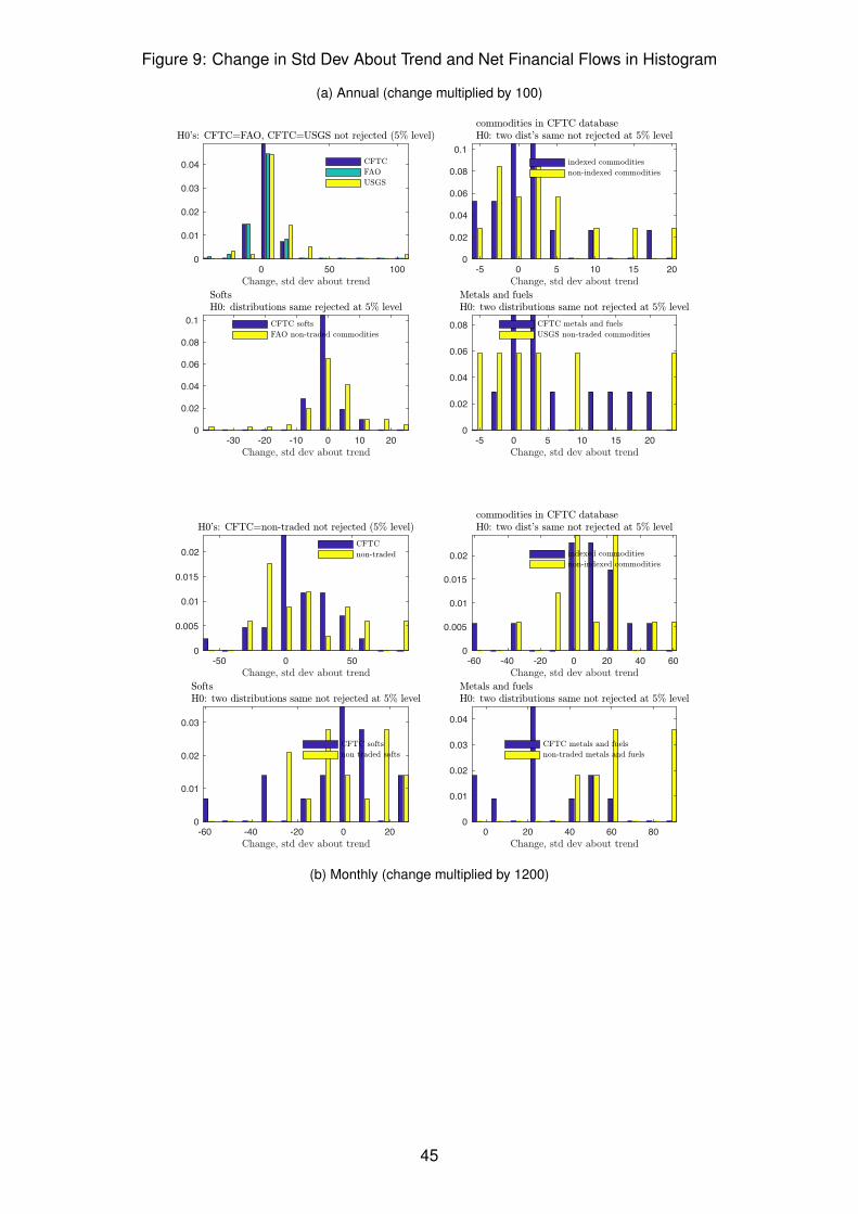
Figure 9: Change in Std Dev About Trend and Net Financial Flows in Histogram

(a) Annual (change multiplied by 100)

0 50 1000

0.01

0.02

0.03

0.04

-5 0 5 10 15 200

0.02

0.04

0.06

0.08

0.1

-30 -20 -10 0 10 200

0.02

0.04

0.06

0.08

0.1

-5 0 5 10 15 200

0.02

0.04

0.06

0.08

-50 0 500

0.005

0.01

0.015

0.02

-60 -40 -20 0 20 40 600

0.005

0.01

0.015

0.02

-60 -40 -20 0 200

0.01

0.02

0.03

0 20 40 60 800

0.01

0.02

0.03

0.04

(b) Monthly (change multiplied by 1200)

45

Figure 10: Volatility and Financialization

(a) Annual Data

0 5 10 15 20 25

100200300

0 10 20 30 40 50 60

100200300

0 5 10 15 20 25

20

40

0 10 20 30 40 50 60

20

40

0 2 4 6

20406080100120

0 5 10 15 20

20406080100120

0 5 10 15 20 25

100200300

0 10 20 30 40 50 60

100200300

(b) Monthly Data

Panel (a): each observation is a price volatility, volume pair for a particular date and commodity. The volatility is the standard deviation of real commodity pricegrowth, expressed in annual percent terms by multiplying by100. The volatility for a particular date is based on a centered plus or minus two year window ofdata on the logarithmic first difference of the commodity price. We use the level of our two measures of volume (scaled by world production), as indicatedin the bottom of the two columns of graphs. Panel (b): same as in Panel , except that to convert the volatility data to annual percent terms we multiply eachvolatility observation by100⇥

p12.

46

Figure 11: Response of Volatility to Volume of Trade

(a) Annual Data

-500 0 500 10000

0.002

0.004

0.006

0.008

0.01

0.012

0.014

0.016

(b) Monthly Data

-100 0 100 200 300 400 5000

0.005

0.01

0.015

0.02

0.025

0.03

0.035

47

Figure 12: Cumulative Returns from 3 Futures Contract Strategies

1970 1975 1980 1985 1990 1995 2000 2005

50

100

150

200

250

Note : (i) hot open interest growth strategy invests in equally weighted basket of commodity futures which have the highest open interest growth in previous period; (ii) hot imbalance strategy is analogous to (i),except commodities are selected based on imbalance, a volume measure that is proportional to net financial flows; (iii) hot random strategy invests in an equally weighted, random set of commodities; (iv)shaded area is 90 percent confidence interval, constructed from 200,000 realizations of the hot, random futures market strategy. For additional details, see text.

Figure 13: Sharpe Ratio for Portfolios

0 0.02 0.04 0.06 0.08 0.1 0.12 0.14 0.160

50

100

150

200

250

300histogram of Sharpe Ratios for random strategy, p-value nff = 0.442, p-value oi = 0.006

48

Figure 14: Histograms of Volatility Drawn from 2

nd and 3

rd Quartiles of Volume

(a) Sorting on Open Interest

0 10 20 30 40 50 600

50

100

150

200

250

300

350

400

(b) Sorting on Net Financial Flows

0 10 20 30 40 50 600

50

100

150

200

250

300

350

49

Figure 15: Impact of Temporal Aggregation on Pairwise Correlations Among Commmodity Futures

1995 2000 2005 2010

0.1

0.2

0.3

0.4

1995 2000 2005 2010

0.1

0.2

0.3

0.4

1995 2000 2005 2010

0.1

0.2

0.3

0.4

0.5

1995 2000 2005 2010

0

0.2

0.4

0.6

50

Figure 16: Correlation, Futures Returns and Stock Returns

(a) Daily Data

1992 1994 1996 1998 2000 2002 2004 2006 2008 2010-0.1

0

0.1

0.2

0.3

0.4

1992 1994 1996 1998 2000 2002 2004 2006 2008 2010

-0.3

-0.2

-0.1

0

0.1

0.2

0.3

0.4

0.5

0.6

(b) Monthly Data

51

Table 1: Annual Spot Prices and World Production for Commodities in CFTC Data

Commodity Commodity in Quantity World production Price Value Sharein CFTC Data and Price Data Source Source Source 1992-2012

Panel (a)oil CRUDE OIL BP BP derived 28.11coal COAL BP BP derived 7.12natural gas NATURAL GAS BP BP derived 9.66propane PROPANE EIA EIA derived 0.86distillate fuel oil HEATING OIL EIA EIA derived 9.54gasoline GASOLINE EIA EIA derived 8.83

Panel (b)gold GOLD USGS USGS derived 1.12silver SILVER USGS USGS derived 0.14copper COPPER USGS USGS derived 1.24platinum PLATINUM USGS USGS derived 0.11aluminum ALUMINUM USGS USGS derived 1.4palladium PALLADIUM USGS USGS derived 0.05

Panel (c)cotton COTTON USDA USDA derived 0.87roundwood LUMBER FAOSTAT FAOSTAT derived 2.6sugar SUGAR USDA Trading Economics derived 1.01pig crop PORK BELLIES USDA FAOSTAT derived 2.61calves CATTLE USDA FAOSTAT derived 4.6rice RICE FAOSTAT FAOSTAT derived 3.43cowmilk BUTTER FAOSTAT derive FAOSTAT 4.65oats OATS FAOSTAT FAOSTAT FAOSTAT 0.1wheat WHEAT FAOSTAT FAOSTAT FAOSTAT 2.88soybeans SOYBEANS FAOSTAT FAOSTAT FAOSTAT 1.3coffee, green COFFEE FAOSTAT FAOSTAT FAOSTAT 0.21cocoabean COCOA FAOSTAT FAOSTAT FAOSTAT 0.1oranges ORANGE JUICE FAOSTAT FAOSTAT FAOSTAT 0.43corn CORN FAOSTAT FAOSTAT FAOSTAT 2.84soybean oil SOYBEAN OIL FAOSTAT USDA derived 0.48soybean meal SOYBEAN MEAL IMF USDA derived 1.09

Notes: (i) Variables in first column are the names of the traded commodities according to the CFTC database; (ii) a variable in the second column is thecommodity for which we have output and price data, and which is closest to the variable in the first column; (iii) sources: BP - British Petroleum, USDA - UnitedStates Department of Agriculture, FAOSTAT - United Nations Food and Agriculture Organization, USGS - United States Geological Survey, EIA - United StatesEnergy Information Administration, IMF - International Monetary Fund, ’derived’ - value derived from other two sources, e.g., a price is derived if it is obtainedfrom the ratio of value to quantity produced; (iv) share - share in world production, sum of shares equals unity; (v) we used ’pig crop’ as a measure of each ofHOGS and PORK BELLIES.

52

Tabl

e2:

Mon

thly

Spo

tPric

esfo

rCom

mod

ities

inC

FTC

Dat

a

Nam

eR

ange

Sou

rce

Des

crip

tion

Cru

de_o

il19

59/1

-201

5/12

Trad

ing

Eco

nom

ics

Coa

l19

80/1

-201

5/12

IMF

Aust

ralia

nth

erm

alco

al,1

2,00

0-bt

u/po

und,

Less

than

1%su

lfur,

14%

ash,

FOB

New

cast

le/P

ortK

embl

a

Nat

ural

_gas

1990

/4-2

015/

12Tr

adin

gE

cono

mic

s

Cot

ton

1959

/6-2

015/

12Tr

adin

gE

cono

mic

s

Sof

tSaw

nwoo

d19

80/1

-201

5/12

IMF

Aver

age

expo

rtpr

ice

ofD

ougl

asFi

r,U

.S.P

rice,

US

$pe

rcub

icm

eter

Sug

ar19

59/1

-201

5/12

Trad

ing

Eco

nom

ics

Sw

ine

(por

k)19

80/1

-201

5/12

IMF

51-5

2%le

anH

ogs,

U.S

.pric

e,U

Sce

nts

perp

ound

.

Bee

f19

80/1

-201

5/12

IMF

Aust

ralia

nan

dN

ewZe

alan

d85

%le

anfo

res,

CIF

U.S

.im

port

pric

e

Ric

e19

81/4

-201

5/12

Trad

ing

Eco

nom

ics

raw

_milk

1959

/1-2

015/

12FR

ED

Pro

duce

rPric

eIn

dex

byC

omm

odity

forF

arm

Pro

duct

s:R

awM

ilk

Oat

1979

/1-2

015/

12Tr

adin

gE

cono

mic

s

Whe

at19

82/3

-201

5/12

Trad

ing

Eco

nom

ics

Soy

bean

s19

59/7

-201

5/12

Trad

ing

Eco

nom

ics

Cof

fee

1972

/7-2

015/

12Tr

adin

gE

cono

mic

s

Coc

oa19

59/7

-201

5/12

Trad

ing

Eco

nom

ics

Ora

nges

1980

/1-2

015/

12IM

FM

isce

llane

ous

oran

ges

CIF

Fren

chim

port

pric

e

Cor

n19

59/1

-201

5/12

Trad

ing

Eco

nom

ics

Gol

d19

68/1

-201

5/12

Trad

ing

Eco

nom

ics

Silv

er19

75/1

-201

5/12

Trad

ing

Eco

nom

ics

Cop

per

1980

/1-2

015/

12IM

FG

rade

Aca

thod

e,LM

Esp

otpr

ice,

CIF

Eur

opea

npo

rts

Pla

tinum

1968

/3-2

015/

12Tr

adin

gE

cono

mic

s

Alu

min

um19

86/3

-201

5/12

Inde

xM

undi

Soy

bean

Oil

1980

/1-2

015/

12IM

FC

hica

goS

oybe

anO

ilFu

ture

s(fi

rstc

ontra

ctfo

rwar

d)

exch

ange

appr

oved

grad

es

prop

ane

1977

/6-2

015/

12FR

ED

Pro

duce

rPric

eIn

dex

byC

omm

odity

forF

uels

and

Rel

ated

Pro

duct

san

dPo

wer

heat

ing_

oil

1986

/6-2

015/

12FR

ED

No.

2H

eatin

gO

ilP

rices

:New

York

Har

bor

gaso

line

1967

/1-2

015/

12FR

ED

Con

sum

erP

rice

Inde

xfo

rAll

Urb

anC

onsu

mer

s:G

asol

ine

(all

type

s)

Palla

dium

1987

/1-2

015/

12Tr

adin

gE

cono

mic

s

Soy

bean

Mea

l19

80/1

-201

5/12

IMF

Chi

cago

Soy

bean

Mea

lFut

ures

(firs

tcon

tract

forw

ard)

Min

imum

48pe

rcen

tpro

tein

53

Tabl

e3:

Mon

thly

Pric

esan

dW

orld

Pro

duct

ion

ofN

on-T

rade

dC

omm

oditi

es

sour

ceof

pric

eda

taD

efini

tion

sour

ceof

prod

uctio

nda

ta

Fish

mea

lIM

FPe

ruFi

shm

eal/p

elle

ts65

%pr

otei

nIn

dexM

undi

,16

bigg

estp

rodu

cerc

ount

ries

Palm

Oil

IMF

Mal

aysi

aPa

lmO

ilIn

dexM

undi

,16

bigg

estp

rodu

cerc

ount

ries

Rub

ber

IMF

Rub

ber,

Sin

gapo

reC

omm

odity

Exc

hang

e,N

o.3

Rub

berS

mok

edS

heet

sFA

OS

TAT

Tea

IMF

Tea,

Mom

basa

,Ken

ya,A

uctio

nP

rice,

From

July

1998

,Ken

yaau

ctio

ns,

Bes

tPek

oeFa

nnin

gs.P

rior,

Lond

onau

ctio

ns,c

.i.f.

U.K

.war

ehou

ses

FAO

STA

T

Ura

nium

IMF

Ura

nium

,NU

EX

CO

,Res

trict

edP

rice

Uni

ted

Nat

ions

Ene

rgy

Sta

tistic

sD

atab

ase

Woo

lTr

adin

gE

cono

mic

sG

reas

yw

ool,

FAO

STA

TB

anan

asIM

FB

anan

as,C

entra

lAm

eric

anan

dE

cuad

or,F

OB

U.S

.Por

tsFA

OS

TAT

Bar

ley

IMF

Can

adia

nno

.1W

este

rnB

arle

yFA

OS

TAT

Rap

esee

dIM

FR

apes

eed

oil,

crud

e,fo

bR

otte

rdam

FAO

STA

TG

roun

dnut

sIM

FG

roun

dnut

s(p

eanu

ts),

40/5

0(4

0to

50co

untp

erou

nce)

,cif

Arg

entin

aFA

OS

TAT

Hid

esIM

FH

ides

,Hea

vyna

tive

stee

rs,o

ver5

3po

unds

,who

lesa

lede

aler

’spr

ice,

Chi

cago

FAO

STA

TIro

nO

reIM

FIro

nO

re,C

hina

impo

rtIro

nO

reFi

nes

62%

FEsp

ot(C

FRTi

anjin

port

)U

SG

STi

nTr

adin

gE

cono

mic

sU

SG

SZi

ncTr

adin

gE

cono

mic

sU

SG

SN

icke

lTr

adin

gE

cono

mic

sU

SG

SLe

adTr

adin

gE

cono

mic

sU

SG

SO

live

Oil

IMF

extra

virg

inle

ssth

an1%

free

fatty

acid

,ex-

tank

erpr

ice

U.K

.In

tern

atio

nalO

live

Cou

ncil

Chi

cken

IMF

Poul

try(c

hick

en),

Who

lebi

rdsp

otpr

ice,

Rea

dy-to

-coo

k,w

hole

,ice

d,G

eorg

iado

cks

FAO

STA

TLa

mb

IMF

Lam

b,fro

zen

carc

ass

Sm

ithfie

ldLo

ndon

FAO

STA

TS

unflo

wer

Oil

IMF

Sun

flow

erO

il,U

Sex

port

pric

efro

mG

ulfo

fMex

ico

FAO

STA

TH

ard

Saw

nwoo

dIM

FH

ard

Saw

nwoo

d,D

ark

Red

Mer

anti,

sele

ctan

dbe

tterq

ualit

yS

awnw

ood

(NC

),FA

OS

TAT

Shr

imp

IMF

Shr

imp,

No.

1sh

ell-o

nhe

adle

ss,2

6-30

coun

tper

poun

d,M

exic

anor

igin

,New

York

port

Fish

erie

san

dA

quac

ultu

reD

epar

tmen

t,U

NS

alm

onIM

FFa

rmB

red

Nor

weg

ian

Sal

mon

,exp

ortp

rice

Fish

erie

san

dA

quac

ultu

reD

epar

tmen

t,U

N

54

Tabl

e4:

Mea

nan

dVo

latil

ityP

rope

rtie

sof

Com

mod

ityP

rice

Gro

wth

(a)A

nnua

l

Com

mod

ityn(i)

Mea

n,sp

otpr

ice

grow

th(⇥

100)

Sta

ndar

dde

viat

ion

(⇥100)

1992

-200

020

01-2

012

diff

(p-v

alue

s(ii)

:the

ory(

iii)

,boo

t)19

92-2

000

2001

-201

2di

ff(p

-val

ues

:the

ory,

boot

)

All

136

-0.6

63.

84.

4(1

0,10

)22

253.

2(8

.6,2

2)

Inde

xed

15-0

.51

6.2

6.7

(12,

12)

1921

2.1

(26,

38)

Non

inde

xed

140.

283.

93.

6(2

0,20

)19

223.

3(7

,16)

Trad

ed29

-0.1

35.

15.

2(1

4,14

)19

222.

6(1

2,26

)

Non

trade

107

-0.8

3.4

4.2

(12,

12)

2226

3.4

(9.1

,21)

(b)M

onth

ly

Com

mod

ityn(iii)

Mea

n(i)

Sta

ndar

dD

evia

tion(

ii)

1992

-200

020

01-2

012

diff

(p-v

alue

s(iv)

:the

ory,

boot

)19

92-2

000

2001

-201

2di

ff(p

-val

ues(

iv)

:the

ory,

boot

)

All

52-1

.55.

16.

6(2

.9,2

.9)

2225

3.2

(7.5

,9)

Inde

xed

15-0

.35

5.6

5.9

(10,

10)

2426

2.9

(15,

18)

Non

inde

xed

14-0

.22

3.8

4(1

7,17

)22

274.

1(3

.1,5

.3)

Trad

ed29

-0.2

94.

75

(11,

11)

2326

3.5

(5.3

,7.5

)

Non

trade

d23

-35.

68.

7(0

.8,0

.83)

2023

2.8

(27,

28)

Not

efo

r(a)

:(i)n

deno

tes

the

num

bero

fcom

mod

ities

inth

esp

ecifi

edgr

oup.

(ii)p

-val

uein

dica

tes

the

prob

abili

ty,u

nder

the

null

hypo

thes

isof

nodi

ffere

nce,

ofge

tting

anev

enhi

gher

diffe

renc

eth

anw

asre

aliz

edin

the

data

.(iii

)p-v

alue

sar

ere

port

edus

ing

apa

rtic

ular

sam

plin

gth

eory

and

bya

boot

stra

ppr

oced

ure

forr

obus

tnes

s(s

eeap

pend

ixfo

rdet

ails

).N

ote

for

(b):

(i)

Mon

thly

log

diffe

renc

eof

spot

pric

es,c

onve

rted

toan

nual

perc

entb

ym

ultip

lyin

gby

1200

;(ii)

Sta

ndar

dde

viat

ion

conv

erte

dto

annu

alpe

rcen

tby

mul

tiply

ing

by10

0⇥p12

;sta

tistic

sap

ply

tost

anda

rdst

anda

rd;(iii)n

deno

tes

the

num

bero

fcom

mod

ities

inth

esp

ecifi

edgr

oup;

(iv)p

-val

uein

dica

tes

the

prob

abili

ty,u

nder

the

null

hypo

thes

isof

nodi

ffere

nce,

ofob

tain

ing

anev

enhi

gher

diffe

renc

eth

anw

asre

aliz

edin

the

data

;the

sam

plin

gth

eory

unde

rlyin

gou

rp-v

alue

sis

base

don

asym

ptot

icth

eory

and

ona

boot

stra

p,as

repo

rted

inth

eap

pend

ix.

55

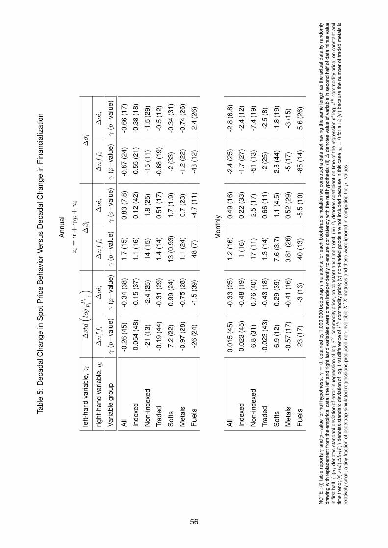
Tabl

e5:

Dec

adal

Cha

nge

inS

potP

rice

Beh

avio

rVer

sus

Dec

adal

Cha

nge

inFi

nanc

ializ

atio

n

Ann

ual

z

i=

↵+�q

i+u

i

left-

hand

varia

ble,

z

i�std

⇣ log

Pi

Pi,�1

⌘��

i��

i

right

-han

dva

riabl

e,q

i�nff

i�oi

i�nff

i�oi

i�nff

i�oi

i

Varia

ble

grou

p�

(p�

valu

e)�

(p�

valu

e)�

(p�

valu

e)�

(p�

valu

e)�

(p�

valu

e)�

(p�

valu

e)

All

-0.2

6(4

5)-0

.34

(38)

1.7

(15)

0.83

(7.8

)-0

.87

(24)

-0.6

6(1

7)

Inde

xed

-0.0

54(4

8)-0

.15

(37)

1.1

(16)

0.12

(42)

-0.5

5(2

1)-0

.38

(18)

Non

-inde

xed

-21

(13)

-2.4

(25)

14(1

5)1.

8(2

5)-1

5(1

1)-1

.5(2

9)

Trad

ed-0

.19

(44)

-0.3

1(2

9)1.

4(1

4)0.

51(1

7)-0

.68

(19)

-0.5

(12)

Sof

ts7.

2(2

2)0.

99(2

4)13

(0.9

3)1.

7(1

.9)

-2(3

3)-0

.34

(31)

Met

als

-0.9

7(2

8)-0

.75

(28)

1.1

(24)

0.7

(23)

-1.2

(22)

-0.7

4(2

6)

Fuel

s-2

6(2

4)-1

.5(3

9)48

(7)

-4.7

(11)

-43

(12)

2.4

(26)

Mon

thly

All

0.01

5(4

5)-0

.33

(25)

1.2

(16)

0.49

(16)

-2.4

(25)

-2.8

(6.8

)

Inde

xed

0.02

3(4

5)-0

.48

(19)

1(1

6)0.

22(3

3)-1

.7(2

7)-2

.4(1

2)

Non

-inde

xed

6.8

(31)

0.76

(40)

17(1

1)2.

5(1

7)-5

1(1

3)-7

.4(1

9)

Trad

ed-0

.023

(43)

-0.4

3(1

8)1.

3(1

4)0.

66(1

1)-2

(25)

-2.5

(8)

Sof

ts6.

9(1

2)0.

29(3

9)7.

6(3

.7)

1.1

(4.5

)2.

3(4

4)-1

.8(1

9)

Met

als

-0.5

7(1

7)-0

.41

(16)

0.81

(26)

0.52

(29)

-5(1

7)-3

(15)

Fuel

s23

(17)

-3(1

3)40

(13)

-5.5

(10)

-85

(14)

5.6

(26)

NO

TE:(

i)ta

ble

repo

rts�

andp�

valu

efo

rnul

lhyp

othe

sis,

�=

0,

obta

ined

by1,

000,

000

boot

stra

psi

mul

atio

ns;f

orea

chbo

otst

rap

sim

ulat

ion

we

cons

truct

ada

tase

thav

ing

the

sam

ele

ngth

asth

eac

tual

data

byra

ndom

lydr

awin

gw

ithre

plac

emen

tfro

mth

eem

piric

alda

ta;t

hele

ftan

drig

htha

ndva

riabl

esw

ere

draw

nin

depe

nden

tlyto

ensu

reco

nsis

tenc

yw

ithth

enu

llhy

poth

esis

;(ii)�

deno

tes

valu

eof

varia

ble

inse

cond

half

ofda

tam

inus

valu

ein

first

half;

(iii)�

i

deno

tes

stan

dard

devi

atio

nof

erro

rin

regr

essi

onof

log,

ith

com

mod

itypr

ice,

onco

nsta

ntan

dtim

etre

nd;(

iv)�

i

deno

tes

coef

ficie

nton

time

ofth

ere

gres

sion

oflo

g,ith

com

mod

itypr

ice,

onco

nsta

ntan

dtim

etre

nd;(

v)std(�

logPi

)de

note

sst

anda

rdde

viat

ion

oflo

g,fir

stdi

ffere

nce

ofith

com

mod

itypr

ice;

(v)n

on-tr

aded

good

sar

eno

tinc

lude

dbe

caus

ein

this

case

q i=

0fo

ralli;

(vi)

beca

use

the

num

bero

ftra

ded

met

als

isre

lativ

ely

smal

l,a

tiny

fract

ion

ofbo

otst

rap-

sim

ulat

edre

gres

sion

spr

oduc

edno

n-in

vert

ible

X0 X

mat

rices

and

thes

ew

ere

igno

red

inco

mpu

ting

thep�

valu

es.

56

Table 6: Regression, Volatility of Spot Price Growth on Volume of Futures Trades1

(a) Annual

volatilityt = constant+ � ⇥ volumet

Variables Net Financial Flows Open Interest

All-0.55 -0.24

(-0.71,-0.072) (-0.33,-0.07)

Traded-0.42 -0.16

(-0.55,0.097) (-0.24,0.043)

Softs-0.41 -0.034

(-1.7,0.73) (-0.42,0.15)

Metals & Fuels-0.64 -0.31

(-0.85,-0.14) (-0.4,-0.088)

(b) Monthly

volatilityt = constant+ � ⇥ volumet

Variables Net Financial Flows Open Interest

All-0.13 -0.058

(-0.25,-0.052) (-0.12,-0.02)

Traded-0.26 -0.17

(-0.36,-0.15) (-0.22,-0.11)

Softs0.28 0.079

(-0.25,0.35) (-0.11,0.14)

Metals & Fuels-0.18 -0.099

(-0.3,-0.082) (-0.15,-0.043)

Notes: (1) the table reports our least squares estimates of �, the (common) slope coefficient in a regression of volatility (a two-year moving, centered standarddeviation of one-period real spot price growth) on our two measures of volume (net financial flows and open interest); in all cases, the standard deviation ismultiplied by 100 to convert to percent terms, and in the case of monthly data, the standard deviations are in addition multiplied by

p12 to convert to annual

units; (2) numbers not in parentheses are the least squares estimate value of �; (3) numbers in parentheses are the boundaries of 95 percent intervals,computed using 5,000 bootstrap simulations under the null hypothesis that the left and right-side variables are independent; (4) in each simulation: (i) thecommodity price growth and volume data were sampled independently with replacement from the actual data, (ii) the volatility data were computed by applyingthe centered moving window procedure to the artificial commodity price growth data, and (iii) the regression performed on the actual data was computed onthe artificial data; (5) “All” means the analysis is done using all commodities, “traded” means only commodities in our CFTC data included in the analysis;”softs” and “metals & fuels” means only commodities classified as softs and metals and fuels included in the analysis (see text for further discussion).

57

Table 7: Futures Returns and Financialization

correlationt = c+ � ⇥ volumet

Correlation of Futures Returns with:Equity Returns 3 month T-bill

Measure of Volume Monthly Daily Monthly Daily

Net financial flows3.6 4 0.88 0.17

(-2.7,2.8) (-4.6,11) (-1.9,2.5) (-0.3,0.54)

Open interest1 1.4 1.1 0.25

(-1.7,2.1) (-5,5.7) (-0.94,1.3) (-0.19,0.28)

volatilityt = c+ � ⇥ volumet

Volatility of Futures ReturnsMeasure of Volume Monthly Daily

Net financial flows-0.065 0.0014

(-0.29,0.38) (-0.049,0.058)

Open interest-0.11 -0.004

(-0.15,0.28) (-0.02,0.049)

Notes: see text for a discussion of estimates of �, which are the number not in parentheses. Numbers in parentheses are 95 confidence intervals under thenull hypothesis, � = 0.

58

1

Working Paper Series

A series of research studies on regional economic issues relating to the Seventh Federal Reserve District, and on financial and economic topics.

The Effects of the Massachusetts Health Reform on Financial Distress WP-14-01 Bhashkar Mazumder and Sarah Miller Can Intangible Capital Explain Cyclical Movements in the Labor Wedge? WP-14-02 François Gourio and Leena Rudanko Early Public Banks WP-14-03 William Roberds and François R. Velde Mandatory Disclosure and Financial Contagion WP-14-04 Fernando Alvarez and Gadi Barlevy The Stock of External Sovereign Debt: Can We Take the Data at ‘Face Value’? WP-14-05 Daniel A. Dias, Christine Richmond, and Mark L. J. Wright Interpreting the Pari Passu Clause in Sovereign Bond Contracts: It’s All Hebrew (and Aramaic) to Me WP-14-06 Mark L. J. Wright AIG in Hindsight WP-14-07 Robert McDonald and Anna Paulson On the Structural Interpretation of the Smets-Wouters “Risk Premium” Shock WP-14-08 Jonas D.M. Fisher Human Capital Risk, Contract Enforcement, and the Macroeconomy WP-14-09 Tom Krebs, Moritz Kuhn, and Mark L. J. Wright Adverse Selection, Risk Sharing and Business Cycles WP-14-10 Marcelo Veracierto Core and ‘Crust’: Consumer Prices and the Term Structure of Interest Rates WP-14-11 Andrea Ajello, Luca Benzoni, and Olena Chyruk

The Evolution of Comparative Advantage: Measurement and Implications WP-14-12 Andrei A. Levchenko and Jing Zhang Saving Europe?: The Unpleasant Arithmetic of Fiscal Austerity in Integrated Economies WP-14-13 Enrique G. Mendoza, Linda L. Tesar, and Jing Zhang Liquidity Traps and Monetary Policy: Managing a Credit Crunch WP-14-14 Francisco Buera and Juan Pablo Nicolini

2

Working Paper Series (continued) Quantitative Easing in Joseph’s Egypt with Keynesian Producers WP-14-15 Jeffrey R. Campbell Constrained Discretion and Central Bank Transparency WP-14-16 Francesco Bianchi and Leonardo Melosi Escaping the Great Recession WP-14-17 Francesco Bianchi and Leonardo Melosi More on Middlemen: Equilibrium Entry and Efficiency in Intermediated Markets WP-14-18 Ed Nosal, Yuet-Yee Wong, and Randall Wright Preventing Bank Runs WP-14-19 David Andolfatto, Ed Nosal, and Bruno Sultanum The Impact of Chicago’s Small High School Initiative WP-14-20 Lisa Barrow, Diane Whitmore Schanzenbach, and Amy Claessens Credit Supply and the Housing Boom WP-14-21 Alejandro Justiniano, Giorgio E. Primiceri, and Andrea Tambalotti The Effect of Vehicle Fuel Economy Standards on Technology Adoption WP-14-22 Thomas Klier and Joshua Linn What Drives Bank Funding Spreads? WP-14-23 Thomas B. King and Kurt F. Lewis Inflation Uncertainty and Disagreement in Bond Risk Premia WP-14-24 Stefania D’Amico and Athanasios Orphanides Access to Refinancing and Mortgage Interest Rates: WP-14-25 HARPing on the Importance of Competition Gene Amromin and Caitlin Kearns Private Takings WP-14-26 Alessandro Marchesiani and Ed Nosal Momentum Trading, Return Chasing, and Predictable Crashes WP-14-27 Benjamin Chabot, Eric Ghysels, and Ravi Jagannathan Early Life Environment and Racial Inequality in Education and Earnings in the United States WP-14-28 Kenneth Y. Chay, Jonathan Guryan, and Bhashkar Mazumder Poor (Wo)man’s Bootstrap WP-15-01 Bo E. Honoré and Luojia Hu

Revisiting the Role of Home Production in Life-Cycle Labor Supply WP-15-02 R. Jason Faberman

3

Working Paper Series (continued) Risk Management for Monetary Policy Near the Zero Lower Bound WP-15-03 Charles Evans, Jonas Fisher, François Gourio, and Spencer Krane Estimating the Intergenerational Elasticity and Rank Association in the US: Overcoming the Current Limitations of Tax Data WP-15-04 Bhashkar Mazumder External and Public Debt Crises WP-15-05 Cristina Arellano, Andrew Atkeson, and Mark Wright The Value and Risk of Human Capital WP-15-06 Luca Benzoni and Olena Chyruk Simpler Bootstrap Estimation of the Asymptotic Variance of U-statistic Based Estimators WP-15-07 Bo E. Honoré and Luojia Hu Bad Investments and Missed Opportunities? Postwar Capital Flows to Asia and Latin America WP-15-08 Lee E. Ohanian, Paulina Restrepo-Echavarria, and Mark L. J. Wright Backtesting Systemic Risk Measures During Historical Bank Runs WP-15-09 Christian Brownlees, Ben Chabot, Eric Ghysels, and Christopher Kurz What Does Anticipated Monetary Policy Do? WP-15-10 Stefania D’Amico and Thomas B. King Firm Entry and Macroeconomic Dynamics: A State-level Analysis WP-16-01 François Gourio, Todd Messer, and Michael Siemer Measuring Interest Rate Risk in the Life Insurance Sector: the U.S. and the U.K. WP-16-02 Daniel Hartley, Anna Paulson, and Richard J. Rosen Allocating Effort and Talent in Professional Labor Markets WP-16-03 Gadi Barlevy and Derek Neal The Life Insurance Industry and Systemic Risk: A Bond Market Perspective WP-16-04 Anna Paulson and Richard Rosen Forecasting Economic Activity with Mixed Frequency Bayesian VARs WP-16-05 Scott A. Brave, R. Andrew Butters, and Alejandro Justiniano Optimal Monetary Policy in an Open Emerging Market Economy WP-16-06 Tara Iyer Forward Guidance and Macroeconomic Outcomes Since the Financial Crisis WP-16-07 Jeffrey R. Campbell, Jonas D. M. Fisher, Alejandro Justiniano, and Leonardo Melosi

4

Working Paper Series (continued) Insurance in Human Capital Models with Limited Enforcement WP-16-08 Tom Krebs, Moritz Kuhn, and Mark Wright Accounting for Central Neighborhood Change, 1980-2010 WP-16-09 Nathaniel Baum-Snow and Daniel Hartley The Effect of the Patient Protection and Affordable Care Act Medicaid Expansions on Financial Wellbeing WP-16-10 Luojia Hu, Robert Kaestner, Bhashkar Mazumder, Sarah Miller, and Ashley Wong The Interplay Between Financial Conditions and Monetary Policy Shock WP-16-11 Marco Bassetto, Luca Benzoni, and Trevor Serrao Tax Credits and the Debt Position of US Households WP-16-12 Leslie McGranahan The Global Diffusion of Ideas WP-16-13 Francisco J. Buera and Ezra Oberfield Signaling Effects of Monetary Policy WP-16-14 Leonardo Melosi Constrained Discretion and Central Bank Transparency WP-16-15 Francesco Bianchi and Leonardo Melosi Escaping the Great Recession WP-16-16 Francesco Bianchi and Leonardo Melosi The Role of Selective High Schools in Equalizing Educational Outcomes: Heterogeneous Effects by Neighborhood Socioeconomic Status WP-16-17 Lisa Barrow, Lauren Sartain, and Marisa de la Torre Monetary Policy and Durable Goods WP-16-18 Robert B. Barsky, Christoph E. Boehm, Christopher L. House, and Miles S. Kimball Interest Rates or Haircuts? Prices Versus Quantities in the Market for Collateralized Risky Loans WP-16-19 Robert Barsky, Theodore Bogusz, and Matthew Easton Evidence on the within-industry agglomeration of R&D, production, and administrative occupations WP-16-20 Benjamin Goldman, Thomas Klier, and Thomas Walstrum Expectation and Duration at the Effective Lower Bound WP-16-21 Thomas B. King

5

Working Paper Series (continued) The Term Structure and Inflation Uncertainty WP-16-22 Tomas Breach, Stefania D’Amico, and Athanasios Orphanides The Federal Reserve’s Evolving Monetary Policy Implementation Framework: 1914-1923 WP-17-01 Benjamin Chabot Neighborhood Choices, Neighborhood Effects and Housing Vouchers WP-17-02 Morris A. Davis, Jesse Gregory, Daniel A. Hartley, and Kegon T. K. Tan Wage Shocks and the Technological Substitution of Low-Wage Jobs WP-17-03 Daniel Aaronson and Brian J. Phelan Worker Betas: Five Facts about Systematic Earnings Risk WP-17-04 Fatih Guvenen, Sam Schulhofer-Wohl, Jae Song, and Motohiro Yogo The Decline in Intergenerational Mobility After 1980 WP-17-05 Jonathan Davis and Bhashkar Mazumder Is Inflation Default? The Role of Information in Debt Crises WP-17-06 Marco Bassetto and Carlo Galli Does Physician Pay Affect Procedure Choice and Patient Health? Evidence from Medicaid C-section Use WP-17-07 Diane Alexander Just What the Nurse Practitioner Ordered: Independent Prescriptive Authority and Population Mental Health WP-17-08 Diane Alexander and Molly Schnell How do Doctors Respond to Incentives? Unintended Consequences of Paying Doctors to Reduce Costs WP-17-09 Diane Alexander Closing the Gap: The Impact of the Medicaid Primary Care Rate Increase on Access and Health Unintended Consequences of Paying Doctors to Reduce Costs WP-17-10 Diane Alexander and Molly Schnell Check Up Before You Check Out: Retail Clinics and Emergency Room Use WP-17-11 Diane Alexander, Janet Currie, and Molly Schnell The Effects of the 1930s HOLC “Redlining” Maps WP-17-12 Daniel Aaronson, Daniel Hartley, and Bhashkar Mazumder Inflation at the Household Level WP-17-13 Greg Kaplan and Sam Schulhofer-Wohl

6

Working Paper Series (continued) The Effect of Fertility on Mothers’ Labor Supply over the Last Two Centuries WP-17-14 Daniel Aaronson, Rajeev Dehejia, Andrew Jordan, Cristian Pop-Eleches, Cyrus Samii, and Karl Schulze Financialization in Commodity Markets WP-17-15 VV Chari and Lawrence J. Christiano