financial markets and politics- studying the effect of
TRANSCRIPT

Thesis Toni Joe Lebbos
1
Financial Markets and Politics- Studying the effect of Policy Risk on Stock Market Volatility in France 1967-2015
Toni Joe Lebbos
201401016
Thesis Final Draft

Thesis Toni Joe Lebbos
2
TABLE OF CONTENTS ABSTRACT .......................................................................................... 5
1 INTRODUCTION ............................................................................. 6
2 LITERATURE REVIEW .................................................................. 7 2.1 DEFINITIONS .................................................................................................. 8 2.2 RELEVANT STUDIES ...................................................................................... 12
3 DATA .............................................................................................. 16 DATA ON STOCK MARKET PRICES AND VOLATILITY .......................................... 17 INFLATION AND GDP PER CAPITA ..................................................................... 20 HISTORICAL DATA ON THE FRENCH GOVERNMENT ............................................ 20
a) Election years .................................................................................. 21 b) Cohesiveness and Distance ................................................................ 21 c) Sociocultural Mood ........................................................................... 23
4 EMPIRICAL ESTIMATION ........................................................... 24
5 RESULTS ......................................................................................... 25
6 DISCUSSION ................................................................................... 28
7 ROBUSTNESS CHECKS ................................................................ 30 6.1 TESTING FOR OMITTED VARIABLE BIAS ....................................................... 30 6.2 TESTING FOR AUTOCORRELATION ................................................................ 30 6.3 TESTING FOR MULTICOLLINEARITY .............................................................. 35 6.4 EXCLUDING ABNORMAL OBSERVATION FROM SAMPLE ................................... 38 ACCOUNTING FOR CRISIS YEARS USING DUMMY VARIABLES .............................. 40 ANALYSIS USING DIFFERENT DEFINITION OF VOLATILITY .................................. 43
8 LIMITATIONS ................................................................................ 46
9 CONCLUSION ................................................................................. 47
BIBLIOGRAPHY ............................................................................... 49
ANNEXES .......................................................................................... 52 ANNEX 1: MODEL 1 & 2 OUTPUT EXCLUDING MAIN EXPLANATORY VARIABLES 52

Thesis Toni Joe Lebbos
3
ANNEX 2: MODEL 1 OUTPUT .............................................................................. 53 ANNEX 3: MODEL 2 OUTPUT .............................................................................. 53 ANNEX 3: STANDARD DURBIN WATSON D-STATISTIC MODEL 1 & 2 ................... 54 ANNEX 4: CORRGRAM OUTPUT MODEL 1 & 2 .................................................... 54 ANNEX 5: MULTICOLLINEARITY TEST ................................................................ 55 ANNEX 6: OUTPUT MODEL 1 ADJUSTED FOR MULTICOLLINEARITY .................... 56 ANNEX 7: OUTPUT MODEL 2 ADJUSTED FOR MULTICOLLINEARITY .................... 56 ANNEX 8: OUTPUT MODEL 1 WITH OMISSION OF ABNORMAL OBSERVATIONS ...... 57 ANNEX 9: OUTPUT MODEL 2 WITH OMISSION OF ABNORMAL OBSERVATIONS ...... 57 ANNEX 10: OUTPUT MODEL 1 WITH ACCOUNTING FOR CRISIS YEARS ................ 58 ANNEX 11: OUTPUT MODEL 2 WITH ACCOUNTING FOR CRISIS YEARS ................ 58 ANNEX 12: OUTPUT MODEL 1 USING METHOD 2 ................................................. 59 ANNEX 13: OUTPUT MODEL 2 USING METHOD 2 ................................................. 59 ANNEX 14: MODELS 1 & 2 WITH INTEREST INCLUDED AS EXPLANATORY
VARIABLE .......................................................................................................... 60
Table 1 Summary of Definitions .......................................................................... 11 Table 2 Main Theories Summary ......................................................................... 13 Table 3 Other relevant studies Summary ............................................................ 15 Table 4 Characteristics of Studies Reviewed ........................................................ 16 Table 5: Descriptive Statistics Volatility ............................................................. 19 Table 6: Model 1 Results ...................................................................................... 26 Table 7: Model 2 Results ...................................................................................... 27 Table 8: Model 1 Adjusted for Multicollinearity .................................................. 35 Table 9: Model 2 Adjusted for Multicollinearity .................................................. 36 Table 10: Model 1 Adjusted for Abnormal Abservations ..................................... 38 Table 11: Model 2 Adjusted for Abnormal Observations ..................................... 39 Table 12: Model 1 with Accounting for Crisis Years ........................................... 41 Table 13: Model 2 with Accounting for Crisis ...................................................... 42 Table 14: Model 1 Using Method 2 ...................................................................... 44 Table 15: Model 2 Using Method 2 ...................................................................... 45

Thesis Toni Joe Lebbos
4
Figure 1: Relationship between political institutions in France under the 5th Republic……………………………………………………………………………………………………………………………9 Figure 2: Political Scenarios In France ................................................................ 11 Figure 3: Box Plot Volatility ............................................................................... 18 Figure 4: Histogram Volatility ............................................................................. 18 Figure 5: Scatter Plot ........................................................................................... 20 Figure 6: Line GRaph R1 ..................................................................................... 31 Figure 7: Line Graph R2 ...................................................................................... 32 Figure 8: Autocorrelation of R1 ........................................................................... 33 Figure 9: Autocorrelation of R2 ........................................................................... 33 Figure 10: Cumulative Periodogram White-Noise Test R1 .................................. 34 Figure 11Cumulative Periodogram White-Noise Test r2 ..................................... 34

Thesis Toni Joe Lebbos
5
ABSTRACT This study examines the impact of having a divided government (as opposed to a unified government) on stock market volatility in France. The role the French government plays throughout the different industries operating on its land is undoubtedly significant as it is through the government that laws and regulations are shaped and implemented. The main theory this paper aims to test empirically relates to the relationship between repartitions of governmental powers and policy risk. According to some literature, a divided government, due to what is referred to as a gridlock effect is less likely to implement policy changes and therefore policy risk is lower. As policy risk is lower, stock market volatility and returns are expected to be lower as well. The intuition behind this theory will be tested by firstly identifying the French government’s status (divided vs. unified) throughout the period spanning from 1967 till 2015, and then paralleling those results with the volatility of stock market returns the various periods considered. I find positive and significant results indicating a higher volatility in times of divided government thus refuting the gridlock theory. These findings are in line with the standard balancing model (Fiorina, 1992) and Mayhew’s Divided We Govern hypothesis. Results remain robust after being subjected to tests for omitted variable bias, autocorrelation, multicollinearty and omission of abnormal observations.
Key Words: Policy Risk, Stock Market Returns, Government, Gridlock JEL-Codes: P16

Thesis Toni Joe Lebbos
6
DIVIDED THEY RISE: STUDYING THE EFFECT OF POLICY RISK ON STOCK MARKET RETURN
1 INTRODUCTION The role a government plays throughout the different industries operating
in a certain country is undoubtedly significant as it is through the government
that laws and regulations are shaped and implemented. These same laws and
regulations ultimately end up shaping pivotal components of the environment
businesses operate on. The ease at which proposed laws are actually translated to
effective, and implemented, laws is vital to company risk assessments. This
brings about an important notion that is often brought up in institutional
economics, finance and political economy and it is the notion of Policy Risk (also
referred to sometimes as Political risk). Policy risk involves the risk that an
investment's returns could be negatively affected as a result of changes in policies
in a given country. The pertinence of this topic is mainly twofold: First, this
topic fills a gap in the literature. Given the research I have conducted, and to the
best of my knowledge, there are no other studies looking at the effect of policy
risk on stock market volatility and returns aside from a study conducted in
Germany (Bechtel & Fuss, 2008). Secondly, with increasing discussions about the
role a government should play in shaping the economy, the relationship between
stock market return and probability of policy change has become an important
academic predicament. In fact, the effect of politics and more specifically policy
risk on stock markets is a topic that is highly discussed in literature today. The
aim of this study is therefore to address two key questions: Is the probability of
nationwide policy change (indicator of policy risk) different under a unified

Thesis Toni Joe Lebbos
7
government as opposed to a divided government? If so, how does this affect
financial markets, and more specifically, stock market volatility? I use data on
stock market returns and political indicators in France from 1967 till 2015 and
estimate the impact of having a divided government using a standard OLS
regression model. Results show a positive and significant between divided states
of the government and higher volatility thus refuting the gridlock theory. Such
results further support Fiorina’s standard balancing model (Fiorina, 1992) and
Mayhew’s (1991) Divided We Govern hypothesis.
Besides this introductory section, this paper is structured as follows:
Chapter 2 presents the literature review where Relevant Definitions are discussed
and the main theories in the literature are elaborated on and discussed. Chapter
3 introduces the data used in this study and specifies its sources. In chapter 4 an
overview of the empirical estimation process is presented and the models used for
the estimation process are elaborated on. Chapter 5 contains results of the
estimation process and chapter 6 discusses various robustness checks conducted
to validate findings. Finally chapter 7 elaborates on the findings and their
significance before concluding in chapter 8.
2 LITERATURE REVIEW
The literature review will start by discussing some key definitions that are
vital to well understanding the topic at hand. Then, the main theories and
models in the literature related to the research question are elaborated on and
the contributions they bring to the study are examined.

Thesis Toni Joe Lebbos
8
2.1 DEFINITIONS
It is fundamental to well define certain term, concepts and notation that
will be used throughout this study. Doing so not only contributes to a better
understanding of the key models and theories but also adds credibility to the
study in that the terms defined usually are backed up by extensive literature.
To start with, it is vital to define terms related to the political system in
France and it’s power repartition. France is a republic, i.e. the institutions
governing France are described by the Constitution, and to be more specific by
the current constitution under the Fifth Republic. The Fifth Republic was
established in 1958, and was largely attributed to the work of General de Gaulle,
and his prime minister at that time Michel Debré. The constitution has been
amended seventeen times since then. Even though the French constitution is
considered parliamentary, one distinction it has is that it allocated relatively
extensive powers to the executive (President and Ministers) when compared to
other western democracies. The executive powers lie mostly within the President
(elected by universal suffrage)’s will. The legislative branch on the other hand
involves mainly the French parliament that is made up of two houses or
chambers. The lower and principal house of parliament is the Assemblée
nationale, or national assembly; the second chamber is the Sénat or Senate. New
bills (projets de loi), proposed by government, and new private members bills
(propositions de loi) must be approved by both chambers, before becoming law
(Francais, Gouvernement.fr, 2015). The figure below provides a clear overview of
the different mechanisms governing institutions in the French political system:

Thesis Toni Joe Lebbos
9
Note: Dotted arrows designate indirect influence whereas the solid ones refer to direct influence through appointment,
voting, regulation, lawsuits and censure) (Wikipedia, 2016)
Another aspect that singularizes the French Fifth Republic from other
Western Political system such as that of the US is the presence of a dual
executive. Through a constitutional arrangement known as semi-presidential
(premier-presidential), the president and a prime minister hold equivalent
rightfulness and legitimacy in their corresponding domains. The president
typically acts as a mediator for establishments of the republic and often is in
FIGURE 1: RELATIONSHIP BETWEEN POLITICAL INSTITUTIONS IN FRANCE UNDER THE 5TH REPUBLIC

Thesis Toni Joe Lebbos
10
charge of decisions related to foreign affairs. The prime minister on the other
hand leads the government and guides the lawmaking process (Baumgartner,
Brouard, Grossman, Lazardeux, & Moody, 2014).
It is also quite relevant to touch upon the definition of a divided
government and that of a unified one. According to Menefee (1991) a divided
government is defined as one where a partisan conflict exists between the
executive and the legislative branches. Tautologically, a unified government is a
government where there is no partisan conflict between the executive and the
legislative branches. In France, whether a government is divided or not goes
beyond a simple binomial system. This is mainly because France has found itself
throughout the years in times where the President and the Prime Minister are
partisan rivals. This type of divided government is referred to as cohabitation
where the executive branch of the government is divided. This, for instance
cannot occur in the United States where the executive cannot be divided. The
only certain alignment of position is that of the National Assembly and the
Prime Minister who always belong to the same partisan camp (Baumgartner et
al, 2014). In short, both the legislative and the executive segments of the French
government might be in a unified or divided state leading to four possible
situations (Siaroff, 2003):

Thesis Toni Joe Lebbos
11
FIGURE 2: POLITICAL SCENARIOS IN FRANCE
Policy risk (also sometimes referred to as political risk) is defined in
various interrelated manners in the literature. For the purpose of this research,
the definition adopted will be that of Carlson (1969), Greene (1974), Aliber
(1975), Baglini (1976) and Lloyd (1976) who, either explicitly or implicitly, define
political policy risk to be the risk that the returns on an investment incur losses
due to shift in political policies shaping business environment (Kobrin, 1982).
This includes instabilities in investment returns sourcing from changes in
government structure.
TABLE 1 SUMMARY OF DEFINITIONS
Term Definition Source Divided Government
Government where a partisan conflict exists between the executive and the legislative branches
Menefee (1991)
Unified Government
Government where there is no partisan conflict between the executive and the legislative branches
Menefee (1991)
Policy Risk Risk that the returns on an investment incur losses due to shift in political policies shaping business environment. This includes instabilities in investment returns sourcing from changes in government structure
Carlson (1969), Greene (1974), Aliber (1975), Baglini (1976) and Lloyd (1976)
Devided Legislature/
Divided Executive
Unified Legislature/
Divided Executive
Devided Legislature/
Unified Executive
Unified Legislature/
Unified Executive

Thesis Toni Joe Lebbos
12
Fifth Republic
The fifth republic was established in 1958, and was largely the work of General de Gaulle, and Michel Debré his prime minister. It has been amended 17 times.
French Government Website
Assemblée Nationale
The lower and principal house of parliament French Government Website
Sénat The Senate French Government Website
2.2 RELEVANT STUDIES
The main purpose behind this paper progresses around verifying or
negating empirically the notion that with a divided government, policy changes
are less likely to be implemented because of a certain “gridlock” effect. The
gridlock effect, in theory, is supposed to assuage risk by increasing the
predictability of future economic policies under the claim that it is hard for
government to implement law under divided governments. A lower level of policy
risk is therefore expected under divided governments. In the context of this
study, stock market return volatility will serve as an indicator or measure of risk;
i.e. volatility of returns should be lower under divided governments. This theory
is firstly backed up by Fowler (2006) who argues that a divided government
assuages policy risk by reducing uncertainties related to large policy changes
because a divided government obliges the opposing parties to confer and limits
the range of policy changes that would be possible under a unified government
(Fowler, 2006). Bechtel and Fuss (2008) also back up this theory empirically in
that they argue as well that a divided government in Germany entails less policy
risk: “financial markets can operate under lower policy risk in times of divided
than in periods of unified governments” (Bechtel & Fuss, 2008, p. 1). Likewise, a
more recent paper by Kim, Pantzalis and Park (2012) published in the Journal of

Thesis Toni Joe Lebbos
13
Financial Economics also argues for this rational stating that “uncertainty
regarding the impact of future policies on forms rises with the difficulty in
assessing the set of preferred policies” (Kim et al, 2012, p. 2).
Also, since most of the policy risk surges from law production and
implementation, looking at literature related to that is quite important and
useful. Baumgartner et al. (2014) look at differences in law production in France
under diverse government power repartitions (divided vs. unified). They do not
find any significant difference in changes of overall legislative productivity.
Conley (2007), who runs a study on France, finds on the other hand that major
shifts in the political landscape have happened in periods of divided government.
He clearly states:
“The Constitution of the Fifth Republic was established to avoid legislative
paralysis, and the French presidents’ misgivings about the majority’s policies
notwithstanding, considerable policy shifts—from the social realm to
denationalizations—have been the result of divided government in the last two
decades. Parliament’s responsibility for such policy changes is clear” (Conley,
2007, p. 258)
Mayhew, in Divided We Govern, disputes the formerly “conventional”
notion that under divided governments in the US (when Congress and the
presidency are controlled by different parties) less important legislation is passed
than under unified government (Mayhew, 1991). TABLE 2 MAIN THEORIES SUMMARY
Authors Publication Insight Fowler (2006) Elections and Markets: The Divided government assuages policy risk by

Thesis Toni Joe Lebbos
14
Effect of Partisanship, Policy Risk, and Electoral Margins on the Economy
reducing uncertainties related to large policy changes because a divided government obliges the opposing parties to confer and limits the range of policy changes that would be possible under a unified government
Bechtel and Fuss (2008)
When Investors Enjoy Less Policy Risk: Divided Government, Economic Policy Change, and Stock Market Volatility, 1970-2005
“Financial markets can operate under lower policy risk in times of divided than in periods of unified governments” (Bechtel & Fuss, 2008)
Kim, Pantzalis and Park (2012)
Political Geography and Stock Returns: The Value and Risk Implications of Proximity to Political Power
“Uncertainty regarding the impact of future policies on forms rises with the difficulty in assessing the set of preferred policies” (Kim, Pantzalis, & Park, 2012).
Baumgartner et al. (2014)
Divided Government, Legislative Productivity, and Policy Change in the USA and France
No significant difference in changes of overall legislative productivity under Divided vs. Unified Government
Conley (2007) Presidential Republics and Divided Government: Law-Making and Executive Politics in the United States and France
Major shifts in the French political landscape have happened under divided governments.
Mayhew (1991) Divide We Govern There should be no difference in legislative productivity under divided vs. unified government
Moreover, some other relevant studies provide important insight as well.
Alesina and Rosenthal (1995) for instance look into the impact of divided
government on key economic parameters such as growth and inflation. They find
that variations in economic growth are correlated with election results and,
conversely, electoral results tend to depend on the state of the economy. Karol
(2000) finds that conflict of the executive and the legislative branches influences
trade. Poterba (1994) finds that budget deficit reduction in the U.S. states is
lower under divided than under unified government and Roubini and Sachs
(1989) conclude that unified governments “respond more (and more quickly) to

Thesis Toni Joe Lebbos
15
income shocks” (Roubini & J, 1989, p. 823). Milner and Rosendorff (1997)
conjecture that international trade agreements are less likely to be ratified under
divided government. The evidence suggests that the level of non-tariff barriers
significantly increases if there is partisan conflict between Congress and the
President (Lohmann & O’Halloran, 1994). Howell et al. (2000) estimates that
“periods of divided government depress the production of landmark legislation by
about 30%, at least when productivity is measured on the basis of
contemporaneous perceptions of important legislation. Lastly, Fowler (2006) finds
that inflation risk is significantly lower in the U.S. if the party of the president
does not control the majority in Congress.
TABLE 3 OTHER RELEVANT STUDIES SUMMARY
Authors Insight Kim, Pantzalis and Park, 2008
Impact of political proximity (geographical proximity as well as political connections of companies to the government) on stock market returns
Alenisa & Rosenthal, 1995
Impact of divided government on key economic parameters such as growth and inflation
Karol, 2000 Conflict of the executive and the legislative branches influences trade Poterba, 1994 Budget deficit reduction in the U.S. states is lower under divided than
under unified government Roubini & J, 1989 Unified governments “respond more (and more quickly) to income shocks Milner & Rosendorff, 1996
International trade agreements are less likely to be ratified under divided government
Lohmann & O’Halloran, 1994
Level of non-tariff barriers significantly increases if there is partisan conflict between Congress and the President
Howell, Adler, Cameron, & Riemann, 2000
Periods of divided government depress the production of landmark legislation by about 30%, at least when productivity is measured on the basis of contemporaneous perceptions of important legislation
Fowler, 2006 Inflation risk is significantly lower in the U.S. if the party of the president does not control the majority in Congress
Finally, when it comes to literature that has contributed to the
methodological aspect of this paper, it is vital to mention three core models. The

Thesis Toni Joe Lebbos
16
first is a paper by Kim, Pantzalis and Park (2012) where the authors discuss the
impact of political proximity (geographical proximity as well as political
connections of companies to the government) on stock market returns (Kim et al,
2012). The second paper is by a paper authored by Bechtel and Fuss entitled. In
this study, the authors focus more on defining policy risk, and studying its
impact on stock market returns given different government compositions (Bechtel
& Fuss, 2008). And finally, a paper by Baumgartner et al (2014) assesses the
variations in law production under different states of the government by
regressing that latter variable onto dummy variables depicting the status of the
French government. Table 4 below summarizes the main studies considered
when developing the empirical estimation of this paper:
TABLE 4 CHARACTERISTICS OF STUDIES REVIEWED
Authors Country Data collection Analysis Kim, Pantzalis, & Park (2012)
United States Taylor’s Encyclopedia of Government Officials: Federal and State” and “State Elective Officials and the Legislatures U.S. Census Bureau Dave Leip’s Atlas of U.S. Presidential Elections
OLS Regression
Füss and Bechtel (2008)
Germany German stock market and German political system (Kedar 2006; Kern and Hainmueller 2006; Lohmann et al. 1997)
OLS Regression
Baumgartner et al. (2014)
France and United States
France’s public government data and Lazardeux’s (2009).
OLS Regression
3 DATA The study will cover a period of around 48 years, from 1967 to 2015. This
is a relatively long period when compared to the time period considered by other
similar studies such as Füss & Bechtel (2008) who cover a period of 35 years.

Thesis Toni Joe Lebbos
17
DATA ON STOCK MARKET PRICES AND VOLATILITY
Data on stock market returns was retrieved from DataStream
(Datastream, 2016). The current main indicator for the overall performance of
the French stock market is the CAC 40. This indicator however was initialized
only in 1987. For the period before that (1967-1987) I gather data on the French
financial market indicator, which was the main indicator for the performance of
the French stock market during this period. Since what is of interest in this study
is stock market volatility, the fact that two indicators are used should
theoretically not have a significant effect on results. Either way, I account for
differences these two indicators might have in the way they are computed by
creating the dummy pre-1987 which equals 1 for all year prior to 1987 and 0 for
all years after 1987.
I define stock market volatility as the 20-day standard deviation of
returns. This is a common way to measure volatility in the finance literature. I
calculate it by firstly converting close prices of the indexes into a return series
using the following formula:
𝑟! = ln𝑃! − ln𝑃!!!
From this return series I then compute the 20-day standard deviation of
returns and annualize the values obtained by multiplying them by the square
root of the number of trading days in a year ( 252). Finally, I take the average
volatility for every year in order to have comparable values relative to other
variables in the model.

Thesis Toni Joe Lebbos
18
The following box plot and histogram provides a good description of the
distribution of volatility values:
FIGURE 3: BOX PLOT VOLATILITY
FIGURE 4: HISTOGRAM VOLATILITY
Our volatility variable has a mean of 0.17, a standard deviation of .06298, a
minimum value of .0310792, and a maximum value of .3523437. The maximum
value here corresponds to the year 2008 characterized by abnormal stock market
0 .1 .2 .3 .4(mean) annualized_standard_deviation_re
010
2030
40Pe
rcen
t
0 .1 .2 .3 .4(mean) annualized_standard_deviation_re

Thesis Toni Joe Lebbos
19
volatility due to the global financial crash. The table below presents detailed
descriptive statistics related to the main variable including kurtosis and
skeweness:
TABLE 5: DESCRIPTIVE STATISTICS VOLATILITY
Further more, by looking at a scatter plot of volatility through time, one
can point out that period of high stock market volatility seem to coincide with
years in which France underwent significant change in its political landscape or
years where the world witnessed financial crashes. For instance the two principal
outliers around the years 2000s correspond to year 2002 and 2008 where stock
markets crashed globally. Such outliers will be further discussed in the chapter
tackling robustness checks. Another distinguishable movement to the naked eye
is an upward trend in stock market volatility throughout the time period
considered. The slope of the fitted line is around 0.00232.

Thesis Toni Joe Lebbos
20
FIGURE 5: SCATTER PLOT
INFLATION AND GDP PER CAPITA
Data on inflation and GDP per Capita was retrieved from the World
Development Indicators database (World Bank, 2016). I control for both of these
variables, as it is standard in political economy and financial economics literature
and intuitively relevant since inflation and GDPpc portray accurately economic
conditions and have an influence on stock market volatility. Controlling for these
two variables is backed up by Bechtel & Fuss (2008) who also follow the same
rational when studying the impact of government control patterns on the
German Stock Market.
HISTORICAL DATA ON THE FRENCH GOVERNMENT
0.1
.2.3
.4(m
ean)
ann
ualiz
ed_s
tand
ard_
devi
atio
n_re
1970 1980 1990 2000 2010 2020Year
n = 50 RMSE = .0536996
annualiz~e = -4.4455 + .00232 year R2 = 28.8%

Thesis Toni Joe Lebbos
21
Regarding data related to the status of the French government
(divided/unified) throughout the years considered; this study uses a database
developed by Baumgartner et al (2015). The data includes information on
whether the executive and legislative branches of the French government are
divided or unified from 1967 till 2015. It also includes other important variable
discussed below:
A) ELECTION YEARS
In France, legislative elections disrupt the standard development of
legislative activities and therefore it is expected that elections years have a
significant effect on stock market volatility. I create a dummy variable that
equals 1 for year in which there are legislative elections and 0 otherwise
(Baumgartner, Brouard, Grossman, Lazardeux, & Moody, 2014). Pantzalis et al.
(2000) also emphasis on the importance of accounting for pre-election periods as
they are commonly accompanied with additional policy uncertainty.
B) COHESIVENESS AND DISTANCE
According to Tsebelis (1995) and Krehbiel (1998), variations in the
ideological position of key veto players in the French government contributes
immensely to the extent to which policy changes are actually implemented. To
account for such a factor, it is important to study two aspects at hand: Distance
and Cohesiveness.
Distance refers to the ideological distance between the majority and the
opposition during divided government. Distance dissects further the concept of
divided and unified governments by assessing the magnitude of certain

Thesis Toni Joe Lebbos
22
government control circumstances (Baumgartner, Brouard, Grossman,
Lazardeux, & Moody, 2014). It is measured by looking at the Party Manifesto of
the political groups involved and assessing the ideological distance separating the
majority and opposition groups. The difference is then weighted by the number
of seats held by both groups. I retrieve data on distance from Baumgartner et al
(2014) who used Lazardeux’s (2009) data for their analysis.
Cohesiveness measures the ideological distance within the majority. In
other words, cohesiveness evaluates the intra-majority ideological distance. It is
the standard deviation from the weighted mean of the ideological position of
governing party or parties (Baumgartner, Brouard, Grossman, Lazardeux, &
Moody, 2014). The weighted mean is calculated in the following manner:
𝑊𝑒𝑖𝑔ℎ𝑡𝑒𝑑 𝑀𝑒𝑎𝑛 =(𝐼!"×𝑀!")!
!!!
𝑀!"!!!!
Where:
§ Ipi is the ideological position of partyi
§ Mpi is the number of seats held by partyi.
Since cohesiveness denotes the deviation from this mean, it is calculated as
follows:
𝐶𝑜ℎ𝑒𝑠𝑖𝑣𝑒𝑛𝑒𝑠𝑠 = 1𝑀!"
!!!!
(𝐼!" −𝑊𝑀)!!
!!!
Theoretically, cohesiveness allows the assessment of the magnitude of a
coalition’s unity. It measures the extent to which different parties composing a

Thesis Toni Joe Lebbos
23
coalition are concentrated around the ideological mean of the coalition
(Baumgartner, Brouard, Grossman, Lazardeux, & Moody, 2014).
C) SOCIOCULTURAL MOOD
I also control for country social mood and cultural mood, and use data by
Baumgartner et al (2014). Socionomics postulates that social and cultural mood
somewhat foresees social events such as the outcomes of elections (Prechter, Goel,
& Parker, We know how you’ll vote next November: social mood, financial
markets and presidential election outcomes., 2007). In other words, social mood
trends significantly define aspects of both elections and trends in a country’s
stock market. Prechter and Robert (1999) argues that voters involuntarily (and
erroneously) recognize and credit incumbents for their positive moods and blame
incumbents for their negative moods. It is imperative to distinguish between
endogenous mood and emotional reactions to exogenous stimuli. Mood, as defined
in socionomics, is an endogenous, global activation state with no specific external
referent. Emotions on the other hand are sentimental reactions to specific stimuli
(Wright, Sloman, & Beaudoin, 1996). Sociocultural mood levels are measured via
national surveys regarding quality of life, opinions on social matters and political
affairs, hapiness indicators and affect valuation index (Parker, 2007). Data in
such alterations in social and cultural mood in a country helps capture changes in
volatility due to fluctuations in the overarching atmospheres governing France. It
is expected that sociocultural moods will have a positive effect on stock market
volatility.
Thesis Toni Joe Lebbos
24
4 EMPIRICAL ESTIMATION
To empirically test whether the status of the French government does
ultimately affect stock market volatility, that later variable will be regressed
using a standard OLS approach on the principal explanatory variables that are
Divided Legislative and Divided Executive. Each “Divided” dummy equals 1 if
the political power within that section of the government belongs to the same
party, 0 otherwise. In other words, the variable dvdlegislative equals 1 if the
legislative branch of the government is divided (0 otherwise) and the variable
dvdexecutive equal 1 if the executive branch of the government is divided (0
otherwise). Several control variables will be added to account for inflation, GDP
per Capita, pre-1987, pre-electoral uncertainty, cohesiveness, distance and
sociocultural mood of the country during the periods considered. Inflation and
GDPpc were accounted for in similar studies such as Bechtel & Füss (2008). It is
important to note that unlike Bechtel & Füss (2008), I do not account for
Interest Rates. This is because including interest rates as an independent variable
decreases the explanatory power of the model (lower adjusted R-Squared) and
raises issues of multicollinearity (refer to annex 14 for more details). Pre-electoral
uncertainty, cohesiveness, distance and sociocultural mood were also accounted
for as well in a similar study by Baumgartner et al (2014).
In the first model, the two main variables dvdlegislative and dvdexecutive
are analyzed separately to assess the impact of each on stock market returns. The
first model is presented below:

Thesis Toni Joe Lebbos
25
𝑉𝑜𝑙𝑎𝑡𝑖𝑙𝑖𝑡𝑦 =
𝛼 + 𝛽! 𝑑𝑣𝑑𝑙𝑒𝑔𝑖𝑠𝑙𝑎𝑡𝑖𝑣𝑒 + 𝛽! 𝑑𝑣𝑑𝑒𝑥𝑒𝑐𝑢𝑡𝑖𝑣𝑒 + 𝛽! 𝑃𝑟𝑒1987 + 𝛽! 𝑙𝑔𝑒𝑙𝑒𝑐𝑡 + 𝛽! 𝑖𝑛𝑓𝑙𝑎𝑡𝑖𝑜𝑛 +
𝛽! 𝑔𝑑𝑝𝑝𝑐 + 𝛽! 𝑐𝑜ℎ𝑒𝑠𝑖𝑣𝑒𝑛𝑒𝑠𝑠 + 𝛽! 𝑑𝑖𝑠𝑡𝑎𝑛𝑐𝑒 + 𝛽! 𝑠𝑜𝑐𝑖𝑜𝑚𝑜𝑜𝑑 + 𝛽!" 𝑐𝑢𝑙𝑡𝑢𝑟𝑒𝑚𝑜𝑜𝑑
In the second model, the two main variables dvdlegislative and
dvdexecutive are analyzed as interactive terms, mainly to tease out the effects of
having both branched of the government being simultaneously divided, i.e.
divided legislative and divided executive. Model 2 is as follows:
𝑉𝑜𝑙𝑎𝑡𝑖𝑙𝑖𝑡𝑦 = 𝛼 + 𝛽! (𝑑𝑣𝑑𝑙𝑒𝑔𝑖𝑠𝑙𝑎𝑡𝑖𝑣𝑒×𝑑𝑣𝑑𝑒𝑥𝑒𝑐𝑢𝑡𝑖𝑣𝑒) + 𝛽! 𝑃𝑟𝑒1987 + 𝛽! 𝑙𝑔𝑒𝑙𝑒𝑐𝑡 + 𝛽! 𝑖𝑛𝑓𝑙𝑎𝑡𝑖𝑜𝑛
+ 𝛽! 𝑔𝑑𝑝𝑝𝑐 + 𝛽! 𝑐𝑜ℎ𝑒𝑠𝑖𝑣𝑒𝑛𝑒𝑠𝑠 + 𝛽! 𝑑𝑖𝑠𝑡𝑎𝑛𝑐𝑒 + 𝛽! 𝑠𝑜𝑐𝑖𝑜𝑚𝑜𝑜𝑑
+ 𝛽! 𝑐𝑢𝑙𝑡𝑢𝑟𝑒𝑚𝑜𝑜𝑑
In short, the empirical estimation process, through the two models presented,
aims at answering the following questions:
1. Do patterns of government control have an effect on stock market
volatility?
2. Does volatility decrease in times of divided government as suggested by
the gridlock hypothesis?
5 RESULTS
Results for the first model are displayed in Table 5 below. Firstly, Looking
at the model’s F-statistic and the p-value of the F-statistic, one can see that it is
globally significant. Estimates for both our key explanatory variable
dvdlegislative and dvdexecutive are statistically significant and indicate that
having a divided legislative branch leads to an increase of around 5% in French
stock market volatility and that having a divided executive branch leads to an
(1)
(2)

Thesis Toni Joe Lebbos
26
increase of around 4% in French stock market volatility. The overall models seem
to be a good fit for the analysis at hand with an R-squared value of 0.620.
TABLE 6: MODEL 1 RESULTS
(1) VARIABLES annualized_standard_deviation_re dvdexecutive 0.0401** (0.0185) dvdlegislature 0.0513*** (0.0176) legelect 0.0306 (0.0211) dummy_pre1987 -0.159*** (0.0345) inflation 0.0105*** (0.00313) gdppc -2.60e-06 (3.74e-06) cohesiveness 0.00229 (0.00229) distance 0.00201** (0.000761) sociomood 0.000964 (0.00166) culturemood 0.00693*** (0.00231) Constant -0.285** (0.113) Observations 48 R-squared Adjusted R-Squared Root MSE F(10, 37) Prob > F
0.620 0.51668648
.04351 10.60 0.0000
Robust standard errors in parentheses *** p<0.01, ** p<0.05, * p<0.1
Notes: Dependent variable is volatility measured as the 20-days moving standard deviation of CAC 40/financial market indicator returns (unconditional volatility). Estimates are OLS estimates with robust standard errors. Dvdexecutive is a dummy variable that takes the value 1 if the executive branch of the government is divided, 0 otherwise. Dvdlegislature is a dummy variable that takes the value 1 if the

Thesis Toni Joe Lebbos
27
legislative branch of the government is divided, 0 otherwise. Lgelect is a lag dummy variable accounting for years characterized by elections. Dummy_pre1987 is a dummy variable controlling for years before 1987 in which we use the financial market indicator instead of the CAC 40 in our computation of volatility. Inflation controls for fluctuations in consumer price index values and GDPpc controls for fluctuation in GDP per capita. Cohesiveness is a measure of the ideological distance within the majority. Distance refers to the ideological distance between the majority and the opposition. Sociomood and Culturemood control for endogenous, global activation states with no specific external referent that might have an effect on volatility.
Table 6 summarizes the descriptive statistics and analysis results of our
second model. The main additional insight this model provides can be seen by
looking at the effects of having both a legislative and executive divided branches
on stock market volatility. Looking at the model’s F-statistic and the p-value of
the F-statistic, one can see that it is globally significant. Outcomes show that
having such a pattern of government control increases stock market volatility by
an average of 10%. The second model seems to be an even better fit for the
analysis at hand with an R-squared value of 0.641.
TABLE 7: MODEL 2 RESULTS
(1) VARIABLES annualized_standard_deviation_re 0b.dvdexecutive#0b.dvdlegislature 0 (0) 0b.dvdexecutive#1.dvdlegislature 0.0209 (0.0246) 1.dvdexecutive#0b.dvdlegislature 0.0291 (0.0199) 1.dvdexecutive#1.dvdlegislature 0.103*** (0.0213) legelect 0.0305 (0.0203) dummy_pre1987 -0.151*** (0.0334) inflation 0.00968*** (0.00312) gdppc -3.29e-06 (3.53e-06)

Thesis Toni Joe Lebbos
28
cohesiveness -0.000303 (0.00283) distance 0.00177** (0.000740) sociomood 0.000173 (0.00171) culturemood 0.00621** (0.00237) Constant -0.155 (0.119) Observations 48 R-squared Adjusted R-Squared Root MSE F(11, 36) = 15.01 Prob > F
0.641 0. 53186864
.04282 15.01 0.0000
Robust standard errors in parentheses *** p<0.01, ** p<0.05, * p<0.1
Notes: Dependent variable is volatility measured as the 20-days moving standard deviation of CAC 40/financial market indicator returns (unconditional volatility). Estimates are OLS estimates with robust standard errors. Dvdexecutive is a dummy variable that takes the value 1 if the executive branch of the government is divided, 0 otherwise. Dvdlegislature is a dummy variable that takes the value 1 if the legislative branch of the government is divided, 0 otherwise. 1.dvdexecutive#1.dvdlegislatur refers to situations in which both the legislative and the executive branches of the government are divided. Lgelect is a lag dummy variable accounting for years characterized by elections. Dummy_pre1987 is a dummy variable controlling for years before 1987 in which we use the financial market indicator instead of the CAC 40 in our computation of volatility. Inflation controls for fluctuations in consumer price index values and GDPpc controls for fluctuation in GDP per capita. Cohesiveness is a measure of the ideological distance within the majority. Distance refers to the ideological distance between the majority and the opposition. Sociomood and Culturemood control for endogenous, global activation states with no specific external referent that might have an effect on volatility.
6 DISCUSSION Results obtained form this study are quite interesting in that they
contradict a similar study performed by Bechtel & Fuss (2008) on the German
stock market. In fact, whereas their study confirms the gridlock hypothesis of
divided government decreasing stock market volatility through assuaging policy

Thesis Toni Joe Lebbos
29
risk, our study shows that political environments in France characterized by a
divided government actually increase stock market volatility.
One way of explaining our results relates to investor expectations and the
effect such expectations have on stock market prices. Stock market returns are
more volatile in times of uncertainty. The gridlock hypothesis argues that such
uncertainty is abated when a government is divided because policies shaping
business environments are harder to approve and implement. However, one could
also argue that in times of unified government, expectations of what policies
would be implemented are easier to determine thus decreasing investor
uncertainty and therefore also decreasing volatility. This also makes sense in
France since the political system is designed in manner that avoids legislative
paralysis (Conley, 2007). In other words, since laws will be crafted and
implemented at nearly the same rate in both divided and unified states of the
government (Baumgartner, Brouard, Grossman, Lazardeux, & Moody, 2014),
situations where the government is unified might be better (less uncertain) for
investors since they are more likely to predict what type of policies will be
instigated. It is important tonote that thedifferencebetweenmy results and the
results obtained by Bechtel & Fuss (2008) might be due to different political
system structures. Gridlock in the German political system is more probable than
in the French political system.
Our results are also in line with Mayhew’s Divided We Govern theory
(Mayhew, 1991) where he specifies that having a divided government does not
necessarily lead to a lesser amount of shifts in the political landscape. We
however extend this analysis to France and contribute further by looking at the

Thesis Toni Joe Lebbos
30
different impacts legislative and executive branches of the government have on
stock market returns.
7 ROBUSTNESS CHECKS
I subject both models to a series of robustness checks to verify results.
Robustness checks include testing for omitted variable bias, testing for
autocorrelation, testing for multicollinearity between explanatory variables, and
omitting abnormal observation from sample.
6.1 TESTING FOR OMITTED VARIABLE BIAS
I test both models for omitted variables using the Ramsey Regression
Equation Specification Error Test and find that neither model suffers from such a
bias. Results of Both tests are shown below:
6.2 TESTING FOR AUTOCORRELATION
To start with, I test for autocorrelation using the standard Durbin Watson
d-statistic on each model and obtain a value of 1.76147 for the first and 1.896004
for the second. Given that the critical values for the first model are 0.97060 and

Thesis Toni Joe Lebbos
31
1.81540, and that of second model are 0.88334 and 1.94210, the test is
inconclusive since dL< d < dU in both cases. For this reason I conduct further
tests.
Firstly, by plotting residuals of both models on a line graph, one can see
that there are no trends obvious trends:
FIGURE 6: LINE GRAPH R1
-.05
0.05
.1.15
Residuals
1970 1980 1990 2000 2010 2020Year

Thesis Toni Joe Lebbos
32
FIGURE 7: LINE GRAPH R2
This indicates that, to the naked eye, residuals seem to be merely white noise.
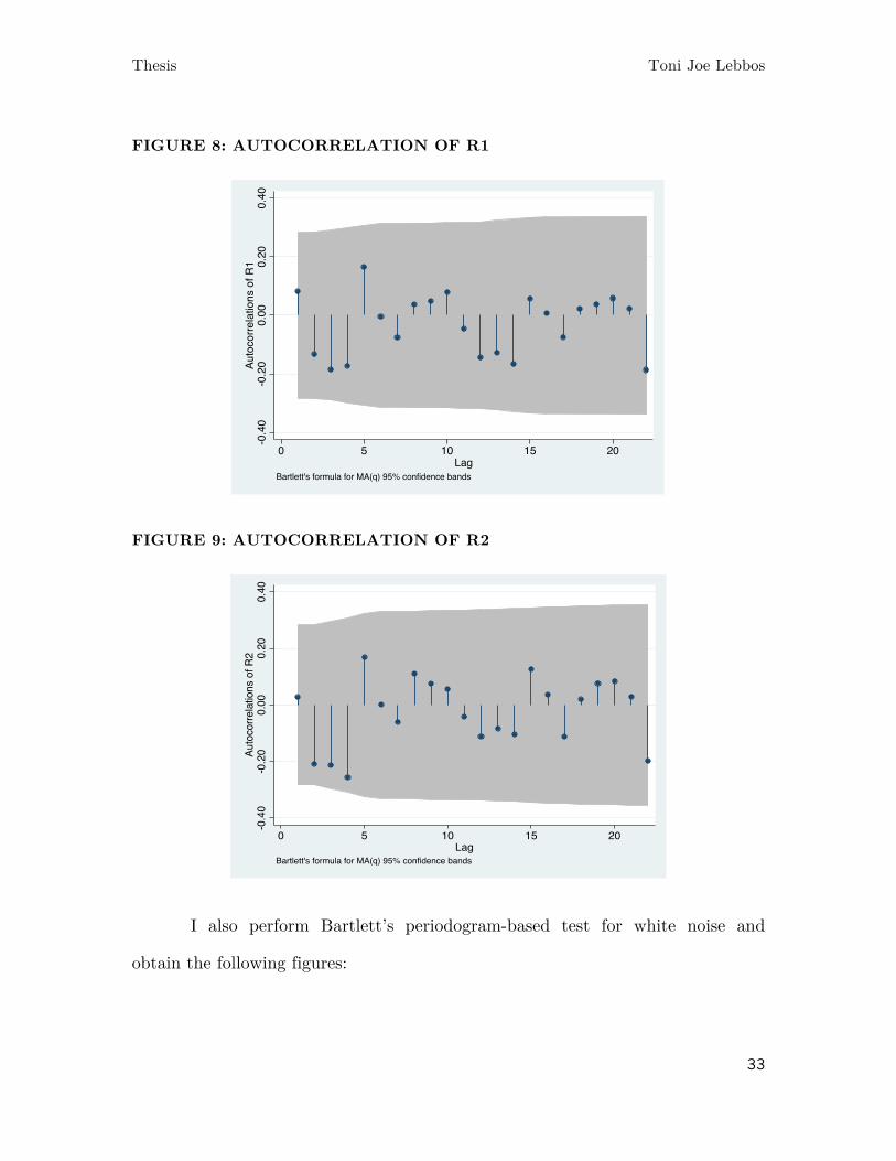
Testing further for autocorrelation and partial autocorrelation, I use
Stata’s corrgram command and find no significant autocorrelation in both
models:
-.05
0.05
.1.15
Residuals
1970 1980 1990 2000 2010 2020Year
Thesis Toni Joe Lebbos
33
FIGURE 8: AUTOCORRELATION OF R1
FIGURE 9: AUTOCORRELATION OF R2
I also perform Bartlett’s periodogram-based test for white noise and
obtain the following figures:
-0.4
0-0
.20
0.00
0.20
0.40
Auto
corre
latio
ns o
f R1
0 5 10 15 20Lag
Bartlett's formula for MA(q) 95% confidence bands
-0.4
0-0
.20
0.00
0.20
0.40
Auto
corre
latio
ns o
f R2
0 5 10 15 20Lag
Bartlett's formula for MA(q) 95% confidence bands

Thesis Toni Joe Lebbos
34
FIGURE 10: CUMULATIVE PERIODOGRAM WHITE-NOISE TEST R1
FIGURE 11CUMULATIVE PERIODOGRAM WHITE-NOISE TEST R2
Both figures indicate that we cannot reject the null hypothesis stating
there is no autocorrelation. This means that the residuals in both models are
0.00
0.20
0.40
0.60
0.80
1.00
Cum
ulat
ive
perio
dogr
am fo
r R1
0.00 0.10 0.20 0.30 0.40 0.50Frequency
Bartlett's (B) statistic = 0.71 Prob > B = 0.7011
Cumulative Periodogram White-Noise Test
0.00
0.20
0.40
0.60
0.80
1.00
Cum
ulat
ive
perio
dogr
am fo
r R2
0.00 0.10 0.20 0.30 0.40 0.50Frequency
Bartlett's (B) statistic = 0.59 Prob > B = 0.8761
Cumulative Periodogram White-Noise Test

Thesis Toni Joe Lebbos
35
random and that autocorrelation is not present. This is confirmed when running
a Portmanteau (Q) test for white noise that yield the following statistics and
further proves the absence of autocorrelation.
6.3 TESTING FOR MULTICOLLINEARITY
I test for multicollinearity using Variance Inflation Factors (vif). Those
latters test the magnitude to which the variance of estimated coefficients is
inflated because of multicollinearity. Results for both models show that GDP per
capita might be biasing estimates.
Consequently, I run both regressions again while omitting GDPpc and
obtain the following results:
TABLE 8: MODEL 1 ADJUSTED FOR MULTICOLLINEARITY
(1) VARIABLES annualized_standard_deviation_re
dvdexecutive 0.0390**
(0.0170) dvdlegislature 0.0511***
(0.0151) legelect 0.0341*
(0.0180) dummy_pre1987 -0.149***
(0.0360) inflation 0.0105***
(0.00342) cohesiveness 0.00228

Thesis Toni Joe Lebbos
36
(0.00220) distance 0.00243***
(0.000537) sociomood 0.000837
(0.00156) culturemood 0.00583***
(0.00174) Constant -0.312***
(0.0917)
Observations 49 R-squared
Adjusted R-Squared Root MSE F (9, 39) Prob > F
0.620 0.53237098
.04261 12.88 0.0000
Robust standard errors in parentheses *** p<0.01, ** p<0.05, * p<0.1
Notes: Dependent variable is volatility measured as the 20-days moving standard deviation of CAC 40/financial market indicator returns (unconditional volatility). Estimates are OLS estimates with robust standard errors. Dvdexecutive is a dummy variable that takes the value 1 if the executive branch of the government is divided, 0 otherwise. Dvdlegislature is a dummy variable that takes the value 1 if the legislative branch of the government is divided, 0 otherwise. Lgelect is a lag dummy variable accounting for years characterized by elections. Dummy_pre1987 is a dummy variable controlling for years before 1987 in which we use the financial market indicator instead of the CAC 40 in our computation of volatility. Inflation controls for fluctuations in consumer price index values. Cohesiveness is a measure of the ideological distance within the majority. Distance refers to the ideological distance between the majority and the opposition. Sociomood and Culturemood control for endogenous, global activation states with no specific external referent that might have an effect on volatility.
TABLE 9: MODEL 2 ADJUSTED FOR MULTICOLLINEARITY
(1) VARIABLES annualized_standard_deviation_re
0b.dvdexecutive#0b.dvdlegislature 0
(0) 0b.dvdexecutive#1.dvdlegislature 0.0313
(0.0203) 1.dvdexecutive#0b.dvdlegislature 0.0274
(0.0202) 1.dvdexecutive#1.dvdlegislature 0.101***
(0.0195) legelect 0.0335*

Thesis Toni Joe Lebbos
37
(0.0174) dummy_pre1987 -0.140***
(0.0349) inflation 0.00970***
(0.00347) cohesiveness 0.000699
(0.00252) distance 0.00231***
(0.000522) sociomood 0.000479
(0.00158) culturemood 0.00513***
(0.00178) Constant -0.237**
(0.101)
Observations 49 R-squared
Adjusted R-Squared Root MSE F(10, 38) Prob > F
0.636 0.54084013
.04222 17.48 0.0000
Robust standard errors in parentheses
*** p<0.01, ** p<0.05, * p<0.1 Notes: Dependent variable is volatility measured as the 20-days moving standard deviation of CAC 40/financial market indicator returns (unconditional volatility). Estimates are OLS estimates with robust standard errors. Dvdexecutive is a dummy variable that takes the value 1 if the executive branch of the government is divided, 0 otherwise. Dvdlegislature is a dummy variable that takes the value 1 if the legislative branch of the government is divided, 0 otherwise. 1.dvdexecutive#1.dvdlegislatur refers to situations in which both the legislative and the executive branches of the government are divided. Lgelect is a lag dummy variable accounting for years characterized by elections. Dummy_pre1987 is a dummy variable controlling for years before 1987 in which we use the financial market indicator instead of the CAC 40 in our computation of volatility. Inflation controls for fluctuations in consumer price index values. Cohesiveness is a measure of the ideological distance within the majority. Distance refers to the ideological distance between the majority and the opposition. Sociomood and Culturemood control for endogenous, global activation states with no specific external referent that might have an effect on volatility.
Both modified models have relatively similar results to their corresponding
previous initial models and estimates related to the main explanatory variables
are actually more statistically significant. In the adjusted model, having a divided
legislative branch seems to contribute to a 4.75% increase in stock market

Thesis Toni Joe Lebbos
38
volatility and having a divided executive branch seems to contribute to a 3.69%
increase in volatility. If both legislative and executive branches were divided,
model 2 suggests this would lead to a 9.56% increase in volatility.
6.4 EXCLUDING ABNORMAL OBSERVATION FROM SAMPLE
I rerun both initial models while excluding observations with abnormal
volatility values that coincide with times of financial crisis. The observations
removed are that of 2002 corresponding to the crash of the dot.com bubble and
that of 2008 corresponding to the global financial crises.
TABLE 10: MODEL 1 ADJUSTED FOR ABNORMAL ABSERVATIONS
(1) VARIABLES annualized_standard_deviation_re dvdexecutive 0.0435** (0.0174) dvdlegislature 0.0510*** (0.0158) dummy_pre1987 -0.149*** (0.0306) legelect 0.0131 (0.0136) inflation 0.00886*** (0.00261) gdppc -5.30e-06** (2.54e-06) cohesiveness 0.00170 (0.00226) distance 0.00129** (0.000626) sociomood 0.00164 (0.00137) culturemood 0.00694*** (0.00210) Constant -0.214* (0.113)

Thesis Toni Joe Lebbos
39
Observations 46 R-squared Adjusted R-Squared Root MSE F( 10, 35) Prob > F
0.618 0. 50920054
.03665 8.57
0.0000 Robust standard errors in parentheses
*** p<0.01, ** p<0.05, * p<0.1 Notes: Dependent variable is volatility measured as the 20-days moving standard deviation of CAC 40/financial market indicator returns (unconditional volatility). Estimates are OLS estimates with robust standard errors. Dvdexecutive is a dummy variable that takes the value 1 if the executive branch of the government is divided, 0 otherwise. Dvdlegislature is a dummy variable that takes the value 1 if the legislative branch of the government is divided, 0 otherwise. Lgelect is a lag dummy variable accounting for years characterized by elections. Dummy_pre1987 is a dummy variable controlling for years before 1987 in which we use the financial market indicator instead of the CAC 40 in our computation of volatility. Inflation controls for fluctuations in consumer price index values and GDPpc controls for fluctuation in GDP per capita. Cohesiveness is a measure of the ideological distance within the majority. Distance refers to the ideological distance between the majority and the opposition. Sociomood and Culturemood control for endogenous, global activation states with no specific external referent that might have an effect on volatility.
TABLE 11: MODEL 2 ADJUSTED FOR ABNORMAL OBSERVATIONS
(1) VARIABLES annualized_standard_deviation_re 0b.dvdexecutive#0b.dvdlegislature 0 (0) 0b.dvdexecutive#1.dvdlegislature 0.0291 (0.0211) 1.dvdexecutive#0b.dvdlegislature 0.0363* (0.0182) 1.dvdexecutive#1.dvdlegislature 0.107*** (0.0216) dummy_pre1987 -0.144*** (0.0304) legelect 0.0135 (0.0129) inflation 0.00845*** (0.00271) gdppc -5.65e-06** (2.46e-06) cohesiveness -0.000283 (0.00273) distance 0.00122*

Thesis Toni Joe Lebbos
40
(0.000637) sociomood 0.00106 (0.00138) culturemood 0.00647*** (0.00216) Constant -0.131 (0.116) Observations 46 R-squared Adjusted R-Squared Root MSE F(11, 34) Prob > F
0.637 0.52002274
.03624 10.03 0.0000
Robust standard errors in parentheses *** p<0.01, ** p<0.05, * p<0.1
Notes: Dependent variable is volatility measured as the 20-days moving standard deviation of CAC 40/financial market indicator returns (unconditional volatility). Estimates are OLS estimates with robust standard errors. Dvdexecutive is a dummy variable that takes the value 1 if the executive branch of the government is divided, 0 otherwise. Dvdlegislature is a dummy variable that takes the value 1 if the legislative branch of the government is divided, 0 otherwise. 1.dvdexecutive#1.dvdlegislatur refers to situations in which both the legislative and the executive branches of the government are divided. Lgelect is a lag dummy variable accounting for years characterized by elections. Dummy_pre1987 is a dummy variable controlling for years before 1987 in which we use the financial market indicator instead of the CAC 40 in our computation of volatility. Inflation controls for fluctuations in consumer price index values and GDPpc controls for fluctuation in GDP per capita. Cohesiveness is a measure of the ideological distance within the majority. Distance refers to the ideological distance between the majority and the opposition. Sociomood and Culturemood control for endogenous, global activation states with no specific external referent that might have an effect on volatility.
By excluding two abnormal observations from both models, results
obtained remain significant in the same direction in that states of divided
government lead to an increase in stock market volatility.
ACCOUNTING FOR CRISIS YEARS USING DUMMY VARIABLES To further assess the impact of crisis years on our estimation process, I
run both main models again while adding a dummy variable (crisis) to account
for years characterized by abnormal volatility values due to events such as a
financial market crisis.

Thesis Toni Joe Lebbos
41
Results for Model 1 are consistent with the previous analysis in that a
divided legislative branch and a divided executive branch are seen to separately
have a positive and statistically significant impact on stock market volatility.
Having a divided legislative branch increases stock market volatility by an
average of 4.06% and having a divided legislative branch increases volatility by
an average of 3.43%. Below is the output of the regression mentioned:
TABLE 12: MODEL 1 WITH ACCOUNTING FOR CRISIS YEARS
(1) VARIABLES annualized_standard_deviation_re
dvdexecutive 0.0343*
(0.0171) dvdlegislature 0.0406**
(0.0163) crisis 0.112***
(0.0342) dummy_pre1987 -0.144***
(0.0341) legelect 0.0170
(0.0134) inflation 0.00837***
(0.00271) gdppc -5.41e-06*
(2.70e-06) cohesiveness 0.00166
(0.00244) distance 0.000864
(0.000648) sociomood 0.00114
(0.00139) culturemood 0.00636***
(0.00213) Constant -0.133
(0.104)
Observations 48 R-squared 0.722

Thesis Toni Joe Lebbos
42
Adjusted R-Squared Root MSE
F( 11, 36) Prob > F
0. 63686846 .03772 10.35 0.0000
Robust standard errors in parentheses *** p<0.01, ** p<0.05, * p<0.1
Notes: Dependent variable is volatility measured as the 20-days moving standard deviation of CAC 40/financial market indicator returns (unconditional volatility). Estimates are OLS estimates with robust standard errors. Dvdexecutive is a dummy variable that takes the value 1 if the executive branch of the government is divided, 0 otherwise. Dvdlegislature is a dummy variable that takes the value 1 if the legislative branch of the government is divided, 0 otherwise. Crisis is a dummy variable that takes on the values 1 in years characterized by a financial crisis. Lgelect is a lag dummy variable accounting for years characterized by elections. Dummy_pre1987 is a dummy variable controlling for years before 1987 in which we use the financial market indicator instead of the CAC 40 in our computation of volatility. Inflation controls for fluctuations in consumer price index values and GDPpc controls for fluctuation in GDP per capita. Cohesiveness is a measure of the ideological distance within the majority. Distance refers to the ideological distance between the majority and the opposition. Sociomood and Culturemood control for endogenous, global activation states with no specific external referent that might have an effect on volatility.
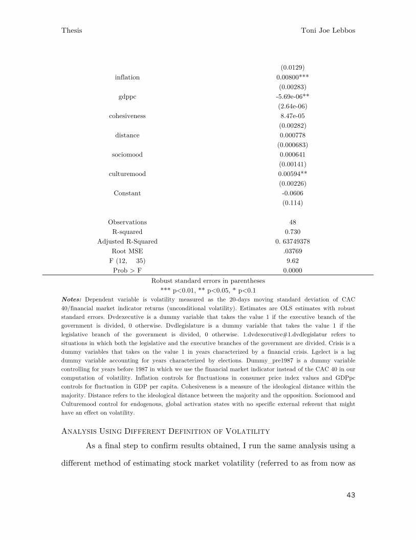
The second model is consistent as well with previous results. Even when
accounting for crisis years. It indicates that having a divided legislative branch
and a divided executive branch simultaneously contributes to an increase in stock
market volatility by 8.31%.
TABLE 13: MODEL 2 WITH ACCOUNTING FOR CRISIS
(1) VARIABLES annualized_standard_deviation_re
0b.dvdexecutive#0b.dvdlegislature 0
(0) 0b.dvdexecutive#1.dvdlegislature 0.0223
(0.0217) 1.dvdexecutive#0b.dvdlegislature 0.0278
(0.0186) 1.dvdexecutive#1.dvdlegislature 0.0831***
(0.0215) crisis 0.106***
(0.0372) dummy_pre1987 -0.140***
(0.0340) legelect 0.0177
Thesis Toni Joe Lebbos
43
(0.0129) inflation 0.00800***
(0.00283) gdppc -5.69e-06**
(2.64e-06) cohesiveness 8.47e-05
(0.00282) distance 0.000778
(0.000683) sociomood 0.000641
(0.00141) culturemood 0.00594**
(0.00226) Constant -0.0606
(0.114)
Observations 48 R-squared
Adjusted R-Squared Root MSE
F (12, 35) Prob > F
0.730 0. 63749378
.03769 9.62
0.0000 Robust standard errors in parentheses
*** p<0.01, ** p<0.05, * p<0.1 Notes: Dependent variable is volatility measured as the 20-days moving standard deviation of CAC 40/financial market indicator returns (unconditional volatility). Estimates are OLS estimates with robust standard errors. Dvdexecutive is a dummy variable that takes the value 1 if the executive branch of the government is divided, 0 otherwise. Dvdlegislature is a dummy variable that takes the value 1 if the legislative branch of the government is divided, 0 otherwise. 1.dvdexecutive#1.dvdlegislatur refers to situations in which both the legislative and the executive branches of the government are divided. Crisis is a dummy variables that takes on the value 1 in years characterized by a financial crisis. Lgelect is a lag dummy variable accounting for years characterized by elections. Dummy_pre1987 is a dummy variable controlling for years before 1987 in which we use the financial market indicator instead of the CAC 40 in our computation of volatility. Inflation controls for fluctuations in consumer price index values and GDPpc controls for fluctuation in GDP per capita. Cohesiveness is a measure of the ideological distance within the majority. Distance refers to the ideological distance between the majority and the opposition. Sociomood and Culturemood control for endogenous, global activation states with no specific external referent that might have an effect on volatility.
ANALYSIS USING DIFFERENT DEFINITION OF VOLATILITY As a final step to confirm results obtained, I run the same analysis using a
different method of estimating stock market volatility (referred to as from now as

Thesis Toni Joe Lebbos
44
Method 2). In this method, I compute stock market volatility by simply taking
the standard deviation of returns throughout each year.
Results are consistent with our previous findings in that divided
government is seen to have a positive and statistically significant impact on stock
market volatility. Model 1 indicates that, empirically, having a divided legislative
branch of the government contributes to an increase in volatility by 1.12%. The
table below represents the output of the regression mentioned:
TABLE 14: MODEL 1 USING METHOD 2
(1) VARIABLES Volatility dvdexecutive 0.00131 (0.00311) dvdlegislature 0.0112** (0.00461) legelect 0.00865* (0.00469) pre1987 -0.0160 (0.0132) inflation 0.00312** (0.00119) gdppc -1.35e-06 (1.22e-06) cohesiveness 0.00153* (0.000825) distance 0.000307 (0.000227) sociomood 0.000503 (0.000468) culturemood 0.00107 (0.000726) Constant -0.0558* (0.0279) Observations 48 R-squared 0.680

Thesis Toni Joe Lebbos
45
Adjusted R-Squared Root-MSE F (10, 37) Prob > F
0. 59393498 .01045 11.52 0.0000
Robust standard errors in parentheses *** p<0.01, ** p<0.05, * p<0.1
Notes: Dependent variable is volatility measured as the standard deviation of CAC 40/financial market indicator returns. Estimates are OLS estimates with robust standard errors. Dvdexecutive is a dummy variable that takes the value 1 if the executive branch of the government is divided, 0 otherwise. Dvdlegislature is a dummy variable that takes the value 1 if the legislative branch of the government is divided, 0 otherwise. Lgelect is a lag dummy variable accounting for years characterized by elections. Dummy_pre1987 is a dummy variable controlling for years before 1987 in which we use the financial market indicator instead of the CAC 40 in our computation of volatility. Inflation controls for fluctuations in consumer price index values and GDPpc controls for fluctuation in GDP per capita. Cohesiveness is a measure of the ideological distance within the majority. Distance refers to the ideological distance between the majority and the opposition. Sociomood and Culturemood control for endogenous, global activation states with no specific external referent that might have an effect on volatility.
Model 2 indicates that having simultaneously a divided executive branch
and a divided legislative branch contributes to an increase in volatility by around
1.04%. The table below represents the output of the regression:
TABLE 15: MODEL 2 USING METHOD 2
VARIABLES Volatility
0b.dvdexecutive#0b.dvdlegislature 0 (0)
0b.dvdexecutive#1.dvdlegislature 0.0163 (0.0102)
1.dvdexecutive#0b.dvdlegislature 0.00319 (0.00408)
1.dvdexecutive#1.dvdlegislature 0.0104*** (0.00270)
legelect 0.00856* (0.00461)
pre1987 -0.0158 (0.0128)
inflation 0.00316** (0.00120)
gdppc -1.17e-06 (1.21e-06)
cohesiveness 0.00195

Thesis Toni Joe Lebbos
46
(0.00122) distance 0.000338
(0.000239) sociomood 0.000651
(0.000527) culturemood 0.00115
(0.000784) Constant -0.0781
(0.0476)
Observations 48 R-squared
Adjusted R-Squared Root-MSE F (11, 36) Prob > F
0.690 0.59519688
.01044 9.64
0.0000 Robust standard errors in parentheses
*** p<0.01, ** p<0.05, * p<0.1 Notes: Dependent variable is volatility measured as the standard deviation of CAC 40/financial market indicator returns. Estimates are OLS estimates with robust standard errors. Dvdexecutive is a dummy variable that takes the value 1 if the executive branch of the government is divided, 0 otherwise. Dvdlegislature is a dummy variable that takes the value 1 if the legislative branch of the government is divided, 0 otherwise. 1.dvdexecutive#1.dvdlegislatur refers to situations in which both the legislative and the executive branches of the government are divided. Lgelect is a lag dummy variable accounting for years characterized by elections. Dummy_pre1987 is a dummy variable controlling for years before 1987 in which we use the financial market indicator instead of the CAC 40 in our computation of volatility. Inflation controls for fluctuations in consumer price index values and GDPpc controls for fluctuation in GDP per capita. Cohesiveness is a measure of the ideological distance within the majority. Distance refers to the ideological distance between the majority and the opposition. Sociomood and Culturemood control for endogenous, global activation states with no specific external referent that might have an effect on volatility.
Since results in our first estimation (Method 1) also indicate a positive
relationship between divided states of the government and stock market
volatility, outcomes from this robustness check are coherent and confirm our
previous analysis.
8 LIMITATIONS The analysis conducted could be improved in various manners. A first step
for improvement would be to increase sample size either by considering a larger

Thesis Toni Joe Lebbos
47
time span or by dissecting further the yearly data provided (gathering quarterly
data instead of yearly for instance). Also, different ways of defining divided vs.
unified could be tested out to examine further the impact of different parts of the
government of stock market volatility. Another suggestion would be to add more
countries to the analysis; this however raises the question of whether results are
truly comparable given the different political systems used. Another limitation is
the use of two different indicators as a proxy for the performance of the French
stock market. A smoother analysis is expected for countries that have used the
same performance indicator for the entirety of the analysis.
9 CONCLUSION In conclusion, this paper tackles an interesting conundrum that has yet to
see more empirical proof throughout the world. The literature review conducted
provides a rigorous base of intuition and insight regarding the existing literature.
Two main conflicting notions are tackled: the notion of a gridlock effect that is
expected to decrease stock market volatility by assuaging policy risk and the
notion that government structure and patterns of control have no significant
impact on stock market volatility. Findings of this study reject the gridlock
hypothesis and argue that having a divided government (divided legislative and
divided executive branches) contributes to an increase in stock market volatility.
This fits well with Conley (2007)’s claim that major shifts in the political
landscape have happened in periods of divided government and giving intuitive
sense to the rise in stock market volatility during those periods. These finding
carry implications for further research in political economics and financial
markets. Also, an increase in stock market volatility often leads to the

Thesis Toni Joe Lebbos
48
deterioration of capital investment by risk-averse investors. Considering such
effects, an important implication of our result is states of divided governments
might be a key explanatory variable in determining inflow levels of capital stock.
Further research could, in addition to expanding sample size, look more into the
different companies composing the CAC 40 companies and their political
proximity to the government. Assessing the variation of their stock prices given
different states of the government could yield interesting results.

Thesis Toni Joe Lebbos
49
BIBLIOGRAPHY Alenisa, A., & Rosenthal, H. (1995). Partisan Politics, Divided Government, and the Economy. Cambridge: Cambridge University Press.
Baumgartner, F. R., Brouard, S., Grossman, E., Lazardeux, S., & Moody, J. (2014). Divided Government, Legislative Productivity, and Policy Change in the USA and France. Governance: An International Journal of Policy, Administration, and Institutions , 27 (3), 423–447.
Bechtel, M., & Fuss, R. (2008). When Investors Enjoy Less Policy Risk: Divided Government, Economic Policy Change, and Stock Market Volatility, 1970-2005. Swiss Political Science Review , 14 (2), 287-314.
Conley, R. S. (2007). Presidential Republics and Divided Government: Law-Making and Executive Politics in the United States and France. Political science Quarterly , 122 (2), 257–285.
Datastream. (2016). Thomson Reuters Datastream. Retrieved March 2016, from Financial Data.
Euronext. (2016). Euronext. Retrieved 01 04, 2016, from Euronext: https://www.euronext.com/en
Fiorina, M. (1992). Divided Government. New York: Macmillan Publishing Company.
Fowler, J. H. (2006). Elections and Markets: The Effect of Partisanship, Policy Risk, and Electoral Margins on the Economy. The Journal of Politics , 68 (1), pp. 89–103.
Francais, G. (2016). Gouvernement . Retrieved 01 02, 2016, from Gouvernement.fr: http://www.gouvernement.fr/en/composition-of-the-government
Francais, G. (2015). Gouvernement.fr. Retrieved 11 05, 2015, from Gouvernement.fr: http://www.gouvernement.fr
Howell, W., Adler, S., Cameron, C., & Riemann, C. (2000). Divided Government and the Legislative Productivity of Congress, 1945–94. Legislative Studies Quarterly , 25 (2), 285–312.

Thesis Toni Joe Lebbos
50
Karol, D. (2000). Divided Government and U.S. Trade Policy: Much Ado About Nothing? International Organization , 54 (4), 825–44 .
Kim, C., Pantzalis, C., & Park, C. C. (2012). Political Geography and Stock Returns: The Value and Risk Implications of Proximity to Political Power . Journal of Financial Economics , 106, 196-228.
Kobrin, S. J. (1982). Managing Political Risk Assessment: Strategic Response to Environmental Change. California: University of California Press.
Krehbiel, K. (1998). Pivotal Politics: A Theory of U.S. Lawmaking. Chicago: University of Chicago Press.
Lazardeux, S. (2009). Cohabitation and Policymaking Efficiency in Semi- Presidential Systems. Seattle, WA: Department of Political Science, University of Washington.
Lohmann, S., & O’Halloran, S. (1994). Divided Government and U.S. Trade Policy: Theory and Evidence. International Organization , 48 (4), 595–632.
Mayhew, D. R. (1991). Divided We Govern: Party Control, Lawmaking, and Investigations 1946–1990. New Haven, CT: Yale University Press.
Milner, H., & Rosendorff, P. (1996). Democratic Politics and International Trade Negotiations: Elections and Divided Government as Constraints on Trade Liberalization. Journal of Conflict Resolution , 41 (1), 117–46.
Pantzalis, C., Stangeland, D., & Turtle, H. (2000). Political Elections and the Resolution of Uncertainty. Journal of Banking and Finance , 24 (10), 1575–604.
Parker, W. D. (2007). The Socionomic Perspective on Social Mood and Voting: Report on New Mood Measures in the 2006 ANES Pilot Study. ANES Pilot Study Report.
Poterba, J. (1994). State Responses to Fiscal Crisis: The Effects of Budgetary Institutions and Policies. Journal of Political Economy , 102 (4), 799–821.
Prechter, J., & Robert, R. (n.d.). The Wave Principle of Human Social Behavior and the New Science of Socionomics. Gainesville, GA: New Classics Library. , 1999.

Thesis Toni Joe Lebbos
51
Prechter, J., Goel, D., & Parker, W. (2007). We know how you’ll vote next November: social mood, financial markets and presidential election outcomes. Working paper, Socionomics Foundation, Gainesville, Georgia.
Roubini, N., & J, S. (1989). Political and Economic Determinants of Budget Deficits in the Industrial Democracies. European Economic Review , 33 (5), 903–38 .
Siaroff, A. (2003). Comparative Presidencies: The Inadequacy of the Presidential, Semi-Presidential and Parliamentary Distinction. European Journal of Political Research , 42 (3), 287–312.
Tsebelis, G. (1995). eto Players and Law Production in Parliamentary Democracies n Parliaments and Majority Rule in Western Europe (Vol. V). (H. Döring, Ed.) New York: St. Martin’s Press.
Wikipedia. (2016). Politics of France. Retrieved 01 29, 2016, from Wikipedia: https://en.wikipedia.org/wiki/Politics_of_France
World Bank. (2016). World Development Indicators. Retrieved March 2016, from The World Bank: http://databank.worldbank.org/data/reports.aspx?source=world-development-indicators
Wright, I., Sloman, A., & Beaudoin, L. (1996). Towards a design based analysis of emotional episodes. Philosophy, Psychiatry and Psychology , 3 (2), 101-137.

Thesis Toni Joe Lebbos
52
ANNEXES
ANNEX 1: MODEL 1 & 2 OUTPUT EXCLUDING MAIN EXPLANATORY VARIABLES

Thesis Toni Joe Lebbos
53
ANNEX 2: MODEL 1 OUTPUT
ANNEX 3: MODEL 2 OUTPUT

Thesis Toni Joe Lebbos
54
ANNEX 3: STANDARD DURBIN WATSON D-STATISTIC MODEL 1 & 2
ANNEX 4: CORRGRAM OUTPUT MODEL 1 & 2

Thesis Toni Joe Lebbos
55
ANNEX 5: MULTICOLLINEARITY TEST
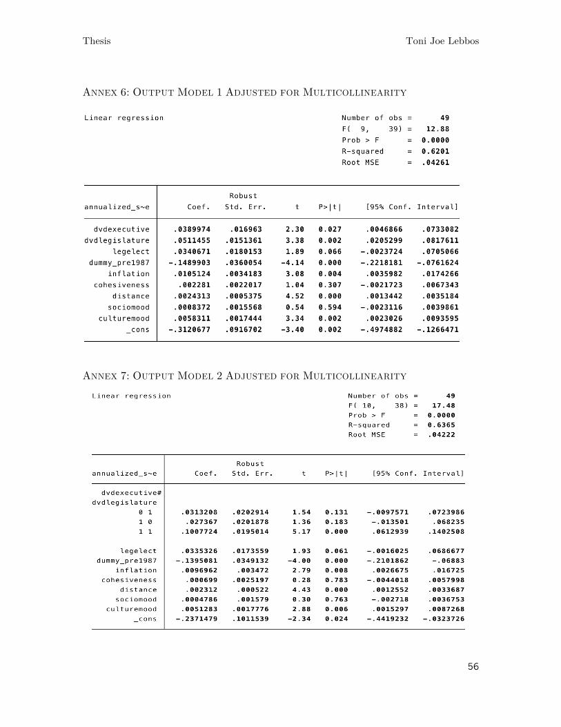
Thesis Toni Joe Lebbos
56
ANNEX 6: OUTPUT MODEL 1 ADJUSTED FOR MULTICOLLINEARITY
ANNEX 7: OUTPUT MODEL 2 ADJUSTED FOR MULTICOLLINEARITY
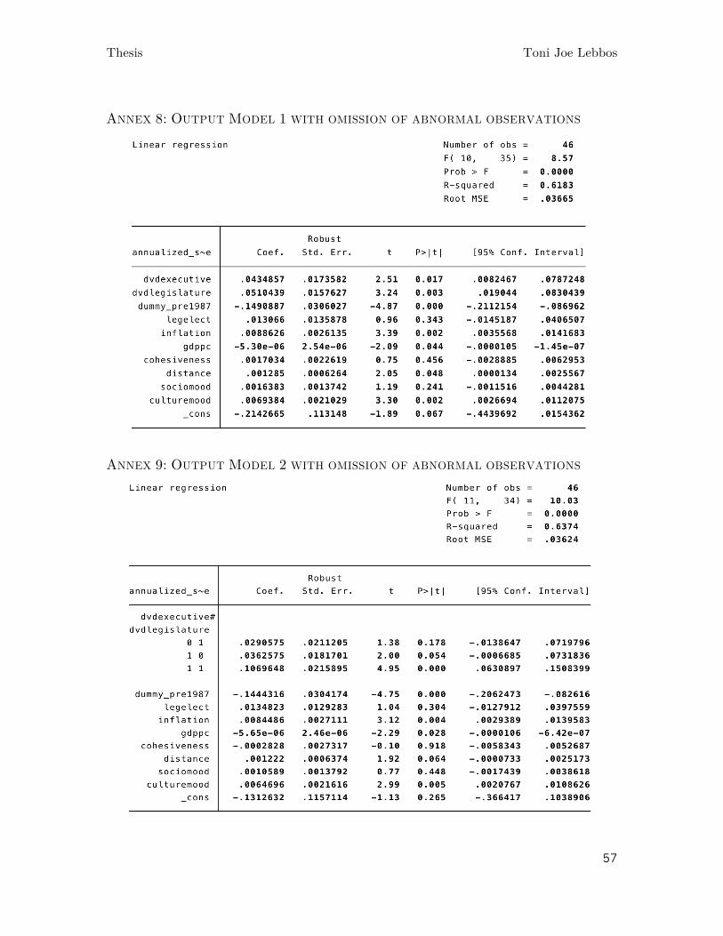
Thesis Toni Joe Lebbos
57
ANNEX 8: OUTPUT MODEL 1 WITH OMISSION OF ABNORMAL OBSERVATIONS
ANNEX 9: OUTPUT MODEL 2 WITH OMISSION OF ABNORMAL OBSERVATIONS

Thesis Toni Joe Lebbos
58
ANNEX 10: OUTPUT MODEL 1 WITH ACCOUNTING FOR CRISIS YEARS
ANNEX 11: OUTPUT MODEL 2 WITH ACCOUNTING FOR CRISIS YEARS

Thesis Toni Joe Lebbos
59
ANNEX 12: OUTPUT MODEL 1 USING METHOD 2
ANNEX 13: OUTPUT MODEL 2 USING METHOD 2

Thesis Toni Joe Lebbos
60
ANNEX 14: MODELS 1 & 2 WITH INTEREST INCLUDED AS EXPLANATORY
VARIABLE