financial optimization problems in life and pension … · financial optimization problems in life...
TRANSCRIPT

Financial Optimization Problems
in Life and Pension Insurance
Peter Holm Nielsen
Thesis submitted for the Ph.D. degree
Laboratory of Actuarial Mathematics
Department of Applied Mathematics and Statistics
Institute for Mathematical Sciences
Faculty of Science
University of Copenhagen
Supervisors:
Hanspeter Schmidli
Mogens Steffensen
Thesis committee:
Martin Jacobsen, University of Copenhagen
Ralf Korn, University of Kaiserslautern
Fred Espen Benth, University of Oslo
December 2005

Preface
This thesis has been prepared in partial fulfillment of the requirements for thePh.D. degree at the Laboratory of Actuarial Mathematics in the Department ofApplied Mathematics and Statistics, Institute for Mathematical Sciences, Facultyof Science, University of Copenhagen. The work has been carried out in the periodfrom December 2002 to December 2005 under the supervision of Hanspeter Schmidli(University of Copenhagen until November 2004; now University of Cologne) andMogens Steffensen (University of Copenhagen).
Acknowledgements
I would like to thank Hanspeter Schmidli for encouragement and support, andfor comments on early versions of the published papers. I am deeply indebted toMogens Steffensen for his encouragement, support, and general guidance, and formany valuable discussions in relation to my work as well as to other matters. Hehas played a role of great significance as a supervisor, colleague, and friend.
I also wish to thank Ragnar Norberg, former professor at the Laboratory ofActuarial Mathematics at the University of Copenhagen and supervisor of my Mas-ter’s Thesis, who encouraged me to take the plunge and study for the Ph.D. degree.His continued interest, support, encouragement, and willingness to share and dis-cuss ideas have been remarkable. He also made the necessary arrangements toensure that a desk was provided for me at the Financial Markets Group at theLondon School of Economics during my stay in London from September 2003 toJanuary 2004.
I highly appreciate the support and interest shown to me by many of my col-leagues, academics as well as practitioners. I wish to mention in particular MikkelDahl, my fellow Ph.D. student and close colleague at the Laboratory of ActuarialMathematics, with whom I have had a host of fruitful discussions. I also wish tothank Martin Jacobsen for his kindness and willingness to answer technical ques-tions, Thomas Møller for his encouragement and guidance in the field of quadratichedging approaches, and Jørgen Steen Larsen for his kindness and willingness toshare his extensive knowledge about and insight in the insurance practice.
Furthermore, I want to thank my family and friends for general support, en-couragement, understanding, and patience during the past three years. Special
i

thoughts go to my girlfriend, Signe, and our little son, Josias.Finally, I wish to thank for financial support from the Danish Society of Actuar-
ies for my participation in “The Nordic Summer School in Insurance Mathematics2003”, and from Knud Højgaards Fond and Christian og Ottilia Brorsons Rejselegatfor my stay in London.
ii

Summary
This thesis deals with certain financial optimization problems connected to lifeand pension insurance. We take the perspective of a life insurance company ora pension fund that aims to optimize certain strategies related to the design andmanagement of life and pension insurance policies, in particular investment andbonus strategies, on behalf of the policyholders and/or on behalf of the companyitself (i.e., its owners).
Traditional life insurance mathematics is an actuarial discipline mainly con-cerned with qualitative and quantitative analyses of various aspects of risks con-nected to life and pension insurance policies, in particular modelling and assessmentof mortality, calculation of present values and (equivalence) premiums, etc. Thetools and principles for management of (portfolios of) life and pension insurancepolicies are to some extent also subjects of this field, but they are traditionallyderived only implicitly from the abovementioned analyses or on the basis of moreor less ad hoc considerations, that is, specific optimization criteria are rarely con-sidered.
In this thesis we formulate and treat explicit optimization problems that formal-ize certain objectives of a life or pension insurance company arising from the naturaldesire to optimize the management, in a broad sense, of the portfolio of policiesand the company as a whole. We apply and extend methods from mathematicalfinance, which is a mathematical/economical discipline concerned with various as-pects of financial markets, in particular optimization of investment strategies indifferent respects.
The first main chapter of the thesis, Chapter 2, presents a survey of the lit-erature on optimal investment theory. We attempt to cover most of the classicalproblems and approaches; we begin with the single-period analyses dating back tothe beginning of the 1950’s and plough our way through the literature chronolog-ically. The amount of research conducted in this field has increased dramaticallyover the past 10-15 years, and we only go through a fraction of the modern litera-ture. The theory of optimal investment obviously has substantial relevance in lifeand pension insurance (in particular pension saving), but we point out that theapplication of this theory in life and pension insurance by no means is trivial ingeneral.
Chapters 3 and 4 deal with optimization problems concerning, in a broad sense,optimal redistribution of the systematic surplus generated by a generic so-called
iii

participating life insurance policy, although other interpretations are possible inthe model of Chapter 4. The problems are in some sense similar in nature, butthe chapters represent quite different approaches. In Chapter 3 we work within atraditional setup of life insurance mathematics; in particular we do not considerdifferent investment possibilities. In Chapter 4 we consider a fairly general modelthat explicitly includes a financial market model, and we propose an overall generalapproach to the optimal management of life and pension insurance policies. Inboth chapters we take the policy risks explicitly into account, but we treat themdifferently.
The last chapter addresses an important problem that arises in connection withthe application of methods of mathematical finance for optimal investment in lifeand pension insurance. Life and pension insurance policies are often very long-termcontracts, and from a practical point of view it is therefore quite unrealistic to as-sume the financial market to be complete over the full term of the policies sincereal-world markets in particular typically only offer bonds (and other interest ratederivatives) of a limited duration. The problem of optimal investment in life andpension insurance is further complicated by the fact that long-term minimum guar-antees, for which the natural hedging derivatives are bonds, often are included inthe policies. We consider a purely financial (i.e., no policy risk involved) optimiza-tion problem of a long-term investor in a fairly simple model of a financial marketthat exhibits the lack of long-term bonds (and other interest rate derivatives) inreal-world markets.
iv

Resume
Denne afhandling behandler visse finansielle optimeringsproblemer knyttet til livs-og pensionsforsikring. Vi tager udgangspunkt i perspektivet for et livsforsikrings-selskab eller en pensionskasse, der sigter mod at optimere visse strategier relaterettil designet og styringen af livs- og pensionsforsikringspolicer, specielt investerings-og bonusstrategier, pa vegne af policetagerne og/eller pa vegne af selskabet selv(dvs. dets ejere).
Traditionel livsforsikringsmatematik er en aktuarmæssig disciplin, der hoved-sageligt beskæftiger sig med kvalitative og kvantitative analyser af forskellige as-pekter af risici knyttet til livs- og pensionsforsikringspolicer, specielt modelleringog vurdering af dødelighed, beregning af nutidsværdier og (ækvivalens-)præmier,etc. Værktøjerne og principperne for styring af (porteføljer af) livs- og pensions-forsikringspolicer er til en vis grad ogsa emner inden for dette felt, men de udledestraditionelt kun implicit fra ovennævnte analyser eller pa basis af mere eller mindread hoc betragtninger, dvs. specificikke optimeringskriterier betragtes sjældent.
I denne afhandling formulerer og behandler vi eksplicitte optimeringsproblemerder formaliserer visse mal for et livsforsikringsselskab eller en pensionskasse, somopstar fra det naturlige ønske om at optimere styringen, i en bred forstand, afporteføljen af policer og selskabet som helhed. Vi anvender og udvider metoder framatematisk finansiering, som er en matematisk/økonomisk disciplin, der beskæfti-ger sig med forskellige aspekter af finansielle markeder, specielt optimering af in-vesteringsstrategier til forskellige formal.
Det første hovedkapitel i afhandlingen, Kapitel 2, præsenterer en oversigt overlitteraturen om optimal investeringsteori. Vi forsøger at dække de fleste klassiskeproblemer og tilgange; vi begynder med en-periode analyserne, der daterer sig tilbegyndelsen af 1950’erne, og pløjer os gennem litteraturen kronologisk. Mængdenaf forskning der udføres inden for dette felt er vokset dramatisk de sidste 10-15ar, og vi gennemgar kun en del af den moderne litteratur. Teorien om optimalinvestering har naturligvis betydelig relevans for livs- og pensionsforsikring (specieltfor pensionsopsparing), men vi gør opmærksom pa, at anvendelsen af denne teori ilivs- og pensionsforsikring pa ingen made er triviel generelt.
Kapitel 3 og 4 behandler optimeringsproblemer, der vedrører optimal tilbagefør-sel, i en bred forstand, af det systematiske overskud, der genereres af en livsfor-sikringspolice med bonusret, omend andre fortolkninger er mulige i modellen i Kapi-tel 4. Problemerne ligner i en vis forstand hinanden, men kapitlerne repræsenterer
v

ret forskellige tilgange. I Kapitel 3 arbejder vi inden for en traditionel opsæt-ning i livsforsikringsmatematik; specielt betragter vi ikke forskellige investerings-muligheder. I Kapitel 4 betragter vi en temmelig generel model, som eksplicitinkluderer en model af et finansielt marked, og vi foreslar en overordnet tilgangtil optimal styring af livs- og pensionsforsikringspolicer. I begge kapitler tager vipolicerisiciene eksplicit i betragtning, men vi behandler dem forskelligt.
Det sidste kapitel adresserer et vigtigt problem, der opstar i forbindelse med an-vendelsen af metoder fra matematisk finansieringsteori til optimal investering i livs-og pensionsforsikring. Livs- og pensionsforsikringspolicer er ofte meget langsigtedekontrakter, og fra et praktisk synspunkt er det derfor ret urealistisk at antage, at detfinansielle marked er fuldstændigt over policernes fulde løbetider, eftersom virke-lighedens markeder specielt kun udbyder obligationer (og andre rentederivater) afbegrænset varighed. Problemet om optimal investering i livs- og pensionsforsikringkompliceres yderligere af det forhold, at langsigtede minimumsgarantier, hvortil denaturlige afdækningsinstrumenter er obligationer, ofte er inkluderet i policerne. Vibetragter et rent finansielt (dvs. ingen policerisiko involveret) optimeringsproblemfor en langsigtet investor i en ret simpel model for et finansielt marked, som ud-stiller manglen pa lange obligationer (og andre rentederivater) pa virkelighedensmarkeder.
vi

Contents
Preface i
Summary iii
Resume v
1 Introduction 1
1.1 A brief comparison with related fields of research . . . . . . . . . . . 1
1.2 General scope and aims of the thesis . . . . . . . . . . . . . . . . . . 3
1.3 Overview and contributions of the thesis . . . . . . . . . . . . . . . . 5
2 A Survey on Investment Theory 7
2.1 Introduction . . . . . . . . . . . . . . . . . . . . . . . . . . . . . . . . 7
2.2 A general financial market model . . . . . . . . . . . . . . . . . . . . 8
2.3 Optimization objectives and solution techniques . . . . . . . . . . . . 18
2.4 Single-period portfolio selection . . . . . . . . . . . . . . . . . . . . . 21
2.5 Multi-period portfolio selection . . . . . . . . . . . . . . . . . . . . . 26
2.6 Continuous-time portfolio selection . . . . . . . . . . . . . . . . . . . 29
2.7 The martingale method . . . . . . . . . . . . . . . . . . . . . . . . . 41
2.8 Problems with stochastic interest rates . . . . . . . . . . . . . . . . . 49
2.9 Effects of inflation . . . . . . . . . . . . . . . . . . . . . . . . . . . . 56
2.10 Some concluding remarks . . . . . . . . . . . . . . . . . . . . . . . . 57
3 Optimal Bonus Strategies in Life Insurance: The Markov Chain
Interest Rate Case 59
3.1 Introduction . . . . . . . . . . . . . . . . . . . . . . . . . . . . . . . . 59
3.2 Basics . . . . . . . . . . . . . . . . . . . . . . . . . . . . . . . . . . . 62
3.3 Statement of the problem . . . . . . . . . . . . . . . . . . . . . . . . 65
3.4 Control theory . . . . . . . . . . . . . . . . . . . . . . . . . . . . . . 66
3.5 Discussions and conclusion . . . . . . . . . . . . . . . . . . . . . . . . 77
3.6 Generalizations . . . . . . . . . . . . . . . . . . . . . . . . . . . . . . 81
vii

4 Utility Maximization and Risk Minimization in Life and Pension
Insurance 89
4.1 Introduction . . . . . . . . . . . . . . . . . . . . . . . . . . . . . . . . 894.2 The model . . . . . . . . . . . . . . . . . . . . . . . . . . . . . . . . . 924.3 The optimization problem . . . . . . . . . . . . . . . . . . . . . . . . 974.4 General results on dividend optimization . . . . . . . . . . . . . . . . 1034.5 Quadratic hedging strategies . . . . . . . . . . . . . . . . . . . . . . 1094.6 A worked-out example . . . . . . . . . . . . . . . . . . . . . . . . . . 1144.7 Conclusions . . . . . . . . . . . . . . . . . . . . . . . . . . . . . . . . 1184.8 Discussions and generalizations . . . . . . . . . . . . . . . . . . . . . 1194.9 A comparison with Steffensen (2004) . . . . . . . . . . . . . . . . . . 124
5 On Optimal Long-term Investment in a Market Without Long-
term Bonds 137
5.1 Introduction . . . . . . . . . . . . . . . . . . . . . . . . . . . . . . . . 1375.2 The general market . . . . . . . . . . . . . . . . . . . . . . . . . . . . 1395.3 The optimization problem . . . . . . . . . . . . . . . . . . . . . . . . 1445.4 The complete-market case . . . . . . . . . . . . . . . . . . . . . . . . 1465.5 An extended Vasicek term structure . . . . . . . . . . . . . . . . . . 1485.6 An extended Cox-Ingersoll-Ross term structure . . . . . . . . . . . . 1535.7 Conclusion . . . . . . . . . . . . . . . . . . . . . . . . . . . . . . . . 164
A Some Utility Theory 165
A.1 The expected utility maxim: Basics . . . . . . . . . . . . . . . . . . . 165A.2 Definition and basic properties of utility functions . . . . . . . . . . 167A.3 HARA utility functions . . . . . . . . . . . . . . . . . . . . . . . . . 168A.4 The expected utility maxim: Discussion . . . . . . . . . . . . . . . . 169A.5 Proper risk aversion . . . . . . . . . . . . . . . . . . . . . . . . . . . 175
B Convex Analysis 177
B.1 Convex analysis . . . . . . . . . . . . . . . . . . . . . . . . . . . . . . 177B.2 Some remarks on intuition . . . . . . . . . . . . . . . . . . . . . . . . 179
C Elliptical Distributions 181
C.1 Definition and properties . . . . . . . . . . . . . . . . . . . . . . . . . 181
Bibliography 183
viii

Chapter 1
Introduction
This introductory chapter briefly relates the problems considered in this thesis torelevant fields of research in a fairly nontechnical manner. Furthermore, the natureand scope of the considered problems is clarified, without attention to details.Finally, an overview of the contents of the thesis is provided.
1.1 A brief comparison with related fields of research
The topics of this thesis lie at the interface between life insurance mathematicsand mathematical finance. These two fields of research have, until quite recently,evolved more or less independently of one another.
Classical topics of life insurance mathematics (see, e.g., Norberg (2000) or Ger-ber (1997)) are, in broad terms, modelling and estimation of policy risks (i.e.,mortality risk and other risks associated with the random course of life of the in-sured under a life or pension insurance policy), the study of particular forms ofpolicies, calculations and characterizations of reserves (and higher order momentsof present values), premium calculations, etc.
Explicit modelling of the financial market in which a policy is issued is typicallynot an issue that is addressed in basic life insurance mathematics, where only aspecific model of the policy risk is considered. As regards the financial aspects of lifeinsurance, the traditional overall approach (to so-called participating or with-profitlife insurance policies, at least) has been to simply base the calculation of premiumson a prudent (pessimistic) assessment of the future interest rates, the idea beingthat the actual yields from investments should be sufficient to cover the liabilitiesunder virtually any conceivable economic development over the policy terms, seee.g. Norberg (1999) (the traditional approach regarding the aspects related to thepolicy risks is fairly similar, but we do not go into details since we mainly focus onthe financial aspects). Thus, a formalization of investment strategies employed inrelation to the (portfolio of) policies has traditionally not been studied as a topicin basic life insurance mathematics.
This approach raises several natural questions: How should life and pension
1

2 Chapter 1
insurance companies invest in the financial market? More generally, how shouldthey manage their policies? How should the systematic surplus that typicallyemerges over the policy terms (due to the prudent assessment of future interestrates) be redistributed to the policyholder(s)? What criteria should be imposed toensure that policies are fair? What happens if the actual yields from investmentsare insufficient to cover the liabilities? Can this be avoided with certainty? A moregeneral and fundamental question along these lines is: How should life and pensioninsurance policies be designed, and how should they be managed? Let us interposethe remark that some of these questions are very much of current interest in thepractical world of life and pension insurance.
Classical topics of mathematical finance (see, e.g., Karatzas and Shreve (1998)or Duffie (1996)) are, in broad terms, modelling and general studies of financialmarkets, optimal investment theory, pricing and hedging of various derivatives ofthe basic assets in the market, equilibrium studies, etc. In particular, specificmodels of financial markets, and investment strategies for various purposes, arestudied explicitly.
Life and pension insurance policies are, of course, financial contracts, and severalwell-understood methods of mathematical finance are thus quite naturally very wellsuited for providing sound answers to many questions along the lines of the onesposed above. It is therefore comforting that the field of research concerned withvarious aspects of the integration of these methods in life and pension insurance israpidly developing. This thesis contributes to this field by applying and extendingmethods of mathematical finance to optimization problems in life and pensioninsurance.
However, there are still many open problems in this field, but it should bestressed that the integration of mathematical finance and life insurance mathemat-ics should be conducted with care. Although life and pension insurance policiesare financial contracts, they are in general not just financial derivatives of the ba-sic assets in the financial market. Moreover, they typically have certain featuresthat make valuation, hedging, and optimization problems connected to them highlynontrivial. There is plenty of research left to be done.
It is worth mentioning that a parallel development currently takes place inthe practical world of life and pension insurance. New types of policies, which to alarger and larger extent incorporate features of other financial products, are formedand put on the market. New legislative demands requiring the valuation of bothassets and liabilities to become market based are issued, and so on.
From an accounting perspective it can be argued that the methods of life in-surance mathematics primarily have addressed the issues pertaining to the liabilityside of a life and pension insurance company, whereas the methods of mathemat-ical finance primarily have addressed the issues pertaining to the asset side. Theintegration of these two fields promotes the understanding of and development oftools for the management of the total economy of the company.
Introduction 3
1.2 General scope and aims of the thesis
Life and pension insurance policies exist in numerous forms and shapes across(and within) different countries throughout the world. This variety reflects variousdifferences in the traditional approaches to life and pension insurance and thedevelopment of these approaches in various directions.
There are, however, and quite naturally so, also similarities. This thesis ad-dresses some financial optimization problems of a life insurance company or pensionfund (in the following referred to as the company) in connection with a wide classof life and pension insurance policies. The (types of) policies we have in mind arecharacterized by the following basic features, stated here in fairly general terms: Acertain stream of (nonnegative) premiums, to be paid by the policyholder, and acertain stream of basic (nonnegative) benefits, to be paid by the company, are laiddown in agreement between the two parties upon issue of the contract. In additionto the basic benefits, the company has an obligation to pay a stream of (nonnega-tive) bonus benefits. The premium payment stream and the basic benefit streammay (and usually do) depend on the random course of the (life of the insured underthe) policy, but they are laid down upon issue and cannot be changed at a laterstage (unless some intervention option is exercised; see Remark 1.2.1 below). Inparticular, the basic benefits cannot be reduced once the contract has been issued,and they are thus often referred to as guaranteed or contractual (minimum) bene-fits. In contrast, the bonus benefits are not stipulated in the policy, and they may(and usually do) depend not only on the random course of the policy, but also invarious ways on exogenous factors such as the economic development.
Obviously, some sort of constraint involving an assessment of the total paymentsconnected to the policy needs to be imposed in order to ensure that it is a faircontract in a suitable sense, but we shall not discuss such constraints here.
This somewhat loose characterization involves the features of the policies ratherthan particular designations of such policies. This is deliberate, since the terminol-ogy of life and pension insurance constitutes one of several aspects of the above-mentioned variety and thus, unfortunately, is not uniform. To avoid confusion wetherefore also make clear, already at this stage, that we use the (admittedly some-what lengthy) term life and pension insurance in a rather broad sense, that is, wedo not have any particular type of life insurance products or pension schemes inmind when we use this term.
Nevertheless, we shall briefly mention some types of policies belonging to thisclass, using the normal designations. Traditional with-profit or participating lifeinsurance policies constitute perhaps the main example, and they are, indeed, theones we typically have in mind. For such policies the guaranteed benefits andthe premiums are usually settled according to the actuarial equivalence principle(which states that the expected present value of premiums and benefits should beequal) under technical, prudent (pessimistic) assumptions (see e.g. Norberg (1999)for further details). The so-called defined contribution policies constitute anotherexample. In their purest form they are characterized by the fact that only a stream

4 Chapter 1
of premium payments is stipulated in the policy. This simply means that in the ter-minology used above, there are no guaranteed benefits, and all benefits are thereforebonus benefits. There are also defined contribution policies with minimum guaran-tees, which are quite similar to with-profit policies. Similarly, unit-linked policies(and in particular unit-linked policies with guarantees) are also included. Suchpolicies are characterized by the fact that the benefits are linked explicitly to somefinancial index. In comparison, the benefits paid out from a traditional with-profitor defined contribution policy typically depend on the investment performance ofthe company, but are not linked to a specific financial index.
Various optimization problems related to the management of such policies canbe imagined. We shall concern ourselves with problems related mainly to opti-mization, in a certain sense, of the retirement or pension benefits, which constitutethe main part of the (expected) benefits in most pension schemes. Two types ofstrategies will be involved:
Since the bonus benefits are not stipulated in such policies, it is — more orless — up to the company to decide how the stream of bonus benefits should beformed, and the number of possibilities is virtually unlimited. Optimization ofthe stream of bonus benefits, i.e., the bonus strategy, constitutes a main issue ofthis thesis. The company of course has access to the financial market, but thepolicyholder typically has no (direct) influence on the investment strategy usedby the company in connection with the policy. Optimization of the investmentstrategy of the company in relation to the policy, in a broad sense, constitutesanother main issue of this thesis. However, as we shall argue (in particular inChapter 4), the bonus and investment strategies, and the optimization problemsinvolving them, are intimately related. Moreover, the problems are more complexin their nature than corresponding purely financial problems because of the policyrisk. We shall in general take the fundamental view throughout this thesis thatthe company and the policyholder are two different economic agents and cannotin general be thought of as one. In other words, the company is not merely aninvestment fund for the policyholder in general.
As mentioned above we shall always take the stream of premiums as given. Inparticular, problems related to so-called defined benefit policies will not be consid-ered (such policies are quite different from the abovementioned types of policies;they are characterized by the fact that only the guaranteed benefits are stipulatedupon issue of the policy, the premiums are then adjusted as time passes, and thereare no bonus benefits). Moreover, we do not discuss microeconomical problemssuch as the problem of determining the (optimal) amounts of premiums to be paidby an individual to an insurance company in order to save for retirement.
Remark 1.2.1 Most policies implicitly include certain natural intervention op-tions that belong to the policyholder, in particular the surrender and free policyoptions. These options allow the policyholder to stop paying premiums at anygiven time during the policy term. In loose terms, if the surrender option is exer-cised the policyholder receives an amount corresponding to the value of the policy
Introduction 5
at the time in question, and the policy is cancelled. If the free policy option isexercised, the remaining benefits are adjusted to account for the fact that no fur-ther premiums are paid, but the policy remains in force. Some policies also includeother intervention options allowing the policyholder to e.g. change the profile ofthe future benefits without stopping the premium payments. We shall in generalignore intervention options in this thesis (although we do provide some remarks onhow the can be built into the model of Chapter 4 in Section 4.8). It can be arguedthat, when properly dealt with, they constitute an issue of minor importance. Werefer to Steffensen (2002) for a general treatment of the surrender and free policyoptions.
1.3 Overview and contributions of the thesis
Apart from this introductory chapter, the thesis consists of four chapters and threeappendices. Each chapter is self-contained and can be read independently of theother chapters. This has the consequence that certain basics of the models andproblems studied in the chapters may appear more than once, but the subjects ofthe chapters vary enough to make this a minor issue.
In Chapter 2 we provide a survey of classical and recent results from the financialtheory of optimal investment. We begin, for convenience, with a presentation ofa fairly general model of a financial market and several important concepts ofmathematical finance. We then discuss some general optimization objectives beforemoving on to the survey itself.
Chapter 3 deals with a bonus optimization problem based on the modellingframework from Norberg (1999). The company is assumed to invest exclusively inan asset that yields stochastic interest modelled by a finite-state continuous-timeMarkov chain that particularly allows the interest rate to become lower than thetechnical interest rate used in the calculation of premiums and technical reserves(some generalizations are considered in Section 3.6). The optimization problemconcerns optimal surplus redistribution in the form of dividends, which, in short,represent internal reallocations of liabilities from the so-called dividend reserve,which can be viewed as a shared account owned by the portfolio of policyholdersas a whole, to the individual reserve (account) of the policyholder. We address theproblem by the method of dynamic programming and obtain an explicit solution.The underlying policy is a general multi-state policy, but we consider the so-calledmean surplus, which does not depend on the policy state.
In Chapter 4 we consider a combined bonus and investment optimization prob-lem in a fairly general modelling framework. The company can invest in a generalfinancial market driven by a multidimensional Brownian motion. The valuationof both assets and liabilities is market based, but the policy risk is assumed tobe unhedgeable. The company aims to optimize the bonus payment stream onbehalf of the insured, according to a fairly general (envisaged) preference structure

6 Chapter 1
of the latter. We take a very general approach by optimizing over all strategiessatisfying only the basic fairness constraint. Again, the actual bonus payments areformed through the distribution of dividends, and we obtain in particular a verygeneral result on dividend optimization. The optimal bonus strategies are obtainedin semi-explicit form. By the approach taken in this chapter, optimization of thebonus process alone does not lead to a satisfactory solution of the overall problemfaced by the company, as they are left with an unhedgeable payment stream. Toget a unified approach we therefore propose to deal with this payment stream byuse of quadratic hedging strategies.
The financial market considered in Chapter 4 is, by construction, assumed tobe complete (a discussion of a generalization to the incomplete-market case is con-sidered in Section 4.8, though), which is quite a strong assumption, in particularsince life and pension insurance policies typically have very long terms. In Chap-ter 5 we consider a purely financial investment problem of a long-term investorwho invests in a financial market without long-term bonds (or other interest ratederivatives). Of course we have in mind an individual saving for retirement. Weparticularly consider optimization problems with terminal wealth constraints, butwe only obtain general results in the unconstrained cases.
Appendix A contains various aspects of utility that are (considered to be) ofinterest in relation to this thesis. In particular, we focus on the foundations of theuse of utility theory in decision making.
Appendix B contains some results from convex analysis, which is a mathe-matical discipline concerned with optimization (minimization) of convex functionsunder various constraints.
Finally, for the sake of completeness, Appendix C lists the definition and basicproperties of elliptical distributions, which are mentioned in Chapter 2 but oftendo not appear in standard textbooks on probability theory.

Chapter 2
A Survey on Investment Theory
2.1 Introduction
Investment theory constitutes one of the main topics in finance. At its core, itdeals with optimization of investment strategies for one or more investors or agents.Much advice on this issue can be (and is) provided on the basis of common senserather than scientific studies. For example, it is a widely accepted popular advicenowadays that investments in risky assets should somehow be diversified so asto reduce risk. However, common sense and intuition can only provide (correct)answers to relatively simple questions, and often only in terms of general guidelinesrather than specific unambiguous instructions.
Scientific studies on the subject aim at (more) precise statements based onsound economic principles. In mathematical finance, an investment problem is for-mulated in terms of some mathematical model of the “investment universe” that theinvestor faces, including a financial market comprising the available investment as-sets, a class of admissible investment strategies, a specification of exogenous incomeand/or expenditure, and a criterion for optimization. These ingredients constitutea setup, which, as we shall see in the following, can take various forms. Differentsetups may produce different answers. What is common, though, is that mathe-matical models can yield precise answers that, within the model, are indisputable.
This chapter presents a survey of some of the classical and also some of themore modern financial literature on optimal investment strategies. The research inthis field has grown substantially and has been developed in various directions, inparticular over the past few decades. With reference to the overall aims and scopeof this thesis we make no attempt to cover all results and aspects. We take a certainroute through the literature, which, admittedly, is chosen somewhat subjectivelyand perhaps to some extent reflects the personal interests of the author. However,one aim has been to cover at least the “classical” and most fundamental results,and to explore some generalizations, with a particular focus on aspects that areconsidered relevant in connection with life and pension insurance. Many resultsand aspects will be discussed only scarcely or not at all, even though they may
7

8 Chapter 2
be very important in other respects. One such aspect is the entire issue of modelselection and (parameter) estimation from available financial data. In spite of itstremendous importance in theory as well as in practice it is considered to be outsidethe scope of this thesis. The survey is chronological, and comments and remarksare provided along the way.
Before turning to the actual survey we offer a few technical remarks on thecontents in this chapter. There are, of course, many different styles of notation inthe literature. For the sake of convenience and legibility of this chapter we chooseto work with a common terminology and notation (introduced below) throughoutthis chapter, although this has the obvious drawback that our notation will oftendiffer — in some cases substantially — from the notation in the original works.To ease the presentation we furthermore take the liberty of sometimes leaving outcertain mathematical technicalities, and we do not always bring up underlyingimplicit assumptions unless they need to be discussed explicitly in order to stressa particular point. For basic terminology from the theory of stochastic processes,stochastic integrals, etc., we refer to, e.g. Protter (1990) or Jacod and Shiryaev(2003).
Vectors are always interpreted as column vectors. The transpose of a vector ormatrix A is denoted by A′. The d-dimensional unit vector (1, . . . , 1)′ ∈ R
d is de-noted by 1d. For any set of d quantities denoted by a common base symbol equippedwith indices 1, . . . , d, the base symbol with no index denotes the d-dimensional (col-umn) vector composed of the individual quantities when no confusion can arise,e.g., for given x1, . . . , xd, x denotes the vector (x1, . . . , xd)′. For a d-dimensionalvector x, D(x) denotes the d× d diagonal matrix with the components of x in thediagonal.
We refer to Appendix A for unexplained notions related to utility theory.
2.2 A general financial market model
A. Prefatory remarks.We shall deal exclusively with theoretical studies of (optimal) investment strate-gies in given mathematical models of financial markets, and the general theoryof mathematical finance therefore plays an important role. In order to make thesurvey self-contained, and for convenience later on, we shall here present a fairlygeneral financial market model and the most fundamental concepts associated withit. Moreover, we discuss the model and some of its properties in Paragraph D be-low. For proofs and further details we refer to the references that appear belowand to the ever growing financial literature in general.
B. The financial market model.In general, we consider a model of a financial market with a fixed finite timehorizon T > 0. There is a (locally) risk-free asset, and there are n ∈ N basicrisky assets (see Remark 2.2.2 below for an elaboration of this terminology). Thefuture development of the market is uncertain. Therefore, the prices-per-share of

A Survey on Investment Theory 9
the assets are modelled by stochastic processes defined on an underlying filteredprobability space (Ω,F ,F,P). They are denoted by S0 and S1, . . . , Sn, respectively,and assumed to be optional and cadlag. The filtration F = (Ft)t∈[0,T ] representsthe flow of information from the market. In general the price processes are not theonly processes related to the market, there may be other, so-called factor processesas well (they need not be visualized here, though).
On a technical note, F is assumed to satisfy the usual conditions, i.e., it isright-continuous, and F0 contains all P-null sets of F (see Paragraph D below for acomment). We assume, furthermore, that F0 is trivial, i.e., it only contains sets ofmeasure 0 or 1, meaning that the initial states of all processes under considerationare known.
Prices are denoted in some common unit; usually (but not necessarily) a mon-etary currency. We use i and j as indices for the assets, and it is thus alwaysimplicitly understood that i, j ∈ 0, . . . , n. For simplicity we shall in general takedividends (on stocks etc.) to be included in the price processes so that only thecharacteristics of the actual price processes matter. In particular, the return (orrate of return) of the i’th asset over the period (s, t] is (Si(t) − Si(s))/Si(s).
Remark 2.2.1 We shall also report a few results from models with an infinite timehorizon and from models, where no (locally) risk-free asset exists. However, to keepthings fairly simple in this section, we shall stick to the model introduced above.The extension to models with the mentioned properties is fairly straightforward,although not trivial in all respects.
Remark 2.2.2 Although the usage of the descriptive terms “risky” and “(locally)risk-free” is fairly standardized in the financial literature, the exact implications areby no means obvious from their linguistic meanings: Usually, each asset is said to beeither risky or (locally) risk-free, which would seem to indicate that these propertiesbe of a global nature. However, what they really refer to are the local characteristicsof the asset price process in question at any point in time as long as the asset is stillon the market (loosely speaking, an asset is locally risky (resp. locally risk-free)if, at the point in time under consideration, the instantaneous return on the assetover the following (infinitesimally) short time interval is uncertain (resp. knownwith certainty)). An asset that is locally risky is thus usually called “risky” even ifit is “terminally risk-free” in the sense that it has a deterministic terminal value atthe time of maturity (the obvious example is a zero coupon bond in a market witha stochastic interest rate), whereas an asset that is (locally) risk-free is sometimessimply called “risk-free”, i.e., without the parenthesized qualifier “locally”, even ifit is “terminally risky”.
We shall use the following convention: All assets that are locally risky as long asthey are on the market will commonly be called “risky assets”. When appropriate,we distinguish between those that are terminally risk-free and terminally risky inthe above sense; the former will be called “zero coupon bonds” whereas the latterwill often be called “stocks” unless specific derivative names are appropriate. The

10 Chapter 2
(locally) risk-free asset will sometimes be called the “bank account” or the “moneymarket account”. Unless otherwise is stated, its price process S0 is driven by aninterest rate process, which we denote by r (exceptions occur only in the mostgeneral continuous-time models where S0 need not be absolutely continuous wrt.Lebesgue measure).
We assume that all price processes are nonnegative (this is not crucial, butit eases the presentation). Moreover, we assume that S0 is continuous, of finitevariation, and strictly positive. We can then define the discounted price processesS0, . . . , Sn by Si = Si/S0, i = 0, . . . , n; in particular, S0 ≡ 1. As is well known(and explained below), the discounted price processes play an important role infinancial mathematics. We shall work under the following fairly general modellingassumption.
Assumption 2.2.3 The discounted price processes S0, . . . , Sn are locally boundedsemimartingales.
Note that, due to the regularity assumptions imposed on S0, the undiscountedprice processes S0, . . . , Sn are also locally bounded semimartingales.
C. Investment strategies and related concepts.We assume that the market is frictionless, i.e., there are no trading costs, no short-sale constraints, the supply of all assets is unlimited, etc. (see Paragraph D belowfor some comments). An investment strategy (of some investor who trades inthe market) is represented by a predictable stochastic portfolio process (η0, η) =(η0(t), η(t))t∈[0,T ], which is integrable with respect to (S0, . . . , Sn)′; η0(t) ∈ R andη(t) = (η1(t), . . . , ηn(t))′ ∈ R
n denote the number of shares of the money marketaccount and the risky assets, respectively, held by the investor at time t. The valueprocess or wealth process associated with a portfolio process (η0, η) is naturallygiven by
X(η0 ,η)(t) = η0(t)S0(t) + η(t)′S(t), t ∈ [0, T ],
where S = (S1, . . . , Sn)′. Its discounted counterpart X(η0 ,η) is defined similarly,with Si replaced by Si, i = 0, . . . , n. The discounted gains process G(η0 ,η) is definedby
G(η0,η)(t) = S−10 (t)
∫
(0,t]
(η0(s) dS0(s) + η(s)′ dS(s)
), t ∈ [0, T ];
it measures the discounted value of the accumulated investment gains from theportfolio over the interval (0, t].
Definition 2.2.4 A portfolio process (η0, η) is said to be financed by the semi-martingale Γ(η0,η) given by
Γ(η0 ,η)(t) = S0(t)(X(η0 ,η)(t) − G(η0 ,η)(t)
), t ∈ [0, T ],

A Survey on Investment Theory 11
and it is called self-financing if
Γ(η0,η)(t) = 0, ∀t ∈ [0, T ].
A portfolio process (η0, η) is said to be admissible if the discounted gains processG(η0 ,η) is almost surely bounded from below.
Remark 2.2.5 Points of increase (decrease) of the financing process Γ(η0,η) ofDefinition 2.2.4 correspond to points of capital injection (withdrawal) into (from)the wealth process. A portfolio process (η0, η) with a given initial value, say x, andwith no further exogenous withdrawals or injections of capital, such that the valuefunction develops as
dX(η0 ,η)(t) = η0(t) dS0(t) + η(t)′ dS(t), t ∈ [0, T ],
is often called self-financing in the financial literature. However, according to Defi-nition 2.2.4, such a portfolio process is said to be financed by the process Γ(η0,η) ≡ x,and we shall simply call it x-financed. We thus use the term “self-financing” onlyif x = 0.
For a given financing process Γ(·), any admissible portfolio process (η0, η) iscompletely specified by η, (and the price processes), since it can be shown that thediscounted gains process satisfies
G(η0 ,η)(t) =
∫
(0,t]
(Γ(s) dS−1
0 (s) + η(s)′ dS(s)), ∀t ∈ [0, T ],
so that η0 is determined residually for every t ∈ [0, T ] by
η0(t) = Γ(t) + G(η0 ,η)(t) − η(t)′S(t)
= Γ(t) +
∫
(0,t]
(Γ(s) dS−1
0 (s) + η(s)′ dS(s))− η(t)′S(t), (2.1)
where, of course, Γ = S−10 Γ. It is seen that the right-hand side of (2.1) does not
depend on η0.Furthermore, whenever X (η0 ,η)(t) 6= 0, the portfolio process is also uniquely
determined by its corresponding value X (η0,η)(t) and the relative portfolio weightsor proportions w1(t), . . . , wn(t) in the risky assets, defined by
wi(t) =ηi(t)Si(t)
X(η0 ,η)(t).
The relative portfolio weight in the money market account is then 1 −∑ni=1 wi(t).
These are often easier to work with, and we shall do so quite a bit in the following(note that since short-sales will be allowed, the relative portfolio weights are not

12 Chapter 2
restricted to be in the interval [0, 1]). However, the condition X (η0 ,η)(t) 6= 0 shouldnot be ignored.
For an admissible, self-financing portfolio process (η0, η), the (discounted) valueprocess always equals the (discounted) gains process, and we have
X(η0 ,η)(t) = G(η0 ,η)(t) =
∫
(0,t]η(s)′ dS(s), ∀t ∈ [0, T ].
A fundamental concept in modern mathematical finance is the notion of arbi-trage.
Definition 2.2.6 An arbitrage opportunity is an admissible, self-financing portfo-lio process (η0, η), such that the discounted terminal value X(η0 ,η)(T ) satisfies
X(η0 ,η)(T ) ≥ 0, a.s., and P(X(η0 ,η)(T ) > 0
)> 0. (2.2)
Thus, an arbitrage opportunity is an investment strategy that requires no initialcapital but generates a nonnegative payoff at time T , which is strictly positive withstrictly positive probability, i.e., a risk-free “money machine”. We shall assumethroughout, as is standard, that the market does not allow arbitrage opportunities(we use the abbreviation “NA” for this assumption). Real-world markets may attimes allow for small-scale arbitrage opportunities, but a theoretical optimizationproblem cannot be well posed if arbitrage is allowed.
As is well known, this basic, purely economical assumption is deeply related tocertain mathematical properties of the financial market model, as it is “essentially”equivalent to the existence of an equivalent local martingale measure, which is aprobability measure Q that is equivalent to P and turns all the discounted priceprocesses S0, . . . , Sn into local martingales (see Paragraph D below for more precisestatements). In particular, this allows for “pricing by (no) arbitrage” of derivatives(options, futures, etc.) of the basic assets (at least if there is only one equivalentlocal martingale measure), which constitutes one of the most important tools of thetheory. We denote by P the set of equivalent local martingale measures as definedabove.
Other fundamental concepts are the notions of contingent claims, hedging strate-gies, and completeness.
Definition 2.2.7 A simple contingent claim is a nonnegative FT -measurable ran-dom variable. A given simple contingent claim B is said to be attainable or hedge-able, if there exists an x ∈ R and an admissible x-financed strategy (η0, η) suchthat
X(η0 ,η)(T ) = B, a.s.
Such a strategy is called a hedging strategy, and it is said to hedge or generate B.Finally, if P 6= ∅, then the market is said to be complete if every simple contingentclaim B satisfying the technical condition
supQ∈P
EQ (B/S0(T )) <∞ (2.3)

A Survey on Investment Theory 13
is attainable.
Under the technical assumption that F = FT it can be shown (see Paragraph Dbelow) that the market is complete if and only if the set P is a singleton, i.e., ifand only if there is a unique equivalent local martingale measure Q. In particular,this means that derivatives can be priced uniquely.
Finally, an admissible portfolio process (not necessarily self-financing) (η0, η) iscalled simple if each ηi has the form
ηi(t) =K∑
k=1
ξi(k)1(T (k),T ′(k)](t), t ∈ [0, T ], i = 0, . . . , n,
where K ≥ 1 and, for k = 1, . . . ,K, T (k) and T ′(k) are stopping times with valuesin [0, T ], and ξi(k) is an FT (k)-measurable random variable. Loosely speaking, asimple strategy as in Definition 2.2.4 consists in buying ξi(k) units of the i’th assetat time Ti(k) and selling them at time T ′
i (k), i = 1, . . . , n, k = 1, . . . ,K.
D. Discussion of the model.This paragraph contains a discussion of some of the fundamental assumptions andfeatures of the financial market model presented above. Some of the issues thatwe broach below are often not discussed in textbooks on mathematical finance, atleast not introductory ones, but they may be of significant importance and shouldtherefore not be neglected.
Starting with the basics, let us note that the probability measure P represents(the investor’s beliefs of) the real probabilities of all events under consideration,i.e., all events in FT . As is the case in most of the financial literature, it will betaken as given throughout this chapter. However, as we shall see below, P neednot always be fully specified; in certain models (in particular discrete-time models)it may be the case that P is just assumed to be in a certain (equivalence) class ofprobability measures. In this case it is this class of probability measures that istaken as given.
The filtration representing the flow of information has been assumed to satisfythe usual conditions. This is a standard assumption in the literature (hence thedesignation), and its motivation is purely technical. However, since filtrations aretypically generated by basic stochastic processes, and since natural filtrations ofmany types of processes (e.g. Brownian motions) do not satisfy the usual conditions,one typically needs to work with an augmentation of the natural filtration, whichthus contains more information than that obtained by observing the basic processes.This seems unnatural, but it does not cause serious modelling concerns, becausethe added “unnatural” information essentially only concerns null sets and thereforecannot be exploited. We refer to the literature on stochastic processes (e.g. Rogersand Williams (1987)) for more details.
We have assumed that the (discounted) price processes are locally boundedsemimartingales. In general, any stochastic process representing the price process

14 Chapter 2
of an asset that can be traded continuously must be a semimartingale. As such, thisis a consequence of pure mathematics: Any cadlag, adapted process is an integratorif and only if it is a semimartingale (see, e.g. Rogers and Williams (1987), Theo-rem IV.16.4), and the only way to represent gains processes in general is throughintegrals. If we stick to simple portfolio processes, however, then gains processes arewell defined for any cadlag, adapted price processes (not necessarily semimartin-gales), since they are just finite sums of random variables. Mathematically, it thusposes no problem to work with more general processes as price processes. Econom-ically, however, it is a different story. To see this, we need the following definition,slightly extending the notion of arbitrage.
Definition 2.2.8 A free lunch with vanishing risk is a sequence of admissible,
self-financing portfolio processes (η(k)0 , η(k))k≥1 such that
X := limk→∞
X(η(k)0 ,η(k))(T )
is well defined as an almost sure limit and satisfies (2.2), and such that
∣∣∣X − X(η(k)0 ,η(k))(T )
∣∣∣ < 1/k, a.s., ∀k ≥ 1,
in particular X(η(k)0 ,η(k))(T ) > −1/k, a.s., ∀k ≥ 1.
A free lunch with vanishing risk is almost an arbitrage, as one can get arbitrarilyclose to the (discounted) “arbitrage payoff” X uniformly. Assuming that there isno free lunch with vanishing risk (NFLVR) in the market is therefore only slightlystronger than assuming NA. Now, if the discounted price processes are merelycadlag, adapted, locally bounded processes, and if we just assume that there isno free lunch with vanishing risk consisting of simple portfolio processes, thenit turns out that the discounted price processes must in fact be semimartingales(see Delbaen and Schachermayer (1994)). Unfortunately, the condition of localboundedness is in general necessary, but we shall not discuss this further.
The restriction that a portfolio process must be predictable is basically a math-ematical way of expressing that the agent cannot be allowed to use “future infor-mation” to form his decisions, i.e., no insider trading is allowed. However, it isnecessary only if the price processes are discontinuous.
The assumption that the market is frictionless, which will actually be imposedthroughout this thesis, is in many ways a standard assumption in much of thefinancial literature (although there also exist many papers adressing problems thatarise when it is relaxed in some way). It is a quite strong assumption, but theseverity of it depends on the investor, and it can be argued that it is somewhatmilder for a pension fund (or a mutual fund) investing on behalf of its membersthan it is for an individual.
The definition of admissibility for a portfolio process includes the condition thatthe discounted gains process must be bounded from below. With self-financing

A Survey on Investment Theory 15
portfolio processes that do not satisfy this condition it is possible in many specificmodels — even simple ones such as the Black-Scholes model (see Karatzas andShreve (1998)) — to generate payoffs that are arbitrarily large (almost surely),by use of, e.g., “doubling strategies”. Clearly, allowing for this is absurd, so suchportfolio processes must be excluded from consideration. This was recognized (inan informal manner) already by Harrison and Kreps (1979).
The exact connection between absence of arbitrage and existence of an equiv-alent local martingale measure, which we alluded to in the previous paragraph,was established by Delbaen and Schachermayer (1994): There exists an equiva-lent local martingale measure Q (for (S0, . . . , Sn)), i.e., P 6= ∅, if and only if themarket satisfies the condition NFLVR. Thus, the purely economical assumptionNFLVR implies that there exists a probability measure Q, equivalent to P, suchthat S0, . . . , Sn are local martingales under Q. It can then be shown that alsothe discounted gains process corresponding to any self-financing admissible port-folio processes is a local martingale, and therefore in particular a supermartingale(Delbaen and Schachermayer (1994), Theorem 2.9).
The equivalence of P 6= ∅ and NFLVR is based on the assumption of localboundedness of the discounted price processes. Under other conditions the connec-tion between absence of arbitrage and existence of equivalent martingale measuresis slightly different, and for completeness we list the exact relationships here. Inthe general case, where the discounted price processes S0, . . . , Sn are allowed tobe general semimartingales (not necessarily locally bounded), the NFLVR condi-tion is equivalent to the existence of an equivalent sigma-martingale measure Q(for (S0, . . . , Sn)), i.e., a probability measure equivalent to P, such that S has theform S(t) = S(0) +
∫(0,T ] φ(s) dM(s) for some [0,∞)-valued predictable process φ
and some Rn-valued Q-martingale M ; see Delbaen and Schachermayer (1998) for
a proof and further details.If the discounted price processes are continuous, then they are in particular
locally bounded, so the above statement on the NFLVR condition applies. In thiscase, however, the milder assumption NA in itself implies that there exists anabsolutely continuous, but not necessarily equivalent, local martingale measure,i.e., a probability measure Q absolutely continuous with respect to P under whichS0, . . . , Sn are local martingales (see Delbaen and Schachermayer (1995a)).
Finally, if the discounted price processes are pure jump processes (possiblyunbounded) with fixed jump times 0 < t1 < . . . < tK = T , i.e.,
Si(t) = Si(0) +∑
k:0<tk≤t
∆Si(tk), ∀t ∈ [0, T ], ∀i = 1, . . . , n,
then NA is equivalent to the existence of an equivalent martingale measure, i.e., aprobability measure Q equivalent to P under which S0, . . . , Sn are martingales (seeSchachermayer (1992) and references therein). Note that in this case the discountedprice processes are automatically semimartingales, but they need not be locallybounded, in particular they are not if the jumps are i.i.d. with a distribution thathas unbounded support.

16 Chapter 2
Remark 2.2.9 The fact that local boundedness is not required when the dis-counted price processes are pure jump processes with fixed jump times 0 < t1 <. . . < tK = T is quite important, in particular since we have, rather surprisingly,not been able to find conditions for local boundedness of such processes in the liter-ature. A necessary condition for local boundedness of a cadlag pure jump processY with a fixed, finite number of jump times 0 < t1 < . . . < tK = T is that theconditional distribution of Y (tk) given Ftk− has bounded support almost surely,∀k = 1, . . . ,K (note that Ftk− may be strictly larger than Ftk−1
). To see this,let us first note that if τ is a stopping time such that the stopped process Y τ isbounded, say |Y (t∧ τ)| ≤ L, ∀t ∈ [0, T ], a.s., for some L ∈ N, then, necessarily, wemust have τ < tk on the set (|Y (tk)| > L), i.e.,
E(1(|Y (tk)|>L, τ≥tk)
)= 0,
for each k = 1, . . . ,K. We have (τ ≥ tk) = (τ < tk)c ∈ Ftk−, so
0 = E(1(|Y (tk)|>L, τ≥tk)
)
= E(E(1(|Y (tk)|>L, τ≥tk)
∣∣Ftk−
))
= E(1(τ≥tk)E
(1(|Y (tk)|>L)
∣∣Ftk−
)).
This means that we must have E(1(|Y (tk)|>L)
∣∣Ftk−
)= 0 on the set (τ ≥ tk). Now,
if the conditional distribution of Y (tk) given Ftk− does not have bounded supportalmost surely, then the set
A :=∞⋂
L=1
(E(1(|Y (tk)|>L)
∣∣Ftk−
)> 0)
has strictly positive probability. Thus, if (τi)i≥1 were a localizing sequence ofstopping times, then we would have a contradiction, because then
P (A) = P (A ∩ (∪∞i=1(τi ≥ tk))) = P (∪∞
i=1 (A ∩ (τi ≥ tk))) = 0.
This proves necessity. We believe that the condition is also sufficient, but no proofhas been constructed for the general case (this seems to require quite a bit oftechnical fuss). However, if Ftk− = Ftk−1
, i.e., all information is contained in theprice processes, then the condition certainly is sufficient: Put
τi = inf tk ∈ t0, . . . , tK−1 : ess sup (Y (tk+1) | Ftk) ≥ i ∧ tK , i = 1, 2, . . . ,
where
ess sup (Y (tk+1) | Ftk) = infL > 0 : P (Y (tk+1) ≤ L | Ftk) = 1.
Then (τi)i≥1 is a localizing sequence of stopping times.Let us end this remark by noting that the condition is far from necessary for a
left-continuous pure jump process to be locally bounded, since this is the case forany left-continuous process with right-hand limits.
A Survey on Investment Theory 17
There seems to be a fairly (but not totally) standardized way to define con-tingent claims and hedging strategies in the financial literature. However, thereseems to be no universally agreed-upon definition of completeness. Our defini-tion, which has not been encountered in the literature, is inspired by Delbaen andSchachermayer (1995b), Theorem 16, according to which a simple contingent claimis hedgeable if and only if there exists an equivalent local martingale measure Q ′ ∈ P
such that
EQ′
(X/S0(T )) = supQ∈P
EQ (X/S0(T )) <∞,
provided that S0, . . . , Sn are locally bounded semimartingales, as in the modelabove. This means that a contingent claim that does not satisfy (2.3) cannot behedged under any circumstances.
For comparison, the definition of completeness in Harrison and Pliska (1981,1983) is based on a specific equivalent martingale measure Q∗ ∈ P, and the marketis said to be complete (with respect to Q∗) if every contingent claim X satisfyingEQ∗
(X/S0(T )) < ∞ is hedgeable. This is somewhat unsatisfactory, because thecompleteness property should, ideally, only depend on the original model (underP), as is the case with our definition above. Nonetheless, the proof of the theorem inHarrison and Pliska (1983), which states that the market is complete with respectto Q∗ if and only if the set of equivalent martingale measures is a singleton (i.e., Q∗
is uniquely determined), can easily be modified to yield the desired property: Themarket is complete (according to our definition) if and only if the set P of equivalentlocal martingale measures is a singleton. The technical assumption F = FT wasimposed in Paragraph C above. It is indeed necessary for this result to hold, butthe essence of the result is valid also if F 6= FT : Then the market is completeif and only if the restriction of any equivalent local martingale measure to FT isunique, and since contingent claims are FT -measurable, the condition F = FT isjust technical.
Let us end this discussion with some bibliographic remarks. The study of thegeneral theory of trading in financial markets modelled by semimartingales wasinitiated by Harrison and Kreps (1979) and Harrison and Pliska (1981, 1983). Har-rison and Kreps (1979) work with general price processes but only simple tradingstrategies and show, under certain square-integrability conditions, that NA is equiv-alent to the existence of an equivalent martingale measure, implying in particularthat the price processes are semimartingales. Harrison and Pliska (1981, 1983) ex-tend the theory to general trading strategies and discuss contingent claims pricing,completeness, etc., under the assumption that an equivalent martingale measureexists. The general theory has been refined since then (as demonstrated above);we refer to the abovementioned papers by Delbaen and Schachermayer and theirreferences for further details.

18 Chapter 2
2.3 Optimization objectives and solution techniques
A. Objectives.In order to analyze and solve an optimization problem mathematically it is neces-sary to consider an optimization objective. Most modern portfolio problems assumeobjectives that can be written in the form
sup((η0 ,η),C)∈A
E (U(C,X(T ))) , (3.1)
where C and X denote, respectively, the consumption stream and the wealth pro-cess of the agent, A denotes some set of admissible pairs of consumption andinvestment strategies, and U is a (generalized) utility functional (taking values in[−∞,∞)) representing the agent’s preference structure over consumption and ter-minal wealth. Here and throughout, a consumption stream C = (C(t))t∈[0,T ] isa positive, increasing, and cadlag stochastic process. As the name indicates wetypically interpret C(t) as the accumulated consumption of the agent until timet, but it actually just denotes the accumulated amount that has been withdrawnfrom the investment portfolio until time t.
The objective (3.1) is in accordance with the expected utility maxim or hypothe-sis, by which the aim is to maximize, over all admissible investment and consump-tion strategies, the expected utility of consumption and/or terminal wealth of theinvestor. For a discussion of the expected utility maxim we refer to Appendix A.
As we shall see, certain restrictions (at least technical ones) on (η0, η) and Care imposed in almost all particular problems studied in the literature (hence theterm “admissible” and the introduction of the set A above).
It is of course necessary to specify U in order to get any specific results. As afirst step in this direction, U is typically assumed to be of the form
U(C,X(T )) = V(C) + u(X(T )), (3.2)
where V (resp. u) is a functional (resp. function) measuring utility of consumption(resp. terminal wealth). Thus, utility of consumption and utility of terminal wealthare assumed to be additive.
It is a highly delicate issue to specify V further so as to obtain a functional thatis economically reasonable as well as mathematically tractable. From an economicpoint of view it should, for example, be taken into consideration that, for mostagents, the actual utility of consumption at some given time is, in some way oranother, related to the (utility of) consumption in the past (and thus also in thefuture). In economic terms there is, e.g., a degree of local substitution, i.e., con-sumptions at nearby points in time are to some extent substitutes of one another.Further along these lines, some goods are durable and one thus enjoys a certainamount of utility from past consumption. It is difficult to capture such effects ina functional that at the same time is simple enough to make sufficient room formathematical tractability. The “classical” and most widely used approach is to

A Survey on Investment Theory 19
assume that utility of consumption is time-additive, i.e., that V has the form
V(C) =
N∑
k=0
v(tk, ck)
if consumption must take place in discrete time, or, if consumption can take placecontinuously (in which case C is typically constrained to being absolutely contin-uous with respect to the Lebesgue measure with dC(t) = c(t) dt),
V(C) =
∫ T
0v(t, c(t)) dt,
where, for each t ∈ [0, T ], v(t, ·) is some utility function. This specification has theadvantage that it can be highly tractable and yield explicit results. However, theassumption of time additivity implies that the utility of consumption at any giventime is independent of past consumption and does not affect the utility of futureconsumption, which is somewhat implausible.
In the survey below we shall in general avoid dealing further with this issue bysimply focusing on the results concerning investment strategies. This is partly dueto the fact that, as indicated above, the form of V typically has certain somewhatundesirable — or at least questionable — features, but the main reason is that,as the subsequent chapters will show, this thesis deals with a certain kind of op-timization problems where a “consumption stream” has a different interpretationthan it has for a typical economic agent and thus motivates a particular type ofpreference structures.
A pure investment problem, where the objective is to maximize the expectedutility of terminal wealth at time T only, is obtained as a special case of the objective(3.2) by setting V ≡ 0. It could be argued that the objective (3.2), regardless ofthe specification of V, has drawbacks similar to those imposed by the assumptionof time additivity of utility of consumption as discussed above. However, a pureinvestment problem makes perfect economic sense, as it can be viewed, e.g., as thatof an agent who has exogenously divided his wealth and future income into twoparts in such a way that one part is used for consumption until time T while theother is used solely for investment purposes, e.g., so as to provide the means forconsumption from time T and onwards. It is in fact particularly apt for life andpension insurance companies with policies as the ones we deal with in this thesis,where a certain stream of premium payments from the insured to the companyis prespecified, and where pension benefits are to be paid only from the time ofretirement.
We round off this paragraph by pointing out for the interested reader thatpreference structures for consumption aiming to capture some of the economicfeatures that are ignored by the “classical” one have indeed been studied by severalauthors, see, e.g., Epstein and Zin (1989), Hindy and Huang (1993), and referencestherein.

20 Chapter 2
B. Optimization techniques.There are two main approaches to portfolio optimization in models where the in-vestor is allowed to change his portfolio over time. The first of these is dynamicprogramming, which, for convenience and later reference, will be introduced brieflyin this paragraph. The second is the martingale method, which will be treated inSection 2.7.
The dynamic programming approach can be used if (and only if) the priceand factor processes constitute a Markov process (denoted here by Z), so that, atany time, the current state of the Z is all that matters for its conditional futuredistribution. Apart from this constraint the approach is (in principle) applicable tofairly general optimal investment and consumption problems in discrete as well ascontinuous time, but for simplicity we focus here on the case of a pure investmentproblem in continuous time. The basic idea is to view the initial optimizationproblem as part of a much larger family of corresponding optimization problemsobtained by considering every point in the state space of Z (denoted here by E)as a (hypothetical) starting point of Z. The value function V : [0, T ] × E → R isthen defined as
V (t, z) = sup(η0 ,η)∈A(z)
E(u(X(x,t,η0,η)(T ))
∣∣∣Z(t) = z), (t, z) ∈ [0, T ] ×E,
where A(z) is the set of admissible investment strategies as viewed from (t, z),and where the wealth process has been equipped with a superscript indicating the(hypothetical) initial point (x is a component in z).
The dynamic programming principle (DPP) states that for any 0 ≤ t1 < t2 ≤ Tand any z ∈ E,
V (t1, z) = sup(η0 ,η)∈A(z)
E(V(t2, X
(x,t1 ,η0,η)(t2)) ∣∣∣Z(t1) = z
). (3.3)
This equation has the interpretation that a strategy is “globally optimal” if andonly if it is “locally optimal” in the sense that it is optimal for the sub-problemof maximizing the conditional expected value of the value function at time t2 fromtime t1, given the state at time t1. Thus, the original problem is decomposed into(a continuum of) “local problems” (in the discrete-time case this decompositionconsists of a finite number of problems).
Solving the “local problems” requires that the value function is known, and itis virtually impossible to calculate the value of the value function from its defi-nition. However, the DPP leads to the so-called Hamilton-Jacobi-Bellman (HJB)equation(s), which is a (system of) partial differential equation(s) for the valuefunction containing a supremum-expression involving the values of (η0, η) (at thedifferent points in [0, T ] ×E). The value function (in closed form) and an optimalstrategy (as a function of the derivatives of the value function) can thus (in prin-ciple) be obtained from the HJB equation. It is typically impossible to actuallyprove that the value function satisfies the HJB equation, however. Fortunately,one has quite strong verification theorems, which basically say that if a solution
A Survey on Investment Theory 21
φ (possibly in some generalized, non-smooth sense) to the HJB equation can befound, and if (η0, η) is an admissible strategy that maximizes the abovementionedsupremum-expression, then, under certain (mild) regularity conditions, the valuefunction equals φ, and (η0, η) is optimal. Note, though, that the HJB equation typ-ically is non-linear and often impossible to solve, so the approach does not alwayslead to concrete results.
We shall not go further into details on the subject of dynamic programming,for which there is a vast literature. We refer the interested reader to the textbooksby Fleming and Rishel (1975), Krylov (1980), Davis (1993), Fleming and Soner(1993), Yong and Zhou (1999), and their references.
However, from an actuarial perspective it is interesting to note the similarities,as regards the value function, with the classical notion of prospective reserves in(multi-state) life and pension insurance (see, e.g. Norberg (1991)). Under theMarkov assumption, which is standard, the prospective reserve is, at any timeduring the policy term, defined as the conditional expected value of the futurepayments pertaining to the contract (benefits less premiums, properly discounted),given the present state of the policy, and thus corresponds to the value functionabove (although, of course, the classical definition of a reserve does not involve anoptimization problem). In general it is impossible to calculate a prospective reservedirectly from the definition. The well-known actuarial approach to calculating themis based on the fact that the reserves corresponding to different times and differentstates are related in a way that is similar to the relationship given by (3.3). Asin the theory of dynamic programming, this relationship leads to a (system of)differential equations from which the reserves can be obtained. In the life andpension insurance context these are the classical Thiele differential equations.
2.4 Single-period portfolio selection
In a single-period portfolio selection problem the investor chooses his portfolio attime 0 and cannot change it until time T , where the new asset prices materializeand the return on the portfolio is revealed.
A cornerstone of modern investment theory was laid by Markowitz (1952, 1959) andTobin (1958). They consider a single-period problem and argue, with no particularassumptions about the distribution of returns of the individual assets, that oneshould only consider investing in portfolios that are efficient. An efficient portfoliois defined as a portfolio whose return has smaller variance than any other portfoliowith a greater mean return, i.e., a portfolio with a greater mean return than anefficient portfolio also entails greater risk as measured by its variance. Thus, thechoice of portfolio should only depend on return distributions through their meansand variances.
There are infinitely many efficient portfolios (each feasible value of the varianceof return corresponds to an efficient portfolio), and they constitute what is calledthe efficient set or efficient frontier ; the latter designation is due to the fact that

22 Chapter 2
the efficient set constitutes a frontier (a part of the boundary) in the feasible setof combinations of means and standard deviations of portfolio returns. Withinthe efficient set, the investor should choose a portfolio that somehow reflects hisrisk aversion. The abovementioned boundary in the set of feasible combinationsconsists of all so-called minimum-variance portfolios, i.e., portfolios with minimumvariance for a given mean. Note that a minimum-variance portfolio is not neces-sarily efficient.
By elimination of redundant assets (assets that are perfectly correlated with(a portfolio of) other assets) it can be assumed that the n × n variance matrixof returns of the risky assets, Σ, is non-singular. It can then be shown that anyefficient portfolio in the general case can be formed as a combination of the risk-freeasset and a single efficient portfolio of risky assets (a “mutual fund”) with assetproportions determined by the vector
w = Σ−1(α− 1nr), (4.1)
where α and r are, respectively, the vector of mean returns of the risky assets andthe (known) return of the risk-free asset. This result, sometimes called the one-fund theorem or the separation theorem, was obtained by Tobin (1958) (in the caser = 0).
An important point is that all investors who optimize according to the mean-variance criterion can use the same mutual fund (provided, of course, that theyagree on α and Σ) although the fractions of wealth that each investor places in thefund may differ. In particular, this has tremendous importance for pension fundsbecause it means that all their members can share the same risky-asset fund (ifthey are assumed to be mean-variance optimizers).
Remark 2.4.1 For w to be a genuine vector of portfolio fractions for the mutualfund it is required that
∑ni=1 wi = 1, but this need not be fulfilled. However,
in realistic situations (particularly if market equilibrium conditions based on themean-variance criterion are imposed) one has
∑ni=1 wi > 0, and it is thus possible
to scale w so as to obtain a genuine mutual fund with portfolio fractions addingup to 1. For the sake of completeness we briefly comment on the case where∑n
i=1 wi ≤ 0 (albeit unrealistic). If∑n
i=1 wi = 0, the net balance of the risky assetsis 0. In other words, the short and long positions in risky assets balance out eachother, and therefore they do not form a genuine mutual fund. If
∑ni=1 wi < 0,
the net balance is negative, i.e., the short positions in risky assets dominate thelong positions. In this case a mutual fund determined by −w could be formed,and the investor would then go short in this fund (which would give him a positiveinitial payment allowing him to buy more of the risk-free asset). Note that inall cases the expected excess return of the fund over the risk-free interest rate,w′(α− 1nr) = (α− 1nr)
′Σ−1(α− 1nr), is strictly positive (as it should be) becauseΣ is positive definite.

A Survey on Investment Theory 23
Remark 2.4.2 In the case with no risk-free asset one can still obtain efficientportfolios from the expression (4.1) by letting r vary as a free parameter thatdetermines the mean return of the portfolios. To ensure that all such portfolios aregenuine it is necessary (and sufficient) that r < r := (1′nΣ−1α)/(1′nΣ−11n). It canbe shown that these relative portfolios, given by
w(r) =Σ−1(α− 1nr)
1′nΣ−1(α− 1nr), r < r,
lie on a straight line in the (n − 1)-dimensional hyperplane x ∈ Rn : 1′nx = 1.
Thus, any two efficient portfolios w(r1) and w(r2) with r1 < r2 < r can be usedas “mutual funds” in the sense that any other efficient portfolio can be written asξw(r1) + (1 − ξ)w(r2) for some ξ ∈ R. This result is sometimes called the two-fund theorem, and it means that all mean-variance investors can used the same twofunds. Note, however, that not all portfolios of the form ξw(r1) + (1 − ξ)w(r2)are efficient, some are merely minimum-variance portfolios. The efficient portfoliostherefore only constitute a “half-line”.
Alternatively, all efficient portfolios can be written in the form w∗+ξw for someξ ≥ 0, where w∗ and w are given by
w∗ =(1′nΣ−11n
)−1Σ−11n,
w = Σ−1(1′nΣ−11nα− 1′nΣ−1α1n
).
The portfolio w∗ is the one with minimum variance (of all portfolios), and w isa zero-sum portfolio (i.e., 1′nw = 0). With this parametrization the factor ξ is adirect measure of the risk of a given efficient portfolio.
Under the assumption that all investors are mean-variance optimizers and agree onthe return parameters, Sharpe (1964), Lintner (1965), and Mossin (1966) developeda single-period equilibrium model of the financial market, which is now widelyknown as the CAPM (Capital Asset Pricing Model). A key property of this modelis that any investor’s portfolio of risky assets is a fraction of the market portfolio,i.e., the proportions of the risky assets held by any investor are the same as theproportions of the risky assets in the market. This is a consequence of the one-fund theorem and the simple fact that the portfolios held by all investors mustconstitute the market portfolio. This property, in turn, implies that any investorwho believes that there is equilibrium in the market can invest optimally by simplyholding a share of the market portfolio, i.e., there is no need for him to performany estimation or calculation.
Even though it is not directly based on the expected utility maxim, the mean-variance approach is actually consistent with it in the single-period problem undercertain conditions:
For an agent who acts according to the expected utility maxim, the optimalportfolio is mean-variance efficient regardless of the joint distribution of asset re-

24 Chapter 2
turns if and only if the agent has a quadratic utility function of the form
u(x) = x− k
2x2, x ∈ R, (4.2)
for some k > 0. This was in fact shown already in Markowitz (1959). Furthermore,in a given model of asset returns, any mean-variance efficient portfolio is the optimalportfolio corresponding to some quadratic utility function of the form (4.2), soany mean-variance optimizer can be assumed to have a suitable quadratic utilityfunction as long as one works with the given model. However, as is well known,this utility function has certain properties that are economically implausible, inparticular it is increasing only for x ≤ 1/k and thus only makes sense if the assetreturns are bounded from above so that the wealth stays below 1/k with certainty.
For an agent who acts according to the expected utility maxim the optimalportfolio is mean-variance efficient if
(i) the risky asset returns all have finite second order moments, and the distri-bution of any linear combination of the returns is uniquely determined by itsmean and variance, and
(ii) his utility function is increasing, concave, and does not assume the value −∞within the range of possible return values.
Indeed, if (i) holds then the expected utility is effectively a function, say f , ofthe mean and the variance of the portfolio return only. If (ii) also holds thenthe monotonicity and concavity of the utility function imply that f is increasing(resp. decreasing) with respect to the mean (resp. the variance). Thus, if an opti-mal portfolio (for which f is maximized) exists, it must be mean-variance efficient.Chamberlain (1983) provides necessary and sufficient conditions on the joint dis-tribution of the risky asset returns for (i) to hold. In particular, it holds in thecase with a risk-free asset if and only if the joint distribution of the risky assetreturns is a multivariate elliptical distribution with finite second order moment(see Appendix C), the main example of which is the multivariate normal distri-bution. It is important in this regard to note that the aptitude of multivariateelliptical distributions to model return distributions is somewhat questionable. Inparticular, the multivariate normal distribution has the apparent flaw (as a modelfor asset returns) that it implies that all risky assets have unlimited liability, i.e.,the returns are not bounded from below, which is not the case for stocks, say, inreality. Furthermore, as indicated above, a necessary condition for the existence ofan optimal portfolio that includes risky assets is that the utility function does notassume the value −∞, which rules out, e.g., the CRRA utility functions.
Remark 2.4.3 As in the literature quoted above we have discussed the mean-variance approach in terms of the return of a portfolio rather than the terminalwealth corresponding to a portfolio, and this may seem to be inconsistent with the

A Survey on Investment Theory 25
expected utility maxim. However, since the terminal wealth X(T ) in a single-periodmodel corresponds one-to-one to the return R by the formula
X(T ) = X(0)(1 +R),
where X(0), of course, is the (known) initial wealth, it is easily seen that anyquadratic utility function of the form (4.2) corresponds to a quadratic utility func-tion in R (or, equivalently, in 1+R). Also note that if the distribution of the riskyasset returns is multivariate elliptical, then so is of course the distribution of theterminal values of the risky assets, and vice versa. Qualitatively, there is thereforeno inconsistency. Quantitavely there is, however: Although the utility functions ofreturn and terminal wealth are both quadratic, their coefficients (corresponding tok in (4.2)) are different. Thus, if an agent has a given quadratic utility function ofterminal wealth, the corresponding utility function of return depends on his initialwealth, and it would therefore in general be inconsistent with the expected utilitymaxim for the agent to choose the same relative portfolio at different wealth levels.
Without particular assumptions about the joint distribution of the risky asset re-turns, little can be said in general about the structure of the optimal portfolio (ifit exists) for an investor with a general non-quadratic utility function. Cass andStiglitz (1970) derive conditions on the utility function for separability, i.e., for theexistence of two mutual funds such that the investor can obtain his maximum ex-pected utility by investing only in the mutual funds regardless of his initial wealth(the more general case where more than two funds are required is also studied). Assuch, the results are of minor interest because the asset allocation in each of themutual funds may depend on the utility function of the investor, implying that thefunds are not (necessarily) actually mutual, i.e., an investor with a different utilityfunction may require a different set of funds. However, by inspection of the resultsit can be concluded (as was done in Merton (1992), Ch. 2) that in a general marketwith a risk-free asset there exists a single genuine mutual fund of risky assets suchthat any number, say K, of investors can obtain their maximum expected utilityby investing only in the risk-free asset and the mutual fund if and only if the k’thinvestor has HARA utility with a risk aversion function in the form
a(x) = (cx+ dk)−1,
k = 1, . . . ,K. Note that c must be the same for all investors, implying that theutility functions are very similar. Furthermore, in a general market without a risk-free asset there exist two (genuine) mutual funds providing sufficient investmentpossibilities if and only if all investors have quadratic utility functions or all in-vestors have CRRA utility functions with the same CRRA coefficient. Of course,these results also require that the investors agree on the joint return distribution.
Various conditions on the joint distribution of asset returns for the existence ofmutual funds can be found in Merton (1992) (Ch. 2), where many of the abovemen-tioned results in the single-period setup are collected, and in some cases generalized.

26 Chapter 2
2.5 Multi-period portfolio selection
In a multi-period portfolio selection problem the time set is given by T = 0 =t0 < . . . < tN = T. At each time tk < T the investor chooses a portfolio thathe holds until tk+1, where the new asset prices materialize and the return on theportfolio over the period concerned is thus revealed.
Tobin (1965) appears to be (one of) the first to study optimal multi-period portfo-lio selection. He extends the Markowitz-Tobin single-period static mean-varianceapproach to more than one period and thus argues that the investor’s choice in themulti-period case is described in the same way as in the single-period case: Theinvestor should only consider portfolio sequences (i.e. strategies) that are efficientin terms of the overall return R given by (1 + R) = (1 + R(1)) · . . . · (1 + R(N)),where, of course, R(1), . . . , R(N) are the N single-period returns. In other words,the expected value E(1 + R) should be maximized for a given value of the totalrisk σ, given by σ2 = V(1 +R). In the general case, where R(1), . . . , R(N) can bemutually dependent and have different marginal distributions, an efficient portfoliosequence cannot be derived, but it is claimed that if they are taken to be i.i.d.,all efficient portfolio sequences should be “stationary”, that is, the expected re-turns (and thereby the risks) of all single-period portfolios in an efficient portfoliosequence should be equal. However, as pointed out by Mossin (1968), this is notcorrect.
Mossin (1968) begins with a one-period analysis and focuses on the quantitativedifference between the utility functions of return and terminal wealth as discussed inRemark 2.4.3. It is thus made clear that the single-period mean-variance approachmust be used with caution. He then shows for general asset return distributionsthat the only utility functions implying the same preference orderings regardlessof whether the return or the terminal wealth is used as argument are the CRRAones. Thus, these are the only utility functions leading to relative portfolio choicesthat are independent of initial wealth.
He then turns to the multi-period case and considers the general problem ofmaximizing expected utility of terminal wealth. He argues that dynamic program-ming is appropriate as an approach to the problem. The claim made by Tobin(1965) about stationarity of mean-variance efficient portfolio sequences is rejected— Tobin’s analysis is flawed because he does not allow the single-period relativeportfolios to depend on the changing wealth levels over time, which is necessaryin the case of quadratic utility (however, although it is of minor importance wemention that within the restricted class of portfolio sequences that are not allowedto depend on the development of the prices, the optimal ones (in terms of themean-variance criterion) are indeed the stationary ones).
In a setup with two independent assets and independence between periodsMossin characterizes the class of utility functions for which optimality is obtainedby optimizing in each period without looking ahead. Such behaviour is termed“myopic” (i.e., short-sighted). In general, complete myopia, where the agent be-
A Survey on Investment Theory 27
haves in each period as if it were the last one and thus simply maximizes utilityof the end-of-period wealth, is optimal if and only if the utility function is in theCRRA class. It is further shown that if the utility function is in the larger HARAclass and one of the assets is risk-free, then complete myopia is still optimal if theinterest rate is 0, whereas so-called partial myopia, where the agent behaves in eachperiod as if the entire end-of-period wealth were to be invested in the risk-free assetfor the remaining periods, is optimal if the rate is non-zero. Finally, Mossin showsthat in general, a stationary portfolio policy is optimal if and only if the utilityfunction is in the CRRA class and the yield distributions in the different periodsare i.i.d.
Samuelson (1969) is apparently the first to study the combined problem of optimalinvestment and consumption. He works with a discrete-time model with tk =k, k = 0, . . . , N (in particular T = tN = N). There is a risk-free asset with rate rand a risky asset with dynamics
S(t+ 1) = S(t)Z(t), t = 0, . . . , N,
where Z(0), . . . , Z(N) are i.i.d. random variables with values in [0,∞) and anarbitrary cdf. P . The objective can be written as
supC,w
E
[N−1∑
t=0
(1 + ρ)−tv(∆C(t)) + (1 + ρ)−T v(X(T ))
]
subject to the wealth dynamics
X(t+ 1) = (X(t) − ∆C(t))[(1 + r)(1 − w(t)) + w(t)Z(t)],
withX(0) given. The parameter ρ is a subjective time preference parameter, ∆C(t)is a consumption lump at time t (consumption thus takes place at the beginningof each period), v is the utility function, and the w(t) are the fractions of wealthput into the risky asset. Samuelson derives a solution algorithm for the generalproblem.
The important part of the main theorem of Samuelson (1969) states that forCRRA utility functions the optimal portfolio decision is independent of time,wealth, and all consumption decisions, leading to a constant optimal fraction w∗,which is characterized as the solution to
0 = E(v′((1 − w)(1 + r) + wZ)(Z − 1 − r)
).
This is in perfect accordance with the results of Mossin (1968). The result caneasily be extended to the case with several risky assets, but, of course, no explicitportfolio expressions can be derived in general.
Hakansson (1970) studies a problem very similar to that of Samuelson (1969) butworks with an infinite time horizon and includes fixed noncapital (e.g., wage) in-come y ≥ 0 at the end of each period. He obtains explicit results for CRRA and

28 Chapter 2
CARA utility functions similar to those obtained by Samuelson (1969). With theinclusion of fixed noncapital income one should consume and invest in the riskyassets exactly as if the future noncapital income were replaced by its present valueand added to the wealth. Thus, the sum S of the current wealth X and the presentvalue y of future noncapital income should be thought of as the state variable.The amount to invest in the risk-free asset is then given as the remaining wealth,which equals the amount to invest if S were the wealth (and there were no futurenoncapital income) minus y. With S as the state variable the results regardingboth investment and consumption are as in Samuelson (1969).
Hakansson (1969) extends the setup in Hakansson (1970) by considering the agent’slifetime as being uncertain (although the publication years of the two papers wouldseem to indicate otherwise, the 1970 paper does precede the 1969 paper). Hakans-son (1969) works with CRRA utility functions and a finite time horizon, withinwhich death is assumed to occur (this does not appear to be a crucial assumption,however). He first considers the case where no utility is assigned to the wealth atthe time of death. The optimal investment strategy is then exactly as the one foundin Hakansson (1970), because the uncertainty regarding the lifetime basically justchanges the preference structure with respect to consumption at different timesand thus only affects the optimal consumption strategy. In particular, the futurenoncapital income should still be capitalized on the basis of the risk-free interestrate only. He then considers the case where nonzero utility, given by a utilityfunction u, is assigned to the wealth at the time of death. An explicit solution isfound only in the case where u = v and there is no future noncapital income. Theoptimal investment strategy is then exactly as in the first case. Hakansson thenstudies the problem in the situation where the agent has the possibility of buyingterm insurance on his life. He first considers the case where the agent can enterinto an insurance contract, with fixed future premium payments, at the beginningof the period. Solutions are obtained in special cases, and the optimal investmentstrategy is as in the case without insurance apart from the fact that the capitalizedfuture premiums should be deducted from the wealth before the results from thecase with no noncapital income and no insurance is applied. He finally considersthe case where the agent can decide the amount of term insurance to buy at eachdecision point, but no solution is obtained in the general case.
Remark 2.5.1 Markowitz (1952) actually considers the multi-period consump-tion/investment problem in the general form (3.1) under the restriction that C isa pure jump process with jumps ∆C(0), . . . ,∆C(T − 1), i.e., only consumptionlumps at times 0 < . . . < T − 1 are allowed), and argues, under the assumptionof i.i.d. risky asset return distributions, that in order to get the correct solutionto the problem the theoretically correct approach is dynamic programming. How-ever, Markowitz obtains no explicit results because he does not believe that it ispossible in general to determine a reasonable, and yet tractable, utility functionalV and to solve the single-period optimization problems (at least with the availablemachinery at the time of his writing) and therefore makes no attempt to study
A Survey on Investment Theory 29
the problem in detail. In particular, although he recognizes that the assumptionof time additivity of utility (of consumption as well as terminal weatlh) may easethe mathematical tractability considerably, he does not pursue the problem underthis assumption because he considers it to be “uneconomical”.
2.6 Continuous-time portfolio selection
In a continuous-time portfolio selection problem the investor chooses a new portfolioat each time t ∈ [0, T ], and new asset prices materialize continuously over time.Unless otherwise specified, the consumption stream is restricted to being absolutelycontinous wrt. the Lebesgue measure, i.e., of the form C(t) =
∫ t0 c(s) ds, t ∈
[0, T ], where c is the consumption rate. The continuous-time setup has become thestandard setup in the modern literature on portfolio optimization. It is of coursemore general than the single- and multi-period setups, as the investor can still usea simple (discrete-time) strategy if he likes. However, it should also be noted thatthe setup relies (in its purest form, at least) on very strong assumptions, and itadds complexity to the underlying mathematics.
A large part of the continuous-time models studied in the literature are based onBrownian motions, and it is therefore convenient to introduce a standard Brownianmotion model of a financial market. In this model the uncertainty is driven by astandard D-dimensional Brownian motion W = (W1(t), . . . ,WD(t))′t∈[0,T ]. Thereis a locally risk-free asset with price dynamics given by
dS0(t)/S0(t) = r(t) dt, 0 ≤ t ≤ T, (6.1)
and n (locally) risky assets with price dynamics of the form
dSi(t)/Si(t) = αi(t) dt+
D∑
d=1
σid(t) dWd(t), 0 ≤ t ≤ T, (6.2)
i = 1, . . . , n. The interest rate, drift, and volatility processes, r, αi, i = 1, . . . , n,and σid, i = 1, . . . , n, d = 1, . . . , D, respectively, are referred to as the coefficientsof the model; these are in general adapted processes, which must satisfy certainintegrability conditions (see Karatzas and Shreve (1998)). In this model the as-sumption that the market is free of arbitrage opportunities implies (Karatzas andShreve (1998), Theorem 1.4.2) that there exists an adapted D-dimensional processλ = (λ1(t), . . . , λD(t))′t∈[0,T ′] such that (for Lebesgue-almost-every t ∈ [0, T ′] and
almost surely)
αi(t) = r(t) +
D∑
d=1
λd(t)σid(t), i = 1, . . . , n, (6.3)
in particular, we must have D ≥ n. In general, λ is not uniquely determined fromthe price process dynamics (6.1)-(6.2), but for a given process λ satisfying (6.3), thecomponents λ1, . . . , λD, are interpreted as the market prices of risk related to theD

30 Chapter 2
risk sources W1, . . . ,WD (the market prices of risk are then also included when werefer generically to the coefficients of the model, of course). However, if the n×Dmatrix σ(t) of volatility coefficients has full rank D (for Lebesgue-almost-everyt ∈ [0, T ′] and almost surely), then λ is uniquely determined.
If the process λ is given, the relation (6.3) is sometimes inserted directly in (6.2)in a given model. We denote by Σ(t) the n× n variance matrix (σ(t))(σ(t))′. Werefer to Karatzas and Shreve (1998) for details and more properties of this marketmodel (be ware, however, that they use the term standard model in a slightly morerestrictive way than we have done here).
For notational convenience we shall sometimes use other subscripts than nu-merical indices on the price processes and Brownian motions, and we may alsoequip these with superscripts.
Remark 2.6.1 Some authors allow the components of the Brownian motion tobe correlated. This does not represent an essential generalization of the standardBrownian motion model introduced above: If Φ denotes the (fixed) instantaneouscorrelation matrix (of W ), then there exists a D×D matrix B such that Φ = BB ′ =
BIB′, where I is the D-dimensional unit matrix. Then Wd= BW , where W is a
standardD-dimensional Brownian motion, so an equivalent model is obtained uponreplacing W by W and the volatility matrix σ(t) by σ(t)B. However, it should be
noted that the interpretation of each Wi is different from the interpretation of Wi.
Merton (1969) is a companion paper of Samuelson (1969) that deals with the contin-uous-time version of the problem. Together with Merton (1971) the paper initiatedthe study of optimal consumption and investment in continuous time, and thesehave been some of the most celebrated papers in the financial literature since then.The results in Merton (1969) that are of interest here are also included in Merton(1971), to which we therefore turn our attention.
Merton (1971) works within the standard Brownian motion model. In the basicsetup there are n risky assets with strictly positive price processes governed by thedynamics
dSi(t)/Si(t) = αi dt+ σi dWi(t), i = 1, . . . , n, (6.4)
where W1, . . . ,Wn may be correlated with coefficients ρij, i, j = 1, . . . , n. Therisky asset coefficients, i.e., the αi’s and σi’s, are in general allowed to depend on(t, S(t)), but most of the explicit results are obtained when they are assumed to beconstant. In this case the price processes are geometric Brownian motions. Theremay or may not be a risk-free asset; both cases are treated. It is assumed thatthe variance matrix Σ = (Σij)i,j=1,...,n = (σiρijσj)i,j=1,...,n is non-singular, whichimplies that the model is arbitrage free (and complete in the case with a risk-freeasset).
For a given consumption rate process c and a risky asset portfolio fractionprocess w the wealth develops according to the dynamics
dX(t) = X(t)(r + w′(t)(α− r1n)) dt− c(t) dt +X(t)w′(t)D(σ) dW (t), t ∈ [0, T ].

A Survey on Investment Theory 31
When there is no risk-free asset the constraint w ′(t)1n =∑n
i=1 wi(t) = 1, ∀t ∈[0, T ], must be imposed, and r then drops out of the dynamics as it should. Noconstraints on w are imposed when there is a risk-free asset; as noted in the intro-duction the fraction of wealth invested in the risk-free asset at any time t ∈ [0, T ]is then given residually by 1 − w′(t)1n.
The objective is
maxC,w
E
(∫ T
0v1(t, c(t)) + v2(T,X(T ))
),
where, for each t ∈ [0, T ], v1(t, ·) is a strictly concave utility function, and v2(T, ·)is a concave utility function.
The first important result is a separation or mutual fund theorem: When therisky asset coefficients are constant, there exists a unique (up to a nonsingulartransformation) pair of “mutual funds” constructed from linear combinations ofthe assets such that, independent of preferences (i.e., the form of the utility func-tions), wealth, and time, the investor is indifferent between choosing from a linearcombination of these two funds or a linear combination of all the original assets.Once again we emphasize the importance of such results for pension funds (note inparticular the independence of preferences).
When there is a risk-free asset, the funds can be chosen such that one consistsof the risk-free asset only and the other consists of risky assets only. The “risky”portfolio is then determined by the vector
w = Σ−1(α− r1n). (6.5)
In the case with no risk-free asset two mutual funds can be obtained by insertingtwo arbitrary values r1 < r2 < r := (1′nΣ−1α)/(1′nΣ−11n) of the “free” parameterr in (6.5) and normalizing by the sum of the obtained vector components to obtaingenuine portfolios. Note that the price (per share) processes of the mutual fundsare geometric Brownian motions themselves.
Apart from the fact that the proportions of risky assets in the risky funds inthe continuous-time case are determined by the instantaneous means and standarddeviations, this is in perfect accordance with the results obtained in the single-period mean-variance analysis, see (4.1) and also Remarks 2.4.1 and 2.4.2, whichapply here as well. The agreement of the form of the optimal portfolios here withthe form obtained in the single-period mean-variance analysis is, in loose terms, dueto the fact that at any time t ∈ [0, T ), the expected change of utility (as measuredby the value function) over an infinitesimally short interval [t + dt) is determineduniquely by the mean and variance of the instantaneous return of the portfolioin that interval. It should be noted, though, that the general assertions of themutual fund theorem are based on the necessary first order conditions of optimalityobtained from the dynamic programming principle only, and they therefore neednot hold in full generality.

32 Chapter 2
Remark 2.6.2 In an equivalent standard model, where the Brownian motions areindependent (see Remark 2.6.1), it can be shown, by use of simple linear algebra,
that the loadings on W1, . . . , Wn (note that n = D here) of the mutual fund areproportional to the market price of risk vector λ (cf. (6.3)). In other words, thediffusion term of the optimally invested wealth is proportional to
λ′ dW (t)
for each t ∈ [0, T ]. There is no similar characterization when the Brownian motionsare correlated, since there is no meaningful and consistent definition of the marketprices of risk of the individual Brownian motions in this case.
Assume now that there exists a risk free asset and that the risky asset coefficientsare constant. Because of the mutual fund theorem it may then be assumed withoutloss of generality that there is just a single risky asset (with price process denotedby S1). It is furthermore assumed that v1 is given by v1(t, y) = e−ρtV (y), where Vis a HARA utility function parameterized as
V (y) =1 − γ
γ
(βy
1 − γ+ η
)γ
,βy
1 − γ+ η > 0,
with β > 0, γ ∈ R \ 0, 1, and for simplicity that v2(T,X(T )) ≡ 0. Note that forη = 0, V is logarithmic in the limiting case γ → 0, and for η = 1 it is exponentialin the limiting case γ → −∞.
Under certain feasibility conditions (see Remark 2.6.3 below) the HJB equationcan be solved explicitly, and the value function is given by
J(X, t) =δ
γβγe−ρt
[δ(1 − e−(ρ−γν)(T−t)/δ
)
ρ− γν
]δ [X
δ+η(1 − e−r(T−t)
)
βr
]γ
, (6.6)
where δ = 1 − γ, ν = r + (α − r)2/(2δσ2), and (1 − e−r(T−t))/r is interpreted asT − t if r = 0. At any time t ∈ [0, T ], the optimal amount to hold in the risky assetis given by
w∗(t)X(t) =α− r
δσ2(X(t) + f(t)) , (6.7)
where
f(t) =δη(1 − e−r(T−t)
)
βr, t ∈ [0, T ].
The optimal amount is affine in the wealth X(t), that is, it is the sum of a deter-ministic amount and an amount that is proportional to X(t). The deterministicamount, given by f(t)(α−r)/(δσ2), decreases over time (if η(α−r) > 0) and tendsto 0 as t→ T .
Remark 2.6.3 The feasibility restriction ρ−γν > 0 should be imposed (see Sethiand Taksar (1988)), as is done in Karatzas et al. (1986). Furthermore, as pointed

A Survey on Investment Theory 33
out in Sethi and Taksar (1988), the solution is only correct if γ < 1 and η = 0(corresponding to CRRA utility). If γ < 1 and η > 0 then V ′(0) < ∞, andboth wealth and consumption may become negative under the optimal strategyfor any t ∈ (0, T ) (but not at time T !), thus violating the feasibility conditionsX(t), c(t) ≥ 0, ∀t ∈ [0, T ], (note, however, that these are not explicitly stated inMerton (1971) but only in Merton (1969)). Thus, unless one allows for negativeconsumption, J is not the value function. It is the value function if the constraintsX(t) ≥ 0, ∀t ∈ [0, T ], and c(t) ≥ 0, ∀t ∈ [0, T ], are replaced by X(T ) ≥ 0 andc(t) ≥ −δη/β, ∀t ∈ [0, T ], respectively. If γ < 1 and η < 0, the solution is correctonly if the initial wealth satifies
X(0) ≥ −f(0),
with strict inequality if γ ≤ 0. Otherwise the problem has no solution.If γ > 1, then V is constant on [−δη/β,∞), implying that −δη/β is a con-
sumption satiation level, where maximum utility of consumption is obtained. Thesolution is in this case only correct if the wealth and the consumption rate in areboth allowed to become negative and, if so, only for
X(t) < −f(t).
If X(t) ≥ −f(t), the optimal investment strategy is to invest in the risk-free assetonly.
In the case where v1 and v2 both have the form vi(t, y) = e−ρtVi(y) with Vi
given by
Vi(y) =1 − γ
γ
(βiy
1 − γ+ ηi
)γ
,βiy
1 − γ+ ηi > 0,
where βi > 0, i = 1, 2, and γ ∈ R\0, 1, the value function (which is not providedin Merton (1971) but merely claimed to be of the same form as above) is given by
J(X, t) =δβγ
1
γe−ρt
(δ(1 − e−(ρ−γν)(T−t)/δ
)
ρ− γν+
(β2
β1
)γ/δ
e−(ρ−γν)(T−t)/δ
)δ
×(X
δ+
η1
β1r
(1 − e−r(T−t)
)+η2
β2e−r(T−t)
)γ
.
Furthermore, if we set v1(t, y) ≡ 0, i.e., only utility of terminal wealth, the termsδ(1 − e−(ρ−γν)(T−t)/δ
)/(ρ−γν) and η1/β1r
(1 − e−r(T−t)
)drop out of the first and
second (large) paranthesis, respectively, and the value function can be written as
J(X, t) =δ
γe−ρT eγν(T−t)
(β2X
δ+ η2e
−r(T−t)
)γ
.
The optimal amounts to hold in the risky asset at time t ∈ [0, T ] in the two casesbecome, respectively,
w∗(t)X(t) =α− r
δσ2(X(t) + f1(t) + g2(t)) ,
34 Chapter 2
where f1 is as f with η and β replaced by η1 and β1, respectively, and
g2(t) =δη2
β2e−r(T−t), t ∈ [0, T ],
and
w∗(t)X(t) =α− r
δσ2(X(t) + g2(t)) .
In both cases the optimal amount is still affine in the wealth X(t). However, whenthe utility of terminal terminal wealth is nonzero, the deterministic amount tendsto (α− r)η2/(σ
2β2) rather than 0.
Remark 2.6.4 The flaws pertaining to the case η 6= 0 (see Remark 2.6.3) obviouslyalso apply to the cases with HARA utility of the terminal wealth, and to theremaining analysis of Merton (1971); we refer to Sethi and Taksar (1988) for properreformulations and solutions in this case.
On the other hand, when the solution is correct, the sufficiency conditions ofoptimality are fulfilled, and the assertions of optimality are correct. In particular,this also goes for the mutual fund theorem.
We now briefly compare the optimal strategies in the special cases of CRRA,exponential, and quadratic utility, when (for simplicity) v1 ≡ 0. They are given,respectively, by
w∗(t)X(t) = X(t)α− r
δσ2, (6.8)
w∗(t)X(t) =α− r
β2σ2e−r(T−t),
and
w∗(t)X(t) =α− r
σ2
(η2
β2e−r(T−t) −X(t)
),
(as long as X(t) ≤ η2
β2e−r(T−t)).
There is a considerable difference between the optimal strategies in the threecases. The CRRA utility functions yield an intuitively appealing strategy, as theoptimal proportion of wealth to hold in the risky asset, w∗(t), is constant andin particular independent of time and wealth. This in particular would make itfairly easy to implement for a portfolio manager representing many investors (withthe same degree of risk aversion). Moreover, the wealth never becomes negativewith this strategy. With exponential utility, the optimal amount to hold in therisky asset is deterministic and in particular independent of the wealth, which israther implausible. With quadratic utility, the optimal amount in the risky assetis proportional to the difference between the (present value of the) satiation leveland the wealth X(t). In other words, the wealthier the investor is, the less shouldhe invest in the risky assets, which is also counterintuitive. Moreover, the wealthmay become negative in the cases of exponential and quadratic utility.

A Survey on Investment Theory 35
We emphasize two important points: First, the form of the utility function playsan extremely important role, and this is also the case in more general models thanthe one considered here. There are very few specific results on optimal investmentthat hold for all utility functions. Second, of the three forms considered above,the CRRA utility functions are by far the most reasonable ones judging by theintuitive appeal of the optimal strategies, and it is therefore no surprise that theyare the most widely used ones in the modern literature on portfolio optimization.Note that with CRRA utility the proportion of wealth invested in the risky asset(s)should be constant; there is no reason (in this basic setup) that it should decreasewhen t approaches T , as is commonly stated advice by practitioners.
Different variations of the original problem are also studied, and we shall reportthe most interesting results.
If the agent has a positive, non-capital income stream (e.g., salary) with deter-ministic rate y = (y(t))t∈[0,T ], the optimal amount to hold in the risky asset at anytime t ∈ [0, T ] in the case with utility of both consumption and terminal wealthbecomes
w∗(t)X(t) =α− r
δσ2(X(t) + b(t) + f1(t) + g2(t)) , (6.9)
where
b(t) =
∫ T
te−r(s−t)y(s) ds, 0 ≤ t ≤ T.
In the case with zero utility of terminal wealth (resp. consumption) the term g2(t)(resp. f1(t)) simply drops out. Thus, the optimal amount can be calculated as in thecase with no income by simply replacing the wealth by the sum of the wealth andthe present value of the future income, b(t). In particular, in the CRRA utility case,where f1 ≡ g2 ≡ 0, the fraction of wealth to hold in the risky asset now decreasesover time as the present value of future income decreases. It is also worth makingthe somewhat counterintuitive observation that for any fixed t ∈ [0, T ), the optimalfraction of wealth to invest in risky assets, w∗(t), is decreasing in the wealth X(t)(regardless of the choice of utility function). Thus, the wealthier one is in termsof current wealth, the smaller is the optimal fraction of wealth to invest in riskyassets.
The individual may take the uncertainty regarding his lifetime into account. Ifthe (random) time of death, denoted by τ , is taken to be independent of W andto have a probability distribution given by P (τ > t) = exp(−
∫ t0 µ(s) ds), t ≥ 0, for
some deterministic, positive function µ with∫∞0 µ(s) ds = ∞, and if the objective
has the form
maxC,w
E
(∫ T∧τ
0e−ρtV1(c(t)) + 1(τ>T )e
−ρTV2(X(T ))
),
where V1 and V2 are given as above, and T ≤ ∞, then the optimization problem canbe solved explicitly (Merton only shows this in the special case when µ is constantand T = ∞, however). The objective basically just changes the preference structure

36 Chapter 2
with respect to time, as can be seen by recasting it in the form
maxC,w
E
(∫ T
0e−ρt−
∫ t
0µ(s) dsV1(c(t)) + e−ρT−
∫ T
0µ(s) dsV2(X(T ))
),
Thus, only the optimal consumption strategy is affected; the optimal investmentstrategy is left unchanged (regardless of the involved utility functions). The lat-ter is also true when a fixed, non-capital income stream is included, that is, theuncertainty regarding the lifetime plays no role in the evaluation of the future in-come stream. These results correspond to those obtained by Hakansson (1969).The more general — and perhaps more interesting — case where a nonzero utilityis assigned to the wealth at the time of death if death occurs before T does notappear to have a closed-form solution. However, the first order conditions and thesolution to the discrete-time analogue of this problem, which exist and is given byHakansson (1969), clearly suggest that it is optimal to invest as in the case withno uncertainty regarding the lifetime.
More general long term price behaviours, where the risky asset coefficients arenot necessarily constant, are also considered. In the general case it is possibleto obtain an explicit solution with logarithmic utility (only): One should thenalways invest as in the case with constant coefficients but with the current valuesof the coefficients inserted. Two special cases, one where the drift coefficient ismean reverting, and one where prices are expected to adjust to a certain long term“normal” price level, are then considered. Explicit results are obtained only in thecase with just a single risky asset and CARA utility, however (note that since themutual fund theorem requires constant coefficients it is a restriction to work withjust one risky asset here), but they indicate that the optimal portfolio rules maychange significantly when the price dynamics change.
Merton (1973) studies optimal consumption and portfolio strategies in a capitalmarket model, which is an extension of the model employed in Merton (1971). Here,the investment opportunity set (i.e., the coefficients in the price process dynamics)are allowed to be stochastic processes with the restriction that the vector X of priceand coefficient processes must be Markovian. Such a model is known as a factormodel, and the components of X are called factors. The main focus is on derivationof equilibrium asset prices from the optimal asset-demand behaviour of investors,but general results on investment (and consumption) are obtained in the process.It should be noted that the entire analysis is based on the first order conditions ofoptimality only, however, so the results should be considered with caution.
The optimal investment strategy is such that the demand for the i’th assetfor the k’th investor is given by the sum of the usual term obtained in Merton(1971) and an additional term reflecting that the investor wants to hedge againstunfavourable changes in the opportunity set. An unfavourable change is one thatleads to a fall in the future consumption for a given level of (future) wealth. It isshown that if Xk is a component such that a positive change in Xk is unfavourable,then a risk averse investor will demand more (less) of the i’th asset the morepositively (negatively) correlated its return is with changes in Xk.

A Survey on Investment Theory 37
Special attention is paid to two special cases of the general model. In the firstone, the opportunity set is taken to be constant. This is the model also employedin Merton (1971), where optimal portfolio strategies were derived. It can be shownunder the condition that the market portfolio is efficient in equilibrium that thereturns of the n risky assets will satisfy
αi − r = βi(αM − r), i = 1, . . . , n,
where βi = σiM/σ2M , σiM is the covariance of the return on the i’th asset with
the return on the market portfolio, and αM is the expected return on the marketportfolio. This is a continuous-time analogue of the Security Market Line of theclassical CAPM.
The second model is a single-factor model where the factor is taken to be theinterest rate, which is (of course) stochastic. It is furthermore assumed that one ofthe assets (the n’th one, by convention) has a return that is perfectly negativelycorrelated with changes in r (e.g., a default free zero coupon bond). Merton obtainsa three-fund theorem analogue to the mutual fund theorem in Merton (1971), withthe third fund consisting purely of the n’th asset. In equilibrium one then obtainsthe relation
αi − r =σi(ρiM − ρinρnM )
σM (1 − ρ2nM )
(αM − r)+σi(ρin − ρiMρnM)
σn(1 − ρ2nM )
(αM − r), i = 1, . . . , n−1,
where the ρ’s are the correlation coefficients in the underlying driving Brownianmotion.
Merton then returns to the general model, where m state variables are requiredto describe the opportunity set. The utility functions are also allowed to be statedependent. The three-fund theorem is generalized to an (m + 2)-fund theorem,i.e., there exist m + 2 mutual funds such that all investors can invest optimallyby investing in the funds only. These funds can be chosen in such a way that the(m+1)’th one is the classical Merton (1971) portfolio of risky assets given by (6.5)with the current coefficients inserted, the (m+2)’th consists of the locally risk-freeasset only, and, for i = 1, . . . ,m, the i’th has maximum possible correlation withthe i’th state variable.
Richard (1975) studies a consumption and investment problem for an individual ina setup similar to the basic one in Merton (1971). However, the agent explicitlytakes the uncertainty regarding his time of death into account and is providedwith the possibility of purchasing (infinitesimal) life insurance coverage with avariable premium rate p. Furthermore, the agent has a fixed future income streamwith deterministic rate y (contingent upon survival). The problem is akin to thediscrete-time problem studied by Hakansson (1969). Denoting by τ the time ofdeath (which is assumed to occur in [0, T ]), and by Z(τ) the legacy in case of deathat time τ (i.e., the sum of the wealth and the insurance sum), the objective is givenby
maxc,p,w
E
(∫ τ
0v1(s, c(s)) ds + v2(τ, Zτ )
),

38 Chapter 2
where c, p, and w are the controllable processes, i.e., the consumption rate, the pre-mium rate, and the vector of portfolio fractions, respectively. The utility functionsvi(s, ·), i = 1, 2, are assumed to be strictly concave.
The life insurance coverage takes the form of a sum of the amount p(t)/µ(t) tobe paid out upon death at time t. Thus, µ(t), which is taken to be deterministic, isthe price (charged by some life insurance company) per unit of insurance coverageat time t. Obviously, p must be predictable. It is assumed that µ(t) ≥ λ(t), ∀t ∈[0, T ], where λ denotes the actual mortality intensity (also deterministic), i.e., thecompany is allowed a risk loading. There are no (a priori) restrictions on the sizeor sign of p (see Remark 2.6.5 below).
As for general results, a mutual fund theorem also obtains here, and the com-position of risky assets is as in Merton (1971). Furthermore, it is shown that if thefuture income stream is relinquished at time t in favour of the certainty equivalentvalue b(t) given by
b(t) =
∫ T
te−
∫ st
r+µ(τ) dτy(s) ds, (6.10)
which is added to the current wealth, X(t), then the expected future utility and theoptimal strategy remain unchanged. This is analogue to the result in the case withfixed income in Merton (1971). However, b(t) is here calculated with the discountfactor e−
∫ s
tr+µ(τ) dτ (whereas the corresponding discount factor in Merton’s result
is e−∫ s
tr dτ ). The explanation is that adding b(t) to X(t) reduces the optimal sum
insured by b(t) and thus the optimal premium rate by b(t)µ(t), and since b(t),placed at the risk free interest rate, finances a certain payment stream with ratey(s)− b(s)µ(s), t ≤ s ≤ τ , the agent is indifferent (for comparison, Merton’s resultwas obtained in a somewhat different setup with no possibility to buy life insuranceand no utility of the legacy upon death).
Explicit solutions are obtained when, for i = 1, 2, vi has the form vi(t, c) =hi(t)u(c), 0 ≤ t ≤ T , where hi(t) > 0, ∀t ∈ [0, T ], and u is a CRRA utility function(independent of i). Not surprisingly, the optimal investment strategy correspondsto (6.9) with b of course given by (6.10) (and δ = 1− γ, f1 ≡ g2 ≡ 0). The optimalpremium rate p∗ is given by the equation
Z∗(t) := X(t) +p∗(t)
µ(t)=
(h2(t)λ(t)
aδ(t)µ(t)
)1/δ
(X(t) + b(t)), 0 ≤ t ≤ T,
where a : [0, T ] → R is given by
a(t) =
∫ T
t
((λ(s)/µ(s))γ/δ (λ(s)h2(s))
1/δ + h1/δ1 (s)
)e−
1δ
∫ st
λ(τ)−γ(ν+µ(τ)) dτds,
0 ≤ t ≤ T , with ν = r + (α− r)2/(2δσ2).
A noteworthy feature of the optimal premium rate is that, for any t ∈ [0, T ],the corresponding (optimal) legacy Z∗(t) is linear in X(t) + b(t). We also seethat if h2(t)λ(t)/(aδ(t)µ(t)) ≥ 1 then p∗(t) ≥ 0. Otherwise the optimal premium

A Survey on Investment Theory 39
rate is strictly negative when the wealth is sufficiently large; in this situation theindividual actually sells insurance to the company, i.e., he receives strictly positive“premiums” from the company, which in turn is entitled to receive a strictly positivelump sum amount upon his death. However, the optimal legacy will always benonnegative, that is, his wealth will always be large enough to cover any sum thatmust be paid to the company.
Remark 2.6.5 The premium rate is not only allowed to become strictly negative;as we have seen it will in fact do so in some circumstances under the optimalstrategy. This may seem unrealistic since selling insurance in this way is not possiblein practice. However, the setup is not at all unrealistic; all that is required isthat the individual has his wealth managed as a reserve by a company under ahighly flexible insurance scheme that at all times allows him to make deposits andwithdrawals and to determine the size of the sum insured, i.e., the total sum tobe paid out should he die within the following small time period, subject onlyto the constraint that it must be nonnegative. The difference between the suminsured and the reserve would then simply constitute the actuarial sum at risk,from which the actuarial risk premium could be calculated and subtracted fromthe reserve. Positive and negative premium rates in Richard’s setup would thensimply correspond to positive and negative risk premiums, and both cases indeedoccur in standard insurance schemes.
Aase (1984) sets up an optimal portfolio (and, secondarily, consumption) prob-lem in a generalized market, where the price processes have drift, diffusion andjump parts (with deterministic relative jump sizes), and where the coefficients arein general allowed to be adapted processes so that the model is not necessarilyMarkovian. However, the proposed general solution method is erroneous, and ina special case with Markovian dynamics, which is also considered, the stated HJBequation is incorrect and thus leads to incorrect solutions. Nevertheless, the gen-eral problem is (partly) solved in the cases with logarithmic and linear utility (inthe latter case neither borrowing nor short-selling is allowed), where the solutionsare in fact correct in spite of the erroneous approach due to certain nice proper-ties of these functions. Only a semi-explicit solution is provided in the logarithmicutility case, though. In the linear utility case the optimal strategy is, of course, toinvest the entire wealth at any time t ∈ [0, T ] in the asset with the largest expectedinstantaneous return.
Karatzas et al. (1986) study a general consumption and investment problem in asetup similar to the basic one studied in Merton (1971), but with an infinite timehorizon and with the explicit constraint that consumption must be nonnegative.The objective is to maximize
E
(∫ τ
0e−ρtv(c(t)) dt + e−ρτP
),

40 Chapter 2
where ρ > 0, τ is the time of bankruptcy, i.e., with X denoting the wealth process,τ = inft ≥ 0 : X(t) = 0 with inf ∅ = ∞, and P ∈ [−∞,∞] is an arbitrary valueassigned to the state of bankruptcy. There are several possibilities for specificationand interpretation of P , a natural one is to set P equal to the “present utility”of zero consumption from the time of bankruptcy to infinity with the obviousinterpretation that no consumption can take place after bankruptcy.
The utility function v : [0,∞) → [−∞,∞) is assumed to belong to C 3((0,∞))and to satisfy v(0) = limc0 v(c). It is furthermore assumed that v is strictlyincreasing and strictly concave with limc→∞ v′(c) = 0.
The model is interesting only if P < 1ρ limc→∞ v′(c); otherwise there is no
optimal strategy ( one should consume so as to get to bankruptcy as quickly aspossible). On the other hand, if P < 1
ρv(0) then the optimal investment and
consumption strategies are exactly as in the case P = 1ρv(0), and they never lead
to bankruptcy. It is therefore assumed that 1ρv(0) ≤ P < 1
ρ limc→∞ v′(c).
Explicit solutions for the optimal strategies and the value function V are ob-tained under a certain technical feasibility condition, which ensures that V (x) ∈R, ∀x ∈ (0,∞). It is shown in particular that the value function is twice continu-ously differentiable. A mutual fund theorem similar to the one obtained in Merton(1971) holds true, and the optimal proportion to invest in the risky fund is
π = −(α− r)V ′(x)
σ2xV ′′(x),
which in general depends on the value function V . In the case where v is a CRRAutility function with CRRA coefficient 1 − γ, the abovementioned technical feasi-bility condition is equivalent to the condition ρ− γν > 0, see Remark 2.6.3.
Bajeux-Besnainou and Portait (1998) analyze dynamic mean-variance efficient port-folios, i.e., portfolios in markets with continuous trading whose return (or terminalvalue) has minimum variance for given expectations. They show that in a marketthat offers a zero-coupon bond with maturity T but otherwise can be quite gen-eral in the sense that the price processes are merely semimartingales, the efficientfrontier is generated by the static combinations of the zero coupon bond and somearbitrarily chosen efficient portfolio, which, if the market is complete, can be cho-sen to be a short position in the portfolio yielding a payoff equal to the state pricedeflator. These results substantially generalize those obtained by Merton (1971) inthe quadratic utility case. Explicit results are obtained in some complete, Brownianmotion-driven models, where the payoff of the state price deflator can be obtainedusing constant relative portfolios.
Khanna and Kulldorff (1998) generalize the mutual fund theorem of Merton (1971)to the case where the utility function of the investors are merely assumed to satisfythe very mild assumption that they should be nondecreasing (in particular, theyare allowed to be linear or even convex). There exists a mutual fund such that if anoptimal investment strategy exists, then there also exists an optimal strategy that

A Survey on Investment Theory 41
invests in the mutual fund and the risk-free asset only, and if no optimal strategyexists, then for any strategy there is a strategy involving only the mutual fund andthe risk-free asset, which is as good or better.
2.7 The martingale method
A major breakthrough in the field of financial mathematics was achieved with theseminal papers Harrison and Kreps (1979) and Harrison and Pliska (1981, 1983),which were mentioned in Paragraph 2.1.D. They have had tremendous impact onboth foundations and applications of the modern theory in this area and have ledto a powerful approach to portfolio optimization, sometimes called the martingalemethod, which can be used in general, particularly non-Markovian, models. Inthis section we explore some of the literature on this method and thereby make aslight digression from the main line of this survey in the sense that our focus willmove somewhat from concrete, explicit results on optimal investment strategies tothe methods employed to derive them (although (semi-)explicit results will alsoappear).
Pliska (1986) exploits the results of Harrison and Pliska (1981, 1983) to formulate anew approach to the optimal investment problem within the semimartingale modelof Harrison and Pliska (1981, 1983) and under the assumption that an equivalentmartingale measure (in short, an EMM) exists (the idea behind this approach wasin fact mentioned already in Harrison and Pliska (1981, 1983), though). It beginswith the seemingly simple observation that when viewed as random variables, theterminal wealths that can be obtained at some time horizon T from a given initialwealth x0 via admissible and x0-financed portfolio strategies employed over [0, T ]correspond one-to-one to the attainable contingent claims with initial price x0. Theset of discounted attainable contingent claims with initial price x0 is then identifiedas a certain subset A of L1(Ω,F ,Q), where Q is an arbitrary EMM called thereference measure. The investment problem is then formulated in terms of twosubproblems: The first of these is to determine an optimal (discounted) terminalwealth (or, equivalently, an optimal (discounted) contingent claim with initial pricex0), according to some preference structure. This amounts to choosing an optimalelement of A, and to this end the theory of convex analysis (see Appendix B) isutilized. The second is to determine an x0-financed portfolio process generatingthis terminal wealth; this is then an optimal portfolio process.
More specifically, Pliska works with the objective of maximizing
E (u(X(ω), ω))
over all X ∈ A, where u : R × Ω → R is a state-dependent utility function, whichis concave and strictly increasing in x ∈ R for each fixed ω ∈ Ω. The first result,based on results from the theory of convex optimization, gives a sufficient conditionfor optimality, which in the general case is somewhat abstract and difficult to applybut nonetheless deserves to be mentioned.

42 Chapter 2
Suppose that X∗ ∈ A and that Y ∗ is a bounded random variable such that
EQ (XY ∗) = x0EQ (Y ∗) , ∀X ∈ A. (7.1)
If
u(X∗(ω), ω)Λ(ω) −X∗(ω)Y ∗(ω) = supx∈R
u(x, ω)Λ(ω) − xY ∗(ω) , a.s., (7.2)
where Λ = dP/dQ, then X∗ is optimal, i.e.,
E (u(X∗(ω), ω)) ≥ E (u(X(ω), ω)) , ∀X ∈ A. (7.3)
Furthermore, we must have Y ∗ ≥ 0, a.s.Conversely, it is shown that if the functional
X 7→ E (u(X(ω), ω)) , X ∈ L1(Ω,F ,Q),
is finite and continuous on L1(Ω,F ,Q), then the above condition is also necessaryin the sense that if X∗ ∈ A satisfies (7.3), then there exists a bounded randomvariable Y ∗ satisfying (7.1) such that (7.2) holds.
As mentioned, this condition for optimality is not easy to apply because it isin general difficult to characterize the set A in a way that allows for a methodto determine a candidate for X∗. Furthermore, these results do not settle thequestion of whether an optimal terminal wealth exists at all. However, based on aresult from Harrison and Pliska (1981, 1983) Pliska shows that when the market iscomplete one has
A = X ∈ L1(Ω,F ,Q) : EQ (X) = x0,
and if X∗ ∈ A and Y ∗ is a bounded random variable such that (7.1) and (7.2) aresatisfied, then Y ∗ must be a strictly positive constant, i.e., Y ∗ = y, a.s., for somey > 0. It can then be seen that according to the optimality condition (7.2), anyy > 0 leads to an optimal attainable (discounted) wealth candidate X ∗(ω, y) inclosed form, obtained as the maximizer of the function
x 7→ u(x, ω)Λ(ω) − xy, x ∈ R, (7.4)
(almost surely), provided that this function can be maximized (a.s.). Now, (7.1)must be satisfied (or, equivalently, we must have X ∗ ∈ A and therefore EQ (X) =x0). Thus, if y∗ > 0 is a number such that (7.1) is satisfied with Y ∗ = y∗, thenX∗(ω, y∗) is an optimal (discounted) terminal wealth.
It is crucial that the function (7.4) can be maximized (a.s.), and, as is easilyseen, this depends heavily on the utility function u, or more specifically, on thefunction x 7→ uω(x) := u(x, ω), x ∈ R, defined for each ω ∈ Ω. Pliska shows inparticular that if uω ∈ C1(R) and satisfies the conditions
limx→∞
u′ω(x) = 0,
limx→−∞
u′ω(x) = ∞,

A Survey on Investment Theory 43
almost surely, then the function (7.4) can be maximized (a.s.), and an optimalattainable (discounted) wealth candidate X∗(ω, y) can thus be obtained. Further-more, if there exist finite scalars ε and β such that
0 < ε ≤ u′ω(x0)Λ(ω) < β, a.s.,
then there exists y∗ > 0 such that X∗(ω, y∗) ∈ A. These conditions are thereforesufficient to ensure that a solution to the problem exists, but they are not necessary.
What remains is to solve the second subproblem, i.e., to determine the opti-mal investment strategy. General results in this direction are not provided, butapparently the optimal strategy typically depends heavily on u.
Pliska finally solves the first subproblem in the case of exponential utility, andthe corresponding optimal investment strategy is obtained explicitly in the specialcase of a Black-Scholes market. This is a special case of the results of Merton(1971), to which we refer for concrete expressions.
The approach taken by Pliska (1986) was further developed — and extended so asto incorporate optimization of consumption — in independent studies by Karatzaset al. (1987) and Cox and Huang (1989, 1991) in the context of complete standardBrownian motion models. The objectives considered in these papers can be writtenin the form
max(c,η)∈A(x)
E
(k1
∫ T
0H(t)u(t, c(t)) dt + k2H(T )u(X(T ))
),
where A(x) denotes the set of admissible pairs of consumption and investmentstrategies c and η corresponding to the investor’s initial wealth x; k1, k2 ∈ 0, 1are constants, and H is a given, subjective discount factor process of the agent,which is continuous and strictly positive. As for k1 and k2, all three cases of interest(k1 = 1 − k2 = 0, k1 = 1 − k2 = 1, and k1 = k2 = 1) are considered by Karatzaset al. (1987); Cox and Huang (1989, 1991) only consider the last of these. Thefactor involving H only appears in Karatzas et al. (1987), where u in turn is notallowed to depend on t.
The papers differ to some extent in terms of aims and scope as well as technicalassumptions in the setups. Cox and Huang (1989) work with Markovian price pro-cesses (satisfying certain regularity conditions) and focus on constructing explicitoptimal consumption and portfolio strategies. Karatzas et al. (1987) work withprice processes whose coefficient processes are merely adapted but also uniformlybounded, and deal with existence issues as well as construction of (semi-)explicitexpressions. Cox and Huang (1991) work with slightly more general price processesand focus on existence issues. In all cases, existence of an EMM is either explicitlyor implicitly assumed, and it is furthermore unique due to the assumption of mar-ket completeness. A common requirement in the setups is that the wealth processof the agent must be nonnegative throughout [0, T ].
Although results on optimal consumption are in general taken to be outsidethe aims and scope of this survey, certain aspects of the general method developed

44 Chapter 2
in Karatzas et al. (1987) and Cox and Huang (1989, 1991) pertaining to the con-sumption issue as such cannot be ignored. The approach to optimal consumptionis based on an idea quite analogous to the idea behind the approach to optimalinvestment of Pliska (1986). The observation that any affordable consumption rateprocess can be viewed as an attainable (stochastic) payment stream leads to theidea that determining an optimal consumption strategy is a matter of determiningan optimal attainable payment stream. If the set of attainable payment streamscan be characterized in a suitably simple way, one then needs to find the optimal el-ement of this set, according to some optimization objective. If this can be achieved,then what remains is to find an investment strategy such that the resulting wealthprocess exactly finances the chosen consumption process.
We emphasize two important points of this approach: First, the method doesnot depend on the preference structure for consumption (although the actual opti-mization problem involved does, of course), so in this sense it supersedes the mainargument for ignoring consumption rules in this survey. Second, it shows that inproblems involving preferences for consumption, optimal strategies for consump-tion and investment are in general not only related, they are in a certain sense twosides of the same story: An optimal investment strategy is, by definition, one thatexactly finances an optimal consumption stream. As a curiosity we mention herethe observations made by Samuelson (1969) and Merton (1969) that in the case ofCRRA utility, the optimal consumption and investment decisions are independentof one another. This, however, is a consequence of the particular properties of theCRRA utility functions and only goes for the decisions made at any given point intime; it does not impose any contradiction.
Having commented on the general results on optimal consumption we once againturn our attention to the issue of optimal investment strategies under objectivesinvolving the terminal wealth only. The corresponding optimization problems ofKaratzas et al. (1987) and Cox and Huang (1989, 1991) can then be viewed asspecial cases of the problem studied by Pliska (1986), and the proposed approachesare similar. Both Karatzas et al. (1987) and Cox and Huang (1989, 1991) providesufficient conditions on u (and on the market coefficients) for existence of an optimalterminal wealth X η(T ). If it exists, it has the form
X η(T ) = I
(Y(x)
Z(T )
H(T )S0(T )
), (7.5)
where I := (u′)−1 is the (generalized) inverse of the derivative of u, Z(T ) is theRadon-Nikodym derivative of the (unique) EMM with respect to the real proba-bility measure P, and Y(x) is a strictly positive constant ensuring that X η(T ) isattainable with the initial wealth x, i.e.,
E(X η(T )Z(T )/S0(T )
)= x.
In particular, if H(T ) is constant (a fairly plausible assumption), the optimal ter-minal wealth can be characterized by the property that its marginal utility is pro-portional to the state price deflator Z(T )/S0(T ). In other words, the marginal

A Survey on Investment Theory 45
utility of the optimal wealth divided by the state price is the same in (almost) allstates, which is very appealing intuitively: If this quantity, which can be viewedas a measure of the (local) additional utility per unit of initial cost in each state,were larger in some states than in others, then it would be possible to increase theexpected utility with the same initial wealth by, loosely speaking, adding more tothe payoffs in the former states and reducing the payoffs in the latter.
Still, an optimal portfolio cannot easily be obtained explicitly in an applicableform in general. The assumption of market completeness implies that the optimalterminal wealth is attainable, but in general the hedging portfolio can only be statedin a form that involves the (abstract) integrand in the martingale representationof the Q-martingale (
EQ(X η(T )/S0(T )
∣∣∣Ft
))t∈[0,T ]
with respect to the D-dimensional Q-Brownian motion W (·) +∫ ·0 λ(s) ds, where λ
is the market price of risk process. However, under further regularity conditions(slightly different in the two papers) on the utility functions and the coefficientprocesses, implying in particular that the price processes are Markovian, Cox andHuang (1989) and Karatzas et al. (1987) show that two certain functions, fromwhich explicit expressions of the optimal portfolios as well as the value functionof the problem can be obtained, may be characterized as the unique solutions oftwo certain linear SDE’s. In particular, explicit results that are consistent with theresults of Merton (1971, 1973), are derived.
The explicit nonnegativity constraint on the wealth process generally plays animportant role for the problem. If u is defined on all of R (which need not be thecase for the constrained problem, of course), one may consider the correspondingunconstrained problem (without the nonnegativity constraint). Now, if u ′(0) :=limx0 u
′(x) = ∞ then the constraint is not binding, that is, the solutions of thetwo problems coincide. Otherwise it is binding in general, and Cox and Huang(1989) show that the optimal constrained terminal wealth corresponding to theinitial wealth x0, X
x0,c(T ), has the form
Xx0,c(T ) =(Xy0,u(T )
)+= Xy0,u(T ) +
(Xy0,u(T )
)−,
where Xy0,u(T ) is the optimal unconstrained terminal wealth corresponding to aninitial wealth of y0, which is determined in such a way that Xx0,c(T ) has the initialvalue x0. Thus, the optimal constrained wealth is equivalent to the positive part ofXy0,u(T ) or, alternatively, to the sum of Xy0,u(T ) and its negative part. As for the
latter characterization, Xy0,u(T ) obviously has the intial price y0, and(Xy0,u(T )
)−
therefore must have the price x0 − y0, in particular we must have y0 ≤ x0. In otherwords, the optimal constrained wealth can be obtained by investing a part, y0,of the initial wealth in a portfolio generating the optimal unconstrained terminalwealth Xy0,u(T ) and buying a put option on Xy0,u(T ) with exercise price 0.

46 Chapter 2
The martingale method was extended to the case of incomplete markets by He andPearson (1991a,b) and independently by Karatzas et al. (1991). He and Pearson(1991a) consider a discrete-time model with a finite underlying probability spacebut otherwise very general price processes, while He and Pearson (1991b) andKaratzas et al. (1991) consider continuous-time standard Brownian motion models.For brevity we focus on the latter two papers; the methodology of the former issimilar.
When the market is incomplete there are infinitely many EMM’s and thereforeinfinitely many state price deflators. Consequently, it becomes increasingly difficultto identify an optimal portfolio, but He and Pearson (1991b) and Karatzas et al.(1991) provide sufficient conditions for optimality and obtain existence results. Thebasic idea is as follows: If the optimal terminal wealth that is attainable in some(fictitious) complete market containing the assets in the actual (incomplete) mar-ket is such that it is attainable also in the actual market, then it must be optimalthere as well, and the maximum expected utility in the fictitious complete marketmust in particular equal the maximum expected utility in the actual market. Theoptimal terminal wealth in any (fictitious) complete market can be obtained usingthe results from Cox and Huang (1989, 1991) and Karatzas et al. (1987), and theclass of fictitious complete markets, which can be characterized and parameterizedby the market price of risk processes θ, thus yields a class of candidate optimal ter-minal wealths Xθ(T ). Karatzas et al. (1991) show, under certain mild regularityconditions on the utility function, that the abovementioned idea holds true. An-other equivalent sufficient condition for optimality of a candidate Xθ(T ) obtainedfrom a fictitious completion is that
E(Z(T )Xθ(T )
)≤ x0
for any state price deflator Z(T ) (see Remark 2.7.1 below). This is intuitively rea-sonable because of the well-known fact that the attainable claims in an incompletemarket are those whose price is the same under all consistent pricing measures.
He and Pearson (1991b) focus on another optimality condition. In order to beoptimal, a candidate terminal wealth Xθ(T ) obtained from a fictitious completionmust satisfy
E(u(Xθ(T ))
)≤ E
(u(Xν(T ))
)(7.6)
for all possible market price of risk processes ν. In other words, θ must representthe “worst possible completion” of the market in terms of (maximum) expectedutility for the agent. The intuitive explanation since is that since the expectedutility of the optimal terminal wealth must be smaller than the expected utility ofthe optimal terminal wealth in any fictitious completion, it must in particular besmaller than in the worst one. Although this condition is necessary (as is easily seenand also shown by Karatzas et al. (1991)), it is not sufficient in general. However, itnaturally leads to the so-called dual problem of minimizing the maximum expectedutility over all fictitious completions. He and Pearson (1991b) show that a solutionto the original problem can be obtained from a solution to the dual problem.

A Survey on Investment Theory 47
Both He and Pearson (1991b) and Karatzas et al. (1991) obtain results onexistence of a solution to the original problem using results from convex dualitytheory. We shall not go into details but simply state the most important results.Assume that u ∈ C2(0,∞). He and Pearson (1991b) show that a solution exists ifu is bounded from above, and
−xu′′(x)u′(x)
≥ 1, ∀x > 0.
On the other hand, Karatzas et al. (1991) show, under certain regularity conditions,that a solution exists if u(0) > −∞ and
−xu′′(x)u′(x)
≤ 1, ∀x > 0.
In particular, a solution exists for any CRRA utility function (assuming sufficientregularity).
Remark 2.7.1 The term “state price deflator” is not necessarily fully appropriatehere, because in general we only have
E (S0(T )Z(T )) ≤ 1,
and the inequality may be strict. This does not imply existence of arbitrage oppor-tunities for the investor, however, due to the explicit restriction that the agent’swealth process must remain nonnegative.
As for explicit results, Karatzas et al. (1991) show that in the case of logarith-mic utility, the optimal relative portfolio strategy is always given by the vector(6.5), with the now random coefficients inserted. This is a substantial generaliza-tion of the corresponding result of Merton (1971). Thus, a logarithmic investorsimply adjusts his relative portfolio according to the current coefficient values andin particular does not care about their (anticipated) future development. In thecase of power utility they show that the relative portfolio obtained by Merton(1971) (with the random coefficients inserted, of course) is optimal in the specialcase where all the market coefficients are totally unhedgeable, i.e., adapted to afiltration generated by a (multi-dimensional) Brownian motion that is independentof the (multi-dimensional) Brownian motion involved in the diffusion term of therisky asset price dynamics. Thus, a power utility investor simply ignores the un-diversifiable risks. The Merton relative portfolio is also optimal if the market iscomplete and the interest rate and the market price of risk (but not necessarily thevolatility matrix) are deterministic.
He and Pearson (1991b) show how a solution may be obtained in the special caseof a Markov factor model by solving a quasi-linear PDE. In particular they obtainresults that are consistent with those obtained by Merton (1973) and generalizethose obtained by Cox and Huang (1989).

48 Chapter 2
Kramkov and Schachermayer (1999) extend the martingale approach further to thegeneral case of semimartingale financial markets, treating the incomplete-marketcase as well as the complete-market case. They work with the discounted priceprocesses and consider the problem of maximizing the expected utility of the dis-counted terminal wealth. It is assumed that the utility function u : (0,∞) → R isin C1(0,∞) and satisfies the conditions
u′(0) := limx0
u′(x) = ∞,
u′(∞) := limx→∞
u′(x) = 0.
In particular, this means that the derivative, u′, has a well-defined inverse I :=(u′)−1 : (0,∞) → (0,∞). The main result is that if the asymptotic elasticity of theutility function u is strictly less than 1, i.e., if
lim supx→∞xu′(x)
u(x)< 1, (7.7)
then an optimal (discounted) terminal wealth X(T ) exists and is unique. The givencharacterization of X(T ) is somewhat abstract, and we provide here a characteri-zation adapted to the present context. The optimal (discounted) terminal wealthX(T ) is given by
X(T ) = I(Y(x)Y (T )
), (7.8)
where Y(x) > 0 is a certain constant, and Y = (Y (t))t∈[0,T ] is the solution (which isalso shown to exist and be unique) to the dual problem of minimizing the expectedvalue
E (u (I [Y(x)Y (T )]) − Y(x)Y (T )I [Y(x)Y (T )])
over the set of nonnegative supermartingales Y = (Y (t)t)t∈[0,T ] with initial valueY (0) = 1 and with the property that for any admissible portfolio process with cor-responding wealth process X, the process Y X is a supermartingale. The constantY(x) is determined by
x = E(X(T )Y (T )
)= E
(I(Y(x)Y (T )
)Y (T )
),
and XY is a uniformly integrable martingale.This characterization is of course somewhat abstract. However, the expression
(7.8) is similar to (7.5) apart from the discount factor H(T ) in (7.5), which onlypertains to the setup in Karatzas et al. (1991), and the factor S(T ), which hasdropped out because Kramkov and Schachermayer (1999), as mentioned, work withthe expected utility of the discounted terminal wealth. The random variable Y (T )corresponds to Z(T ): It is easy to note that the abovementioned set of nonnegativesupermartingales contains the density processes of the equivalent local martingalemeasures of the market. In the general semimartingale model it is necessary to

A Survey on Investment Theory 49
consider this larger set of supermartingales in order to get an existence result,but apart from that we have a similar characterization as above ((7.6) and theremarks following it): The supermartingale Y represents, in a certain sense, theworst possible completion of the market.
It is worth noting that this existence result relies on the assumptions aboutthe utility function only, and that the characterization of the optimal terminalwealth depends on the utility function and the optimal supermartingale Y of thedual problem. It does not depend on the characteristics of the semimartingalemodelling the market as such. Again, this emphasizes the extremely importantrole of the utility function. Kramkov and Schachermayer (1999) also show that therequirement (7.7) is essentially also necessary for existence of an optimal terminalwealth in general. In the survey article Schachermayer (2002), utility functionssatisfying (7.7) are therefore said to have reasonable asymptotic elasticity.
Cvitanic et al. (2001) extend the approach to the general case of an incomplete semi-martingale market where the investor has an unhedgeable, but uniformly boundedendowment process (not necessarily nondecreasing). They obtain a result on ex-istence of an optimal strategy under some fairly mild assumptions including theassumption of reasonable asymptotic elasticity of the investor’s utility function,but we shall not go into details.
Gerber and Shiu (2000) consider an optimal investment problem in a completemarket with a fixed interest rate. The optimization problem is solved for HARAutilities using an approach that is based on the so-called Esscher transform butessentially is similar to the martingale technique. In the case of CRRA utilitieswith a positive CRRA coefficient, they allow for a minimum guarantee. Theirsetup and results are essentially a special case of earlier studies, but the paperprovides a nice, self-contained exposition of the problem, the solution method, andthe results.
2.8 Problems with stochastic interest rates
Although the general models considered in the various papers on the martingalemethodology (Pliska (1986), Karatzas et al. (1987), Cox and Huang (1989, 1991)etc.) allow in particular for stochastic interest rates, these papers contain onlya few explicit results that can be readily applied in concrete portfolio optimiza-tion problems. However, investment problems with specific stochastic interest ratemodels, which can lead to explicit strategies, have received a lot of attention inrecent years.
Sørensen (1999), Brennan and Xia (2000), Bouiler et al. (2001), Korn and Kraft(2001), Jensen and Sørensen (2001), and Bajeux-Besnainou et al. (2003) study pureinvestment problems in complete, standard models (as introduced in the beginningof Section 2.6) with (nondegenerate) Gaussian term structures of interest, i.e., withall (instantaneous) forward rates, as well as the short rate, normally distributed.
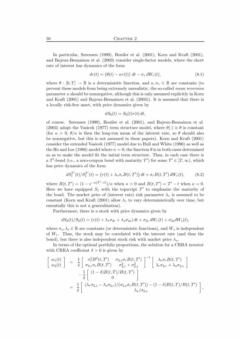
50 Chapter 2
In particular, Sørensen (1999), Bouiler et al. (2001), Korn and Kraft (2001),and Bajeux-Besnainou et al. (2003) consider single-factor models, where the shortrate of interest has dynamics of the form
dr(t) = (θ(t) − κr(t)) dt− σr dWr(t), (8.1)
where θ : [0, T ] → R is a deterministic function, and κ, σr ∈ R are constants (toprevent these models from being extremely unrealistic, the so-called mean reversionparameter κ should be nonnegative, although this is only assumed explicitly in Kornand Kraft (2001) and Bajeux-Besnainou et al. (2003)). It is assumed that there isa locally risk-free asset, with price dynamics given by
dS0(t) = S0(t)r(t) dt,
of course. Sørensen (1999), Bouiler et al. (2001), and Bajeux-Besnainou et al.(2003) adopt the Vasicek (1977) term structure model, where θ(·) ≡ θ is constant(for κ > 0, θ/κ is then the long-run mean of the interest rate, so θ should alsobe nonnegative, but this is not assumed in these papers). Korn and Kraft (2001)consider the extended Vasicek (1977) model due to Hull and White (1990) as well asthe Ho and Lee (1986) model where κ = 0; the function θ is in both cases determinedso as to make the model fit the initial term structure. Thus, in each case there isa T ′-bond (i.e., a zero-coupon bond with maturity T ′) for some T ′ ∈ [T,∞), whichhas price dynamics of the form
dST ′
1 (t)/ST ′
1 (t) =(r(t) + λrσrB(t, T ′)
)dt+ σrB(t, T ′) dWr(t), (8.2)
where B(t, T ′) = (1 − e−κ(T ′−t))/κ when κ > 0 and B(t, T ′) = T ′ − t when κ = 0.Here we have equipped S1 with the topscript T ′ to emphasize the maturity ofthe bond. The market price of (interest rate) risk parameter λr is assumed to beconstant (Korn and Kraft (2001) allow λr to vary deterministically over time, butessentially this is not a generalization).
Furthermore, there is a stock with price dynamics given by
dS2(t)/S2(t) = (r(t) + λrσ2r + λsσ2s) dt+ σ2r dWr(t) + σ2sdWs(t),
where σs, λs ∈ R are constants (or deterministic functions), and Ws is independentof Wr. Thus, the stock may be correlated with the interest rate (and thus thebond), but there is also independent stock risk with market price λs.
In terms of the optimal portfolio proportions, the solution for a CRRA investorwith CRRA coefficient δ > 0 is given by
[w1(t)w2(t)
]=
1
δ
[σ2
rB2(t, T ′) σ2,rσrB(t, T ′)
σ2,rσrB(t, T ′) σ22,r + σ2
2,s
]−1 [λrσrB(t, T ′)λrσ2,r + λsσ2,s
]
− 1
δ
[(1 − δ)B(t, T )/B(t, T ′)
0
]
=1
δ
[(λrσ2,s − λsσ2,r)/(σ2,sσrB(t, T ′)) − (1 − δ)B(t, T )/B(t, T ′)
λs/σ2,s
],

A Survey on Investment Theory 51
and w0(t) = 1−w1(t)−w2(t), where B(T, T )/B(T, T ) is interpreted as 1 if T ′ = T(note, though, that Korn and Kraft (2001) assume δ < 1). The proportion investedin the stock, λs/δσ2,s, is the same as in the case with constant interest rate, cf.(6.7). From the expression in the first line it is seen that the optimal relativeportfolio is the sum of the (generalized) classical Merton (1971) portfolio (cf. (6.5)and (6.8)), and a hedge term used to hedge the interest rate risk; this term involvesthe T ′-bond only. In particular, a high risk averter (with a large δ) will alwayshave a large proportion in the T ′-bond.
If T ′ = T (as in Sørensen (1999), Bouiler et al. (2001), and Bajeux-Besnainouet al. (2003)), then the optimal strategy has the somewhat undesirable featurethat the bond position explodes at the time horizon, as B(T ) = 0 (this does notimpose admissibility problems, though). The reason is that the volatility term ofthe bond thereby also tends to 0, so that in order to make the interest rate riskfactor stay involved the portfolio, which is necessary for effective diversificationand to benefit from the interest rate risk premium, the position in the bond mustexplode. This is of course mostly a theoretical problem. As a sort of remedy, Bouileret al. (2001) and Bajeux-Besnainou et al. (2003)) show that the optimal portfoliocan be written in terms of constant fractions by introducing another interest ratederivative, interpreted as a “rolling horizon bond” with constant time to maturity,with dynamics given by
dS3(t)/S3(t) = (r(t) + λrσ3,r) dt+ σ3,r dWr(t),
for some constant σ3,r (this derivative is redundant in the sense that it can bemimicked perfectly in the model by a dynamically managed portfolio in the locallyrisk-free asset and the T ′-bond). Then w1(t) becomes −(1−δ)/δ, w2(t) is as before,w3(t) is given by (λrσ2,s − λsσ2,r)/(δσ2,sσ3,r), and w0(t) = 1 −∑3
i=1 wi(t). Inparticular, a mutual fund consisting only of shares of the bank account, the stock,and the “rolling horizon bond” with stock proportion λs/σ2,s, “rolling horizonbond” proportion (λrσ2,s − λsσ2,r)/(σ2,sσ3,r), and the rest in the bank, could beshared by all CRRA investors; an investor with coefficient δ and time horizon Twould then invest a proportion 1/δ in this mutual fund and 1 − 1/δ in a T -bond.
Korn and Kraft (2001), on the other hand, assume that T ′ > T , which preventsthe position in the zero-coupon bond from exploding.
Brennan and Xia (2000) consider a more general two-factor model, in whichthe interest rate dynamics are given by
dr(t) = (θ(t) + Y (t) − κr(t)) dt− σr dWr(t),
where Y is a random factor with dynamics
dY (t) = (λY σY − ρY (t)) dt− σY dWY (t).
Here, λY , ρ, σY are constants (ρ should again be strictly positive), and Wr andWY are allowed to be correlated. There are two zero-coupon bonds with different

52 Chapter 2
maturities T1 < T2; their price dynamics are given by
dSTi
i (t)/STi
i (t) = (r(t) + λrσrB(t, Ti) + λY σY C(t, Ti)) dt
+ σrB(t, > Ti) dWr(t) + σYC(t, Ti) dWY (t),
i = 1, 2, where C(t, Ti)(t) = e−κ(Ti−t)/(κ(κ − ρ)) − e−ρ(Ti−t)/(ρ(κ − ρ)) + 1/(κρ).It seems necessary to assume that T1 ≥ T , although this is not done explicitly inthe paper. Moreover, as in the abovementionded papers there is a stock with pricedynamics
dS3(t)/S3(t) = (r(t) + λsσs) dt+ σs dWs(t),
where Ws is in general correlated with Wr and WY . Again, the optimal portfoliois the sum of the usual (generalized) Merton (1971) portfolio and two portfoliosconstructed so as to hedge the two state variables. However, it is shown that thismodel effectively reduces to a single-factor model in the sense that a T -bond issufficient to hedge the risk inherent in the two state variables. In other words, ifT1 = T , then the hedging portfolio is just the T -bond, and the optimal portfolioproportions in the (locally) risky assets are given by
w1
w2
w3
=
1
δΣ−1
λrσrB(t, T1) + λY σY C(t, T1)λrσrB(t, T2) + λY σY C(t, T2)
λsσs
+
(1 − 1
δ
)
010
,
where Σ is the variance matrix of the instantaneous returns. If T < T1, then twobonds and the bank account can be used to generate a T -bond.
Jensen and Sørensen (2001) extend the problem studied in Sørensen (1999) tothe general case of Gaussian term structure models without specific assumptionsabout the short rate. Furthermore, they allow for n risky assets with volatilitycoefficients that are stochastic processes. The market price of risk vector is deter-ministic, however. They obtain the general result that for a CRRA investor theoptimal asset allocation is obtained by investing a part of the wealth in the riskyassets according to the proportions given by w/δ, where w is calculated as in (6.5),and dividing the remaining proportion of wealth, 1 − 1′nw/δ, between the locallyrisk-free asset and a zero-coupon bond maturing at the time horizon T in a waythat depends on the interest rate model.
We shall briefly comment on other aspects of these papers. Sørensen (1999)focuses on implementation issues that would occur in practice, where continuoustrading in particular is impossible. In particular it is shown that one can approx-imate the solution by solving a series of short-term mean-variance optimizationproblems in terms of the short-term drift and variance of the forward price of theoptimal wealth, i.e., X(t)/ST
1 (t), where X is the wealth process of the optimalinvestment strategy.
In Bouiler et al. (2001) the optimization problem described above is actuallyonly a part of a bigger, initial problem, namely that of a (defined contribution)pension fund that seeks to optimally manage a policy, which specifies a determinis-tic continuous premium rate and a deterministic minimum annuity rate beginning

A Survey on Investment Theory 53
at the time of retirement of the policy holder (who is implicitly assumed to liveuntil the annuity runs out, i.e., mortality risk is ignored). This initial problem isformulated with the objective of maximizing the expected utility of the surplus(total assets minus liabilities) pertaining to the policy at the time of retirement,subject to the constraint that this surplus must be nonnegative. It is shown thatthis problem can be solved by short-selling and buying bonds at time 0 in sucha way that the stream of premiums and minimum annuity benefits are perfectlymatched, and then using the proceeds (which must be nonnegative in order for theproblem to have a solution) as the initial value of a portfolio, which can be man-aged independently so as to maximize the expected utility. This latter problem isthe one described above.
Korn and Kraft (2001) start out with a more general interest rate model givenby the dynamics
dr(t) = a(t, r(t)) dt− σr dWr(t),
where a : [0, T ] × R → R is an arbitrary function (satisfying certain regularityconditions). Obviously, (eq:GaussianSingleFactorShortRateDynamics) appears asa special case. They use the dynamic programming approach and prove a non-standard verification theorem applicable in this general their model. In this regardit is worth pointing out that most standard verification theorems (e.g. Fleming andRishel (1975), Fleming and Soner (1993), Yong and Zhou (1999)) rely on a certainLipschitz assumption, which is not satisfied in optimal investment problems withan unbounded interest rate.
Jensen and Sørensen (2001) also consider the situation where the investor isconstrained by the requirement that the terminal wealth must exceed a certainminimum amount, say G. This is also known as portfolio insurance. As in Coxand Huang (1989), the solution in this case is to take a fixed, long position inzero-coupon bonds that yield the payoff G and use the remaining initial wealthto buy a European call option, with strike price G, written on an asset that isformed by investing an initial amount according to the optimal relative portfolio inthe unconstrained case; the initial amount of this portfolio is determined in sucha way that the price of this option exactly equals the remaining initial wealth.Of course, if this option is not readily available, one can (in principle, at least)mimick it perfectly via a self-financing investment strategy. The authors focus onmeasuring the loss of expected utility for the investor implied by the constraint andfind that it may be quite severe if G is relatively large and the investor is relativelyrisk tolerant. They also measure the implied loss of expected utility imposed onthe investor if the wealth is invested according to a different CRRA coefficient,which may be the case if many investors with different risk attitudes enter intoa common investment pool, e.g. a pension fund. Their results indicate that suchlosses may also be quite severe, in particular for low risk averters. However, in thecase of a minimum guarantee, a high risk averter is somewhat compensated by theguarantee.
Brennan and Xia (2000) and Bajeux-Besnainou et al. (2003) discuss the optimal

54 Chapter 2
strategies and compare them with “popular advice” from certain financial advisors.In particular, both papers address an apparent puzzle pointed out by Canner et al.(1997), namely that according to many financial advisors the ratio of the bond andstock proportions in the portfolio of (locally) risky assets should increase with riskaversion, which seems to contradict the mutual fund theorems. Brennan and Xia(2000) explain that this advice is consistent with their results when the zero-couponbond(s) in the optimal portfolio are taken into account as part of the portfolio of(locally) risky assets. Bajeux-Besnainou et al. (2003) also demonstrate consistency,but from a different perspective. Note first that if one considers the T -bond as therisk-free asset (for an investor with horizon T ) and considers the mutual fund withconstant proportions in the bank account, the stock, and the “rolling horizon bond”as the risky-asset fund, then there is indeed an inconsistency when CRRA investorsare considered. However, the authors show that the optimal strategy for an investorwith HARA utility with c 6= 0 is to buy and hold a T -bond with payoff equal to−d/c and invest the remaining wealth in the optimal portfolio of a CRRA investorwith CRRA coefficient 1/c (note that a short position in this portfolio may beappropriate, as the remaining wealth after the initial purchase of the T -bond maybe negative). This means in particular that the ratio of bond and stock proportionsin the risky asset-fund is no longer constant but does indeed increase with the riskaversion.
Canestrelli and Pontini (2000) also study a pure investment problem where theshort interest rate follows the Vasicek (1977) dynamics, but in contrast to theabovementioned papers they assume that there are n risky assets modelled as inthe basic setup in Merton (1971), i.e., with price dynamics given by (6.4) withconstant coefficients. In particular, the market is incomplete. Although the Brow-nian motion W = (W1, . . . ,Wn)′ (where the components are in general correlated)is allowed to be correlated with Wr, interest rate derivatives are unattainable ingeneral, and there is in particularly no zero-coupon bonds available.
An explicit solution is obtained under certain regularity conditions on the mar-ket coefficients and the CRRA coefficient δ. In consistency with the results ofMerton (1973), the optimal investment strategy can be expressed in terms of threemutual funds: The first of these is the usual well-diversified Merton (1971) port-folio given by (6.5) and generalized, as the current interest rate is inserted at anytime; the second is determined by the vector Σ−1Γ′, where Γ is the (row) vector ofcovariances between the (instantaneuos) movements in the interest rate and the nrisky asset prices, i.e.,
Γ = (gσ1ηr1, . . . , gσnηrn),
with ηri dt = dWr(t) dWi(t), i = 1, . . . , n; the third consists of the locally risk-freeasset only. The proportion of wealth that should be invested in the Merton (1971)portfolio at time t is given by 1′nΣ−1(α− r(t)1n)/δ. This is shown to be decreasingas a function of the interest rate, which is quite natural. The purpose of the secondfund is to hedge against changes in the interest rate. The investor’s demand for thesecond and third funds depend on the market coefficients in a somewhat complex

A Survey on Investment Theory 55
manner, but it should be noted that the optimal proportions depend randomly onr(t) and t only. Moreover, the optimal proportion in the second fund tends to zeroas t tends to T , which is also quite natural.
A major drawback of the Gaussian interest rate models considered in Sørensen(1999), Canestrelli and Pontini (2000), Bouiler et al. (2001), Korn and Kraft (2001),and Jensen and Sørensen (2001), is that they allow for negative interest rates.Deelstra et al. (2000) study the pure investment problem in a setup with a Cox-Ingersoll-Ross interest rate model (Cox et al. (1985)), where r is governed by thedynamics
dr(t) = (θ − κr(t)) dt− σr
√r(t) dWr(t),
where σr, θ, κ > 0 are constants, and 2θ ≥ σ2r so that r(t) > 0, ∀t ∈ [0, T ]. The
market consists of a bank account, a T -bond, and a stock, with price dynamicsgiven by
dS0(t)/S0(t) = r(t) dt,
dS1(t)/S1(t) = (r(t) + λrσrh(t)r(t)) dt+ σrh(t)√r(t) dWr(t),
dS2(t)/S2(t) = (r(t) + λrσ2,rr(t) + λsσ2,s) dt+ σ2,r
√r(t) dWr(t) + σ2,s dWs(t),
respectively. Here, h : [0, T ] → [0,∞) is a certain differentiable function dependingon the model coefficients with h(T ) = 0. The market price of interest rate risk isλr
√r(t), whereas the market price of stock risk is λs; both λr and λs are constants.
An explicit solution is obtained in the CRRA utility case (still with δ > 0 denotingthe CRRA coefficient), under certain conditions on the risk aversion parameter.The optimal portfolio is given by the bond and stock proportions
w1(t) =λrσ2,s − λsσ2,r
δσ2,sσrh(t)+kδ(t)
h(t),
w2(t) =λs
δσ2,s,
where kδ : [0, T ] → R is a certain differentiable function, depending on δ (and themodel coefficients), with kδ(T ) = 0. It is seen that the proportion held in the stockis again the same as in the case with constant interest rate, in particular it is timeindependent. The first term in the bond proportion is similar to the first term inSørensen (1999), but the hedge term kδ(t)/h(t) is no longer constant. AlthoughlimtT (kδ(t)/h(t)) exists and is finite, the bond position once again explodes atT . However, as in Bouiler et al. (2001), the optimal portfolio can be expressed interms of portfolio proportions in the bank account, the stock, and a “rolling bond”with price dynamics given by
dS3(t)/S3(t) = (r(t) + λrσ3,rr(t)) dt+ σ3,r
√r(t) dWr(t),
for some K > 0. Then w1(t) = 0, w2 = λ2,s/σ2,s (as above), w3(t) = kδ(t)σr/σ3,r +(λrσ2,s − λsσ2,r)/(δσ2,sσ3,r), and w0(t) = 1 −∑3
i=1wi(t) (or, equivalently, w1(t) =
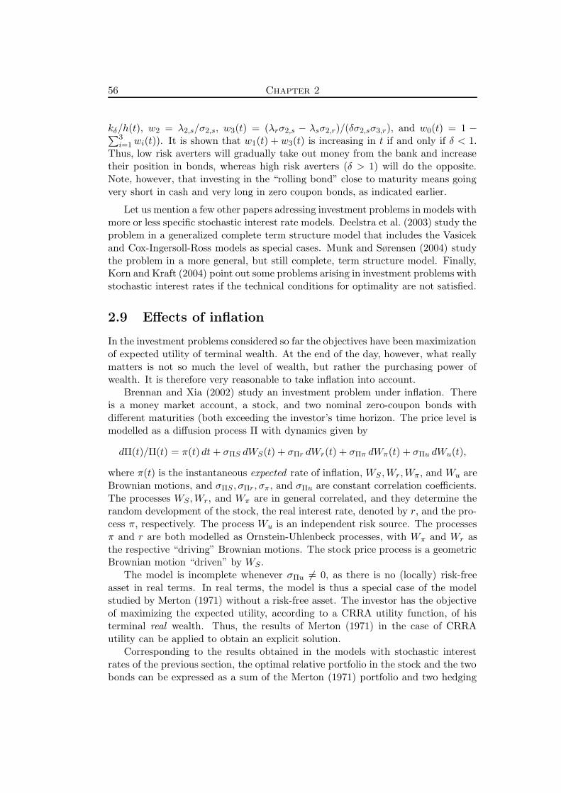
56 Chapter 2
kδ/h(t), w2 = λ2,s/σ2,s, w3(t) = (λrσ2,s − λsσ2,r)/(δσ2,sσ3,r), and w0(t) = 1 −∑3i=1 wi(t)). It is shown that w1(t) + w3(t) is increasing in t if and only if δ < 1.
Thus, low risk averters will gradually take out money from the bank and increasetheir position in bonds, whereas high risk averters (δ > 1) will do the opposite.Note, however, that investing in the “rolling bond” close to maturity means goingvery short in cash and very long in zero coupon bonds, as indicated earlier.
Let us mention a few other papers adressing investment problems in models withmore or less specific stochastic interest rate models. Deelstra et al. (2003) study theproblem in a generalized complete term structure model that includes the Vasicekand Cox-Ingersoll-Ross models as special cases. Munk and Sørensen (2004) studythe problem in a more general, but still complete, term structure model. Finally,Korn and Kraft (2004) point out some problems arising in investment problems withstochastic interest rates if the technical conditions for optimality are not satisfied.
2.9 Effects of inflation
In the investment problems considered so far the objectives have been maximizationof expected utility of terminal wealth. At the end of the day, however, what reallymatters is not so much the level of wealth, but rather the purchasing power ofwealth. It is therefore very reasonable to take inflation into account.
Brennan and Xia (2002) study an investment problem under inflation. Thereis a money market account, a stock, and two nominal zero-coupon bonds withdifferent maturities (both exceeding the investor’s time horizon. The price level ismodelled as a diffusion process Π with dynamics given by
dΠ(t)/Π(t) = π(t) dt+ σΠS dWS(t) + σΠr dWr(t) + σΠπ dWπ(t) + σΠu dWu(t),
where π(t) is the instantaneous expected rate of inflation, WS ,Wr,Wπ, and Wu areBrownian motions, and σΠS , σΠr, σπ, and σΠu are constant correlation coefficients.The processes WS ,Wr, and Wπ are in general correlated, and they determine therandom development of the stock, the real interest rate, denoted by r, and the pro-cess π, respectively. The process Wu is an independent risk source. The processesπ and r are both modelled as Ornstein-Uhlenbeck processes, with Wπ and Wr asthe respective “driving” Brownian motions. The stock price process is a geometricBrownian motion “driven” by WS .
The model is incomplete whenever σΠu 6= 0, as there is no (locally) risk-freeasset in real terms. In real terms, the model is thus a special case of the modelstudied by Merton (1971) without a risk-free asset. The investor has the objectiveof maximizing the expected utility, according to a CRRA utility function, of histerminal real wealth. Thus, the results of Merton (1971) in the case of CRRAutility can be applied to obtain an explicit solution.
Corresponding to the results obtained in the models with stochastic interestrates of the previous section, the optimal relative portfolio in the stock and the twobonds can be expressed as a sum of the Merton (1971) portfolio and two hedging

A Survey on Investment Theory 57
portfolios aimed at hedging the risks pertaining to real interest rate and the rateof inflation. Akin to the result obtained by Karatzas et al. (1991) in the specialcase with totally unhedgeable coefficients, the optimal portfolio does not dependon σΠu, the volatility corresponding to the totally unhedgeable risk, i.e., this riskis ignored. The parts of the inflation risk that can be partially hedged should betreated similarly as other types of risks in a standard Brownian motion model withconstant coefficients.
2.10 Some concluding remarks
We end this survey by offering a few concluding remarks. However, most of theabovementioned results are discussed at length by the authors who have obtainedthem, and we shall not go into a detailed and exhaustive discussion.
For long-term investors, such as pension savers, the classical single-period ap-proach is insufficient; multi-period (with many periods) or continuous-time modelsare called for. In particular, continuous-time models with Brownian motions as ba-sic building blocks, which are the most widely used ones in the modern literature,can often yield explicit results on optimal investment; Merton’s results constitutethe primary example.
Certain specific aspects concerning pension saving should be taken into account.For example, minimum guarantees are often involved, and the long-term natureof pension schemes calls for models with a stochastic interest rate in order tobe sufficiently realistic. However, models with a constant interest rate can beconsidered very reasonable, even with long time horizons, if the interest rate isinterpreted as the real interest rate, rather than the nominal one, and the wealthand the asset prices are taken to be denominated in real terms, as they arguablyshould be (see also Section 2.9). With this interpretation the assumption is that thereal interest rate, rather than the nominal one, is constant, which is more plausible.
As pointed out, the choice of utility function plays an extremely importantrole for the optimal strategy. In particular, what is optimal cannot be statedwithout reference to the underlying utility function employed. This also goes for themany interesting problems that have been left out of this survey. One particularlynice and simple class of utility functions, which (as we have seen above) has verydesirable features, is the class of CRRA utility functions, possibly extented to allowfor minimum guarantees. It is therefore no coincidence that these utility functionsare the most widely used ones in the literature.


Chapter 3
Optimal Bonus Strategies inLife Insurance: The MarkovChain Interest Rate Case
Sections 3.1-3.5 of this chapter constitute an adapted version of Nielsen(2005), with only minor corrections and modifications. Section 3.6 hasbeen added for this thesis and thus does not appear in Nielsen (2005).
We study the problem of optimal redistribution of surplus in life and pension in-surance when the interest rate is modelled as a continuous-time Markov chain witha finite state space. We work with traditional participating life insurance policieswith payments consisting of a specified contractual payment stream and an un-specified additional bonus payment stream. Our model allows for interest ratesbelow the technical interest rate. We apply stochastic control techniques in oursearch for optimal strategies, and we prove the dynamic programming principlefor our particular type of problem. Furthermore, we state and prove a verificationtheorem and obtain an explicit solution that leads to a characterization of optimalstrategies, indicating that some widely used redistribution schemes are suboptimal.
3.1 Introduction
A participating life or pension insurance contract specifies, at the time of issue, apremium plan and a fixed stream of (so-called) guaranteed benefits, both dependingrandomly only on the future course of life of the insured. On top of this the insuredis entitled to additional bonus benefits, which, on the contrary, are determined bythe company currently during the policy term as the systematic (portfolio) surplusemerges, as a consequence of the fact that all policies are charged (implicitly) witha safety loading.
59

60 Chapter 3
The bonus payments typically contribute significantly to the total benefits andthus constitute one of the most important decision problems in traditional life andpension insurance, because it is up to the company to decide on the dividend/bonusplan (the distinction between dividends and bonuses is unimportant at this pointand will be explained later, although we make clear that dividends go to the insured,not to owners or shareholders). Two concerns are involved: On the one hand,the company is urged to hand out dividends to the insured on a regular basis,partly to satisfy current customers (the insured) and perhaps even try to gainshares in the competitive market of the insurance business, and partly by legislativedemands. On the other hand, the companies must see to it that they do not handout more than they can afford, that is, they should always be able to meet allfuture obligations. It should be noted that dividends and bonuses, which havebeen credited/paid out to a policy at one stage, cannot be reclaimed later on.
The purpose of this chapter is to formulate and solve the problem of designingan optimal dividend plan as a control problem, taking into account the abovemen-tioned concerns, in a stochastic interest rate environment. The paper is to someextent related to the comprehensive existing literature on optimal investment andconsumption in continuous-time models, initiated by the classical papers Merton(1969) and Merton (1971). Virtually countless different variations and general-izations of investment/consumption problems have been studied since then, see,e.g. Duffie (1996), Ch. 9, or Karatzas and Shreve (1998), Sec. 3.11, for extensivesurveys.
The problem studied in this paper differs from the vast majority of this litera-ture in several respects. The interest rate (intensity) is modelled as a continuous-time Markov chain with a finite state space, and we consider the corresponding(locally) risk-free asset as the only investment opportunity and thus deal with theconsumption/dividend aspect only. This means that the process under control isnot a diffusion, but a PDP (piecewise deterministic process). Furthermore, our“agent” faces a certain non-hedgeable stream of positive and negative payments,but has no initial endowment.
Our objective (formulated in Section 3.3) constitutes another distinction, asit resembles the type of objectives employed in singular control problems. This,combined with the fact that our purpose is to find an optimal dividend strategy,leads to a connection to the class of problems known as dividend optimizationproblems, see e.g. Radner and Shepp (1996), or Taksar (2000) for a survey focusingon insurance companies. Such problems, aiming at maximizing (in some sense)the value of future dividends to shareholders for a firm with some initial reserveand a certain stochastic revenue process (typically a diffusion) through control ofdividends and possibly risk exposure and/or investments, are often formulated assingular control problems. However, the connection is not as apparent as it mayseem. Firstly, dividends play an entirely different role in this paper (as mentionedabove). Secondly, our “revenue process” is not a diffusion, and, as we shall see, theoptimal control process therefore need not have a singular component. Thirdly, ourproblem has a known, finite horizon, whereas the time horizon in most dividend

Optimal Bonus Strategies in Life Insurance 61
optimization problems is either infinity or the (random) time of ruin.
Lakner and Slud (1991) study a problem akin to ours: They consider an agent,who only invests in a locally risk-free asset with an interest rate intensity that isadapted to a point process, and who seeks to optimize his consumption stream.However, the objective has a distinctly different form from ours, and there are noexogenous payment streams involved.
There exists a literature on optimization problems of various kinds within lifeinsurance and/or pension funding. Optimal contribution (premium) rates for pen-sion funds with defined benefit (DB) schemes are studied in Haberman and Sung(1994) and Chang et al. (2003). This problem is extended to include the problemof optimal asset allocation in Cairns (2000), Josa-Fombellida and Rincon-Zapatero(2001) and Taylor (2002). As for the contribution rates, the objectives in thosepapers are to minimize a certain loss function measuring (in various ways) thetotal sum of squared distances to certain targets of the controllable contributionrate and the aggregate fund level. A different approach, also within DB models,is taken in Haberman (1994) and Haberman and Wong (1997), where the aim isto find optimal time periods for distributing surpluses or deficits in the fund levelthrough adjustment of the contribution rates.
For defined contribution schemes optimal investment strategies constitute themain issue, and this has been studied in Bouiler et al. (2001), Deelstra et al.(2003), Devolder et al. (2003), Vigna and Haberman (2001) and Haberman andVigna (2002).
The present study is distinct from all the abovementioned: Firstly, we considerthe dividend problem only, as we take the returns from investments as exoge-nously given (although stochastic). Secondly, our modelling approach is different,as we consider an individual (generic) policy with certain contractual paymentsand consider the associated surplus process throughout the policy term, whereasthe abovementioned papers largely take more of a bird’s eye view and consider thedynamics of the aggregate fund level without bringing the life history stochasticsof the individual policies to the surface. Thirdly, our objective is (subjective) valuemaximization, not risk minimization.
The rest of the chapter is organized as follows: We briefly introduce the basicsetup in Section 3.2 and then go on to state the optimal stochastic control problemin Section 3.3. We present theoretical results in Section 3.4 and obtain an explicitcharacterization of optimal dividend strategies. Section 3.5 contains main discus-sions and general conclusions. Finally, Section 3.6 contains generalizations of theresults.
A quick word on notation: Integrals of the form∫[t,t′] fs dAs for functions or
processes (f predictable, A FV and right-continuous) are interpreted as ft∆At +∫(t,t′ ] fs dAs, with ∆At = At if As is not defined for s < t. Correspondingly,∫(t,t′) fs dAs means limτt′
∫(t,τ ] fs dAs and so on.

62 Chapter 3
3.2 Basics
A. The insurance policy and the contractual payments.We work throughout on the basis of the general model in Norberg (1999), which is abasic reference for notions such as surplus, bonus and dividends, although we makespecializations for the purpose of our study. In this section we briefly recapitulatethe notions and results used in the following, referring to Norberg (1999) for detailsand discussions.
Consider a generic multi-state life insurance policy issued at time 0 and termi-nating at time T > 0. The state of the policy at time t ∈ [0, T ] is denoted by Zt,and Z = (Zt)t∈[0,T ] is taken to be a right-continuous Markov process defined onsome probability space (Ω,F ,P), with a finite state space Z = 1, . . . , k and witha finite number of jumps in [0, T ]. It is assumed that the initial state is 1, Z0 = 1.
The contractual payments associated with the policy, i.e. premiums and guar-anteed benefits, are represented by a stochastic payment process B = (Bt)t∈[0,T ]
specifying the accumulated payments from the company to the insured, that is, Bt
denotes benefits less premiums payable in [0, t], t ∈ [0, T ]. It is assumed that B hasa form that allows of continuous payments during sojourns in policy states as wellas lump sum payments at a finite number of fixed times and in connection withjumps between policy states. Thus, B has an absolutely continuous componentand a pure jump component, and all randomness associated with the paymentsdBt in a small time interval (t, t + dt] is due to the (random) behaviour of Z inthat interval.
Even though this formalization of the payment process opens up for a wide rangeof insurance types, the problem that we deal with in this paper is more relevantfor some types of insurance than others. Typically we have in mind a pensionscheme with the following characteristics: The policyholder pays a level premiumcontinuously for a certain number of years from the time of issue, possibly untilthe time of retirement, and receives a continuous life annuity, possibly temporary,commencing at a specific time (e.g. the time of retirement); with all payments beingcontingent on the policyholder being alive.
The payment process B must satisfy the actuarial equivalence principle undera technical first order model that lays down a (technical) interest rate r∗ ∈ R anda (technical) distribution of Z. We assume for simplicity that the distribution ofZ under the first order model coincides with its distribution under P, which, inthe terminology of Norberg (1999), corresponds to the second order model. Thisassumption can be justified by the fact that the interest rate risk is considerablylarger than the risk connected to systematic changes in, say, mortality, for pensionschemes as the one outlined above. Thus, upon introducing the first order state-wise (prospective) reserves V ∗j, j ∈ Z, in this setting given by
V ∗jt = E
(∫
(t,T ]e−(τ−t)r∗ dBτ
∣∣∣∣∣Zt = j
),
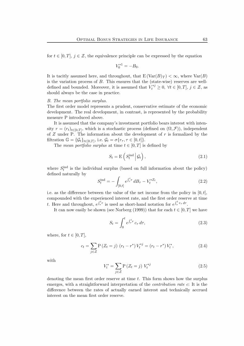
Optimal Bonus Strategies in Life Insurance 63
for t ∈ [0, T ], j ∈ Z, the equivalence principle can be expressed by the equation
V ∗10 = −B0.
It is tacitly assumed here, and throughout, that E (Var(B)T ) < ∞, where Var(B)is the variation process of B. This ensures that the (state-wise) reserves are well-defined and bounded. Moreover, it is assumed that V ∗j
t ≥ 0, ∀t ∈ [0, T ], j ∈ Z, asshould always be the case in practice.
B. The mean portfolio surplus.The first order model represents a prudent, conservative estimate of the economicdevelopment. The real development, in contrast, is represented by the probabilitymeasure P introduced above.
It is assumed that the company’s investment portfolio bears interest with inten-sity r = (rt)t∈[0,T ], which is a stochastic process (defined on (Ω,F)), independentof Z under P. The information about the development of r is formalized by thefiltration G = Gtt∈[0,T ], i.e. Gt = σrτ , τ ∈ [0, t].
The mean portfolio surplus at time t ∈ [0, T ] is defined by
St = E(Sind
t
∣∣∣Gt
), (2.1)
where Sindt is the individual surplus (based on full information about the policy)
defined naturally by
Sindt = −
∫
[0,t]e∫ t
τr dBτ − V ∗Zt
t , (2.2)
i.e. as the difference between the value of the net income from the policy in [0, t],compounded with the experienced interest rate, and the first order reserve at time
t. Here and throughout, e∫ t
sr is used as short-hand notation for e
∫ t
srτ dτ .
It can now easily be shown (see Norberg (1999)) that for each t ∈ [0, T ] we have
St =
∫ t
0e∫ t
τr cτ dτ, (2.3)
where, for t ∈ [0, T ],
ct =∑
j∈Z
P (Zt = j) (rt − r∗)V ∗jt = (rt − r∗)V ∗
t , (2.4)
withV ∗
t =∑
j∈Z
P (Zt = j) V ∗jt (2.5)
denoting the mean first order reserve at time t. This form shows how the surplusemerges, with a straightforward interpretation of the contribution rate c: It is thedifference between the rates of actually earned interest and technically accruedinterest on the mean first order reserve.

64 Chapter 3
Equivalently, from (2.1) we easily obtain
St = −∫
[0,t]e∫ t
τr dbτ −
∫
(t,T ]e−(τ−t)r∗dbτ ,
where b is defined by bt = E(Bt) , t ∈ [0, T ]. Thus, the mean portfolio surplusis nothing but the difference between the compounded value of past net incomeand the present value of future net outgoes (evaluated on the first order basis)corresponding to the (artificial) deterministic payment stream b.
C. The dividend reserve.The surplus (or a part of it) is repaid to the insured by crediting dividends to hisor her account. The stream of dividends is represented by the stochastic processD = (Dt)t∈[0,T ], and as for the payment process B, Dt denotes the accumulateddividends during [0, t], t ∈ [0, T ]. Dividends can only be credited on the basisof the information that is currently known, and since we work with the meanportfolio surplus we must therefore require that D be G-adapted. This means thatD represents the mean dividends per policyholder in the entire portfolio (includingthose who have died). Thus, the policy that we consider should be thought of asa truly generic “mean” policy representing the portfolio, not as a specific policy.By taking this approach we avoid having to deal with policy state variables in thecontrol problem addressed below.
Furthermore, dividends must be non-negative and cannot be reclaimed oncethey have been credited, so D must be non-negative and non-decreasing. Finally,D is taken to be right-continuous.
The dividend reserve Ut at time t ∈ [0, T ] is defined as the value at time t ofpast contributions less dividends, compounded with interest, i.e.
Ut =
∫
[0,t]e∫ t
τr (cτ dτ − dDτ ). (2.6)
Credited dividends may be used in various ways and need not be paid out immedi-ately. The actual payouts, in turn, are called bonuses. In some simple cases, e.g. ifdividends are paid out currently as they are credited, then the distinction betweendividends and bonus payments is not important. In most cases it is, however, andthe distribution and repayment of surplus can then be viewed as a two-step proce-dure: First, dividends are determined and distributed among the policies accordingto some dividend scheme. Then, according to a bonus scheme, it is decided how thedistributed dividends are transformed into bonus payments. We refer to Norberg(1999, 2001) for more detailed discussions on this quite flexible system.
From (2.6) it is easily seen that U develops as
U0 = −D0, (2.7)
dUt = rtUt dt+ ct dt− dDt, (2.8)
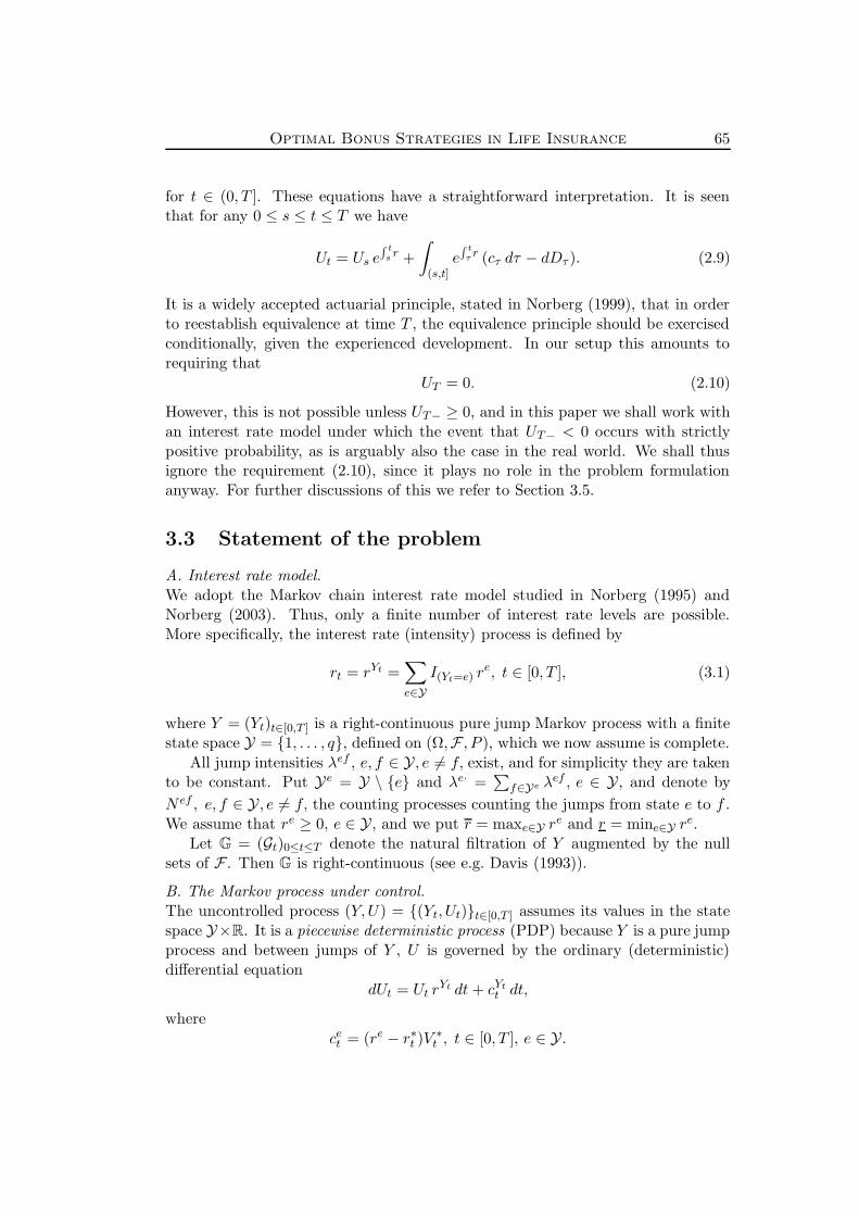
Optimal Bonus Strategies in Life Insurance 65
for t ∈ (0, T ]. These equations have a straightforward interpretation. It is seenthat for any 0 ≤ s ≤ t ≤ T we have
Ut = Us e∫ t
sr +
∫
(s,t]e∫ t
τr (cτ dτ − dDτ ). (2.9)
It is a widely accepted actuarial principle, stated in Norberg (1999), that in orderto reestablish equivalence at time T , the equivalence principle should be exercisedconditionally, given the experienced development. In our setup this amounts torequiring that
UT = 0. (2.10)
However, this is not possible unless UT− ≥ 0, and in this paper we shall work withan interest rate model under which the event that UT− < 0 occurs with strictlypositive probability, as is arguably also the case in the real world. We shall thusignore the requirement (2.10), since it plays no role in the problem formulationanyway. For further discussions of this we refer to Section 3.5.
3.3 Statement of the problem
A. Interest rate model.We adopt the Markov chain interest rate model studied in Norberg (1995) andNorberg (2003). Thus, only a finite number of interest rate levels are possible.More specifically, the interest rate (intensity) process is defined by
rt = rYt =∑
e∈Y
I(Yt=e) re, t ∈ [0, T ], (3.1)
where Y = (Yt)t∈[0,T ] is a right-continuous pure jump Markov process with a finitestate space Y = 1, . . . , q, defined on (Ω,F , P ), which we now assume is complete.
All jump intensities λef , e, f ∈ Y, e 6= f, exist, and for simplicity they are takento be constant. Put Ye = Y \ e and λe· =
∑f∈Ye λef , e ∈ Y, and denote by
N ef , e, f ∈ Y, e 6= f, the counting processes counting the jumps from state e to f .We assume that re ≥ 0, e ∈ Y, and we put r = maxe∈Y r
e and r = mine∈Y re.
Let G = (Gt)0≤t≤T denote the natural filtration of Y augmented by the nullsets of F . Then G is right-continuous (see e.g. Davis (1993)).
B. The Markov process under control.The uncontrolled process (Y,U) = (Yt, Ut)t∈[0,T ] assumes its values in the statespace Y×R. It is a piecewise deterministic process (PDP) because Y is a pure jumpprocess and between jumps of Y , U is governed by the ordinary (deterministic)differential equation
dUt = Ut rYt dt+ cYt
t dt,
where
cet = (re − r∗t )V∗t , t ∈ [0, T ], e ∈ Y.
66 Chapter 3
Control of the dividend reserve process is carried out through the dividend processD, yielding the (stochastic) dynamics (2.8).
A key reference in the theory of control of PDP’s is Davis (1993), which, forthis chapter, however, has served primarily as a source of inspiration, because theproblem at hand does not quite fit into its framework (e.g. due to the general formof D).
We denote by E the state space for the triple process (t, Yt, Ut)t∈[0,T ], that is,E = [0, T ]×Y ×R. For notational convenience we also define E0 = [0, T )×Y ×R.
Note that the policy process Z no longer plays any role, because we work withthe mean portfolio surplus.
C. Objective.We want to design a control strategy that is optimal in some sense, and to this endwe wish to maximize
E
(∫
[0,T )e−
∫ s
0r dDs + e−
∫ T
0rψ(UT−)
), (3.2)
the sum of the expected discounted dividends and the expected discounted “utility”of the dividend reserve immediately before T as measured by some concave andstrictly increasing function ψ : R → R. Note that we only integrate over [0, T )because any terminal dividend lump sum ∆DT is taken directly from UT− andthus (indirectly) measured by ψ. In other words, all control action takes place in[0, T ). We refer to Section 3.5 for a discussion of this objective as well as principlesregarding UT−.
3.4 Control theory
A. Dynamic programming framework.We apply the method of dynamic programming, and to this end we need to considereach point (t, e, u) ∈ E0 as an (imaginary) initial point for the controlled process.For technical reasons (needed in the proof of the dynamic programming principle,Theorem 3.4.5 below) we set up the dynamic programming framework rigorously,as in Fleming and Rishel (1975) or Yong and Zhou (1999).
For any (t, e) ∈ [0, T )×Y we define D(t, e) as the set of all 5-tuples (Ω,F ,P, Y,D)such that (Ω,F ,P) is a complete probability space, Y = (Ys)s∈[t,T ] is a continuous-time Markov chain defined on (Ω,F ,P) with state space Y and transition intensitiesλef , e, f ∈ Y, e 6= f, and with Yt = e (P-a.s.), and D = (Ds)s∈[t,T ] : Ω × [t, T ] →[0,∞) is a measurable, G-adapted, right-continuous and increasing process withE(t,e) (DT ) <∞. Here, G = (Gs)s∈[t,T ] denotes the filtration generated by Y (aug-mented by all the P-null sets of F), r = (rs)s∈[t,T ] is defined as in (3.1) on [t, T ],and E(t,e) (·) is the expectation operator corresponding to P, equipped with thesubscript (t, e) to emphasize the initial point.
For notational simplicity we shall usually write D ∈ D(t, e) as shorthand for(Ω,F ,P, Y,D) ∈ D(t, e) when no confusion can arise. Now, for any (t, e, u) ∈ E 0

Optimal Bonus Strategies in Life Insurance 67
and any D ∈ D(t, e) we define
U(t,e,u,D)t′ = ue
∫ t′
tr +
∫
[t,t′]e∫ t′
τr(cτ dτ − dDτ ), t
′ ∈ [t, T ], (4.1)
i.e. the dividend reserve at time t′ corresponding to the starting point (t, e, u) andthe dividend strategy D (see (2.9)), and
ΦD(t, e, u) = E(t,e)
(∫
[t,T )e−
∫ st
r dDs + e−∫ Tt
r ψ(U
(t,e,u,D)T−
)). (4.2)
In addition we put ΦD(T, e, u) = ψ(u), (e, u) ∈ Y×R, and we have thereby definedthe performance function ΦD : E → R. Note that in (4.1) u acts only as a
parameter, and in (4.2) it therefore appears only in U(t,e,u,D)T− , not in the subscript
of the expectation operator.
We define correspondingly the value function Φ : E → R by
Φ(t, e, u) = supD∈D(t,e)
ΦD(t, e, u), (t, e, u) ∈ E0,
which is well defined by Assumption 3.4.1 below, and Φ(T, e, u) = ψ(u), (e, u) ∈Y × R. For a given starting point (t, e, u) ∈ E0 the objective is to find an optimalcontrol, i.e. a control D ∈ D(t, e) satisfying
Φ(t, e, u) = ΦD(t, e, u),
and for our original problem the objective is thus expressed by letting t = 0, e = Y0
and u = 0.
Assumption 3.4.1 We assume throughout that
(i) ψ ∈ C1(R),
(ii) there exists a u0 ∈ R such that ψ′(u0) > 1,
(iii) L := limu→−∞ ψ′(u) <∞.
Condition (i) can be weakened, but it is enforced because it simplifies the resultsand proofs in the following. Condition (ii) ensures that the control problem is wellposed: Under this condition it is fairly easy to show that the value function is finite.Conversely, if it is not fulfilled, then any control D ′ ∈ D(t, e) can be dominated bya “larger” one, that is, if we define D ′′ := D′ +K for some constant K > 0 thenΦD′′
(t, e, u) ≥ ΦD′
(t, e, u), leading to a highly counter-intuitive dividend strategy.The interpretation of this condition is that ultimate losses must not be punishedtoo lightly. Condition (iii) is purely technical and is needed in certain proofs in thefollowing. This condition ensures that ψ is Lipschitz continuous (with Lipschitz

68 Chapter 3
constant L). However, as we shall see, it has no effect on the optimal strategies (ifproperly applied).
We shall need the following technical result. For t ∈ [0, T ], let A[t, T ] denotethe space of right-continuous functions d : [t, T ] → Y, equipped with the σ-algebragenerated by the coordinate projections (d 7→ ds)d∈A[t,T ]s∈[t,T ].
Lemma 3.4.2 Let D ∈ D(t, e) for fixed (t, e) ∈ [0, T )×Y. There exists a measur-able mapping η : [t, T ] ×A[t, T ] → [0,∞) such that
Ds(ω) = η (s, Y·∧s(ω)) , ∀s ∈ [t, T ], P − a.s.
Proof. Since D is G-adapted, there exists for each s ∈ [t, T ] a measurable mappingηs : A[t, T ] → [0,∞) such that Ds = ηs(Y·∧s) P − a.s. Now, for n ≥ 1, puttk = t+ (T − t)k/2n, k = 0, . . . , 2n, and define ηn : [t, T ] ×A[t, T ] → [0,∞) by
ηn(s, d) = 1t(s)ηt(d) +
2n∑
k=1
1(tk−1 ,tk](s)ηtk(d), (s, d) ∈ [t, T ] ×A[t, T ].
Each ηn is clearly measurable, and we have Dtk = ηn(tk, Y·∧tk), ∀k = 0, . . . , 2n, P−a.s. Since D is also right-continuous, the mapping η : [t, T ]×A[t, T ] → [0,∞) givenby
η(s, d) = limn→∞
ηn(s, d), (s, d) ∈ [t, T ] ×A[t, T ],
is well defined and fulfills the assertion. 2
B. Basic properties of the value function.The following results are hardly surprising.
Proposition 3.4.3 For any (t, e) ∈ [0, T ] ×Y, Φ(t, e, ·) is increasing and concaveas a function of u ∈ R.
Proof. Let (t, e) ∈ [0, T )×Y (for t = T the assertions are obvious). It is obvious thatΦ(t, e, ·) is increasing. To prove concavity, let u′ < u′′ ∈ R, and let D′, D′′ ∈ D(t, e).Let 0 ≤ γ ≤ 1, and put
uγ = γu′ + (1 − γ)u′′.
We now claim that there exists a Dγ ∈ D(t, e) such that
ΦDγ
(t, e, uγ) ≥ γΦD′
(t, e, u′) + (1 − γ)ΦD′′
(t, e, u′′). (4.3)
Then, for any ε > 0, by choosing D′ and D′′ such that ΦD′
(t, e, u′) ≥ Φ(t, e, u′)− εand ΦD′′
(t, e, u′′) ≥ Φ(t, e, u′′) − ε, the inequality (4.3) yields
Φ(t, e, uγ) ≥ γΦ(t, e, u′) + (1 − γ)Φ(t, e, u′′) − ε,
from which concavity follows because ε is arbitrary.

Optimal Bonus Strategies in Life Insurance 69
To prove the existence of Dγ ∈ D(t, e) fulfilling (4.3) we may, by suitable use ofLemma 3.4.2, assume that the underlying probability spaces and Y -processes cor-responding to D′ and D′′ are identical. Thus, we can define Dγ on this probabilityspace by
Dγ = γD′ + (1 − γ)D′′.
It is now easily seen that
U(t,e,uγ ,Dγ)T− = γU
(t,e,u′,D′)T− + (1 − γ)U
(t,e,u′′,D′′)T− ,
and by concavity of ψ we therefore get (4.3). 2
Proposition 3.4.4 For any (t, e) ∈ [0, T ] × Y and any D ∈ D(t, e), Φ(t, e, ·) andΦD(t, e, ·) are Lipschitz continuous as functions of u ∈ R.
Proof. Let (t, e) ∈ [0, T ) × Y (for t = T the assertions are obvious, cf. Assump-tion 3.4.1). Let u′ < u′′ ∈ R, and let D ∈ D(t, e). We have∣∣ΦD(t, e, u′′) − ΦD(t, e, u′)
∣∣ ≤∣∣∣E(t,e)
(e−
∫ T
tr[ψ(U
(t,e,u′′,D)T− ) − ψ(U
(t,e,u′,D)T− )
])∣∣∣
≤ E(t,e)
∣∣∣ψ(U(t,e,u′′,D)T− ) − ψ(U
(t,e,u′,D)T− )
∣∣∣
≤ LeTr|u′′ − u′|,which shows that ΦD(t, e, ·) is Lipschitz continuous with Lipschitz constant LeT r.Since D ∈ D(t, e) was arbitrary, we conclude that the same goes for Φ(t, e, ·). 2
Measurability of Φ follows from the fact that also Φ(·, e, u) is continuous on[0, T ) for any (e, u) ∈ Y × R. We choose to omit the proof of this, however, sinceit is tedious and technically rather complicated, and since continuity in t on [0, T )is intuitively obvious.
C. The dynamic programming principle.The following theorem establishes the dynamic programming principle (DPP) forthe control problem considered in this chapter. A rigorous proof covering thistype of problem has not been found in the literature. The proof, which is rathertechnical, is highly inspired by the proof of Yong and Zhou (1999), Theorem 4.3.3.
Theorem 3.4.5 For any (t, e, u) ∈ E0 and any t′ ∈ [t, T ],
Φ(t, e, u) = supD∈D(t,e)
E(t,e)
(∫
[t,t′)e−
∫ s
trdDs + e−
∫ t′
tr Φ(t′, Yt′ , U
(t,e,u,D)t′−
)).
Proof. Let (t, e, u) ∈ E0 and t′ ∈ [t, T ]. To ease notation we write E instead ofE(t,e) throughout this proof. For any D ∈ D(t, e),
ΦD(t, e, u) = E
(∫
[t,t′)e−
∫ s
trdDs
)
+ E
(e−
∫ t′
tr E
(∫
[t′,T )e−
∫ s
t′rdDs + e−
∫ T
t′rψ(U
(D,t,e,u)T−
) ∣∣∣∣∣Gtt′
)).

70 Chapter 3
We now claim that we almost surely have
E
(∫
[t′,T )e−
∫ st′
rdDs + e−∫ T
t′rψ(U
(D,t,e,u)T−
) ∣∣∣∣∣Gtt′
)≤ Φ
(t′, Yt′ , U
(D,t,e,u)t′−
), (4.4)
leading to
ΦD(t, e, u) ≤ E
(∫
[t,t′)e−
∫ st
rdDs + e−∫ t′
trΦ(t′, Yt′ , U
(D,t,e,u)t′−
)),
which in turn implies the inequality “≤”. Although (4.4) may seem intuitively veryreasonable, it takes a few lines of technicalities to prove it with some degree of rigor:Since Y and D are right-continuous, there exists a set Ω0 ∈ F with P (Ω0) = 1such that the following holds true: For any fixed ω0 ∈ Ω0, Y and D are (almostsurely) deterministic on [t, t′] under P
(· | Gt
t′)(ω0), where P
(· | Gt
t′)
denotes a regu-lar conditional probability (of P) given G t
t′ . And furthermore, by Lemma 3.4.2 wecan deduce that under P
(· | Gt
t′)(ω0), the process D restricted to [t′, T ] is adapted
to the process Y restricted to [t′, T ], and the latter is a continuous-time Markovprocess starting in the state Yt′(ω0) and otherwise inheriting the distributionalproperties of Y . Thus, (Ω,P
(· | Gt
t′)(ω0),F , Y |[t′,T ], D) ∈ D(t′, Yt′(ω0)). Further-
more, we have
U(D,t,e,u)T− = U
(D,t′,Yt′ ,U(D,t,e,u)
t′−)
T− , (4.5)
with Yt′ and U(D,t,e,u)t′− being deterministic under (Ω,P
(· | Gt
t′)(ω0),F). Substi-
tuting (4.5) into the left hand side of (4.4) and using the rule E(· | Gt
t′)(ω0) =
EP( · |Gtt′)(ω0) (·) yields the desired inequality.
Conversely, for any ε > 0, by Proposition 3.4.4 there exists δ > 0 such that forany e ∈ Y and u1, u2 ∈ R with |u1 − u2| < δ we have∣∣ΦD(t′, e, u1) − ΦD(t′, e, u2)
∣∣+∣∣Φ(t′, e, u1) − Φ(t′, e, u2)
∣∣ ≤ ε, ∀D ∈ D(t′, e).
Let (In)n≥1 be a partition of R with each In being an interval of length m(In) ≤ δ.Now choose, for each n ≥ 1, a un ∈ In. For any e ∈ Y and n ≥ 1 there existsDe,n ∈ D(t′, e) such that
ΦDe,n
(t′, e, un) ≥ Φ(t′, e, un) − ε.
Thus, for any u ∈ In we have
ΦDe,n
(t′, e, u) ≥ ΦDe,n
(t′, e, un) − ε ≥ Φ(t′, e, un) − 2ε ≥ Φ(t′, e, u) − 3ε.
For each e ∈ Y and n ≥ 1 there exists by Lemma 3.4.2 a measurable mappingηe,n : [t′T ] × A[t′, T ] → [0,∞) such that De,n
s = ηe,n(s, Y·∧s), P − a.s. Now, takeany control D ∈ D(t, e), and define a new control D ∈ D(t, e) by Ds = Ds for s < t′
and
Ds = Dt′− +∑
f∈Y
∑
n≥1
1(e,In)
((Yt′ , U
(D,t,e,u)t′ )
)ηe,n (s, (Yτ∧s)t′≤τ≤T ) , t′ ≤ s ≤ T.

Optimal Bonus Strategies in Life Insurance 71
This new control is seen to be admissible, and
Φ(t, e, u) ≥ ΦD(t, e, u)
= E
(∫
[t,T )e−
∫ s
trdDs + e−
∫ T
trψ(U
(D,t,e,u)T−
))
= E
(∫
[t,t′)e−
∫ s
trdDs
)
+ E
(e−
∫ t′
tr E
(∫
[t′,T )e−
∫ st′
rdDs + e−∫ Tt′
rψ(U
(D,t,e,u)T−
) ∣∣∣∣∣Gtt′
)).
Now, with arguments similar to the ones used in the proof of (4.4), we almost surelyhave
E
(∫
[t′,T )e−
∫ s
t′rdDs + e−
∫ T
t′rψ(U
(D,t,e,u)T−
) ∣∣∣∣∣Gtt′
)≥ Φ(t′, Yt′ , U
(D,t,e,u)t′− ) − 3ε,
and thus, by arbitraryness of ε > 0,
Φ(t, e, u) ≥ E
(∫
[t,t′)e−
∫ st
rdDs + e−∫ t′
trΦ(t′, Yt′ , U
(D,t,e,u)t′−
)),
This proves the inequality “≥”, because D ∈ D(t, e) was arbitrary. 2
D. Variational inequalities and heuristically optimal controls.The value function can be viewed as a function with q components, namely thestate-wise value functions Φe(·, ·) = Φ(·, e, ·) : [0, T ]×R → R, e ∈ Y, correspondingto the different states in Y. Dropping the generic argument (t, u) to ease notation,the HJB equation of dynamic programming becomes a system of variational in-equalities for these functions, which can be expressed (using the notation φ for thegeneric function argument) by
0=max
∂
∂tφe − φe re +
∂
∂uφe (reu+ cet ) +
∑
f∈Ye
λef (φf − φe), 1 − ∂
∂uφe
, e ∈ Y,
(4.6)with the boundary condition
φe(T, u) = ψ(u), (e, u) ∈ Y × R. (4.7)
A heuristic argument for this system of equations goes as follows: Assume for amoment that only absolutely continuous dividend processes are allowed, such thatany control is of the form dDt = δt dt for some dividend rate process δ. Then,assuming furthermore that Φ ∈ C1(E0), the dynamic programming principle leads

72 Chapter 3
to the HJB equation
0 =∂
∂tΦe(t, u) − Φe(t, u)re +
∂
∂uΦe(t, u) (reu+ cet )
+∑
f∈Ye
λef (Φf (t, u) − Φe(t, u)) + supδ≥0
(δ − ∂
∂uΦe(t, u)δ
). (4.8)
It is seen that if ∂∂uΦYt(t, Ut) > 1, the optimum is obtained by putting δt = 0.
However, if ∂∂uΦYt(t, Ut) < 1 then no optimum exists, but obviously δ should be
chosen as large as possible.Now, allowing dividend strategies that are not absolutely continuous, we can in
fact achieve an intuitively optimal strategy by including lump sum dividends whenappropriate, i.e. when ∂
∂uΦYt(t, Ut) < 1. Since such a lump sum has an effect on the
value equal to the jump size, it is seen that we actually cannot have ∂∂uΦe(t, u) < 1,
but rather must have ∂∂uΦe(t, u) = 1 for u sufficiently large.
Thus, for any (t, e, u) ∈ E0 we have
0 ≥ 1 − ∂
∂uΦe,
0 ≥ ∂
∂tΦe − Φe re +
∂
∂uΦe (reu+ cet ) +
∑
f∈Ye
λef (Φf − Φe),
with at least one of the inequalities being an equality, and these variational in-equalities are combined in (4.6).
E. A verification theorem.We now state a verification theorem that identifies (4.6) as the appropriate equationto study and yields sufficient conditions for optimality, and we apply it in ParagraphF below to find an optimal control strategy. However, the classical notion of asolution turns out to be insufficient and therefore needs to be generalized slightly.Thus, by a generalized solution to (4.6)-(4.7) we shall mean a function φ = (φe)e∈Y :E → R satisfying the following requirements:
(i) There exists a finite partition 0 = t0 < t1 < . . . < tn = T such that each φe iscontinuously differentiable and fulfills (4.6) on (ti−1, ti) × R for i = 1, . . . , n.
(ii) Each φe fulfills (4.7) and is continuous on [0, T ] × R except possibly on thesubset (T, u) : ψ′(u) < 1.
A solution is necessarily unique.
Theorem 3.4.6 If φ is a generalized solution to (4.6)-(4.7), which is concave inu, then φ ≥ Φ. Furthermore, for any (t, e, u) ∈ E0, if D ∈ D(t, e) and the corre-sponding dividend reserve process UD ≡ U (t,e,u,D) satisfy (a.s.)
limtT
φYt(t, UDt ) = φYT (T,UD
T−) = ψ(UDT−) (4.9)

Optimal Bonus Strategies in Life Insurance 73
and ∫
[t,T )e−
∫ s
tr∑
e∈Y
I(Ys=e)(dAes + dJe
s ) = 0, (4.10)
where
dAes =
(∂
∂tφe(s, UD
s ) − reφe(s, UDs ) +
∂
∂uφe(s, UD
s )(reUDs + ces)
)ds
+∑
f∈Ye
(φf (s, UD
s−) − φe(s, UDs−))λef ds+
(1 − ∂
∂uφe(s, UD
s−)
)dDs,
dJes = φe(s, UD
s ) − φe(s, UDs−) − ∂
∂uφe(s, UD
s−)∆UDs
= φe(s, UDs ) − φe(s, UD
s + ∆Ds) +∂
∂uφe(s, UD
s + ∆Ds)∆Ds,
then ΦD(t, e, u) = φ(t, e, u) = Φ(t, e, u), i.e. D is optimal.
Proof. Let φ be as stated in the theorem. Let (t, e, u) ∈ E0, and let D ∈ D(t, e) bearbitrary. Define the process X = (Xs)s∈[t,T ] by
Xs = e−∫ s
tr φYs(s, UD
s ), s ∈ [t, T ].
Note that Xt = φe(t, u+Dt). By Ito’s formula (applied on each interval (ti−1, ti]),
XT− − φe(t, u) =
∫
[t,T )e−
∫ s
tr∑
e∈Y
[I(Ys=e)(dA
es + dJe
s − dDs) + dM es
],
where
dM es =
∑
f∈Ye
(φf (s, UD
s−) − φe(s, UDs−))(
dN efs − I(Ys−=e)λ
efds).
Now, φ satisfies (4.6), so we have dAes ≤ 0, and dJe
s ≤ 0 because φe is concave in u.Furthermore, since φ has continuous partial derivatives on E0 and ∂
∂uφe(t, u) ≥ 1
on E0,
XT− = e−∫ T
tr lim
tTφYt(t, UD
t ) ≥ e−∫ T
trψ(UD
T−).
Thus, by taking expectations we obtain
φe(t, u) ≥ E(t,e)
(∫
[t,T )e−
∫ st
rdDs + e−∫ Tt
rψ(UDT−)
)= ΦD(t, e, u). (4.11)
Since D ∈ D was arbitrary we conclude that Φ ≤ φ.Now, assume thatD ∈ D satisfies (4.9) and (4.10). Then, by similar calculations
the inequality (4.11) becomes an equality, i.e. φe(t, u) = ΦD(t, e, u) and therebyφe(t, u) = Φ(t, e, u). 2
74 Chapter 3
Now, suppose that we have found a solution φ as stated in Theorem 3.4.6. Ananalysis of the expressions for dAe
s and dJes then shows that the optimal strategy can
be characterized (loosely) as follows: We decompose the state space into disjointregions as
E = K ∪ ∂K ∪ (E \K),
where K = (t, e, u) ∈ E : ∂∂uφ
e(t, u) ≤ 1. At any time the dividend allocationshould be based on the state of the controlled process. We first note that one
should always put dDs = 0 if (s, Ys, U(t,e,u,D)s− ) ∈ E\K. Furthermore, to ensure that
dJes ≡ 0, lump sum dividends should not be credited unless (s, Ys, U
(t,e,u,D)s− ) ∈ K,
and then only to the extent that the resulting state (s, Ys, U(t,e,u,D)s− −∆Ds) is kept
out of E \K (note that for any (t, e, u) ∈ K we actually have ∂∂uφ
e(t, u) = 1).The condition (4.9) means that as we reach the terminal time T , the dividend
reserve must not exceed the boundary. Thus, although we have not yet specifiedprecisely the optimal behaviour in K ∪ ∂K, we interpret K as the “jump re-gion”, E \ K as the “no action region”, and ∂K as the “optimal boundary”: If
(s, Ys, U(t,e,u,D)s− ) ∈ K we immediately make a jump to ∂K, if (s, Ys, U
(t,e,u,D)s− ) ∈
E \K we put dDs = 0, and if (s, Ys, U(t,e,u,D)s− ) ∈ ∂K we choose dDs in such a way
that the process stays in ∂K (if possible).For (t, e) ∈ [0, T ) × Y we can consider the (t, e)-sections (K )(t,e), (∂K)(t,e)
and (E \ K)(t,e) consisting, respectively, of those u ∈ R such that (t, e, u) is inK, ∂K and E \ K. Since φ is concave in u, they are of the form (u(t, e),∞),u(t, e) and (−∞, u(t, e)), respectively, for some u(t, e) ∈ R ∪ ∞. Thus, foreach e ∈ Y, the e-section (K)e (if non-empty) “sits on top of” (E \ K)e, with(∂K)e = u(t, e), t ∈ [0, T ] constituting the boundary.
F. A closed-form solution.Let
u = infu∈R
u ∈ R : ψ′(u) ≤ 1
with inf ∅ = ∞, and define ψ : R → R by
ψ(u) =
ψ(u), if u ≤ u,ψ(u) + u− u, otherwise.
It is easily seen that ψ′(u) ≥ 1 for all u ∈ R.
Proposition 3.4.7 Let φ = (φe)e∈Y : E → R be given by
φe(t, u) = E(t,e)
(e−
∫ Tt
r ψ
(ue∫ Tt
r +
∫ T
te∫ T
τr cτ dτ
)), (t, e, u) ∈ E0, (4.12)
and φe(T, u) = ψ(u), (e, u) ∈ Y×R. Then φ is a generalized solution to (4.6)-(4.7),which is concave in u. Furthermore, for t ∈ [0, T ], let
u(t) = ue−r(T−t) −∫ T
te−r(τ−t) (r − r∗)V ∗
τ dτ, (4.13)

Optimal Bonus Strategies in Life Insurance 75
and let D ∈ D(t,e) be such that for all s ∈ [t, T ] (with UD ≡ U (t,e,u,D)),
dDs =(rYs − r
)(u(s) + V ∗
s ) I(UDs =u(s)) ds+
(UD
s− − u(s))I(UD
s−>u(s)). (4.14)
Then D is optimal.
Remark 3.4.8 The expression on the right-hand side of (4.12) does not dependon the underlying probability space in the 5-tuple (Ω,F ,P, Y,D) ∈ D(t, e), and φis therefore well defined.
Proof. It is easily seen that φ is concave in u. Since ψ′ is bounded by Assump-tion 3.4.1 (iii) we have for (t, e, u) ∈ E0 that
∂
∂uφe(t, u) = E(t,e)
(ψ′
(ue∫ T
tr +
∫ T
te∫ T
τr cτ dτ
)).
Thus, each φe has continuous partial derivatives in u with ∂∂uφ
e(t, u) ≥ 1, (t, u) ∈(0, T ) × R.
To examine the smoothness properties of the φe wrt. t we adopt the ideas ofNorberg (2005). By conditioning on whether Y leaves the initial state e in (t,T)and, in case it does, on the transition, we get the integral equations
φe(t, u) = e−(λe·+re)(T−t) ψ(U
(t,e,u,0)T
)
+
∫ T
te−(λe·+re)(τ−t)
∑
f∈Ye
λefφf(τ, U (t,e,u,0)
τ
)dτ, (4.15)
where U(t,e,u,0)τ is the (deterministic) dividend reserve at time τ ∈ (t, T ] when the
initial state is (t, e, u) and when no jumps occur and no dividends are credited in[t, τ ], i.e.
U (t,e,u,0)τ = uer
e(τ−t) +
∫ τ
ter
e(τ−s)ces ds.
Now, introduce the transformed state-wise functions we : [0, T ) × R → R, e ∈ Y,given by
we(t, u) = e−(λe·+re)tφe
(t, uer
et +
∫ t
0er
e(t−τ) ceτ dτ
)= e−(λe·+re)tφe
(t, U
(0,e,u,0)t
),
(t, e, u) ∈ E0. The integral equations for the φe can be expressed in terms of thewe as
we(t, u) = e−(λe·+re)T ψ(U
(0,e,u,0)T
)+∑
f∈Ye
∫ T
teκ
ef τ λefwf (τ,W efτ (u))dτ, (4.16)
where κef = λf · + rf − λe· − re, and
W efτ (u) = ue(r
e−rf )τ −∫ τ
0e−rf s cfs ds+ e(r
e−rf )τ
∫ τ
0e−res ces ds, τ ∈ (0, T ).

76 Chapter 3
The advantage of working with the transformed functions is that the integral equa-tions (4.16) are much simpler than (4.15) because the variable t only appears asthe lower limit of the integral on the right hand side of (4.16). It is thus easy tosee that each we has continuous partial derivatives wrt. t given by
∂
∂twe(t, u) = −
∑
f∈Ye
eκef t λefwf (t,W ef
t (u)), (t, u) ∈ (0, T ) × R.
Now, from the expression of φe in terms of we,
φe(t, u) = e(λe·+re)twe
(t, ue−ret −
∫ t
0e−reτ ceτ dτ
),
it is seen that the partial derivative of φe wrt. t exists for all (t, u) ∈ (0, T ) × R,and after some calculations one arrives at
∂
∂tφe(t, u) = reφe(t, u) − ∂
∂uφe(t, u)(reu+ cet ) −
∑
f∈Ye
λef(φf (t, u) − φe(t, u)
).
(4.17)The partial derivative is discontinuous exactly when ce is discontinuous, which isthe case at most at a finite number of time points where fixed contractual lumpsum payments are due.
We conclude that φ is a generalized solution to (4.6)-(4.7).To show that D given by (4.14) is optimal we verify that (4.9) and (4.10) are
fulfilled. Since ψ′(u) ≥ 1, u ∈ R, we see that
∂
∂uφe(t, u) = E(t,e)
(ψ′
(ue∫ T
tr +
∫ T
te∫ T
τr cτ dτ
))= 1
if and only if
ue∫ T
tr +
∫ T
te∫ T
τr cτ dτ ≥ u, a.s.,
which holds only if u ≥ u(t). By inspection of D, and by (4.17), we see that (4.10)holds. Now, for s ∈ (t, T ] we have
du(s) = (ru(s) − (r∗ − r)V ∗s ) ds.
By using (2.8) it is straightforward to verify that if the dividend reserve is at the
boundary at some time, say U(t,e,u,D)t = u(t), it will remain at the boundary during
(t, T ], implying that (4.9) holds. We skip the details. 2
The outlined optimal control process consists of an absolutely continuous partand a jump part. With the terminology from Paragraph E the optimal boundaryis given by u(·) — it is in particular independent of e ∈ Y. It is seen that u(T ) = u,which explains the choice of notation. Furthermore we have u(t) <∞, ∀t ∈ [0, T ],if and only if u <∞.

Optimal Bonus Strategies in Life Insurance 77
From (4.13) we see that u(t) can be interpreted as the present value of u minusthe future surplus contributions in the worst case scenario (where rs = r for t <s ≤ T ). Thus, dividends should be credited only if the total wealth V ∗ +U (t,e,u,D)
is sufficient to ensure that the contractual payments can be met and that u canbe reached at time T in the worst case scenario. From (4.14) we then see that inthis case all interest earned on the wealth in excess of what would be earned in theworst case scenario should be credited as dividends. This will keep the dividendreserve at the boundary for the remaining part of the policy term (as shown in theproof of Proposition 3.4.7).
A lump sum payment should be made if UDs− > u(s), but this will actually never
happen under the outlined optimal strategy D (unless u(0) < 0), which is thereforeabsolutely continuous. However, we admit that our choice of objective functionactually allows for (infinitely) many optimal strategies if the boundary is reached(at time t, say) because the optimal value is retained if dividends are withheld andcredited (with compounded interest) at a later point s ∈ (t, T ).
In most realistic situations the surplus contributions will be negative in theworst case scenario, and the optimal boundary will therefore be decreasing in t(except possibly in the very beginning of the policy period). A considerate amountof time will normally pass before the boundary is reached. In return, dividendscan be credited quite aggressively towards the end of the policy term. This iscontrary to what has traditionally been common practice, namely that dividendsare credited throughout the entire policy terms.
Finally, as mentioned in the introduction, the objective (3.2) makes our problemlook like a singular control problem, and the optimal strategy is indeed similar towhat is usually obtained in singular control problems, since in both cases it ischaracterized by the different regions of the state space and the optimal controlto perform in those regions. However, since our controlled process U is of finitevariation, the optimal control processD need not have a singular component, as it ispossible to absorb U at the boundary. In contrast, in problems where the controlledwealth process is a diffusion it is only possible to reflect it at the boundary, andthe optimal dividend process typically has a non-zero singular component.
3.5 Discussions and conclusion
A. The objective function.The control problem considered in this paper has been formulated on the basisof two objectives. Firstly, dividends should be credited concurrently, more or less,with the realization of surplus during the term of the policy. Secondly, the companyshould always make sure that all future obligations can be met, even in scenarioswith very poor investment performance.
The second objective is quite obvious, whereas the first one may not be, de-pending on what type of insurance one has in mind and also on how the dividendsare converted into bonus payments: For an insured with, say, a life annuity serving

78 Chapter 3
as his or her retirement benefits, a large terminal bonus lump sum upon termina-tion of the contract (at the time of death) would be somewhat useless, as opposedto bonus payments handed out along with the retirement benefits. On the otherhand, for a life insurance or an endowment insurance, where the benefits consistof a single lump sum payment upon termination of the contract (due to death ofthe insured or expiration of the policy), a terminal bonus payment would be quiteappropriate.
However, the problem addressed in this paper is much more relevant for thosetypes of insurance for which large reserves are built up, and they typically havea large element of retirement benefits of some kind, e.g. life annuities. Therefore,the first objective is indeed reasonable. There are other reasons as well, see theintroduction, but we shall not discuss this any further.
One could work with a fixed or deterministic interest rate instead of r in thediscounting factor. However, for several reasons we have chosen not to do so.Although there are numerous possible bonus schemes, the prevailing ones share theproperty that no bonuses are paid out prior to the benefit period, since there isno particular need for this. Hence, all dividends credited before the benefit periodgain interest by the rate r until they are paid out. So, even from the insured’spoint of view, r is a relevant interest rate under such bonus schemes, at least untilthe beginning of the benefit period.
The case with a fixed interest rate β > 0, say, might be considered more relevantfor specific insurance types, or if all dividends were paid out immediately as cashbonus upon allotment. A major drawback is that (in reasonable specifications ofthe interest rate model) it would lead to optimal dividend schemes, which, at leastfrom an actuarial point of view, would be counter-intuitive: One would again obtainthe variational inequalities (4.6)-(4.7) with the term −φere replaced by −φeβ, thusyielding the same types of optimal strategies. However, it can then be shown thatif e, f ∈ Y with re > rf , then
∂
∂uφe >
∂
∂uφf ,
from which it is seen that the “optimal boundary” corresponding to re would beabove the one corresponding to rf . In particular, it might be optimal, at a givenpoint (t, Ut), to put dDt = 0 if rt = re and dDt > 0 if rt = rf !
The majority of papers on optimal investment and consumption only allow forabsolutely continuous consumption, and the utility of the consumption stream isthen measured by the expected value of an integral of the (discounted) utility ofthe consumption rate for some utility function. By this approach it is implicitlyassumed that this utility function is time additive.
In some cases the use of a strictly concave utility function on consumptionrates makes it possible to provide an analytical solution to the problem. However,measuring dividend or consumption rates with a strictly concave utility functionmust be done with care. As pointed out above, a large part of the dividends creditedto a life insurance policy are typically accumulated and not paid out immediately.

Optimal Bonus Strategies in Life Insurance 79
Therefore, the abovementioned assumption about time additivity is hard to justify,and we have thus preferred to work with linear utility of dividends, which yields alocal substitution effect.
Another issue is that if the marginal utility of consumption is large when therate is close to zero (for power utility laws it tends to infinity), then the resultingoptimal consumption rate may be strictly positive even when the wealth is close to0. That is certainly not what an actuary would consider optimal.
We also point out that our choice of objective function yields optimal controlsthat are easy to characterize and understand.
On the other hand, it is quite reasonable to let ψ be strictly concave. Firstly,UT− is a lump sum payment or loss, so the abovementioned time additivity problemis not an issue here. Secondly, since our problem is most relevant for pensionschemes such as life annuities as opposed to life insurances, the insured’s utility ofa lump sum (extra) bonus payment at time T will typically be small compared tohis or her utility of (extra) dividends (if, of course, they are converted into bonuspayments prior to T ), and this interest is being considered by choosing a strictlyconcave ψ.
B. Principles governing the dividends.As mentioned, it is a widely accepted actuarial principle that one should reestablishequivalence at time T when the economic-demographic development during thepolicy term is known. This can be expressed by the requirement UT = 0, which inthe setup in Norberg (1999, 2001) can be fulfilled, since it is assumed there thatST− is always non-negative.
In contrast, the model considered in this paper can lead to a negative terminaldividend reserve, and thus a loss for the company, in particular if dividends havebeen credited too aggressively in the past. Also in practice, this risk is present.
Thus, one may have to allow for the possibility that UT > 0 so that the com-pany makes a positive expected profit (as is typically the case in practice anyway)to establish fairness, e.g. by paying out max(0, UT− −K) for some suitable K > 0.In this paper we have more or less ignored this issue and simply taken ψ as a givenfunction (which of course should depend on the terminal payout function) measur-ing the utility of the dividend reserve just before T . Alternatively, as proposed inNorberg (2001), profits could be covered by expenses.
As a different theoretical approach to this delicate issue one could employ theprinciple of no arbitrage, which is fundamental in mathematical finance, see e.g.Duffie (1996). A general framework for this approach (within life and pensioninsurance) is provided in Steffensen (2001), where the redistribution of surplusfor a traditional life insurance policy is taken to be a part of the contract termsso that the policy as a whole becomes a contingent claim in a financial market.More precisely, a policy does not only lay down a first order payment stream atissue, but also a dividend stream, both with payments that are functions of timeand the current (random) state of an underlying index S, which is an observable,uncontrollable Markov vector process of a certain form. In short, the idea is that

80 Chapter 3
some of the component processes of S are traded on a financial market Z, whereasothers may be non-marketed processes, representing e.g. the life history of thepolicyholder. It is then assumed that this market is free of arbitrage, and themodel therefore provides a way to specify contracts that are fair for the insurancecompany as well as the policyholders in the sense that they are consistent withmarket prices of different kinds of risk in the index S. The model also explicitlyyields reserves at market value.
This is of course very appealing from a theoretical point of view. However,we have chosen another approach, which reflects perhaps a more pragmatic viewon life insurance: Typically, the durations of life and pension insurance contractsexceed those of even the longest term bonds available in the markets (which, by theway, partly explains why we have considered the first order payment stream as non-hedgeable). For this reason alone there are no unique arbitrage free values of suchcontracts. Furthermore, for traditional life and pension insurance contracts thedividends are not explicitly linked to some underlying index, but rather determinedthroughout the policy term by the company. In addition, assumptions of idealizedfinancial markets such as unlimited and frictionless trading in both long and shortpositions are not fully met in reality.
Nevertheless, we shall briefly outline how the control problem addressed in thispaper could be formulated within the framework in Steffensen (2001). One wouldhave to introduce an equivalent martingale measure Q, which would amount tospecifying an equivalent set of transition intensities of Y (see e.g. Norberg (2003)).Then, all dividend strategies would have to fulfill the requirement
EQ(e−
∫ T
0r UT
)= 0. (5.1)
In particular, strictly positive values of the terminal surplus UT would have to beallowed, in contrast to the situation in Norberg (1999), where (5.1) would implythat UT = 0 always. Thus, one could try to find optimal dividend streams amongthose fulfilling (5.1). However, we shall not pursue this further.
C. Concluding remarks.The overall aim of this paper has been to investigate the problem of fixing dividendsin life and pension insurance, which is a problem with two obviously conflictinginterests: The company wants to hand out as much as possible, but it does notwant to lose money systematically. The main motivation for this problem has beenthe fact that over the past few years many large companies have faced an increasingrisk of losing money in this respect. This situations has been triggered by decreasinginterest rates, but one could argue that it is also caused by too aggressive dividendstrategies. The obtained results indicate that the prevailing strategies, by whichdividends are credited to the insured throughout the entire term, are suboptimal.This hardly comes as a surprise, as dividends handed out early on in the policyterm certainly increase the risk of a terminal loss, while the benefit for the insuredis relatively small.

Optimal Bonus Strategies in Life Insurance 81
3.6 Generalizations
A. Synopsis.In this section we explore some possibilities for generalizations of the results ofthis chapter to other and more general interest rate models. We continue to workwith Markovian models throughout this section in order to be able to apply resultsfrom the theory of dynamic programming. We leave all components of the problem(i.e., setup, assumptions, notation, etc.) as they stand, unless they are explicitlymodified below. In particular, we stick to the objective (3.2).
In Paragraph B we consider a fairly general Brownian motion-driven (diffusion)interest rate model and show that the results concerning optimal dividend strate-gies obtained in the finite-state Markov chain case carry over with straightforwardmodifications.
In Paragraph C we discuss further generalizations of the interest rate modeland argue that similar results hold for general (suitably well-behaved) Markovianinterest rate models as long as the interest rate is bounded from below, which iscrucial. In this paragraph we leave out rigorous proofs and technical details andkeep the discussion fairly loose in order to ease the readability.
B. A diffusion interest rate model.In this paragraph we leave our finite-state Markov chain model and turn to aquite different class of interest rate models by assuming that r = (rt)t∈[0,T ] is anonnegative continuous-time Markov diffusion process with dynamics of the form
drt = α(t, rt) dt+ σ(t, rt) dWt, (6.1)
where α, σ : [0, T ]×R → R are measurable functions andW is a standard Brownianmotion. We need to impose a few technical conditions. First, to ensure existenceand uniqueness of a solution to the SDE (6.1), we assume that, for some K > 0,
|α(t, e) − α(t, f)| + |σ(t, e) − σ(t, f)| ≤ K |e− f | ,α2(t, e) + σ2(t, e) ≤ K2(1 + e2),
for every t ∈ [0, T ], e, f ∈ [0,∞). These requirements also ensure that r is squareintegrable, and thus that the process
(∫ t
0σ(s, rs) dWs
)
t∈[0,T ]
is a (square-integrable) martingale (see, e.g. Karatzas and Shreve (1991)). Obvi-ously, this model includes various popular short rate models as special cases.
The interest rate process is now continuous, and its state space, denoted byI, is therefore an interval in [0,∞). As in the finite-state Markov chain case, thegreatest lower bound for the interest rate process, given here by
r = supe ≥ 0 : r(t) ≥ e, ∀t ∈ [0, T ], a.s.,

82 Chapter 3
turns out to play an important role for the optimal dividend strategy. For simplicitywe assume that r is the greatest lower bound for any initial condition, that is,conditionally, given (rt = e) for some (t, e) ∈ [0, T )× I, rs may get arbitrarily closeto r with strictly positive probability for s ∈ (t, T ].
The state space for the triple process (t, rt, Ut)t∈[0,T ], which (with a slight abuseof notation) is still denoted by E, is now given by E = [0, T ] × I × R. Corre-spondingly, we maintain the notation (t, e, u) for a generic argument for the valuefunction Φ : [0, T ] × I × R → R. The definitions of E0 and D(t, e) in Section 3.4are modified in an obvious way.
Remark 3.6.1 The performance and value functions are well defined. To see this,note first that for any (t, e, u) ∈ E0 and D ∈ D(t, e),
E(t,e)
∣∣∣e−∫ T
trU
(t,e,u,D)T−
∣∣∣ = E(t,e)
∣∣∣∣∣e−∫ Tt
ru+
∫
(t,T )e−
∫ st
r(cs ds− dDs)
∣∣∣∣∣
≤ |u| + E(t,e)
(∫
(t,T )|rs − r∗||V ∗
s | ds)
+ Et,e (DT )
< ∞.
The assertion now follows from Assumption 3.4.1 (iii).
The HJB equation becomes (skipping the generic argument (t, e, u) for nota-tional convenience)
0 = max
(Lφ− φ e, 1 − ∂
∂uφ
), (6.2)
where
Lφ =∂
∂tφ+
∂
∂uφ (eu + ct) +
∂
∂eφα(t, e) +
1
2
∂2
∂e2φσ2(t, e),
with the boundary condition
φ(T, e, u) = ψ(u), (e, u) ∈ I × R. (6.3)
As in Section 3.4 we define correspondingly a generalized solution to (6.2)-(6.3) tobe a function φ : [0, T ] × I × R → R satisfying the following requirements:
(i) There exists a finite partition 0 = t0 < t1 < . . . < tn = T such that φ is ofclass C1,2,1 and fulfills (6.2) on (ti−1, ti) × I × R for i = 1, . . . , n.
(ii) The condition (6.3) is fulfilled, and φ is continuous on [0, T ] × I × R exceptpossibly on the subset (T, e, u) : ψ′(u) < 1.
A solution is necessarily unique.
The following verification theorem, along with its proof, corresponds to Theo-rem 3.4.6.

Optimal Bonus Strategies in Life Insurance 83
Theorem 3.6.2 Let φ be a generalized solution to (6.2)-(6.3), which is concave inu. Assume that, for any (t, e, u) ∈ E0 and D ∈ D(t, e), we have
E(t,e)
(∫ T
t
(∂
∂eφ(s, rs, U
Ds )σ(s, rs)
)2
ds
)<∞, (6.4)
where UD ≡ U (t,e,u,D) is the the corresponding dividend reserve process. Thenφ ≥ Φ. Furthermore, for any (t, e, u) ∈ E0, if D ∈ D(t, e) and UD satisfy (a.s.)
limtT
φ(t, rt, UDt ) = φ(T, rT , U
DT−) = ψ(UD
T−) (6.5)
and ∫
[t,T )e−
∫ st
r(dAs + dJs) = 0, (6.6)
where
dAs = Lφ(s, rs, UDs ) ds− rsφ(s, rs, U
Ds ) ds+
(1 − ∂
∂uφ(s, rs, U
Ds−)
)dDs,
dJs = φ(s, rs, UDs ) − φ(s, rs, U
Ds−) − ∂
∂uφ(s, rs, U
Ds−)∆UD
s
= φ(s, rs, UDs ) − φ(s, rs, U
Ds + ∆Ds) +
∂
∂uφ(s, rs, U
Ds + ∆Ds)∆Ds,
then ΦD(t, e, u) = φ(t, e, u) = Φ(t, e, u), i.e. D is optimal.
Proof. Let φ be as stated in the theorem. Let (t, e, u) ∈ E0, and let D ∈ D(t, e) bearbitrary. Define the process X = (Xs)s∈[t,T ] by
Xs = e−∫ s
tr φ(s, rs, U
Ds ), s ∈ [t, T ].
Note that Xt = φ(t, e, u+Dt). By Ito’s formula (applied on each interval (ti−1, ti]),
XT− − φ(t, e, u) =
∫
[t,T )e−
∫ st
r(dAs + dJs + dMs − dDs),
where
dMs =∂
∂eφ(s, rs, U
Ds )σ(s, rs) dWs.
Now, φ satisfies (6.2), so we have dAs ≤ 0, and dJs ≤ 0 because φ is concave inu. Moreover, M = (Ms)s∈[t,T ] is a zero-mean martingale due to (6.4). Since φ has
continuous partial derivatives on E0 and ∂∂uφ(t, e, u) ≥ 1 on E0,
XT− = e−∫ Tt
r limtT
φ(t, rt, UDt ) ≥ e−
∫ Tt
rψ(UDT−).
Thus, by taking expectations we obtain
φ(t, e, u) ≥ E(t,e)
(∫
[t,T )e−
∫ s
trdDs + e−
∫ T
trψ(UD
T−)
)= ΦD(t, e, u). (6.7)

84 Chapter 3
Since D ∈ D was arbitrary we conclude that Φ ≤ φ.Now, assume that D ∈ D satisfies (6.5) and (6.6). Then, by similar calculations
the inequality (6.7) becomes an equality, i.e. φ(t, e, u) = ΦD(t, e, u) and therebyφ(t, e, u) = Φ(t, e, u). 2
As already stated, Theorem 3.6.2 corresponds to Theorem 3.4.6, and the (ab-stract) characterization of the optimal dividend strategy following the latter inSection 3.4 applies here as well, with straightforward modifications.
Similarly, the following result corresponds to Proposition 3.4.7. To avoid blur-ring the picture with technicalities we state the proposition in a somewhat im-precise fashion. As a consequence, the proof becomes a bit sketchy. We refer toRemark 3.6.5 below for some technical details on how rigorousness can be obtained.
Proposition 3.6.3 Let φ : E → R be given by
φ(t, e, u) = E(t,e)
(e−
∫ Tt
r ψ
(ue∫ T
tr +
∫ T
te∫ Tτ
r cτ dτ
)), (t, e, u) ∈ E0, (6.8)
and φ(T, e, u) = ψ(u), (e, u) ∈ I × R, where ψ is defined as in Paragraph 3.4.F.Then, under certain regularity conditions, φ is a generalized solution to (6.2)-(6.3),which is concave in u.
Furthermore, assume that for any (t, e, u) ∈ E0 and D ∈ D(t, e), condition(6.4) is satisfied. For t ∈ [0, T ], let
u(t) = ue−r(T−t) −∫ T
te−r(τ−t) (r − r∗)V ∗
τ dτ, (6.9)
and let D ∈ D(t,e) be such that for all s ∈ [t, T ] (with UD ≡ U (t,e,u,D)),
dDs = (rs − r) (u(s) + V ∗s ) I(UD
s =u(s)) ds+(UD
s− − u(s))I(UD
s−>u(s)). (6.10)
Then D is optimal.
Remark 3.6.4 The expression on the right-hand side of (6.8) does not depend onthe underlying probability space in the 5-tuple (Ω,F ,P, Y,D) ∈ D(t, e). Moreover,the expectation exists (cf. Remark 3.6.1), and φ is therefore well defined.
Proof. It is easily seen that φ is concave in u. Since ψ′ is bounded by Assump-tion 3.4.1 (iii) we have for (t, e, u) ∈ (0, T ) × I × R that
∂
∂uφ(t, e, u) = E(t,e)
(ψ′
(ue∫ T
tr +
∫ T
te∫ T
τr cτ dτ
)).
Thus, ∂∂uφ(t, e, u) ≥ 1, (t, e, u) ∈ (0, T ) × I × R.
The first assertion of the proposition will follow if we can show that
Lφ− φ e = 0 (6.11)

Optimal Bonus Strategies in Life Insurance 85
on (ti−1, ti) × I × R for i = 1, . . . , n. But (6.11) follows from the Feynman-Kac formula, which is valid under certain regularity conditions (see Remark 3.6.5below), so we conclude that φ is a generalized solution to (6.2)-(6.3) under suchconditions.
The proof that D given by (6.10) is optimal goes exactly as in the proof ofProposition 3.6.3. 2
Remark 3.6.5 The proof rests on the validity of the formula (6.11), which, asstated, follows from the Feynman-Kac formula (see, e.g. Karatzas and Shreve(1991)). However, the Feynman-Kac formula is a stochastic representation for-mula akin to (6.8), which is valid for a given (sufficiently regular) solution to somePDE. In the context of the problem at hand, the Feynman-Kac result says thatif some function φ were known to be a (sufficiently regular) solution to the PDE(6.11) with the boundary condition φ(T, e, u) = ψ(u), then (6.8) would hold (withφ in the place of φ, of course). One cannot deduce that the converse is true ingeneral, i.e., we cannot be sure that φ, which is defined by (6.8), satisfies (6.11).Although there also exist various results in this direction in the literature, we havenot been able to find one that covers the situation at hand. We shall thereforecontent ourselves with a proof that (6.11) is valid under a smoothness assumptionon φ and a technical integrability condition ((6.12) below).
Thus, assume that there exists a finite partition 0 = t0 < t1 < . . . < tn = T suchthat φ is of class C1,2,1 on (ti−1, ti)×I×R for i = 1, . . . , n. This assumption can bechecked in special cases of the general interest model (6.1). For any (t, e, u) ∈ E 0,
the process Y (t,e,u) = (Y(t,e,u)s )s∈[t,T ] defined by
Y (t,e,u)s = e−
∫ st
r φ (s, rs, Us) , t ≤ s ≤ T,
where we have used the short-hand notation Us for U(t,e,u,0)s , is a martingale, be-
causeY (t,e,u)
s = E(t,e)
(e−
∫ T
tr ψ (UT )
∣∣∣Gs
), t ≤ s ≤ T.
By Ito’s formula we have
dY (t,e,u)s = e−
∫ st
r
(Lφ(s, rs, Us) +
∂
∂eφ(s, rs, Us)σ(s, rs) dWs − φ(s, rs, Us) rs
).
We now assume that, for any (t, e, u) ∈ E0 and any stopping time τ taking valuesin [t, T ], we have
E(t,e)
(∫ τ
t
∂
∂eφ(s, rs, Us)σ(s, rs) dWs
)= 0, ∀(t, e, u) ∈ E0. (6.12)
This condition is satisfied if
E(t,e)
(∫ T
t
(∂
∂eφ(s, rs, Us)σ(s, rs)
)2
ds
)<∞, ∀(t, e, u) ∈ E0.

86 Chapter 3
For any (t, e, u) ∈ E0 and any stopping time τ as above we then have, by theoptional sampling theorem,
E(t,e)
(∫ τ
te−
∫ st
r (Lφ(s, rs, Us) − φ(s, rs, Us) rs) ds
)= 0. (6.13)
Now, let (t, e, u) ∈ E0 be a point such that t ∈ (ti−1, ti) for some i = 1, . . . , n, andassume that
Lφ(t, e, u) − φ(t, e, u) e > 0.
Put
τ = inf s ∈ [t, T ] : Lφ(s, rs, Us) − φ(s, rs, Us) rs ≤ 0 ∧ T.
Since φ ∈ C1,2,1((ti−1, ti) × I × R, we have τ > t, a.s., so (6.13) cannot be true,and we have a contradiction. A similar argument shows that we cannot have
Lφ(t, e, u) − φ(t, e, u) e < 0,
so we conclude that (6.11) holds.
Once again, the (precise) characterization of the optimal dividend strategy fol-lowing Proposition 3.4.7 applies here as well, with straightforward modifications.
C. Further generalizations of the interest rate model.We have seen in Paragraph B that the results concerning the optimal dividendstrategy in the finite-state Markov chain case carry over with obvious modificationsto the present case. In this paragraph we discuss further generalizations.
We begin by arguing that it is very reasonable to believe that our results hold ingeneral for any nonnegative Markov interest rate model as long as it is reasonablywell behaved. To see this, assume that r is modelled simply as some continuous-time nonnegative Markov process, for which r is the greatest lower bound for anyinitial condition, as was assumed above in the diffusion case. Assume that
E(t,e)
(∫ T
tr(t) dt
)<∞, ∀(t, e) ∈ [0, T ] × I,
where I again denotes the state space of the interest rate. Now, the explicit resultsobtained in the two cases we have studied are based on the simple observation that,due to the form of the objective (3.2), one can obtain an almost-optimal dividendstrategy by holding back all dividends in the dividend reserve until t is very close toT and then simply hand out (Ut− u)+ once and for all. More precisely, if (tn)n≥1 isan increasing sequence of time points in [0, T ) with limn→∞ tn = T , and (D(n))n≥1
is a sequence of dividend strategies given by
D(n)(s) =
0, s < tn,(Utn − u)+, s ≥ tn,

Optimal Bonus Strategies in Life Insurance 87
then it is intuitively very reasonable that, for any (t, e, u) ∈ E0,
limn→∞
ΦD(n)(t, e, u) = Φ(t, e, u). (6.14)
There is no reason why this should not be the case in general. Moreover, bydefinition we have
ΦD(n)(t, e, u) = E(t,e)
(∫
[t,T )e−
∫ s
tr dD(n)
s + e−∫ T
tr ψ(U
(t,e,u,D(n))T−
)),
and it is fairly easy to verify, from the form of the D(n), that for n→ ∞ we almostsurely have
∫
[t,T )e−
∫ s
tr dD(n)
s + e−∫ T
tr ψ(U
(t,e,u,D(n))T−
)→ e−
∫ T
tr ψ(U
(t,e,u,0)T
).
This convergence is in fact dominated, so we have
limn→∞
ΦD(n)(t, e, u) = E(t,e)
(e−
∫ Tt
r ψ(U
(t,e,u,0)T
))
= E(t,e)
(e−
∫ Tt
r ψ
(ue∫ Tt
r +
∫ T
te∫ T
τr cτ dτ
)).
Thus, we are led to conclude (or at least believe) that
Φ(t, e, u) = E(t,e)
(e−
∫ Tt
r ψ
(ue∫ T
tr +
∫ T
te∫ Tτ
r cτ dτ
)), (t, e, u) ∈ E0. (6.15)
Indeed, this identity is exactly what has been verified in the finite-state and dif-fusion cases (recall (4.12) and (6.8)). It is therefore natural to believe that ourcharacterization of the optimal dividend strategy is valid in general.
It is crucial for our results that the interest rate is bounded from below (wehave even assumed that it is nonnegative, but this is not important). As we haveseen, the lower bound r actually plays an important role for the optimal dividendstrategy. Economically, this condition is not only meaningful, it is even desirable.Mathematically, however, it may be interesting to drop this condition and considerthe case where the interest rate is unbounded and may assume any negative value,as is the case for Gaussian models such as the well-known Vasicek (1977) model.The calculations above are still valid (at least if all technicalities are in place), so it isstill reasonable to believe (6.15) to hold. However, the situation is entirely different:There is no optimal dividend strategy. To see this, recall from the discussionfollowing Theorem 3.4.6 that dividends should never be credited if the current stateof the controlled process is not in the set K = (t, e, u) ∈ E : ∂
∂uφ(t, e, u) ≤ 1.However, with an unbounded interest rate we have K = ∅ (as can be seen byarguments similar to the ones used in the last part of the proof of Theorem 3.4.7),so dividends should never be credited!

88 Chapter 3
The intuitive explanation as to why there is no optimal strategy is, of course,that with an interest rate that is unbounded from below there is always a chance(however small it may be) that a severe loss is suffered, and if dividends have beenhanded out before T , then a loss may be punished harder than if this were not thecase. On the other hand, since (6.14) still holds, almost-optimal strategies can beobtained from the sequence (D(n))n≥1.

Chapter 4
Utility Maximization and RiskMinimization in Life andPension Insurance
Sections 4.1-4.7 of this chapter constitute an adapted and modified ver-sion of Nielsen (2004). An abridged and modified version of Nielsen(2004) without Section 4.6 appears as Nielsen (2006). Sections 4.8-4.9have been added for this thesis and thus do not appear in Nielsen (2004)or Nielsen (2006).
We consider a life insurance company that seeks to optimize the pension benefits onbehalf of an insured. We take the uncertain course of life of the insured explicitlyinto account and thus have a non-standard financial optimization problem for whichwe propose a two-step approach: First, according to a certain preference structureand under a certain fairness constraint, an optimal pension payment process isobtained. This leaves the company with a non-hedgeable liability, for which we thendiscuss two quadratic hedging approaches. We obtain general results on dividendoptimization, indicating that some widely used strategies are suboptimal, and semi-explicit expressions for the optimal bonus and investment strategies.
4.1 Introduction
The theory of optimal dynamic investment and consumption strategies in contin-uous time deals with the problem of an agent equipped with an initial endowment(and/or an income stream), who can invest in a financial market modelled by somemulti-dimensional stochastic process, and who wants to maximize the expectedutility, according to some preference structure, of consumption and/or terminal
89

90 Chapter 4
wealth. Beginning with the classical papers Merton (1969, 1971), where Marko-vian dynamics were assumed and dynamic programming methods were employed,the theory has developed extensively over the past few decades, and virtually count-less variations and generalizations of Merton’s problems have been analyzed andstudied. A more modern approach, which allows of more general (in particularnon-Markovian) structures, is the martingale method developed by Pliska (1986),Karatzas et al. (1987), and Cox and Huang (1989, 1991). Initially this methodrested on the assumption of a complete market, but it has been generalized by theuse of duality theory to incomplete markets by Karatzas et al. (1991) and furtherby Kramkov and Schachermayer (1999) and Cvitanic et al. (2001). We shall notgive an account of the literature here; the reader is referred to, e.g. Karatzas andShreve (1998), Sect. 3.11, or Duffie (1996), Ch. 9, for extensive surveys.
Merton’s theory and its generalizations are clearly relevant for life and pensioninsurance companies acting on behalf of their policyholders who, apart from buyinginsurance coverage, are saving for retirement and thus may be thought of as eco-nomic agents. In the major part of the literature the agent is (implicitly) assumedto outlive the time horizon in consideration, and the agent’s wealth and income areunambiguously defined and depend on the evolution of the financial market only.This assumption is certainly justifiable in many situations, but the payments —and thus the wealth and income — pertaining to a life insurance policy depend ingeneral not only on the evolution of the financial market but also on the (uncertain)course of life of the insured. Ignoring this uncertainty corresponds to the implicitassumption that the non-financial part of the risk associated with a policy can be“diversified away” so that one can work with the financial part only. However,it is not clear in general exactly how the “financial part” is to be identified, and,furthermore, the implicit diversification assumption need not be well founded.
In this chapter we consider an optimization problem where the individual policyrisk is taken explicitly into account. More specifically, we consider a life insurancecompany or a pension fund (henceforth referred to as the company) aiming atmaximizing the expected utility of the pension benefits for a policyholder throughdividend allocation and investment. We work with a general multi-state policy,for which the case with an uncertain life time is just one of several possible spe-cializations. The company can invest in a complete financial market driven by ad-dimensional Brownian motion and with random coefficients. We do not assumethat the market provides hedging opportunities regarding the policy risk, however,so the financial market is only complete when looked at in isolation. In other words,the policy payment process is not assumed to be put on the market.
For the company it is therefore not just a matter of investing for the insuredas if he or she were an economic agent. Rather, the genuine risk associated withthe policy must be taken into account, and it is not clear in general how this riskshould be handled and how the company should invest. The company faces anoverall problem involving two concerns: optimization on behalf of the insured andoptimization for the company itself, according to suitable criteria. We propose atwo-step solution approach that, to our knowledge, has not been proposed in the

Utility Maximization in Life Insurance 91
existing literature. The first step consists in utility maximization of the benefitstream for the insured (as explained in more detail below), taking his or her ob-jective as given. The second step consists in treating the optimal benefit streamobtained in the first step as a given (random) liability for the company and deter-mine an investment strategy that takes this liability into account and is optimalfor the company in a suitable sense. We consider risk minimization as the chosencriterion.
Although our life insurance policy model is quite general and allows for var-ious specifications (in particular purely financial ones), it is set-up as a generalso-called participating or with-profit policy, characteristic of which are its contrac-tual payment streams with built-in safety margins. These lead to the emergenceof a systematic surplus, which forms the source of bonus benefits paid to the pol-icyholder in addition to the contractual benefits, see, e.g. Norberg (1999). Thischapter deals with optimization of strategies for bonus distribution and investmentwithin the class of strategies satisfying a certain fairness constraint based on atechnical assessment of a fair price of the policy risk.
A widely used method in practice is to allocate parts of the emerged surplusto the policyholder during the policy term through dividends, which are then con-verted into future bonus benefits. Focusing solely on the premium payment period(sometimes referred to as the accumulation phase) of the policy term we obtainsome very general results on optimal dividend allocation. Apart from being of in-terest in their own right they allow of a simplification of the optimization problem,which is then approached using the martingale methodology in the sense that weconsider the problem as a static optimization problem and use methods from con-vex analysis to obtain a bonus strategy that is optimal in terms of our objective.This analysis constitutes the first of the abovementioned two steps.
As mentioned, perfect hedging of the optimal payment streams is impossibledue to the policy risk. Consequently, the company is left with a genuine risk thatwe propose to address by quadratic hedging methods known from the theory ofrisk minimization in incomplete markets. This consitutes the second step.
A related problem in a Markovian model is studied in Steffensen (2004), wheredynamic programming techniques are applied. He works with the surplus processonly (using a different notion of surplus than the traditional “actuarial” one, seeNorberg (1999)) and focuses on dividend and investment strategies optimizing thebonus benefits, allowing for path-dependent utility in a certain form but not fordividend schemes that impose a genuine risk for the company. We allow for path-dependent utility in a general form as well as dividend schemes imposing a genuinerisk. Furthermore, our approach is not based on a specific surplus or wealth processand thus appears to be less restrictive. We take into account the total paymentsand consider an objective in a general form that can be specialized, e.g. to involvingthe total pension benefits or the bonus benefits only.
Although our main focus is on optimization we also provide a generalized anddetailed analysis of the total financial impact that a life insurance policy has onthe company, without ignoring the policy risk.

92 Chapter 4
The chapter is organized as follows. In Section 4.2 we present the model of thefinancial market and the insurance policy. We formulate the optimization problemin Section 4.3 and determine optimal dividend strategies in Section 4.4. We discusstwo hedging approaches in Section 4.5. Section 4.6 is dedicated to an examplecovering the combined results to a large extent, and Section 4.7 concludes. Finally,Section 4.8 contains some discussions, and Section 4.9 compares our approach withthe one taken in Steffensen (2004).
4.2 The model
A. Prefatory remarks on notation etc.We consider throughout a time interval [0, T ′] for some T ′ ∈ (0,∞). We shall haveoccasion also to include time 0−, interpreted as the time point immediately before0; this should cause no confusion as the expressions involved will have an obviousinterpretation and therefore need no further explanation.
All random variables are defined on a complete and filtered probability space(Ω,F ,F = (Ft)t∈[0,T ′],P). We denote by V (resp. A) the set of cadlag, F-adaptedprocesses A with finite (resp. integrable) variation over [0, T ′] and A0− ≡ 0 (but,possibly, A0 6= 0). Clearly, A ⊆ V. For A ∈ V and an A-integrable process H,∫[0,t]Hs dAs is interpreted as H0∆A0 +
∫(0,t]Hs dAs = H0A0 +
∫(0,t]Hs dAs.
The transpose of a vector or matrix A is denoted by A′. For a matrix A, Ai·
denotes the i’th row, interpreted as a row vector. Relations are stated in weakform, i.e., “increasing” means “non-decreasing” etc.
B. The financial market.We adopt a standard financial market model where all uncertainty is generatedby a d-dimensional standard Brownian motion W = (W 1, . . . ,W d)′, and wheretrading occurs without friction, i.e., there is unlimited supply of the available assets,no short-sale constraints, no trading costs etc. We shall make use of well-knownfundamental results from mathematical finance without explicit references; thereader is referred to Karatzas and Shreve (1998), Ch. 1, for details and proofs.
The filtration generated by W and augmented by the P-null sets of F is denotedby F
W = (FWt )t∈[0,T ′]. The market consists of a locally risk-free asset with price
dynamics given bydS0
t
S0t
= rt dt, S00 = 1,
i.e., S0t = e
∫ t0 rs ds, 0 ≤ t ≤ T ′, and d risky assets with price processes S1, . . . , Sd
given by the dynamics
dSit
Sit
= (rt + σi·t λt) dt+ σi·
t dWt, Si0 > 0, i = 1, . . . , d. (2.1)
The (short) interest rate process r, the “market price of risk” vector process λ =(λ1, . . . , λd)′, and the volatility matrix process σ = (σij)1≤i,j≤d are the coefficients

Utility Maximization in Life Insurance 93
of the model. We assume that they are progressively measurable with respect toF
W and that r is integrable and all components of λ and σ are square integrablewith respect to the Lebesgue measure, almost surely.
We assume that σ is non-singular for Lebesgue-a.e. t ∈ [0, T ′], a.s., and thatthe process Λ = (Λt)t∈[0,T ′] given by
Λt = exp
(−∫ t
0λ′s dWs −
1
2
∫ t
0‖λs‖2 ds
), 0 ≤ t ≤ T ′,
is a square-integrable martingale.
Remark 4.2.1 Under suitable assumptions on admissibility of portfolio processesand contingent claims this market is arbitrage free and complete. In the following,such assumptions will be imposed when appropriate.
C. The insurance policy and its contractual payments.We consider a life insurance policy issued at time 0 and terminating at time T ′.We shall make use of well-known fundamentals and common terminology of par-ticipating life and pension insurance without explaining all details. Although ourapproach is somewhat different, we refer readers, to whom this is unfamiliar terri-tory, to e.g. Norberg (1999, 2001) or Steffensen (2001, 2004), where further detailsand discussions on issues such as reserves, surplus, dividends and bonus are pro-vided.
The (uncertain) course of life of the insured under the policy is representedby a stochastic policy state process Z = (Zt)t∈[0,T ′] with a finite state space Z =0, . . . , k. We assume that Z and W are independent and for simplicity thatZ0 ≡ 0. The filtration generated by Z and augmented by the P-null sets of F isdenoted by F
Z = (FZt )t∈[0,T ′]. We further assume that Z ∈ A, so that it has a
compensator.Upon issue of the policy, the company and the insured agree upon a stream
of premiums and a stream of contractual or guaranteed benefits. By countingpremiums as negative and benefits as positive these payment streams can be mergedinto a single stochastic payment process B counting the accumulated payments fromthe company to the insured (see e.g. Norberg (1999)). We assume for simplicitythat B is driven by Z (i.e., F
Z-adapted) and further that B ∈ V.Apart from the stated technical assumptions on Z and B we impose no par-
ticular restrictions on the distribution of Z or on the form of B, and our model istherefore quite general. To avoid confusion we stress that B is a fixed F
Z-adaptedprocess that will not be subject to optimization in this chapter.
D. Valuation.At any time t ∈ [0, T ′] the future contractual payments constitute a liability onthe part of the company. Valuation of this liability is taken to be market basedand carried out on the basis of a probability measure Q, defined on (Ω,FT ′), andthe available information at time t. Mathematically, this information is given by

94 Chapter 4
Ft; F is taken to be the filtration generated by W and Z and augmented by theP-null sets of F , in particular (Ω,F ,F,P) then satisfies the “usual conditions” ofright-continuity and completeness. We assume that Q ∼ P and, more specifically,that
dQ
dP= ΛT ′ΓT ′ ,
where Γ = (Γt)t∈[0,T ′] is a strictly positive square-integrable FZ -adapted martingale.
This means that purely financial quantities are evaluated at market value, andit is well-known (Girsanov’s Theorem) that WQ = (WQ,1, . . . ,WQ,d)′ given by
WQt = Wt +
∫ t
0λs ds, t ∈ [0, T ′],
is a standard d-dimensional Wiener process under Q. Note also that dQ/dP ∈L2(Ω,FT ′ ,P), and that the independence between Z and W is preserved under Q.
We assume throughout that
E
(∫
[0,T ′]
1
S0s
∣∣∣dBs
∣∣∣)2
<∞, (2.2)
and define the market reserve at time t ∈ [0, T ′] corresponding to the contractualpayment process B as
Vt = S0t EQ
(∫
(t,T ′]
1
S0s
dBs
∣∣∣∣∣Ft
). (2.3)
Note that the reserve is in respect of strictly future payments; this implies that Vis also right-continuous.
Remark 4.2.2 We have made no particular assumptions about the (marginal)distribution of Z under Q, denoted by QZ , which calls for a comment: Since Vt
has been labelled as the market reserve, QZ should, ideally, be determined onthe basis of market prices. This may not be fully possible due to the lack of a(sufficiently) liquid market, and QZ could instead be an estimated distributionbased on historical data, possibly adjusted to allow for a risk loading. The actualform of QZ is not important for our purposes. However, for clarity it may benice to think of the standard model in multi-state life insurance mathematics (seee.g. Hoem (1969) or Norberg (1991)), where Z is a continuous-time Markov chain.In simple special cases one can obtain closed-form expressions for the state-wise(market) reserves and thus for Vt.
Remark 4.2.3 The condition (2.2) is sufficient to ensure that the reserve is welldefined. Furthermore, square integrability is necessary for the methods employedin Section 4.5 and thus for the overall approach in this chapter.
Utility Maximization in Life Insurance 95
In participating life insurance it is usually required that the contractual pay-ments (as given by B) be determined in accordance with the actuarial equivalenceprinciple applied under prudent conditions (on interest, mortality etc.), which leadto comfortable safety loadings on the premiums, see, e.g. Norberg (1999). However,we only impose the (weaker) condition
V0− ≤ 0, (2.4)
that is, the initial market reserve must be negative. In Section 4.4 we shall requirethat the inequality (2.4) be strict, but this is not needed in the general setup.
E. Bonus benefits and fair contracts.In addition to the guaranteed benefits the insured is entitled to bonus benefits be-cause the policy would otherwise be unfair (due to (2.4)). However, these benefitsare typically not stipulated in the policy; they are in fact determined by the com-pany concurrently during [0, T ′] and depend in general on the development of thefinancial market. This chapter deals with optimization of the bonus strategy.
Certain principles must be adhered to. The bonus payments must be non-anticipative, i.e., they must always be paid out on the basis of the information athand, that is, the observed history of the involved processes. Mathematically, thismeans that the payment process B representing the accumulated bonus benefitsmust be F-adapted. Naturally, we must have B0− ≡ 0. Furthermore, bonus pay-ments cannot be reclaimed once they have been paid out, so B must be increasing.We also assume that B ∈ V (i.e., BT ′ <∞, a.s.) and that
E
(∫
[0,T ′]
1
S0s
dBs
)2
<∞. (2.5)
Remark 4.2.4 Remark 4.2.3 (with suitable modifications) obviously also appliesto condition (2.5).
We require the policy, viewed in its entirety, to form a fair game in the sensethat it must not create a risk-free profit (or loss) for the company. To this end weimpose the condition that
EQ
(∫
[0,T ′]
1
S0t
(dBt + dBt
))= 0. (2.6)
Since the contractual payments are specified in the policy and therefore cannot bealtered, this can also be interpreted as a condition on the bonus benefits, as is seenexplicitly from the equivalent condition
EQ
(∫
[0,T ′]
1
S0t
dBt
)= −V0−, (2.7)
obtained from (2.6) by use of (2.3).

96 Chapter 4
The fairness condition says nothing about the form of B and in that sense it istherefore quite weak; it should be taken only as necessary in order to avoid unfairinsurance schemes. It is certainly not sufficient to ensure that B is reasonable; onecan easily construct rather obscure bonus schemes that satisfy (2.6) but are neitherreasonable nor fair in the usual sense of the word. On the other hand it is perhaps astrict condition from a practical point of view, as it represents a somewhat idealizedinsurance market. For a further discussion on the principle underlying (2.6) anda comparison with a more traditional “actuarial” principle we refer to Steffensen(2001).
F. The total market reserve.Being F-adapted, any given bonus process B can be treated as if it were a contrac-tual obligation. Therefore we can define the total market reserve at time t ∈ [0, T ′],
Vt = S0t EQ
(∫
(t,T ′]
1
S0s
(dBs + dBs
) ∣∣∣∣∣Ft
). (2.8)
By (2.6) we must have V0− = 0.
G. Examples.We provide a few examples that may be nice to keep in mind.
Example 4.2.5 Suppose that under Q, Z is a continuous-time Markov chain thatadmits deterministic transition intensity functions (measurable and positive, of
course) denoted by µef = (µeft )t∈[0,T ′], e 6= f ∈ Z. Suppose further that B has the
form
dBt =∑
e∈Z
1(Zt−=e) dBet +
∑
e,f∈Z
beft dN eft ,
where, for each e, f ∈ Z, Be and bef are deterministic functions (and Be ∈ V), andN ef is the counting process counting the number of jumps from e to f , e 6= f ∈ Z.This is a standard model in multi-state life insurance mathematics, see e.g. Hoem(1969) or Norberg (1991).
Then the market reserve at time t ∈ [0, T ′], Vt, is given by
Vt =∑
e∈Z
1(Zt=e) Vet ,
where the V et are the state-wise reserves, defined for each e ∈ Z by
V et = S0
t
∫
(t,T ′]EQ
(1
S0s
∣∣∣∣Ft
) ∑
f∈Z
Q(Zs = f |Zt = e)
dBf
s +∑
g∈Z, g 6=f
µfgs bfg
s ds
.
Note that the state-wise reserves are (FWt )t∈[0,T ′]-adapted processes.

Utility Maximization in Life Insurance 97
Example 4.2.6 (Example 4.2.5 continued). Let Z = 0, 1, where 0 and 1 areinterpreted as the states “alive” and “dead”, respectively, so that µ10 ≡ 0. Assumefurther (for simplicity) that B1 ≡ 0, i.e., there are no payments after the time ofdeath. Then V 1 ≡ 0, and
V 0t = S0
t
∫
(t,T ′]EQ
(1
S0s
∣∣∣∣Ft
)e−
∫ st
µ01u du
(dB0
s + µ01s b
01s ds
), t ∈ [0, T ′].
Here we put e−∫ st
µ01u du = 0 if
∫ st µ
01u du = ∞.
Example 4.2.7 (Example 4.2.6 continued). Let µ01 ≡ 0, i.e., no uncertaintyregarding Z is taken into account. This corresponds to the situation usually con-sidered in the literature on investment and consumption. Then V 1 is irrelevant,and
V 0t = S0
t
∫
(t,T ′]EQ
(1
S0s
∣∣∣∣Ft
)dB0
s , t ∈ [0, T ′],
i.e., the reserve is just the market value of the (future part of the) payment streamB0, which is deterministic and thus in particular “purely financial”.
H. Some general remarks on the model.Virtually all traditional life insurance products meet the assumption imposed inParagraph C that B be F
Z-adapted. However, our framework also covers unit-linked products (with contractual payments linked to some financial index), evenunit-linked products with F
Z -adapted (e.g. state-dependent) guarantees. It is pos-sible — albeit at the expense of more complex notation — to extend all resultsin this chapter to a more general situation with F-adapted guarantees so as toallow, e.g., for products guaranteeing that the investments will outperform somestochastic benchmark strategy.
In practice a policy often provides the insured with certain intervention options,but we ignore this feature in order to ease the presentation. Once again we notethat it is possible to include such options in a consistent manner that leaves theresults of this chapter practically unaffected.
The financial market model is quite general in the sense that all its coefficientsare random, but since life insurance policies are typically long-term contracts, theimplied market completeness is admittedly somewhat unrealistic. However, morerealistic long-term market models as such are beyond the aim and scope of thepresent chapter.
4.3 The optimization problem
A. The dividend method.In this section we address the problem of determining optimal bonus strategies.However, instead of allowing for all strategies satisfying (2.6) and (2.7) we restrict

98 Chapter 4
ourselves to a particular — yet fairly general — class of strategies to be character-ized below. This is due to a widely established practice but it will also facilitatethe optimization problem considerably.
The bonus payments are usually not determined directly, but through allocationof dividends and subsequent conversion(s) of dividends into future bonus paymentsaccording to a certain conversion procedure laid down by the company. Thus, itis the dividends (and the conversion procedure) rather than the bonus paymentsthat are subject to direct control, and we adopt this method here. The conversionprocedure can be quite complex, but we shall focus on a method that can becharacterized as a variant of a bonus scheme known as additional benefits.
More specifically, we first assume that B can be decomposed as
B = Bp + Br,
where Bp, Br ∈ V, and where Br is increasing and satisfies Brt ≡ 0, ∀t ∈ [0, T ),
for some fixed T ∈ (0, T ′]. We think of T as the time of retirement of the insured(hence the superscript r), which therefore marks the end of the premium paymentperiod. The (major part of the) contractual retirement or pension benefits fromtime T onwards are accounted for by Br, whereas Bp accounts for premiums andany remaining part of the benefits not accounted for by Br, i.e., term insurance,disability insurance etc. We shall sometimes refer to Bp and Br as the premium(payment) stream and the pension or retirement (benefit) stream, respectively.
Obviously, (2.2) is satisfied with B replaced by Bp or Br, since it holds forB. We define V p and V r as the market reserves corresponding to Bp and Br,respectively, (as in (2.3)) so that V = V p + V r.
As mentioned in the introduction we shall only consider optimal strategies dur-ing the premium payment period, and we therefore assume that dividends can onlybe allocated during [0, T ]. Next, we assume that the company uses all dividendsallocated during [0, T ) to purchase additional units of the pension benefit streamas specified by Br and add these to the original one so as to proportionally raisethe guaranteed future pension benefits. A dividend lump sum allocated at time T ,on the other hand, can be split into two parts, one that goes to increase the futurepension benefits further, and one that is paid out to the insured.
In mathematical terms, we let Dt and Kt represent, respectively, the accu-mulated dividends and the accumulated number of guaranteed units of the basicpayment process Br at time t, t ∈ [0, T ′]. As was the case for the bonus processwe must have D0− ≡ 0 and thus K0− ≡ 1, and both D and K must be increasing.Furthermore, D, and thus also K, must be F-adapted. We assume that D,K ∈ V.
Since all dividends must be allocated by time T we must have
Dt = DT , ∀t ∈ [T, T ′], (3.1)
Kt = KT , ∀t ∈ [T, T ′]. (3.2)
As for the specific conversion procedure we adopt a very natural one, by which thenumber of additional units of guaranteed pension benefits added in a small time
Utility Maximization in Life Insurance 99
interval equals the amount of allocated dividends divided by the present value of asingle unit. More precisely, we put
dKt =dDt
V rt
, t ∈ [0, τ),
where τ is the (FZt )t∈[0,T ]-stopping time
τ = inft ∈ [0, T ′] : V rt = 0 ∧ T.
We need the restriction t ∈ [0, τ) because it obviously makes no sense to addadditional units of Br if V r
t = 0. If τ < T we must have dDt = dKt = 0 forτ ≤ t < T . In integral form we have
Kt = 1 +
∫
[0,t]
1
V rs
dDs, t ∈ [0, T ). (3.3)
As mentioned, any remaining dividends to be allocated at time T , ∆DT , can beused to additionally increase the future pension benefits by adding ∆KT units ofBr (unless τ < T ) and/or to pay out an additional bonus lump sum (positive, ofcourse), which consequently must equal
∆DT − ∆KT VrT , (3.4)
the dividend lump sum minus the value of the additional units of future pensionbenefits. Note that if a lump sum payment at time T is included in the pensionbenefits Br, i.e., if Br
T = ∆BrT > 0, this payment is not affected by an increase in
the future pension benefits made at time T , as “future” is to be interpreted in thestrict sense.
To make things clear, the bonus payment process is given by
dBt = 0, 0 ≤ t < T,
∆BT = (KT− − 1) ∆BrT + ∆DT − ∆KT V
rT , (3.5)
dBt = (KT − 1) dBrt , T < t ≤ T ′. (3.6)
Methods similar to the one outlined here are widely used in practice. Although thisis mainly due to practical issues, it can also be supported theoretically inasmuchas Br — considered as the policyholder’s desired payment profile — is maintained(see also the discussion in Paragraph C below). Of course, the possibility of anadditional lump sum bonus payment at time T , which is included for the purposeof generality, may admittedly disturb this feature of the method. More generalmethods could be considered, but only at the expense of added complexity.
With a fixed conversion procedure (as the one described above) we consider thebonus payments process B as being secondary in the overall decision problem in the
100 Chapter 4
sense that it is the dividend process D that is immediately controllable. However,also ∆KT is directly controllable, subject to the restriction
∆KT ≤ ∆DT
V rT
, (3.7)
which is due to the fact that the additional bonus lump sum at time T , given by(3.4), must be positive.
B. A relation for the dividend process.Inserting (3.5) and (3.6) in (2.7) leads to the equation
EQ
(∫
[0,T ′]
1
S0t
(Kt− − 1) dBrt +
1
S0T
(∆DT − ∆KT V
rT
))= −V0−. (3.8)
Now, using (3.2), and the fact that Brt ≡ 0, ∀t ∈ [0, T ), we have
∫
[0,T ′]
1
S0t
(Kt− − 1) dBrt = (KT− − 1)
∫
[T,T ′]
1
S0t
dBrt + ∆KT
∫
(T,T ′]
1
S0t
dBrt .
By (3.3) and the law of iterated expectations (recall (2.3)) we can thus write (3.8)as
EQ
(1
S0T
V rT−
∫
[0,T )
1
V rt
dDt +1
S0T
∆DT
)= −V0−.
Since D is increasing and fulfills (3.1), and (V rt /S
0t )t∈[0,T ) is a positive martingale
under Q, we arrive at
EQ
(∫
[0,T ′]
1
S0t
dDt
)= −V0−, (3.9)
which corresponds to (2.6). In particular, the dividend and bonus processes musthave the same initial market value, which is quite natural.
With a slight abuse of terminology we shall refer to a (D,∆KT )-pair satisfying(3.7) and (3.9) (and the regularity conditions imposed in Paragraph A) as a dividendstrategy, and we denote by D the set of dividend strategies. For a given (D,∆KT ) ∈D the corresponding K and B are determined through (3.3) and (3.5). If anotherdividend strategy is considered all quantities pertaining to it will be equipped withthe same superscript in an obvious way, e.g. D ′,∆K ′
T ,K′, B′, and so on.
C. Objectives.Our aim is to find optimal dividend and investment strategies from the point ofview of the insured, i.e., strategies that maximize the expected total utility of thepayments. We take an approach based on the basic idea of the martingale methodof optimal consumption and investment, which is a two-stage procedure that (inprinciple, at least) works as follows: First, combinations of consumption processesand terminal wealths are considered as elements of a suitable linear space, and an

Utility Maximization in Life Insurance 101
optimal element among those that satisfy a natural budget constraint is identified(by use of methods from convex analysis). Second, an investment strategy thatreplicates the optimal consumption process/terminal wealth-pair is determined.
At this point we disregard the problem of finding a replicating strategy (which isimpossible anyway; we turn to this issue in Section 4.5) and focus on finding optimaldividend strategies. We assume throughout this section that the inequality (2.4) isstrict. Otherwise the whole issue of dividend optimization would be void because,as can be seen from (3.9), we would then be forced to put Dt ≡ 0, ∀t ∈ [0, T ].
We shall work with a rather special definition of a utility function, which willbe motivated below.
Definition 4.3.1 A utility function is a function u : R → [−∞,∞) such that
x0 := inf A ∈ [0,∞), (3.10)
where A = x ∈ R |u(x) > −∞, and such that on A, u is either constant andequal to 0 or strictly concave and increasing with limx→∞ u′(x) = 0.
We consider a preference structure given by
Φ(D,∆KT ) = U(Y ′,∆Br
T + ∆BT
)+ U
(Y ′′,KT
), (3.11)
where Y ′ and Y ′′ are FZT -measurable random variables and U : R
2 → [−∞,∞) isa measurable function such that, for each y ∈ R, U(y, ·) : R → [−∞,∞) is a utilityfunction. Our objective is
sup(D,∆KT )∈DA
E (Φ(D,∆KT )) ,
where DA ⊆ D denotes the set of admissible dividend strategies, i.e.,
DA =
(D,∆KT ) ∈ D
∣∣∣∣ E
([U(Y ′,∆Br
T + ∆BT
)]−+[U(Y ′′,KT
)]−)<∞
,
where [·]− = −min(0, ·) is the negative part.Some technical conditions are imposed below, but first we comment on the
objective. The purpose of Y ′ and Y ′′ is to allow the preferences to be policy-pathdependent. We think of the preference structure as being parameterized by Y ′ andY ′′, and it is thus quite general (an example with two possible specifications isgiven below in Paragraph D). In particular, the insured may wish not to receiveanything in some policy states in order to increase the benefits in others — theformer then correspond to constant utility functions.
The utilities of the lump sum payment at time T and the pension benefit streamBr are assumed to be additive. However, the utility of the latter is measuredentirely through KT . One could have formulated the objective in terms of someutility functional (of the benefit stream), but this is a very delicate issue. The

102 Chapter 4
standard type of objective used in optimal consumption/investment problems incontinuous time (as originally formulated in Merton (1969, 1971)) relies on thesomewhat questionable assumption of time-additivity of utility. Other types ofobjectives with features such as local time substitution, habit formation, etc. havebeen proposed (see, e.g. Karatzas and Shreve (1998), Sect. 3.11 for references). Bythe dividend method considered in this chapter the policyholder’s desired benefitprofile is maintained, and we therefore completely avoid having to deal with thisissue.
Now, some technical conditions. Put
C = y ∈ R : U(y, ·) is constant on A(y), (3.12)
where A(y) is defined as A in Definition 4.3.1. To make sure the objective is sensiblewe assume that
P(Y ′ ∈ C, Y ′′ ∈ C
)< 1.
On the other hand we assume that Y ′′ ∈ C if V rT = 0 (this assumption is well posed
since V rT = 0 ∈ FZ
T ) because in that case the insured does not care about thevalue of KT .
It is convenient also to define E (Φ(D,∆KT )) for inadmissible strategies, so weset E (Φ(D,∆KT )) = −∞ for any dividend strategy (D,∆KT ) ∈ D \ DA. Notethat, at this stage, we have not imposed conditions ensuring that
sup(D,∆KT )∈DA
E (Φ(D,∆KT )) <∞ (3.13)
nor that DA 6= ∅.D. Example.We provide an example of the preference structure that, although still fairly general,is suitable in most situations.
Example 4.3.2 We can work with a preference structure that corresponds tostate-wise utility (as in Steffensen (2004)), which is often natural, e.g. in the situa-tion of Examples 4.2.5, 4.2.6, and 4.2.7. To this end, it is easy to construct U suchthat
E (Φ(D,∆KT )) =∑
e∈Z
E(1(ZT =e)
[ue(∆Br
T + ∆BT
)+ ve (KT )
])(3.14)
or
E (Φ(D,∆KT )) =∑
e∈Z
E(1(ZT =e)
[ue(∆BT
)+ ve (KT − 1)
]), (3.15)
where ue, ve : R → [−∞,∞), e ∈ Z, are utility functions. Here, (3.14) measuresutility of the total payments, whereas (3.15) measures utility of the bonus payments.
Utility Maximization in Life Insurance 103
4.4 General results on dividend optimization
A. A special class of dividend strategies.In this paragraph we present a first result, which is based on a simple observa-tion. Assume that DA 6= ∅ and consider an arbitrary admissible dividend strategy(D,∆KT ) ∈ DA. Since it is F-adapted, the same goes for the corresponding pro-portionality factor process K, as already noted. In particular, DT and KT areFT -measurable. Therefore we can construct another admissible dividend strategy(D′,∆K ′
T ) by setting
D′t ≡ 0, t ∈ [0, T ),
∆K ′T = KT − 1,
∆B′T = ∆BT .
It follows immediately that K ′t ≡ 1, t ∈ [0, T ), and, after a few simple calculations,
thatD′
T = ∆D′T = (KT− − 1)V r
T− + ∆DT .
We have ∆D′T 6= ∆DT and D′
T 6= DT in general, but, by construction, (D,∆KT )and (D′,∆K ′
T ) yield exactly the same payment streams, so in particular we haveE (Φ(D′,∆K ′
T )) = E (Φ(D,∆KT )). We formulate this result as a proposition. Let
DA0 = (D,∆KT ) ∈ DA |Dt ≡ 0, ∀t ∈ [0, T ).
Proposition 4.4.1 For any (D,∆KT ) ∈ DA there exists a (D′,∆K ′T ) ∈ DA
0 thatyields the same expected utility, i.e.,
E(Φ(D′,∆K ′
T ))
= E(Φ(D,∆KT )) .
Because of this result we need only consider DA0 in our search for optimal
strategies. However, we cannot rule out the possibility that in general DA \ DA0
may also contain optimal strategies.
B. Optimal dividend strategies in DA0 .
Our aim in this paragraph is to find an optimal dividend strategy in DA0 . For
(D,∆KT ) ∈ DA0 , (3.5) becomes
∆BT = ∆DT − ∆KT VrT ,
and (3.9) may therefore be written as
EQ
(1
S0T
(∆BT + ∆KT V
rT
))= −V0−,
or equivalently
V0− + E(HT
(∆BT + ∆KT V
rT
))= 0, (4.1)

104 Chapter 4
where H = (Ht)t∈[0,T ′] is the state price deflator process,
Ht =ΛtΓt
S0t
, t ∈ [0, T ′].
With a slight abuse of notation regarding Φ the optimization problem can now beformulated in terms of the FT -measurable random variables ∆BT and ∆KT as
sup(∆BT ,∆KT )
E(Φ(∆BT ,∆KT )
),
where
Φ(∆BT ,∆KT ) = U(Y ′,∆Br
T + ∆BT
)+ U
(Y ′′, 1 + ∆KT
), (4.2)
subject to the constraint (4.1) and
∆BT ≥ 0, a.s., (4.3)
∆KT ≥ 0, a.s. (4.4)
In order to enforce the constraints (4.3)-(4.4) we introduce the generalized utilityfunction Υ : R
2 × [0,∞) → [−∞,∞) given by
Υ(y, x, z) =
U(y, x), x ≥ z,−∞, x < z,
and — once again with a slight abuse of notation — replace the expression for Φin (4.2) by
Φ(∆BT ,∆KT ) = Υ(Y ′,∆Br
T + ∆BT ,∆BrT
)+ Υ
(Y ′′, 1 + ∆KT , 1
). (4.5)
From the theory of convex optimization under constraints (see e.g. Holmes (1975) orKreyszig (1978)) it can be deduced that the problem reduces to the unconstrainedmaximization problem
sup(∆BT ,∆KT )
E(L(∆BT ,∆KT , ξ)
),
where
L(∆BT ,∆KT , ξ) = Φ(∆BT ,∆KT ) − ξ[V0− +HT
(∆BT + ∆KT V
rT
)],

Utility Maximization in Life Insurance 105
and ξ > 0 is a Lagrange/Kuhn-Tucker multiplier. We have
L(∆BT ,∆KT , ξ) = Υ(Y ′,∆Br
T + ∆BT ,∆BrT
)− ξHT ∆BT
+ Υ(Y ′′, 1 + ∆KT , 1
)− ξHT ∆KT V
rT
− ξV0−
= Υ(Y ′,∆Br
T + ∆BT ,∆BrT
)− ξHT
(∆Br
T + ∆BT
)
+ Υ(Y ′′, 1 + ∆KT , 1
)− ξHT V
rT (1 + ∆KT )
− ξ(V0− −HT ∆Br
T −HT VrT
)
≤ Υ(Y ′, ξHT ,∆B
rT
)(4.6)
+ Υ(Y ′′, ξHT V
rT , 1)
− ξ(V0− −HT ∆Br
T −HT VrT
),
where Υ is the generalized convex dual of Υ given by
Υ(y, w, z) = supx∈R
(Υ(y, x, z) − wx) , (y, w, z) ∈ R2 × [0,∞).
As functions of ξ > 0 our candidate optimal choices of ∆BT and ∆KT , ∆B∗T and
∆K∗T , become (recall (3.10) and (3.12))
∆B∗T (ξ) =
(x0(Y
′) − ∆BrT
)+, Y ′ ∈ C,
((U ′)−1(Y ′, ξHT ) − ∆Br
T
)+, Y ′ /∈ C,
(4.7)
∆K∗T (ξ) =
(x0(Y
′′) − 1)+ , Y ′′ ∈ C,((U ′)−1(Y ′′, ξHT V
rT ) − 1
)+, Y ′′ /∈ C,
(4.8)
where (U ′)−1 = (U ′)−1(y, ·) is the inverse of U ′ = U ′(y, ·), defined for y /∈ Cand extended if necessary from its natural domain (0, U ′(x0(y)+)) to (0,∞) by(U ′)−1(y, w) = x0(y), w ≥ U ′(x0(y)+).
Indeed, a few calculations show that the expressions (4.7)-(4.8) are sufficient forthe inequality (4.6) to become an equality. However, only (4.7) and the expressionfor ∆K∗
T (ξ) when Y ′′ /∈ C are also necessary. If Y ′′ ∈ C one has to take the
value of V rT into account because if V r
T = 0 it is only necessary that ∆K∗T (ξ) ≥
(x0(Y′′) − 1)+, i.e., ∆K∗
T (ξ) can then be chosen arbitrarily in [(x0(Y′′) − 1)+ ,∞).
We need some technical assumptions in order to actually prove that our can-didates are admissible and optimal. We define the function ψ : (0,∞) → (0,∞]by
ψ(ξ) = E(HT
(∆B∗
T (ξ) + ∆K∗T (ξ)V r
T
)), ξ > 0. (4.9)

106 Chapter 4
Assumption 4.4.2 For every ξ > 0,
ψ(ξ) <∞.
This assumption holds under certain conditions on U andH, but we shall not gointo a detailed study here. If it holds, then ψ is easily seen to be strictly decreasingand fulfill ψ(ξ) → ∞ for ξ 0.
Assumption 4.4.3 The function ψ satisfies
limξ→∞
ψ(ξ) < −V0−.
This assumption is necessary to ensure that the problem is well posed; it iseasily verified that DA = ∅ if it does not hold.
Assumption 4.4.4 There exists a function F : R → [0,∞) such that
∆BrT ≤ F (Y ′), 1 ≤ F (Y ′′), a.s.,
and
E(HF (Y ′) + [U(Y ′, F (Y ′))]− +HF (Y ′′) + [U(Y ′′, F (Y ′′)]−
)<∞.
In combination, Assumptions 4.4.3 and 4.4.4 ensure the existence of admissiblestrategies.
Proposition 4.4.5 Under Assumptions 4.4.2, 4.4.3, and 4.4.4, the dividend strat-egy given by (∆B∗
T (ξ∗),∆K∗T (ξ∗)), where ξ∗ > 0 is uniquely determined by ψ(ξ∗) =
−V0−, is admissible and optimal. If (3.13) also holds, then this strategy is the onlyoptimal one in DA
0 (except for the abovementioned arbitrariness regarding ∆K ∗T (ξ)
on the set (V rT = 0)).
Proof. Under Assumptions 4.4.2 and 4.4.3, the strategy (∆B∗T (ξ∗),∆K∗
T (ξ∗)) is welldefined. To see that it is admissible (i.e., belongs to DA), consider the strategy
(∆BT ,∆KT ) := (L(Y ′) − ∆BrT , L(Y ′′) − 1).
From the analysis above we have
Υ(Y ′,∆Br
T + ∆B∗T (ξ∗),∆Br
T
)− ξ∗HT
(∆Br
T + ∆B∗T (ξ∗)
)= Υ
(Y ′, ξ∗HT ,∆B
rT
)
(4.10)and
Υ(Y ′, ξ∗HT ,∆B
rT
)≥ Υ
(Y ′,∆Br
T + ∆BT ,∆BrT
)− ξ∗HT
(∆Br
T + ∆BT
)(4.11)
= Υ(Y ′, F (Y ′),∆Br
T
)− ξ∗HTF (Y ′)
= U(Y ′, F (Y ′)) − ξ∗HTF (Y ′).

Utility Maximization in Life Insurance 107
Thus,
[Υ(Y ′,∆Br
T + ∆B∗T (ξ∗),∆Br
T
)]−≤[U(Y ′, F (Y ′))
]−+ ξ∗HTF (Y ′),
so by Assumption 4.4.4 we have
E
([U(Y ′,∆Br
T + ∆B∗T (ξ∗))
]−)<∞.
Similar calculations show that
E([U(Y ′′, 1 + ∆K∗
T (ξ∗))]−)
<∞,
and we conclude that (∆B∗T (ξ∗),∆K∗
T (ξ∗)) ∈ DA.
Now, consider an arbitrary admissible strategy (∆B′T ,∆K
′T ). Using (4.10) and
(4.11) with (∆BT ,∆KT ) replaced by (∆B′T ,∆K
′T ), and the fact that (4.1) must
be satisfied by (∆B∗T (ξ∗),∆K∗
T (ξ∗)) as well as (∆B′T ,∆K
′T ), it is easily seen that
E(Φ(∆B∗
T (ξ∗),∆K∗T (ξ∗))
)≥ E
(Φ(∆B′
T ,∆K′T )),
i.e., (∆B∗T (ξ∗),∆K∗
T (ξ∗)) is optimal.
Finally, the inequality (4.11) is strict unless ∆BT = ∆B∗T (ξ∗), and the cor-
responding inequality involving Y ′′ is strict unless ∆KT = ∆K∗T (ξ∗) (except on
(V rT = 0), where the condition is ∆KT ≥ ∆K∗
T (ξ∗)). Thus, the asserted uniquenessin DA
0 regarding the optimal strategy is valid if (3.13) also holds. 2
Proposition 4.4.5 provides optimal strategies, albeit only in a somewhat semi-explicit fashion. If Y ′ /∈ C, the total lump sum payment at time T is given by
∆BrT + ∆B∗
T (ξ) = ∆BrT +
((U ′)−1(Y ′, ξ∗HT ) − ∆Br
T
)+
= (U ′)−1(Y ′, ξ∗HT ) +(∆Br
T − (U ′)−1(Y ′, ξ∗HT ))+
.
It is seen to resemble the combined payoff from a zero-coupon bond and a Europeancall option on the unconstrained optimal (total) payment (which is obtained byputting ∆Br
T ≡ 0) with strike price equal to the payoff from the zero-couponbond, or, equivalently, the combined payoff from the unconstrained optimal (total)payment and a corresponding European put option. Thus, it generalizes the well-known structure of the optimal wealth obtained in purely financial optimizationproblems with portfolio insurance constraining the terminal wealth to be greaterthan or equal to some K ≥ 0, which can be a deterministic constant as in, e.g. Coxand Huang (1989) (K = 0) and Grossman and Zhou (1996) (K ≥ 0), or a generalstochastic benchmark as in, e.g. Tepla (2001). Similar remarks are valid also forthe optimal total number of units of pension benefits, 1 + ∆K ∗
T (ξ∗).
108 Chapter 4
Remark 4.4.6 If (3.13) does not hold, there may be several optimal strategies,which is an unsatisfactory situation. We do not provide general conditions ensur-ing that (3.13) holds, but we stress that it should be checked in applications ofProposition 4.4.5.
C. Optimal dividend strategies in DA.The remark made after Proposition 4.4.1 stating that DA\DA
0 may contain optimalstrategies in general, i.e., that it may not be strictly suboptimal in general toallocate dividends before T , leads to the question of when this is actually the case.The following corollary settles this issue.
Corollary 4.4.7 Under Assumptions 4.4.2, 4.4.3, and 4.4.4, a dividend strategy(D,∆KT ) ∈ DA is optimal if
KT = 1 + ∆K∗T (ξ∗) on (V r
T > 0), (4.12)
∆DT = ∆B∗T (ξ∗) − (KT− − 1)∆Br
T + ∆KT VrT , (4.13)
and (4.12)-(4.13) are necessary conditions for optimality if (3.13) also holds. Fur-thermore, (4.12) can be met if and only if
P(
(V rT > 0) ∩ (Kt > 1 + ∆K∗
T (ξ∗))∣∣∣Ft
)= 0, a.s., ∀t ∈ [0, T ]. (4.14)
Proof. Under Conditions (4.12) and (4.13) the bonus payments exactly match thoseobtained by using the optimal strategy in DA
0 given in Proposition 4.4.5. For thebonus pension benefits this follows immediately from (4.12), which easily translatesinto a condition on D and ∆KT by use of (3.3). For the lump sum bonus at timeT it easily follows from (3.5). The first two assertions are then easy consequencesof Propositions 4.4.1 and 4.4.5.
The last assertion follows from the fact that K must be increasing. 2
Condition (4.14) tells us to what extent it is possible to allocate dividends during[0, T ) and still obtain an optimal strategy. As long as the pension benefits arenon-null with strictly positive probability (conditionally, given all current informa-tion), the total number of guaranteed units of the pension benefits must be smallerthan (1 + ∆K∗
T (ξ∗)) on (V rT > 0) (except possibly on a null-set), that is, smaller
than the conditional essential infimum of (1 + ∆K ∗T (ξ∗)) given (V r
T > 0) and all
current information. It can be shown that unless HT VrT is bounded from above
(conditionally), which is typically not the case, this conditional essential infimumis 1, and it is thus strictly suboptimal to allocate dividends during [0, T ).
D. Examples.The following example specifies a particular preference structure featuring constantrelative risk aversion in a generalized form. We put up the optimal DA
0 -strategy.
Utility Maximization in Life Insurance 109
Example 4.4.8 Suppose U is given by
U(y, x) = α(y)u(γ(y))(x− x0(y)), (y, x) ∈ R2,
where α(y) ∈ [0,∞), and u(γ) is a CRRA utility function with relative risk aversioncoefficient γ ≥ 0, i.e.,
u(γ)(x) =
x1−γ
1−γ , γ 6= 1,
log(x), γ = 1,
for x > 0, u(γ)(0) = limx0 u(γ)(x), and u(γ)(x) = −∞ for x < 0. Then C = y ∈
R : α(y) = 0, and
∆B∗T (ξ) =
(x0(Y
′) − ∆BrT
)+, α(Y ′) = 0,
((ξHT /α(Y ′))−1/γ(Y ′) + x0(Y
′) − ∆BrT
)+, α(Y ′) > 0,
(4.15)
∆K∗T (ξ) =
(x0(Y
′′) − 1)+ , α(Y ′′) = 0,((ξHT V
rT /α(Y ′′))−1/γ(Y ′′) + x0(Y
′′) − 1)+
, α(Y ′′) > 0.(4.16)
4.5 Quadratic hedging strategies
A. The investment issue.While the previous section dealt with optimization of the dividend strategy, thissection deals with optimization of the company’s investment strategy in relation tothe policy. These issues are intimately related; in fact, in purely financial problemsof this type the investment issue and the consumption/wealth issue are essentiallytwo sides of the same story because the optimal investment strategy, by definition,is the one that yields the optimal consumption/wealth process. In the problemstudied here, however, there is an unhedgeable risk source, Z, and therefore theoverall optimization problem faced by the company is not settled by the results ofthe previous section.
Motivated by this informal discussion we proceed to consider the company’sinvestment problem from scratch, taking the bonus payment process B as given.It is assumed that B satisfies (2.7), but for the purpose of generality we do notassume that B is optimal with respect to our objective (although it may be, ofcourse) as this is unnecessary for the analysis.
B. Risk minimization.Our objective will be to find strategies that hedge the payments as closely aspossible in some sense. To this end we shall consider quadratic hedging approaches,by which the aim is risk minimization. More precisely, we consider the Q-risk-minimizing and P-locally risk-minimizing strategies. Our aim is to make a briefcomparison of the two strategies and their implications. Thus, we shall not go intoa detailed study of the general theory but just give a sketchy presentation that issufficient to get an understanding of the ideas. For details and discussions we refer
110 Chapter 4
to Schweizer (2001) and its references (see in particular Møller (2001) for numerousapplications in insurance).
Let us first present the ideas. A risk-minimizing strategy is an investmentstrategy that, at any time during the policy term, minimizes the expected value ofthe squared discounted total remaining net costs pertaining to the policy. However,risk-minimizing strategies only exist in general when the discounted price processesare (local) martingales, so this forces us to work under Q (which explains the termQ-risk-minimizing). A locally risk-minimizing strategy is an investment strategythat, at any time during the policy term, minimizes the expected value of thesquared discounted net costs incurred over the next (infinitesimally) small timeinterval, loosely speaking. Such a strategy exists in general, so we can work underP, which is perhaps more natural from a theoretical point of view. This alsoexplains the term P-locally risk-minimizing.
Now, the total payment process pertaining to the policy is given by B = B+B,and the value of the discounted (net) payments from the company to the policy-holder in [0, t] is
At =
∫
[0,t]
1
S0s
dBs, t ∈ [0, T ′].
In order to hedge the policy payments as closely as possible the company employsan investment strategy formalized by a stochastic process (π0
t , πt)t∈[0,T ′], where π0
is real-valued and π = (π1, . . . , πd)′ is Rd-valued, and both are assumed to be
progressively measurable with respect to F. For i = 0, . . . , d and t ∈ [0, T ′], πit
represents the discounted amount invested in the i’th asset at time t. Thus, thediscounted total value of the investment portfolio at time t ∈ [0, T ′] is given by
Xt(π0, π) =
d∑
i=0
πit.
Since d(S0t /S
0t ) = 0, and
d(Sit/S
0t ) = Si
t/S0t
(σi·
t λt dt+ σi·t dWt
)= Si
t/S0t σ
i·t dW
Qt ,
for i = 1, . . . , d, the discounted gains process, measuring the accumulated dis-counted investment gains of the portfolio, is given by
Gt(π0, π) =
∫ t
0π′sσs dW
Qs , t ∈ [0, T ′].
Remark 4.5.1 This choice of terminology may, unfortunately, be somewhat mis-leading: In general, Gt(π
0, π) is not equal to the discounted value of the accumu-lated investment gains over (0, t] (this is only the case in general for self-financinginvestment strategies starting at 0). The term gains process seem to be standard inthe theory of quadratic hedging approaches (see, e.g. Schweizer (2001)), where onealways works with discounted price processes. Since we have worked with undis-counted price processes so far, we have added the qualifier “discounted” here inorder to emphasize that G is not the (undiscounted) gains process.

Utility Maximization in Life Insurance 111
Let L2(W ) denote the set of progressively measurable d-dimensional processes
θ = (θt)t∈[0,T ′] such that E(∫ T ′
0 ‖θt‖2 dt)<∞. We impose the restriction that the
company is only allowed to use investment strategies (π0, π) satisfying
σ′π ∈ L2(W ), (5.1)
E
(∫ T ′
0|π′tσtλt| dt
)2
<∞,
andE(Xt(π
0, π))2<∞, ∀t ∈ [0, T ′]. (5.2)
Since dQ/dP ∈ L2(Ω,FT ′ ,P), the condition (5.1) ensures in particular that thegains process, G(π0, π), is a (Q,F)-martingale, so arbitrage is ruled out.
Now we define the cost process, which measures the discounted accumulatedtotal net costs and thus the total financial impact that the policy has on thecompany. It is given by
Ct(π0, π) = At +Xt(π
0, π) −Gt(π0, π), t ∈ [0, T ′],
i.e., the (discounted) accumulated policy payments plus the (discounted) value ofthe investment portfolio minus the (discounted) accumulated investment gains. Itis important to note that the investment strategy (π0, π) is not assumed to be self-financing; if this were the case we would have Xt −Gt = X0, ∀t ∈ [0, T ′]. We alsoemphasize that Xt(π
0, π) does not represent the company’s total assets, but onlythe assets allocated to cover the (future) net payments pertaining to the policy.
At time T ′, when the contract is finally settled, this investment portfolio isliquidated and added to the company’s other assets, i.e.,
XT ′(π0, π) = 0, a.s. (5.3)
Now, the aim is to minimize the (squared) fluctuations of C in some sense. Asalready mentioned, a Q-risk-minimizing (resp. P-locally risk-minimizing) strategyis one that, at any time t ∈ [0, T ′], minimizes the expected squared total discountednet costs over the remaining period (t, T ′] (resp. over an (infinitesimally) smallinterval (t, t+ dt)).
Square integrability (under P) of the components of C is ensured by the as-sumptions made so far. When we work under Q we need to assume that (2.2),(2.5), (5.1), and (5.2) all hold with E (·) replaced by EQ (·).
In both cases the sought strategy can be obtained from the Galtchouk-Kunita-Watanabe decomposition of the so-called intrinsic value process, calculated under asuitable equivalent martingale measure. In the case of Q-risk-minimizing strategiesthis measure is Q itself, and in the case of P-locally risk-minimizing strategies it isthe so-called minimal martingale measure P, which in our model is given by
dP
dP= ΛT ′ ,

112 Chapter 4
that is, P|FWT
= Q|FWT
and P|FZT
= P|FZT.
For R ∈ Q, P, the intrinsic value process M(R) = (Mt(R))t∈[0,T ′ ] is given by
Mt(R) = ER (AT ′ | Ft) = ER
(∫
[0,T ′]
1
S0s
dBs
∣∣∣∣∣Ft
), t ∈ [0, T ′].
Being a square-integrable (F,R)-martingale, it admits a unique Galtchouk-Kunita-Watanabe decomposition, i.e., there exists a g(R) = (g1(R), . . . , gd(R))′ ∈ L2(WQ)and a zero-mean square-integrable martingale L(R) orthogonal to
∫θ dWQ for any
θ ∈ L2(WQ), such that
Mt(R) = ER (AT ′ | F0) +
∫ t
0g′s(R) dWQ
s + Lt(R), a.s., ∀t ∈ [0, T ′]. (5.4)
Now, the Q-risk-minimizing strategy (π0(Q), π(Q)) and the P-locally risk-minimiz-ing strategy (π0(P), π(P)) are given by
πt(R) =(g′t(R)σ−1
t
)′, (5.5)
π0t (R) = Mt(R) −At −
d∑
i=1
πt, (5.6)
with R = Q and R = P, respectively. This follows from Schweizer (2001), Theorems2.4 and 3.5 (although the latter only guarantees that (π0(P), π(P)) is P-pseudo-locally risk-minimizing).
Note that M0(Q) = EQ (AT ′ | F0) = 0 by (2.6), whereas, in general, M0(P) =
EP (AT ′ | F0) 6= 0. The total market reserve V can be written as
Vt = S0t EQ
(∫
(t,T ′]
1
S0s
dBs
∣∣∣∣∣Ft
)= S0
t (Mt(Q) −At). (5.7)
Thus, at any time t ∈ [0, T ′] the value of the Q-risk-minimizing portfolio is equalto the total market reserve, and in particular it is 0 at time 0−. In comparison, thevalue of the P-locally risk-minimizing portfolio is given by S0
t (Mt(P) −At), whichin general differs from Vt unless Q = P, in particular its value is in general differentfrom 0 at time 0−. Therefore, the Q-risk-minimizing strategy may be consideredmore natural from a practical point of view.
Usually, the valuation measure Q has a (strictly positive) built-in risk loadingdue to the non-hedgeable policy risk, which means that
Vt = S0t EQ
(∫
(t,T ′]
1
S0s
dBs
)> S0
t EP
(∫
(t,T ′]
1
S0s
dBs
), a.s.,∀t ∈ [0−, T ′]. (5.8)
In this case the Q-risk-minimizing strategy is thus also the more prudent of thetwo.

Utility Maximization in Life Insurance 113
From (5.7) it is further seen that
d(Vt/S
0t
)= dMt(Q) − dAt = π′t(Q)σt dW
Qt + dLt(Q) − 1/S0
t dBt,
so if the company employs the Q-risk-minimizing strategy, then at any time t ∈[0, T ′] the position in the risky assets, π ′
t(Q), is chosen such that the part of thechanges in the reserve caused by fluctuations in W in a small time interval (t, t+dt)is hedged by the investment gains in that interval. It is intuitively clear (andit has been proved under certain regularity conditions in Møller (2001); see alsoExample 4.6.1 in Section 4.6 below) that this amounts to choosing π ′
t(Q) as if theremaining payment stream (dBs)s∈(t,T ′] were replaced by the conditional expectedremaining payment stream (with respect to Q), given all current information andthe (future) information in F
W , i.e.,
(EQ(dBs | Ft ∨ FW
s
))s∈(t,T ′]
.
In other words, π′t(Q) is obtained by “integrating out” the remaining uncertaintyregarding Z and then forming the initial portfolio of the hedging strategy of thisartificial payment stream — such a strategy exists because the artificial paymentstream is (FW
s )s∈(t,T ′]-adapted. In particular, FZ-adapted payments (e.g. the con-
tractual ones given by B), must be backed by zero-coupon bonds. Furthermore,explicit expressions for the Q-risk-minimizing portfolio strategy when B has theoptimal form obtained in Section 4.4 can be obtained in many special cases ofinterest, see, e.g. Cox and Huang (1989), Grossman and Zhou (1996), and Tepla(2001). Note, however, that the artificial payment streams change constantly, sothe portfolio must be updated accordingly.
We also see that the reserve, which is a liability that “belongs” to the insured, ismaintained by adding investment gains from the corresponding assets, subtractingpayments to the insured and then adding (the undiscounted value of) dLt(Q); thislast term must be financed by the equity of the company.
Similar observations can be made for the P-locally risk-minimizing strategy. Inparticular the portfolio is in that case chosen so as to hedge the fluctuations withrespect to W of what could appropriately be called the P-reserve.
As for the cost process, we find by use of (5.4) and (5.6) that
Ct(π0(R), π(R)) = At +Xt(π
0(R), π(R)) −Gt(π0(R), π(R))
= M0(R) + Lt(R), t ∈ [0, T ′],
i.e., C is a (F,R)-martingale as it should be (Schweizer (2001)). If the companyfollows the Q-risk-minimizing strategy, the cost process will thus be the zero-mean(F,Q)-martingale L(Q), but it will not be a martingale in general under the realmeasure P. In particular it will have a systematic drift term representing the policyrisk loading. In comparison, if the company follows the P-locally risk-minimizingstrategy, the cost process will be a martingale under P, but with a non-zero initialvalue. More explicit results in this direction are presented in Section 4.6.

114 Chapter 4
Remark 4.5.2 If Z also has integrable variation under Q, then, for R ∈ Q, P,it follows from Jacod and Shiryaev (2003), Theorem 4.29, that Lt(R) has the form
Lt(R) =
∫
[0,t]hs(R) d(Z − ZR)s, 0 ≤ t ≤ T ′,
for some predictable process h(R), where ZR is the R-compensator of Z. In prac-tice, life insurance companies typically have a large number (say n) of policies, andapart from systematic risks such as increasing longevity, which is currently a majorissue in pension insurance, it is reasonable to assume that the individual policyprocesses Z1, . . . , Zn are mutually independent. The corresponding loss processesL1, . . . , Ln are then mutually uncorrelated (but not independent!) martingales;this forms the foundation for the fundamental diversification argument in actuarialmathematics.
4.6 A worked-out example
We dedicate this entire section to an example with Z in its perhaps simplest non-trivial and fairly realistic form, that is, an intensity-driven survival model. Still, itis probably the most important special case, and sufficient to illustrate our resultsto a great extent.
Example 4.6.1 Suppose we are in the situation of Example 4.2.6. Let T 01 denotethe time of death, and assume that Q
(T 01 > T
)> 0. It is well-known (e.g. Jacod
and Shiryaev (2003), Theorem 5.43) that Γ has the form
Γt =
e∫ t
0κsµ01
s ds, Zt = 0,
e∫ T01
0κsµ01
s ds (1 + κT 01)−1 , Zt = 1,
for some deterministic, measurable function κ : [0, T ′] → (−1,∞) such that∫ t
0µ01
s ds <∞ ⇒∫ t
0µ01
s (1 + κs) ds <∞, t ∈ [0, T ′],
and Z admits the mortality intensity (µ01t (1 + κt))t∈[0,T ′] under P. Put Γ0
T =
e∫ T0 κsµ01
s ds.We begin with a discussion of the Q-risk-minimizing and P-locally risk-mini-
mizing strategies and thus take the total payment process B = B + B as given atthis point (as in Section 4.5). In this example B has a particularly simple form,and it can be shown that the last two components of (5.4) are given by
gt(R) =1(Zt=0)
R(Zt = 0)ηt(R), R = Q, P, (6.1)
Lt(Q) =
∫
[0,t]
1(Zs−=0)
S0s
(b01s − V 0s )(dN01
s − µ01s ds
), (6.2)
Lt(P) =
∫
[0,t]
1(Zs−=0)
S0s
(b01s − V 0s )(dN01
s − µ01s (1 + κs) ds
), (6.3)

Utility Maximization in Life Insurance 115
t ∈ [0, T ′], where η(R) is the integrand in the stochastic representation MWt (R) =
M0(R) +∫ t0 η
′s(R) dWQ
s of the (FW ,R)-martingale MW (R) = (MWt (R))t∈[0,T ′] de-
fined by MWt (R) = ER
(AT ′ | FW
t
), t ∈ [0, T ′], b01t denotes the total amount payable
upon death at time t, and V 0t denotes the total market reserve if the insured is alive
at time t. The Q-risk-minimizing strategy and the P-locally risk-minimizing strat-egy are given by (5.5)-(5.6) with g(R) given by (6.1).
In agreement with the observations made in the general case in Section 4.5, wesee that according to the Q-risk-minimizing strategy the company should alwaysinvest as if the remaining total policy payments were replaced by the conditionalexpected payments (wrt. Q) given all current information and the (future) infor-mation in F
W , that is, as if the remaining uncertainty with respect to Z was“integrated out”. The same goes for the P-locally risk-minimizing strategy exceptfor the fact that P (or P) should be used instead of Q. In particular we note thatF
Z -adapted components of the payment process should be backed by zero-couponbonds and that the investment portfolio should be liquidated at the time of deathof the insured.
The dynamics of the (discounted) total market reserve can be written as
d(Vt/S0t ) = gt(Q)dWQ
t −1(Zt−=0)
S0t
(b01t −V 0t )µ01
t dt−1(Zt−=0)
S0t
V 0t dN
01t −
1(Zt−=0)
S0t
dB0t .
The first term is matched by the (discounted) return on the portfolio if the Q-risk-minimizing strategy is used, the second term represents subtraction of the actuarialrisk premium, the third term accounts for the change in the reserve upon death,and the fourth term constitutes the state-wise payments. Note that if the P-locallyrisk-minimizing strategy is used, the (discounted) gains on the portfolio will notmatch the first term (unless Q = P).
Now, from the previous section we know that the cost process associated withthe Q-risk-minimizing strategy is the zero-mean (F,Q)-martingale L(Q), which,however, is not a martingale under P. We can now elaborate on these observations.From (6.2)-(6.3) we get
Lt(Q) = Lt(P) −∫
[0,t]
1(Zs−=0)
S0s
(V 0s − b01s )µ01
s κs ds, t ∈ [0, T ′],
and since P|FZT ′
= P|FZT ′
, it is seen that the cost process has a non-zero compensator
under P (unless κ ≡ 0). As mentioned in the previous section this representsthe risk loading: In any small time interval (t, t + dt) the company makes thesystematic profit 1(Zt−=0)(V
0t − b01t )µ01
t κt dt (which is positive if, e.g. sgn(κt) =sgn(V 0
t − b01t ), ∀t ∈ [0, T ′]) to compensate for the genuine risk it has taken on.Accordingly, κ can be interpreted as the company’s assessment of a fair price ofmortality risk, cf. Remark 4.2.2). In comparison, if the company follows the P-locally risk-minimizing strategy, the cost process will be the (F,P)-martingale L(P),which in general has non-zero mean. In the case with a strictly positive risk loadingwe have C0 = M0(P) < 0 (this follows from (5.8) and (2.6)). Thus, the company

116 Chapter 4
initiates the policy with a strictly negative cost (i.e., a strictly positive surplus) butmakes no expected profits during the term of the policy.
We now turn our attention to the issue of optimality of the (bonus) payments,and to this end we adopt the preference structure of Example 4.4.8. We supposefurther that α(Y ′) = α(Y ′′) = 1(ZT =0) and γ(Y ′) = γ(Y ′′) = γ for some γ > 0, sothat
∆B∗T (ξ) =
0, ZT = 1,((ξHT )−1/γ + x0(Y
′) − ∆Br,0T
)+, ZT = 0,
(6.4)
∆K∗T (ξ) =
0, ZT = 1,((ξHT V
r,0T )−1/γ + x0(Y
′′) − 1)+
, ZT = 0,(6.5)
where ∆Br,0T and V r,0
T are, respectively, the lump sum paid out at time T and thereserve at time T if the insured is alive.
We consider two cases corresponding to the preference structures in Exam-ple 4.3.2, that is, in Case 1 (resp. Case 2) we measure utility of the total payments(as in (3.14)) (resp. bonus payments (as in (3.15))).
Case 1: Here, x0(Y′) = x0(Y
′′) = 0, and
∆B∗T (ξ) = 1(ZT =0)
[(ξΛT Γ0
T
S0T
)−1/γ
− ∆Br,0T
]+
, (6.6)
∆K∗T (ξ) = 1(ZT =0)
(ξΛT Γ0
T Vr,0T
S0T
)−1/γ
− 1
+
. (6.7)
Case 2: Here, x0(Y′) = ∆Br,0
T , x0(Y′′) = 1, and
∆B∗T (ξ) = 1(ZT =0)
(ξΛT Γ0
T
S0T
)−1/γ
, (6.8)
∆K∗T (ξ) = 1(ZT =0)
(ξΛT Γ0
T Vr,0T
S0T
)−1/γ
. (6.9)
In both cases ∆B∗T (ξ) and ∆K∗
T (ξ) are products of the indicator 1(ZT =0) and a
purely financial (i.e., FWT -measurable) random variable. Letting ψi denote the
function ψ given by (4.9) in Case i, i = 1,2, we have
ψi(ξ) = Q(T 01 > T
)EQ
(Φi(ξ)
S0T
), ξ > 0,

Utility Maximization in Life Insurance 117
where
Φ1(ξ) =
[(ξΛT Γ0
T
S0T
)−1/γ
− ∆Br,0T
]+
+
(ξΛT Γ0
T Vr,0T
S0T
)−1/γ
− 1
+
,
Φ2(ξ) =
(ξΛT Γ0
T
S0T
)−1/γ
+
(ξΛT Γ0
T Vr,0T
S0T
)−1/γ
.
Note that Φ1(ξ) and Φ2(ξ) are FWT -measurable. Assumption 4.4.2 is met if and
only if
EQ(Φi(ξ)/S0
T
)<∞, ∀ξ > 0, (6.10)
and for this to hold it is easily seen to be sufficient (and obviously necessary)that EQ
(Φi(ξ)/S0
T
)< ∞ for some ξ > 0. This condition also implies that As-
sumption 4.4.3 holds, and Assumption 4.4.4 holds due to (2.2). Therefore, theassertions in Proposition 4.4.5 and Corollary 4.4.7 hold if (6.10) holds.
In Case 1 the optimal (bonus) payment structure is formed by the product of1(ZT =0) and European call options on two financial derivatives,
X ′(ξ) := (ξΛT Γ0T /S
0T )−1/γ ,
and
X ′′(ξ) := (ξΛT Γ0T V
r,0T /S0
T )−1/γ ,
with strike prices ∆Br,0T and 1, respectively. According to the analysis above the
company’s investment portfolio at time t ∈ [0, T ] should, if the insured is still alive,be formed as if the actual payment streams were replaced by the artificial onesgiven by
e−∫ s
tµ01
τ dτ (dB0s + µ01
s b01s ds), s ∈ (t, T ′],
and
e−∫ T
tµ01
τ dτ (X ′(ξ∗) − ∆Br,0T )+ d1[T,T ′](s)
+ (X ′′(ξ∗) − 1)+ 1(T,T ′](s)e−∫ st
µ01τ dτ (dBr,0
s + µ01s b
r,01s ds), s ∈ (t, T ′],
corresponding to the contractual and the bonus payments, respectively (here wehave assumed for simplicity that the Q-risk-minimizing strategy is used). The pointis, of course, that these artificial payment streams are adapted to (FW
s )t≤s≤T ′ whenviewed at time t. In particular, the one corresponding to the contractual paymentsis deterministic and should therefore, as already mentioned, be backed by zero-coupon bonds. The one corresponding to the bonus payments can be hedged byappropriate positions in the abovementioned European call options. We emphasizethat the artificial payments streams themselves change constantly, of course, so theportfolios must be updated accordingly.

118 Chapter 4
The only random factors in X ′ and X ′′ are (ΛT /S0T )−1/γ and (ΛT V
r,0T /S0
T )−1/γ ,respectively, and explicit hedging portfolios can be obtained in many cases of inter-est. We shall not pursue this here, however; the interested reader is referred to theliterature. Note that since the portfolio hedging a European call option typicallyinvolves a short position in zero-coupon bonds, the overall portfolio need not bedominated by bonds.
In Case 2 the optimal (bonus) payment structure is formed by the productof 1(ZT =0) and two financial derivatives of the exact same forms as X ′ and X ′′.However, the value of ξ ensuring fairness, ξ∗, will of course be smaller than in Case1. Also here, an investment in zero-coupon bonds is made as if the contractualpayment stream were replaced by its artificial counterpart. The investment strategycorresponding to the bonus payments is determined without consideration for thecontractual payments, it has the same form as if one were simply to invest theamount −V 0
0− so as to maximize
E(1(ZT =0)
[u(γ)(∆BT ) + u(γ)(∆KT )
]).
We end this example by applying the last assertion of Corollary 4.4.7. A few simplecalculations show that as long as the insured is alive, early dividend allocation canbe made during [0, T ) without loss of utility to the extent that
P
(Kt ≤ 1 +
[(ξΛT Γ0
T Vr,0T /S0
T
)−1/γ− 1
]+∣∣∣∣∣Ft
)= 1, a.s., t ∈ [0, T ),
in Case 1, and
P
(Kt ≤ 1 +
(ξΛT Γ0
T Vr,0T /S0
T
)−1/γ∣∣∣∣Ft
)= 1, a.s., t ∈ [0, T ),
in Case 2. In particular, it must be the case that the conditional essential infimumof S0
T /ΛT is strictly greater than 0. Early dividend allocation is thus strictlysuboptimal if S0
T /ΛT can get arbitrarily close to 0 (given the current information),which is the typical situation.
4.7 Conclusions
We shall briefly summarize and comment on the main results of this chapter. Wehave shown that with a preference structure given by (3.11), dividend allocationduring the accumulation phase is in general suboptimal under dividend schemes asthe one studied in this chapter, where dividends are converted into future bonusbenefits. The natural explanation is that allocation of dividends has no immediatevalue for the insured; only the bonus benefits paid out at a later stage do. Andfor any optimal strategy under which early dividends can be allocated with noloss of utility there is a strategy with no early dividend allocation that is just as

Utility Maximization in Life Insurance 119
good. Furthermore, the suboptimality is often strict because the optimal (bonus)payment structure cannot be met if dividends have been allocated prematurely.Early dividend allocation leads to more fixed investments in zero-coupon bondsand thus restricts the freedom that the company has regarding investments onbehalf of the insured.
Nevertheless, early dividend allocation is often encountered in practice. Theremay be several practical concerns playing a role in this regard, e.g. tradition, legisla-tion, simplicity etc. Furthermore, the fairness constraint (2.6) is not (yet!) fulfilledin practice, and it should also be admitted that our bonus conversion scheme doesnot work exactly as in practice. However, although some degree of relevance canbe attached to these issues, they do not seem sufficient to reject our result thatearly dividend allocation is in general suboptimal. It should be mentioned, though,that in recent years many companies have introduced variations of the traditionaldividend schemes that are more flexible and less vulnerable to criticism and adversefinancial scenarios.
We have also shown how the theory of risk minimization in incomplete marketscan be used to find optimal hedging strategies for the company, aiming at mini-mizing the squared fluctuations of the total net costs, either globally or locally. Itwas found that the value of the company’s investment portfolio associated with thepolicy should always be equal to the total market reserve (or the total P-reserve inthe case of local risk minimization). This is of course quite natural. However, theimportant point is that it serves as a building block in the foundation on whichmost papers on the investment aspect of optimal pension fund management rest,in the sense that it provides a criterion-based argument that one can, to someextent, ignore the individual policy risk, and thus supports the usual (implicit)diversification argument.
4.8 Discussions and generalizations
A. On the dividend and bonus schemes.An important part of the overall problem treated in this chapter has been opti-mization of the bonus strategy. As explained in Section 4.3 we have used a certainmethod, by which the bonus payment stream as such is not determined directly, butthrough the dividend stream and a certain, fixed conversion procedure. As men-tioned, this is similar to a traditional method that has been widely used in practice(at least until recently, where quite a few new methods have been introduced).However, there are also dissimilarities, and we therefore discuss our approach inmore detail.
By the mentioned traditional method, dividends allocated to the individualpolicyholder are converted into (future) bonuses by a proportional increase of allfuture guaranteed benefits to the policyholder. This means that not only the guar-anteed pension benefits, but also insured sums to be paid out, e.g. upon death of theinsured, are increased. By the method employed in this chapter it is only what we

120 Chapter 4
have referred to as the pension benefits that are (proportionally) increased whendividends are allocated. Moreover, dividends are typically allocated throughoutthe entire policy term in practice, whereas we have assumed that no dividends areallocated after the time of retirement (of course, other interpretations of T thanas “the time of retirement” are possible, though). However, these differences areof minor importance: Although this chapter does not contain results on optimaldividend allocation for the purpose of increasing insurance benefits to be paid outat random times before the time of retirement (such as a sum upon death), ourresults concerning allocation of dividends during the premium payment period forthe purpose of increasing the pension benefits are certainly valid (under all othermodelling assumptions, of course) and important in their own right, since the (valueof the) pension benefits typically outweigh the (value of the) insurance benefits inpension schemes.
Another dissimilarity lies in the calculation of the increase of the (future) guar-anteed benefits triggered by the dividend allocations. As explained in Section 4.3the dividends dDt allocated in a small time interval around t lead to an increasein the future benefits through an increase dKt in the number of units of the ba-sic future guaranteed benefit stream. By the method used in this chapter, dKt isdetermined from dDt according to the equation
dKt =dDt
V rt
.
The increase in the number of units equals the added amount of dividends dividedby the value of a single unit, V r
t . The traditional method is similar, but the valueof a single unit is calculated under technical, prudent assumptions (constitutingthe actuarial so-called first order basis), that is, V r
t , which in our model is themarket reserve corresponding to a single unit of the future benefits, is replaced bythe technical corresponding first order reserve, which, by statute, is larger (the firstorder basis may have to be adjusted over time to ensure this). This means that fora given value of dDt, dKt is smaller by the traditional method than by the methodwe have employed.
However, this is actually just a technicality: At the end of the day it is K,rather than D, that matters, which is also reflected by our objective (4.2). In otherwords, what is important is the number of units, dKt, that is added, not the waythis number of units is calculated. Thus, using the traditional method would notchange our results. In fact, we could have dropped the process D from the modelaltogether and simply worked directly with K instead.
B. Intervention options.It was claimed in Paragraph 4.2.H that certain intervention options could be in-cluded in the problem setup without affecting the results. We shall now brieflyexplain how this could be done.
The intervention options in question are the surrender and the free policy op-tions, which are, of course, options held by the policyholder (in financial terms,

Utility Maximization in Life Insurance 121
the policyholder has the long position). Both are, quite naturally, included auto-matically in most life insurance or pension policies. The surrender option gives thepolicyholder the right to cancel the policy prematurely; the company then paysout a surrender value. The free policy option gives the policyholder the right tostop paying premiums (before the end of the planned premium payment period);the policy then remains in force, but the (total) future benefit stream is adjusted.
There are no uniformly used principles governing the calculation of the surren-der value and the adjustment of the future benefits connected to the surrender andfree policy option, respectively. We shall not discuss the issue in detail; for a gen-eral and detailed treatment of these options we refer to Steffensen (2002) and thereferences therein. Here we just propose a simple (and natural) principle, namelythat the abovementioned calculations and adjustments should always be based onthe current market value of (the remaining payments connected to) the policy.
The total market reserve, defined by (2.8), therefore plays an important role,as it is the current market value of the total future benefits minus the contractualfuture premiums. If the surrender option is exercised, then the company shouldsimply pay out an amount equal to the market reserve. If the free policy policyoption is exercised, then the company should simply reduce the total future benefitsso as to make the market value of the total future benefit equal to the current marketreserve (there are several ways to do this in general, but we shall not discuss themhere).
Remark 4.8.1 In the presence of these intervention options it is of course neces-sary to assume that the total market reserve is nonnegative throughout the policyterm. This is a standard assumption in life insurance, both in theory and practice,but it is only necessary because of the intervention options. We have not imposedit in the (otherwise general) model of this chapter, where intervention options werenot included.
It is intuitively clear that with this approach to the intervention options, thequalitative features of the overall problem of this chapter are not affected, sincethe financial balance between the company and the policyholder is not disturbedif one of the options is exercised. It is also a very natural approach, and it makesit meaningless for the policyholder to speculate against the company in order toexercise (one of) the options when the time is right, so to speak. If, for example,the surrender value to be paid out exceeds the market value of the future payments,then the policyholder can make a profit (in terms of market values) by exercisinghis surrender option (Steffensen (2002) studies this aspect in particular). However,this opportunity is not (and has never been) the purpose of the surrender option.
C. Generalization of the market model.This paragraph contains a discussion of some possible generalizations of the finan-cial market model. We shall focus mostly on ideas and principles and thus leaveout technicalities.

122 Chapter 4
Let us begin by noting that a generalization of the Brownian motion-drivenmarket model employed in this chapter to a general semimartingale market modelas in Schweizer (2001) is fairly straightforward as long as the financial marketis assumed complete. The basic setup is easily generalized, Proposition 4.4.1 goesthrough without changes, and the optimization methods used in Section 4.4 are wellestablished for the general semimartingale model (Kramkov and Schachermayer(1999)). As for the quadratic hedging approaches, certain regularity conditions mayhave to be imposed in order to ensure the existence of P-locally risk-minimizingstrategies (see Schweizer (2001)), but we shall not go into details on this.
Much more complex issues arise if the assumption about completeness of thefinancial market is dropped. Let us briefly recapitulate the basic structural modelassumptions: We assumed the financial market in itself to be complete, by takingthe market price of risk process λ to be given. In particular this implied theexistence of a unique equivalent martingale measure for the discounted marketedasset price processes. In contrast, the insurance policy risk was considered to be(completely) unhedgeable, but it was assumed that the company had chosen apricing measure for the policy risk (given by the martingale Γ).
The assumption of completeness of the financial market is rather strong, inparticular since we are dealing with life and pension insurance with (typically)very long-term contracts. In the following discussion we consider a relaxation ofthe assumption that the financial market is complete, but we keep the assumptionregarding the pricing of policy risk. For simplicity we also stick to the generalBrownian motion framework, which is rich enough for this discussion.
When the financial market is incomplete the set of equivalent local martingalemeasures is no longer a singleton (but we assume that it is nonempty). In otherwords, there is more than one market price of risk process λ for which the dynamicsof the risky asset price processes satisfy (2.1). Therefore, the basic fairness con-straint (2.6) is no longer well specified, and the issue of fairness becomes an openquestion. To ease the discussion we shall employ a somewhat inaccurate terminol-ogy by referring to an equivalent probability measure Q with a Radon-Nikodymderivative of the form
dQ
dP= Γ(T )Λ(T ),
where Λ is the density process of an equivalent local martingale measure for the
financial market, i.e., an FW -martingale with E
(Λ(T )
)= 1, as an equivalent lo-
cal martingale measure, although we stress that the policy risk is still consideredunmarketed and therefore unhedgeable.
Now, it is clearly a necessary requirement for fairness that (2.6) must hold forat least one equivalent local martingale measure. A natural question, therefore,is whether this condition is also sufficient. In general that would depend on the(attitudes towards risk of the) company and the policyholder: If it were possiblefor them to come to an agreement on some bonus payment process such that (2.6)were satisfied just for some equivalent local martingale measure, then, of course,

Utility Maximization in Life Insurance 123
this could not be considered to be unfair. However, this hardly corresponds to thenormal situation in practice, where the policyholder only specifies a certain streamof desired guaranteed benefits, agrees to pay a certain stream of premiums, andotherwise leaves the decisions regarding the bonus payment process more or less tothe company.
We propose here, as a (sort of) fairness constraint, that the optimization shouldbe performed over the class of bonus payment processes satisfying
EQ
(∫
[0,T ′]
1
S0t
(dBt + dBt
))≤ 0, ∀Q ∈ P, (8.1)
where P denotes the set of equivalent local martingale measures in the above sense.If the payment processes were purely financial and thus did not depend on thepolicy process Z, then (8.1) would be a natural budget constraint. Since the priceof the policy risk (the risk associated with Z) is given, the budget constraint shouldsimply carry over to the general case. However, we stress that (8.1) is not a generalfairness constraint in itself; it is a part of the fairness constraint that the companyshould optimize the bonus payment process.
Apart from being fairly justifiable in itself, this constraint would also facili-tate the application of the established methodology for portfolio optimization inincomplete markets (see e.g. Karatzas et al. (1991), He and Pearson (1991b), andKramkov and Schachermayer (1999)) to the dividend/bonus optimization problemof the present chapter. We shall not go into details, but the idea is that it shouldbe possible to formulate a generalized dual problem (as in the mentioned papers)by simply letting the domain of the dual problem be the set P of equivalent localmartingale measures in the above sense. This, in turn, should lead to the existenceand characterization of an optimal bonus/dividend strategy (at least under themild assumption that the contractual payment processes be bounded, see Cvitanicet al. (2001)).
For a given bonus/dividend strategy (optimal or not) the company would stillbe left with an unhedgeable total payment process, and to handle this problem wewould argue that quadratic hedging approaches would still be quite natural.
Formalizing these ideas would be an interesting topic for future research.
Let us end this discussion with the important observation that the message ofProposition 4.4.1 does not depend on the assumption of market completeness. Thisis not obvious, because the market reserve, which is based on the unique equivalentmartingale measure in the complete-market model, is used in the conversion fromdividends into future bonuses. However, as mentioned in Paragraph A above, wecould work directly with K rather than D as the controlled process. This wouldmean that the market reserve would no longer be involved, and the propositionwould hold true. Thus, whether the market is complete or not, it is always sufficientto look for an optimal dividend strategy in the class DA
0 of admissible dividendstrategies satisfying Dt ≡ 0, ∀t ∈ [0, T ) or, equivalently, Kt ≡ 1, ∀t ∈ [0, T ).

124 Chapter 4
4.9 A comparison with Steffensen (2004)
A. Outline and purpose.As mentioned in the introduction to this chapter, Steffensen (2004) studies a re-lated problem. In particular, he also considers optimization of the bonus paymentsthrough allocation of dividends but obtains explicit solutions in this regard onlyin a few special cases based on rather strong conditions on the life insurance pol-icy and the dividend/bonus scheme. The purpose of this paragraph is to analyzeSteffensen’s problem with the results of this chapter in mind. More precisely, weshall see if our result concerning optimal dividend allocation, namely that dividendsneed not be allocated before the time of retirement under certain (relatively mild)conditions on the policy and the dividend/bonus scheme, carry over and lead to anexplicit solution to Steffensen’s problem under simimlar conditions.
In contrast to what one might expect, it turns out that a certain amount ofdividends should be allocated before the time of retirement according to the modelstudied here, but this does not make the situation less interesting. We provide aself-contained account of the relevant parts of the general problem; to some extentit differs from the presentation in Steffensen (2004).
B. Problem setup.The basic model is a special case of the model in this chapter. As the title of Stef-fensen’s paper suggests, the financial market is as in Merton (1969); it is obtainedin our model by setting d = 1 (i.e., just a single Brownian motion and a single riskyasset) and letting the market coefficients r, λ, and σ, be constant. The model of theinsurance policy and the contractual payments are of the same type as the one inExample 4.2.5, with the (minor) restriction that the state-wise payment functionsBe, e ∈ Z, must be piece-wise absolutely continuous and have a finite number ofjumps.
The combined model is thus Markovian, and as in Steffensen (2004) we takea dynamic programming approach to the optimization problem considered below.We refer to Appendix B for an introduction to this issue and for further details.
The so-called free reserve process X = (Xt)t∈[0,T ′], the exact definition of whichfollows below, plays the role of the wealth process in consideration. Initially (i.e.,at time 0−), the free reserve is, by definition, the difference between the totalmarket reserve (cf. (2.8)) and the market reserve corresponding to the guaranteedpayments (cf. (2.3)), that is,
X0− = V0− − V0−, (9.1)
which is nonnegative by (2.4). We assume here that it is strictly positive. The freereserve is invested in the financial market according to an adapted stock proportionprocess w = (wt)t∈[0,T ′], i.e., wt denotes here the proportion of Xt invested in therisky asset at time t, and it finances the dividends allocated to the policyholder (ina sense that is made precise below). An important principle of the model is thatall guaranteed payments are assumed to be taken care of independently, i.e., theyhave no effect on the free reserve process.
Utility Maximization in Life Insurance 125
Now, in order to define X in the case that is relevant here (Steffensen considersanother case as well), we introduce a certain fixed “payment process” A, which is anon-decreasing, non-null, F
Z-adapted process of the same form as the contractualpayment process B. This process is interpreted as the policyholder’s desired bonuspayment profile, and allocated dividends are thus used throughout to purchaseunits of the (remaining part of the) payment process A (as described in more detailbelow). In this respect the framework is quite general as it allows for variousspecifications of A. In particular, in the model of this chapter we assumed inSection 4.3 that dividends were used to purchase additional units of the retirementbenefit stream; this is just a special case corresponding to A = Br. The same goesfor the “traditional” method mentioned in Paragraph 4.8.A, which, with a slightlysloppy notation, corresponds to dA = (dB)+.
More precisely, we shall assume that dividends allocated at time t lead to an(additional) bonus payment process, which is proportional to
(∑
e∈Z
1(Zt=e) ∆Aet +As −At
)
s∈[t,T ′]
, (9.2)
where the notation corresponds to that of Example 4.2.5. It is important to notehere that if a state-wise lump sum (which is not triggered by jumps of Z) is to bepaid at time t according to A, then it is taken into account here. This approachdistinguishes itself from the one taken in Steffensen (2004), where only the strictlyfuture bonus payments are affected by dividend allocations. See Remark 4.9.1below for a motivation of our approach, which we believe is more natural.
Corresponding to the process A we define the quantities
V At = E
(∫
(t,T ′]e−r(t−s) dAs
∣∣∣∣∣Ft
)+∑
e∈Z
1(Zt=e) ∆Aet ,
V ∗At = EP∗
(∫
(t,T ′]e−r∗(t−s) dAs
∣∣∣∣∣Ft
)+∑
e∈Z
1(Zt=e) ∆Aet ,
for t ∈ [0, T ′]. Here, r∗ ∈ R is a technical interest rate, and P∗ is a technicalprobability measure equivalent to P; in combination they constitute the actuarialfirst order basis.
The first terms (i.e., the conditional expectations) in the definitions of V At and
V ∗At are the market reserve and the first order reserve, respectively, at time t,
corresponding to (the “strictly future” remaining part of) A. Corresponding tothe way in which bonus payments are added upon dividend allocation (explainedbelow), we have added state-wise lump sums paid at time t, so V A
t and V ∗At can be
interpreted as reserves for the payment process (9.2). Note that due to the Markovassumption on Z and the structure of A one can replace Ft with Zt.

126 Chapter 4
Now, X is defined as the solution to the SDE
dXt = (r + λσwt)Xt dt+ σwtXt dWt − 1(t<τ)V A
t
V ∗At
dDt − 1(t≥τ)dDt, (9.3)
(with the initial condition (9.1)), where τ is the stopping time
τ = inft ∈ [0, T ′] : V ∗At = 0 ∧ T ′.
According to (9.3), upon allocation of dividends of the amount dDt before τ , theterm
V At
V ∗At
dDt (9.4)
is subtracted from the free reserve. The factor V At /V
∗At appears because we work
here (as in Steffensen (2004)) with the “traditional” calculation method describedin Paragraph 4.8.A above: The (additional) number of units of A obtained with theamount dDt is thus given by dKt = dDt/V
∗At . The net (market) cost of allocating
dDt is given by V At dKt, which equals (9.4). Once the dividends dDt have been
allocated, the corresponding bonus payments, which are given by dKt units of theprocess defined in (9.2), are considered as guaranteed and therefore, in keeping withthe abovementioned principle, assumed to be taken care of independently. This iswhy a subtraction of the term (9.4) from the free reserve is made although nothingis actually paid out.
Remark 4.9.1 As explained above, our approach differs from the one taken bySteffensen (2004), because he assumes that allocated dividends only affect thestrictly future payments. We believe our approach to be more natural, becauseit makes it possible to allocate dividends so as to increase an anticipated state-wiselump sum bonus payment to be made at time t, say, without increasing the bonuspayments paid out continuously immediately before t, by simply putting dDt > 0.This is particularly relevant for the terminal lump sum at time T ′.
For t > τ we have dAt ≡ 0, i.e., the desired bonus payment profile contains nofurther payments. This means that conversion of dividends into bonuses as specifiedby A becomes meaningless. At this point we therefore assume that dividendsallocated after τ are simply paid out directly.
As in Steffensen (2004), we shall consider a stock proportion/dividend-pair(w,D) to be admissible if the corresponding free reserve process X is well defined(by the SDE given by (9.1) and (9.3), of course) and nonnegative. We denote by Cthe set of all such pairs.
Obviously, by the nonnegativity constraint on X, a necessary requirement foradmissibility of (w,D) is that
1(t<τ)V A
t
V ∗At
dDt + 1(t≥τ)dDt ≤ Xt−, (9.5)
in particular dDt = 0 if Xt− = 0.

Utility Maximization in Life Insurance 127
Remark 4.9.2 What is less obvious is that the constraint (9.5) is in fact alsosufficient to ensure that X is well defined and nonnegative under the very mildassumption that
inf
t ∈ [0, T ′] :
∫ t
0w2(s) ds = ∞
> 0, a.s. (9.6)
We refer to Karatzas and Shreve (1998), Section 6.2, for elaborations on this (note,however, that they actually do not even assume (9.6), at least not explicitly, but itis a necessary condition). With this observation, the set C is characterized explicitlyrather than implicitly.
To ensure fairness, Steffensen imposes the requirement that the free reservemust eventually be “emptied”, i.e., D must be such that
XT ′ = 0. (9.7)
To enforce this requirement we shall for simplicity assume that the entire freereserve is simply paid out at time τ , i.e., that
dDτ = Xτ−,
so that Xt ≡ 0, ∀t ∈ [τ, T ′]. In particular, no dividends are paid out (strictly) afterτ .
It can be shown that the requirement (9.7) makes the total payment processcomply with our fairness constraint (2.6) (or, equivalently, (2.7)). However, it is astronger requirement than the one imposed by (2.6) because (9.7) makes dividendredistribution across different policies inadmissible. The bonus payments resultingfrom the conversion of dividends into bonuses may lead to redistributions, though.
Remark 4.9.3 It is interesting to note that the relation (3.9) involving the divi-dend process does not hold in the present model. This is due to the abovementionedfact that the calculation method employed when converting dividends into bonusesis based on the technical “reserve” V ∗A rather than the market “reserve” V A.
C. Objective.Now, let u : [0,∞) → [−∞,∞) be a CRRA utility function, i.e.,
u(x) = xγ/γ, x > 0,
and u(0) = limx0 u(x), for some γ < 1 (for γ = 0, u(x) = log(x), x > 0).With a denoting the continuously-paid rate (defined between jumps of A), andaef , e, f ∈ Z, e 6= f , denoting the (deterministic) lump sum payments upon jumpsof Z, we consider the objective
sup(w,D)∈C
E(U c
[0,T ′] + U j[0,T ′]
),

128 Chapter 4
where, for t ∈ [0, T ′],
U c[t,T ′] =
∫
[t,T ′]1(as>0)u(Ksas) ds,
U j[t,T ′] =
∫
(t,T ′]
∑
e,f∈Z
1(aef
s >0)u(Ks−a
efs
)dN ef
s
+∑
s∈[t,T ′], e∈Z
1(Zs=e)1(∆Aes>0)u(Ks∆A
es).
The terms U c[0,T ′] and U j
[0,T ′] measure the total utility of the continuous bonuspayments and the lump sum bonus payments, respectively. The indicators 1(as>0),1(aef
s >0), and 1(∆Ae
s>0) appear in order to ensure that the objective is well posed
for γ ≤ 0, where u(0) = −∞.
Remark 4.9.4 It is tacitly assumed that the expectation in the objective is welldefined for all admissible (w,D)-pairs. Otherwise the admissibility condition shouldbe strenghtened so as to ensure this to be the case for admissible pairs. It is alsoassumed that the value function is finite. We do not elaborate on these assumptions.
We define correspondingly the state-wise value functions Φe : [0, T ′]× [0,∞)2 →R by
Φe(t, x, k) = sup(w,D)∈C
E(t,e,x,k)
(U c
[t,T ′] + U j[t,T ′]
), (t, x, k) ∈ [0, T ′] × [0,∞)2,
where E(t,e,x,k) (·) = E ( · |Zt = e,Xt− = x,Kt− = k), and, with a slight abuse ofnotation, C is now the set of admissible strategies in respect of the initial state(e, t, x, k).
It is important to note that the utility of a lump sum state-wise payment madeat time t, ∆Ae
t , is included in U j[t,T ′]. This is due to our setup, by which it is
possible to increase a state-wise lump sum payment at time t by making a lumpsum dividend allocation at time t. This also has the consequence that we canexpect Φe to be left-continuous in t at the fixed jump times of Ae.
D. Variational inequalities.As in the problem considered in Chapter 3, the HJB equation of dynamic program-ming becomes a system of variational inequalities for the state-wise value functions,which are here given by (with the generic argument (t, x, k) skipped for notationalconvenience)
0 ≥ ∂φe
∂k− ∂φe
∂xV A,e
t , (9.8)
0 ≥ 1(aet >0)u(ka
et ) +
∂φe
∂t+ sup
w∈R
(∂φe
∂x(r + λσw)x+
1
2
∂2φe
∂x2σ2w2x2
)
+∑
f∈Z\e
λeft R
ef , (9.9)

Utility Maximization in Life Insurance 129
for e ∈ Z, where the λef denote the transition intensity, the Ref are given by
Ref(t, x, k) = φf (t, x, k) − φe(t, x, k) + 1(aef
t >0)u(aef
t k),
and the notation is otherwise obvious. For each e ∈ Z, one of the above inequalitiesmust hold with equality. We have used the notation φ rather than Φ in order tomake clear the value function Φ need not be a solution to this system.
We refer to Steffensen (2004) for a heuristic derivation of this system and anabstract characterization of the (expected) form of the optimal dividend strategy.The boundary conditions are given by
φe(T ′, x, k) = 1(∆AeT ′
>0)u(∆AeT ′k + x)), (x, k) ∈ [0,∞)2. (9.10)
Moreover, at each (e, t) ∈ Z × [0, T ) for which ∆Aet > 0, the value function is only
left-continuous in t. This means that we also have side conditions, which can beseen to be given (implicitly) by
φe(t, x, k) = sup∆k∈[0,xV A,e
t ]
[u((k + ∆k)∆Ae
t ) + φe(t+, x− ∆k/V A,et , k + ∆k)
].
E. A special case.Steffensen (2004) obtains explicit solutions to the problem in the special two-statecases of a life annuity and a term insurance on an infinite time horizon under theassertion of constant mortality intensity.
We shall here consider the general case of a multi-state policy with arbitrarycontractual payment processes and transition intensities (adhering to the imposedregularity assumptions, of course). However, as in the problem otherwise consideredin this chapter we assume that all bonus payments are paid out in the time interval[T, T ′] for some fixed T ∈ (0, T ′). In the present framework this amounts to theassumption that AT− ≡ 0. Of course we think of the case where A = Br. Moreover,we impose again the restriction that all dividends must be allocated by time T ,which in the present setting means that we must have XT = 0, almost surely.Consequently we have
Kt ≡ KT , ∀t > T. (9.11)
This changes the setup slightly, because all control terminates at time T , so wemust replace T ′ by T in the boundary condition.
Under these restrictions the state-wise value functions become
Φe(t, x, k) = sup(w,D)∈C
E(t,e,x,k)
(U c
[T,T ′] + U j[T,T ′]
), (t, x, k) ∈ [0, T ] × [0,∞)2.
Remark 4.9.5 The remaining analysis below is carried under the assumption thatγ 6= 0. The analysis for γ = 0 is similar.
130 Chapter 4
By inserting the expression for u and using (9.11) we get
Φe(t, x, k) = sup(w,D)∈C
E(t,e,x,k)
(Kγ
T /γ(U c
[T,T ′] + U j[T,T ′]
)),
where
U c[T,T ′] =
∫
[T,T ′]1(as>0)a
γs ds,
U j[T,T ′] =
∫
(T,T ′]
∑
e,f∈Z
1(aef
s >0)
(aef
s
)γdN ef
s +∑
s∈[T,T ′], e∈Z
1(Zs=e)1(∆Aes>0)(∆A
es)
γ .
Further, using the rule E (·) = E (E ( · | FT )) we get
Φe(t, x, k) = sup(w,D)∈C
E(t,e,x,k)
Kγ
T /γ∑
f∈Z
1(ZT =f)Jf
,
where
Jf = E(U c
[T,T ′] + U j[T,T ′]
∣∣∣ZT = f), f ∈ Z.
The value function has been simplified considerably, but it is still quite difficult tomake a qualified guess at its form. To ease things further we therefore assume thatthere is a subset Z ′ ⊆ Z such that for e ∈ Z ′, V A,e
T and Je do not depend on thestate e, i.e., for e ∈ Z ′,
V A,eT = V A,Z′
T ,
Je = JZ′
,
and that for e ∈ Z \ Z ′, V A,eT = 0 (of course we assume V A,Z′
T > 0). This assump-tion is perhaps not as strong as it may seem: No loss of generality is implied in thesingle-state (purely financial) and classical two-state policy models. Moreover, inthe three-state disability model (illustrated in Steffensen (2004)) the contractualpayments are often constructed in such a way that the retirement benefits onlydepend on whether the insured is alive or not (disability may simply imply a re-duction of the premiums), and if the same goes for the mortality intensity (oftenassumed in practice), then the imposed assumption is met.
F. Solution proposal and analysis.We shall now see if the result on dividend allocation from the main model of thischapter (as mentioned in Paragraph A above) carries over to the present setting.If it were optimal to hold back dividends until T and then simply convert theobtained wealth XT− into bonus payments at time T (provided that ZT ∈ Z ′),then the value function would be given by
Φe(t, x, k) = JZ′
P(ZT ∈ Z ′
∣∣Zt = e)ψ(t, x, k), (t, x, k) ∈ [0,∞)2, (9.12)

Utility Maximization in Life Insurance 131
where
ψ(t, x, k) = sup(w,D0)∈C
E(t,x,k) (u (k + ∆KT ))
= sup(w,D0)∈C
E(t,x)
((k +XT−/V
A,Z′
T
)γ/γ)
=(V A,Z′
T
)−γsup
(w,D0)∈CE(t,x)
((kV A,Z′
T +XT−
)γ/γ). (9.13)
Here, D0 denotes the fixed outlined dividend strategy (exercised from time t), i.e.,
dD0s ≡ 0 for t ≤ s < T , and dDT = ∆DT = XT−V
∗A,Z′
T /V A,Z′
T .
Now, the idea is to simply check whether the function defined by the expressionon the right-hand side of (9.12) satisfies the HJB variational inequalities, and to thisend we shall derive a semi-explicit expression for ψ. We first note that ψ is the valuefunction corresponding to another problem, namely a pure investment problem, inwhich k just appears as a parameter in the utility function (this explains why kdropped out of the subscript of the expectation operator above). This problemcan be solved for each starting point (t, x) by use of the martingale method. Wedirectly apply Karatzas and Shreve (1998), Theorem 3.7.6, from which we havethat the optimal attainable terminal wealth, starting from the initial point (t, x),is given by
XT− = ξ(t,x,k) :=
(h(t, x, k)
(e−r(T−t)ΛT /Λt
)1/(γ−1)− kV ∗A,Z′
T
)+
,
where Λs = exp(−λWs − λ2s/2
), s ∈ [0, T ], and h(t, x, k) is determined in such a
way that ξ(t,x,k) has the market value x at time t. Now, ξ(t,x,k) has the form of a
European call option with strike price kV ∗A,Z′
T written on the contingent claim
YT := h(t, x, k)(e−r(T−t)ΛT /Λt
)1/(γ−1).
The price process of this claim has the dynamics
dYs = Ys
(r + λ2/(1 − γ)
)ds+ Ys λ/(1 − γ) dWs, t < s ≤ T, (9.14)
starting at Yt = h(t, x, k)m(t), where
m(t) = exp
(γr(T − t)
1 − γ+γλ2(T − t)
2(1 − γ)2
).
It is seen from (9.14) that, in combination with the bank account, this claim formsanother Black-Scholes market, so we must have
F(t, h(t, x, k)m(t), kV A,Z′
T
)= x,
132 Chapter 4
where F (t, s, q) denotes the (well-known) Black-Scholes price at time t of a Euro-pean call option with strike price q on a stock with price s (at time t) and volatilitycoefficient λ/(1 − γ), given by
F (t, s, q) = sN(d1(t, s/q)) − e−r(T−t)qN(d2(t, s/q)), (t, s, q) ∈ [0, T ) × (0,∞)2,
where N is the standard normal distribution function, and
d1(t, y) =1 − γ
λ√T − t
(log y +
(r +
λ2
2(1 − γ)2
)(T − t)
),
d2(t, y) = d1 − λ/(1 − γ)√T − t.
Since we may have k = 0, we extend the definition of F to [0, T ) × (0,∞) × [0,∞)in the natural way by setting F (t, s, 0) = s, (t, s) ∈ [0, T ] × (0,∞). Then, foreach fixed (t, q) ∈ [0, T ) × [0,∞) the function s 7→ F (t, s, q), s ∈ (0,∞), is strictlyincreasing and maps (0,∞) onto itself, so it has an inverse, which also maps (0,∞)onto itself. With a somewhat sloppy notation we may therefore define the functionF−1 as the unique function satisfying
F (t, F−1(t, x, q), q) = x, (t, x, q) ∈ [0, T ) × (0,∞) × [0,∞).
We can interpret F−1(t, s, q) as the price of the stock at time t corresponding tothe price x of a European call option with strike price q. We then have
h(t, x, k) = F−1(t, x, kV A,Z′
T
)/m(t), (t, x, k) ∈ [0, T ) × (0,∞) × [0,∞).
Now, inserting ξ(t,x,k) on the right-hand side of (9.13) yields
ψ(t, x, k) =(V A,Z′
T
)−γE(t,x)
((kV A,Z′
T + ξ(t,x,k))γ/γ)
=1
γ
(h(t, x, k)/V A,Z′
T
)γE(t,x)
(1G
(e−r(T−t)ΛT /Λt
)γ/(γ−1))
+kγ
γP(t,x)
(GC),
where
G =
(h(t, x, k)
(e−r(T−t)ΛT /Λt
)1/(γ−1)> kV A,Z′
T
).
Some straightforward calculations yield
ψ(t, x, k) =1
γ
(h(t, x, k)/V A,Z′
T
)γm(t)N
([r +
λ2
2(1 − γ)
] √T − t
|λ| − d(t, x, k)
)
+kγ
γN(d(t, x, k)),

Utility Maximization in Life Insurance 133
where
d(t, x, k) =1 − γ
|λ|√T − t
(log k + log V A,Z′
T − log h(t, x, k)).
For k = 0 all expressions are understood in the limiting sense; in particular,d(t, x, 0) = −∞, and
ψ(t, x, 0) =1
γ
(x
m(t)V A,Z′
T
)γ
m(t).
Now, by partial differentiation with respect to x and k we find that for any (t, x) ∈[0, t) × (0,∞),
∂ψ
∂x(t, x, k) = A(t, x)
m(t)
V A,Z′
T
∂h
∂x(t, x, k) + o(k),
∂ψ
∂k(t, x, k) = A(t, x)
m(t)
V A,Z′
T
∂h
∂k(t, x, k) + o(k),
for k 0, where
A(t, x) =(x/(m(t)V A,Z′
T
))γ−1.
By using the fact that
F (t, s, q) = qh(t, s/q), ∀(t, s, q) ∈ [0, T ) × (0,∞)2,
where
h(t, y) = yN(d1(t, y)) − e−r(T−t)N(d2(t, y)), (t, y) ∈ [0, T ) × (0,∞),
it is seen that
F−1(t, x, q) = qh−1(t, x/q), (t, x, q) ∈ [0, T ) × (0,∞)2,
where h−1(t, ·) denotes the inverse of h(t, ·). With this expression for F −1 it canbe shown that
limk0
∂h
∂x(t, x, k) = 1/m(t),
limk0
∂h
∂k(t, x, k) = e−r(T−t)V A,Z′
T /m(t),
so we get
limk0
(∂ψ
∂k(t, x, k) − ∂ψ
∂x(t, x, k)V A,e
t
)= A(t, x)
(e−r(T−t) − V A,e
t
V A,Z′
T
)
= A(t, x)e−r(T−t)(1 − Q(t,e)
(ZT ∈ Z ′
))
≥ 0. (9.15)

134 Chapter 4
Here we have used the identity
V A,et = e−r(T−t)Q(t,e)
(ZT ∈ Z ′
)V A,Z′
T .
G. Conclusion and discussion.The inequality (9.15) is strict whenever Q(t,e) (ZT ∈ Z ′) < 1, and in this casewe thus have that if Kt is sufficiently small, then the inequality (9.8) is not sat-isfied. Therefore, we conclude that φ is not the value function for our originalproblem, so it is optimal to allocate dividends when Kt is sufficiently small (andQ(t,e) (ZT ∈ Z ′) < 1), even though it leads to a reduction of the free reserve, andthe dividends, once they have been allocated, cannot be reclaimed. In particular,since K0 = 0 (in the present setting), it is in fact optimal to allocate a certain lumpsum dividend at time 0.
Since allocation of dividends corresponds to buying and holding units of a fixed,nonnegative payment process, which is adapted to F
Z and thus independent of thefinancial market, this result might seem to contradict the well-known solution of thepurely financial problem of maximizing the expected utility of the terminal wealthfor a CRRA investor, which is characterized by a constant stock proportion and thusleads to a terminal wealth that is not bounded away from 0. However, in the purelyfinancial problem, which in terms of the policy state process Z is characterized byZt ≡ 0, ∀t ∈ [0, T ′], we have Q(t,e) (ZT ∈ Z ′) = 1 (since, necessarily, 0 ∈ Z ′), and(9.15) thus holds with equality. Thus, the inequality (9.8) holds (with equality)(and it can easily be verified that (9.9) also holds).
Still, it is somewhat counterintuitive that dividend allocation is optimal whenKt is small. Moreover, we note that the effect dies out when t is close to T ; thatis, for t→ T ,
A(t, x)e−r(T−t)(1 − Q(t,e)
(ZT ∈ Z ′
))→ 0.
This indicates that if t is close to T , then Kt should be smaller than if t is faraway from T for dividend allocation to be optimal (i.e., the boundary between the“no-action region” and the “jump region” in the state space is decreasing in t (inthe k-dimension)). In other words, dividend allocation may be optimal early onin the policy term, but if no dividends are allocated early on, then the optimalamount to allocate becomes smaller as the time passes.
What makes dividend allocation optimal when Kt is small in this problemis exactly the fact that the factor Q(t,e) (ZT ∈ Z ′), which is strictly smaller than1, appears in the price paid at time t for a unit of the payment process A andthus makes it strictly smaller than the corresponding price of a fixed payment inthe purely financial problem. Since dividend redistribution across policies is notallowed, the policyholder can only obtain non-financial gains by turning currentwealth into units of the bonus payment process A. The above-mentioned time-dependence is due to the fact that Q(t,e) (ZT ∈ Z ′) is increasing in t, i.e., the laterthe dividends are allocated, the less is the non-financial gain.
We end this discussion with a comment on the seemingly contradictory resultsobtained in this section and otherwise in the chapter. There is no contradiction.

Utility Maximization in Life Insurance 135
The difference in the results is due to the difference of the models. In the mainmodel considered in this chapter there is no free reserve process, which is restrictedto stay nonnegative. Therefore, although a similar dividend/bonus conversion pro-cedure is employed, and the “price” at time t of a unit of the bonus paymentprocess is therefore significantly lower early on in the policy term, there is no needto allocate dividends early because the dividend allocations that can be made lateron are not bounded from above.


Chapter 5
On Optimal Long-termInvestment in a MarketWithout Long-term Bonds
We study an optimal investment problem for a long-term investor in an incom-plete financial market model, where the interest rate is stochastic, but where theinvestor’s time horizon exceeds the maturities of all the initially available interestrate derivatives (e.g. bonds). New derivatives are issued along the way, but at ini-tial prices that are affected by unhedgeable randomness. In the special case of anextended Vasicek term structure model we obtain an optimal investment strategyin explicit form, which corresponds to the natural generalization of the optimalstrategy in a certain reduced complete market. We demonstrate that a similarresult does not hold in an extended Cox-Ingersoll-Ross model, but we show howan optimal strategy can be obtained.
5.1 Introduction
The theory of optimization of investment (and consumption) strategies in con-tinuous time dates back to the seminal papers by Merton (1969, 1971), whereexplicit results were obtained for the fairly broad class of HARA (hyperbolic abso-lute risk aversion) utility functions under the assumption that the (short) interestrate is constant (or deterministic). Merton (1973) extended the analysis to allowfor stochastic interest rates, but obtained only semi-explicit results.
Merton’s results were based on the methodology of dynamic programming,which relies in particular on the assumption of Markovian dynamics of all factors af-fecting the price processes of the available assets. Based on the connection betweenabsence of arbitrage and existence of equivalent martingale measures establishedin Harrison and Kreps (1979) and Harrison and Pliska (1981, 1983), and the the-ory of convex analysis, another, arguably more powerful, approach to investment(and consumption) optimization, which allows for quite general (in particular non-
137
138 Chapter 5
Markovian) price processes, was proposed and studied by Pliska (1986), Karatzaset al. (1987), and Cox and Huang (1989, 1991) under the assumption of completemarkets. This approach, sometimes referred to as the martingale approach, wasdeveloped further and in particular generalized to the case of incomplete marketsby Karatzas et al. (1991) and He and Pearson (1991a,b). However, although theresults of these papers are quite strong in some respects, they only characterizethe optimal portfolio processes in a semi-explicit fashion in general (involving theabstract integrand processes in certain martingale representations).
The theory of investment optimization problems with specific stochastic interestrate models has been developed quite recently. Sørensen (1999), Brennan and Xia(2000), Bouiler et al. (2001), Korn and Kraft (2001), Jensen and Sørensen (2001),and Bajeux-Besnainou et al. (2003) study pure investment problems under theassumption of a (nondegenerate) Gaussian term structure of interest (i.e., a Vasicekterm structure (Vasicek (1977)) or some generalization of it), and Deelstra et al.(2000) assume a Cox-Ingersoll-Ross term structure (Cox et al. (1985)). Deelstraet al. (2003) generalize to a term structure that includes the Vasicek as well as theCox-Ingersoll-Ross term structures as special cases.
A common feature of the models in these papers is that the markets are assumedto be complete. In particular, it is implied that zero-coupon bonds of any maturityare available in the market, and, moreover, these play an important role for thesolutions. Canestrelli and Pontini (2000) study an incomplete market model withVasicek dynamics of the short rate and otherwise risky price processes, none ofwhich is assumed to have relative returns that are perfectly (negatively) correlatedwith the movements of the short rate. This implies, in contrast, that no zero-couponbonds (of any maturity) are available.
For a long-term investor, such as a pension saver, the assumption of complete-ness over the full time horizon may be somewhat unrealistic, since the time horizonmay exceed the maturity of the longest available bonds (or other interest ratederivatives) in real-world markets. On the other hand, the implied assumption ofCanestrelli and Pontini (2000), that no zero-coupon bonds are available, is quiterestrictive.
The purpose of this paper is to formulate and solve an optimal investmentproblem for a long-term investor who can invest in a market where the interestrate is stochastic, but where only short-term bonds are available. More precisely,it is assumed that the longest available interest rate derivatives (such as bonds)mature before the investor’s time horizon. New interest rate derivatives (bonds)are issued along the way, however, but it is assumed that the initial prices of thenew bonds are affected by unobservable (and thus unhedgeable) randomness.
The modelling of financial markets in which new interest rate derivatives areintroduced as time passes (as is the case in practice) is an issue that has receivedvery little attention in the literature. Sommer (1997) proposes a model in whichthe new derivatives are issued in a continuous fashion and studies the issues ofpricing and hedging of contingent claims. Dahl (2005) proposes discrete-time andcontinuous-time models, where new derivatives are issued at fixed time points,
Optimal Long-term Investment Without Long-term Bonds 139
and studies quadratic hedging strategies for (unattainable) contingent claims. Ourmodel is a special case of the continuous-time model of Dahl (2005). To the author’sknowledge, optimal investment strategies under the described market conditionshave not been studied previously in the literature.
We consider the optimization problem of an investor who seeks to maximizeexpected utility of terminal wealth. In the general case we allow for constraints onthe terminal wealth, that is, we allow for the situation where the terminal wealthmust exceed some strictly positive value. Such constraints appear particularlyin the investment problem of a pension fund that has issued long-term minimumbenefit guarantees to its policyholders, as is the case with, e.g., most participating orwith-profit pension schemes. Investment problems with terminal wealth constraints,also referred to as problems with portfolio insurance, are well understood as longas the financial market is complete, see, e.g. Basak (1995), Grossman and Zhou(1996), Korn (1997), Bouiler et al. (2001), and their references. However, theincomplete-market case is much more complicated, and to the author’s knowledge,no explicit results exist in the literature in non-trivial cases.
The remaining part of the chapter is organized as follows. We put up thegeneral model of an incomplete financial market in Section 5.2 and formulate theinvestor’s optimization problem in Section 5.3. For convenience in the subsequentsections, and for completeness of the exposition, we treat the problem in a reduced,complete market in Section 5.4 in some detail. We address the incomplete-marketproblem in special cases in Sections 5.5 (an extended Vasicek model) and 5.6 (anextended Cox-Ingersoll-Ross model). However, only the unconstrained problemswill be treated in detail.
5.2 The general market
A. Financial market model.We consider a financial market in which an investor can trade continuously during[0, T ], where T > 0 is the investor’s time horizon. We shall work within the generalframework of Karatzas and Shreve (1998), Chapter 3, and make use of their results.
Let (Wr,Ws,Wm)′ = (Wr(t),Ws(t),Wm(t))′t∈[0,T ] be a standard Brownian mo-
tion in R3 defined on a probability space (Ω,F ,P). The following notation will
be employed throughout: For any stochastic process X = (X(t))t∈[0,T ] defined on
(Ω,F ,P) we denote by FX = (FX(t))t∈[0,T ] the augmentation (by the null-sets of
F) of the filtration generated by X.
The market offers three basic assets with strictly positive price (per-share) pro-cesses S0, S1, and S2, with fixed initial values. The dynamics of the price processesare given by the SDE’s
dS0(t)/S0(t) = r(t) dt,
dS1(t)/S1(t) = (r(t) + λr(t)σ1r(t)) dt+ σ1r(t) dWr(t)
dS2(t)/S2(t) = (r(t) + λr(t)σ2r(t) + λsσ2s) dt+ σ2r(t) dWr(t) + σ2s dWs(t),

140 Chapter 5
for 0 ≤ t ≤ T , where r, λr, σ1r and σ2r are F(Wr,Ws,Wm)′ -progressively measurable
processes satisfying
∫ T
0
(|r(t)| + λ2
r(t) + σ21r(t) + σ2
2r(t))dt <∞, a.s.,
and λs, σ2s ∈ R are constants. The volatility matrix,
(σ1r(t) 0 0σ2r(t) σ2s 0
), (2.1)
is assumed to have full rank, 2, (almost surely) for Lebesgue-almost-every t ∈ [0, T ].The process r and the asset with price process S0 are, of course, interpreted
as the short interest rate process and the money market account, respectively.The asset with price process S1 is an interest rate derivative (described in moredetail below), and the asset with price process S2 is interpreted as a stock (or aportfolio of stocks). The money market (account) is locally risk-free, the interestrate derivative is locally risky, but may be “terminally” risk-free (e.g. if it is azero-coupon bond with maturity T ), and the stock is a risky asset, whose priceprocess is in general correlated with the interest rate process but also influencedby an independent (stock) risk source. The Brownian motions Wr and Ws are thesources of interest rate and stock risk, respectively (hence the subscripts), and thecorresponding market prices of interest rate and stock risk are given by λr(·) and λs,respectively. Our focus is on interest rate risk rather than stock risk, and we havetherefore, for simplicity, chosen to work only with a single stock and furthermoretaken λs and σ2s to be constant; this can obviously be generalized.
We shall immediately specify the model further in order to make it exhibit thespecial kind of risk that we have in focus. Let T1 < . . . < Tn be fixed time pointsin (0, T ), and put T0 = 0, Tn+1 = T . We shall refer to the intervals [Ti, Ti+1), i =0, . . . , n, as sub-periods.
The following assumption will be in force throughout.
Assumption 5.2.1 The processes r, σ1r, and σ2r are F(Wr,Ws)′-progressively mea-
surable. The process λr has the form
λr(t) = µ(r,s)(t, ξ(t)), ∀t ∈ [0, T ],
where ξ(·) is a piece-wise constant R-valued FWm-adapted process with possible
jumps only at T1, . . . , Tn, and, for each fixed ξ0 ∈ R, the process
µ(r,s)(·, ξ0) = (µ(r,s)(t, ξ0))t∈[0,T ]
is F(Wr,Ws)′-progressively measurable.
The second statement basically means that the random behaviour of λr in eachsub-period (Ti−1, Ti) is determined entirely by Wr and Ws, whereas it may be

Optimal Long-term Investment Without Long-term Bonds 141
affected at each time Ti by a jump in the parameter process ξ(·), which in turn isdetermined by the independent process Wm.
The motivation for this specification is as follows. We imagine that the marketincompleteness arises due to purely random “shocks” affecting the market priceof interest rate risk, i.e., the process λr, at the fixed time points T1, . . . , Tn. Theprocess Wm is thus considered to be observable only at these time points (and onlythrough the jumps in ξ). We have in mind the following interpretation: Initially,and during [0, T1], the market price of interest rate risk is fully determined bythe market, since there is an interest rate derivative (e.g. a zero-coupon bond)maturing at time T1. At time T1 the derivative matures, and a new one (e.g., anew zero-coupon bond) is issued, the opening price (per share) of which is affectedby a random shock. This new derivative, in turn, is available during (T1, T2] andthus determines the market price of interest rate risk during (T1, T2); it maturesat time T2, where a new derivative is issued, and so forth. We interpret the priceprocess S1 as the price process of an asset that is obtained by a “rolling-over”strategy in these derivatives sub-period by sub-period. The random shocks affectingthe opening prices (per share) of the newly-issued derivatives is then modelled byrandom shocks to the market price of interest rate risk. However, during (Ti−1, Ti),i.e., between the random shocks, the market price of interest rate risk dependsstochastically only on Wr and Ws, as is the case for the other market coefficientsas well, so the market is “piece-wise complete”.
We interpose a remark on terminology: In general the market does not offer(hedging possibilities for) a zero-coupon bond maturing at T . To avoid confusionwe shall therefore refer to the asset with price process S1 as an “interest ratederivative” rather than a bond. It may represent a bond in each sub-period (asexplained above), but these bonds have different maturities, so using the term“bond” would be ambiguous. However, various zero-coupon bonds will play a rolein the following, and to ease the presentation we shall simply refer to a zero-couponbond with maturity T ′ ∈ (0, T ] as a T ′-bond.
Modelling the market price of interest rate risk in this way may seem somewhatunmotivated, since there is no particular reason that it should be affected by un-hedgeable risk sources only at the times T1, . . . , Tn. However, we aim for a fairlysimple — and not necessarily perfectly realistic — model of the situation where theinvestment horizon is longer than the maturities of all the initially available inter-est rate derivatives (such as bonds). Single-factor term structure models typicallyimply completeness over the full time horizon in question and may therefore bequite unrealistic if the time horizon is long. Our model is arguably more realisticin this regard.
It should be noted that the interpretation can be relaxed: Nothing prevents theinterest rate derivatives (bonds) belonging to the sub-periods from overlapping,i.e., the maturity of the derivative issued at time Ti may exceed Ti+1, i = 1, . . . , n.Similarly, the time points T1, . . . , Tn need not coincide with the issuance of newderivatives. The important feature of the model is that the process λr is affectedby random shocks at times T1, . . . , Tn, and this need not have anything to do with

142 Chapter 5
specific events. We shall not discuss the model further, apart from the followingtechnical remark.
Remark 5.2.2 The random shocks could as well be modelled by some Rn-valued
random vector independent of Wr and Ws, rather than through the independentBrownian motion Wm. The technical motivation for our somewhat special modelis simply that it allows us to work within the Brownian motion framework, and itimplies virtually no loss of generality.
B. A family of local martingales.We introduce here a family of exponential local martingales, which will play animportant role in the following (the paragraph can be skipped at the first reading).First, for t ∈ [0, T ], we set
Zr(t) = exp
(−∫ t
0λr(u) dWr(u) −
1
2
∫ t
0λ2
r(u) du
),
Zs(t) = exp
(−λsWs(t) −
1
2λ2
st
).
Next, letting L(Wm) denote the set of R-valued F(Wr,Ws,Wm)′ -progressively mea-
surable process λm = (λm(t))t∈[0,T ] satisfying
∫ T
0λ2
m(t) dt <∞, a.s.,
we define for any λm ∈ L(Wm) the process Zλm by
Zλm(t) = exp
(−∫ t
0λm(u) dWm(u) − 1
2
∫ t
0λ2
m(u) du
), 0 ≤ t ≤ T.
The processes Zr, Zs, and Zλm are exponential local martingales (not independentin general!), and for any λm ∈ L(Wm), the process Z defined by
Z(r,s,λm) = ZrZsZλm ,
is also an exponential local martingale, and in particular a supermartingale.To motivate the introduction of this family of exponential local martigales let
us note that for any λm ∈ L(Wm) such that E(Z(r,s,λm)
)= 1, the probability
measure Qλm defined by
Qλm(A) = E(1AZ(r,s,λm)
), A ∈ F ,
is an equivalent martingale measure for the market. However, in general we do notassume that E
(Z(r,s,λm)
)= 1 for any λm ∈ L(Wm).
C. Investment strategies.The investor’s initial wealth is denoted by x0 and assumed to be strictly positive.He can invest his wealth continuously and without frictions in the three assetsaccording to any admissible investment strategy.

Optimal Long-term Investment Without Long-term Bonds 143
Definition 5.2.3 A portfolio process is an F(S0,S1,S2)′ -progressively measurable
process π = (π1(·), π2(·))′ with values in R2 such that
∫ T
0
((π1(t)σ1r(t))
2 + (π2(t)σ2r(t))2 + π2
2(t))dt <∞, a.s. (2.2)
Remark 5.2.4 Not all portfolio processes are considered to be admissible (anadmissibility constraint will be imposed below).
The components π1(t) and π2(t) denote the amounts invested in the interestrate derivative and the stock, respectively, at time t, t ∈ [0, T ]. The measurabilitycondition imposed on π1(t) and π2(t) is important; it reflects the assumption thatthe investor can only observe the price processes of the assets and therefore mustbase his decisions on them. The flow of information from the market is representedby F
(S0,S1,S2)′ . Clearly,
F (S0,S1,S2)′(t) ⊆ F (Wr ,Ws,Wm)′(t), ∀t ∈ [0, T ],
and in general we have strict inclusion for t ∈ (0, T ].
We only consider strategies that are financed by the initial wealth x0, so for agiven portfolio process π = (π1, π2)
′ the corresponding wealth process Xπ developsaccording to
Xπ(0) = x0, (2.3)
dXπ(t) = Xπ(t)r(t) dt+ dIπ(t), (2.4)
where Iπ is the process given by
Iπ(0) = 0, (2.5)
dIπ(t) = π1(t)σ1r(t) dWr(t) + π2(t)(σ2r(t) dWr(t) + σ2s dWs(t)
), (2.6)
with
Wr(t) = Wr(t) +
∫ t
0λr(u) du, (2.7)
Ws(t) = Ws(t) + λst. (2.8)
The amount invested in the money market account at time t ∈ [0, T ] is given byπ0(t) = Xπ(t) − π1(t) − π2(t). We shall of course allow π to be specified throughX as long as the resulting SDE (2.3)-(2.4) has a unique solution.
We impose the following admissibility constraint, which will be briefly discussedin the last part of Remark 5.4.2 below.

144 Chapter 5
Definition 5.2.5 A portfolio process π is said to be admissible if the correspondingwealth process satisfies (almost surely)
Xπ(t) ≥ 0, ∀t ∈ [0, T ]. (2.9)
The set of admissible portfolio processes is denoted by A.
It is straightforward to verify, by Ito’s formula, that for any λm ∈ L(Wm) andany π ∈ A′, the deflated wealth process,
XπS−10 Z(r,s,λm),
is a nonnegative local martingale, and therefore a supermartingale. In particular,this implies that if the wealth hits zero, then it stays there, i.e., if
τπ0 := T ∧ inft ∈ [0, T ] : Xπ(t) = 0, (2.10)
with inf ∅ = ∞, thenXπ(t) = 0, ∀t ∈ [τπ
0 , T ], a.s.
This can be seen by the same argument as used in Karatzas and Shreve (1998),Remark 3.3.4.
Any admissible portfolio process π ∈ A is uniquely determined for t < τ π0 by
the corresponding relative risk loadings process hπ = (hπr (t), hπ
s (t))′t∈[0,T ] given by
hπr (t)Xπ(t) = π1(t)σ1r(t) + π2(t)σ2r(t), (2.11)
hπs (t)Xπ(t) = π2(t)σ2s, (2.12)
for t ∈ [0, τπ0 ) (and defined arbitrarily for t ∈ [τ π
0 , T ]). It is seen from (2.4) and(2.6) that hπ
r and hπs are the relative loadings of the portfolio process π on the risk
sources Wr and Ws, respectively, i.e.,
dXπ(t)/Xπ(t) = r(t) dt+ hπr (t) dWr(t) + hπ
s (t) dWs(t), 0 < t ≤ T. (2.13)
The uniqueness of the portfolio process corresponding to a given relative risk load-ings process is due to the fact that the volatility matrix (2.1) has full rank.
5.3 The optimization problem
A. Utility functions and objective.The preferences of the investor are determined by his utility function U : R →[−∞,∞). We assume that, for some x ∈ [0,∞) and γ < (−∞, 1), U is given eitherby
U(x) = u(γ)(x− x), x ∈ R, (3.1)
or by
U(x) =
u(γ)(x), x ≥ x,−∞, x < x,
(3.2)

Optimal Long-term Investment Without Long-term Bonds 145
where u(γ) : R → [−∞,∞) denotes the standard CRRA utility function withrelative risk aversion coefficient 1 − γ, i.e.,
u(γ)(x) =
xγ/γ, if γ ∈ (−∞, 1) \ 0,log(x), if γ = 0,
for x > 0, u(γ)(x) = −∞ for x < 0, and u(γ)(0) = limx0 u(γ)(x). We think of x as
a minimum permitted level of the terminal wealth; this constraint on the terminalwealth is sometimes referred to as portfolio insurance.
In the special case where x = 0, the utility functions given by (3.1) and (3.2)coincide and equal u(γ). We refer to this as the unconstrained case.
We denote by I : (0,∞) → [x,∞) the function
I(y) =
(U ′)−1(y), 0 < y < U ′(x+),x, U ′(x+) ≤ y <∞,
i.e., I is the inverse of the derivative U ′, extended if necessary to (0,∞). For U ofthe form (3.1) resp. (3.2), it is given by
I(y) = x+ y1/(γ−1), 0 < y <∞, (3.3)
resp.
I(y) = max(x, y1/(γ−1)
)= x+
(y1/(γ−1) − x
)+, 0 < y <∞. (3.4)
By maximizing the function x 7→ U(x) − yx, x > 0, for fixed y > 0, it is easy toverify the important inequality
U(I(y)) ≥ U(x) + y(I(y) − x), ∀x ≥ 0, y > 0. (3.5)
The investor has the objective of maximizing the expected utility of terminalwealth, and the value function V is thus defined as
V (x) := supπ∈A′
E (U(Xπ(T ))) ,
where
A′ = π ∈ A : E(U(Xπ(T ))−
)<∞.
Remark 5.3.1 The set A′ is always non-empty in the unconstrained case, sincethe portfolio process given by π1 ≡ π2 ≡ 0 is seen to belong to A′. However, itneed not be non-empty in the general case with x > 0. If it is empty, then theproblem clearly has no solution.

146 Chapter 5
5.4 The complete-market case
A. A reduced market.In this section we consider the reduced market obtained by removing the risksource Wm, and thus taking ξ to be constant throughout [0, T ]. Assumption 5.2.1is then automatically strengthened to the assumption that λr itself is F
(Wr,Ws)′ -progressively measurable, which is then the case for all the market coefficients.Moreover, the third column of the volatility matrix (2.1) drops out, and the familyof local martingales introduced in Paragraph 5.2.B becomes a singleton with theprocess ZrZs as its only member.
This means that the market is complete (when only F (Wr ,Ws)′(T )-measurablecontingent claims are allowed), and the state price density process H is given by
H(t) = S−10 (t)Zr(t)Zs(t), 0 ≤ t ≤ T.
We shall work in this section under the following very mild assumption.
Assumption 5.4.1 The state price density process H satisfies
E (H(T )) <∞.
Due to Assumption 5.4.1 it follows from Karatzas and Shreve (1998), Theo-rem 3.3.5, that it is possible to hedge a T -bond, starting with the initial wealthE (H(T )). As we shall see, this particular interest rate derivative will play an im-portant role in this section. In fact, one may assume without loss of generalitythat the interest rate derivative with price process S1 is a T -bond; but this is notnecessary.
Remark 5.4.2 The process ZrZs is a supermartingale, and it may in general bestrict (i.e., not a martingale). In that case there is no equivalent martingale mea-sure, and since the volatility matrix is non-singular (for Lebesgue-almost-everyt ∈ [0, T ], a.s.) the market consequently admits arbitrage opportunities, even withtame portfolios, i.e., portfolios for which the discounted wealth process is uniformlybounded from below (see Levental and Skorohod (1995)). However, the admissibil-ity constraint (2.9) prevents the investor from exploiting them (severely, at least):Since XπH a supermartingale for any π ∈ A, we have the inequality
E (Xπ(T )H(T )) ≤ x0, ∀π ∈ A. (4.1)
This calls for a discussion of the constraint (2.9). As is well known, in generalfinancial market models it is necessary to require portfolio processes to be tame inorder to avoid arbitrage via “doubling strategies” and similar “outrageous” portfo-lios (see, e.g. Karatzas and Shreve (1998), Ex. 1.2.3): If an equivalent martingalemeasure exists, then this requirement implies that the discounted wealth processcorresponding to a tame portfolio is a supermartingale under the equivalent mar-tingale measure, so that arbitrage is ruled out. In an optimization problem with

Optimal Long-term Investment Without Long-term Bonds 147
a nonnegativity constraint on the terminal wealth (imposed either explicitly orimplicitly through the investor’s utility function) it is therefore necessary (and suf-ficient) to impose the nonnegativity constraint (2.9). When there is no equivalentmartingale measure, this constraint cannot be justified by the same economic ar-guments. However, allowing the investor to employ any tame portfolio processwould lead to an ill-posed optimization problem, because the arbitrage opportu-nities (which exist in the model in this case) could be exploited in any scale. Weshall not discuss this further; we simply take (2.9) as a given constraint and acceptthe fact that our market model may allow arbitrage in some cases.
B. Solution.Now, for notational convenience, put
x∗ = xE (H(T )) , (4.2)
(recall Assumption 5.4.1), and consider the function X : (0,∞) → (x∗,∞] given by
X (y) = E (H(T )I(yH(T ))) , 0 < y <∞.
Corresponding to (3.1) and (3.2), we have
X (y) = x∗ + y1/(γ−1)E(H(T )γ/(γ−1)
), 0 < y <∞, (4.3)
and
X (y) = x∗ + E
(H(T )
((yH(T ))1/(γ−1) − x
)+), 0 < y <∞, (4.4)
respectively. In both cases it is easily seen that X (y) < ∞, ∀y ∈ (0,∞), if andonly if
E(H(T )γ/(γ−1)
)<∞, (4.5)
and that X is strictly decreasing and maps (0,∞) onto (x∗,∞) in this case. FromKaratzas and Shreve (1998), Theorem 3.7.6, we now have that if (4.5) holds, andx0 ∈ (x∗,∞), then there exists an optimal portfolio π ∈ A′, and the correspondingoptimal terminal wealth is given by
X π(T ) = I(H(T )Y(x0)), (4.6)
where Y : (x∗,∞) → (0,∞) is the inverse of X , i.e., X (Y(x)) = x, ∀x ∈ (0,∞).Corresponding to (3.1) and (3.2), we have
X π(T ) = x+ (H(T )Y(x0))1/(γ−1)
and
X π(T ) = x+((H(T )Y(x0))
1/(γ−1) − x)+
,
respectively (note that Y is different in the two cases, of course).

148 Chapter 5
Remark 5.4.3 For completeness we briefly consider the case x0 ≤ x∗ (note thatwe must have x∗ > 0 and x > 0 in this case since x0 > 0 by assumption):
If x0 = x∗, then it follows from (4.1) that the only way to ensure that theterminal wealth Xπ(T ) satisfies Xπ(T ) ≥ x, a.s., is to put Xπ(T ) = x, that is, tobuy (and hold) a T -bond with payoff x. In the case of (3.1) this is then optimal ifand only if γ ∈ (0, 1); if γ ≤ 0, then there is no solution (i.e., A′ = ∅). In the caseof (3.2) this is optimal for any γ < 1.
If x0 < x∗, then no solution exists (i.e., A′ = ∅) in either case ((3.1) or (3.2))for any γ ∈ (−∞, 1).
Remark 5.4.4 The solution to the problem as given by (4.6) is satisfactory onlyif
E(U(X π(T ))
)< sup
x∈R
U(x) =
∞, γ ∈ [0, 1),0, γ ∈ (−∞, 0),
(4.7)
and the optimal investment strategy is in particular unique in this case. It is easilyseen that (4.7) is valid for γ ∈ (−∞, 0). It need not hold for γ = 0, so although(4.5) obviously is satisfied in this case so that an optimal strategy exists, it need notbe unique. For γ ∈ (0, 1) it is straightforward to verify that (4.7) holds if and onlyif (4.5) holds, so in this case the solution is satisfactory, and the optimal strategyis unique under condition (4.5).
Now, assume that condition (4.5) holds, and that x0 > x∗. From (4.3) and(4.4) it transpires that in both cases the optimal portfolio can be viewed as a two-component portfolio: In both cases a T -bond with payoff x should be bought attime 0 and held throughout [0, T ]. As for the remaining wealth, which initially isgiven by x0 − x∗, the investment strategies are different, but the contingent claimY := H(T )1/(γ−1) and the constant α := Y(x0)
1/(γ−1) (which is different in the twocases!) play a role in both of them:
In the case of (4.3), resp. (4.4), the investor should buy α units of Y , resp. aEuropean call option on αY with strike price x; in both cases it is easily shownthat this can be done at the price x0 − x∗. In the unconstrained case the optimalterminal wealth is proportional to Y , that is, the optimal strategy is to buy asmany units of Y as possible and hold them until time T .
Note that if the contingent claim Y is not readily available in the market it canof course be replicated using the basic assets.
5.5 An extended Vasicek term structure
A. Model specification.In this section we consider an extended Vasicek (1977) term structure model. Theinterest rate process is assumed to be given by the dynamics
dr(t) = κ(θ − r(t)) dt− σr dWr(t), 0 < t ≤ T,

Optimal Long-term Investment Without Long-term Bonds 149
where κ > 0 and θ, σr ∈ R are constants. We shall make use of the well-knownidentity
∫ T
0r(t) dt = (r(0) − θ)B(t, T ) + θT − σr
∫ T
0B(t, T ) dWr(t), (5.1)
where B(·, T ) : [0, T ] → R is given by
B(t, T ) =1 − e−κ(T−t)
κ, t ∈ [0, T ].
We assume in this section that the market price of interest rate risk, λr, is con-stant in each sub-period (in the terminology of Assumption 5.2.1 one can thus setµ(r,s)(·, ξ) ≡ ξ and let ξ be the market price of interest rate risk). Moreover, weassume that the volatility of the interest rate derivative is deterministic (but pos-sibly time-dependent), and, finally, that σ2r is constant. This means that the onlyrandom behaviour of the market coefficients may take place at the times T1, . . . , Tn
and only affects λr.
B. The complete-market case.In this paragraph we briefly consider the reduced complete-market case of Sec-tion 5.4, where Wm is removed from the model. This means that λr is constantthroughout [0, T ] in this paragraph. We may and shall assume that the interestrate derivative is a T -bond. The volatility of the T -bond is then given by
σ1r(t) = σrB(t, T ), 0 ≤ t ≤ T.
The unconstrained problem has been solved explicitly by Sørensen (1999), Brennanand Xia (2000), Korn and Kraft (2001) (in the case γ ∈ (0, 1)), and Bajeux-Besnainou et al. (2003). The constrained problem given by the utility function(3.1) has been solved explicitly by Bouiler et al. (2001) and Deelstra et al. (2003).
For t ∈ [0, T ] we have
Zr(t) = exp(−λrWr(t) − λ2
r t/2).
The processes Zr and Zs are here independent martingales, and ZrZs is thereforealso a martingale. In particular, there is an equivalent martingale measure (withRadon-Nikodym derivative given by Zr(T )Zs(T )), and the model precludes arbi-trage opportunities. Moreover, by use of (5.1) it is easily seen that the (unique)state price density H is given by
H(T ) = e−∫ T0 r(t) dtZr(T )Zs(T )
= exp
(−∫ T
0(λr − σrB(t, T )) dWr(t)
)exp
(−λ2
r T/2 − C)Zs(T ),
whereC = (r(0) − θ)B(t, T ) + θT. (5.2)
150 Chapter 5
Thus, H(T ) has a log-normal distribution, and Assumption 5.4.1 is clearly satisfied.Similarly, condition (4.5) is immediately seen to hold, so there exists an optimalportfolio π ∈ A′ with corresponding terminal wealth given by (4.6). Finally, it iseasily verified that (4.7) holds for γ = 0 and thus for all γ ∈ (−∞, 1).
In the unconstrained case the optimal investment strategy, π, is given explicitlyin terms of the corresponding risk loadings process h by
hr(t) =λr − γσrB(t, T )
1 − γ, (5.3)
hs(t) =λs
1 − γ, (5.4)
for t ∈ [0, T ] (see, e.g. Bouiler et al. (2001)). We refer to the abovementionedreferences for a closer analysis of the optimal portfolio process.
In the general constrained cases (where x > 0) the optimal strategy can, as ex-plained in Section 5.4, be viewed as a two-component strategy involving x T -bondsand a sub-portfolio corresponding either to the optimal unconstrained portfolio orto a European call option with strike price x on the optimal unconstrained terminalwealth. We shall not go further into detail here.
C. The incomplete-market case, unconstrained problem.We now turn our attention to the incomplete market of Paragraph A, and we firstconsider the unconstrained problem (with x = 0). We shall immediately state andprove a result that yields the optimal portfolio process (see Remark 5.5.3 for somecomments).
Proposition 5.5.1 The portfolio process π defined by
π1(t) =Xπ(t)
1 − γ
(λr(t)σ2s − λsσ2r
σ2sσrB(t, T )− γ
), (5.5)
π2(t) =Xπ(t)
1 − γ
λs
σ2s, (5.6)
t ∈ [0, T ], is optimal in the extended, incomplete Vasicek market.
Remark 5.5.2 From (2.11)-(2.12) it is easily verified that the risk loadings processcorresponding to π is as in (5.3)-(5.4), with λr replaced by λr(t) for each t ∈ [0, T ].
Note that the result is quite general in the sense that no particular assumptions(e.g. distributional) about the jumps of λr at T1, . . . , Tn have been imposed.
Proof. In terms of the risk loadings process corresponding to π (see Remark 5.5.2),the wealth process X π is given by
X π(t) = x0 exp
(∫ t
0
(r(u) du+
λr(u) − γσrB(u, T )
1 − γdWr(u) +
λs
1 − γdWs(u)
))
× exp
(−∫ t
0
1
2
(λr(u) − γσrB(u, T )
1 − γ
)2
du− λ2st
2(1 − γ)2
), (5.7)

Optimal Long-term Investment Without Long-term Bonds 151
for every t ∈ [0, T ], as can be seen by use of (2.13).We first argue that π ∈ A. It is straightforward to verify that π satisfies (2.2)
and (2.9). Moreover, π is F(S0,S1,S2)′ -progressively measurable. This is not obvi-
ous, since, for i = 1, . . . , n, π(Ti) depends on λr(Ti), which in turn depends onthe history of the unobservable process Wm. However, it follows from the factthat F
(S0,S1,S2)′ is right-continuous and λ(Ti) is F (S0 ,S1,S2)′(Ti + ε)-measurable foreach ε > 0 (the last assertion, in turn, follows from the structure of the mar-ket). Note that, in contrast, π(Ti) is in general not measurable with respect toσ((S0(t), S1(t), S2(t)); t ∈ [0, Ti]), the natural σ-algebra generated by the price pro-cesses over [0, Ti].
By use of (5.1), (5.2), and some straightforward calculations, we obtain
X π(T ) = x0eC exp
(∫ T
0
λr(t) − σrB(t, T )
1 − γdWr(t) +
λs
1 − γ(Ws(T ) + λsT )
)
= x0eC exp
(∫ T
0
λr(t) − σrB(t, T )
1 − γdWr(t)
)Zs(T )1/(γ−1)eλ
2sT/(2(1−γ)).
Now, consider the process H defined by
H(t) = S−10 (t)Zr(t)Zs(t), 0 ≤ t ≤ T. (5.8)
It belongs to the family of exponential local martingales of Paragraph 5.2.B; it isobtained by setting λm ≡ 0. We have, using (3.3) (or (3.4)) with x = 0,
I(H(T )) = H(T )1/(γ−1)
= (S−10 (T )Zr(T ))1/(γ−1)Zs(T )1/(γ−1)
= eC/(1−γ)Zs(T )1/(γ−1)
× exp
(∫ T
0
λr(t) − σrB(t, T )
1 − γdWr(t) +
λ2r(t)
2(1 − γ)dt
),
where (5.1) has been used, once again, in the last equality.By inserting (2.7) in the expression forX π(T ) and performing a few calculations
we see thatX π(T ) = I(H(T ))M, a.s., (5.9)
where
M = x0eCγ/(γ−1)+λ2
sT/(2(1−γ)) exp
(∫ T
0
λ2r(t)/2 − λr(t)σrB(t, T )
1 − γdt
).
We note that M is a strictly positive, FWm(T )-measurable random variable.Now, let π be an arbitrary strategy in A′ (recall Remark 5.3.1), with corre-
sponding terminal wealth denoted by Xπ(T ). From (3.5), (5.9), and the obviousidentity I(H(T ))M = I(H(T )M γ−1), we have (almost surely)
U(X π(T )) = U(I(H(T ))M) = U(I(H(T )Mγ−1
))
≥ U (Xπ(T )) +H(T )M γ−1[I(H(T )Mγ−1
)−Xπ(T )
]
= U (Xπ(T )) +H(T )M γ−1[X π(T ) −Xπ(T )
].

152 Chapter 5
From (5.7) and (5.8) it is fairly straightforward to verify, by Ito’s formula, thatconditionally, given FWm(T ), X πH = (X π(t)H(t))t∈[0,T ] is an F
(Wr ,Ws)′ -martingale(almost surely), because λr is a square-integrable deterministic process condition-ally (almost surely). Therefore,
E(H(T )Mγ−1X π(T )
)= E
(Mγ−1 E
(H(T )X π(T )
∣∣∣FWm(T )))
= x0E(Mγ−1
),
and it is easily seen that E(Mγ−1
)< ∞. As for XπH, one can similarly show
that conditionally, given FWm(T ), XπH is an F(Wr,Ws)′ -supermartingale (almost
surely), so we get
E(H(T )Mγ−1Xπ(T )
)= E
(Mγ−1 E
(H(T )Xπ(T ) | FWm(T )
))≤ x0E
(Mγ−1
).
Thus we can conclude that
E(U(X π(T ))
)≥ E (U(Xπ(T ))) .
Since π ∈ A′ it follows that π ∈ A′, and optimality of π follows from arbitrarinessof π. 2
Thus, in terms of the relative risk loadings, the optimal portfolio process isexactly as in the complete-market case (although, of course, the market price ofinterest rate risk is no longer constant, so the risk loadings have to be “updated” atthe beginning of each sub-period). However, one should be careful as regards theinterpretation of this result. Since the model can be viewed as being “piece-wise”complete, one might think that it would be optimal to invest in each sub-periodin accordance with the optimal complete-market strategy (in respect of the timehorizons of the sub-periods). This is true in terms of the relative risk loadings, butit does not necessarily mean that the optimal amounts invested in each of the threeassets should be the same as in the piece-wise complete markets: If the interestrate derivative in a given sub-period, say (Ti−1, Ti), is a Ti-bond, then the volatilityof the derivative (bond) in that period is not given by σrB(t, T ), but by σrB(t, Ti).Thus, the optimal amount (or proportion of wealth) invested in the bond does notequal the amount (or proportion of wealth) that would be invested in the bond ifonly that sub-period were considered.
Remark 5.5.3 The result (as well as its proof) is inspired by (but does not followfrom) similar results in Karatzas et al. (1991) and in Karatzas and Xue (1991).
D. The incomplete-market case, general problem.The general problem is more difficult to handle because of the terminal wealthconstraint. We shall not pursue it in detail; we content ourselves with a brieftreatment of the terminal wealth constraint.
The contingent claim given by the constant x is not attainable. To see this wenote that if π ∈ A were a hedging portfolio for x, i.e.,
Xπ(T ) = x, a.s.,

Optimal Long-term Investment Without Long-term Bonds 153
then, during the last sub-period, i.e., for t ∈ (Tn, T ], Xπ(t)/x would necessarilyhave to equal the well-known value of a T -bond in the (complete) market of thelast sub-period. But the value at time Tn of a T -bond certainly depends on λr(Tn),which is affected by unobservable (and thus unhedgeable) randomness. Since thewealth process of any portfolio is continuous (in particular at Tn), it is not possibleto hit the correct time Tn-price with certainty (or almost surely).
However, it may be possible to find super-replicating strategies, i.e., portfolioprocesses π ∈ A such that
Xπ(T ) ≥ x, a.s.,
which would in particular imply A′ 6= ∅.In fact, we shall argue briefly (and somewhat heuristically) that this is the case
if λr is bounded from below (or, equivalently, if the jumps of λr at T1, . . . , Tn areall bounded from below), which is a relatively mild condition from a practical pointof view (we believe that it can be weakened, but we shall not pursue this). Thus,assume that the the jumps of λr at T1, . . . , Tn are bounded from below. Then thereis an upper limit for the conditional price at time Tn of a T -bond, given r(Tn).Moreover, as a function of r(Tn) this upper limit has the form
Cne−B(Tn ,T )r(Tn),
where Cn is an F (S0,S1,S2)′(Tn−1)-measurable positive random variable. This upperlimit is attainable in the complete market of the sub-period (Tn−1, Tn], and thereis, in turn, an upper limit for its conditional price at time Tn−1, given r(Tn−1),which, in turn, is attainable in the complete market of the sub-period (Tn−2, Tn−1].By reusing this argument it can be seen that a super-replicating strategy exists.
Although we have not provided a solution of the general problem, the factthat super-replicating strategies may exist is interesting in its own right, becauseit shows that it may be possible to obey (non-trivial) terminal wealth constraintseven when T -bonds are initially unavailable.
5.6 An extended Cox-Ingersoll-Ross term structure
A. Model specification.In this section we consider the term structure model of Cox et al. (1985). The shortrate of interest is given by the dynamics
dr(t) = κ(θ − r(t)) dt− σr
√r(t) dWr(t), r(0) > 0, (6.1)
where κ, θ, σr > 0 are constants satisfying κθ ≥ σ2r/2 so that r(t) > 0, ∀t ∈ [0, T ],
almost surely.
We assume in this section that the market price of interest rate risk, λr(·), hasthe form
λr(t) = ξ(t)√r(t), ∀t ∈ [0, T ], (6.2)

154 Chapter 5
where ξ(·) is as in Assumption 5.2.1 (which is then clearly satisfied). Moreover, weassume that the volatility of the interest rate derivative is given by
σ1r(t) = σrB(t, T )√r(t), t ∈ [0, T ], (6.3)
for some deterministic (but possibly time-dependent) function B(·, T ) : [0, T ] →[0,∞), and, finally, that σ2r has the form
σ2r(t) = σ02r
√r(t), t ∈ [0, T ],
for some constant σ02r ∈ R.
B. The complete-market case.In this paragraph we consider the reduced complete-market case of Section 5.4,where Wm is removed from the model. This means that ξ(·) is constant throughout[0, T ] in this paragraph. We may and shall assume that the interest rate derivativeis a T -bond. The volatility of the T -bond is then given by (6.3), with
B(t, T ) =2(eδ(T−t) − 1)
δ − (κ− σrξ) + eδ(T−t)(δ + κ− σrξ), t ∈ [0, T ],
where δ =√
(κ− σrξ)2 + 2σ2r .
The unconstrained problem has been studied by Deelstra et al. (2000), whoprovided explicit solutions under certain restrictions on the investor’s risk aver-sion. The constrained problem given by the utility function (3.1) has been solvedexplicitly by Deelstra et al. (2003) (under similar restrictions).
For t ∈ [0, T ] we have
Zr(t) = exp
(−∫ t
0ξ√r(t) dWr(t) −
1
2
∫ t
0ξ2r(t) dt
). (6.4)
The processes Zr and Zs are here independent, and Zs is clearly a true martin-gale. The following proposition shows that this goes for Zr as well, so ZrZs isalso a martingale. In particular, there is an equivalent martingale measure (withRadon-Nikodym derivative given by Zr(T )Zs(T )), and the model precludes arbi-trage opportunities.
Proposition 5.6.1 The process Zr is a true martingale.
Remark 5.6.2 It is by no means trivial from (6.4) that Zr is a true martingale,and in much of the existing literature on the Cox-Ingersoll-Ross model this issue isactually not addressed at all. Some authors simply assume that Zr is a martingale,either implicitly or explicitly, or state this without proof or reference to a knownproof, while others work directly with a risk neutral measure (and assume the shortrate dynamics (6.1) under this measure) and therefore avoid having to address theissue because no particular assumptions about the market price of interest rate risk(such as (6.2)) are imposed. However, a proof that Zr is a martingale (in a slightlymore general model) can be found in Shirakawa (2002). We provide a somewhatdifferent and simpler proof.

Optimal Long-term Investment Without Long-term Bonds 155
Proof. It is well known (see, e.g. Pitman and Yor (1982) or Rogers (1995)) thatthe distribution of the process r = (r(t))t∈[0,T ] can be characterized as follows: Letτ : [0, T ] → [0,∞) be the strictly increasing function defined by
τ(t) =σ2
r (eκt − 1)
4κ, 0 ≤ t ≤ T,
and let Y (δ) = (Y (δ)(u))u∈[0,τ(T )] be a squared Bessel process with dimension δ =4κθ/σ2 ≥ 2, defined on an auxiliary probability space (Ω,F,P), and starting atr(0). This process satisfies the SDE
Y (δ)(0) = r(0), (6.5)
dY (δ)(u) = δ dt+ 2√Y (δ)(u) dW (u), (6.6)
where W = (W (u))u∈[0,τ(T )] is a Brownian motion on (Ω,F,P). Then
rd= Y ,
where Y = (Y (t))t∈[0,T ] is the process given by
Y (t) = e−κtY (δ)(τ(t)), 0 ≤ t ≤ T.
This can also be verified directly by using the Ito and time-change formulae (see,e.g., Karatzas and Shreve (1991)) to show that Y satisfies the same SDE as r (recall(6.1)), with (Ω,F,P) as the underlying probability space, of course.
Now, let δ = min2n ∈ N : 2n ≥ δ be the smallest even integer greater thanδ. From a comparison theorem for solutions of SDE’s (Karatzas and Shreve (1991),Theorem 5.2.18) we almost surely have
Y (δ)(u) ≤ Y (δ)(u), ∀0 ≤ u ≤ τ(T ),
where, of course, Y (δ) denotes the solution to the SDE (6.5)-(6.6) with δ replacedby δ. Moreover, we have
Y (δ)(·) d= r(0) + ‖B(·)‖2,
where B = (B1(t), . . . , Bδ(t))′t∈[0,τ(T )] is a δ-dimensional standard Brownian mo-
tion (defined on (Ω,F,P)).

156 Chapter 5
Let 0 ≤ t1 ≤ t2 ≤ T , and put ui = τ(ti), i = 1, 2. We have
E
(exp
(1
2
∫ t2
t1
ξ2rr(s) ds
))= EP
(exp
(ξ2r2
∫ t2
t1
Y (s) ds
))
= EP
(exp
(2ξ2rσ2
r
∫ u2
u1
Y (δ)(s)
(1 + 4κs/σ2r )2
ds
))
≤ EP
(exp
(2ξ2rσ2
r
∫ u2
u1
Y (δ)(s) ds
))
≤ EP
(exp
(2ξ2rσ2
r
∫ u2
u1
Y (δ)(s) ds
))
= exp
(2ξ2r (u2 − u1)x
σ2r
)C(u1, u2),
where
C(u1, u2) = EP
(exp
(2ξ2rσ2
r
∫ u2
u1
‖(B(s)‖2 ds
)).
Thus, if C(u1, u2) < ∞, then E(exp
(12
∫ t2t1ξ2rr(s) ds
))< ∞. Since B1, . . . , Bδ
are independent, the validity of the condition C(u1, u2) < ∞ does not depend onδ, so we may assume δ = 2. Furthermore, using the exponential series expansionit is clear that C(u1, u2) <∞ if and only if
∞∑
n=2
1
n!
(2ξ2rσ2
r
)n
EP
((∫ u2
u1
‖B(s)‖2 ds
)n)<∞.
For n ≥ 2, the Holder and Jensen inequalities yield
(∫ u2
u1
‖B(s)‖2 ds
)n
≤ (u2 − u1)n/2
(∫ u2
u1
‖B(s)‖4 ds
)n/2
≤ (u2 − u1)n−1
∫ u2
u1
‖B(s)‖2n ds,
and thus
EP
((∫ u2
u1
‖B(s)‖2 ds
)n)≤ (u2 − u1)
n−1
∫ u2
u1
EP (‖B(s)‖2n)ds
= (u2 − u1)n−1
∫ u2
u1
(2s)nn! ds
≤ 2n(u2 − u1)nun
2n!,
where we have used the fact that ‖B(s)‖2 has a χ2-distribution with δ = 2 degreesof freedom and scale parameter 2s. Hence, we have C(u1, u2) <∞ if
∞∑
n=2
(4ξ2rσ2
r
)n
(u2 − u1)nun
2 <∞,
Optimal Long-term Investment Without Long-term Bonds 157
i.e., if
(u2 − u1)u2 <σ2
r
4ξr.
Thus, if we let 0 = t0 < t1 < . . . < tm = T be a finite partition of [0, T ] (not to beconfused with the partition given by T1, . . . , Tn) such that
(τ(ti) − τ(ti−1))τ(ti) <σ2
r
4ξr, ∀i = 1, . . . ,m,
then
E
(exp
(1
2
∫ ti
ti−1
ξ2rr(s) ds
))<∞, ∀i = 1, . . . ,m,
which is sufficient to ensure that Zr is a martingale (Karatzas and Shreve (1991),Corollary 3.5.14). 2
We note that since ZrZs is a martingale and r is positive it is clear that As-sumption 5.4.1 is met. As for condition (4.5), let us first note that for γ ≤ 0 itis immediately verified that the condition holds by use of Assumption 5.4.1 andJensen’s inequality. For γ ∈ (0, 1) the situation is much more complicated, but weshall here try to provide conditions for (4.5) when γ ∈ (0, 1). The reader with nointerest in this can jump directly to the end of Remark 5.6.6 below.
Let us begin with the observation that
E(H(T )γ/(γ−1)
)= ea E
(ebr(T )+c
∫ T
0r(t) dt
),
where
a = − γ
γ − 1
(T
[ −λ2s
2(γ − 1)+ξκθ
σr
]+ξr(0)
σr
),
b =γ
γ − 1
ξ
σr, (6.7)
c = − γ
γ − 1
(1 +
ξ2
2− ξκ
σr
), (6.8)
which can be verified by straightforward calculations, using (6.1) in integral formand the independence between Wr and Ws. Now, from Lamberton and Lapeyre(1996), Prop. 6.2.5, we have, for any β, η ≤ 0,
E(eβr(t)+η
∫ t
0r(u) du
)= exp (κθφβ,η(t) + r(0)ψβ,η(t)) , t ≥ 0, (6.9)
where
φβ,η(t) =2
σ2r
log
(2ρe(ρ+κ)t/2
−σ2rβ(eρt − 1) + ρ− κ+ eρt(ρ+ κ)
),
ψβ,η(t) =β(ρ+ κ+ eρt(ρ− κ)) + 2η(eρt − 1)
−σ2rβ(eρt − 1) + ρ− κ+ eρt(ρ+ κ)
,

158 Chapter 5
with ρ =√κ2 − 2σ2
rη. The following lemma extends (6.9) in the case η = 0.
Lemma 5.6.3 For any t > 0 we have
E(eβr(t)
)= exp (κθφβ,0(t) + r(0)ψβ,0(t))
= eβr(0)e−κt/(1−2βL(t))(1 − 2βL(t))−2κθ/σ2
for β < 1/(2L(t)), where L(t) = σ2r(1 − e−κt)/(4κ). If β ≥ 1/(2L(t)), then
E(eβr(t)
)= ∞.
Proof. It follows from (6.9) with η = 0 (see, e.g. Lamberton and Lapeyre (1996),Ch. 6) that
r(t)D= L(t)Y (t), ∀t > 0,
where Y (t) has a non-central chi-squared distribution with 4κθ degrees of freedomand (non-centrality) parameter ζ(t) = r(0)e−κt/L(t) = 4r(0)κ/(σ2(eκt − 1)). Oneeasily finds
E(eµY (t)
)=
eµζ(t)/(1−2µ)(1 − 2µ)−2κθ/σ2
, µ < 1/2,∞, µ ≥ 1/2,
and the assertion follows immediately. 2
The following lemma gives a sufficient condition for integrability of eη∫ t0 r(u) du,
which is valid for some η > 0.
Lemma 5.6.4 Let t > 0. If
η ≤ κ2
2σ2, (6.10)
or if
η <κ
σ2(1 − e−κt)t=
1
2L(t)t, (6.11)
with L(·) defined as in Lemma 5.6.3, then E(eη∫ t0 r(u) du
)<∞. On the other hand,
if
η ≥ 2κ3teκt
σ2(2eκt − (1 + κt)2 − 1),
then E(eη∫ t
0r(u) du
)= ∞.
Proof. Straightforward calculations show, by use of (6.1) in integral form and theindependence between Wr and Ws, that
E (Z(t)) = ek(t)E(eξr(t)/σr+(ξκ/σr−ξ2/2)
∫ t0 r(u) du
), t ≥ 0,

Optimal Long-term Investment Without Long-term Bonds 159
where k(t) = −ξ(κθt + r(0))/σr . It is easily seen that ξκ/σr − ξ2/2 ≤ κ2/(2σ2)(with equality if and only if ξ = κ/σ). Therefore, since Z is a martingale, we havein particular
E
(exp
(κ2
2σ2
∫ t
0r(u) du
))<∞,
and thus E(eη∫ t
0r(u) du
)<∞ for any η ≤ κ2
2σ2 .
Now, let 0 < η < 1/(2L(t)t). We first note that for n ≥ 2 the Holder andJensen inequalities imply
[∫ t
0r(u) du
]n
≤ tn/2
[∫ t
0r2(u) du
]n/2
≤ tn−1
∫ t
0rn(u) du.
Therefore,
E(eη∫ t
0r(u) du
)=
∞∑
n=0
ηn
n!E
([∫ t
0r(u) du
]n)
≤ 1 + ηE
(∫ t
0r(u) du
)+
1
t
∞∑
n=2
(ηt)n
n!E
(∫ t
0rn(u) du
)
≤ 1 + ηE
(∫ t
0r(u) du
)+
1
t
∫ t
0E(eηtr(u)
)du <∞,
since ηt < 1/(2L(t)) ≤ 1/(2L(u)), ∀u ∈ [0, t]. The second assertion is taken fromKorn and Kraft (2004). 2
Lemma 5.6.5 Condition (4.5) is satisfied for any γ ≤ 0. For γ ∈ (0, 1), (4.5) issatisfied if
(i) ξ > 0 and κ ≥ σr/ξ + ξσr/2, or
(ii) ξ > 0, κ < σr/ξ + ξσr/2, and E(ec∫ T
0r(t) dt
)<∞, or
(iii) ξ = 0 and E(ec∫ T0 r(t) dt
)<∞, or
(iv) ξ < 0 and E(ebr(T )+c
∫ T
0r(t) dt
)<∞,
where b and c are given by (6.7) and (6.8).
Proof. For γ ≤ 0 the validity of (4.5) follows directly from Jensen’s inequality.For γ ∈ (0, 1) each of the conditions (i)-(iv) is easily seen to be sufficient: Undercondition (i) we have b, c ≤ 0. Under conditions (ii) and (iii) we have b ≤ 0. Undercondition (iv) we have b, c > 0, but the second part of the condition is equivalentto (4.5). 2

160 Chapter 5
Lemmas 5.6.3, 5.6.4, and 5.6.5 can be applied to provide a few simple conditionsfor the validity of (4.5). An exact necessary and sufficient condition under whichit holds is not easy to identify and, to the author’s knowledge, nowhere to find inthe literature.
Remark 5.6.6 Deelstra et al. (2000) claim that (6.9) holds for β = b and η = cif only c ≤ κ2/(2σ2
r ), but they do not prove it (and no proof of this is given inthe cited references either). They argue that since ρ is well-defined (in R) if onlyc ≤ κ2/(2σ2
r ), then (6.9) is also valid in this case (presumably with the limitingexpressions for φb,c and ψb,c obtained for c κ2/(2σ2), which are in fact finite,inserted for c = κ2/(2σ2)). However, this need not be the case. Indeed, choosingt, c, and b, such that
κ2
2σ2< c <
2κ
σ2(1 − e−κt)t,
and b ≤ 0 (which is clearly possible), we have E(ec∫ t0 r(u) du
)<∞ by Lemma 5.6.4
and thus E(ebr(t)+c
∫ t0 r(u) du
)< ∞, so (6.9) cannot be valid in this case. This
suggests (but does not prove) that it is not valid in general for 0 < c ≤ κ2/(2σ2)either.
Now, it is fairly easy to show that (4.7) is satisfied for γ = 0. Thus, in theunconstrained case the optimal investment strategy, π, is, (at least) for γ ≤ 0,given explicitly in terms of the corresponding risk loadings process h by
hr(t) =ξ√r(t) − γσr
√r(t) k(t)
1 − γ=λr(t) − γσr
√r(t) k(t)
1 − γ, (6.12)
hs(t) =λs
1 − γ, (6.13)
for t ∈ [0, T ], where
k(t) =(eδ
′(T−t) − 1)(2 + ξ2/(1 − γ))
δ′ − κ− ξσrγ/(1 − γ) + eδ′(T−t)(δ′ + κ+ ξσrγ/(1 − γ)), 0 ≤ t ≤ T,
with δ′ =√κ2 + 2σ2
rc (and c given by (6.8)), see e.g. Deelstra et al. (2000).Note the similarity with the optimal relative risk loadings, (5.3)-(5.4), in the
unconstrained complete-market Vasicek case. In particular, the relative stock riskloading, hs, is the same in the two models.
As for the general constrained cases (where x > 0) we refer to the remarks atthe end of Paragraph 5.5.B, which are also valid here.
C. The incomplete-market case, unconstrained problem.We now turn our attention to the incomplete market of Paragraph A, and we firstconsider the unconstrained problem. For simplicity, we assume γ < 0 (the caseγ = 0 is the case of logarithmic utility, and it is well known that in this case

Optimal Long-term Investment Without Long-term Bonds 161
the optimal portfolio is given by the generalized forms of the optimal relative riskloadings of the complete-market case, see e.g. Karatzas et al. (1991)).
It turns out that the result obtained in the extended Vasicek model does notcarry over to the extended Cox-Ingersoll-Ross model. In other words, the general-ized forms of the optimal relative risk loadings of the complete-market case are (ingeneral) suboptimal in the incomplete-market case.
We shall now construct a method for obtaining an optimal portfolio process,based on ideas from discrete-stage dynamic programming. Thus, we constructoptimal sub-portfolios (i.e., portfolios for each sub-period) such that the portfolioobtained by concatenating them is optimal. With a slight abuse of notation, thesets A and A′ will be used to characterize sub-portfolios in an obvious way.
Let us begin by considering the situation at time Tn, i.e., at the beginning ofthe last sub-period. Mathematically, we work under the conditional probability,given the σ-algebra F (S0,S1,S2)′(Tn). To ease the notation we denote F (S0 ,S1,S2)′(Ti)by FS
i , i = 1, . . . , n, in this paragraph. As viewed from time Tn, the “remainingmarket” of the sub-period [Tn, T ] is complete, and we can therefore use the generalmethodology and results of Section 5.4 to determine the optimal strategy in [Tn, T ].The state price density process of this sub-period, which we denote by H(Tn, ·) =(H(Tn, ·))t∈[Tn ,T ], is given by
H(Tn, t) =H(t)
H(Tn), Tn ≤ t ≤ T,
where
H(t) = S−10 (t)Zr(t)Zs(t), 0 ≤ t ≤ T.
We have H(Tn, Tn) ≡ 1, and
H(Tn, t) = e−∫ t
Tnr(s) ds exp
(−∫ t
Tn
ξ(Tn)√r(s) dWr(s) −
1
2
∫ t
Tn
ξ2(Tn)r(s) ds
)
× exp
(−λs(Ws(t) −Ws(Tn)) − λ2
s
2(t− Tn)
), Tn < t ≤ T.
From the analysis of Paragraph 5.4.B it follows that there exists an optimal portfolioπ ∈ A′ (for the sub-period), and the corresponding optimal terminal wealth is givenby
X π(T ) = (H(Tn, T )Y(Tn, X(Tn)))1/(γ−1), (6.14)
where X(Tn) is, of course, the wealth at time Tn, and Y(Tn, ·) : (0,∞) → (0,∞) isgiven by
Y(Tn, x) = xγ−1[E(H(Tn, T )γ/(γ−1)
∣∣∣FSn
)]1−γ, 0 < x <∞.
The optimal portfolio in [Tn, T ] is of course given by the relative risk loadings(6.12)-(6.13), with ξ(Tn) in the place of ξ.

162 Chapter 5
Now, inserting the expression for Y(Tn, ·) in (6.14) and taking the conditionalexpected utility yields
E(U(X π(T ))
∣∣∣FSn
)=[E(H(Tn, T )γ/(γ−1)
∣∣∣FSn
)]1−γX(Tn)γ/γ. (6.15)
The value function at time Tn therefore has the form
V (Tn, x) = Y (Tn)xγ/γ, x > 0,
where
Y (Tn) =[E(H(Tn, T )γ/(γ−1)
∣∣∣FSn
)]1−γ.
Now, consider the situation at time Tn−1. By the dynamic programming principlewe have
V (Tn−1, x) = supπ∈A′
E(V (Tn, X
π(Tn)) | FSn−1
)
= supπ∈A′
E(Y (Tn)(Xπ(Tn))γ/γ | FS
n−1
),
where the supremum is taken over all admissible strategies for the sub-period[Tn−1, Tn], financed by x. A portfolio process for which the supremum is achievedis optimal. We shall now show how the methodology of Section 5.4, slightly gener-alized, can be used to obtain an optimal portfolio process.
First, we note, as above, that, when viewed from time Tn−1, the market of thesub-period [Tn−1, Tn] is complete (as long as only FS(Tn−)-measurable contingentclaims are allowed), with state price density process H(Tn−1, ·) given by
H(Tn−1, t) =H(t)
H(Tn−1), Tn−1 ≤ t ≤ T,
where H is as above.Now, if we set
Y (Tn−) = E(Y (Tn) | FS(Tn−)
),
then it suffices to find an optimal portfolio process π ∈ A′ for the sub-problem ofmaximizing the (conditional) expected value of Y (Tn−)(Xπ(Tn))γ/γ (rather thanY (Tn)(Xπ(Tn))γ/γ); in other words, if
E(Y (Tn−)(X π(Tn))γ/γ
∣∣∣FSn−1
)≥ E
(Y (Tn−)(Xπ(Tn))γ/γ | FS
n−1
), ∀π ∈ A′,
then also
E(Y (Tn)(X π(Tn))γ/γ
∣∣∣FSn−1
)≥ E
(Y (Tn)(Xπ(Tn))γ/γ | FS
n−1
), ∀π ∈ A′.
This follows from the identity
E(Y (Tn)(Xπ(Tn))γ/γ | FS
n−1
)= E
(E(Y (Tn)(Xπ(Tn))γ/γ | FS(Tn−)
) ∣∣FSn−1
)
= E(Y (Tn−)(Xπ(Tn))γ/γ | FS
n−1
),

Optimal Long-term Investment Without Long-term Bonds 163
which holds for every π ∈ A′.
Note that Y (Tn) is in general not FS(Tn−)-measurable, because ξ(Tn) is FSn -
measurable but in general not FS(Tn−)-measurable. In contrast we have thatY (Tn−) is FS(Tn−)-measurable by construction.
We thus consider the sub-problem of maximizing the (conditional) expectedvalue of Y (Tn−)(Xπ(Tn))γ/γ, given FS
n−1. This corresponds to the complete-market problem of Section 5.4 with the utility function U(·) replaced by ΓU(·)for some strictly positive FS(T )-measurable random variable Γ. The generaliza-tion of the methodology needed to allow for such a factor is straightforward (note,however, that it is crucial that it is Y (Tn−), and not Y (Tn), that enters as a factorin the maximization problem in order for the generalization to work).
Therefore, there is an optimal portfolio process π ∈ A′, and after some tediouscalculations it can be shown that the corresponding optimal time Tn wealth hasthe form
X π(Tn) = X π(Tn−1)L(Tn),
where L(Tn) is a certain strictly positive FS(Tn−)-measurable random variable.Thus, the value function at time Tn−1 has the form
V (Tn−1, x) = Y (Tn−1)xγ/γ, x > 0,
where
Y (Tn−1) = E(L(Tn)γ | FS
n−1
).
The value function at time Tn−1 thus has the same form as at time Tn, so by reusingthis argument for each sub-period one can obtain an optimal portfolio process.
We have thus outlined a method by which an optimal portfolio process can beobtained (in principle, at least). In order to obtain the optimal portfolio explicitlyone would have to solve each of the sub-period problems recursively. We shall notpursue this here (we could, without much difficulty, have gone a bit further so asto characterize the optimal relative risk loadings in an abstract form in terms ofcertain martingale representations, but this would not in itself be of much benefit).It is clear, though, that the optimal portfolio in general will depend on how theparameter process ξ is specified.
D. The incomplete-market case, general problem.As in the Vasicek case (see Paragraph 5.5.D), the general problem is more difficultto handle because of the terminal wealth constraint, and apart from the followingsimple observations we do not treat it here.
Once again, the contingent claim given by the constant x is unattainable. How-ever, super-replicating strategies may exist in general in this case, i.e., withoutparticular assumptions about λr: If x ≤ x, then the portfolio process given byπ1 ≡ π2 ≡ 0 is super-replicating and belongs to A′, since r(t) > 0, ∀t ∈ [0, T ], a.s.

164 Chapter 5
5.7 Conclusion
We have shown that the optimal portfolio of an investor with a CRRA (constantrelative risk aversion) utility function in a fairly general extended and incompleteVasicek market (with partial information) is given by the same relative risk loadingsas in the complete-market case (except for the fact that the market price of interestrisk parameter has to be updated in the incomplete-market case).
This result does not carry over to the extended Cox-Ingersoll-Ross market.There, the investor takes the future uncertainty into account in a somewhat morecomplex manner.
We have not obtained explicit results in the general cases with terminal wealthconstraints, so this is a subject for future research. However, we have demonstratedthat super-replicating strategies may exist, so that it is possible to obey a long-termguarantee in a market without long-term bonds.

Appendix A
Some Utility Theory
Motivated by the fact that in most (if not all) financial optimization problems,the considered objective plays a crucial role for the solution (see the discussionin Section 2.10), we offer in this appendix an account of some relevant aspects ofutility theory, which forms the basis for the objectives considered in this thesis (aswell as in most of the financial literature). The main purpose is to bring forwardthe logical foundations for using the so-called expected utility maxim (explainedbelow). Apart from this we broach a few other important aspects and providesome comments on various issues that are often neglected in the literature.
The appendix may enlighten the reader with an actuarial or mathematical back-ground, who may be only vaguely familiar with utility theory. However, for thereader who is well informed on the topic (such as an economist), most or all ofthe material here may be well known. We make absolutely no attempt to cover allrelevant aspects; nor do we mention all the relevant literature (and we apologizefor any obviously relevant references that have been omitted).
A.1 The expected utility maxim: Basics
Utility theory has been a topic of much debate in the economic literature. Basically,it forms a part of the general theory of (rational) decision making (decision theory),but in order to ease the presentation we shall not discuss the topic from the mostgeneral perspective.
We consider, for simplicity, an (economic) agent (e.g., an individual or an in-surance company), who faces a set of different alternatives, each of which has aspecified, but possibly random, effect on the wealth of the individual. An obviousexample is that of an investor who invests in a financial market and can choosebetween different investment strategies. Other examples are those of an individual,who is to decide whether or not he wants to buy a lottery ticket, or whether or nothe wants to buy insurance coverage against some risk.
To formalize the problem, we denote the agent’s wealth (prior to making hisdecision) by W , and we denote by P the set of alternatives. Each alternative is
165

166 Appendix A
formalized by a probability distribution P on (R,B(R)), which is the distribution ofthe agent’s resulting (random) wealth corresponding to the alternative in question.It is assumed that the probability distribution P corresponding to each alternativeis known.
In the abovementioned investment example each P ∈ P could denote the distri-bution of the wealth at some fixed time horizon T corresponding to an admissibleinvestment strategy. In the insurance example there could be only two alterna-tives, i.e., P = P1,P2, with P1 given by P1 (W − π) = 1, corresponding tothe alternative where the insurance was purchased at the premium π, yielding thewealth W − π with certainty, and P2 given by the distribution of W − Y , withY representing the total loss incurred, corresponding to the alternative withoutinsurance.
Of course, the assumed probability distributions of the various alternatives playan important role. It should be mentioned that they need not be objective (univer-sally agreed-upon); rather, they represent the agent’s own probability assessments.In either case the are taken to be given, so it is assumed that, e.g., any necessarystatistical estimations have been carried out.
Remark A.1.1 Witout loss of generality, one could work with random variables(defined on some underlying probability space) instead of probability distributions.However, since the distribution of each alternative is all that matters for the agent,we work with distributions, as in most of the literature on utility theory.
Now, the expected utility maxim or hypothesis basically states that the agentshould choose the alternative with the greatest expected utility according to some(measurable) utility function u : R → [−∞,∞) assigning a numerical value of util-ity to each possible outcome under consideration (the assumed range of u, [−∞,∞),will be discussed below). In other words, the agent should act so as to maximize
EP (u(X)) =
∫
R
u(x) dP(x) (1.1)
over all P ∈ P. Here, X is simply the random variable given as the identity functionon (R,B(R)). It is tacitly assumed that the expectation is well defined for all P ∈ P;we discuss this further below.
We shall discuss the expected utility maxim at some length in Section A.4 below.Here we just provide a few comments. The agent’s utility function represents hisgeneral preferences concerning his wealth and the risks associated with a set ofalternatives. Nothing more, nothing less. One should be careful not to overinterpretthe utility function and take it to be, e.g., a measure of “happiness”, which issomewhat meaningless.

Some Utility Theory 167
A.2 Definition and basic properties of utility functions
In this section we shall, as is the usual approach to optimization problems, takethe expected utility maxim for granted. We provide a fairly general definition ofutility functions and discuss a few basic properties.
Definition A.2.1 A utility function is a nondecreasing and concave function u :R → [−∞,∞) with a nonempty proper domain, i.e.,
dom(u) := x ∈ R : u(x) > −∞ 6= ∅.
The condition that a utility function must be nondecreasing is due to the ob-vious assumption that the agent prefers “more money” to “less money”. Theconcavity condition is less obvious (and has indeed been debated in the literature,see, e.g. Machina (1982) and the references therein); an interpretation is that thewealthier the agent is, the smaller is his marginal utility, which is fairly plausible.It also implies that the agent is risk averse, i.e., prefers “less risk” to “more risk”,everything else being equal. It should be noted that these properties are not im-plied by the expected utility maxim, though. Thus, from a mathematical point ofview, nothing prevents the use of a “pseudo-utility” function without the propertiesof Definition A.2.1, but this may lead to very counterintuitive results. Apart froma few more comments below this will not be discussed further.
For the remaning part of this section, let u be a given utility function. Weimpose in this section the technical assumption that
∫
x∈R:u(x)≥0u(x) dP(x) <∞, ∀P ∈ P. (2.1)
Then∫
Ru(x) dP(x) is well defined as a value in [−∞,∞).
We set x0 = inf (dom(u)) (with inf R = −∞). Then x0 constitutes a lowerbound on feasible values of x in the sense that
u(x) = −∞, ∀x < x0. (2.2)
This means that, with the terminology of Section A.1, any alternative P for whichthere is even the slightest chance of ending up with a terminal wealth below x0,i.e., P((−∞, x0)) > 0, has an expected utility of −∞ and is therefore at least as“bad” as any other alternative.
If x0 = −∞, then dom(u) = R. Otherwise, we have
dom(u) =
(x0,∞) if u(x0) = −∞,[x0,∞) if u(x0) > −∞,
By concavity, u is continuous on (dom(u)), the interior of dom(u).We have included the element −∞ in the assumed range of u. This allows for
a natural definition of u on the entire set R of real numbers by (2.2), also if u is

168 Appendix A
“originally” defined only on dom(u). It is also often quite convenient, in particularin an optimal investment problem with an explicit constraint on the terminal wealththat it must exceed som fixed level x0 almost surely; this can be turned into animplicit constraint simply by setting u(x) = −∞ for x < x0.
If u is another utility function, then u and u are said to be equivalent if theyyield the same preference system according to the expected utility maxim (we giveprecise meaning to the notion of a “preference system” in Section A.4 below). Thisis the case if and, in general, only if they are (positive) affine transformations ofeach other, which means that there exist a > 0, b ∈ R such that u = au + b.In particular this also shows that the particular values of a utility function arecompletely irrelevant; only the differences between the values at different pointsmatter.
If u is strictly increasing and belongs to C2(dom(u)), we define the (absolute)risk aversion function a : dom(u) → R by
a(x) = −u′′(x)
u′(x), x ∈ dom(u).
The absolute risk aversion function is motivated and studied in Pratt (1964) (which,incidentally, is largely based on “actuarial” arguments). This function is positiveand measures the degree of risk aversion (locally at x). If u is only piece-wise twicecontinuously differentiable we can of course define a in a piece-wise fashion.
The definition of a does not rely on the concavity of a utility function, and onecould therefore define a risk aversion function a corresponding to any increasing“pseudo-utility” function u. An agent with a preference structure given by u wouldthen be called risk averse, risk loving or risk neutral (locally at x), accordingto whether a(x) were strictly positive, strictly negative or 0, respectively. Therequirement that a utility function u must be concave is equivalent to requiringthat the corresponding risk aversion function must be positive.
We note that the risk aversion functions corresponding to equivalent utilityfunctions are identical.
A certainty equivalent of an alternative P is an alternative P ∈ P for which theoutcome is known with certainty, i.e., P is degenerate with P(x0) = 1 for somex0 ∈ [−∞,∞), and
∫
R
u(x) dP(x) = u(x0) =
∫
R
u(x) dP(x),
meaning that the agent is indifferent as to a choice between P and P. Note that acertainty equivalent need not exist, and need not be unique if it exists.
A.3 HARA utility functions
In this section we consider a widely used parameterized class of utility functionsknown as HARA (hyperbolic absolute risk aversion) utility functions. This class

Some Utility Theory 169
consists of utility functions in C2(dom(u)) for which the corresponding risk aver-sion function a is strictly positive and hyperbolic (on its domain of defintion), i.e.,takes the form
a(x) =1
cx+ d, cx+ d > 0. (3.1)
If d = 0 (and c > 0), one speaks of constant relative risk aversion (CRRA) orisoelastic utility, because in this case a(x)x is constant on (0,∞) (see Pratt (1964)for at motivation of the notion of relative risk aversion). If c = 0 we speak of con-stant absolute risk aversion (CARA) utility, because in this case a is constant (theabbreviation “CARA” does not appear to be standard in the literature, though).From (3.1) it can be deduced that, up to positive affine transformations, HARAutility functions have either of the forms
u(x) =
−e−x/d, if c = 0, d > 0, (x ∈ R),log(x+ d), if c = 1, d ∈ R, (x > −d),c (x+d/c)1−
1c −1
1− 1c
, if c ∈ R \ 0, 1, d ∈ R, (cx+ d > 0),
with u(x) = −∞ for cx + d < 0 and u(−d/c) = limx−d/c u(x) in the case c < 0;u(x) = u(−c/d) = −c2/(c− 1) for cx+ d < 0 in the case c > 0.
For c ∈ (0,∞), d ∈ R, we have dom(u) = (−d/c,∞) if 0 < c ≤ 1 and dom(u) =[−d/c,∞) if c > 1, and the risk aversion function a is defined (in both cases) on(−d/c,∞). The CRRA utility functions correspond to the case d = 0, and they areoften referred to as power utility functions (if c 6= 1) or logarithmic utility functions(if c = 1). The CRRA coefficient is given by 1/c.
The CARA utility functions correspond to the case c = 0, d > 0, and they areusually referred to as exponential utility functions. In this case dom(u) = R, andthe risk aversion function a is defined on all of R.
The quadratic utility functions correspond to the case c = −1, d ∈ R. Theutility functions corresponding to the case c ∈ (−∞, 0) \ −1 are rarely used. Ingeneral, for c < 0, we have dom(u) = R, and the risk aversion function a is onlydefined on (−∞,−d/c). Note that u is constant on [−d/c,∞), which means that−d/c represents a satiation level, i.e., a level where the maximum utility level isattained. In particular, for c = −1, u is only quadratic on (−∞, d/c].
Finally we note that the expression for c ∈ R\0, 1 can obviously be simplified,but it is convenient in the stated form because
limc→1
c(x+ d/c)1−
1c − 1
1 − 1c
= log(x+ d).
A.4 The expected utility maxim: Discussion
The expected utility maxim is widely accepted by most economists (but not all,as discussed below) and widely used in portfolio optimization problems as wellin other areas of finance. As stated in Section A.1 it is by no means objectively

170 Appendix A
obvious that it is a “correct” optimization objective, though. In particular, asalready mentioned, it does not in itself imply rational behaviour.
However, the expected utility maxim enjoys substantial support from the factthat it can, at least under certain regularity conditions, be deduced from a fairlysimple set of axioms concerning the agent’s preferences among the alternativesin P, as we shall now explain. The classical axiomatic approach considered hereappears in several versions (which seem to differ only in minor respects, though) inthe economic literature, see e.g. von Neumann and Morgenstern (1947), Samuelson(1952), Herstein and Milnor (1953), Savage (1954), Markowitz (1959), and theirreferences. We adopt the version of Herstein and Milnor (1953).
To state the axioms we first assume that P is closed with respect to “finitemixtures”, i.e., for any P1,P2 ∈ P and any α ∈ [0, 1], the mixture distributionαP1 +(1−α)P2 is also in P. We introduce an order relation on P that representsthe agent’s preferences. Thus, for P1,P2 ∈ P, P1 P2 means that the agentconsiders P1 at least as “good” as P2. Note that, by the definition of an orderrelation, we have P P, ∀P ∈ P (reflectivity), and if P1 P2 and P2 P3, thenP1 P3, ∀P1,P2,P3 ∈ P (transitivity). The axioms can now be stated as follows:
I The set (P,) is totally ordered, i.e., for any two alternatives P1,P2 ∈ P wehave either P1 P2, P2 P1, or both P1 P2 and P2 P1. In the lattercase we write P1 ∼ P2.
II For any P1,P2,P3 ∈ P, the sets α ∈ [0, 1] : αP1 + (1 − α)P2 P3 andα ∈ [0, 1] : P3 αP1 + (1 − α)P2 are closed.
III For any P1,P2,P3 ∈ P such that P1 ∼ P2 we have 12P1 + 1
2P3 ∼ 12P2 + 1
2P3.
Some comments are in order. Axiom I may be difficult to accept at first glancebecause of the seemingly implied practical problem of actually having the agentspecify his preferences among all alternatives. However, it can be argued that thisis not a serious problem: The important thing is the assumption that the agentwould be able to state his preferences among any two (well-behaved) alternatives ifhe were confronted with them, which is fairly plausible. It would indeed constitutequite a problem if a preference system was to be fully determined in such a way inpractice, but this is somewhat irrelevant.
As we shall see below, a much more serious problem is the assumption that theagent has preferences concerning any pair of alternatives, due to which the axiomis called the completeness axiom. It may very well be the case that there existalternatives, which are not well behaved (in a sense that we specify below) andthus cannot be compared to others.
On a more technical note, (P,) is not necessarily well ordered, i.e., if P1 ∼ P2,then this does not imply that P1 = P2. However, if each P ∈ P is identified withits equivalence class P′ ∈ P : P ∼ P′, then the set is well ordered.
Axiom II is equivalent to assuming that for any P1,P2,P3 ∈ P and any conver-gent sequence (αn)n≥1 ∈ [0, 1]N we have that if αnP1 + (1 − αn)P2 P3, ∀n ≥ 1,

Some Utility Theory 171
then αP1 + (1 − α)P2 P3, where, of course, α = limn→∞ αn. Thus, it basi-cally states that the agent’s preference ordering is continuous with respect to themixing distribution, and it is known as the continuity axiom. It might seem a bitunmotivated, but it is necessary for the result that is reported below.
Axiom III can be interpreted as a statement that if the agent is indifferentas to the choice between P1 and P2, then he is also indifferent as to the choicebetween the alternative consisting in a fifty-fifty chance of either P1 or P3 andthe alternative consisting in a fifty-fifty chance of either P2 or P3, regardless ofhis preferences regarding P3. It is known as the independence axiom, because thechoice between the two fifty-fifty alternatives is independent of P3.
These axioms are discussed further below. Before we continue with the deriva-tion of the expected utility maxim we interpose the remark that the axioms arenecessarily obeyed if the expected utility maxim is taken as given (and the (as-sumed) utility function is integrable with respect to every P ∈ P). That is, if isdefined by
P1 P2 ⇔∫
R
u(x) dP1 ≥∫
R
u(x) dP2,
then the axioms are satisfied.Now, Herstein and Milnor (1953) show that the axioms imply the existence of
a functional U : P → R such that for any P1,P2 ∈ P and α ∈ [0, 1] we have
P1 P2 ⇔ U(P1) ≥ U(P2), (4.1)
andU(αP1 + (1 − α)P2) = αU(P1) + (1 − α)U(P2). (4.2)
Moreover, U is unique up to a positive affine transformation, i.e., if U : P → R isanother functional with these properties, then there exist a > 0, b ∈ R, such that
U ≡ aU + b.
The functional U thus represents the preference ordering numerically. We shallshow below that, under certain regularity assumptions, U can be (uniquely) repre-sented by a (measurable) function u : R → R in the sense that
U(P) = EP (u(X)) =
∫
R
u(x) dP(x), ∀P ∈ P, (4.3)
(where it is implicitly understood that u is integrable with respect to every P ∈ P).In combination with (4.1) this leads us to the conclusion that the axioms implythe validity of the expected utility maxim (under the regularity assumptions), cf.(1.1).
Now, for each P ∈ P we let FP : R → R denote the corresponding distributionfunction. We can and shall consider U as a functional on the set of distributionfunctions
F := FP : P ∈ P.We need the following lemma.

172 Appendix A
Lemma A.4.1 Let U : F → R be a functional satisfying (4.1) and (4.2) with FPi
in the place of Pi, i = 1, 2. If U is bounded, then there exists a unique boundedfinitely additive set function ν : B(R) → R such that
U(F ) =
∫
R
F (x) dν(x), ∀F ∈ F. (4.4)
Remark A.4.2 Since ν is not necessarily a measure on B(R), the integral on theright-hand side of (4.4) is not defined in the usual sense. We refer to Dunford andSchwartz (1958) for the definition of the integral and for other “simple” propertiesof the integral and bounded finitely additive set functions used below.
Proof. Consider the set
F∗ := β1FP1 − β2FP2 : P1,P2 ∈ P, β1, β2 ≥ 0.
Clearly, F ⊆ F∗, and we can obviously extend U to a linear functional U ∗ : F
∗ → R
such that U ∗|F = U by setting
U∗(F ) = β1U(FP1) − β2U(FP2), F ∈ F∗, (4.5)
where F = β1FP1 − β2FP2 is the minimal decomposition of F in this form. It isstraightforward to verify that F
∗ is a linear space, and we can equip it with thesupremum norm, which is given by
‖F‖ = max(β1, β2), F ∈ F∗.
It is then easily seen that
supF∈F∗:‖F‖≤1
|U∗(F )| = supF∈F:‖F‖≤1
|U(F )| = supF∈F
|U(F )|,
and since U is bounded (by assumption) this shows that U ∗ is bounded as a linearfunctional. Since F is a subspace of the linear space B(R,B(R)) of measurable,bounded functions on (R,B(R)) with values in R, it follows from the Hahn-Banachtheorem (Dunford and Schwartz (1958), Theorem II.3.10) that U ∗ can be (further)extended to a bounded linear functional U ∗∗ : B(R,B(R)) → R such that U ∗∗|F∗ =U∗.
Now, according to Dunford and Schwartz (1958), Theorem IV.5.1, there is aunique bounded finitely additive set function ν : B(R) → R satisfying (4.4) forevery F ∈ B(R,B(R)). Since F ⊆ B(R,B(R)), the assertion follows. 2
The set function ν has bounded variation, and it can therefore be decomposedas
ν = ν+ − ν−,
where ν+, ν− : B(R) → [0,∞) are bounded finitely additive nonnegative set func-tions. The corresponding functions G+, G− : R → [0,∞), defined by
G±(x) = ν±((−∞, x]), x ∈ R,

Some Utility Theory 173
are increasing and therefore have left-hand limits at each x ∈ R, denoted byG±(x−). Note that G± is right-continuous if and only if ν± is countably addi-tive.
Now, if all distibutions in P have finite support (a much milder assumption froma practical point of view than from a theoretical point of view), then each F ∈ F
is simple, and it is easily shown that
U(F ) = a+
∫
R
(G−(x−) −G+(x−)) dF (x), ∀F ∈ F,
where a = G+(∞) − G−(∞) = ν(R). This identity also holds in general if ν iscountably additive, which can be verified by use of the product rule. Thus, undereither of these conditions we have
U(F ) =
∫
R
u(x) dF (x), ∀F ∈ F,
i.e., the expected utility maxim is valid; we have the representation (4.3) with
u(x) = a+G−(x−) −G+(x−), x ∈ R.
In general, however, ν is only finitely additive, and when P contains distributionsthat do not have finite support, a representation of U of the form (4.3) may notexist. Moreover, we had to impose the somewhat strict assumption in Lemma A.4.1that U was bounded. These imperfections indicate that the axiomatic approach(at least the one taken here) is not flawless. However, Fishburn (1976) and Wakker(1993) have studied the case where U is not bounded (but still finite) and shownthat the expected utility maxim remains valid under certain additional conditions(or axioms). We shall not go into more detail on the issue of axiomatic deductionof the expected utility maxim, though, as it is considered to be beyond the scopeand purpose of this appendix.
We shall, however, comment on the issue of boundedness under the assumptionthat the expected utility maxim is taken as given. In this case one must be carefulwhen working with unbounded utility functions such as the HARA ones, whichare all unbounded. If a utility function is unbounded from below (resp. above),then an “infinitely bad” (resp. “infinitely good”) probability distribution P with∫
Ru(x) dP(x) = −∞ (resp.
∫Ru(x) dP(x) = ∞) will always exist. Naturally, all
“infinitely bad” distributions should be excluded from the set of alternatives P, butin many cases this must be done explicitly, i.e., they need not be excluded auto-matically by the problem setup. Similarly, “infinitely good” distributions shouldbe excluded; a problem setup that allows of “infinitely good” alternatives cannotbe meaningful (Samuelson (1977) discusses this, as well as other aspects). Againwe note that this must be done explicitly in many cases (Korn and Kraft (2004)point out examples from the financial literature where these issues have not beentaken care of, and wrong conclusions have been drawn). We also note that if “in-finitely good” and “infinitely bad” were not excluded from P, then the expected
174 Appendix A
utility maxim would no longer necessarily obey the axioms, as Axiom II would beviolated in general. Finally, distributions for which both the integrals of the posi-tive and negative parts of u are infinite should also be excluded, as they cannot becompared to any other alternative by the expected utility criterion.
The independence axiom (Axiom III) has been the subject of many discussionsin the literature (for an early discussion, see Wold et al. (1952), Manne and Charnes(1952), Samuelson (1952), and Malinvaud (1952)). The main (modern) argumentagainst it seems to be that it does not conform with observed behaviour and, inparticular, experimental studies, where a large number of individuals have beenasked to specify their preferences among certain (hypothetical) alternatives. Werefer to Machina (1982) for an elaboration of this and for an axiomatic approachto utility without the independence axiom. However, this argument can (to someextent, at least) be rejected by the presumption that such observations are mainlydue to the fact that individuals with a very limited knowledge of probability theorycannot be expected to make rational decisions even in a fairly simple setup, becausethey do not have the insight to analyze the setup sufficiently. Whatever stand onetakes, the axiom can certainly be considered rational, and we shall not discuss itfurther.
An argument against utility theory, which is sometimes put forth, is that thenotion of a utility function is too abstract and theoretical, and that it is verydifficult, if not impossible, to state one’s preferences in terms of some specificutility function. However, although this may be true in some degree, it hardlyconstitutes an argument against the expected utility maxim as such, nor againstthe use of utility theory as a theoretical way to study rational behaviour anddetermine theoretically optimal strategies.
Other approaches to decision making under uncertainty do exist, of course.In particular, in the theory of optimal investment, some authors have advocatedthat in multi-period problems one should employ the strategy that maximizes theexpected geometric mean rate of return, at least when the number of periods, sayn, is large, and the returns in the periods are i.i.d. The argument is based on thefact that as n→ ∞, the geometric mean rate of return obtained with this strategyhas an almost sure limit (by the law of large numbers), which is larger than thegeometric mean rate of return obtained with any other strategy. However, thisonly holds in the limit. If the number of periods is finite, which is always the casein practice, the situation changes dramatically. Although the probability, that theabovementioned strategy will lead to a larger geometric mean return, and hencea larger terminal wealth, than any other strategy, is close to 1 for large n, thecriterion totally neglects the outcomes in the event that it does not, and they maylead to extremely losses. It should be noted that maximizing the expected meanrate of return corresponds to maximizing the expected utility with the logarithmicutility function, and as such does not violate the expected utility maxim, but thisis a consequence of pure mathematics, which should not disturb the discussion ofprinciples. For an interesting an easily accessible discussion of the two approacheswe refer to Ophir (1978, 1979), Latane (1978, 1979), and Samuelson (1979).

Some Utility Theory 175
We end this section with a few additional remarks. To be able to state theaxioms we assumed that P was closed with respect to finite mixtures. As such,this is a rather strong assumption, which is not satisfied by most natural sets ofalternatives (of course, finite mixtures can be constructed (or approximated) inpractice if it is possible to conduct an independent random experiment, whichhas a certain outcome with a given probability α ∈ (0, 1), but this is somewhatirrelevant). However, it is not necessary. The crucial assumption is that the orderrelation is defined for any two distributions in the set of convex linear combinationsof distributions in P (which is the smallest set of distributions containing P that isclosed with respect to finite mixtures). Thus, the set of alternatives need not beclosed with respect to finite mixtures; it is sufficient that the agent has preferencesas to any pair of (hypothetical) mixture of alternatives.
Finally, the notion of a certainty equivalent (cf. Section A.2) does not rest onthe validity of the expected utility maxim and can be defined in the general case(we do not elaborate on this, though).
A.5 Proper risk aversion
In this section we briefly discuss a concept called proper risk aversion — definedand studied in Pratt and Zeckhauser (1987) — mainly because it has some featuresof actuarial interest. As in Pratt and Zeckhauser (1987) we work here with randomvariables rather than probability distributions, as it is more convenient, and weuse as an order relation between random variables in an obvious sense. Allexpectations appearing below are implicitly assumed to be well defined.
Consider an agent with the utility function u (this implicitly means that heobeys the expected utility maxim). Let W denote the agent’s wealth, which maybe random, and let X and Y be independent random variables, which can be inter-preted as the (random) outcomes of risky prospects. It is assumed that X and Y areindependent of W . We have in mind the following particular interpretation: Theagent is an insurance company, X and Y represent the net profits corresponding totwo particular insurance policies covering independent risks, and W represents thecompany’s wealth (i.e., equity or reserve, depending on the terminology) stemmingfrom all other economic activities of the company (over some specific time period).
The agent’s utility function u is said to be proper if
W W +X + Y whenever W W +X and W W + Y. (5.1)
The interpretation of properness is that if the agent prefers not to take either ofthe risks X or Y on their own (as opposed to doing nothing), then he also prefersnot to take both risks. In the insurance interpretation, if the company prefers notto issue either of the policies on their own, then it also prefers not to issue both ofthem. It is immediately seen that properness implies similar preference relationsin the presence of any finite number of independent prospects X1, . . . , Xn, i.e., if u

176 Appendix A
is proper, then
W W +n∑
i=1
Xi whenever W W +Xi, ∀i = 1, . . . , n. (5.2)
Thus, if the insurance company has a proper utility function, then a diversificationargument alone is not sufficient to ensure that having a large portfolio of policiesincreases the company’s expected utility. Each individual policy must in itselfrepresent an increase in expected utility, even in the (hypothetical) case where itis the company’s only policy.
Moreover, if u is proper, then (5.1) (resp. (5.2)) also hold if X and Y (resp.X1, . . . , Xn) are positively correlated (but still jointly independent of W ). This isparticularly relevant for an insurance company, where many policies are positivelycorrelated because they are affected by the same systematic background risks.
It seems fairly reasonable for an individual to have a proper utility function.However, in the case of a typical insurance company it could be argued that it is theeffect of diversification (having many similar policies) that makes it desirable for thecompany to issue policies at the premiums they charge. In other words, it could beargued that if the company had to choose between (A) not having any policies and(B) having only a single policy in its portfolio at a given (competitive) premium,then it might choose (A) (most individuals certainly would choose not to take onan insurance obligation for a competitive premium), whereas if it had to choosebetween (A) and (B’) having a large portfolio of similar, independent policies atthe same premium rate as in (B) above, then it might prefer (B’). Indeed, this isideally the purpose of an insurance company: To insure individuals against risksthey do not want by pooling a large number of independent risks so as to make itprofitable. If this argument is deemed valid, then the insurance company cannothave a proper utility function.
It adds considerable interest to the concept of proper risk aversion, in particularin respect of the above discussion in relation to insurance, that all commonly usedparametric utility functions are proper. Indeed, Pratt and Zeckhauser (1987) showthat all exponential (CARA) and CRRA utility functions are proper, and it iseasily shown that this goes for all quadractic utility functions as well.
This raises some interesting questions. In particular, one might ask: Could itbe the case that the utility function of an insurance is not even concave? Trying toprovide a good answer to this question is way beyond the scope of this appendix,so we leave it as an open question.

Appendix B
Convex Analysis
In this appendix we give a brief account of some results from convex analysis,which play an important role in mathematical finance, in particular in the so-calledmartingale approach to optimal investment problems.
B.1 Convex analysis
Convex analysis is a mathematical subject concerned with optimization (i.e., mim-imization) of complex functions (or functionals) under constraints. It forms a partof the more general discipline of mathematical analysis known as nonlinear pro-gramming, which deals with constrained optimization of general (not necessarilyconvex) function(al)s. The theory of convex analysis is in many ways much nicerthan the general theory, and it is sufficient for our purposes. For the results quotedhere we refer to Holmes (1975) and Kreyszig (1978).
Let X be a Banach space (i.e., a complete, normed linear space) over the scalarfield R. Let X ′ and X∗ denote, respectively, its algebraic conjugate (dual) andits (topological) conjugate (dual) space, that is, X ′ (X∗) is the space of linear(linear and continuous) functionals or operators φ : X → R. (Note that in general,linearity does not imply continuity, so X∗ is a proper subset of X ′. In fact, a linearoperator is continuous if and only if it is bounded (in the linear operator sense).Furthermore, continuity at a single point is a sufficient (and of course necessary)condition for continuity of a linear operator). Both X ′ and X∗ are linear spaces,and X∗ is a Banach space with norm defined by ‖φ‖X∗ = supx∈X, ‖x‖X≤1 |φ(x)|(this is actually the case even if X is not a Banach space but just a normed linearspace).
Now, let f : A→ R be a convex functional defined on a convex subset A ⊆ X,i.e.,
f(tx+ (1 − t)y) ≤ tf(x) + (1 − t)f(y), ∀x, y ∈ A, t ∈ [0, 1].
If A 6= ∅ and f is locally bounded above on a neighbourhood of a point x ∈ A,then f is continuous at every point in A. A subgradient of f at a point x ∈ A isa linear operator φ ∈ X ′ such that φ(y − x) = φ(y) − φ(x) ≤ f(y) − f(x), ∀y ∈ A.
177

178 Appendix B
The set of subgradients of f at x ∈ A is called the subdifferential and is denotedby ∂f(x). Note that a subgradient is a generalization of a derivative or gradient: IfX = R
n and f is differentiable at x, then ∂f(x) = ∇f(x). If ∂f(x) 6= ∅ then f issaid to be subdifferentiable at x, and ∂f(x) is clearly seen to be convex. For x ∈ Athe set ∂f(x)∩X∗ of continuous subgradients is a convex set, which is non-emptyif x ∈ A and f is continuous at x.
The directional derivative of f at x0 ∈ A in the direction x ∈ X is
f ′(x0;x) = limt0
f(x0 + tx) − f(x0)
t.
For any x0 the directional derivative exists for any x ∈ X and is a sublinear functionof x, i.e. f ′(x0;x + y) ≤ f ′(x0;x) + f ′(x0; y), x, y ∈ X. If f ′(x0;x) = −f ′(x0;−x)for all x ∈ X, then f ′(x0; ·) is linear and is called the gradient of f at x0, and onewrites f ′(x0) = ∇f(x0).
The following result (Holmes (1975), Section 14D) establishes a relationshipbetween directional derivatives and subdifferentials.
Theorem B.1.1 If f is continuous at x0 ∈ A then for every x ∈ X we have
f ′(x0;x) = maxψ(x) : ψ ∈ ∂f(x0),−f ′(x0;−x) = minψ(x) : ψ ∈ ∂f(x0).
It is seen that if f has a gradient at x0 then ∂f(x0) = ∇f(x0).Now, consider the convex optimization problem
minx∈A
f(x),
for which we use the shorthand notation (A, f).For x ∈ A we denote by F (x;A) the set of feasible directions of A at x as the
set of y ∈ X for which there exists δ > 0 such that x + ty ∈ A for 0 ≤ t < δ,intuitively it is the set of directions in which we can move from x without leavingA immediately. Then F (x;A) is a wedge, i.e. it is closed under multiplication bynon-negative scalars. We let F (x;A)∗ denote the continuous dual wedge, that is,the wedge φ ∈ X∗ |φ(y) ≥ 0, ∀y ∈ F (x;A).
We have (Holmes (1975), Section 14E)
Theorem B.1.2 If f is continuous at x ∈ A then x is a solution to (A, f) if andonly if
∂f(x) ∩ F (x;A)∗ 6= ∅.
The continuity assumption is only needed to prove necessity of the condition(the “only if” part).
Now, suppose that g : X → R is convex and continuous and that A = x ∈ X :g(x) ≤ 0. Let x ∈ A be a candidate for a solution. If x ∈ A then F (x;A) = X

Convex Analysis 179
and thus F (x;A)∗ = 0, so x is a solution if and only if 0 ∈ ∂f(x) (this conclusiondoes not depend on the form of A). If x is a boundary point, then g(x) = 0 bycontinuity of g. Assume that x ∈ X : g(x) < 0 6= ∅ (Slater’s condition, whichis needed to show necessity, i.e. the “only if” parts in the conclusion that followsbelow). It can then be shown that
F (x;A)∗ = (−∞, 0] ∂g(x),
i.e. F (x;A)∗ is the set of φ ∈ X∗ of the form φ = −λψ for some λ ≥ 0 andψ ∈ ∂g(x). Thus, in this case x is a solution if and only if there exist φ ∈ ∂f(x),ψ ∈ ∂g(x) and a multiplier λ ≥ 0 such that φ+ λψ = 0.
The overall conclusion is that x (whether it is a boundary point or not) is asolution to (A, f) if and only if there are subgradients φ ∈ ∂f(x), ψ ∈ ∂g(x) and amultiplier λ ≥ 0 such that φ+λψ = 0 and λg(x) = 0. This can be generalized to thecase where A = x ∈ X : gi(x) ≤ 0, i = 1, . . . , n for convex, continuous functionsgi : X → R. Slater’s condition (which is still only needed to show the “only if”parts below) is that x ∈ X : gi(x) < 0, i = 1, . . . , n 6= ∅. Then x is a solution to(A, f) if and only if there exist subgradients φ ∈ ∂f(x), ψi ∈ ∂gi(x) and multipliersλi ≥ 0 such that λigi(x) = 0, i = 1, . . . , n and φ+
∑ni=1 λiψi = 0, or, equivalently,
if and only if there exist multipliers λi ≥ 0 such that λigi(x) = 0, i = 1, . . . , n, and(x, λ) is a saddle point for the Lagrangian L : A× [0,∞)n → R given by
L(x, λ) = f(x) +
n∑
i=1
λigi(x), x ∈ A, λ ∈ [0,∞)n,
that is, for all (x, λ) ∈ A× [0,∞)n,
L(x, λ) ≤ L(x, λ) ≤ L(x, λ).
B.2 Some remarks on intuition
The results of the previous section are somewhat abstract, and we shall thereforebriefly provide some remarks to promote the intuitive understanding of the results.To allow for a geometric illustration we consider the case where X = R
2, and bothf and g are differentiable (and convex). Then ∂f(x) = ∇f(x) and ∂g(x) =∇g(x) for every x ∈ R
2. We assume that A 6= ∅, where A = x ∈ X : g(x) ≤ 0(otherwise the problem is trivial). From the previous section we then have thatx ∈ R
2 is a solution to the problem of minimizing f over the set A if and only ifx ∈ A, and there exists a λ ≥ 0 such that λg(x) = 0 and
∇f(x) = −λ∇g(x). (2.1)
To see this inuitively, let us first note that there are two possibilities: Either x isalso an unconstrained minimum, or it is an effectively constrained minimum. It iswell known that x is an unconstrained minimum of f if and only if ∇f(x) = 0,

180 Appendix B
where 0 is the zero vector in R2, so in this case the condition is clearly necessary and
sufficient (and λ = 0). If x is an effectively constrained minimum, then ∇f(x) 6= 0,and x must be a boundary point of A. Then the geometric interpretation of (2.1)is that the gradients of f and g point in opposite directions (in R
2). The gradientsof a differentiable function always points in the direction of its steepest slope fromthe point in question. In particular, the gradient of g points “out of” A, and itis orthogonal to the boundary of A at x. Thus, (2.1) says that at the point x thegradient of f must be orthogonal to the boundary of A and point “into” A. Thecondition that it must point into A is clear, as it it simply means that f must beincreasing in the direction into A. The condition that it must be orthogonal to theboundary of A is also natural: If the direction of the steepest slope of f were notorthogonal to the boundary of A, then it would be possible to find a point alongthe slope at which f were smaller, because it would have to be “going downhill”from x in one of the directions along the boundary.

Appendix C
Elliptical Distributions
In this appendix we summarize some results about elliptical distributions. Alldefinitions and results that appear below can be found in Fang et al. (1990).
C.1 Definition and properties
Definition C.1.1 A random vector X with values in Rn is said to have a spheri-
cally symmetric (or just spherical) distribution if
Xd= OX
for any orthogonal n× n matrix O.
Theorem C.1.2 For a random vector X with values in Rn, the following state-
ments are equivalent:
(i) X has a spherical distribution.
(ii) The characteristic function of X, ψ : Rn → C, has the form
ψ(t1, . . . , tn) = φ(t21 + . . .+ t2n), (t1, . . . , tn) ∈ Rn,
for some function φ : R → C.
(iii) X has a distributional representation of the form
Xd= RU,
where R and U are independent random variables with values in [0,∞) andR
n, respectively, and U is uniformly distributed on the unit sphere x ∈ Rn :
‖x‖ = 1.
The representation Xd= RU is of course unique in the sense that if X
d= RU is an-
other similar representation then Rd= R. The function φ is called the characteristic
generator of the spherical distribution.
181

182 Appendix C
Definition C.1.3 A random vector X with values in Rn is said to have an ellip-
tically symmetric (or just elliptical) distribution with parameters µ, Σ and φ, andwe write X ∼ ECn(µ,Σ, φ), if
Xd= µ+AY,
where µ ∈ Rn, A is an n× k matrix such that AA′ = Σ and rank(Σ) = k, and Y
has a spherical distribution in Rk with characteristic function given by
(t1, . . . , tk) 7→ φ(t21 + . . .+ t2k), (t1, . . . , tk) ∈ Rk.
Note that the Σ, A, φ and Y in Definition C.1.3 are not unique. However, we have
Theorem C.1.4 If X ∼ ECn(µ,Σ, φ) and X ∼ ECn(µ, Σ, φ), then µ = µ. Fur-thermore, if X is not degenerate, then there exists a constant c > 0 such that
Σ = cΣ, φ(t) = φ(t/c), t ∈ R.
In particular, rank(Σ) is unique.
Theorem C.1.5 If X ∼ ECn(µ,Σ, φ), B is a k × n matrix, and ν ∈ Rk, then
ν +BX ∼ ECk(ν +Bµ,BΣB ′, φ).
Theorem C.1.6 Let X ∼ ECn(µ,Σ, φ) and assume that E(‖X‖2
)<∞. Then
E (X) = µ, Var (X) = −2φ′(0)Σ.

Bibliography
Aase, K. K. (1984). Optimum portfolio diversification in a general continuous-timemodel. Stochastic Processes and their Applications, 18: 81–98.
Bajeux-Besnainou, I., Jordan, J. V., and Portait, R. (2003). Dynamic asset allo-cation for stocks, bonds, and cash. Journal of Business, 76(2): 263–287.
Bajeux-Besnainou, I. and Portait, R. (1998). Dynamic asset allocation in a mean-variance framework. Management Science, 44(11/2): 79–95.
Basak, S. (1995). A general equilibrium model of portfolio insurance. The Reviewof Financial Studies, 8(4): 1059–1090.
Bouiler, J.-F., Huang, S. J., and Taillard, G. (2001). Optimal management understochastic interest rates: the case of a proctected defined contribution pensionfund. Insurance: Mathematics and Economics, 28: 173–189.
Brennan, M. J. and Xia, Y. (2000). Stochastic interest rates and the bond-stockmix. European Finance Review, 4: 197–210.
Brennan, M. J. and Xia, Y. (2002). Dynamic asset allocation under inflation.Journal of Finance, 57(3): 1201–1238.
Cairns, A. (2000). Some notes on the dynamics and optimal control of stochasticpension fund models in continuous time. ASTIN Bulletin, 30: 19–55.
Canestrelli, E. and Pontini, S. (2000). Inquiries on the applications of multidimen-sional stochastic processes to financial investments. Economics & Complexity,2(3): 44–62.
Canner, N., Mankiw, N. G., and Weil, D. N. (1997). An asset allocation puzzle.American Economic Review, 87(1): 181–191.
Cass, D. and Stiglitz, J. E. (1970). The structure of investor preferences andasset returns, and separability in portfolio allocation: A contribution to the puretheory of mutual funds. Journal of Economic Theory, 2: 122–160.
Chamberlain, G. (1983). A characterization of the distributions that imply mean-variance utility functions. Journal of Economic Theory, 29: 185–201.
183

184 Bibliography
Chang, S. C., Tzeng, L. Y., and Miao, J. C. Y. (2003). Pension funding incorpo-rating downside risk. Insurance: Mathematics and Economics, 32: 217–228.
Cox, J. C. and Huang, C.-F. (1989). Optimal consumption and portfolio policieswhen asset prices follow a diffusion process. Journal of Economic Theory, 49:33–83.
Cox, J. C. and Huang, C.-F. (1991). A variational problem arising in financialeconomics. Journal of Mathematical Economics, 20: 465–487.
Cox, J. C., Ingersoll, J. E., and Ross, S. A. (1985). A theory of the term structureof interest rates. Econometrica, 53(2): 385–408.
Cvitanic, J., Schachermayer, W., and Wang, H. (2001). Utility maximization inincomplete markets with random endowment. Finance and Stochastics, 5: 259–272.
Dahl, M. (2005). On Mortality and Investment Risk in Life Insurance. Ph.D. thesis,Laboratory of Actuarial Mathematics, University of Copenhagen.
Davis, M. H. A. (1993). Markov Models and Optimization. Chapman & Hall,London.
Deelstra, G., Grasselli, M., and Koehl, P.-F. (2000). Optimal investment strategiesin a CIR framework. Journal of Applied Probability, 37: 936–946.
Deelstra, G., Grasselli, M., and Koehl, P.-F. (2003). Optimal investment strategiesin the presence of a minimum guarantee. Insurance: Mathematics and Eco-nomics, 33: 189–207.
Delbaen, F. and Schachermayer, W. (1994). A general version of the fundamentaltheorem of asset pricing. Mathematische Annalen, 300: 463–520.
Delbaen, F. and Schachermayer, W. (1995a). The existence of absolutely continuouslocal martingale measures. Annals of Applied Probability, 5(4): 926–945.
Delbaen, F. and Schachermayer, W. (1995b). The no-arbitrage property under achange of numeraire. Stochastics and Stochastics Reports, 53: 213–226.
Delbaen, F. and Schachermayer, W. (1998). The fundamental theorem of assetpricing for unbounded stochastic processes. Mathematische Annalen, 312: 215–250.
Devolder, P., Princep, M. B., and Fabian, I. D. (2003). Stochastic optimal controlof annuity contracts. Insurance: Mathematics and Economics, 33: 227–238.
Duffie, D. (1996). Dynamic Asset Pricing Theory. Princeton University Press,Princeton, NJ.

Bibliography 185
Dunford, N. and Schwartz, J. T. (1958). Linear Operators, Part I: General Theory.Interscience Publishers, New York.
Epstein, L. G. and Zin, S. E. (1989). Substitution, risk aversion, and the temporalbehavior of consumption and asset returns: A theoretical framework. Economet-rica, 57(4): 939–969.
Fang, K. T., Kotz, S., and Ng, K.-W. (1990). Symmetric Multivariate and RelatedDistributions. Chapman and Hall, London.
Fishburn, P. C. (1976). Unbounded utility functions in expected utility theory. TheQuarterly Journal of Economics, 90(1): 163–168.
Fleming, W. H. and Rishel, R. W. (1975). Deterministic and Stochastic OptimalControl. Springer-Verlag, New York Berlin Heidelberg.
Fleming, W. H. and Soner, H. M. (1993). Controlled Markov Processes and Vis-cosity Solutions. Springer-Verlag, New York Berlin Heidelberg.
Gerber, H. U. (1997). Life Insurance Mathematics. Third edition, Springer-Verlag,New York Berlin Heidelberg.
Gerber, H. U. and Shiu, E. S. W. (2000). Investing for retirement: Optimal capitalgrowth and dynamic asset allocation. North American Actuarial Journal, 4(2):42–62.
Grossman, S. J. and Zhou, Z. (1996). Equilibrium analysis of portfolio insurance.Journal of Finance, 51(4): 1379–1403.
Haberman, S. (1994). Autoregressive rates of return and the variability of pensioncontributions and fund levels for a defined benefit pension scheme. Insurance:Mathematics and Economics, 14: 219–240.
Haberman, S. and Sung, J. H. (1994). Dynamic approaches to pension funding.Insurance: Mathematics and Economics, 15: 151–162.
Haberman, S. and Vigna, E. (2002). Optimal investment strategies and risk mea-sures in defined contribution pension schemes. Insurance: Mathematics andEconomics, 31: 35–69.
Haberman, S. and Wong, L. Y. P. (1997). Moving average rates of return and thevariability of pension contributions and fund levels for a defined benefit pensionscheme. Insurance: Mathematics and Economics, 20: 115–135.
Hakansson, N. H. (1969). Optimal investment and consumption strategies underrisk, an uncertain lifetime, and insurance. International Economic Review, 10(3):443–466.

186 Bibliography
Hakansson, N. H. (1970). Optimal investment and consumption strategies underrisk for a class of utility functions. Econometrica, 38: 587–607.
Harrison, J. M. and Kreps, D. M. (1979). Martingales and arbitrage in multiperiodsecurity markets. Journal of Economic Theory, 20: 381–408.
Harrison, J. M. and Pliska, S. R. (1981). Martingales and stochastic integrals inthe theory of continuous trading. Stochastic Processes and their Applications,11: 215–260.
Harrison, J. M. and Pliska, S. R. (1983). A stochastic calculus model of continuoustrading: Complete markets. Stochastic Processes and their Applications, 15:313–316.
He, H. and Pearson, N. D. (1991a). Consumption and portfolio policies with in-complete markets and short-sale constraints: The finite-dimensional case. Math-ematical Finance, 1(3): 1–10.
He, H. and Pearson, N. D. (1991b). Consumption and portfolio policies with incom-plete markets and short-sale constraints: The infinite dimensional case. Journalof Economic Theory, 54: 259–304.
Herstein, I. N. and Milnor, J. (1953). An axiomatic approach to measurable utility.Econometrica, 21(2): 291–297.
Hindy, A. and Huang, C.-F. (1993). Optimal consumption and portfolio rules withdurability and local substitution. Econometrica, 61(1): 85–121.
Ho, T. and Lee, S. (1986). Term structure movements and pricing interest ratecontingent claims. Journal of Finance, 41: 1011–1029.
Hoem, J. M. (1969). Markov chain models in life insurance. Blatter der DeutschenGesellschaft fur Versicherungsmathematik, 9: 91–107.
Holmes, R. B. (1975). Geometric Functional Analysis and its Applications.Springer, New York.
Hull, J. C. and White, A. (1990). Pricing interest-rate derivative securities. Reviewof Financial Studies, 3: 573–592.
Jacod, J. and Shiryaev, A. N. (2003). Limit Theorems for Stochastic Processes.Springer.
Jensen, B. A. and Sørensen, C. (2001). Paying for minimum interest guarantees:Who should compensate who? European Financial Management, 7(2): 183–211.
Josa-Fombellida, R. and Rincon-Zapatero, J. P. (2001). Minimization of risk inpension funding by means of contributions and portfolio selection. Insurance:Mathematics and Economics, 29: 35–45.

Bibliography 187
Karatzas, I., Lehoczky, J. P., Sethi, S. P., and Shreve, S. E. (1986). Explicit solu-tion of a general investment/consumption problem. Mathematics of OperationsResearch, 11: 261–294.
Karatzas, I., Lehoczky, J. P., and Shreve, S. E. (1987). Optimal portfolio andconsumption decisions for a “small investor” on a finite horizon. SIAM Journalon Control and Optimization, 25: 1557–1586.
Karatzas, I., Lehoczky, J. P., Shreve, S. E., and Xu, G.-L. (1991). Martingaleand duality methods for utility maximization in an incomplete market. SIAMJournal on Control and Optimization, 29: 702–730.
Karatzas, I. and Shreve, S. E. (1991). Brownian Motion and Stochastic Calculus.Second Edition, Springer-Verlag, New York Berlin Heidelberg.
Karatzas, I. and Shreve, S. E. (1998). Methods of Mathematical Finance. Springer-Verlag, New York Berlin Heidelberg.
Karatzas, I. and Xue, X.-X. (1991). A note on utility maximization under partialobservations. Mathematical Finance, 1(2): 57–70.
Khanna, A. and Kulldorff, M. (1998). A generalization of the mutual fund theorem.Finance and Stochastics, 3: 167–185.
Korn, R. (1997). Optimal Portfolios. World Scientific, Singapore New JerseyLondon Hong Kong.
Korn, R. and Kraft, H. (2001). A stochastic control approach to portfolio problemswith stochastic interest rates. SIAM Journal on Control and Optimization, 40(4):1250–1269.
Korn, R. and Kraft, H. (2004). On the stability of continuous-time portfolio prob-lems with stochastic opportunity set. Mathematical Finance, 14(3): 403–414.
Kramkov, D. and Schachermayer, W. (1999). The asymptotic elasticity of utilityfunctions and optimal investment in incomplete markets. Annals of AppliedProbability, 9(3): 904–950.
Kreyszig, E. (1978). Introductory Functional Analysis with Applications. JohnWiley & Sons, New York.
Krylov, N. V. (1980). Controlled Diffusion Processes. Springer, New York BerlinHeidelberg.
Lakner, P. and Slud, E. (1991). Optimal consumtion by a bond investor: The caseof random interest rate adapted to a point process. SIAM Journal on Controland Optimization, 29: 638–655.

188 Bibliography
Lamberton, D. and Lapeyre, B. (1996). Introduction to Stochastic Calculus Appliedto Finance. Chapman & Hall, London.
Latane, H. A. (1978). The geometric-mean principle revisited: a reply. Journal ofBanking and Finance, 2: 395–398.
Latane, H. A. (1979). The geometric mean criterion continued. Journal of Bankingand Finance, 3: 309–311.
Levental, S. and Skorohod, A. V. (1995). A necessary and sufficient conditionfor absence of arbitrage with tame portfolios. Annals of Applied Probability, 5:906–925.
Lintner, J. (1965). The valuation of risk assets and the selection of risky investmentsin stock portfolios and capital budgets. Review of Economics and Statistics,47(1): 13–37.
Machina, M. J. (1982). “Expected utility” analysis without the IndependenceAxiom. Econometrica, 50(2): 277–324.
Malinvaud, E. (1952). Note on von Neumann-Morgenstern’s strong independenceaxiom. Econometrica, 20(4): 679. See the editiorial note on page 661.
Manne, A. S. and Charnes, A. (1952). The strong independence assumption —gasoline blends and probability mixtures. Econometrica, 20(4): 665–669. See theeditiorial note on page 661.
Markowitz, H. M. (1952). Portfolio Selection. Journal of Finance, 7: 77–91.
Markowitz, H. M. (1959). Portfolio Selection: Efficient Diversification of Invest-ments. John Wiley & Sons, New York.
Merton, R. C. (1969). Lifetime portfolio selection under uncertainty: The contin-uous-time case. Review of Economics and Statistics, 51: 247–257.Reprinted as Chapter 4 in Merton (1992).
Merton, R. C. (1971). Optimum consumption and portfolio rules in a continuous-time model. Journal of Economic Theory, 3(4): 373–413.Erratum. Journal of Economic Theory, 6: 213-214 (1973).Corrected version reprinted as Chapter 5 in Merton (1992).
Merton, R. C. (1973). An intertemporal capital asset pricing model. Econometrica,41: 867–887.Extended version reprinted as Chapter 15 in Merton (1992).
Merton, R. C. (1992). Continuous-Time Finance. Blackwell Publishers, Cambridge,MA, Oxford, UK.

Bibliography 189
Møller, T. (2001). Risk-minimizing hedging strategies for insurance payment pro-cesses. Finance and Stochastics, 5(4): 419–446.
Mossin, J. (1966). Equilibrium in a capital asset market. Econometrica, 34(4):768–783.
Mossin, J. (1968). Optimal multiperiod portfolio policies. The Journal of Business,41: 215–229.
Munk, C. and Sørensen, C. (2004). Optimal consumption and investment strategieswith stochastic interest rates. Journal of Banking and Finance, 28(8): 1987–2013.
Nielsen, P. H. (2004). Utility maximization and risk minimization in life and pen-sion insurance. Working paper no. 201, Laboratory of Actuarial Mathematics,University of Copenhagen.
Nielsen, P. H. (2005). Optimal bonus strategies in life insurance: The Markov chaininterest rate case. Scandinavian Actuarial Journal, pages 81–102.
Nielsen, P. H. (2006). Utility maximization and risk minimization in life and pensioninsurance. Finance and Stochastics, 10: 75–97.
Norberg, R. (1991). Reserves in life and pension insurance. Scandinavian ActuarialJournal, pages 3–24.
Norberg, R. (1995). A time-continuous Markov chain interest model with applica-tions to insurance. Insurance: Mathematics and Economics, 17: 171–180.
Norberg, R. (1999). A theory of bonus in life insurance. Finance and Stochastics,3: 373–390.
Norberg, R. (2000). Basic Life Insurance Mathematics. Lecture notes, Laboratoryof Actuarial Mathematics, University of Copenhagen.
Norberg, R. (2001). On bonus and bonus prognoses in life insurance. ScandinavianActuarial Journal, 2: 126–147.
Norberg, R. (2003). The Markov chain market. ASTIN Bulletin, 33: 265–287.
Norberg, R. (2005). Anomalous PDEs in Markov chains: Domains of validity andnumerical solutions. Finance and Stochastics, 9(4): 519–537.
Ophir, T. (1978). The geometric-mean principle revisited. Journal of Banking andFinance, 2: 103–107.
Ophir, T. (1979). The geometric-mean principle revisited: a reply to a reply.Journal of Banking and Finance, 3: 301–303.
Pitman, J. and Yor, M. (1982). A decomposition of Bessel bridges. Zeitschrift furWahrscheinlichkeitsteorie und verwandte Gebiete, 59: 425–457.
190 Bibliography
Pliska, S. R. (1986). A stochastic calculus model of continuous trading: Optimalportfolios. Mathematical Methods of Operations Research, 11: 371–382.
Pratt, J. W. (1964). Risk aversion in the small and in the large. Econometrica, 32:122–136.Erratum. Econometrica, 44(2): 420 (1976).
Pratt, J. W. and Zeckhauser, R. J. (1987). Proper risk aversion. Econometrica,55(1): 143–154.
Protter, P. (1990). Stochastic Integration and Differential Equations. Springer-Verlag, Berlin Heidelberg.
Radner, R. and Shepp, L. (1996). Risk vs. profit potential: A model for corporatestrategy. Journal of Economic Dynamics & Control, 20: 1373–1393.
Richard, S. F. (1975). Optimal consumption, portfolio and life insurance rules foran uncertain lived individual in a continuous time model. Journal of FinancialEconomics, 2: 187–203.
Rogers, L. C. G. (1995). Which model for term-structure of interest rates should oneuse? In Davis, M., Duffie, D., Fleming, W., and Shreve, S., editors, MathematicalFinance, IMA Volume 65, pages 93–116. Springer, New York.
Rogers, L. C. G. and Williams, D. (1987). Diffusions, Markov Processes, andMartingales, Vol. 2. John Wiley & Sons, Chichester New York Brisbane TorontoSingapore.
Samuelson, P. A. (1952). Probability, utility, and the independence axiom. Econo-metrica, 20(4): 670–678. See the editorial note on page 661.
Samuelson, P. A. (1969). Lifetime portfolio selection by dynamic stochastic pro-gramming. The Review of Economics and Statistics, 51: 239–246.
Samuelson, P. A. (1977). St. Petersburg Paradoxes: Defanged, dissected, andhistorically described. Journal of Economic Literature, 15(1): 24–55.
Samuelson, P. A. (1979). Why we should not make mean log of wealth big thoughyears to act are long. Journal of Banking and Finance, 3: 305–307.
Savage, L. J. (1954). The Foundations of Statistics. John Wiley & Sons, New York.
Schachermayer, W. (1992). A Hilbert space proof of the fundamental theorem ofasset pricing in finite discrete time. Insurance: Mathematics and Economics, 11:249–257.
Schachermayer, W. (2002). Optimal investment in incomplete financial markets.In Geman, H., Madan, D., Pliska, S. R., and Vorst, T., editors, MathematicalFinance, Bachelier Congress 2000, pages 427–462. Springer-Verlag, New YorkBerlin Heidelberg.

Bibliography 191
Schweizer, M. (2001). A guided tour through quadratic hedging approaches. InJouini, E., Cvitanic, J., and Musiela, M., editors, Option Pricing, Interest Ratesand Risk Management, pages 538–574. Cambridge University Press.
Sethi, S. and Taksar, M. (1988). A note on Merton’s “Optimum consumption andportfolio rules in a continuous-time model”. Journal of Economic Theory, 46:395–401.
Sharpe, W. F. (1964). Capital asset prices: A theory of market equilibrium underconditions of risk. Journal of Finance, 19(3): 425–442.
Shirakawa, H. (2002). Squared Bessel processes and their applications to the squareroot interest rate model. Asia-Pacific Financial Markets, 9: 169–190.
Sommer, D. (1997). Pricing and hedging of contingent claims in term structuremodels with exogenous issuing of new bonds. European Financial Management,3(3): 269–292.
Sørensen, C. (1999). Dynamic asset allocation and fixed income management.Journal of Financial and Quantitative Analysis, 34: 513–531.
Steffensen, M. (2001). On Valuation and Control in Life and Pension Insurance.Ph.D. thesis, Laboratory of Actuarial Mathematics, University of Copenhagen.
Steffensen, M. (2002). Intervention options in life insurance. Insurance: Mathe-matics and Economics, 31: 71–85.
Steffensen, M. (2004). On Merton’s problem for life insurers. ASTIN Bulletin,34(1): 5–25.
Taksar, M. I. (2000). Optimal risk and dividend distribution control models for aninsurance company. Mathematical Methods of Operations Research, 51: 1–42.
Taylor, G. (2002). Stochastic control of funding systems. Insurance: Mathematicsand Economics, 30: 323–350.
Tepla, L. (2001). Optimal investment with minimum performance constraints.Journal of Economic Dynamics & Control, 25: 1629–1645.
Tobin, J. (1958). Liquidity preference as behavior towards risk. Review of EconomicStudies, 25(2): 65–86.
Tobin, J. (1965). The theory of portfolio selection. In Hahn, F. H. and Brechling,F. P. R., editors, The Theory of Interest Rates, pages 3–51. Macmillan, London.
Vasicek, O. (1977). An equilibrium characterization of the term structure. Journalof Financial Economics, 5: 177–188.
Vigna, E. and Haberman, S. (2001). Optimal investment strategy for defined con-tribution pension schemes. Insurance: Mathematics and Economics, 28: 233–262.

192 Bibliography
von Neumann, J. and Morgenstern, O. (1947). Theory of Games and EconomicBehavior. Princeton University Press, Princeton, NJ.
Wakker, P. (1993). Unbounded utility for Savage’s “Foundations of Statistics” andother models. Mathematics of Operations Research, 18(2): 446–485.
Wold, H., Shackle, G. L. S., and Savage, L. J. (1952). Ordinal preference or cardinalutility? Econometrica, 20(4): 661–664. See the editiorial note on page 661.
Yong, J. and Zhou, X. Y. (1999). Stochastic Controls. Springer-Verlag, New YorkBerlin Heidelberg.