financial planning horizon: a measure of time...

184Journal of Financial Counseling and Planning Volume 25, Issue 2, 2014, 184-196.

© 2014 Association for Financial Counseling and Planning Education®. All rights of reproduction in any form reserved

Financial Planning Horizon: A Measure of Time Preference or a Situational Factor?Eunice O. Hong,1 Sherman D. Hanna2

Many researchers have examined the influence of the financial planning horizon variable in the Survey of Consumer Finances and the Health and Retirement Study. The question asks respondents to choose the most important time period for saving and spending decisions. These researchers have assumed that the variable reflects the time preference of respondents. However, it is also possible that the variable reflects respondent situations. To examine whether the variable is situational or is a measure of a persistent preference, we used the 1992-2007 U.S. Survey of Consumer Finances datasets and examined the relationship between household characteristics and the financial planning horizon. After controlling for demographic and economic variables, the estimated planning horizon shows a hump shape along with age that peaks at age 43. The results suggest that the financial planning horizon variable is a situational factor rather than measuring a constant time preference.

Keywords: planning horizon, saving horizon, Survey of Consumer Finances, time preference

1Human Sciences Department, The Ohio State University, 1787 Neil Avenue, Columbus, OH 43210, 608-770-3046, [email protected] Sciences Department, The Ohio State University, 1787 Neil Avenue, Columbus, OH 43210, 614-292-4584, [email protected]

IntroductionThe U.S. Survey of Consumer Finances (SCF) and the Health and Retirement Study (HRS) contain a question that intends to capture the respondent’s financial planning horizon. Authors of previous studies using this financial planning horizon variable have explicitly or implicitly assumed that the variable reflects time preference, but none of the authors have provided any justification for the assumption. People have different time horizons for planning their financial decisions, but it is not clear whether the different financial planning horizons reflect time preferences or situational variables. Ersner-Hershfield, Garton, Ballard, Samanez-Larkin, & Knutson (2009) suggest that people have different time horizons because they have different self-continuity. Thus, higher future self-continuity leads to higher saving in the future. In economic models of household decision-making, time horizon depends on the discount rate; a higher discount rate will lead to a shorter time horizon and a lower discount rate will lead to a longer time horizon. Economists typically assume that the personal discount rate is constant over time, and assume that the time preference is stable. Most normative studies (e.g., Gomes & Michaelides, 2005; Hanna & Kim, 2014) assume that time preference is constant over the life cycle and for different types of households. Frederick, Loewenstein, and Donoghue (2002) reviewed empirical estimates of annual discount rates based on actual or hypothetical choices people made, and found a large range, from negative rates (valuing the future more than the present) to rates more than 100% per

year, although it is not clear that the behavior or responses in these studies really reflect time preference as defined in normative economic models.

The standard normative approach can be illustrated in a lifecycle model without uncertainty (e.g., Freyland, 2004), with the utility of future consumption discounted by a constant rate. What personal discount rates would imply particular planning horizons? Assume that a planning horizon is based on the maximum length of time for which the utility of future consumption is valued at more than 50% of the utility of consumption today. With discrete time periods, we can calculate that at a discount rate of 1% per year, the utility of consumption 70 years from now would be valued at about 50% of the utility of consumption this year, so a person with a low discount rate might have a long planning horizon. As the discount rate increases, the time period for the value of utility to drop below 50% decreases, so, e.g., for a discount rate of 10% per year, the utility of consumption seven years from now would be valued at 51% of the utility of consumption now, and for a discount rate of 50% per year, there would be a value of only 44% on the utility of consumption two years from now. If instead we assume that the planning horizon is based on the maximum length of time for which the utility of future consumption is valued at 90% or more of the utility of consumption today, that would be consistent with a discount rate of 1% per year. (Calculated by authors, assuming annualrate of discounting at rate d, for N years, using a standard

185Journal of Financial Counseling and Planning Volume 25, Issue 2, 2014

formula: PV = (1+d)(-N). So, e.g., for an annual discount rate of 1% for 10 years, the present value of $1 to be received 10 years from now = 1.01(-10) = 0.905.) For a discount rate of 10% per year, the utility of consumption one year from now would be valued at 91% of the utility of consumption now. For a discount rate of 50% per year, the utility of consumption three months from now would be roughly 90% of the utility of consumption today. Therefore, if a financial planning horizon variable is a proxy for time preference, a short financial planning horizon would imply a very high personal discount rate, and a long financial planning horizon would imply a relatively low personal discount rate. However, it is plausible that responses are situational. In standard normative models of saving (e.g., Yuh & Hanna, 2010), the optimal amount of saving or dissaving varies by the household’s situation, for instance, by current income relative to future expected income, even when the personal discount rate is assumed to be constant over time. A household should save when current income is above normal income, and perhaps dissave when current income is below normal income, and no assumption of changes in time preference is needed to obtain these results based on normative economics models. The presence of a dependent child reduces optimal saving or increases optimal borrowing, even if the decision-maker’s personal discount rate is constant (DeVaney & Hanna, 1991; Hanna & Rha, 2000).

Our objective is to see whether or not it is plausible that the financial planning horizon variable in the SCF dataset reflects time preference. If the financial planning horizon variable reflects time preference, according to the assumptions of eminent economists, it should not vary much with situational variables. We review research studies that have used the financial planning horizon variable as an explanatory variable, and discuss how the studies interpreted the effects of the variable on financial behavior. We also review two studies that have used the SCF horizon variable as a dependent variable. We then present descriptive and multivariate analyses of the financial planning horizon variable, using SCF datasets, and conclude that the variable seems to reflect a household’s current situation more than time preference.

Literature ReviewA classical term for “time preference” refers to the marginal rate of substitution between current and future consumption (Becker & Mulligan, 1997). Typically, studies in economics journals assume that individual’s discount rate is constant over time, and can be characterized by a single parameter. The Discounted-Utility (DU) model introduced by Paul Samuelson (1937) proposed that a person’s intertemporal preference,

which refers to time preference, can be represented by a single discount rate that is consistent over time.

As a proxy for time preference, some researchers have used the financial planning horizon variable available in two public datasets, the SCF and the HRS. The Survey of Consumer Finances (SCF) includes a financial planning horizon variable, X3008. The SCF question asks, “In planning (your/your family’s) saving and spending, which of the time periods—the next few months, the next year, the next few years, the next 5 to 10 years, or longer than 10 years—is most important to you/your family?” We found ten studies that included the SCF financial planning horizon variable. Most of the articles treated the financial planning horizon variable as one of the independent variables, although two studies treated it as a dependent variable. Table 1 shows ten studies using the variable as an independent variable in analyses of SCF datasets, and Table 2 displays the two studies that used it as a dependent variable.

The studies using the financial planning horizon variable as an independent variable had a variety of dependent variables (Table 1). Some researchers were interested in the relationship with saving behaviors (Bhargava & Lown, 2006; Fisher & Montalto, 2010; Rha, Montalto, & Hanna, 2006) while others were interested in credit card behaviors (Kim & DeVaney, 2001; Rutherford & DeVaney, 2009) or retirement saving choices (Malroutu & Xiao, 1995; Munnell, Sunden, & Taylor, 2001). All of the studies concluded that the financial planning horizon is positively related to having recommended financial behaviors. For instance, Fisher and Montalto (2010) found that having a long financial planning horizon had a positive effect on the likelihood of saving. Similarly, Rha et al. (2006) found that having a longer financial planning horizon had a positive effect on the probability of saving. Rutherford and DeVaney (2009) and Kim and DeVaney (2001) concluded that households with shorter financial planning horizons were more likely to be revolving credit card users. Malroutu and Xiao (1995) found longer financial planning horizon households were more likely to have adequate income for retirement and Munnell et al. (2001) concluded that employees with a shorter financial planning horizon were less likely to contribute to a 401(k) plan.

We found only two studies that included the financial planning horizon variable as a dependent variable (Table 2). James (2009) was particularly interested in whether or not renters and owners have different financial planning horizons, and concluded that renters had shorter financial planning horizons

186 Journal of Financial Counseling and Planning Volume 25, Issue 2, 2014

Study, Dataset Dependent Variable Assumptions Findings InterpretationFisher and Montalto (2010), 2007 SCF

Household saving be-haviors

By following the pros-pect theory, saving ho-rizon of households will differ. Saving horizon may play a large role in both short-term sav-ing and general saving habits.

Medium and Long sav-ing horizon had a posi-tive significant effect on the likelihood of saving.

Individuals make con-sumption and saving decisions by varying time horizon rather than basing on lifetime income. Therefore, there is a need of change for consumers focusing on a longer time period.

Griesdorn (2009), 2004 SCF

Self-employment status Self-employed house-holds may have a dif-ferent planning horizon than other households, that is, having longer planning horizons due to the length of time required for business growth and profitability.

Contrary with the hy-pothesis, self-employed households are more likely to have a shorter planning horizon com-pared to household with a 5-10 year planning horizon.

Self-employed house-holds might have shorter planning horizon due to rapid economic busi-ness cycle changes or constant need to focus on short-term business issues or perceived insecurity.

Rutherford and DeVaney (2009), 2004 SCF

Convenience usage of credit cards

Planning horizon is measured as a spontane-ous impact as previous thoughts and delibera-tion on the time span are involved. Households with longer planning horizons for saving and investing will more likely to be convenience users of credit cards.

Households with plan-ning horizon more than 5 years were more likely to be convenience us-ers compared to 2 to 4 years. However, results were not significant for households with less than 2 year horizons.

Households with a long-term horizon are more likely to plan their consumption based on their available income without incurring credit card debt.

He and Hu (2007), 2004 SCF

Household portfolio choice

There is a positive cor-relation between the proportion of wealth invested in risky assets and the investment horizon.

Household with longer planning horizon hold more stocks.

Household planning horizon has a significant and positive effect on household risk-taking behavior.

Bhargava and Lown (2006), 1998 and 2001 SCF

Meeting the guidelines for emergency funds

Households with longer planning horizon will more likely to meet the guidelines.

Compared to households with planning horizon more than 5 years, those with less than 5 years were less likely to meet the guidelines.

Variable capturing fi-nancial behavior has im-plications for financial educators and planners in terms of educating consumers.

Rha et al. (2006), 1998 SCF

Potential for saving If households are ratio-nal, saving decisions will be based on objec-tive factors and each household’s time prefer-ence. Planning horizon variable here was used as a proxy for personal discount factor.

Longer planning hori-zons had positive effects on the probability of saving.

Not mentioned.

Table 1. Studies that treated saving horizon as independent variables using SCF


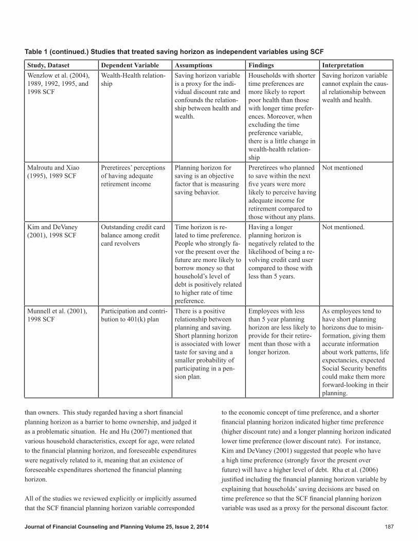
Study, Dataset Dependent Variable Assumptions Findings InterpretationWenzlow et al. (2004), 1989, 1992, 1995, and 1998 SCF

Wealth-Health relation-ship

Saving horizon variable is a proxy for the indi-vidual discount rate and confounds the relation-ship between health and wealth.

Households with shorter time preferences are more likely to report poor health than those with longer time prefer-ences. Moreover, when excluding the time preference variable, there is a little change in wealth-health relation-ship

Saving horizon variable cannot explain the caus-al relationship between wealth and health.

Malroutu and Xiao (1995), 1989 SCF

Preretirees’ perceptions of having adequate retirement income

Planning horizon for saving is an objective factor that is measuring saving behavior.

Preretirees who planned to save within the next five years were more likely to perceive having adequate income for retirement compared to those without any plans.

Not mentioned

Kim and DeVaney (2001), 1998 SCF

Outstanding credit card balance among credit card revolvers

Time horizon is re-lated to time preference. People who strongly fa-vor the present over the future are more likely to borrow money so that household’s level of debt is positively related to higher rate of time preference.

Having a longer planning horizon is negatively related to the likelihood of being a re-volving credit card user compared to those with less than 5 years.

Not mentioned.

Munnell et al. (2001), 1998 SCF

Participation and contri-bution to 401(k) plan

There is a positive relationship between planning and saving. Short planning horizon is associated with lower taste for saving and a smaller probability of participating in a pen-sion plan.

Employees with less than 5 year planning horizon are less likely to provide for their retire-ment than those with a longer horizon.

As employees tend to have short planning horizons due to misin-formation, giving them accurate information about work patterns, life expectancies, expected Social Security benefits could make them more forward-looking in their planning.

Table 1 (continued.) Studies that treated saving horizon as independent variables using SCF

to the economic concept of time preference, and a shorter financial planning horizon indicated higher time preference (higher discount rate) and a longer planning horizon indicated lower time preference (lower discount rate). For instance, Kim and DeVaney (2001) suggested that people who have a high time preference (strongly favor the present over future) will have a higher level of debt. Rha et al. (2006) justified including the financial planning horizon variable by explaining that households’ saving decisions are based on time preference so that the SCF financial planning horizon variable was used as a proxy for the personal discount factor.

than owners. This study regarded having a short financial planning horizon as a barrier to home ownership, and judged it as a problematic situation. He and Hu (2007) mentioned that various household characteristics, except for age, were related to the financial planning horizon, and foreseeable expenditures were negatively related to it, meaning that an existence of foreseeable expenditures shortened the financial planning horizon.

All of the studies we reviewed explicitly or implicitly assumed that the SCF financial planning horizon variable corresponded


Similarly, Wenzlow, Mullahy, Robert, and Wolfe (2004) stated “We include measures of time preference for saving in our analysis as a proxy for the individual discount rate…” and then describe the SCF financial planning horizon variable. However, they offered no justification as to why the SCF financial planning horizon variable was a good proxy for an individual’s discount rate. The Health and Retirement Study (HRS) dataset includes the same financial planning horizon question that is in the SCF, and a number of researchers have used the variable (Beri, 2012; Khwaja, Sloan, & Salm, 2006; Picone, Sloan, & Taylor, 2004; Smith, 1995). As with the studies using the SCF datasets, the authors assumed that the HRS financial planning horizon variable represented time preference.

Is it appropriate to consider the SCF and HRS financial planning horizon variables as true indicators of time preference? If financial planning horizon variables reflect only preferences, then many economists (e.g, Stigler & Becker, 1977) would start with the assumption that it was relatively stable over time for an individual, and did not change with circumstances. The studies we reviewed that used the SCF or the HRS financial planning horizon variables explicitly or implicitly assumed that the variables were good proxies for time preference. To test this assumption, further analyses are required such as examining the relationship between

household’s situational variables and the financial horizon variable. This motivated our study, investigating the effect of household situational variables on financial planning horizons.

MethodologyDataIn order to conduct statistical analysis for the financial planning horizon variable, we used Survey of Consumer Finances (SCF) datasets, based on a cross-sectional survey conducted every three years since 1983, and sponsored by the Federal Reserve Board. The purpose of this survey is to collect the U.S. household financial information such as income, assets, liabilities and investments as well as socio-demographic information. In order to have a large enough sample size for robust estimates of effects, we used a combination of the 1992 through 2007 datasets, for a total sample size of 25,889. We did not add in the 2010 SCF dataset for the analyses presented in this article as 2010 was very different from the other survey years because of the Great Recession. But our analysis using only the 2010 SCF dataset produced generally similar results, and would not change our conclusions. VariablesIn our study, the SCF financial planning horizon is the dependent variable. The original horizon variable (X3008) is

Study, Dataset

Independent Variables

Assumptions Findings Interpretation

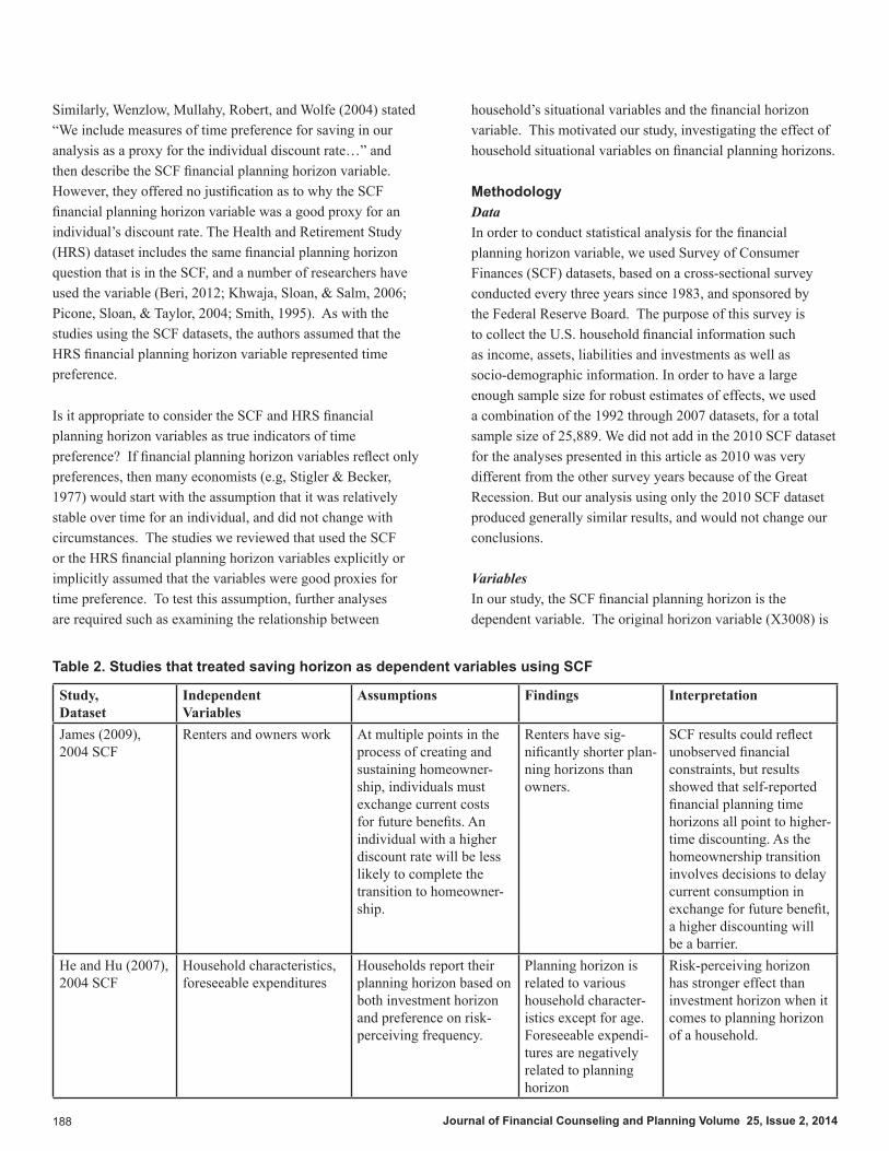
James (2009), 2004 SCF

Renters and owners work At multiple points in the process of creating and sustaining homeowner-ship, individuals must exchange current costs for future benefits. An individual with a higher discount rate will be less likely to complete the transition to homeowner-ship.

Renters have sig-nificantly shorter plan-ning horizons than owners.

SCF results could reflect unobserved financial constraints, but results showed that self-reported financial planning time horizons all point to higher-time discounting. As the homeownership transition involves decisions to delay current consumption in exchange for future benefit, a higher discounting will be a barrier.

He and Hu (2007), 2004 SCF

Household characteristics, foreseeable expenditures

Households report their planning horizon based on both investment horizon and preference on risk-perceiving frequency.

Planning horizon is related to various household character-istics except for age. Foreseeable expendi-tures are negatively related to planning horizon

Risk-perceiving horizon has stronger effect than investment horizon when it comes to planning horizon of a household.

Table 2. Studies that treated saving horizon as dependent variables using SCF


categorized into “next few months,” “next year,” “next few years,” “next 5-10 years,” and “longer than 10 years,” but we recode these categories to “0.3,” “1,” “3,” “7,” and “15.” As recoded numbers were arbitrary, we conducted a sensitivity analysis by using categories that were coded into “0.5,” “1,” “5,” “7.5” and “17.” The regression results were very similar to the results shown in Table 5. Independent variables in our study are household characteristic variables, which are proxies for household situational characteristics. The independent variables include survey year, age, marital status, education, race/ethnicity, presence of child, income, current income compared to normal income, home ownership, employment status, and health status. Among independent variables, marital status, race/ethnicity, education, current income compared to normal income, employment status and health status are measured as categorical variables. Survey year is included in our explanatory variables to see if there are any time trends. We also included age and age-squared to allow for nonlinear effects of age on financial planning horizon. Marital status is defined as four dummy variables: married, partner, single male, and single female. Respondent’s highest level of education is categorized into less than high school, high school, some college, and bachelor degree or higher. Race/ethnicity of the respondent includes White, Black, Hispanic, and other, a group that is largely Asian or Pacific Islander (Hanna & Lindamood, 2008). In order to allow for nonlinear effects, the natural log of income and of net worth was used in the regression. For values of zero or negative values, the log of 0.01 was used. Presence of child and home ownership were binary variables, coded as 1 if “yes” and 0 if “no.” Current income compared to normal income refers to whether current income is higher or lower compared to what would be expected in a normal year, containing three categories. If respondent’s current income is higher than their normal year, they are in the “income higher” category. On the other hand, if current income is lower compared to normal year, they are in the “income lower” category. If the income remains the same, then they are in the “normal” category. Employment status is composed of salary worker, self-employment, not working, and retirees. Health status differs depending on the respondent’s perception of health: excellent, good, fair, and poor health. For the multivariate analysis, the reference categories for categorical variables were 2004 survey year, married, no home ownership, less than high school education, White, no child, normal current income, salary worker, and excellent health categories.

AnalysisWe analyzed the distribution of the dependent variable of our

study, which is the recoded SCF horizon variable, and for descriptive purposes we found the mean level of the recoded horizon variable for each category of most of our independent variables. We weighted the descriptive analyses but did not weight the multivariate analysis (Lindamood, Hanna, & Bi, 2007). We ran an Ordinary Least Squares (OLS) regression analysis of the recoded financial planning horizon variable on socio-demographic variables and survey year. Since the original dependent variable is categorical, it is plausible that an ordered logistic regression (logit) is more appropriate than the OLS regression method. For this reason, we compared the results for Ordered Logistic and OLS regression, and found similar results. Most of the effects that were significant in the OLS regression were also significant in the logit. Therefore, we present the OLS regression results because interpretation of the magnitude of effects is easier. (The ordered logit regression results are available from the authors upon request.) Because of the imputed values for missing data, significance tests may be biased unless Repeated-Imputation Inference (RII) procedures are used (Lindamood et al., 2007; Montalto & Sung, 1996), we used RII procedures to obtain more valid estimates of variances and significance levels both for the means test in descriptive analyses and in the regression. Lindamood et al. (2007) noted that use of weights for multivariate analyses of SCF data is controversial, but unweighted analyses are better for hypothesis testing. Nielsen and Seay (2014) discussed the issue of considering complex sample structure in datasets such as the SCF. The SCF contains bootstrap weights to account for the complex structure, as well as population weights. Nielsen and Seay (2014) found only one article analyzing SCF datasets that used the bootstrap weights (Yao, Ying, & Micheas, 2013). The Yao et al. (2013) article did not mention the controversy about weighting SCF multivariate analyses. We present unweighted RII regression results, but none of our conclusions would change with a weighted analysis using bootstrap and population weights. (Results of a weighted analysis using bootstrap and population weights are available from the authors upon request.)

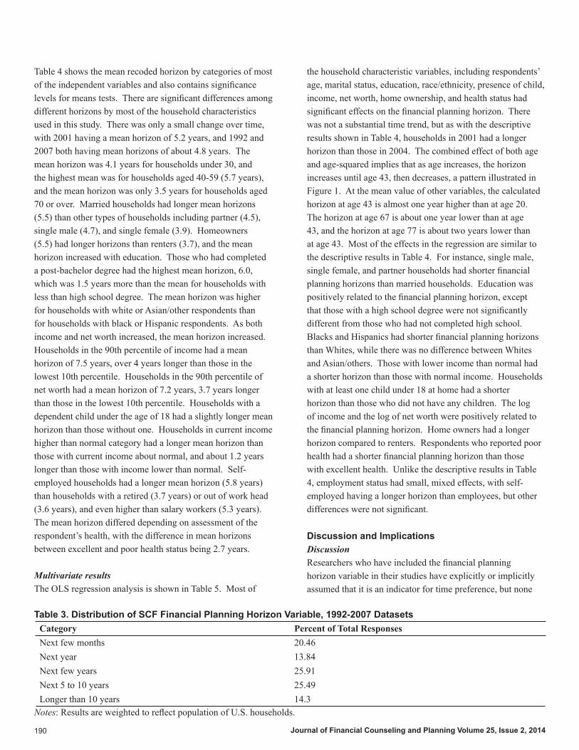
ResultsDescriptive ResultsTable 3 shows the distribution of the original SCF financial planning horizon variable from the 1992 to 2007 datasets. The midpoint and most typical response was “the next few years” with 26% of responses, although over 20% gave the “next few months” as a response. Only about 14% gave a horizon of “next year” or of “longer than 10 years.”


Table 4 shows the mean recoded horizon by categories of most of the independent variables and also contains significance levels for means tests. There are significant differences among different horizons by most of the household characteristics used in this study. There was only a small change over time, with 2001 having a mean horizon of 5.2 years, and 1992 and 2007 both having mean horizons of about 4.8 years. The mean horizon was 4.1 years for households under 30, and the highest mean was for households aged 40-59 (5.7 years), and the mean horizon was only 3.5 years for households aged 70 or over. Married households had longer mean horizons (5.5) than other types of households including partner (4.5), single male (4.7), and single female (3.9). Homeowners (5.5) had longer horizons than renters (3.7), and the mean horizon increased with education. Those who had completed a post-bachelor degree had the highest mean horizon, 6.0, which was 1.5 years more than the mean for households with less than high school degree. The mean horizon was higher for households with white or Asian/other respondents than for households with black or Hispanic respondents. As both income and net worth increased, the mean horizon increased. Households in the 90th percentile of income had a mean horizon of 7.5 years, over 4 years longer than those in the lowest 10th percentile. Households in the 90th percentile of net worth had a mean horizon of 7.2 years, 3.7 years longer than those in the lowest 10th percentile. Households with a dependent child under the age of 18 had a slightly longer mean horizon than those without one. Households in current income higher than normal category had a longer mean horizon than those with current income about normal, and about 1.2 years longer than those with income lower than normal. Self-employed households had a longer mean horizon (5.8 years) than households with a retired (3.7 years) or out of work head (3.6 years), and even higher than salary workers (5.3 years). The mean horizon differed depending on assessment of the respondent’s health, with the difference in mean horizons between excellent and poor health status being 2.7 years.

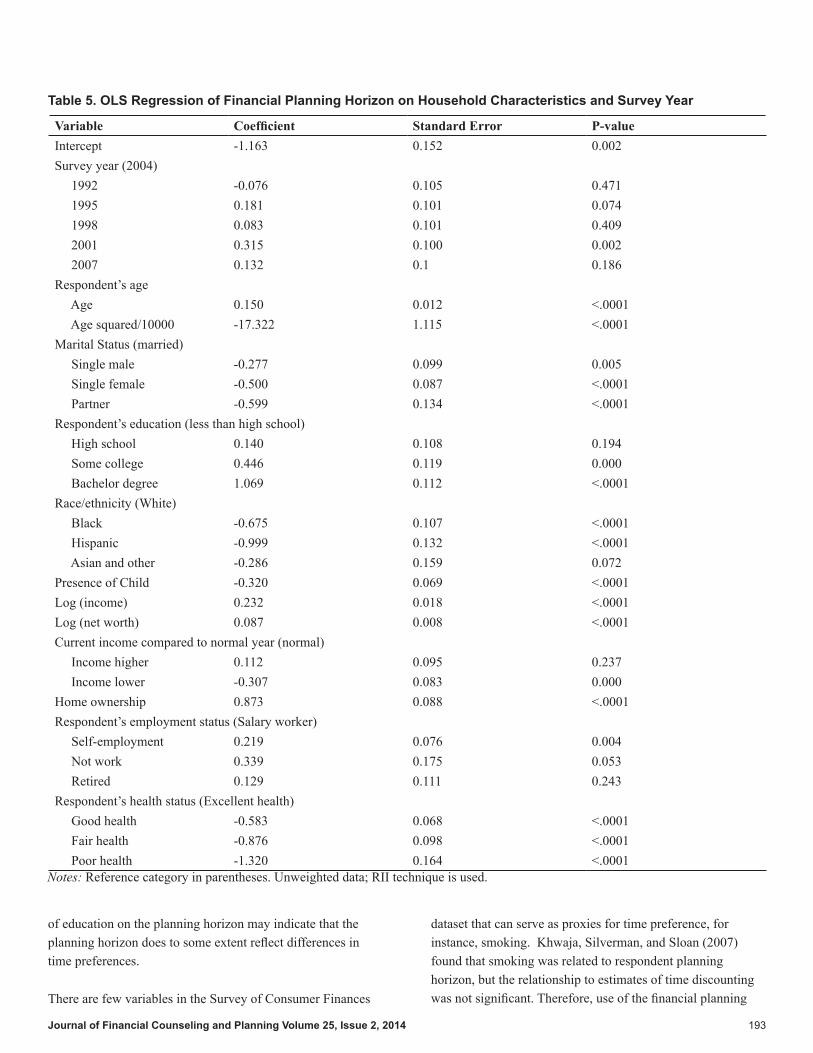
Multivariate results The OLS regression analysis is shown in Table 5. Most of

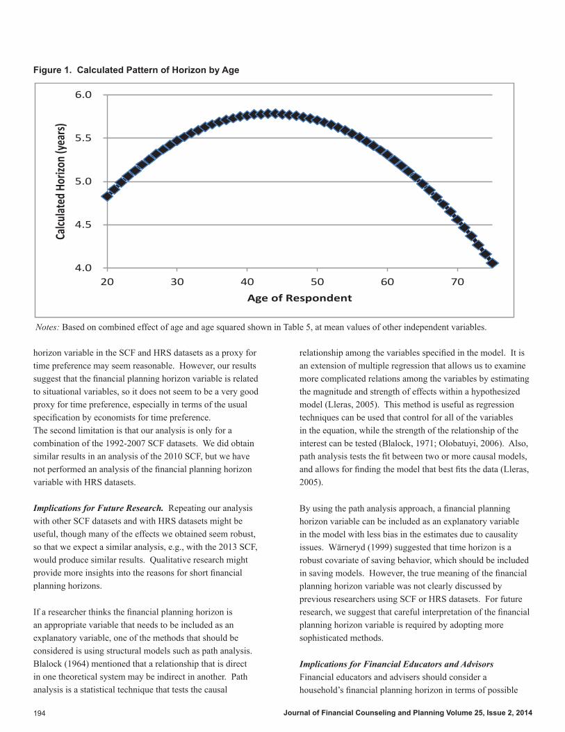
the household characteristic variables, including respondents’ age, marital status, education, race/ethnicity, presence of child, income, net worth, home ownership, and health status had significant effects on the financial planning horizon. There was not a substantial time trend, but as with the descriptive results shown in Table 4, households in 2001 had a longer horizon than those in 2004. The combined effect of both age and age-squared implies that as age increases, the horizon increases until age 43, then decreases, a pattern illustrated in Figure 1. At the mean value of other variables, the calculated horizon at age 43 is almost one year higher than at age 20. The horizon at age 67 is about one year lower than at age 43, and the horizon at age 77 is about two years lower than at age 43. Most of the effects in the regression are similar to the descriptive results in Table 4. For instance, single male, single female, and partner households had shorter financial planning horizons than married households. Education was positively related to the financial planning horizon, except that those with a high school degree were not significantly different from those who had not completed high school. Blacks and Hispanics had shorter financial planning horizons than Whites, while there was no difference between Whites and Asian/others. Those with lower income than normal had a shorter horizon than those with normal income. Households with at least one child under 18 at home had a shorter horizon than those who did not have any children. The log of income and the log of net worth were positively related to the financial planning horizon. Home owners had a longer horizon compared to renters. Respondents who reported poor health had a shorter financial planning horizon than those with excellent health. Unlike the descriptive results in Table 4, employment status had small, mixed effects, with self-employed having a longer horizon than employees, but other differences were not significant.

Discussion and ImplicationsDiscussionResearchers who have included the financial planning horizon variable in their studies have explicitly or implicitly assumed that it is an indicator for time preference, but none

Category Percent of Total ResponsesNext few months 20.46Next year 13.84Next few years 25.91Next 5 to 10 years 25.49Longer than 10 years 14.3

Table 3. Distribution of SCF Financial Planning Horizon Variable, 1992-2007 Datasets

Notes: Results are weighted to reflect population of U.S. households.


Category % Mean Sig. LevelAll households 100 4.91Survey year 1992 15.1 4.78 0.2816

1995 16.6 4.79 0.38451998 16.6 4.91 0.06292001 17.2 5.28 <0.00012004 17.5 4.832007 17.1 4.82 0.9180

Age of respondent <30 14.8 4.0930-39 20.4 5.26 <0.000140-49 21.8 5.69 <0.000150-59 16.3 5.60 <0.000160-69 12 4.80 <0.0001>69 14.7 3.46 <0.0001

Household type Married 51.6 5.54Partner 6.6 4.52 <0.0001Single male 14.3 4.69 <0.0001Single female 27.5 3.93 <0.0001

Home ownership No 33.2 3.70Yes 66.8 5.51 <0.0001

Education Less than high school 16.76 3.49High school 33.97 4.55 <0.0001Some college 18.01 4.93 <0.0001Bachelor degree 31.26 6.04 <0.0001

Racial/ethnic status White 75.7 5.23Black 12.8 3.77 <0.0001Hispanic 7.8 3.54 <0.0001Asian and other 3.7 5.02 <0.0001

Presence of dependent child<18

No 56.3 4.77Yes 43.7 5.08 <0.0001

Current Income <10,937 10.0 3.1710,937≤ income < 44,220 40.0 3.94 <0.000144,220≤income< 78,158 25.0 5.29 <0.000178,158≤income <12,7603 15.0 6.27 <0.0001127,603< 10.0 7.49 <0.0001

Net worth <43 10.0 3.4443≤net worth<92,110 40.0 4.05 <0.000192,110≤net worth< 285,498 25.0 5.23 <0.0001285,498≤net worth<727,039 15.0 6.12 <0.0001727,039< 10.0 7.15 <0.0001

Current income compared to normal year

Higher 9.2 5.58 <0.0001Lower 17.5 4.33 <0.0001Same 73.3 4.96

Table 4. Mean Financial Planning Horizon by Categories of Independent Variables


of them justified this assumption. In order to test whether this assumption is reasonable, we regress the SCF financial planning horizon variable on household characteristics. We hypothesize that if households’ characteristics were significantly related to the financial planning horizon, this indicates that the financial planning horizon variable is not a good proxy for time preference. Our regression analysis confirms that demographic variables of respondents are significantly related to the financial planning horizon, implying that the SCF variable is situational. While standard economic models regard time preference as exogenously given, our interpretation is that the financial planning horizon variable in the SCF and HRS datasets may reflect situational factors, and does not depend only on respondent’s time preference.

It is plausible to think that one’s financial planning horizon is situational rather than only an indicator of a permanent time preference. For instance, a person who is saving for a down payment to buy a home might have a short time horizon, but the same person after the home is purchased might then have a long time horizon, for instance, for retirement.

It is possible that some of the patterns indicate persistent differences over time, for instance, individuals who do not highly discount future benefits might be more likely to complete education beyond high school. It is also possible that those who discount the future less are likely to have higher incomes and net worth than those who do not. However, the patterns (see Figure 1) related to age and many of the other characteristics seem to suggest that the SCF horizon variable is not a time preference, and supports the conclusion that it is situational. For instance, having current income lower than normal is related to having a shorter horizon, and it does not seem plausible that this

would change one’s time preference. Is it plausible that the decrease in the financial planning horizon between 2001 and 2004, both in the means in Table 4 and in the regression in Table 5, indicates a change in time preference, or a change in situational considerations of the financial planning horizon? It is possible, as James (2009) suggested, that a more future-oriented time preference would make it more likely for some to become homeowners, but in our regression (Table 5), we are controlling for age, income, education, net worth, and presence of a child under 18. Perhaps part of the effect of homeownership on the financial planning horizon is that renters who would like to buy a home in the next few years might have a short financial planning horizon in terms of saving for a down payment. For similar reasons, it is plausible that those with a child under 18 have a shorter financial planning horizon because of the demands of having a young child.

Limitations and Implications for Future ResearchLimitations. Our analysis has two limitations. The first limitation is that the analysis does not demonstrate that the financial planning horizon variable is not related to time preference, only that it is related to many household situation variables such as age and presence of dependent children. It is difficult to judge whether some significant effects are related to situational differences, for instance, the shorter planning horizon of households with Black and with Hispanic respondents could be related to fundamental differences in time preference, but following the recommendation of Stigler and Becker (1977), we prefer to think of the racial/ethnic differences in planning horizon as reflecting past and expected situational variables that we do not control in our regression. The effect of education is more problematic for our conclusion, as it is plausible that more future-oriented individuals are more likely to finish degrees, so that the effects

Category % Mean Sig. LevelRespondent’s job status Self-employed 13.83 5.77 <0.0001

Salary worker 56.01 5.29No work 3.94 3.55 <0.0001Retired 21.81 3.72 <0.0001

Respondent’s health status Excellent 29.72 5.79Good 46.48 4.93 <0.0001Fair 18.15 3.97 <0.0001Poor 5.65 3.11 <0.0001

Table 4 (continued.) Mean Financial Planning Horizon by Categories of Independent Variables

Notes: Significance test is for mean difference from reference category for each variable. Bold is the reference category used in the mean test. Analyses weighted by population weight adjusted to reflect sample size; RII technique is used.


Variable Coefficient Standard Error P-valueIntercept -1.163 0.152 0.002Survey year (2004) 1992 -0.076 0.105 0.471 1995 0.181 0.101 0.074 1998 0.083 0.101 0.409 2001 0.315 0.100 0.002 2007 0.132 0.1 0.186Respondent’s age Age 0.150 0.012 <.0001 Age squared/10000 -17.322 1.115 <.0001Marital Status (married) Single male -0.277 0.099 0.005 Single female -0.500 0.087 <.0001 Partner -0.599 0.134 <.0001Respondent’s education (less than high school) High school 0.140 0.108 0.194 Some college 0.446 0.119 0.000 Bachelor degree 1.069 0.112 <.0001Race/ethnicity (White) Black -0.675 0.107 <.0001 Hispanic -0.999 0.132 <.0001 Asian and other -0.286 0.159 0.072Presence of Child -0.320 0.069 <.0001Log (income) 0.232 0.018 <.0001Log (net worth) 0.087 0.008 <.0001Current income compared to normal year (normal) Income higher 0.112 0.095 0.237 Income lower -0.307 0.083 0.000Home ownership 0.873 0.088 <.0001Respondent’s employment status (Salary worker) Self-employment 0.219 0.076 0.004 Not work 0.339 0.175 0.053 Retired 0.129 0.111 0.243Respondent’s health status (Excellent health) Good health -0.583 0.068 <.0001 Fair health -0.876 0.098 <.0001 Poor health -1.320 0.164 <.0001

Notes: Reference category in parentheses. Unweighted data; RII technique is used.

Table 5. OLS Regression of Financial Planning Horizon on Household Characteristics and Survey Year

dataset that can serve as proxies for time preference, for instance, smoking. Khwaja, Silverman, and Sloan (2007) found that smoking was related to respondent planning horizon, but the relationship to estimates of time discounting was not significant. Therefore, use of the financial planning

of education on the planning horizon may indicate that the planning horizon does to some extent reflect differences in time preferences.

There are few variables in the Survey of Consumer Finances


horizon variable in the SCF and HRS datasets as a proxy for time preference may seem reasonable. However, our results suggest that the financial planning horizon variable is related to situational variables, so it does not seem to be a very good proxy for time preference, especially in terms of the usual specification by economists for time preference.The second limitation is that our analysis is only for a combination of the 1992-2007 SCF datasets. We did obtain similar results in an analysis of the 2010 SCF, but we have not performed an analysis of the financial planning horizon variable with HRS datasets.

Implications for Future Research. Repeating our analysis with other SCF datasets and with HRS datasets might be useful, though many of the effects we obtained seem robust, so that we expect a similar analysis, e.g., with the 2013 SCF, would produce similar results. Qualitative research might provide more insights into the reasons for short financial planning horizons.

If a researcher thinks the financial planning horizon is an appropriate variable that needs to be included as an explanatory variable, one of the methods that should be considered is using structural models such as path analysis. Blalock (1964) mentioned that a relationship that is direct in one theoretical system may be indirect in another. Path analysis is a statistical technique that tests the causal

relationship among the variables specified in the model. It is an extension of multiple regression that allows us to examine more complicated relations among the variables by estimating the magnitude and strength of effects within a hypothesized model (Lleras, 2005). This method is useful as regression techniques can be used that control for all of the variables in the equation, while the strength of the relationship of the interest can be tested (Blalock, 1971; Olobatuyi, 2006). Also, path analysis tests the fit between two or more causal models, and allows for finding the model that best fits the data (Lleras, 2005).

By using the path analysis approach, a financial planning horizon variable can be included as an explanatory variable in the model with less bias in the estimates due to causality issues. Wärneryd (1999) suggested that time horizon is a robust covariate of saving behavior, which should be included in saving models. However, the true meaning of the financial planning horizon variable was not clearly discussed by previous researchers using SCF or HRS datasets. For future research, we suggest that careful interpretation of the financial planning horizon variable is required by adopting more sophisticated methods.

Implications for Financial Educators and AdvisorsFinancial educators and advisers should consider a household’s financial planning horizon in terms of possible

Figure 1. Calculated Pattern of Horizon by Age

Notes: Based on combined effect of age and age squared shown in Table 5, at mean values of other independent variables.

4.0

4.5

5.0

5.5

6.0

20 30 40 50 60 70

Calcu

lated

Hor

izon (

year

s)

Age of Respondent


situational factors, such as needing to save for a down payment for a home, or other particular goals. Having a short financial planning horizon when the most important goals are long-term might be an indication of having a high discounting of the future, but ascertaining the goals and needs of the household may be complex. For instance, a worker with a government defined benefit pension plan might feel that her long term financial goals are already taken care of, and might instead focus on short-term goals. Then focusing on a short-term goal does not necessarily mean that the worker highly discounts the future. Rather, household’s financial planning horizon is more related to situational factors, which may vary depending on household’s goals.

Practitioners should be careful in interpreting research that has used simple single equation estimations of effects of household attitudes that might be dependent on household situational factors. Based on our conclusion that the financial planning horizon variable may reflect situational factors, and not just time preference, future studies using this variable as an explanatory variable should use more complex models. Assuming that the financial planning horizon variable reflects time preference and ignoring possible structural patterns may make other independent variables appear to have non-significant effects. For instance, both Fisher and Montalto (2010) and Yuh and Hanna (2010) used the same dependent variable with the Survey of Consumer Finances, but Fisher and Montalto (2010) included the financial planning horizon as an independent variable, but Yuh and Hanna (2010) did not include it. Age and education variables were not significant in Fisher and Montalto’s (2010) study but were significant in Yuh and Hanna’s (2010) study. This may be due to the complex nature of the financial planning horizon variable.

ReferencesBecker, G. S., & Mulligan, C. B. (1997). The endogenous

determination of time preference. Quarterly Journal of Economics, 112(3), 729-758.

Beri, M. (2012). Essays on impact of risk preference on health and occupational choice. Wayne State University Dissertations. Paper 530. Retrieved from http://digitalcommons.wayne.edu/oa_dissertations/530

Bhargava, V., & Lown, J. M. (2006). Preparedness for financial emergencies: Evidence from the Survey of Consumer Finances. Journal of Financial Counseling and Planning, 17(2), 17-26.

Blalock, H. M. (1964). Causal inferences in nonexperimental research. Chapel Hill, NC: University of North Carolina Press.

Blalock, H. M., Jr. (1971). Causal models in the social sciences. Chicago, IL: Aldine Atherton.

DeVaney, S., & Hanna, S. D. (1991). The effect of children on savings. Proceedings of the Association for Financial Counseling and Planning Education, 207. Kansas City, MO.

Ersner-Hershfield, H., Garton, M. T., Ballard, K., Samanez-Larkin, G. R., & Knutson, B. (2009). Don’t stop thinking about tomorrow: Individual differences in future self-continuity account for saving. Judgment and Decision Making, 4, 280-286.

Fisher, P. J., & Montalto, C. P. (2010). Effect of saving motives and horizon on saving behaviors. Journal of Economic Psychology, 31(1), 92-105.

Frederick, S, Loewenstein, G., & Donoghue, T. O. (2002). Time discounting and time preference: A critical review. Journal of Economic Literature, 40(2), 351-401.

Freyland, F. (2004). Household composition and savings: An overview. Mannheim: Sonder forschungs bereich 504. WP No. 04-69.

Gomes, F., & Michaelides, A. (2005). Optimal life-cycle asset allocation: Understanding the empirical evidence. Journal of Finance, 60, 869-904.

Griesdorn, T. S. (2009). Risk tolerance and liquidity preferences of the self-employed. Proceedings of the Academy of Financial Services.

Hanna, S.D. & Kim, K. (2014). Time preference assumptions in normative analyses of household financial decisions. Applied Economics Letters, 21 (9), 609-612.

Hanna, S. D., & Lindamood, S. (2008). The decrease in stock ownership by minority households. Journal of Financial Counseling and Planning, 19, 46-58.

Hanna, S. D., & Rha, J. Y. (2000). The effect of household size changes on credit use: An expected utility approach. Consumer Interests Annual, 46, 121-126.

He, P., & Hu, X. (2007). Household investment - The horizon effect. Available at SSRN: http://ssrn.com/abstract=798431 or doi:10.2139/ssrn.798431.

Health and Retirement Study. (2014). Codebook. Variable NP041, http://hrsonline.isr.umich.edu/modules/meta/2012/core/codebook/h12p_ri.htm

James, R. N., III (2009). Tenant time preference as a barrier to homeownership. Applied Economics Letters, 16(10), 1073-1077.

Kim, H., & DeVaney, S. A. (2001). The determinants of outstanding balances among credit card revolvers. Journal of Financial Counseling and Planning, 12, 67-77.

Khwaja, A., Sloan, F., & Salm, M. (2006). Evidence on preferences and subjective beliefs of risk takers: The


case of smokers. International Journal of Industrial Organization, 24(4), 667-682.

Khwaja, A., Silverman, D., & Sloan, F. (2007). Time preference, time discounting, and smoking decisions. Journal of Health Economics, 26, 927-949.

Lleras, C. (2005). Path analysis. In Encyclopedia of Social Measurement (Vol. 3). St. Louis, MO: Elsevier Inc.

Lindamood, S., Hanna, S. D., & Bi, L. (2007). Using the Survey of Consumer Finances: Methodological considerations and issues. Journal of Consumer Affairs, 41(2), 195-214.

Malroutu, Y. L., & Xiao, J. J. (1995). Perceived adequacy of retirement income. Journal of Financial Counseling and Planning, 6, 17-23.

Montalto, C. P., & Sung, J. (1996). Multiple imputation in the 1992 Survey of Consumer Finances. Journal of Financial Counseling and Planning. 7, 133-146.

Munnell, A. H., Sunden, A., & Taylor, C. (2001). What determines 401(k) participation and contributions. Social Security Bulletin, 64(3), 64-76.

Nielsen, R. B. & Seay, M. C. (2014). Complex samples and regression-based inference: Considerations for consumer researchers. Journal of Consumer Affairs. doi: 10.1111/joca.12038.

Olobatuyi, M. E. (2006). A user’s guide to path analysis. Lanham, Maryland: University Press of America.

Picone, G., Sloan, F., & Taylor, J. D. (2004). Effects of risk and time preference and expected longevity on demand for medical tests. Journal of Risk and Uncertainty, 28(1), 39-53.

Rha, J. Y., Montalto, C. P., & Hanna, S. D. (2006). The effect of self-control mechanisms on household saving behavior. Journal of Financial Counseling and Planning, 17(2), 3-16.

Rutherford, L. G., & DeVaney, S. A. (2009). Utilizing the theory of planned behavior to understand convenience use of credit cards. Journal of Financial Counseling and Planning, 20(2), 48-63.

Samuelson, P. A. (1937). A note on measurement of utility. The Review of Economic Studies, 4(2), 155-161.

Smith, J. P. (1995). Racial and ethnic differences in wealth in the Health and Retirement Study. Journal of Human Resources, 30(0, Suppl.), S158-S183.

Stigler, G. J., & Becker, G. S. (1977). De gustibus non est disputandum. American Economic Review, 67(2), 76-90.

Wärneryd, K. E. (1999). The psychology of saving: A study on economic psychology. Northampton, Mass: E. Elgar.

Wenzlow, A. T., Mullahy, J., Robert, S. A., & Wolfe, B. L. (2004). An empirical investigation of the relationship

between wealth and health using the Survey of Consumer Finances. University of Wisconsin-Madison, Institute for Research on Poverty.

Yao, R. Ying, J., & Micheas, L. (2013). Determinants of defined contribution plan deferral. Family and Consumer Sciences Research Journal, 42(1), 55-76.

Yuh, Y., & Hanna, S. D. (2010). Which households think they save? Journal of Consumer Affairs, 44(1), 70-97.

About the AuthorsEunice O. Hong is a PhD candidate at The Ohio State University in the Human Sciences department studying Family Resource Management. She received an MS degree in Consumer Behavior and Family Economics from the University of Wisconsin-Madison, and a BS degree with dual majors in Economics and in Psychology from Ewha Womans University. She has presented papers at the American Council on Consumer Interests conference and the Academy of Financial Services conference.

Sherman D. Hanna is a Professor in the Department of Human Sciences at The Ohio State University. He is the Program Director for the undergraduate financial planning program registered with the CFP® Board. He is also Chair of the Consumer Sciences Graduate Studies Committee. He has published in Applied Economics Letters, Financial Services Review, Journal of Consumer Research, Journal of Consumer Affairs, Family and Consumer Sciences Research Journal, International Journal of Consumer Studies, Housing and Society, AAII Journal, Asia Pacific Advances in Consumer Research, International Journal of Human Ecology, Journal of Personal Finance, and Journal of Family and Economic Issues. He received a BS in economics from the Massachusetts Institute of Technology and a PhD in consumer economics from Cornell University.

financial planning horizon: a measure of time...

Documents