finding the homology of submanifolds with high...

Finding the Homology of Submanifoldswith High Confidence from Random

Samples

P. Niyogi�, S. Smale�, S. Weinberger�

September 13, 2004

Abstract

Recently there has been a lot of interest in geometrically moti-vated approaches to data analysis in high dimensional spaces. Weconsider the case where data is drawn from sampling a probabilitydistribution that has support on or near a submanifold of Euclideanspace. We show how to “learn” the homology of the submanifoldwith high confidence. We discuss an algorithm to do this and pro-vide learning-theoretic complexity bounds. Our bounds are obtainedin terms of a condition number that limits the curvature and nearnessto self-intersection of the submanifold. We are also able to treat thesituation where the data is “noisy” and lies near rather than on thesubmanifold in question.

1 Introduction

In recent years, there has been considerable interest in the possibility ofanalyzing and processing data in high dimensional spaces. Following theintuition that naturally occurring data may be generated by structured

�Departments of Computer Science, Statistics, University of Chicago.�Toyota Technological Institute, Chicago.�Department of Mathematics, University of Chicago.

1

systems with possibly much fewer degrees of freedom than the ambientdimension would suggest, various researchers (see [5, 2, 3, 6, 1] have con-sidered the case when the data lives on or close to a submanifold of theambient space. One hopes then to estimate geometrical and topologicalproperties of the submanifold from random points (“scattered data”) ly-ing on this unknown submanifold.In this paper, we consider the particular question of identifying the ho-mology of the submanifold from random samples. The homology of thesubmanifold (see [9] for definitions) are natural topological invariants thatprovide a good characterization of many aspects of it. For example, the di-mensions of the homology groups, the Betti numbers (�� ) have natu-ral interpretations. ��, the dimension of the zeroth homology group is thenumber of connected components of the submanifold. In data analysis sit-uations, the number of clusters of the data may sometimes be understoodin terms of the number of components of an underlying manifold (or othergeometric object). If the dimension of the submanifold is �, then one seesthat �� for all � � �. Thus the the largest non-trivial homology gives usthe dimension of the submanifold. If the submanifold is two-dimensional,then �� and �� are related to the number of connected components andnumber of holes respectively of the submanifold.We show that it is possible to identify the homology from random sam-ples and discuss an algorithm to do this. There are a few aspects of thedevelopments in this paper that are worth emphasizing. First, we providesample complexity estimates on the number of examples that are neededto identify the homology with high confidence. Our results are in the styleof learning theoretic treatments where unknown objects (typically func-tions in learning theory) are “learned” from random samples and confi-dence estimates are provided. Second, we treat the situation where datamight be drawn from a distribution that is concentrated around the mani-fold rather than precisely on it. Under specific models of noise, we showthat our algorithm can work even with noisy data. In all cases, estimatesare provided in terms of a condition number that limits the curvature andnearness to self-intersection of the submanifold.Our results may also be of interest to researchers in computational geome-try and topology who have considered the question of computing homol-ogy from simplicial complexes in the past (see [13, 7] for details and furtherreferences). Researchers in graphics, pattern recognition, solid modeling,molecular biology, finance, and other areas where large amounts of high

2

dimensional data are available may find some use for the topological per-spective on data analysis embodied in the algorithms and analyses of thispaper.

2 Preliminaries

Consider a compact Riemannian submanifold � of a Euclidean space��. Sample the manifold according to a uniform probability measureon it. Thus points �� are generated. This set of points �� will be the data set on the basis of which homology groupswill be calculated. In later sections, we will consider the case when thedata is drawn from a probability measure with support close to the mani-fold.Throughout our discussion, we will associate to � a condition number(�� ) where � defined as the largest number having the property: The opennormal bundle about � of radius is imbedded in �� for every � . Itsimage Tub� is a tubular neighborhood of � with its canonical projectionmap

�� Tub� ��Note that � encodes both local curvature considerations as well as globalones: If � is a union of several components � bounds their separation.For example, if � is a sphere, then � is equal to its radius. If � is anannulus, then � is the separation of its components. In Section 6 we re-late the condition number �

�to classical notions of curvature in differential

geometry via the second fundamental form.

3 An Outline of our Main Results

Ultimately we wish to compute the homology of the manifold � � ��

from the randomly sampled datapoints �� . We firstbegin by considering Euclidean balls (in the ambient space ��) of radius� and centers ��’s. Let us denote these balls as ��. We can now definethe open set � � �� given by

� � ��

3

Our first proposition states that if �� is �� dense in �, then� is a deformation retract of � .

Proposition 3.1 Let �� be any finite collection of points �� suchthat it is �

�dense in �, i.e., for every � � �, there exists an � � �� such that

� �� . Then for any �

�� , we have that � deformation retracts to

�. Therefore homology of � equals homology of�.

We prove this proposition in Section 4.In the case under consideration here, the points �� are sampled ini.i.d. fashion from the uniform probability distribution on �. By proba-bilistic considerations, we will then prove (in Section 5)

Proposition 3.2 Let �� be drawn by sampling � in i.i.d. fashion according tothe uniform probability measure on�. Then with probability greater than �� Æ,we have that �� is �

�-dense (� �

�) in � provided

��

Æ��

where ��

� and ��

��

. Here ��

� � denotes the

�-dimensional volume of the standard �-dimensional ball of radius �. Finally� � ��

��.

Putting these two propositions together, we see that we are able to providea finite sample estimate for how many times we need to sample� so thatwe are guaranteed with high confidence that the homology of the randomset � equals the homology of �. Thus our main theorem is

Theorem 3.1 Let � be a compact submanifold of �� with condition number � .Let �� be a set of � points drawn in i.i.d fashion according to theuniform probability measure on �. Let � � �

�. Let � � �� be a

correspondingly random open subset of ��. Then for all

� � ��

Æ��

the homology of � equals the homology of � with high confidence (probability� �� Æ).

4

3.1 Computing the Homology of �

One now needs to consider algorithms to compute the homology of � .Noting that the ��’s form a cover of � , one can construct the nerve ofthe cover. The nerve is an abstract simplicial complex constructed as fol-lows: One puts in a �-simplex for every � �-tuple of intersecting elementsof the cover. The Nerve Lemma (see [4]) applies in our case, as balls areconvex, to show that the homology of � is the same as the homology ofthis complex. The algorithm consists of the following components.

1. Given an �, and a set of points �� in ��, each �-simplexis given by a subset of the � points that have non-zero intersection.Thus we may define �� to be a simplicial complex (of dimension�). Each simplex � � �� is associated with a set of � � points(�� ) such that

��

An orientation for the simplex is chosen by picking an ordering andlet us denote the oriented simplex by �� .

2. A very crude upper bound on the size of �� (denoted by ��) isgiven by

��

��

�. However, it is clear that if two points �� and � are

more than � apart, they cannot be associated to a simplex. There-fore, there is a locality condition that the ��’s must obey whichresults in �� being much smaller than this crude number. The sim-plicial complex � � ��

� �� together with face relations.

3. A basic subroutine for computing the simplicial complex (steps 1 and2 above) involves the decision problem: for any set of � points, de-termine whether balls of radius � around each of these points havenon-empty intersection. This problem is related to the smallest ballproblem defined as follows: Given a set of � points, find the the ballwith smallest radius enclosing all these points. One can check that�� if and only if this smallest radius �. Fast algorithms

for the smallest ball problem exist. See [11] for theoretical discussionand “http://www2.inf.ethz.ch/personal/gaertner/miniball.html” fordownloadable algorithms from the web.

5

4. A �-chain is a function � � �� and can be written as a formalsum

� ��

��

By addition �-chains component wise, one gets the vector space of�-chains denoted by �� .

5. The boundary operator �� is a linear operator from�� to �� definedas follows. For each (oriented) simplex � � �� ,

��

��

��

where �� is a �� face of � (facing point ��) and the orientation of�� is given by �� . Now �� is defined on � chainsby additivity as

��

��

��

Thus, �� can be represented as a �� matrix where �� and �� respectively. The matrix is usually sparse in our set-ting.

6. This defines the chain complex

� � � ��

One can finally define the image and kernel of the boundary operatorgiven by

�� where �� and

�� Now �� is the vector space of �-boundaries and �� is thevector space of � cycles. Then the �th homology group is the quotientof �� over ��, i.e.,

��

6

The calculation of �� is seen to be an exercise in linear algebra giventhe matrix representation of the boundary operators. In our expo-sition here, we have been working over a field resulting in vectorspaces which are characterized purely by their ranks (the Betti num-bers). One approach to this is also via the combinatorial Laplacianas outlined in Friedman (1998). More generally, one can work over amodule and �� would then be an Abelian group.

4 The Deformation Retract Argument

In this section we prove Proposition 3.1 Consider the canonical map � �� given by (� is the restriction of �� to � )

��

��

Then we see that the fibers �� are given by

��

where �� is the normal subspace at � � � orthogonal to the tangent space �. Let us also define !"�� as

!"��

It is immediately clear that

!"��

Then the following simple proposition is true.

Proposition 4.1 !"�� is star shaped and therefore contracts to �.

PROOF:Consider arbitrary � � !"��. Then � � �� for some � � ��such that � � ��. Since � � ��, we immediately have � � ��.Since �� are both in ��, by convexity of Euclidean balls, we have thatthe line segment �� joining � to � is entirely contained in ��. At thesame time, �� is entirely contained in �� and it follows therefore that �� iscontained in !"��.

�

We next show that the inclusion of !"�� in �� is an equality provingthat �� contracts to �.

7

Proposition 4.2!"��

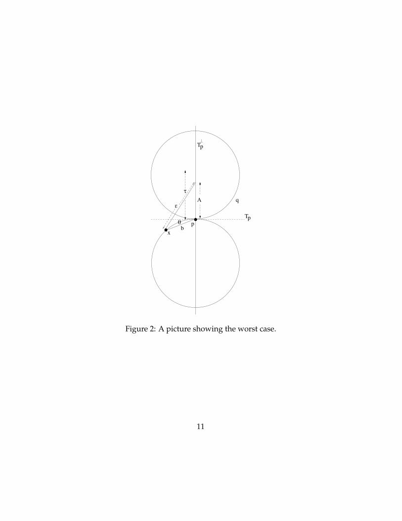
PROOF:We need to show that �� !"��. Consider an arbitrary � � ��#� �� where # � �� and # �� . For such � the picture offig. 1 can be drawn. Following lemma 4.1, we see that the distance of � to �is at most ��

�. Now by the fact that �� is �

�-dense, we have that there is some

point � � �� which is within ��

of �. The worst case picture of this is shownin fig 2. From lemma 4.2, we see that � � �� for this �. The propositionis proved.

�

These two propositions taken together show that � is a deformation re-tract of � . We see that�� . Further let $ �� "� � � � �� be givenby $ �� "� � "� �� "��. Then $ is continuous, $ �� and $ �� is the identity map.

Lemma 4.1 Consider any # �� Let � � ��#� �� . Then theEuclidean distance from � to � is less than ��

�.

PROOF:It suffices to consider # on the curve as shown in fig. 1. Followingthe symbols on the figure, we have

% � & �� &� ��

where & � � ��. Therefore, we have

% � � ��

From this we see that

�%

��

��

� � ��

�

It is easy to check that if � � , ��

�, i.e., % is monotonically decreasingwith �. Therefore the worst case situation is when & � � �� . Forthis value of �, we see that % � ��

�.

�

The following lemma ensures that there is an � � �� such that � � �� .

8

��

��

��

��

θ

ε

Ab

τq

pTp

Tp

Figure 1: A picture showing the worst case.

9

Lemma 4.2 Let �� be ��-dense in �. For any � � �, let � � ��. Then for� �

�� we have that � � �� for some � � �� .

PROOF:By the �� dense property, we know that there is an � � �� suchthat � � ��. Consider the picture in fig. 2. This represents the mostunfavorable position that such an � might have for the current context. Bythe same argument of lemma 4.1 we see that

% �� &� �� & ��

where & � � �� . Putting this value in, we have

% �

��

��

��

��

��

Simplifying, we see that % � ��

�if

��

��

��

�

�

��

�

Squaring both sides, we have

�

��

��

��

��

��

This simplifies to��

� �

�

�

Therefore, as long as � �

�� , we will have that � � �� for a suitable �.

�

5 Probability Bounds

Following our assumption, that the points �� are drawn at random, wenow provide a bound on how many examples need to be drawn so that theempirically constructed complex has the same homology as the manifold.We begin with a basic probability lemma.

10

��

��

��

q

pTp

Tp

bθ

εA

x

τ


11

Lemma 5.1 Let �%�� for ' � �� be a finite collection of measurable sets andlet ( be a probability measure on �

� �%� such that for all � � ' � �� we have(�%�� ). Let �� be a set of � i.i.d. draws according to (. Then if

� � �

)

��

�

Æ�

�

we are guaranteed that with probability � �� Æ, the following is true

�'� �� %� ��

PROOF:This follows from a simple application of the union bound. Let *�

be the event that ��%� is empty. The probability with which this happensis given by

��*� � �� (�%�� )��

Therefore, by the union bound, we have

��*� ��

� �

��*� � �� )��

It remains to show that for � � ��

��

Æ��, we have

�� )�� Æ

To see this, simply note that +�� for all � � �. Thisis seen by noting that +�� and + �� for all � � �. Putting� � ) in the above function, we have

�� )� � ��

and therefore it is easily seen that

�� )�� Æ

for the appropriate choice of �.�

12

Applying this to our setting, we consider a cover of the manifold � byballs of radius �

�. Let �,�� ' � �� be the centers of such balls that consti-

tute a minimal cover. Therefore, we can choose %� � ��,�� . Apply-

ing the above lemma, we immediately have an estimate on the number ofexamples we need to collect. This is given by

�

)

��

�

Æ�

�

where

) � ��

��%��

��

and � is the ��

covering number. These may be expressed entirely in termsof natural invariants of the manifold and we derive these quantities below.First, we note that the covering number may be bounded in terms of thepacking number, i.e., the maximum number of sets of the form -� � � � (at scale ) that may be packed into � without overlap. In particular,if �� is the �-covering number of � and . �� is the �-packing number,then the following simple lemma is true.

Lemma 5.2. �� . ��

PROOF:The fact that . �� follows from the definition. To see that�� . ��, begin by letting �� be a a realization of anoptimal �-packing so that - � . ��. We claim that �� form a �-cover. If not, there exists an � � � such that �� isempty for all '. In that case, one can add �� to the collection to increasethe packing number by � leading to a contradiction. Since �� is a valid �-cover, we have �� - � . ��.

�

Since � is the �� covering number, we see that � � . �� from lemma 5.2.Now we need to bound the packing number. To do so, we need the fol-lowing result.

Lemma 5.3 Let � � �. Now consider % � � ��. Then ��%� ��

� �� where �� is the �-dimensional ball centered at �, � �

�� . All volumes are �-dimensional volumes.

13

PROOF:Consider the tangent space at � given by � and let + be the pro-jection to �. Let �

� �� be the �-dimensional ball of radius centered at �lying in �. Let +� � �+�#� # � %� be the image of % under + . We willshow that �

� �� +�. Since + is a projection we have

��%� � ��+��

� ��

To see that �� +�, notice that + is an open map whose derivative is

nonsingular for all # � % (by Lemma 5.4). Therefore + is locally invertibleand there exists a ball �

� �� of radius ! such that +�� %. One

can keep increasing ! until it happens for the first time (say at ! � !�) that+��

� �� %. At this stage, there exists a point # in the closure of %such either (i) + is singular at # or (ii) # �� %. By Lemma 5.4, we see that (i)is impossible. Therefore, # �� % but # is in the closure of % implying that�# � �� . We see that !� � � �� where � is the angle between theline �#� (the line joining # to �) and the line �+�#�� (the line joining +�#� to �).By the curvature bound implied by � , we see that � � � and therefore!� � � �� . �

Lemma 5.4 Let � � �, let % � � ��, and let + be the projection to thetangent space at � ( �). Then for all � �

�, the derivative �+ is nonsingular at all

points # � %.

PROOF:Suppose �+ was singular for some # � %. That means that the tangentspace at # ( �) is oriented so that the vector with origin # and end point+�#� lies in �, in other words, � and � are at right angles to each other.Since # � ��, we have that � � # � � �

�. Putting propositions 6.2

and 6.3 together, we get that

��

��

where � is the angle between � and �. From this we see that � ��

leading to a contradiction.�

Using lemma 5.3, we see that a simple bound on the packing number isobtained. We obtain immediately that

. ��

��

14

Therefore, we have

� � . ��

��

��

��

where � � ��

�. Similarly, we have that

�

)� ��

��

6 Curvature and the Condition Number ��

In this section1, we examine the consequences of the condition number��

for the submanifold �. As we have mentioned before, � controls thecurvature of the manifold at every point. This fact has been exploited inour earlier proofs. For submanifolds, one may formally study curvaturethrough the second fundamental form (see e.g., [8]). Here we show for-mally that the norm of the second fundamental form is bounded by �

�.

Thus a large � corresponds to a well conditioned submanifold that haslow curvature.Proposition 6.1 states the bound on the norm of the second fundamentalform. Proposition 6.2 states a bound on the maximum angle between tan-gent spaces at different points in �. Proposition 6.3 states a bound onthe maximum difference between the geodesic distance and the ambientdistance for neighboring points in �.Let us begin by recalling the second fundamental form. Fix a point � ��. Following standard accounts (see, e.g. [8]), there exists a symmetricbilinear form � � � � � �� that maps any two vectors in the tangentspace (/� � � �) into a vector �/� �� in the normal space. Thus for anynormal vector (unit norm) 0 � �� , one can define the following

��/� �� 0� �/� �� /� 1��

where the inner product �� is the usual inner product in the tangentspace of the ambient manifold (in our case ��). Since � � � � � � ��is symmetric and bilinear, we see that 1� � � � � is a linear self-adjoint

1Thanks to Nat Smale for discussions leading to the writing of this section.

15

operator. The norm of the second fundamental form in direction 0 is nowgiven by

2� � ��

/� 1�/ �

/� / �

It is seen that 2� is the largest eigenvalue of 1�. Given this, we can provethe following proposition that characterizes the relation between the cur-vature through the second fundamental form and the condition numberof the submanifold.

Proposition 6.1 If� is a submanifold of �� with condition number ��, then the

norm of the second fundamental form is bounded by ��

in all directions. In otherwords, for all points � � � and for all (unit norm) 0 � �� , we have

2� � ��

/� 1�/ �

/� / ��

�

PROOF:We prove by contradiction. Suppose the proposition is false. Thenthere exists a point � � �, a tangent vector (unit norm) / � � and anormal vector (unit norm) 0 such that

0� �/� /� � ��

�

Consider a curve ��"� � � parametrized by arc length such that �� and !��

�� /. For convenience, we will place the origin at � so

that �� . With this (ambient) coordinate system, consider thepoint given by �0, i.e., the point a distance � from � in the direction 0. Byour hypothesis on the condition number of the submanifold, we see that� � � is the closest point on the manifold to the center of the � -ball givenby �0.

for all "� ��"�� 0� � � �

from which we get

�"� ��"�� "� � �� "�� 0 � � �

Consider the function 3�"� � ��"�� "� � �� "�� 0 �. Since �� ,we see that 3�� . Further, we have 3��"� � ��"�� !��"� � ��

16

!��"�� 0 �. Since �� and !�� 0 �� , we see that 3�� . Finally,3��"� � !��"�� !��"� � ��"�� "��"� � �� "��"�� 0 �. Since � isparameterized by arc length, we have !��"�� !��"� � � � and 3�� !�� 0 �.Noting that the tangent vector field ��

��is parallel (see proof of Proposi-

tion 6.2), we see that �� "��"�. Therefore, by assumption, we have

that 0� �/� /� �� 0� �

��

�"��

�"� �� 0� "��

�

�

Therefore, 3�� . By continuity, there exists a "� such that

3�"�� . But this leads to a contradiction since 3�"� � � for all ".�

Since the norm of the second fundamental form is bounded, we see thatthe manifold cannot curve too much locally. As a result, the angle betweentangent spaces at nearby points cannot be too large. Let � and # be twopoints in the submanifold � with associated tangent spaces � and �.Since � and � are affine subspaces of ��, one can compare them in theambient space in a standard way.Formally, one may transport the tangent spaces to the origin (according tothe standard connection defined in the ambient space ��) and then com-pare vectors in each of these tangent spaces with each other. Thus for any(unit norm) vectors / � � and � � �, we may define the angle � betweenthem by

�� /�� where �� is the usual inner product in ��, /�� are the vectors ob-tained by parallel transport (in ��) of / and � respectively to the origin.Hereafter, we will always take this construction as standard. We will dropthe prime notation and use /� � � to denote /�� in what follows.We can now state the following proposition.

Proposition 6.2 Let � be a submanifold of �� with condition number ��. Let

�� # � � be two points with geodesic distance given by �� #�. Let � be the theangle between the tangent spaces � and � defined by �� #�� /� � � . Then �� is greater than ��

�� #�.

PROOF:Consider two points �� # � � connected by a geodesic curve ��"� ��. Let ��"� be parametrized (proportional to arc length) so that �� ,and �� #.

17

Now let �� be a tangent vector (unit norm) and let ��"� be the paralleltransport of this vector along the curve ��"�. Thus we have �� ,�� . Clearly ��"�� "� �� for all " since � is parallel.Notice that

�� 4 �� 4 � (1)

where

4 �

� �

�

��

�"��" (2)

Combining 1 and 2, we see

�� 4 � � �� 4 (3)

where � is the angle between the vectors �� and ��. Since �� wasarbitrary, it is easy to check that �� .Now

��

�"� ��

��"�

where �� denotes the connection in Euclidean space. At the same time

� ��"� � � ��

��"��

where for any � � and � � � � (here � � is the tangent space of �� at ) wedenote by �� the projection of � onto � (here � is the tangent space to�at viewed as an affine space with origin ). But since ��"� is parallel, wehave that � ��

��"� � �. Therefore, ��

��"� is entirely in the space normal

to ��. But the component of �� "� in the normal direction is precisely

given by the second fundamental form. Hence, we have that

��

�"� �

��

�"� ��"��

where is a symmetric, bilinear form (the second fundamental form).Letting 0 be a unit norm vector in the direction ��

��, i.e., 0 � ��

��

��, we

see that

��" � 0�

��

�"�� 0� �

��

�"� ��"��

��

�"� 1��"� �

18

where 1� is a self adjoint linear operator. By Proposition 6.1, the norm of1� is bounded by �

�. Therefore, we have

��"� � ��

�"��1��

�"��1��

and

�4� � ��

�

��

�"� �

� �

�

��"� � �1��

� �

�

��"��" � �

�� #� (4)

Combining eq. 3 and eq. 4, we get

��

�� #�

�

We next show a relationship between the geodesic distance �� #� andthe ambient distance �� #�� for any two points � and # on the subman-ifold �.

Proposition 6.3 Let � be a submanifold of �� with condition number ��. Let

� and # be two points in � such that � � #�� . Then for all � � ��, the

geodesic distance �� #� is bounded by

�� #� � � � �

��

�

PROOF:Consider two points �� # � � and let ��"� be a geodesic curve join-ing them such that �� and ��!� � #. Let � be parametrized by arclength so that !��"� � � for all " and �� #� � !.Noting that the tangent vector field !� along the curve is parallel, we have"� � � !�� !�� and from proposition 6.1, we see that for all "

"� � � !�� !��

�

The chord length between � and # is given by ��!� � �� and we nowrelate this to the geodesic distance �� #�. Observe that

��!��

� �

�

!��"��"

19

Now

!��"� � !��

� �

�

"��

Thus !��"� � !�� /�"� where /�"� � �

�"��. We see that

/�"� ��

�

"�� "

�

Therefore,

��!��

�

!��"

� �

�

/�"��" � ! !��

�

/�"��" � !��

�

"

��"

Therefore we get

��!�� !� !�

�(5)

where � is the ambient distance between the points � and # while ! is thegeodesic distance between these same points. The inequality in eq. 5 is

satisfied only if ! � � � ��

�or ! � � �

��

�. Since ! � � when

� � �, we know that the second inequality does not apply. Therefore, fromthe first inequality, we have

! � � � �

��

�

�

7 Handling Noisy Data

In this section we show that if our data is noisy in the sense that it is drawnfrom a probability distribution that is concentrated around (rather thanon) the manifold, the homology of the manifold can still be computed fromnoisy data.

7.1 The Model of Noise

Consider a probability measure ( concentrated around the manifold. Weassume that ( satisfies the following two regularity conditions.

20

1. The support of ( (supp() is contained in the tubular neighborhoodof radius around �. Thus supp( � Tub��.

2. For every � ! , we have that

��$��

(� ��

where �� is a constant depending on ! and independent of �.

In what follows, we assume the data is drawn in i.i.d. fashion accordingto a . that satisfies the above properties.

7.2 Main Topological Lemma: Sufficient Conditions

We will proceed by constructing �-balls centered on our data points. Ifthese data are !-dense on the manifold, then the homology of the unionof these balls will equal that of the manifold � even if the data is drawnfrom a noisy distribution. In order to see that this might be the case at all,we provide a simple argument. This argument works with non-optimalchoices of � and ! and later sections will enter into the considerations ofchoosing better values for these parameters and therefore provide morenatural complexity estimates.Let �� be a set of � points in the tubular neighborhood ofradius around �. Let � be given by

� � ��

Proposition 7.1 If �� is -dense in � then � is a deformation retract of � for

all �� and � �

��

��

��

�.

PROOF:We show that for each � � �, it is the case that �� contractsto �. Consider a � � ��. Consider the line segment, ��, joining � to �.We claim that this line segment is entirely contained in ��. Clearly, if� � �� for some � � �� , this is immediate by the convexity ofballs in Euclidean space. So we only need to consider the situation where� � �� for some � �� . So let � � ��#� �� . Let

/ � ��

��

21

As long as / � �� for some � � �� , we see that the line segment�/� is contained in �� and therefore � contracts to �.Since we choose �, we are guaranteed that there is an � � �� . The worst case picture is shown in fig. 3. Following the symbols ofthe picture, as long as

� � % ��

we have that � contracts to �. Thus we need

�� %� � �� (6)

Expanding the squares, this reduces to

��

This is a quadratic in � and is satisfied for

� ��

��

��

�(7)

provided� � ��

This, in turn, is a quadratic in and it is easy to check that it is satisfied aslong as

��

��

�� (8)

Thus we see that for � � satisfying equations 7 and 8, we have that �contracts to �. �

We now need to compute the probability of drawing a random �� that isguaranteed to be -dense. The following proposition is true.

Proposition 7.2 Let-�� be the �-covering number of the manifold. Let ��

� be points on the manifold such that �� realize an �-cover of the mani-fold. Let �� be generated by i.i.d. draws according to a probability measure ( thatsatisfies the regularity properties described earlier. Then if if ��

��

��-��

Æ��,

with probability greater than �� Æ, �� will be -dense in �.

PROOF:Take %� � �� and apply Lemma 5.1. By the conclusion of thatlemma, we have that with high probability each of the %�’s is occupied byatleast one � � ��. Therefore it follows that for any � � �, there is atleast

22

��

��

��

��

pTp

T

qε

τ

r

p

A

x


23

one � � �� such that � � � . Thus with high probability �� is -denseon the manifold.

�

Putting these together, our main conclusion is

Theorem 7.1 Let -�� be the �-covering number of the submanifold � of��. Let �� be generated by i.i.d. draws according to a probability measure (that satisfies the regularity properties described earlier. Let � � �� .Then if if ��

�

��-��

Æ��, with probability greater than � � Æ,

� is a deformation retract of � as long as (1) ��

�� and (2) � ��

��

��

�

7.3 Main Topological Lemma – General Considerations

In general, we may demand points that are !-dense. Putting �-balls aroundthese points we construct � in the usual way. The condition number � andthe noise bound are additional parameters that are outside our controland determined externally. We now ask what is the feasible space �!� �� that will guarantee that � is homotopy equivalent to �?Following our usual logic, we see that the worst case situation is given byfig. 4. An arbitrary � � ��#� �� will contract to � if

��#� ��

This is the same as requiring

�� (9)

Additionally, we have the following equations that need to be satisfied(following fig. 4).

�� !� � �� (10)

!� � �� (11)

If one eliminates � and � from the above equations, one will get a singleinequality relating !� �� that describes for each �� the feasible set ofpossible choices of !� � that are sufficient to guarantee homotopy equiva-lence. Let us see how our earlier theorems follow from particular choicesof this general set of equations.

24

��

��

��

��

��

Tp

T

qε

τ

p

A

p r

ε v

β

x

τ−r


25

7.3.1 The Case when ! �

We have already examined the case when the points �� are chosen to be-dense in �. Putting in ! � in equations 9, 10, and 11, we see thefollowing:From eq. 10, we have (for ! � )

��

This simplifies to give � � .Putting � � and ! � in eq. 11, we get

� � � � ��

giving us � � �� .Finally, putting � � �� in inequality 9, we get

��

which is the same as inequality 6 whose solution was examined in theprevious section.

7.3.2 The Case when � �

We can recover our main theorem for the noise-free case by consideringthe case � �. We proceed to do this now.The fundamental inequality of 9 gives us (for � �)

��

This is the same as requiring

��

Using standard analysis for quadratic functions, we see that the followingcondition is required:

� � � �� (12)

We can eliminate � using equations 10 and 11. Thus, from eq. 10, we get� � ��

��and substituting in eq. 11, we get a quadratic equation in � whose

26

positive solution is given by � � ��

��

��

�� !��. This gives rise to

the following condition

� !�

�

�!�

�� !��

�� (13)

Inequality 13 gives the feasible region for ! and � for the homotopy equiv-alence of � and�. Let us consider the special case when ! � �

�— a choice

we made in Section 3 without any attention to optimality. Putting in thisvalue, after several simplifying steps, one obtains that

�� (14)

This is satisfied for all � �� or

� � ��

Remark 1 Note that in our original proof of our main noise free theo-rem (Theorem 3.1), the deformation retract argument of Section 3 passesthrough the construction of !"�� and shows contraction of �� by equat-ing it with !"��. This condition is stronger than we require. Here we seethat the condition ��#� �� is sufficient. This latter conditionis weaker and therefore gives us a slightly stronger version of Theorem 3.1in the sense that it holds for a larger range of �.Remark 2 If we assume that �� are beyond our control, the sample com-plexity depends entirely upon !. Therefore if we wish to proceed by draw-ing the fewest number of examples, then it is necessary to maximize ! sub-ject to the condition of eq. 13.Remark 3 The total complexity of finding the homology depends bothupon ! and � in a more complicated way. The size of �� depends entirelyupon ! and nothing else. However, the number of �-tuples to consider inthe simplicial complex depends both upon the size of �� as well as � because� determines how many balls will have non-empty intersections. We leavethis more nuanced complexity analysis for future consideration.

References

[1] A. Zomorodian and G. Carlsson. Computing persistent homology.20th ACM Symposium on Computational Geometry, Brooklyn, NY,June 9-11, 2004.

27

[2] J. B. Tenenbaum, V. De Silva, J. C. Langford. A global geomet-ric framework for nonlinear dimensionality reduction. Science 290(5500): 22 December 2000.

[3] M. Belkin and P. Niyogi. Semisupervised Learning on RiemannianManifolds. Machine Learning. Vol. 56. 2004.

[4] A. Bjorner. Topological Methods. in “Handbook of Combinatorics”,(Graham, Grotschel, Lovasz (ed.)), North Holland, Amsterdam, 1995.

[5] S. T. Roweis and L. K. Saul. Nonlinear dimensionality reduction bylocally linear embedding. Science 290: 2323-2326.2000.

[6] D. Donoho and C. Grimes. Hessian Eigenmaps: New Locally-LinearEmbedding Techniques for High-Dimensional Data. Preprint. Stan-ford University, Department of Statistics. 2003.

[7] T. K. Dey, H. Edelsbrunner and S. Guha. Computational topology.Advances in Discrete and Computational Geometry, 109-143, eds.: B.Chazelle, J. E. Goodman and R. Pollack, Contemporary Mathematics223, AMS, Providence, 1999.

[8] M. P. Do Carmo. Riemannian Geometry. Birkhauser. 1992.

[9] J. Munkres. Elements of Algebraic Topology. Perseus Publishing.1984.

[10] J. Friedman. Computing Betti Numbers via the Combinatorial Lapla-cian. Algorithmica. 21. 1998.

[11] K. Fischer, B. Gaertner, M. Kutz. Fast Smallest-Enclosing-Ball Compu-tation in High Dimensions. Proc. 11th Annual European Symposiumon Algorithms (ESA), 2003.

[12] Website for Smallest Enclosing Ball Algorithm.http://www2.inf.ethz.ch/personal/gaertner/miniball.html

[13] T. Kaczynski, K. Mischaikow, M. Mrozek. Computational Homology.Springer Verlag, NY. Vol. 157. 2004.

28

finding the homology of submanifolds with high...

Documents