finite element analysis for mechanical and aerospace design

CCOORRNNEELLLL U N I V E R S I T Y 1

MAE 4700 – FE Analysis for Mechanical & Aerospace Design N. Zabaras (02/13/2014)

Finite Element Analysis for Mechanical and Aerospace

Design

Prof. Nicholas Zabaras Materials Process Design and Control Laboratory

Sibley School of Mechanical and Aerospace Engineering 101 Rhodes Hall

Cornell University Ithaca, NY 14853-3801 [email protected]

http://mpdc.mae.cornell.edu

mailto:[email protected]

http://mpdc.mae.cornell.edu/



Weak Form • One of the key elements of the FE analysis is the

derivation of the weak (integral) form of the governing differential equations (strong form).

• This is the most critical step in the FEM.

• The process is common in all FEM procedures.

• Introduction of interpolation functions in the weak form will lead to the discretized FE equations.

• In this lecture, we work with 1D boundary value problems governed by ordinary differential eqs. (ODEs).



Strong form: Axial loading of an elastic bar

• Consider an elastic bar loaded as shown above. We introduce the following notation:

( ) intu x Displacement at po x

( ) ( / ) intx Stress force area at po xσ

( ) intdux Strain at po xdx

ε =

( ) intF x Internal force at po x

( ) sec intA x Cross tional area at po x

0x =

( ) ( / ) intb x Distributed load force length at po x

x L=




• We apply force balance on a differential element. • We will use the displacement as the main unknown. • Using , we can write: and the differential equation becomes:

0x = x L=

( )F x dx+( )F x ( )b x

( ) ( ) ( ) 02

( ) ( ) ( ) 0, 0,2

0

dxF x b x dx F x dx

F x dx F x dxb x take dxdx

dF bdx

− + + + + =

+ −+ + = →

+ =

,duF A E A EAdx

σ ε= = =

( )u x

( ) 0, 0d duEA b x Ldx dx

+ = < <

( ' )E Hooke s law constitutive equationσ ε= −




• To complete our problem definition, we need boundary conditions – in each end we need to prescribe either the displacement or the traction (force/area).

• For demonstration, let us take prescribed displacement at and prescribed traction at .

• So the complete strong form of our BVP is the following:

(0) (0)duE tdx

σ = = −

0t >


+ = < <

ux L= 0x =

( )u L u=

0x = x L=( )u L u=

t Sign convention The prescribed traction is taken as positive when is acting in the positive direction regardless on which face (left or right) is acting. The stress is positive in tension & negative in compression.



Heat conduction in one-dimension

• Consider heat conduction through a bar as shown above. We introduce the following notation:

( ) intT x Temperature at po x

( ) ( /( )) intq x Heat flux energy area time at po x×

( ) sec intA x Cross tional area at po x

0x =

( ) ( / ) intb x Heat source energy length at po x

x L=



Strong form: Heat conduction in a bar

• We apply energy balance on a differential element. • We will use the temperature as the main unknown. Substituting, leads to:

0x = x L=

( ) ( )q x dx A x dx+ +( ) ( )q x A x ( )b x

( )

in t

( ) ( ) ( ) ( ) ( ) 02

( ) ( ) ( ) ( ) ( ) 0, 0,2

heat flow in the CV heat flow out of the CVheat generated he CV

dxq x A x b x dx q x dx A x dx

q x dx A x dx q x A x dxb x take dxdx

d qAb

dx

− − + + + + =

+ + −− + = →

=

( ),dTq k Fourier law constitutive equationdx

= − −

( )T x

( ) , 0d dTkA b x Ldx dx

− = < <



Strong form: Heat conduction in a bar

• To complete our problem definition, we need boundary conditions – in each end we need to prescribe either the temperature or the heat flux.

• For demonstration, let us take prescribed temperature at and prescribed heat flux at .

• So the complete strong form of our BVP is the following:

(0) (0)dTq k qdx

= − = −

0q >

( ) 0, 0d dTkA b x Ldx dx

+ = < <

Tx L= 0x =

( )T L T=

0x = x L=( )T L T=

q Sign convention The prescribed flux is taken as positive if heat flows out of the bar. The heat flux q(0) as defined enters the system (i.e. is negative)



Weak form: Axial loading of an elastic bar

• To derive the weak form, multiply the ODE by an arbitrary weight function w(x) and integrate on the domain.

• Similarly for the natural BC. • These two equs. to be equivalent with those in the strong form, need to

be true for ALL w. We assume (we will come to this shortly) that w(L)=0.

(0) (0)duE tdx

σ = = −


+ = < <

( )u L u=

0x = x L=( )u L u=

t

0

( ) ( ) 0, ( ) 0L d duEA b w x dx w x in x L

dx dx + = ∀ < < ∫

0

(0) 0 0

x

duwA E t w on xdx

=

+ = ∀ =

σ

( )u L u=



Weak form: Axial loading of an elastic bar

• Integration by parts of the 1st equation gives:

0

( ) ( ) 0, ( ) 0L d duEA b w x dx w x in x L

dx dx + = ∀ < < ∫

0

(0) 0 0x

duwA E t w in x Ldx =

+ = ∀ ≤ ≤

( )u L u=

Compute u(x):

0 0 0| 0, ( ) 0 , ( ) 0

L Lx Lx

du du dwEA w EA dx bwdx w x in x L with w Ldx dx dx

== − + = ∀ < < =∫ ∫

• Using the weak form of the traction BC and that , we can simplify:

00 0

| , ( ) 0 , ( ) 0L L

xdu dwEA dx wAt bwdx w x in x L with w Ldx dx == + ∀ < < =∫ ∫

( ) 0w L =



Weak problem statement • Find u(x) among the smooth functions with such that ( )u L u=

• The integration by parts leads to a symmetric form in u and w – this leads to a symmetric stiffness after finite element discretization is introduced.

• The weak statement is EQUIVALENT to the strong form. In other words, not only if u(x) satisfies the strong form the above is true, but also if u(x) satisfies the weak form then it is also the solution of the strong form of our problem.

• Smoothness in u and w is needed for the integrals in the weak form to exist (we need H1 functions u and w that have 1st derivative that is squared integrable)!

00 0

| , ( ) 0 , ( ) 0L L




1st derivative squared integrable functions • What smoothness conditions on u and w we need for the

integrals in the weak form to exist?

• In the first integral, we have product of 1st order derivatives of u and w. We need to have functions for which this integral exists.

• Thinking for a moment (because of the symmetry in u and w) that u=w, we want trial u and weight w functions that are 1st derivative square integrable, i.e. functions such that:

00 0

| , ( ) 0 , ( ) 0L L


2

0

, 0L dvEA dx EA

dx < ∞ > ∫

1( ) ( ),v x H I∈[0, ]I L=



Continuous functions with piecewise continuous derivatives

• A function with V-continuity, can have discontinuity (kinks) in its slope.

00 0

|L L

xdu dwEA dx wAt bwdxdx dx == +∫ ∫

• Find such that the following holds:

, ( ) ,u V with u L u∈ =

, ( ) 0,w V with w L∀ ∈ =

: [0, ], ' se cV v v is continuous on I L v is piecewi ontinuous and bounded on I= =

• Let us select as a function space to define the weak form the following:

• Can you verify that this type of functions will work for our weak form?

• A function in V is piecewise continuously differentiable, i.e. its first derivative is continuous except at selected points.



C-1 continuity • Consider functions (C-1 continuity) with discontinuities

(jumps) and discontinuities in slope (kinks) • Such functions that are not infinite have 1st order derivatives

that are integrable (you can integrate delta functions!)

• However, note that in our weak form we have a product of the 2 derivatives:

• If both u and w are in C-1 and have a discontinuity at the same point a of magnitudes α and β, respectively, then the 1st integral in the eq. above takes the form:

• So the C-1 functions are not good candidates for our weight and trial functions.

0

L du dwEA dxdx dx∫

2

0

( )L

x a dxαβδ −∫ This integral does not exist!



C0 functions • Let us define the C0-continuity functions as follows:

• These functions in general are not appropriate as weight

and trial functions in our weak form.

• Indeed, consider the following function:

• It is C0 continuous for all λ>0, however an H1 function (e.g. 1st derivative square integrable) only for λ>1/2. Verify this by computing analytically.

1 1( )2 2

( )1 1 1( ) ( )2 2 2

x x

u x

x x x

− ≤

=

− − >

λ

λ λ

0 ( ) : [0, ]C I v v is a continuous function defined on I L= =

21

0

du dxdx

∫

C0 continuous but not H1 function

0 0.1 0.2 0.3 0.4 0.5 0.6 0.7 0.8 0.9 1-0.4

-0.35

-0.3

-0.25

-0.2

-0.15

-0.1

-0.05

0

0.05

x

u(x)

C0 function,Lambda=0.45



Continuous functions with piecewise continuous derivatives versus H1

• We will see in an upcoming lecture, that in finite element analysis we consider piecewise polynomial (linear, quadratic, etc.) functions on subdivisions (triangulations) of a bounded domain on elements.

• Our selection of finite element approximation space , is satisfied in this case by selecting

• This is the case since will be shown to be continuous between the boundaries of adjacent elements and that its first derivative exists and is piecewise continuous so that

[0, ]I L=

1( )hV H I⊂0 ( )hV C I⊂

1( )v H I∈

0 ( )v C I∈



Weak formulation in H1

• When producing weak (variational) formulations of boundary value problems, it is (from mathematical point of view) natural and very useful to work with function spaces that are slighlty larger (i.e. spaces that contain more functions) than the spaces of continuous functions with piecewise continuous derivatives introduced earlier.

• It is also useful to endow V with scalar products and corresponding norms related to the actual boundary value problem.

00 0

|L L


• Find such that the following holds:

, ( ) ,u V with u L u∈ =

, ( ) 0,w V with w L∀ ∈ =

: [0, ], ' se cV v v is continuous on I L v is piecewi ontinuous and bounded on I= =



The weak form in H1 • We modify the weak problem statement as follows:

• The space H1, is the space of 1st derivative square integrable functions.

• H1 is the largest space we can write the above weak form and it naturally arises from the specific BVP. We will also see that the basic error estimate for the FE is in the H1 norm.

2

int0

1( ) , 02

L

Internalstrainenergy

duW u EA dx EAdx

= < ∞ > ∫

int ( )W uwe will later introduce as the energy norm.

00 0

|L L


Find such that the following holds:

1, ( ) ,u H with u L u∈ =1, ( ) 0,w H with w L∀ ∈ =



Square integrable functions L2(I) • Consider in 1D the interval I=(0,L). We define the space of

square integrable functons on I as:

• The space L2(I) is a Hilbert space with the (L2-) scalar (inner) product:

and corresponding (L2-) norm: • By Cauchy’s inequality:

• For this class, think of as a piecewise continuous function, possibly unbounded, such that: .

• As an example, for if

22 ( ) :

I

L I v v is defined on I and v dx

= < ∞

∫

2 ( )( , )L II

v w vwdx= ∫2

1/2

2 1/2( )|| || ( , )L I

I

v v dx v v

= = ∫

2 2 2( ) ( ) ( )| ( , ) | || || || ||L I L I L Iv w v w≤

2 ( )v L I∈2

I

v dx < ∞∫

2(0,1), ( ) ( )x I v x x L I−∈ = = ∈β 1/ 2.<β



First derivative square integrable functions H1(I) • We formally introduce the space H1(I), I=(0,L) as follows:

• The space H1(I) consists of the functions defined on I which together with their 1st derivatives are square integrable.

• This space is equipped with the following inner (scalar) product:

• The corresponding norm is:

• When v(0)=0 and/or v(L)=0, in literature, we often denote the corresponding space as

12( ) : ' ( )dvH I v v and v belong to L I

dx = ≡

1 ( )( , ) ( ' ')

H II

v w vw v w dx= +∫( )1

1/2

2 2( )

|| || ( ')H I

I

v v v dx

= + ∫

01 1( ) ( ) : ( ) 0H I v H I v L= ∈ =



Recall smoothness conditions for beams • Recall that beam shape functions were C1 continuous –

both displacements and slopes were continuous (4th other ODEs).

22 2

2( )2 2

y

e e

ee e e ee

d uE I E IU dx dxdx

κΩ Ω

= =∫ ∫

22

2 2yd udV dq EI

dx dx dx

= − =



Weak form Strong form • We will here show that if u satisfies the weak form, it is also

a solution of the strong form. Let u:

• Integrate backwards the first term as follows:

000

| , ( ) 0 , ( ) 0L

L


0 000

| | , ( ) 0 , ( ) 0L

LLx

du d duEA w EA wdx wAt bwdx w x in x L with w Ldx dx dx =

− = + ∀ < < = ⇒ ∫ ∫

00( ) | 0, ( ) 0 , ( ) 0

L

xd duEA b wdx wA t w x in x L with w Ldx dx

σ =

+ + + = ∀ < < = ∫

• Since w(x) is arbitrary, select with a smooth function with e.g.

( ) d duw x EA bdx dx

ψ = + ( ) 0xψ > (0) ( ) 0Lψ ψ= = ( )x L xψ = −



Weak form Strong form

• With this selection of w, the Eq. above becomes:

• With , the above can be true only if:

• This proves that if u is a solution of the weak form, it also satisfies the ODE strong form. It remains to show that it satisfies the natural BC.

00( ) | , ( ) 0 , ( ) 0

L


σ = + + + ∀ < < =

∫

2

0( ) 0

L d dux EA b dxdx dx

ψ + = ∫

( ) 0xψ >

0, 0d duEA b x Ldx dx

+ = < <



Weak form Strong form

• Returning to the above equation, we have:

• Since w is arbitrary, select it such that w(0)=1, w(L)=0, then

• In conclusion, if u is a solution of the weak form, it also satisfies the complete strong form of our BVP.

00( ) | 0, ( ) 0 , ( ) 0

L


σ =

+ + + = ∀ < < = ∫

0( ) | 0, ( ) ( ) 0xwA t w x with w Lσ =+ = ∀ =

0t at xσ = − =



Strong form: Axial loading of an elastic bar • Let us generalize the earlier examined problem by allowing

arbitrary part of the boundary with prescribed displacement and the remaining part with prescribed traction:

• The nornal vector n is introduced to allow arbitrary application of the traction BC (recall ). If n=1 (right boundary), then . If a positive force is applied at the left boundary (n=-1), then .

tdun E n t ondx

σ = = Γ


+ = < <

uu u on= Γ

uΓtΓ

0t >

tt onσ = Γ

tt onσ = − Γ

0u t

u t

Γ ∩Γ =Γ ∪Γ = Γ



Weak form: Axial loading of an elastic bar • Multiplying the ODE with w and integrating by

parts gives:

• We require that this holds for , where and for all with is the space of 1st derivative square integrable functions.

• As before, the weak form is symmetric in u and w (first derivatives for both u and w). This will lead to a symmetric stiffness matrix.

| 0, ( ) 0 , 0 udu du dwEA wn EA dx bwdx w x in x L with w ondx dx dxΓ

Ω Ω

− + = ∀ < < = Γ ⇒∫ ∫

| , ( ) 0 , 0t u

du dwEA dx Awt bwdx w x in x L with w ondx dx Γ

Ω Ω

= + ∀ < < = Γ∫ ∫1( )u x H∈

uu u on= Γ 1( )w x H∈ 0 .uw on= Γ 1H



Summary of weak forms for the two problems • Axial deformation problem: Find ,

• Heat conduction problem: Find ,

10 ( ) , 0 uU w x H w in= ∈ = Γ

( )u x U∈ 1 ( ) , uU u x H u u in= ∈ = Γ

0| , ( ) ,q

du dwAk dx Awq bwdx w x Udx dx Γ

Ω Ω

= − + ∀ ∈∫ ∫1

0 ( ) , 0 uU w x H w in= ∈ = Γ

( )u x U∈ 1 ( ) , uU u x H u u in= ∈ = Γ

0| , ( ) ,t

du dwEA dx Awt bwdx w x Udx dx Γ

Ω Ω

= + ∀ ∈∫ ∫



Minimum potential energy • We used earlier the principle of mimimum potential

energy to derive the FEM eqs. • How is this method related to the weak form? Let

us revisit the elastic bar problem.

0x = x L=( )u L u=

t

int

2

( ),

( )( )

1( ) , min ( ) ( ) |2 t

ext

u xKinematically admissibledisplacements W Wsatisfy kinematicdisplacement boundary

conditions u L u

duFind u x U such that AE dx ubdx uAtdx Γ

Ω Ω

=

∈ − +

∫ ∫



Minimum potential energy

• We will show that the minimizer of the potential energy satisfies the weak form (and thus the strong form).

• P(u(x)) is a functional – takes a function as an input and returns a scalar! We need to use calculus of variations for its mimimization.

• A variation of the function u is denoted by δu(x) ≡ζw(x) where w(x) is an arbitrary function, and 0<ζ<1 is a very small positive number.

int

( )

2

( ) , min ,

1 ( ) ( ) |2 t

ext

u x

W W

Find u x U such that where

duP AE dx ubdx uAtdx Γ

Ω Ω

∈ Ρ

= − +

∫ ∫



Variation of a functional • The corresponding change in the functional is called

the variation in the functional and denoted by δW , which is defined by

• From the principle of minimum potential energy, it is clear that the function u(x) +ζ w(x) must still be in U. To meet this condition, w(x) must be smooth and vanish on the essential boundaries, i.e.

• So w(x) vanishes at the parts of the boundary with essential boundary conditions!

=P(u(x)+ w(x))-P(u(x))=P(u(x)+ u(x))-P(u(x))Pδ ζ δ

0w U∈



Variation of the internal energy • Let us evaluate the variation of the first term in

• Dropping the higher order terms in ζ, leads to:

int .W

2 2

int

2 2 22

1 12 2

1 122 2

du dw duW AE dx AE dxdx dx dx

du du dw dw duAE dx AE dxdx dx dx dx dx

δ ς

ς ς

Ω Ω

Ω Ω

= + −

= + + −

∫ ∫

∫ ∫

intdu dwW AE dxdx dx

δ ςΩ

= ∫



Variation of the external work • Let us evaluate the variation of the 2nd term,

• Combining the last 2 terms, the variation of the potential energy is given as:

• Minimization of the potential energy requires: for any

.extW( ) ( ) | | |

t t textW u w bdx u w At ubdx uAt wbdx wtΓ Γ ΓΩ Ω Ω

= + + + − − = +∫ ∫ ∫δ ς ς ς ς

|t

du dwP AE dx wbdx wAtdx dx Γ

Ω Ω

= − −∫ ∫δ ς ς ς

0,Pδ =, . . :u w i e for anyδ ς ς=

|t

du dwAE dx wbdx wAtdx dx Γ

Ω Ω

= +∫ ∫



Variational principle

• This is identical with our weak form. So minimization of the potential energy leads to the same solution as the weak problem, thus

• Note that now we understand why in the weak form we considered w to vanish on the boundary with essential conditions: and the miminization is wrt functions u(x) that satisfy the essential BCs, thus

|t

du dwAE dx wbdx wAtdx dx Γ

Ω Ω

= +∫ ∫

rStrong p oblem Weak problem Variational problem⇔ ⇔

( )u w xδ ς=

| ( ) | 0 ( ) | 0u u u

u w x w xδ ςΓ Γ Γ= = ⇒ =



Principle of virtual work • The minimization of P,

• This can also be written as ( ) :

• This is simplified as:

0,Pδ =

| 0t

du dwP AE dx wbdx wAtdx dx Γ

Ω Ω

= − − =∫ ∫δ ς ς ς

| 0t

dV

du d uP E Adx ubdx uAtdx dxσ δε

δδ δ δ ΓΩ Ω

= − − =∫ ∫

int

| 0t

extW W

P dV ubdx uAt ΓΩ Ω

= − + =

∫ ∫

δ δ

δ σδε δ δ

u wδ ζ≡



Principle of virtual work

• The internal work done by the actual stresses on the arbitrary strains induced by the arbitrary

displacements is equal to the external work done by the body forces and applied tractions on the arbitrary displacement field .

• This statement is of course the same as the weak form but presented in ` mechanics’ language.

int

| 0t

extW W

P dV ubdx uAt ΓΩ Ω

= − + =

∫ ∫

δ δ

δ σδε δ δ

d udxδδε ≡

0u Uδ ∈b t

uδ



Limitations of the variational principle • There are many problems to which the variational

principle is not applicable. For example, variational principles cannot be developed for the advection-diffusion equation.

• Variational principles can only be developed for systems that are self-adjoint.

• The weak form for the advection-diffusion equation is not symmetric, and it is not a self-adjoint system.



Example problem 1 • Derive the weak form for the following BVP:

• We multiply by w and integrate from 1 to 3, for every w, w(3)=0.

• Integration by parts of the 1st term gives:

(10 ) 2 0,1 3, (1) 0.1, (3) 0.001d du dux x udx dx dx

+ = < < = =

3

1

(10 ) 2 0, , (3) 0d du x wdx w wdx dx

+ = ∀ = ∫

3 331

1 1

10 | 10 2 0, , (3) 0xx

du du dww dx xwdx w wdx dx dx

== − + = ∀ = ⇒∫ ∫

3 3

1 100.1

10 (3) (3) 10 (1) (1) 10 2 0, , (3) 0du du du dww w dx xwdx w wdx dx dx dx

− − + = ∀ = ⇒∫ ∫3 3

1 1

10 (1) 2 , , (3) 0du dw dx w xwdx w wdx dx

= − + ∀ =∫ ∫



Example problem 2

• For the problem discussed earlier, consider a trial (candidate) solution of the form and a weight function of the same form, . Obtain a solution to the weak form shown above. – Check if the equilibrium equation in the strong form is

satisfied? – Check if the natural boundary condition is satisfied?

• Since w(3)=0,

3 3

1 1


= − + ∀ =∫ ∫

0 1( ) ( 3)u x x= + −α α

0 1( ) ( 3)w x x= + −β β

0 1 1 1( ) ( 3) ( ) ( 3) dww x x w x x anddx

β β β β= + − ⇒ = − =



Example problem 2

• Substitution in the weak form gives:

• So the solution is:

• Is the strong form satisfied?

• Is the natural BC satisfied?

3 3

1 1


= − + ∀ =∫ ∫

0 1 1 1 1( ) ( 3), , ( ) ( 3),du dwu x x w x xdx dx

α α α β β= + − = = − =

3 3

1 1 1 1 11 1

10 2 2 ( 3) ,dx x x dx= + − ∀ ⇒∫ ∫α β β β β1 1 1 1 1

2020 2 ,3

= − ∀ ⇒α β β β β

1 120 720 23 30

= − ⇒ = −α α

7( ) 0.001 ( 3) ( (3) 0.001)30

u x x here we used u= − − =

7(10 ) 2 (10 ) 2 2 0,30

d du dx x x not satisfieddx dx dx

+ = − + = ≠

7(1) 0.1,30

du not satisfieddx

= − ≠



Example problem 3 • Find the weak form of the following BVP:

• Multiplying by w with w(0)=w(1)=0 and integration from 0 to 1 gives:

22

2 2 0, 0 1, (0) 1, (1) 2, , tand uk u x x u u k cons tsdx

− + = < < = = −λ λ

1 22

20

2 0, , (0) (1) 0d uk u x wdx w w wdx

− + = ∀ = = ⇒

∫ λ

1 1 12

0 0 0

(1) (1) (0) (0) 2 0, , (0) (1) 0du du du dwk w k w k dx uwdx x wdx w w wdx dx dx dx

− − − + = ∀ = = ⇒∫ ∫ ∫λ

1 1 12

0 0 0

2 , , (0) (1) 0du dwk dx uwdx x wdx w w wdx dx

+ = ∀ = =∫ ∫ ∫λ



Example problem 4 • Consider a bar subjected to linear

body force b(x)= Cx . The bar has a constant cross-sectional area A and

Young’s modulus E. Assume quadratic trial solution and weight functions:

u(x)=α1+α2x+α3 x2

w(x)= β1+β2x+β3 x2

• For what value of αi is u(x) kinematically admissible?

• Using the weak form, set up the equations for αi and solve.

• Solve the problem using two 2-node elements of equal size like the elements we used in the lecture on truss structures (direct method).

Approximate the external load at node 2 by integrating the body force from x=L/4 to x=3L/4; Likewise compute the external at node 3 by integrating the body force from x=3L/4 to x=L.



Example problem 4 • On • The constraint on the weight

functions is then:

• The weak for this problem is the following:

1: (0) 0 0u uΓ = ⇒ =α

1(0) 0 0w = ⇒ =β

22 3 2 3

22 3 2 3

( ) , 2

( ) , 2

duu x x x xdxdww x x x xdx

= + = +

= + = +

α α α α

β β β β

0 0

| 0t

L Ldu dwAE dx wbdx wAtdx dx Γ− − = ⇒∫ ∫

( )( ) ( )22 3 2 3 2 3

0 0

2 2L L

AE x x dx C x x xdx+ + = + ⇒∫ ∫α α β β β β

( ) ( )2 2 32 2 2 3 3 2 3 3 2 3

0 0

2 2 4L LAE x x x dx x x dx

Cβ α β α β α β α β β+ + + = + ⇒∫ ∫



Example problem 4

( )

( )

22 2 2 3 3 2 3 3

0

2 32 3 2 3

0

2 2 4

,

L

L

AE x x x dxC

x x dx

β α β α β α β α

β β β β

+ + +

= + ∀ ⇒

∫

∫

( ) ( )2 2 32 2 2 3 3 2 3 3 2 3 2 3

0 0

(2 2 ) 4 ,L LAE x x dx x x dx

C+ + + = + ∀ ⇒∫ ∫β α β α β α β α β β β β

2 3 3 4

2 2 2 3 3 2 3 3 2 3 2 3(2 2 ) 4 ,2 3 3 4

AE L L L LLC

+ + + = + ∀ ⇒

β α β α β α β α β β β β

( )3 3 4

2 22 2 3 3 2 3 2 34 0 ,

3 3 4AE L AE L LL L LC C

+ − + + − = ∀ ⇒

β α α β α α β β

2 3 2

2 22 3 4

3 3

73 12

443 4

AEL AEL L CLC C AE

CLAEL AEL LAEC C

= ⇒ = ⇒

−

α αα α

227( )

12 4CL CLu x x xAE AE

= −



Example problem 4

3f2f

3 /4 2

2/4

2

33 /4

4

732

L

LL

L

CLf Cxdx

CLf Cxdx

= =

= =

∫

∫

(1) (2)

1 1 01 1 1 12 2 2, , 1 2 11 1 1 1

0 1 1

AE AE AEK K KL L L

− − − = = = − − − − −

Our final system of assembled equations is the following:

12

2

23

1 1 0 02 1 2 1

40 1 1

732

rAE CLuL

uCL

− − − = ⇒ −

2

22

3

2 12 41 1 7

32

CLuAEuL CL

− = ⇒ −

3

23

3

15641132

CLu AEu CL

AE

=

32

1 22 2 15 15( ) ( )

64 32AE AE CLr u CLL L AE

= − = − = −



Discretized weak form with finite elements • Consider the following BVP:

• We multiply the equation −u’’ = f by an arbitrary function

• Integrate over (0, 1) which gives: −(u’’, w) = (f, w) [ We use the following notation: ]

• We now integrate the left-hand side by parts using the fact that w(0) = w(1) = 0 to get:

−(u’’, w) = −u’(1)w(1) + u’(0)w(0) + (u’, w’) = (u’, w’) • We conclude that:

• We are next going to look for approximate solutions using piece-wise

linear C0 (continuous) functions.

−u’’(x) = f(x), 0 < x < 1

u(0) = u(1) = 0

1

0

( , )f g fgdx≡ ∫

( ', ') ( , ),u w f w w V= ∀ ∈

w V∈

1 1

0 0: du dwor equivalently dx fwdx w V

dx dx= ∀ ∈∫ ∫



Finite element discretization: Piecewise linear functions • Construct a finite-dimensional subspace Vh ⊂ V as follows:

• Define intervals Ij = (xj−1, xj) of length hj = xj − xj−1, j = 1, 2, . . . , (M + 1) and set h = maxj hj.

• Let Vh be the set of functions v such that: – v is linear on each subinterval Ij – v is continuous on [0, 1] and – v(0) = v(1) = 0. • The quantity h = maxj hj is a measure of how fine the

partition is.



Piecewise linear basis functions Nj(x), j = 1, 2, . . .,M

• A function has the representation:

where for i,j=1,…,M

Nj (xi) = δij

• The space Vh is a linear space of dimension M with basis Ni, i=1,..,M

1( )

( ) ( ) ( ), 0 1M

i ii Nodal values

of v x

v x v x N x x=

= ≤ ≤∑

N1

N2

N3

This is not much different from a Fourier expansion – the difference is that we use piecewise linear functions instead of sin and cos functions

These are global basis functions each one defined for each global node

10( ) (0,1)iN x H∈

hv V∈



Linear system of equations: Stiffness and load • We approximate the solution as with uh(xj) the nodal values of uh(x). • Recall our weak formulation: • It now takes the form:

• The space Vh is spanned by M functions Ni, thus the weak

form takes the form:

• We now left with substituting in this equation:

1( ) ( ) ( ), 0 1

M

h h j jj

u x u x N x x=

= ≤ ≤∑

' ': ( , ) ( , ), hh h h h hFind u u w f w w V= ∀ ∈

' ': ( , ) ( , ), 1,2,...,h h i iFind u u N f N i M= =

1( ) ( ) ( ).

M

h h j jj

u x u x N x=

=∑' '

1( ) : ( , ) ( ) ( , ) , 1,2,...,

iij j

M

h j j i h j ij FK d

Find u x N N u x f N i M=

= =∑

( ', ') ( , ),u w f w w V= ∀ ∈



Properties of the stiffness matrix

• K is symmetric: Kij = Kji, • K is sparse (i.e. only a few elements of K are

nonzero)

• K is positive definite: Indeed for we obtain:

' '

1: ( , ) ( ) ( , ) , 1,2,...,

iij j

M

h j i h j ij FK d

Find u N N u x f N i M=

= =∑

1

1

' '2 2

1 1

1 1 1 1( , ) , 1,2,...,j j

j j

x x

j j x xj j j j

N N dx dx j Mh h h h

+

− + +

= + = + =∫ ∫

1

' ' ' '1 1 2

1 1( , ) ( , ) , 2,...,j

j

x

j j j j xj j

N N N N dx j Mh h−

− −= = − = − =∫' '( , ) 0, | | 1i jN N i j= − >

' ' ' '

1 1 1 1 1 1. ( , ) ( , ) ( , ) 0

M M M M M M

i ij j i i j j i i j ji j i j i j

K K N N N N= = = = = =

= = = = ≥∑∑ ∑∑ ∑ ∑

η

η η η η η η η η η η

. 0, 0.K only for= =η η η

' ' ' '( , ) ( , ), , 1,2,...,j i i jN N N N i j M= =

jN1jN −

Mη∀ ∈

1 1' '

0 0

: , ( )ij i j i iwhere K N N dx F f x N dx= =∫ ∫



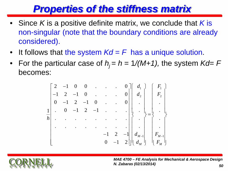
Properties of the stiffness matrix • Since K is a positive definite matrix, we conclude that K is

non-singular (note that the boundary conditions are already considered).

• It follows that the system Kd = F has a unique solution. • For the particular case of hj = h = 1/(M+1), the system Kd= F

becomes:

1 1

2 2

1 1

2 1 0 0 . . . 01 2 1 0 . . . 0

. .0 1 2 1 0 . . 0

. .. 0 1 2 1 . . .1

. .. . . . . . . .

. .. . . . . . . .1 2 1

0 1 2M M

M M

d Fd F

h

d Fd F

− −

− − − − − − − = − − −



Final solution • Let us assume that

the solution obtained with 3 nodes (excluding the boundary nodes with u=0) is the following:

• The piece-wise linear representation of the FE solution is shown here.

1 1 2 2 2 3

1 2 3

( ) ( ) ( ) ( ) ( ) ( ) ( )0.9 ( ) 0.7 ( ) 0.2 ( )

h h h hu x u x N x u x N x u x N xN x N x N x

= + + =

+ +

( ) ( )h i iu x N x

( )hu x

10.9 ( )N x 20.7 ( )N x

30.2 ( )N x

finite element analysis for mechanical and aerospace design

Documents