First Approximation for Uniform Lower and

Upper Bounded Facility Location Problem

avoiding violation in Lower Bounds

June 28, 2021

Sapna Grover1, Neelima Gupta2 and Rajni Dabas3

1. Department of Computer Science, University of Delhi, India.sgrover@cs.du.ac.in, sapna.grover5@gmail.com

2. Department of Computer Science, University of Delhi, India.ngupta@cs.du.ac.in

3. Department of Computer Science, University of Delhi, India.rajni@cs.du.ac.in

AbstractWith growing emphasis on e-commerce marketplace platforms where

we have a central platform mediating between the seller and the buyer, itbecomes important to keep a check on the availability and profitability ofthe central store. A store serving too less clients can be non-profitable anda store getting too many orders can lead to bad service to the customerswhich can be detrimental for the business. In this paper, we study thefacility location problem(FL) with upper and lower bounds on the numberof clients an open facility serves. Constant factor approximations areknown for the restricted variants of the problem with only the upperbounds or only the lower bounds. The only work that deals with boundson both the sides violates both the bounds [8]. In this paper, we presentthe first (constant factor) approximation for the problem violating theupper bound by a factor of (5/2) without violating the lower boundswhen both the lower and the upper bounds are uniform. We first givea tri-criteria (constant factor) approximation violating both the upperand the lower bounds and then get rid of violation in lower bounds bytransforming the problem instance to an instance of capacitated facilitylocation problem.

1 Introduction

Facility location problem (FL) is a well motivated and extensively studied prob-lem. Given a set of facilities with facility opening costs and a set of clients with

1

arX

iv:2

106.

1137

2v3

[cs

.DS]

25

Jun

2021

a metric specifying the connection costs between facilities and clients, the goalis to select a subset of facilities such that the total cost of opening the selectedfacilities and connecting clients to the opened facilities is minimized.

With growing emphasis on e-commerce marketplace platforms where we havea central platform mediating between the seller and the buyer, it becomes im-portant to keep a check on the availability and profitability of the central store.A store serving too less clients can be non-profitable and a store getting toomany orders can lead to bad service to the customers. This scenario leads towhat we call as the lower- and upper- bounded facility location (LBUBFL)problem. There are several other applications requiring both the lower as wellas the upper bound on the number of clients assigned to the selected facilities.In a real world transportation problem presented by Lim et al. [17], there area set of carriers and a set of customers who wish to ship a certain number ofcargoes through these carriers. There is a transportation cost associated to shipa cargo through a particular carrier. The goal of the company is to ship cargoesin these carriers such that the total transportation cost is minimized. There isa natural upper bound on the number of cargoes a carrier can carry imposed bythe capacity of the carrier. In addition, the shipping companies are required toengage their carriers with a “minimum quantity commitment” when shippingcargoes to United States. Another scenario in which the problem can be usefulis in the applications requiring balancing of load on the facilities along withmaintaining capacity constraints.

In this paper, we study the facility location problem with lower and upperbounds. We are given a set C of clients and a set F of facilities with lower boundsLi and upper bounds Ui on the minimum and the maximum number of clientsa facility i can serve, respectively. Setting up a facility at location i incurs costfi(called the facility opening cost) and servicing a client j by a facility i incurscost c(i, j) (called the service cost). We assume that the costs are metric, i.e.,they satisfy the triangle inequality. Our goal is to open a subset F ′ ⊆ F andcompute an assignment function σ : C → F ′ (where σ(j) denotes the facility thatserves j in the solution) such that Li ≤ |σ−1(i)| ≤ Ui ∀i ∈ F ′ and, the total costof setting up the facilities and servicing the clients is minimised. The problemis known to be NP-Hard. We present the first (constant factor) approximationfor the problem with uniform lower and uniform upper bounds, i.e., Li = L andUi = U ∀i ∈ F without violating the lower bounds, as stated in Theorem 1.2.

Definition 1.1. A tri-criteria (α, β, γ)- approximation for LBUBFL problemis a solution S = (F ′, σ) satisfying αL ≤ |σ−1(i)| ≤ βU ∀i ∈ F ′, α ≤ 1, β ≥ 1,with cost no more than γOPT , where OPT denotes the cost of an optimalsolution of the problem.

Theorem 1.2. A (1, 5/2, O(1))- approximation can be obtained for LBUBFLin polynomial time.

Constant factor approximations are known for the problem with upper boundsonly (popularly known as Capacitated Facility Location (CFL)) with [20, 6, 9]and without [14, 7, 1, 19, 18, 22, 5, 3] violating the capacities using local search

2

/ LP rounding techniques. Constant factor approximations are also known forthe problem with lower bounds only with [13, 10, 12] and without [21, 2, 16]violating the lower bounds. The only work that deals with the bounds on boththe sides is due to Friggstad et al. [8], which deals with the problem with non-uniform lower bounds and uniform upper bounds. They gave a constant factorapproximation for the problem using LP-rounding, violating both the upper andthe lower bound by a constant factor. The technique cannot be used to get ridof the violation in the lower bounds even if they are uniform as the authorsshow an unbounded integrality gap for the problem. Thus, our result is an im-provement over them when the lower bounds are uniform in the sense that theyviolate both the bounds whereas we do not violate the lower bounds.

1.1 Related Work

For capacitated facility location with uniform capacities, Shmoys et al. [20] gavethe first constant factor(7) algorithm with a capacity blow-up of 7/2 using LProunding techniques. An O(1/ε2) factor approximation, with (2+ε) violation incapacities, follows as a special case of CkFLP by Byrka et al. [6]. Grover et al. [9]reduced the capacity violation to (1+ ε). For non-uniform capacities, Levi et al.[15] gave a 5-factor approximation algorithm using LP-rounding for a restrictedversion of the problem in which the facility opening costs are uniform. Later,An et al. [3] gave the first LP-based constant factor approximation algorithmwithout violating the capacities, by strengthening the natural LP.

The local search technique has been particularly useful to deal with capac-ities. Korupolu et al. [14] gave the first constant factor (8 + ε) approximationfor uniform capacities, which was further improved by Chudak and Williamson[7] to (6 + ε). The factor was subsequently reduced to 3 by Aggarwal et al. [1],which is also the best known result for the problem. For non-uniform capacities,Pal et al. [19] gave the first constant factor (8.53 + ε) approximation algorithmwhich was subsequently improved to (7.88 + ε) by Mahdian and Pal [18] and to(5.83 + ε) by Zhang et al. [22] with the current best being (5 + ε) due to Bansalet al. [5].

Lower-Bounded Facility Location (LBFL) problem was introduced by Kargerand Minkoff [13] and Guha et al. [10] independently in 2000. Both of them gavea bi-criteria algorithm, that is a constant-factor approximation with constantfactor violation in lower bounds. Zoya Svitkina [21] presented the first trueconstant factor(448) approximation for the problem with uniform lower boundsby reducing the problem to CFL. This was later improved to 82.6 by Ahmadianand Swamy [2] using reduction to a special case of CFL called CapacitatedDiscounted Facility Location. Later Shi Li [16] gave the first true constant(4000) factor approximation for the problem with non uniform lower bounds.Li obtained the result by reducing the problem to CFL via two intermediateproblems called, LBFL-P(Lower bounded facility location with penalties) andTCSD(Transportation with configurable supplies and demands). Han et al. [12]gave a bi-criteria solution for the problem as a particular case of lower boundedk-FL problem when the lower bounds are non-uniform.

3

Another variant of LBFL, called Lower bounded k-Median problem(LBkM)was considered by Guo et al. [11] and Arutyunova and Schmidt [4] with uniformlower bounds, where they gave constant factor approximations for the problemsby reducing them to CFL and LBFL respectively. For Lower bounded k-FacilityLocation problem LBkFL problem with non-uniform lower bounds, Han et al.[12] presented a bi-criteria algorithm giving α factor violaton in lower boundsand 1+α

1−αρ-approximation where ρ is the approximation ratio for kFL problemand α is a constant. They also extend these results to LBkM and lower boundedknapsack median problem.

Friggstad et al. [8] is the only work that deals with the problem with boundson both the sides. The paper considers non-uniform lower bounds and uniformupper bounds. They gave a constant factor approximation, using LP roundingtechniques, violating both the lower and the upper bounds.

1.2 High Level Idea

Let I be an input instance of the LBUBFL problem. We first present a tri-criteria solution (> 1/2, 3/2, O(1)) violating both the lower as well as the upperbound and then get rid of the violation in the lower bound by reducing theproblem instance I to an instance Icap of CFL via a series of reductions (I →I1 → I2 → Icap). As we will see that maintaining α > 1/2 is crucial in gettingrid of the violation in the lower bound and hence the tri-criteria solution ofFriggstad et. al. [8] cannot be used here as α < 1/2 in their work. Also,when the lower bounds are uniform, our approach is comparatively simpler andstraightforward. Let CostI(S) denotes the cost of a solution S to an instanceI. We work in the following steps:

1. We first compute a tri-criteria solution (> 1/2, 3/2, O(1)) - approximationSt = (F t, σt) to I via clustering and filtering techniques. Thus, α > 1/2and β = 3/2.

2. We transform the instance I into another instance I1 of LBUBFL bymoving the clients assigned to a facility i in the tri-criteria solution St

to i. Let O denote the optimal solution of I. To construct a solution ofI1, a client j is assigned to a facility i if it was assigned to i in O. Theconnection cost is bounded by the sum of the cost j pays in St and in O.Thus, CostI1(O1) ≤ CostI(St) +CostI(O) where O1 denotes the optimalsolution of I1.

3. The instance I1 is transformed into another instance I2 of LBFL, ignoringthe upper bounds. The facility set is reduced to F t and the facilitiesin F t are assumed to be available free of cost. If a client j is assigned,in O1, to a facility i not in F t then it is assigned to the facility i′ ∈F t nearest to i (assume that the distances are distinct) and we openi′. The connection cost is bounded by twice the cost j pays in O1 by asimple triangle inequality. Let O2 denote the optimal solution of I2. Then,CostI2(O2) ≤ 2CostI1(O1).

4

4. Finally, we create an instance Icap of CFL from I2. The key idea in thereduction is: let ni be the number of clients assigned to a facility i in F t.If i violates the lower bound, we create a demand of L − ni at i in theCFL instance otherwise we create a supply of ni−L at i. The solution ofthe CFL instance then guides us to increase the assignments at some ofthe violating facilities until it gets L clients or decides to shut them. Theprocess results in an increased violation in the capacities by plus 1.

Let Ocap be an optimal solution of Icap. We show that CostIcap(Ocap) ≤

(1 + 2δ)CostI2(O2) for an appropriately chosen constant δ.

5. We obtain an (5 + ε)-approximate solution AScap for Icap by using thealgorithm of Bansal et al. [5] for CFL. Thus, CostIcap(AScap) ≤ (5 +ε)CostIcap(Ocap).

6. From AScap, we obtain an approximate solution AS1 to I1 such that theupper bounds are violated by a factor of (β + 1) with no violation in

lower bounds and CostI1(S1) ≤ 2(α+1)(2α−1)CostIcap

(AScap). Facility trees are

constructed and processed bottom-up. Clients are either moved up in thetree to the parent or to a sibling until we collect at least L clients at afacility. Whenever L clients are assigned to a facility i, i is opened andthe subtree rooted at i is chopped off the tree and the process is repeatedwith the remaining tree.

7. From AS1, we obtain a solution S to I by paying the facility cost andmoving the clients back to their original location. Thus, CostI(S) ≤CostI(S

t) + CostI1(AS1).

Our main contributions are in Steps 1 and 6.

1.3 Organisation of the Paper

In Section 2, we present a tri-criteria algorithm for LBUBFL using LP roundingtechniques. In Section 3, we reduce instance I to I1 and then I1 to I2, followedby reduction to Icap in Section 4. Finally, a bi-criteria solution, that does notviolate the lower bounds, is obtained in Section 5.

2 Computing the Tri-criteria Solution

In this section, we first give a tri-criteria solution that violates the lower boundby a factor of α = (1− 1

` ) and the upper bound by a factor of β = (2− 1` ), where

` ≥ 2 is a tune-able parameter. This is one of the two major contributions ofour work. In particular, we present the following results:

Theorem 2.1. An ((1 − 1` ), (2 − 1

` ), (10` + 4))- approximate solution can beobtained for LBUBFL in polynomial time, where ` ≥ 2 is a tuneable parameter.

5

Instance I of LBUBFL can be formulated as the following integer program(IP):

Minimize CostLBUBFL(x, y) =∑j∈C

∑i∈F c(i, j)xij +

∑i∈F fiyi

subject to∑i∈F xij ≥ 1 ∀ j ∈ C (1)

Uyi ≥∑j∈C xij ≥ Lyi ∀ i ∈ F (2)

xij ≤ yi ∀ i ∈ F , j ∈ C (3)

yi, xij ∈ {0, 1} (4)

where yi is an indicator variable which is equal to 1 if facility i is open and is0 otherwise. xij is an indicator variable which is equal to 1 if client j is servedby facility i and is 0 otherwise. Constraints 1 ensure that every client is served.Constraints 2 make sure that the total demand assigned to an open facility is atleast L and at most U . Constraints 3 ensure that a client is assigned to a facilityonly if it is opened. LP-Relaxation is obtained by allowing the variables to benon-integral. Let ζ∗ =< x∗, y∗ > be an optimal solution to the LP-relaxationand LPopt be its cost.

We start by sparsifying the problem instance by removing some clients. Forj ∈ C, let Cj =

∑i∈F x

∗ijc(i, j) denote the average connection cost paid by j

in ζ∗. Further, let ` ≥ 2 be a tuneable parameter, B(j) be the ball of facilitieswithin a radius of `Cj of j and Y ∗(B(j)) be the total extent up to which facilitiesare opened in B(j) under solution ζ∗ , i.e., Y ∗(B(j)) =

∑i∈B(j) y

∗i . Then,

Y ∗(B(j)) ≥ (1 − 1` ) ≥ 1/2. The clients are processed in the non-decreasing

order of the radii of their balls, removing the close-by clients with balls of largerradii and dissolving their balls: let C = C and C′ denote the sparsified set ofclients. Initially C′ = φ. Let j′ be a client in C with a ball of the smallestradius (breaking the ties arbitrarily). Remove j′ from C and add it to C′. Forall j( 6= j′) ∈ C with c(j′, j) ≤ 2`Cj , remove j from C. Repeat the process untilC = φ. Cluster of facilities are formed around the clients in C′ by assigning afacility to the cluster of j′ ∈ C′ if and only if j′ is nearest to the facility amongstall j′ ∈ C′, i.e. if Nj′ denotes the cluster centered at j′ then, i belongs to Nj′ ifand only if c(i, j′) < c(i, k′) for all k′( 6= j′) ∈ C′ (assuming that the distancesare distinct). The clients in C ′ are then called the cluster centers.

Observation 2.2. Any two cluster centers j′, k′ in C ′ satisfy the separationproperty: c(j′, k′) > 2` max{Cj′ , Ck′}.

Lemma 2.3. Let j′ ∈ C′, i ∈ Nj′ , j ∈ C. Then,

1. c(i, j′) ≤ c(i, j) + 2`Cj

2. c(j, j′) ≤ 2c(i, j) + 2`Cj

3. If c(j, j′) ≤ `Cj′ , then Cj′ ≤ 2Cj.

Proof. Let j′ ∈ C′, i ∈ Nj′ , j ∈ C.

6

Figure 1: c(i, j′) ≤ c(i, j) + 2`Cj

1. Note that, c(j, k′) ≤ 2`Cj for some k′ ∈ C′. Then we have c(i, j′) ≤c(i, k′) ≤ c(i, j) + c(j, k′) ≤ c(i, j) + 2`Cj , where the first inequalityfollows because i belongs to Nj′ and not Nk′ whenever k′ 6= j′. See Fig:(1).

2. Using triangle inequality, we have c(j, j′) ≤ c(i, j) + c(i, j′) ≤ 2c(i, j) +2`Cj .

3. Let j 6= j′. Note that c(j, j′) ≤ `Cj′ ⇒ j /∈ C′. Suppose if possible,

Cj′ > 2Cj . Since j /∈ C′,∃ some k′ ∈ C′ : c(j, k′) ≤ 2`Cj . Then,

c(k′, j′) ≤ c(k′, j) + c(j, j′) ≤ 2`Cj + `Cj′ < 2`Cj′ . Thus, we arrive at a

contradiction to the separation property. Hence, Cj′ ≤ 2Cj .

For j′ ∈ C′, j ∈ C, let φ(j, j′) be the extent up to which j is served by thefacilities in the cluster of j′ under solution ζ∗ and dj′ =

∑j∈C φ(j, j′). We call

a cluster to be sparse if dj′ ≤ U and dense otherwise. Let CS and CD be theset of cluster centers of sparse and dense clusters respectively.

Lemma 2.4. We can obtain a solution < x, y > such that exactly one facilityi(j′) is opened integrally in each sparse cluster centered at j′ ∈ C′. The solutionviolates the lower bound by a factor of (1 − 1/`) and

∑j′∈C′

∑i∈Nj′

[fiyi +∑j∈C xijc(i, j)] ≤

∑j′∈CS [ `

`−1∑i∈Nj′

fiy∗i +4

∑i∈Nj′

∑j∈C x

∗ij(c(i, j)+`Cj)]+∑

j′∈CD [∑i∈Nj′

fiy∗i +

∑i∈Nj′

∑j∈C x

∗ijc(i, j)].

Proof. For j′ ∈ CD, i ∈ Nj′ , j ∈ C, set yi = y∗i , xij = x∗ij . Next, let j′ ∈ CS andi(j′) be a cheapest (lowest facility opening cost) facility in B(j′). We open i(j′)and transfer all the assignments in the cluster onto it (see Figure (2)), i.e. setyi(j′) = 1, xi(j′)j =

∑i∈Nj′

x∗ij , and yi = 0, xij = 0 for i ∈ Nj′ \ {i(j′)} and

j ∈ C. Since Y ∗(B(j′)) ≥ (1− 1` ) we have

∑j∈C xi(j′)j = dj′ ≥ (1− 1

` )L. Thus,

7

Figure 2: (A) Cluster Nj′ centered at j′. (B) Demand dj′ being assigned tofacility i(j′) ∈ B(j′).

the lower bound is violated at most by (1− 1` ) and the facility cost is bounded

by ``−1

∑i∈Nj′

fiy∗i .

To bound the service cost, we will show that for j′ ∈ CS ,∑j∈C φ(j, j′)c(i(j′), j) ≤

4∑i∈Nj′

∑j∈C x

∗ij(c(i, j)+`Cj): since i(j′) ∈ B(j′), we have c(i(j′), j′) ≤ `Cj′ .

Thus, for j ∈ C, we have c(i(j′), j) ≤ c(j′, j) + c(i(j′), j′) ≤ c(j′, j) + `Cj′ .

If `Cj′ ≤ c(j′, j) then c(i(j′), j) ≤ 2c(j′, j) ≤ 4(c(i, j) + `Cj) (∀ i ∈ Nj′by claim (2) of Lemma (2.3)), else c(i(j′), j) ≤ 2`Cj′ ≤ 4`Cj , where the sec-ond inequality in the else part follows by claim (3) of Lemma (2.3). Thus,in either case c(i(j′), j) ≤ 4(c(i, j) + `Cj) for all i ∈ Nj′ . Substitutingφ(j, j′) =

∑i∈Nj′

x∗ij and summing over all j ∈ C we get the desired bound.

Thus,∑i∈F (fiyi +

∑j∈C xijc(i, j))

=∑j′∈CS

∑i∈Nj′

fiyi+∑j′∈CS

∑i∈Nj′

∑j∈C xijc(i(j

′), j)+∑j′∈CD

∑i∈Nj′

(fiyi+∑j∈C xijc(i, j))

=∑j′∈CS

∑i∈Nj′

fiyi+∑j′∈CS

∑j∈C φ(j, j′)c(i(j′), j)+

∑j′∈CD

∑i∈Nj′

(fiyi+∑j∈C xijc(i, j))

≤∑j′∈CS [ `

`−1∑i∈Nj′

fiy∗i +4

∑i∈Nj′

∑j∈C x

∗ij(c(i, j)+`Cj)]+

∑j′∈CD

∑i∈Nj′

[fiy∗i +∑

j∈C x∗ijc(i, j)]

To open the facilities integrally in the dense clusters, we consider the follow-ing LP for every dense cluster Nj′ .

(LP1): Minimize∑

i∈Nj′(fi + Uc(i, j′))zi

subject to U∑

i∈Nj′zi ≥ dj′ (5)

L∑

i∈Nj′zi ≤ dj′ (6)

0 ≤ zi ≤ 1 (7)

Note that for zi =∑j∈C x

∗ij/U , we have dj′ = U

∑i∈Nj′

zi ≥ L∑

i∈Nj′zi

8

and zi ≤ y∗i . Thus, z is a feasible solution with cost at most∑i∈Nj′

[fiy∗i +∑

j∈C x∗ij(c(i, j) + 2`Cj)] by claim (1) of Lemma (2.3).

Lemma 2.5. Given the feasible solution z to LP1, an integral solution z, thatviolates constraint (5) and (6) by a factor of (2−1/`) and (1−1/`) respectively,can be obtained at a loss of factor `/(`−1) in cost i.e.

∑i∈Nj′

(fi+Uc(i, j′))zi ≤`/(`− 1)

∑i∈Nj′

(fi + Uc(i, j′))zi.

Proof. We say that a solution to LP1 is almost integral if it has at mostone fractionally opened facility in Nj′ . We first obtain an almost integralsolution z′ by arranging the facilities opened in z, in non-decreasing orderof fi + c(i, j′)U and greedily transferring the openings z onto them. Then,L∑i∈Nj′

z′i ≤ U∑i∈Nj′

z′i = U∑i∈Nj′

zi = dj′ . Note that the cost of solution

z′ is no more than that of solution z.We now convert the almost integral solution z′ to an integral solution z. Let

z = z′ initially. Let i′ be the fractionally opened facility, if any, in Nj′ . Considerthe following cases:

1. z′i′ ≤ 1 − 1/` : close i′ in z. There must be at least one integrallyopened facility, say i( 6= i′) ∈ Nj′ in z′, as dj′ ≥ U . Then, dj′ =U∑k∈Nj′\{i,i′}

z′k + U(z′i + z′i′) ≤ U∑k∈Nj′\{i,i′}

z′k + (2 − 1/`)Uz′i ≤(2 − 1/`)U

∑k∈Nj′\{i′}

z′k = (2 − 1/`)U∑k∈Nj′

zk. There is no increase

in cost as we have only (possibly) shut down one of the facilities. Also,dj′ ≥ L

∑i∈Nj′

z′i > L∑i∈Nj′

zi as∑i∈Nj′

z′i >∑i∈Nj′

zi.

2. z′i′ > 1 − 1/` : Open i′ integrally at a loss of factor (`/` − 1) in facilityopening cost i.e.,

∑i∈Nj′

fizi ≤ (`/`− 1)∑i∈Nj′

fiz′i and (1− 1/`) factor

in lower bound, i.e., dj′ ≥ L∑k∈Nj′

z′k ≥ L `−1`∑k∈Nj′

zk, where the

second inequality follows because∑i∈Nj′

zi ≤ ``−1

∑i∈Nj′

z′i. Also, dj′ =

U∑i∈Nj′

z′i < U∑i∈Nj′

zi as∑i∈Nj′

z′i <∑i∈Nj′

zi.

Next, we define our assignments, possibly fractional, in the dense clus-ters. For j′ ∈ CD, we distribute dj′ equally to the facilities opened in z.Let li be the amount assigned to facility i under this distribution. Then,

li = zidj′∑

i∈Nj′zi≤ zi

(2−1/`)U∑

i∈Nj′zi∑

i∈Nj′zi

= (2 − 1/`)U zi, where the first in-

equality follows by Lemma (2.5). Also, li = zidj′∑

i∈Nj′zi≥ zi

dj′`

`−1

∑i∈N

j′z′i

=

zidj′

``−1

∑i∈N

j′zi≥ zi

L∑

i∈Nj′zi

``−1

∑i∈N

j′zi

= `−1` Lzi, where the first inequality follows

because∑i∈Nj′

zi ≤ ``−1

∑i∈Nj′

z′i.

9

A solution is said to be an integrally opened solution if all facilities in it areopened to an extent of either 1 or 0. We next obtain such a solution to LBUBFLproblem.

Lemma 2.6. We can obtain an integrally opened solution < x, y > to LBUBFLproblem at a loss of (2 − 1/`) in upper bounds and (1 − 1/`) in lower boundswhose cost is bounded by (10`+ 4)LPopt.

Proof. For j′ ∈ CS , set yi = yi, xij = xij ∀i ∈ Nj′ , j ∈ C. The violation in lowerbound and the following cost bound then follows from Lemma (2.4).

∑j′∈CS

∑i∈Nj′

(fiyi+∑j∈C

xijc(i, j)) ≤∑j′∈CS

[`

`− 1

∑i∈Nj′

fiy∗i +4

∑i∈Nj′

∑j∈C

x∗ij(c(i, j)+`Cj)].

(8)Next let j′ ∈ CD, i ∈ Nj′ , j ∈ C. Set yi = zi, xij = li

dj′φ(j, j′). Con-

sider∑j∈C xij =

∑j∈C

lidj′

φ(j, j′) = li ≤ (2 − 1/`)U zi = (2 − 1/`)U yi. Also,∑j∈C xij = li ≥ (1 − 1/`)Lzi = (1 − 1/`)Lyi. Thus, the loss in upper bound

and lower bound is at most (2− 1/`) and (1− 1/`) respectively.Also,∑i∈Nj′

(fiyi +∑j∈C c(i, j)xij)

=∑

i∈Nj′fizi +

∑i∈Nj′

∑j∈C c(i, j)

lidj′

φ(j, j′)

≤∑

i∈Nj′fizi +

∑i∈Nj′

∑j∈C

lidj′

φ(j, j′)(c(j, j′) + c(i, j′)) (by triangle in-

equality)=

∑i∈Nj′

fizi+∑

i∈Nj′lic(i, j

′)+∑j∈C φ(j, j′)c(j, j′) (as

∑i∈Nj′

li =∑j∈C φ(j, j′) =

dj′)≤ `/(`− 1)

∑i∈Nj′

fiz′i + (2− 1/`)U

∑i∈Nj′

c(i, j′)z′i +∑j∈C φ(j, j′)c(j, j′)

≤ max{`/(`− 1), (2− 1/`)}∑

i∈Nj′(fi + Uc(i, j′))z′i +

∑j∈C φ(j, j′)c(j, j′)

≤ 2∑

i∈Nj′(fi + Uc(i, j′))z′i +

∑j∈C φ(j, j′)c(j, j′)

≤ 2∑

i∈Nj′(fi + Uc(i, j′))zi +

∑j∈C φ(j, j′)c(j, j′) (by Lemma (2.5))

≤ 2∑

i∈Nj′fiy∗i + 2

∑i∈Nj′

∑j∈C c(i, j

′)x∗ij +∑j∈C φ(j, j′)c(j, j′) (because

zi =∑j∈C x

∗ij/U ≤ y∗i )

≤ 2∑

i∈Nj′fiy∗i +2

∑i∈Nj′

∑j∈C x

∗ij(c(i, j)+2`Cj)+

∑j∈C

∑i∈Nj′

x∗ij(2c(i, j)+

2`Cj) (by definition of φ(j, j′) and claims (1) and (2) of Lemma (2.3))

= 2∑

i∈Nj′fiy∗i + 4

∑i∈Nj′

∑j∈C x

∗ijc(i, j) + 6`

∑j∈C

∑i∈Nj′

x∗ijCj

Summing over all j′ ∈ CD and adding inequality (8), we get∑i∈F (fiyi +

∑j∈C c(i, j)xij)

≤ max{2, `/(`−1)}∑i∈F fiy

∗i +4

∑i∈F

∑j∈C x

∗ijc(i, j)+10`

∑i∈F

∑j∈C x

∗ijCj

≤ 2∑i∈F fiy

∗i + 4

∑i∈F

∑j∈C x

∗ijc(i, j) + 10`

∑i∈F

∑j∈C x

∗ijCj (for ` ≥ 2)

≤ (10`+ 4)LPopt.

10

Theorem 2.1 is obtained by solving a min-cost flow problem with relaxedlower and upper bounds to obtain the integral assignments.

For ` = 2.01, we get α > 1/2, β slightly more than 3/2 and the approxima-tion ratio less than 25. β can be reduced to 3/2 by a slight modification in ob-taining an integral solution z from an almost integral solution z′ in Lemma (2.5):instead of comparing z′i′ with (1− 1/`), we compare it with 1/2.

Let St be the solution so obtained with α > 1/2, β = 3/2 . Then, CostI(St) ≤

O(1)CostI(O), where O is an optimal solution to I. Next, using St, we trans-form the instance I to an instance Icap of capacitated facility location problemby swapping the roles of clients and facilities. This is done via a series of trans-formations from instance I to I1, I1 to I2 and I2 to Icap. The key idea is tocreate L−ni units of demand, where the number ni of clients served by facilityi in St is short of the lower bound and create ni−L units of supply at locationswhere ni > L.

3 Instance I1 and I2

In this section, we first transform instance I to instance I1 (F , C, f1, c, L, U)of LBUBFL by moving the clients to the facilities serving them in the tri-criteriasolution St and then transform I1 to an instance I2 of LBFL by removing thefacilities not opened in St. Recall that for a client j, σt(j) is the facility in F tserving j. For i ∈ F t, let ni be the number of clients served by i in St, i.e.,ni = |(σt)−1(i)| and for i /∈ F t, ni = 0. Move these clients to i (see Fig. 3).Thus, there are ni clients co-located with i. In I1, our facility set is F and theclients are at their new locations. Facility opening costs in I1 are modified asfollows: f1i = 0 for i ∈ F t and = fi for i /∈ F t.

Lemma 3.1. Cost of optimal solution of I1 is bounded by CostI(St)+CostI(O).

Proof. We construct a feasible solution S1 of I1: open i in S1 iff it is opened inO. Assign j to i in S1 iff it is assigned to i in O. S1 satisfies both the lowerbound as well as the upper bound as O does so. For a client j, let σ∗(j) be thefacility serving j in O. Then, the cost c(σt(j), σ∗(j))) of serving j from its newlocation, σt(j) is bounded by c(j, σt(j)) + c(j, σ∗(j)) (see Fig. 4). Summingover all j ∈ C and adding the facility opening costs, we get the desired claim.

Next, we define an instance I2(F t, C, f2, c, L) of LBFL from I1 byremoving the facilities not in F t and ignoring the upper bounds. Instance I2is same as I1 without the upper bounds, except that the facility set is F t now.Thus, f2i = 0 ∀ i ∈ F t. Let O1 be an optimal solution of I1. For a client j, letσ1(j) be the facility serving j in O1.

Lemma 3.2. Cost of optimal solution of I2 is bounded by 2CostI1(O1).

Proof. We construct a feasible solution S2 to I2: for i ∈ F t, open i in S2 if it isopened in O1 and assign a client j to it if it is assigned to i in O1. For a facility

11

Figure 3: Transforming instance I to I1 and I1 to I2. Solid squares representclients and circles represent facilities. Clients are moved to the facilities servingthem in St while transforming I to I1. Facilities not opened in St are droppedwhile going from I1 to I2.

Figure 4: c(σt(j), σ∗(j)) ≤ c(j, σt(j)) + c(j, σ∗(j))

i /∈ F t, open its nearest facility i′ (if not already opened) in F t. Assign j toi′ in S2 if it is assigned to i in O1. S2 satisfies the lower bound as O1 does so.Note that it need not satisfy the upper bounds. This is the reason we droppedupper bounds in I2. The cost c(σt(j), i′) of serving j from its new location isbounded by c(σt(j), σ1(j)) + c(σ1(j), i′) ≤ 2c(σt(j), σ1(j)) (since i′ is closest inF t to i = σ1(j)). Summing over all j ∈ C we get the desired claim.

4 Instance Icap of Capacitated Facility LocationProblem

In this section, we create an instance Icap of capacitated facility location problemfrom I2. The main idea is to create a demand of L−ni units at locations wherethe number of clients served by the facility is less than L and a supply of ni−Lunits at locations with surplus clients. For each facility i ∈ F t, let l(i) be thedistance of i from a nearest facility i′ ∈ F t, i′ 6= i and let δ be a constant to bechosen appropriately. A facility i is called small if 0 < ni ≤ L and big otherwise.A big facility i is split into two co-located facilities i1 and i2. We also split theset of clients at i into two sets: arbitrarily, L of these clients are placed at i1and the remaining ni−L clients at i2 (see Fig. 5). Instance Icap is then definedas follows: A small facility i needs additional L − ni clients to satisfy its lowerbound; hence a demand of L− ni is created at i in the Icap instance. A facilitywith capacity L and facility opening cost δnil(i) is also created at i. For a bigfacility i, correspondingly two co-located facilities i1 and i2 are created withcapacities L and ni − L respectively. The facility opening cost of i1 is δLl(i)whereas i2 is free. Intuitively, since the lower bound of a big facility is satisfied,

12

Figure 5: Transforming instance I2 to Icap: L = 4, i′ is small, i is big. i is splitinto i1 and i2 while transforming I2 to Icap, i2 is free. Demand at the smallfacility i′ is L − ni′ = 1 and at i1, i2, it is 0. Capacities of i′ and i1 are L = 4and it is ni − L = 3 of the free facility i2.

Type ni ui di f tismall ni ≤ L L L − ni δnil(i)big ni > L (i1)L 0 δLl(i)

(i2) ni − L 0 0

Table 1: Instance of Icap: di, ui, fti are demands, capacities and facility costs

resp.

it has some extra (ni − L) clients, which can be used to satisfy the demand ofclients in Icap for free. The second type of big facilities are called free. We use ito refer to both the client (with demand) as well as the facility located at i. LetF t be the set of facilities so obtained. The set of clients and the set of facilitiesare both F t. Table 1 summarizes the instance. Also see Fig. 5

Lemma 4.1. Let O2 be an optimal solution of I2. Then, cost of optimal solutionto Icap is bounded by (1 + 2δ)CostI2(O2).

Proof. We will construct a feasible solution Scap to Icap of bounded cost fromO2. As O2 satisfies the lower bound, we can assume wlog that if i is openedin O2 then it serves all of its clients if ni ≤ L (before taking more clients fromoutside) and it serves at least L of its clients before sending out its clients toother (small) facilities otherwise. Also, if two big facilities are opened in O2,one does not serve the clients of the other. Let ρ2(ji, i

′) denote the number ofclients co-located at i and assigned to i′ in O2 and ρc(ji′ , i) denotes the amountof demand of i′ assigned to i in Scap.

1. if i is closed in O2 then open i if i is small and open (i1&i2) if it is big.

Assignments are defined as follows (see Fig. 6):

(a) If i is small: Let i serve its own demand. In addition, assign ρ2(ji, i′)

demand of i′ to i in our solution for small i′ 6= i. Note that thesame cannot be done when i′ is big as there is no demand at i′1and i′2. Thus, ρc(ji′ , i) = ρ2(ji, i

′), for small i′ 6= i and ρc(ji, i) =di. Also,

∑small i′ 6=i ρ

c(ji′ , i) =∑small i′ 6=i ρ

2(ji, i′) ≤ ni. Hence,∑

i′ ρc(ji′ , i) ≤ ni + di = L = ui.

13

Figure 6: Feasible solution Scap to Icap from O2: i and i′ are closed in O2.ρ2(ji1 , t1) = 2, ρ2(ji1 , t2) = 1, ρ2(ji1 , t3) = 1, ρ2(ji1 , t4) = 0 and ρ2(ji2 , t1) =0, ρ2(ji2 , t2) = 1, ρ2(ji2 , t3) = 1, ρ2(ji2 , t4) = 0.

Figure 7: Feasible solution Scap to Icap from O2: i is open in O2. ρc(jt1 , i2) =ρ2(ji, t1) = 1, ρc(jt2 , i2) = ρ2(ji, t2) = 2, i2 is open in Scap. t1 and t2 must besmall.

(b) If i is big: assign ρ2(ji1 , i′) (/ρ2(ji2 , i

′)) demand of i′ to i1(/i2)in our solution for small i′ 6= i. Thus,

∑small i′ 6=i ρ

c(ji′ , i1) =∑small i′ 6=i ρ

2(ji1 , i′) ≤ L = ui1 . Also,

∑small i′ 6=i ρ

c(ji′ , i2)

=∑small i′ 6=i ρ

2(ji2 , i′) ≤ ni − L = ui2 .

2. If i is opened in O2 and is big, open the free facility i2 (see Fig. 7): as-sign ρ2(ji, i

′) demand of i′ to i2 in our solution for small i′ 6= i. Thus,∑i′ 6=i ρ

c(ji′ , i2) =∑i′ 6=i ρ

2(ji, i′) ≤ ni − L (the inequality holds by as-

sumption on O2) = ui2 .

Thus capacities are respected in each of the above cases. Next, we showthat all the demands are satisfied. If a facility is opened in Scap, it satis-fies its own demand. Let i be closed in Scap. If i is big ,we need not worryas i1 and i2 have no demand. So, let i is small. Then, it must be openedin O2. Then,

∑i′ 6=i ρ

c(ji, i′) =

∑small i′ 6=i, ρ

c(ji, i′) +

∑i′1:i′ is big ρ

c(ji, i′1) +∑

i′2:i′ is big ρ

c(ji, i′2) =

∑small i′ 6=i, ρ

2(ji′ , i) +∑i′1:i′ is big ρ

2(ji′1 , i) +∑i′2:i′ is big ρ

2(ji′2 , i) =∑small i′ 6=i, ρ

2(ji′ , i)+∑i′ is big ρ

2(ji′ , i) =∑i′ 6=i ρ

2(ji′ , i)

≥ L− ni (since O2 is a feasible solution of I2) = di.Next, we bound the cost of the solution. The connection cost is at most

that of O2. For facility costs, consider a facility i that is opened in our solutionand closed in O2. Such a facility must have paid a cost of at least nil(i) to getits clients served by other (opened) facilities in O2. The facility cost paid by

14

our solution is δmin{ni,L}l(i) ≤ δnil(i). If i is opened in O2, then it must beserving at least L clients and hence paying a cost of at least Ll(i) in O2. Inthis case also, the facility cost paid by our solution is δmin{ni,L}l(i) ≤ δLl(i).Summing over all i’s, we get that the facility cost is bounded by 2δCostI2(O2)and the total cost is bounded by (1 + 2δ)CostI2(O2). Factor 2 comes becausewe may have counted an edge (i, i′) twice, once as a client when i was closedand once as a facility when i′ was opened in O2.

5 Approximate Solution AS1 to I1 from approx-imate solution AScap to Icap

In this section, we obtain a solution AS1 to I1 that violates the upper boundsby a factor of (β + 1) without violating the lower bounds. This is the secondmajor contribution of our work. We first obtain a (5 + ε)-approximate solutionAScap to Icap using approximation algorithm of Bansal et al. [5]. AScap is thenused to construct AS1. Wlog assume that if a facility i is opened in AScapthen it serves all its demand. (This is always feasible as di ≤ ui.) If this isnot true, we can modify AScap and obtain another solution, that satisfies thecondition, of cost no more than that of AScap. AS1 is obtained from AScap byfirst defining the assignment of the clients and then opening the facilities thatget at least L clients. Let ρc(ji′ , i) denotes the amount of demand of i′ assignedto i in AScap and ρ1(ji, i

′) denotes the number of clients co-located at i andassigned to i′ in AS1. Clients are assigned in three steps. In the first step,assign the clients co-located at a facility to itself. For small i′, additionally,we do the following (type - 1) re-assignments (see Fig. 8): (i) For small i 6=i′, assign ρc(ji′ , i) clients co-located at i to i′. Thus, ρ1(ji, i

′) = ρc(ji′ , i) forsmall i. (ii) For big i, assign ρc(ji′ , i1) + ρc(ji′ , i2) clients co-located at i to i′.Thus, ρ1(ji, i

′) = ρc(ji′ , i1) + ρc(ji′ , i2) for big i. Claim 5.1 shows that theseassignments are feasible and the capacities are violated only upto the extent towhich they were violated by the tri-criteria solution St.

Claim 5.1. (i)∑i′ 6=i ρ

1(ji, i′) ≤ ni, ∀ i ∈ F t. (ii)

∑i ρ

1(ji, i′) ≤ max{L, ni′} ≤

βU , ∀ i′ ∈ F t.

Proof. (i) Since ρc(ji, i) = di therefore∑i′ 6=i ρ

1(ji, i′) =

∑i′ 6=i ρ

c(ji′ , i) ≤ ui −di ≤ ni in all the cases. (ii) ρ1(ji′ , i

′) = ni′ . For i 6= i′, ρ1(ji, i′) = ρc(ji′ , i).

Thus,∑i ρ

1(ji, i′) = ni′ +

∑i 6=i′ ρ

c(ji′ , i) ≤ ni′ + di′ ≤ max{L, ni′} ≤ βU .

Note that AS1 so obtained may still not satisfy the lower bound requirement.In fact, although each facility was assigned ni ≥ αL clients initially, they maybe serving less clients now after type 1 re-assignments. For example, in Fig. 8,t3 had 4 clients initially which was reduced to 1 after type 1 reassignments. LetP ⊆ F t be the set of facilities each of which is serving at least L clients aftertype-1 reassignments, and P = F t \ P be the set of remaining facilities. Weopen all the facilities in P and let them serve the clients assigned to them aftertype 1 reassignments.

15

Figure 8: (a) L = 5, t1, t2, t3 have demands 1, 2 and 1 unit each respectively. Insolution AScap, 1 unit of demand of t1 and 2 units of demand of t2 are assignedto t3. (b) Solution S1: initially, ni clients are initially assigned to facility i. (c)Type 1 reassignments: 1 and 2 clients of t3 reassigned to t1 and t2 respectively.After this reassignment, t3 has only 1 client.

Observation 5.2. If a small facility i′ was closed in AScap then i′ is in P :ρ1(ji′ , i

′) +∑i 6=i′ ρ

1(ji, i′) = ni′ +

∑i 6=i′ ρ

c(ji′ , i) = ni′ + di′ ≥ L. Similarly fora big facility i′, if i′1 was closed in AScap then i′ is in P .

Thus, a small facility is in P only if it was open in AScap and a big facility iis in P only if i1 was open in AScap. We now group these facilities so that eachgroup serves at least L clients and open one facility in each group that servesall the clients in the group. For this we construct what we call as facility trees.We construct a graph G with nodes corresponding to the facilities in P ∪ P .For i ∈ P , let η(i) be the nearest other facility to i in F t. Then, G consists ofedges (i, η(i)) with edge costs c(i, η(i)). Each component of G is a tree exceptpossibly a double-edge cycle at the root. In this case, we say that we have aroot, called root-pair < r1, r2 > consisting of a pair of facilities ir1and ir2 . Also,a facility i from P , if present, must be at the root of a tree. Clearly edge costsare non-increasing as we go up the tree.

Now we are ready to define our second type of re-assignments. Let x be anode in a tree T . Let children(x) denote the set of children of x in T . If x isa root-pair < r1, r2 >, then children(x) = children(r1)∪ children(r2). Processthe tree bottom-up (level by level) where processing of a node x is explained inAlgorithm 1, see Fig: (9). While processing a node x, we first open (in lines2− 6) and remove all its children with at least L clients; remaining children ofx are arranged and considered (left to right) in non-increasing order of distancefrom x. For any child y ∈ children(x), let right−sibling(y) denote the adjacentright sibling of y in the arrangement; thus, right− sibling(yi) = yi+1.

16

Algorithm 1: Process(x)

Input : x(x can be a root-pair node)1 for y ∈ children(x) do2 if ny ≥ L then3 Open facility y4 Remove edge (y, η(y)) // Remove the connection of y from its parent

5 Delete y from children(x);

6 end

7 end8 if children(x) = φ then9 return;

10 end11 Arrange children(x) in the sequence < y1, . . . yk > such that

c(yi, η(yi)) ≥ c(yi+1, η(yi+1)) ∀ i = 1 . . . k − 112 for i = 1 to k − 1 do13 if nyi ≥ L then14 Open facility yi15 Remove edge (yi, η(yi)) // Remove the connection of yi from its

parent

16 Delete yi from children(x);

17 else18 nyi+1 = nyi+1 + nyi // Send the clients of yi to yi+1

19 Remove edge (yi, η(yi)) // Remove the connection of yi from its

parent

20 Delete yi from children(x)

21 end

22 end23 if nyk ≥ L then24 Open facility yk25 Delete yk from children(x)

26 else27 nη(yk) = nη(yk) + nyk // Send the clients of yk to η(yk)

28 Delete yk from children(x)

29 end30 Return

There are two possibilities at the root: either we have a facility i from P orwe have a root-pair < r1, r2 >. In the first case, we are done as i is already openand has at least L clients. See Fig: (10) and (11). To handle the second case,we need to do a little more work. So, we define our assignments of third typeas follows: (i) If the total number of clients collected at the root-pair node is atleast L and at most 2L then open any one of the two facilities in the root-pairand assign all the clients to it.1 See Fig: (12-(A)). (ii) If the total numberof clients collected at the root-pair node is more than 2L then open both thefacilities at the root node and distribute the clients so that each one of them getsat least L clients. See Fig: (12-(B)). (iii) If the total number of clients collectedat the root-pair node is less than L, then let i be the node in P nearest to theroot-pair i.e. i = argmini′∈P min{c(i′, r1), c(i′, r2)}, then i is already openand has at least L clients. Send the clients collected at the root-pair to i. SeeFig: (13).

1we can open the facility with more number of clients and save 2(to be seen again) factor

17

Figure 9: Let L = 5, numbers inside a node represents the number of clientsat the node. A dashed arrow from a node u to node v represents the movementof clients from u to v; (A): A node x along with its children in decreasing orderof their distances from x; (B): In steps 1 to 7, we open child b and delete theedge (b, x); (C): In steps 18− 20, clients from a are assigned to c accumulatinga total of 7 clients at c. In the next iteration of the ’for’ loop, in lines 14− 16, cgets opened and the edge (c, x) is deleted; (D): In the next iteration, clients ofd are assigned to e; (E(i)): t = 1. In the next iteration, clients of e are assignedto x in lines 27− 28; (E(ii)): t = 3. e gets opened in lines 23− 25;

Clearly the opened facilities satisfy the lower bounds. Next, we bound theviolation in the upper bound.

Lemma 5.3. The number of clients collected in the second type of re-assignments,at any non-root node x is at most 2L.

Proof. Note that a node x receives clients either from one of its children (atline 27) when Process(x) is invoked or from one of its siblings (at line 18) whenProcess(η(x)) is invoked. In either case, it has < L clients of its own and itreceives < L clients from its child/sibling. Hence, the claim follows.

If the number of clients collected at ic is ≥ L, it is opened (at line 24) andremoved from further processing when Process(η(ic)) is invoked. Let πi be thenumber of clients assigned to the facility i after first type of re-assignments.Then as shown earlier, πi ≤ βU . We have the following cases: (i) the rootnode i is in P and it gets additional < L clients from ic making a total of atmost πi + L ≤ βU + L ≤ (β + 1)U clients at i. (ii) the total number of clients

in the connection cost.

18

Figure 10: L = 12. (A) A tree T ; Numbers inside each node represents thenumber of clients at those nodes. The tree does not change after the calls:Process(f), Process(g), Process(h), Process(i), Process(j) and Process(k). Ineach case, it returns at line no. 9; (B) Tree after Process(a), Process(b),Process(c), Process(d) and Process(e); (C) Tree after line 22 of Process(x).

Figure 11: L = 12, t = 1. Before Process(x): nx = 13. Tree after Process(x)when root node x ∈ P .

collected at the root-pair node is at least L and at most 2L. The number ofclients the opened facility gets is at most 2L ≤ 2U ≤ (β + 1)U . (iii) the totalnumber of clients collected at the root-pair node is more than 2L. Note thatthe total number of clients collected at these facilities is at most 3L and henceensuring that each of them gets at least L clients also ensures that none of themgets more than 2L clients. Hence none of them gets more than 2U ≤ (β + 1)Uclients. (iv) the total number of clients collected at the root-pair node is lessthan L. Thus, the number of clients the opened facility in P gets is at mostβU + L ≤ (β + 1)U .

We next bound the connection cost. We will need the following lemma tobound the connection cost.

Lemma 5.4. For a node y in a tree, c(y, right− sibling(y)) ≤ 3c(y, η(y)) =3l(y).

19

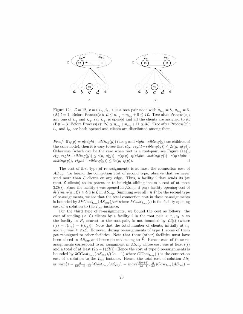
Figure 12: L = 12, x =< ir1 , ir2 > is a root-pair node with nir1 = 8, nir2 = 6.(A) t = 1. Before Process(x): L ≤ nir1 + nir2 + 9 ≤ 2L. Tree after Process(x):any one of ir1 and ir2 , say ir1 , is opened and all the clients are assigned to it;(B)t = 3. Before Process(x): 2L ≤ nir1 +nir2 +11 ≤ 3L. Tree after Process(x):ir1 and ir2 are both opened and clients are distributed among them.

Proof. If η(y) = η(right−sibling(y)) (i.e. y and right−sibling(y) are children ofthe same node), then it is easy to see that c(y, right−sibling(y)) ≤ 2c(y, η(y)).Otherwise (which can be the case when root is a root-pair, see Figure (14)),c(y, right−sibling(y)) ≤ c(y, η(y))+c(η(y), η(right−sibling(y)))+c(η(right−sibling(y)), right− sibling(y)) ≤ 3c(y, η(y)).

The cost of first type of re-assignments is at most the connection cost ofAScap. To bound the connection cost of second type, observe that we neversend more than L clients on any edge. Thus, a facility i that sends its (atmost L clients) to its parent or to its right sibling incurs a cost of at most3Ll(i). Since the facility i was opened in AScap, it pays facility opening cost ofδl(i)min{ni,L} ≥ δl(i)αL in AScap. Summing over all i ∈ P for the second typeof re-assignments, we see that the total connection cost in these re-assignmentsis bounded by 3FCostIcap

(AScap)/αδ where FCostIcap(.) is the facility opening

cost of a solution to the Icap instance.For the third type of re-assignments, we bound the cost as follows: the

cost of sending (< L) clients by a facility i in the root pair < r1, r2 > tothe facility in P , nearest to the root-pair, is not bounded by Ll(i) (wherel(i) = l(ir1) = l(ir2)). Note that the total number of clients, initially at ir1and ir2 was ≥ 2αL. However, during re-assignments of type 1, some of themgot reassigned to other facilities. Note that these (other) facilities must havebeen closed in AScap and hence do not belong to P . Hence, each of these re-assignments correspond to an assignment in AScap whose cost was at least l(i)and a total of at least (2α− 1)Ll(i). Hence the cost of type 3 re-assignments isbounded by 3CCostIcap(AScap)/(2α − 1) where CCostIcap(.) is the connectioncost of a solution to the Icap instance. Hence, the total cost of solution AS1

is max{1 + 3(2α−1) ,

3αδ}CostIcap(AScap) = max{ 2(α+1)

(2α−1) ,3αδ}CostIcap(AScap) =

20

Figure 13: L = 12, t = 1. x =< ir1 , ir2 > is a root-pair node with nir1 +nir2 +9 <L. Tree after Process(x).

Figure 14: c(y, right− sibling(y)) ≤ 3c(y, η(y))

2(α+1)(2α−1)CostIcap

(AScap) for δ = 3(2α−1)2α(α+1) .

Thus, the total cost of the solution is,CostI(S) ≤ CostI(St) + CostI1(AS1)

≤ O(1)CostI(O) + 2(α+1)(2α−1)CostIcap

(AScap)

≤ O(1)CostI(O) + 2(α+1)(5+ε)(2α−1) CostIcap

(Ocap)

≤ O(1)CostI(O) + 12(α+1)(2α−1) CostIcap

(Ocap)

≤ O(1)CostI(O) + 12(α+1)(1+2δ)(2α−1) CostI2(O2)

≤ O(1)CostI(O) + 12(α2+7α−3)α(2α−1) CostI2(O2)

= O(1)CostI(O) + 24(α2+7α−3)α(2α−1) CostI1(O1)

= O(1)CostI(O) + 24(α2+7α−3)α(2α−1) (CostI(S

t) + CostI(O))

= O(1)CostI(O) + 24(α2+7α−3)α(2α−1) (O(1)CostI(O))

= O(1)CostI(O)

21

6 Conclusion and Future Work

In this paper, we presented the first (constant) approximation algorithm forfacility location problem with uniform lower and upper bounds without violatingthe lower bounds. Upper bounds are violated by (5/2)-factor. Violation in theupper bound is less when the gap between the lower and the upper bound islarge. For example, if L ≤ U/2 then the upper bound violation is at mostβ + 1

2 ≤ 2.In future, if one can obtain a tri-criteria solution (with α > 1/2) when one

of the bounds is uniform and the other is non-uniform, then it can be simplyplugged into our technique to obtain similar result for the problem. When theupper bounds are non-uniform and τ = 1

maxi{Ui/L} then L ≤ τUi for all i and

τ ≤ 1. Also, violation in the upper bounds, then, is ≤ β + τ ≤ β + 1. Whenthe lower bounds are non-uniform and τ = 1

maxi{U/Li} then Li ≤ τU for all i

and τ ≤ 1. As before, violation in the upper bounds is ≤ β + τ ≤ β + 1. Notethat, for this case, we can not use the tri-criteria solution of Friggstad et al. [8]as α < 1/2 in their solution.

References

[1] Ankit Aggarwal, Anand Louis, Manisha Bansal, Naveen Garg, NeelimaGupta, Shubham Gupta, and Surabhi Jain. A 3-approximation algorithmfor the facility location problem with uniform capacities. Journal of Math-ematical Programming, 141(1-2):527–547, 2013.

[2] Sara Ahmadian and Chaitanya Swamy. Improved approximation guaran-tees for lower-bounded facility location. In Thomas Erlebach and GiuseppePersiano, editors, Approximation and Online Algorithms, pages 257–271,Berlin, Heidelberg, 2013. Springer Berlin Heidelberg.

[3] Hyung-Chan An, Mohit Singh, and Ola Svensson. Lp-based algorithms forcapacitated facility location. In FOCS, 2014, pages 256–265.

[4] Anna Arutyunova and Melanie Schmidt. Achieving anonymity via weaklower bound constraints for k-median and k-means, 2020.

[5] Manisha Bansal, Naveen Garg, and Neelima Gupta. A 5-approximation forcapacitated facility location. In Algorithms - ESA 2012 - 20th Annual Euro-pean Symposium, Ljubljana, Slovenia, September 10-12, 2012. Proceedings,pages 133–144, 2012.

[6] Jaroslaw Byrka, Krzysztof Fleszar, Bartosz Rybicki, and Joachim Spoer-hase. Bi-factor approximation algorithms for hard capacitated k -medianproblems. In SODA 2015, pages 722–736.

[7] Fabian A. Chudak and David P. Williamson. Improved approximationalgorithms for capacitated facility location problems. In Proceedings of

22

7th International Conference on Integer Programming and CombinatorialOptimization (IPCO), Graz, Austria,, pages 99–113, 1999.

[8] Zachary Friggstad, Mohsen Rezapour, and Mohammad R. Salavatipour.Approximating Connected Facility Location with Lower and Upper Boundsvia LP Rounding. In 15th Scandinavian Symposium and Workshops onAlgorithm Theory (SWAT 2016), volume 53 of Leibniz International Pro-ceedings in Informatics (LIPIcs), pages 1:1–1:14, Dagstuhl, Germany, 2016.Schloss Dagstuhl–Leibniz-Zentrum fuer Informatik.

[9] Sapna Grover, Neelima Gupta, Samir Khuller, and Aditya Pancholi. Con-stant factor approximation algorithm for uniform hard capacitated knap-sack median problem. In 38th IARCS Annual Conference on Foundationsof Software Technology and Theoretical Computer Science, FSTTCS 2018,December 11-13, 2018, Ahmedabad, India, volume 122 of LIPIcs, pages23:1–23:22. Schloss Dagstuhl - Leibniz-Zentrum fur Informatik, 2018.

[10] S. Guha, A. Meyerson, and K. Munagala. Hierarchical placement andnetwork design problems. In Proceedings of the 41st Annual Symposium onFoundations of Computer Science, FOCS ’00, page 603, USA, 2000. IEEEComputer Society.

[11] Yutian Guo, Junyu Huang, and Zhen Zhang. A constant factor approx-imation for lower-bounded k-median. In Jianer Chen, Qilong Feng, andJinhui Xu, editors, Theory and Applications of Models of Computation,pages 119–131, Cham, 2020. Springer International Publishing.

[12] Lu Han, Chunlin Hao, Chenchen Wu, and Zhenning Zhang. Approxima-tion algorithms for the lower-bounded k-median and its generalizations.In Donghyun Kim, R. N. Uma, Zhipeng Cai, and Dong Hoon Lee, edi-tors, Computing and Combinatorics, pages 627–639, Cham, 2020. SpringerInternational Publishing.

[13] D. R. Karger and M. Minkoff. Building steiner trees with incomplete globalknowledge. In Proceedings 41st Annual Symposium on Foundations of Com-puter Science, pages 613–623, 2000.

[14] Madhukar R. Korupolu, C. Greg Plaxton, and Rajmohan Rajaraman.Analysis of a local search heuristic for facility location problems. Jour-nal of Algorithms, 37(1):146–188, 2000.

[15] Retsef Levi, David B. Shmoys, and Chaitanya Swamy. Lp-based approxima-tion algorithms for capacitated facility location. Journal of MathematicalProgramming, 131(1-2):365–379, 2012.

[16] Shi Li. On facility location with general lower bounds. In SODA, pages2279–2290, 2019.

23

[17] Andrew Lim, Fan Wang, and Zhou xu. A transportation problem withminimum quantity commitment. Transportation Science, 40:117–129, 022006.

[18] Mohammad Mahdian and Martin Pal. Universal facility location. In Pro-ceedings of the 11th Annual European Symposium on Algorithms (ESA),Budapest, Hungary, volume 2832 of Lecture Notes in Computer Science,pages 409–421, 2003.

[19] M. Pal, E. Tardos, and T. Wexler. Facility location with nonuniform hardcapacities. In Proceedings of the 42nd IEEE Symposium on Foundationsof Computer Science (FOCS), Las Vegas, Nevada, USA, pages 329–338,2001.

[20] David B. Shmoys, Eva Tardos, and Karen Aardal. Approximation algo-rithms for facility location problems (extended abstract). In Proceedings ofthe Twenty-Ninth Annual ACM Symposium on the Theory of Computing,El Paso, Texas, USA,, pages 265–274, 1997.

[21] Zoya Svitkina. Lower-bounded facility location. ACM Trans. Algorithms,6(4), September 2010.

[22] Jiawei Zhang, Bo Chen, and Yinyu Ye. A multiexchange local search algo-rithm for the capacitated facility location problem. Journal of Mathematicsof Operations Research, 30(2):389–403, 2005.

24