first cosmology results using type ia supernova from the

MNRAS 485, 1171–1187 (2019) doi:10.1093/mnras/stz463Advance Access publication 2019 February 19

First cosmology results using Type Ia supernova from the Dark EnergySurvey: simulations to correct supernova distance biases

R. Kessler,1,2‹ D. Brout,3 C. B. D’Andrea,3 T. M. Davis,4 S. R. Hinton,4 A. G. Kim,5

J. Lasker,1,2 C. Lidman,6 E. Macaulay,7 A. Moller,6,8 M. Sako,3 D. Scolnic,2 M. Smith,9

M. Sullivan,9 B. Zhang,6,8 P. Andersen,4,10 J. Asorey,11 A. Avelino,12 J. Calcino,4

D. Carollo,13 P. Challis,12 M. Childress,9 A. Clocchiatti,14 S. Crawford,15,16

A. V. Filippenko,17,18 R. J. Foley,19 K. Glazebrook,20 J. K. Hoormann,4 E. Kasai,15,21

R. P. Kirshner,22,23 G. F. Lewis,24 K. S. Mandel,25 M. March,3 E. Morganson,26

D. Muthukrishna,6,8,27 P. Nugent,5 Y.-C. Pan,28,29 N. E. Sommer,6,8 E. Swann,7

R. C. Thomas,5 B. E. Tucker,6,8 S. A. Uddin,30 T. M. C. Abbott,31 S. Allam,32 J. Annis,32

S. Avila,7 M. Banerji,27,33 K. Bechtol,34 E. Bertin,35,36 D. Brooks,37 E. Buckley-Geer,32

D. L. Burke,38,39 A. Carnero Rosell,40,41 M. Carrasco Kind,26,42 J. Carretero,43

F. J. Castander,44,45 M. Crocce,44,45 L. N. da Costa,41,46 C. Davis,38 J. De Vicente,40

S. Desai,47 H. T. Diehl,32 P. Doel,37 T. F. Eifler,48,49 B. Flaugher,32 P. Fosalba,44,45

J. Frieman,2,32 J. Garcıa-Bellido,50 E. Gaztanaga,44,45 D. W. Gerdes,51,52 D. Gruen,38,39

R. A. Gruendl,26,42 G. Gutierrez,32 W. G. Hartley,37,53 D. L. Hollowood,19

K. Honscheid,54,55 D. J. James,56 M. W. G. Johnson,26 M. D. Johnson,26 E. Krause,48

K. Kuehn,57 N. Kuropatkin,32 O. Lahav,37 T. S. Li,2,32 M. Lima,41,58 J. L. Marshall,59

P. Martini,54,60 F. Menanteau,26,42 C. J. Miller,51,52 R. Miquel,43,61 B. Nord,32

A. A. Plazas,49 A. Roodman,38,39 E. Sanchez,40 V. Scarpine,32 R. Schindler,39

M. Schubnell,52 S. Serrano,44,45 I. Sevilla-Noarbe,40 M. Soares-Santos,62

F. Sobreira,41,63 E. Suchyta,64 G. Tarle,52 D. Thomas,7 A. R. Walker,31 and Y. Zhang32

DES CollaborationAffiliations are listed at the end of the paper

Accepted 2019 February 5. Received 2019 January 24; in original form 2018 November 7

ABSTRACTWe describe catalogue-level simulations of Type Ia supernova (SN Ia) light curves in the DarkEnergy Survey Supernova Program (DES-SN) and in low-redshift samples from the Center forAstrophysics (CfA) and the Carnegie Supernova Project (CSP). These simulations are used tomodel biases from selection effects and light-curve analysis and to determine bias correctionsfor SN Ia distance moduli that are used to measure cosmological parameters. To generaterealistic light curves, the simulation uses a detailed SN Ia model, incorporates information fromobservations (point spread function, sky noise, zero-point), and uses summary information(e.g. detection efficiency versus signal-to-noise ratio) based on 10 000 fake SN light curveswhose fluxes were overlaid on images and processed with our analysis pipelines. The quality ofthe simulation is illustrated by predicting distributions observed in the data. Averaging withinredshift bins, we find distance modulus biases up to 0.05 mag over the redshift ranges of the

� E-mail: [email protected]

C© 2019 The Author(s)Published by Oxford University Press on behalf of the Royal Astronomical Society

Dow

nloaded from https://academ

ic.oup.com/m

nras/article/485/1/1171/5342076 by SBD-FFLC

H-U

SP user on 21 Decem

ber 2020

mailto:[email protected]

1172 DES Collaboration

low-z and DES-SN samples. For individual events, particularly those with extreme red or bluecolour, distance biases can reach 0.4 mag. Therefore, accurately determining bias correctionsis critical for precision measurements of cosmological parameters. Files used to make thesecorrections are available at https://des.ncsa.illinois.edu/releases/sn.

Key words: techniques – cosmology – supernovae – (cosmology:) dark energy.

1 IN T RO D U C T I O N

Since the discovery of cosmic acceleration (Riess et al. 1998;Perlmutter et al. 1999) using a few dozen Type Ia supernovae(SNe Ia), surveys have been collecting larger SN Ia samples andimproving the measurement precision of the dark energy equationof state parameter (w). This improvement is in large part due to theuse of rolling surveys to discover and measure large numbers ofSN Ia light curves in multiple passbands with the same instrument.The most recent Pantheon sample (Scolnic et al. 2018a) includesmore than 1000 spectroscopically confirmed SNe Ia from low- andhigh-redshift surveys. Compared to the 20th century sample used todiscover cosmic acceleration, the Pantheon sample has more than a20-fold increase in statistics and much higher quality light curves.

In addition to improving statistics and light-curve quality, reduc-ing systematic uncertainties is equally important. While most of theattention is on calibration, which is the largest source of systematicuncertainty, significant effort over more than a decade has gone intomaking robust simulations that are used to correct for the redshift-dependent distance-modulus bias (μ-bias) arising from selectioneffects. Selection effects include several sources of experimentalinefficiencies: instrumental magnitude limits resulting in Malmquistbias, detection requirements from an image-subtraction pipelineused to discover transients, target selection for spectroscopic follow-up, and cosmology-analysis requirements. These selection effectsintroduce average μ-bias variations reaching ∼0.05 mag at the high-redshift range of a survey [e.g. see fig. 5 in Betoule et al. (2014) andfig. 6 in Scolnic et al. (2018a)], and the μ-bias averaged in specificcolour ranges can be an order of magnitude larger.

In addition to sample selection, the μ-bias depends on the parentpopulations of the SN Ia stretch and colour, and also on intrinsicbrightness variations, hereafter called ‘intrinsic scatter’, both in theabsolute magnitude and in the colours. For precision measurementsof cosmological parameters, simulations are essential to determineμ-bias corrections, and these simulations require accurate modelsof SN light curves and sample selection.

The main focus of this paper is to describe our simulations ofspectroscopically confirmed SNe Ia from three seasons of the DarkEnergy Survey Supernova Program (DES-SN), and the associatedlow-z sample. The combination of these two samples, called DES-SN3YR, is used to measure cosmological parameters presented inDES Collaboration et al. (2018). All simulations were performedwith the public ‘SuperNova ANAlysis’ (SNANA) software package(Kessler et al. 2009b).1 In addition to SNe Ia, a variety of sourcemodels can be supplied to the SNANA simulation, including corecollapse (CC) SNe, kilonovae (KN), or any rest-frame modeldescribed by a time-dependent sequence of SEDs.

The SNANA simulations are performed at the ‘catalogue level’,which means that rather than simulating SN light curves on images,light-curve fluxes and uncertainties are computed from imageproperties. The simulation inputs include a rest-frame source model,volumetric rate versus redshift, cosmological parameters (e.g.

1https://snana.uchicago.edu

�M and w), telescope transmission in each passband, calibrationreference, observing and image properties from a survey, andrandom numbers to generate Poisson fluctuations. The simulatedlight curves are treated like calibrated light curves from a surveyand are thus analysed with the same software as for the data.

The SNANA simulation is ideally suited for rolling searches inwhich the same instrument is used for both discovery and formeasuring light curves. Surveys with rolling searches include theSupernova Legacy Survey (SNLS; Astier et al. 2006), the SloanDigital Sky Survey-II (SDSS-II; Frieman et al. 2008; Sako et al.2018), the Panoramic Survey Telescope and Rapid Response System(PS1 Kaiser et al. 2002), and DES. The low-z sample, however, isbased on follow-up observations from independent search programs(CFA, CSP; Hicken et al. 2009, 2012; Contreras et al. 2010; Folatelliet al. 2010), and the observing properties of the search are notavailable to perform a proper simulation. The low-z simulation,therefore, requires additional assumptions and approximations.

Simulated corrections first appeared in the SNLS cosmologyanalysis (Astier et al. 2006). Kessler et al. (2009a) analysedseveral samples (low-z, SDSS-II, SNLS, ESSENCE), which ledto a more general SNANA framework to simulate μ-bias correctionsfor arbitrary surveys. The heart of this framework is a set of twolibraries. First, an observation library where each observation dateincludes a characterization of the point spread function (PSF), skyand readout noise, template noise, zero-point, and gain. Secondly,a host-galaxy library includes magnitudes and surface profiles, andis used to compute Poisson noise and to model the local surfacebrightness. For a specified light-curve model, these libraries are usedto convert top-of-the-atmosphere model magnitudes into observedfluxes and uncertainties.

After a survey has completed, assembling the libraries is arelatively straightforward exercise, and SNANA simulations havebeen used in numerous cosmology analyses (Kessler et al. 2009a;Conley et al. 2011; Betoule et al. 2014; Rest et al. 2014; Scolnic et al.2014a, 2018a). Before a survey has started, predicting the librariesis one of the critical tasks for making reliable forecasts. Such pre-survey forecasts with the SNANA simulation have been made forLSST2 (LSST Science Collaboration et al. 2009; Kessler et al.2010b), DES-SN (Bernstein et al. 2012), and WFIRST3 (Hounsellet al. 2018).

While our main focus is to describe the DES-SN3YR simulationof SNe Ia, and how a large (∼106 events) simulated bias-correctionsample is used to model biases in the measured distance modulus,it is worth noting other applications from the flexibility in SNANA.First, these simulations are used to generate 100 data-sized DES-SN3YR validation samples that are processed with the same biascorrections and cosmology analysis used on the data. This validationtest is used to accurately check for w-biases at the ∼0.01 level,and to compare the spread in w values with the fitted uncertainty(Brout et al. 2018b). The validation and bias-correction samples

2Large Synoptic Survey Telescope: https://www.lsst.org.3Wide Field Infrared Space Telescope: https://wfirst.gsfc.nasa.gov.

MNRAS 485, 1171–1187 (2019)

Dow


ic.oup.com/m


H-U

SP user on 21 Decem

ber 2020

https://des.ncsa.illinois.edu/releases/sn

https://snana.uchicago.edu

https://www.lsst.org

https://wfirst.gsfc.nasa.gov

Simulations to correct SN Ia distance biases 1173

are generated with the same code and options, but are used fordifferent tasks. Other applications include CC simulations for aclassification challenge (Kessler et al. 2010a), CC simulations for aPS1 cosmology analysis using photometrically identified SNe Ia(Jones et al. 2017, 2018), simulating the KN search efficiency(Soares-Santos et al. 2016; Doctor et al. 2017), and making KNdiscovery predictions for 11 past, current, and future surveys(Scolnic et al. 2018b).

In this work, we describe the simulation from a scientific perspec-tive without instructions on implementation. For implementation,we refer to the manual available from the SNANA homepage,and recommend contacting community members familiar with thesoftware. This simulation is possible because of extensive publiclyavailable resources. When using this simulation in a publication, werecommend the added effort of referencing the relevant underlyingcontributions, such as the source of models or data samples used tomake templates.

The organization of this paper is as follows. The DES-SN3YRsample is described in Section 2. An overview of the simulationmethod is in Section 3, and fake SN light curves overlaid on imagesis described in Section 4. Modelling is described in Section 5 forSNe Ia light-curve magnitudes, Section 6 for fluxes and uncertain-ties, and Section 7 for the trigger. The quality of the simulationis illustrated with data/simulation comparisons in Section 8, andredshift-dependent μ-biases are described in Section 9. We concludein Section 10, and present additional simulation features in theAppendix.

2 DATA SAMPLES

Here, we describe the data samples that are simulated for the cos-mology analysis in DES Collaboration et al. (2018) and Brout et al.(2018b). After selection, this sample includes 207 spectroscopicallyconfirmed SNe Ia from the first three seasons (2013 August through2016 February) of DES-SN (Diehl et al. 2016), and 122 low-z(z < 0.1) SNe Ia from CFA3 (Hicken et al. 2009), CFA4 (Hickenet al. 2012), and CSP (Contreras et al. 2010; Folatelli et al. 2010).This combined sample of 329 SNe Ia is called ‘DES-SN3YR’.

The DES-SN sample was acquired in rolling search mode usingthe 570 Megapixel Dark Energy Camera (DECam; Flaugher et al.2015) mounted on the 4-m Blanco telescope at the Cerro TololoInter-American Observatory (CTIO). Ten 2.7 deg2 fields wereobserved in g, r, i, z broad-band filters, with a cadence of roughly1 week in each band. Defining single-visit depth as the magnitudewhere the detection efficiency is 50 per cent, eight of these fieldshave an average single-visit depth of ∼23.5 mag (hereafter called‘shallow’ fields), and the remaining two fields have a depth of∼24.5 mag (hereafter called ‘deep’ fields).

SNe Ia are detected by a difference-imaging pipeline (DiffImg)described in Kessler et al. (2015), and the spectroscopic selection isdescribed in D’Andrea et al. (2018). The instrumental photometricprecision from DiffImg is limited at the 2 per cent level, andtherefore a separate and more accurate ‘Scene Model Photometry(SMP)’ pipeline (Brout et al. 2018a) is used to measure the light-curve fluxes and uncertainties for the cosmology analysis. For eachevent, SMP simultaneously fits a 30 × 30 pixel-grid flux modelto each observation, where the model includes a time-independentgalaxy flux and a time-dependent source flux, each convolved withthe PSF.

In addition to SN Ia light curves, the DES-SN data include other‘meta-data’ for monitoring, calibration (e.g. telescope transmis-sions), and analysis. An important meta-data product for simulations

is from the fluxes of ∼10 000 ‘fake’ SN light curves overlaid onthe images during the survey (Section 4), and processed in real timealong with the data to find SN candidates with DiffImg.

The low-z sample includes redshifts, light-curve fluxes, fluxuncertainties, and filter transmission functions. The photometry,however, is not from a rolling search but is from follow-upprogrammes that target SNe Ia discovered from other search pro-grammes such as LOSS (Ganeshalingam, Li & Filippenko 2013).Since the observation information from the search programmes isnot available, the resulting observation library is an approximationbased on several assumptions (Section 6.1.1).

3 OV E RV I E W O F B I A S C O R R E C T I O N S A N DSI MULATI ON

The primary goal of our simulation is to provide inputs to the‘BEAMS with Bias Correction (BBC)’ method (Kessler & Scolnic2017), which is the stage in our cosmology analysis that produces abias-corrected SN Ia Hubble diagram (section 3.8.1 of Brout et al.2018b). A large simulated bias-correction sample is fit with theSALT-II light-curve model, in the same way as for the data, toproduce three parameters for each event: amplitude (x0), stretch(x1), and colour (c). A statistical comparison of the fitted and trueparameters is used to determine a bias correction for each parameteron a five-dimensional (5D) grid of {z, x1, c, α, β}, where z isthe redshift, x1 and c are SALT-II-fitted parameters, and α and β

are SALT-II standardization parameters (Section 5.3). BBC usesthe 5D grid to bias-correct each set of SALT-II parameters fromthe data, and these corrected parameters are used to determine abias-corrected distance modulus.

A schematic illustration of the SNANA simulation is shown inFig. 1. The left column illustrates the generation of the sourcespectral energy distribution (SED) and astrophysical effects. Theseeffects include host-galaxy extinction, redshifting, cosmologicaldimming, lensing magnification, peculiar velocity, and Milky Wayextinction. The output of this column is a true magnitude at the topof the atmosphere.

The middle column of Fig. 1 illustrates the instrumental simula-tion, where the true magnitude is converted into an observed numberof charged coupled device (CCD) counts, hereafter denoted ‘flux’,and the uncertainty on the flux. The observation information (PSF,sky noise, zero-point) and host-galaxy profile are used to computethe Poisson noise.

The right column in Fig. 1 illustrates the simulation of thetrigger that selects events for analysis. Epochs that result in adetection, which is roughly a 5σ excess on the subtracted image(Section 7.1), are processed with additional logic to identify andstore ‘candidates’ for analysis. The candidate logic specifies howmany detections, from which band(s) the detection must occur,and the minimum time separation between detections. Finally, thetrigger includes a selection function for the subset of candidates thatwere spectroscopically confirmed.

The noise and trigger models in Fig. 1 each have inputs basedon analysing artificial light curves overlaid on CCD images. These‘fakes’ are described in Section 4.

4 FA K E SN IA L I G H T C U RV E S OV E R L A I D O NIMAG ES

Ideally, simulated bias corrections would be based on SN Ialight-curve fluxes overlaid on to CCD images and processed withexactly the same software as the data. CPU resources for so many

MNRAS 485, 1171–1187 (2019)

Dow


ic.oup.com/m


H-U

SP user on 21 Decem

ber 2020


Figure 1. Flow chart of SNANA simulation.

image-based simulations, however, would be enormous. Kessleret al. (2015) estimates that SNANA simulations are × 105 faster thanimage-based simulations, while still producing realistic light-curvefluxes and uncertainties. Although we do not perform image-basedsimulations for bias corrections, we use image simulations to informthe SNANA simulation. Specifically, 10 000 ‘fake’ SN light curveswere overlaid on DES-SN images and processed through the samepipelines as the data, including difference imaging (DiffImg;Kessler et al. 2015) and photometry (Brout et al. 2018a) pipelines.For DiffImg, these fakes are used to measure the detectionefficiency versus signal-to-noise ratio (SNR), which is needed forthe trigger model in Fig. 1. For the photometry pipeline, fakes areused to measure the rms scatter between measured and true fluxes,and the rms is used to determine scale factors for the SN fluxuncertainties (noise model in Fig. 1).

Prior to the start of DES operations, the fake light-curve fluxeswere computed from the SNANA simulation using the populationof stretch and colour (Section 5.1) from Kessler et al. (2013), andintrinsic scatter (Section 5.2) was ignored to simplify the analyseswith fakes. The redshift distribution (0.1 < z < 1.4) is described bya polynomial function of redshift, and was tuned to acquire goodstatistics over the full redshift range and thus span the full range ofSN magnitudes. Each fake location is selected on top of a randomgalaxy as described in Section 6.2. The SN model flux is distributedamong pixels using the position-dependent PSF, and the flux in eachpixel includes Poisson fluctuations from the sky background and thesource.

The galaxy occupation fraction was limited to ∼1 per cent ineach 0.05-wide redshift bin because the DES-SN search pipelineprocessed only one set of images, which included fakes, and a fakeevent overlaid on a galaxy prevents a real transient detection onthat galaxy in the same season, but allows real events in futureseasons where the fake is not overlaid. Once a real transient event isassociated with a galaxy, fakes will not be overlaid on that galaxy.

Since the SMP pipeline performs a global fit to all images, accurateastrometry is needed to overlay the fake light-curve flux at the samesky location for each exposure. As described in Brout et al. (2018a),our astrometric precision results in ∼0.001 mag uncertainties forreal sources, and thus the astrometric precision is adequate for thefakes.

Since the goal with fakes is to characterize single-epoch featuresof the CPU intensive image-processing pipelines and to input thesefeatures into the much faster SNANA simulation, the choice ofSN light-curve model does not matter as long as the fake modelmagnitudes span the same range as the data. The resulting SNANA

simulation can be used to simulate arbitrary light-curve modelsand redshift dependence. For example, to evaluate systematicuncertainties in this analysis, we simulate SNe Ia with differentmodels of intrinsic scatter and with different populations of stretchand colour.

While this seemingly large sample of SN fakes is used tocharacterize image-processing features, these fakes cannot be usedto compute μ-bias corrections for two reasons. First, the light-curvemodel used to generate fakes is deliberately different from reality forpractical reasons explained above. Secondly, 10 000 fakes is morethan an order of magnitude smaller than what is needed for thebias-correction sample used in the BBC method (Kessler & Scolnic2017). In addition, even if an accurate SN Ia model were used togenerate fakes, the resulting efficiency and bias corrections wouldbe valid only for that particular SN Ia model, and not applicableto other SN Ia models, nor to transient models such as CC SNe orKNe.

5 SO U R C E M O D E L

Here, we describe the simulation components under ‘Source Model’in Fig. 1. This includes the generation of the SN Ia SED as a functionof time, how the SEDs are altered as the light travels from the source

MNRAS 485, 1171–1187 (2019)

Dow


ic.oup.com/m


H-U

SP user on 21 Decem

ber 2020


to Earth, and how each SED is transformed into a model magnitudeabove the atmosphere.

5.1 SN Ia light-curve model

To simulate SNe Ia, we use the SALT-II SED model described inGuy et al. (2010), and the trained model from the Joint LightcurveAnalysis (JLA) (Betoule et al. 2014). The underlying model isa rest-frame SED with wavelengths spanning 2000–9200 Å, andrest-frame epochs spanning −20 < Trest < +50 d with respect tothe epoch of peak brightness. For each event there are four SN-dependent parameters generated by the simulation:

(i) time of peak brightness, t0, randomly selected between2 months before the survey begins and one month after the surveyends.

(ii) SALT-II colour parameter, c.(iii) SALT-II stretch parameter, x1.(iv) CMB frame redshift, zcmb, true, selected from the rate model

in Section 5.7 .

The rest-frame SED depends on the colour and stretch param-eters. For each epoch, the SED undergoes cosmological dimming(Section 5.4), is redshifted (Section 5.5) to the observer frame, andfinally multiplied by the filter transmission function to producegenerated fluxes and magnitudes. Wavelength-dependent MilkyWay extinction (Section 5.6) is included in the flux-integrals,and thus the generated magnitudes are top-of-the-atmosphere. Forepochs past 50 d, magnitudes are linearly extrapolated as a functionof Trest. For light-curve fitting we use epochs satisfying −15 < Trest

< 45 d, but we simulate epochs outside this Trest range to accountfor uncertainty in the fitted t0, which increases the true Trest range.

The SALT-II amplitude parameter, x0, is computed using theestimator in Tripp (1998),

log10(x0) = −0.4(μmodel + μlens − αx1 + βc − M), (1)

where μmodel is the distance modulus (Section 5.4) which dependson cosmology parameters, μlens is due to lensing magnification(Section 5.4), α and β are SALT-II standardization parameters(Section 5.3), and M = −19.365 is a reference magnitude. It iswell known that M is degenerate with the Hubble constant (H0),and that their values have no impact in the SN Ia analysis ofcosmological parameters. However, the quality of the simulationdepends on predicting accurate observer-frame magnitudes, andtherefore M + 5 log10(H0) must be well determined. The SALT-IISED is redshifted using the heliocentric redshift (zhel, true), whichis transformed from zcmb, true using the sky coordinates from theobservation library. zhel, true also includes a random host-galaxypeculiar velocity described in Section 5.5.

5.2 Intrinsic scatter

Before redshifting the SALT-II SED, intrinsic scatter is applied asspectral variations to the SED. To evaluate systematic uncertaintiesin the bias corrections, two different models are used that approxi-mately span the range of possibilities in current data samples. Firstis the ‘G10’ model (Guy et al. 2010) from the SALT-II trainingprocess. Roughly 75 per cent of the scatter is coherent amongall wavelengths and epochs, while the remaining 25 per cent ofthe scatter results from colour variations that are not correlatedwith luminosity. The second model, ‘C11’, is based on broad-band (UBVRI) covariances found in Chotard et al. (2011). Only

25 per cent of the scatter is coherent, while the remaining scatterresults from colour variations. Details of these models are given inKessler et al. (2013), and both models result in 0.13 mag intrinsicscatter on the Hubble diagram.4

5.3 Global SALT-II model parameters

While the SALT-II SED and colour law model parameters from thetraining process are fixed for each SN, there are a few parametersthat are determined outside the training process. To simulatevalidation data samples, the standardization parameters are: α =0.15, βG10 = 3.1, and βC11 = 3.8, where G10 and C11 refer to theintrinsic scatter model (Section 5.2). The standardization parametersfor the μ-bias simulations are defined on a 2 × 2 grid to enable BBCinterpolation of the μ-bias as a function of α and β; this is describedin Section 9.

For the population of stretch (x1) and colour (c), we use theasymmetric Gaussian parametrization from Scolnic & Kessler(2016, hereafter SK16). For DES-SN stretch & colour, we use thehigh-z G10 and C11 rows from table 1 of SK16. For the low-zsample we use the colour population parameters from the low-zrow of table 1 of SK16. The stretch population is double-peaked,and we use the parametrization from appendix C of Scolnic et al.(2018a). While we account for the colour and stretch populationdifferences between low-z and DES-SN, the redshift dependence ofthe population has not been quantified and therefore is not includedin our simulations.

5.4 Luminosity distance and lensing magnification

The luminosity distance (DL) for a flat universe is computed as

DL = (1 + zhel,true)c

H0

∫ zcmb,true

0dz/E(z),

E(z) = [��(1 + z)3(1+w) + �M(1 + z)3

]1/2, (2)

where �M is today’s matter density, �� is today’s dark energydensity, and w is the dark energy equation of state parameter. Notethat both the CMB and heliocentric redshifts are used to computeDL, but the 1 + zhel,true pre-factor is an approximation: the exact pre-factor is 1 + zobs, where zobs is the measured redshift (Davis et al.2011). However, we do not simulate Earth’s motion around our Sun,nor the local SN motion within its host galaxy, and therefore zobs =zhel, true. The error on DL from ignoring local motions is less than10−3. To compute E(z) in our simulations we set H0 = 70 km s−1,5

�� = 0.7, �M = 0.3, and w = −1. The distance modulus (μmodel

in equation 1) is defined as μmodel = 5log10(DL/10 pc).Weak lensing effects are described by the μlens term in equa-

tion (1), and modelled as follows:

(i) 0.4 < z < 1.4: A convergence (κ) distribution is determinedfrom a 900 deg2 patch of the MICECAT N-body simulation (Crocceet al. 2015).6 Galaxies are from a halo occupation distribution anda sub-halo abundance matching technique (Carretero et al. 2015).

4This 0.13 mag scatter is larger than typical fitted σ int values of 0.1 magbecause of SALT-II model uncertainties; see section 7.1 of Kessler & Scolnic(2017) for explanation.5This H0 value was used in the SN Ia model training, which determinesthe absolute brightness M, and therefore the simulated H0 should not beupdated with more recent measurements.6https://cosmohub.pic.es

MNRAS 485, 1171–1187 (2019)

Dow


ic.oup.com/m


H-U

SP user on 21 Decem

ber 2020

https://cosmohub.pic.es


The lensing distribution is determined from μlens = 5log10(1 − κ)(shear contribution is negligible and ignored).

(ii) z < 0.4: Using the MICECAT approach above to determineμlens at z = 0.4 (μlens,0.4), the lensing at lower redshifts is computedas

μlens,z = μlens,0.4 × z/0.4. (3)

As a crosscheck, this z-scale approximation works well within theMICECAT redshift range: e.g. μlens, 0.4 � μlens, 0.6 × (0.4/0.6).

The root mean square (rms) scatter in the model μlens distributionis approximately 0.05 × z. For systematic studies, the simulationincludes an option to scale the width of the distribution to increaseor decrease the scatter.

To properly select from the asymmetric μlens distribution, insteadof a Gaussian approximation, the lensing magnification probabilityis defined as a two-dimensional (2D) function of redshift and μlens.For each simulated redshift, a random μlens is selected from theμlens probability distribution. While our lensing model accounts forlarge scale structure on average, it does not account for correlationsbetween events with small angular separations.

5.5 Peculiar velocity and observed redshift

The generated CMB-frame redshift, zcmb,true, is transformed to theheliocentric frame, zhel,true, using the sky coordinates from theobservation library. The redshift observed in the heliocentric frameis

zhel,obs = (1 + zhel,true)(1 + vpec/c − vpec,cor/c) − 1

+δznoise (4)

= (1 + zhel,true)(1 − vpec,err/c) − 1

+δznoise, (5)

where vpec is a peculiar velocity randomly chosen from a Gaussianprofile with σ vpec = 300 km s−1, and δznoise is a measurement error.For DES-SN and low-z, δznoise is drawn from a Gaussian with σ z =10−4.

While the peculiar velocity model is the same for low-z andDES-SN, corrections are modelled only for the low-z sample. Thesimulated low-z correction simply reduces the vpec scatter withoutapplying real corrections. Following the Pantheon analysis (Scolnicet al. 2018a), vpec,cor = vpec + vpec,err where vpec,err is a randomlyselected error from a Gaussian profile with a 250 km s−1 sigma.Finally, zhel, obs is transformed back to the CMB frame redshift,zcmb,obs. Peculiar velocity corrections for DES-SN can be computedin principle, but such corrections on a high-redshift sample arenegligible and were thus ignored.

5.6 Galactic extinction

For each simulated event the Galactic extinction parameter,E(B − V), is computed from the maps in Schlegel, Finkbeiner &Davis (1998). Following a stellar analysis from SDSS (Schlafly &Finkbeiner 2011), we scale the E(B − V) values by 0.86. We assumethe reddening law derived in Fitzpatrick (1999), and with AV definedas the extinction at 5500 Å, RV ≡ AV/E(B − V) = 3.1.

5.7 Volumetric rate model

The redshift distribution of SNe Ia is generated from a co-movingvolumetric rate, R(z), measured by SNLS (Perrett et al. 2012):

R(z) = 1.75 × 10−5(1 + z)2.11 yr−1Mpc−3, (6)

and is valid up to redshift z < 1.

6 MO D E L L I N G FL U X A N D N O I S E

Here we describe the simulation components under ‘Noise Model’in Fig. 1. There are two steps needed to simulate flux and noise.First, an observation library is needed to characterize observingconditions (Section 6.1). Next, each true model magnitude isconverted into a measured flux (CCD counts) and uncertainty(Section 6.3).

6.1 Observation library

An observation library is a collection of sky locations, each specifiedby right ascension (RA) and declination (Dec.), along with a list ofobservations for each location. For a small survey area, a single skylocation may be adequate, particularly for making forecasts. Fora proper simulation, however, many sky locations should be usedwith either random sampling or a grid. For DES-SN we use ∼104

random sky locations covering 27 deg2, which averages over densityfluctuations to achieve a representative sample for a homogeneousuniverse. For simulations with more than 104 generated events, thelibrary sky locations and observations are re-used with SNe that havea different set of randomly chosen properties. Since ∼1 per cent ofthe DES-SN events occur in the overlap between two adjacent fields,and thus have double the number of observations, the simulationincludes a mechanism to handle overlapping fields.

The exposure information for each sky location is defined asfollows:

(i) MJD is the modified Julian date.(ii) FILTER is the filter passband.(iii) GAIN is the number of photoelectrons per ADU.7

(iv) SKYSIG is the sky noise, including read noise.(v) σPSF = √

NEA /4π is an effective Gaussian σ for the PSF,and NEA is the noise-equivalent area defined as

NEA =[

2π∫

[PSF(r)]2r dr

]−1

. (7)

For a PSF-fitted flux, the fitted flux variance is the sky noise perpixel multiplied by NEA.

(vi) ZPTADU is the zero-point (ADU), and includes telescopeand atmospheric transmission.

Many of the DES-SN visits include multiple exposures: two z-band exposures in each of the eight shallow fields,8 and the twodeep fields include 3, 3, 5, 11 exposures for g, r, i, z bands,respectively. During the survey, DiffImg performs the searchon co-added exposures. In the analysis, SMP determines the fluxfor each individual exposure, and the fluxes are co-added at thecatalogue level. The co-adding for both DiffImg and SMP aretreated the same in the simulation by co-adding the observation

7ADU: Analogue to Digital Unit.8Shallow g, r, i include one exposure per visit.

MNRAS 485, 1171–1187 (2019)

Dow


ic.oup.com/m


H-U

SP user on 21 Decem

ber 2020


library information as follows:

MJD =[∑

MJDi

]/Nexpose,

SKYSIG =√∑

SKYSIG2i ,

σPSF =[∑

σPSFi

]/Nexpose,

ZPTADU = 2.5 × log10

[∑10(0.4·ZPTADUi )

], (8)

where Nexpose is the number of exposures and each sum includes i =1, Nexpose. ZPTADU is an approximation assuming the same GAINfor each exposure; the DES GAIN variations are a few per cent.

The randomly selected time of peak brightness (t0, Section 5.1),along with the light-curve time-window, determine the MJD-overlapin the observation sequence.

6.1.1 Observation library for low-z sample

The low-z sample does not include the observation properties(PSF, sky noise, zero-point) from their image-processing pipelines.Therefore, we construct an approximate library from the low-z lightcurves, using their sky locations, observation dates, and SNR. Thereis not enough light-curve information to uniquely determine theobservation properties, and therefore we use three assumptions: (1)fix eachGAIN to unity, (2) fix each PSF to 1 arcsec (full width at half-maximum), and (3) use a previously determined set of broad-bandsky magnitudes, and interpolate the sky magnitude to the centralwavelength of each simulated filter. For ground-based surveys, weuse the average sky mags in ugrizY passbands from a simulationof LSST (Delgado et al. 2014). The ZPTADU parameter is adjustednumerically so that the calculated SNR matches the observed SNR.

Another subtlety is that the low-z sample was collected overdecades, and thus for a randomly selected explosion time thereis little chance that the simulated light curve would overlap theobservation dates. To generate low-z light curves more efficiently,the measured time of peak brightness (t0) for each light curve isused for the corresponding sky location, thus ensuring a light curvewill be generated. Other SN properties (redshift, colour, stretch,intrinsic scatter) are randomly selected in the same way as for theDES-SN simulation.

6.2 Host-galaxy model

Host galaxies are used for two purposes in the SNANA simulationsof DES-SN. First, fakes are generated to be overlaid on top ofgalaxies in real CCD images. Secondly, to simulate bias correctionsand validation samples in the analysis, the local surface brightnessfrom the host is used to add Poisson noise and anomalous scatter(Fig. 2) in the light-curve fluxes. We do not simulate low-z hostgalaxies because the cadence library is constructed from observedSNR that should already include Poisson noise from the host. Whileanomalous scatter in the low-z sample may be present, the localsurface brightness information is not available to study this effect.9

For DES-SN the SNANA simulation uses a host-galaxy library(HOSTLIB), where each galaxy is described by (1) heliocentricredshift, zHOST,hel, (2) coordinates of the galaxy centre, (3) observer-frame magnitudes in the survey bandpasses, and (4) Sersic profile

9It would be a valuable community contribution to use public survey data(e.g. PS1, SDSS, and DES) and determine the local surface brightness foreach low-z event.

Figure 2. Simulated uncertainty scale, Ssim, as a function of local surfacebrightness mag (SB mag). Each panel indicates the set of fields and passband.Left-hand panels are for the deep SN fields (depth per visit ∼24.5); right-hand panels are for shallow SN fields (depth per visit ∼23.5).

with index n = 0.5 (Gaussian), and half-light radii along the majorand semimajor axes. The HOSTLIB can be created from data orfrom an astrophysical simulation. Our DES-SN simulation uses agalaxy catalogue derived from the DES science verification (SV)data, as described in Gupta et al. (2016). Eventually this galaxycatalogue will be updated using a much deeper co-add from the fullDES data set.

There are two caveats about this HOSTLIB. First, zHOST,hel

are photometric redshifts (photo-z). Extreme photo-z outliers arerejected by requiring the absolute r and i band magnitudes (Mr,i) tosatisfy −23 < Mr,i < −16, where Mr,i = mr,i − μphot, mr,i are theobserved magnitues, and μphot is the distance modulus computedfrom the photo-z. The second caveat is that the measured half-lightradii were scaled by a factor of 0.8 to obtain better data-simulationagreement in the surface brightness distribution (Section 8).

To generate fakes to overlay on images, each SN was associatedwith a random HOSTLIB event satisfying

|zSN,hel − zHOST,hel| < 0.01 + 0.05zSN, (9)

where zSN,hel and zHOST,hel are the heliocentric redshifts for the SNand host galaxy, respectively. The SN redshift is updated to zHOST,hel,the CMB-frame redshift (zcmb,true) is computed from zHOST,hel, andthe resulting zcmb,true is used to update the distance modulus andlight-curve magnitudes. To avoid multiple fakes around a singlegalaxy, each HOSTLIB event can be used only once. The SNcoordinates are chosen near the host, weighted by the Sersic profile.

To simulate samples for the analysis, the redshift matchingbetween the SN and the host is the same as for fakes (equation 9).However, the generated SN redshift (from rate model) and itscoordinates (from cadence library) are preserved. A random locationnear the host is selected from the Sersic profile and is used todetermine the local surface brightness and to add Poisson noiseto the light curves. The Poisson noise variance is computed byintegrating the host-galaxy flux over the noise equivalent area(equation 7). In this implementation of the DES-SN simulation,the host-galaxy spatial distribution is homogeneous on all scales.

MNRAS 485, 1171–1187 (2019)

Dow


ic.oup.com/m


H-U

SP user on 21 Decem

ber 2020


Large-scale structure can be incorporated as explained in theAppendix.

6.3 Converting true magnitudes into measured fluxes anduncertainties

Here, we describe how a true source magnitude at the top of theatmosphere, mtrue, is used to determine the instrumental flux andits uncertainty. The flux unit for this discussion is photoelectrons,but the simulation uses the GAIN to properly digitize the signals inADU.

The true flux is given by

Ftrue = 100.4(mtrue−ZPTpe), (10)

where ZPTpe = ZPTADU + 2.5 log10(GAIN) is the zero-point inunits of photoelectrons.

The true Poisson noise for the measured flux is given by

σ 2Ftrue = [Ftrue + (NEA · b) + σ 2

host]S2sim , (11)

where

(i) Ftrue is the true flux;(ii) NEA is the noise equivalent area (equation 7);(iii) b is the background per unit area (includes sky and CCD

read noise);(iv) σ host is Poisson noise from the underlying host galaxy

(Section 6.2);(v) Ssim is an empirically determined scale (Section 6.4) that

increases both the flux scatter and measured uncertainty.

NEA, b, and σPSF are obtained from the observation library(Section 6.1). Ssim is determined from analysing the fakes (Sec-tion 6.4) and characterizes subtle scene model photometry (SMP)behaviour that cannot be computed from first principles, mainly theanomalous flux scatter from bright galaxies. Because of the largenumber of reference images used in SMP, we do not include anexplicit template noise term.

For PSF-fitted fluxes, the noise estimate in equation (11) is anapproximation that is more accurate for sky-dominated noise, oras Ftrue/(NEA · b) becomes smaller. In principle, equation (11) isalso accurate for bright events with high SNR, but brighter SNeare associated with brighter galaxies that introduce anomalous fluxscatter. In Section 6.4, we use fakes to show how the simulatedflux uncertainties are corrected for anomalous scatter so that theuncertainties are accurate over the full range of SNR.

The true uncertainty (σ Ftrue) is used to select a random fluctuationon the true flux (Ftrue), resulting in the observed flux, F. Themeasured uncertainty for data is not the true uncertainty, but ratheran approximation based on the observed flux. In the simulation, themeasured uncertainty, σ F, is computed from the observed flux bysubstituting Ftrue → F in equation (11):

σF =√

σ 2Ftrue + (F − Ftrue) (F > 0), (12)

σF =√

σ 2Ftrue − Ftrue (F < 0). (13)

In the case where F < 0 due to a sky noise fluctuation, themeasured uncertainty is not reduced (relative to F = 0) becauseσ F is dominated by sky noise which is determined from a CCDregion well away from the SN.

6.4 Determining the flux-uncertainty scale (Ssim)

An accurate description of the uncertainty is important in orderto model selection cuts on quantities related to SNR and chi-squared from light-curve fitting. With Ssim = 1, the calculated fluxuncertainty, σ Ftrue in equation (11), is an approximation for PSFfitting, and it does not account for all of the details in the SMPpipeline. We correct the simulated uncertainty to match the observedflux scatter in the fakes, which we interpret to be the true scatter inthe data. The uncertainty correction, Ssim, is defined as

Ssim( �O) = rms[(Ftrue − FSMP)/σ ′F ]fake

rms[(Ftrue − Fsim)/σ ′F ]sim

, (14)

where Ftrue is the true flux, FSMP is the fake flux determined by SMP,and Fsim = Ftrue + N(0, σF ) is the simulated flux with Ssim = 1.

The σ ′F term in both denominators is a common reference so that

the F/σ ′F ratios in equation (14) are ∼unity, which significantly

improves the sensitivity in measuring the Ssim map. σ ′F is the

naively expected uncertainty computed from equation (11) withSsim = 1, Ftrue → F, and σ host computed using the approximationof a constant local surface brightness magnitude over the entirenoise-equivalent area. This σ host approximation can be used withphotometry that does not include a detailed model of the host-galaxyprofile, and simulation tests have shown that this approximationdoes not degrade the determination of Ssim( �O).

The numerator includes information from the fakes and SMPpipeline. The argument �O indicates an arbitrary dependence onobserved image properties. For the DES-SN3YR analysis, we usea one-dimensional (1D) map with �O = {mSB}, where mSB is thelocal surface brightness magnitude. Before determining Ssim, it isimportant that the simulated distributions in redshift, colour, andstretch (Section 5.1) are tuned to match the distributions for thefakes. After this tuning, Ssim versus mSB is shown in Fig. 2. For mSB

values outside the defined range of the map, Ssim is computed fromthe closest mSB value in the map. This mSB dependence has beenseen previously in the difference-imaging pipeline (Kessler et al.2015; Doctor et al. 2017), and it persists in the SMP photometry.After applying the corrections in Fig. 2, the flux uncertainties forthe fakes and simulations agree to within 5 per cent over the entiremSB range.

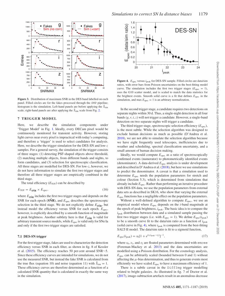
The impact of the uncertainty corrections is shown in Fig. 3,which compares the maximum SNR distribution in each band forfakes and the simulation. Compared to simulations with no correc-tion, simulations with corrections show much better agreement withthe fakes.

While equation (14) describes the simulated correction, there isan analogous correction for the data uncertainty produced by SMP:σSMP → σSMP × SSMP, where

SSMP( �O) = rms[(Ftrue − FSMP)/σ ′F ]fake

〈σSMP/σ′F 〉fake

. (15)

The observed scatter in the fakes is a common reference for boththe data and simulations, and therefore the numerator (equation 15)is the same as for the simulated correction (equation 14). Thedenominator, 〈σSMP/σ

′F 〉fake, specifies an average within each �O bin.

This SSMP correction is applied to the data uncertainties, includingfakes, while Ssim is applied to the simulated noise and uncertainty.More details of SSMP are given in Brout et al. (2018a).

MNRAS 485, 1171–1187 (2019)

Dow


ic.oup.com/m


H-U

SP user on 21 Decem

ber 2020


Figure 3. Distribution of maximum SNR in the DES band labelled on eachpanel. Filled circles are for the fakes processed through the SMP pipeline;histogram is the simulation. Left-hand panels are before applying the Ssim

scale; right-hand panels are after applying the Ssim scale from Fig. 2.

7 TR I G G E R MO D E L

Here, we describe the simulation components under‘Trigger Model’ in Fig. 1. Ideally, every DECam pixel would becontinuously monitored for transient activity. However, storinglight curves near every pixel is impractical with today’s computing,and therefore a ‘trigger’ is used to select candidates for analysis.Here, we describe the trigger simulation for the DES-SN and low-zsamples. For a general survey, the simulation of the trigger consistsof three stages: (1) detecting PSF-shaped objects above threshold,(2) matching multiple objects, from different bands and nights, toform candidates, and (3) selection for spectroscopic classification.All three stages are modelled for DES-SN. For low-z, however, wedo not have information to simulate the first two trigger stages andtherefore all three trigger stages are empirically combined in thethird stage.

The total efficiency (ETOT) can be described by

ETOT = E �SNR × Espec, (16)

where E �SNR includes the first two trigger stages and depends on theSNR for each epoch ( �SNR), and Espec describes the spectroscopicselection in the third stage. We do not explicitly define E �SNR, butinstead model the efficiency versus SNR for each epoch. Espec,however, is explicitly described by a smooth function of magnitudeat peak brightness. Another subtlety here is that E �SNR is valid forarbitrary transient source models, while Espec is valid only for SNe Iaand only if the first two trigger stages are satisfied.

7.1 DES-SN trigger

For the first trigger stage, fakes are used to characterize the detectionefficiency versus SNR in each filter, as shown in fig. 8 of Kessleret al. (2015). The efficiency reaches 50 per cent around SNR∼5.Since these efficiency curves are intended for simulations, we do notuse the measured SNR, but instead the fake SNR is calculated fromthe true flux (equation 10) and noise (equation 11) with Ssim = 1.These efficiency curves are therefore determined as a function of acalculated SNR quantity that is calculated in exactly the same wayin the simulation.

Figure 4. Espec versus ipeak for DES-SN sample. Filled circles are data/simratios, with error bars from Poisson uncertainties on the best-fitting modelcurve. The simulation includes the first two trigger stages (Espec = 1),uses the G10 scatter model, and is scaled to match the data statistics forthe brightest events. Smooth solid curve is a fit that defines Espec in thesimulation, and max Espec = 1 is an arbitrary normalization.

In the second trigger stage, a candidate requires two detections onseparate nights within 30 d. Thus, a single-night detection in all fourbands (g, r, i, z) will not trigger a candidate. However, a single-banddetection on two separate nights will trigger a candidate.

The third trigger stage, spectroscopic selection efficiency (Espec),is the most subtle. While the selection algorithm was designed toexclude human decisions as much as possible (D’Andrea et al.2018), we are not able to simulate the selection algorithm becausewe have eight frequently used telescopes, inefficiencies due toweather and scheduling, spectral classification uncertainty, and asmall amount of human decision making.

Ideally, we would compute Espec as a ratio of spectroscopicallyconfirmed events (numerator) to photometrically identified events(denominator). A data-derived Espec analysis is under developmentand described in D’Andrea et al. (2018), but here we use simulationsto predict the denominator. A caveat is that a simulation used todetermine Espec needs the population parameters for stretch andcolour (Section 5.3), which is determined from simulations thatalready include Espec. Rather than performing an iterative procedurewith DES-SN data, we use the population parameters from externaldata sets as described in SK16, who show that varying the externalEspec functions has a negligible effect on the population parameters.

Without a well-defined algorithm to compute Espec, we use anempirical model where Espec depends on the i-band magnitude atthe epoch of peak brightness, ipeak. The basic idea is to compare theipeak distribution between data and a simulated sample passing thefirst two trigger stages (i.e. with Espec = 1). We define Espec(ipeak)to be a smooth curve fit to the data/sim ratio as a function of ipeak

(solid curve in Fig. 4), where ipeak is computed from the best-fittingSALT-II model. The data/sim ratio is fit to a sigmoid function,

Espec(ipeak) = s0[1 + e(s1ipeak−s2)]−1, (17)

where s0, s1, and s2 are floated parameters determined with emcee(Foreman-Mackey et al. 2013) and the data uncertainties aremodelled using a Poisson distribution. For the cosmology analysis,Espec can be arbitrarily scaled (bounded between 0 and 1) withoutaffecting the μ-bias determination, and thus to generate events mostefficiently we have scaled Espec to have a maximum efficiency of 1.

There is a subtle caveat in the DiffImg trigger modellingrelated to bright galaxies. As illustrated in fig. 7 of Doctor et al.(2017), image-subtraction artefacts result in an anomalous decrease

MNRAS 485, 1171–1187 (2019)

Dow


ic.oup.com/m


H-U

SP user on 21 Decem

ber 2020


Figure 5. Espec versus Bpeak for each low-z sample. Filled circles are thedata/sim ratio with Espec = 1 in the simulation. Smooth curve is a fit thatdefines Espec in the simulation.

in detection efficiency as the local surface brightness increases.Here, the term ‘anomalous’ indicates an efficiency loss that is muchgreater than expected from the increased Poisson noise from thehost galaxy. While Fig. 2 shows how the SNANA simulation modelsanomalous scatter, the simulation does not model the anomalousdetection inefficiency. Studies with fakes have shown that thisbright-galaxy anomaly does not reduce the trigger efficiency fornearby SNe Ia on bright galaxies. The reason is that there are a fewdozen opportunities to acquire detections, and it is very unlikely tofail the two-detection trigger requirement.

7.2 Low-z trigger

As explained in Betoule et al. (2014) and Scolnic et al. (2014a),there is evidence that the low-z search is magnitude limited becauseof the decreasing number of events with redshift, and because higherredshift events are bluer. On the other hand, many low-z searchestarget a specific list of galaxies, suggesting a volume-limited sample.We therefore simulate both assumptions for evaluating systematicuncertainties.

For the magnitude-limited assumption, we incorporate all triggerstages into a single Espec function of B-band magnitude at the timeof peak brightness (Bpeak). Following the recipe for the DES-SNsimulation, we simulate a low-z sample with E �SNR = 1 and defineEspec to be the data/sim ratio versus Bpeak (Fig. 5). The fitted Bpeak

function is a one-sided Gaussian as described in appendix C ofScolnic et al. (2018a). Describing Espec as a function of V or R bandalso works well, so the choice of B band is arbitrary.

For the volume-limited assumption, which is used as a systematicuncertainty in Brout et al. (2018b), we set ETOT = 1 and interpret theredshift evolution of stretch and colour to be astrophysical effectsinstead of artifacts from Malmquist bias. To match the low-z data,the low-z simulation is tuned using redshift-dependent stretch andcolour populations: x1 → x1 + 25z and c → c − 1z. There is nophysical motivation for this redshift dependence, and therefore thisis a conservative assumption for the systematic uncertainty.

8 C O M PA R I N G DATA A N D S I M U L AT I O N S

Here, we qualitatively validate the simulations by comparingsimulated distributions with data. While we do not quantify thedata-simulation agreement here (e.g. via χ2), such quantitativecomparisons are used to assess systematic uncertainties in Broutet al. (2018b). To limit statistical uncertainties in these comparisons,very large simulations are generated and the distributions are scaledto match the statistics of the data. Recall that the tuned distributions

are Espec(ipeak) and the populations for stretch and colour; all otherinputs to the simulation are from measurements.

We apply light-curve fitting and selection requirements (cuts)that depend on SALT-II fitted parameters, SNR, and light-curvesampling (section 3.5 of Brout et al. 2018b). After applying thesecuts, data/simulation comparisons for DES-SN are shown in Fig. 6.The ipeak distribution for data and simulation are guaranteed to matchbecause of the method for determining Espec in Section 7.1. Theredshift agreement is not enforced, but is still excellent. The next twodistributions, E(B − V) and maximum gap between observations,are also in excellent agreement, and this agreement validates thechoice of random sky locations in the cadence library. The doublepeak structure of E(B − V) is from the large sky separations betweengroups of fields.

The middle column of Fig. 6 compares the maximum SNR ineach band, and these are the most difficult distributions to predictwith the simulation. The comparisons look good, except for a slightexcess in the simulation for SNR > 100. The right column of Fig. 6compares the local surface brightness mag in each band. There isgood agreement in all bands for SB < 24. For fainter hosts beyondthe detection limit the agreement is much poorer, and is likely dueto Malmquist bias for the limited co-add depth used in this analysis.Note that the poor agreement for faint hosts results in relativelysmall Ssim errors because Ssim → 1 (equation 11 and Fig. 2) as theunderlying host becomes more faint, and therefore, the range ofpossible Ssim corrections is smaller.

Fig. 7 shows data/simulation comparisons for the low-z sample.The Bpeak distributions are forced to match because of the methodfor determining Espec. The comparisons for redshift, E(B − V) andminimum Trest show excellent agreement. The comparisons formaximum gap between observations (rest-frame) and maximumB-band SNR indicate a slight discrepancy. The SNR agreement ispoorer compared to DES-SN because we do not have the observationinformation for the low-z sample, and thus rely on approximations(Section 6.1.1) to compute the noise in equation (11).

We have implemented SALT-II light-curve fits on the simulations,and fig. 7 of Brout et al. (2018b) shows data/simulation comparisonsfor the SALT-II parameters (mB, x1, c) and their uncertainties. Theexcellent agreement in these distributions adds confidence in ourμ-bias predictions.

9 D I S TA N C E M O D U L U S B I A S V E R S U SREDSHIFT

In one of our DES-SN3YR cosmology analyses (Brout et al. 2018b),we use the BBC method (Kessler & Scolnic 2017) in which μ-biasis characterized as a 5D function of {z, x1, c, α, β}. The first threeparameters are observed, and {α, β} are determined from the BBCfit. Here, we illustrate μ-bias as a function of redshift for a variety ofsub-samples, and also compare μ-bias for the two intrinsic scattermodels (G10,C11) from Section 5.2. It is important to note thatμ-bias is not a correction for the SN magnitude, but is a correctionfor fitted light-curve parameters (describing the stretch, colour andbrightness) along with a correction for the impact of intrinsic scatterin which brighter events are preferentially selected in a magnitude-limited survey.

The true distance modulus is defined as μtrue, and the mea-sured distance modulus (μ) is determined in the analysis fromTripp (1998),

μ = −2.5 log(x0) + αx1 − βc + M, (18)

MNRAS 485, 1171–1187 (2019)

Dow


ic.oup.com/m


H-U

SP user on 21 Decem

ber 2020


Figure 6. Comparison of data (black dots) and simulation with G10 scatter model (red histogram) for distributions in the DES-SN sample, where the simulationis scaled to have the same number of events as the data. Left column shows ipeak, CMB redshift, Galactic extinction, and maximum gap between observations(rest frame). Middle column shows log of maximum SNR in each band. Right column shows local surface mag in each band.

Figure 7. Data/simulation comparisons for distributions in the low-z sam-ple, using the G10 intrinsic scatter model and magnitude-limited selectionmodel.

where {x0, x1, c} are fitted SALT-II light-curve parameters, α

and β are the standardization parameters, and M is an offset sothat μ = μtrue when the true values of {x0, x1, c}true are used inequation (18). The distance modulus bias is defined as μ-bias ≡μ − μtrue. The BBC method applies a μ-bias correction for eachevent and determines the following parameters in a fit to the entiresample: α, β,M, and a weighted-average bias-corrected distancemodulus in discrete redshift bins.

We implement the BBC procedure on a simulated DES-SN3YRdata sample with 3 × 104 events after applying the cuts fromSection 8. The μ-bias thus has contributions from the DiffImgtrigger, spectroscopic selection, and analysis cuts. We use a large‘bias-correction’ sample with 1.3 × 106 events after the same cuts.Samples are generated with both the G10 and C11 intrinsic scatter

Figure 8. For the magnitude-limited low-z simulation, μ-bias variance-weighted average versus redshift for all events satisfying selection require-ments from Brout et al. (2018b) (left-hand panel), blue events with fittedc < −0.06 (middle panel), and red events with fitted c > 0.06 (right-handpanel). Filled circles are with simulations using the G10 intrinsic scattermodel; open circles are for the C11 model.

model, and the bias-correction sample with the correct intrinsicscatter model is used on the data; the effect of using the incorrectmodel is discussed in Brout et al. (2018b).

To account for a μ-bias dependence on α and β, we generate thebias-correction sample on a 2 × 2 grid of α × β and use this gridfor interpolation within the BBC fit. The grid values are α = {0.10,0.24}, βG10 = {2.7, 3.5}, and βC11 = {3.3, 4.3}.

The BBC-fitted values of α and β are un-biased withintheir 5 per cent statistical uncertainties, and fitting with optionalz-dependent slope parameters, dα/dz and dβ/dz are both consistentwith zero. M does not contribute to μ-bias and therefore the μ-biasis caused by the fitted light-curve parameters {x0, x1, c}. The μ-biasversus redshift from the BBC fit is shown in Figs 8 and 9 for the low-z and DES-SN samples, respectively. The filled circles correspondto the G10 intrinsic scatter model, and open circles correspond toC11.

MNRAS 485, 1171–1187 (2019)

Dow


ic.oup.com/m


H-U

SP user on 21 Decem

ber 2020


Figure 9. Same as Fig. 8, but for DES-SN.

Figure 10. For the DES-SN sample, left-hand panel shows μ-bias differ-ence versus redshift between α = 0.10 and α = 0.24. Right-hand panelshows μ-bias difference between different β values: {2.7, 3.3} for G10intrinsic scatter model (filled circles), and {3.3, 4.3} for C11 (open circles).

The average μ-bias (left-hand panels) is zero at the lower endof the redshift range. At higher redshifts, μ-bias depends on theintrinsic scatter model, reaching ∼0.05 mag at the high-redshiftrange. The middle and right panels of Figs 8 and 9 show thatμ-bias is much larger within restricted colour ranges, reaching upto 0.4 mag for the reddest (c > 0.06) events. All panels show a μ-biasdifference between the G10 and C11 models, and this difference islargely due to the different parent colour populations (Scolnic et al.2014b): the C11 colour population has a sharp cut-off on the blueside, while the G10 population has a tail extending bluer than inthe C11 model. These μ-bias differences, along with differences infitted α and β, are incorporated into the systematic uncertainty inBrout et al. (2018b).

The large μ-bias for red events at higher redshift is because mostof these events are intrinsically blue, which are bright enough tobe detected, but have poorly measured colours. Intrinsically redevents are fainter and thus tend to be excluded at higher redshifts.To illustrate the size of the colour uncertainties for the DES-SNsample, we computed the rms on measured colour minus true colour,rms(c), and the rms of the true colour population, rms(ctrue). Theratio is rms(c)/rms(ctrue) ∼ 0.5. Therefore, the typical differencebetween measured and true colour is 50 per cent of the size ofthe intrinsic colour distribution. For redshifts z > 0.5, this ratioincreases to 0.7. A similar exercise with the stretch parameter resultsin similar ratios.

As described in Section 5.3, a new feature in the BBC method isto account for the μ-bias dependence on {α, β}. This dependence isshown in Fig. 10 for DES-SN. Comparing simulations for α = 0.10

Figure 11. For the simulated DES-SN sample, (a) shows μ-bias versusredshift for light-curve fits that float x0 only, while fixing stretch and colourto their true values; (b) shows μ-bias versus redshift for nominal light-curvefits. Dashed line is for the ideal simulation defined as having no intrinsicscatter; solid line uses G10 intrinsic scatter model.

and α = 0.24 (nominal α � 0.15), the μ-bias difference reaches0.03 mag at high redshift, and is similar for the two intrinsic scattermodels (G10 and C11). The right-hand panel in Fig. 10 shows theμ-bias difference with β values differing by ∼1; the maximum μ-bias difference is 0.01 mag, and is similar for both intrinsic scattermodels.

We end this section by illustrating the contributions to μ-bias forred events (c > 0.06) in the right-hand panel of Fig. 9, where μ-bias reaches ∼0.4 mag at the highest redshifts. While high-redshiftbias is often associated with Malmquist bias, we show that μ-biasis primarily associated with intrinsic scatter and light-curve fitting.We begin with an ideal DES-SN simulation that has no intrinsicscatter, and perform light-curve fits in which only the amplitudex0 is floated while stretch and colour (x1, c) are assumed to beperfectly known. Defining m0 = −2.5log (x0), μ-bias, and m0-biasare the same. The resulting μ-bias is shown by the dashed curvein Fig. 11(a); this bias is only ∼0.01 mag, a very small fraction ofthe μ-bias in Fig. 9. While there may be selection bias in the twodetections contributing to the trigger (Section 7), the remaining fewdozen epochs are not biased, and thus the majority of observationsused to measure x0 are un-biased.

The solid curve in Fig. 11(a) shows μ-bias with the G10 intrinsicscatter model, and still fitting only for x0. In this case, μ-biasincreases considerably to about 0.1 mag at the highest redshift,and is a result of the strong brightness correlations among epochsand passbands. While the true intrinsic scatter variations average tozero, magnitude-limited observations preferentially select positivebrightness fluctuations, which lead to non-zero μ-bias.

Fig. 11(b) shows the same simulations, but with light-curve fitsthat float all three parameters (x0, x1, c). Compared with Fig. 11(a),the μ-bias is much larger, mainly because of the bias in fitted colour.Although this μ-bias test is shown only for the red events in Fig. 9,similar trends exist in all colour ranges.

The statistical uncertainties on these μ-bias corrections arenegligible. Systematic uncertainties in Brout et al. (2018b) are thusdetermined from changing input assumptions such as the colour andstretch populations, model of intrinsic scatter, and the value of theflux-uncertainty scale, Ssim.

1 0 C O N C L U S I O N

The SNANA simulation program has been under active developmentfor a decade, and has been used in several cosmology analyses

MNRAS 485, 1171–1187 (2019)

Dow


ic.oup.com/m


H-U

SP user on 21 Decem

ber 2020


to accurately simulate SN Ia light curves and determine biascorrections for the distance moduli. This work focuses on simulatedbias corrections for the DES-SN3YR sample, which combinesspectroscopically confirmed SNe Ia from DES-SN and low-redshiftsamples. Files used to make these corrections are available athttps://des.ncsa.illinois.edu/releases/sn.

The DES-SN simulation includes three categories of detailedmodelling: (1) source model including the rest-frame SN Ia SED,cosmological dimming, weak lensing, peculiar velocity, and Galac-tic extinction; (2) noise model accounting for observation properties(PSF, sky noise, zero-point), host galaxy, and information derivedfrom 10 000 fake SN light curves overlaid on images and run throughour image-processing pipelines; (3) trigger model of single-visitdetections, candidate logic, and spectroscopic selection efficiency.The low-z sample, however, does not include observation properties,and thus approximations are used to simulate this sample. Thequality of the simulation is illustrated by predicting observeddistributions (Figs 6 and 7), and bias corrections on the distancemoduli are shown in Figs 8 and 9.

The reliability of the bias corrections is only as good as theunderlying assumptions in the simulation. To properly propagatebias correction uncertainties into systematic uncertainties on cos-mological parameters, Brout et al. (2018a) evaluate uncertaintiesfor each of the three modelling categories above (source, noise,trigger). In addition to explicit assumptions such as those associatedwith the SALT-II model, one should always be aware of the implicitassumptions such as simulating SN properties (e.g. α, β) that areindependent of redshift and host-galaxy properties.

The simulations presented here are used to correct SN Ia distancebiases in the DES-SN3YR sample (Brout et al. 2018b), andthese bias-corrected distances are used to measure cosmologicalparameters (DES Collaboration et al. 2018). These simulations alsoserve as a starting point for the analysis of the full DES 5-yearphotometrically classified sample, which will be significantly largerthan the DES-SN3YR sample.

AC K N OW L E D G E M E N T S

This work was supported in part by the Kavli Institute for Cos-mological Physics at the University of Chicago through grant NSFPHY-1125897 and an endowment from the Kavli Foundation and itsfounder Fred Kavli. This work was completed in part with resourcesprovided by the University of Chicago Research Computing Center.RK is supported by DOE grant DE-AC02-76CH03000. DS issupported by NASA through Hubble Fellowship grant HST-HF2-51383.001 awarded by the Space Telescope Science Institute, whichis operated by the Association of Universities for Research inAstronomy, Inc., for NASA, under contract NAS 5-26555. TheU.Penn group was supported by DOE grant DE-FOA-0001358and NSF grant AST-1517742. AVF’s group at U.C. Berkeley isgrateful for financial assistance from NSF grant AST-1211916, theChristopher R. Redlich Fund, the TABASGO Foundation, and theMiller Institute for Basic Research in Science.

Funding for the DES Projects has been provided by the U.S.Department of Energy, the U.S. National Science Foundation,the Ministry of Science and Education of Spain, the Scienceand Technology Facilities Council of the United Kingdom, theHigher Education Funding Council for England, the National Centerfor Supercomputing Applications at the University of Illinois atUrbana-Champaign, the Kavli Institute of Cosmological Physicsat the University of Chicago, the Center for Cosmology andAstro-Particle Physics at the Ohio State University, the Mitchell

Institute for Fundamental Physics and Astronomy at Texas A&MUniversity, Financiadora de Estudos e Projetos, Fundacao CarlosChagas Filho de Amparo a Pesquisa do Estado do Rio de Janeiro,Conselho Nacional de Desenvolvimento Cientıfico e Tecnologicoand the Ministerio da Ciencia, Tecnologia e Inovacao, the DeutscheForschungsgemeinschaft and the Collaborating Institutions in theDark Energy Survey.

The Collaborating Institutions are Argonne National Laboratory,the University of California at Santa Cruz, the University ofCambridge, Centro de Investigaciones Energeticas, Medioambien-tales y Tecnologicas-Madrid, the University of Chicago, Univer-sity College London, the DES-Brazil Consortium, the Universityof Edinburgh, the Eidgenossische Technische Hochschule (ETH)Zurich, Fermi National Accelerator Laboratory, the University ofIllinois at Urbana-Champaign, the Institut de Ciencies de l’Espai(IEEC/CSIC), the Institut de Fısica d’Altes Energies, LawrenceBerkeley National Laboratory, the Ludwig-Maximilians UniversitatMunchen and the associated Excellence Cluster Universe, theUniversity of Michigan, the National Optical Astronomy Obser-vatory, the University of Nottingham, The Ohio State University,the University of Pennsylvania, the University of Portsmouth,SLAC National Accelerator Laboratory, Stanford University, theUniversity of Sussex, Texas A&M University, and the OzDESMembership Consortium.

Based in part on observations at Cerro Tololo Inter-AmericanObservatory, National Optical Astronomy Observatory, which isoperated by the Association of Universities for Research in As-tronomy (AURA) under a cooperative agreement with the NationalScience Foundation.

The DES data management system is supported by the Na-tional Science Foundation under Grant Numbers AST-1138766and AST-1536171. The DES participants from Spanish institu-tions are partially supported by MINECO under grants AYA2015-71825, ESP2015-66861, FPA2015-68048, SEV-2016-0588, SEV-2016-0597, and MDM-2015-0509, some of which include ERDFfunds from the European Union. IFAE is partially funded by theCERCA programme of the Generalitat de Catalunya. Researchleading to these results has received funding from the EuropeanResearch Council under the European Union’s Seventh Frame-work Program (FP7/2007-2013) including ERC grant agreements240672, 291329, and 306478. We acknowledge support from theAustralian Research Council Centre of Excellence for All-skyAstrophysics (CAASTRO), through project number CE110001020,and the Brazilian Instituto Nacional de Ciencia e Tecnologia (INCT)e-Universe (CNPq grant 465376/2014-2).

This manuscript has been authored by Fermi Research Alliance,LLC under Contract No. DE-AC02-07CH11359 with the USDepartment of Energy, Office of Science, Office of High EnergyPhysics. The United States Government retains and the publisher, byaccepting the article for publication, acknowledges that the UnitedStates Government retains a non-exclusive, paid-up, irrevocable,world-wide license to publish or reproduce the published formof this manuscript, or allow others to do so, for United StatesGovernment purposes.

REFERENCES

Astier P. et al., 2006, A&A, 447, 31Barnes J., Kasen D., 2013, ApJ, 775, 18Bernstein J. P. et al., 2012, ApJ, 753, 152Betoule M. et al., 2014, A&A, 568, A22Brout D. et al., 2018a, ApJ, preprint (arXiv:1811.02378)

MNRAS 485, 1171–1187 (2019)

Dow


ic.oup.com/m


H-U

SP user on 21 Decem

ber 2020

https://des.ncsa.illinois.edu/releases/sn

http://dx.doi.org/10.1088/0004-637X/775/1/18

http://dx.doi.org/10.1088/0004-637X/753/2/152

http://arxiv.org/abs/1811.02378


Brout D. et al., 2018b, ApJ, preprint (arXiv:1811.02377)Burns C. R. et al., 2011, AJ, 141, 19Carretero J., Castander F. J., Gaztanaga E., Crocce M., Fosalba P., 2015,

MNRAS, 447, 646Chotard N. et al., 2011, A&A, 529, L4Conley A. et al., 2011, ApJS, 192, 1Contreras C. et al., 2010, AJ, 139, 519Crocce M., Castander F. J., Gaztanaga E., Fosalba P., Carretero J., 2015,

MNRAS, 453, 1513D’Andrea D. et al., 2018, preprint (arXiv:1811.09565)Davis T. M., Hui L., Frieman J. A. et al., 2011, ApJ, 741, 67Delgado F. et al., 2014, in Proc. SPIE Conf. Ser. Vol. 9150, Modeling,

Systems Engineering, and Project Management for Astronomy VI. SPIE,Bellingham, p. 915015

DES Collaboration et al., 2018, preprint (arXiv:1811:02374)Diehl H. T. et al., 2016, in Proc. SPIE Conf. Ser. Vol. 9910, Observatory

Operations: Strategies, Processes, and Systems VI. SPIE, Bellingham,p. 99101D

Diemer B., Kessler R., Graziani C., Jordan G. C., IV, Lamb D. Q., LongM., van Rossum D. R., 2013, ApJ, 773, 119

Doctor Z. et al., 2017, ApJ, 837, 57Fitzpatrick E. L., 1999, PASP, 111, 63Flaugher B. et al., 2015, AJ, 150, 150Folatelli G. et al., 2010, AJ, 139, 120Foreman-Mackey D., Hogg D. W., Lang D., Goodman J., 2013, PASP, 125,

306Frieman J. A. et al., 2008, AJ, 135, 338Ganeshalingam M., Li W., Filippenko A. V., 2013, MNRAS, 433, 2240Goldstein D. A., D’Andrea C. B., Fischer J. A. et al., 2015, AJ, 150, 82Gupta R. R. et al., 2016, AJ, 152, 154Guy J. et al., 2010, A&A, 523, A7Hicken M. et al., 2009, ApJ, 700, 331Hicken M. et al., 2012, ApJS, 200, 12Hounsell R. et al., 2018, ApJ, 867, 23Hsiao E. Y., Conley A., Howell D. A., Sullivan M., Pritchet C. J., Carlberg

R. G., Nugent P. E., Phillips M. M., 2007, ApJ, 663, 1187Jha S., Riess A. G., Kirshner R. P., 2007, ApJ, 659, 122Jones D. O. et al., 2017, ApJ, 843, 6Jones D. O. et al., 2018, ApJ, 857, 27Kaiser N. et al., 2002, in Tyson J. A., Wolff S., eds, Proc. SPIE Conf. Ser.

Vol. 4836, Survey and Other Telescope Technologies and Discoveries.SPIE, Bellingham, p. 154

Kessler R. et al., 2009a, ApJS, 185, 32Kessler R. et al., 2009b, PASP, 121, 1028Kessler R. et al., 2010a, PASP, 122, 1415Kessler R. et al., 2010b, ApJ, 717, 40Kessler R. et al., 2013, ApJ, 764, 48Kessler R. et al., 2015, AJ, 150, 172Kessler R., Scolnic D., 2017, ApJ, 836, 56LSST Science Collaboration et al., 2009, preprint (arXiv:0912.0201)Madau P., Dickinson M., 2014, ARA&A, 52, 415Mannucci F., Della Valle M., Panagia N., 2006, MNRAS, 370, 773Mosher J. et al., 2014, ApJ, 793, 16Perlmutter S. et al., 1999, ApJ, 517, 565Perrett K. et al., 2012, AJ, 144, 59Rest A. et al., 2014, ApJ, 795, 44Riess A. G. et al., 1998, AJ, 116, 1009Rodney S. A. et al., 2012, ApJ, 746, 5Rubin D. et al., 2015, ApJ, 813, 137Sako M. et al., 2018, PASP, 130, 064002Scannapieco E., Bildsten L., 2005, ApJ, 629, L85Schlafly E. F., Finkbeiner D. P., 2011, ApJ, 737, 103Schlegel D. J., Finkbeiner D. P., Davis M., 1998, ApJ, 500, 525Scolnic D., Kessler R., 2016, ApJ, 822, L35 (SK16)Scolnic D.et al., 2014a, ApJ, 795, 45Scolnic D. M., Riess A. G., Foley R. J., Rest A., Rodney S. A., Brout D. J.,

Jones D. O., 2014b, ApJ, 780, 37Scolnic D. M. et al., 2018a, ApJ, 859, 28

Scolnic D. et al., 2018b, ApJ, 852, L3Singer L. P. et al., 2016a, ApJ, 829, L15Singer L. P. et al., 2016b, ApJS, 226, 10Soares-Santos M. et al., 2016, ApJ, 823, L33Strolger L.-G. et al., 2015, ApJ, 813, 93Tripp R., 1998, A&A, 331, 815

APPENDI X: ADDI TI ONA L SI MULATI ONF E ATU R E S FO R F U T U R E A NA LY S I S

The focus of this work has been on simulating bias correctionsand validation samples for the DES-SN3YR SN Ia cosmologyanalysis. Here, we describe additional features of the SNANA

simulation that have been developed for future work, but arebeyond the current scope of the DES-SN3YR analysis. This futurework includes extending the cosmology analysis to photometricallyidentified SNe Ia, more detailed systematics studies, determiningthe efficiency for Bayesian cosmology fitting methods (e.g. Rubinet al. 2015), determining the efficiency for SN rate studies, andoptimizing future surveys. We end with a summary of missingfeatures that would be useful to add for future analysis work.

A1 SED time-series

The SALT-II light-curve model, which is designed for SN Iacosmology analyses, is a rather complex semi-analytical model.Most transient models, however, are much simpler. In additionto specialized SN Ia models,10 the SNANA simulation workswith arbitrary collections of SED time-series. Each event can begenerated from a random SED time-series, or computed fromparametric interpolation. For example, suppose a set of Np pa-rameters, �P = {p1, p2, ...pNp

}, describes each SED time-series.Each parameter (pi) can be drawn from a Gaussian distribution(or asymmetric Gaussian) and a full covariance matrix to inducecorrelations. The SEDs on the parameter grid are interpolated to thegenerated �P .

Examples include CC simulations to model contamination inphotometrically identified SN Ia samples (Kessler et al. 2010a;Rodney et al. 2012; Jones et al. 2017; Kessler & Scolnic 2017), andsimulating Kilonovae (Barnes & Kasen 2013) to model the searchefficiency (Soares-Santos et al. 2016; Doctor et al. 2017), and topredict discovery rates (Scolnic et al. 2018).

An SED time-series can also be useful for modelling SNe Ia.Examples include systematic studies on training the SALT-II modelwith simulated spectra (Hsiao et al. 2007; Mosher et al. 2014),and simulating spectra from SN Ia explosion models (Diemer et al.2013; Kessler et al. 2013).

A2 Light-curve library for galactic transients

Galactic transients can potentially contribute contamination ina photometrically identified SN Ia sample. To model galactictransients, the simulation reads a pre-computed ‘light-curve library’of transient magnitudes versus time. The light curves can be recur-ring or non-recurring. For recurring and long-lived non-recurringtransients, the library specifies source magnitudes at epochs to useas templates for image-subtraction, and the simulation accounts forsource signal in the templates. The subtracted fluxes can therefore be

10SN Ia models in SNANA include SALT-II (Guy et al. 2010), MLCS2k2(Jha, Riess & Kirshner 2007), and SNOOPY (Burns et al. 2011).

MNRAS 485, 1171–1187 (2019)

Dow


ic.oup.com/m


H-U

SP user on 21 Decem

ber 2020


http://dx.doi.org/10.1088/0004-6256/141/1/19

http://dx.doi.org/10.1093/mnras/stu2402

http://dx.doi.org/10.1088/0067-0049/192/1/1

http://dx.doi.org/10.1088/0004-6256/139/2/519

http://dx.doi.org/10.1093/mnras/stv1708


http://dx.doi.org/10.1088/0004-637X/741/1/67

http://arxiv.org/abs/1811:02374

http://dx.doi.org/10.1088/0004-637X/773/2/119

http://dx.doi.org/10.3847/1538-4357/aa5d09

http://dx.doi.org/10.1086/316293

http://dx.doi.org/10.1088/0004-6256/150/5/150

http://dx.doi.org/10.1088/0004-6256/139/1/120

http://dx.doi.org/10.1086/670067

http://dx.doi.org/10.1088/0004-6256/135/1/338

http://dx.doi.org/10.1093/mnras/stt893

http://dx.doi.org/10.1088/0004-6256/150/3/82

http://dx.doi.org/10.3847/0004-6256/152/6/154

http://dx.doi.org/10.1088/0004-637X/700/1/331

http://dx.doi.org/10.1088/0067-0049/200/2/12

http://dx.doi.org/10.3847/1538-4357/aac08b

http://dx.doi.org/10.1086/518232

http://dx.doi.org/10.1086/512054

http://dx.doi.org/10.3847/1538-4357/aab6b1

http://dx.doi.org/10.1088/0067-0049/185/1/32

http://dx.doi.org/10.1086/605984

http://dx.doi.org/10.1086/657607

http://dx.doi.org/10.1088/0004-637X/717/1/40

http://dx.doi.org/10.1088/0004-637X/764/1/48

http://dx.doi.org/10.1088/0004-6256/150/6/172

http://dx.doi.org/10.3847/1538-4357/836/1/56


http://dx.doi.org/10.1111/j.1365-2966.2006.10501.x

http://dx.doi.org/10.1088/0004-637X/793/1/16

http://dx.doi.org/10.1086/307221

http://dx.doi.org/10.1088/0004-6256/144/2/59

http://dx.doi.org/10.1088/0004-637X/795/1/44

http://dx.doi.org/10.1086/300499

http://dx.doi.org/10.1088/0004-637X/746/1/5

http://dx.doi.org/10.1088/0004-637X/813/2/137

http://dx.doi.org/10.1086/452632

http://dx.doi.org/10.1088/0004-637X/737/2/103

http://dx.doi.org/10.1086/305772

http://dx.doi.org/10.3847/2041-8205/822/2/L35

http://dx.doi.org/10.1088/0004-637X/795/1/45

http://dx.doi.org/10.1088/0004-637X/780/1/37

http://dx.doi.org/10.3847/1538-4357/aab9bb

http://dx.doi.org/10.3847/2041-8213/aa9d82

http://dx.doi.org/10.3847/2041-8205/829/1/L15

http://dx.doi.org/10.3847/0067-0049/226/1/10

http://dx.doi.org/10.3847/2041-8205/823/2/L33

http://dx.doi.org/10.1088/0004-637X/813/2/93


positive or negative. To detect negative fluxes with SNR < 0, thereis an option to define the detection efficiency as a function of |SNR|.Each library light curve is overlaid on the survey time-window, andoverlapping observations in the cadence library are converted intoa measured flux and uncertainty. Readers are cautioned that thismodel is relatively new, and has not yet been used in a publication.

A3 Characterization of detection efficiency

For the DES-SN3YR analysis, the DES detection efficiency wasadequately characterized as a function of SNR. In the next cos-mology analysis with a much larger photometric sample, we mayneed a more accurate description. In particular, we may need tocharacterize the efficiency of a machine learning (ML) requirementin DiffImg that was used to reject image-subtraction artefacts(Goldstein et al. 2015). The SNANA data file structure includesa ‘PHOTPROB’ entry for each epoch, which is intended to storeinformation such as an ML score. The simulation can generateML scores (between 0 and 1) based on an input probability mapthat depends on SNR and/or mSB. The input ML map should begenerated from fakes processed through the same pipeline as thedata. Since ML scores describe imaging data near the source, thesescores are likely to be correlated among different epochs. A reducedcorrelation (0 to 1) can be provided to introduce ML correlations.

While we have been characterizing anomalous effects as afunction of mSB, we have begun exploring the dependence on m− mSB, where m is the source magnitude. This source-to-galaxyflux ratio can be used to describe the detection efficiency or the MLmap.

A4 Characterization of flux-uncertainty scale

In Section 6.4, the flux-uncertainty scale, Ssim, was defined as afunction of 1 parameter: mSB. In future work, we plan to investigateif Ssim depends on other parameters. The additional Ssim-dependentparameters in the simulation are: (1) SNR, (2) PSF, (3) MJD, (4)sky noise, (5) zero-points, (6) galaxy magnitude, and (7) SN-hostseparation. Additional parameters, such as the source-to-galaxy fluxratio, can be added with minor code modifications.

A5 Rate models

The following rate models can be used in the SNANA simulation:

(i) R(z) = α(1 + z)β with user-specified α, β. Multiple R(z)functions can be defined, each in a different redshift range.

(ii) R(z) = A · ∫ z

∞ dz′SFR(z′) + B · SFR(z), where SFR is thestar formation rate, A is the amplitude of the delayed component,and B is the amplitude of the prompt component (Scannapieco &Bildsten 2005; Mannucci, Della Valle & Panagia 2006).

(iii) CC R(z) measured with HST (Strolger et al. 2015).(iv) Star formation R(z) from Madau & Dickinson (2014), where

user defines R(0).

A6 Redshift-dependent input parameters

Since redshift evolution is a concern in cosmology analyses, anysimulation-input parameter can be given a redshift dependence: P→ P + p1z + p2z

2 + p3z3, where P is a user-specified simulation

parameter and p1,2,3 are user-defined parameters. If a third-orderpolynomial is not adequate, the simulation can read an explicit P(z)map in arbitrary redshift bins.

A7 Population parametrization

The SALT-II colour and stretch populations are described by twoasymmetric Gaussian profiles. The probability for colour is definedas

P (c) ∝ exp[−(c − c)2/2σ 2+] (c ≥ c) (A1)

P (c) ∝ exp[−(c − c)2/2σ 2−] (c < c) (A2)

and similarly for P(x1). A second asymmetric Gaussian can beadded, as described in appendix C of Scolnic et al. (2018a) for thelow-z stretch distribution.

A8 Inhomogeneous distributions

The DES-SN3YR simulations assume an isotropic and homo-geneous universe on all distance scales because of the randomselection of sky coordinates in the observation library (Section 6.1)and the random generation of redshifts. Large-scale structure canbe incorporated, but requires an external simulation to generatethree-dimensional (RA, Dec., z) galaxy locations. For each suchgalaxy, the RA, Dec., and redshift are used to create an entry in theobservation library.

Another application is to simulate transients corresponding toa posterior from a gravitational wave event found by the LargeInterferometer Gravity Wave Observatory (LIGO; Singer et al.2016a,b). Drawing random events from the posterior described byRA, Dec., and distance, each event corresponds to an entry in theobservation library.

A9 Host-galaxy library features

A host-galaxy library (HOSTLIB) was defined in Section 6.2 tomodel additional Poisson noise and the local surface brightness.Additional HOSTLIB features include:

(i) mis-matched host redshift model for photometrically identi-fied sample (Jones et al. 2016),

(ii) a weight map to assign SN magnitude offsets based on host-galaxy mass, or other properties such as specific star formationrate,

(iii) photometric galaxy redshift (ZPHOT) and Gaussian uncer-tainty (ZPHOTERR), which must be computed externally frombroad-band filters,

(iv) brightness distribution described with arbitrary sum of Sersicprofiles, each with its own index,

(v) correlation of host and SN properties by including SALT-IIcolour and stretch for each HOSTLIB event.

A10 Generating spectra

Ideally, the modelling of spectroscopic selection would include ananalysis of simulated spectra, but instead we empirically modelthis efficiency as a function of peak magnitude. To begin the efforton modelling spectroscopic selection, the SNANA simulation wasenhanced to generate spectra for the WFIRST simulation studyin Hounsell et al. (2018). Spectra are characterized by their SNRversus wavelength. They can be generated at specific dates in theobservation library, or a random date can be selected in time-windows with respect to peak brightness. This time-window canbe specified in either the rest frame or observer frame, although the

MNRAS 485, 1171–1187 (2019)

Dow


ic.oup.com/m


H-U

SP user on 21 Decem

ber 2020


former is more difficult to carry out in practice. Spectral slices canalso be integrated and stored as broad-band fluxes.

Finally, a high-SNR (low-z) spectrum can be simulated atarbitrary redshift to examine the expected SNR degradation versusdistance.

A11 Missing features

We finish this section with a few features that are not included inthe simulation, but might be useful in future analyses:

(i) peculiar velocity covariances (currently all vpec are uncorre-lated),

(ii) galactic E(B − V) covariance (currently all extinctions areuncorrelated),

(iii) spectral PCA coefficients in the HOSTLIB to model hostcontamination in spectra,

(iv) probability distribution for host-galaxy photometric redshifts(instead of Gaussian-error approximation),

(v) anomalous detection inefficiency from bright galaxies,(vi) weak lensing magnification model (Section 5.4) accounting

for correlations between events with small angular separations.

1Department of Astronomy and Astrophysics, University of Chicago,Chicago, IL 60637, USA2Kavli Institute for Cosmological Physics, University of Chicago, Chicago,IL 60637, USA3Department of Physics and Astronomy, University of Pennsylvania,Philadelphia, PA 19104, USA4School of Mathematics and Physics, University of Queensland, Brisbane,QLD 4072, Australia5Lawrence Berkeley National Laboratory, 1 Cyclotron Road, Berkeley, CA94720, USA6The Research School of Astronomy and Astrophysics, Australian NationalUniversity, ACT 2601, Australia7Institute of Cosmology and Gravitation, University of Portsmouth,Portsmouth PO1 3FX, UK8ARC Centre of Excellence for All-sky Astrophysics (CAASTRO), Sydney,Australia9School of Physics and Astronomy, University of Southampton, SouthamptonSO17 1BJ, UK10University of Copenhagen, Dark Cosmology Centre, Juliane Maries Vej30, DK-2100 Copenhagen Ø, Denmark11Korea Astronomy and Space Science Institute, Yuseong-gu, Daejeon, 305-348, Korea12Harvard-Smithsonian Center for Astrophysics, 60 Garden Str, Cambridge,MA 02138, USA13INAF, Astrophysical Observatory of Turin, I-10025 Pino Torinese, Italy14Millennium Institute of Astrophysics and Department of Physics andAstronomy, Universidad Catolica de Chile, Santiago, Chile15South African Astronomical Observatory, PO Box 9, Observatory 7935,South Africa16Space Telescope Science Institute, 3700 San Martin Drive, Baltimore, MD21218, USA17Department of Astronomy, University of California, Berkeley, CA 94720-3411, USA18Miller Senior Fellow, Miller Institute for Basic Research in Science,University of California, Berkeley, CA 94720, USA19Santa Cruz Institute for Particle Physics, Santa Cruz, CA 95064, USA20Centre for Astrophysics & Supercomputing, Swinburne University ofTechnology, Victoria 3122, Australia21Department of Physics, University of Namibia, 340 Mandume NdemufayoAvenue, Pionierspark, Windhoek, Namibia22Harvard-Smithsonian Center for Astrophysics, 60 Garden Str, Cambridge,MA 02138, USA

23Gordon and Betty Moore Foundation, 1661 Page Mill Road, Palo Alto,CA 94304, USA24Sydney Institute for Astronomy, School of Physics, A28, The University ofSydney, NSW 2006, Australia25Institute of Astronomy and Kavli Institute for Cosmology, Madingley Road,Cambridge CB3 0HA, UK26National Center for Supercomputing Applications, 1205 West Clark St.,Urbana, IL 61801, USA27Institute of Astronomy, University of Cambridge, Madingley Road, Cam-bridge CB3 0HA, UK28Division of Theoretical Astronomy, National Astronomical Observatoryof Japan, 2-21-1 Osawa, Mitaka, Tokyo 181-8588, Japan29Institute of Astronomy and Astrophysics, Academia Sinica, Taipei 10617,Taiwan30Observatories of the Carnegie Institution for Science, 813 Santa BarbaraStr, Pasadena, CA 91101, USA31Cerro Tololo Inter-American Observatory, National Optical AstronomyObservatory, Casilla 603, La Serena, Chile32Fermi National Accelerator Laboratory, PO Box 500, Batavia, IL 60510,USA33Kavli Institute for Cosmology, University of Cambridge, Madingley Road,Cambridge CB3 0HA, UK34LSST, 933 North Cherry Avenue, Tucson, AZ 85721, USA35CNRS, UMR 7095, Institut d’Astrophysique de Paris, F-75014, Paris,France36Sorbonne Universites, UPMC Univ Paris 06, UMR 7095, Institutd’Astrophysique de Paris, F-75014 Paris, France37Department of Physics & Astronomy, University College London, GowerStreet, London WC1E 6BT, UK38Kavli Institute for Particle Astrophysics & Cosmology, PO Box 2450,Stanford University, Stanford, CA 94305, USA39SLAC National Accelerator Laboratory, Menlo Park, CA 94025,USA40Centro de Investigaciones Energeticas, Medioambientales y Tecnologicas(CIEMAT), Madrid, Spain41Laboratorio Interinstitucional de e-Astronomia - LIneA, Rua Gal. JoseCristino 77, Rio de Janeiro, RJ – 20921-400, Brazil42Department of Astronomy, University of Illinois at Urbana-Champaign,1002 W. Green Str, Urbana, IL 61801, USA43Institut de Fısica d’Altes Energies (IFAE), The Barcelona Institute ofScience and Technology, Campus UAB, E-08193 Bellaterra (Barcelona),Spain44Institut d’Estudis Espacials de Catalunya (IEEC), E-08034 Barcelona,Spain45Institute of Space Sciences (ICE, CSIC), Campus UAB, Carrer de CanMagrans, s/n, E-08193 Barcelona, Spain46Observatorio Nacional, Rua Gal. Jose Cristino 77, Rio de Janeiro, RJ –20921-400, Brazil47Department of Physics, IIT Hyderabad, Kandi, Telangana 502285, India48Department of Astronomy/Steward Observatory, 933 North Cherry Av-enue, Tucson, AZ 85721, USA49Jet Propulsion Laboratory, California Institute of Technology, 4800 OakGrove Dr., Pasadena, CA 91109, USA50Instituto de Fisica Teorica UAM/CSIC, Universidad Autonoma de Madrid,E-28049 Madrid, Spain51Department of Astronomy, University of Michigan, Ann Arbor, MI 48109,USA52Department of Physics, University of Michigan, Ann Arbor, MI 48109,USA53Department of Physics, ETH Zurich, Wolfgang-Pauli-Strasse 16, CH-8093Zurich, Switzerland54Center for Cosmology and Astro-Particle Physics, The Ohio State Uni-versity, Columbus, OH 43210, USA55Department of Physics, The Ohio State University, Columbus, OH 43210,USA56Harvard-Smithsonian Center for Astrophysics, Cambridge, MA 02138,USA

MNRAS 485, 1171–1187 (2019)

Dow


ic.oup.com/m


H-U

SP user on 21 Decem

ber 2020


57Australian Astronomical Optics, Macquarie University, North Ryde, NSW2113, Australia58Departamento de Fısica Matematica, Instituto de Fısica, Universidade deSao Paulo, CP 66318, Sao Paulo, SP, 05314-970, Brazil59George P. and Cynthia Woods Mitchell Institute for Fundamental Physicsand Astronomy, and Department of Physics and Astronomy, Texas A&MUniversity, College Station, TX 77843, USA60Department of Astronomy, The Ohio State University, Columbus, OH43210, USA61Institucio Catalana de Recerca i Estudis Avancats, E-08010 Barcelona,Spain

62Brandeis University, Physics Department, 415 South Str, Waltham, MA02453, USA63Instituto de Fısica Gleb Wataghin, Universidade Estadual de Campinas,13083-859, Campinas, SP, Brazil64Computer Science and Mathematics Division, Oak Ridge National Labo-ratory, Oak Ridge, TN 37831, USA

This paper has been typeset from a TEX/LATEX file prepared by the author.

MNRAS 485, 1171–1187 (2019)

Dow


ic.oup.com/m


H-U

SP user on 21 Decem

ber 2020

first cosmology results using type ia supernova from the

Documents