1

Fiscal Policy for Public Debt Stabilization in a Multiple Household

Dynamic General Equilibrium Model for Brazil

Octavio Augusto Fontes Tourinho

Fernando Moraes Carneiro⁑

ABSTRACT

This paper specifies an open economy dynamic applied general equilibrium model with government, public

debt and heterogeneous households. We calibrate the model for the Brazilian economy and use it to study

fiscal mix and public debt stabilization policies in the short and long term. Households are Ricardian or

non-Ricardian depending to their access to financial markets, and we find that the welfare impact on them

of the several fiscal policies can be quite different. Only two changes of fiscal mix imply gains for both,

and none of the debt consolidation policies are desirable for both. We claim that heterogeneity of

households may lead to a lack of agreement with regards to public debt consolidation, political conflict in

adoption of fiscal policies to control it, and chronic public debt accumulation.

Keywords: Fiscal Policy. Public Debt. Dynamic General Equilibrium. Growth Models. non-Ricardian

Households.

JEL: E62, H63, D58, O54

RESUMO

Este artigo apresenta um modelo de equilíbrio geral dinâmico com economia aberta, governo, dívida

pública e famílias heterogêneas. Nós calibramos o modelo para a economia brasileira e o utilizamos para

estudar os efeitos, no curto e longo prazo, de políticas que alterem parâmetros fiscais e estabilizem a dívida

pública. As famílias são Ricardianas ou não-Ricardianas, dependendo do acesso ao mercado financeiro, e

os resultados indicam que o impacto das diferentes estratégias de política fiscal sobre o bem-estar delas

pode ser bastante diferente. Apenas duas políticas que alteram os parâmetros fiscais implicam ganhos para

ambas, e nenhuma das políticas de consolidação da dívida é desejável para ambas. Este estudo conclui que

a heterogeneidade das famílias pode levar à falta de concordância em relação à consolidação da dívida

pública, ao conflito político na adoção de políticas fiscais para controlá-la e ao endividamento persistente.

Palavras-chave: Política Fiscal. Dívida Pública. Equilíbrio Geral Dinâmico. Modelos de Crescimento.

Famílias Não-Ricardianas.

JEL: E62, H63, D58, O54

Área 4 (ANPEC): Macroeconomia, Economia Monetária e Finanças.

UERJ - Universidade do Estado do Rio de Janeiro. E-mail: otourinho@uerj.br ⁑ UERJ – Universidade do Estado do Rio de Janeiro. E-mail: fm.carneiro@yahoo.com.br

2

1. Introduction

In the last 20 years fiscal policy has faced several challenges in many countries around the world.

In several cases public debt has increased significantly as a result of fiscal permissiveness in financing the

increasing cost and breadth of social security, expansion and creation of social programs, development of

large infrastructure projects, and of granting of subsidies, and of tax forfeiture.1 More recently, in many

countries it has further increased by the use of debt financed expansionary policies used in response to the

recessionary effects of the subprime crisis of 2008. The interest cost of the larger public debt has further

aggravated the fiscal imbalance.

Irrespective of its origin, the resulting disequilibrium has required the adoption of fiscal austerity

programs to control the growth of public indebtedness. These policies, however, have a high social cost in

the short and medium term, and their political acceptance is often complex, controversial and difficult. To

assist in their design and evaluation, studies have been undertaken in several countries to prospectively

assess their effectiveness, sustainability, and economic impact, especially on growth.2 The present study

aims to contribute to that literature, with special reference to Brazil.

The Brazilian fiscal problem is chronic, as shown by Giambiagi and Além (2016). The last five

years have been marked by very large primary deficits, due to increases in public expenditure coupled with

decreases in net tax revenue. The economic imbalance associated with it, the fiscal policies used to deal

with it after 2016, and the political instability in the country associated with the impeachment of the

President of the Republic, are perceived by Barbosa Filho (2017) as the main factors responsible for the

economic recession that lasted from 2014 to 2016, which was the country's second largest after the war.3

Although the decline of GDP ceased in December 2016, real GDP expanded only 1% in 2017, and less than

1,5% in 2018, and in the third trimester of 2018 its level was still 5,5% smaller than four years earlier (IBGE

(2018)). These facts, coupled with the high real interest rate that prevails in the country, have led to very

large increases in the relative size of the total gross public debt, which went from 55.5% of GDP in 2006

to 77.3% of GDP in 2018, and may reach more than 92% of GDP in 2022 if the status quo fiscal policy is

maintained (see IFI (2018)). The correlation of large public debt and slow growth is consistent with the

empirical literature on the Reinhart-Rogoff effect (see Reinhart and Rogoff (2010, 2011) and Tourinho and

Sangoi (2017)).

The difficulty of formulating policies to restore fiscal balance, stabilize the public debt, and increase

economic growth for Brazil today suggests the need to build models to design them. Such studies have been

conducted for Brazil in the past (for example, see Tourinho, Mercês e Costa (2013) and Tourinho and Brum

(2019)) as well as for other countries, in the representative agent framework. We use a DGE model based

on Papageorgiou (2012) to discuss fiscal consolidation in Greece, but include several extensions that we

deem relevant for the Brazilian case. These will be discussed later after the main characteristics of that

model are summarized.

It is a neoclassical model of exogenous economic growth where the technology displays decreasing

marginal returns to factors and there is conditional convergence to the steady state, unlike the endogenous

growth models with the AK technology (Rebelo (1990). Our choice of technology is based on the empirical

evidence in Caselli, Esquivel and Lefort (1996) that rejects the absence of conditional convergence, which

is confirmed by later studies.4 The structure of the model is in essence that of Baxter and King (1993),

where permanent increases in spending have a greater effect on output than temporary increases, and this

effect is more significant when it is financed by a single (non-distorting) tax, and where the proper choice

1 Examples of countries with previous fiscal imbalances are Greece, Ireland, Portugal and Spain. 2 For a survey on the effects of fiscal policy on growth see, for example, Zagler and Dürnecker (2003). 3 The three worst recessions in postwar Brazil were (GDP declines in parenthesis): 1981-83 (-8.5%), 1989-92 (-7.7%) and 2014-

2016 (-8.2%) according to CODACE (2017). 4 Tourinho and Sangoi (2017) survey neoclassical growth models with public debt, and summarize the evidence in favor of

conditional convergence.

3

of the adjustment instrument is crucial to determine its macroeconomic impact. It considers a CRRA utility

function, which contemplates non-unitary intertemporal substitution elasticity, admits the substitution

between private and government consumption, and adopts a neoclassical production function that includes

human capital and public capital in addition to private capital.

As in Barro and Sala-i-Martin (1993, 2004) that model considers a wide spectrum of fiscal

instruments, and takes into account that the productive or unproductive nature of public spending, and the

base of the tax used to finance it, are crucial for determining the impact of fiscal policy, both on steady state

(EE) and in the transition (Aschauer (1989)).5 The model considers the possibility of occurrence of deficits

and their financing by public debt, and concludes that a change in the fiscal mix that reduces the rate on

labor income, with a compensating increase in the consumption tax rate is the best combination to stimulate

economic activity and obtain welfare gains, while maintaining public debt on a sustainable path. The

analysis of dynamic fiscal consolidation programs based on both expenditure control and tax burden

increases indicates that they negatively impact economic activity in the short term, but bring significant

benefits when considering the total effect.

Tourinho and Brum (2018) calibrated Papageorgiou (2012) for Brazil used it to study debt

stabilization. Our model refines it in several directions. First, it improves the calibration, investigating in

further detail the empirical estimates of several key parameters. Second, it considers an open economy,

including equations for the foreign sector and the balance of payments, which is important because it affects

the Government’s fiscal balance through the flow of foreign savings. The discussion in the literature about

the importance of the openness of the economy for stabilization and growth, and the vicissitudes of the twin

deficit syndrome and the cursory examination of the recent cases of debt stabilization in Europe are ample

enough reason to justify trying to overcome this limitation of that model. 6 Third, we extend the model to

consider the presence of heterogeneous households, to try to explain why the adoption of fiscal policies to

reduce the level or the rate of growth of public debt remains stubbornly difficult to implement in practice

and is often riddled with disagreement, even when the models indicate that it would increase the level and

the rate of growth of output and improve welfare.

We argue that representative agent models do not capture the stylized fact that in many developing

countries there is significant fraction of agents that are “rule-of-thumb” households which decide

consumption on the basis of current income. According to Mankiw (2000), this behavior may be due to

credit constraints. The assessment of a given debt consolidation program by the two types of households

may be quite different, and that may lead to disagreement on the society as whole with regards to the

desirability of reducing, or even curbing, public indebtedness. Therefore, our model contemplates the

existence of Ricardian and non-Ricardian households (Campbell and Mankiw (1989)).7 The former has

access to the credit market and make consumption and investment decisions taking interest rate movements

into consideration, while the latter's decisions are not affected by it. If their share is large, this difference in

the behavior will alter in a significant manner the effect of interest rates on the real side of the economy

and, therefore, its response to fiscal policies.8 To the extent that these two types of household correspond

roughly to different income classes, this conflict over fiscal policies is a reflection of a distributive conflict,

and results in a lack of consensus on the details of the fiscal consolidation plan, even after the need for

adjustment has been established. This seems to be present in the case of Greece, Brazil, and other economies

with severe income inequality.

The literature has examined household heterogeneity and the effects of income inequality, but not

quite in the same manner address the issue. García-Peñalosa and Turnovsky (2011) builds upon Turnovsky

(1996, 1997) and specify a neoclassical growth model in which the labor supply is endogenous and the

5 The effect of the composition of government expenditure in macroeconomic performance is studied further in Turnovsky and

Fisher (1995). 6 Surprisingly, Papageourgiou (2012) specifies a closed economy model for Greece. 7 This approach to disaggregation of the households is broadly used, to study fluctuations in the neighborhood of the steady state

with DSGE models, but here it is used to study the change of steady states and the transition trajectory between them. 8 According to Gomes (2013), there are indications in the Brazilian economy that current income plays a fundamental role in

determining consumption, which would be associated with the presence of consumers that face credit restrictions and are,

therefore, unable to smooth consumption.

4

agents have different initial endowments of capital, to study the impact of tax changes on dynamics of

wealth and income distribution. However, they go beyond the earlier studies in assuming a negative effect

of wealth on labor supply.9 They emphasize the essential role that elastic labor supply has in determining

these dynamics and found strong evidence of a trade-off between output growth and inequality. They find

that a policy where the government uses tax rates on labor income to increase public transfers is not

recommended, because it reduces labor supply and, consequently, output, and the inequality is accentuated.

It is better to finance transfers by increasing the tax rate on consumption, since it causes a smaller decrease

in the level of output, and is effective in reducing income inequality. Extending that research, García-

Peñalosa and Turnovsky (2015) assume that labor endowments are also heterogeneous, reflecting different

skill levels that affect the distribution of earnings. They assume an intertemporal isoelastic utility function

that is additively separable on government expenditure, which affects private utility through a positive

parameter. The results attest to the positive relationship between skill level and labor supply, and ratifies

the importance of the elasticity of the labor supply.

The importance of using formulations that consider the heterogeneity of economic agents in

macroeconomic models is pointed out by Vines and Wills (2018) They also addresses the inability,

indicated by the several authors, of the DSGE models to produce results that may constitute good advice to

policy makers in severe economic crisis. Our model does not suffer from this limitation and allows us to

simulate the long-run impact of fiscal policies through a model that is capable of tracing the transition path

between steady states, rather than considering stochastic fluctuations around a steady state, as in the case

of most DSGE models.10

The Brazilian literature includes several studies that use calibrated DGE models to study the

dynamic macroeconomic effects of fiscal policy, and our study is a significant contribution to it. We

mention only a couple of them. Pereira and Ferreira (2010) use an endogenous growth model with an

endogenous labor supply given by the optimization of an additive utility function in the logarithm of

consumption and leisure, with a relative risk aversion, following Christiano and Eichenbaum (1992). Their

results confirm that is possible to obtain positive effects on the product derived from a tax reform. Santana

et. al. (2012) differs from this formulation by specifying government consumption as endogenous,

specifically, consumer goods made available by the public sector to households. The households’ utility

function has as an argument an amalgam of public and private goods, and, as in Baier and Glomm (2001),

there is a parameter that indicates the trade-off between them. However, they do not allow the occurrence

of deficits nor do they consider the existence of public debt. They simulate an increase in public investment

and conclude that it is best to reduce current spending.

The rest of the paper is organized as follows. Section 2 presents the specification and methodology

of the model, and its solution. Section 3 discusses the calibration of model parameters. Section 4 shows the

results obtained with the application to Brazil in order to simulate the static (in EE) and dynamic effects of

fiscal mix changes and fiscal consolidation strategies aiming to reduce the public debt/GDP ratio in the

medium term by 10%, followed by a period of consolidation of the gains obtained. The last section brings

the conclusions and final considerations

2. Model Specification

As indicated in the Introduction, our model is an extension of Papageorgiou (2012) to consider an

open economy, and two types of households, so several if its characteristics are carried over from it. We

have justified there also the importance of these extensions, and their role in designing debt stabilization

programs is shown in section 4. Below we show the mathematical specification of the model, detailing how

it was modified to include these features.

Total population 𝑁𝑡 increases at rate 𝛾𝑛, so 𝑁𝑡+1 = 𝛾𝑛𝑁𝑡,. There are two types of households:

Ricardian and non-Ricardian, and their proportions – which is (1-𝜆) and 𝜆, respectively – in the total

9 This means that marginal utility of wealth is a decreasing function of wealth, thus wealthier agents choose to increase

consumption of all goods, which includes leisure, and decrease their work effort. This would explain why poor agents supply

more labor than wealthier agents, which attenuates the effect of inequality in the capital endowments. 10 See Blanchard (2018).

5

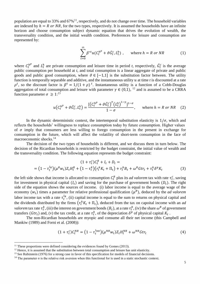
population are equal to 33% and 67%11, respectively, and do not change over time. The household variables

are indexed by ℎ = 𝑅 𝑜𝑟 𝑁𝑅, for the two types, respectively. It is assumed the households have an infinite

horizon and choose consumption subject dynamic equation that drives the evolution of wealth, the

transversality condition, and the initial wealth condition. Preferences for leisure and consumption are

represented by:

∑ 𝛽∗𝑡𝑢(𝐶𝑡ℎ𝑝

+ 𝜗�̅�𝑡𝑐, 𝐿𝑡

ℎ)

∞

𝑡=0

, where ℎ = 𝑅 𝑜𝑟 𝑁𝑅 (1)

where 𝐶𝑡ℎ𝑝

and 𝐿𝑡ℎ are private consumption and leisure time in period t, respectively, �̅�𝑡

𝑐 is the average

public consumption per household at t, and total consumption is a linear aggregate of private and public

goods and public good consumption, where 𝜗 ∈ [−1,1] is the substitution factor between. The utility

function is temporally separable and additive, and the instantaneous utility 𝑢 at time t is discounted at a rate

𝜌𝑡, so the discount factor is 𝛽𝑡 = 1/(1 + 𝜌) 𝑡. Instantaneous utility is a function of a Cobb-Douglas

aggregation of total consumption and leisure with parameter 𝛾 ∈ (0,1), 12 and is assumed to be a CRRA

function parameter 𝜎 ≥ 1:13

𝑢(𝐶𝑡ℎ𝑝

+ 𝜗�̅�𝑡𝑐, 𝐿𝑡

ℎ) =[(𝐶𝑡

ℎ𝑝+ 𝜗�̅�𝑡

𝑐)𝛾

(𝐿𝑡ℎ)

1−𝛾]1−𝜎

1 − 𝜎, where ℎ = 𝑅 𝑜𝑟 𝑁𝑅 (2)

In the dynamic deterministic context, the intertemporal substitution elasticity is 1/𝜎, which and

reflects the households’ willingness to replace consumption today by future consumption. Higher values

of 𝜎 imply that consumers are less willing to forego consumption in the present in exchange for

consumption in the future, which will affect the volatility of short-term consumption in the face of

macroeconomic shocks.14

The decision of the two types of households is different, and we discuss them in turn below. The

decision of the Ricardian households is restricted by the budget constraint, the initial value of wealth and

the transversality condition. The following equation represents the budget constraint:

(1 + 𝜏𝑡𝑐)𝐶𝑡

𝑅 + 𝐼𝑡 + 𝐷𝑡 =

= (1 − 𝜏𝑡𝑙𝑅)(𝜇𝑅𝑤𝑡)𝑍𝑡𝐻𝑡

𝑅 + (1 − 𝜏𝑡𝑘)(𝑟𝑡

𝑘𝐾𝑡 + П𝑡) + 𝑟𝑡𝑏𝐵𝑡 + 𝜔𝑅𝐺𝑡𝑟𝑡 + 𝜏𝑡

𝑘𝛿𝑝𝐾𝑡 (3)

the left side shows that income is allocated to consumption 𝐶𝑡𝑅 plus its ad valorem tax with rate 𝜏𝑡

𝑐, saving

for investment in physical capital (𝐼𝑡) and saving for the purchase of government bonds (𝐷𝑡). The right

side of the equation shows the sources of income. (i) labor income is equal to the average wage of the

economy (𝑤𝑡) times a parameter for relative professional qualification (𝜇𝑅), deduced by the ad valorem

labor income tax with a rate 𝜏𝑡𝑙𝑅 , (ii) capital income is equal to the sum to returns on physical capital and

the dividends distributed by the firms (𝑟𝑡𝑘𝐾𝑡 + П𝑡), deduced from the tax on capoital income with an ad

valorem tax rate 𝜏𝑡𝑘, (iii) the interest on government bonds (𝐵𝑡), at a rate 𝑟𝑡

𝑏, (iv) the share 𝜔𝑅 of government

transfers (𝐺𝑡𝑟𝑡) and, (v) the tax credit, at a rate 𝜏𝑡𝑘, of the depreciation 𝛿𝑝 of physical capital 𝐾𝑡 .

The non-Ricardian households are myopic and consume all their net income (this Campbell and

Mankiw (1989) and Forni et al. (2008)):

(1 + 𝜏𝑡𝑐)𝐶𝑡

𝑁𝑅 = (1 − 𝜏𝑡𝑙𝑁𝑅)(𝜇𝑁𝑅𝑤𝑡)𝑍𝑡𝐻𝑡

𝑁𝑅 + 𝜔𝑁𝑅𝐺𝑡𝑟𝑡 (4)

11 These proportions were defined considering the evidences found by Gomes (2013). 12 Hence, it is assumed that the substitution between total consumption and leisure has unit elasticity. 13 See Rubinstein (1976) for a strong case in favor of this specification for models of financial decisions. 14 The parameter σ is the relative risk aversion when this functional for is used in a static stochastic context.

6

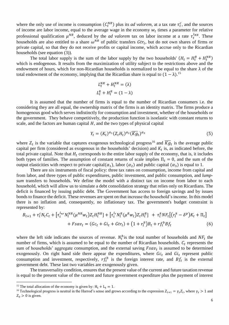
where the only use of income is consumption (𝐶𝑡𝑁𝑅) plus its ad valorem, at a tax rate 𝜏𝑡

𝑐, and the sources

of income are labor income, equal to the average wage in the economy 𝑤𝑡 times a parameter for relative

professional qualification 𝜇𝑁𝑅, deduced by the ad valorem tax on labor income at a rate 𝜏𝑡𝑙𝑁𝑅. These

households are also entitled to a share 𝜔𝑁𝑅 of public transfers 𝐺𝑡𝑟𝑡, but do not own shares of firms or

private capital, so that they do not receive profits or capital income, which accrue only to the Ricardian

households (see equation (3)).

The total labor supply is the sum of the labor supply by the two households' (𝐻𝑡 = 𝐻𝑡𝑅 + 𝐻𝑡

𝑁𝑅)

which is endogenous. It results from the maximization of utility subject to the restrictions above and the

endowment of hours, which for non-Ricardian households is normalized to be equal to the share λ of the

total endowment of the economy, implying that the Ricardian share is equal to (1 − λ).15

𝐿𝑡𝑁𝑅 + 𝐻𝑡

𝑁𝑅 = (λ)

𝐿𝑡𝑅 + 𝐻𝑡

𝑅 = (1 − λ)

It is assumed that the number of firms is equal to the number of Ricardian consumers i.e. the

considering they are all equal, the ownership matrix of the firms is an identity matrix. The firms produce a

homogenous good which serves indistinctly for consumption and investment, whether of the households or

the government. They behave competitively, the production function is isoelastic with constant returns to

scale, and the factors are human capital 𝐻, and the two types of physical capital

𝑌𝑡 = (𝐾𝑡)𝛼1(𝑍𝑡𝐻𝑡)𝛼2(𝐾𝑔̅̅ ̅̅𝑡)𝛼3 (5)

where 𝑍𝑡 is the variable that captures exogenous technological progress16 and 𝐾𝑔̅̅ ̅̅𝑡 is the average public

capital per firm (considered as exogenous in the households’ decision) and 𝐾𝑡 is, as indicated before, the

total private capital. Note that 𝐻𝑡 corresponds to the entire labor supply of the economy, that is, it includes

both types of families. The assumption of constant returns of scale implies П𝑡 = 0, and the sum of the

output elasticities with respect to private capital(𝛼1), labor (𝛼2) and public capital (𝛼3) is equal to 1.

There are six instruments of fiscal policy: three tax rates on consumption, income from capital and

from labor, and three types of public expenditures, public investment, and public consumption, and lump-

sum transfers to households. We define the model with a distinct tax on income from labor to each

household, which will allow us to simulate a debt consolidation strategy that relies only on Ricardians. The

deficit is financed by issuing public debt. The Government has access to foreign savings and by issues

bonds to finance the deficit. These revenues are spent on that increase the household’s income. In this model

there is no inflation and, consequently, no inflationary tax. The government's budget constraint is

represented by:

𝐵𝑡+1 + 𝜏𝑡𝑐𝑁𝑡𝐶𝑡 + [𝜏𝑡

𝑙𝑛𝑟𝑁𝑡𝑁𝑅(𝜇𝑁𝑅𝑤𝑡)𝑍𝑡𝐻𝑡

𝑁𝑅] + [𝜏𝑡𝑙𝑟𝑁𝑡

𝑅(𝜇𝑅𝑤𝑡)𝑍𝑡𝐻𝑡𝑅] + 𝜏𝑡

𝑘𝑁𝐹𝑡[(𝑟𝑡𝑘 − 𝛿𝑝)𝐾𝑡 + П𝑡]

+ 𝐹𝑠𝑎𝑣𝑡 = (𝐺𝑐𝑡 + 𝐺𝑖𝑡 + 𝐺𝑡𝑟𝑡) + (1 + 𝑟𝑡𝑏)𝐵𝑡 + 𝑟𝑓𝑡

𝑏𝐵𝑓𝑡 (6)

where the left side indicates the sources of revenue. 𝑁𝑡ℎis the total number of households and 𝑁𝐹𝑡 the

number of firms, which is assumed to be equal to the number of Ricardian households. 𝐶𝑡 represents the

sum of households’ aggregate consumption, and the external saving 𝐹𝑠𝑎𝑣𝑡 is assumed to be determined

exogenously. On right hand side there appear the expenditures, where 𝐺𝑐𝑡 and 𝐺𝑖𝑡 represent public

consumption and investment, respectively, 𝑟𝑓𝑡𝑏 is the foreign interest rate, and 𝐵𝑓𝑡 is the external

government debt. These last two variables are exogenously given.

The transversality condition, ensures that the present value of the current and future taxation revenue

is equal to the present value of the current and future government expenditure plus the payment of interest

15 The total allocation of the economy is given by: Ht + Lt = 1. 16 Technological progress is neutral in the Harrod’s sense and grows according to the expression 𝑍𝑡+1 = 𝛾𝑧𝑍𝑡, where 𝛾𝑧 > 1 and

𝑍0 > 0 is given.

7

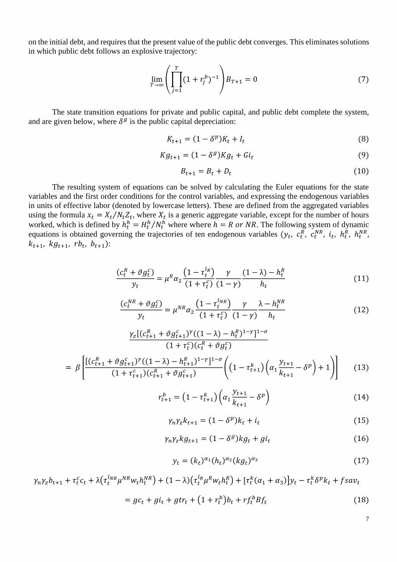
on the initial debt, and requires that the present value of the public debt converges. This eliminates solutions

in which public debt follows an explosive trajectory:

lim𝑇→∞

(∏(1 + 𝑟𝑗𝑏)−1

𝑇

𝑗=1

) 𝐵𝑇+1 = 0 (7)

The state transition equations for private and public capital, and public debt complete the system,

and are given below, where 𝛿𝑔 is the public capital depreciation:

𝐾𝑡+1 = (1 − 𝛿𝑝)𝐾𝑡 + 𝐼𝑡 (8)

𝐾𝑔𝑡+1 = (1 − 𝛿𝑔)𝐾𝑔𝑡 + 𝐺𝑖𝑡 (9)

𝐵𝑡+1 = 𝐵𝑡 + 𝐷𝑡 (10)

The resulting system of equations can be solved by calculating the Euler equations for the state

variables and the first order conditions for the control variables, and expressing the endogenous variables

in units of effective labor (denoted by lowercase letters). These are defined from the aggregated variables

using the formula 𝑥𝑡 = 𝑋𝑡 𝑁𝑡𝑍𝑡⁄ , where 𝑋𝑡 is a generic aggregate variable, except for the number of hours

worked, which is defined by ℎ𝑡ℎ = 𝐻𝑡

ℎ 𝑁𝑡ℎ⁄ where where ℎ = 𝑅 𝑜𝑟 𝑁𝑅. The following system of dynamic

equations is obtained governing the trajectories of ten endogenous variables (𝑦𝑡, 𝑐𝑡𝑅 , 𝑐𝑡

𝑁𝑅 , 𝑖𝑡, ℎ𝑡𝑅 , ℎ𝑡

𝑁𝑅 ,𝑘𝑡+1, 𝑘𝑔𝑡+1, 𝑟𝑏𝑡, 𝑏𝑡+1):

(𝑐𝑡𝑅 + 𝜗𝑔𝑡

𝑐)

𝑦𝑡= 𝜇𝑅𝛼2

(1 − 𝜏𝑡𝑙𝑅)

(1 + 𝜏𝑡𝑐)

𝛾

(1 − 𝛾)

(1 − λ) − ℎ𝑡𝑅

ℎ𝑡 (11)

(𝑐𝑡𝑁𝑅 + 𝜗𝑔𝑡

𝑐)

𝑦𝑡= 𝜇𝑁𝑅𝛼2

(1 − 𝜏𝑡𝑙𝑁𝑅)

(1 + 𝜏𝑡𝑐)

𝛾

(1 − 𝛾)

λ − ℎ𝑡𝑁𝑅

ℎ𝑡 (12)

𝛾𝑧[(𝑐𝑡+1𝑅 + 𝜗𝑔𝑡+1

𝑐 )𝛾((1 − λ) − ℎ𝑡𝑅)1−𝛾]1−𝜎

(1 + 𝜏𝑡𝑐)(𝑐𝑡

𝑅 + 𝜗𝑔𝑡𝑐)

= 𝛽 [[(𝑐𝑡+1

𝑅 + 𝜗𝑔𝑡+1𝑐 )𝛾((1 − λ) − ℎ𝑡+1

𝑅 )1−𝛾]1−𝜎

(1 + 𝜏𝑡+1𝑐 )(𝑐𝑡+1

𝑅 + 𝜗𝑔𝑡+1𝑐 )

((1 − 𝜏𝑡+1𝑘 ) (𝛼1

𝑦𝑡+1

𝑘𝑡+1− 𝛿𝑝) + 1)] (13)

𝑟𝑡+1𝑏 = (1 − 𝜏𝑡+1

𝑘 ) (𝛼1

𝑦𝑡+1

𝑘𝑡+1− 𝛿𝑝) (14)

𝛾𝑛𝛾𝑧𝑘𝑡+1 = (1 − 𝛿𝑝)𝑘𝑡 + 𝑖𝑡 (15)

𝛾𝑛𝛾𝑧𝑘𝑔𝑡+1 = (1 − 𝛿𝑔)𝑘𝑔𝑡 + 𝑔𝑖𝑡 (16)

𝑦𝑡 = (𝑘𝑡)𝛼1(ℎ𝑡)𝛼2(𝑘𝑔𝑡)𝛼3 (17)

𝛾𝑛𝛾𝑧𝑏𝑡+1 + 𝜏𝑡𝑐𝑐𝑡 + λ(𝜏𝑡

𝑙𝑁𝑅𝜇𝑁𝑅𝑤𝑡ℎ𝑡𝑁𝑅) + (1 − λ)(𝜏𝑡

𝑙𝑅𝜇𝑅𝑤𝑡ℎ𝑡𝑅) + [𝜏𝑡

𝑘(𝛼1 + 𝛼3)]𝑦𝑡 − 𝜏𝑡𝑘𝛿𝑝𝑘𝑡 + 𝑓𝑠𝑎𝑣𝑡

= 𝑔𝑐𝑡 + 𝑔𝑖𝑡 + 𝑔𝑡𝑟𝑡 + (1 + 𝑟𝑡𝑏)𝑏𝑡 + 𝑟𝑓𝑡

𝑏𝐵𝑓𝑡 (18)

8

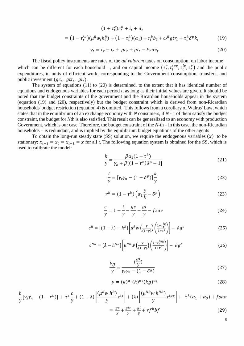
(1 + 𝜏𝑡𝑐)𝑐𝑡

𝑅 + 𝑖𝑡 + 𝑑𝑡

= (1 − 𝜏𝑡𝑙𝑅)(𝜇𝑅𝑤𝑡ℎ𝑡

𝑅) + (1 − 𝜏𝑡𝑘)(𝛼1) + 𝑟𝑡

𝑏𝑏𝑡 + 𝜔𝑅𝑔𝑡𝑟𝑡 + 𝜏𝑡𝑘𝛿𝑝𝑘𝑡 (19)

𝑦𝑡 = 𝑐𝑡 + 𝑖𝑡 + 𝑔𝑐𝑡 + 𝑔𝑖𝑡 − 𝐹𝑠𝑎𝑣𝑡 (20)

The fiscal policy instruments are rates of the ad valorem taxes on consumption, on labor income –

which can be different for each household –, and on capital income (𝜏𝑡𝑐, 𝜏𝑡

𝑙𝑁𝑅 , 𝜏𝑡𝑙𝑅 , 𝜏𝑡

𝑘) and the public

expenditures, in units of efficient work, corresponding to the Government consumption, transfers, and

public investment (𝑔𝑐𝑡, 𝑔𝑡𝑟𝑡, 𝑔𝑖𝑡).

The system of equations (11) to (20) is determined, to the extent that it has identical number of

equations and endogenous variables for each period t, as long as their initial values are given. It should be

noted that the budget constraints of the government and the Ricardian households appear in the system

(equation (19) and (20), respectively) but the budget constraint which is derived from non-Ricardian

households' budget restriction (equation 4) is omitted. This follows from a corollary of Walras' Law, which

states that in the equilibrium of an exchange economy with N consumers, if N - 1 of them satisfy the budget

constraint, the budget for Nth is also satisfied. This result can be generalized to an economy with production

Government, which is our case. Therefore, the budget constraint of the N-th – in this case, the non-Ricardian

households – is redundant, and is implied by the equilibrium budget equations of the other agents

To obtain the long-run steady state (SS) solution, we require the endogenous variables (𝑥) to be

stationary: 𝑥𝑡−1 = 𝑥𝑡 = 𝑥𝑡−1 = 𝑥 for all t. The following equation system is obtained for the SS, which is

used to calibrate the model:

𝑘

𝑦=

𝛽𝛼1(1 − 𝜏𝑘)

𝛾𝑧 + 𝛽[(1 − 𝜏𝑘)𝛿𝑝 − 1] (21)

𝑖

𝑦= [𝛾𝑧𝛾𝑛 − (1 − 𝛿𝑝)]

𝑘

𝑦 (22)

𝑟𝑏 = (1 − 𝜏𝑘) (𝛼1

𝑦

𝑘− 𝛿𝑝) (23)

𝑐

𝑦= 1 −

𝑖

𝑦−

𝑔𝑐

𝑦−

𝑔𝑖

𝑦− 𝑓𝑠𝑎𝑣 (24)

𝑐𝑅 = [(1 − 𝜆) − ℎ𝑅] [𝜇𝑅𝑤 (𝛾

(1−𝛾)) (

1−𝜏𝑡𝑙𝑅

1+𝜏𝑐 )] − 𝜗𝑔𝑐 (25)

𝑐𝑁𝑅 = [𝜆 − ℎ𝑁𝑅] [𝜇𝑁𝑅𝑤 (𝛾

(1−𝛾)) (

1−𝜏𝑡𝑙𝑁𝑅

1+𝜏𝑐 )] − 𝜗𝑔𝑐 (26)

𝑘𝑔

𝑦=

(𝑔𝑖𝑦 )

𝛾𝑧𝛾𝑛 − (1 − 𝛿𝑔) (27)

𝑦 = (𝑘)𝛼1(ℎ)𝛼2(𝑘𝑔)𝛼3 (28)

𝑏

𝑦[𝛾𝑧𝛾𝑛 − (1 − 𝑟𝑏)] + 𝜏𝑐

𝑐

𝑦+ (1 − λ) [

(𝜇𝑅𝑤 ℎ𝑅)

𝑦𝜏𝑙𝑅] + (λ) [

(𝜇𝑁𝑅𝑤 ℎ𝑁𝑅)

𝑦𝜏𝑙𝑁𝑅] + 𝜏𝑘(𝛼1 + 𝛼3) + 𝑓𝑠𝑎𝑣

= 𝑔𝑐

𝑦+

𝑔𝑡𝑟

𝑦+

𝑔𝑖

𝑦+ 𝑟𝑓𝑏𝑏𝑓 (29)

9

(1 + 𝜏𝑐)𝑐𝑅

𝑦+

𝑖

𝑦

= (1 − 𝜏𝑡𝑙𝑅)

(𝜇𝑅𝑤 ℎ𝑅)

𝑦+ (1 − 𝜏𝑘)(𝛼1) + 𝑟𝑏 𝑏

𝑦+ 𝜔𝑅 𝑔𝑡𝑟

𝑦+ 𝜏𝑡

𝑘𝛿𝑝 𝑘

𝑦 (30)

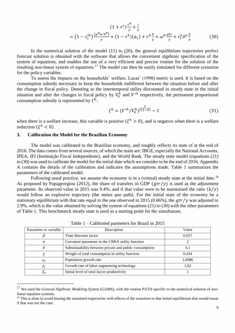
In the numerical solution of the model (11) to (20), the general equilibrium trajectories perfect

forecast solution is obtained with the software that allows the convenient algebraic specification of the

system of equations, and enables the use of a very efficient and precise routine for the solution of the

resulting non-linear system of equations.17 The model can then be easily simulated for different scenarios

for the policy variables.

To assess the impacts on the households’ welfare, Lucas’ (1990) metric is used. It is based on the

consumption subsidy necessary to keep the households indifferent between the situation before and after

the change in fiscal policy. Denoting as the intertemporal utility discounted in steady state in the initial

situation and after the changes in fiscal policy by 𝑉0ℎ and 𝑉∗ℎ respectively, the permanent proportional

consumption subsidy is represented by 𝜉ℎ:

𝜉ℎ = (𝑉∗ℎ 𝑉0ℎ⁄ )

1𝛾(1−𝜎) − 1 (31)

when there is a welfare increase, this variable is positive (𝜉ℎ > 0), and is negative when there is a welfare

reduction (𝜉ℎ < 0).

3. Calibration the Model for the Brazilian Economy

The model was calibrated to the Brazilian economy, and roughly reflects its state of at the end of

2016. The data comes from several sources, of which the main are: IBGE, especially the National Accounts,

IPEA, IFI (Instituição Fiscal Independente), and the World Bank. The steady state model (equations (21)

to (30) was used to calibrate the model for the initial date which we consider to be the end of 2016. Appendix

A contains the details of the calibration and indicates the assumptions made. Table 1 summarizes the

parameters of the calibrated model.

Following usual practice, we assume the economy is in a (virtual) steady state at the initial date.18

As proposed by Papageorgiou (2012), the share of transfers in GDP (𝑔𝑡𝑟 𝑦⁄ ) is used as the adjustment

parameter. Its observed value in 2015 was 9.4%, and if that value were to be maintained the ratio (𝑏 𝑦⁄ )

would follow an explosive trajectory (the status quo path). For the initial state of the economy be a

stationary equilibrium with that rate equal to the one observed in 2015 (0.66%), the 𝑔𝑡𝑟 𝑦⁄ was adjusted to

2.9%, which is the value obtained by solving the system of equations (21) to (30) with the other parameters

of Table 1. This benchmarck steady state is used as a starting point for the simultaions.

Table 1 – Calibrated parmeters for Brazil in 2015

Parameter or variable Description Value

𝛽 Time discount factor 0,937

𝜎 Curvature parameter in the CRRA utility function 2

𝜗 Substitutability between private and public consumption 0,1

𝛾 Weight of total consumption in utility function 0,434

𝛾𝑛 Population growth rate 1,0086

𝛾𝑧 Growth rate of labor augmenting technology 1,02

𝑍0 Initial level of total factor productivity 1

17

We used the General Algebraic Modeling System (GAMS), with the routine PATH specific to the numerical solution of non-

linear equation systems. 18 This is done to avoid biasing the simulated trajectories with effects of the transition to that initial equilibrium that would ensue

if that was not the case.

10

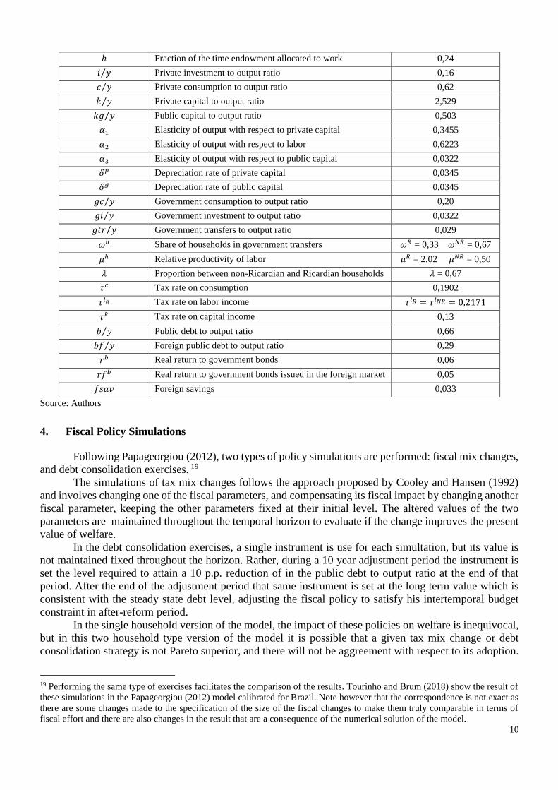
ℎ Fraction of the time endowment allocated to work 0,24

𝑖 𝑦⁄ Private investment to output ratio 0,16

𝑐 𝑦⁄ Private consumption to output ratio 0,62

𝑘 𝑦⁄ Private capital to output ratio 2,529

𝑘𝑔 𝑦⁄ Public capital to output ratio 0,503

𝛼1 Elasticity of output with respect to private capital 0,3455

𝛼2 Elasticity of output with respect to labor 0,6223

𝛼3 Elasticity of output with respect to public capital 0,0322

𝛿𝑝 Depreciation rate of private capital 0,0345

𝛿𝑔 Depreciation rate of public capital 0,0345

𝑔𝑐 𝑦⁄ Government consumption to output ratio 0,20

𝑔𝑖 𝑦⁄ Government investment to output ratio 0,0322

𝑔𝑡𝑟 𝑦⁄ Government transfers to output ratio 0,029

𝜔ℎ Share of households in government transfers 𝜔𝑅 = 0,33 𝜔𝑁𝑅 = 0,67

𝜇ℎ Relative productivity of labor 𝜇𝑅 = 2,02 𝜇𝑁𝑅 = 0,50

𝜆 Proportion between non-Ricardian and Ricardian households 𝜆 = 0,67

𝜏𝑐 Tax rate on consumption 0,1902

𝜏𝑙ℎ Tax rate on labor income 𝜏𝑙𝑅 = 𝜏𝑙𝑁𝑅 = 0,2171

𝜏𝑘 Tax rate on capital income 0,13

𝑏 𝑦⁄ Public debt to output ratio 0,66

𝑏𝑓 𝑦⁄ Foreign public debt to output ratio 0,29

𝑟𝑏 Real return to government bonds 0,06

𝑟𝑓𝑏 Real return to government bonds issued in the foreign market 0,05

𝑓𝑠𝑎𝑣 Foreign savings 0,033

Source: Authors

4. Fiscal Policy Simulations

Following Papageorgiou (2012), two types of policy simulations are performed: fiscal mix changes,

and debt consolidation exercises. 19

The simulations of tax mix changes follows the approach proposed by Cooley and Hansen (1992)

and involves changing one of the fiscal parameters, and compensating its fiscal impact by changing another

fiscal parameter, keeping the other parameters fixed at their initial level. The altered values of the two

parameters are maintained throughout the temporal horizon to evaluate if the change improves the present

value of welfare.

In the debt consolidation exercises, a single instrument is use for each simultation, but its value is

not maintained fixed throughout the horizon. Rather, during a 10 year adjustment period the instrument is

set the level required to attain a 10 p.p. reduction of in the public debt to output ratio at the end of that

period. After the end of the adjustment period that same instrument is set at the long term value which is

consistent with the steady state debt level, adjusting the fiscal policy to satisfy his intertemporal budget

constraint in after-reform period.

In the single household version of the model, the impact of these policies on welfare is inequivocal,

but in this two household type version of the model it is possible that a given tax mix change or debt

consolidation strategy is not Pareto superior, and there will not be aggreement with respect to its adoption.

19 Performing the same type of exercises facilitates the comparison of the results. Tourinho and Brum (2018) show the result of

these simulations in the Papageorgiou (2012) model calibrated for Brazil. Note however that the correspondence is not exact as

there are some changes made to the specification of the size of the fiscal changes to make them truly comparable in terms of

fiscal effort and there are also changes in the result that are a consequence of the numerical solution of the model.

11

4.1 Long-run Effects of Changes in the Tax Mix

The set of simulations for combination of different pairs of instruments produces a qualitative map

of the relative impacts of different tax mix policies. They can be organized by systematically combining the

parameters as follows. The initial change of each fiscal parameter, tax rate (𝜏𝑡𝑐, 𝜏𝑡

𝑙ℎ , 𝜏𝑡𝑘) or expenditure per

unit of efficient work (𝑔𝑐𝑡, 𝑔𝑖𝑡, 𝑔𝑡𝑟𝑡), is calibrated to represent a fiscal effort equal in the magnitude of 1%

of GDP at the initial date.20 In this simulations we admit that the change in the tax on labor income is the

same for both households21. For each, the compensating changes in the another fiscal instrument are

calculated as the solution of the system of equations (21) to (30).

The results of seventeen simulations are shown in Table 2, characterized by the values of the main

macroeconomic aggregates. They are grouped according to the policy being simulated, which is indicated

in the line "Policy", and each column of the group indicates the results of using as compensation instrument

the one shown in the line "Compensation". The line "Compensatory Variation" shows the magnitude of the

compensatory variation in percentage points, in the case of the tax rates, and as relative change with respect

to the initial value, in the case of transfers (𝑔𝑡𝑟)22. Since the trajectories to the new long-run equilibrium

are smooth, and most of them are monotonic, the effect on steady state contains all the relevant information

regarding the effects of these policies.

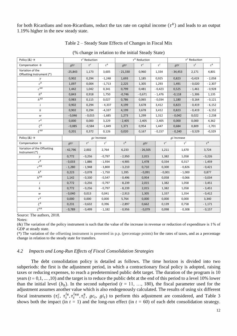
Examining the effects on the output (y), the policy that has the largest positive effect (2.02%) is the

increase in government investment (𝑔𝑖), financed by a 26.5% reduction in government transfers to

households (𝑔𝑡𝑟). However, such fiscal policy represents a welfare loss for non-Ricardian households,

since public transfers correspond to a significant portion of their budget. On the other hand, the welfare of

the Ricardian households is increased by this policy.

The policy that produces the greatest effect on aggregate consumption is a reduction in tax rate on

capital income (𝜏𝑘) with an offsetting reduction of government transfers (𝑔𝑡𝑟). It also has a significant

positive effect on output, which increases 1.69% in the long-run. The increase in consumption (𝑐) is mostly

due to a large increase in the consumption of Ricardians households (𝑐𝑅). This is also the policy that has

the greatest effect on capital stock (𝑘), and produces one of the largest marginal product of labour, which

translates into 1.27% higher wages (𝑤). The long-run impact of this policy in the number of hours worked

is positive for the non-Ricardians but negative for the Ricardians (ℎ𝑁𝑅 , ℎ𝑅).23

For the non-Ricardian households, that receive lower wages and whose budget is more dependent

on government transfers, any policy that represents a reduction in current income, be it by reducing transfers

(𝑔𝑡𝑟) or raising the tax rate on labour income (𝜏𝑙), represents a welfare loss. The exception is the policy

that reduces the tax rate on capital income with an offsetting reduction of government transfers, to which

they are indifferent. For the Ricardians households any policy that increases the tax rate on private capital

(𝜏𝑘) significantly reduces welfare, regardless of the compensating variable.

There are only two policies that increase the welfare of both households, and they use the tax rate

on consumption (𝜏𝑐) as the offsetting instrument. The one that induces the largest effect on output in the

new steady state (1.38%) is the increase in public investment (𝑔𝑖). The other policy, which is more desirable

20 Note that there is a crucial difference in relation to the tax mix proposed by Papageorgiou (2012), which follows this rule: i)

an 1% reduction in the rate of the chosen tax, compensated by the reduction of a government expenditure or an increase of

another rate; or ii) an 1% increase in any of the expenditures of the Government, in relation to their respective Steady State

levels, compensated by the increase of one of the aliquots or by the reduction of any other expenditures of the government. It is

easy to see that the 1% increase has different magnitude when applied to each of the expenditures, just as the magnitude of the

renounced revenue is different when the 1% reduction in each of the aliquots is applied. This situation can lead to misleading

results when we compare the different tax mixes. Therefore, we chose to represent the changes in the parameter always with the

reference of 1% of GDP in relation to the initial Steady State. 21 That is 𝜏𝑡

𝑙𝑅 = 𝜏𝑡𝑙𝑁𝑅 = 𝜏𝑡

𝑙. 22 It is important to note that, despite the high values of variation in the gtr, these values are small when computed as a proportion

of GDP. The values presented in Table 2 are variations in the total amount of resources allocated for transfers to households. 23 We can also highlight the contractionary effects of the policies financed by higher distortionary private capital tax rate (𝜏𝑘).

All simulated cases show that this choice leads to deleterious effects on the output in the long-run.

12

for both Ricardians and non-Ricardians, reduct the tax rate on capital income (𝜏𝑘) and leads to an output

1.19% higher in the new steady state.

Table 2 – Steady State Effects of Changes in Fiscal Mix

(% change in relation to the initial Steady State)

Policy (&) → 𝜏𝑙 Reduction 𝜏𝑘 Reduction 𝜏𝑐 Reduction

Compensation → 𝑔𝑡𝑟 𝜏𝑐 𝜏𝑘 𝑔𝑡𝑟 𝜏𝑐 𝜏𝑙 𝑔𝑡𝑟 𝜏𝑙 𝜏𝑘

Variation of the Offsetting Instrument (*)

-25,843 1,173 3,605 - 21,330 0,960 1,334 - 34,453 2,171 4,801

𝑦 0,902 0,294 -1,248 1,693 1,185 0,925 0,823 -0,419 - 2,058

𝑐𝑅 1,097 0,004 -1,713 2,225 1,305 1,293 1,491 - 0,020 - 2,307

𝑐𝑁𝑅 1,442 1,042 0,341 0,799 0,481 - 0,423 0,525 - 1,461 - 0,928

ℎ𝑅 0,843 0,918 1,750 -0,746 - 0,671 - 1,476 -0,118 - 1,306 1,135

ℎ𝑁𝑅 0,983 0,115 0,027 0,786 0,065 - 0,034 1,180 - 0,164 - 0,121

𝑖 0,902 0,294 - 4,337 4,199 3,678 3,412 0,823 - 0,419 - 6,152

𝑘 0,902 0,294 -4,337 4,199 3,678 3,412 0,823 - 0,419 - 6,152

𝑤 - 0,046 - 0,015 -1,685 1,273 1,299 1,312 - 0,042 0,022 - 2,238

𝑟𝑘 0,000 0,000 3,229 - 2,405 - 2,405 - 2,405 0,000 0,000 4,362

𝜉𝑅 - 0,085 -0,584 -1,849 1,371 0,954 1,447 0,684 0,809 -1,701

𝜉𝑁𝑅 0,201 0,372 0,126 0,020 0,167 - 0,157 - 0,240 - 0,529 -0,329

Policy (&) → 𝑔𝑐 Increase 𝑔𝑖 Increase

Compensation → 𝑔𝑡𝑟 𝜏𝑐 𝜏𝑙 𝜏𝑘 𝑔𝑡𝑟 𝜏𝑐 𝜏𝑙 𝜏𝑘

Variation of the Offsetting Instrument (*)

- 42,796 2,002 2,764 6,233 - 26,505 1,211 1,670 3,724

𝑦 0,772 - 0,256 - 0,797 - 2,950 2,015 1,382 1,058 - 0,226

𝑐𝑅 - 0,033 - 1,886 - 1,934 - 4,905 1,478 0,334 0,317 - 1,459

𝑐𝑁𝑅 - 1,280 - 1,948 - 3,800 - 3,210 0,710 0,300 - 0,826 - 0,421

ℎ𝑅 0,223 - 0,078 - 1,750 1,395 - 0,091 - 0,001 - 1,000 0,877

ℎ𝑁𝑅 1,142 - 0,330 - 0,547 - 0,496 0,954 0,058 - 0,066 - 0,034

𝑖 0,772 - 0,256 - 0,797 - 8,239 2,015 1,382 1,058 - 3,451

𝑘 0,772 - 0,256 - 0,797 - 8,239 2,015 1,382 1,058 - 3,451

𝑤 - 0,040 0,013 0,041 - 2,913 1,305 1,337 1,354 - 0,412

𝑟𝑘 0,000 0,000 0,000 5,764 0,000 0,000 0,000 3,340

𝜉𝑅 0,231 - 0,632 0,396 - 2,897 0,662 0,139 0,758 - 1,171

𝜉𝑁𝑅 - 0,789 - 0,499 - 1,182 - 0,956 - 0,079 0,098 - 0,308 - 0,157

Source: The authors, 2018.

Notes:

(&) The variation of the policy instrument is such that the value of the increase in revenue or reduction of expenditure is 1% of

GDP at steady state.

(*) The variation of the offsetting instrument is presented in p.p. (percentage points) for the rates of taxes, and as a percentage

change in relation to the steady state for transfers.

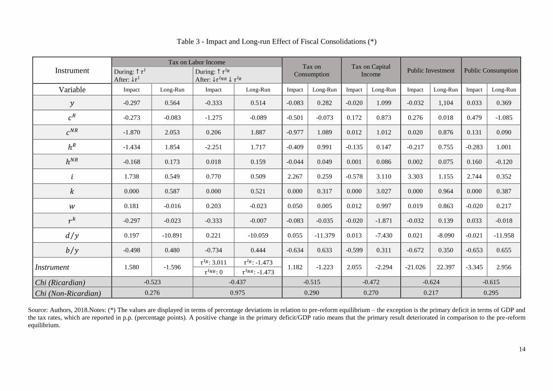
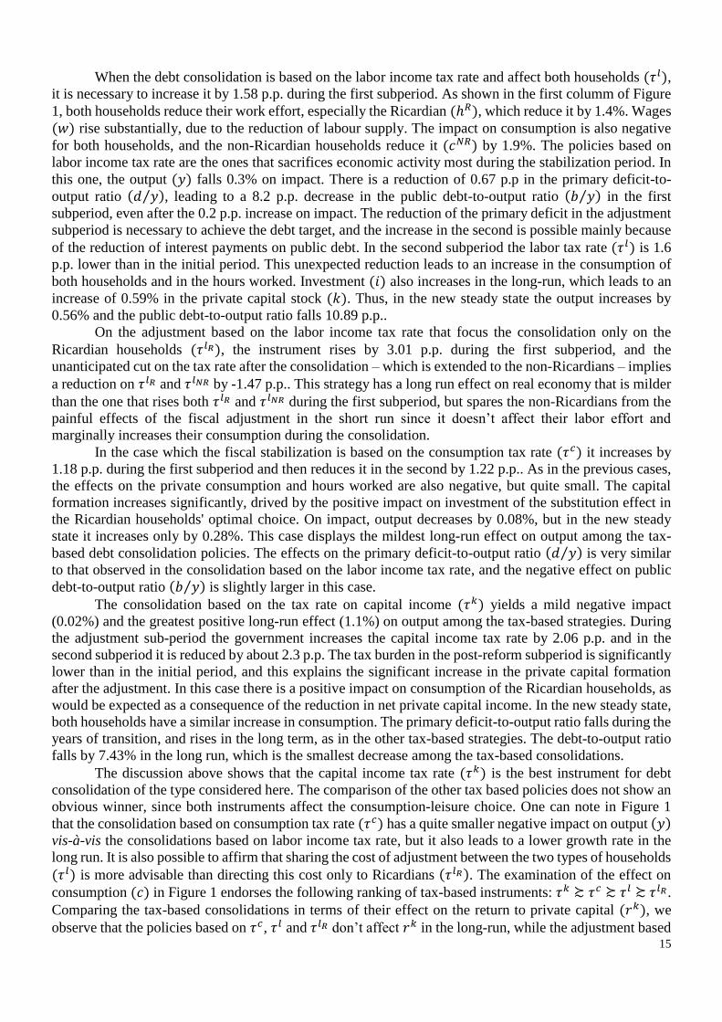
4.2 Impacts and Long-Run Effects of Fiscal Consolidation Strategies

The debt consolidation policy is detailed as follows. The time horizon is divided into two

subperiods: the first is the adjustment period, in which a contractionary fiscal policy is adopted, raising

taxes or reducing expenses, to reach a predetermined public debt target. The duration of the program is 10

years (t = 0,1, ... ,10) and the target is to reduce the public debt at the end of this period to a level 10% lower

than the initial level (𝑏0). In the second subperiod (t = 11, …, 180), the fiscal parameter used for the

adjustment assumes another value which is also endogenously calculated. The results of using six different

fiscal instruments (𝜏𝑡𝑐, 𝜏𝑡

𝑙𝑅 , 𝜏𝑡𝑙𝑁𝑅 , 𝜏𝑡

𝑘 , 𝑔𝑐𝑡, 𝑔𝑖𝑡) to perform this adjustment are considered, and Table 3

shows both the impact (in t = 1) and the long-run effect (in t = 60) of each debt consolidation strategy.

13

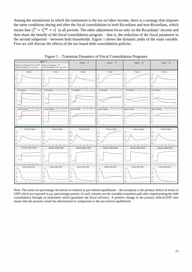
Among the simulations in which the instrument is the tax on labor income, there is a strategy that imposes

the same conditions during and after the fiscal consolidation to both Ricardians and non-Ricardians, which

means that 𝜏𝑡𝑙𝑅 = 𝜏𝑡

𝑙𝑁𝑅 = 𝜏𝑡𝑙 in all periods. The other adjustment focus only on the Ricardians’ income and

then share the benefit of the fiscal consolidation program – that is, the reduction of the fiscal parameter in

the second subperiod – between both households. Figure 1 shows the dynamic paths of the main variable.

First we will discuss the effects of the tax-based debt consolidation policies.

Figure 1 – Transition Dynamics of Fiscal Consolidation Programs

Note: The series are percentage deviations in relation to pre-reform equilibrium – the exception is the primary deficit in terms of

GDP which are reported in p.p. (percentage points). In each columm are the variables transition path after implementing the debt

consolidation through an instrument which guarantee the fiscal solvency. A positive change in the primary deficit/GDP ratio

means that the primary result has deteriorated in comparison to the pre-reform equilibrium

14

Table 3 - Impact and Long-run Effect of Fiscal Consolidations (*)

Instrument Tax on Labor Income

Tax on

Consumption Tax on Capital

Income Public Investment Public Consumption During: ↑ 𝜏𝑙

After: ↓𝜏𝑙

During: ↑ 𝜏𝑙𝑅

After: ↓𝜏𝑙𝑁𝑅 ↓ 𝜏𝑙𝑅

Variable Impact Long-Run Impact Long-Run Impact Long-Run Impact Long-Run Impact Long-Run Impact Long-Run

𝑦 -0.297 0.564 -0.333 0.514 -0.083 0.282 -0.020 1.099 -0.032 1,104 0.033 0.369

𝑐𝑅 -0.273 -0.083 -1.275 -0.089 -0.501 -0.073 0.172 0.873 0.276 0.018 0.479 -1.085

𝑐𝑁𝑅 -1.870 2.053 0.206 1.887 -0.977 1.089 0.012 1.012 0.020 0.876 0.131 0.090

ℎ𝑅 -1.434 1.854 -2.251 1.717 -0.409 0.991 -0.135 0.147 -0.217 0.755 -0.283 1.001

ℎ𝑁𝑅 -0.168 0.173 0.018 0.159 -0.044 0.049 0.001 0.086 0.002 0.075 0.160 -0.120

𝑖 1.738 0.549 0.770 0.509 2.267 0.259 -0.578 3.110 3.303 1.155 2.744 0.352

𝑘 0.000 0.587 0.000 0.521 0.000 0.317 0.000 3.027 0.000 0.964 0.000 0.387

𝑤 0.181 -0.016 0.203 -0.023 0.050 0.005 0.012 0.997 0.019 0.863 -0.020 0.217

𝑟𝑘 -0.297 -0.023 -0.333 -0.007 -0.083 -0.035 -0.020 -1.871 -0.032 0.139 0.033 -0.018

𝑑 𝑦⁄ 0.197 -10.891 0.221 -10.059 0.055 -11.379 0.013 -7.430 0.021 -8.090 -0.021 -11.958

𝑏 𝑦⁄ -0.498 0.480 -0.734 0.444 -0.634 0.633 -0.599 0.311 -0.672 0.350 -0.653 0.655

Instrument 1.580 -1.596 𝜏𝑙𝑅: 3.011 𝜏𝑙𝑅: -1.473

1.182 -1.223 2.055 -2.294 -21.026 22.397 -3.345 2.956 𝜏𝑙𝑁𝑅: 0 𝜏𝑙𝑁𝑅: -1.473

Chi (Ricardian) -0.523 -0.437 -0.515 -0.472 -0.624 -0.615

Chi (Non-Ricardian) 0.276 0.975 0.290 0.270 0.217 0.295

Source: Authors, 2018.Notes: (*) The values are displayed in terms of percentage deviations in relation to pre-reform equilibrium – the exception is the primary deficit in terms of GDP and

the tax rates, which are reported in p.p. (percentage points). A positive change in the primary deficit/GDP ratio means that the primary result deteriorated in comparison to the pre-reform

equilibrium.

15

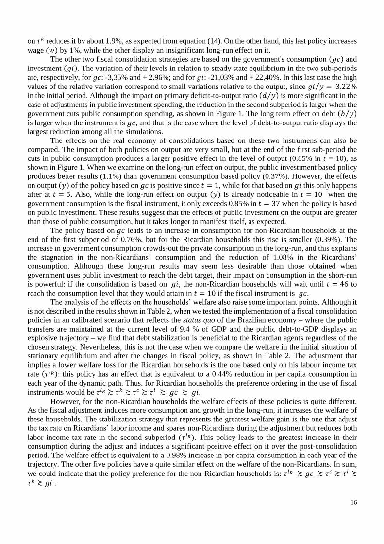
When the debt consolidation is based on the labor income tax rate and affect both households (𝜏𝑙),

it is necessary to increase it by 1.58 p.p. during the first subperiod. As shown in the first columm of Figure

1, both households reduce their work effort, especially the Ricardian (ℎ𝑅), which reduce it by 1.4%. Wages

(𝑤) rise substantially, due to the reduction of labour supply. The impact on consumption is also negative

for both households, and the non-Ricardian households reduce it (𝑐𝑁𝑅) by 1.9%. The policies based on

labor income tax rate are the ones that sacrifices economic activity most during the stabilization period. In

this one, the output (𝑦) falls 0.3% on impact. There is a reduction of 0.67 p.p in the primary deficit-to-

output ratio (𝑑 𝑦⁄ ), leading to a 8.2 p.p. decrease in the public debt-to-output ratio (𝑏 𝑦⁄ ) in the first

subperiod, even after the 0.2 p.p. increase on impact. The reduction of the primary deficit in the adjustment

subperiod is necessary to achieve the debt target, and the increase in the second is possible mainly because

of the reduction of interest payments on public debt. In the second subperiod the labor tax rate (𝜏𝑙) is 1.6

p.p. lower than in the initial period. This unexpected reduction leads to an increase in the consumption of

both households and in the hours worked. Investment (𝑖) also increases in the long-run, which leads to an

increase of 0.59% in the private capital stock (𝑘). Thus, in the new steady state the output increases by

0.56% and the public debt-to-output ratio falls 10.89 p.p..

On the adjustment based on the labor income tax rate that focus the consolidation only on the

Ricardian households (𝜏𝑙𝑅), the instrument rises by 3.01 p.p. during the first subperiod, and the

unanticipated cut on the tax rate after the consolidation – which is extended to the non-Ricardians – implies

a reduction on 𝜏𝑙𝑅 and 𝜏𝑙𝑁𝑅 by -1.47 p.p.. This strategy has a long run effect on real economy that is milder

than the one that rises both 𝜏𝑙𝑅 and 𝜏𝑙𝑁𝑅 during the first subperiod, but spares the non-Ricardians from the

painful effects of the fiscal adjustment in the short run since it doesn’t affect their labor effort and

marginally increases their consumption during the consolidation.

In the case which the fiscal stabilization is based on the consumption tax rate (𝜏𝑐) it increases by

1.18 p.p. during the first subperiod and then reduces it in the second by 1.22 p.p.. As in the previous cases,

the effects on the private consumption and hours worked are also negative, but quite small. The capital

formation increases significantly, drived by the positive impact on investment of the substitution effect in

the Ricardian households' optimal choice. On impact, output decreases by 0.08%, but in the new steady

state it increases only by 0.28%. This case displays the mildest long-run effect on output among the tax-

based debt consolidation policies. The effects on the primary deficit-to-output ratio (𝑑 𝑦⁄ ) is very similar

to that observed in the consolidation based on the labor income tax rate, and the negative effect on public

debt-to-output ratio (𝑏 𝑦⁄ ) is slightly larger in this case.

The consolidation based on the tax rate on capital income (𝜏𝑘) yields a mild negative impact

(0.02%) and the greatest positive long-run effect (1.1%) on output among the tax-based strategies. During

the adjustment sub-period the government increases the capital income tax rate by 2.06 p.p. and in the

second subperiod it is reduced by about 2.3 p.p. The tax burden in the post-reform subperiod is significantly

lower than in the initial period, and this explains the significant increase in the private capital formation

after the adjustment. In this case there is a positive impact on consumption of the Ricardian households, as

would be expected as a consequence of the reduction in net private capital income. In the new steady state,

both households have a similar increase in consumption. The primary deficit-to-output ratio falls during the

years of transition, and rises in the long term, as in the other tax-based strategies. The debt-to-output ratio

falls by 7.43% in the long run, which is the smallest decrease among the tax-based consolidations.

The discussion above shows that the capital income tax rate (𝜏𝑘) is the best instrument for debt

consolidation of the type considered here. The comparison of the other tax based policies does not show an

obvious winner, since both instruments affect the consumption-leisure choice. One can note in Figure 1

that the consolidation based on consumption tax rate (𝜏𝑐) has a quite smaller negative impact on output (𝑦)

vis-à-vis the consolidations based on labor income tax rate, but it also leads to a lower growth rate in the

long run. It is also possible to affirm that sharing the cost of adjustment between the two types of households

(𝜏𝑙) is more advisable than directing this cost only to Ricardians (𝜏𝑙𝑅). The examination of the effect on

consumption (𝑐) in Figure 1 endorses the following ranking of tax-based instruments: 𝜏𝑘 ≿ 𝜏𝑐 ≿ 𝜏𝑙 ≿ 𝜏𝑙𝑅 .

Comparing the tax-based consolidations in terms of their effect on the return to private capital (𝑟𝑘), we

observe that the policies based on 𝜏𝑐, 𝜏𝑙 and 𝜏𝑙𝑅 don’t affect 𝑟𝑘 in the long-run, while the adjustment based

16

on 𝜏𝑘 reduces it by about 1.9%, as expected from equation (14). On the other hand, this last policy increases

wage (𝑤) by 1%, while the other display an insignificant long-run effect on it.

The other two fiscal consolidation strategies are based on the government's consumption (𝑔𝑐) and

investment (𝑔𝑖). The variation of their levels in relation to steady state equilibrium in the two sub-periods

are, respectively, for 𝑔𝑐: -3,35% and + 2.96%; and for 𝑔𝑖: -21,03% and + 22,40%. In this last case the high

values of the relative variation correspond to small variations relative to the output, since 𝑔𝑖 𝑦⁄ = 3.22%

in the initial period. Although the impact on primary deficit-to-output ratio (𝑑 𝑦⁄ ) is more significant in the

case of adjustments in public investment spending, the reduction in the second subperiod is larger when the

government cuts public consumption spending, as shown in Figure 1. The long term effect on debt (𝑏 𝑦⁄ )

is larger when the instrument is 𝑔𝑐, and that is the case where the level of debt-to-output ratio displays the

largest reduction among all the simulations.

The effects on the real economy of consolidations based on these two instrumens can also be

compared. The impact of both policies on output are very small, but at the end of the first sub-period the

cuts in public consumption produces a larger positive effect in the level of output (0.85% in t = 10), as

shown in Figure 1. When we examine on the long-run effect on output, the public investiment based policy

produces better results (1.1%) than government consumption based policy (0.37%). However, the effects

on output (𝑦) of the policy based on 𝑔𝑐 is positive since 𝑡 = 1, while for that based on 𝑔𝑖 this only happens

after at 𝑡 = 5. Also, while the long-run effect on output (𝑦) is already noticeable in 𝑡 = 10 when the

government consumption is the fiscal instrument, it only exceeds 0.85% in 𝑡 = 37 when the policy is based

on public investiment. These results suggest that the effects of public investment on the output are greater

than those of public consumption, but it takes longer to manifest itself, as expected.

The policy based on 𝑔𝑐 leads to an increase in consumption for non-Ricardian households at the

end of the first subperiod of 0.76%, but for the Ricardian households this rise is smaller (0.39%). The

increase in government consumption crowds-out the private consumption in the long-run, and this explains

the stagnation in the non-Ricardians’ consumption and the reduction of 1.08% in the Ricardians’

consumption. Although these long-run results may seem less desirable than those obtained when

government uses public investment to reach the debt target, their impact on consumption in the short-run

is powerful: if the consolidation is based on 𝑔𝑖, the non-Ricardian households will wait until 𝑡 = 46 to

reach the consumption level that they would attain in 𝑡 = 10 if the fiscal instrument is 𝑔𝑐.

The analysis of the effects on the households’ welfare also raise some important points. Although it

is not described in the results shown in Table 2, when we tested the implementation of a fiscal consolidation

policies in an calibrated scenario that reflects the status quo of the Brazilian economy – where the public

transfers are maintained at the current level of 9.4 % of GDP and the public debt-to-GDP displays an

explosive trajectory – we find that debt stabilization is beneficial to the Ricardian agents regardless of the

chosen strategy. Nevertheless, this is not the case when we compare the welfare in the initial situation of

stationary equilibrium and after the changes in fiscal policy, as shown in Table 2. The adjustment that

implies a lower welfare loss for the Ricardian households is the one based only on his labour income tax

rate (𝜏𝑙𝑅): this policy has an effect that is equivalent to a 0.44% reduction in per capita consumption in

each year of the dynamic path. Thus, for Ricardian households the preference ordering in the use of fiscal

instruments would be 𝜏𝑙𝑅 ≿ 𝜏𝑘 ≿ 𝜏𝑐 ≿ 𝜏𝑙 ≿ 𝑔𝑐 ≿ 𝑔𝑖. However, for the non-Ricardian households the welfare effects of these policies is quite different.

As the fiscal adjustment induces more consumption and growth in the long-run, it increases the welfare of

these households. The stabilization strategy that represents the greatest welfare gain is the one that adjust

the tax rate on Ricardians’ labor income and spares non-Ricardians during the adjustment but reduces both

labor income tax rate in the second subperiod (𝜏𝑙𝑅). This policy leads to the greatest increase in their

consumption during the adjust and induces a significant positive effect on it over the post-consolidation

period. The welfare effect is equivalent to a 0.98% increase in per capita consumption in each year of the

trajectory. The other five policies have a quite similar effect on the welfare of the non-Ricardians. In sum,

we could indicate that the policy preference for the non-Ricardian households is: 𝜏𝑙𝑅 ≿ 𝑔𝑐 ≿ 𝜏𝑐 ≿ 𝜏𝑙 ≿

𝜏𝑘 ≿ 𝑔𝑖 .

17

5. Concluding Remarks

We examine the macroeconomic implications of fiscal reforms aimed at stimulating the economy

in the long-run and at consolidating public debt in Brazil. For this we use an extended version of the model

proposed by Papageorgiou (2012), which considers heterogeneous households: Ricardian, who have a

higher professional qualification and access to the financial market, and the non-Ricardian, who have a

relatively lower professional qualification, and therefore receive lower wages and behave like rule-of-

thumb consumers using their income exclusively for consumption since they do not have access to the

financial market. We calibrated the model for Brazil in 2015, and used it to simulate the effects of a change

in the tax mix, where a permanent reduction in one of the fiscal parameters is compensated by a permanent

increase in one of the others, and debt consolidation policies based on a single instrument.

The fiscal mix that leads to the most significant expansion of output (𝑦) in the long-run (+ 2.02%)

is the one that government increases public investment and finances it decreasing permanently the lump-

sum transfers (𝑔𝑡𝑟). The results of these exercises reveal a distributive conflict, since only two policies

lead to an increase in both households’ welfare: the reduction in tax rate on capital income (𝜏𝑘) or the

increase in public investment (𝑔𝑖), compensated by a permanent increase in tax rate on consumption (𝜏𝑐).

It is also possible to increase substantially the Ricardians’ welfare and keep the non-Ricardians indifferent,

by reducting the tax rate on capital income and compensate it through a cut in the lump-sum transfers.

The result of the debt consolidation consolidation exercises, where public debt is reduced by 10%

over the 10-year adjustment period, reveals that it is possible to increase output between 0.28% and 1.10%

in the long-run, depending on the instrument used. The consolidation based on the capital income tax rate

(𝜏𝑘) has the milder negative impact on output (- 0.02%) and the largest long-run effect (+ 1.10%) among

the tax-based strategies. The policy based on an unanticipated cut in public consumption (𝑔𝑐) has the

greatest potential to boost output during the consolidation period. None of the adjustments result in welfare

gains for the Ricardian households. The adjustment that implies a lower welfare loss for the Ricardian

households is the one based on their labor income tax rate (𝜏𝑙𝑅). This is also the scenario that offers the

most significant gain for the non-Ricardians households, to whom all simulated strategies increase welfare.

By extending the model to include heterogeneous agents we were able to capture a crucial aspect of

the Brazilian fiscal problem, which is the lack of political support for fiscal consolidation plans, evidencing

that this issue stems from the distinct effects of a given fiscal policy on different households characterized

by income inequality.

Notwithstanding the advances here, there are still remain improvements to be made to the model

that bring further insight in the design of debt consolidation programs.

Appendix - Details of the Calibration

The parameter 𝜎 that indicates the elasticity of intertemporal substitution (1 𝜎⁄ ) is of fundamental

importance for the determination of the intertemporal choices which define the trajectory of the public debt.

Lucas (1990) uses 𝜎 = 2 for the US economy, as do Baier and Glomm (2001). Lluch, Powel and Williams

(1977) estimate an extended linear expenditure (ELES) for several countries, and estimate a value for the

Frisch parameter for developing countries which implies 1 𝜎⁄ = 0.3 for Brazil. For developing countries,

Liu and Sercu (2009) estimate 1 𝜎⁄ = 0.5. Papageorgiou (2012) adopted this value for Greece, on the basis

of its widespread use. Mereb and Zilberman (2013) choose 𝜎 = 3 claiming that the empirical evidence is

scarce, and Issler and Piqueira (2000) estimate the CRRA utility function using GMM to Brazil, show that

the estimated value for 1 𝜎⁄ strongly depends periodicity of the data, and estimate (0.62) for quarterly data.

Considering this evidence, we adopted 𝜎 = 2, i.e. and 1 𝜎⁄ = 0.5.

The parameter 𝜗 that indicates the rate of substitution between public and private consumption was

set to 0.1, which is approximately the share of public spending on aggregate income.24 Baxter and King

(1993), Baier and Glomm (2001), Leeper et. al. (2010) and Papageorgiou (2012) all use that same value.

Some studies in the Brazilian literature, Ferreira and Nascimento (2006), Santana et al. (2012) and Bezerra

24 Excluding transfers from the public expenditures, we measured household consumption of public goods as the sum of

“Compensation of Employees” (4.0% of GDP) and “Other Current Expenditure” (5.3% of GDP) in the National Accounts.

18

et al. (2014) use 𝜗 = 0.5, a value which appears to be inconsistent with the revealed preference of

households.

The National Accounts (IBGE (2018)) for 2010 to 2016 were used to decompose output according

to the equation (20). The average value of the aggregates over the period was used, to reduce measurement

errors and represent more properly an approximate steady state. This does not represent any violence to the

data, because the expenditure shares were rather stable during that period except for 2016, when the share

consumption increased 2 p.p. (percentage points) to the detriment of that of public investment. To take this

into account the value for it observed in 2015 was used: 𝑐 𝑦⁄ = 0,62, and the investment share was set to

the average of 2010 to 2014: 𝑖 𝑦⁄ = 0.16.25 For the share of consumption of public goods we adopted the

value observed in 2015: 𝑔𝑐 𝑦⁄ = 0.20.

We consider that the fraction of non-Ricardian households is equal to λ = 0.67. This value is based

on the evidences found by Gomes (2013) while measuring how sensible to income is the private

consumption in Brazil. For the population growth rate we used the value in the World Bank's WDI database

for 2015, so 𝛾𝑛 = 1,0086. Following Papageorgiou (2012) we used the growth rate of per capita GDP in

the USA (2% per year) for the growth rate of labor augmenting technical progress 𝛾𝑧.26 The initial level of

the technical progress (𝑍0) set to unit. The parameter of the Cobb-Douglas consumption aggregator

function was calibrated to be consistent with so the share of hours devoted to work in the total time

endowment in the PNAD 2009 survey (IBGE (2018)): 𝛾 = 0.434 since ℎ = 0.24.

Since the production function we assumed displays constant returns of scale, the parameters can be

calculated from the factor expenditure shares. The average value of the public investment share observed

between 1995 and 2017 is, according to the IFI (2018), 𝛼3 = (𝑔𝑖 𝑦⁄ ) = 0.0322.27 For the output elasticity

of labor we follow the methodology in Gollin (2012) and calculate the share of labor income in GDP in

2015, 28 to find 𝛼2 = 0.6223, which is consistent with Ferreira and Nascimento (2006), Santana et. al.

(2012) and Mereb and Zilberman (2013). The output elasticity of private capital is calculated from the

constant returns to scale condition, 𝛼1 = 1 − 𝛼2 − 𝛼3 = 0.3455. The depreciation rate of total physical

capital was set to 3.5% per year, estimated by Gomes et al. (2003) using the permanent inventory

methodology on the investment series of the National Accounts and, use the same value for public and

private capital, 𝛿𝑝 = 𝛿𝑔 = 0.035.29

The data described previously was used to calculate the initial steady state using equation (21):

𝑘 𝑦⁄ = 2.529. Equation (27) yields 𝑘𝑔 𝑦⁄ = 0.503. 30

We used the tax rates calculated by Santana et al. (2012) for 2010, because they were deemed more

consisted with a virtual steady state for 2016 than those calculated calculuadted with 2015 data, since the

latter are distorted by the recent fiscal imbalance. The tax rates are: 𝜏𝑐 = 0,1902; 𝜏𝑙𝑟 = 𝜏𝑙𝑛𝑟 = 0,2171;

and 𝜏𝑘 = 0,13. Almeida et. al. (2017) and Azevedo and Fasolo (2015a, 2015b) show that they are

representative for the period 2010 to 2014, supporting our choice. These values are also consistent with

those calculated by Bezerra et. al. (2014), also for 2010, since the differences found can be broadly

attributed to the differences in the specification of their models.

Equation (22) was then used to calculate 𝛽 = 0.937.

25 The chosen value is very close to that established by Santana et al. (2012), which were based on the average between 1995

and 2010 and defined as 𝑖 𝑦⁄ = 0,17. 26 Barbosa Filho et. al. (2010) indicates that between 1992 and 2007 the total factor productivity in Brazil grew only 11.3%,

with an average rate of 0.71% per year. 27 Ferreira and Nascimento (2006) and Santana et. al. (2012) use endogenous growth models, and adopt a higher value for that

parameter. 28 It was calculated as (𝑅𝐸 + 𝑅𝑀𝐵) (𝑅𝐸 + 𝑅𝑀𝐵 + 𝐸𝑂𝐵)⁄ , where RE is the labor income, RMB is the Gross Mixed Income and

EOB is the Gross Operating Surplus. 29 Santana et al. (2012) also use this value. Some authors use higher depreciation rates, but they are inconsistent with the

investment series. 30 The value we find is higher than 0.3577, which is the value estimated by Bezerra et al. (2014) using data from IPEA data, but

is compatible with the data the value derived from IMF (International Monetary Fund) data for 2015, assigning half of the

private-public partnerships to public capital and the other half to private capital: 0.4494.

19

The reference for the long-run public debt/GDP ratio we adopted was the one observed in December

2015 (𝑏 𝑦⁄ = 0.66), before the recent explosive acceleration of that rate. This implicitly means that the

current level of indebtedness (0.77) is unsustainable.

We used the Fischer relation to exclude inflation from the nominal interest rate on the internal gross

debt and calculate the real rate of return on public bonds gross of taxes to be 6.88% per year. 31 The net real

interest rate on public debt is obtained by deducting from it the average tax rate on this type of income,

16.5%, obtainting a value of 5.75% per year for 2016.32 Since the analysis here is is prospective, we round

up this value, and use 𝑟𝑏 = 0.6.

The parameters that represent relative professional qualification we set 𝜇𝑛𝑟 = 0,5, based on the fact

that the minimum wage which is an indication of the productivity of the non-professionally qualified

workers which lead the non-Ricardian households is approximately half of the average wage of the private

sector in metropolitan regions, according to IBGE data. Considering the proportions of each type of

households, the Ricardians’ relative professional qualification is 𝜇𝑟 = 2,02 and which implies that the wage

of the head of Ricardian families are four times more productive.

Another dimension along which the two tipes of households differ is their share in the government

lump-sum income transfers, represented 𝜔ℎ. It was assumed that the the total transfers are distributed

evenly among the two types of households. Thus, we find that for 2015 the values 𝜔𝑛𝑟 = 0.67 and 𝜔𝑟 =0.33.

The parameters and values that represent the very simple foreign sector of our model economy are

exogenous, and were calibrated as follows. The external debt per unit of labor was assumed to remain

constant over time, and calibrated so that net external liabilities are 26% of GDP in 2016.33 The interest

rate on the external public debt was set to the sum of the average expected Fed funds rate in the US and the

average Embi+ Brazil rate, so 𝑟𝑓𝑏 = 5%. The flow of foreign savings and was also considered to be

constant over time and set to the average current account deficit between 2010 and 2015 𝑓𝑠𝑎𝑣 𝑦⁄ = 0.033.

References

ASCHAUER, D. A. Is Public Expenditure Productive ? Journal of Monetary Economics, v. 23, p. 177-200, 1989.

BAIER, S. L.; GLOMM, G. Long-run Growth and Welfare Effects of Public Policies with Distortionary

Taxation. Journal of Economic Dynamics and Control, v. 25, n. 12, p. 2007-2042, 2001.

BARBOSA FILHO, F. H. (2017) A crise econômica de 2014/2017, Estudos Avançados v. 31, n. 89, p. 51-60, 2017.

BARRO, R. J. Are Government Bonds Net Wealth?, Journal of Political Economy, v. 82, n. 6, p. 1095-1117, 1974.

BARRO, R. J., Government Spending in a Simple Model of Endogenous Growth, Journal of Political Economy v.

98, n. 5, part II, S103–S125, 1990.

BARRO, R. J.; SALA-I-MARTIN, X. Public Finance in Models of Economic Growth. Review of Economic Studies,

v.59, pp. 645-661. 1993.

BARRO, R. J.;SALA-I-MARTIN, X. Economic Growth, 2nd. edition, MIT Press, Cambridge, Massachusetts, 2004.

BAXTER, M.; KING, R. G. Fiscal Policy in General Equilibrium. The American Economic Review, v.83, p. 315-

334, 1993.

CAMPBELL, J.; MANKIW, G.N. Permanent Income, Current Income, and Consumption, Journal of Business &

Economic Statistics, v. 8, n. 3, p. 265-79. 1990.

CASELLI, F.; ESQUIVEL, G.; LEFORT, F.. Reopening the Convergence Debate: a New Look at Cross-country

Growth Empirics. Journal of Economic Growth, v. 1, n. 3, p. 363-389, 1996.

CHRISTIANO, L.J., EICHENBAUM, M., 1992. Current Real Business Cycle Theories and Aggregate Labor Market

Fluctuations, The American Economic Review v. 82, n. 3, p. 430-450. 1992.

CODACE - Comitê de Datação de Ciclos Economicos (FGV) - Comunicado de 30/10/2017. Available in

http://portalibre.fgv.br

31 The IPCA variation in 2016 was 6,29%. Source: IBGE (2018) – Synoptic Table 1 National Accounts and the gross rate of

return of domestic public debt was equal to the SELIC rate, calculated by the Central Bank of Brazil to have been 13,6% per

year on average for 2016. 32 The average is calculated considering the distribution of maturity of the total federal public debt in December 2016 (see

STN(2016)) and the maturity-dependent tax brackets (ANDIMA, 2018). 33 See Ribeiro (2016).

20

GARCIA-PEÑALOSA, C.; TURNOVSKY, S. J. Taxation and Income Distribution Dynamics in a Neoclassical

Growth Model, Journal of Money, Credit and Banking, v. 43, Issue 8, pp. 1543-1577, 2011.

GARCIA-PEÑALOSA, C.; TURNOVSKY, S. J. Income Inequality, Mobility, and the Accumulation of Capital,

Macroeconomic Dynamics v. 19, p. 1332-1357, 2015.

GIAMBIAGI, F.; ALÉM, A. C. Finanças Públicas - Teoria e Prática no Brasil - 5ª Ed., Elsevier - Editora Campus,

Brasil, 2016.

GOMES, F.A.R. Gasto do Governo e Consumo Privado: Substitutos ou Complementares?, Revista Brasileira de

Economia, v. 67 n. 2 / p. 219–234 Abr-Jun 2013.

IBGE - Instituto Brasileiro de Geografia e Estatística, Sistema de Contas Nacionais - Tabelas Sinoticas 2010- 2016,

https://www.ibge.gov.br/estatisticas-novoportal/economicas, Brasilia, 2018.

IFI - Instituição Fiscal Independente. Relatório de Acompanhamento Fiscal (RAF), Senado Federal do Brasil,

Brasília. p. 1-36. Fevereiro de 2018.

LEEPER, E.M.; YANG, S. S. Dynamic scoring: Alternative financing schemes. Journal of Public Economics, v. 92,

n. 1, p. 159-182, 2008.

LEEPER, E. M. ; WALKER, T. B.; YANG, C. S. Government investment and fiscal stimulus. Journal of Monetary

Economics v. 57, n. 8, p.1000-1012. 2010.

LUCAS, R. E. Supply-side economics: An analytical review. Oxford Economic Papers, v. 42, n. 2, p. 293-316, 1990.

MANKIW, G. N., The Savers-Spenders Theory of Fiscal Policy, American Economic Review, v. 90, n. 2, p. 120-

125. May, 2000.

PAPAGEORGIOU, D. Fiscal policy reforms in general equilibrium: The case of Greece. Journal of

Macroeconomics, v. 34, n. 2, p. 504-522, 2012.

PEREIRA, R. A.; FERREIRA, P. C. Avaliação dos impactos macroeconômicos e de bem-estar da reforma tributária

no Brasil. Revista Brasileira de Economia, v. 64, n. 2, p. 191-208, 2010.

REBELO, S. T. Long run policy analysis and long run growth. The Journal of Political Economy, v. 99, n. 3, p. 500-

521, 1991.

REINHART, Carmen M.; ROGOFF, Kenneth S. Growth in a Time of Debt, American Economic Review v. 100, n.

2, p. 573-578, 2010.

REINHART, Carmen M.; ROGOFF, Kenneth S. From Financial Crash to Debt Crisis. American Economic Review,

v. 101, p. 1676-1706, 2011.

RIBEIRO, F. J. S. P. (org.) Trajetória Futura do Saldo Transações Correntes e do Passivo Externo Líquido: Algumas

Simulações, Nota Técnica No. 20/2016, IPEA/DIMAC, Rio de Janeiro, 2016.

ROCHA, F. Long Run Limits on the Brazilian Government Debt. Revista Brasileira de Economia, v. 51, n. 4, p.

447-470, out./dez. 1997.

ROCHA, F. Política Fiscal Através do Ciclo e Operação dos Estabilizadores Fiscais, EconomiA, v.10, n.3, p. 483–

499, 2009.

ROMER, P. M., Increasing Returns and Long Run Growth, Journal of Political Economy v. 94, p. 1002–1037, 1986.

SANTANA, P.; CAVALCANTI, T. V. de V.; PAES, N. L. Impactos de Longo Prazo de Reformas Fiscais sobre a

Economia Brasileira. Revista Brasileira de Economia, v. 66, n. 2, p. 247-269, 2012.

TOURINHO, O. A. F.; BRUM, A. Políticas Fiscais para Estabilização da Dívida Pública: uma Abordagem de

Equilíbrio Geral Aplicada ao Brasil, Working paper (Submitted), 2018.

TOURINHO, O. A. F.; MERCÊS, G. M. R.; COSTA, J. G. Public Debt in Brazil: Sustentability and its Implications.

EconomiA (ANPEC), v. 14, p. 233-250, 2013.

TOURINHO, O. A. F.; SANGOI, R. Dívida Pública e Crescimento Econômico: Testes da Hipótese de Reinhart e

Rogoff, Economia Aplicada, v. 21, n. 3, p. 437-464. 2017.

TURNOVSKY, S. J.; FISHER, W. The Composition of Government Expenditure and its Consequences for

Macroeconomic Performance. Journal of Economic Dynamics and Control, v. 19, n. 4, p. 747-786. 1995.

TURNOVSKY, S. J. Optimal Tax, Debt and Expenditures Policies in a Growing Economy, Journal of Public

Economics v. 60, p. 21–44, 1996.

TURNOVSKY, S.J. Fiscal Policy in a Growing Economy with Public Capital. Macroeconomic Dynamics, v. 1, p.

615-635. 1997.

UHLIG, H. Some Fiscal Calculus. The American Economic Review, v. 100, n. 2, p. 30-34, 2010.

VINES, D.; WILLS, S. The Rebuilding Macroeconomic Theory Project: an Analytical Assessment. Oxford Review

of Economic Policy, v. 34, n.1-2, p. 1–42, 2018.

ZAGLER, M.; DÜRNECKER, G. Fiscal Policy and Economic Growth. Journal of Economic Surveys, v.17, n.3, p.

397-418. 2003.