fishr vignette stock-recruitment - derek...

$: fishR Vignette Stock-Recruitment - Derek Oglederekogle.com/fishR/examples/oldFishRVignettes/StockRecruit.pdf · \recruited to the shery." Most stock-recruit analyses will consider$
fishR Vignette - Stock-Recruitment ModelsDr. Derek Ogle, Northland College December 17, 2013

XXXX

The functions required to perform growth analyses in R are contained in the FSA and FSAdata packagesmaintained by the author and nlstools and plotrix maintained by others. These package are loaded intoR with

> library(FSA)

> library(FSAdata)

> library(nlstools)

> library(plotrix) # for plotCI()

1 Background

Quinn II and Deriso (1999) provide a simple schematic that represents the cycle of regeneration for fishpopulations (Figure 1). Most readers are likely familiar with the terms “spawners” (often time called“spawning stock” or just “stock”), “eggs”, “larvae”, and “juveniles” and have likely heard of “recruits.”However, the definition of “recruits” is very important to stock-recruit analysis and fisheries science ingeneral.

Eggs

LarvaeJuveniles

Recruits

Spawners

Figure 1. Representation of the stages in the life cycle of a fish population (adapted from Quinn II andDeriso (1999)).

In its most basic form, recruitment is the addition of young fish to the parent stock of fish. In practice,though, the definition is not as simple. Recruitment can be defined by the age of the fish. For example, fishthat have matured to an age where they are able to reproduce are said to have “recruited to the breedingpopulation” and fish that have survived to age-1 are said to have “recruited to age-1.” Some situationsrequire recruitment to be defined by the size of the fish. For example, fish that have survived to a lengthwhere they are able to reproduce are said to have “recruited to the breeding population” and fish thathave survived to a catchable size (defined by tackle, gear, or minimum size by regulation) are said to have“recruited to the fishery.” Most stock-recruit analyses will consider “recruitment to the fishery” based on sizeor “recruitment to the breeding population” based on size or age. However, as these examples illustrate, it iscritically important to explicitly define what measure of recruitment one is using in a stock-recruit analysis.

1

http://www.ncfaculty.net/dogle/

http://www.northland.edu

1.1 Density Independent Model

In the simplest models, the abundance of individuals at each stage is assumed to be proportional to theabundance of individuals at the previous stage (Quinn II and Deriso 1999). For example, if each individualin the spawning stock (S) produces an average of f eggs1 (Figure 2), then the number of eggs produced (N0)can be estimated with

N0 = fS (1)

Similarly, if g represents the probability of survival from an egg to the time of recruitment (Figure 2), thenthe number of recruits (R) can be estimated with

R = gN0 (2)

Eggs

LarvaeJuveniles

Recruits

Spawners

g

f

Eggs

LarvaeJuveniles

Recruits

Spawners

Figure 2. Representation of the stages in the life cycle of a fish population with variables representingtransition constants between some stages (adapted from Quinn II and Deriso (1999)).

If one substitutes (1) into (2) for N0 and replaces the fg product with a, then it can been seen that Ris proportional to S. As all of the models presented here are representative of an average of the responsevariable rather than the individual observations themseleves, the left-hand-side (i.e., the response side) ofthe model will be written as an expectation. Thus, in this case, R will be replaced with E[R|S] on theleft-hand-side and E[R|S] will be read as the “expected value of R given S.” Thus, the simplest non-trivialstock-recruitment model is given as

E[R|S] = aS (3)

While (3) is unrealistic, in the sense that the number of recruits can increase without bound as a functionof the number of spawners (Figure 3), it does provide some valuable insight into more realistic stock-recruitmodels to be discussed later. A simple rearrangement of (3),

R

S= a

shows that the ratio of recruits to spawners is a constant (Figure 3). In other words, the ratio of recruitsto spawners does not depend on, or is independent of, the number of spawners. For this reason, (3) is oftenreferred to as the “density independent” stock-recruitment model and a is often referred to as the “densityindependent” parameter.1Thus, f is the average net fecundity.

2

0 2000 4000 6000 8000

050

0010

000

1500

0

Spawners

Rec

ruits

0 2000 4000 6000 8000

1.5

2.0

2.5

Spawners

Rec

ruits

per

Spa

wne

r

Figure 3. Plot of number of recruits (Left) and number of recruits per spawner (Right) against numberof spawners for idealistic data constructed using equation 3, random number of spawners from a uniformdistribution between 0 and 10000, and a=2.

The density-independent model in (3) is an unrealistic model if there is any density-dependent effect onmortality, fecundity, or growth of fishes (Wootton 1990). As such, a variety of models have been developedthat extend the density-independent model by incorporating a density-dependent term. These models arediscussed in the Section 1.2 and Section 1.3.

1.2 Beverton-Holt Model

Beverton and Holt (1957) proposed a model that assumed that recruitment approached an asymptote athigh spawning stock abundance (Figure 4). Specifically, their model can be expressed as

E[R|S] =aS

1 + bS(4)

This model expresses a density-dependent relationship because the number of recruits per spawner is adecreasing function of the number of spawners (Figure 4). In (4), a is still the density-independent parameterthat is proportional to fecundity. The units of a are “recruitment per spawner” and the value of a is theslope of the model near S = 0. However, b is a density-dependent parameter that is proportional to bothfecundity and density-dependent mortality (Quinn II and Deriso 1999). If density-dependence in the stock-recruitment relationship does not exist, then b = 0 and (4) reduces to the density-independent model (3).The asymptote, or peak recruitment (denoted by Rp), of (4) is defined by Rp = a

b (Figure 4).The Beverton-Holt model is based on the assumptions that juvenile competition results in a mortality ratethat is linearly dependent upon the number of fish alive in the cohort at any time and that predators arealways present. The Beverton-Holt model is appropriate “if there is a maximum abundance imposed byfood availability or space, or if the predator can adjust its predatory activity immediately to changes in preyabundance” (Wootton 1990, p. 264).

1.2.1 Alternative Parameterizations

A model can often be cast into a different form where the model is functionally the same – i.e., predictionsare exactly the same – but it has different parameters. This alternative form is called a parameterization.All parameterizations of a model can ultimately be shown to be equivalent via algebra. Different parame-terizations of models are created for a variety of reasons, but the two most important reasons are that there-parameterized model has parameters (i) for which the interpretation meets some need and (ii) that are

3

0 2000 4000 6000 8000

020

040

060

080

0

Spawners

Rec

ruits

0 2000 4000 6000 8000

0.2

0.6

1.0

1.4

Spawners

Rec

ruits

per

Spa

wne

r

Figure 4. Plot of number of recruits (Left) and number of recruits per spawner (Right) against numberof spawners for idealistic data constructed using equation 4, random number of spawners from a uniformdistribution between 0 and 10000, a=2, and b = 0.0025. A horizontal line on the left plot is shown atab= 2

0.0025=800 for reference.

less correlated. The Beverton-Holt stock-recruitment model has been re-parameterized in a variety of ways,with the four most common re-parameterizations shown and discussed briefly below.

If Rp = ab is solved for b and substituted into (4), then the Beverton-Holt model can be re-written as

E[R|S] =aS

1 + a SRp

(5)

In this parameterization, the two parameters, a and Rp, are as defined above. Thus, this parameterizationprovides a direct estimate of the peak recruitment value.

If a = 1a and b = b

a are substituted into (4) and algebraically simplified, then the Beverton-Holt model canbe re-written as

E[R|S] =S

a+ bS(6)

In this parameterization, a is still related to density-independendence but the relationship is in the oppositedirection of a in (4) and (5). In other words, if a is “large” then a will be small. The asymptote of (6) isthen at Rp = 1

b.

Additionally, if Rp = 1b

is solved for b and substituted into (6), then the Beverton-Holt model can bere-rewritten as

E[R|S] =S

a+ SRp

(7)

As with (5), this parameterization provides a direct estimate of Rp.

All parameterizations of the Beverton-Holt model fit the data in exactly the same way (Figure 5). In addition,the correlations among model parameters do not differ substantively (Table 1). Thus, the only real reasonfor choosing any particular parameterization lies in choices you make regarding which parameters should beestimated. Throughout the remainder of this vignette the first, i.e., (4), or second, i.e., (5), parameterizationswill be used as they allow for a direct comparison to the general density independence model (i.e., (3)).

4

0 50 100 150

05

1015

Stock Level

Rec

ruitm

ent L

evel

Figure 5. Fits of the four parameterizations of the Beverton-Holt stock-recruitment model to the Lake Troutdata from area MI7 in Lake Superior. Note that the results of all fits are identical and, thus, the fitted linesare directly on top of each other. Different colors and different line widths were used to try to illustrate thispoint but may not be readily apparent on the screen or printed page.

Table 1. Parameter estimates and model results from fitting, with multiplicative errors, different parame-terizations of the Beverton-Holt stock-recruitment model (in the order presented in the text) to Lake Troutfrom area MI-7 in Lake Superior. The parameters are as defined in the text. Note that “calc Rp” is Rpcomputed from other parameters (rather than estimated directly, “SE” is the residual variability, and “r” isthe correlation coefficient between the two parameters.

Models a b a b Rp calc Rp SE r1 0.632 0.059 - - - 10.69 0.56 0.992 0.632 - - - 10.69 - 0.56 -0.823 - - 1.581 0.094 - 10.69 0.56 -0.824 - - 1.581 - 10.69 - 0.56 0.82

5

1.3 Ricker Model

Ricker (1954) proposed a stock-recruitment model that was “dome-shaped” – i.e., the peak level of recruit-ment occurred at an intermediate spawning stock abundance (Figure 6). Specifically, the Ricker model canbe expressed as

E[R|S] = aSe−bS (8)

This model expresses a density-dependent relationship because the number of recruits per spawner is adecreasing function of the number of spawners (Figure 6). In (8), a is still the density-independent parameterthat is proportional to fecundity and b is the density-dependent parameter (Quinn II and Deriso 1999). Ifdensity-dependence in the stock-recruitment relationship does not exist, then b = 0 and (8) reduces to thedensity-independent model (3). The peak level of recruitment is given by Rp = a

be and occurs at a spawningstock biomass of 1

b (Figure 6)

0 2000 4000 6000 8000

050

015

0025

00

Spawners

Rec

ruits

0 2000 4000 6000 8000

0.5

1.0

1.5

Spawners

Rec

ruits

per

Spa

wne

r

Figure 6. Plot of number of recruits (Left) and number of recruits per spawner (Right) against number ofspawners for idealistic data constructed using equation efeqn:SRRicker1, random number of spawners froma uniform distribution between 0 and 10000, a=2, and b = 0.00025. A horizontal line on the left plot isshown at a

be= 20.00025e=2943 and a vertical line is shown at 1

b= 10.00025=4000 for reference.

The Ricker stock-recruitment model assumes that the mortality rate of the eggs and juveniles is proportionalto the initial cohort size. In other words, if, for example, the inital number of eggs is high then the mortalityrate of the eggs and juveniles will also be high. Biological realities that might lead to this assumption beingmet are (1) cannibalism of the juveniles by the adults (Ricker 1975), (2) disease transmission, (3) damageby adults of one anothers spawning sites (e.g., redd superimposition), (4) density-dependent reductions ingrowth coupled with size-dependent predation (e.g., increase in the time it takes for the young fish to growthrough a size range vulnerable to predation; Ricker (1975)), and (5) a time-lag in the the response of apredator or parasite to the abundance of the fish (Wootton 1990).

1.3.1 Alternative Parameterizations

As shown with the Beverton-Holt model above, the Ricker model can also be written in different forms. Twocommon parameterizations are shown below.

Ricker (1954) commonly defined a = ea such that (8) is modified to

E[R|S] = Sea−bS (9)

With (9) the peak level of recruitment is Rp = ea

be at a stock level of 1b .

6

The first parameterization, i.e., (8), can be modified to include a parameter for the peak level of recruitmentby solving Rp = a

be for b and substituting into (8) to produce

E[R|S] = aSe−a S

Rpe (10)

Thus, fitting (10) will result in a direct estimate of the peak level of recruitment (Rp) at a stock level ofRpea .

All parameterizations of the Ricker model fit the data in exactly the same way (Figure 7). The correlationbetween model parameters was substantially lower for the third parameterization (Table 1). The first or thirdparameterizations will be used throughout the remainder of this vignette as they allow direct comparison tothe general density independence model (i.e., (3)).

0 50 100 150

05

1015

Stock Level

Rec

ruitm

ent L

evel

Figure 7. Fits of the three parameterizations of the Ricker stock-recruitment model to the Lake Trout datafrom area MI7 in Lake Superior. Note that the results of all fits are identical and, thus, the fitted lines aredirectly on top of each other. Different colors and different line widths were used to try to illustrate thispoint but may not be readily apparent on the screen or printed page.

Table 2. Parameter estimates and model results from fitting, with multiplicative errors, different param-eterizations of the Ricker stock-recruitment model to Lake Trout from area MI7 in Lake Superior. Theparameters are as defined in the text. Note that “calc Rp” is Rp computed from othe parameters (ratherthan estimated directly, “calc Sp” is the calculated stock level where the peak level of recruitment occurs,“SE” is the residual variability, and “r” is the correlation coefficient between the two parameters.

Models a b a Rp calc Rp calc Sp SE r1 0.390 0.015 - - 9.32 64.96 0.53 0.892 - 0.015 -0.941 - 9.32 64.96 0.53 0.893 0.390 - - 9.32 - 64.96 0.53 0.46

7

2 Thoughts on Model Fitting

2.1 Statistical Error Types

Most linear and non-linear model fitting algorithms assume that the random errors in the model are additiveand normal. If these errors are depicted by ε, then, for example, the Ricker2 model (8) with additive errorswould be written as (Quinn II and Deriso 1999)

R = aSe−bS + ε

Fitting the model with additive errors assumes that the variability around the model is the same in allareas of the data. It is often the case, where the variability will be greater near the peak of the model. Inthese cases, a multiplicative error structure may be more appropriate. A model with a multiplicative errorstructure is written as

R = aSe−bSeε

Most computer algorithms will not fit these models directly as the algorithm expects an additive errorstructure. However, taking natural logarithms of both sides transforms the model with a multiplicative errorstructure to one with an additive error structure (Quinn II and Deriso 1999). For example,

log(R) = log(aSe−bS) + ε

Thus, a model with a multiplicative error structure can be fit with most computer algorithms by using themodel where both sides have been logged. Because of this relationship, a multiplicative error structure isoften referred to as fitting the model with “lognormal errors.”

Fitting the model with different error structures can lead to substantially different parameter estimates(Figure 8). While one should carefully examine the residuals of each fitted model, Quinn II and Deriso(1999) suggest that the theory used to develop the Beverton-Holt and Ricker models suggests that themultiplicative error model should be the default choice. They also suggest that the multiplicative errormodel “fits the error structure of actual data sets fairly well” (Quinn II and Deriso 1999, p. 104).

0 500 1500 2500

010

000

2000

030

000

spawner

recr

uit

MultiplicativeAdditive

Figure 8. Number of recruits versus number of spawners for Escanaba Lake Walleye with the Ricker stock-recruitment model fit with additive and multiplicative errors superimposed.

2.2 Variability

Stock-recruitment data is notoriously “messy” with large year-to-year variability in recruitment (Figure 9)and a weak relationship between spawning stock and number of recruits (Figure 10). This variability or the

2From hereon the term “Ricker” model and “Beverton-Holt” model will refer to the first parameterizations of each model.

8

resultant difficulties in fitting or interpreting stock-recruitment models has been commented on by severalauthors:

Much ingenuity has been spent in fitting these curves to data sets and to developing the basicmodels. All this effort has largely foundered in the face of the variability in the relationshipsbetween stock and recruitment shown by most natural populations. The curves can be fitted,but it takes an act of faith to take the resulting curves seriously. – (Wootton 1990, p. 264)

Empirical relationships between spawning stock and recruitment shown extreme annual variabil-ity. – (Quinn II and Deriso 1999, p. 86)

... a number of tools are available for the analysis of stock and recruitment, but there are manypitfalls awaiting the unwary biologist who want to fit a curve and get an answer. ...

Analysis of stock-recruitment data provides an enormous number of traps for the unwary – goodluck. (Hilborn and Walters 2001, p. 295)

1982 1986 1990 1994

050

015

0025

00

Vendace −− Finland

Year

Age

−0+

Fis

h pe

r ha

1980 1985 1990 1995 2000

12

34

White Shrimp −− Georgia

Year

Com

mer

cial

Lan

ding

s (A

ug−

Jan)

1975 1980 1985 1990

24

68

1012

14

Lake Trout −− Lake Superior

Year

CP

UE

Age

−7

Fis

h

1980 1985 1990 1995

020

040

060

080

0

Rainbow Smelt −− Lake Erie

Year

Num

ber

per

Hou

r

1982 1986 1990 1994

050

015

0025

00

Yellow Perch −− Lake Huron

Year

Num

ber

per

Set

1960 1964 1968 1972

02

46

810

12

Walleye −− Lake Erie

Num

ber

per

1000

ft

Figure 9. Plot of number of recruits versus year for a variety of species.

9

0 2 4 6 8 10 12 14

050

015

0025

00Vendace −− Finland

Age−1+ Fish Biomass (kg/ha)

Age

−0+

Fis

h pe

r ha

0 5 10 15

12

34

White Shrimp −− Georgia

CPUE in JuneC

omm

erci

al L

andi

ngs

(Aug

−Ja

n)

50 100 150 200

24

68

1012

14

Lake Trout −− Lake Superior

CPUE of Age−8+ Fish

CP

UE

Age

−7

Fis

h

0 2 4 6 8 10 12 14

050

015

0025

00Yellow Perch −− Lake Huron

Spawning Stock (Number per Set)

Rec

ruits

(N

umbe

r pe

r S

et)

40000 60000 80000

3000

5000

7000

Pacific Flounder

Spawning Stock Biomass (Tonnes)

Num

ber

of R

ecru

its (

Tho

usan

ds)

0e+00 2e+05 4e+05 6e+05

050

0000

1000

000

1500

000 Herring −− Iceland

Spawning Stock Biomass (Tonnes)

Num

ber

of A

ge−

1 (T

hous

ands

)

Figure 10. Plot of number of recruits versus spawning stock for a variety of species.

10

2.3 Starting Values

The Beverton-Holt and Ricker stock-recruit models are best fit using non-linear regression methods. Non-linear regression methods use an iterative algorithm that requires starting values for the model parameters.There are at least two ways to arrive at reasonable starting values for the parameters of the Beverton-Holt and Ricker stock-recruit models – (i) estimation from linearized models and (ii) visual estimation withdynamics graphics. Both methods are discussed below.

The first parameterization of the Beverton-Holt model can be viewed as a linear function as shown in (11)3.Thus, a linear regression of the inverse of R (i.e., 1

R ) on the inverse of S (i.e., 1S ) will yield an equation where

the slope is equal to 1a and the intercept is equal to b

a . The slope and intercept equivalents can be solvedfor a and b to derive reasonable starting values for the non-linear regression algorithm. Starting values forother parameters in the other parameterizations can be derived by using the starting values of a and b inthe parameter equivalency equations.

1

E[R|S]=

1

a

1

S+b

a(11)

The first parameterizaton of the Ricker model can be viewed as a linear function as shown in (12)4. Thus, alinear regression of the log of R

S on S will yield an equation where the slope is equal to −b and the interceptis equal to log(a). Again, the slope and intercept equivalents can be solved for a and b to derive reasonablestarting values. Starting values for the other parameters in the other parameterizations can be derived byusing the starting values for a and b in the parameter equivalency equations.

log

(E[R|S]

S

)= log(a)− bS (12)

The methodology described above has been implemented in srStarts() and is described in more detail inSection 3.

The selection of starting values for the stock-recruit models can also be easily estimated with srSim() fromthe FSATeach package5. This function produces a plot of R versus S with a stock-recruit model superimposed.The parameters of the superimposed stock-recruit model can be controlled with slider bars. Thus, the sliderbars can be adjusted until a model is produced that “roughly” fits the observed recruit versus stock graphic.The parameters of the model when this rough fit is found can then be used as the starting values for thenon-linear methods. For this purpose, srSim() has the same four arguments as srStart(). As an example,the starting values for the first parameterization of the Beverton-Holt model is shown by the slider bars onthe graphic (Figure 11) produced with

> srSim(recruits~stock,data=LakeTroutGIS,type="BevertonHolt",param=1)

2.4 Assumption Checking

The non-linear regression, as it has been described here, requires that the variability about the model isconstant (i.e., homoscedasticity), the errors are normally distributed, the model adequately fits the data,and there are no influential or outlying points. There are tests to determine if these assumptions have beenviolated, but these tests can be hyper-sensitive (i.e., tend to identify assumption violations) especially withlarge sample sizes. Thus, the adequacy of meeting these assumptions can be better determined by objectivelyanalyzing two important graphics. The first graphic is a residual plot which plots the model residuals versusthe fitted values (Figure 12-Left). In general, the assumptions of the model are met if NO pattern is observed

3Note that the critical step in deriving this model is to first invert both sides of (4).4Again, the critical first step in deriving this function is inverting the original function (8).5Note that the FSATeach package must be installed as described here and the loaded with library(FSATeach).

11

http://www.rforge.net/FSATeach/Installation.html

Figure 11. Example of using srSim() to find an approximate fit of the first parameterization of the Beverton-Holt stock-recruitment model to the Gull Island Shoal Lake Trout data.

in the residual plot. Curvature in this plot would suggest that the model does not represent the data verywell and a “funneling” from left-to-right would suggest that the variability around the model is not constant(i.e., heteroscedasticity). The second graphic is a histogram of the residuals (Figure 12-Right). In general,the assumption of normality is adequately met if this histogram is symmetric without overly long “tails.”

1.6 1.8 2.0 2.2

−1.

0−

0.5

0.0

0.5

1.0

Fitted Values

Res

idua

ls

residuals(Abh1r)

Fre

quen

cy

−1.5 −0.5 0.5 1.0 1.5

01

23

45

67

Figure 12. Residual plot (left) and residual histogram (right) from fitting the first parameterization of thestock-recruit model to the Lake Superior Lake Trout from area MI7 data.

The residual plot can be constructed by submitting the saved nls object to residPlot(). The histogramcan be constructed by submitting the saved nls object to residuals() and then submitting this result tohist(). Interpretation of these graphics will be discussed further in the context of the examples in thefollowing section.

3 Fitting Basic Models in R

Both the Beverton-Holt and Ricker stock-recruit models can be linearized and fit with least-square simplelinear regression. However, the models can also be fit with non-linear least-squares methods that providesimilar parameter estimates but provides a method that is more general and extensible. Fitting non-linearmodels in R is described in detail in the Von Bertalanffy Growth Model vignette. Briefly, the non-linearmodel fitting procedure in R is implemented with nls(), which requires the model formula, the list ofstarting values, and the data frame as arguments. In addition, trace=TRUE can be included in nls() to seethe residual sum-of-squares and current values of the parameters for each iteration of the fitting process. For

12

simplicity and clarity, the starting values can be entered into a list and the formula can be created prior tocalling nls(). The use of nls() is illustrated with the following examples.

The mean catch-per-unit-effort of adult female Lake Trout per 1000 m of gillnet from fall spawning surveys(i.e., the “stock”) and the density of age-0 fish per ha captured the following fall in bottom trawls (i.e., the“recruits”) were recorded from an area near Gull Island Shoal in the Apostle Islands region of Lake Superior(Schram et al. 1995). These data are loaded and the structure is observed with

> data(LakeTroutGIS)

> str(LakeTroutGIS)

'data.frame': 28 obs. of 3 variables:

$ year : int 1964 1965 1966 1967 1968 1969 1970 1971 1972 1973 ...

$ stock : num 9.06 15 13.33 15.04 15.56 ...

$ recruits: num 11.12 2.06 9.87 9.05 2.06 ...

In order to fit a stock-recruitment model with multiplicative errors, a new variable consisting of the naturallog of the “recruit” variable must be constructed and appended to the data frame with

> LakeTroutGIS$logR <- log(LakeTroutGIS$recruit)

> str(LakeTroutGIS)


$ year : int 1964 1965 1966 1967 1968 1969 1970 1971 1972 1973 ...

$ stock : num 9.06 15 13.33 15.04 15.56 ...

$ recruits: num 11.12 2.06 9.87 9.05 2.06 ...

$ logR : num 2.409 0.721 2.289 2.203 0.723 ...

3.1 Fitting Beverton-Holt Model in R – Case I

The linear models used to generate starting values discussed previously are implemented in R with srStarts().This function which requires a model of the generic form R~S as the first argument, the data frame fromwhich to find R and S in the data= argument, the type of model (either "BevertonHolt" or "Ricker") inthe type= argument, and the “number” of the parameterization in the param= argument. The “numbers”’used in param= correspond to the order the parameterizations were presented in this vignette6. Startingvalues for the Lake Trout example were generated, and saved to an object, with

> bh1s <- srStarts(recruits~stock,data=LakeTroutGIS,type="BevertonHolt",param=1)

> unlist(bh1s) # unlist used just to save space when displaying

a b

0.36437 0.01857

For simplicity, the Beverton-Holt model should be declared and saved to an object before proceeding to usenls(). For example, the first parameterization is declared with7

> bh1 <- logR~log((a*stock)/(1+b*stock))

The Beverton-Holt model is then fit and saved to an object with8

6The models can also be seen with srModels()7The srFuns() function can be used to declare this and other stock-recruit model functions. In this case, one would use bh1

<- srFuns(type="BevertonHolt",param=1).8If the model bh1 was declared using srFuns(), then one would need to use bh1nls <-

nls(logR~log(bh1(stock,a,b)),data=LakeTroutGIS,start=bh1s) to fit the model here.

13

> bh1nls <- nls(bh1,data=LakeTroutGIS,start=bh1s)

For comparative purposes the density-independence model is fit and saved to an object with

> bh0 <- logR~log(a*stock) # declare model

> bh0s <- bh1s[1] # use the same starting value as above for a

> bh0nls <- nls(bh0,data=LakeTroutGIS,start=bh0s)

An “extra sums-of-squares” test and AIC calculations for determining whether the density independence orBeverton-Holt model “best” fits the data is computed with

> anova(bh0nls,bh1nls)

Analysis of Variance Table

Model 1: logR ~ log(a * stock)

Model 2: logR ~ log((a * stock)/(1 + b * stock))

Res.Df Res.Sum Sq Df Sum Sq F value Pr(>F)

1 27 14.6

2 26 13.7 1 0.821 1.55 0.22

> AIC(bh0nls,bh1nls)

df AIC

bh0nls 2 65.16

bh1nls 3 65.53

With a large p-value (p = 0.22) for the ANOVA and a larger AIC value, it is clear that the Beverton-Holt model does NOT explain significantly more of the variability in recruitment then a simple density-independence model. Thus, the Beverton-Holt model with the density-dependent parameter does NOTappear to be a “better” fit for these data.

A graphic (Figure ??) depicting the relative fit of these two models can be constructed, from the “groundup”, as shown with

> plot(recruits~stock,data=LakeTroutGIS)

> curve((coef(bh1nls)[1]*x)/(1+coef(bh1nls)[2]*x),from=0,to=120,col="red",lwd=2,add=TRUE)

> curve(coef(bh0nls)[1]*x,from=0,to=120,col="blue",lwd=2,add=TRUE)

> legend("topleft",legend=c("density independent","density dependent"),

col=c("blue","red"),lwd=2,cex=0.6)

The parameter estimates, along with other summary results, are obtained by submitting the saved nls()

object to overview() from the nlstools package. Because the Beverton-Holt model was not a “better” fit,this is demonstrated below for the Beverton-Hold model for illustrative purposes only,

> overview(bh1nls)

------

Formula: logR ~ log((a * stock)/(1 + b * stock))

Parameters:

Estimate Std. Error t value Pr(>|t|)

a 0.38276 0.11470 3.34 0.0026

b 0.00736 0.00809 0.91 0.3711

Residual standard error: 0.727 on 26 degrees of freedom

14

20 40 60 80 100

010

2030

40stock

recr

uits

density independentdensity dependent

Figure 13. Plot of recruitment versus stock levels for the Gull Island Shoal Lake Trout data with theBeverton-Holt and simple density-independence stock-recruit models superimposed.

Number of iterations to convergence: 4

Achieved convergence tolerance: 2.9e-07

------

Residual sum of squares: 13.7

------

Asymptotic confidence interval:

2.5% 97.5%

a 0.146988 0.61853

b -0.009262 0.02398

------

Correlation matrix:

a b

a 1.0000 0.8887

b 0.8887 1.0000

The asymptotic confidence intervals and hypothesis tests in the results above should generally not be trusted.Instead 200 bootstrap samples are constructed with

> bootbh1 <- nlsBoot(bh1nls,niter=200) # B=200 is too low, should be nearer B=1000

Warning: NaNs produced



Warning: The fit did not converge 3 times during bootstrapping

and 95% bootstrap confidence intervals are obtained and visualized (Figure 14) with

> confint(bootbh1,plot=TRUE)

95% LCI 95% UCI

a 0.247739 0.80408

b -0.001815 0.04037

15

a

Fre

quen

cy

0.2 0.4 0.6 0.8 1.0

010

2030

4050

60

b

Fre

quen

cy

0.00 0.02 0.04

010

2030

4050

Figure 14. Histogram of the bootstrap results for the Beverton-Holt stock-recruit model fit to the Gull IslandShoal Lake Trout data. Red horizontal lines represent the 95% bootstrap confidence intervals.

The skewed distribution of the bootstrap results for both parameters suggests that the asympotic CIs andtests in the overview() output are likely biased. In addition, note that the bootstrap CI for b suggests thatb could be equal to zero, further suggesting that the density dependent paramater is not warranted for thesedata.

Finally, a scatterplot of the bootstrap estimates of the parameters, constructed below and seen in (Figure15), shows a strong correlation between the two parameters.

> plot(bootbh1)

+

++

+ +

+

++

+

+

+

+

+

+

+

++

+

+

+

+

+

+ + ++

+

+

+

+

++

+

++

+

++

++

++

+

+

+

++

+

+

+

+

+

+

++

+++

+

+

++++

++

+

+

++

++

+

+

+

+

++

+

+

+

+

+

+

+

+

+

+

++

+

+

+

+

+

++

+

+

+

+

++

++

+ ++

+

+

+

+

++++

+++

++

+

++

++

++

++

++

++

+

+

+

+

+

++

+

+

++

+

++

+

+

+

+

+

+

+

+

++

++

+

+

+

+

+

+ +

++

++

+

+

+

+

+

+

+

++++

++

+

+

+

+

++

++

+

+

+

++

0.2 0.4 0.6 0.8

0.00

0.02

0.04

a

b

Figure 15. Scatterplot for the parameters of the bootstrap results for the Beverton-Holt stock-recruit modelfit the Gull Island Shoal Lake Trout data.

16

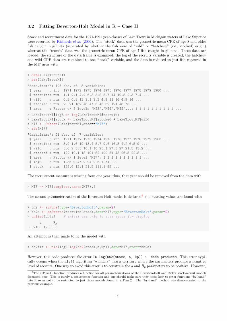
3.2 Fitting Beverton-Holt Model in R – Case II

Stock and recruitment data for the 1971-1991 year-classes of Lake Trout in Michigan waters of Lake Superiorwere recorded by Richards et al. (2004). The “stock” data was the geometric mean CPE of age-8 and olderfish caught in gillnets (separated by whether the fish were of “wild” or “hatchery” (i.e., stocked) origin)whereas the “recruit” data was the geometric mean CPE of age-7 fish caught in gillnets. These data areloaded, the structure of the data frame is examined, the log of the recruits variable is created, the hatcheryand wild CPE data are combined to one “stock” variable, and the data is reduced to just fish captured inthe MI7 area with

> data(LakeTroutMI)

> str(LakeTroutMI)


$ year : int 1971 1972 1973 1974 1975 1976 1977 1978 1979 1980 ...

$ recruits: num 1.1 2.1 4.2 6.3 3.8 5.7 14 10.8 2.3 7.4 ...

$ wild : num 0.2 0.5 12 3.1 3.2 4.8 11 16 4.9 14 ...

$ stocked : num 20 21 182 48 47.5 46 69 121 48 75 ...

$ area : Factor w/ 5 levels "MI3","MI4","MI5",..: 1 1 1 1 1 1 1 1 1 1 ...

> LakeTroutMI$logR <- log(LakeTroutMI$recruit)

> LakeTroutMI$stock <- LakeTroutMI$stocked + LakeTroutMI$wild

> MI7 <- Subset(LakeTroutMI,area=="MI7")

> str(MI7)


$ year : int 1971 1972 1973 1974 1975 1976 1977 1978 1979 1980 ...

$ recruits: num 3.9 1.6 19 13.4 5.7 9.6 16.8 4.2 6.5 9 ...

$ wild : num 3.6 2 3.5 10.1 10 25.1 27.3 27 21.5 13.2 ...

$ stocked : num 122 10.1 18 101 82 100 51 48 26.5 22.8 ...

$ area : Factor w/ 1 level "MI7": 1 1 1 1 1 1 1 1 1 1 ...

$ logR : num 1.36 0.47 2.94 2.6 1.74 ...

$ stock : num 125.6 12.1 21.5 111.1 92 ...

The recruitment measure is missing from one year; thus, that year should be removed from the data with

> MI7 <- MI7[complete.cases(MI7),]

The second parameterization of the Beverton-Holt model is declared9 and starting values are found with

> bh2 <- srFuns(type="BevertonHolt",param=2)

> bh2s <- srStarts(recruits~stock,data=MI7,type="BevertonHolt",param=2)

> unlist(bh2s) # unlist use only to save space for display

a Rp

0.2153 19.0000

An attempt is then made to fit the model with

> bh2fit <- nls(logR~log(bh2(stock,a,Rp)),data=MI7,start=bh2s)

However, this code produces the error In log(bh2(stock, a, Rp)) : NaNs produced. This error typi-cally occurs when the nls() algorithm “wanders” into a territory where the parameters produce a negativelevel of recruits. One way to avoid this error is to constrain the a and Rp parameters to be positive. However,

9The srFuns() function produces a function for all parameterizations of the Beverton-Holt and Ricker stock-recruit modelsdiscussed here. This is purely a convenience function and one should make sure they know how to enter functions “by-hand”into R so as not to be restricted to just those models found in srFuns(). The “by-hand” method was demonstrated in theprevious example.

17

the default optimization algorithm in nls() does not support constrained parameters. Therefore, the opti-mization algorithm needs to be changed to the so-called “port” algorithm which does support constrainedparameter choices. The optimization algorithm is changed with algorithm="port" and lower bounds ofzero are set for both parameters with lower=c(0,0). Thus, the constrained model is fit and saved to anobject with

> bh2fit <- nls(logR~log(bh2(stock,a,Rp)),data=MI7,start=bh2s,algorithm="port",lower=c(0,0))

The density-independence model is fit to these data with

> bh0 <- logR~log(a*stock)

> bh0s <- bh2s[1]

> bh0fit <- nls(bh0,data=MI7,start=bh0s,algorithm="port",lower=c(0))

The “extra sum-of-squares” test and AIC results to compare these two models are computed with

> anova(bh0fit,bh2fit)



Model 2: logR ~ log(bh2(stock, a, Rp))


1 19 10.55

2 18 5.67 1 4.88 15.5 0.00097

> AIC(bh0fit,bh2fit)

df AIC

bh0fit 2 47.96

bh2fit 3 37.54

Both a “small” p-value (p = 0.0010) and the smaller AIC value suggest that the Beverton-Holt model withthe density-dependent parameter provide a “better” fit to the data then the simple density-independencemodel. A supporting graphic (Figure ??) is constructed with

> plot(recruits~stock,data=MI7,pch=19)

> curve(bh2(x,coef(bh2fit)[1],coef(bh2fit)[2]),from=0,to=130,col="red",lwd=2,add=TRUE)

> curve(coef(bh0fit)[1]*x,from=0,to=130,col="blue",lwd=2,add=TRUE)

> legend("topright",legend=c("density independent","density dependent"),col=c("blue","red"),

lwd=2,cex=0.6)

The parameter estimates, along with other summary results, are obtained with

> overview(bh2fit)

------

Formula: logR ~ log(bh2(stock, a, Rp))

Parameters:


a 0.632 0.499 1.27 0.2213

Rp 10.691 3.107 3.44 0.0029


18

20 40 60 80 100 120

510

15stock

recr

uits


Figure 16. Plot of recruitment versus stock levels for the Lake Superior MI7 area Lake Trout data with theBeverton-Holt and simple density-independence stock-recruit models superimposed.

Algorithm "port", convergence message: relative convergence (4)

------


------


2.5% 97.5%

a -0.4163 1.681

Rp 4.1634 17.218

------

Correlation matrix:

a Rp

a 1.0000 -0.8219

Rp -0.8219 1.0000

The 95% bootstrap confidence intervals are obtained and visualized (Figure 17) with

> bootbh2 <- nlsBoot(bh2fit,niter=200) # B=200 is too low, should be nearer B=1000

Warning: The fit did not converge 41 times during bootstrapping

> confint(bootbh2,plot=TRUE)

95% LCI 95% UCI

a 0.309 8.005

Rp 7.218 17.088

The bootstrap results show a strongly skewed distribution for a. The Rp distribution is less skewed andapproximate 95% confidence intervals for Rp is between 7.2 and 17.1.

19

a

Fre

quen

cy

0 5 10 15 20

020

4060

8012

0

Rp

Fre

quen

cy

6 8 10 12 14 16 18 20

010

2030

4050

Figure 17. Histogram of the bootstrap results for the Beverton-Holt stock-recruit model fit to the LakeSuperior MI7 area Lake Trout data. Red horizontal lines represent the 95% bootstrap confidence intervals.

20

3.3 Fitting the Ricker Model in R

The fitting of the third parameterization of the Ricker model is illustrated with Lake Trout data from LakeSuperior’s MI7 area. The third parameterization of the Ricker model is declared and starting values arefound with

> r3 <- srFuns(type="Ricker",param=3)

> r3s <- srStarts(recruits~stock,data=MI7,type="Ricker",param=3)

> unlist(r3s) # unlist use only to save space for display

a Rp

0.3901 9.3217

The model is then fit and saved to an object with

> r3fit <- nls(logR~log(r3(stock,a,Rp)),data=MI7,start=r3s,algorithm="port",lower=c(0,0))

The density-independence model is fit and the “extra sum-of-squares” test and AIC results computed with

> r0 <- logR~log(a*stock)

> r0s <- r3s[1]

> r0fit <- nls(r0,data=MI7,start=r0s,algorithm="port",lower=c(0))

> anova(r0fit,r3fit)



Model 2: logR ~ log(r3(stock, a, Rp))


1 19 10.55

2 18 5.15 1 5.39 18.9 0.00039

> AIC(r0fit,r3fit)

df AIC

r0fit 2 47.96

r3fit 3 35.63

Both a “small” p-value (p = 0.0004) and the smaller AIC value suggest that the Ricker model with thedensity-dependent parameter provide a “better” fit to the data then the simple density-independence model.A supporting graphic (Figure ??) is constructed with

> plot(recruits~stock,data=MI7,pch=19)

> curve(r3(x,coef(r3fit)[1],coef(r3fit)[2]),from=0,to=130,col="red",lwd=2,add=TRUE)

> curve(coef(r0fit)[1]*x,from=0,to=130,col="blue",lwd=2,add=TRUE)

> legend("topright",legend=c("density independent","density dependent"),col=c("blue","red"),

lwd=2,cex=0.6)

The parameter estimates, along with other summary results, are obtained with

> overview(r3fit)

------

Formula: logR ~ log(r3(stock, a, Rp))

21

20 40 60 80 100 120

510

15stock

recr

uits


Figure 18. Plot of recruitment versus stock levels for the Lake Superior MI7 area Lake Trout data with theRicker and simple density-independence stock-recruit models superimposed.

Parameters:


a 0.390 0.101 3.85 0.0012

Rp 9.322 1.115 8.36 1.3e-07


Algorithm "port", convergence message: both X-convergence and relative convergence (5)

------


------


2.5% 97.5%

a 0.1773 0.6029

Rp 6.9790 11.6644

------

Correlation matrix:

a Rp

a 1.0000 0.4613

Rp 0.4613 1.0000

The 95% bootstrap confidence intervals are obtained and visualized (Figure 19) with

> bootr3 <- nlsBoot(r3fit,niter=200) # B=200 is too low, it should be nearer B=1000

> confint(bootr3,plot=TRUE)

95% LCI 95% UCI

a 0.2478 0.6228

Rp 7.6325 11.8094

The bootstrap results show a moderately skewed distribution for both a andRp. Approximate 95% confidenceintervals for Rp is between 7.6 and 11.8.

One can compute a confidence interval for the stock level that corresponds to the peak recruitment level by

22

a

Fre

quen

cy

0.2 0.3 0.4 0.5 0.6 0.7

010

2030

Rp

Fre

quen

cy

7 8 9 10 11 12 13

010

2030

40

Figure 19. Histogram of the bootstrap results for the Ricker stock-recruit model fit to the Lake SuperiorMI7 area Lake Trout data. Red horizontal lines represent the 95% bootstrap confidence intervals.

applying the formula provided previously to the a and Rp results from each of the bootstrap samples foundin the coefboot object of the bootr3 object. Thus, the Sp value for each bootstrap sample is computedwith

> Sp <- bootr3$coefboot[,"Rp"]*exp(1)/bootr3$coefboot[,"a"]

The median value and 95% confidence interval for Sp can be found by supplying those results to the quantilefunction as follows

> ( qSp <- quantile(Sp,c(0.5,0.025,0.975)) )

50% 2.5% 97.5%

63.74 45.46 99.57

Thus, one is 95% confident that the stock level that produces the peak recruitment level is between 63.7and 99.6. An interesting plot (Figure ??) of these results, along with the peak level of recruitment results,is constructed with

> plot(recruits~stock,data=MI7,pch=19,col="gray")

> curve(r3(x,coef(r3fit)[1],coef(r3fit)[2]),from=0,to=130,lwd=2,add=TRUE)

> ( cRp <- coef(r3fit)["Rp"] )

Rp

9.322

> plotCI(x=qSp[1],y=cRp,li=qSp[2],ui=qSp[3],err="x",lwd=2,pch=19,col="red",add=TRUE)

> plotCI(x=qSp[1],y=cRp,li=confint(bootr3,parm="Rp")[1],ui=confint(bootr3,parm="Rp")[2],

err="y",lwd=2,pch=19,col="red",add=TRUE)

Finally, one may ask the question of whether the Beverton-Holt or Ricker model is a “better” fit to thesedata. This can be answered by submitting the fitted objects of these two models to AIC() as follows

> AIC(r3fit,bh2fit)

df AIC

r3fit 3 35.63

bh2fit 3 37.54

With a lower AIC value, the Ricker model appears to be a “better” fit to these data.

23

20 40 60 80 100 120

510

15stock

recr

uits

Figure 20. Plot of recruitment versus stock levels for the Lake Superior MI7 area Lake Trout data with theRicker stock-recruit model and 95% bootstrapped confidence intervals for the predicted peak level of recruit-ment (vertical) and the stock level that would produce the predicted peak level of recruitment (horizontal)superimposed.

4 Spawning Potential Ratio

NEED TO WORK ON THIS

SPR =PfishedPunfished

P =

n∑i=1

µiEi

i−1∏j=0

Sij

where

� n is the maximum age

� µi is the proportion mature at age i

� Ei is the mean fecundity (number of eggs produced) by females of age i in the absence of density-dependent growth

� Sij is the annual survival rate (probability) of age i females when they were age j (for j < i) and ise−(Fij+Mij)

� Fij is the instantaneous fishing mortality rate of age i females when they were age j

� Mij is the instantaneous natural mortality rate of age i females when they were age j

Mace and Sissenwine (1993), Goodyear (1993),

24

References

Beverton, R. J. H. and S. J. Holt. 1957. On the dynamics of exploited fish populations, Fisheries Investiga-tions (Series 2), volume 19. United Kingdom Ministry of Agriculture and Fisheries, 533 pp. 3

Goodyear, C. 1993. Spawning stock biomass per recruit in fisheries management: Foundation and currentuse. Canadian Special Publication in Fisheries and Aquatic Sciences 120:67–81. 24

Hilborn, R. and C. J. Walters. 2001. Quantitative Fisheries Stock Assessment: Choice, Dynamics, & Uncer-tainty. 2nd edition, Chapman and Hall, New York, 570 pp. 9

Mace, P. M. and J. P. Sissenwine. 1993. How much spawning per recruit is enough? Canadian SpecialPublication in Fisheries and Aquatic Sciences 120:101–118. 24

Quinn II, T. J. and R. B. Deriso. 1999. Quantitative Fish Dynamics. Oxford University Press. 1, 2, 3, 6, 8, 9

Richards, J. M., M. J. Hansen, C. R. Bronte, and S. P. Sitar. 2004. Recruitment dynamics of the 1971-1991 year-classes of lake trout in Michigan waters of Lake Superior. North American Journal of FisheriesManagement 24:475–489. 17

Ricker, W. 1975. Computation and interpretation of biological statistics of fish populations. Technical ReportBulletin 191, Bulletin of the Fisheries Research Board of Canada. 6

Ricker, W. E. 1954. Stock and recruitment. Journal of the Fisheries Research Board of Canada 11:559–623.6

Schram, S., J. H. S. C. R. Bronte, and B. L. Swanson. 1995. Population recovery and natural recruitmentof lake trout at Gull Island Shoal, Lake Superior, 1964-1992. Journal of Great Lakes Research 21 (supp.1):225–232. 13

Wootton, R. J. 1990. Ecology of Teleost Fishes. Fish and Fisheries Series 1, Chapman & Hall. 3, 6, 9

Reproducibility Information

Version Information

� Compiled Date: Tue Dec 17 2013

� Compiled Time: 8:36:34 AM

� Code Execution Time: 8.82 s

R Information

� R Version: R version 3.0.2 (2013-09-25)

� System: Windows, i386-w64-mingw32/i386 (32-bit)

� Base Packages: base, datasets, graphics, grDevices, methods, stats, utils

� Other Packages: diagram 1.6.1, FSA 0.4.3, FSAdata 0.1.4, gdata 2.13.2, knitr 1.5.15, nlstools 0.0-15, plotrix 3.5-2, shape 1.4.0, xtable 1.7-1

� Loaded-Only Packages: bitops 1.0-6, car 2.0-19, caTools 1.16, cluster 1.14.4, evaluate 0.5.1, for-matR 0.10, Formula 1.1-1, gplots 2.12.1, grid 3.0.2, gtools 3.1.1, highr 0.3, Hmisc 3.13-0, KernSmooth 2.23-10, lattice 0.20-24, MASS 7.3-29, multcomp 1.3-1, mvtnorm 0.9-9996, nlme 3.1-113, nnet 7.3-7, quantreg 5.05,sandwich 2.3-0, sciplot 1.1-0, SparseM 1.03, splines 3.0.2, stringr 0.6.2, survival 2.37-4, tools 3.0.2,zoo 1.7-10

� Required Packages: FSA, FSAdata, nlstools, plotrix and their dependencies (car, gdata, gplots,Hmisc, knitr, multcomp, nlme, quantreg, sciplot, stats)

25

fishr vignette stock-recruitment - derek...

Documents