UWA Research Publication

Caminschi, A., & Heaney, R. (2014). Fixing a leaky fixing: short-term market reactions

to the London PM gold price fixing. Journal of Futures Markets, 34(11).

10.1002/fut.21636

© 2013 Wiley Periodicals, Inc.

This is the peer reviewed version of the following article: Caminschi, A., & Heaney, R.

(2014). Fixing a leaky fixing: short-term market reactions to the London PM gold price

fixing. Journal of Futures Markets, 34(11). 10.1002/fut.21636, which has been published

in final form at http://dx.doi.org/10.1002/fut.21636. This article may be used for non-

commercial purposes in accordance with Wiley Terms and Conditions for self-archiving.

This version was made available in the UWA Research Repository on 1 November 2016 in

compliance with the publisher’s policies on archiving in institutional repositories.

Use of the article is subject to copyright law.

1

Fixing a Leaky Fixing:

Short-term market reactions to the London PM gold price fixing

Andrew Caminschi and Richard Heaney

University of Western Australia

Abstract

This paper investigates the impact of the London PM gold price fixing on two exchange-traded gold

instruments: the GC gold futures contract and the GLD exchange-traded fund. We find significantly

elevated levels of trade volume and price volatility immediately following the fixing’s start, well

before the conclusion of the fixing and the publication of its results. Similarly, we find statistically

significant return advantages in the four minutes following the start of the fixing for informed traders.

We find no significant impacts or returns following the publication of the fixing results. Trades in the

opening minutes of the fixing are significantly predictive of the price direction of the fixings, in some

cases exceeding 90%. Combined, these findings support the following conclusions: that the London

PM gold price fixing does have material impact on the exchange traded gold instruments, information

from the fixing is leaking into markets prior the fixing results being published, and there exist

economic returns for trading on these information leaks.

Acknowledgements: The authors would like to kindly acknowledge the work of an anonymous

reviewer for their extensive contributions to this paper. All errors are our own.

JEL Codes: G14

Key words: London gold price fixing, gold futures (GC), gold exchange traded fund (GLD)

Corresponding author: Andrew Caminschi

Author Details:

Andrew Caminschi, Accounting and Finance, UWA Business School, The University of Western

Australia, 35 Stirling Highway, Crawley WA 6009, Perth, Australia.

Email: acaminschi@uchicago.edu.

Richard Heaney, Accounting and Finance, Faculty of Business, UWA Business School, The

University of Western Australia, 35 Stirling Highway, Crawley WA 6009, Perth, Australia.

Phone: +61 8 6488 2902, Fax: 6488 1047, Email: richard.heaney@uwa.edu.au.

2

1.0 Introduction

The global physical gold market is a large, opaque and complex over-the-counter (OTC) market

operating alongside active, transparent, exchange-based gold derivative markets. While some literature

suggests that the physical market is reasonably efficient, there is little analysis of the impact of the

wholesale physical gold price-setting process, namely the London gold fixing, on these closely

associated markets. This paper addresses this gap in the literature by focussing on two key questions.

First, does the London fixing have an impact on the price, trading volume and volatility of US

exchange-traded gold based securities? Second, can participating in the fixing grant an economic trade

advantage to the fixing participants if they trade in the public markets during the conduct of the fixing?

Two of the most heavily-traded gold exchange-traded instruments are chosen to assess the impact of

the fixing on gold derivative prices, the CME Group gold futures contracts (GC) and the State Street

Global Advisors Gold Exchange-Traded Fund (GLD). The GC and GLD are appropriate instruments

for this study as they are leaders in liquidity and trade activity within their respective markets.

The origin of the London gold fixing (herein referred to as “the fixing”) dates back to 1919, when

the five leading gold dealers of the time would meet each morning to settle at a wholesale price for

physical gold trades. Since then, the fixing process has changed slightly: five banks have taken the

place of the dealers, an afternoon fixing has been added to accommodate the US trade day, and the

meeting room has been replaced with a teleconference. The fixing process consists each day of an

“AM fixing” commencing at 10:30AM London time and a “PM fixing” at 3:00 PM London time. The

duration of the fixing process is typically ten to fifteen minutes, depending on the trade conditions of

the day, and once the five participants settle on a price, the newly fixed price is released to the public.

This process, detailed further in Section 2, dramatically differs from the open market proceedings of

the Chicago Mercantile Exchange (CME), where specific gold future contracts are traded, and the US

equity markets where gold exchange-traded funds (ETFs) are traded. Indeed, the reporting of just two

indicative prices per day, resulting from a teleconference of five members, stands in stark contrast to a

3

vast array of retail and institutional participants who electronically trade around the clock through a

visible, real-time open order book.

The London Interbank Offer Rate (LIBOR) scandal demonstrates that participants in a price

fixing club can manipulate market prices.1 While manipulation of prices has attracted much public

attention in the LIBOR debacle, there is another feature of this market structure that deserves

particular consideration. Being privy to the proceedings of a fixing could in and of itself give the

fixing participants access to price sensitive market information, such as price direction. Indeed, should

the fixing participants in turn trade in the public markets during the fixing, and before the public

release of the fixing result, they may be receiving a profitable trade advantage over public market

participants.

This study analyses two time periods: the six years from 1 January 2007 to 31 December 2012,

and the one and a half years from 18 August 2011 to 31 December 2012. The larger dataset facilitates

analysis of the gold derivatives market around the start of the gold price fixing period, while the

smaller data set has additional information, namely the publication times for each of the fixings, which

provides insight into the market’s reaction to approaching publication times. This allows for direct

comparison of market reactions to the fixing start and fixing end.

This study finds that both the GC and GLD markets are sensitive to the fixing, with large,

statistically significant spikes in trade volume and price volatility following the start of the price fixing

period. Trade volumes increase over 50% and price volatility increases over 40% following the fixing

start. Further, the elevation in market activity is marginally higher and persists longer for the GC as

compared with the GLD. We find no significant change in either price volatility or trade volume

aligned with the end of the fixing.

There is also indication of information leaking from the fixing to the GC and GLD markets

prior to the publication of the fixed price. Analysis of returns also shows a significant difference in the

1 http://www.bloomberg.com/news/2012-07-12/the-worst-banking-scandal-yet-.html.

4

returns for informed participants versus uninformed participants (clustered shortly after the start of the

fixing and just before the end of the fixing). The difference in returns deliver the informed trader an

advantage of around 10bps in the four minutes following the start of the fixing, and a possible further

4bps in the two minutes before the end of the fixing. These returns far exceed trading costs, and can be

deemed economic. However, we find no significant returns following the end of the fixing. Further,

trades in GC and GLD following the start of the fixing are found to be predictive of the fixing price

direction, with higher prediction rates (80-95%) for fixings resulting in larger price movements.

Accordingly, participants privy to the fixing’s proceedings may benefit from an institutionally-

supported information advantage over other public market participants if trades are made while the

fixing is taking place.

There is considerable incentive for market participants to trade based on information obtained

during the fixing, and prior to the publication of the fixing price. The price variation during the fifteen

minutes following the start of the fixing averages $4 per ounce. With just one GC contract covering

100 ounces of gold, the potential profit from this 15-minute period is $400 per contract (100 ounces x

$4). If this were earned at each of the two fixings held each trading day over a year (260 trading days),

this single contract exposure could generate $208,000 per year ($400 x 2 x 260). During those same 15

minutes, on average, some 4,500 GC contracts are traded each day. Indeed, the potential return is

considerable, particularly given the very low costs associated with entering into these contracts, the

variety of exchange-traded gold contracts available and the depth of these markets. In short, the profits

from informed trading could provide strong economic motivation for those inside the gold price fixing

club to exploit market practice in this manner.

Previous literature has focused on the determinants of gold price, market efficiency and linkages

that exist between various related markets. The gold price determinants literature is generally based on

analysis using monthly data (Abken, 1980; Aggarwal & Lucey, 2007; Blose, 2009; Dwyer, 2011;

Levin, 2006; Tschoegl, 1980), though intra-day data has been used in the analysis of reactions to

macroeconomic announcements (Christie–David, Chaudhry, & Koch, 2000). More finely sampled

5

data has also been used in tests of market efficiency with both support for, and rejection of, market

efficiency {Basu, 1993 #6;Chng, 2009 #29;, 2011 #60;Narayan, 2010 #10} (). Similar variation is

also evident in other derivative markets, including the futures options markets, particularly with

respect to put-call parity (Beckers, 1984; Followill & Helms, 1990) and exchange-traded fund markets

(Charupat & Miu, 2011). Theissen (2012) examines cross-market links and price discovery using an

exchange-traded fund and a futures contract, with both securities written on the DAX share price

index. The study found that the futures market tends to lead the spot market. This is also found in the

study by Pavabutr and Chaihetphon (2008), which focuses on the Indian spot and futures gold prices.

While there have been a number of studies that use London gold fixing prices and gold futures,

and to a lesser extent gold exchange-traded funds, there has been no study on intra-day market data

that focuses on the short-run impact of the London gold price fixing on US based exchange-traded

gold instruments available to gold traders. This paper addresses this gap in the literature. The

remainder of the paper is organised as follows: background information is presented in Section 2, the

market data used in our study is detailed in Section 3, the results and analysis are reported in Section 4,

and Section 5 concludes the paper.

2.0 Background

There is a wide range of physical and “paper” gold markets across the globe, with the three

principal centres for gold trading based in London, Zurich and New York (O`Callaghan, 1991). While

gold can be bought and sold in the spot market, it is also possible to gain exposure to gold through

various futures and option contracts traded OTC, on organised exchanges or, more recently, through

exchange-traded funds.

London is the centre for spot price setting in the wholesale market. The existence of this bullion

market can be traced back to the 17th century, though its current structure was created in the 1980s.

The Bank of England originally regulated the market until 2000, when market oversight was

transferred to the Financial Services Authority (FSA), in consultation with the London Bullion Market

6

Association (LBMA). The spot gold market is an OTC market, with no central exchange, and

operating on a 24-hour basis. The market consists of 11 market-maker members of the LMBA, and

includes each of the five fixing participants.2

The London gold fixing is an organised “Walrasian” auction among five members for wholesale

physical gold. The present form of the market started in 1919, with the original membership

comprising of N M Rothschild & Sons, Mocatta & Goldsmid, Pixley & Abell, Samuel Montagu & Co.

and Sharps & Wilkins. The fixing was physically conducted at the N M Rothschild’s offices in St

Swithin's Lane, London under the chairmanship of Rothschild. In 2004, Rothschild withdrew from the

fixing, and the process moved to a dedicated phone conference facility. The process is now run by

London Gold Market Fixing Ltd. (www.goldfixing.com) and the current members are: Barclays

Capital (claiming Rothschild’s seat), Scotia-Mocatta (the bullion division of the Bank of Nova Scotia),

Deutsche Bank (the acquirer of Sharps Pixel), HSBC (the acquirer of Samuel Montagu & Co) and

Société Générale. The chair is rotated through the membership.

All participants funnel their orders through the five fixing members. Clients range broadly; gold

producers (miners, refiners), gold consumers (jewellers, industrials), investors, speculators, private

individuals to sovereign states. Fixing members consolidate their respective client orders, as well as

any orders from their own proprietary trade desks. The fixing process begins with the Chair

announcing a starting price, which is usually near the current spot price. Each of the remaining four

members then declares themselves as either a net buyer or a net seller at this price. The Chair then

adjusts the price until there are both buyers and sellers declared. The auction progresses to the next

phase with buyers and sellers declaring the quantity they seek to transact at this price. The chair then

2 The current membership is detailed at http://www.lbma.org.uk/pages/index.cfm?page_id=62&title=market-

making_members.

7

adjusts the price to bring the quantities to balance. With quantities balanced, to within 50 bars,3 the

Chair deems the price to be “fixed” and announces the result to the LBMA for broad publication. The

fixing members are not restricted in trading in other gold related instruments during this period.

It must be emphasized that while there are only five fixing members, the fixing participants

include the clients of these members. While the clients are not privy to the fixing’s teleconference,

there are no rules preventing clients receiving updates during the fixing. Further, clients have some

insight into the composition of the order book even if only from their own order. This is especially

true if the client is bringing a large order.

At its inception, the fixing was run daily. It now takes place twice daily. The AM fixing occurs at

10:30AM London time, and the PM fixing occurs at 3:00PM London time.4 The process generally

takes 5 to 15 minutes to complete, though in extreme cases this can be much longer. For example, on

Black Monday, 21 October 1987, the fixing took over 2 hours to complete. Despite the two daily

fixings, the PM fixing is the focus of this study because it falls within the US trading day and during

regular equity and futures market trading sessions. This allows analysis of the impact of the fixing on

trades in these public markets. While there are a range of futures exchanges trading gold futures

contracts, most notably the Tokyo Commodity Exchange (TOCOM) and more recently the Multi

Commodity Exchange (MCX) in Mumbai, the CME’s COMEX is the dominant market.5 Further,

3 A ‘bar’ being specified as approximately 400 troy ounces of 99.5% purity gold. See

http://www.lbma.org.uk/pages/index.cfm?page_id=27 for further details, including tolerances.

4 While early and late starts are possible, any variance to start times would act to disperse the observed response

around the nominal start time. As such, our results, which assume punctuality, are biased downwards and are a

conservative estimate of significance.

5 In 2010, the average daily volumes for COMEX, TOCOM and MCX were 16.9, 1.5 and 1.4 million ounces

respectively, as reported by the World Gold Council (Ashish, Dempster, & Milling-Stanley, 2011). By far the

most actively traded contract is the GC contract for 100 troy ounces of good delivery gold, physically settled at a

8

while gold trading via equity markets is relatively new, the State Street Global Advisors Gold

Exchange Traded Fund (GLD) is by far the largest6 and most liquid

7 of the numerous gold exchange-

traded funds now trading.8 For these reasons, the GC and GLD contracts are the focus of this analysis.

3.0 Sample Data and Methodology

3.1 Overview

The data analyzed in this study comprise intraday (one-minute interval) price and volume

records for three instruments: spot gold (XAU=), the GLD and the GC. Price data consist of open,

high, low and close prices. The daily London PM gold fixing results (GOLDLNPM) are collected for

each trading day in the sample period. The GC market data are obtained from TickData Inc. and the

GLD and XAU market data are obtained from the Thompson-Reuters Tick History (TRTH) database.

Further, the London PM fixing prices are downloaded directly from the LBMA website

(www.lbma.org.uk), and publication times are obtained from the LBMA and Bloomberg.

The study covers two periods of analysis. The full period (Sf) covers 1 January 2007 to 31

December 2012. The start date is set to capture the current market structure with COMEX

commencing electronic trading of the GC contract in December 2006. Further, it should be noted that

prior to April 2004, the fixing itself had a different set of procedures and participants, and it was not

until November 2004 that the GLD was listed. The sub-sample period (Sp) covers 18 August 2011 to

31 December 2012. The availability of fixing publication times over the sub-period enables the direct

COMEX approved warehouse (http://www.cmegroup.com/market-data/volume-open-interest/metals-

volume.html).

6http://www.bloomberg.com/news/2010-06-28/etf-securities-gold-holdings-rise-to-a-record-10-billion-on-haven-

demand.html.

7 http://etfdb.com/compare/volume/.

8 GLD is a holding company for physical gold owned by the fund. Listed on the NYSE-Arca exchange, it trades

like an ordinary share, with each share representing 1/10

th troy ounce of gold.

9

comparison of market responses to the fixing start and fixing end. A summary of the data used in the

study is provided in Table 1.

[Insert Table 1 about here]

3.2 The spot gold and the London PM gold fixing

Physical spot gold, traded under the ticker XAU=, quotes US dollar per troy ounce of London

good delivery gold. The spot gold price immediately before the start of each fixing, XAU0,d , is

collected for each given day, d. The USD price from the London PM gold fixing, reported each

business day, is published on the LMBA website and distributed by the major financial market

information vendors. Bloomberg is the source of the gold fixing prices used in this study (the London

PM gold fixing, “GOLDLNPM”), and prices are for one troy ounce of London good delivery gold,

PMd, for each given day, d. The fixing price direction, FIXDIRd, is the sign of the difference between

the published fixing price (PMd) and the spot gold price observed immediately before the fixing start

(XAU0,d). The price fixing direction is used to compute returns available to informed traders.

Unlike the constant 3PM (London) time for the fixing start, the time of the fixing end varies,

generally from 5 to 15 minutes, though in extreme cases it can take hours.9 Each fixing concludes only

when equilibrium is reached between the buyers and sellers as represented by the fixing members.

There is no time limit placed on the proceedings. The fixing publication time is treated as the marker

for the fixing end, as this indicates the time at which the fixed price becomes public. While not

available for the full period of the study, it was possible to collect 341 consecutive fixing price

publication times from 18 August 2011 to 31 December 2012. Within these, the publication times of

9 According to material published on the London Gold Market Fixing Ltd website: “The longest fixing, 2 hours

26 minutes, took place on 23 March 1990, when a Middle East bank came into the fix offering at least 450,000

t.oz/14 m.t. The price dropped over $20 during the fix.”

10

three fixings10

are identified as anomalous and removed from the sample. For the remaining 338

samples, the fixing duration on a given trade day is calculated, FIXENDd. The distribution and

summary statistics for FIXENDd are presented in Table 2.

[Insert Table 2 about here]

The results in Table 2 show that the “typical” fixing duration is indeed around ten minutes.

The median fixing duration is 8 minutes and the mean is 11.3 minutes. Some 80% of fixings

concluded within 3 to 19 minutes, while only 11% of the sample fixing durations are less than 4

minutes.

3.3 The CME Group gold futures contract (GC) and the State Street Global Advisors Gold

Exchange Traded Fund (GLD)

The GC covers 100 troy ounces of good delivery gold to be physically settled at a CME

certified warehouse within the contract delivery month. This contract is quoted in US Dollars with a

minimum tick size of USD 0.10. It trades on three platforms within the CME group: the electronic

CME Globex, the CME Clearport for block trades, and the original COMEX open outcry pit in New

York. The Globex platform has come to dominate the open outcry pit, as outlined by Karan et al.

10 The publication times for 16 April 2012, 19 April 2012 and 5 October 2012 are 17:08 15 April (the prior day),

10:36 and 19:39, respectively. Two of these are impossible as they imply a negative duration, and the third

improbable as it implies a duration exceeding four hours — well beyond the longest fixing. These three data

points are suspect and have been excluded from the sample. On 12 October 2011, the publication time is

reported as 14:59, that is, one minute before the start of the fix. This may have resulted from an early start

combined with a very short duration. As such, this data point has not been excluded from the sample.

11

(2008), and thus Globex market data are used in the analysis. The most actively traded contract for

each trading day is used in our analysis.11

Each share in the GLD represents 1/10th of a troy ounce of gold. The contract is quoted in

USD on a per tenth ounce basis with tick size equivalent to USD 0.10 per ounce, identical to the GC

futures contract. This gives both the GC and GLD the same price resolutions. While listed on the

ARCA-NYSE exchange, GLD is traded in numerous liquidity centres. The data used in this study

draw on all trades, regardless of venue.

Transaction costs for these contracts are quite low. For CME futures there are three

components to transaction costs; exchange fees, brokerage commissions, and regulatory fees. The

CME/COMEX exchange fees for the GC contract range from USD 0.45 to USD 1.45/contract, with

brokerage fees adding a further USD 0.25/contract or more.12

Total trading fees range from USD

0.70/contract for high volume institutional traders to USD 2.32/contract for retail traders. As one

contract covers 100 oz. of gold, with each ounce having a notional value of say $1,600, this results in a

notional exposure of $160,000. Even for the worst case of $2.32/contract for retail traders, the

transaction costs represent less than 0.0015% or 0.15 basis points (bps) of notional value. For GLD, on

a “round trip” basis assuming a balance between adding and withdrawing liquidity, trading costs for

1,000 shares of GLD (equivalent to 100 oz. or one GC futures contract) could average around $2.00 to

$3.00 for a high volume trader. Stated as percentages of notional value, these represent less than

0.0018% (0.18 bps). Whilst these costs are higher than the cost of an equivalent futures transaction,

they are considerably less than the historical 2% (200 bps) that has been quoted in the literature. Apart

from the explicit transaction costs, other costs such as traversing the bid-ask spread and slippage need

11 For the GC contracts, selection based on either total volume traded or total number of trades results in the

same contract for all days within the sample period.

12 Source: CME Website – July 2, 2012 NYMEX Fee schedule and August 2012, Interactive Brokers LLC

published fee schedule.

12

to be considered. While these costs are difficult to estimate, each tick in either GC or GLD represents

about 0.00625% (0.63 bps) of notional value using a price of $1,600 per ounce. Allowing for four

ticks of slippage and spread, and two sets of transaction costs, suggests a threshold of 3 bps for a trade

to be deemed economic in this study.

3.4 Sample periods, analysis window, reference intervals, and time alignment

As indicated above, there are two periods used in this study, the full period (Sf), covering 1

January 2007 to 31 December 2012, and the sub-sample period (Ss) covering 18 August 2011 to 31

December 2012. The set of days in either periods, for which the instrument is traded and a fixing

occurred, is denoted D. The number of trade days in the period D is denoted n(D). The relationship

between the two periods of analysis and respective set of trade days, for each of the derivatives, is

illustrated in Table 1.

Volume, volatility and returns are analysed within each trade day. For the full sample period,

analysis centres on the fixing start. For the sub-sample period, the added availability of the fix

publications times (fixing end) allows analysis to centre on both the fixing start and the fixing end. A

90-minute time window is selected for analysis around these two events of interest (fixing start or

fixing end). The window is arranged to cover 30 minutes before, and 60 minutes after, the event, that

is, the interval from 14:30 to 17:00 (London) for each trading day.

The fixing start occurs at the same time each trading day. For the event time analysis, the

event time, to = 15:00 (London), is the one minute trading interval immediately prior to the fixing start.

Event times relative to the fixing start, denoted i = -29 to +60 (ti ranging from 14:31 through to 16:00),

are constructed by indexing the one minute trading periods within the event window around the one-

minute interval immediately prior to the fixing start.

Unlike the fixing start, the fix end time varies with the time taken for negotiations and the

publication of the fixed price. For the fixing end, to is one minute after the particular publishing time

of the PM fixed price for each trade day. Using the definition of fixing duration, the fixing end event

13

time is denoted as to = 15:00 + FIXENDd (London) and the event time is identified relative to to, i = -

29 to +60.

In mapping the three intraday datasets to London time, some care is needed as each dataset

reports time somewhat differently. The spot gold (XAU=) and GLD datasets from Thompson-Reuters

report on a GMT/UTC basis with timestamps indicating interval start times. On the other hand, the GC

dataset from TickData Inc. report on a local exchange time basis (New York time) with timestamps

indicating interval close times.

For consistency, the timestamps are set to represent interval close times. This requires

incrementing the XAU= and GLD timestamps by one minute. Both XAU= and GLD are also adjusted

to British Summer Time (BST), while the GC is adjusted from New York local time to London local

time and incorporates daylight savings adjustments as well. Differences in daylight savings transition

dates between the cities, typically lasting about one week, cause the usual five-hour difference to

shorten to four. This in turn causes the 15:00 (London) fixing to occasionally align to 11:00 (New

York), as opposed to the usual 10:00 (New York).

3.5 Relative volume

Unlike spot gold or the fixing itself, volume data are available for both GC and GLD. It is

expected that when new information is released to the market, there will be a short-term elevation in

trade volumes. Accordingly, the initial focus of analysis in this paper is the relative volume of traded

contracts — that is, relative to trading volumes at the fixing start and the fixing end. The volume for

all intervals within the event window is calculated relative to the event interval (fixing start or fixing

end), and the average relative volume is then calculated across all of the event windows in the study

period.

Volume data are extracted from the GLD and GC intraday datasets, with VMi,d defined as the

total volume traded in a given one-minute interval i, on a given day d. From this, the reference level

VMrefd and average change in volume ∆VMi are defined as follows:

14

𝑉𝑀𝑟𝑒𝑓𝑑 =1

20∑ 𝑙𝑛(𝑉𝑀𝑖,𝑑)

0

𝑖=−19

∆VMi =

1

𝑛(𝐷)(∑ 𝑙𝑛(𝑉𝑀𝑖,𝑑)

𝑑∈𝐷

) − 𝑉𝑀𝑟𝑒𝑓𝑑 (1),(2)

The reference level 𝐕𝐌𝐫𝐞𝐟𝐝 is the average log-transformed volume of the 20-minute interval

before the start of the fixing, on any given day d. 20 minutes was chosen to balance the effects of the

lull in trade levels expected before the fixing with the prior spike in trading caused by the opening of

the US equity markets, typically at 14:30 (London).13

The average change in volume for a given

interval i, (∆VMi ), is the difference between the log-transformed volumes of the interval and the

reference level, averaged across all the days in the sample.

The log transformation is used to normalize and resolve the heavy skew caused by the zero

bound on volume. Without this transformation, both volume and changes in volume distributions are

more akin to a Poisson distribution than a Normal distribution. While large sample t-test statistics are

robust to non-normality, they are affected by severe skewness, as found for the untransformed volume.

The transformation brings with it a zero volume issue in the ln(VMi,d) term in equations (1) and (2).

To avoid this, all VMi,d zero values are adjusted to 1, that is, intervals for which there are no trades

reported are adjusted to imply one instrument traded. This adjustment makes no material impact on

any of our findings.14

On balance, the material gain in normality and skew correction gained from the

transformation is of greater value than the immaterial impact from adjusting zero samples.

3.6 Relative volatility

13 Extending the averaging period will capture more of the equity market open spike. This increases VMrefd,

reduces ∆VMi , and in turn slightly reduces the significance of the results. Shortening the period will have the

opposite effect. Neither impacts the results as to the change any of the findings.

14 This adjustment impacts approximately 0.2% (0.03%) of the GC (GLD) samples, or 277 (45) out of 135,360

(132,300) samples. We confirm that this does not have any impact on the results by performing the analysis with

and without the zero sample adjustment, and without the log-transformation.

15

Relative volatility is calculated for one minute intervals on each trade day within the event

windows, and then averaged across the sample of trade days. The Garman-Klass volatility estimator is

used to estimate price volatility over each one minute interval in the event window, denoted Vi,d, while

open, high, low and close prices (Oi,d , Hi,d, Li,d, Ci,d) are extracted from the GLD and GC intraday

datasets for each one-minute interval, i, on a given day d.15

Volatility for each one-minute trading

period Vi,d, reference volatility, 𝐕𝐫𝐞𝐟𝐝, and average change in volatility, ∆Vi , are defined as:

𝑉𝑖,𝑑 = √1

2(𝑙𝑛 (

𝐻𝑖,𝑑

𝐿𝑖,𝑑

))

2

− (2𝑙𝑛2 − 1) (𝑙𝑛 (𝐶𝑖,𝑑

𝑂𝑖,𝑑

))

2

(3)

𝑉𝑟𝑒𝑓𝑑 =1

20∑ 𝑙𝑛(𝑉𝑖,𝑑)

0

𝑖=−19

∆Vi =

1

𝑛(𝐷)(∑ 𝑙𝑛(𝑉𝑖,𝑑)

𝑑∈D

) − Vref𝑑 (4),(5)

The log transformation is used on the same basis in the above equations as for the volume

analysis. All Vi,d zero values are replaced by 1 bps with no material impact to any of our findings.16

3.7 Returns

Two measures of return are used in the analysis: “Unadjusted return” and “adjusted return”.

They represent the returns available to “uninformed” and “informed” traders, respectively. The

difference between these return measures is calculated to quantify any advantage the informed trader

has over the uninformed trader.

3.7.1 Unadjusted returns

15 For robustness, the analysis was repeated using two other estimators, the Parkinson estimator and the Rogers-

Satchell estimator, with no material change in results.

16 This adjustment impacts approximately 0.6% (0.3%) of the GC (GLD) samples, or 849 (398) out of 135,360

(132,300) samples. We confirm that this does not have any impact on the results by performing the analysis with

and without the zero sample adjustment, and without the log-transformation.

16

Interval close prices are used in calculation of returns for both the GLD and GC intraday

datasets. These are denoted Ci,d for the close price of a one-minute interval for i, on a given day d.

The unadjusted returns are realized by holding a long position, in either GC or GLD, for one

minute. The unadjusted return (URi,d) is used to calculate the average unadjusted return ( URi ) and

cumulative unadjusted return (CURi) as follows:

𝑈𝑅𝑖,𝑑 = 𝑙𝑛 (𝐶𝑖,𝑑

𝐶𝑖−1,𝑑

) URi =

1

𝑛(𝐷)∑ 𝑈𝑅𝑖,𝑑

𝑑∈D

𝐶𝑈𝑅𝑖 = ∑ 𝑈𝑅𝑛

𝑖

𝑛=−29

− ∑ 𝑈𝑅𝑛

0

𝑛=−29

(6),(7),(8)

The second term of the CURi is an adjustment to ensure CUR0 = 0, i.e. the cumulative return

is zero at the event interval, be it the fixing start or the fixing end. Any intervals without trades carry

forward the prior close.

3.7.2 Adjusted returns

The Ederington and Lee (1995) approach is used in the construction of “adjusted” returns.

This adjustment captures returns based on an informed view on future price direction. In other words,

adjusted returns are unadjusted returns “adjusted” for price direction. The price direction factor is the

sign of the difference between the price of spot gold immediately prior to the fixing (XAU0,d) and the

eventual published fixing price (PMd). When this direction is positive, the return is calculated on a

long position in line with unadjusted returns. When the direction is negative, the return is calculated

on a short position, resulting in the negative of the corresponding unadjusted return.

To realise these adjusted returns, a trader requires directional foresight of the fixing price. This

foresight is limited to knowing that the final fixing price will be higher or lower relative to the pre-

fixing spot price. The trader is not assumed to have foresight of the final fixing price. Traders with

directional foresight are classified as “informed”.

Realising unadjusted returns places no requirement on the trader’s ability to forecast the

outcome of the price fixing; this reflects an “uninformed” long position. Realising adjusted returns,

however, places a considerable burden on the trader. The informed trader must go long or short, and

17

make this decision before the fixing price is published. The degree to which the trader has this

directional foresight and, critically, when the trader gains this foresight will determine how much

adjusted return he/she can capture.

Adjusted returns are calculated as the product of the unadjusted returns and an adjustment

term (FIXDIRd) for the price direction adjustments. The gold price immediately preceding the start of

the gold fixing (XAU0,d) and the eventual published fixing price (PMd) are used in defining this

variable as follows:

𝑭𝑰𝑿𝑫𝑰𝑹𝒅 = {

+1, 𝑃𝑀𝑑 > 𝑋𝐴𝑈0,𝑑

−1, 𝑃𝑀𝑑 < 𝑋𝐴𝑈0,𝑑

0, 𝑃𝑀𝑑 = 𝑋𝐴𝑈0,𝑑

(9)

The adjusted return (ARi,d) is then used to calculate the average adjusted return ( ARi ) and

cumulative adjusted returns (CARi) as follows:

𝐴𝑅𝑖,𝑑 = FIXDIR𝑑 . 𝑙𝑛 (𝐶𝑖,𝑑

𝐶𝑖−1,𝑑) ARi

=1

𝑛(𝐷)∑ 𝐴𝑅𝑖,𝑑

𝑑∈D

𝐶𝐴𝑅𝑖 = ∑ 𝐴𝑅𝑛

𝑖

𝑛=−29

− ∑ 𝐴𝑅𝑛

0

𝑛=−29

(10),(11),(12)

3.7.3 Difference in returns

With unadjusted returns defined as the return of an uninformed “long” trader, and the adjusted

returns defined as the return of an informed trader with directional foresight, it is possible to quantify

the value of the directional foresight. To do so, the difference between the adjusted and unadjusted

returns is calculated. The difference in returns (DRi,d), the average difference in returns ( DRi ), and

the cumulative difference in returns (CDRi) are defined as follows:

𝐷𝑅𝑖,𝑑 = 𝐴𝑅𝑖,𝑑 − 𝑈𝑅𝑖,𝑑 DRi =

1

𝑛(𝐷)∑ 𝐷𝑅𝑖,𝑑

𝑑∈D

𝐶𝐷𝑅𝑖 = ∑ 𝐷𝑅𝑛

𝑖

𝑛=−29

− ∑ 𝐷𝑅𝑛

0

𝑛=−29

(13),(14),(15)

A key feature of the difference in returns is its immunity from long-term market trends, such

as a prolonged secular bull market in gold that persisted in the later part of 2011. By virtue of

differencing, such trends are effectively cancelled.

18

3.8 Predictive value of market returns

To further test for information leakage, we analyse the ability to predict the eventual fixing price

direction from initial movements in market prices before the fixing price is published. Further, as the

economic incentives for leaking information are higher on days where the fixing results in larger price

movements, the analysis separates out large and small price movement fixings and compares these

results.

Two additional variables are defined to support this analysis: the direction of the market price

movement (MKTDIRi,d) and the magnitude of the price adjustment from the fixing (FIXMAGd) on a

given day, d. These are formally defined below:

𝑴𝑲𝑻𝑫𝑰𝑹𝒊,𝒅 = {sgn( 𝐶i,𝑑−𝐶0,𝑑), 𝑖 ≥ 1

sgn( 𝐶i,𝑑−𝐶−1,𝑑), 𝑖 = 0 𝑭𝑰𝑿𝑴𝑨𝑮𝒅 = |𝑃𝑀𝑑− 𝑋𝐴𝑈0,𝑑| (16),(17)

MKTDIRi,d is the direction of the price movement of the exchange-traded instrument. It is the sign of

the difference in the last close price (C0,d) prior to the fixing start and the close price of ith one minute

interval (Ci,d), on given day d. The definition of MKTDIR is extended for the special case i=0 to allow

comparisons of pre- and post-fixing price movements.

To assess the predictive value of initial market price moves, we tally the occurrences in which

FIXDIRd = MKTDIRi,d for all fixings where FIXENDd > i. That is, the full sample of fixings is

filtered to exclude those that conclude before, or at the close of, the ith one minute interval. As such,

the sub-sample of fixings (Si) include only those that conclude after the “cut-off” interval i. Si is then

sub-divided into two disjoint sub-sets: Si,sml and Si,big. Fixings from Si, with FIXMAGd larger or equal

to the median FIXMAG of Si are placed in Si,big, while the other fixings are placed in Si,sml. For each

of these two sub-sets, the proportions (Pi,sml and Pi,big) of correctly predicted fixing directions (where

FIXDIRd = MKTDIRi,d) is calculated. This is formalised below:

𝑷𝒊,𝒔𝒎𝒍 =n(FIXDIR𝑑 = MKTDIR𝑖,𝑑)

𝑛(𝑆𝑖,𝑠𝑚𝑙) 𝑷𝒊,𝒃𝒊𝒈 =

n(FIXDIR𝑑 = MKTDIR𝑖,𝑑)

𝑛(𝑆𝑖,𝑏𝑖𝑔) (18),(19)

19

For Pi,sml, n(Si,sml) is the total number of fixings in the sub-set Si,sml and n(FIXDIRd=MKTDIRi,d) is the

number of fixings in Si,sml for which FIXDIRd = MKTDIRi,d. The value of Pi,big is similarly defined.

4.0 Empirical results and analysis

Our analysis follows the intraday event study approach of Ederington and Lee (1995), modified to

accommodate the two critical events of the daily London PM gold price fixing: the fixing start and the

fixing end. The impact of these two events on two US public exchange-traded instruments, the GC and

the GLD are empirically measured. There are two study periods in the present study. The first is the

full sample period, Sf, from 1 January 2007 through to 31 December 2012. The second is the sub-

sample period, Ss, from 18 August 2011 to 31 December 2012. While shorter, the sub-sample period

has additional data not available for the full period, namely the fixing duration for each day. This

enables direct comparisons to be made between the fixing start and fixing end events. One-minute

trading interval data are used in the analysis of trade volume, price volatility and return dynamics

within a 90-minute event window constructed around the fixing start and end times.

4.1 Relative volume

Relative trade volume around the time of the London PM gold fixing is reported in Table 3,

with the GC and GLD results reported in Panel A and Panel B, respectively. Within each panel, three

sets of results are presented, which cover the full sample period Sf with t0 = the fixing start; the sample

period Ss with t0 = the fixing start; and the sample period Ss with t0 = the fixing end.

[Insert Table 3 about here]

Each of the three sets of results in Table 3 refer to the average relative volume ∆VMi estimates

and the t-test statistics tSi. The ∆VMi columns report the relative trade volume averaged over all the

20

trade days in the sample, for event time interval i, relative to reference level, 𝐕𝐌𝐫𝐞𝐟 (the averaged

volume of the twenty minutes before the fixing start). The ∆VMi results are scaled by 100 to give a

percentage of the one minute volume at event interval i, relative to the event interval volume, with a

value of 0.0 represents an identical level of volume to that of the event interval. While the analysis

window covers 90 one-minute intervals surrounding the event interval (-29 ≤ i ≤ 60), to conserve

space we have only tabulated a 31 minute sub-window (-10 ≤ i ≤ 20) in Table 3. There is no loss of

information as little occurs outside the 31 minute sub-window.

Figure 1 provides a composite of three graphs focusing on the Sf results for the GC dataset.

The primary graph shows ∆VMi , and corresponding 95%, 99% and 99.9% confidence bands, over the

event window (-29 ≤ i ≤ 60). The corresponding figure for GLD is not presented as it is largely similar

to the GC results. Two histograms are also provided to highlight the shift in the VM distribution that

occurs with the start of the fixing period. The left histogram shows the distribution of VMd,-1, the

interval immediately before the event interval, whereas the right histogram shows the distribution of

VMd,+1, the interval immediately following the event interval. While the primary figure highlights the

impact of the start of the fixing period on trade volumes, the histograms suggest that the whole

distribution shifts with the start of the fixing period. These results are are not driven by a small number

of outliers.

[Insert Figure 1 about here]

It is important to note the downward trend in the ∆VMi variable for the full sample period Sf,

over the analysis window for GC (Figure 1). The trend is consistent with the pre-lunch trading period

that forms part of the New York trade day (Wood, McInish, & Ord, 1985), and is somewhat more

pronounced for GLD, in which the start of the analysis window generally captures the open of the

21

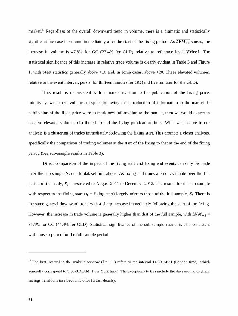
market.17

Regardless of the overall downward trend in volume, there is a dramatic and statistically

significant increase in volume immediately after the start of the fixing period. As ∆𝑽𝑴+𝟏 shows, the

increase in volume is 47.8% for GC (27.4% for GLD) relative to reference level, 𝐕𝐌𝐫𝐞𝐟 . The

statistical significance of this increase in relative trade volume is clearly evident in Table 3 and Figure

1, with t-test statistics generally above +10 and, in some cases, above +20. These elevated volumes,

relative to the event interval, persist for thirteen minutes for GC (and five minutes for the GLD).

This result is inconsistent with a market reaction to the publication of the fixing price.

Intuitively, we expect volumes to spike following the introduction of information to the market. If

publication of the fixed price were to mark new information to the market, then we would expect to

observe elevated volumes distributed around the fixing publication times. What we observe in our

analysis is a clustering of trades immediately following the fixing start. This prompts a closer analysis,

specifically the comparison of trading volumes at the start of the fixing to that at the end of the fixing

period (See sub-sample results in Table 3).

Direct comparison of the impact of the fixing start and fixing end events can only be made

over the sub-sample Ss due to dataset limitations. As fixing end times are not available over the full

period of the study, Ss is restricted to August 2011 to December 2012. The results for the sub-sample

with respect to the fixing start (t0 = fixing start) largely mirrors those of the full sample, Sf. There is

the same general downward trend with a sharp increase immediately following the start of the fixing.

However, the increase in trade volume is generally higher than that of the full sample, with ∆𝑽𝑴+𝟏 =

81.1% for GC (44.4% for GLD). Statistical significance of the sub-sample results is also consistent

with those reported for the full sample period.

17 The first interval in the analysis window (i = -29) refers to the interval 14:30-14:31 (London time), which

generally correspond to 9:30-9:31AM (New York time). The exceptions to this include the days around daylight

savings transitions (see Section 3.6 for further details).

22

To analyse the impact of the fixing end on trade volume, the event period is set to the one

minute interval immediately following the fixing publication time. As the fixing duration varies this

does not correspond to a constant time of day, unlike the fixing start. Our results from this analysis are

also reported in Table 3. Similar to the results for the fixing start, there is the same general downward

trend in volume. However, there is no corresponding spike in volume around the publication of the

fixing result. For GC, the peak in trade volumes is found around four minutes before the end of the

fixing, though this is not a statistically significant increase relative to the fixing end interval. The

results for GLD are similar: volume peaks five minutes before the end of the fix, with both i = -5 and i

= -4 showing volumes significantly higher than the event interval. In both cases, the volume spike

occurs at the start of the fixing convolved with the distribution of the fixing durations. Apart from

these spikes, there are no other intervals that show a significant difference in volume until five minutes

after the fix end (i = 4). Again, differences in subsequent intervals (i ≥ 4) are attributed to a general

down trend, rather than any discernible volume spike.

In summary, trade volumes in GC and GLD exhibit a large, statistically significant spike

immediately after the start of the fixing. This elevated level of trade activity impacts GC more than

GLD, and also lasts longer for GC. Furthermore, there is no significant change in trade volume aligned

with the end of the fixing.

4.2 Relative volatility

The results from our analysis of relative price volatility around the time of the London PM

gold fixing are reported in Table 4 for both GC and GLD, and these largely follow the previous results

on trade volume. The analysis is based on one minute interval volatility estimates, which are

calculated using the Garman-Klass volatility estimator given high, low, open and close prices for each

one-minute interval. Separate results are reported for both GC and GLD, as well as for the following

sample periods: the full sample period Sf , with t0 = the fixing start; the sub-sample period Ss, with t0 =

the fixing start; and Ss with t0 = the fixing end. Each of the three sets of results refer to average

23

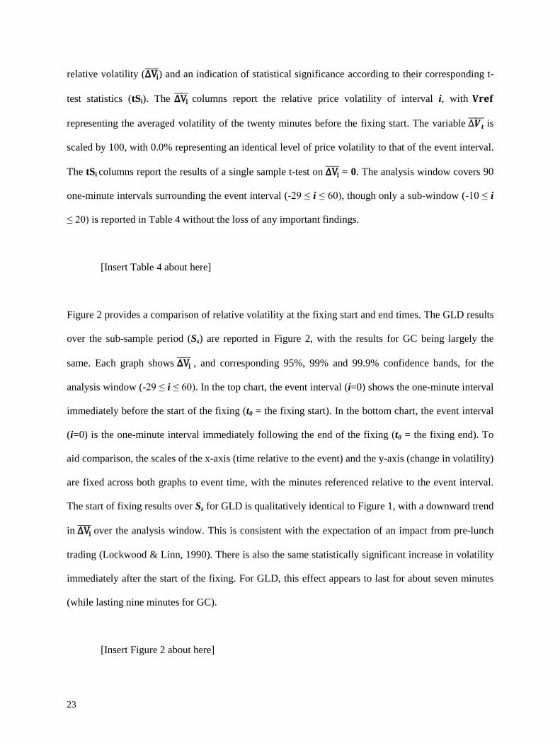
relative volatility (∆Vi ) and an indication of statistical significance according to their corresponding t-

test statistics (tSi). The ∆Vi columns report the relative price volatility of interval i, with 𝐕𝐫𝐞𝐟

representing the averaged volatility of the twenty minutes before the fixing start. The variable ∆𝑽𝒊 is

scaled by 100, with 0.0% representing an identical level of price volatility to that of the event interval.

The tSi columns report the results of a single sample t-test on ∆Vi = 0. The analysis window covers 90

one-minute intervals surrounding the event interval (-29 ≤ i ≤ 60), though only a sub-window (-10 ≤ i

≤ 20) is reported in Table 4 without the loss of any important findings.

[Insert Table 4 about here]

Figure 2 provides a comparison of relative volatility at the fixing start and end times. The GLD results

over the sub-sample period (Ss) are reported in Figure 2, with the results for GC being largely the

same. Each graph shows ∆Vi , and corresponding 95%, 99% and 99.9% confidence bands, for the

analysis window (-29 ≤ i ≤ 60). In the top chart, the event interval (i=0) shows the one-minute interval

immediately before the start of the fixing (t0 = the fixing start). In the bottom chart, the event interval

(i=0) is the one-minute interval immediately following the end of the fixing (t0 = the fixing end). To

aid comparison, the scales of the x-axis (time relative to the event) and the y-axis (change in volatility)

are fixed across both graphs to event time, with the minutes referenced relative to the event interval.

The start of fixing results over Ss for GLD is qualitatively identical to Figure 1, with a downward trend

in ∆Vi over the analysis window. This is consistent with the expectation of an impact from pre-lunch

trading (Lockwood & Linn, 1990). There is also the same statistically significant increase in volatility

immediately after the start of the fixing. For GLD, this effect appears to last for about seven minutes

(while lasting nine minutes for GC).

[Insert Figure 2 about here]

24

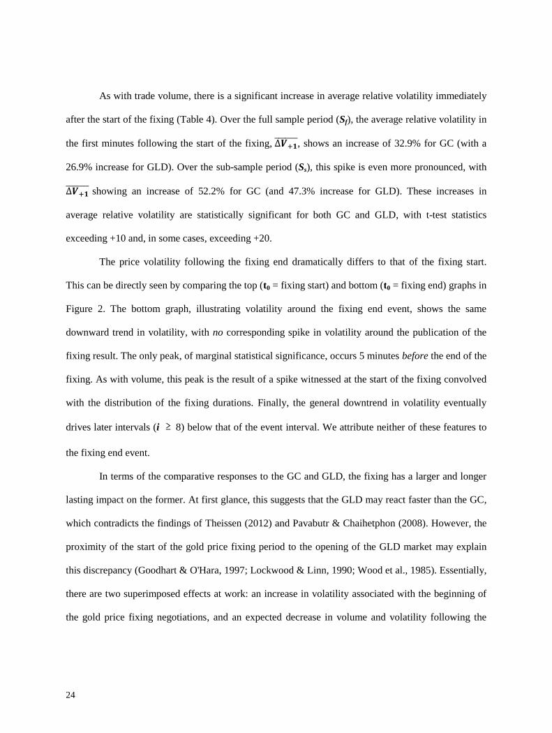
As with trade volume, there is a significant increase in average relative volatility immediately

after the start of the fixing (Table 4). Over the full sample period (Sf), the average relative volatility in

the first minutes following the start of the fixing, ∆𝑽+𝟏 , shows an increase of 32.9% for GC (with a

26.9% increase for GLD). Over the sub-sample period (Ss), this spike is even more pronounced, with

∆𝑽+𝟏 showing an increase of 52.2% for GC (and 47.3% increase for GLD). These increases in

average relative volatility are statistically significant for both GC and GLD, with t-test statistics

exceeding +10 and, in some cases, exceeding +20.

The price volatility following the fixing end dramatically differs to that of the fixing start.

This can be directly seen by comparing the top (t0 = fixing start) and bottom (t0 = fixing end) graphs in

Figure 2. The bottom graph, illustrating volatility around the fixing end event, shows the same

downward trend in volatility, with no corresponding spike in volatility around the publication of the

fixing result. The only peak, of marginal statistical significance, occurs 5 minutes before the end of the

fixing. As with volume, this peak is the result of a spike witnessed at the start of the fixing convolved

with the distribution of the fixing durations. Finally, the general downtrend in volatility eventually

drives later intervals (i ≥ 8) below that of the event interval. We attribute neither of these features to

the fixing end event.

In terms of the comparative responses to the GC and GLD, the fixing has a larger and longer

lasting impact on the former. At first glance, this suggests that the GLD may react faster than the GC,

which contradicts the findings of Theissen (2012) and Pavabutr & Chaihetphon (2008). However, the

proximity of the start of the gold price fixing period to the opening of the GLD market may explain

this discrepancy (Goodhart & O'Hara, 1997; Lockwood & Linn, 1990; Wood et al., 1985). Essentially,

there are two superimposed effects at work: an increase in volatility associated with the beginning of

the gold price fixing negotiations, and an expected decrease in volume and volatility following the

25

market opening. While we do not attempt to disentangle these two effects, it should caution against

any simple comparisons of the GC and the GLD results.

In summary, GC and GLD both exhibit large, statistically significant spikes in price volatility

immediately following the start of the fixing. This elevated level of price volatility impacts GC

slightly more than GLD, and persists longer for GC. Further, there is no significant change in volatility

aligned with the end of the fixing. As argued in the trade volume analysis, increased volatility is not

expected until after the publication of the fixing result (fixing end). This coincides with our findings

from the trade volume analysis (that is, the fixing does have an impact on the exchange-traded markets)

and, further, suggests that information may be leaking from the fixing process ahead of the publication

of the fixing result. This result is robust to the choice of volatility estimator; similar results are

obtained using the Parkinson and the Rogers-Satchell estimators in place of the Garman-Klass

estimator.

4.3 Returns

Tables 5, 6 and 7 report results from our analysis on unadjusted returns, adjusted returns and

the difference between these returns, respectively. The unadjusted returns reflect an uninformed long

position in either GLD or GC, and the adjusted returns represent an informed position depending on

the price direction signalled by the final fixed price. To realise these adjusted returns, a trader would

require directional foresight on price. Finally, the difference in returns reflects simply the difference

between the adjusted and unadjusted returns, which quantifies the value of the directional foresight to

an informed trader.

[Insert Tables 5, 6 and 7 about here]

The above tables include results for both the GC and GLD datasets, with the three sets

covering the full sample period Sf with t0 = the fixing start, the sub-sample period Ss with t0 = the

26

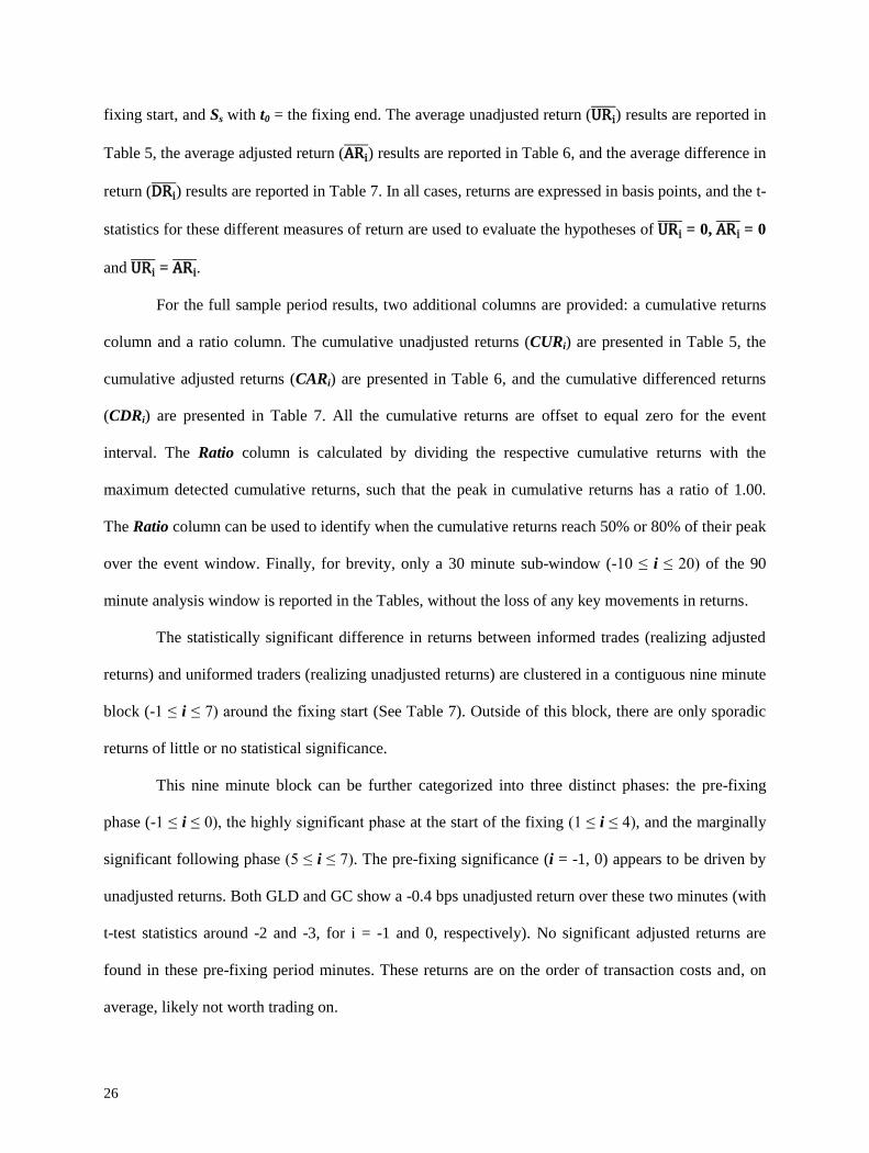
fixing start, and Ss with t0 = the fixing end. The average unadjusted return (URi ) results are reported in

Table 5, the average adjusted return (ARi ) results are reported in Table 6, and the average difference in

return (DRi ) results are reported in Table 7. In all cases, returns are expressed in basis points, and the t-

statistics for these different measures of return are used to evaluate the hypotheses of URi = 0, ARi

= 0

and URi = ARi

.

For the full sample period results, two additional columns are provided: a cumulative returns

column and a ratio column. The cumulative unadjusted returns (CURi) are presented in Table 5, the

cumulative adjusted returns (CARi) are presented in Table 6, and the cumulative differenced returns

(CDRi) are presented in Table 7. All the cumulative returns are offset to equal zero for the event

interval. The Ratio column is calculated by dividing the respective cumulative returns with the

maximum detected cumulative returns, such that the peak in cumulative returns has a ratio of 1.00.

The Ratio column can be used to identify when the cumulative returns reach 50% or 80% of their peak

over the event window. Finally, for brevity, only a 30 minute sub-window (-10 ≤ i ≤ 20) of the 90

minute analysis window is reported in the Tables, without the loss of any key movements in returns.

The statistically significant difference in returns between informed trades (realizing adjusted

returns) and uniformed traders (realizing unadjusted returns) are clustered in a contiguous nine minute

block (-1 ≤ i ≤ 7) around the fixing start (See Table 7). Outside of this block, there are only sporadic

returns of little or no statistical significance.

This nine minute block can be further categorized into three distinct phases: the pre-fixing

phase (-1 ≤ i ≤ 0), the highly significant phase at the start of the fixing (1 ≤ i ≤ 4), and the marginally

significant following phase (5 ≤ i ≤ 7). The pre-fixing significance (i = -1, 0) appears to be driven by

unadjusted returns. Both GLD and GC show a -0.4 bps unadjusted return over these two minutes (with

t-test statistics around -2 and -3, for i = -1 and 0, respectively). No significant adjusted returns are

found in these pre-fixing period minutes. These returns are on the order of transaction costs and, on

average, likely not worth trading on.

27

Once the fixing starts, the results are far more dramatic, with the initial four minutes (1 ≤ i ≤ 4)

showing the difference in returns of +3.8 bps, +3.0 bps, +1.8 bps and +1.0 bps for GC, and +3.8 bps,

+3.2 bps, +1.7 bps and +1.1 bps for GLD. The significance of these four minutes by far exceeds that

of any other period in our analysis; the t-test statistics associated with these average returns range from

over +17 for DR+1 , down to +7.2 for DR+4

. Unlike the two pre-fixing intervals, these results are

primarily driven by adjusted returns, while the unadjusted returns in the first two minutes of the fixing

are smaller and show far lower statistical significance. Using GC as an example, UR+1 = -0.6 bps (tS+1

= -3.3) and UR+2 = -1.2 bps (tS+2 = -6.7), while AR+1

= -3.1 bps (tS+1 = +17.6) and AR+2 = -1.8 bps

(tS+2 = +10.5). The subsequent two minutes (i = 3, 4) show no significant unadjusted returns, while

adjusted returns remain above 1.0 bps with t-test statistics above +7.

Four minutes after the fixing start, our results show only marginal significance of returns. For

the fifth minute into the fixing (i = 5), there is no significant difference in adjusted and unadjusted

returns. Curiously, this is attributed to both unadjusted and adjusted returns being approximately +0.5

bps. The last two minutes of the nine minute block (i = 6, 7) show some difference in returns, albeit

small and at weaker levels of significance. These are driven solely by the adjusted returns, with

unadjusted returns showing no significance.

Figure 3 provides a composite of four charts, featuring (from top to bottom): the GLD average

adjusted returns (ARi ) over the full sample period; the GLD cumulative average adjusted returns

(CARi); the distribution histogram of GLD adjusted returns (ARi) immediately before the start of the

fixing; and the distribution histogram of GLD adjusted returns immediately after the start of the fixing.

[Insert Figure 3 about here]

The ARi chart illustrates two key findings. First, the relative size and significance of returns in

the analysis window are generally insignificant, with the exception of a seven minute block following

28

the fixing start. Second, adjusted returns are greatest and most statistically significant immediately

following the start of the fixing. The CARi plot illustrates that the cumulative effects of the adjusted

returns are not only statistically significant, but are also profitable for those with knowledge of the

direction of the fixed price relative to the current price. The cumulative returns are also close to zero

for most of the period prior to the start of the fixing period, and when the fixing starts, adjusted returns

jump dramatically. Around 50% of this jump is realized within the first two minutes of the fixing,

while 80% is realised within the first five minutes. The cumulative returns peak at approximately 12

minutes from the start of the fixing (i=12). The subsequent hour of returns show little change in the

CAR. Similar to the results for relative volume and volatility, the bottom pair of histograms illustrate

that there is a marked right-shift in the distribution of adjusted returns immediately before and after

the start.

These results are not driven by any secular trend over the sample period. While there was a

secular bull market in gold for much of the period, up to September 2011, the fixing directions

(FIXDIRd) are relatively evenly distributed. For GC (GLD), there are 770 (754) up days, 708 (691)

down days and 26 (25) flat days. Analysis of the returns on up and down days yields largely similar

results, with the up days showing somewhat larger adjusted returns.

This result is critically important; it shows that the higher volume and volatility immediately

following the fix start is not just uninformed speculation. If it were, the exchange-traded contract

prices would move in the opposite direction to that implied by the upcoming fix as often as they move

in the same direction. Returns would balance and there would be no discernible increase in the CAR.

Instead, we see a very coherent increase aligned to the fixing start.

Analysis of the sub-period provides additional insight into the contrast between the fixing start

and the fixing end. These results are also reported in Tables 5, 6 and 7. While significant differences in

returns are more concentrated in time, evident only in the first two minutes following the start of the

fixing. The effect is of similar magnitude to the full period analysis in which DR+1 = +4.2 bps (+4.1

29

bps) and DR+2 = +4.2 bps (+4.4 bps) for GC (GLD). The significance of these returns is supported by

t-test statistics that exceed +5. A cumulative difference in returns of around +8.5bps within the

opening two minutes suggests that participants are reacting more quickly in recent years relative to the

full sample period. The difference in returns is largely driven by adjusted returns.

There are also statistically significant difference in returns within the last three minutes of the

fixing, in which DR-2 = -0.9bps (-1.1bps), DR-1

= -1.5 bps (-1.5 bps), and DR0 = -1.2 bps (-1.4 bps) for

GC (GLD). These returns are of particular interest as they exhibit the opposite signs to the difference

in returns reported at the start of the fixing period. While the DR-2 is only marginally significant, tS-2

= -2.2 (-2.4) for GC (GLD), the intervals closer to the end of the fixing (i = -1, 0), the magnitude of the

t-test statistic is approximately -4. The total difference in returns over these three closing minutes of

the fixing is -3.8 bps (-4.0 bps) for GC (GLD).

These return dynamics are best illustrated in Figure 4, where the adjusted returns for both the

start of the fix and the end of the fix are shown for GC. Both the interval returns and the cumulative

returns are indicated. The cumulative returns highlight the effect of the value to an informed trader of

taking positions in the contract with reference to the fixed price. These returns are present only after

the start of the fixing and before its end.

[Insert Figure 4 about here]

Note the decline in the CAR when viewed from the end of the fixing, as shown in the bottom

right chart in Figure 4, which appears to be driven by the fixing end. However, this is merely an

artefact of the prior run-up in the CAR, from the fixing start, and the offset from the definition of CAR,

(that is, CAR at i = 0 is defined to be zero). Given that, the two minutes leading to the end of the

fixing do show statistically significant negative returns. One possible explanation for this is the

overshoot caused by uniformed traders. It is possible (and likely) that uninformed participants ‘piggy-

30

back’ on the price movements established from the fixing start. That is, having observed trades move

in a certain direction following the fixing start, the uninformed trader places similar directional bets.

This in turn can cause the instruments to overshoot the final fixing price. As the fixing draws to an end,

and the final price becomes known to the fixing participants, this overshoot in price provides the

informed traders an additional profit opportunity. To realize this, the informed trader must reverse

their initial position. This would explain both the timing and inverted sign of the adjusted returns at

the end of the fixing. Further analysis of this possibility is beyond the scope of the present study.

In summary, the empirical analysis suggests that an informed trader, with directional foresight

of the fixing price, can earn returns in excess of those available to an uninformed trader. These returns

are realizable largely in the four minutes following the start of the fixing. The excess returns are on the

order of 10 bps and are statistically significant for both GC and GLD. A further, albeit smaller and less

certain, trading edge of about 4 bps appears to be available in the two minutes before the end of the

fixing. The excess returns following the start, and just before the end, of the fixing are above the 3 bps

that traders would reasonably expect to face when trading in these markets.18

4.4 Predictive value of market returns

The results of the analysis on comparative predictive power of market price movements are

given in Table 8. The table reports the findings for the first twelve cut-off times after the start of the

fixing (1 ≤ 𝑖 ≤ 12), as well as the interval before the start of the fixing (𝑖 = 0). For each cut-off

time i, a sub-sample of fixings (Si) with durations longer than i minutes is selected. Each sub-sample

Si is further divided into big (Si,big) and small (Si,sml) sub-sets based on the magnitude of each fixing

price change (FIXMAG). The table presents the summary statistics and prediction statistics for Si, Si,big

and Si,sml in relation to the GC, though similar results were found for the GLD.

18 While not presented, this analysis was also conducted on the physical spot gold (XAU=) and yields largely

similar results.

31

[Insert Table 8 about here]

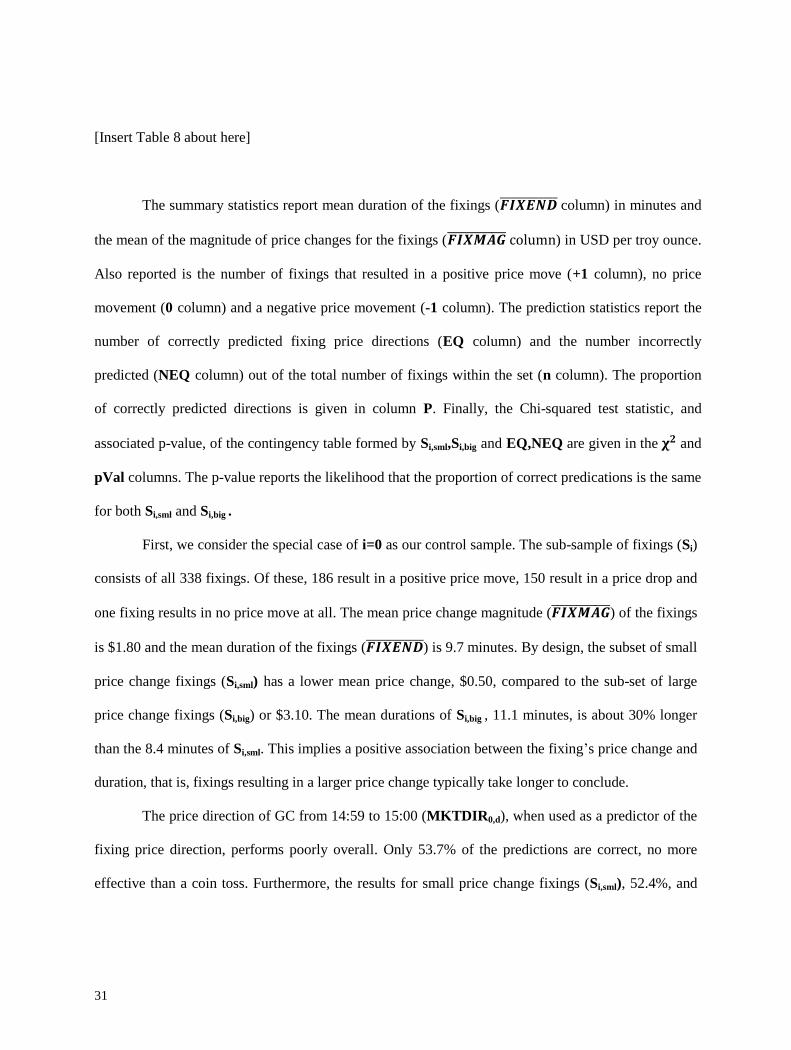
The summary statistics report mean duration of the fixings (𝑭𝑰𝑿𝑬𝑵𝑫 column) in minutes and

the mean of the magnitude of price changes for the fixings (𝑭𝑰𝑿𝑴𝑨𝑮 column) in USD per troy ounce.

Also reported is the number of fixings that resulted in a positive price move (+1 column), no price

movement (0 column) and a negative price movement (-1 column). The prediction statistics report the

number of correctly predicted fixing price directions (EQ column) and the number incorrectly

predicted (NEQ column) out of the total number of fixings within the set (n column). The proportion

of correctly predicted directions is given in column P. Finally, the Chi-squared test statistic, and

associated p-value, of the contingency table formed by Si,sml,Si,big and EQ,NEQ are given in the 𝛘𝟐 and

pVal columns. The p-value reports the likelihood that the proportion of correct predications is the same

for both Si,sml and Si,big .

First, we consider the special case of i=0 as our control sample. The sub-sample of fixings (Si)

consists of all 338 fixings. Of these, 186 result in a positive price move, 150 result in a price drop and

one fixing results in no price move at all. The mean price change magnitude (𝑭𝑰𝑿𝑴𝑨𝑮 ) of the fixings

is $1.80 and the mean duration of the fixings (𝑭𝑰𝑿𝑬𝑵𝑫 ) is 9.7 minutes. By design, the subset of small

price change fixings (Si,sml) has a lower mean price change, $0.50, compared to the sub-set of large

price change fixings (Si,big) or $3.10. The mean durations of Si,big , 11.1 minutes, is about 30% longer

than the 8.4 minutes of Si,sml. This implies a positive association between the fixing’s price change and

duration, that is, fixings resulting in a larger price change typically take longer to conclude.

The price direction of GC from 14:59 to 15:00 (MKTDIR0,d), when used as a predictor of the

fixing price direction, performs poorly overall. Only 53.7% of the predictions are correct, no more

effective than a coin toss. Furthermore, the results for small price change fixings (Si,sml), 52.4%, and

32

large price change fixings (Si,big), 55.0%, are statistically indistinguishable. The Chi-square statistic of

0.2 implies a p-value of 0.626.

Now consider the cases in which i > 1. What separates these cases from the i = 0 case above is

the inclusion of price movements after the start of the fixings. In the case of i = 1, the predictor

(MKTDIRi,d) is derived from the price direction of GC from 15:00 to 15:01. The sub-sample of

fixings (Si) consists of the 320 fixings that were reported at 15:02 or later. While the summary

statistics remain largely the same, the prediction statistics show a dramatic change. Not only has the

overall prediction rate increased to around 70%, the predictions for Si,big are almost 80% correct,

compared with a little more than 60% for Si,sml. The likelihood that large and small price change

fixings have the same prediction rates is rejected at the 0.1% significance level, with a Chi-square

statistic of 11.4.

The results become increasingly stark over the next handful of minutes, peaking at i = 6. Here,

the predictor is derived from the price direction of GC from 15:00 to 15:06, with the sub-sample of

fixings (Si) consists of the 205 fixings that were reported at 15:07 or later. The overall correct

prediction rate is nearly 80%. For Si,big, it is above 95% while for Si,sml, it remains around 60%

(yielding a Chi-square statistic over 30). The price direction of 98 of the 103 fixings in Si,big were

correctly predicted at least one minute, and on average 5.4 minutes, before the publication of the

fixing price by observing the price movement of the GC contract from 15:00 to 15:06.

In summary, the analysis finds that not only are the price movements of the publicly-traded

instruments predictive of the fixing price direction, they are significantly more predictive for the

fixings that result in large price changes. That is, not only are the trades quite accurate in predicting

the fixing direction, the more money that is made by way of a larger price change, the more accurate

the trade becomes. This is highly suggestive of information leaking from the fixing to these public

markets.

33

5.0 Conclusion

There are two questions that this paper seeks to address concerning the interaction between the

public, central exchange-based gold instrument markets and the relatively closed, opaque London gold

fixing mechanism. First, does the London PM fixing, used as a mechanism for price determination in

the wholesale physical market, have an impact on the dynamics of exchange traded instruments?

Second, does information from the fixing leak into the public markets prior to the publication of the

fixing result, which could possibly grant a trade advantage to participants privy to the price fixing

process? The analysis focuses on two of the most active exchange-traded gold instruments, the GC

and the GLD, in order to address these questions.

In addressing the first question, it is evident that both the GC and GLD markets are

significantly impacted by the London PM gold price fixing process. Both instruments exhibit large,

statistically significant spikes in trade volume and price volatility immediately following the start of

the fixing. Trade volumes increase over 50%, while price volatility increases over 40% following the

fixing start. However, there is no evidence of a significant change in either price volatility or trade

volume following the end of the fixing.

In addressing the second question, this study finds evidence of information leaking from the

London PM gold price fixing into the GC and GLD markets prior to the publication of the fixing result.

This extends beyond the elevated market activity found at the start of the fixing period. There is also

evidence of statistically significant differences in the returns that could be earned by informed versus

uninformed participants. These are clustered immediately following the start and just before the end of

the fixing. The difference in returns suggests an informed trader has an advantage of around 10 bps in

the first four minutes following the start of the fixing, and a possible further 4 bps in the two minutes

before the end of the fixing. These returns exceed trading costs and are deemed economic. There is no

evidence of statistically significant returns or elevated levels of trade activity following the publication

of the fixing result. The degree to which participants are directionally informed and, critically, how

34

quickly they become informed limits their ability to capture this advantage. The predictability of the

fixing direction further suggests that fixing participants become informed within the first minutes of

the fixing. Trades are found to be highly predictive of the fixing price direction, especially when the

fixings result in large price movements. These results are evident in both the GC and GLD markets.

While we have not presented results for the AM fixing, preliminary analysis suggests qualitatively

similar results for the GC.

These findings might give cause for concern, both for regulators and broader market

participants. They also provide some support for the calls for a review of the London gold fixing

mechanism.19

For regulators, given the current tide of financial regulatory reform, triggered in no

small part by the current LIBOR scandal, this examination of the gold fixing is timely. The possibility

of problems also existing with the OTC commodity market has been noted. For example, in a recent

Bloomberg article about the problems with LIBOR, the FSA Managing Director, Martin Wheatley,

made the comment that “other benchmarks, such as for the prices of agricultural products, oil and

precious metals, and in the equity, bond and money markets, should be looked at as well”.20

Enhancing transparency may be all that is needed to address the issues raised in this study.

Measures could range from enabling access to the audio stream form the fixing to running the auction

through a public electronic limit order book. This would maintain the existing structures, including the

client’s need for anonymity, while removing the information advantage that accrues to fixing

participants. A more sweeping reform could include moving the fixing to a more formal exchange

where all participants stand equally — effectively abolishing the fixing altogether. However, this more

heavy-handed approach could ultimately prove counterproductive should wholesale market

19March 14, 2013. (http://uk.reuters.com/article/2013/03/13/uk-gold-cftc-probe-

idUKBRE92C11020130313?type=GCA-ForeignExchange).

20 September 28, 2012 (http://www.bloomberg.com/news/2012-09-27/fsa-to-oversee-libor-in-streamlining-of-

tarnished-rates.html).

35

participants withdraw from the process completely only to reconvene informally in an even less

regulated market.

The fixing has over the course of the past century demonstrated both adaptability and

resilience in the face dramatic market changes. The broad suspension of gold convertibility in the

wake of the world wars, the reintroduction of U.S. dollar convertibility under the Bretton Woods

agreement, and it’s subsequent collapse. In this context, the current tide of regulatory overhauls can be

viewed as a relatively minor, and potentially quite constructive.

Possible extensions to this work include extending the analysis to include a greater range of

available derivative contracts, including options and futures contracts, as well as a wider range of the

ETFs that focus on gold. It is also possible to extend the analysis to include the AM fixing and its

impact on European exchange-based markets. Finally, analysing other commodities with similar price

setting arrangements, such as silver, may provide interesting insights — particularly as the close

relationship between the two precious metals yields the possibility of interactions across their

respective fixings. We leave these issues to future research.

36

6.0 References

Abken, P., A. (1980). The economics of gold price movements. Federal Reserve Bank of

Richmond Economic Review, 66(2), 3-13.

Aggarwal, R., & Lucey, B. M. (2007). Psychological barriers in gold prices? Review of

Financial Economics, 16(2), 217-230.

Ashish, B., Dempster, N., & Milling-Stanley, G. (2011). Liquidity in the Global Gold Market.

Basu, S., & Clouse, M. L. (1993). A comparative analysis of gold market efficiency using

derivative market information. Resources Policy, 19(3), 217-224.

Beckers, S. (1984). On the efficiency of the gold options market. Journal of Banking &

Finance, 8(3), 459-470.

Blose, L. E. (2009). Gold prices, cost of carry, and expected inflation. Journal of Economics

and Business, 62(1), 35-47.

Charupat, N., & Miu, P. (2011). The pricing and performance of leveraged exchange-traded

funds. Journal of Banking & Finance, 35(4), 966-977.

Chng, M. T. (2009). Economic linkages across commodity futures: Hedging and trading

implications. Journal of Banking & Finance, 33(5), 958-970.

Christie–David, R., Chaudhry, M., & Koch, T. W. (2000). Do macroeconomics news releases

affect gold and silver prices? Journal of Economics and Business, 52(5), 405-421.

Dwyer, A., Gardner, George and Williams, Thomas (2011). Global Commodity Markets –

Price Volatility and Financialisation. RBA Bulletin(June Quarter), 9.

Ederington, L. H., & Lee, J. H. (1995). The Short-Run Dynamics of the Price Adjustment to

New Information. Journal of Financial and Quantitative Analysis, 30(1), 117-134.

Followill, R. A., & Helms, B. P. (1990). Put-call-futures parity and arbitrage opportunity in

the market for options on gold futures contracts. Journal of Futures Markets, 10(4),

339-352.

Goodhart, C. A. E., & O'Hara, M. (1997). High frequency data in financial markets: Issues

and applications. Journal of Empirical Finance, 4(2–3), 73-114.

Levin, E. J., Montagnoli, A. and Wright, R.E. (2006). Short-run and long-run determinants of

the price of gold (Report): World Gold Council.

Lockwood, L. J., & Linn, S. C. (1990). An Examination of Stock Market Return Volatility

During Overnight and Intraday Periods, 1964–1989. The Journal of Finance, 45(2),

591-601.

Narayan, P. K., Narayan, S., & Zheng, X. (2010). Gold and oil futures markets: Are markets

efficient? Applied Energy, 87(10), 3299-3303.

O`Callaghan, G. (1991). The Structure and Operation of the World Gold Market. IMF

Working Paper, 91(120).

Pavabutr, P., & Chaihetphon, P. (2008). Price discovery in the Indian gold futures market.

Journal of Economics and Finance, 34(4), 455-467.

Theissen, E. (2012). Price discovery in spot and futures markets: a reconsideration. The

European Journal of Finance, 18(10), 969-987.

Tschoegl, A. E. (1980). Efficiency in the gold market — a note. Journal of Banking &

Finance, 4(4), 371-379.

Wood, R. A., McInish, T. H., & Ord, J. K. (1985). An Investigation of Transactions Data for

NYSE Stocks. The Journal of Finance, 40(3), 723-739.

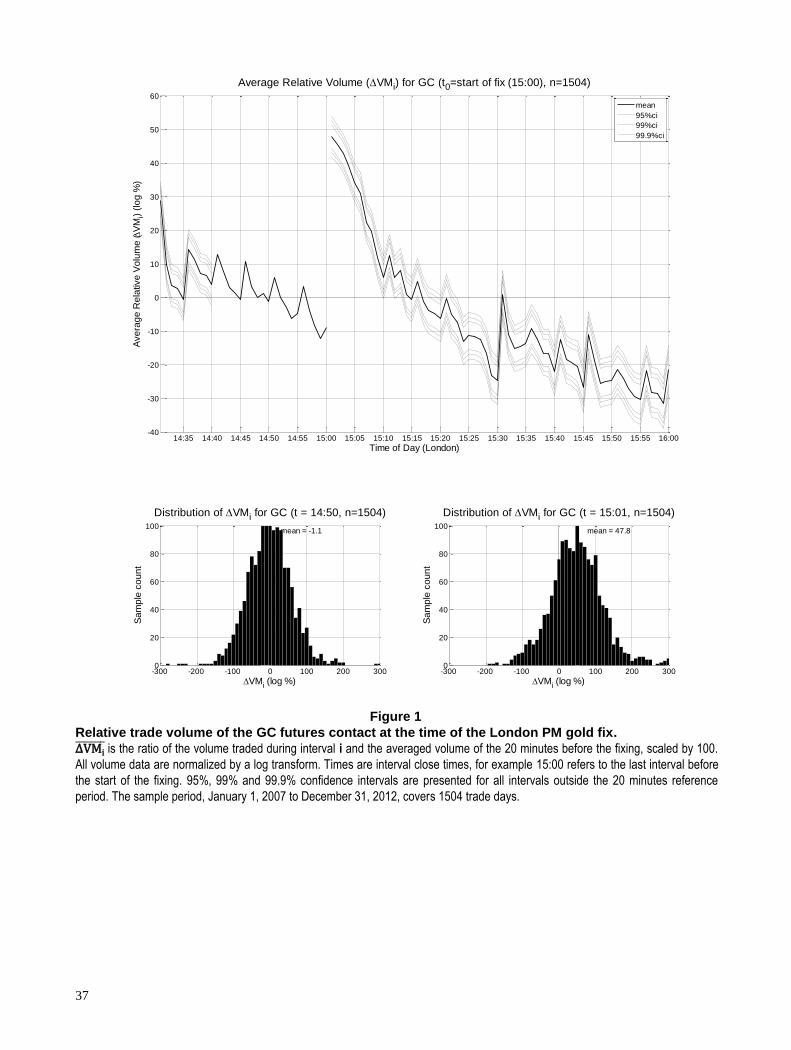
37

Figure 1

Relative trade volume of the GC futures contact at the time of the London PM gold fix.

∆VMi is the ratio of the volume traded during interval i and the averaged volume of the 20 minutes before the fixing, scaled by 100.

All volume data are normalized by a log transform. Times are interval close times, for example 15:00 refers to the last interval before

the start of the fixing. 95%, 99% and 99.9% confidence intervals are presented for all intervals outside the 20 minutes reference

period. The sample period, January 1, 2007 to December 31, 2012, covers 1504 trade days.

14:35 14:40 14:45 14:50 14:55 15:00 15:05 15:10 15:15 15:20 15:25 15:30 15:35 15:40 15:45 15:50 15:55 16:00-40

-30

-20

-10

0

10

20

30

40

50

60

Time of Day (London)

Ave

rag

e R

ela

tive

Vo

lum

e (

VM

i) (

log

%)

Average Relative Volume (VMi) for GC (t0=start of fix (15:00), n=1504)

mean

95%ci

99%ci

99.9%ci

-300 -200 -100 0 100 200 3000

20

40

60

80

100

Distribution of VMi for GC (t = 14:50, n=1504)

VMi (log %)

Sa

mp

le c

ou

nt

mean = -1.1

-300 -200 -100 0 100 200 3000

20

40

60

80

100

Distribution of VMi for GC (t = 15:01, n=1504)

VMi (log %)

Sa

mp

le c

ou

nt

mean = 47.8

-300 -200 -100 0 100 200 3000

20

40

60

80

100

Distribution of VMi for GC (t = 14:58, n=1504)

VMi (log %)

Sa

mp

le c

ou

nt

mean = -8.3

-300 -200 -100 0 100 200 3000

20

40

60

80

100

Distribution of VMi for GC (t = 15:02, n=1504)

VMi (log %)

Sa

mp

le c

ou

nt

mean = 45.4

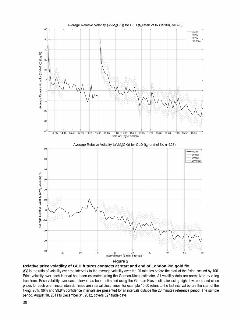
38

Figure 2

Relative price volatility of GLD futures contacts at start and end of London PM gold fix.

∆Vi is the ratio of volatility over the interval i to the average volatility over the 20 minutes before the start of the fixing, scaled by 100.

Price volatility over each interval has been estimated using the Garman-Klass estimator. All volatility data are normalized by a log

transform. Price volatility over each interval has been estimated using the Garman-Klass estimator using high, low, open and close

prices for each one minute interval. Times are interval close times, for example 15:00 refers to the last interval before the start of the

fixing. 95%, 99% and 99.9% confidence intervals are presented for all intervals outside the 20 minutes reference period. The sample

period, August 18, 2011 to December 31, 2012, covers 327 trade days.

14:35 14:40 14:45 14:50 14:55 15:00 15:05 15:10 15:15 15:20 15:25 15:30 15:35 15:40 15:45 15:50 15:55-40

-30

-20

-10

0

10

20

30

40

50

60

Time of Day (London)

Ave

rag

e R

ela

tive

Vo

latilty (

VM

i(G

K))

(lo

g %

)

Average Relative Volatilty (VMi(GK)) for GLD (t0=start of fix (15:00), n=328)

mean

95%ci

99%ci

99.9%ci

-20 -10 0 10 20 30 40 50 60-40

-30

-20

-10

0

10

20

30

40

50

60

Average Relative Volatilty (VMi(GK)) for GLD (t0=end of fix, n=328)

Interval index (1 min. intervals)

Ave

rag

e R

ela

tive

Vo

latilty (

VM

i(G

K))

(lo

g %

)

mean

95%ci

99%ci

99.9%ci

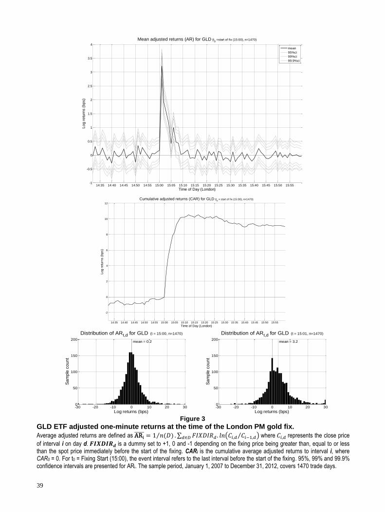
39

Figure 3

GLD ETF adjusted one-minute returns at the time of the London PM gold fix.

Average adjusted returns are defined as ARi = 1 𝑛(𝐷)⁄ . ∑ 𝐹𝐼𝑋𝐷𝐼𝑅𝑑 . 𝑙𝑛(𝐶𝑖,𝑑 𝐶𝑖−1,𝑑⁄ )𝑑∈𝐷 where 𝐶𝑖,𝑑 represents the close price

of interval i on day d. 𝑭𝑰𝑿𝑫𝑰𝑹𝒅 is a dummy set to +1, 0 and -1 depending on the fixing price being greater than, equal to or less than the spot price immediately before the start of the fixing. CARi is the cumulative average adjusted returns to interval i, where CAR0 = 0. For t0 = Fixing Start (15:00), the event interval refers to the last interval before the start of the fixing. 95%, 99% and 99.9% confidence intervals are presented for ARi. The sample period, January 1, 2007 to December 31, 2012, covers 1470 trade days.

14:35 14:40 14:45 14:50 14:55 15:00 15:05 15:10 15:15 15:20 15:25 15:30 15:35 15:40 15:45 15:50 15:55-1

-0.5

0

0.5

1

1.5

2

2.5

3

3.5

4

Time of Day (London)

Lo

g r

etu

rns (

bp

s)

Mean adjusted returns (AR) for GLD (t0 =start of fix (15:00), n=1470)

mean

95%ci

99%ci

99.9%ci

14:35 14:40 14:45 14:50 14:55 15:00 15:05 15:10 15:15 15:20 15:25 15:30 15:35 15:40 15:45 15:50 15:55

-2

0

2

4

6

8

10

12

Time of Day (London)

Lo

g r

etu

rns (

bp

s)

Cumulative adjusted returns (CAR) for GLD (t0 = start of fix (15:00), n=1470)

-30 -20 -10 0 10 20 300

50

100

150

200

Distribution of ARt,d for GLD (t = 15:00, n=1470)

Log returns (bps)

Sa

mp

le c

ou

nt

mean = 0.2

-30 -20 -10 0 10 20 300

50

100

150

200

Distribution of ARt,d for GLD (t = 15:01, n=1470)

Log returns (bps)

Sa

mp

le c

ou

nt

mean = 3.2

-30 -20 -10 0 10 20 300

50

100

150

200

Distribution of ARt,d for GLD (t = 15:02, n=1470)

Log returns (bps)

Sa

mp

le c

ou

nt

mean = 1.9

-30 -20 -10 0 10 20 300

50

100

150

200

Distribution of ARt,d for GLD (t = 15:03, n=1470)

Log returns (bps)

Sa

mp

le c

ou

nt

mean = 1.5

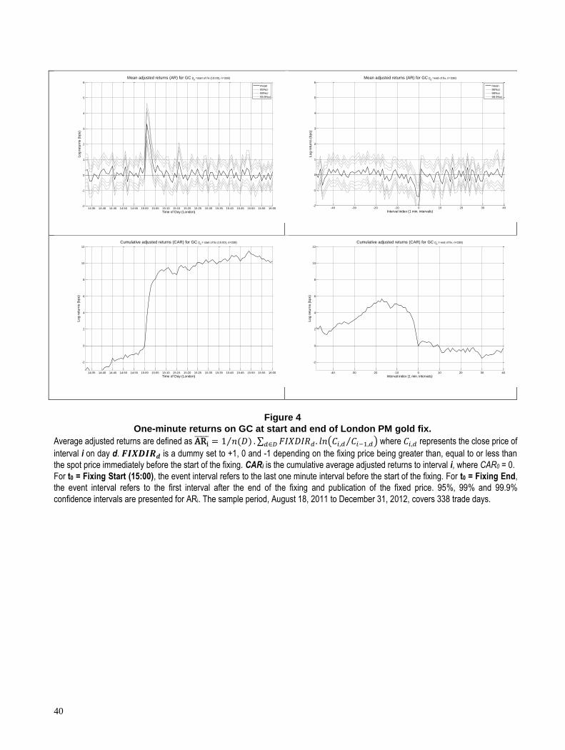
40

Figure 4

One-minute returns on GC at start and end of London PM gold fix.

Average adjusted returns are defined as ARi = 1 𝑛(𝐷)⁄ . ∑ 𝐹𝐼𝑋𝐷𝐼𝑅𝑑 . 𝑙𝑛(𝐶𝑖,𝑑 𝐶𝑖−1,𝑑⁄ )𝑑∈𝐷 where 𝐶𝑖,𝑑 represents the close price of

interval i on day d. 𝑭𝑰𝑿𝑫𝑰𝑹𝒅 is a dummy set to +1, 0 and -1 depending on the fixing price being greater than, equal to or less than

the spot price immediately before the start of the fixing. CARi is the cumulative average adjusted returns to interval i, where CAR0 = 0.

For t0 = Fixing Start (15:00), the event interval refers to the last one minute interval before the start of the fixing. For t0 = Fixing End,

the event interval refers to the first interval after the end of the fixing and publication of the fixed price. 95%, 99% and 99.9%

confidence intervals are presented for ARi. The sample period, August 18, 2011 to December 31, 2012, covers 338 trade days.

14:35 14:40 14:45 14:50 14:55 15:00 15:05 15:10 15:15 15:20 15:25 15:30 15:35 15:40 15:45 15:50 15:55 16:00-2

-1

0

1

2

3

4

5

6

Time of Day (London)

Lo

g r

etu

rns (

bp

s)

Mean adjusted returns (AR) for GC (t0 =start of fix (15:00), n=338)

mean

95%ci

99%ci

99.9%ci

-40 -30 -20 -10 0 10 20 30 40-2

-1

0

1

2

3

4

5

6

Mean adjusted returns (AR) for GC (t0 =end of fix, n=338)

Interval index (1 min. intervals)

Lo

g r

etu

rns (

bp

s)

mean

95%ci

99%ci

99.9%ci

14:35 14:40 14:45 14:50 14:55 15:00 15:05 15:10 15:15 15:20 15:25 15:30 15:35 15:40 15:45 15:50 15:55 16:00

-2

0

2

4

6

8

10

12

Time of Day (London)

Lo

g r

etu

rns (

bp

s)

Cumulative adjusted returns (CAR) for GC (t0 = start of fix (15:00), n=338)

-40 -30 -20 -10 0 10 20 30 40

-2

0

2

4

6

8

10

12

Cumulative adjusted returns (CAR) for GC (t0 = end of fix, n=338)

Interval index (1 min. intervals)

Lo

g r

etu

rns (

bp

s)

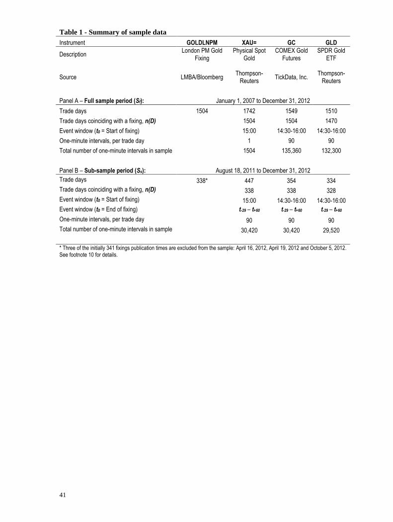
41

Table 1 - Summary of sample data

Instrument GOLDLNPM XAU= GC GLD

Description London PM Gold

Fixing Physical Spot

Gold COMEX Gold

Futures SPDR Gold

ETF

Source LMBA/Bloomberg Thompson-

Reuters TickData, Inc.

Thompson-Reuters

Panel A – Full sample period (Sf): January 1, 2007 to December 31, 2012

Trade days 1504 1742 1549 1510

Trade days coinciding with a fixing, n(D)

1504 1504 1470

Event window (t0 = Start of fixing) 15:00 14:30-16:00 14:30-16:00

One-minute intervals, per trade day 1 90 90

Total number of one-minute intervals in sample 1504 135,360 132,300

Panel B – Sub-sample period (Ss): August 18, 2011 to December 31, 2012

Trade days 338* 447 354 334

Trade days coinciding with a fixing, n(D)

338 338 328

Event window (t0 = Start of fixing) 15:00 14:30-16:00 14:30-16:00

Event window (t0 = End of fixing) t-29 – t+60 t-29 – t+60 t-29 – t+60

One-minute intervals, per trade day 90 90 90

Total number of one-minute intervals in sample 30,420 30,420 29,520

* Three of the initially 341 fixings publication times are excluded from the sample: April 16, 2012, April 19, 2012 and October 5, 2012. See footnote 10 for details.

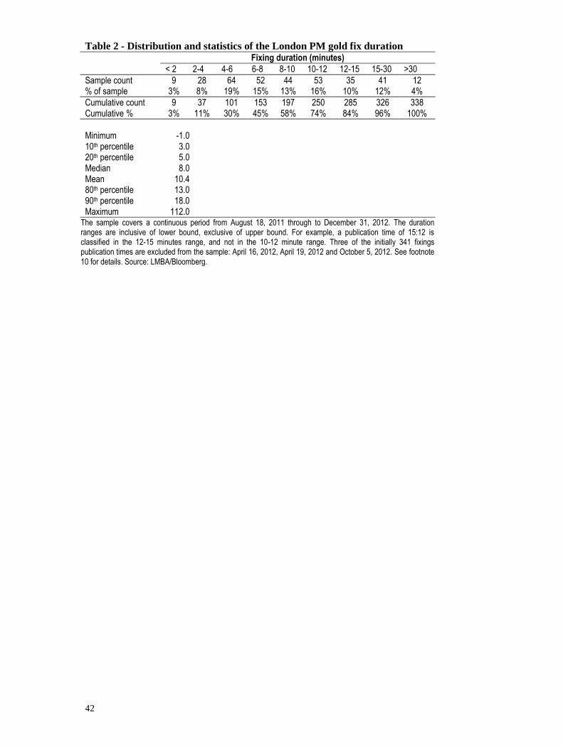
42

Table 2 - Distribution and statistics of the London PM gold fix duration Fixing duration (minutes)

< 2 2-4 4-6 6-8 8-10 10-12 12-15 15-30 >30

Sample count 9 28 64 52 44 53 35 41 12 % of sample 3% 8% 19% 15% 13% 16% 10% 12% 4%

Cumulative count 9 37 101 153 197 250 285 326 338 Cumulative % 3% 11% 30% 45% 58% 74% 84% 96% 100%

Minimum -1.0 10th percentile 3.0 20th percentile 5.0 Median 8.0 Mean 10.4 80th percentile 13.0 90th percentile 18.0 Maximum 112.0

The sample covers a continuous period from August 18, 2011 through to December 31, 2012. The duration ranges are inclusive of lower bound, exclusive of upper bound. For example, a publication time of 15:12 is classified in the 12-15 minutes range, and not in the 10-12 minute range. Three of the initially 341 fixings publication times are excluded from the sample: April 16, 2012, April 19, 2012 and October 5, 2012. See footnote 10 for details. Source: LMBA/Bloomberg.

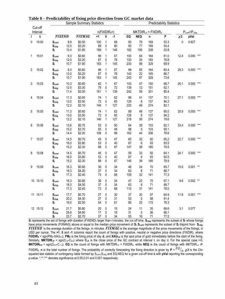
43

Table 8 – Predictability of fixing price direction from GC market data Sample Summary Statistics Predictability Statistics

Cut-off Interval

n(FIXDIRd=) MKTDIRi,d = FIXDIRd Pi,sml=Pi,big

i ti 𝑭𝑰𝑿𝑬𝑵𝑫 𝑭𝑰𝑿𝑴𝑨𝑮 +1 0 -1

EQ NEQ n

P

𝝌𝟐 pVal 0 15:00 Si,sml 8.8 $0.50

100 1 68

90 79 169

53.3

0 0.827

Si,big 12.0 $3.20

89 0 80

92 77 169

54.4 Si 10.4 $1.80

189 1 148

182 156 338

53.8

1 15:01 Si,sml 9.3 $0.60 96 1 67 100 64 164 61.0 12.4 0.000 ***

Si,big 12.0 $3.20

87 0 78

130 35 165

78.8 Si 10.7 $1.90

183 1 145

230 99 329

69.9

2 15:02 Si,sml 9.3 $0.60

96 1 67

99 65 164

60.4

29.3 0.000 ***

Si,big 12.0 $3.20

87 0 78

143 22 165

86.7 Si 10.7 $1.90

183 1 145

242 87 329

73.6

3 15:03 Si,sml 10.3 $0.60

82 1 67

103 47 150

68.7

26.1 0.000 ***

Si,big 12.5 $3.30

79 0 72

139 12 151

92.1 Si 11.4 $2.00

161 1 139

242 59 301

80.4

4 15:04 Si,sml 11.3 $0.60

74 1 62

96 41 137

70.1

27.1 0.000 ***

Si,big 13.0 $3.50

72 0 65

129 8 137

94.2 Si 12.2 $2.10

146 1 127

225 49 274

82.1

5 15:05 Si,sml 11.3 $0.60

74 1 62

89 48 137

65.0

35.9 0.000 ***

Si,big 13.0 $3.50

72 0 65

129 8 137

94.2 Si 12.2 $2.10

146 1 127

218 56 274

79.6

6 15:06 Si,sml 13.6 $0.70

53 0 50

64 39 103

62.1

33.4 0.000 ***

Si,big 15.2 $3.70

55 0 48

98 5 103

95.1 Si 14.4 $2.20

108 0 98

162 44 206

78.6

7 15:07 Si,sml 14.5 $0.70

45 0 47

60 32 92

65.2

22.7 0.000 ***

Si,big 16.0 $3.80

53 0 40

87 6 93

93.5 Si 15.2 $2.30

98 0 87

147 38 185

79.5

8 15:08 Si,sml 14.5 $0.70

45 0 47

59 33 92

64.1

24.1 0.000 ***

Si,big 16.0 $3.80

53 0 40

87 6 93

93.5 Si 15.2 $2.30

98 0 87

146 39 185

78.9

9 15:09 Si,sml 16.3 $0.80

36 0 34

46 24 70

65.7

10.6 0.001 **

Si,big 18.3 $4.00

37 0 34

63 8 71

88.7 Si 17.3 $2.40

73 0 68

109 32 141

77.3

10 15:10 Si,sml 16.3 $0.80

36 0 34

47 23 70

67.1

9.6 0.002 **

Si,big 18.3 $4.00

37 0 34

63 8 71

88.7 Si 17.3 $2.40

73 0 68

110 31 141

78.0

11 15:11 Si,sml 17.7 $0.70

27 0 30

37 20 57

64.9

11.8 0.001 ***

Si,big 20.2 $4.30

27 0 31

53 5 58

91.4 Si 19.0 $2.50

54 0 61

90 25 115

78.3

12 15:12 Si,sml 21.7 $0.80

20 0 15

24 11 35

68.6

3.1 0.077

Si,big 25.6 $4.60

17 0 19

31 5 36

86.1 Si 23.7 $2.70

37 0 34

55 16 71

77.5

Si represents the set of fixings with duration (FIXEND) larger than i minutes, the cut off time. Si,big represents the subset of Si whose fixings have price movements (FIXMAG) above or equal to the median price movement of Si. Si,sml represents the subset of Si disjoint from Si,big.

𝑭𝑰𝑿𝑬𝑵𝑫 is the average duration of the fixings, in minutes. 𝑭𝑰𝑿𝑴𝑨𝑮 is the average magnitude of the price movements of the fixings, in USD per ounce. The +1, 0 and -1 columns report the count of fixings with positive, neutral or negative price directions (FIXDIR), where FIXDIRd = sgn(PMd-XAU0,d), PMd is the fixing price of day d, and XAU0,d is the spot price of gold immediately before the start of the fixing. Similarly, MKTDIRi,d = sgn(Ci,d-C0,d) where Ci,d is the close price of the GC contract at interval i, on day d. For the special case i=0,

MKTDIR0,d = sgn(C0,d-C-1,d). EQ is the count of fixings with MKTDIRi,d = FIXDIRd, while NEQ is the count of fixings with MKTDIRi,d ≠

FIXDIRd. n is the total number of fixings. The probability of correctly forecasting the fixing direction is given by P = 𝐸𝑄

𝑛⁄ . 𝝌𝟐 is the Chi-

squared test statistic of contingency table formed by Si,sml,Si,big and EQ,NEQ for a given cut-off time ti with pVal reporting the corresponding

p-value. *,**,*** denotes significance at 0.05,0.01 and 0.001 respectively.

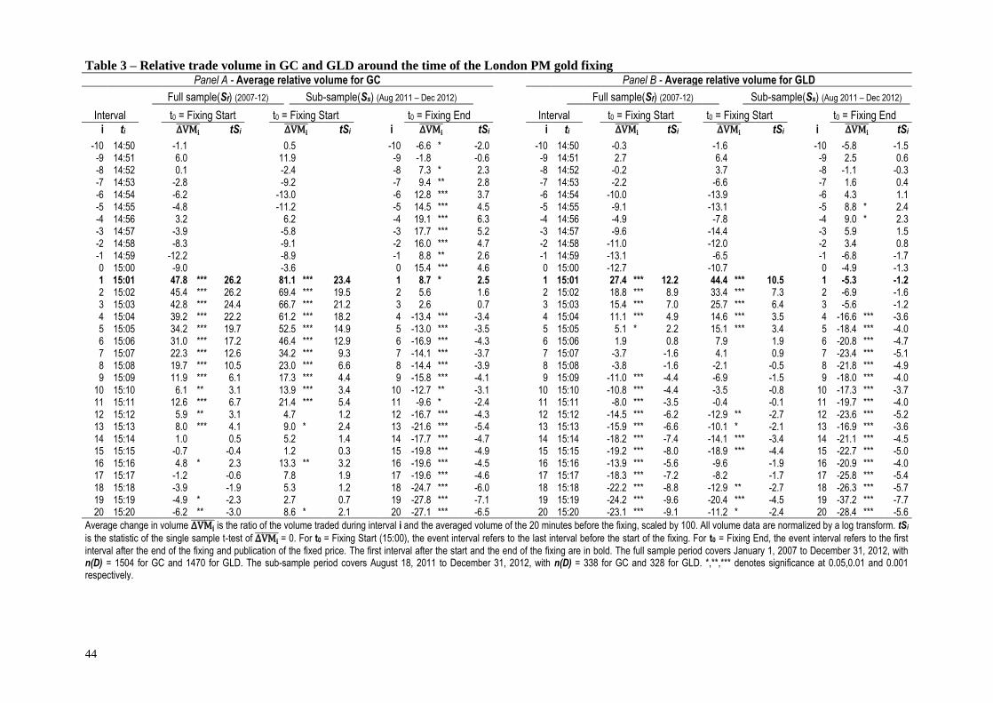
44

Table 3 – Relative trade volume in GC and GLD around the time of the London PM gold fixing Panel A - Average relative volume for GC Panel B - Average relative volume for GLD

Full sample(Sf) (2007-12) Sub-sample(Ss) (Aug 2011 – Dec 2012) Full sample(Sf) (2007-12) Sub-sample(Ss) (Aug 2011 – Dec 2012)

Interval t0 = Fixing Start t0 = Fixing Start t0 = Fixing End Interval t0 = Fixing Start t0 = Fixing Start t0 = Fixing End

i ti

∆VMi tSi

∆VMi tSi

i ∆VMi

tSi

i ti

∆VMi tSi

∆VMi tSi

i ∆VMi

tSi

-10 14:50

-1.1

0.5

-10 -6.6 * -2.0

-10 14:50

-0.3

-1.6

-10 -5.8

-1.5 -9 14:51

6.0

11.9

-9 -1.8

-0.6

-9 14:51

2.7

6.4

-9 2.5

0.6

-8 14:52

0.1

-2.4

-8 7.3 * 2.3

-8 14:52

-0.2

3.7

-8 -1.1

-0.3 -7 14:53

-2.8

-9.2

-7 9.4 ** 2.8

-7 14:53

-2.2

-6.6

-7 1.6

0.4

-6 14:54

-6.2

-13.0

-6 12.8 *** 3.7

-6 14:54

-10.0

-13.9

-6 4.3

1.1 -5 14:55

-4.8

-11.2

-5 14.5 *** 4.5

-5 14:55

-9.1

-13.1

-5 8.8 * 2.4

-4 14:56

3.2

6.2

-4 19.1 *** 6.3

-4 14:56

-4.9

-7.8

-4 9.0 * 2.3 -3 14:57

-3.9

-5.8

-3 17.7 *** 5.2

-3 14:57

-9.6

-14.4

-3 5.9

1.5

-2 14:58

-8.3

-9.1

-2 16.0 *** 4.7

-2 14:58

-11.0

-12.0

-2 3.4

0.8 -1 14:59

-12.2

-8.9

-1 8.8 ** 2.6

-1 14:59

-13.1

-6.5

-1 -6.8

-1.7

0 15:00

-9.0

-3.6

0 15.4 *** 4.6

0 15:00

-12.7

-10.7

0 -4.9

-1.3 1 15:01

47.8 *** 26.2

81.1 *** 23.4

1 8.7 * 2.5

1 15:01

27.4 *** 12.2

44.4 *** 10.5

1 -5.3

-1.2

2 15:02

45.4 *** 26.2

69.4 *** 19.5

2 5.6

1.6

2 15:02

18.8 *** 8.9

33.4 *** 7.3

2 -6.9

-1.6 3 15:03

42.8 *** 24.4

66.7 *** 21.2

3 2.6

0.7

3 15:03

15.4 *** 7.0

25.7 *** 6.4

3 -5.6

-1.2

4 15:04

39.2 *** 22.2

61.2 *** 18.2

4 -13.4 *** -3.4

4 15:04

11.1 *** 4.9

14.6 *** 3.5

4 -16.6 *** -3.6 5 15:05

34.2 *** 19.7

52.5 *** 14.9

5 -13.0 *** -3.5

5 15:05

5.1 * 2.2

15.1 *** 3.4

5 -18.4 *** -4.0

6 15:06

31.0 *** 17.2

46.4 *** 12.9

6 -16.9 *** -4.3

6 15:06

1.9

0.8

7.9

1.9

6 -20.8 *** -4.7 7 15:07

22.3 *** 12.6

34.2 *** 9.3

7 -14.1 *** -3.7

7 15:07

-3.7

-1.6

4.1

0.9

7 -23.4 *** -5.1

8 15:08

19.7 *** 10.5

23.0 *** 6.6

8 -14.4 *** -3.9

8 15:08

-3.8

-1.6

-2.1

-0.5

8 -21.8 *** -4.9 9 15:09

11.9 *** 6.1

17.3 *** 4.4

9 -15.8 *** -4.1

9 15:09

-11.0 *** -4.4

-6.9

-1.5

9 -18.0 *** -4.0

10 15:10

6.1 ** 3.1

13.9 *** 3.4

10 -12.7 ** -3.1

10 15:10

-10.8 *** -4.4

-3.5

-0.8

10 -17.3 *** -3.7 11 15:11

12.6 *** 6.7

21.4 *** 5.4

11 -9.6 * -2.4

11 15:11

-8.0 *** -3.5

-0.4

-0.1

11 -19.7 *** -4.0

12 15:12

5.9 ** 3.1

4.7

1.2

12 -16.7 *** -4.3

12 15:12

-14.5 *** -6.2

-12.9 ** -2.7

12 -23.6 *** -5.2 13 15:13

8.0 *** 4.1

9.0 * 2.4

13 -21.6 *** -5.4

13 15:13

-15.9 *** -6.6

-10.1 * -2.1

13 -16.9 *** -3.6

14 15:14

1.0

0.5

5.2

1.4

14 -17.7 *** -4.7

14 15:14

-18.2 *** -7.4

-14.1 *** -3.4

14 -21.1 *** -4.5 15 15:15

-0.7

-0.4

1.2

0.3

15 -19.8 *** -4.9

15 15:15

-19.2 *** -8.0

-18.9 *** -4.4

15 -22.7 *** -5.0

16 15:16

4.8 * 2.3

13.3 ** 3.2

16 -19.6 *** -4.5

16 15:16

-13.9 *** -5.6

-9.6

-1.9

16 -20.9 *** -4.0 17 15:17

-1.2

-0.6

7.8

1.9

17 -19.6 *** -4.6

17 15:17

-18.3 *** -7.2

-8.2

-1.7

17 -25.8 *** -5.4

18 15:18

-3.9

-1.9

5.3

1.2

18 -24.7 *** -6.0

18 15:18

-22.2 *** -8.8

-12.9 ** -2.7

18 -26.3 *** -5.7 19 15:19

-4.9 * -2.3

2.7

0.7

19 -27.8 *** -7.1

19 15:19

-24.2 *** -9.6

-20.4 *** -4.5

19 -37.2 *** -7.7

20 15:20

-6.2 ** -3.0

8.6 * 2.1

20 -27.1 *** -6.5

20 15:20

-23.1 *** -9.1

-11.2 * -2.4

20 -28.4 *** -5.6

Average change in volume ∆VMi is the ratio of the volume traded during interval i and the averaged volume of the 20 minutes before the fixing, scaled by 100. All volume data are normalized by a log transform. tSi

is the statistic of the single sample t-test of ∆VMi = 0. For t0 = Fixing Start (15:00), the event interval refers to the last interval before the start of the fixing. For t0 = Fixing End, the event interval refers to the first

interval after the end of the fixing and publication of the fixed price. The first interval after the start and the end of the fixing are in bold. The full sample period covers January 1, 2007 to December 31, 2012, with n(D) = 1504 for GC and 1470 for GLD. The sub-sample period covers August 18, 2011 to December 31, 2012, with n(D) = 338 for GC and 328 for GLD. *,**,*** denotes significance at 0.05,0.01 and 0.001 respectively.

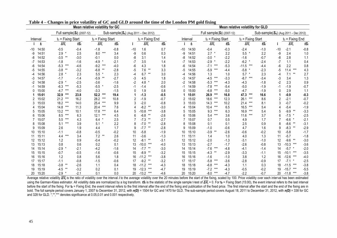
45

Table 4 – Changes in price volatility of GC and GLD around the time of the London PM gold fixing Mean relative volatility for GC Mean relative volatility for GLD

Full sample(Sf) (2007-12) Sub-sample(Ss) (Aug 2011 – Dec 2012) Full sample(Sf) (2007-12) Sub-sample(Ss) (Aug 2011 – Dec 2012)

Interval t0 = Fixing Start t0 = Fixing Start t0 = Fixing End Interval t0 = Fixing Start t0 = Fixing Start t0 = Fixing End

i ti

∆Vi tSi

∆Vi tSi

i ∆Vi

tSi

i ti

∆Vi tSi

∆Vi tSi

i ∆Vi

tSi

-10 14:50

-0.5

-0.4

-1.8

-0.8

-10 1.6

0.7

-10 14:50

-0.4

-0.3

-2.4

-1.0

-10 -2.1

-0.8 -9 14:51

2.9 * 2.5

8.0 *** 3.4

-9 0.6

0.3

-9 14:51

2.7 * 2.2

5.5 * 2.2

-9 2.4

1.0

-8 14:52

-3.5 ** -3.0

-0.1

0.0

-8 3.1

1.4

-8 14:52

-3.0 * -2.2

-1.6

-0.7

-8 2.8

1.1 -7 14:53

-1.8

-1.6

-4.9 * -2.1

-7 3.5

1.4

-7 14:53

-2.9 * -2.2

-6.2 * -2.4

-7 1.1

0.4

-6 14:54

-5.3 *** -4.6

-9.2 *** -4.0

-6 4.3

1.8

-6 14:54

-7.1 *** -5.3

-11.5 *** -4.4

-6 2.2

0.8 -5 14:55

-3.8 ** -3.2

-6.8 ** -2.8

-5 7.6 ** 3.3

-5 14:55

-5.9 *** -4.4

-5.8 * -2.3

-5 11.4 *** 4.3

-4 14:56

2.8 * 2.3

5.5 * 2.3

-4 6.7 ** 3.0

-4 14:56

1.3

1.0

5.7 * 2.3

-4 7.1 ** 2.7 -3 14:57

-1.7

-1.4

-5.9 ** -2.7

-3 4.5

1.8

-3 14:57

-4.5 *** -3.3

-8.7 *** -3.4

-3 3.4

1.3

-2 14:58

-2.9 * -2.5

-3.6

-1.6

-2 4.8 * 2.0

-2 14:58

-5.3 *** -4.3

-4.3

-1.8

-2 2.3

0.9 -1 14:59

-6.3 *** -5.3

-5.5 * -2.5

-1 -1.4

-0.6

-1 14:59

-7.8 *** -5.4

-5.0

-1.9

-1 -1.9

-0.7

0 15:00

-4.7 *** -4.0

-3.3

-1.5

0 1.9

0.8

0 15:00

-6.8 *** -5.0

-4.7

-1.9

0 2.9

1.1 1 15:01

32.9 *** 23.8

52.2 *** 19.4

1 -1.3

-0.5

1 15:01

26.9 *** 16.8

47.3 *** 16.6

1 -0.9

-0.3

2 15:02

21.2 *** 16.2

28.2 *** 10.8

2 -1.9

-0.7

2 15:02

18.6 *** 12.3

26.1 *** 8.6

2 -2.1

-0.7 3 15:03

18.2 *** 14.0

25.4 *** 9.9

3 -2.0

-0.8

3 15:03

14.3 *** 10.2

21.4 *** 8.1

3 -0.7

-0.2

4 15:04

14.8 *** 11.3

20.4 *** 7.6

4 -8.2 ** -3.0

4 15:04

10.4 *** 6.5

16.5 *** 5.4

4 -5.4

-1.9 5 15:05

13.2 *** 10.1

17.8 *** 6.4

5 -10.8 *** -3.8

5 15:05

9.3 *** 6.3

16.9 *** 5.4

5 -9.9 ** -3.3

6 15:06

8.5 *** 6.3

12.1 *** 4.5

6 -6.8 ** -2.6

6 15:06

5.4 *** 3.6

11.6 *** 3.7

6 -7.5 * -2.5 7 15:07

5.5 *** 4.3

6.4 * 2.5

7 -7.3 ** -2.7

7 15:07

0.7

0.5

4.9

1.7

7 -6.6 * -2.1

8 15:08

5.1 *** 3.9

5.1 * 2.2

8 -7.0 ** -2.8

8 15:08

0.1

0.1

2.5

0.9

8 -8.6 ** -3.1 9 15:09

2.6

1.9

4.4

1.7

9 -7.7 ** -2.8

9 15:09

-1.0

-0.6

4.7

1.6

9 -8.3 ** -2.9

10 15:10

-1.1

-0.8

-0.5

-0.2

10 -5.8

-1.9

10 15:10

-3.9 ** -2.6

-0.6

-0.2

10 -5.8

-1.7 11 15:11

4.4 *** 3.4

7.2 ** 2.6

11 -3.6

-1.3

11 15:11

1.4

1.0

4.0

1.3

11 -5.7

-1.8

12 15:12

1.2

0.9

-0.4

-0.2

12 -8.1 ** -3.1

12 15:12

-2.0

-1.3

-3.1

-1.0

12 -9.6 ** -3.0 13 15:13

0.8

0.6

0.2

0.1

13 -10.0 *** -4.0

13 15:13

-2.7

-1.7

-2.6

-0.8

13 -10.3 *** -3.6

14 15:14

-2.9 * -2.1

-4.2

-1.6

14 -7.7 ** -3.0

14 15:14

-7.6 *** -4.8

-4.1

-1.4

14 -5.7 * -2.0 15 15:15

-0.7

-0.5

-1.6

-0.6

15 -8.9 ** -3.2

15 15:15

-4.3 ** -2.9

-3.3

-1.1

15 -10.1 *** -3.5

16 15:16

1.2

0.8

5.6

1.8

16 -11.2 *** -3.8

16 15:16

-1.6

-1.0

3.8

1.2

16 -12.6 *** -4.0 17 15:17

-1.1

-0.8

-1.5

-0.6

17 -9.2 ** -3.2

17 15:17

-5.8 *** -3.6

-2.8

-0.9

17 -7.1 * -2.5

18 15:18

-3.8 ** -2.6

1.1

0.4

18 -11.2 *** -4.3

18 15:18

-6.8 *** -4.3

1.1

0.3

18 -11.5 *** -3.8 19 15:19

-4.5 ** -3.2

0.2

0.1

19 -12.3 *** -4.7

19 15:19

-7.2 *** -4.3

-0.5

-0.2

19 -15.7 *** -5.5

20 15:20

-2.9 * -2.1

0.1

0.0

20 -13.2 *** -4.6

20 15:20

-8.0 *** -4.7

-2.2

-0.7

20 -11.8 *** -3.8

Average relative volatility ∆Vi is the ratio of volatility over the interval i to the average volatility over the 20 minutes before the start of the fixing, scaled by 100. Price volatility over each interval has been estimated

using the Garman-Klass estimator. All volatility data are normalized by a log transform. tSi is the statistic of the single sample t-test of ∆Vi = 0. For t0 = Fixing Start (15:00), the event interval refers to the last interval

before the start of the fixing. For t0 = Fixing End, the event interval refers to the first interval after the end of the fixing and publication of the fixed price. The first interval after the start and the end of the fixing are in bold. The full sample period covers January 1, 2007 to December 31, 2012, with n(D) = 1504 for GC and 1470 for GLD. The sub-sample period covers August 18, 2011 to December 31, 2012, with n(D) = 338 for GC and 328 for GLD. *,**,*** denotes significance at 0.05,0.01 and 0.001 respectively.

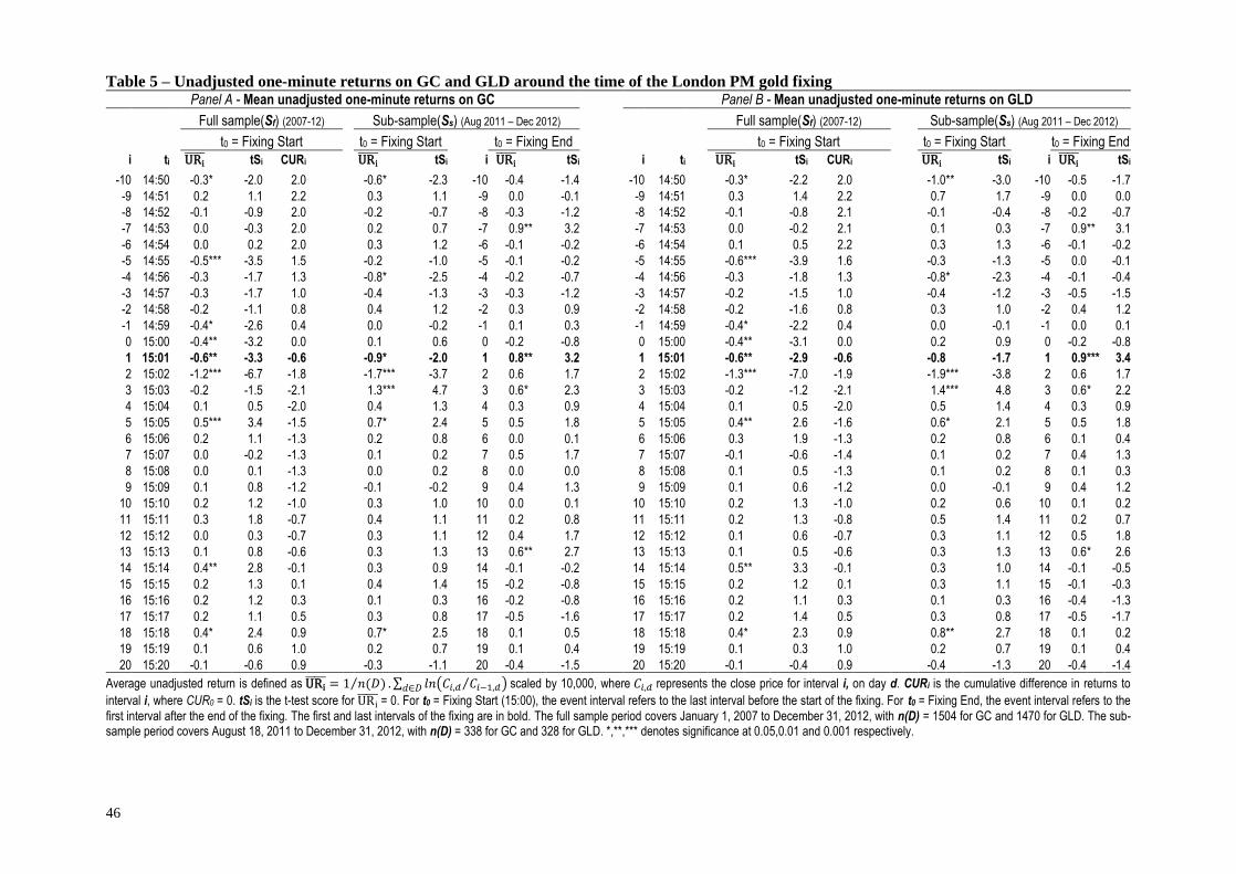
46

Table 5 – Unadjusted one-minute returns on GC and GLD around the time of the London PM gold fixing Panel A - Mean unadjusted one-minute returns on GC Panel B - Mean unadjusted one-minute returns on GLD

Full sample(Sf) (2007-12) Sub-sample(Ss) (Aug 2011 – Dec 2012) Full sample(Sf) (2007-12) Sub-sample(Ss) (Aug 2011 – Dec 2012) t0 = Fixing Start t0 = Fixing Start t0 = Fixing End t0 = Fixing Start t0 = Fixing Start t0 = Fixing End

i ti URi tSi CURi URi

tSi i URi tSi i ti URi

tSi CURi URi tSi i URi

tSi -10 14:50

-0.3 * -2.0 2.0

-0.6 * -2.3

-10 -0.4

-1.4

-10 14:50

-0.3 * -2.2 2.0

-1.0 ** -3.0

-10 -0.5

-1.7

-9 14:51

0.2

1.1 2.2

0.3

1.1

-9 0.0

-0.1

-9 14:51

0.3

1.4 2.2

0.7

1.7

-9 0.0

0.0

-8 14:52

-0.1

-0.9 2.0

-0.2

-0.7

-8 -0.3

-1.2

-8 14:52

-0.1

-0.8 2.1

-0.1

-0.4

-8 -0.2

-0.7

-7 14:53

0.0

-0.3 2.0

0.2

0.7

-7 0.9 ** 3.2

-7 14:53

0.0

-0.2 2.1

0.1

0.3

-7 0.9 ** 3.1

-6 14:54

0.0

0.2 2.0

0.3

1.2

-6 -0.1

-0.2

-6 14:54

0.1

0.5 2.2

0.3

1.3

-6 -0.1

-0.2

-5 14:55

-0.5 *** -3.5 1.5

-0.2

-1.0

-5 -0.1

-0.2

-5 14:55

-0.6 *** -3.9 1.6

-0.3

-1.3

-5 0.0

-0.1

-4 14:56

-0.3

-1.7 1.3

-0.8 * -2.5

-4 -0.2

-0.7

-4 14:56

-0.3

-1.8 1.3

-0.8 * -2.3

-4 -0.1

-0.4

-3 14:57

-0.3

-1.7 1.0

-0.4

-1.3

-3 -0.3

-1.2

-3 14:57

-0.2

-1.5 1.0

-0.4

-1.2

-3 -0.5

-1.5

-2 14:58

-0.2

-1.1 0.8

0.4

1.2

-2 0.3

0.9

-2 14:58

-0.2

-1.6 0.8

0.3

1.0

-2 0.4

1.2

-1 14:59

-0.4 * -2.6 0.4

0.0

-0.2

-1 0.1

0.3

-1 14:59

-0.4 * -2.2 0.4

0.0

-0.1

-1 0.0

0.1

0 15:00

-0.4 ** -3.2 0.0

0.1

0.6

0 -0.2

-0.8

0 15:00

-0.4 ** -3.1 0.0

0.2

0.9

0 -0.2

-0.8

1 15:01

-0.6 ** -3.3 -0.6

-0.9 * -2.0

1 0.8 ** 3.2

1 15:01

-0.6 ** -2.9 -0.6

-0.8

-1.7

1 0.9 *** 3.4

2 15:02

-1.2 *** -6.7 -1.8

-1.7 *** -3.7

2 0.6

1.7

2 15:02

-1.3 *** -7.0 -1.9

-1.9 *** -3.8

2 0.6

1.7

3 15:03

-0.2

-1.5 -2.1

1.3 *** 4.7

3 0.6 * 2.3

3 15:03

-0.2

-1.2 -2.1

1.4 *** 4.8

3 0.6 * 2.2

4 15:04

0.1

0.5 -2.0

0.4

1.3

4 0.3

0.9

4 15:04

0.1

0.5 -2.0

0.5

1.4

4 0.3

0.9

5 15:05

0.5 *** 3.4 -1.5

0.7 * 2.4

5 0.5

1.8

5 15:05

0.4 ** 2.6 -1.6

0.6 * 2.1

5 0.5

1.8

6 15:06

0.2

1.1 -1.3

0.2

0.8

6 0.0

0.1

6 15:06

0.3

1.9 -1.3

0.2

0.8

6 0.1

0.4

7 15:07

0.0

-0.2 -1.3

0.1

0.2

7 0.5

1.7

7 15:07

-0.1

-0.6 -1.4

0.1

0.2

7 0.4

1.3

8 15:08

0.0

0.1 -1.3

0.0

0.2

8 0.0

0.0

8 15:08

0.1

0.5 -1.3

0.1

0.2

8 0.1

0.3

9 15:09

0.1

0.8 -1.2

-0.1

-0.2

9 0.4

1.3

9 15:09

0.1

0.6 -1.2

0.0

-0.1

9 0.4

1.2

10 15:10

0.2

1.2 -1.0

0.3

1.0

10 0.0

0.1

10 15:10

0.2

1.3 -1.0

0.2

0.6

10 0.1

0.2

11 15:11

0.3

1.8 -0.7

0.4

1.1

11 0.2

0.8

11 15:11

0.2

1.3 -0.8

0.5

1.4

11 0.2

0.7

12 15:12

0.0

0.3 -0.7

0.3

1.1

12 0.4

1.7

12 15:12

0.1

0.6 -0.7

0.3

1.1

12 0.5

1.8

13 15:13

0.1

0.8 -0.6

0.3

1.3

13 0.6 ** 2.7

13 15:13

0.1

0.5 -0.6

0.3

1.3

13 0.6 * 2.6

14 15:14

0.4 ** 2.8 -0.1

0.3

0.9

14 -0.1

-0.2

14 15:14

0.5 ** 3.3 -0.1

0.3

1.0

14 -0.1

-0.5

15 15:15

0.2

1.3 0.1

0.4

1.4

15 -0.2

-0.8

15 15:15

0.2

1.2 0.1

0.3

1.1

15 -0.1

-0.3

16 15:16

0.2

1.2 0.3

0.1

0.3

16 -0.2

-0.8

16 15:16

0.2

1.1 0.3

0.1

0.3

16 -0.4

-1.3

17 15:17

0.2

1.1 0.5

0.3

0.8

17 -0.5

-1.6

17 15:17

0.2

1.4 0.5

0.3

0.8

17 -0.5

-1.7

18 15:18

0.4 * 2.4 0.9

0.7 * 2.5

18 0.1

0.5

18 15:18

0.4 * 2.3 0.9

0.8 ** 2.7

18 0.1

0.2

19 15:19

0.1

0.6 1.0

0.2

0.7

19 0.1

0.4

19 15:19

0.1

0.3 1.0

0.2

0.7

19 0.1

0.4

20 15:20

-0.1

-0.6 0.9

-0.3

-1.1

20 -0.4

-1.5

20 15:20

-0.1

-0.4 0.9

-0.4

-1.3

20 -0.4

-1.4

Average unadjusted return is defined as URi = 1 𝑛(𝐷)⁄ . ∑ 𝑙𝑛(𝐶𝑖,𝑑 𝐶𝑖−1,𝑑⁄ )𝑑∈𝐷 scaled by 10,000, where 𝐶𝑖,𝑑 represents the close price for interval i, on day d. CURi is the cumulative difference in returns to

interval i, where CUR0 = 0. tSi is the t-test score for URi = 0. For t0 = Fixing Start (15:00), the event interval refers to the last interval before the start of the fixing. For t0 = Fixing End, the event interval refers to the

first interval after the end of the fixing. The first and last intervals of the fixing are in bold. The full sample period covers January 1, 2007 to December 31, 2012, with n(D) = 1504 for GC and 1470 for GLD. The sub-sample period covers August 18, 2011 to December 31, 2012, with n(D) = 338 for GC and 328 for GLD. *,**,*** denotes significance at 0.05,0.01 and 0.001 respectively.

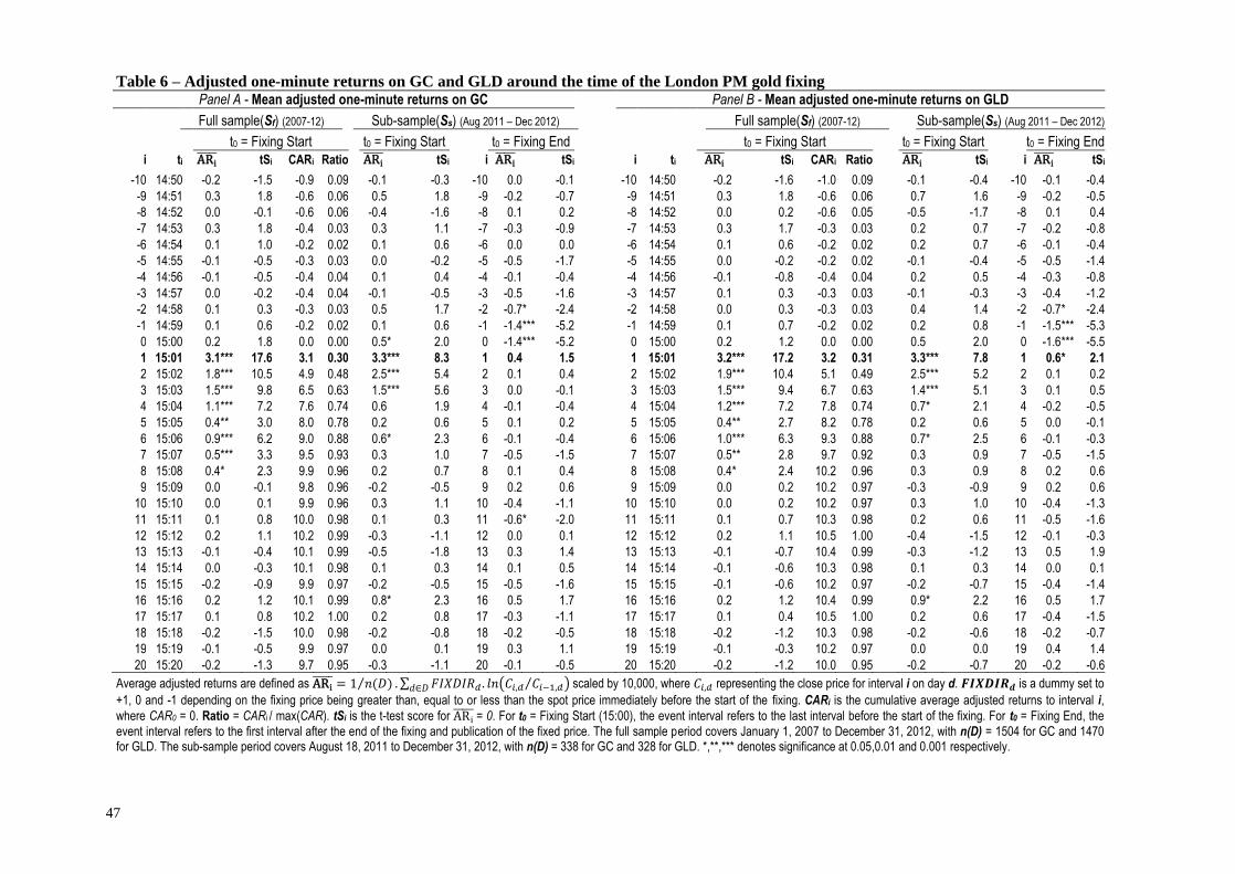
47

Table 6 – Adjusted one-minute returns on GC and GLD around the time of the London PM gold fixing Panel A - Mean adjusted one-minute returns on GC Panel B - Mean adjusted one-minute returns on GLD

Full sample(Sf) (2007-12) Sub-sample(Ss) (Aug 2011 – Dec 2012) Full sample(Sf) (2007-12) Sub-sample(Ss) (Aug 2011 – Dec 2012) t0 = Fixing Start t0 = Fixing Start t0 = Fixing End t0 = Fixing Start t0 = Fixing Start t0 = Fixing End

i ti ARi tSi CARi Ratio ARi

tSi i ARi tSi i ti ARi

tSi CARi Ratio ARi tSi i ARi

tSi -10 14:50

-0.2

-1.5 -0.9 0.09

-0.1

-0.3

-10 0.0

-0.1

-10 14:50

-0.2

-1.6 -1.0 0.09

-0.1

-0.4

-10 -0.1

-0.4

-9 14:51

0.3

1.8 -0.6 0.06

0.5

1.8

-9 -0.2

-0.7

-9 14:51

0.3

1.8 -0.6 0.06

0.7

1.6

-9 -0.2

-0.5

-8 14:52

0.0

-0.1 -0.6 0.06

-0.4

-1.6

-8 0.1

0.2

-8 14:52

0.0

0.2 -0.6 0.05

-0.5

-1.7

-8 0.1

0.4

-7 14:53

0.3

1.8 -0.4 0.03

0.3

1.1

-7 -0.3

-0.9

-7 14:53

0.3

1.7 -0.3 0.03

0.2

0.7

-7 -0.2

-0.8

-6 14:54

0.1

1.0 -0.2 0.02

0.1

0.6

-6 0.0

0.0

-6 14:54

0.1

0.6 -0.2 0.02

0.2

0.7

-6 -0.1

-0.4

-5 14:55

-0.1

-0.5 -0.3 0.03

0.0

-0.2

-5 -0.5

-1.7

-5 14:55

0.0

-0.2 -0.2 0.02

-0.1

-0.4

-5 -0.5

-1.4

-4 14:56

-0.1

-0.5 -0.4 0.04

0.1

0.4

-4 -0.1

-0.4

-4 14:56

-0.1

-0.8 -0.4 0.04

0.2

0.5

-4 -0.3

-0.8

-3 14:57

0.0

-0.2 -0.4 0.04

-0.1

-0.5

-3 -0.5

-1.6

-3 14:57

0.1

0.3 -0.3 0.03

-0.1

-0.3

-3 -0.4

-1.2

-2 14:58

0.1

0.3 -0.3 0.03

0.5

1.7

-2 -0.7 * -2.4

-2 14:58

0.0

0.3 -0.3 0.03

0.4

1.4

-2 -0.7 * -2.4

-1 14:59

0.1

0.6 -0.2 0.02

0.1

0.6

-1 -1.4 *** -5.2

-1 14:59

0.1

0.7 -0.2 0.02

0.2

0.8

-1 -1.5 *** -5.3

0 15:00

0.2

1.8 0.0 0.00

0.5 * 2.0

0 -1.4 *** -5.2

0 15:00

0.2

1.2 0.0 0.00

0.5

2.0

0 -1.6 *** -5.5

1 15:01

3.1 *** 17.6 3.1 0.30

3.3 *** 8.3

1 0.4

1.5

1 15:01

3.2 *** 17.2 3.2 0.31

3.3 *** 7.8

1 0.6 * 2.1

2 15:02

1.8 *** 10.5 4.9 0.48

2.5 *** 5.4

2 0.1

0.4

2 15:02

1.9 *** 10.4 5.1 0.49

2.5 *** 5.2

2 0.1

0.2

3 15:03

1.5 *** 9.8 6.5 0.63

1.5 *** 5.6

3 0.0

-0.1

3 15:03

1.5 *** 9.4 6.7 0.63

1.4 *** 5.1

3 0.1

0.5

4 15:04

1.1 *** 7.2 7.6 0.74

0.6

1.9

4 -0.1

-0.4

4 15:04

1.2 *** 7.2 7.8 0.74

0.7 * 2.1

4 -0.2

-0.5

5 15:05

0.4 ** 3.0 8.0 0.78

0.2

0.6

5 0.1

0.2

5 15:05

0.4 ** 2.7 8.2 0.78

0.2

0.6

5 0.0

-0.1

6 15:06

0.9 *** 6.2 9.0 0.88

0.6 * 2.3

6 -0.1

-0.4

6 15:06

1.0 *** 6.3 9.3 0.88

0.7 * 2.5

6 -0.1

-0.3

7 15:07

0.5 *** 3.3 9.5 0.93

0.3

1.0

7 -0.5

-1.5

7 15:07

0.5 ** 2.8 9.7 0.92

0.3

0.9

7 -0.5

-1.5

8 15:08

0.4 * 2.3 9.9 0.96

0.2

0.7

8 0.1

0.4

8 15:08

0.4 * 2.4 10.2 0.96

0.3

0.9

8 0.2

0.6

9 15:09

0.0

-0.1 9.8 0.96

-0.2

-0.5

9 0.2

0.6

9 15:09

0.0

0.2 10.2 0.97

-0.3

-0.9

9 0.2

0.6

10 15:10

0.0

0.1 9.9 0.96

0.3

1.1

10 -0.4

-1.1

10 15:10

0.0

0.2 10.2 0.97

0.3

1.0

10 -0.4

-1.3

11 15:11

0.1

0.8 10.0 0.98

0.1

0.3

11 -0.6 * -2.0

11 15:11

0.1

0.7 10.3 0.98

0.2

0.6

11 -0.5

-1.6

12 15:12

0.2

1.1 10.2 0.99

-0.3

-1.1

12 0.0

0.1

12 15:12

0.2

1.1 10.5 1.00

-0.4

-1.5

12 -0.1

-0.3

13 15:13

-0.1

-0.4 10.1 0.99

-0.5

-1.8

13 0.3

1.4

13 15:13

-0.1

-0.7 10.4 0.99

-0.3

-1.2

13 0.5

1.9

14 15:14

0.0

-0.3 10.1 0.98

0.1

0.3

14 0.1

0.5

14 15:14

-0.1

-0.6 10.3 0.98

0.1

0.3

14 0.0

0.1

15 15:15

-0.2

-0.9 9.9 0.97

-0.2

-0.5

15 -0.5

-1.6

15 15:15

-0.1

-0.6 10.2 0.97

-0.2

-0.7

15 -0.4

-1.4

16 15:16

0.2

1.2 10.1 0.99

0.8 * 2.3

16 0.5

1.7

16 15:16

0.2

1.2 10.4 0.99

0.9 * 2.2

16 0.5

1.7

17 15:17

0.1

0.8 10.2 1.00

0.2

0.8

17 -0.3

-1.1

17 15:17

0.1

0.4 10.5 1.00

0.2

0.6

17 -0.4

-1.5

18 15:18

-0.2

-1.5 10.0 0.98

-0.2

-0.8

18 -0.2

-0.5

18 15:18

-0.2

-1.2 10.3 0.98

-0.2

-0.6

18 -0.2

-0.7

19 15:19

-0.1

-0.5 9.9 0.97

0.0

0.1

19 0.3

1.1

19 15:19

-0.1

-0.3 10.2 0.97

0.0

0.0

19 0.4

1.4

20 15:20

-0.2

-1.3 9.7 0.95

-0.3

-1.1

20 -0.1

-0.5

20 15:20

-0.2

-1.2 10.0 0.95

-0.2

-0.7

20 -0.2

-0.6

Average adjusted returns are defined as ARi = 1 𝑛(𝐷)⁄ . ∑ 𝐹𝐼𝑋𝐷𝐼𝑅𝑑 . 𝑙𝑛(𝐶𝑖,𝑑 𝐶𝑖−1,𝑑⁄ )𝑑∈𝐷 scaled by 10,000, where 𝐶𝑖,𝑑 representing the close price for interval i on day d. 𝑭𝑰𝑿𝑫𝑰𝑹𝒅 is a dummy set to

+1, 0 and -1 depending on the fixing price being greater than, equal to or less than the spot price immediately before the start of the fixing. CARi is the cumulative average adjusted returns to interval i,

where CAR0 = 0. Ratio = CARi / max(CAR). tSi is the t-test score for ARi = 0. For t0 = Fixing Start (15:00), the event interval refers to the last interval before the start of the fixing. For t0 = Fixing End, the

event interval refers to the first interval after the end of the fixing and publication of the fixed price. The full sample period covers January 1, 2007 to December 31, 2012, with n(D) = 1504 for GC and 1470 for GLD. The sub-sample period covers August 18, 2011 to December 31, 2012, with n(D) = 338 for GC and 328 for GLD. *,**,*** denotes significance at 0.05,0.01 and 0.001 respectively.

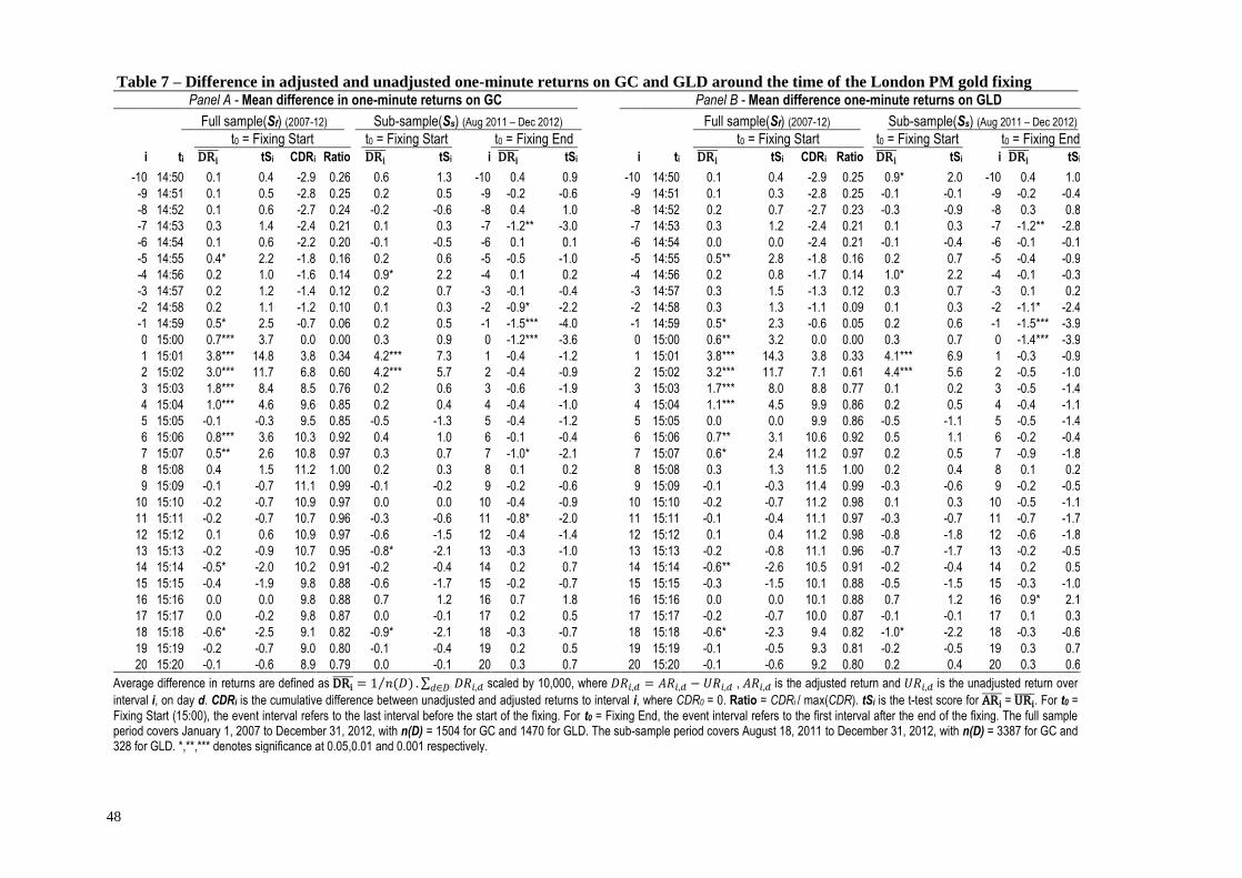
48

Table 7 – Difference in adjusted and unadjusted one-minute returns on GC and GLD around the time of the London PM gold fixing Panel A - Mean difference in one-minute returns on GC Panel B - Mean difference one-minute returns on GLD

Full sample(Sf) (2007-12) Sub-sample(Ss) (Aug 2011 – Dec 2012) Full sample(Sf) (2007-12) Sub-sample(Ss) (Aug 2011 – Dec 2012)

t0 = Fixing Start t0 = Fixing Start t0 = Fixing End t0 = Fixing Start t0 = Fixing Start t0 = Fixing End

i ti DRi tSi CDRi Ratio DRi

tSi i DRi tSi i ti DRi

tSi CDRi Ratio DRi tSi i DRi

tSi -10 14:50

0.1

0.4 -2.9 0.26

0.6

1.3

-10 0.4

0.9

-10 14:50

0.1

0.4 -2.9 0.25

0.9 * 2.0

-10 0.4

1.0

-9 14:51

0.1

0.5 -2.8 0.25

0.2

0.5

-9 -0.2

-0.6

-9 14:51

0.1

0.3 -2.8 0.25

-0.1

-0.1

-9 -0.2

-0.4

-8 14:52

0.1

0.6 -2.7 0.24

-0.2

-0.6

-8 0.4

1.0

-8 14:52

0.2

0.7 -2.7 0.23

-0.3

-0.9

-8 0.3

0.8

-7 14:53

0.3

1.4 -2.4 0.21

0.1

0.3

-7 -1.2 ** -3.0

-7 14:53

0.3

1.2 -2.4 0.21

0.1

0.3

-7 -1.2 ** -2.8

-6 14:54

0.1

0.6 -2.2 0.20

-0.1

-0.5

-6 0.1

0.1

-6 14:54

0.0

0.0 -2.4 0.21

-0.1

-0.4

-6 -0.1

-0.1

-5 14:55

0.4 * 2.2 -1.8 0.16

0.2

0.6

-5 -0.5

-1.0

-5 14:55

0.5 ** 2.8 -1.8 0.16

0.2

0.7

-5 -0.4

-0.9

-4 14:56

0.2

1.0 -1.6 0.14

0.9 * 2.2

-4 0.1

0.2

-4 14:56

0.2

0.8 -1.7 0.14

1.0 * 2.2

-4 -0.1

-0.3

-3 14:57

0.2

1.2 -1.4 0.12

0.2

0.7

-3 -0.1

-0.4

-3 14:57

0.3

1.5 -1.3 0.12

0.3

0.7

-3 0.1

0.2

-2 14:58

0.2

1.1 -1.2 0.10

0.1

0.3

-2 -0.9 * -2.2

-2 14:58

0.3

1.3 -1.1 0.09

0.1

0.3

-2 -1.1 * -2.4

-1 14:59

0.5 * 2.5 -0.7 0.06

0.2

0.5

-1 -1.5 *** -4.0

-1 14:59

0.5 * 2.3 -0.6 0.05

0.2

0.6

-1 -1.5 *** -3.9

0 15:00

0.7 *** 3.7 0.0 0.00

0.3

0.9

0 -1.2 *** -3.6

0 15:00

0.6 ** 3.2 0.0 0.00

0.3

0.7

0 -1.4 *** -3.9

1 15:01

3.8 *** 14.8 3.8 0.34

4.2 *** 7.3

1 -0.4

-1.2

1 15:01

3.8 *** 14.3 3.8 0.33

4.1 *** 6.9

1 -0.3

-0.9

2 15:02

3.0 *** 11.7 6.8 0.60

4.2 *** 5.7

2 -0.4

-0.9

2 15:02

3.2 *** 11.7 7.1 0.61

4.4 *** 5.6

2 -0.5

-1.0

3 15:03

1.8 *** 8.4 8.5 0.76

0.2

0.6

3 -0.6

-1.9

3 15:03

1.7 *** 8.0 8.8 0.77

0.1

0.2

3 -0.5

-1.4

4 15:04

1.0 *** 4.6 9.6 0.85

0.2

0.4

4 -0.4

-1.0

4 15:04

1.1 *** 4.5 9.9 0.86

0.2

0.5

4 -0.4

-1.1

5 15:05

-0.1

-0.3 9.5 0.85

-0.5

-1.3

5 -0.4

-1.2

5 15:05

0.0

0.0 9.9 0.86

-0.5

-1.1

5 -0.5

-1.4

6 15:06

0.8 *** 3.6 10.3 0.92

0.4

1.0

6 -0.1

-0.4

6 15:06

0.7 ** 3.1 10.6 0.92

0.5

1.1

6 -0.2

-0.4

7 15:07

0.5 ** 2.6 10.8 0.97

0.3

0.7

7 -1.0 * -2.1

7 15:07

0.6 * 2.4 11.2 0.97

0.2

0.5

7 -0.9

-1.8

8 15:08

0.4

1.5 11.2 1.00

0.2

0.3

8 0.1

0.2

8 15:08

0.3

1.3 11.5 1.00

0.2

0.4

8 0.1

0.2

9 15:09

-0.1

-0.7 11.1 0.99

-0.1

-0.2

9 -0.2

-0.6

9 15:09

-0.1

-0.3 11.4 0.99

-0.3

-0.6

9 -0.2

-0.5

10 15:10

-0.2

-0.7 10.9 0.97

0.0

0.0

10 -0.4

-0.9

10 15:10

-0.2

-0.7 11.2 0.98

0.1

0.3

10 -0.5

-1.1

11 15:11

-0.2

-0.7 10.7 0.96

-0.3

-0.6

11 -0.8 * -2.0

11 15:11

-0.1

-0.4 11.1 0.97

-0.3

-0.7

11 -0.7

-1.7

12 15:12

0.1

0.6 10.9 0.97

-0.6

-1.5

12 -0.4

-1.4

12 15:12

0.1

0.4 11.2 0.98

-0.8

-1.8

12 -0.6

-1.8

13 15:13

-0.2

-0.9 10.7 0.95

-0.8 * -2.1

13 -0.3

-1.0

13 15:13

-0.2

-0.8 11.1 0.96

-0.7

-1.7

13 -0.2

-0.5

14 15:14

-0.5 * -2.0 10.2 0.91

-0.2

-0.4

14 0.2

0.7

14 15:14

-0.6 ** -2.6 10.5 0.91

-0.2

-0.4

14 0.2

0.5

15 15:15

-0.4

-1.9 9.8 0.88

-0.6

-1.7

15 -0.2

-0.7

15 15:15

-0.3

-1.5 10.1 0.88

-0.5

-1.5

15 -0.3

-1.0

16 15:16

0.0

0.0 9.8 0.88

0.7

1.2

16 0.7

1.8

16 15:16

0.0

0.0 10.1 0.88

0.7

1.2

16 0.9 * 2.1

17 15:17

0.0

-0.2 9.8 0.87

0.0

-0.1

17 0.2

0.5

17 15:17

-0.2

-0.7 10.0 0.87

-0.1

-0.1

17 0.1

0.3

18 15:18

-0.6 * -2.5 9.1 0.82

-0.9 * -2.1

18 -0.3

-0.7

18 15:18

-0.6 * -2.3 9.4 0.82

-1.0 * -2.2

18 -0.3

-0.6

19 15:19

-0.2

-0.7 9.0 0.80

-0.1

-0.4

19 0.2

0.5

19 15:19

-0.1

-0.5 9.3 0.81

-0.2

-0.5

19 0.3

0.7

20 15:20

-0.1

-0.6 8.9 0.79

0.0

-0.1

20 0.3

0.7

20 15:20

-0.1

-0.6 9.2 0.80

0.2

0.4

20 0.3

0.6

Average difference in returns are defined as DRi = 1 𝑛(𝐷)⁄ . ∑ 𝐷𝑅𝑖,𝑑𝑑∈𝐷 scaled by 10,000, where 𝐷𝑅𝑖,𝑑 = 𝐴𝑅𝑖,𝑑 − 𝑈𝑅𝑖,𝑑 , 𝐴𝑅𝑖,𝑑 is the adjusted return and 𝑈𝑅𝑖,𝑑 is the unadjusted return over

interval i, on day d. CDRi is the cumulative difference between unadjusted and adjusted returns to interval i, where CDR0 = 0. Ratio = CDRi / max(CDR). tSi is the t-test score for ARi = URi

. For t0 =

Fixing Start (15:00), the event interval refers to the last interval before the start of the fixing. For t0 = Fixing End, the event interval refers to the first interval after the end of the fixing. The full sample period covers January 1, 2007 to December 31, 2012, with n(D) = 1504 for GC and 1470 for GLD. The sub-sample period covers August 18, 2011 to December 31, 2012, with n(D) = 3387 for GC and 328 for GLD. *,**,*** denotes significance at 0.05,0.01 and 0.001 respectively.