flexibility on switching option
DESCRIPTION
Flexibility on Switching OptionTRANSCRIPT

7/17/2019 Flexibility on Switching Option
http://slidepdf.com/reader/full/flexibility-on-switching-option 1/38
A Real Option Approach to Valuation of Manufacturing
Flexibility with 2 State Variables and Regime Switching
M.I.M. Wahab†, Chi-Guhn Lee†,1, Namkyu Park‡
†Department of Mechanical and Industrial Engineering
University of Toronto, Toronto, Ontario, M5S 3G8, Canada
‡Department of Industrial and Manufacturing Engineering
Wayne State University, Detroit, Michigan, 48202, USA
March 21, 2005
1Corresponding author can be reached at [email protected]

7/17/2019 Flexibility on Switching Option
http://slidepdf.com/reader/full/flexibility-on-switching-option 2/38
Abstract
We propose a real option approach to quantification of the value of flexibility in a manu-
facturing system, where the capacity level is optimally adjusted between two products so
as to maximize the total discounted expected profit over a given planning horizon. The
manufacturing system has three options in capacity adjustment: capacity expansion from
external sources, capacity contraction to external sources, and capacity switching within
the system. The demands for the two products are assumed to follow correlated Wiener
processes and to evolve through 2-stage product life: the growing regime first and then the
decaying regime. The original correlated processes are transformed into un-correlated ones
before a lattice is constructed, upon which a dynamic programming-based algorithm applied
to compute the value of manufacturing flexibility. Numerical studies on an example with
various combinations of cost parameters shed light on interesting aspects of manufacturing
flexibility.
Keywords: real option, regime switching, 2 state variables, product life cycle, lattice ap-
proach, manufacturing flexibility

7/17/2019 Flexibility on Switching Option
http://slidepdf.com/reader/full/flexibility-on-switching-option 3/38
1 INTRODUCTION
CBC News on October 29, 2004 excitingly reports Ford Motor’s grand investment plan on
its facilities in Oakville, Ontario as follows:
The company has decided to build a flexible manufacturing plant at the site.....
With the flexible manufacturing system, the Oakville plant will be capable of
producing up to four different vehicles based on two product platforms, Stevens,
Ford group vice president for Canada, Mexico, and South America, explained.
And the revamped operation will be able to rapidly respond to market fluctua-
tions, avoiding the time and expense required in traditional auto plant retooling.
Oakville will be Ford’s third flexible manufacturing facility. ..... By 2010, Ford
plans to have three-fourths of its 19 North American assembly plants converted
to the flexible system.
It is not only auto makers but firms in just about every industry sector who have suffered
from unsettled customer demands. The product life cycle has become shorter and shorter
and firms not being able to adapt to the whimsical market fail away. In an effort to remain
competitive in such a harsh business environment, more and more firms realize the impor-
tance of being flexible. For example, Ford Motor Co. plans to deliver 65 new Ford, Mercury
and Lincoln in five years and flexible manufacturing is rapidly recognized as a key cog in
unleashing new product to up market share.
While the importance of flexibility in manufacturing systems is well acknowledged, many
manufacturers fail to understand the benefits and the costs of being flexible. As a result it is
often seen too much flexible, not enough flexibility, or even wrong flexibility in manufacturing
1
7/17/2019 Flexibility on Switching Option
http://slidepdf.com/reader/full/flexibility-on-switching-option 4/38
systems. Such mismatches are almost always extremely costly since investments on flexible
manufacturing systems involve an astronomical dollar figures. In case of the Ford Motor’s
investment plan for the Oakville plant involves $1.2 billion dollars including $1 billion from
Ford Motor, $100 million from the Province of Ontario, and $100 million from the federal
government of Canada1.
In academia there have been continuous efforts to understand the value of manufacturing
flexibility for the last decade or so. A wide range of manufacturing options have been valued
using the financial theories mainly developed for the value of financial derivatives such as
options. Pindyck [17] and He and Pindyck [9] study capacity choice and expansion when
the system is irreversible. Tannous [19] develops a model to evaluate the effect of volume
flexibility and determines the optimal degree of automation. Triantis and Hodder [20] value
the option to switch the output mix over time in a flexible production system. Kulatilaka
[12] determines the value of flexibility of a system to produce specific output while switching
the production mode. Brennan and Schwartz [7] value interdependent options such as open,
close, reopen and abandon in natural resource investments. McDonald and Siegel [14] study
optimal timing of investment in an irreversible project, and McDonald and Siegel [15] study
investment project where there is an option to shut down. Majd and Pindyck [13] consider
the option to delay a irreversible project and determine the effect of time to build.
Despite the ample body of real options literature on manufacturing flexibility, it is often
the case that the nature of stochasticity of the underlying variable is assumed to be determin-
istic and constant. To address the shortcoming, Bollen [4] proposes a lattice framework with
regime switching, in which the probability distribution governing the uncertain evolution of
1All the dollar figures are in Canadian currency
2

7/17/2019 Flexibility on Switching Option
http://slidepdf.com/reader/full/flexibility-on-switching-option 5/38
underlying variable shifts across regimes. He then reports a significant error in valuing man-
ufacturing flexibility when such non-stationary behavior of the random variable is ignored.
His framework fits well in modeling the product life cycle, that usually starts in growing
phase, and then ends in decaying phase. However, his approach can only deal with a single
underlying variable, thereby fails to value the flexibility under which the manufacturing sys-
tem can reallocate its current capacity between different products within the system. This
flexibility is sometimes called the product-mix flexibility in the literature, which is one of the
most extensively studied flexibility type along with the volume flexibility. Manufacturing
flexibility types include product-mix flexibility, volume flexibility, new-product flexibility,
and delivery-time flexibility, routing flexibility, process flexibility, product flexibility, just to
name a few (more detailed discussion on various types of manufacturing flexibility can be
found in Bengtsson [2], Kulatilaka [12], Sethi and Sethi [18], among many).
We propose a lattice-based approach to valuation of manufacturing flexibility that has
three options: capacity expansion, capacity contraction, and capacity switching. Capacity
expansion and contraction constitute the volume flexibility, whereas capacity switching can
considered as product-mix flexibility. We assume that the demands for two products are
correlated and the correlation factor can change as the products shift toward the next phase
in their product life cycle. The manufacturing system can expand or contract its aggregate
capacity level through external sources as well as switching capacity dedicated to one product
to the other. The former flexibility will be called capacity expansion and capacity contraction,
while the latter will be called capacity switching in the paper.
This paper is organized as follows. Section 2.1 presents model that describes product
life cycles, demand process, cost and profit functions, fixed and flexible system. Section 3
3

7/17/2019 Flexibility on Switching Option
http://slidepdf.com/reader/full/flexibility-on-switching-option 6/38
describes lattice approach and flexibility valuation. Section 4 presents numerical example to
investigate the value of flexibility. Section 5 gives conclusions.
2 THE PROBLEM DEFINITION
In this section we define the market and the manufacturing system. The demand process
consists of two streams of random variables over time, whose stochastic characteristics may
change over time. We consider two manufacturing systems: one with fixed capacity and the
other with flexible capacity.
2.1 The Market Model
According to the literature of new product diffusion, demand for a new product typically
begins with start-up regime, and then growth regime. Later as the taste of the customer
changes or a new generation of product replaces existing product, the product life cycle
undergoes maturation regime, and finally decaying regime. Bass [1] proposes a forecasting
model based on two-regime product life cycle with exponential growth and exponential decay.
Bollen [4] addresses the value of manufacturing flexibility when the manufacturing system
produces a product with stochastic demand centered around two-regime product life cycle.
He points out that a significant error in the value of manufacturing flexibility is observed
when product life cycle is ignored.
Figure 1 depicts one possible realization of the future demand evolution of two products,
in which demands of both products grow up to time t1, and then demand of product 1 starts
decaying while that of product 2 continues to grow up to time t2(t2 > t1). After time t2,
4

7/17/2019 Flexibility on Switching Option
http://slidepdf.com/reader/full/flexibility-on-switching-option 7/38
demands of both products decay. We denote the combined regimes between time 0 and t1
as (G1, G2), the combined regime between time t1 and t2 as (D1, G2), and the other as
(D1, D2). When all possible realizations of the future demand evolution of both products
are considered, there will be one more combined regime (G1, D2). Thus, we have four
possible combinations of regimes when each of two products has two regimes. The number
of combinations becomes 9 when each product has 3 regimes, 16 when each has 4 regimes,
and so on.
Figure 1: Possible Combinations of Regimes
We consider a pair of correlated random demand processes, each of which has a two-regime
life cycle. Extension to more than two regimes can be done using a technique discussed in
Wahab and Lee [21]. Let θit denote demand of product i (i ∈ {A, B}) at time t. As commonly
assumed in real option literature, the continuously compounded rate of the demand of a
product within a regime is assumed to follow a stationary geometric Wiener process. The
5
7/17/2019 Flexibility on Switching Option
http://slidepdf.com/reader/full/flexibility-on-switching-option 8/38
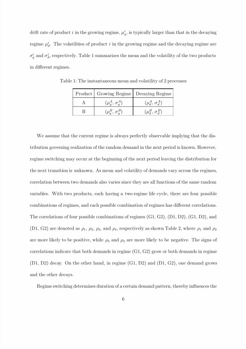
drift rate of product i in the growing regime, µig, is typically larger than that in the decaying
regime µid. The volatilities of product i in the growing regime and the decaying regime are
σig and σi
d, respectively. Table 1 summarizes the mean and the volatility of the two products
in different regimes.
Table 1: The instantaneous mean and volatility of 2 processes
Product Growing Regime Decaying Regime
A (µAg , σA
g ) (µAd , σA
d )
B (µBg , σB
g ) (µBd , σB
d )
We assume that the current regime is always perfectly observable implying that the dis-
tribution governing realization of the random demand in the next period is known. However,
regime switching may occur at the beginning of the next period leaving the distribution for
the next transition is unknown. As mean and volatility of demands vary across the regimes,
correlation between two demands also varies since they are all functions of the same random
variables. With two products, each having a two-regime life cycle, there are four possible
combinations of regimes, and each possible combination of regimes has different correlations.
The correlations of four possible combinations of regimes (G1, G2), (D1, D2), (G1, D2), and
(D1, G2) are denoted as ρ1, ρ2, ρ3, and ρ4, respectively as shown Table 2, where ρ1 and ρ2
are more likely to be positive, while ρ3 and ρ4 are more likely to be negative. The signs of
correlations indicate that both demands in regime (G1, G2) grow or both demands in regime
(D1, D2) decay. On the other hand, in regime (G1, D2) and (D1, G2), one demand grows
and the other decays.
Regime switching determines duration of a certain demand pattern, thereby influences the
6

7/17/2019 Flexibility on Switching Option
http://slidepdf.com/reader/full/flexibility-on-switching-option 9/38
Table 2: Correlation of between processes in each combination of regimes
Combinations of regimes (G1, G2) (D1, D2) (G1, D2) (D1, G2)
Correlation ρ1 ρ2 ρ3 ρ4
NPV of the manufacturing system. We employ the approach used in Bollen [4] by assuming
the probability of switching from the growing to the decaying regime in the next period is
cumulative normal distribution function in the time elapsed since the introduction of the
product to the market. This implies that pt, the probability of switching from the growing
to the decaying regime, conditional on still being in the growing regime, is as follows
pt =
t0
Φ(x|µs, σs)dx,
where Φ(s) is a normal distribution with a given mean µs and variance σs. Motivation behind
this approach is that there will be next-generation of product to replace an existing product
in the market after some years. The regime switching could also be modeled as function of
demand or cumulative demand using diffusion and substitution model by Norton and Bass
[16] or pure diffusion model by Bass [1].
We assume that regime switching is unidirectional; switching is always from the growing
to the decaying. Although this assumption is not necessary in our approach to valuation of
flexibility, it would make more sense in reality since products rarely revive its popularity once
it becomes insipid. Bidirectional regime switching makes sense in financial options pricing
and option pricing with multiple underlying assets that switch across multiple regime in a
bidirectional way can be found in Wahab and Lee [21].
7

7/17/2019 Flexibility on Switching Option
http://slidepdf.com/reader/full/flexibility-on-switching-option 10/38
2.2 The Manufacturing System
The cost model in this paper is motivated by a manufacturing firm who supplies dozens of
products in a wide range of price to a highly competitive market. The presence of many
competing firms supplying substituting products leaves the manufacturer with no room to
control the price. The price is set by the market so that the manufacturer is forced to be a
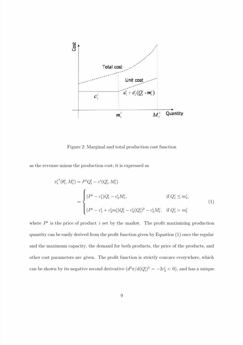
price taker and the cost function is as shown in Figure 2. In period t, the marginal production
cost, shown as a solid curve in Figure 2, is a constant ci1 while utilization is below a regular
capacity level mit, which is less than or equal to the maximum capacity level M it , and starts
increasing linearly with a slope ci2 as utilization exceeds the regular capacity. As a result the
total production cost, shown as a dotted curve, increases linearly up to the regular capacity
and quadratically above the regular capacity. There is also overhead cost ci3 to maintain a
unit capacity for product i(i ∈ {A, B}) in each period.
Let Qit be the production quantity of product i in period t. The cost function is expressed
as follows:
ci(Qit, M ii ) =
ci1Qit + ci3M it , if Qi
t ≤ mit,
ci1Qit + ci2(Qi
t − mit)Qi
t + ci3M it , if Qit > mi
t,
In order to determine the NPV of the system, profit from each product i must be calcu-
lated in each period t. The profit of product i in period t, denoted by πit(Qi
t, M ii ), is expressed
8
7/17/2019 Flexibility on Switching Option
http://slidepdf.com/reader/full/flexibility-on-switching-option 11/38
Figure 2: Marginal and total production cost function
as the revenue minus the production cost; it is expressed as
πit
∗
(θit, M it ) = P iQit − ci(Qit, M it )
=
(P i − ci1)Qit − ci3M it , if Qi
t ≤ mit,
(P i − ci1 + ci2mit)Qi
t − ci2(Qit)2 − ci3M it , if Qi
t > mit
(1)
where P i is the price of product i set by the market. The profit maximizing production
quantity can be easily derived from the profit function given by Equation (1) once the regular
and the maximum capacity, the demand for both products, the price of the products, and
other cost parameters are given. The profit function is strictly concave everywhere, which
can be shown by its negative second derivative (d2π/d(Qit)2 = −2ci2 < 0), and has a unique
9

7/17/2019 Flexibility on Switching Option
http://slidepdf.com/reader/full/flexibility-on-switching-option 12/38
minimum
Q̄it =
P i − ci1 + ci2mit
2ci2.
However, the production quantity exceeding the demand is clearly suboptimal, while it is
limited to the maximum capacity. Therefore, when demand θit, the maximum capacity M it
are given, the optimal production quantity of product i in period t is:
Qit
∗= min{θit,
Q̄it, M it}. (2)
Now that the profit in each period can be maximized by the production quantity given
in Equation (2), the next step is to maximize the total profit over a given planning horizon.
As mentioned earlier, the profit depends on the demand and the capacity. Assuming the
regular capacity is a certain fraction of the maximum capacity, the only control is the level
of the maximum capacity in each period since the demand is exogenous to the manufacturer.
In this paper we consider two systems: a fixed capacity system where the capacity ad-
justment is allowed only at the beginning of the project and a flexible capacity system where
the capacity adjustment is allowed throughout the life of the project. With a fixed capacity
system, the production quantities of product i in any period are bounded by optimal capacity
levels installed at time zero. Let π it
∗(θit, M i0) denote the optimal profit of product i in period
t when the maximum capacity is M i0 for product i. The net present value (NPV) of the fixed
system from time 1 to T is given by
NP V (M A0 , M B0 ) = −(cA4 M A0 + cB4 M B0 ) +T t=1
e−rt{E [πA∗t (θAt , M A0 )] + E [πB∗
t (θBt , M B0 )]}
where T is the terminal period of the project, r is the risk-free rate, and ci4 is the cost of
installing one unit of capacity for product i in period 0. An interesting point is how to set the
10

7/17/2019 Flexibility on Switching Option
http://slidepdf.com/reader/full/flexibility-on-switching-option 13/38
value of project life T , which can be viewed as the economic life of the manufacturing system.
This depends on various factors such as the demand for the products that the manufacturing
system is producing, the operating cost increasing over time due to aging, etc. The project
life T will have a huge impact on the project value and is uncertain for many reasons. One
of reasonable approaches is to define a probability distribution for project termination that
is a function of the duration of the project, cumulative demands, and so on. For simplicity
of exposition, we assume that T is given a priori. Extension to random termination would
not be a problem in our lattice-based approach.
Unlike the fixed capacity system, the flexible capacity system has the freedom to adjust
capacity. The initial capacity levels should be determined with consideration of the option
to adjust capacity and to respond optimally to the future demand evolution. In each period,
the flexible capacity system can not only expand and contract but also switch capacity from
one product to the other in an effort to maximize the total profit over a given horizon. We
assume that expansion, contraction and switching capacity take place between equally spaced
discrete capacity levels. This has been motivated by the fact that in industrial applications
the production capacity is determined by the number of machines or operators employed,
which is integer. Further, we assume that changes in the capacities are to be effective in
the following period to address time lag between decision made to change capacity and the
implementation of the capacity.
Capacity adjustment comes with cost or revenue. Let ∆ it be the change in the maximum
capacity level for product i between period t − 1 and t. That is,
∆it = M it − M it−1, i ∈ {A, B}.
11

7/17/2019 Flexibility on Switching Option
http://slidepdf.com/reader/full/flexibility-on-switching-option 14/38
A function S (∆At , ∆B
t ) is introduced to represent the cash flows in period t associated with
capacity adjustment decision made in period t − 1 to change the maximum capacity level for
product A by ∆At and that for product B by ∆B
t , effective in period t.
Cost parameters associated with capacity expansion and contraction are given in Table 3.
The flexible system, whenever it increases its maximum production level by a unit capacity
to produce product i (i ∈ {A, B}), incurs a fixed cost of si5 as well as a variable cost si1
fraction of the unit capacity installation cost ci4 for product i (i.e., si5 + si1ci4x where x is a
capacity increase). Similarly contraction of the maximum capacity for product i results in a
fixed cost si6 plus a variable cost equal to si2 fraction of the unit capacity installation cost ci4
for product i. Notice that the variable cost could be negative (i.e., positive revenue) in case
that the flexible system can find a good use for the capacity to be removed. Examples include
payment for producing OEM (original equipment manufacturer) products and salvage value
of machines to be removed.
Table 3: Cost parameters for capacity expansion and contraction
Capacity TypeExpansion Contraction
Variable Cost Fixed Cost Variable Cost Fixed Cost
Product A sA1 sA5 sA2 sA6
Product B sB1 sB5 sB2 sB6
Capacity switching between two products can be thought of as a combination of an ex-
pansion with one product and an contraction with the other. Since such capacity adjustment
takes place internally, cost or revenue associate with capacity switching may have to be based
on different parameters than those shown in Table 3. Parameters in Table 4 are for internal
12
7/17/2019 Flexibility on Switching Option
http://slidepdf.com/reader/full/flexibility-on-switching-option 15/38
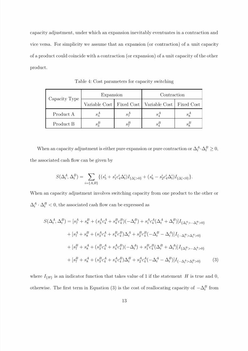
capacity adjustment, under which an expansion inevitably eventuates in a contraction and
vice versa. For simplicity we assume that an expansion (or contraction) of a unit capacity
of a product could coincide with a contraction (or expansion) of a unit capacity of the other
product.
Table 4: Cost parameters for capacity switching
Capacity TypeExpansion Contraction
Variable Cost Fixed Cost Variable Cost Fixed Cost
Product A sA3 sA7 sA4 sA8
Product B sB3 sB7 sB4 sB8
When an capacity adjustment is either pure expansion or pure contraction or ∆At ·∆B
t ≥ 0,
the associated cash flow can be given by
S (∆At , ∆B
t ) = i={A,B}
{(si5 + si1ci4∆it)I {∆i
t>0} + (si6 − si2ci4∆i
t)I {∆it<0}
}.
When an capacity adjustment involves switching capacity from one product to the other or
∆At · ∆B
t < 0, the associated cash flow can be expressed as
S (∆At , ∆B
t ) = [sA7 + sB8 + (sA3 cA4 + sB4 cB4 )(−∆Bt ) + sA1 cA4 (∆A
t + ∆Bt )]I {∆A
t >−∆Bt >0}
+ [sA7 + sB8 + (sA3 cA4 + sB4 cB4 )∆At + sB2 cB4 (−∆B
t − ∆At )]I {−∆B
t >∆At >0}
+ [sB7 + sA8 + (sB3 cA4 + sA4 cB4 )(−∆At ) + sB1 cB4 (∆Bt + ∆At )]I {∆Bt >−∆
At >0}
+ [sB7 + sA8 + (sB3 cA4 + sA4 cB4 )∆Bt + sA2 cA4 (−∆A
t − ∆Bt )]I {−∆A
t >∆Bt >0}
(3)
where I {H } is an indicator function that takes value of 1 if the statement H is true and 0,
otherwise. The first term in Equation (3) is the cost of reallocating capacity of −∆Bt from
13
7/17/2019 Flexibility on Switching Option
http://slidepdf.com/reader/full/flexibility-on-switching-option 16/38
product B to A and of expanding capacity of (∆At + ∆B
t ) for product A (recall ∆Bt < 0 and
∆At + ∆B
t is the pure capacity increase). The second term is for the case of reallocating
capacity of ∆A from product B to A and of further contracting capacity for product B by
(−∆Bt − ∆A
t ) (remember −∆Bt > 0 and |∆B
t | > |∆At |). The third and the fourth terms are
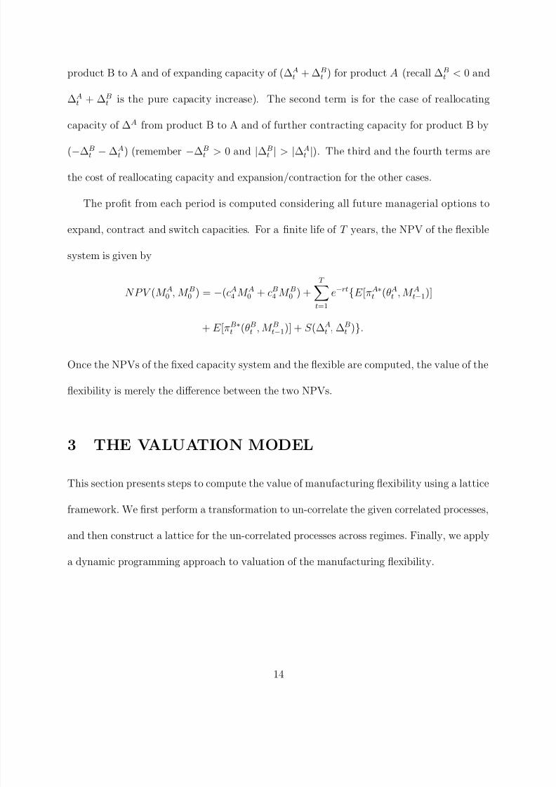
the cost of reallocating capacity and expansion/contraction for the other cases.
The profit from each period is computed considering all future managerial options to
expand, contract and switch capacities. For a finite life of T years, the NPV of the flexible
system is given by
NP V (M A0 , M B0 ) = −(cA4 M A0 + cB4 M B0 ) +T t=1
e−rt{E [πA∗t (θAt , M At−1)]
+ E [πB∗t (θBt , M Bt−1)] + S (∆A
t , ∆Bt )}.
Once the NPVs of the fixed capacity system and the flexible are computed, the value of the
flexibility is merely the difference between the two NPVs.
3 THE VALUATION MODEL
This section presents steps to compute the value of manufacturing flexibility using a lattice
framework. We first perform a transformation to un-correlate the given correlated processes,
and then construct a lattice for the un-correlated processes across regimes. Finally, we apply
a dynamic programming approach to valuation of the manufacturing flexibility.
14

7/17/2019 Flexibility on Switching Option
http://slidepdf.com/reader/full/flexibility-on-switching-option 17/38
3.1 Lattice Construction
Bollen [2] introduces pentanomial lattice for a single random process with two regimes. The
random process assumes a constant growth rate and a constant volatility within a regime.
His pentanomial lattice consists of a binomial lattice and a trinomial lattice: a binomial
lattice representing the growing regime and a trinomial lattice for the decaying regime. The
advantage of the pentanomial lattice is, although more nodes are branched out from a single
node, the reduced number of nodes in the whole lattice by setting up the step size of the
lattice so that nodes from different regimes merge into a single node.
In this paper we address the case of two random processes with regime switching. Re-
call that, in case of two random processes and two regimes for each process, we identified
four possible combinations of regimes in Section 2.1, where each combination consists of two
correlated processes with constant growth rates, volatilities, and a correlation factor. There-
fore, for each of four combinations of regimes, the lattice to be constructed and the original
continuous processes should have not only the first and the second moments but also the
joint moment to be matched. Although matching three moments or coefficients of moment
generating functions of two processes can be easily done as shown in Boyle [5, 6], matching
all three moments across the four combinations of regimes – not to mention the general case
of m variables with n j( j = 1, 2, . . . , m) regimes – is a big challenge. In this paper, we present
a technique to un-correlate two process in each of four pairs of correlated processes and to
build a single lattice for all the four combinations. Those who are interested in the general
case of m variables with n j( j = 1, 2, . . . , m) regimes can find a detailed exposition of the
general approach in Wahab and Lee [21]. It should be also noticed that the technique to be
15

7/17/2019 Flexibility on Switching Option
http://slidepdf.com/reader/full/flexibility-on-switching-option 18/38
presented in this paper may not be generalized to the case of m(m > 2) processes but can
be easily extended to the case with more than 2 regimes for each process.
Let x1 and x2 be two correlated processes as given below:
dx1 = α1dt + β 1dz 1, (4)
dx2 = α2dt + β 2dz 2, (5)
where αi and β i are constants, and dz 1 and dz 2 are correlated Wiener processes with corre-
lation factor ρ. Following Hull and White [11], a new pair of processes dy1 and dy2 can be
defined from the original correlated processes given in Equation (4) and (5).
dy1 = (α1β 2 + α2β 1)dt + β 1β 2
2(1 + ρ)dz 3,
dy2 = (α1β 2 − α2β 1)dt + β 1β 2
2(1 − ρ)dz 4,
where dz 3 and dz 4 are “un-correlated” Wiener processes. The new processes dy1 and dy2
have instantaneous mean of α1β 2 + α2β 1 and α1β 2 − α2β 1, respectively, and volatility of
β 1β 2
2(1 + ρ) and β 1β 2
2(1 − ρ), respectively.
Now consider a pair of correlated demand processes dθ1 and dθ2, which are in known
regimes. That is
dθ1 = µ1θ1dt + σ1θ1dz 1, (6)
dθ2 = µ2θ2dt + σ2θ2dz 2, (7)
where µi and σi are the growth rate and the volatility of process i in the known regimes,
and dz 1 and dz 2 are correlated Wiener processes. We convert, by using Ito’s Lemma [10],
the processes given in Equation (6) and (7) into the form of Equation (4) and (5) to obtain
16
7/17/2019 Flexibility on Switching Option
http://slidepdf.com/reader/full/flexibility-on-switching-option 19/38
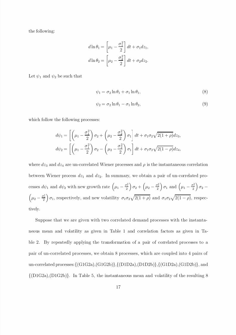
the following:
d ln θ1 =
µ1 − σ2
1
2
dt + σ1dz 1,
d ln θ2 =
µ2 − σ2
2
2
dt + σ2dz 2.
Let ψ1 and ψ2 be such that
ψ1 = σ2 ln θ1 + σ1 ln θ1, (8)
ψ2 = σ2 ln θ1 − σ1 ln θ2, (9)
which follow the following processes:
dψ1 =
µ1 − σ2
1
2
σ2 +
µ2 − σ2
2
2
σ1
dt + σ1σ2
2(1 + ρ)dz 3,
dψ2 =
µ1 − σ2
1
2
σ2 −
µ2 − σ2
2
2
σ1
dt + σ1σ2
2(1 − ρ)dz 4,
where dz 3 and dz 4 are un-correlated Wiener processes and ρ is the instantaneous correlation
between Wiener process dz 1 and dz 2. In summary, we obtain a pair of un-correlated pro-
cesses dψ1 and dψ2 with new growth rate
µ1 − σ212
σ2 +
µ2 − σ22
2
σ1 and
µ1 − σ21
2
σ2 −
µ2 − σ222
σ1, respectively, and new volatility σ1σ2
2(1 + ρ) and σ1σ2
2(1 − ρ), respec-
tively.
Suppose that we are given with two correlated demand processes with the instanta-
neous mean and volatility as given in Table 1 and correlation factors as given in Ta-
ble 2. By repeatedly applying the transformation of a pair of correlated processes to a
pair of un-correlated processes, we obtain 8 processes, which are coupled into 4 pairs of
un-correlated processes:{(G1G2a),(G1G2b)},{(D1D2a),(D1D2b)},{(G1D2a),(G1D2b)}, and
{(D1G2a),(D1G2b)}. In Table 5, the instantaneous mean and volatility of the resulting 8
17

7/17/2019 Flexibility on Switching Option
http://slidepdf.com/reader/full/flexibility-on-switching-option 20/38
Table 5: Instantaneous mean and volatility of 8 un-correlated processes
Process Instantaneous Mean Instantaneous Volatility
G1G2a µ1 = (µA
g − (σAg )
2
2 )σB
g
+ (µB
g − (σBg )
2
2 )σA
g
σ1 = σA
g
σB
g 2(1 + ρ1)
G1G2b µ2 = (µAg − (σAg )
2
2 )σBg − (µB
g − (σBg )2
2 )σAg σ2 = σA
g σBg
2(1 − ρ1)
D1D2a µ3 = (µAd − (σAd )
2
2 )σBd + (µB
d − (σBd )2
2 )σAd σ3 = σA
d σBd
2(1 + ρ2)
D1D2b µ4 = (µAd − (σAd )
2
2 )σB
d − (µBd − (σBd )
2
2 )σA
d σ4 = σAd σB
d
2(1 − ρ2)
G1D2a µ5 = (µAg − (σAg )
2
2 )σB
d + (µBd − (σB
d )2
2 )σA
g σ5 = σAg σB
d
2(1 + ρ3)
G1D2b µ6 = (µAg − (σAg )
2
2 )σB
d − (µBd − (σBd )
2
2 )σA
g σ6 = σAg σB
d
2(1 − ρ3)
D1G2a µ7 = (µAd
−
(σAd )2
2 )σB
g + (µBg
−
(σBg )2
2 )σA
d σ7 = σAd σB
g 2(1 + ρ4)
D1G2b µ8 = (µAd − (σAd )
2
2 )σBg − (µB
g − (σBg )2
2 )σAd σ8 = σA
d σBg
2(1 − ρ4)
processes are shown, where process G1G2a and G1G2b are from the original demand process
of product A in the growing regime G1 and that of product B in the growing regime G2,
process D1D2a and D1D2b are from the two original correlated processes in their decaying
regime, process G1D2a and G1D2b from original process for product A in the growing and
B in the decaying, and process D1G2a and D1G2b from original process A in decaying and
B in growing regime. Therefore, process G1G2a, D1D2a, G1D2a, and D1G2a can be seen as
four regimes of one un-correlated process and processes G1G2b, D1D2b, G1D2b, and D1G2b
as four regimes of the other new un-correlated process.
The next step is to build a lattice for the un-correlated processes, each of which has four
regimes with known means and known volatilities. In what follows, the exposition assumes
the general case of a single process with n regimes. As discussed in Bollen [3] and Wahab
and Lee [21], the step size of the lattice of all regimes except for one must be adjusted so that
further branching results in nodes to be merged into a fewer number of nodes. The step size
18

7/17/2019 Flexibility on Switching Option
http://slidepdf.com/reader/full/flexibility-on-switching-option 21/38
of n − 1 regimes must be adjusted so that all the nodes generated for n regimes are evenly
spaced. In order to determine the n − 1 regimes of which step sizes are to be adjusted, step
size of all n regimes are independently calculated as follows:
σ2i h + µ2
ih2, i = 1, 2, . . . , n ,
where µi and σi are mean and volatility in regime i, and h is the time interval corresponding
to a layer of the lattice. More details of the standard binomial tree construction can be found
in Cox et al. [8], Hull [10], among many. Let φ1, φ2, ....,φn be step size of regime 1, 2, . . . , n,
respectively (i.e., φi =
σ2i h + µ
2ih
2
for i = 1, 2, . . . , n). After re-naming the regimes so that
φ1 < φ2 < φ3,..,< φn, we set φ = max(φ1, φ22
, φ33
, ....., φnn
). Let φ = φkk
(i.e.,φkk ≥ φj
j , ∀ j),
then the step size φ j should be as follows:
φ j =
φk, if j = k,
j φkk
, if j = k.
(10)
Notice that the step size is adjusted so as to ensure that nodes are spaced equidistant from
each other.
The regime with step size φk must be constructed by a binomial lattice and the other
regimes (∀ j = 1, 2, 3,..,n, and j = k) must be constructed by trinomial lattices. The
conditional probabilities for all the branches emanating from a node can be computed by
matching the first and the second moments of the lattice and the given continuous processes.
The conditional branch probability of binomial lattice for regime k is given by
πφk,u = 1
2
1 +
µkh
φk
, (11)
πφk,d = 1 − πφk,u, (12)
19
7/17/2019 Flexibility on Switching Option
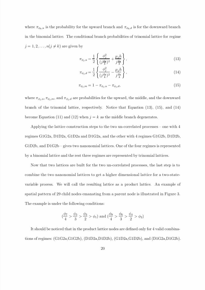
http://slidepdf.com/reader/full/flexibility-on-switching-option 22/38
where πφk,u is the probability for the upward branch and πφk,d is for the downward branch
in the binomial lattice. The conditional branch probabilities of trinomial lattice for regime
j = 1, 2, . . . , n( j
= k) are given by
πφj ,u = 1
2
φ2
j
( j φkk
)2+
µ jh
j φkk
, (13)
πφj ,d = 1
2
φ2
j
( j φkk
)2− µ jh
j φkk
, (14)
πφj ,m = 1 − πφj ,u − πφj,d, (15)
where πφj ,u, πφj ,m, and πφj ,d are probabilities for the upward, the middle, and the downward
branch of the trinomial lattice, respectively. Notice that Equation (13), (15), and (14)
become Equation (11) and (12) when j = k as the middle branch degenerates.
Applying the lattice construction steps to the two un-correlated processes – one with 4
regimes G1G2a, D1D2a, G1D2a and D1G2a, and the other with 4 regimes G1G2b, D1D2b,
G1D2b, and D1G2b – gives two nanonomial lattices. One of the four regimes is represented
by a binomial lattice and the rest three regimes are represented by trinomial lattices.
Now that two lattices are built for the two un-correlated processes, the last step is to
combine the two nanonomial lattices to get a higher dimensional lattice for a two-state-
variable process. We will call the resulting lattice as a product lattice. An example of
spatial pattern of 29 child nodes emanating from a parent node is illustrated in Figure 3.
The example is under the following conditions:
(φ7
4 >
φ5
3 >
φ3
2 > φ1) and (
φ8
4 >
φ6
3 >
φ4
2 > φ2)
It should be noticed that in the product lattice nodes are defined only for 4 valid combina-
tions of regimes: (G1G2a,G1G2b), (D1D2a,D1D2b), (G1D2a,G1D2b), and (D1G2a,D1G2b).
20

7/17/2019 Flexibility on Switching Option
http://slidepdf.com/reader/full/flexibility-on-switching-option 23/38
For example, nodes are generated for a combination (G1G2a, G1G2b) but not for a com-
bination (G1G2a, D1D2b). Therefore, each parent node has 29 child nodes, with 3 nodes
stacked at the center node, rather than 81. Conditional branch probability of each branch
of the product lattice is computed as the product of two conditional branch probabilities of
the two corresponding branches from the original nanonomial lattice.
Figure 3: Pattern of Child Nodes
Numbers in the parenthesis at each node of the lattice in Figure 3 are conditional probabil-
ities from the two nanonomial lattices. These probabilities can be calculated using Equation
(11) through (14). First subscript of the probability indicates the step size of the branch that
21
7/17/2019 Flexibility on Switching Option
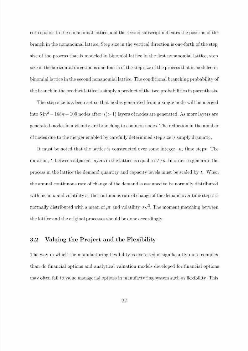
http://slidepdf.com/reader/full/flexibility-on-switching-option 24/38
corresponds to the nonanomial lattice, and the second subscript indicates the position of the
branch in the nonanoimal lattice. Step size in the vertical direction is one-forth of the step
size of the process that is modeled in binomial lattice in the first nonanomial lattice; step
size in the horizontal direction is one-fourth of the step size of the process that is modeled in
binomial lattice in the second nonanomial lattice. The conditional branching probability of
the branch in the product lattice is simply a product of the two probabilities in parenthesis.
The step size has been set so that nodes generated from a single node will be merged
into 64n2 − 168n + 109 nodes after n(> 1) layers of nodes are generated. As more layers are
generated, nodes in a vicinity are branching to common nodes. The reduction in the number
of nodes due to the merger enabled by carefully determined step size is simply dramatic.
It must be noted that the lattice is constructed over some integer, n, time steps. The
duration, t, between adjacent layers in the lattice is equal to T /n. In order to generate the
process in the lattice the demand quantity and capacity levels must be scaled by t. When
the annual continuous rate of change of the demand is assumed to be normally distributed
with mean µ and volatility σ, the continuous rate of change of the demand over time step t is
normally distributed with a mean of µt and volatility σ√
t. The moment matching between
the lattice and the original processes should be done accordingly.
3.2 Valuing the Project and the Flexibility
The way in which the manufacturing flexibility is exercised is significantly more complex
than do financial options and analytical valuation models developed for financial options
may often fail to value managerial options in manufacturing system such as flexibility. This
22
7/17/2019 Flexibility on Switching Option
http://slidepdf.com/reader/full/flexibility-on-switching-option 25/38
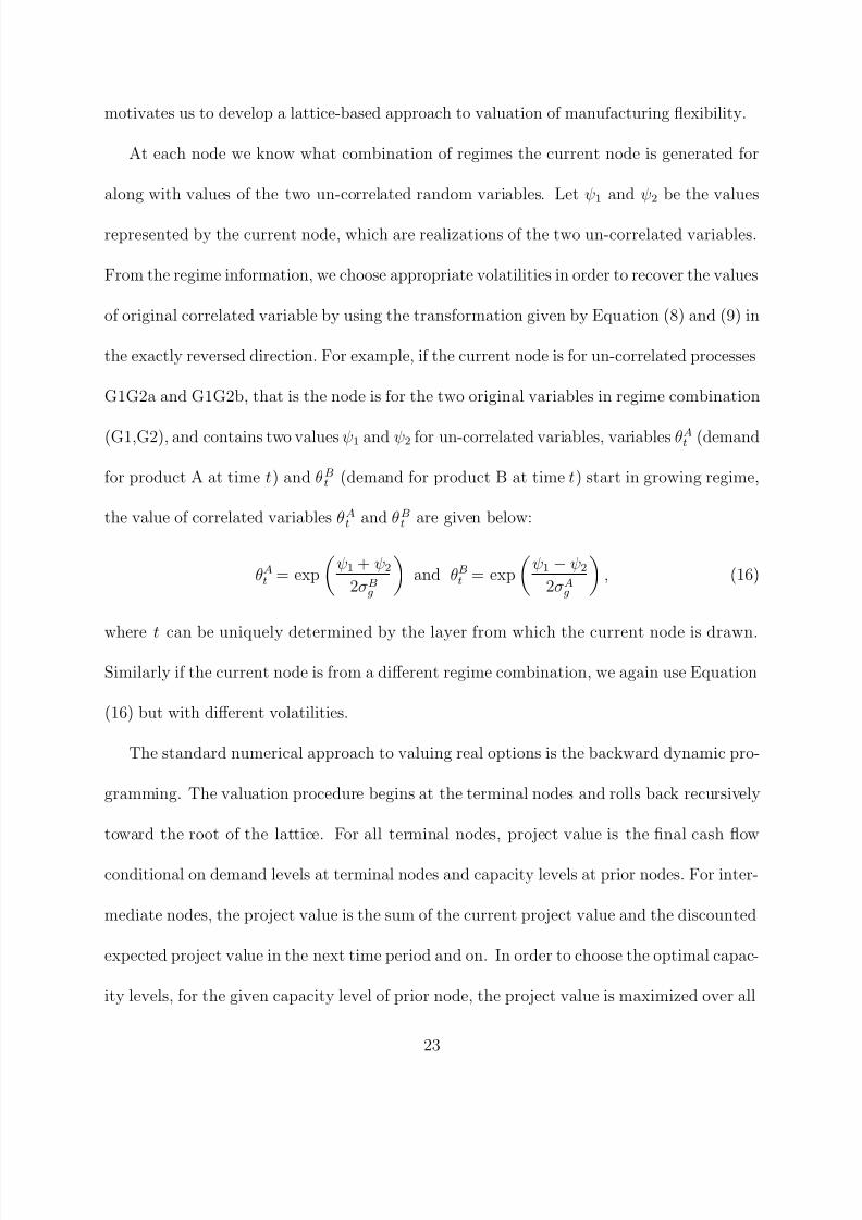
motivates us to develop a lattice-based approach to valuation of manufacturing flexibility.
At each node we know what combination of regimes the current node is generated for
along with values of the two un-correlated random variables. Let ψ1 and ψ2 be the values
represented by the current node, which are realizations of the two un-correlated variables.
From the regime information, we choose appropriate volatilities in order to recover the values
of original correlated variable by using the transformation given by Equation (8) and (9) in
the exactly reversed direction. For example, if the current node is for un-correlated processes
G1G2a and G1G2b, that is the node is for the two original variables in regime combination
(G1,G2), and contains two values ψ1 and ψ2 for un-correlated variables, variables θAt (demand
for product A at time t) and θBt (demand for product B at time t) start in growing regime,
the value of correlated variables θAt and θBt are given below:
θAt = exp
ψ1 + ψ2
2σBg
and θBt = exp
ψ1 − ψ2
2σAg
, (16)
where t can be uniquely determined by the layer from which the current node is drawn.
Similarly if the current node is from a different regime combination, we again use Equation
(16) but with different volatilities.
The standard numerical approach to valuing real options is the backward dynamic pro-
gramming. The valuation procedure begins at the terminal nodes and rolls back recursively
toward the root of the lattice. For all terminal nodes, project value is the final cash flow
conditional on demand levels at terminal nodes and capacity levels at prior nodes. For inter-
mediate nodes, the project value is the sum of the current project value and the discounted
expected project value in the next time period and on. In order to choose the optimal capac-
ity levels, for the given capacity level of prior node, the project value is maximized over all
23
7/17/2019 Flexibility on Switching Option
http://slidepdf.com/reader/full/flexibility-on-switching-option 26/38
possible capacity levels. Therefore, the discounted expected future values reflect the possibil-
ity of capacity adjustment (expansion, contraction and switching). The expectation is also
with respect to possible regime switching in the next period. The value of the project (or
the manufacturing system over a given horizon) is simply the discounted expected project
value at the root node of the lattice. The same calculation with fixed capacity levels for
two product gives the project value of the fixed manufacturing system. The value of the
flexibility is merely the difference between the two project values.
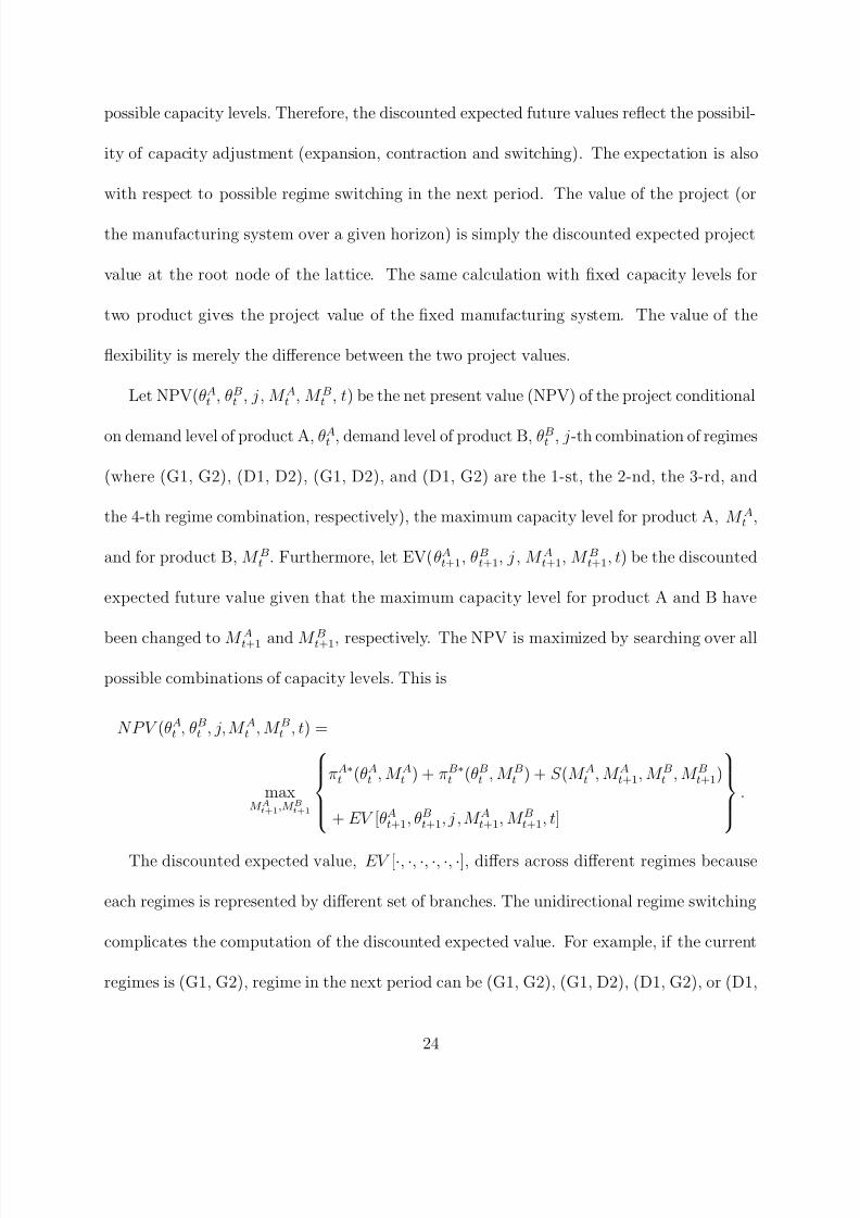
Let NPV(θAt , θBt , j, M At , M Bt , t) be the net present value (NPV) of the project conditional
on demand level of product A, θAt , demand level of product B, θBt , j-th combination of regimes
(where (G1, G2), (D1, D2), (G1, D2), and (D1, G2) are the 1-st, the 2-nd, the 3-rd, and
the 4-th regime combination, respectively), the maximum capacity level for product A, M At ,
and for product B, M Bt . Furthermore, let EV(θAt+1, θBt+1, j , M At+1, M Bt+1, t) be the discounted
expected future value given that the maximum capacity level for product A and B have
been changed to M At+1 and M
Bt+1, respectively. The NPV is maximized by searching over all
possible combinations of capacity levels. This is
NP V (θAt , θBt , j, M At , M Bt , t) =
maxM At+1,M Bt+1
πA∗t (θAt , M At ) + πB∗
t (θBt , M Bt ) + S (M At , M At+1, M Bt , M Bt+1)
+ EV [θAt+1, θBt+1, j , M At+1, M Bt+1, t]
.
The discounted expected value, EV [·, ·, ·, ·, ·, ·], differs across different regimes because
each regimes is represented by different set of branches. The unidirectional regime switching
complicates the computation of the discounted expected value. For example, if the current
regimes is (G1, G2), regime in the next period can be (G1, G2), (G1, D2), (D1, G2), or (D1,
24
7/17/2019 Flexibility on Switching Option
http://slidepdf.com/reader/full/flexibility-on-switching-option 27/38
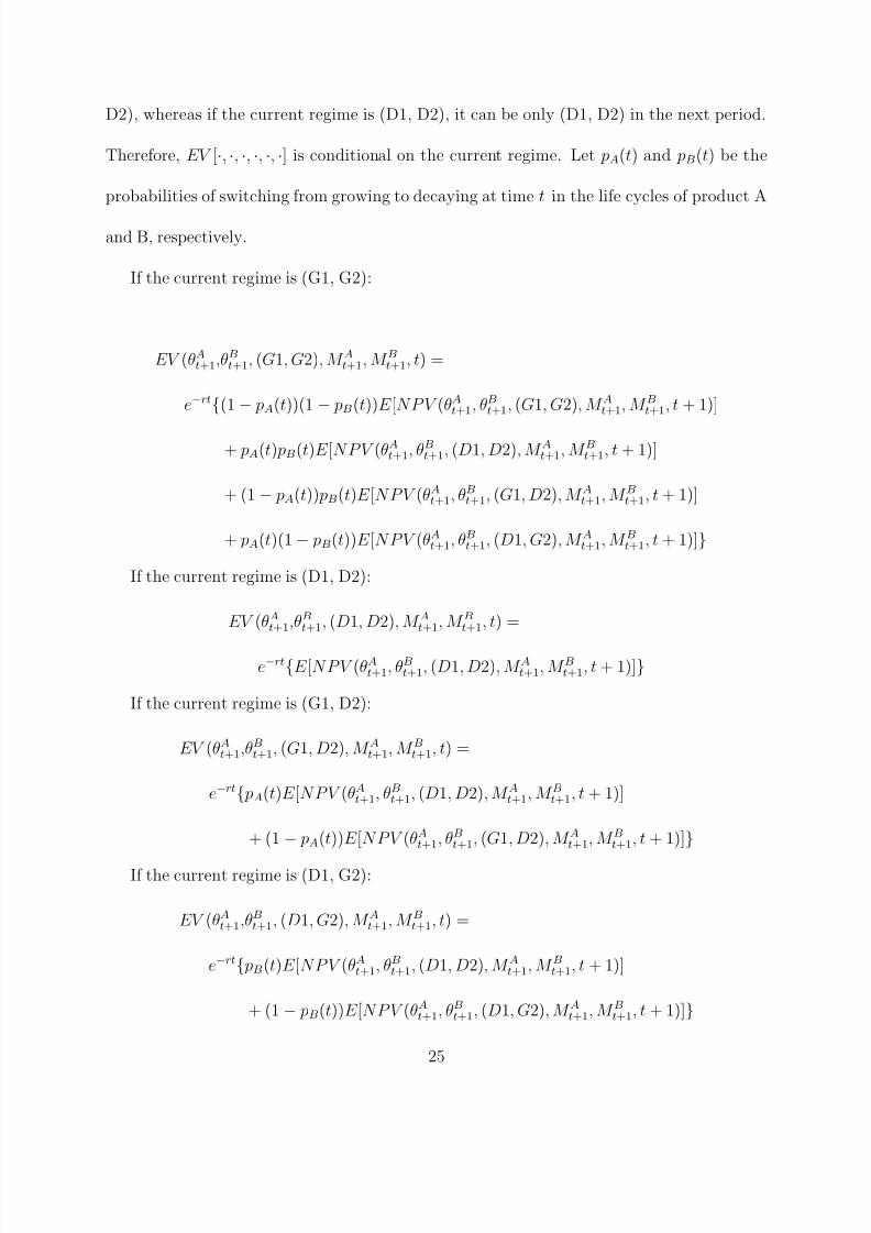
D2), whereas if the current regime is (D1, D2), it can be only (D1, D2) in the next period.
Therefore, EV [·, ·, ·, ·, ·, ·] is conditional on the current regime. Let pA(t) and pB(t) be the
probabilities of switching from growing to decaying at time t in the life cycles of product A
and B, respectively.
If the current regime is (G1, G2):
EV (θAt+1,θBt+1, (G1, G2), M At+1, M Bt+1, t) =
e−rt{(1 − pA(t))(1 − pB(t))E [NP V (θAt+1, θBt+1, (G1, G2), M At+1, M Bt+1, t + 1)]
+ pA(t) pB(t)E [N P V (θAt+1, θBt+1, (D1, D2), M At+1, M Bt+1, t + 1)]
+ (1 − pA(t)) pB(t)E [N P V (θAt+1, θBt+1, (G1, D2), M At+1, M Bt+1, t + 1)]
+ pA(t)(1 − pB(t))E [N P V (θAt+1, θBt+1, (D1, G2), M At+1, M Bt+1, t + 1)]}
If the current regime is (D1, D2):
EV (θAt+1,θBt+1, (D1, D2), M At+1, M Bt+1, t) =
e−rt{E [N P V (θAt+1, θBt+1, (D1, D2), M At+1, M Bt+1, t + 1)]}
If the current regime is (G1, D2):
EV (θAt+1,θBt+1, (G1, D2), M At+1, M Bt+1, t) =
e−rt{ pA(t)E [N P V (θAt+1, θBt+1, (D1, D2), M At+1, M Bt+1, t + 1)]
+ (1 − pA(t))E [N P V (θAt+1, θBt+1, (G1, D2), M At+1, M Bt+1, t + 1)]}
If the current regime is (D1, G2):
EV (θAt+1,θBt+1, (D1, G2), M At+1, M Bt+1, t) =
e−rt{ pB(t)E [NP V (θAt+1, θBt+1, (D1, D2), M At+1, M Bt+1, t + 1)]
+ (1 − pB(t))E [NP V (θAt+1, θBt+1, (D1, G2), M At+1, M Bt+1, t + 1)]}
25

7/17/2019 Flexibility on Switching Option
http://slidepdf.com/reader/full/flexibility-on-switching-option 28/38
We assume switching probabilities are from a cumulative normal distribution function
of the time elapsed from the introduction of product. The expectation of NPV can be
computed as the product of conditional branch probabilities and their corresponding NPV.
The backward dynamic programming approach is carried out from the terminal layer to the
root node of the lattice. At the root node, the discounted expected value of the whole project
can be found for each possible combination of initial capacity levels. The initial capacity
level that maximizes the NPV values of project at the root node is an optimal capacity level.
4 NUMERICAL EXAMPLE
We present a numerical example of a manufacturing system producing two products to
meet random demand streams over a given horizon. We investigate the impact of various
parameters of the manufacturing system on the value of manufacturing flexibility. The
project spans over a 5 years period, during which time the flexible capacity manufacturing
system optimally determines the production levels for two products at every period, whereas
the fixed capacity system has a single chance to set the capacity levels at time 0, so as
to maximize the total discounted expected profit over the horizon. Both products are in
growing regime at the beginning of the project and may switch into decaying regime anytime
with probability drawn from normal distribution with the mean 2.8 years and the variance
0.5 years for product A and the mean 2.3 years and the variance 0.5 years for product B,
respectively.
The capacity level for product A and B can be adjusted among 10 equally spaced levels
with a unit increment in capacity amounting to production of 2 additional units of corre-
26

7/17/2019 Flexibility on Switching Option
http://slidepdf.com/reader/full/flexibility-on-switching-option 29/38
sponding product per period. In each period the maximum capacity levels M it for product
A and B are sought for among 100 possible combinations of capacity levels to maximize the
profit in the current period as well as the discounted expected profit in the remaining future.
Regular capacity level of type A is 75% of the maximum capacity level; types B is 80% of
the maximum capacity level. The parameters used in the example related to the demand
evolution are given below:
ρ1 = 0.60, (µAg , σA
g ) = ( 36%, 30%),
ρ2 = 0.55, (µAd , σA
d ) = (-18%, 20%),
ρ3 = -0.45, (µBg , σB
g ) = ( 24%, 20%),
ρ4 = -0.50, (µBd , σB
d ) = (-24%, 25%).
The riskless rate of interest is 10% and the initial monthly demand of product A is 10 and
product B is 12. Unit prices of product A and B are $30,000 and $25,000, respectively. Cost
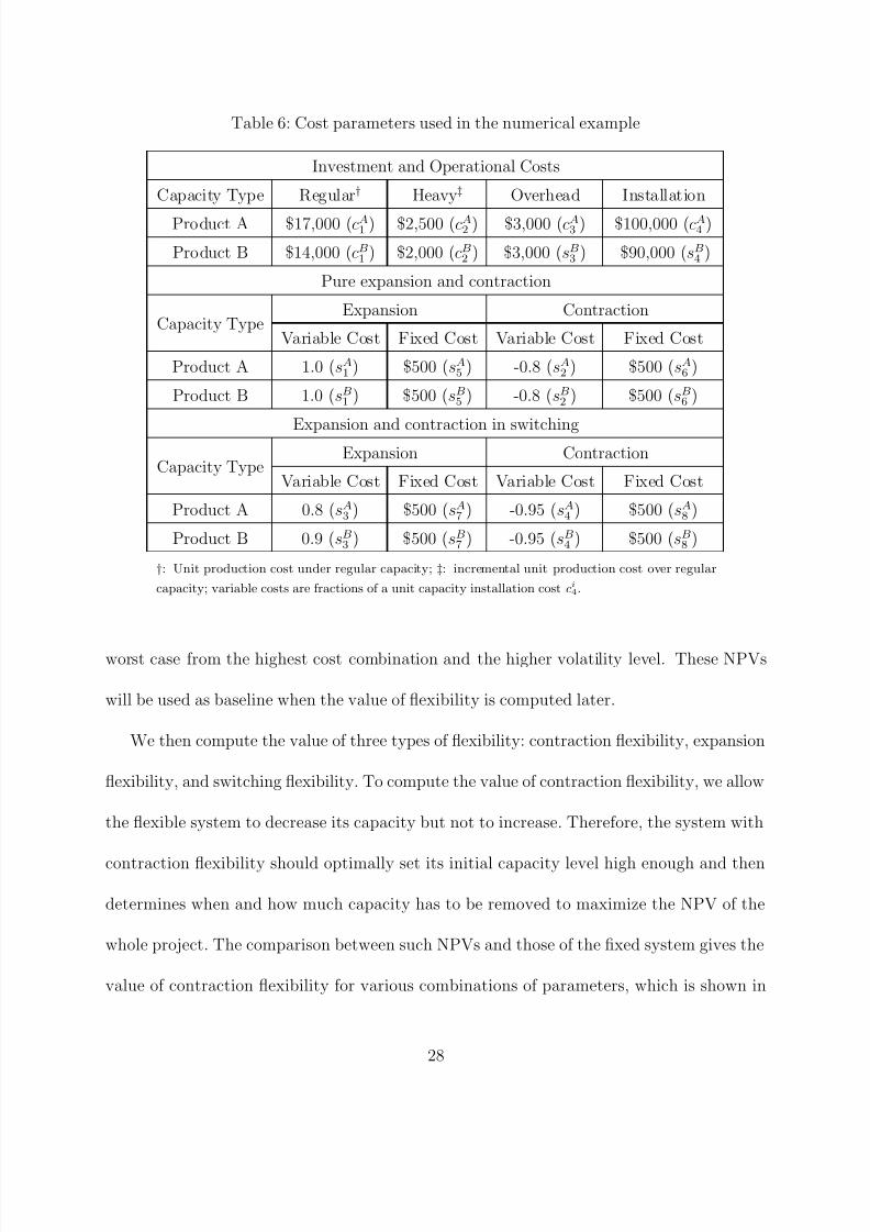
parameters associated with production and capacity adjustment are given in Table 6.
The first experiment is carried out to compute the value of different types of manu-
facturing flexibility – expansion, contraction, switching, and the combination of all three
flexibilities – with changing values for the cost parameters such as the overhead cost of unit
capacity for product A (cA3 ) and B (cB3 ), the unit capacity installation cost for product A
(cA4 ) and B (cB4 ), and the volatility level of product A in its growing regime. The results are
presented in Table 7 through Table 11.
Table 7 shows the net present value (NPV) of the fixed capacity system for total 18 com-
binations of 5 parameters. For every combination, the initial capacity level is set optimally
to maximize the NPV at time 0. As clearly shown, the NPV decreases as the unit capacity
installation cost and/or the unit capacity overhead cost increase. The maximum NPV, which
is from the lowest cost combination and the lower volatility level, is 25% higher than the
27
7/17/2019 Flexibility on Switching Option
http://slidepdf.com/reader/full/flexibility-on-switching-option 30/38
Table 6: Cost parameters used in the numerical example
Investment and Operational Costs
Capacity Type Regular† Heavy‡ Overhead Installation
Product A $17,000 (cA1 ) $2,500 (cA2 ) $3,000 (cA3 ) $100,000 (cA4 )
Product B $14,000 (cB1 ) $2,000 (cB2 ) $3,000 (sB3 ) $90,000 (sB4 )
Pure expansion and contraction
Capacity TypeExpansion Contraction
Variable Cost Fixed Cost Variable Cost Fixed Cost
Product A 1.0 (sA1 ) $500 (sA5 ) -0.8 (sA2 ) $500 (sA6 )
Product B 1.0 (sB1 ) $500 (sB5 ) -0.8 (sB2 ) $500 (sB6 )
Expansion and contraction in switching
Capacity TypeExpansion Contraction
Variable Cost Fixed Cost Variable Cost Fixed Cost
Product A 0.8 (sA3 ) $500 (sA7 ) -0.95 (sA4 ) $500 (sA8 )
Product B 0.9 (sB3 ) $500 (sB7 ) -0.95 (sB4 ) $500 (sB8 )
†: Unit production cost under regular capacity; ‡: incremental unit production cost over regular
capacity; variable costs are fractions of a unit capacity installation cost ci4.
worst case from the highest cost combination and the higher volatility level. These NPVs
will be used as baseline when the value of flexibility is computed later.
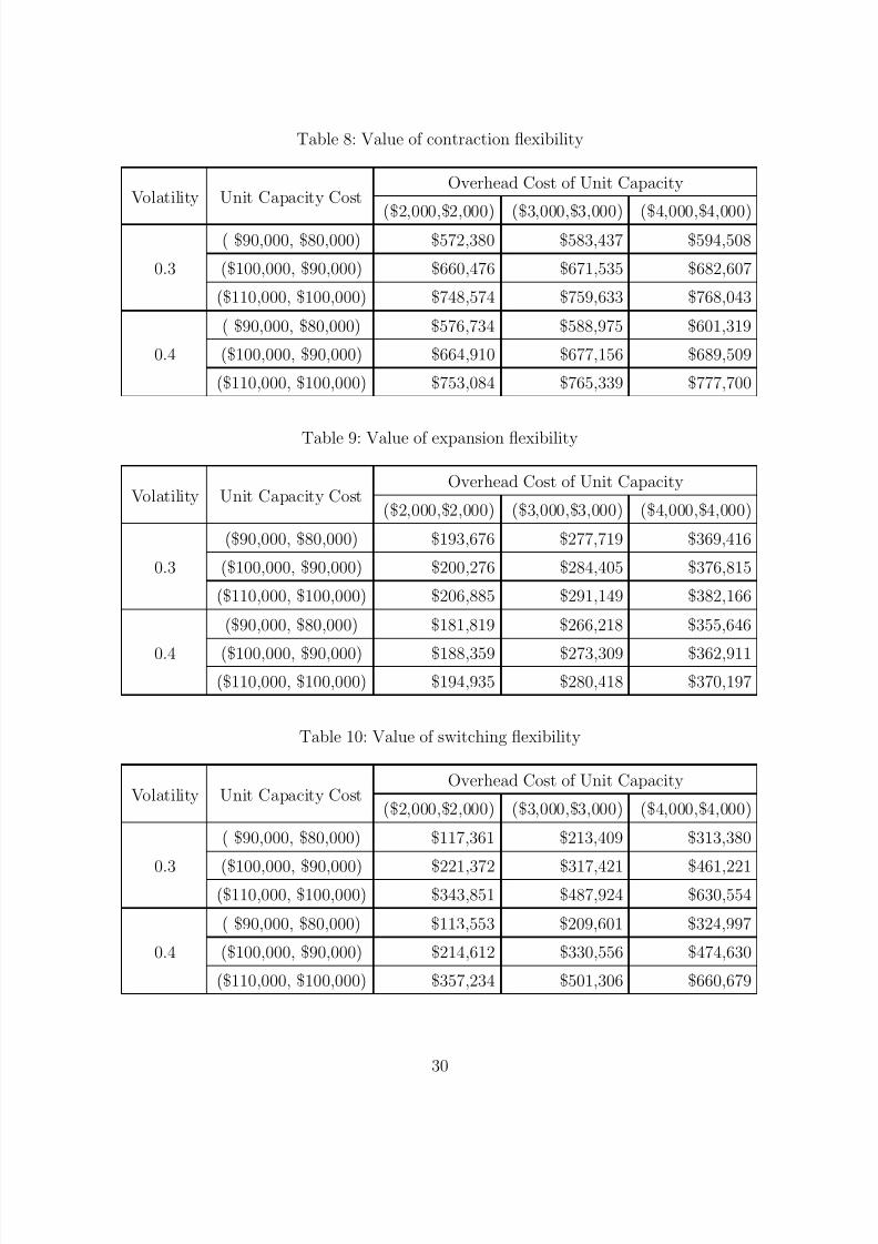
We then compute the value of three types of flexibility: contraction flexibility, expansion
flexibility, and switching flexibility. To compute the value of contraction flexibility, we allow
the flexible system to decrease its capacity but not to increase. Therefore, the system with
contraction flexibility should optimally set its initial capacity level high enough and then
determines when and how much capacity has to be removed to maximize the NPV of the
whole project. The comparison between such NPVs and those of the fixed system gives the
value of contraction flexibility for various combinations of parameters, which is shown in
28

7/17/2019 Flexibility on Switching Option
http://slidepdf.com/reader/full/flexibility-on-switching-option 31/38
Table 7: NVP of Fixed System
Volatility Unit Capacity CostOverhead Cost of Unit Capacity
($2,000,$2,000) ($3,000,$3,000) ($4,000,$4,000)
( $90,000, $80,000) $12,179,293 $11,218,808 $10,258,323
0.3 ($100,000, $90,000) $11,979,293 $11,018,808 $10,058,323
($110,000, $100,000) $11,779,293 $10,818,808 $9,858,323
( $90,000, $80,000) $12,107,645 $11,147,158 $10,186,670
0.4 ($100,000, $90,000) $11,907,645 $10,947,158 $9,986,670
($110,000, $100,000) $11,707,645 $10,747,158 $9,786,670
Table 8. Similar experiments find the value of expansion flexibility shown in Table 9 and the
value of switching flexibility shown in Table 10.
Interesting patterns are observed. First, the value of switching flexibility is almost equally
sensitive to the capacity installation cost and to the capacity overhead cost, whereas the value
of contraction flexibility is sensitive only to the capacity installation cost and the value of
expansion capacity is sensitive only to the capacity overhead cost. Due to its sensitivity
to both costs, it sways over a wider range: its lowest value is $113,553 and its highest
value is $660,679. Second, as the volatility of product A in the growing regime increases
from 30% to 40%, the value of switching flexibility decreases in three instances, where
both the installation and the overhead cost are low: {($2,000,$2,000),($90,000,$80,000)},
{($2,000,$2,000),($100,000,$90,000)
}, and
{($3,000,$3,000),($90,000,$80,000)
}). High volatil-
ity typically implies high value of flexibility. However, in the three instances, the optimal
initial capacity level of is 8 for product A and 9 for product B, which are close to the maxi-
mum capacity level that the flexible system can take, and the flexible system has little room
to shift its capacity between the two products (This is also why the value of contraction
29
7/17/2019 Flexibility on Switching Option
http://slidepdf.com/reader/full/flexibility-on-switching-option 32/38
Table 8: Value of contraction flexibility
Volatility Unit Capacity CostOverhead Cost of Unit Capacity
($2,000,$2,000) ($3,000,$3,000) ($4,000,$4,000)( $90,000, $80,000) $572,380 $583,437 $594,508
0.3 ($100,000, $90,000) $660,476 $671,535 $682,607
($110,000, $100,000) $748,574 $759,633 $768,043
( $90,000, $80,000) $576,734 $588,975 $601,319
0.4 ($100,000, $90,000) $664,910 $677,156 $689,509
($110,000, $100,000) $753,084 $765,339 $777,700
Table 9: Value of expansion flexibility
Volatility Unit Capacity CostOverhead Cost of Unit Capacity
($2,000,$2,000) ($3,000,$3,000) ($4,000,$4,000)
($90,000, $80,000) $193,676 $277,719 $369,416
0.3 ($100,000, $90,000) $200,276 $284,405 $376,815
($110,000, $100,000) $206,885 $291,149 $382,166
($90,000, $80,000) $181,819 $266,218 $355,646
0.4 ($100,000, $90,000) $188,359 $273,309 $362,911($110,000, $100,000) $194,935 $280,418 $370,197
Table 10: Value of switching flexibility
Volatility Unit Capacity CostOverhead Cost of Unit Capacity
($2,000,$2,000) ($3,000,$3,000) ($4,000,$4,000)
( $90,000, $80,000) $117,361 $213,409 $313,380
0.3 ($100,000, $90,000) $221,372 $317,421 $461,221($110,000, $100,000) $343,851 $487,924 $630,554
( $90,000, $80,000) $113,553 $209,601 $324,997
0.4 ($100,000, $90,000) $214,612 $330,556 $474,630
($110,000, $100,000) $357,234 $501,306 $660,679
30

7/17/2019 Flexibility on Switching Option
http://slidepdf.com/reader/full/flexibility-on-switching-option 33/38
flexibility is much higher than that of expansion flexibility). Third, the value of contraction
flexibility is much more sensitive to the capacity installation cost than to the overhead cost,
whereas the value of expansion flexibility is much more sensitive to the overhead cost than
to the installation cost. This is quite counter-intuitive in that one would guess that the
capability of reducing the capacity is more and more important as the cost of maintaining
capacity becomes more costly. Since two types of flexibility are sensitive to two different
cost parameters, the total flexibility becomes sensitive to the overhead and installation cost
to more or less the same degree.
When the system has the complete freedom in adjusting the capacity levels, the value
of flexibility is more than any of the restricted flexibilities. The total value of flexibility is
computed with the full flexibility and given in Table 11. Notice that the value of complete
flexibility is not necessarily equal to the sum of the values of three flexibility types.
Table 11: Total value of flexibility
Volatility Unit Capacity CostOverhead Cost of Unit Capacity
($2,000,$2,000) ($3,000,$3,000) ($4,000,$4,000)
( $90,000, $80,000) $955,449 $1,042,041 $1,130,198
0.3 ($100,000, $90,000) $1,092,556 $1,179,742 $1,268,591
($110,000, $100,000) $1,254,974 $1,345,924 $1,441,864
( $90,000, $80,000) $962,795 $1,049,542 $1,140,703
0.4 ($100,000, $90,000) $1,101,649 $1,189,665 $1,284,516
($110,000, $100,000) $1,264,983 $1,361,322 $1,461,855
As expected, the value of flexibility increases as the cost of capacity (installation and
maintenance cost) increases. The maximum value of flexibility among all 18 combinations of
various cost parameters is 53% more than the lowest value and amounts to 15% of the NPV
31

7/17/2019 Flexibility on Switching Option
http://slidepdf.com/reader/full/flexibility-on-switching-option 34/38
of the fixed capacity system.
Lastly, we investigate how the value of flexibility reacts to changes in the regime switching
mean and volatility. The mean and volatility of regime switching process are presented in
years in Table 12 along with the value of flexibility for each combination of the mean and the
volatility. It is intuitive to have the value of flexibility increasing as the mean of switching
Table 12: Total Value of Flexibility with Product Life cycles
Volatility Switch MeanVolatility of Switching Distribution
(0.25, 0.25) (0.5, 0.5) (0.75, 0.75)
(1.2, 1.1) $1,001,769 $987,964 $975,530
0.3 (2.8, 2.3) $1,185,993 $1,179,742 $1,174,355
(3.8, 3.6) $1,252,331 $1,249,066 $1,246,279
(1.2, 1.1) $1,011,410 $998,504 $987,007
0.4 (2.8, 2.3) $1,196,451 $1,189,665 $1,183,897
(3.8, 3.6) $1,277,420 $1,273,168 $1,269,557
distribution increases since the future demands are more likely to get larger as the products
stay in their growing regime longer. As a result the optimal level of capacity in the future is
higher than that of today and the expansion flexibility becomes more valuable. The reaction
of the value of flexibility to the uncertainty in the future demand is interesting. The value of
flexibility increases as the volatility of the future demand increases as we expect. However,
it decreases as the variance of the regime switching distribution increases. Considering that
both the volatility of future demand and the variance of the regime switching distribution
represent the different dimensions of uncertainty, it might seem somewhat contradictory. One
possible explanation for this is that the larger variance of the regime switching spreads the
32

7/17/2019 Flexibility on Switching Option
http://slidepdf.com/reader/full/flexibility-on-switching-option 35/38
peak demands for the two products over a wider range in time and the manufacturing system
would not dramatically change its capacity over time. Therefore, the value of flexibility is
reduced.
5 CONCLUSIONS
Unlike financial options, the lifespan of a real option such as manufacturing flexibility is typ-
ically over multiple years, which makes the assumption of stationarity unrealistic. Moreover,
it is often the case that a manufacturing system produces multiple products and the way to
exercise flexibility embedded in the system requires complicated steps. As a result it is not
possible to use analytical solutions developed for financial option valuation in the valuation
of complex manufacturing flexibility.
In this paper we construct a lattice for two correlated variables with regime switch-
ing. Transformation to obtain uncorrelated processes allows us to build a lattice using the
traditional moment matching approach. We employ a dynamic programming approach to
valuation of the manufacturing flexibility. The numerical studies on an example hint many
interesting aspects of manufacturing flexibility as discussed in Section 4. However, extensive
studies are required before generalizing our observations.
Due to the exponentially increasing number of node in the lattice as the number of
variables increases, it still remains a challenge to study manufacturing flexibility with more
than 2 variables. The approach presented in the paper would not support the case with
more than 2 variables and a general lattice framework dealing with n(n > 2) variables can
be found in Wahab and Lee [21].
33

7/17/2019 Flexibility on Switching Option
http://slidepdf.com/reader/full/flexibility-on-switching-option 36/38
References
[1] F. Bass. A new product growth model for consumer durables. Management Science ,
15:215–227, 1969.
[2] J. Bengtsson. Manufacturing flexibility and real options: A review. International Jour-
nal of Production Economic , 74:213–224, 2001.
[3] N. P. Bollen. Valuing options in regime-switching models. Journal of Derivatives , 6:38–
49, 1998.
[4] N. P. Bollen. Real option and product life cycle. Management Science , 45(5):670–684,
1999.
[5] P. P. Boyle. A lattice framework for option pricing with two state variables. Journal of
Financial and Quantitative Analysis , 23:1–12, 1988.
[6] P. P. Boyle, J. Evnine, and S. Gibbs. Numerical evaluation of multivariate contingent
claims. The Review of Financial Studies , 2(2):241–250, 1989.
[7] M. Brennan and E. Schwartz. Evaluating natural resource investment. Journal of
Business , 58:135–157, 1985.
[8] J. Cox, S. Ross, and M. Rubinstein. Option pricing: A simplified approach. Journal of
Financial Economics , 7:229–264, 1979.
[9] H. He and R. Pindyck. Investment in flexible production capacity. Journal of Dynamics
and Control , 16:575–599, 1992.
34
7/17/2019 Flexibility on Switching Option
http://slidepdf.com/reader/full/flexibility-on-switching-option 37/38
[10] J. Hull. Options, Futures, and Other Derivatives . Prentice-Hall, New Jersey, 2002.
[11] J. Hull and A. White. Valuing derivative securities using the explicit finite difference
method. Journal of Financial and Quantitative Analysis , 25:87–100, 1990.
[12] N. Kulatilaka. Valuing the flexibility of flexible manufacturing system. IEEE Transac-
tions on Engineering Management , 35:250–257, 1988.
[13] S. Majd and R. Pindyck. Time to build, option value, and investment decision. Journal
of Financial Economics , 19:7–27, 1987.
[14] R. McDonald and D. Siegel. Investment and the valuation of firms when there is an
option to shut down. International Economic Review , 26:331–349, 1985.
[15] R. McDonald and D. Siegel. The value of waiting to invest. The Quarterly Journal of
Economics , 101:707–727, 1986.
[16] J. Norton and F. Bass. A diffusion theory model od adoption and substitution for
successive generations of high-technology products. Management Science , 41:713–721,
1987.
[17] R. Pindyck. Irreversible investment, capacity choice, and the value of the firm. The
American Economic Review , 78:969–985, 1988.
[18] A. Sethi and S. Sethi. Flexibility in manufacturing: A survey. The International Journal
of Flexible Manufacturing Systems , 2:289–328, 1990.
[19] G. Tannos. Capital budgeting for volume flexible equipment. Decision Science , 27:157–
184, 1996.
35
7/17/2019 Flexibility on Switching Option
http://slidepdf.com/reader/full/flexibility-on-switching-option 38/38
[20] A. Triantis and J. Hodder. Valuing flexibility as a complex option. The Journal of
Finance , 45:549–565, 1990.
[21] M. Wahab and C.-G. Lee. A lattice approach to a multi-variate contingent claims with
regime switching. Technical Report (MIE-OR TR2005-03), Department of Mechanical
and Industrial Engineering at the Univefsity of Toronto, 2005.