flexible learning approach to physics ÊÊÊ module m5.5 further integration … › physics ›...

F L E X I B L E L E A R N I N G A P P R O A C H T O P H Y S I C S

FLAP M5.5 Further IntegrationCOPYRIGHT © 1998 THE OPEN UNIVERSITY S570 V1.1

Module M5.5 Further integration1 Opening items

1.1 Module introduction

1.2 Fast track questions

1.3 Ready to study?

2 Further techniques of integration

2.1 Partial fractions

2.2 Completing the square

2.3 Splitting the numerator

2.4 Substitutions involving hyperbolic functions

2.5 Using trigonometric identities

2.6 Reduction formulae

2.7 Mixed examples

3 Some definite integrals

3.1 Integrals with an infinite upper or lower limit

3.2 Gaussian integrals

3.3 Line integrals

4 Closing items

4.1 Module summary

4.2 Achievements

4.3 Exit test

Exit module


1 Opening items1.1 Module introductionThis module discusses in depth a range of techniques which will enable you to evaluate a wide range ofintegrals. Such a detailed treatment may not be relevant to your course of study, and you are therefore advised toconsult your tutor before working through the module. You should be prepared to spend more time than for theother FLAP modules if you are advised to read all the material.

In Section 2 we discuss several ingenious tricks which you can combine with methods such as integration byparts and integration by substitution in order to evaluate a very wide range of integrals. Some of these tricks(partial fractions, completing the square and splitting the numerator) involve algebraic manipulation of theintegrand, while others make use of trigonometric identities to simplify integrals of powers of trigonometricfunctions. We also discuss some particularly useful substitutions involving hyperbolic functions.

Subsection 3.1 deals with certain types of improper integral1 1those with an infinite upper or lower limit.We will explain there how to define and evaluate these. Subsection 3.2 discusses some integrals of this sortknown as Gaussian integrals, which arise very often in physics (in quantum mechanics and in the kinetic theoryof gases, for example). We show how these can all be evaluated in terms of the basic Gaussian integral

exp(−x2 ) dx0

∞

∫ ☞.


Finally, in Subsection 3.3, we introduce and explain the idea of a line integral1 1an integral of the form

F(r)⋅dr

ra

rb

∫ . Integrals of this sort arise in calculating the work done by a force, for example, or the electrostatic

potential difference between two points in a region of space where there is an electric field.

You may occasionally find that your answers to the exercises differ from ours. This may be because your answeris in a slightly different form; for example, you may have written loge x (x − 1) where we have written12 loge x − 1

2 loge (x − 1) . If you cannot tell if your expression for an indefinite integral is the same as ours, youcan always check your answer by differentiating it.

Study comment Having read the introduction you may feel that you are already familiar with the material covered by thismodule and that you do not need to study it. If so, try the Fast track questions given in Subsection 1.2. If not, proceeddirectly to Ready to study? in Subsection 1.3.


1.2 Fast track questions

Study comment Can you answer the following Fast track questions?. If you answer the questions successfully you needonly glance through the module before looking at the Module summary (Subsection 4.1) and the Achievements listed inSubsection 4.2. If you are sure that you can meet each of these achievements, try the Exit test in Subsection 4.3. If you havedifficulty with only one or two of the questions you should follow the guidance given in the answers and read the relevantparts of the module. However, if you have difficulty with more than two of the Exit questions you are strongly advised tostudy the whole module.

Question F1

Find the integrals (a) x − 1

4x2 − 1dx⌠

⌡, (b)

1

1 + 8x − 4x2⌠⌡

dx


Question F2

Evaluate the definite integral x + 3

x + 2( )2 x + 1( )0

∞⌠⌡

dx ☞

Question F3

Evaluate the definite integral

exp(−3x2 + 4x) dx−∞

∞∫ 4given that4 exp(−y2 ) dy

−∞

∞∫ = π .


Study comment Having seen the Fast track questions you may feel that it would be wiser to follow the normal routethrough the module and to proceed directly to Ready to study? in Subsection 1.3.

Alternatively, you may still be sufficiently comfortable with the material covered by the module to proceed directly to theClosing items.


1.3 Ready to study?

Study comment

In order to study this module, you will need to be familiar with the following terms: completing the square, definite integral,even function, hyperbolic function, improper integral, integrand, integration by parts, integration by substitution, inversehyperbolic function, limits of integration, scalar product and vector. If you are uncertain of any of these terms, you canreview them now by referring to the Glossary which will indicate where in FLAP they are developed. In addition, you will

need to be familiar with standard integrals (such as xn∫ dx = xn +1

n + 1+ C ☞ and eax∫ dx = eax

a+ C ), and know how to

evaluate definite and indefinite integrals by the method of substitution, or by integration by parts. You will also need to befamiliar with trigonometric identities, and with the analogous identities involving hyperbolic functions. The following Readyto study questions will allow you to establish whether you need to review some of these topics before embarking on thismodule.

Mike Tinker

Mike Tinker

Mike Tinker

Mike Tinker

Mike Tinker

Mike Tinker

Mike Tinker

Mike Tinker

Mike Tinker


Question R1

The expression 1

x − 1+ 2

x + 2 can be written as a single fraction by putting

1x − 1

+ 2x + 2

= x + 2(x − 1)(x + 2)

+ 2(x − 1)(x − 1)(x + 2)

= (x + 2) + 2(x − 1)(x − 1)(x + 2)

= 3x

(x − 1)(x + 2)

Use a similar method to express the following as single fractions:

(a) 1

2(x − 3)− 1

2(x + 3), (b)

12 − x

+ x

3 + x2, (c)

59(x − 1)

− 59(x + 2)

− 23(x + 2)2

Question R2

Write the following quadratic functions in completed square form: (a) 3x2 − 12x +16,4(b) 3 − 4x − 2x2


Question R3

(a) If y = cos1(2x), express sin41x in terms of y.

(b) If y = cosh1(2x), express sinh41x in terms of y.

Question R4

Find the indefinite integrals:

(a) 1

2 + 3x⌠⌡

dx ,4(b) 1

4 + 9x2⌠⌡

dx ,4(c) 1

25 − 4x2⌠⌡

dx .


Question R5

Evaluate the definite integrals:

(a) x0

π

∫ sin (3x) dx ,4(b) x0

1

∫ 1 + 4x2 dx .

Question R6

Define the hyperbolic functions cosh1x and sinh1x , and use your definitions to prove the identitycosh21x − sinh21x = 1.


Question R7

(a) What are the derivatives of cosh1x and sinh1x? Use these derivatives, and the quotient rule, to find thederivative of tanh1x.

(b) Find the integrals cosh (2x)∫ dx and sinh (x 3)∫ dx .

Question R8

If r is the vector xi + y1j + zk, a is the vector 2i − k and b is the vector 2i − 21j + k, find an expression for(a1·1b)(b1·1r) in terms of x, y and z.


2 Further techniques of integration

2.1 Partial fractions

Suppose that we want to find the integral 1

(x + 1)(x + 2)⌠⌡

dx . The integrand does not seem to be a particularly

complicated function of x. Yet this is not an integral that can immediately be related to a standard integral, norwill integration by parts work (as you will find if you try!), nor is it easy to find a substitution that will simplifythe integral.

However, this integral can in fact be found quite easily if we first split the integrand into its partial fractions.☞ To do this, we write

1(x + 1)(x + 2)

= a

x + 1+ b

x + 2(1)

where a and b are constants that we will need to find. Adding together the two fractions on the right-hand side ofEquation 1 gives us


1(x + 1)(x + 2)

= (a + b)x + 2a + b

(x + 1)(x + 2)

from which we deduce that a + b = 0 and 2a + b = 1, so that a = 1, b = −1. Thus we have the identity

1(x + 1)(x + 2)

= 1x + 1

− 1x + 2

☞

It follows that

1(x + 1)(x + 2)

⌠⌡

dx = 1x + 1

⌠⌡

dx − 1x + 2

⌠⌡

dx = loge (x + 1) − loge (x + 2) + C ☞

The method we have used here to find 1

(x + 1)(x + 2)⌠⌡

dx can be applied to a wide variety of integrals of

fractions whose denominators can be factorized. Here is a slightly more complicated example.


Example 1

Find x

x2 + x − 6⌠⌡

dx .

Solution4Since the denominator is not already factorized, we must first find its factors, which are (x − 2) and

(x + 3). We now express x

x2 + x − 6= x

(x − 2)(x + 3) in partial fractions. We write

x

(x − 2)(x + 3)= a

x − 2+ b

x + 3= (a + b)x + 3a − 2b

(x − 2)(x + 3)

from which we deduce that a + b = 1 and 3a − 2b = 0, i.e. a = 2/5 and b = 3/5.


Thusx

x2 + x − 6= 2

5(x − 2)+ 3

5(x + 3)

so that x

x2 + x − 6⌠⌡

dx = 25

1x − 2

⌠⌡

dx + 35

1x + 3

⌠⌡

dx = 25

loge (x − 2) + 35

loge (x + 3) + C

This example shows that using partial fractions to evaluate integrals generally involves three steps:

Step 14Factorize the denominator of the integrand (if necessary).

Step 24Express the integrand in terms of partial fractions.

Step 34Integrate each partial fraction.

Practise these steps by doing the following question.

Question T1

Find the integral 1

9 − 4x2⌠⌡

dx .4❏ ☞


The three steps described above apply equally well if there is a repeated factor in the denominator of theintegrand. For example, consider the integral

1x3 − 2x2 + x

⌠⌡

dx

The denominator here is x3 − 2x2 + x = x(x02 − 2x + 1) = x(x − 1)2, which has a repeated factor (x –1).We now write

1

x(x − 1)2 = a

x+ b

x − 1

A term for ( x −1)}

+ d

(x − 1)2

A term for ( x −1)2

674 84

= a + b( )x2 + d − 2a − b( )x + a

x(x − 1)2

(and notice that we have included a term for (x – 1) and a term for (x – 1)2)

so that a + b = 0, d − 2a − b = 0, and a = 1, i.e. a = 1, b = −1, d = 1.

So1

x3 − 2x2 + x= 1

x− 1

x − 1+ 1

(x − 1)2(2)


✦

Find 1

x3 − 2x2 + x⌠⌡

dx .

Partial fractions can also often be used to integrate a fraction even if its denominator does not factorizecompletely into real linear factors, as in the following example.

Example 2

Find the integral x + 3

(x − 1)(x2 + 1)⌠⌡

dx

Solution4We cannot factorize the quadratic factor (x2 + 1). So, to express the integrand in terms of partialfractions, we must first write it in the form

x + 3

(x − 1)(x2 + 1)= a

x − 1+ bx + d

x2 + 1

Two constants forthe quadratic factor

678

= (a + b)x2 + (d − b)x + a − d

(x − 1)(x2 + 1)

(and notice that the term corresponding to the factor (x2 + 1) includes two unknown constants) from which itfollows that a + b = 0, d − b = 1 and a − d = 3, i.e. a = 2, b = −2, d = −1.


Sox + 3

(x − 1)(x2 + 1)⌠⌡

dx = 2x − 1

⌠⌡

dx − 2x + 1x2 + 1

⌠⌡

dx (3)

The first integral on the right-hand side of Equation 3 is equal to 21loge1(x − 1) + C. To evaluate the second

integral, we split it into two, and write it as 2x

x2 + 1⌠⌡

dx + 1x2 + 1

⌠⌡

dx . With the substitution u = x2 + 1, we

quickly find that 2x

x2 + 1⌠⌡

dx = loge (x2 + 1) + C , while 1

x2 + 1⌠⌡

dx is a standard integral, equal to arctan1x + C.

Substituting these results into Equation 3 gives usx + 3

(x − 1)(x2 + 1)⌠⌡

dx = 2 loge (x − 1) − loge (x2 + 1) − arctan x + C4❏ ☞


Question T2

Find the integral 3x2 + 11

(x − 3)(2x2 + 1)⌠⌡

dx .4❏

The technique of splitting the integrand into partial fractions will enable you to find many integrals of the formp(x)q(x)

⌠⌡

dx , where p(x) and q(x) are both polynomials in x. However, it clearly will not be of any use unless q(x)

factorizes, at least partly. What can we do if q(x) does not factorize at all? This case is discussed in the next twosubsections.


2.2 Completing the square

If you are asked to find the integral 1

x2 + 4x + 8⌠⌡

dx , your response may now be to try writing the integrand in

terms of partial fractions. If you try this, you will quickly find that the quadratic equation x02 + 4x + 8 = 0 has no

real roots, so that we cannot factorize the integrand, and partial fractions are of no use. ☞

To see how to proceed with an integral of this sort, recall that there are integrals similar to this which you do

know how to evaluate; for example, the integral 1

x2 + 4⌠⌡

dx . This also has the property that its integrand does

not factorize. However it can be quickly evaluated by means of the substitution x = 21tan1u. Then x2 + 4 = 4

sec21u, and dx = 21sec21u du, so that the integral becomes

12∫ du = 1

2 u + C = 12 arctan (x 2) + C

We can make the integral1

x2 + 4x + 8⌠⌡

dx look very much like the integral 1

x2 + 4⌠⌡

dx by the trick known as

completing the square, in which we write the denominator as the sum of two squared terms, one involving x andthe other a constant. In the case under consideration, it works as follows.


We notice that x02 + 4x = (x + 2)2 − 4, so that x2 + 4x + 8 = (x + 2)2 + 4.

Thus we have1

x2 + 4 + 8⌠⌡

dx = 1(x + 2)2 + 4

⌠⌡

dx

We now make the change of variables y = x + 2, so as to obtain1

x2 + 4x + 8⌠⌡

dx = 1y2 + 4

⌠⌡

dy

We have just evaluated the integral on the right-hand side here; it is equal to 12 arctan (y 2) + C .

Replacing y by x + 2, we finally find that1

x2 + 4x + 8⌠⌡

dx = 12 arctan[(x + 2) 2] + C

Here is a slightly more complicated example, which we will set out as a series of steps; you can follow thesewhen you do similar problems.


Example 3

Find the integral I = 12x2 + 6x + 5

⌠⌡

dx ☞

Solution4Step 14First, write the denominator in completed square form.

2x2 + 6x + 5 = 2(x2 + 3x) + 5 = 2 x + 3 2( )2 − 9 4[ ] + 5 = 2 x + 3 2( )2 + 1 2

So I = 12[x + (3 2)]2 + 1 2

⌠⌡

dx

Step 24Make the substitution y = x + 32

, then I = 12y2 + (1 2)

⌠⌡

dy

Step 34Make the substitution y = 12 tan u, then 2y2 + 1

2 = 12 sec2 u and dy = 1

2 sec2 u du . So

I = 1 21 2

⌠⌡

du = 1du = u + C∫ . ☞

Step 44Finally, express the integral in terms of x (using the fact that x + 32 = 1

2 tan u ),

I = u + C = arctan1(2y) + C = arctan1(2x + 3) + C.4❏


Question T3

Find the integral I = 13x2 − 6x + 7

⌠⌡

dx4❏

The technique of completing the square can also be used in conjunction with a substitution of the form

x = a1sin1u, where a is a constant; this enables us to find integrals such as I = 1

3 − 2x − x2⌠⌡

dx . To evaluate

this integral, we first write the quadratic expression appearing under the square root sign in completed squareform.

✦ Write 3 − 2x − x02 in completed square form.

So 1

3 − 2x − x2⌠⌡

dx = 1

4 − (x + 1)2

⌠⌡

dx . We now make the substitution y = x + 1; then the integral

becomes 1

4 − y2

⌠⌡

dy . This integral can easily be found by the substitution y = 21sin1u, so that dy = 21cos1u1du,


then

1

4 − y2

⌠⌡

dy = 1

4 − (2 sin u)2

⌠⌡

(2 cosu du)

= 12 cosu

⌠⌡

(2 cosu du) = 1du∫ = u + C = arcsin (y 2) + C

Replacing y by x + 1, we finally have

1

3 − 2x − x2⌠⌡

dx = arcsinx + 1

2

+ C

Here is another example, which again we will set out as a series of steps.


Example 4

Find the integral I = 1

6x − x2⌠⌡

dx .

Solution4Step 14Write 6x − x2 in completed square form:

6x − x02 = − (x02 − 6x) = −[(x − 3)2 − 9] = 9 − (x − 3)2

so I = 1

9 − (x − 3)2

⌠⌡

dx

Step 24Make the substitution y = x – 3; then I = 1

9 − y2

⌠⌡

dy

Step 34Make the substitution y = 31sin1u; then 9 − y2 = 31cos1u and

dy = 31cos1u1du. So I = 1du = u + C∫Step 44Express I in terms of x0:

I = u + C = arcsiny

3

+ C = arcsin

x − 33

+ C4❏


Question T4

Find the integral I = 1

9 + 8x − 2x2⌠⌡

dx .4❏

In this subsection, we have so far discussed only indefinite integrals. However the techniques presented here canjust as easily be used to evaluate definite integrals. You need only remember to transform the limits ofintegration appropriately in each of Steps 2 and 3; if you do this, there will be no need for Step 4.

Question T5

Evaluate 1

x2 − 6x + 253

7

⌠⌡

dx .4❏


2.3 Splitting the numeratorIn the previous subsection, you learnt how to find integrals where the integrand had a quadratic denominator thatdid not factorize, and had a constant in the numerator. Suppose the integrand had an expression linear in x in the

numerator, instead of a constant; for example, suppose you were required to integrate 2x + 3

x2 − 4x + 10.

How would you proceed here?

To see what to do in such a case, notice that we in fact already encountered an integral of this sort in Example 2,

where we had to find the integral 2x + 1x2 + 1

⌠⌡

dx . We evaluated it by writing it as the sum of the two integrals:

2x

x2 + 1⌠⌡

dx and 1

x2 + 1⌠⌡

dx . The first of these integrals could be easily evaluated, since the numerator is equal

to the derivative of the denominator; thus the substitution y = x2 + 1 enabled us to find it. The second could alsobe found, using the substitution x = tan1y.


We can apply the same idea to an integral such as 2x + 3

x2 − 4x + 10⌠⌡

dx . We write the numerator as the sum of two

terms, one which is a multiple of the derivative of the denominator and the other a constant. In the present case,this is easy to do. The derivative of x2 − 4x + 10 is 2x − 4, and clearly the numerator of our integral, 2x + 3, isequal to (2x − 4) + 7. So we write the integral as the sum of two integrals:

2x + 3x2 − 4x + 10

⌠⌡

dx = 2x − 4x2 − 4x + 10

⌠⌡

dx + 7x2 − 4x + 10

⌠⌡

dx (4)

The first integral on the right-hand side of Equation 4 can be found by means of the substitution y = x2 – 4x + 10,

and since d y = (2x − 4) d x, the integral becomes 1y

⌠⌡

dy = loge y + C = loge (x2 − 4x + 10) + C .

The second integral on the right-hand side of Equation 4 is of the sort you learnt to evaluate in Subsection 2.2.

The trick of writing

numerator = multiple of derivative of denominator + constant

is known as splitting the numerator. It involves only very simple algebra, as the following example shows.


Example 5

Split the numerator in the integral 2x + 1

3x2 + 4x + 2⌠⌡

dx .

Solution4The derivative of the denominator is d

dx(3x2 + 4x + 2) = 6x + 4 . So we write 2x + 1 = a(6x + 4) + b.

Equating the coefficients of x on both sides we find 2 = 6a, i.e. a =1/3, then equating the constant terms we find1 = 4a + b, so that b = −1/3.

Thus2x + 1

3x2 + 4x + 2⌠⌡

dx = 13

6x + 43x2 + 4x + 2

⌠⌡

dx − 13

13x2 + 4x + 2

⌠⌡

dx4❏

✦

Split the numerator in the integral 4 − x

x2 − x + 3⌠⌡

dx .


The technique of splitting the numerator can also be used to find integrals such as 1 − x

5 − 2x − x2⌠⌡

dx where the

integrand has the square root of a quadratic function of x in the denominator, and a linear function of x in thenumerator. To find this integral, we again write the numerator as a multiple of the derivative of the quadratic

function in the denominator [in this case d

dx(5 − 2x − x2 ) = −2 − 2x ], plus a constant; so that for this example

we have

1 − x numerator678

= a(−2 − 2x)

derivative of quadratic6 74 84

+ b constant}

Equating the coefficient of x, and the constant terms, on each side of this equation, we find a = 1/2, b = 2.

So1 − x

5 − 2x − x2⌠⌡

dx = 12

−2 − 2x

5 − 2x − x2⌠⌡

dx + 21

5 − 2x − x2⌠⌡

dx

The first integral on the right-hand side here can be found by the substitution y = 5 − 2x − x02, so thatdy = (−2 − 2x)1dx, and we have

12

−2 − 2x

5 − 2x − x2⌠⌡

dx = 12

1y

⌠⌡

dy = y + C = 5 − 2x − x2 + C


The second integral is one of those that you learnt to evaluate in Subsection 2.2. We complete the square in thedenominator, to obtain

1

5 − 2x − x2⌠⌡

dx = 1

6 − (x + 1)2

⌠⌡

dx

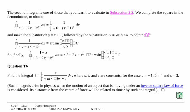
and make the substitution y = x + 1, followed by the substitution y = 6 sin u to obtain ☞1

5 − 2x − x2⌠⌡

dx = arcsinx + 1

6

+ C

So, finally,1 − x

5 − 2x − x2⌠⌡

dx = 5 − 2x − x2 + 2 arcsinx + 1

6

+ C

Question T6

Find the integral t = r

ar2 + br − c⌠⌡

dr , where a, b and c are constants, for the case a = − 1, b = 4 and c = 3.

(Such integrals arise in physics when the motion of an object that is moving under an inverse square law of forceis considered. Its distance r from the centre of force will be related to time t by such an integral.)4❏


2.4 Substitutions involving hyperbolic functionsYou should know how to evaluate integrals of the form: ☞

o 1

1 − x2dx⌠

⌡by means of the substitution x = sin1u ☞

o 1x2 + 1

dx⌠⌡

by means of the substitution x = tan1u ☞

o 1x2 − 1

dx⌠⌡

using partial fractions. ☞

Looking at this list, it may occur to you that there are two integrals which are missing from it, although they arevery similar to the integrals that do appear there: we have in mind the integrals

1

x2 + 1dx⌠

⌡4and4 1

x2 − 1dx⌠

⌡

In this subsection, we will show how to find these integrals (and many more which are related to them).


The integral 1

1 − x2dx⌠

⌡ is equal to arcsin1x + C; and one way to prove this is to make the substitution

x = sin1u. This substitution gets rid of the square root in the denominator, by virtue of the trigonometric identity

cos21u + sin21u =1; 1 − x2 becomes 1 − sin2 u = cosu , and this gives us a clue as to how to proceed with the

integral 1

1 + x2dx⌠

⌡. We recall that the hyperbolic functions cosh and sinh satisfy an identity very similar to

the one satisfied by cos and sin, but with a minus sign present, i.e. instead of cos21u + sin21u =1, we have

cosh21u – sinh21u =1. Thus we can get rid of the square root in 1 + x2 if we make the substitution x = sinh1u,

which gives 1 + x2 = 1 + sinh2 u = cosh u . Since d

du(sinh u) = cosh u , we also have dx = cosh1u du.

So, with the substitution x = sinh1u, the integral 1

1 + x2dx⌠

⌡ becomes very easy, and specifically we have

1

1 + x2dx⌠

⌡= 1

cosh u

cosh u du⌠

⌡= u + C

If x = sinh1u then u = arcsinh1x. Thus finally we have the result


1

x2 + 1dx⌠

⌡= arcsinh x + C (5) ☞

We can also exploit the identity cosh21u − sinh21u = 1 to evaluate the integral 1

x2 − 1dx⌠

⌡. The identity can be

rewritten in the form sinh u = cosh2 u − 1 , which suggests that we make the substitution x = cosh1u.

✦

What does the integral 1

x2 − 1dx⌠

⌡ become if we make the substitution x = cosh1u?

If x = cosh1u then u = arccosh1x, so that

1

x2 − 1dx⌠

⌡= arccosh x + C (6) ☞


Now that you know how to find the basic integrals 1

1 + x2dx⌠

⌡ and

1

x2 − 1dx⌠

⌡, you should not find it hard

to adapt the method to find integrals involving similar square roots. Here is an example.

Example 6

Find the integral 1

4 + 9x2⌠⌡

dx .

Solution4The experience that we gained in deriving Equation 5 suggests that we need to make a substitution of

the form x = a1sinh1u, where a is a suitably chosen constant. We choose a so that the identity cosh21u − sinh21u = 1

can be used to turn 4 + 9x2 into a multiple of cosh1u. If we substitute x = a1sinh1u into 4 + 9x2 , it becomes

4 + 9a2 sinh2 u which is equal to 21cosh1u if we choose 9a2 = 4, i.e. a = 2/3. So the required substitution is

x = (2/3)1sinh1u. We then have dx = (2/3)1cosh1u1du, and the integral becomes

1

4 + 9x2⌠⌡

dx = 12 cosh u

(2 3)cosh u du⌠⌡

= 13

⌠⌡

du = 13

u + C


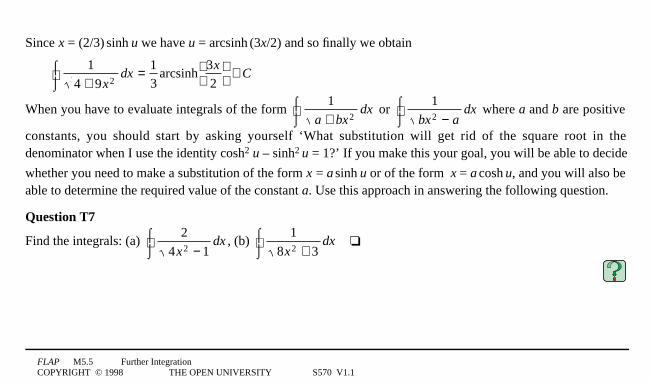
Since x = (2/3)1sinh1u we have u = arcsinh1(3x/2) and so finally we obtain

1

4 + 9x2⌠⌡

dx = 13

arcsinh3x

2

+ C

When you have to evaluate integrals of the form 1

a + bx2⌠⌡

dx or 1

bx2 − a⌠⌡

dx where a and b are positive

constants, you should start by asking yourself ‘What substitution will get rid of the square root in thedenominator when I use the identity cosh21u – sinh21u = 1?’ If you make this your goal, you will be able to decide

whether you need to make a substitution of the form x = a1sinh1u or of the form x = a1cosh1u, and you will also beable to determine the required value of the constant a. Use this approach in answering the following question.

Question T7

Find the integrals: (a) 2

4x2 − 1⌠⌡

dx , (b) 1

8x2 + 3⌠⌡

dx4❏


You can, of course, combine substitutions involving hyperbolic functions with the techniques of completing thesquare and splitting the numerator, in order to find even more integrals. For example, consider the integral

I = 1

4x + x2⌠⌡

dx .

✦ Write the quadratic function 4x + x2 in completed square form.

✦ What substitution should we make in order to evaluate 1

y2 − 4⌠⌡

dy ?


Question T8

Find the integral r

r2 + 2r − 2⌠⌡

dr . ☞

(Hint: This question requires you to split the numerator; this will leave you with two integrals, one to be foundby completing the square in the denominator and substituting a hyperbolic function.)4❏

We have seen that substitutions of hyperbolic functions enable us to find many integrals where the denominatorof the integrand is the square root of a quadratic function. They can also be used to integrate other functionsinvolving a square root of this sort, as in the following example.


Example 7

Find the integral x2 − 1∫ dx .

Solution4We first try the substitution x = cosh1u. Then x2 − 1 = sinh u and dx = sinh1u1du. So our integral

becomes sinh2 u du∫ . This may not immediately seem like much of an improvement on the integral we started

with. However, there is an identity involving hyperbolic functions which will help us here: the identity

cosh1(2u) = 1 + 21sinh21u. ☞ Rearranging this gives us sinh2 u = 12 [cosh (2u) − 1], and substituting this into the

integral sinh2 u du∫ gives

sinh2 u du = 12∫ cosh (2u) du − 1

2∫ 1∫ du = 14 sinh (2u) − u

2 We could put u = arccosh x in here

1 244 344

+ C ☞

We now need to express our answer in terms of x. Of course, we could simply put u = arccosh1x everywhere in

the answer, but it is in fact possible to simplify the expression sinh1(21arccosh1x) if we recall another identity,

sinh1(2u) = 21cosh1u sinh1u, and use the result sinh u = cosh2 u − 1 .


Then we can write sinh (2u) = 2 cosh u cosh2 u − 1 = 2x x2 − 1 , and so the final answer is

x2 − 1∫ dx = 12 x x2 − 1 − 1

2 arccosh x + C4❏

Study comment The indefinite integral in Example 7 was quite hard, partly because of the work required to express thefinal answer in terms of x. In the following question you are asked to evaluate a similar definite integral; if you transform thelimits of integration when you make the substitution, you will not need to obtain a final answer in terms of x.

Question T9

The length of the section of the parabola y = x02 between the points (0, 0) and (1, 1) is given by the integral

1 + 4x2

0

1

∫ dx .

Evaluate this integral, using the substitution x = 12 sinh u and the identity cosh1(2u) = 21cosh21u − 1.4❏


We could carry on almost indefinitely, and work through many examples of integrals which can be found using

the substitution of a hyperbolic function. (For example, the integral x2 − 4x + 1∫ dx can be found by the

method described in Example 7, but you need to complete the square first.) However, we do not have the space;besides, it would become very tedious. You should simply bear in mind that whenever you encounter an integralthat contains the square root of a quadratic function of x, a sinh or cosh substitution may well enable you tosimplify it, if you cannot think of anything else. Of course, there may be quicker ways to do an integral of thatsort!

✦

What is the quickest way to find the integral x x2 − 1∫ dx ?


2.5 Using trigonometric identities

You should already know how to find integrals like cos x sin2 x dx∫ , but we will explain how it is done for the

sake of completeness. Since cos1x is the derivative of sin1x, the substitution y = sin1x can be used to simplify the

integral; and with this substitution, the integral becomes y2dy∫ = 13 y3 + C = 1

3 sin3 x + C . You may not yet have

encountered similar integrals involving hyperbolic functions, ☞ such as cosh x sinh2 x∫ dx , but the same sort

of approach will work with those: cosh1x is the derivative of sinh1x, so, with the substitution

y = sinh1x

this integral similarly becomes

cosh x sinh2 x dx =∫ y2dy∫ = 13 y3 + C = 1

3 sinh3 x + C


How can we find the equally simple-looking integral cos3 x∫ dx ?

If we use the trigonometric identity cos21x + sin21x =1, we can write this integral as the sum of two integrals thatcan be found. We proceed as follows:

cos3∫ x dx = cos x cos2 x

1−sin2 x

123∫ dx = cos x(1 − sin2 x) dx∫

= cos x dx −∫ cos x sin2 x dx∫ = sin x − 13 sin3 x + C

A similar approach will enable you to integrate any product of powers of cos1x and sin1x in which either cos1x orsin1x (or both) is raised to an odd power. Here is an example.


Example 8

Find the integral sin6 x cos5 x dx∫ .

Solution4We write this integral as (sin6 x cos4 x) cos x dx∫ . ☞ We then express cos4 x in terms of sin1x,

writing cos4 1x = (1 − sin2 1x)2, so the integral becomes sin6 x(1 − sin2 x)2 cos x dx∫ . We now make the

substitution y = sin1x, dy = cos1x 1dx, to obtain the integral

y6 (1 − y2 )2∫ dy = (y6 − 2y8 + y10 )∫ dy = 17

y7 − 29

y9 + 111

y11 + C

So finally, sin6∫ x cos5 x dx = 17

sin7 x − 29

sin9 x + 111

sin11 x + C4❏

Question T10

Evaluate the definite integrals:

(a) sin3

0

π

∫ x dx4(b) sin3

0

π

∫ x cos2 x dx4❏ ☞


A very similar method can be used to find integrals of odd powers of cosh1x or sinh1x; you simply need to employthe identity cosh21x − sinh21x = 1.

✦

Find the integral sinh3 x dx∫ .

You now know how to integrate odd powers of cos1x and sin1x (or cosh1x and sinh1x); what about even powers?

How can we find, for example, cos2 x dx∫ and sin2 x dx∫ ? Here we can make use of the identity

cos1(2x) = 21cos21x − 1 = 1 − 21sin21xwhich can be rearranged to give two very useful relations:

cos2 x = 12 [1 + cos(2x)] (7a)

sin2 x = 12 [1 − cos(2x)] (7b)


cos2 x = 12 [1 + cos(2x)] (7a)

sin2 x = 12 [1 − cos(2x)] (7b)

We can use Equation 7a to find cos2 x∫ dx . We write

cos2∫ x dx = 12 [1 + cos(2x)]∫ dx = 1

2 1dx + 12 cos∫ (2x)∫ dx

The first of these integrals is equal to 12 x + C and the second is equal to 1

4 sin (2x) + C ,

so cos2∫ x dx = 12 x + 1

4 sin (2x) + C

✦ Use Equation 7b to find the integral sin2 x dx∫ .

✦ Express cos21(x/2) in terms of cos1x.


✦ Find cos2 (x 2)∫ dx

To evaluate higher even powers of cos1x or sin1x, we can simply use the identities in Equations 7a and 7b morethan once, as in the following example.

Example 9 Find the integral cos4 x dx∫ .

Solution4Using Equation 7a,

cos2 x = 12 [1 + cos(2x)] (Eqn 7a)

we have

cos4 x dx∫ = 14 [1 + cos(2x)]2∫ dx = 1

4 1dx + 12∫ cos∫ (2x) dx + 1

4 cos2 (2x)∫ dx (8)

We can easily integrate the first two terms here, and to deal with the last term we use Equation 7a again, with xin that equation replaced by 2x, giving cos2 (2x) = 1

2 [1 + cos(4x)].

Substituting this in Equation 8 gives us

cos4∫ x dx = 38 1dx∫ + 1

2 cos(2x)∫ dx + 18 cos(4x)∫ dx = 3

8 x + 14 sin (2x) + 1

32 sin (4x) + C 4❏


With other integrals involving even powers of cos1x and sin1x, it may be necessary to use the identity

cos21x + sin21x = 1, as well as the identities in Equations 7a and 7b. For example, consider the integral

cos2 x sin2 x dx∫ . One way to evaluate this would be to replace sin21x by 1 − cos21x, thus turning the integral into

cos2 x dx∫ − cos4 x dx∫ . These are both integrals that have been covered in this module.

Another way to evaluate cos2 x∫ sin2 x dx is to make use of the identity

sin1(2x) = 21sin1x 1cos1x (9)

Since the integrand is simply (sin1x1cos1x)2, we can write the integral as 14 sin2 (2x)∫ dx .

You should also be familiar with this integral.

Identities analogous to those in Equations 7a, 7b

cos2 x = 12 [1 + cos(2x)] (Eqn 7a)

sin2 x = 12 [1 − cos(2x)] (Eqn 7b)

and Equation 9 hold for hyperbolic functions.


cosh2 x = 12 [1 + cosh (2x)] (10)

sinh2 x = 12 [cosh (2x) − 1] (11)

sinh1(2x) = 21sinh1x 1cosh1x (12)

These may be used to evaluate integrals of even powers of cosh1x and sinh1x. We have already used Equation 11

to evaluate sinh2 x dx∫ in Example 7. You can practise using these identities by trying the following question.

Question T11

Find the integral sinh4 x dx∫ .4❏

Repeated use of the identities in Equations 7a, 7b and 9 to 12 can, however, become rather tedious in workingout integrals of high even powers of cos1x and sin1x (or cosh1x and sinh1x). In the next subsection, we show you analternative, less laborious, way of finding such integrals.


2.6 Reduction formulae

We have just shown you one way of finding the integral cos2 x dx∫ . This integral can also be found using

integration by parts, and the method is worth describing, as it will lead to an elegant means of finding integralsof high powers of cos1x and sin1x.

We introduce the notation I = cos2 x dx∫ . Applying the formula for integration by parts

f (x)∫ g(x) dx = F(x)g(x) − F(x)∫dg

dxdx4where4 dF

dx= f (x) (13)

and taking f(x) = g(x) = cos1x, so that F(x) = sin1x and dg

dx= − sin x , we find

I = cos xf ( x ){

cos xg( x ){∫ dx = sin x

F( x ){

cos xg( x ){

− sin xF( x ){

(− sin x)dg dx

124 34∫ dx

I = sin x cos x + sin2∫ x dx = sin x cos x + [1 − cos2 x]∫ dx = sin x cos x + 1dx − cos2 x dx∫the integral I

1 24 34

∫

Pay particular attention to the fact that the integral I has appeared on the right-hand side of the final expression.


If we replace 1dx∫ by x + C we can write the result of the above calculation in the form

I = sin1x1cos1x + x + C − I

we can see that by rearranging this equation we have

2I = sin1x1cos1x + x + C

so that the required integral is given by

I = cos2 x dx = 12 sin x cos x + 1

2 x + C∫ (14) ☞

Let us see what would happen if we applied the same method to the integral of some other power of cos1x.

In fact, we will not specify the power; we will consider the general integral In = cosn x dx∫(where n is a positive integer greater than 1). ☞

We write In as (cos x)(cosn−1) dx∫ and apply Equation 13,


dxdx4where4 dF

dx= f (x) (Eqn 13)

taking f1(x) = cos1x and g(x) = cosn−11x. Then F(x) = sin1x, and dg

dx= −(n − 1)cosn−2 x sin x .


So Equation 13


dxdx4where4 dF

dx= f (x) (Eqn 13)

gives the result

In = sin x cosn−1 x + (n − 1) cosn−2 x sin2 xreplaced by 1−cos2 x

123

dx∫ ☞

I = sin x cosn−1 x + (n − 1) cosn−2∫ x (1 − cos2 x) dx

= sin x cosn−1 x + (n − 1) cosn−2∫ x dx − (n − 1) cosn x dx∫this is In

1 24 34

(15)

Again, the integral In that we are interested in appears on the right-hand side; unfortunately so does the integral

cosn−2 x dx∫ . This is not an integral that we can evaluate as it stands, but note that it is of the same form as the

integral In that we are trying to find; we can call it In–2. With this notation, if we take all the terms in In to theleft-hand side of Equation 15, it then becomes


nIn = sin1x1cosn−11x + (n − 1)In−2

i.e. cosn∫ x dx = 1n

sin x cosn−1 x + n − 1n

cosn−2 x dx∫ (16)

The reason why Equation 16 is useful is that if we have already evaluated cosn−2 x dx∫ , it allows us to write

down cosn∫ x dx very quickly. In this way, it is possible to build up a whole sequence of integrals of powers of

cos1x. For example, we have already evaluated cos2 x dx∫ (see Equation 14); and we can use this to find

cos4 x dx∫ . We put n = 4 in Equation 16, to obtain

cos4∫ x dx = 14

sin x cos3 x + 34

cos2 x dx∫ = sin x cos3 x

4+ 3sin x cos x

8+ 3x

8+ C ☞

Now that we know cos4 x dx∫ , we can use it in Equation 16, setting n = 6, to find cos6 x dx∫ , and so on.


✦ Substitute n = 3 in Equation 16,

cosn∫ x dx = 1n


cosn−2 x dx∫ (Eqn 16)

and hence find cos3 x dx∫ .

✦

Find cos5 x dx∫ (you may make use of Equation 17).

cos3∫ x dx = 13

sin x cos3−1 x + 3 − 13

cos3−2 x dx∫

= 13

sin x cos2 x + 23

cos x dx∫ = 13

sin x cos2 x + 23

sin x + C(Eqn 17)


Formulae such as Equation 16,

cosn∫ x dx = 1n


cosn−2 x dx∫ (Eqn 16)

which relate an integral involving a power of some function (in the above case In) to a similar integral involvinga lower power of the same function (in the above case In–2), are known as reduction formulae. They enable usto build up a whole sequence of integrals, starting from an integral that is easy to evaluate. There is no need tomemorize reduction formulae, but you should be aware that they exist, and be able to look them up and usethem. We will present you here with two more examples of reduction formulae.

As you might expect, there also exists a reduction formula that enables us to find integrals of powers of sin1x.Here it is:

sinn∫ x dx = − 1n

cos x sinn−1 x + n − 1n

sinn−2 x dx∫ (18)

The derivation of this formula is very similar to the derivation of Equation 16, and we leave it for you to do inthe following question.


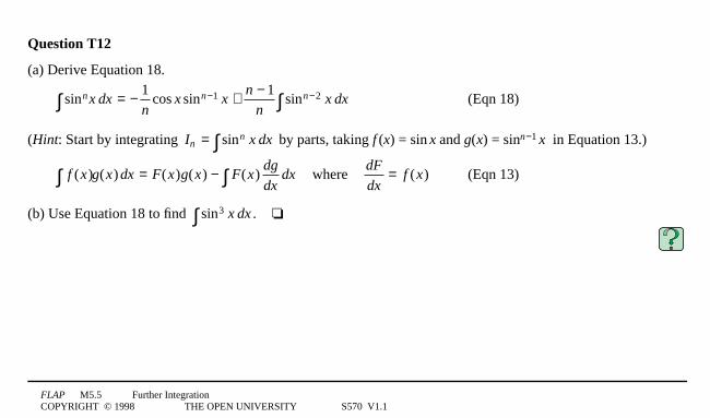
Question T12

(a) Derive Equation 18.

sinn∫ x dx = − 1n


sinn−2 x dx∫ (Eqn 18)

(Hint: Start by integrating In = sinn x dx∫ by parts, taking f1(x) = sin1x and g(x) = sinn−11x in Equation 13.)


dxdx4where4 dF

dx= f (x) (Eqn 13)

(b) Use Equation 18 to find sin3 x dx∫ .4❏


A third useful reduction formula deals with integrals of the form xn e−ax dx∫ where a is a positive constant and

n is a positive integer. Again we use integration by parts to derive the reduction formula. In the integral, we take

f1(x ) = e−a x and g (x) = xn, then F(x) = − 1a

e−ax and dg

dx= nxn−1 and substituting these expressions into

Equation 13,


dxdx4where4 dF

dx= f (x) (Eqn 13)

we obtain

e−ax

f ( x ){

xn

g( x ){∫ dx = − 1

ae−ax

F( x )1 24 34

xn( )g( x ){

− nxn−1

dg dx124 34

⌠

⌡

− 1a

e−ax

F( x )1 24 34

dx

so that xne−ax∫ dx = −xn 1a

e−ax + n

axn−1e−ax∫ dx (19) ☞

Equation 19 shows that we can express xn e−ax dx∫ in terms of xn−1 e−ax dx∫ , an integral involving one less

power of x.


In the simplest case, if n = 1 in Equation 19,

xne−ax∫ dx = −xn 1a

e−ax + n

axn−1e−ax∫ dx (Eqn 19)

we can find x e−ax∫ dx , and so obtain

x e−ax∫ dx = − x

ae−ax + 1

ae−ax∫ dx = − x

ae−ax − 1

a2e−ax + C

✦

Given that x e−ax∫ dx = − x

ae−ax − 1

a2 e−ax + C , find x2 e−ax dx∫ .


2.7 Mixed examples

Aside You may be aware of the existence of algebraic computing programs such as: Mathematica, Reduce, Maple, Mathcador Derive, which can find indefinite integrals, and evaluate definite integrals as functions of the parameters appearing inthem. If so, you may be wondering why you should bother to learn advanced integration techniques; why not just key in theintegral and let the program do the work? Such programs have their limitations. They may not give you the answer in theform you are expecting, for instance, in Example 6 we found

1

4 + 9x2

⌠⌡

dx = 1

3arcsinh

3x

2

+ C

but using Derive you would obtain

1

4 + 9x2

⌠⌡

dx = 1

3loge (9x2 + 4) + 3x + C .

It is not immediately obvious that these two answers are the same.

In the case of improper but convergent integrals, the program may decide (incorrectly) that the integral cannot be evaluated,and you may have to make a substitution in order to make the integral acceptable to the program. Such programs can be veryuseful, and they certainly alleviate the tedious business of calculating unpleasant integrals, but you would be very unwise touse them without understanding the basic principles of integration.


How to tackle a general integral

You have learnt several tricks that will enable you to find a wide variety of integrals. We do not intend tosummarize them here. First, their uses are so widespread that such a summary would be lengthy and boring;second (and more important) we do not want you to feel that you must learn by heart a long list of differenttypes of integral and the methods that will work for them. Certainly you should have these methods as part ofyour ‘mathematical furniture’, but you should think of them as techniques to be applied in a ‘trial and error’way. It is not a disaster if the first method you try does not work; you simply have to try something else.You should bear in mind too, that many integrals can only be found by a combination of the techniques you havelearnt here; it may, for example, be necessary for you to use more than one substitution, and perhaps combinesubstitutions with algebraic manipulation or use of identities. As you gain more experience with integration, youwill begin to see automatically what sort of approaches are likely to prove productive with a given integral.

The following two questions should serve as revision of the integration techniques we have discussed.


Question T13

Find the following integrals: ☞

(a) 1

x2 − 2x⌠⌡

dx (Hint: Use partial fractions.)

(b) cos7 (2x)sin4 (2x) dx∫ (Hint: Use trigonometric identities.)

(c) 1 − 4x

1 + 4x + 2x2⌠⌡

dx (Hint: Split the numerator; complete the square in the denominator; use a hyperbolic

function substitution.)

(d) (x2 − 1)3 2

1

2

∫ dx (Hint: Substitute a hyperbolic function; use the answer to Question T11.)4❏


Question T14

Find the following integrals:

(a) 3x + 2

(x2 + 2x + 2)(x − 1)⌠⌡

dx ,4(b) sin6 x dx0

π / 2

∫ ,4(c) x2

x2 − 4⌠⌡

dx .4❏


3 Some definite integrals

3.1 Integrals with an infinite upper or lower limitDefinite integrals in which one or both of the limits is infinite occur very often in physics. Here are someexamples:

V = Q

4πε0 x2dx

r

∞

∫ (20) ☞

1(x − x0 )2 + a2

dx−∞

∞

∫ , where x0 and a are constants, and a > 0 (21) ☞

⟨ v ⟩ = 4π m

2πkT

3/ 2

v3exp (−mv2 2kT )0

∞

∫ dv (22) ☞

xn e−ax

0

∞

∫ dx , where n is a non-negative integer, and a > 0 (23) ☞


Definite integrals over an infinite range of integration are known as improper integrals. The way to evaluatethem is to replace the infinite limit by a very large (but finite) number, evaluate the integral in the usual way, andthen see what happens to your result as the large number becomes larger still. More formally, we think of animproper integral as a limit:

f (x) dx = limb→∞

a

∞

∫ fa

b

∫ (x) dx

and f (x) dx = lima→−∞−∞

b

∫ fa

b

∫ (x) dx ☞

If you can find the indefinite integral F(x) + C = f (x) dx∫ , evaluating an improper definite integral of the form

f (x) dxa

∞

∫ simply requires you to know how the function F(x) behaves when x becomes very large. Often this is

obvious.


For example, to evaluate the integral in Equation 20,

V = Q

4πε0 x2dx

r

∞

∫ (Eqn 20)

we think of it as the limit as R → ∞ of

Q

4πε0 x2

r

R

⌠⌡

dx = − Q

4πε0 x

r

R

= − Q

4πε0 R+ Q

4πε0r

As R becomes very large, 1/R becomes smaller and smaller, so that as R → ∞ the first term tends to zero.So we are left with

V = Q

4πε0 x2

r

∞⌠⌡

dx = Q

4πε0r


Sometimes it may not be immediately obvious what happens to F(x) as x becomes very large.For example, at the start of Subsection 2.1 we showed that

1(x + 1)(x + 2)

⌠⌡

dx = loge (x + 1) − loge (x + 2) + C

Suppose that we want to find the definite integral 1

(x + 1)(x + 2)0

∞⌠⌡

dx . ☞ We can express this integral as

lima→∞

loge (x + 1) − loge (x + 2)[ ]0a ; what happens to the difference between two logarithms when their arguments,

i.e. (x +1) and (x + 2) both become very large? We can see what happens if we write this difference oflogarithms as the logarithm of a fraction:

loge (x + 1) − loge (x + 2) = logex + 1x + 2

As x becomes very large, the fraction tends towards the value 1, and its logarithm tends to zero.

So1

(x + 1)(x + 2)0

∞⌠⌡

dx = 0 − loge12

= 0.6931


✦

What is the limit as x → ∞ of 3x2 + 2x + 52x2 − 4x − 1

?

Another potentially tricky situation arises when we consider the integral in Equation 23, namely xn e−ax dx0

∞

∫ .

We are already part of the way in evaluating the indefinite integral xn e−ax dx∫ ; we derived a reduction formula

for it in Subsection 2.6:


e−ax + n


We can easily convert Equation 19 into a reduction formula involving definite integrals between 0 and ∞, byputting in the limits:

xn e−ax dx0

∞

∫ = − 1a

xn e−ax[ ]0

∞ + n

axn−1 e−ax

0

∞

∫ dx (24)


We now need to know what happens to the function xn 1e−ax as x becomes very large. There is something of adilemma here: e−ax becomes very small for large x (remember that a is positive), but xn becomes very large;which one wins? Although we will not prove it here, the rule is as follows:

xn1e−ax → 0 as x → ∞ (25) ☞

for any n and any positive constant a

Using this rule to evaluate the term xn e−ax[ ]0

∞ in Equation 24,

xn e−ax dx0

∞

∫ = − 1a

xn e−ax[ ]0

∞ + n

axn−1 e−ax

0

∞

∫ dx (Eqn 24)

we see that the function is zero at the upper limit; it is also zero at the lower limit (because of the factor xn).So Equation 24 becomes

xn e−ax dx0

∞

∫ = n

axn−1 e−ax

0

∞

∫ dx (26)


✦

Evaluate the integral e−ax dx0

∞

∫

✦

Evaluate the integrals x e−ax dx0

∞

∫ and x2 e−ax dx0

∞

∫ , using Equation 26.

xn e−ax dx0

∞

∫ = n

axn−1 e−ax

0

∞

∫ dx (Eqn 26)


You may be able to see a pattern emerging. If we now use Equation 26

xn e−ax dx0

∞

∫ = n

axn−1 e−ax

0

∞

∫ dx (Eqn 26)

to work out x3 e−ax dx0

∞

∫ , we find

x3 e−ax dx0

∞

∫ = 3 × 2 × 1a4

, x4 e−ax

0

∞

∫ dx = 4 × 3 × 2 × 1a5

4and so on.

The general result is

xn e−ax dx0

∞

∫ = n!an+1

(27) ☞

✦

Evaluate the integral x7 e−2 x dx0

∞

∫ .


So far, we have considered improper integrals which could be evaluated without using a substitution. Of course,if you want to evaluate an improper integral using a substitution, you will need to transform the infinite limit ofintegration appropriately. Sometimes it will turn into a finite quantity, as in the next example.

Example 10

Evaluate the integral 1

(x − x0 )2 + a2dx

−∞

∞⌠⌡

appearing in Equation 21.

Solution4This integral can be found using the substitution x − x0 = a1tan1u. Then dx = a1sec21u1du, and(x − x0)2 + a2 = a21sec21u. When x is very large and positive, so is x − x0 = a1tan1u. ☞ If a1tan1u is very large, then u is close to π/2, and as tan1u tends to infinity, u tends to π/2; so the upper limit ofintegration becomes π/2. Similarly, the lower limit of integration becomes −π/2. Thus

1(x − x0 )2 + a2

dx

−∞

∞⌠⌡

= 1a

1du = πa−π / 2

π / 2

∫ 4❏


It is usually quite straightforward to change infinite limits of integration on making a substitution of the formu = g(x) or x = h(u); you need only ask yourself ‘What does u tend to as x gets very large?’ Of course, often youwill find that the infinite limit of integration is still infinite. This is the case in the following question.

Question T15

Using the substitution u = v2, and Equation 27,

xn e−ax dx0

∞

∫ = n!an+1

(Eqn 27)

evaluate the integral

v3 exp (−mv2 2kT ) dvo

∞

∫ that appears in Equation 22.4❏ ☞


3.2 Gaussian integrals

Integrals of the form xr exp(−ax2 ) dx0

∞

∫ , where r is a positive integer or zero, and a is a positive constant, are

particularly common in physics. You have already seen one example of this sort in Equation 22

⟨ v ⟩ = 4π m

2πkT

3/ 2

v3exp (−mv2 2kT )0

∞

∫ dv (Eqn 22)

(and evaluated it in Question T15). Many others like this arise in the kinetic theory of gases, in quantummechanics, and also in probability theory (which you may find yourself using to analyse experimental data).

In the case where r is an odd integer, such integrals can easily be evaluated, using the same substitution that youemployed in Question T15. To make it clear that r is odd, we will write r = 2n + 1, where n is any positive

integer or zero, and consider the integral x2n+1

0

∞

∫ exp(−ax2 ) dx which we write as x2n exp(−ax2 )x dx0

∞

∫ .


We now make the substitution y = x2. Then x dx = 12

dy , and x2n = (x2)n = yn. So

x2n+1 exp (−ax2 ) dx0

∞

∫ = 12

yn e−ay dy0

∞

∫

We know how to evaluate yn e−ay dy0

∞

∫ ; from Equation 27,

xn e−ax dx0

∞

∫ = n!an+1

(Eqn 27)

it is equal to n!

an+1. Thus


∞

∫ = n!2an+1

(28)


✦

Evaluate x5

0

∞

∫ exp(−3x2 ) dx .

Notice, too, that because we can relate x2n+1 exp (−ax2 ) dx∫ to yn e−ay dy∫ by the substitution y = x 02, and we

can find the latter integral (for any given value of n) by applying Equation 19


e−ax + n


as many times as is necessary, there is no problem in finding the indefinite integral x2n+1∫ exp(−ax2 ) dx , should

we want to do so.


The situation is very different for the indefinite integral xr exp(−ax2 ) dx∫ where r is an even integer. If you try

the substitution x2 = y, you will quickly find that it does not help at all1 1there is an awkward factor of y left

over in the integrand. In fact, such indefinite integrals cannot be evaluated in terms of familiar functions (such as

exp, loge, powers of x and so forth). The simplest of these integrals (with r = 0, a = 1) is exp(−x2 )∫ dx .

This integral is in fact used to define a new function of x, known as the error function, erf(x); the precisedefinition is

erf (x) = 2π

exp(−y2 2)0

x

∫ dy

It is possible to evaluate this integral for different values of x by numerical techniques, and the results have beentabulated and can be looked up in books (indeed, some calculators have an ‘erf’ button). If you study advancedprobability theory in future, you are bound to come across this function. However, here we will be concerned

just with the definite integral exp(−x2 )0

∞

∫ dx , and definite integrals such as xr exp(−ax2 )0

∞

∫ dx (where r is an

even integer) which can be related to it. Such integrals are called Gaussian integrals.


It is possible to evaluate exp(−x2 )0

∞

∫ dx exactly by methods that are more advanced than those discussed in

FLAP; we will present the answer here, and then show that a whole host of other Gaussian integrals can befound in terms of this integral. The basic result is

exp(−x2 )0

∞

∫ dx = 12

π (29)

We can use Equation 29 to find the integral exp(−ax2 )0

∞

∫ dx . We simply make the substitution y = a x .

Then dx = 1a

dy , and the limits of integration are still 0 and ∞. So exp(−ax2 ) dx0

∞

∫ = 1a

exp(−y2 ) dy0

∞

∫ ,

and from Equation 29,

exp(−ax2 ) dx0

∞

∫ = 12

πa

(30)


✦

Evaluate exp(−ax2 ) dx−∞

∞

∫ .

We can now use integration by parts to derive a reduction formula relating xr exp(−ax2 ) dx0

∞

∫ to

xr −2 exp (−ax2 ) dx0

∞

∫ . To make it clear that r is an even integer, we write r = 2n, where n is any positive integer.

We can write the integral x2n exp(−ax2 ) dx0

∞

∫ as x exp(−ax2 )0

∞

∫ x2n−1 dx , and apply Equation 13,


dxdx4where4 dF

dx= f (x) (Eqn 13)

taking f (x) = x exp(−ax2 )4and4g(x) = x2n−1


Then F(x) = − 12a

exp(−ax2 ) (as you can easily check by differentiating), and dg

dx= (2n − 1)x2n−2 .

So x2n

0

∞

∫ exp(−ax2 ) dx = − 12a

x2n−1 exp (−ax2 )

0

∞

+ 2n − 12a

x2n−2

0

∞

∫ exp(−ax2 ) dx (32)

Now from the rule in Equation 25,

xn1e−ax → 0 as x → ∞ (Eqn 25)

(for any n and any positive constant a), we know that x 02n0−011e−ax tends to zero as x tends to infinity; and sinceexp1(−ax2) is smaller than e−ax when x is large, we can be sure that x02n0−011exp1(−ax2) also tends to zero as x tendsto infinity.

Since n ≥ 1, x 02n0−011exp1(−ax2) = 0 when x = 0. So the first term on the right-hand side of Equation 32 is zero,leaving us with the reduction formula

x2n

0

∞

∫ exp(−ax2 ) dx = 2n − 12a

x2n−2

0

∞

∫ exp(−ax2 ) dx (33)


We can now use this reduction formula,

x2n

0

∞

∫ exp(−ax2 ) dx = 2n − 12a

x2n−2

0

∞

∫ exp(−ax2 ) dx (Eqn 33)

and Equation 30,

exp(−ax2 ) dx0

∞

∫ = 12

πa

(Eqn 30)

to work out values of x2n

0

∞

∫ exp(−ax2 ) dx for successively higher values of n.

✦

Evaluate x2

0

∞

∫ exp(−ax2 ) dx .

Gaussian integrals may sometimes appear in a disguised form. In the following question you have to make asubstitution before it becomes clear that you are dealing with a Gaussian integral.


Question T16

Evaluate the integral x3/ 2

0

∞

∫ e−5x dx . (Start by making the substitution x = y2.)4❏

Finally, integrals of the form exp(−ax2 + bx)−∞

∞

∫ dx can be easily related to the integral appearing in

Equation 31, exp(−ax2 )−∞

∞

∫ dx ,

exp(−ax2 ) dx−∞

∞

∫ = 2 exp(−ax2 )0

∞

∫ dx = πa

(Eqn 31)

by the trick of completing the square in the exponent. The following example shows you how to proceed.


Example 11

Evaluate the integral exp(−2x2 + 4x)−∞

∞

∫ dx

Solution4We write −2x2 + 4x in completed square form:

−2x2 + 4x = −2(x02 − 2x) = −2[(x − 1)2 − 1] = −2(x − 1)2 + 2

Thus the integral can be written as exp[−2(x − 1)2 ]e2

−∞

∞

∫ dx . We now make the substitution y = x − 1, dy = dx.

The limits of integration are still −∞ and ∞; so, taking the constant e2 outside the integral sign, we have

exp[−2(x − 1)2 ]e2

−∞

∞

∫ dx = e2 exp (−2y2 ) dy−∞

∞

∫


Substituting a = 2 in Equation 31,

exp(−ax2 ) dx−∞

∞

∫ = 2 exp(−ax2 )0

∞

∫ dx = πa

(Eqn 31)

we find that exp(−2y2 ) dx =−∞

∞

∫π2

; so

exp(−2x2 + 4x) dx =−∞

∞

∫ e2 π2

≈ 9.2614❏

Question T17

Evaluate the integral exp(− 12 x2 − 3x)

−∞

∞

∫ dx4❏


3.3 Line integralsThis subsection discusses a type of definite integral that is known as a line integral. Line integrals can be used(among other applications) to evaluate the work done by a force, and we will introduce them in that context.

Suppose that an object moves along the x-axis under the influence of a constant force Fx in the x-direction.The work done by the force in moving the object from x = a to x = b is W = sxFx, where sx is the displacement ofthe object. If the force is not constant, but instead varies with x, Fx(x) say, then you may already know that the

work done in moving the object from x = a to x = b is given by the definite integral Fx (x)a

b

∫ dx .

To derive this result, we divide the interval a ≤ x ≤ b into many small subintervals: we introduce n + 1 values ofx such that a = x1 < x2 < … < xn < xn+1 = b, and we define ∆xi = xi0+1 − xi, where i is any integer in the range

1 ≤ i ≤ n and let |1∆x1| be the largest of these subintervals. We can then say that over any one of these smallintervals, the force is approximately constant, so that the work done by the force in moving the object from xi to

xi0+1 is approximately equal to Fx(xi)∆xi. Then the total work done by the force is approximately given by the sum

Fx (xi )i=1

n

∑ ∆xi (34)


As we increase the number n of subintervals, and let the size of each one become smaller and smaller,Equation 34

Fx (xi )i=1

n

∑ ∆xi (Eqn 34)

becomes a better and better approximation to the actual work done. In the limit as n tends to infinity and|1∆x1| tends to zero, we have

W = lim| ∆x |→0

Fx (xi )i=1

n

∑ ∆xi = Fxa

b

∫ (x) dx (35)


x

y

F

s

Figure 14A constant force F movingan object along a straight line.

Let us now generalize these ideas to the case where the object is notconstrained to move along the x-axis, but can move along a path in the(x, y ) plane, and where the force is not in the same direction as thedisplacement of the object. First, we need to know the work done if aconstant force F acts on the object so as to move it along a line that is notnecessarily parallel to F, as in Figure 1. You may know that the workdone is given by the scalar product of F and the displacement s of theobject:

W = F1·1s (36) ☞

If we resolve both F and s into their components along the x and y axes,so that

F = (Fx0, Fy)4and4s = (sx0, sy)

we have the alternative expression for W

W = Fx1sx + Fy1sy (37)


✦ A force of 201N acting in the y-direction moves an object along a straight line. The initial position of theobject is x = 21m, y = 31m, and its final position is x = 41m, y = 61m. What is the work done by the force?

Now consider the general case, where the object is constrained to move along a given curved path, and wherethe components of F may be functions of x and y. To show that the components of F are functions of x and y, wewill write the vector F as

F(r) = (Fx(x, y), Fy(x, y))

To derive an expression for W, we proceed much as we did in deriving Equation 35.

W = lim| ∆x |→0

Fx (xi )i=1

n

∑ ∆xi = Fxa

b

∫ (x) dx (Eqn 35)

Essentially the procedure is to divide the curved path into a large number of straight sections, find the work donemoving along each of these sections, then add together all these small contributions to find an estimate for thetotal work done.


x

y

ri

force

ra

rb

ri + 1

∆ri

F(r)

Figure 24An object moving under theaction of a variable force F(r).

We define an arbitrary position of the object by the vector r = (x, y),then suppose the initial position vector of the object is ra, and its finalposition vector is rb (see Figure 2). We divide the path of the objectinto n small subintervals. The position vector of the object at the start ofthe ith subinterval is ri-10, and at the end of it, the position vector is ri,where r0 = ra and rn = rb. We define ∆ri = ri0+1 − r i, and denote thecomponents of ∆ri by ∆xi and ∆yi, so that ∆ri = (∆xi0, ∆yi). We then let|1∆r1| denote the size of the largest subinterval ∆ri. As before, over anyone of these small intervals, the force is approximately constant, so wemay use either Equation 36

W = F1·1s (Eqn 36)

or Equation 37

W = Fx1sx + Fy1sy (Eqn 37)

to derive an approximate expression for the work Wi done by the force in moving the object from ri to ri0+1:

Wi = F(ri)1·1∆ri (38)


Wi = F(ri)1·1∆ri (38)

which can be rewritten in the form

Wi = Fx(x0i0, y0i)1∆xi + Fy(xi0, yi)1∆yi (39)

The total work done in moving the object from ra to rb is given, to a good approximation, by the sum of all theWi. As we allow the size of the largest subinterval, |1∆r1|, to tend to zero (so that n tends to infinity), theapproximation becomes more and more accurate, while the sums become integrals. We have two ways ofwriting the integral that results; using Equation 38, we have

W = lim

| ∆r |→0F(ri )

i=1

n

∑ ⋅∆ri = Fra

rb

∫ (r)⋅dr (40)

while using Equation 39 gives us

W = lim

| ∆r |→0Fx (xi , yi ) ∆xi + Fy (xi , yi ) ∆yi[ ]

i=1

n

∑

= Fx (x, y) dx + Fy (x, y) dy[ ]

ra

rb

∫ (41)

Equation 40 gives a very concise way of writing down the integral that determines W; but, as you will see, inpractice we use Equation 41 to evaluate the integral.


An integral of the form

F(r)⋅dr = Fx (x, y) dx + Fy (x, y) dy[ ]

ra

rb

∫ra

rb

∫is known as a line integral.

Study comment Many students have difficulties coming to grips with line integrals, and the source of the problems is oftena matter of understanding. It is important to remember that a line integral is a limit of a sum1—1that is the definition, (and onthe face of it, this has little to do with inverting the process of differentiation). Evaluating a line integral is a separate issue; itis a matter of turning the integral into a form that we recognize, and which we can calculate.

The path along which the object moves is crucial. If we know that the object’s path is determined by an equationy = f1(x), then we can express both Fx and Fy as functions of x only; we can also express dy in Equation 41

W = lim


i=1

n

∑

= Fx (x, y) dx + Fy (x, y) dy[ ]

ra

rb

∫ (Eqn 41)

in terms of dx. This means that the line integral becomes an ordinary definite integral1—1something that we knowhow to evaluate. A particular example should make the point clear.


Example 12

A force F = 2yi + 2x1j ☞ moves an object from the point (0, 0) to the point (1, 1) along the path y = x?

What is the work done on the object by the force? What is the work done if the same force moves the objectalong the path y = x2?

Solution We use Equation 41,

W = lim


i=1

n

∑

= Fx (x, y) dx + Fy (x, y) dy[ ]

ra

rb

∫ (Eqn 41)

substituting Fx(x, y) = 2y and Fy(x, y) = 2x. This gives

(2y dx + 2x dy)

ra

rb

∫ , where ra = 0 and rb = i + j. ☞

We need to evaluate this integral along two different paths.

(a) Along the path y = x, we have dy = dx. So we substitute y = x and dy = dx into Equation 41

W = Fx (x, y) dx + Fy (x, y) dy[ ]

ra

rb

∫ = ( 2yFx ( x ,y){

dx + 2xFy ( x ,y){

dy)ra

rb

∫

= ( 2y

let y= x{

dx + 2x dylet dy=dx

{

)ra

rb

∫ = (2x dx + 2x dx)ra

rb

∫


On the right-hand side we now have a definite integral over x, and the limits of integration are the values of x atthe points r = ra and r = rb, namely 0 and 1.

Thus W = (2x0

1

∫ dx + 2x dx) = 4x dx = 2x2[ ]0

1

0

1

∫ = 2

(b) Along the path y = x2 we have dy = 2x 1dx, so in this case

W = Fx (x, y) dx + Fy (x, y) dy[ ]

ra

rb

∫ = ( 2yFx ( x ,y){

dx + 2xFy ( x ,y){

dy)ra

rb

∫

= ( 2y

let y= x2{

dx + 2x dylet dy=2 xdx

{

)ra

rb

∫ = (2x2 dx + 4x2 dx)ra

rb

∫

Again the expression on the right-hand side is just an ordinary integral, and once more the limits of integrationare 0 and 1. So

W = (2x2 dx + 4x2 dx0

1

∫ ) = 6x2

0

1

∫ dx = 2x3[ ]0

1 = 24❏ ☞


Question T18

Find the work done when a force F = 2xyi − 3y1j moves an object from the point (1, 2) to the point (2, 4) alongthe line y = 2x.4❏

We will finish with two comments.

First, although we have discussed line integrals only for paths that lie in the (x, y) plane, they can of course be

written down for paths in three dimensions. In that case,

F(r)

ra

rb

∫ ⋅dr can be written as

Fx (x, y, z) dx + Fy (x, y, z) dy + Fz (x, y, z) dz[ ]

ra

rb

∫


To specify the path, we would need to know both y and z as functions of x; this knowledge would allow us toturn the line integral into a definite integral over x, as we did in Example 12.

Second, for some choices of the force F(r), the line integral

F(r)

ra

rb

∫ ⋅dr is actually independent of the path

chosen to evaluate the integral; it depends only on the coordinates of the endpoints of the path. (This is true ofthe force in Example 12.) Forces of this sort are known as conservative forces. It is possible to specify necessaryand sufficient conditions that the components of the force F must satisfy if F is to be conservative.This is beyond the scope of FLAP, but you are certain to meet them if you carry your study of physics further.


4 Closing items

4.1 Module summary

1 Integrals of the form p(x)q(x)

⌠⌡

dx , where p(x) and q(x) are polynomials in x, may often be converted into

sums of simpler integrals by writing the integrand in terms of its partial fractions.

2 If the method of partial fractions is to be useful, the denominator q(x) must factorize, at least partially.If q(x) is a quadratic function of x which does not factorize, the technique of writing q(x) in completedsquare form and making a substitution of the form x = tan1u allows us to find the integral.

3 Completing the square in the denominator, and making a substitution of the form x = sin1u, allows us to find

integrals of the form 1

a + bx − cx2⌠⌡

dx , where c > 0.

4 By splitting the numerator, we can write integrals of the form px + q

a + bx − cx2⌠⌡

dx and (in the case where

the denominator does not factorize) px + q

ax2 + bx + c⌠⌡

dx as sums of two simpler integrals.


5 Two standard integrals, which can be found by substitution of the hyperbolic functions x = sinh1u andx = cosh1u, respectively, are

1

x2 + 1⌠⌡

dx = arcsinh x + C and 1

x2 − 1⌠⌡

dx = arccosh x + C , where C is a constant of integration.

Integrals of the form 1

a + bx2⌠⌡

dx and 1

bx2 − a⌠⌡

dx , where a, b are positive constants, can be found

by the substitution x = d1sinh1u or x = d1cosh1u, where d is a suitably chosen constant.

6 Substitutions of hyperbolic functions may also be used to find many other integrals involving square rootsof quadratic functions of x, especially when combined with the techniques of completing the square orsplitting the numerator.

7 Trigonometric identities may be used to find integrals of products of powers of cos1x and sin1x(and the analogous identities for hyperbolic functions can similarly be used to find integrals of products ofpowers of cosh1x and sinh1x).


8 Reduction formulae are equations that relate an integral involving a power of x or some function of x to anintegral of the same form but involving a lower power of x or the function of x. Two examples are

cosn∫ x dx = 1n


cosn−2∫ x dx

and sinn∫ x dx = − 1n


sinn−2∫ x dx

These are useful in finding integrals of high powers of cos1x and sin1x.

9 Definite integrals in which one or both of the limits of integration is infinite are known as improperintegrals. They are to be found by treating the infinite limit as a very large number and allowing it to tend toinfinity; formally, we have

f (x)a

∞

∫ dx = limb→∞

f (x)a

b

∫ dx 4and4 f (x)−∞

b

∫ dx = lima→−∞

f (x)a

b

∫ dx


10 Using the rule that xn1e−ax → 0 as x → ∞, for any n and any positive constant a, and a reduction formula for

the indefinite integral xn e−ax dx∫ , we can derive a general result

xn e−ax dx0

∞

∫ = n!an+1

(Eqn 27)

Definite integrals of the form x2n+1 exp (−ax2 ) dx0

∞

∫ can be simply related to xn e−ax dx0

∞

∫ , allowing us to

derive the general result


∞

∫ = n!2an+1

(Eqn 28)


11 Gaussian integrals are definite integrals of the form x2n

0

∞

∫ exp(−ax2 ) dx . They may all be evaluated in terms

of the basic Gaussian integral, exp(−x2 ) dx0

∞

∫ = 12

π , using the reduction formula

x2n

0

∞

∫ exp(−ax2 ) dx =2n − 1

2ax2n−2

0

∞

∫ exp(−ax2 ) dx (Eqn 33)

12 A line integral of the form

F(r)

ra

rb

∫ ⋅dr is defined as a limit of a sum along a particular path. It may be

evaluated by using the equation of the path to convert the line integral into an ordinary definite integral.


4.2 AchievementsHaving completed this module, you should be able to:

A1 Define the terms that are emboldened and flagged in the margins of the module.

A2 Use algebraic techniques such as partial fractions, completing the square in the denominator, or splitting the

numerator to find integrals of the form p(x)q(x)

dx⌠⌡

, where p(x) and q(x) are polynomials in x.

A3 Find integrals which involve square roots of quadratic functions of x using the substitution of an appropriatehyperbolic function or trigonometric function.

A4 Use either trigonometric identities or reduction formulae to find integrals of products of powers of sin1x andcos1x (and use identities to find integrals of products of powers of sinh1x and cosh1x).

A5 Choose, for a given integral, a method or combination of methods that will enable you to evaluate it1 1andbe prepared to try another approach if your first one does not work.

A6 Evaluate definite integrals in which one or both of the limits is infinite.

A7 Use formulae such as xne−ax dx0

∞

∫ = n!an+1

and x2n+1 exp (−ax2 ) dx0

∞

∫ = n!2an+1

to evaluate definite integrals

of these types.


A8 Recognize Gaussian integrals, and integrals which can be related to these by means of a substitution or bycompleting the square in the exponent; and evaluate these using Equations 30 and 33.

A9 Evaluate a line integral along a specified path in the (x, y) plane.

Study comment You may now wish to take the Exit test for this module which tests these Achievements.If you prefer to study the module further before taking this test then return to the Module contents to review some of thetopics.


4.3 Exit test

Study comment Having completed this module, you should be able to answer the following questions, each of which testsone or more of the Achievements.

Question E1

(A2)4Find the integrals

(a) p

x2 (x − p)⌠⌡

dx , where p is a constant,4(b) 4x − 3

4x2 − 4x + 5⌠⌡

dx .

Question E2

(A3)4Find the integral 1

5 + 4x2⌠⌡

dx .


Question E3

(A4)4Find the integrals: (a) cos3(2x)sin4 (2x) dx∫ , (b) cos8 x dx0

π

∫ .

Question E4

(A5)4Find the integrals:

(a) x + 2

13 − 6x − 3x2⌠⌡

dx , (b) x cosh2 x dx∫ .


Question E5

( A 3 and A6)4By substituting an appropriate hyperbolic function, evaluate the definite integral

1(x2 + a2 )3/ 2

dx

0

∞⌠⌡

. (Hint: You may find the answers to Questions R6 and R7 useful here.)

Question E6

(A7, A8)4The Laplace transform ☞ of a function f1(x) is defined as the integral f (x) e−s x dx0

∞

∫ , where s > 0.

Find the Laplace transforms of the functions (a) x03,4(b) x .


Question E7

(A3 and A9)4A particle moves along the path y = x2 − 4 . It is acted upon by a force F = (−yi + x1j1)1N.

What is the work done by the force in moving the object from the point (2, 0) to the point (3, 5 )?

Study comment This is the final Exit test question. When you have completed the Exit test go back to Subsection 1.2 andtry the Fast track questions if you have not already done so.

If you have completed both the Fast track questions and the Exit test, then you have finished the module and may leave ithere.

flexible learning approach to physics ÊÊÊ module m5.5 further integration … › physics ›...

Documents