flight dynamics and control of highly flexible … dynamics and control of highly flexible...
TRANSCRIPT

Flight Dynamics and Control of Highly Flexible Flying-Wings
Brijesh Raghavan
Dissertation submitted to the Faculty of the
Virginia Polytechnic Institute and State University
in partial fulfillment of the requirements for the degree of
Doctor of Philosophy
in
Aerospace Engineering
Mayuresh J. Patil, Chair
Craig A. Woolsey
Rakesh K. Kapania
Leigh S. McCue
March 30, 2009
Blacksburg, Virginia
Keywords: Flexible high aspect-ratio flying-wings, flight dynamics, flight control
Copyright 2009, Brijesh Raghavan

Flight Dynamics and Control of Highly Flexible Flying-Wings
Brijesh Raghavan
(ABSTRACT)
High aspect-ratio flying wing configurations designed for high altitude, long endurance
missions are characterized by high flexibility, leading to significant static aeroelastic de-
formation in flight, and coupling between aeroelasticity and flight dynamics. As a result
of this coupling, an integrated model of the aeroelasticity and flight dynamics has to be
used to accurately model the dynamics of the flexible flying wing. Such an integrated
model of the flight dynamics and the aeroelasticity developed by Patil and Hodges is
reviewed in this dissertation and is used for studying the unique flight dynamics of high
aspect-ratio flexible flying wings. It was found that a rigid body configuration that ac-
counted for the static aeroelastic deformation at trim captured the predominant flight
dynamic characteristics shown by the flexible flying wing. Moreover, this rigid body con-
figuration was found to predict the onset of dynamic instability in the flight dynamics
seen in the integrated model. Using the concept of the mean axis, a six degree-of-freedom
reduced order model of the flight dynamics is constructed that minimizes the coupling
between rigid body modes and structural dynamics while accounting for the nonlinear
static aeroelastic deformation of the flying wing. Multi-step nonlinear dynamic inversion
applied to this reduced order model is coupled with a nonlinear guidance law to design
a flight controller for path following. The controls computed by this flight controller are
used as inputs to a time-marching simulation of the integrated model of aeroelasticity and
flight dynamics. Simulation results presented in this dissertation show that the controller
is able to successfully follow both straight line and curved ground paths while maintaining
the desired altitude. The controller is also shown to be able to handle an abrupt change
in payload mass while path-following. Finally, the equations of motion of the integrated
model were non-dimensionalized to identify aeroelastic parameters for optimization and
design of high aspect-ratio flying wings.

Dedicated
to
my mother and the memory of my father
iii

Acknowledgments
I would like to thank my adviser, Prof. Mayuresh Patil, for all his help and guidance
over the last four years. To say that this dissertation would not be possible without him
is an understatement. He has encouraged me when I felt that my dissertation topic was
too multi-disciplinary for me to solve, and has set high standards for us to meet. He
has always kept an open door for his graduate students and has always found the time
to explain things repeatedly till I was capable of understanding them. He has been very
considerate during some very difficult personal situations that I have been through, and
has let me take time off to take care of things back home.
I would like to thank Prof. Craig Woolsey, Prof. Rakesh Kapania and Prof. Leigh
McCue for serving on my PhD committee. Their input and feedback over the last three
years has been invaluable in helping me frame my problem statement, and in ensuring that
the quality of my work meets the standards of a dissertation. I would like to thank Prof.
Michael Philen for serving as the examiner for my defense in Prof. Kapania’s absence.
I would like to thank Prof. Christopher Shearer of AFIT for flying in all the way from
Ohio for my defense. His PhD dissertation at the University of Michigan was the first one
that addressed flight control of HALE airplanes, which made his feedback all the more
valuable. I would also like to thank Prof. Woolsey and Chris Cotting for helping me
understand the basics of nonlinear dynamic inversion.
Over the last three and a half years, I have probably spent more time in my office
than I have in any other location in Blacksburg. This has taken its toll on the mental
iv

well-being of my labmates and other people on the floor. Over the years, Rana, Jason,
Will, Chris, Jeff, Johannes, Thomas, Avani, Pankaj, Karen, Wes and Sameer have helped
me maintain my sanity in the face of seemingly unsurmountable MATLAB error codes.
They have put up with my pathetic sense of humor, loud and obnoxious laughter and
have helped me see the world from the perspective of different cultures (American and
European). I leave Femoyer 209 with pleasant memories, and I leave them all with some
of my bad habits to remember me by.
I met Lisa and Kenneth Granlund, Hamid Khameneh and Riley on my first hike to
McAfee’s Knob in the fall of 2005. Over the next two years, I spent many weekends
with them hiking the hills around Blacksburg and talking about things outside of work.
I would like to thank them for those wonderful trips, and I hope that they do visit me in
India someday ! I would like to thank my roommates over the years and my friends in
Blacksburg for some of the better days that I have spent here. One of my friends, Minal
Panchal, was murdered in the shooting in Norris Hall on April 16th 2007. In the brief
time that I knew her, she has left me with memories full of laughter and for that I will
always be grateful.
My stay here would not have been possible without my extended family back home.
In particular, I owe much to my relatives Elema and Balappapan and our neighbours
in Bombay, Daisy aunty and Joy uncle. They, along with other friends and family in
Bombay, were the people who talked to my father’s doctors and looked after him during
his final years, all duties that were mine to bear. I would like to thank my friends, Girish,
Shivangi, Gaurang, Kunal, Nag, Subbu, Praveena, Bharati, Payal, Girisha and Rana for
helping me out through some very difficult days.
My father passed away on 4th May 2006, less than nine months after I started graduate
studies here, and a week before I was due to arrive in India to see him. My mother has
been through exceptionally trying times over the last few years, but not once have I heard
her complain about the situations that she has had to face. My success has been built on
v

their sacrifices. Both my father and my maternal grandfather had to drop out of school
after 10th grade due to adverse financial circumstances. In many ways, this PhD meant
much more to them than it ever will for me. I hope that I have been able to give them
some measure of happiness from my academic success.
Last but not the least, I would like to thank the Aerospace and Ocean Engineering
Department for funding me for the first three years and for the Pratt Fellowship in 2009
and DARPA/Aero Institute for funding the final two semesters of my graduate studies.
vi

Contents
1 Introduction 1
1.1 Motivation . . . . . . . . . . . . . . . . . . . . . . . . . . . . . . . . . . . . 1
1.2 Objectives . . . . . . . . . . . . . . . . . . . . . . . . . . . . . . . . . . . . 2
2 Literature Survey 5
2.1 Flight Dynamics of Flexible Airplanes . . . . . . . . . . . . . . . . . . . . . 5
2.2 Flight Control of Flexible Airplanes . . . . . . . . . . . . . . . . . . . . . . 10
2.3 Aeroelasticity of High Aspect-Ratio Wings . . . . . . . . . . . . . . . . . . 13
2.4 Flight Dynamics and Control for Flexible High-Aspect Ratio Configurations 17
3 Integrated Model of Aeroelasticity and Flight Dynamics 23
3.1 Overview . . . . . . . . . . . . . . . . . . . . . . . . . . . . . . . . . . . . . 23
3.2 Structural Model . . . . . . . . . . . . . . . . . . . . . . . . . . . . . . . . 25
3.2.1 Geometrically-Exact Beam Equations . . . . . . . . . . . . . . . . . 25
3.2.2 Gravitational Model . . . . . . . . . . . . . . . . . . . . . . . . . . 34
3.2.3 Propulsive Model, nodal masses, and slope discontinuities . . . . . . 35
vii

3.3 Aerodynamic Model . . . . . . . . . . . . . . . . . . . . . . . . . . . . . . 36
3.4 Aeroelastic Equations . . . . . . . . . . . . . . . . . . . . . . . . . . . . . . 38
3.5 Open-loop Trim Computation and Linear Stability Analysis . . . . . . . . 38
3.6 Non-dimensional form and aeroelastic parameters . . . . . . . . . . . . . . 39
4 Control System Design 41
4.1 Overview . . . . . . . . . . . . . . . . . . . . . . . . . . . . . . . . . . . . . 41
4.2 Mean Axis Model . . . . . . . . . . . . . . . . . . . . . . . . . . . . . . . . 42
4.2.1 Equations of Motion . . . . . . . . . . . . . . . . . . . . . . . . . . 42
4.2.2 Application to current problem . . . . . . . . . . . . . . . . . . . . 47
4.2.3 Kinematic Equations . . . . . . . . . . . . . . . . . . . . . . . . . . 49
4.3 Control System Design . . . . . . . . . . . . . . . . . . . . . . . . . . . . . 50
4.3.1 Guidance Algorithm . . . . . . . . . . . . . . . . . . . . . . . . . . 50
4.3.2 Review of Dynamic Inversion . . . . . . . . . . . . . . . . . . . . . 51
4.3.3 Control Architecture for Flying Wings . . . . . . . . . . . . . . . . 53
4.4 Time-marching Implementation . . . . . . . . . . . . . . . . . . . . . . . . 56
4.5 Overview of Closed-Loop Simulation . . . . . . . . . . . . . . . . . . . . . 58
4.6 State Estimation for Control . . . . . . . . . . . . . . . . . . . . . . . . . . 59
5 Results 60
5.1 Open Loop Verification . . . . . . . . . . . . . . . . . . . . . . . . . . . . . 60
5.2 Open Loop Dynamics . . . . . . . . . . . . . . . . . . . . . . . . . . . . . . 62
viii

5.2.1 Sample configuration . . . . . . . . . . . . . . . . . . . . . . . . . . 63
5.2.2 Trim Computation . . . . . . . . . . . . . . . . . . . . . . . . . . . 64
5.2.3 Linear Stability Analysis for Straight and Level Trim . . . . . . . . 68
5.2.4 Stability Boundary for Straight and Level Trim . . . . . . . . . . . 71
5.2.5 Modified Static Stability Criteria . . . . . . . . . . . . . . . . . . . 71
5.3 Closed Loop Dynamics . . . . . . . . . . . . . . . . . . . . . . . . . . . . . 72
5.3.1 Path-following for straight line path . . . . . . . . . . . . . . . . . . 76
5.3.2 Path-following for curved ground path . . . . . . . . . . . . . . . . 84
5.3.3 Extreme cases . . . . . . . . . . . . . . . . . . . . . . . . . . . . . . 97
5.3.4 Path-following with abrupt change in payload mass . . . . . . . . . 116
5.3.5 Dependence of computational time on discretization . . . . . . . . . 119
6 Conclusions and Future Work 121
6.1 Conclusions . . . . . . . . . . . . . . . . . . . . . . . . . . . . . . . . . . . 121
6.2 Future Work . . . . . . . . . . . . . . . . . . . . . . . . . . . . . . . . . . . 122
Bibliography 124
ix

List of Figures
1.1 Methodology Followed . . . . . . . . . . . . . . . . . . . . . . . . . . . . . 2
3.1 Differential Thrust . . . . . . . . . . . . . . . . . . . . . . . . . . . . . . . 25
3.2 Beam Axis system . . . . . . . . . . . . . . . . . . . . . . . . . . . . . . . 26
4.1 Axis system . . . . . . . . . . . . . . . . . . . . . . . . . . . . . . . . . . . 42
4.2 Guidance Algorithm . . . . . . . . . . . . . . . . . . . . . . . . . . . . . . 50
4.3 Schematic of Control System . . . . . . . . . . . . . . . . . . . . . . . . . . 54
4.4 Closed-Loop Schematic . . . . . . . . . . . . . . . . . . . . . . . . . . . . . 58
5.1 Test for geometric exactness . . . . . . . . . . . . . . . . . . . . . . . . . . 61
5.2 Error Convergence plot for bending frequencies . . . . . . . . . . . . . . . 62
5.3 Schematic of configuration . . . . . . . . . . . . . . . . . . . . . . . . . . . 63
5.4 Trim Thrust variation with nodal mass . . . . . . . . . . . . . . . . . . . . 65
5.5 Root angle-of-attack variation with nodal mass . . . . . . . . . . . . . . . . 65
5.6 Flap deflection variation with nodal mass . . . . . . . . . . . . . . . . . . . 66
5.7 Aileron deflection variation with nodal mass . . . . . . . . . . . . . . . . . 67
5.8 ∆ Thrust variation with nodal mass . . . . . . . . . . . . . . . . . . . . . . 67
x

5.9 Root locus plot for Phugoid . . . . . . . . . . . . . . . . . . . . . . . . . . 68
5.10 Root locus plot for Lateral-Directional modes . . . . . . . . . . . . . . . . 69
5.11 Root locus plot for Dutch roll mode . . . . . . . . . . . . . . . . . . . . . . 70
5.12 Stability Boundary . . . . . . . . . . . . . . . . . . . . . . . . . . . . . . . 71
5.13 Straight and level path with initial vertical offset . . . . . . . . . . . . . . 77
5.14 Straight and level path with initial vertical offset . . . . . . . . . . . . . . 78
5.15 Straight and level path with initial lateral offset . . . . . . . . . . . . . . . 80
5.16 Straight and level path with initial lateral offset . . . . . . . . . . . . . . . 81
5.17 Straight and level path with initial lateral offset . . . . . . . . . . . . . . . 82
5.18 Straight and level path with initial lateral offset . . . . . . . . . . . . . . . 83
5.19 Straight and level path with initial lateral offset . . . . . . . . . . . . . . . 84
5.20 Curved ground path with no initial offset . . . . . . . . . . . . . . . . . . . 86
5.21 Curved ground path with no initial offset . . . . . . . . . . . . . . . . . . . 87
5.22 Curved ground path with no initial offset . . . . . . . . . . . . . . . . . . . 88
5.23 Curved ground path with no initial offset . . . . . . . . . . . . . . . . . . . 89
5.24 Curved ground path with no initial offset . . . . . . . . . . . . . . . . . . . 90
5.25 Curved ground path with initial vertical and lateral offset . . . . . . . . . . 92
5.26 Curved ground path with initial vertical and lateral offset . . . . . . . . . . 93
5.27 Curved ground path with initial vertical and lateral offset . . . . . . . . . . 94
5.28 Curved ground path with initial vertical and lateral offset . . . . . . . . . . 95
5.29 Curved ground path with initial vertical and lateral offset . . . . . . . . . . 96
xi
5.30 Straight and level path with initial vertical offset (large offsets) . . . . . . . 98
5.31 Straight and level path with initial vertical offset (large offsets) . . . . . . . 99
5.32 Straight and level path with initial lateral offset (large offsets) . . . . . . . 101
5.33 Straight and level path with initial lateral offset (large offsets) . . . . . . . 102
5.34 Straight and level path with initial lateral offset (large offsets) . . . . . . . 103
5.35 Straight and level path with initial lateral offset (large offsets) . . . . . . . 104
5.36 Straight and level path with initial lateral offset (large offsets) . . . . . . . 105
5.37 Curved ground path with no initial offset (small radii) . . . . . . . . . . . 106
5.38 Curved ground path with no initial offset (small radii) . . . . . . . . . . . 107
5.39 Curved ground path with no initial offset (small radii) . . . . . . . . . . . 108
5.40 Curved ground path with no initial offset (small radii) . . . . . . . . . . . 109
5.41 Curved ground path with no initial offset (small radii) . . . . . . . . . . . 110
5.42 Curved ground path with no initial offset (guidance law activated early) . . 111
5.43 Curved ground path with no initial offset (guidance law activated early) . . 112
5.44 Curved ground path with no initial offset (guidance law activated early) . . 113
5.45 Curved ground path with no initial offset (guidance law activated early) . . 114
5.46 Curved ground path with no initial offset (guidance law activated early) . . 115
5.47 Path following with abrupt change in payload mass . . . . . . . . . . . . . 117
5.48 Path following with abrupt change in payload mass . . . . . . . . . . . . . 118
5.49 Path following with abrupt change in payload mass . . . . . . . . . . . . . 119
5.50 Variation of computational time with number of nodes . . . . . . . . . . . 120
xii

List of Tables
5.1 Geometric parameters for Goland Wing . . . . . . . . . . . . . . . . . . . . 60
5.2 Elastic parameters for Goland Wing . . . . . . . . . . . . . . . . . . . . . . 60
5.3 Verification results . . . . . . . . . . . . . . . . . . . . . . . . . . . . . . . 61
5.4 Geometric parameters for HALE configuration . . . . . . . . . . . . . . . . 63
5.5 Elastic parameters for HALE configuration . . . . . . . . . . . . . . . . . . 63
5.6 Longitudinal Eigenvalues . . . . . . . . . . . . . . . . . . . . . . . . . . . . 69
5.7 Lateral-Directional Eigenvalues . . . . . . . . . . . . . . . . . . . . . . . . 70
5.8 Static correction factor . . . . . . . . . . . . . . . . . . . . . . . . . . . . . 74
xiii

Nomenclature
A beam cross-sectional area
a computed acceleration
b wing span
C rotation matrix
Ca rotation matrix from aerodynamic frame to local beam frame
CD Coefficient of drag
CL Coefficient of lift
Cm Coefficient of moment
c local chord
dl structural element length
E Young’s Modulus
e1, e2, e3 unit vector along x,y and z axis respectively
F internal force
f external force
G Shear Modulus
g gravity vector
g0 magnitude of gravity vector
H angular momentum
h altitude
I moment of inertia
J torsion constant
xiv

k initial curvature of wing
k2,k3 Shear correction factor
K gain value
L reference length
l semi-span of wing
M internal moment
M Mass
m external moment
N total number of elements
P linear momentum
q dynamic pressure
R,S, T cross-sectional flexibility coefficient
ri turn rate in inertial frame
r,R position vector
T thrust value
u displacement of a point on the beam axis
V linear velocity
x, y, z elements of position vector in inertial frame
X state-vector
γ flight path angle
ψ, θ, φ yaw, pitch and roll angles respectively
χ yaw angle of velocity vector in inertial frame
I 3×3 identity matrix
δ control surface deflection
ε stain of beam axis under loading
κ curvature of beam axis under loading
µ mass of element
ξ center of mass offset
xv
Ω angular velocity
λ inflow vector
λ0 inflow coefficient
ρ density of air
Subscript
aero aerodynamic in nature
B local beam axis
c value commanded by dynamic inversion
cg center of gravity
g gravitational in nature
i inertial reference frame
l lateral, value to the left of node
M mean reference frame
mr root to mean transformation
mi inertial to mean transformation
T propulsive in nature
R root reference frame
ri inertial to root transformation
r value to the right of the node
∞ free-stream condition
Superscripts
B local beam axis in the deformed frame
b local beam axis in the undeformed frame
d demanded rate
n nth node/element
ng reference node for computing gravity vector components in beam axis
I inertial reference frame
M mean reference frame
xvi

R root reference frame
ˆ nodal value
mean value over the beam element
˜ cross product matrix
′ derivative along beam X co-ordinate
˙ derivative with respect to time
xvii
Chapter 1
Introduction
1.1 Motivation
High Altitude, Long Endurance (HALE) Unmanned Aerial Vehicles (UAVs) are designed
to cruise above 60,000 ft and fly missions ranging from a few days to a few years [1].
This unique flight profile makes it possible to use these aircraft as platforms for scien-
tific research, aerial photography and telecommunication relay. The demand for these
capabilities in both the civilian and the military sectors has been the motivation for the
development of HALE UAVs over the past two decades.
The Environmental Research Aircraft and Sensor Technology (ERAST) program was
conducted by NASA from 1994 to 2003 with the primary objective of developing HALE
UAVs [1]. As part of this program, Aerovironment developed a series of solar-powered
flying wing configurations, whose aspect-ratio increased progressively from 12 to 30.9
along with a corresponding increase in payload capability. The final airplane in this series,
Helios, encountered atmospheric turbulence and crashed during a flight test off the island
of Kauai, Hawaii on 26th June 2003 [2]. The atmospheric turbulence encountered during
the flight test caused the flying wing to deform to an unstable, high-dihedral configuration.
This in turn led to divergent pitch oscillations during which the airplane exceeded its
1

Chapter 1. Introduction
design airspeed and led to the failure of its wing panels. The mishap investigation report
concluded that the decision to test fly the crashed configuration was a flawed one, but
it has been made because available analysis tools were unable to predict the sensitivity
of the configuration to disturbances. The report further suggested the development of
“more advanced, multidisciplinary (structures, aeroelastic, aerodynamics, atmospheric,
materials, propulsion, controls, etc) ‘time-domain’ analysis methods appropriate to highly
flexible, ‘morphing’ vehicles”.
In 2007, DARPA initiated the Vulture program to develop technology for an air-
craft capable of uninterrupted flight for atleast five years [3]. Two of the three concepts
currently being studied involve high-aspect ratio wings [4, 5, 6].
1.2 Objectives
Figure 1.1: Methodology Followed
2

Chapter 1. Introduction
For conventional airplane configurations, the structural deformation under flight loads
(i.e. the static aeroelastic deformation) is not significant enough to influence the flight
dynamics and no significant interaction is observed between the rigid body modes and
aeroelastic modes. Therefore, the modeling for flight dynamics and aeroelastic analysis for
such configurations can be decoupled and can be carried out separately. Analysis of flight
dynamics is carried out by assuming a perfectly rigid structure based on the undeformed
shape as shown in sequence A in Fig. 1.1. These models are used as the basis for flight
control design. Aeroelastic analysis, on the other hand, is carried out on a flexible model
of the airplane structure with no rigid body degrees of freedom as shown in sequence B
in Fig. 1.1.
However, a low weight, high aspect-ratio wing design exhibits high flexibility and
undergoes significant deformation in flight. Moreover, the aeroelastic and flight dynamics
frequencies overlap and the flight dynamics and aeroelastic modes are coupled. The
influence of both static and dynamic aeroelastic effects on the flight dynamics becomes
significant, and has to be accounted for in the flight dynamics model. The analysis of
the flight dynamics and aeroelasticity has to be carried out in an integrated manner as
shown in the sequence C in Fig. 1.1. Such an integrated model was developed by Patil
and Hodges in 2003 [7] and has been reviewed in the third chapter of this dissertation.
Due to this coupling between aeroelasticity and flight dynamics, flight control de-
sign has to be carried out on an integrated model of the total dynamics of the system.
However, a reduced order model can be used for flight control design if the coupling be-
tween aeroelasticity and flight dynamics is minimized. This is accomplished by writing
the equations of motion in the mean axis system as shown in the fourth chapter. These
equations in the mean axis system capture the rigid body modes and static aeroelastic
deformation of the flying wing, and minimize the interaction between structural dynamics
and the rigid body modes.
In order to analyse the accuracy of this reduced order model, this dissertation studies
3

Chapter 1. Introduction
the unique flight dynamics of a flexible, high aspect-ratio flying-wing, with an emphasis on
the influence of static aeroelasticity on the flight dynamics. The dynamic characteristics of
the fully flexible configuration are compared with those of an equivalent rigid-body model
based on the deformed shape under static aeroelastic loading (henceforth referred to as
the statically deformed configuration). The flight dynamics of the statically deformed
configuration is analyzed as depicted in sequence D of Fig. 1.1. A modified criteria for the
onset of static flight dynamic instability in the presence of static aeroelastic deformation
is also presented.
The second objective is the design of a flight control system for path-following for
a flexible, high aspect-ratio flying wing. This is accomplished by a combination of a
nonlinear guidance law and a nonlinear dynamic inversion controller applied to a six
degree-of-freedom reduced-order model of the dynamics written in the mean axis system
as shown in the fourth chapter. The control inputs and the closed-loop response for the
flexible flying wing for path-following for a straight-line ground path and for a curved
ground path are presented. The controller is also shown to be able to handle an abrupt
change in payload mass while path-following.
Finally, the dissertation identifies non-dimensional aeroelastic parameters that can be
used for design and optimization of flexible, high aspect-ratio flying wings, and presents
expressions for estimating the state variables required by the controller from measured
flight data.
The work presented in this dissertation is directly applicable to unswept, high aspect-
ratio, highly flexible flying wings whose structure can be accurately modeled using non-
linear beam theory and whose aerodynamics is captured by two-dimensional, unsteady,
incompressible, potential flow models. The applicability of the flight dynamic analysis
and the flight control design presented here will have to be reviewed for a flying wing
which does not satisfy any of the assumptions mentioned above.
4

Chapter 2
Literature Survey
The literature review is divided into four sections. The first two sections review litera-
ture on flight dynamics and controls of generic flexible configurations. The third section
presents literature on the aeroelasticity of high aspect-ratio wings. The final section re-
views research specific to the flight dynamics and control of flexible, high aspect-ratio
configurations.
2.1 Flight Dynamics of Flexible Airplanes
In one of the earliest works on flight dynamics of flexible airplanes, Skoog studied the
effect of aeroelasticity on the longitudinal static stability of airplanes [8]. Flexibility was
found to change the spanwise aerodynamic loading distribution and shift the aerodynamic
center forward, leading to a reduction in longitudinal static stability. This effect was found
to be more pronounced at higher sweepback angles and aspect ratios. The lift-curve slope
of the wing was also reduced, leading to an increase in the angle of attack required for
trim. This in turn increased the stability contribution of a rigid horizontal tail, leading
to an effective increase in static stability. A conventional airplane configuration with a
5

Chapter 2. Literature Survey
swept wing was analyzed and it was found that torsional deflections had a stabilizing
effect while bending deflections had a destabilizing effect. However, the net effect of these
two factors was dependent on the ratio of bending to torsional rigidities, location of elastic
axis and the sweep angle. In a two part paper, Milne introduced the concept of the mean
axis, which decouples the equations of motion for flight dynamics from the equations for
structural dynamics for small deformations [9]. The paper developed the equations of
motion for a flexible airplane, and studied the equilibrium and stability of the airplane
for small perturbations. The concept of the mean axis, which is central to the control
design presented in this dissertation, was further elaborated upon in another paper by
the same author [10]. Wykes and Lawrence studied the effect of aerothermoelasticity
on the longitudinal stability and control of a supersonic transport configuration with a
canard and delta wings [11]. New stability derivatives were introduced to account for the
effect of flexibility on the flight dynamics of the airplane. Fuselage flexibility was found to
cause elevon reversal, and the coupling of the short period mode with the first symmetric
fuselage bending mode was seen to result in a dynamic instability.
Rodden’s analysis of experimental data showed that the the lateral stability derivative
for rolling moment with respect to sideslip (Clβ) changes significantly with a change
in dihedral angle under high load factors [12]. An analytical correction factor for the
stability derivative was introduced and a new method for predicting the correction in
terms of structural and aerodynamic influence coefficients was presented. Swaim and co-
workers modeled the longitudinal and lateral dynamics of elastic airplanes in a series of two
papers [13, 14]. Aerodynamic forces and moments induced by elastic modes were modeled
as functions of rigid-body stability derivatives, while neglecting flexibility corrections to
rigid-body stability derivatives themselves. Most of the terms in the new state space
model showed good agreement with experimental data for the B1 bomber. In a two-part
series Weisshaar and Ashley studied the static aeroelasticity of flying wing configurations
[15, 16]. Rigid body degrees of freedom were found to significantly alter the divergence
speed as compared to those for a cantilevered wing. An unswept flying wing trimmed in
6
Chapter 2. Literature Survey
roll using elevons was found to exhibit antisymmetric torsional divergence due to control
ineffectiveness [16]. The speed at which this instability occurs was found be dependent
on aerodynamic and geometric parameters of the wing [15]. The unswept flying wing
trimmed in level flight was found to exhibit symmetric divergence at twice the speed as a
cantilevered wing.
In their derivation of the equations of motion of flexible airplanes, Rodden and Love
modeled static aeroelastic deformation of the structure and numerically showed the error
in predictions when the correct axis system in not used for modeling the dynamics of the
airplane [17]. However, an error was found in the derivation of the equations of motion
presented in this paper and it was corrected in a paper by Dykman and Rodden [18]. It
was shown that the equations for dynamics of structural modes cannot be augmented to
the equations for the dynamics of statically deformed airplane without adding a correction
factor. This paper also compared the accuracy of a solution with truncated high frequency
dynamic modes, a solution with some dynamic modes residualized and a solution with all
dynamic modes residualized with the complete dynamic solution. The solution with all
dynamic modes residualized was found to have good accuracy except when the airplane is
subject to abrupt control inputs, as this excites the structural modes. The solution with
dynamic modes truncated without residualization was found to have limited accuracy.
In similar work, Karpel formulated a dynamic residual model for a flexible airplane that
accounted for aerodynamic effects dependent on the velocity of the modes [19]. For the
example considered in the paper, this formulation was found to substantially decrease
the error as compared to a model that uses modal truncation. The increase in computa-
tion time was found to be reasonable considering the improvement in accuracy and the
subsequent time savings obtained from reduced order models.
Waszak and Schmidt derived the equations of the motion for a flexible airplane in
the mean axis system using Lagrange’s equation and the principle of virtual work [20].
The derivation assumed small deformation, pre-computed modes of vibration, aerody-
namic strip theory and a constant inertia matrix. The equations for flight dynamics and
7

Chapter 2. Literature Survey
structural dynamics were coupled through the dependence of generalized forces on the
generalized displacement co-ordinates. Three configurations with varying degrees of flex-
ibility were numerically analyzed in the paper. The results showed that a model where
structural modes are residualized is more accurate as compared to a model where the
structural modes are truncated. However, even the residualized model showed significant
inaccuracies as compared to results from the full flexible model as the flexibility of the air-
plane increases. This modeling of equations of motion for a longitudinal airplane was later
reviewed in a paper by Schmidt and Raney [21], where visual-motion simulator studies
found that decreasing the lowest structural frequency has an adverse effect on the handling
quality of the airplane. Aeroelastic coupling was found to degrade ride quality and vibra-
tions felt at the cockpit influenced the precision of control inputs, resulting in involuntary
control inputs. The latter effect, known as biodynamic feedback, was especially pro-
nounced in the case of lateral vibrations of the airplane structure. Newman and Schmidt
presented three numerical techniques for model reduction [22]. These methods were ap-
plied to the model for longitudinal dynamics of a flexible airplane developed in Ref. [20].
Of the three numerical reduction techniques presented, the frequency-weighted balanced
technique was found to give superior results to both the residualization and truncation
techniques. A method for obtaining literal approximations was also presented that cap-
tures the pole-zero structure and numerical values of the coefficients of the reduced-order
models obtained using numerical model-reduction techniques. The procedure for obtain-
ing literal approximations was automated, and literal approximations were presented for
a subsonic flexible configuration, a supersonic missile and a hypersonic configuration in
a paper by Livneh and Schmidt [23]. The set of unified literal approximations presented
in the paper was found to be more accurate than approximations of longitudinal modes
obtained by decoupling the rigid body and aeroelastic modes.
Siepenkotter and Alles studied the nonlinear stability characteristics of a flexible air-
plane configuration by defining eigenvalues and eigenvectors as functions of perturbation
from the equilibrium point [24]. The integrated flexible aircraft model was based on
8

Chapter 2. Literature Survey
previous work [9, 20, 25], and three bending and one torsion mode were used to model
wing flexibility. Linear stability analysis carried out at straight and level trim showed the
spiral mode to be unstable. Nonlinear stability analysis presented in the paper detected
the presence of a stable equilibrium corresponding to a non-zero roll angle, which was
confirmed by an open-loop simulation. Drela modeled the dynamics of a flexible aircraft
using nonlinear beams for the structure and an unsteady lifting line model with compress-
ibility correction for the aerodynamics [26]. The trim point for the nonlinear system was
computed using a Newton-Raphson solver, and time marching was carried out using a
backward-difference formulation. The model was used to generate a root-locus plot for a
sailplane with flight speed as the parameter. Winther et al. derived reduced order equa-
tions for a flexible airplane by eliminating the auxiliary state variables required to model
unsteady aerodynamics [27]. The equations were transformed from the body axis to the
mean axis and equations for structural dynamics were integrated with the quasi-steady
nonlinear equations of motion.
Equations of motion for a flexible airplane configuration were rederived by Burtill et
al. while retaining inertial coupling terms between angular motion and flexibility [25].
A scalar parameter introduced in the paper can be used to determine if the coupling is
significant for the case considered. Reschke derived the nonlinear equations of motion for
flexible aircraft with a special focus on the inertial coupling between maneuvering flight
and structural dynamics of the airframe [28]. The force summation method, used for
calculation of aerodynamic and inertial loads acting on the airplane for a given trajectory,
was extended to account for inertial coupling. The residualized model approach used for
integrating the aerodynamic models with the equations of motion was extended to work
with the force summation method and quasi-flexible aerodynamic loads. The influence of
inertia coupling was found to be significant for high angular-rate/acceleration maneuvers.
Nguyen derived equations for the flight dynamics of a flexible airplane that accounts for
aeroelastic, propulsive and inertial coupling [29]. The structural dynamics of the wing
was modeled using an equivalent beam model and solved using finite element analysis to
9

Chapter 2. Literature Survey
obtain generalized co-ordinates corresponding to symmetric and anti-symmetric structural
modes. These generalized co-ordinates were used to couple the flight dynamic equations
with the structural dynamics of the wing though the force and moment expressions in the
flight dynamic equations.
2.2 Flight Control of Flexible Airplanes
Freymann studied the change in aircraft dynamic behavior resulting from the presence of
an active control system [30]. The paper presented examples of the four types of coupling
arising from the interaction of the control system designed for a flexible or rigid body
mode with another flexible or rigid body mode. In some cases, this coupling was found to
result in a decrease in the flutter speed or an instability in a rigid bode mode. Kubica et al.
introduced a new control synthesis technique for aircraft with significant coupling between
flight mechanics and structural dynamics modes [31]. By combining optimal control and
eigenstructure assignment through optimization, this technique can be used to stabilize
flight dynamic and structural modes and increase parameter robustness. Becker et al.
presented an integrated design of the flight control system and notch filters on the basis
of a coupled flight dynamic and structural dynamic model [32]. The new design was found
to reduce degradation in rigid body stability margins and improve elastic mode stability.
Etten et al. presented an integrated flight and structural modal control design for a flexible
aircraft using linear parameter varying methods, and compared it with another controller
in which the flight control and structural modal control were designed sequentially [33].
The handling and ride qualities of the closed loop systems were compared using µ analysis.
The integrated controller was found to be more robust to uncertainties in air density, and
also gave higher aeroelastic damping with lower control input.
Miyazawa extended the multiple-delay-model and multiple-design-point approach to
make it applicable to airplane configurations that show coupling of the control system
10

Chapter 2. Literature Survey
with the flexible structure [34]. A new criteria for structural-control coupling stabil-
ity was introduced. Alazard designed a robust lateral controller for a flexible airplane
configuration using H2 synthesis [35]. The control synthesis described in the paper is
a multi-step process that involves sequential tuning of gains. The paper also looked at
the robustness of the closed-loop system with respect to sensor location and selection.
Goman et al. compared an integrated flight and aeroelastic controller designed using µ
synthesis to a conventional controller designed using rigid body mode feedback and notch
and lag filters [36]. The step-response of both controllers were found to be quite similar
as the configuration presented in the paper does not exhibit coupling between the control
system and the structure. However, the closed-loop system with the integrated controller
exhibited more robustness than the one with the conventional controller. Silvestre and
Paglione derived the equations for dynamics of a flexible airplane in the mean axis system
using a modal superposition approach for the structural dynamics and a quasi-steady
aerodynamic model [37]. A controller was designed for disturbance rejection using the
H∞ static output-feedback approach.
Over a series of three papers, Gregory addressed the problem of applying a dynamic
inversion to control a large flexible aircraft [38, 39, 40]. The modified dynamic inversion
controller presented in the first paper was designed to follow control inputs while min-
imizing elastic deflections at the front end of the fuselage. The controller was designed
on a longitudinal model with eight elastic modes and applied on a longitudinal model
with twenty elastic modes. The dependence of longitudinal and elastic modal states on
actuator rates and accelerations was also modeled. These effects may not be insignifi-
cant for an elastic airplane due to unsteady aerodynamic and mass coupling effects. It
was found that the stability augmentation system and structural modal system had to
be designed in an integrated fashion, as the stand-alone stability augmentation system
used for comparison drove the fuselage structural modes unstable and drove one of the
control surfaces to its rate limit [38]. The next paper in the series dealt with the modifica-
tion introduced in the dynamic inversion control law to make it applicable to the flexible
11

Chapter 2. Literature Survey
configuration [39]. It was shown that the time constant of a first-order filter introduced
in the dynamic inversion loop changed the damping of a flexible mode in a stand-alone
second-order flexible model. This influence of the first-order filter on the damping of the
flexible mode was also found in the complete elastic model of the airplane. It was also
found that individual dynamics can be controlled by changing the corresponding filter
time constant while leaving the other filter time constants unchanged. The final paper
in the series presented stability results for the dynamic inversion controller as applied to
the flexible aircraft problem [40]. Results were presented for a simplified model. Only
one flexible mode was modeled along with longitudinal dynamics, and the control law was
designed only for flight control. The analysis considered only the dynamic inversion part
of the controller and the part specifying the desired dynamics was not analyzed.
Meirovitch and Tuzcu derived a unified formulation for dynamics of a flexible aircraft
using a Lagrangian approach [41]. The fuselage, wings and empennage structure were
modeled as beams undergoing bending and torsion, and aerodynamics was modeled using
two-dimensional strip theory. The equations were written in state-space form and sepa-
rated into a zero-order form for aircraft maneuvering and a first-order form consisting of
small perturbations in the rigid body states and elastic deformations. These perturbation
equations were used for control design using both the LQR and LQG approach for straight
and level flight and a steady, level turn. Stability was analyzed by computing eigenvalues
of both the closed and open loop system and simulations were presented by numerically
integrating the closed loop equations. Improved results were presented in a follow-up pa-
per which replaced component shape functions used for structural modeling with global
aircraft shape functions, and introduced new controller and observer designs [42]. These
global aircraft shape functions, which were derived by solving the eigenvalue problem of
a free-free aircraft at unstrained equilibrium in the absence of aerodynamic forces, allow
the structural deformation to be modeled with fewer states. The third paper in the series
studied the coupling between aeroelastic and flight dynamic modes for straight and level
flight and for a steady level turn [43]. The restrained airplane configuration with no rigid
12

Chapter 2. Literature Survey
body modes of freedom was found to be asymptotically stable. However in both cases, an
LQR controller that ensures closed-loop stability for the corresponding rigid body config-
uration was found to destabilize the flexible unrestrained airplane. This instability was
attributed to the coupling between rigid body and flexible modes. The final paper pre-
sented simulation results for a flexible airplane that flies a time-varying pitch maneuver
[44]. A new controller consisting of a combination of LQR and direct feedback controls
method was introduced and the controls are computed in discrete time. Point actuators
are used to suppress vibrations on the wind and empennage.
2.3 Aeroelasticity of High Aspect-Ratio Wings
Patil et al. studied the effects of geometric non-linearities arising from large deformation
on the aeroelasticity of high aspect-ratio wings [45]. Dynamic aeroelastic characteristics
were found to be significantly altered due to wing deformation and were found to be
dependent on the relative values of the structural frequencies. The deflection of the
wing under loading was found to result in a coupling between the bending and torsion
modes. The increase in deflection was also found to result in a significant decrease in
the flutter speed. The predominant cause of this decrease in flutter speed was shown
to be steady-state wing curvature under loading, which was also found to decrease the
effective lift generated by the wing in the vertical direction. It was found that this
effect could be canceled out by pre-curving the wing to give an effectively straight wing
under nominal flight loads. Similar results were obtained by Frulla who improved flutter
characteristics by increasing the bending stiffness [46]. A follow-up paper by Patil and
Hodges looked at the effects of aerodynamic and structural non-linearities on aeroelastic
behavior [47]. Aerodynamics was modeled using a non-planar fixed wake vortex lattice
method for the quasi-steady part and a doublet-lattice method for the unsteady part.
The effect of the nonplanarity on both steady and unsteady loads calculation was found
to be negligible, and three dimensional effects were found to be significant only at the
13

Chapter 2. Literature Survey
wing tip. However, the nonplanar shape of the wing was found to have a significant effect
on the local angle of attack at any wing section and the component of the airloads in the
vertical direction. Static structural deflection was captured accurately by linear structural
models, though the effect of the deflection on the dynamics was not modeled accurately by
linear models. A model that accounts for the steady state structural deformation and uses
a two-dimensional unsteady loads model, as opposed to a nonplanar three-dimensional
model, was found to accurately predict the aeroelastic behavior of the high aspect-ratio
wing.
Patil et al. developed a model for studying nonlinear aeroelasticity and Limit Cycle
Oscillations (LCOs) and applied it to the Goland wing [48]. The wing structure was
modeled using a geometrically exact nonlinear beam theory, and the aerodynamics was
modeled using an unsteady state space model augmented for compressibility and dynamic
stall effects. Flutter speed was found to increase due to geometric stiffening effects and
decrease due to coupling between low frequency stall dynamics and structural dynamics.
LCOs were generated due to stall and geometric stiffening effects above speeds where
linearized stability analysis predicted instabilities, and for finite perturbations from stable
equilibrium points. Similar investigations on LCOs were carried out on a high-aspect
ratio configuration [49]. The dependence of post-flutter LCOs on tip displacement and
pre-flutter LCOs on large perturbations were investigated. The first torsion and edge-wise
bending mode were found to couple with increasing flat-wise bending deformation. The
characteristics of LCOs were seen to be dependent on speed and not dependent on tip-
displacement. Results obtained by Tang and Dowell showed a similar dependence of flutter
speed and nonlinear aeroelastic response on static aeroelastic deformation [50]. LCOs were
observed due to aerodynamic effects even in the absence of structural nonlinearities.
Tang and Dowell presented results from experimental and theoretical studies on the
aeroelasticity of high aspect-ratio wings [51, 52]. Structural equations modeled using
nonlinear beam theory were combined with the ONERA stall model to generate theo-
retical results [51]. Experimental and theoretical results showed good agreement on the
14

Chapter 2. Literature Survey
static aeroelastic response, flutter onset velocity and LCO frequency and mode shape.
For the model used in the experiments, aerodynamic nonlinearities were found to be the
cause of LCOs and the hysteresis observed in the LCO amplitude vs flow velocity graph.
Results presented in the second paper using the harmonic balance method also showed
good agreement with experimental data on the static aeroelastic response, flutter onset
velocity and LCO frequency [52]. Romeo et al. modeled the nonlinear aeroelastic char-
acteristics of a high aspect ratio wing using a second-order geometrically-exact nonlinear
beam formulation and an unsteady aerodynamic model based on Wagner’s indicial func-
tions [53]. Computational results were found to be similar as those presented in Ref. [47]
and [49]. Wind tunnel experiments found LCOs to exhibit hysteresis and remain stable
even when the wind speed was decreased below critical speed. The flutter speed measured
in the wind tunnel showed good co-relation with computational results obtained for the
statically deformed beam.
Optimal static output-feedback controllers based on linear quadratic optimization
theory were designed by Patil and Hodges for flutter suppression and gust-load allevia-
tion for high aspect-ratio wings [54]. A static-output feedback based controller with a low
pass filter was shown to have equivalent performance, high-frequency roll-off and stability
margins as an LQG controller for flutter suppression. The same controller architecture
was also seen to be effective for gust-load alleviation with proper choice of sensors. Cesnik
and Brown studied the use of wing warping for roll control using piezo-electric actuators
in flexible high aspect-ratio wings [55]. The wing structure was modeled using nonlinear
beam theory capable of handling large deformations. Results showed that wing warping
produces a higher maximum roll rate than conventional ailerons. Cesnik and Su mod-
eled the nonlinear aeroelasticity of two highly flexible configurations [56]. The difference
between steady roll-rates predicted by the fully non-linear model for a single wing config-
uration and a statically deformed rigid configuration was not found to be significant. Tail
and fuselage flexibility were not found to be significant in determining roll rate. How-
ever, neither of these conclusions hold true for the joined-wing configuration. Fuselage
15

Chapter 2. Literature Survey
flexibility was not found to be significant in determining dynamic stability of the single
wing configuration, and no interaction is found between the flutter modes of the wing
and the tail structure. The flutter modes for the joined wing configuration were found to
involve wing, tail and fuselage flexibility. The aft wing was found to encounter a buckling
instability at particular operating points.
Smith et al. studied the static aeroelasticity of high-aspect ratio wings with a loosely-
coupled nonlinear beam and Euler-based CFD formulation [57]. Load transfer to the
structural model was found to be sensitive to beam curvature. Linear, panel-based aero-
dynamic models were found to give conservative results as compared to those from models
using CFD. The static aeroelasticity of two high aspect-ratio configurations were studied
by Palacios and Cesnik using a closely-coupled nonlinear beam and Euler-based CFD
formulation [58]. The structural model was separated into a nonlinear beam model and
a linear camber-bending model and a relaxation parameter was introduced to facilitate
convergence of the solution. Cross-sectional deformation was seen to have a significant ef-
fect on transonic flow fields. Garcia studied the static aeroelasticity of swept and unswept
high aspect-ratio wings with a closely-coupled twelve-degree-of-freedom nonlinear beam
finite element and Reynolds-averaged Navier-Stokes model [59]. Static aeroelastic results
generated by a linear structural model showed a nose-down twist due to the pitching mo-
ment of the airfoil section. This trend was reversed when a nonlinear structural modes was
used as the large bending displacements couple with the transonic drag to give a pitch-up
moment on the wing. Nonlinear aeroelastic twist effects were observed on the swept wing
due to the interaction of kinematics, nonlinear bending-torsion coupling, aerodynamic
loads and twist generated by the bending of a swept wing.
Vartio et al. devised a structural modal control for the half-span wind-tunnel model
of the Sensorcraft configuration [60, 61]. This swept flying wing configuration has one
leading edge and four trailing edge control surfaces. The model had accelerators mounted
on the spar, strain gauges on the root and mid-spar, a rate gyro at the wing tip and a gust
sensor in front. The aeroservoelastic model was built using commercial software. An LQG
16

Chapter 2. Literature Survey
controller was designed to control the angle of attack while minimizing the loads at the
intersection of the outer wing with the body and damping the first bending mode. Robust-
ness was checked by computing singular values of the controller designs. The controllers
designed for gust load alleviation were shown to reduce the loads acting on the model
in the presence of gusts, thereby reducing the deviation in vertical velocity, and suppress
body-freedom flutter at higher dynamic pressures. An alternate controller was designed
for a Sensorcraft model with pitch and plunge degrees of freedom for gust load alleviation
and body-freedom-flutter suppression [62]. The dynamic model of the system used for
control design was generated using system identification. Controllers were designed using
an LQR approach and an LQG approach. Both controllers successfully demonstrated
reduction in bending moment due to gusts and increase in the body-freedom-flutter ve-
locity for the test cases. Structural dynamic coupling was observed between the first
vertical bending mode and a harmonic of the first fore-aft bending mode. Gregory et al.
designed an L1 adaptive controller for pitch control and altitude hold for a Sensorcraft
wind tunnel model [63]. A robust linear controller was designed at one of the test points
and was augmented by the adaptive controller, which maintained controller performance
in the presence of uncertainties or unknown variation in the plant dynamics. Results
indicated that the adaptive controller was able to compensate for an arbitrary variation
in the dynamic pressure and ensure a stable response.
2.4 Flight Dynamics and Control for Flexible High-
Aspect Ratio Configurations
In a series of papers, Banerjee and co-authors compared the aeroelastic and flight dy-
namic characteristics of a high aspect-ratio tailless sailplane with those of a sailplane
with a conventional tail structure [64, 65, 66]. A study of flutter characteristics revealed
that the instability of the tailless airplane resulted from the coupling of the short pe-
17

Chapter 2. Literature Survey
riod flight dynamic mode with the first bending mode of the wing, whereas the sailplane
with the conventional tail structure exhibited classic bending-torsion flutter [64]. The
flutter speed of the tailless sailplane showed very little dependence on the mass, center
of gravity position and wing sweep angle and had a linear relationship with the pitching
moment of inertia. A detailed study of the flutter modes carried out in a follow-up paper
highlighted the coupling between the short-period modes and the first bending mode for
the high-aspect ratio tailless configuration at the point of instability [65]. Banerjee and
Cal investigated the effect of flexibility and unsteady aerodynamics on the short-period
mode for two speeds before the onset of flutter [66]. The analysis used Theodorsen’s
unsteady aerodynamic model, and extended its applicability to non-oscillatory motion by
using complex reduced frequencies. As seen in previous papers, coupling between the first
bending and short-period mode was observed with no contribution from higher structural
modes. The inclusion of flexibility in the analysis was found to increase the frequency of
the short-period mode below flutter speeds. As the flight speed as increased, the damping
in the mode was found to decrease until it becomes zero at the onset of flutter.
As part of the Daedalus project in the late 1980s’, researchers at MIT designed, built
and flew human-powered airplanes. These airplanes were characterized by very flexible
structures, high aspect-ratio wings and low wing loadings. The research carried out on
the Michelob Light Eagle model as part of this project was recorded in a series of two
papers on flight testing [67] and aeroelastic characteristics of the complete airplane [68].
It was found during flight tests that the airplane showed significant static aeroelastic
deformation. These deformations and unsteady aerodynamic effects have to be accounted
for in analytical models used for flight dynamic predictions. The flexibility of the tail boom
structure was found to significantly affect lateral control. Ailerons proved to be ineffective,
resulting in significant adverse yaw and very small roll rates. Inputs to controls surfaces
at high frequencies were found to excite structural modes while having little effect on the
overall airplane motion. In the second paper, van Schoor and von Flotow studied the
coupled aeroelasticity and flight dynamics of the Michelob Light Eagle [68]. The structure
18

Chapter 2. Literature Survey
was modeled using beam finite elements. Generalized modal forces were computed using a
two-dimensional strip aerodynamic model that accounted for unsteady drag and leading-
edge suction forces. It was found that lateral and longitudinal modes could be decoupled.
Stability results were found to be significantly altered by the inclusion of flexible modes
in the analysis, which pointed to a significant coupling between rigid body modes and
structural modes. Use of complex reduced frequencies in Theodorsen’s model was found
to be necessary and modeling of unsteady drag terms was found to be not necessary for
accurate analysis.
Patil et al. studied the aeroelastic and flight dynamic characteristics of a represen-
tative HALE configuration with a high aspect-ratio wing and a tail structure [69]. The
wing was modeled using a geometrically-exact, intrinsic beam formulation and aerody-
namic loads were calculated using an unsteady finite-state airloads model. Linear flutter
analysis was shown to be inaccurate as the flutter speed was found to decrease as a result
of static structural deformation. Spanwise structural deformation rotates the lift vector
away from the vertical direction. This resulted in a higher angle of attack at trim as
compared to predictions from a linear model. Flight dynamic modes and low frequency
aeroelastic modes were significantly altered due to coupling. However, higher frequency
aeroelastic modes did not show coupling with flight dynamics, though they do have a
dependence on the trim state. They also studied the interaction between flight dynamics
and wing limit cycle oscillations (LCOs) in flexible, high aspect-ratio configurations [70].
LCO characteristics of three cases were studied; a cantilevered wing-only model, a com-
plete aircraft model including rigid body modes before trim, and the complete aircraft
model at trim. Stall effects were found to limit the amplitude of unstable oscillations for
all three cases. In the cantilevered wing case, the wing was found to oscillate about a
deformed shape caused by aerodynamic loading under periodic motion. LCOs were found
to be of a lower amplitude if rigid body modes were included in the model. The flight
dynamic modes and the LCO response at trim were found to be coupled. These results
indicated that it was necessary to use the complete airplane model at trim rather than a
19

Chapter 2. Literature Survey
cantilevered wing to characterize LCOs.
Patil and Hodges studied the flight dynamics of a flexible flying wing HALE con-
figuration and compared it to a rigid body flight dynamics of the same configuration
[7] using a similar aeroelastic model as the one used in Ref. [69]. The flying wing was
modeled with multiple engines and control surfaces. Longitudinal trim and stability were
analysed, and results from a time marching scheme were presented. Trim and stability
results were computed by varying the payload at the center of the flying wing. The flap
deflection required for trim computed using a flexible model was found to differ from
the flap deflection computed using a rigid airplane model. The thrust required for trim
was not found to vary significantly as drag in these airplane is mainly generated by skin
friction. Strong coupling was seen between the structural and flight dynamic modes. The
short-period mode was replaced by two real roots and the phugoid mode was found to go
unstable as the payload was increased in the flexible model. Su and Cesnik analysed a
similar configuration and included a stall model for non-linear time-marching simulation
[71]. Their paper also studied the effect of gust on airplane trajectory and dynamics, and
the effect of skin wrinkling on airplane dynamics. Gust was seen to excite unstable flight
dynamic modes and cause a deviation in the airplane trajectory. It was found that the
effect of stall on the dynamics and trajectory of the airplane is significant and should not
be ignored. Skin wrinkling was seen to affect lateral dynamics of the airplane. Chang
et al. extended the model in Ref. [7] to include a flexible fuselage and tail structure
[72]. Stability was found to vary monotonically with curvature, with a wing deformed
in a U-shape being most stable and the inverted U-shaped wing being least stable. As
fuselage length is increased, the increased pitch inertia destabilizes the first longitudinal
mode while the horizontal tail structure stabilizes the same mode.
Shearer and Cesnik studied the open-loop response of a wing-body HALE configura-
tion in the time domain to control inputs in the longitudinal and lateral-directional planes
[73]. A time marching algorithm was implemented on a full non-linear model, a linearized
model and a reduced-order model. For the representative configuration considered in the
20

Chapter 2. Literature Survey
paper, they found that a linearized model was necessary for analyzing maneuvers in the
plane of symmetry and the full non-linear model was necessary for analyzing asymmetric
maneuvers. This work was extended by the authors to control system design for a wing-
body HALE configuration [74]. A flight controller was designed to be effective in the
absence of divergence, flutter or LCOs. The controller utilized a two loop process with
a fast inner-loop control for the dynamics of the airplane and a slow outer-loop control
using a PID design for controlling flight path angle, Euler roll angle and the corresponding
rates. Unsteady aerodynamic effects were neglected during the design of the controller.
Longitudinal and lateral modes were decoupled, and it was assumed that longitudinal
modes were not affected by elastic states. An LQR controller was designed for lateral
dynamics and a non-linear dynamic inversion controller was designed for longitudinal dy-
namics. For the design of the controller for lateral dynamics, full state feedback including
elastic states was assumed. The non-linear dynamic inversion controller for longitudinal
dynamics was designed only over rigid-body states. A third-order low-pass Butterworth
filter was used to eliminate high-frequency numerical error generated during simulations.
Simulation results were presented for turning flight with altitude change in full fuel and
empty fuel conditions.
Love et al. carried out aeroelastic analysis for a swept, flying wing configuration de-
signed for the Sensorcraft program [75]. The configuration was found to be susceptible to
body-freedom-flutter typically seen in flexible flying wing configurations. This instability
results from the coupling between rigid body short period mode and the bending mode.
Consequently, their work focused on design studies to ensure sufficient margin from body-
freedom-flutter in the flight envelope. Active flutter control was recommended to resolve
this problem, as design modifications within the scope of the configuration were found to
be inadequate. Tuzcu et al. modeled the dynamics of a Blended Wing Body configuration
using a linear elastic beam and non-linear aerodynamics, and the tail as a rigid structure
[76]. Aeroelastic analysis carried out on the configuration showed coupling between rigid
body and elastic modes. Predictions from the flexible airplane model were compared to
21

Chapter 2. Literature Survey
those from a rigid body model and a flexible model with no rigid body degrees of freedom.
Once again, it was found that the flexible model with no rigid body degrees of freedom
generated incorrect results. Use of the complete flexible airplane model was found to be
necessary to accurately predict flutter speeds and for control design.
As seen in the literature review, extensive research has been carried out over the
years on modeling the coupled flight dynamics and aeroelasticity of conventional airplane
configurations and for flight control design in the presence of this coupling. However, this
dissertation focuses on understanding the flight dynamic characteristics unique to highly
flexible, high aspect-ratio flying wings in the presence of coupling between aeroelasticity
and flight dynamics, and on flight control design for path following.
22
Chapter 3
Integrated Model of Aeroelasticity
and Flight Dynamics
3.1 Overview
The aeroelastic model used in this dissertation was presented in a paper by Patil and
Hodges [7] and is reviewed in this chapter. The modeling consists of two sections: a
structural model that accounts for both rigid-body motion and elastic deformation and
a loads model for externally applied loads on the HALE configuration. The loads model
can itself be subdivided into aerodynamic, gravitational and propulsive models based on
the source of the applied loads.
Patil and Hodges have shown that the dominant nonlinearities in a very high-aspect
ratio flying wing are the dependence of structural dynamic characteristics on wing defor-
mation, and interface nonlinearities associated with the calculation of local angle of attack
on a wing section and transfer of airloads from the local to the global frame [47]. The effect
of structural nonplanarities on the aerodynamic loads is found to be negligible, and three
dimensional effects are found to be quite small due to the very high aspect-ratio of the
23

Chapter 3. Integrated Model of Aeroelasticity and Flight Dynamics
configuration. It was found that linear structural models captured the static deformation,
but did not accurately predict the structural dynamics of the deformed wing. Based on
these conclusions, the aeroelasticity of the flying wing is modeled using a combination of
geometrically-exact, nonlinear beam theory and two-dimensional unsteady aerodynamics.
The structural model can be broken up into three parts: the equations for the dy-
namics of the beam, which relate the forces and moments acting on the beam to the rate
of change of linear and angular momentum, the equations for kinematics, which relate
the variation in velocity and angular velocity along the length of the beam to the rate of
change of strain and curvature, and the constitutive relations between the cross-sectional
forces and moments and the strain and curvature of the beam.
The dynamics of the flying wing is modeled using a geometrically exact, intrinsic,
beam formulation developed by Hodges [77]. The model is called as an intrinsic model
as the equations are written in terms of the velocity and angular velocity without use of
the rotation and displacement variables. The model is geometrically exact in the sense
that it captures exactly the geometry of the beam after deformation. The kinematic
equations used in the structural model are also intrinsic, and are derived in Ref. [78]. A
linear constitutive law is used to relate the sectional forces and moments to the strains
and curvatures. Taken together, the structural model is a large-displacement, small-strain
model for a beam.
The aerodynamic model consists of two parts: the airloads model, which computes
the sectional forces and moments, and the inflow model, which computes the downwash
due to shed vortices on the airfoil. In this dissertation, the airloads model used is the one
developed by Peters and Johnson [79] and the inflow model used is developed by Peters,
Karunamoorthy and Cao for two-dimensional thin airfoils [80]. The aerodynamic model
is augmented to account for the effect of skin friction drag, which was found to be the
predominant contributor to the net drag on the airplane [7].
The flying wing configuration used in this dissertation has five engines evenly spaced
24
Chapter 3. Integrated Model of Aeroelasticity and Flight Dynamics
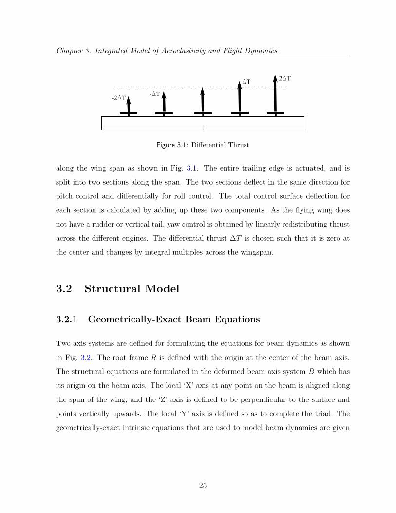
Figure 3.1: Differential Thrust
along the wing span as shown in Fig. 3.1. The entire trailing edge is actuated, and is
split into two sections along the span. The two sections deflect in the same direction for
pitch control and differentially for roll control. The total control surface deflection for
each section is calculated by adding up these two components. As the flying wing does
not have a rudder or vertical tail, yaw control is obtained by linearly redistributing thrust
across the different engines. The differential thrust ∆T is chosen such that it is zero at
the center and changes by integral multiples across the wingspan.
3.2 Structural Model
3.2.1 Geometrically-Exact Beam Equations
Two axis systems are defined for formulating the equations for beam dynamics as shown
in Fig. 3.2. The root frame R is defined with the origin at the center of the beam axis.
The structural equations are formulated in the deformed beam axis system B which has
its origin on the beam axis. The local ‘X’ axis at any point on the beam is aligned along
the span of the wing, and the ‘Z’ axis is defined to be perpendicular to the surface and
points vertically upwards. The local ‘Y’ axis is defined so as to complete the triad. The
geometrically-exact intrinsic equations that are used to model beam dynamics are given
25

Chapter 3. Integrated Model of Aeroelasticity and Flight Dynamics
Figure 3.2: Beam Axis system
by [77]:
F′ + (k + κ)F + f = P + ΩP (3.1)
M′ + (k + κ)M + (e1 + ε)F + m = H + ΩH + VP (3.2)
where at any point on the beam axis, F and M represent the forces and moments re-
spectively on the cross-section, k represents the curvature of the undeformed beam, ε
and κ represent the generalized strains and curvatures, f and m represent the external
forces and moments per unit span respectively, P and H represent the linear and angular
momentum respectively, V and Ω represent the linear and angular velocity respectively,
and e1 represents the unit vector [1 0 0]T . The generalized strain ε and curvature κ are
26

Chapter 3. Integrated Model of Aeroelasticity and Flight Dynamics
defined as [77],
ε = CBb(e1 + bu′ + bkbu)− e1
κ = BK− bk
where
BK = −CBb′CbB + CBbbkCbB
CBb represents the rotation matrix from the undeformed local frame b to the deformed
local frame B and bu represents the measure numbers of the displacement of a point on
the beam axis in the undeformed local frame b.
In the above equations, the operator ( )′ represents a derivative along the local X
axis, ( ˙ ) represents a time derivative in the local frame and the (˜) operator is defined
for a vector v as,
v =
0 −v3 v2
v3 0 −v1
−v2 v1 0
These equations for dynamics of the beam are augmented by the following intrinsic
kinematic equations which relate the variation of linear and angular velocity along the
wing span to the time-rate of change of strain and curvature [78]:
V′ + (k + κ)V + (e1 + ε)Ω = ε (3.3)
Ω′ + (k + κ)Ω = κ (3.4)
The spatial derivatives in the above equations are of order one, which is the lowest possible
order.
27

Chapter 3. Integrated Model of Aeroelasticity and Flight Dynamics
The position vector of a point on the deformed beam axis in the root frame (rB) and
the rotation of the local B frame relative to the R frame (CBR) can be obtained using,
r′B = CRB(ε+ e1) (3.5)
CBR′ = −(κ+ k)CBR (3.6)
Using a small-strain and slender beam assumption, the strains and curvatures are
related to the internal forces and moments using the following linear relation [7]:εκ =
R S
ST T
F
M
(3.7)
For an isotropic beam which has the shear center and tension axis coincident with the
reference axis, the constitutive relation is given in the local frame by [78],
ε1
ε2
ε3
κ1
κ2
κ3
=
1/EA 0 0 0 0 0
0 1/k2GA 0 0 0 0
0 0 1/k3GA 0 0 0
0 0 0 1/GJ 0 0
0 0 0 0 1/EI2 0
0 0 0 0 0 1/EI3
F1
F2
F3
M1
M2
M3
(3.8)
where ε1 represents the extensional strain, and ε2, ε3 represent the transverse shear strain
measures of the reference line. κ1, κ2, κ3 represent the curvature of the beam under tor-
sional and bending loads. G represents the shear modulus, E represents Young’s modulus,
J represents the torsional constant, I2 and I3 represent the area moment of inertia along
the local Y and Z direction, k2 and k3 represent the shear correction factor and A repre-
sents the cross-sectional area.
The equations relating the linear and angular momentum with the linear and angular
28

Chapter 3. Integrated Model of Aeroelasticity and Flight Dynamics
velocities can be written as: P
H
=
µI −µξ
µξ I
V
Ω
(3.9)
where µ represents the sectional mass per unit length, I represents a 3×3 identity matrix,
ξ represents the position vector of the sectional center of gravity and I represents the
sectional moment of inertia matrix.
Equivalence to Equations for Rigid Body Modes
The equations for rigid body modes can be separated and obtained from Eqs. (3.1) and
(3.2) as follows. Since both equations are written in the local frame, pre-multiply all
terms by CRB to obtain components in the root frame, and integrate in the root frame
along the beam axis.
b∫0
(CRBF′ + CRB(k + κ)F + CRBf
)dx =
b∫0
CRB(P + ΩP
)dx
b∫0
(CRBM′ + CRB(k + κ)M + CRB(e1 + ε)F + CRBm
)dx =
b∫0
CRB(H + ΩH
)dx
+
b∫0
CRBVPdx (3.10)
Differentiate the matrix identity CBRCRB = I along the beam axis, and re-arranging terms,
we obtain,
CRB ′ = −CRBCBR′CRB
29

Chapter 3. Integrated Model of Aeroelasticity and Flight Dynamics
Substituting the expression for CBR′ from Eq. (3.6), CBR′ can be written as,
CRB ′ = CRB(k + κ) (3.11)
Substituting Eq. (3.5) and (3.11) in Eqn. (3.10) and rewriting time derivatives in the
inertial frame, the equations can be written as,
b∫0
((CRBF
)′+ CRBf
)dx =
b∫0
CRB ddt
I
Pdx (3.12)
b∫0
((CRBM
)′+ r′B × CRBF + CRBm
)dx =
b∫0
CRB ddt
I
Hdx+
b∫0
CRBVPdx (3.13)
Write the position vector rB of any point on the beam from the origin of the root axis
in terms of the position of the center-of-gravity of the airplane from the origin ξB and
the position vector of the point from the center-of-gravity rcgB . Since the derivative of ξB
along the beam axis is zero, the following expressions are obtained.
rB = ξB + rcgB
r′B = rcgB′
Take the cross-product of each term inside the integral in Eq. (3.12) with rcgB and add to
Eq. (3.13) to obtain,
b∫0
((CRBF
)′+ CRBf
)dx =
d
dt
I
b∫0
CRBPdx (3.14)
b∫0
((CRBM
)′+(rcgB × C
RBF)′
+ CRBm + rcgB × CRBf
)dx =
b∫0
d
dt
I
CRBHdx
+
b∫0
CRBVPdx+
b∫0
(rcgB ×
d
dt
I
CRBP
)dx (3.15)
30

Chapter 3. Integrated Model of Aeroelasticity and Flight Dynamics
The integral of the total linear momentum along the beam axis can be written in
terms of the total mass of the airplane and the velocity of the center of gravity as,
b∫0
CRBPdx = MtotalRVcg (3.16)
The velocity of any point on the beam V can be broken up into the velocity of the center-
of-gravity of the airplane Vcg and the relative velocity of the point with respect to the
center-of-gravity Vrel. The second term on the right hand side of Eq. (3.15) can now be
written as,
b∫0
CRBVPdx = RVcg ×b∫
0
CRBPdx+
b∫0
RVrel × CRBPdx =
b∫0
d
dt
I
rcgB × CRBPdx
Since the sectional forces F and moments M at both free ends of the beam are zero,
Eqs. (3.14)-(3.15) can be written as,
Rftotal =d
dt
I
MtotalRVcg (3.17)
Rmcgtotal =
d
dt
I
b∫0
(RH + rcgB ×
RP)dx (3.18)
Equivalence to Linear Structural Dynamics Equations
Standard linear equations for structural dynamics of beams in bending and torsion can be
obtained from Eqs. (3.1) and (3.2). Neglecting non-linear terms, these equations reduce
to,
F′ + f = µV (3.19)
M′ + e1F + m = IΩ (3.20)
31

Chapter 3. Integrated Model of Aeroelasticity and Flight Dynamics
Assuming the external bending moment per unit length [m2 m3] and the bending moment
of inertia [I2 I3] to be zero, the following six equations are obtained,
F1′ + f1 = µV1 (3.21)
F2′ + f2 = µV2 (3.22)
F3′ + f3 = µV3 (3.23)
M1′ +m1 = I1Ω1 (3.24)
M2′ − F3 = 0 (3.25)
M3′ + F2 = 0 (3.26)
The linearized versions of the kinematic equations given in Eqs. (3.1) and (3.2) are,
V′ + e1Ω = ε (3.27)
Ω′ = κ (3.28)
Ignoring shear deformation, the above equations can be combined with the constitutive
relations given in Eq. (3.8) to give,
EAV1′ = F1 (3.29)
V2′ − Ω3 = 0 (3.30)
V3′ + Ω2 = 0 (3.31)
GJΩ1′ = M1 (3.32)
EI2Ω2′ = M2 (3.33)
EI3Ω3′ = M3 (3.34)
Eqs. (3.22)-(3.23) and (3.25)-(3.26) together give linear equations for structural dy-
32

Chapter 3. Integrated Model of Aeroelasticity and Flight Dynamics
namics in bending, and are identical to the equations derived by Meirovitch [81],
− ∂2M3
∂x2+ f2 = µ
∂V2
∂t(3.35)
∂2M2
∂x2+ f3 = µ
∂V3
∂t(3.36)
The above equations can be differentiated with respect to time, and combined with
Eqs. (3.30)-(3.31) and Eqs. (3.33)-(3.34) to give,
− ∂2
∂x2
(EI3
∂2V2
∂x2
)+ f2 = µ
∂2V2
∂t2(3.37)
− ∂2
∂x2
(EI2
∂2V3
∂x2
)+ f3 = µ
∂2V3
∂t2(3.38)
Eq. (3.21) and (3.24) correspond to the equations for structural dynamics in the axial
and torsional mode respectively. These equations can be combined with Eqs.(3.29) and
(3.32) to give,
∂
∂x
(EA
∂V1
∂x
)+ f1 = µ
∂2V1
∂t2(3.39)
∂
∂x
(GJ
∂Ω1
∂x
)+ m1 = I1
∂2Ω1
∂t2(3.40)
Finite difference discretization
Consider a vector X. Denote the nodal values of the vector by Xnl and Xn
r , where the
superscript denotes the node number, the subscript denotes the left or right side of the
node, and the hat denotes that it is nodal value. For the nth element,the spatial derivative
and the mean value over the element are given by,
X′ =Xn+1l − Xn
r
dl(3.41)
X = Xn
=Xn+1l + Xn
r
2(3.42)
33
Chapter 3. Integrated Model of Aeroelasticity and Flight Dynamics
Eqs.(3.1)-(3.4) are re-written in discretized form as,
Fn+1l − Fn
r
dl+ (κn + kn)F
n+ f
n − Pn − Ω
nPn
= 0 (3.43)
Mn+1l − Mn
r
dl+ (κn + kn)M
n+ (e1 + εn)F
n+ mn − H
n − ΩnHn − V
nPn
= 0 (3.44)
Vn+1l − Vn
r
dl+ (κn + kn)V
n+ (e1 + εn)Ω
n − εn = 0 (3.45)
Ωn+1l − Ωn
r
dl+ (κn + kn)Ω
n − κn = 0 (3.46)
This discretization scheme was found to be second-order accurate along the length of
the beam [78]. In addition, it satisfies both conservation integrals presented in the paper
relating to the change in generalized momentum and change in total mechanical energy.
3.2.2 Gravitational Model
The force and moment due to gravitational effects are modeled as
fg = µg (3.47)
mg = µξg (3.48)
where g is the gravity vector. The components of g are known in the inertial frame.
The components of the gravity vector g in the deformed frame at all the nodes can be
calculated using the following equations:
g′ + (κ+ k)g = 0 (3.49)
g + Ωg = 0 (3.50)
34

Chapter 3. Integrated Model of Aeroelasticity and Flight Dynamics
which in the discretized form can be written as
gn+1l − gnrdl
+ (κn + kn)gn = 0 (3.51)
˙g +˜Ωg = 0 (3.52)
In the above set of equations, the time-differentiated one is satisfied at one reference
node; following which the spatially-differentiated equation can be used to obtain com-
ponents of the g vector at other nodes. Each equation represents a set of three scalar
equations. Since the magnitude of the g vector is a constant (represented by g0), one
of the three dynamic equations is replaced by this magnitude constraint. The dynamic
equation at the reference node ng is re-written as
(e1eT1 + e2e
T2 ) ˙g
ng+ (e1e
T1 + e2e
T2 )˜Ωng
gng + e3|gng | = e3g0 (3.53)
3.2.3 Propulsive Model, nodal masses, and slope discontinuities
To account for the presence of nodal mass, nodal force (thrust) and slope discontinuities
the internal force on one side of the node is modeled as being different from the internal
force on the other side of the node. Thus the nodal equations are,
Fnr − Cn
T
lr Fnl + fnT + µngnr −
˙Pnr −
˜Ωnr P
nr = 0 (3.54)
Mnr − Cn
T
lr Mnl + mn
T + µn˜ξngnr −
˙Hnr −
˜Ωnr H
nr −
˜Vn
r Pnr = 0 (3.55)
where fnT is the discrete nodal thrust force defined in the reference frame corresponding to
the right side of the node, mnT is the corresponding nodal moment, µn is the concentrated
nodal mass, and ξn is the corresponding mass offset. Pnr and Hn
r are the linear and angular
35

Chapter 3. Integrated Model of Aeroelasticity and Flight Dynamics
momenta of the concentrated modal mass, given byPnr
Hnr
=
µnI −µn ˜ξnµn˜ξn In
Vnr
Ωnr
+
0
Hnengine
(3.56)
where In is the mass moment of inertia matrix of the nodal mass and Hnengine is the angular
momentum of the engine.
A discontinuity in the slope of the beam at the node is accounted for using the
following expressions,
Vnl = CnlrVn
r (3.57)
Ωnl = CnlrΩn
r (3.58)
gnl = Cnlrgnr (3.59)
The vectors Vnl , Ωn
l and gnl can now be replaced by Vnr , Ωn
r and gnr , thus reducing the
number of variables.
3.3 Aerodynamic Model
The aerodynamic forces and moments acting on the wing are computed using Peters
and Johnson’s two dimensional unsteady airloads model [79]. The sectional forces and
moments are written as,
fnaero =ρcn
2
0
f2
f3
mnaero =
ρcn2
2
m1
0
0
36

Chapter 3. Integrated Model of Aeroelasticity and Flight Dynamics
where,
f2 = −(CnL0
+ CnLδδn)V n
T Vna3
+ CnLα(V n
a3+ λn0 )2 − Cn
D0V nT V
na2
f3 = (CnL0
+ CnLδδn)V n
T Vna2− Cn
LαVna3
cn
4− Cn
LαVna2
(V na3
+ λn0 − Ωna1
cn
4)− Cn
D0V nT V
na3
m1 = (Cnm0
+ Cnmδδn)V n
T2 − Cn
mαVnT V
na3− cn
2
(CnLα
8+Cnpitch
2
)V na2Ωn
a1− cn2Cn
Lα
Ωna1
128
+cnCnLα
V na3
32(3.60)
Vna represents the velocity components at the mid-chord of the nth element. λn0 represents
the downwash due to free vorticity for the nth element and is computed using an inflow
model. The velocity components at the mid-chord are computed as,
Vna = CnTa V
n − ymc × CnT
a Ωn
Ωna = CnTa Ω
n
V nT =
√V 2a2
+ V 2a3
(3.61)
where Cna represents the rotation matrix from the local aerodynamic to the local structural
axis system. These forces and moments are re-written in the beam reference axes as,
fn
aero = Cna fnaero
mnaero = Cnamn
aero + Cna ynacfnaero (3.62)
The inflow λn0 in Eq. (3.60) is computed using Peters 2D inflow model [80]:
[Ainflow] λn+
(2V n
T
cn
)λn =
(−V n
a3+cn
4Ωna1
)cinflow (3.63)
λn0 =1
2binflowTλn (3.64)
37

Chapter 3. Integrated Model of Aeroelasticity and Flight Dynamics
where the coefficients are constant matrices derived in Ref. [80]. Six states are used in
the vector λn for the nth element, and the vector binflow is computed using an augmented
least-squares expansion.
3.4 Aeroelastic Equations
The final equations in discretized form are a collection of equations presented above. These
consist of the primary equations for each element Eqs. (3.43)-(3.46) and Eq. (3.51), the
equations at each node Eqs. (3.54)-(3.55) and the equations for unsteady aerodynamics
Eq. (3.63).
The following boundary conditions complete the set of equations required to analyze
the free-flying aircraft problem as formulated above:
F1l = 0 (3.65)
M1l = 0 (3.66)
FN+1r = 0 (3.67)
MN+1r = 0 (3.68)
(e1eT1 + e2e
T2 ) ˙g
ng+ (e1e
T1 + e2e
T2 )˜Ωng gng + e3(|gng | − g0) = 0 (3.69)
N denotes the total number of elements and ng denotes the reference node for gravity.
3.5 Open-loop Trim Computation and Linear Stabil-
ity Analysis
The trim state of the system is specified in terms of the flight speed, the flight path
angle, and the rate of turn in the inertial frame. Sideslip is constrained to be zero. The
38

Chapter 3. Integrated Model of Aeroelasticity and Flight Dynamics
corresponding equations for specifying these quantities are given by,
Vng2
1 + Vng2
2 + Vng2
3 − V 2∞ = 0 (3.70)
Ωngr .(g
ngr /g0)− ri = 0 (3.71)
Vng
1 gng1 + V
ng2 g
ng2 + V
ng3 g
ng3 + V∞g0 sin γ = 0 (3.72)
Vng
1 = 0 (3.73)
The set of equations presented in Section (3.4) along with the four constraint equations
present above constitute a set of non-linear equations in the state variables ( Vnr , Ωn
r , Fnl ,
Fnr , Mn
l , Mnr , gnr , n = 1 . . . N + 1) from the structural model, (λn, n = 1 . . . N) from the
unsteady aerodynamic model, and thrust, flap, aileron deflection and differential thrust
corresponding to the trim point. These non-linear equations are solved using the Newton-
Raphson method to compute the trim point, in terms of the thrust T , flap δf , aileron
deflection δa and the differential thrust ∆T . Following trim computation, the equations
are linearized at the trim point. Linear stability analysis is carried out by computing the
eigenvalues of the system. These eigenvalues indicate the stability of the system for small
perturbations about the trim point.
To identify the effect of static aeroelastic deformation on the flight dynamics, the
curvature of the flying wing at trim is used to define the shape of an equivalent rigid flying
wing. Flight dynamic eigenvalues for the equivalent rigid configuration are computed and
compared with those of the complete flight dynamic/aeroelastic system.
3.6 Non-dimensional form and aeroelastic parame-
ters
Eqs. (3.1)-(3.2) are non-dimensionalized to obtain parameters that determine the inter-
action of aeroelasticity with flight dynamics. The first equation is divided by qc and the
39

Chapter 3. Integrated Model of Aeroelasticity and Flight Dynamics
second equation is divided by qc2 to re-write the equations as
∂F∂ζ
(l
c
)+ (kl + κl)F
(l
c
)+ CF +
(µg
qc
)=∂P∂τ
+ ωP (3.74)
∂M∂ζ
(l
c
)2
+ (kl + κl)M(l
c
)2
+ (e1 + ε)F(l
c
)2
+ CM +
(µξg
qc2
)=∂H∂τ
+ ωH + VP
(3.75)
where, F = F/ql2, M = M/ql3, P = PV∞/qc2, H = HV∞/qc
3, ζ = x/l, τ = tV∞/c,
ω = Ωc/V∞, V = V/V∞.
The nondimensional forms of Eqs. (3.7)-(3.9) are given by, ε
κl
=
(ql2)R (ql3)S
(ql3)ST (ql4)T
FM (3.76)
PH =
2I(µ/ρc2) −2(µ/ρc2)(ξ/c)
2(µ/ρc2)(ξ/c) 2(I/ρc4)
Vω (3.77)
The matrices R and S in Eqs. (3.76)-(3.77) are set to zero as the average shear strain
across the cross section is negligible and the average normal strain is negligible. If the
structural axis system coincides with the beam principal axis, the matrix T is diagonal
with elements [1/GJ, 1/(EI)y, 1/(EI)z]. When non-dimensionalized as (ql4)T , the diago-
nal elements consist of the aeroelastic parameters ql4/GJ, ql4/(EI)y, ql4/(EI)z. These
parameters, along with elements of square matrix in Eq. (3.77), can be used as a met-
ric to quantify static aeroelastic deformation at trim. Similar parameters were defined
to ensure aeroelastic similitude while predicting free-flight and flutter characteristics of
airplanes from flexible test models [82].
40
Chapter 4
Control System Design
4.1 Overview
The objective of the control system is to track a pre-defined trajectory on the ground while
maintaining a specified flight speed and altitude. This is accomplished by a combination of
a non-linear guidance algorithm [83] and a multi-loop dynamic inversion controller [84, 85]
applied to the equations of motion of the flexible airplane written in the mean axis system.
The use of the mean axis system to write the equations of motion eliminates the coupling
between the rigid body modes and the structural dynamics of the deformed airplane [9],
resulting in a reduced-order system with only six degrees-of-freedom. The effect of static
aeroelastic deformation on the flight dynamics, which will be shown to be significant in
the next chapter, is accounted for by recalculating the center-of-gravity and the total
moment-of-inertia of the airplane at every time instant. Dynamic inversion applied to
this six degree-of-freedom reduced-order model of the statically deformed airplane cancels
out the nonlinear flight dynamics and replaces it with prescribed dynamics.
41

Chapter 4. Control System Design
4.2 Mean Axis Model
The concept of the mean axis was used by Milne to study the dynamics of a deformable
airplane by assuming small deformation[9]. The mean axis system is defined as a system
with respect to which the motion due to deformation has zero linear and angular momen-
tum. If small deformation is assumed, this use of the mean axis system decouples the
equations for flight dynamics from the equations for structural dynamics. In the follow-
ing sections, the equations for flight dynamics are derived in the mean axis for a generic
discretized model without making a small deformation assumption, and the corresponding
mean axes parameters are computed from the aeroelastic state vector for the flying wing.
4.2.1 Equations of Motion
Figure 4.1: Axis system
Consider a set of infinitesimal rigid bodies each with its associated local reference
frame B as shown in Fig. 4.1. Represent the mass of the nth body by µn and the moment of
inertia matrix in the local frame by BIn. The corresponding velocity vector is represented
42

Chapter 4. Control System Design
in the local frame by BVn, and the angular velocity of the rigid body by BΩn. Represent
the forces and moments acting on each rigid body in the local frame by Bfn and Bmn
respectively. Define a non-inertial reference frame O whose origin is at a distance RO
from the origin of the inertial reference frame I. The position of the the nth body in the
O frame is represented by rn, and in the inertial frame by Rn. These three vectors are
now related by,
Rn = RO + rn
The total linear momentum of the set of bodies in the O frame is now given by,
OP =∑
µnd
dt
I
ORn =∑
µnCOBnBVn (4.1)
which can also be written as,
OP =∑
µnd
dt
I
(ORO + Orn)
=∑
µnd
dt
I
ORO +∑
µnd
dt
I
Orn
= MtotalOVO +
∑µn
d
dt
I
Orn (4.2)
where Mtotal is the total mass of the system and OVO represents the velocity of the origin
of the O frame. Representing the position of the center of gravity of the set of bodies in
the O frame by OξO, the following relation can be obtained.
∑µn
d
dt
I
Orn =d
dt
I
∑µnOrn =
d
dt
I
MtotalOξO
Eq. (4.2) can now be written as
OP = MtotalOVO +Mtotal
OξO + OΩO ×MtotalOξO (4.3)
43

Chapter 4. Control System Design
The expression for the total angular momentum in the O frame is given by,
OHO =∑
Orn × µn ddt
I
ORn +∑COBnBInBΩn
=∑
Orn × µnCOBnBVn +∑COBnBInBΩn (4.4)
An alternate expression for the angular momentum is given by,
OHO =∑
Orn × µn ddt
I
(ORO + Orn) +∑COBnBInBΩn
=∑
µnOrn × d
dt
I
ORO +∑
Orn × µn ddt
I
Orn +∑COBnBInBΩn
= MtotalOξO × OVO +
∑Orn × µn d
dt
O
Orn +∑
Orn × µn(OΩO × Orn)
+∑COBnBInBΩn
= MtotalOξO × OVO +
∑Orn × µn d
dt
O
Orn + OIOOΩO
+∑COBnBInBΩn (4.5)
where the inertia matrix IO is given by
OIO =∑
µn((Orn · Orn)I− OrnOrn
)(4.6)
The rate of change of linear momentum is given by,
d
dt
I
OP =∑
µnd2
dt2
I
ORn =∑COBnBfn (4.7)
An alternate expression is given by,
d
dt
I
OP =d
dt
O
OP + OΩO × OP
= MtotalOVO +Mtotal
OξO + OΩO ×MtotalOξO + OΩO ×Mtotal
OξO
+OΩO × OP (4.8)
44

Chapter 4. Control System Design
The rate of change of angular momentum is given by,
d
dt
I
OHO =∑ d
dt
I
Orn × µn ddt
I
ORn +∑
Orn × µn d2
dt2
I
ORn
+∑COBn d
dt
I
BInBΩn
=∑ d
dt
I
(ORn − ORO
)× µn d
dt
I
ORn +∑
Orn × COBnBfn
+∑COBnBmn
= − d
dt
I
ORO ×∑
µnd
dt
I
ORn +∑
Orn × COBnBfn +∑COBnBmn
= −OVO × OP +∑
Orn × COBnBfn +∑COBnBmn (4.9)
An alternate expression is given by,
d
dt
I
OHO =d
dt
O
OHO + OΩO × OHO
= MtotalOξO × OVO +Mtotal
OξO × OVO +∑
Orn × µn d2
dt2
O
Orn
+∑(
Orn × µn(OΩO × Orn) + Orn × µn(OΩO × Orn))
+∑
Orn × µn(OΩO × Orn) +∑COBnBInBΩn + OΩO × OHO
= MtotalOξO × OVO +Mtotal
OξO × OVO +∑
Orn × µn d2
dt2
O
Orn
+OIOOΩO + OIOOΩO + OΩO × OHO
+∑COBnBInBΩn +
∑COBnBInBΩn (4.10)
where
OIO =∑
µn(2(Orn · Orn
)I− OrnOrn − OrnOrn
)(4.11)
COBn = COBnBΩn − OΩOCOBn
(4.12)
The expression for COBn is obtained from Ref. [77].
45

Chapter 4. Control System Design
Now place the origin of the frame O at the center of gravity of the system. The
subscript O on the right-hand side of velocity, moment-of-inertia and angular momentum
is now changed to cg to denote the shift of origin to the center of gravity. This sets the
vector OξO and the corresponding rate term to zero. Eqs. (4.1) and (4.3) now give the
expression for velocity of the center of gravity as,
OVcg =1
Mtotal
∑µnCOBnBVn (4.13)
This prescribes the translational velocity of the origin of the O frame. Placing the origin
of the O frame at the center-of-gravity of the system ensures that the linear momentum
due to deformation is zero in the O frame.
Eqs. (4.4) and (4.5) when equated can be used to obtain multiple solutions to the
angular velocity OΩO. Choosing the angular velocity of the O frame to be,
OΩM = OI−1cg
∑Orn × µnCOBnBVn (4.14)
implies,
∑Orn × µn d
dt
O
Orn = 0
This choice of angular velocity of the O frame ensures that the deformation motion has
zero angular momentum in the O frame. If the linear and angular velocity of the O
frame are calculated as shown in Eqs. (4.13) and (4.14) respectively, the axis system O
corresponds to the mean axis system M [9].
Eqs. (4.7) and (4.8) give the force equation as,
MtotalOVcg + OΩM × OP =
∑COBnBfn (4.15)
46

Chapter 4. Control System Design
and Eqs. (4.9) and (4.10) give the moment equation as
OIcgOΩM + OIcgOΩM + OΩM × OHcg =∑
Orn × COBnBfn +∑COBnBmn
−∑COBnBInBΩn −
∑COBnBInBΩ
n(4.16)
where OP and OHcg are calculated as shown in Eq. (4.1) and (4.4) respectively.
Eqs. (4.15)-(4.16) represent the equations of motion of the mean axis system with
its origin at the center-of-mass of the system of bodies. If the relative position of the
rigid bodies does not vary significantly, OIcg can be approximated to be equal to zero. If
the system of rigid bodies is taken to be a finite-state representation of a flexible body,
Eqs. (4.15)-(4.16) represent the flight dynamics equations that are decoupled from the
equations for structural dynamics under the small-deformation assumption. However, it
is important to note that these equations are not completely decoupled due to the coupling
through aerodynamic forces and moments.
4.2.2 Application to current problem
Calculation of the mean axis parameters for the flying wing problem are carried out in the
root axis system R whose origin is at the center of the airplane on the beam X axis. The
forces and moments acting on each element, and the corresponding masses and moments
of inertia are split into two equal halves and lumped at the nodes on the ends of each
element. The expressions for these quantities are given by,
µn =µndl
2+µn−1dl
2+ µn
BξnB =1
µn
(µndlξ
n
2+µn−1dlCnTlr ξ
n−1
2+ µnξn
)BIn =
Indl2
+CnTlr I
n−1Cnlrdl2
+ In + Iµn + CnTlr Iµn−1Cnlr
47

Chapter 4. Control System Design
Bfn =fn
aerodl
2+CnTlr f
n−1
aerodl
2+ fnT
Bmn =mn
aerodl
2+CnTlr mn−1
aerodl
2+ mn
T
Iµn = µn
ξn2dl/2 −ξndl2/8 0
−ξndl2/8 dl3/24 0
0 0 (dl3/24) + (ξn2dl/2)
where BξB is position of center-of-mass of the total nodal mass.
The aeroelastic state vector contains the nodal velocities and angular velocities at
the origin of the local frame B. The velocity at the mass position is given in terms of the
nodal velocity and angular velocity as,
BVn = Vnr + Ωn
r × BξnB
BΩn = Ωnr (4.17)
Eqs. (3.5)-(3.6) can be discretized and used to obtain the nodal positions on the beam
axis from the origin of the root frame rnB and rotations of the deformed beam at the node
CRBn in terms of the strains and curvatures as,
CBRn+1
=
(∆
dl+κn
+ kn
2
)−1(∆
dl− κ
n+ kn
2
)CBRn (4.18)
rn+1B = rnB +
(CBRn + CnlrCBR
n+1)T
(εn + e1)dl/2 (4.19)
The above expression can now be used to obtain the position of the total mass at the nth
node relative to the center-of-gravity as,
Rrn = rnB + CRBnBξnB − Rξcg (4.20)
It is to be noted that Eq. (4.16) which is the moment equation acting on the total airplane
48

Chapter 4. Control System Design
uses(rnB − Rξcg
), as the total moment acting at the node Bmn is calculated at the origin
at the local frame. All other expressions for Orn in section 4.2.1 are to be substituted by
Rrn.
4.2.3 Kinematic Equations
For designing the control system, three axis systems are necessary. These are the root
axis system R, shown in Fig. 3.2, an inertial axis system I with the same arrangement of
axes, and the mean axis system M . The relative orientation of both the mean and the
root axis system relative to the inertial axis system is defined using a 3−1−2 Euler angle
rotation sequence. The corresponding rotation matrices are given below for reference:
C3(ψ) =
cosψ sinψ 0
− sinψ cosψ 0
0 0 1
C1(θ) =
1 0 0
0 cos θ sin θ
0 − sin θ cos θ
C2(φ) =
cosφ 0 − sinφ
0 1 0
sinφ 0 cosφ
The rotation matrices can now be defined as,
CMI = C2(φmi)C1(θmi)C3(ψmi)
CRI = C2(φri)C1(θri)C3(ψri)
CMR = CMICRIT (4.21)
The rate of change of Euler angles is related to the inertial components of the angular
velocity vector by, φ
θ
ψ
=
− sinψ sec θ cosψ sec θ 0
cosψ sinψ 0
sinψ tan θ − cosψ tan θ 1
IΩ (4.22)
49

Chapter 4. Control System Design
The inertial position of the center of gravity is related to the root axis components
of velocity by,
I xcg = CIRRVcg (4.23)
4.3 Control System Design
4.3.1 Guidance Algorithm
The nonlinear guidance algorithm used in this dissertation for path following was devel-
oped by Park et al. [83]. This guidance law was shown to give superior performance as
compared to linear guidance laws in following curved paths. This is due to its ability to
calculate the required lateral acceleration based on the commanded path ahead of the
current vehicle position, and the use of the inertial velocity in calculating the acceleration
to compensate for external disturbances such as wind [83].
Figure 4.2: Guidance Algorithm
Consider a trajectory defined by a sequence of points in the inertial frame as shown
in Fig. 4.2. Denote the current inertial co-ordinates of the airplane by (x,y,h). Select a
reference point on the trajectory at a specified distance L1 ahead of the current position.
Let Vg represent the velocity of the airplane in the XIY I plane and η represent the angle
50

Chapter 4. Control System Design
between the velocity vector and the line to the reference point. The guidance algorithm
gives the demanded lateral acceleration as [83],
adl = 2Vg
2
L1
sin η (4.24)
The lookforward distance L1 also gives a lower bound on the radius of the circular ground
path that can be followed as L1/2 [83].
4.3.2 Review of Dynamic Inversion
Theoretical Foundations
Application of linear control theory to non-linear problems requires the system to be
linearized at multiple operating points. Controllers designed at each operating point
using linear control theory can then be combined by specifying the gains as function of
the operating point (gain-scheduling algorithms). However, gain-scheduling can be tedious
and may be impossible to implement if nonlinearities are present in multiple variables. On
the other hand, dynamic inversion controllers work by canceling the inherent dynamics of
selected control variables (CVs) over the entire domain and replacing them with desired
dynamics [86].
Consider a system whose dynamics can be represented in the form,
x = f(x) + g(x)u (4.25)
where x ∈ Rn represents the state vector and u ∈ Rm represents the control vector. Let
the vector of CVs be given by,
y = h(x) (4.26)
51

Chapter 4. Control System Design
where, y ∈ Rk.
The rate of change of CVs is given by,
y =dh
dxx =
dh
dx(f(x) + g(x)u)
= F(x) + G(x)u (4.27)
G(x) is invertible if the number of CVs is equal to the number of states in the control
input u. Now, if G(x) is invertible, select the vector of control inputs u such that,
u = G−1(ydes − F(x)) (4.28)
where ydes represents the desired dynamics of the CVs. The control inputs give us the
desired dynamics. The CVs have to be selected and the desired dynamics of the CVs’
have to be specified as part of the control design process.
The choice of CVs is critical to the performance of the dynamic inversion controller.
The dynamics of the states which are not controlled by the control input defined in
Eq. (4.28) are known as zero dynamics. For the closed loop system to give the desired
performance, CVs have to be selected such that the zero dynamics are stable [87].
A fundamental assumption in dynamic inversion is that Eqs. (4.25)-(4.26) represent
the dynamics of the system exactly [88]. Uncertainty in the model will have to be ac-
counted for by using robust control design techniques. In general, dynamic inversion
controllers do not require a gain scheduling algorithm. Exceptions to this occur when
commanded control inputs are large enough to cause actuator saturation [88].
Method of Multiple Time-Scales
Flight dynamics for a conventional rigid airplane configuration are modeled by a set of
eight first order differential equations. The state vector x consists of velocity V , flight
52

Chapter 4. Control System Design
path angle γ, angle of attack α, side-slip angle β, body-axis roll angle φ, body-axis roll rate
p, body-axis pitch rate q and body-axis yaw rate r. The control vector u consists of thrust
T , and control surface deflections δe, δa, δr for elevator, aileron and rudder respectively.
If the CV vector y in Eq. (4.26) is taken to be the state vector x, then the system is
required to have as many elements in the control vector u as there are in the state vector
x for G(x) to be invertible. Since this is not the case for a typical airplane, a two-step
approach has been devised which makes use of the multiple time-scales inherent in the
dynamics of the system [84, 85]. Ref. [88, 89] present a good review of Dynamic Inversion
as applied to the airplane control problem.
4.3.3 Control Architecture for Flying Wings
The dynamic inversion controller is designed using the force equation given by Eq. (4.15),
the moment equation given by Eq. (4.16) and the kinematic equation given below:MΩM 1
MΩM 2
MΩM 3
=
0 cosφmi − sinφmi cos θmi
1 0 sin θmi
0 sinφmi cosφmi cos θmi
φmi
θmi
ψmi
(4.29)
Applying the method of multiple time scales, the equations are inverted sequentially,
and the output of inversion from one step is fed into the next. This procedure is repre-
sented schematically in Fig. 4.3.
The inputs given to the controller are the commanded velocity Vc, commanded alti-
tude hc and commanded ground path in terms of the inertial X −Y co-ordinates (xc, yc).
These inputs are used in the first step to compute the demanded lateral acceleration and
the commanded flight path angle γc. Based on the current position, ground speed and
a pre-specified length, the guidance algorithm is used to compute the demanded lateral
acceleration. The magnitude of this demanded lateral acceleration is given by Eq. (4.24),
53
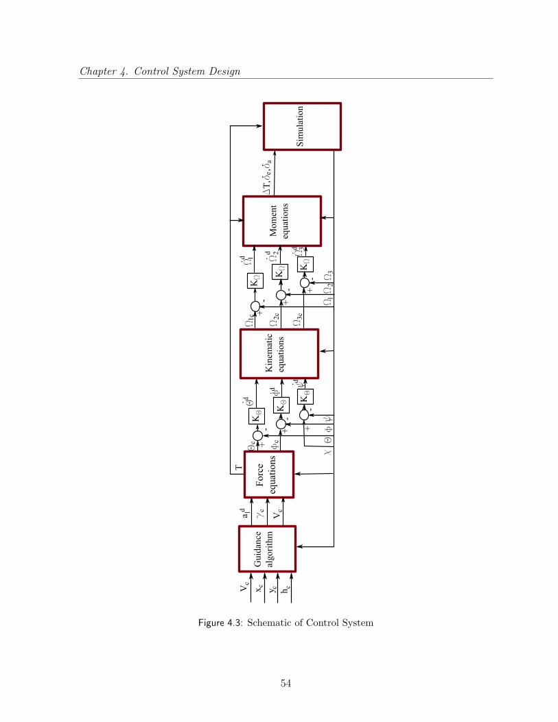
Chapter 4. Control System Design
Figure 4.3: Schematic of Control System
54

Chapter 4. Control System Design
and it is oriented in the direction normal to the projection of velocity vector in the inertial
XIY I plane as shown in Fig. 4.2. The commanded flight path angle γc is calculated as,
γc =(hc − h)
Lh(4.30)
where Lh is the reference length in the ZI−V∞ plane. This demanded lateral acceleration
is specified in an intermediate frame V which is offset from the inertial frame by a rotation
χ about the ZI axis. The components of the acceleration in the V frame are given by,
V ad =
adl
0
0
(4.31)
In the second step, the force equations in Eq. (4.15) are inverted to find the magni-
tude of thrust required and the commanded pitch and roll angles, while holding constant
the commanded velocity along the inertial Z axis (Vc sin γc) and inertial X − Y plane
(Vc cos γc). The accelerations in the mean axis system are given by,
MVcg + MΩMMVcg = CMV V ad (4.32)
where the accelerations V ad are computed in the previous step and the rotation matrix
CMV is given by,
CMV = C2(φmi)C1(θmi)C3(ψmi + χ) (4.33)
Eq. (4.15) is non-linear in T , θ and φ and is solved using a Newton-Raphson solver to
obtain commanded values of thrust T , pitch angle θmic and roll angle φmic . In order to
solve this set of nonlinear equations, the velocity and angular velocity at any spanwise
location has to be expressed as function of Vc cos γc and Vc sin γc and the angular velocity
of the mean axis. This is done using Eqs. (3.45)-(3.46) while setting the rates εn and
55

Chapter 4. Control System Design
κn to zero. This is equivalent to assuming that the structure of the flying wing is rigid
with its shape being the instantaneous deformed shape, and that aerodynamic forces and
moments generated by structural vibrations are ignored. These new velocity and angular
velocity values, which correspond to the motion of a deformed, rigid flying wing are used
in the controller to compute aerodynamic forces and moments.
In the next step, the demanded roll, pitch and yaw rates are prescribed as,
φdmi = Kθ(φmic − φmi) (4.34)
θdmi = Kθ(θmic − θmi) (4.35)
ψdmi = −Kθ(χ+ ψmi) (4.36)
The dynamics are prescribed such that the controller tries to drive the states to the
prescribed values with a time-constant that is inversely proportional to the gain Kθ.
These three rates are used to compute the commanded angular velocities MΩMc using
Eq. (4.29).
In the final step, the demanded angular velocity rates are computed as,
MΩdM = KΩ(MΩMc − MΩM) (4.37)
RΩdM and Eq. (3.46) is used to compute the BΩn term present in Eq. (4.16). Eq. (4.16) is
inverted to find the differential thrust required for yaw control, and the required aileron
and flap deflections.
4.4 Time-marching Implementation
A set of non-linear equations given by,
[M] x = f(x) (4.38)
56

Chapter 4. Control System Design
can be discretized for time-marching as,
[M]xt+∆t − xt
∆t= f(αxt + βxt+∆t) (4.39)
The above set of discretized equations represent a forward-difference scheme for α =
1, β = 0, a backward-difference scheme for α = 0, β = 1 and a central-difference scheme
for α = 0.5, β = 0.5. The explicit forward-difference scheme is unstable and first-order
accurate, while the implicit backward-difference scheme is first-order accurate and damps
out high frequency oscillations. The central difference scheme is implicit, second-order
accurate and energy conserving. The energy-conserving nature of the central-difference
scheme may cause it to become unstable due to oscillations whose time periods are much
smaller than the time-step of the simulation. In addition, the accuracy of these higher
order modes is dependent on the spatial discretization of the finite-difference scheme used
in this dissertation.
Therefore, time marching is implemented in this dissertation by setting α = 0.495, β =
0.505 and time step of ∆t = 0.02s. The choice of α and β damps out high frequency
oscillations while giving almost second-order accuracy. Given xt, Eq. (4.39) now represents
an implicit, non-linear set of equations in xt+∆t, which is solved for using a Newton-
Raphson solver.
For the closed-loop system, this time-marching algorithm is implemented at each
time-step on two sets of equations. The first set corresponds to the complete aeroelastic
model given by Eqs. (3.43)-(3.46), (3.51), (3.54)-(3.55) and (3.63) which has (21×N) +
((N − 1) ×m) states, where N corresponds to the number of nodes and m corresponds
to the number of unsteady aerodynamic states at each element. The second set consists
of kinematic equations given by Eq. (4.22) applied to both the root and the mean axis,
and Eq. (4.23) applied to the center-of-gravity of the flying wing.
57

Chapter 4. Control System Design
4.5 Overview of Closed-Loop Simulation
Figure 4.4: Closed-Loop Schematic
The schematic of the closed-loop system is shown in Fig. 4.4. Given a state vector
of the complete aeroelastic system at time t, a module computes the velocity, angular
velocity, linear and angular momentum, and moment of inertia at that time instant in
the mean axis. These values, together with the inertial position and Euler angles, are
used to compute the control input to be applied to the system from time t to t + ∆t.
The time-marching algorithm described in the previous section is used to compute the
aeroelastic state vector at time t+ ∆t using the state vector at the previous time instant
and the control input. Concurrently, the velocity of the center of gravity and the angular
velocity of the mean axis are used to obtain the inertial co-ordinates and the Euler angles
at time t+ ∆t.
58

Chapter 4. Control System Design
4.6 State Estimation for Control
The controller design presented in this chapter requires nodal values of velocities Vnr ,
angular velocities Ωnr , nodal positions with respect to the origin of the root frame rn, ro-
tation of the local frame with respect to the root frame CRBn and unsteady aerodynamic
states λ for load calculation. Nodal positions and rotations of the local frame were com-
puted from the nodal strains and curvatures at each time step as shown in Eqs. (4.18) and
(4.19). However, the nodal values of velocity, angular velocity and unsteady aerodynamic
states were directly extracted from the aeroelastic state variable at that time instant. As
the aeroelastic state vector will not be available when the controller is implemented on
a real airplane, unsteady aerodynamic states will have to be simulated on-board using
Eq. (3.63) for each element before the loads can be computed. Nodal velocities and angu-
lar velocities will have to be calculated in terms of the corresponding values at the wing
root using the following expressions obtained by rewriting Eqs. (3.45) and (3.46):
(∆
dl+˜κn+1
l + kn
2
)Cn+1lr Ωn+1
r =
(∆
dl−˜κnr + kn
2
)Ωnr
+˙κn+1
l + ˙κn
r
2(∆
dl+˜κn+1
l + kn
2
)Cn+1lr Vn+1
r +˜εn+1
l + e1
2Cn+1lr Ωn+1
r =
(∆
dl−˜κnr + kn
2
)Vnr
−˜εnr + e1
2Ωnr +
˙εn+1
l + ˙εn
r
2(4.40)
59

Chapter 5
Results
5.1 Open Loop Verification
Table 5.1: Geometric parameters for Goland Wing
b = 6.096 m CL0 = 0 CLα = 2π CLδ = 1 CD0 = 0.0c = 1.829 m Cm0 = 0 Cmα = 0 Cmδ = −0.25 µ = 35.71 kg/m
Ixx = 8.641 kg m Iyy = 0.0 kg m Izz = 8.641 kg m
Table 5.2: Elastic parameters for Goland Wing
Number of nodes 41Sectional center of gravity 43% chord
Elastic axis position 33% chordTorsional Rigidity 0.987× 10⁶ N m2
Bending Rigidity 9.77× 10⁶ N m2
The open loop aeroelastic code has been verified for a number of test cases against
standard results. Boundary conditions presented in Eq. (3.65)-(3.69) are changed to
simulate a cantilevered beam case by specifying the velocity, angular velocity and pitch
angle at the root. Flutter prediction results from the code are compared with results from
60

Chapter 5. Results
analytical computational percentage differenceFlutter Velocity 137.16 m/s 136.22 m/s 0.68 %
Frequency 70.685 rad/s 70.063 rad/s 0.88 %Free-vibration 1st mode 49.492 rad/s 49.502 rad/s 0.02 %bending 2nd mode 310.16 rad/s 310.90 rad/s 0.24 %frequencies 3rd mode 868.46 rad/s 874.07 rad/s 0.65 %
Divergence velocity 252.39 m/s 250.82 m/s 0.62 %Control reversal velocity 141.38 m/s 141.40 m/s 0.01 %
Euler buckling load 648.93 kN 649.10 kN 0.03 %Tip moment for circle 100.73 kNm 100.94 kNm 0.002 %
Table 5.3: Verification results
−5 0 5 10 15 20−15
−10
−5
0
5
x axis
z ax
is
Beam deformation with increasing tip moment
Figure 5.1: Test for geometric exactness
an analytical model for the Goland wing [90, 91] whose parameters are given in Table 5.1
and 5.2. Free-vibration bending frequencies, Euler buckling loads, divergence velocity and
control reversal velocity are compared with analytical results for a modified Goland wing,
which has its sectional center of mass relocated to the beam elastic axis. These results
are presented in Table 5.3. Application of a sufficiently large moment about the Y axis
61

Chapter 5. Results
at the tip of the beam is seen to deform the beam into a circle as shown in Fig. 5.1, thus
verifying geometric exactness of the beam model. The bending rigidity of the beam is
decreased to 9.77× 10⁴ N m2 for the test for geometric exactness.
3 3.5 4 4.5−6
−5
−4
−3
−2
−1
0
1
log of number of nodes
log
of %
err
or
Modal frequency convergence plot
1st mode frequency
2nd mode frequency
3rd mode frequency
Figure 5.2: Error Convergence plot for bending frequencies
Fig. 5.2 plots the log of the percentage error between the computed and analytical
bending frequencies for the cantilevered beam versus the log of the number of the nodes.
The plots for all the three modes show a slope of negative two. This implies that the
percentage error in the computed frequency decreases with an increase in number of
nodes, and that the percentage error is inversely proportional to the square of the number
of nodes.
5.2 Open Loop Dynamics
A sample configuration is used to study both open and closed loop characteristics of the
flying wing. Parametric values used to define the configuration are given in Tables 5.4
62
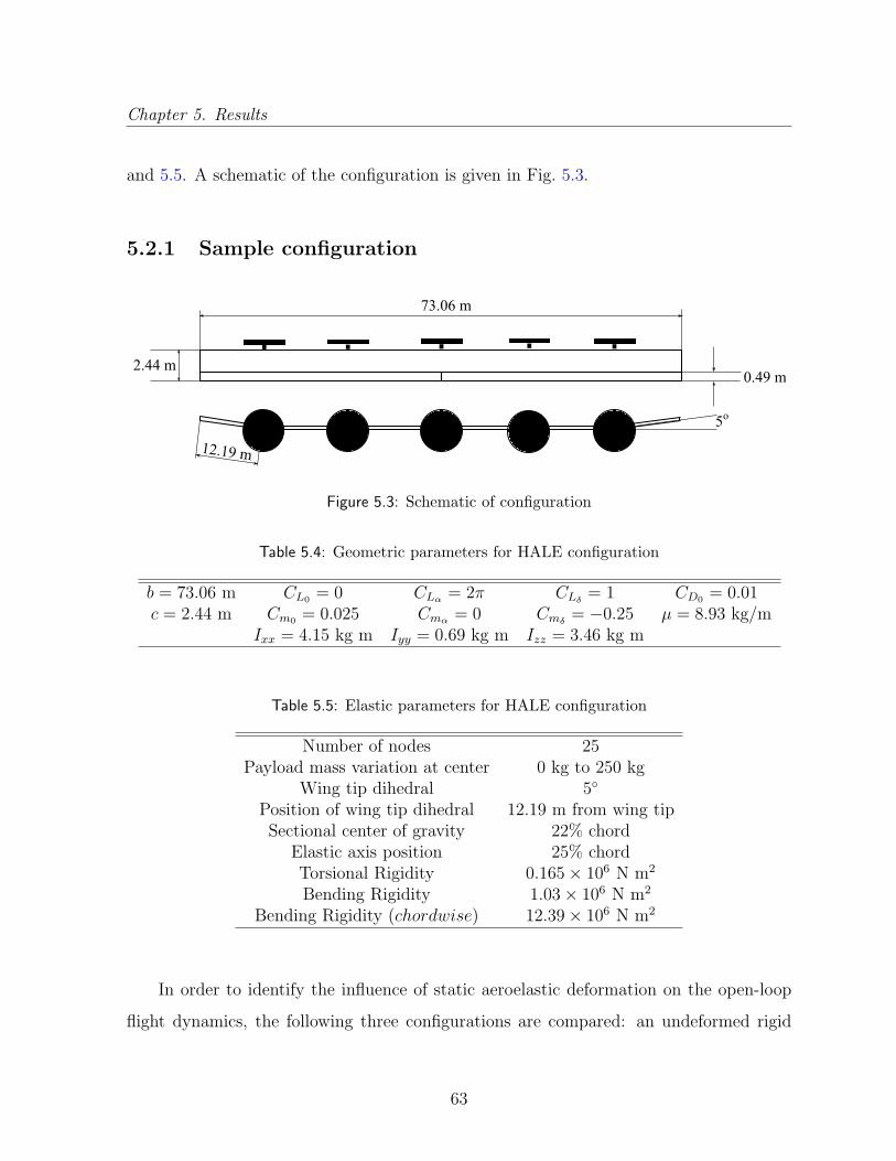
Chapter 5. Results
and 5.5. A schematic of the configuration is given in Fig. 5.3.
5.2.1 Sample configuration
Figure 5.3: Schematic of configuration
Table 5.4: Geometric parameters for HALE configuration
b = 73.06 m CL0 = 0 CLα = 2π CLδ = 1 CD0 = 0.01c = 2.44 m Cm0 = 0.025 Cmα = 0 Cmδ = −0.25 µ = 8.93 kg/m
Ixx = 4.15 kg m Iyy = 0.69 kg m Izz = 3.46 kg m
Table 5.5: Elastic parameters for HALE configuration
Number of nodes 25Payload mass variation at center 0 kg to 250 kg
Wing tip dihedral 5
Position of wing tip dihedral 12.19 m from wing tipSectional center of gravity 22% chord
Elastic axis position 25% chordTorsional Rigidity 0.165× 10⁶ N m2
Bending Rigidity 1.03× 10⁶ N m2
Bending Rigidity (chordwise) 12.39× 10⁶ N m2
In order to identify the influence of static aeroelastic deformation on the open-loop
flight dynamics, the following three configurations are compared: an undeformed rigid
63

Chapter 5. Results
flying wing (UNDEFORMED), a rigid flying wing defined using static aeroelastic defor-
mation at trim for a given flight condition (DEFORMED), and a flexible flying wing
configuration (FLEXIBLE). Open-loop analysis is carried out in two steps: trim compu-
tation, followed by linear stability analysis.
5.2.2 Trim Computation
A comparison of control parameters at straight and level trim for the UNDEFORMED
and FLEXIBLE configuration was carried out by Patil and Hodges [7], and has not been
repeated here. The trim computed for the FLEXIBLE configuration is used to defined
the rigid body shape for the DEFORMED configuration. This section presents control
parameters computed for four different trim states for the FLEXIBLE/DEFORMED con-
figuration.
Figs. 5.4-5.8 shows the variation of control parameters with nodal mass at the center
(payload) for four different trim cases. These consist of a straight and level trim at 12.19
m/s at sea-level, a straight climb at 12.19 m/s at a 2 slope, a level turn at 12.19 m/s
with a radius of 6096 m, and a helical climbing turn at 12.19 m/s with a 2 slope and a
radius of 6096 m. Increasing the payload mass at the center increases the net bending
moment acting on the wing, leading to a larger bending deformation and a corresponding
decrease in local angle of attack on the outboard wing sections. This effect is reflected in
the variation of the required angle of attack at the root and the required aileron deflection
with increasing payload mass.
As previously observed in Ref. [7], the variation in thrust required for straight and
level trim is not found to vary significantly with the payload mass. This is attributed to
the fact that the 2D aerodynamic model assumes a constant CD0 . The thrust required
for climbing flight with a 2 flight path angle increases linearly with nodal mass. This is
consistent with the aircraft performance equation which shows that excess thrust required
for climb increases linearly with aircraft weight for a given flight path angle [92].
64

Chapter 5. Results
0 50 100 150 200 2500
20
40
60
80
100
Nodal mass at center in kg
Tri
m T
hrus
t in
N
Trim Thrust variation with nodal mass
level trim2° climblevel turnclimbing turn
Figure 5.4: Trim Thrust variation with nodal mass
0 50 100 150 200 2500
1
2
3
4
5
6
7
Nodal mass at center in kg
Roo
t ang
le−
of−
atta
ck in
deg
rees
Root angle−of−attack variation with nodal mass
level trim2° climblevel turnclimbing turn
Figure 5.5: Root angle-of-attack variation with nodal mass
65
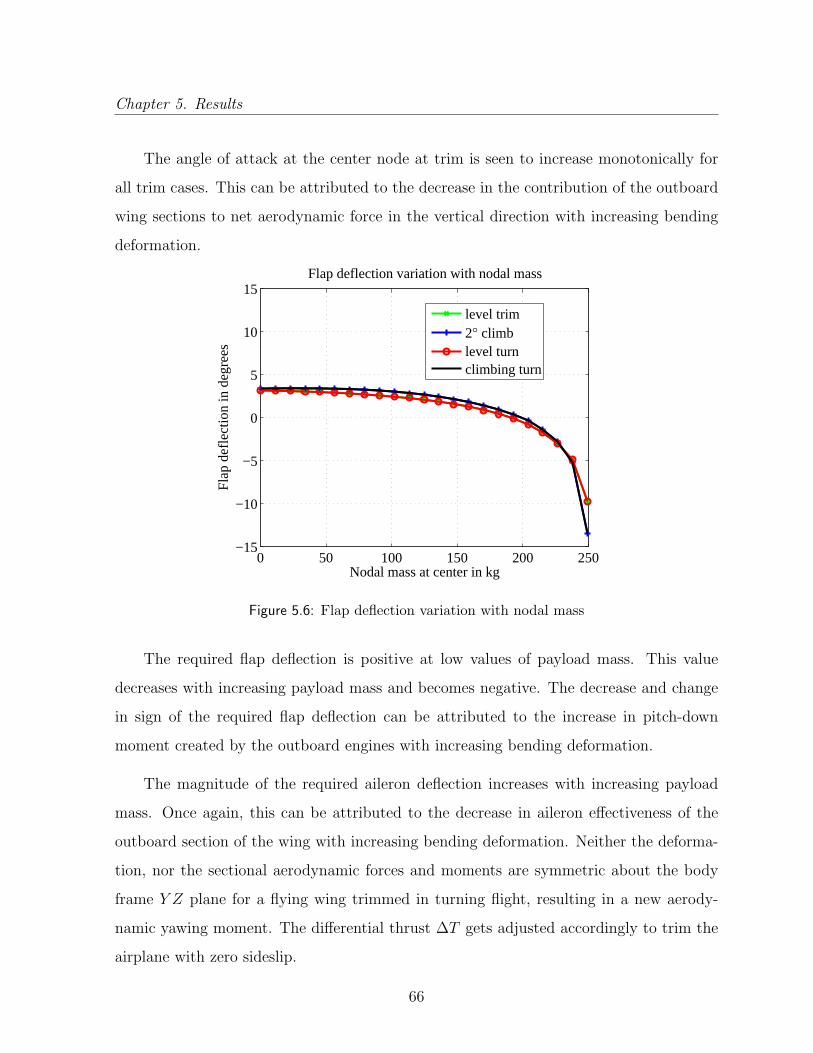
Chapter 5. Results
The angle of attack at the center node at trim is seen to increase monotonically for
all trim cases. This can be attributed to the decrease in the contribution of the outboard
wing sections to net aerodynamic force in the vertical direction with increasing bending
deformation.
0 50 100 150 200 250−15
−10
−5
0
5
10
15
Nodal mass at center in kg
Flap
def
lect
ion
in d
egre
es
Flap deflection variation with nodal mass
level trim2° climblevel turnclimbing turn
Figure 5.6: Flap deflection variation with nodal mass
The required flap deflection is positive at low values of payload mass. This value
decreases with increasing payload mass and becomes negative. The decrease and change
in sign of the required flap deflection can be attributed to the increase in pitch-down
moment created by the outboard engines with increasing bending deformation.
The magnitude of the required aileron deflection increases with increasing payload
mass. Once again, this can be attributed to the decrease in aileron effectiveness of the
outboard section of the wing with increasing bending deformation. Neither the deforma-
tion, nor the sectional aerodynamic forces and moments are symmetric about the body
frame Y Z plane for a flying wing trimmed in turning flight, resulting in a new aerody-
namic yawing moment. The differential thrust ∆T gets adjusted accordingly to trim the
airplane with zero sideslip.
66

Chapter 5. Results
0 50 100 150 200 250−1.4
−1.2
−1
−0.8
−0.6
−0.4
−0.2
0
Nodal mass at center in kg
Aile
ron
defl
ectio
n in
deg
rees
Aileron deflection variation with nodal mass
level turn
climbing turn
Figure 5.7: Aileron deflection variation with nodal mass
0 50 100 150 200 250−1
−0.5
0
0.5
1
Nodal mass at center in kg
Δ T
hrus
t in
N
Δ Thrust variation with nodal mass
level turn
climbing turn
Figure 5.8: ∆ Thrust variation with nodal mass
67

Chapter 5. Results
5.2.3 Linear Stability Analysis for Straight and Level Trim
This section looks at the variation of dutch roll, phugoid and spiral eigenvalues with the
nodal mass at the center of the flying wing. The root locus plots for the eigenvalues are
obtained by varying the nodal mass from 0 kg to 249.47 kg. The eigenvalues correspond-
ing to the 0 kg case are indicated by green squares on the root locus plots, while the
eigenvalues corresponding to the 249.47 kg case are indicated by green triangles. The
roll mode and short period mode couple with the unsteady aerodynamic modes in the
UNDEFORMED and DEFORMED configuration and with the aeroelastic modes in the
FLEXIBLE configuration and are not studied in this section. The dutch roll and the
phugoid mode exhibit dynamic instability as the nodal mass at the center of the wing is
increased. This onset of dynamic instability in the FLEXIBLE configuration is captured
by the DEFORMED configuration but not by the UNDEFORMED configuration. Static
stability characteristics are studied in Section 5.2.5.
−0.1 −0.05 0 0.05 0.1 0.15 0.2 0.25−0.8
−0.6
−0.4
−0.2
0
0.2
0.4
0.6
0.8Root locus plot for Phugoid
FLEXIBLEDEFORMEDUNDEFORMED
Figure 5.9: Root locus plot for Phugoid
68

Chapter 5. Results
The root locus plot for the phugoid mode is shown in Fig. 5.9. For both the FLEX-
IBLE and DEFORMED configuration, the phugoid mode is seen to go unstable with
increasing payload mass, though the UNDEFORMED configuration remains stable as
seen in Fig. 5.9. More significantly, the phugoid mode corresponding to the FLEXIBLE
configuration goes unstable near the mass value at which the phugoid mode of the DE-
FORMED configuration crosses the zero damping line. Table 5.6 shows eigenvalues for
phugoid modes for two values of payload, denoted by ‘light’ (45.35 kg) and ‘heavy’ (181.4
kg) respectively.
‘light’ payload (45.35 kg) ‘heavy’ payload (181.4 kg)UNDEFORMED Phugoid −0.0773± 0.4509 i −0.0775± 0.5052 iDEFORMED Phugoid −0.0672± 0.4572 i 0.1049± 0.5754 iFLEXIBLE Phugoid −0.0689± 0.4596 i 0.0981± 0.6235 i
Table 5.6: Longitudinal Eigenvalues
−0.4 −0.3 −0.2 −0.1 0 0.1
−0.4
−0.2
0
0.2
0.4
0.6Root locus plot for Lateral−Directional modes
FLEXIBLEDEFORMEDUNDEFORMED
Figure 5.10: Root locus plot for Lateral-Directional modes
The root locus plot for lateral-directional modes is plotted in Fig. 5.10. For lateral-
69

Chapter 5. Results
−0.025 −0.02 −0.015 −0.01 −0.005 0 0.005
−0.4
−0.2
0
0.2
0.4
0.6Root locus plot for Dutch Roll
FLEXIBLEDEFORMEDUNDEFORMED
Figure 5.11: Root locus plot for Dutch roll mode
directional modes, the eigenvalues of the DEFORMED configuration are seen to track
those of the FLEXIBLE configuration. The dutch roll mode is seen to go unstable with
increasing payload mass in Fig. 5.11. Once again, it is seen that the instability in the dutch
roll mode in the FLEXIBLE configuration is captured by the DEFORMED configuration,
but not by the UNDEFORMED configuration. The spiral mode is seen to be stable for
the entire range of nodal mass for all three configurations. Table 5.7 shows eigenvalues
for lateral-directional modes for the ‘light’ and ‘heavy’ payload cases.
‘light’ payload (45.35 kg) ‘heavy’ payload (181.4 kg)UNDEFORMED Dutch Roll −0.0045± 0.1410 i −0.0043± 0.1410 i
Spiral −0.1559 −0.2060DEFORMED Dutch Roll −0.0016± 0.2003 i 4.2488e− 005± 0.3499 i
Spiral −0.1587 −0.2392FLEXIBLE Dutch Roll −0.0028± 0.1987 i 0.0044± 0.3654 i
Spiral −0.1925 −0.2616
Table 5.7: Lateral-Directional Eigenvalues
70

Chapter 5. Results
5.2.4 Stability Boundary for Straight and Level Trim
−0.02 0 0.02 0.04 0.06 0.08 0.1 0.120
20
40
60
80
100
position of CG relative to quarter−chord in m
noda
l mas
s at
cen
ter
in k
g
Stability Boundary for straight, level trim
DEFORMEDFLEXIBLE
Stable
Unstable
Unstable
Figure 5.12: Stability Boundary
For a flying wing trimmed in straight and level flight, Fig. 5.12 shows the dependence
of stability on the payload mass at the center node and position of chordwise sectional
center-of-gravity location. The DEFORMED rigid wing is seen to go unstable at a lower
payload value than the corresponding FLEXIBLE system for all chordwise positions of
center of gravity. For both configurations, the dutch roll mode is the one that goes
dynamically unstable at a lower payload (as compared to the phugoid mode) for the
entire center-of-gravity range. The discussion on static stability characteristics is given in
the next section.
5.2.5 Modified Static Stability Criteria
The criteria for static stability for longitudinal flight dynamics gets modified in the pres-
ence of significant structural deformation. Typically, airplanes show static stability in the
longitudinal plane if the chordwise CG location is ahead of the aerodynamic center. This
71
Chapter 5. Results
center of gravity position ensures that the aerodynamic pitching moment perturbation
resulting from a perturbation in angle of attack stabilizes the airplane. Mathematically,
this condition is expressed as,
(Cmα)cg < 0 (5.1)
The above condition assumes that the thrust does not induce a pitching moment, and
consequently the net pitching moment about the center-of-gravity at trim is purely aero-
dynamic in nature and is equal to zero. However, for configurations which undergo sig-
nificant structural deformation or have engines vertically offset from the center of gravity,
thrust does induce a pitching moment. In this case, the aerodynamic pitching moment
at trim about the center-of-gravity is non-zero. The condition for static stability gets
modified as,
(Cmα)cg − (Caerom )cg
CLαCL
< 0 (5.2)
The above condition can be obtained by assuming a non-zero aerodynamic pitching mo-
ment at trim, and computing the determinant of the coefficients of the four linearized
equations for dynamics in the longitudinal plane. For a given chordwise center-of-mass
location, the criteria obtained in Eq. (5.2) is found to predict the nodal mass value for the
onset of static instability for the DEFORMED configuration with an error of less than
1% and for the FLEXIBLE configuration with an error of 2%.
5.3 Closed Loop Dynamics
Changes to configuration
The configuration studied in the previous section was found to be susceptible to aileron
reversal. In this condition, the effect of aileron deflection is to induce a rolling moment
72
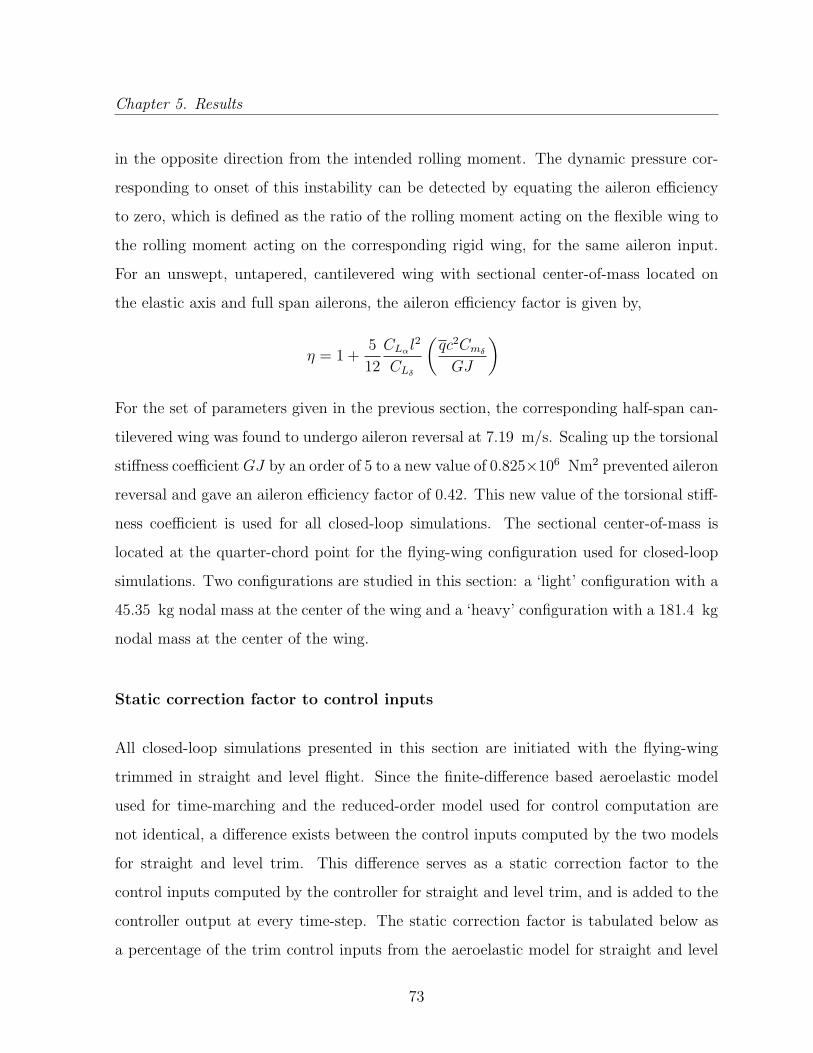
Chapter 5. Results
in the opposite direction from the intended rolling moment. The dynamic pressure cor-
responding to onset of this instability can be detected by equating the aileron efficiency
to zero, which is defined as the ratio of the rolling moment acting on the flexible wing to
the rolling moment acting on the corresponding rigid wing, for the same aileron input.
For an unswept, untapered, cantilevered wing with sectional center-of-mass located on
the elastic axis and full span ailerons, the aileron efficiency factor is given by,
η = 1 +5
12
CLαl2
CLδ
(qc2CmδGJ
)
For the set of parameters given in the previous section, the corresponding half-span can-
tilevered wing was found to undergo aileron reversal at 7.19 m/s. Scaling up the torsional
stiffness coefficient GJ by an order of 5 to a new value of 0.825×10⁶ Nm2 prevented aileron
reversal and gave an aileron efficiency factor of 0.42. This new value of the torsional stiff-
ness coefficient is used for all closed-loop simulations. The sectional center-of-mass is
located at the quarter-chord point for the flying-wing configuration used for closed-loop
simulations. Two configurations are studied in this section: a ‘light’ configuration with a
45.35 kg nodal mass at the center of the wing and a ‘heavy’ configuration with a 181.4 kg
nodal mass at the center of the wing.
Static correction factor to control inputs
All closed-loop simulations presented in this section are initiated with the flying-wing
trimmed in straight and level flight. Since the finite-difference based aeroelastic model
used for time-marching and the reduced-order model used for control computation are
not identical, a difference exists between the control inputs computed by the two models
for straight and level trim. This difference serves as a static correction factor to the
control inputs computed by the controller for straight and level trim, and is added to the
controller output at every time-step. The static correction factor is tabulated below as
a percentage of the trim control inputs from the aeroelastic model for straight and level
73

Chapter 5. Results
trim.
thrust flap deflection aileron deflection ∆ thrust‘light’ payload 1.60× 10⁻³% 1.46× 10⁻⁴% 0 % 0 %‘heavy’ payload 0.0364 % −4.65× 10⁻³% 0 % 0 %
Table 5.8: Static correction factor
Gain selection
For the multi-step dynamic inversion method used in this dissertation to work, it is
important to ensure that the time scale for the prescribed faster dynamics is higher than
the time scale for the prescribed slower dynamics. The equations for the rate of change
of angular velocity constitute the faster dynamics, and are the first ones to be addressed.
The selection of these gains is explained using the equation for the rate of change of
angular velocity along the XM axis. Since, the dynamic inversion controller inverts the
moment equation exactly the new dynamics for the rate of change of angular momentum
is given by Eq. (4.37) as,
M ΩM1 = M ΩdM1
= KΩ(MΩM1c −MΩM1) (5.3)
Assuming the roll angle φmi to be zero, Eq. (5.3) can be re-written using Eqs. (4.29)
and (4.35) as,
θmi = KΩ(Kθ(θmic − θmi)− θmi)
which gives the following second-order equation for θmi,
θmi +KΩθmi +KΩKθθmi = KΩKθθmic
The values of KΩ and Kθ are chosen to be 1 rad/s and 0.1 rad/s respectively, which
74

Chapter 5. Results
gives the following values for frequency and damping:
ωn =√KΩKθ = 0.316 rad/s
ζ =1
2
√KΩ
Kθ
= 1.581
For an overdamped second-order system, the time constant for the exponential decay of
the amplitude is given by 1/ζωn. This time constant can be used as the characteristic
time scale for the system response. For these gain values of KΩ and Kθ, this time scale
has a value of 2 s.
The time scales for the slow dynamics is determined by the guidance equations for
path-following and altitude change. The rate of change of altitude can be written using
Eq. (4.30) as,
h = Vc sin γc =VcLh
(hc − h)
The above first-order system has a time constant given by Lh/Vc. For a prescribed flight
speed of 12.19 m/s, the reference length Lh is chosen to be 1219 m, giving a time constant
of 100 s. The guidance law linearized for following a straight-line path becomes a second-
order equation in the lateral-offset distance, and has a frequency and damping value given
by [83],
ωn =
√2VcL1
ζ =1√2
= 0.707
For a lookforward length L1 of 1219 m, the characteristic time scale 1/ζωn has a value of
100 s. These gain values ensure sufficient separation between the time-scales for the fast
and slow dynamics, and are used in all simulations presented in this section.
75

Chapter 5. Results
5.3.1 Path-following for straight line path
Straight and level path with initial vertical offset
The first set of simulations are for straight climbing flight. The simulation is initialized
with the airplane trimmed in straight and level flight at 12.19 m/s along the inertial
Y axis at the origin of the inertial reference frame, and is commanded to increase its
altitude by 12.19 m while maintaining its heading. Two payload cases are considered:
the ‘light’ payload case corresponding to a nodal mass at the center of 45.35 kg and a
‘heavy’ payload case corresponding to a nodal mass of 181.4 kg. For each of the two
payload cases, simulations are presented for the fully flexible flying wing model (denoted
by ‘FLEXIBLE’ in the graphs) and a rigid body model based on the deformed shape
at straight and level trim (denoted by ‘DEFORMED’ in the graphs). Since the lateral
variables are unperturbed in this simulation, only the longitudinal variables have been
plotted in Figs. 5.13-5.14. These are the altitude of the airplane, the pitch angle of the
mean axis, the commanded thrust and the commanded flap deflection.
The altitude of the airplane shows a first-order response and converges to the com-
manded altitude. The pitch angle of the mean axis shows an initial perturbation during
climb before converging back the value for straight and level flight. The commanded
thrust value shows an abrupt jump at the very first time instant corresponding to the
step change in commanded altitude from the initial condition. The commanded flap de-
flection for the ‘FLEXIBLE’ configuration exhibits high frequency oscillations during the
transient response for both the ‘light’ and the ‘heavy’ payload cases due to an abrupt
change in commanded value. These oscillations are due to the coupling of the controller
with a low-frequency aeroelastic bending mode, and die out as time progresses. Even in
the presence of these oscillations, the mean value of the commanded flap deflection shows
the same trend as the commanded flap deflection for the corresponding ‘DEFORMED’
configuration.
76

Chapter 5. Results
0 200 400 600 800−2
0
2
4
6
8
10
12
14
time in s
heig
ht in
m
altitude in m
FLEXIBLE ‘light’FLEXIBLE ‘heavy’DEFORMED ‘light’DEFORMED ‘heavy’
(a) Altitude history
0 200 400 600 8002.8
3
3.2
3.4
3.6
3.8
4
4.2
4.4
time in s
θ in
°
Pitch angle
FLEXIBLE ‘light’FLEXIBLE ‘heavy’DEFORMED ‘light’DEFORMED ‘heavy’
(b) Pitch angle history
Figure 5.13: Straight and level path with initial vertical offset
77

Chapter 5. Results
0 200 400 600 80030
35
40
45
50
time in s
T in
N
Thrust
FLEXIBLE ‘light’FLEXIBLE ‘heavy’DEFORMED ‘light’DEFORMED ‘heavy’
(a) Thrust history
0 200 400 600 800
5
5.2
5.4
5.6
5.8
6
6.2
6.4
time in s
flap
in °
flap deflection
FLEXIBLE ‘light’FLEXIBLE ‘heavy’DEFORMED ‘light’DEFORMED ‘heavy’
(b) Flap history
Figure 5.14: Straight and level path with initial vertical offset
78

Chapter 5. Results
Straight and level path with initial lateral offset
The second set of simulations are for level flight with an initial lateral offset from the
commanded straight line path. The simulation is initialized with the airplane trimmed
in straight and level flight at 12.19 m/s along the inertial Y axis at (12.19, 0, 0) m in the
inertial reference frame, and the airplane is commanded to follow the inertial Y axis while
maintaining its altitude. As a consequence of the commanded trajectory and the initial
state, lateral dynamics of the flying wing are significant in this trajectory as compared
to longitudinal dynamics. Once again simulations are carried out for four cases: the
‘FLEXIBLE’ and ‘DEFORMED’ cases for both of the ‘light’ and ‘heavy’ payload. As both
the lateral and longitudinal variables are perturbed from their initial values, a complete
set of 9 parameters are plotted in Figs. 5.15-5.19. These are the altitude, lateral offset
(the inertial ‘x’ co-ordinate), roll angle of the mean axis, pitch angle of the mean axis,
yaw angle of the mean axis, commanded thrust, commanded flap deflection, commanded
aileron deflection and commanded ∆T .
After the initial transient response, the altitude of the airplane returns to its initial
value for all the four cases. The lateral offset shows a second order response with high
damping and the flight path of the airplane converges to the commanded ground path.
The roll and yaw angle are initialized as zero, and converge back to the same value
as the flight path converges to the commanded path. High frequency oscillations are
not observed in the commanded flap deflection for the ‘FLEXIBLE’ model as there is no
abrupt change in the commanded altitude. Both the aileron deflection and the differential
thrust value converge to zero after transients as the flight path of the airplane converges
to the commanded ground path.
79

Chapter 5. Results
0 200 400 600 800−2
0
2
4
6
8
10
12
14
time in s
x co
−or
d in
m
X co−ord
FLEXIBLE ‘light’FLEXIBLE ‘heavy’DEFORMED ‘light’DEFORMED ‘heavy’
(a) Ground track history
0 200 400 600 800−0.02
−0.015
−0.01
−0.005
0
0.005
0.01
0.015
0.02
time in s
heig
ht in
m
altitude in m
FLEXIBLE ‘light’FLEXIBLE ‘heavy’DEFORMED ‘light’DEFORMED ‘heavy’
(b) Altitude history
Figure 5.15: Straight and level path with initial lateral offset
80

Chapter 5. Results
0 200 400 600 8002.8
3
3.2
3.4
3.6
3.8
4
time in s
θ in
°
Pitch angle
FLEXIBLE ‘light’FLEXIBLE ‘heavy’DEFORMED ‘light’DEFORMED ‘heavy’
(a) Pitch angle history
0 200 400 600 800−0.015
−0.01
−0.005
0
0.005
0.01
time in s
φ in
°
Roll angle
FLEXIBLE ‘light’FLEXIBLE ‘heavy’DEFORMED ‘light’DEFORMED ‘heavy’
(b) Roll angle history
Figure 5.16: Straight and level path with initial lateral offset
81

Chapter 5. Results
0 200 400 600 800−0.1
0
0.1
0.2
0.3
0.4
0.5
0.6
time in s
ψ in
°
Yaw angle
FLEXIBLE ‘light’FLEXIBLE ‘heavy’DEFORMED ‘light’DEFORMED ‘heavy’
(a) Yaw angle history
0 200 400 600 80032.51
32.52
32.53
32.54
32.55
32.56
time in s
T in
N
Thrust
FLEXIBLE ‘light’FLEXIBLE ‘heavy’DEFORMED ‘light’DEFORMED ‘heavy’
(b) Thrust history
Figure 5.17: Straight and level path with initial lateral offset
82

Chapter 5. Results
0 200 400 600 800
5
5.2
5.4
5.6
5.8
6
6.2
time in s
flap
in °
flap deflection
FLEXIBLE ‘light’FLEXIBLE ‘heavy’DEFORMED ‘light’DEFORMED ‘heavy’
(a) Flap history
0 200 400 600 800−0.15
−0.1
−0.05
0
0.05
0.1
0.15
0.2
time in s
aile
ron
in °
aileron deflection
FLEXIBLE ‘light’FLEXIBLE ‘heavy’DEFORMED ‘light’DEFORMED ‘heavy’
(b) Aileron history
Figure 5.18: Straight and level path with initial lateral offset
83

Chapter 5. Results
0 200 400 600 800−0.3
−0.2
−0.1
0
0.1
0.2
0.3
0.4
0.5
time in s
Δ T
in N
Redistributed thrust
FLEXIBLE ‘light’FLEXIBLE ‘heavy’DEFORMED ‘light’DEFORMED ‘heavy’
Figure 5.19: Straight and level path with initial lateral offset
5.3.2 Path-following for curved ground path
The next two sets of simulations are for following a curved ground path. The commanded
path is defined to be a circle of fixed radius in the inertial XY plane. In order to study the
ground path of the airplane relative to its commanded path, a new parameter is plotted
for the next two sets of simulations. This new parameter ∆R is given by
∆R(t) = R(t)−Rc
where R(t) is given by,
R(t) =√
(x(t)− x0)2 + (y(t)− y0)2
In the above equations (x0, y0) represents the origin of the commanded flight path,
(x(t), y(t)) represent the inertial co-ordinates of the airplane and Rc represents the radius
of the commanded flight path.
84

Chapter 5. Results
Curved ground path with no initial offset
The simulation is initialized with the airplane trimmed in straight and level flight at
12.19 m/s along the inertial Y axis at the origin of the inertial co-ordinate system. The
airplane is commanded to track a circular ground path of radius 6096 m with an origin
at (6096, 0) m while maintaining its current altitude. Unlike the previous two cases, the
initial state of the flying wing and the final steady state correspond to two different trim
conditions for this trajectory. Once again due to the nature of this trajectory, the lateral
dynamics of the airplane are significant compared to the longitudinal dynamics. Both
the ‘light’ and the ‘heavy’ payload cases for the FLEXIBLE configuration are studied. A
total of ten parameters are plotted in Figs. 5.20-5.24. These are the ground path, ∆R,
altitude, pitch, roll and yaw angles of the mean axis, and the four control parameters.
For both the ‘light’ and the ‘heavy’ payload case, the parameter ∆R and the altitude
converge exactly to the commanded value. For both cases, the roll angle converges to a
non-zero value corresponding to banked flight, while the yaw angle increases linearly after
the transients die down. Though the airplane is commanded to maintain its altitude,
the longitudinal control variables (thrust and flap deflection) do not converge to their
initial value as the trim condition for turning flight is different from the trim for turning
flight. The aileron deflection and differential thrust ∆T converge to a non-zero value
corresponding to steady turning flight.
85

Chapter 5. Results
0 2000 4000 6000 8000 10000 12000−6000
−4000
−2000
0
2000
4000
6000
x co−ord in m
y co
−or
d in
m
ground track
FLEXIBLE ‘light’commanded trajectoryFLEXIBLE ‘heavy’
(a) Ground track history
0 200 400 600 800−5
0
5
10
15
20
25
time in s
Δ R
in m
Variation from radius of commanded path
FLEXIBLE ‘light’FLEXIBLE ‘heavy’
(b) ∆ R history
Figure 5.20: Curved ground path with no initial offset
86

Chapter 5. Results
0 200 400 600 800−0.02
0
0.02
0.04
0.06
0.08
0.1
time in s
heig
ht in
m
altitude in m
FLEXIBLE ‘light’FLEXIBLE ‘heavy’
(a) Altitude history
0 200 400 600 8002.8
3
3.2
3.4
3.6
3.8
4
4.2
time in s
θ in
°
Pitch angle
FLEXIBLE ‘light’FLEXIBLE ‘heavy’
(b) Pitch angle history
Figure 5.21: Curved ground path with no initial offset
87

Chapter 5. Results
0 200 400 600 800−0.05
0
0.05
0.1
0.15
0.2
0.25
0.3
time in s
φ in
°
Roll angle
FLEXIBLE ‘light’FLEXIBLE ‘heavy’
(a) Roll angle history
0 200 400 600 800−120
−100
−80
−60
−40
−20
0
20
time in s
ψ in
°
Yaw angle
FLEXIBLE ‘light’FLEXIBLE ‘heavy’
(b) Yaw angle history
Figure 5.22: Curved ground path with no initial offset
88

Chapter 5. Results
0 200 400 600 80032.35
32.4
32.45
32.5
32.55
32.6
time in s
T in
N
Thrust
FLEXIBLE ‘light’FLEXIBLE ‘heavy’
(a) Thrust history
0 200 400 600 800
5
5.2
5.4
5.6
5.8
6
6.2
time in s
flap
in °
flap deflection
FLEXIBLE ‘light’FLEXIBLE ‘heavy’
(b) Flap history
Figure 5.23: Curved ground path with no initial offset
89
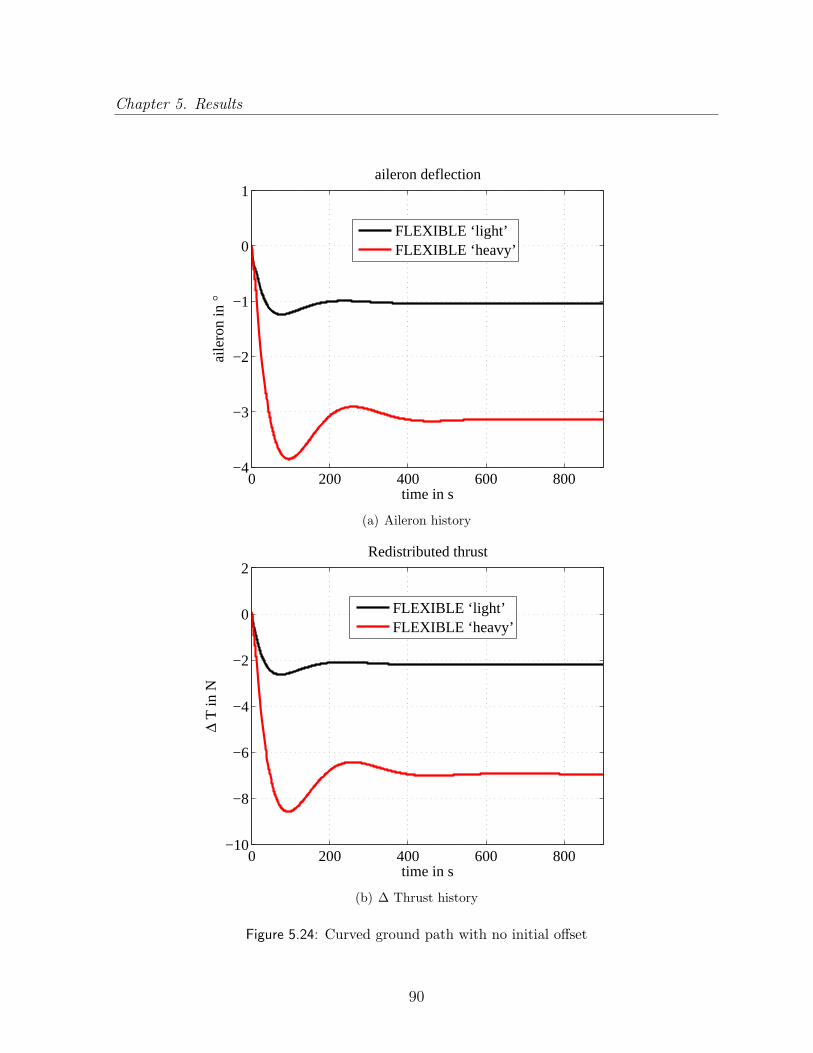
Chapter 5. Results
0 200 400 600 800−4
−3
−2
−1
0
1
time in s
aile
ron
in °
aileron deflection
FLEXIBLE ‘light’FLEXIBLE ‘heavy’
(a) Aileron history
0 200 400 600 800−10
−8
−6
−4
−2
0
2
time in s
Δ T
in N
Redistributed thrust
FLEXIBLE ‘light’FLEXIBLE ‘heavy’
(b) ∆ Thrust history
Figure 5.24: Curved ground path with no initial offset
90

Chapter 5. Results
Curved ground path with initial vertical and lateral offset
The simulation is initialized with the airplane trimmed in straight and level flight at
12.19 m/s along the inertial Y axis and with initial inertial co-ordinates of (12.19, 0, 0)
m. The airplane is commanded to track a circular path of radius 6096 m with an origin at
(6096, 0) m while increasing its altitude by 12.19 m. The commanded trajectory in this
case is a combination of the commanded trajectory in the previous three cases, and the
initial state and final steady state correspond to two different trim conditions. Both the
‘light’ and the ‘heavy’ payload cases for the FLEXIBLE configuration are studied. As in
the previous case, a total of ten parameters are plotted in Figs. 5.25-5.29.
The parameter ∆R converges to zero for both the ‘light’ and ‘heavy’ payload cases.
For both cases, the altitude converges to the commanded value of 12.19 m. The roll
angle converges to a non-zero value corresponding to a banked turn while the yaw angle
increases linearly with time. The commanded thrust and flap deflection converge to a
steady-state value once the commanded altitude is reached. As seen in the straight climb
case, the commanded flap deflection exhibits high frequency oscillations in the transient
phase due to coupling with an aeroelastic bending mode of the flexible flying wing. Once
again, the aileron and differential in thrust converge to non-zero values corresponding to
steady turning flight.
91

Chapter 5. Results
0 2000 4000 6000 8000 10000 12000−6000
−4000
−2000
0
2000
4000
6000
x co−ord in m
y co
−or
d in
m
ground track
FLEXIBLE ‘light’commanded trajectoryFLEXIBLE ‘heavy’
(a) Ground track history
0 200 400 600 800−15
−10
−5
0
5
10
15
20
time in s
Δ R
in m
Variation from radius of commanded path
FLEXIBLE ‘light’FLEXIBLE ‘heavy’
(b) ∆ R history
Figure 5.25: Curved ground path with initial vertical and lateral offset
92
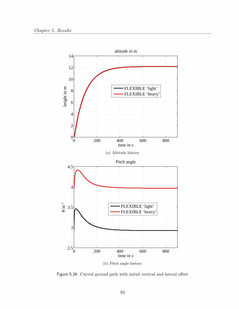
Chapter 5. Results
0 200 400 600 8000
2
4
6
8
10
12
14
time in s
heig
ht in
m
altitude in m
FLEXIBLE ‘light’FLEXIBLE ‘heavy’
(a) Altitude history
0 200 400 600 8002.5
3
3.5
4
4.5
time in s
θ in
°
Pitch angle
FLEXIBLE ‘light’FLEXIBLE ‘heavy’
(b) Pitch angle history
Figure 5.26: Curved ground path with initial vertical and lateral offset
93

Chapter 5. Results
0 200 400 600 800−0.05
0
0.05
0.1
0.15
0.2
0.25
0.3
time in s
φ in
°
Roll angle
FLEXIBLE ‘light’FLEXIBLE ‘heavy’
(a) Roll angle history
0 200 400 600 800−120
−100
−80
−60
−40
−20
0
20
time in s
ψ in
°
Yaw angle
FLEXIBLE ‘light’FLEXIBLE ‘heavy’
(b) Yaw angle history
Figure 5.27: Curved ground path with initial vertical and lateral offset
94
Chapter 5. Results
0 200 400 600 80030
35
40
45
50
time in s
T in
N
Thrust
FLEXIBLE ‘light’FLEXIBLE ‘heavy’
(a) Thrust history
0 200 400 600 800
5
5.2
5.4
5.6
5.8
6
6.2
6.4
time in s
flap
in °
flap deflection
FLEXIBLE ‘light’FLEXIBLE ‘heavy’
(b) Flap history
Figure 5.28: Curved ground path with initial vertical and lateral offset
95

Chapter 5. Results
0 200 400 600 800−4
−3
−2
−1
0
1
time in s
aile
ron
in °
aileron deflection
FLEXIBLE ‘light’FLEXIBLE ‘heavy’
(a) Aileron history
0 200 400 600 800−10
−8
−6
−4
−2
0
2
time in s
Δ T
in N
Redistributed thrust
FLEXIBLE ‘light’FLEXIBLE ‘heavy’
(b) ∆ Thrust history
Figure 5.29: Curved ground path with initial vertical and lateral offset
96

Chapter 5. Results
5.3.3 Extreme cases
This subsection studies the variation in the response of the closed loop system with
increasing lateral offset and climb altitude, and decreasing turn radius. As noted in
Section 3.1, the controller assumes a linear variation in ∆T across the five engines and
full span ailerons. The limits of the closed-loop system identified in this section will change
if this control distribution is changed. All simulations in this subsection are carried out
with a payload mass of 181.4 kg and initialized with the flying wing trimmed in straight
and level flight at 12.19 m/s along the inertial Y axis, unless specified otherwise.
Straight and level path with initial vertical offset
The first set of simulations looks at the response of the system to a commanded change
in altitude by 304.8 m and 152.4 m respectively while maintaining its heading. The
simulation is initialized with the airplane at the origin at the inertial reference frame. The
commanded altitude in subsection 5.3.1 was chosen to be 12.19 m and the corresponding
simulations are provided here as a reference.
Once again, the lateral states are not perturbed. The altitude of the airplane shows a
first-order response and converges to the commanded altitude. The time required for the
airplane to reach the commanded altitude for all three cases in found to be of the same
order. However this will no longer be true in a real system as constraints on the maximum
thrust of the engine are imposed. The jump in the commanded thrust at the very first
time instant increases with an increase in the commanded altitude. The commanded flap
deflections exhibit damped high frequency oscillations in the transient response due to
coupling with bending modes. The steady state values of the thrust, flap and pitch angle
converge to their initial values as these correspond to straight and level flight.
97

Chapter 5. Results
0 100 200 300 400 500 6000
50
100
150
200
250
300
350
time in s
heig
ht in
m
altitude in m
304.8 m climb152.4 m climb12.19 m climb
(a) Altitude history
0 100 200 300 400 500 6002
4
6
8
10
12
14
16
time in s
θ in
°
Pitch angle
304.8 m climb152.4 m climb12.19 m climb
(b) Pitch angle history
Figure 5.30: Straight and level path with initial vertical offset (large offsets)
98

Chapter 5. Results
0 100 200 300 400 500 6000
100
200
300
400
500
time in s
T in
N
Thrust
304.8 m climb152.4 m climb12.19 m climb
(a) Thrust history
0 100 200 300 400 500 6004
5
6
7
8
9
time in s
flap
in °
flap deflection
304.8 m climb152.4 m climb12.19 m climb
(b) Flap history
Figure 5.31: Straight and level path with initial vertical offset (large offsets)
99

Chapter 5. Results
Straight and level path with initial lateral offset
The next set of simulations studies the variation of the closed-loop response of the flying
wing with increasing lateral offsets. The initial positions of the airplane are taken to be
(304.8, 0, 0) m and (152.4, 0, 0) m respectively. The flying wing is commanded to track
the inertial Y axis while maintaining its altitude. The results from section 5.3.1 for
straight line path following with an initial lateral offset of 12.19 m are reproduced here
as a reference. The states and control inputs are plotted in Figs. 5.32-5.36.
As seen in section 5.3.1, the lateral offset shows a second order response and converges
to zero for all cases. Moreover, the time required for convergence for all three cases is
found to be of the same order of magnitude. The transient response for control inputs
and states show similar trends for all three cases, with the magnitudes increasing with
increasing lateral offset. All the control inputs, Euler angles and the altitude of the
flying wing converge back to their initial value after the transients die down, as the initial
condition and the steady state correspond to the same trim. Unlike the case for climbing
flight, the flap deflections do not exhibit high frequency transient oscillations, nor does
the required thrust reach unrealistically large magnitudes.
100

Chapter 5. Results
0 100 200 300 400 500 600−50
0
50
100
150
200
250
300
350
time in s
x co
−or
d in
m
X co−ord
304.8 m offset152.4 m offset12.19 m offset
(a) Ground track history
0 100 200 300 400 500 600−0.1
−0.05
0
0.05
0.1
0.15
0.2
0.25
time in s
heig
ht in
m
altitude in m
304.8 m offset152.4 m offset12.19 m offset
(b) Altitude history
Figure 5.32: Straight and level path with initial lateral offset (large offsets)
101

Chapter 5. Results
0 100 200 300 400 500 6003.85
3.9
3.95
4
4.05
4.1
time in s
θ in
°
Pitch angle
304.8 m offset152.4 m offset12.19 m offset
(a) Pitch angle history
0 100 200 300 400 500 600−0.3
−0.2
−0.1
0
0.1
0.2
time in s
φ in
°
Roll angle
304.8 m offset152.4 m offset12.19 m offset
(b) Roll angle history
Figure 5.33: Straight and level path with initial lateral offset (large offsets)
102

Chapter 5. Results
0 100 200 300 400 500 600−2
0
2
4
6
8
10
12
time in s
ψ in
°
Yaw angle
304.8 m offset152.4 m offset12.19 m offset
(a) Yaw angle history
0 100 200 300 400 500 60032.2
32.3
32.4
32.5
32.6
32.7
time in s
T in
N
Thrust
304.8 m offset152.4 m offset12.19 m offset
(b) Thrust history
Figure 5.34: Straight and level path with initial lateral offset (large offsets)
103

Chapter 5. Results
0 100 200 300 400 500 6004.7
4.75
4.8
4.85
4.9
4.95
time in s
flap
in °
flap deflection
304.8 m offset152.4 m offset12.19 m offset
(a) Flap history
0 100 200 300 400 500 600−3
−2
−1
0
1
2
3
4
5
time in s
aile
ron
in °
aileron deflection
304.8 m offset152.4 m offset12.19 m offset
(b) Aileron history
Figure 5.35: Straight and level path with initial lateral offset (large offsets)
104
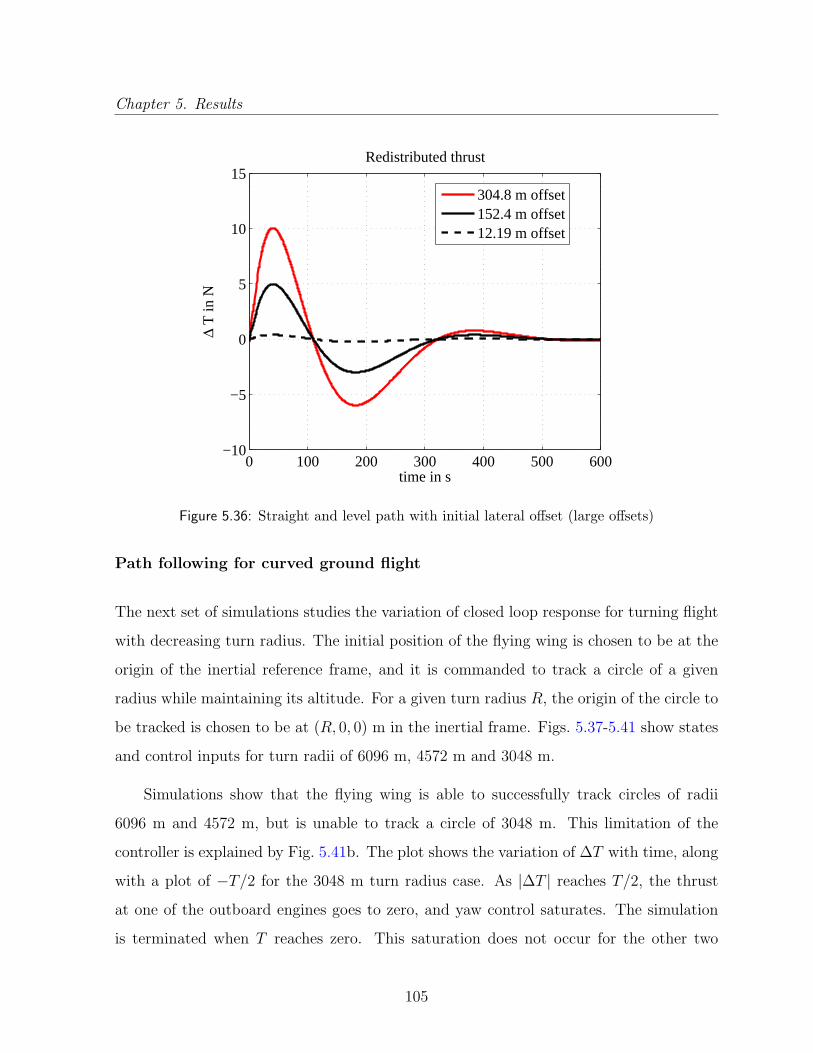
Chapter 5. Results
0 100 200 300 400 500 600−10
−5
0
5
10
15
time in s
Δ T
in N
Redistributed thrust
304.8 m offset152.4 m offset12.19 m offset
Figure 5.36: Straight and level path with initial lateral offset (large offsets)
Path following for curved ground flight
The next set of simulations studies the variation of closed loop response for turning flight
with decreasing turn radius. The initial position of the flying wing is chosen to be at the
origin of the inertial reference frame, and it is commanded to track a circle of a given
radius while maintaining its altitude. For a given turn radius R, the origin of the circle to
be tracked is chosen to be at (R, 0, 0) m in the inertial frame. Figs. 5.37-5.41 show states
and control inputs for turn radii of 6096 m, 4572 m and 3048 m.
Simulations show that the flying wing is able to successfully track circles of radii
6096 m and 4572 m, but is unable to track a circle of 3048 m. This limitation of the
controller is explained by Fig. 5.41b. The plot shows the variation of ∆T with time, along
with a plot of −T/2 for the 3048 m turn radius case. As |∆T | reaches T/2, the thrust
at one of the outboard engines goes to zero, and yaw control saturates. The simulation
is terminated when T reaches zero. This saturation does not occur for the other two
105

Chapter 5. Results
cases, and the flying wing is able to successfully follow the corresponding ground paths.
For the cases corresponding to the two larger radii, ∆R and altitude go to zero as the
transients die down, and aileron deflection, ∆T and roll angle converge to a non-zero value
corresponding to the equilibrium for turning flight.
In order to overcome the inability of the flying wing to turn with a radius of 3048 m,
the initial position of the flying wing is moved to (0,−L1, 0) m, where L1 is the lookforward
distance of the guidance law. This change in initial position tells the controller of the
circular path to be followed before the flying wing actually reaches the origin of the
inertial XY plane, which is a point on the circular path. With this change, the flying
wing is able to successfully follow a circle of radius 3048 m as seen from Figs. 5.42-5.46.
However, when the radius is decreased to 1524 m, the flying wing is no longer able to
follow the corresponding circular ground path as the yaw control saturates as seen in
Fig. 5.46b.
0 100 200 300 400 500 600−50
0
50
100
150
200
time in s
Δ R
Variation from radius of commanded path
3048 m radius4572 m radius6096 m radius
(a) ∆ R history
Figure 5.37: Curved ground path with no initial offset (small radii)
106

Chapter 5. Results
0 100 200 300 400 500 600−1
0
1
2
3
4
5
6
time in s
heig
ht in
m
altitude in m
3048 m radius4572 m radius6096 m radius
(a) Altitude history
0 100 200 300 400 500 6000
5
10
15
20
time in s
θ in
°
Pitch angle
3048 m radius4572 m radius6096 m radius
(b) Pitch angle history
Figure 5.38: Curved ground path with no initial offset (small radii)
107

Chapter 5. Results
0 100 200 300 400 500 600−8
−6
−4
−2
0
2
4
6
8
time in s
φ in
°
Roll angle
3048 m radius4572 m radius6096 m radius
(a) Roll angle history
0 100 200 300 400 500 600−100
−80
−60
−40
−20
0
20
40
time in s
ψ in
°
Yaw angle
3048 m radius4572 m radius6096 m radius
(b) Yaw angle history
Figure 5.39: Curved ground path with no initial offset (small radii)
108

Chapter 5. Results
0 100 200 300 400 500 6000
10
20
30
40
50
60
time in s
T in
N
Thrust
3048 m radius4572 m radius6096 m radius
(a) Thrust history
0 100 200 300 400 500 6000
5
10
15
20
25
time in s
flap
in °
flap deflection
3048 m radius4572 m radius6096 m radius
(b) Flap history
Figure 5.40: Curved ground path with no initial offset (small radii)
109

Chapter 5. Results
0 100 200 300 400 500 600−50
0
50
100
time in s
aile
ron
in °
aileron deflection
3048 m radius4572 m radius6096 m radius
(a) Aileron history
0 100 200 300 400 500 600−30
−20
−10
0
10
20
30
time in s
Δ T
in N
Redistributed thrust
3048 m radius+/−T/2 for 3048 m radius4572 m radius6096 m radius
(b) ∆ Thrust history
Figure 5.41: Curved ground path with no initial offset (small radii)
110

Chapter 5. Results
0 1000 2000 3000 4000 5000 6000−3000
−2000
−1000
0
1000
2000
3000
y co−ord in m
x co
−or
d in
m
ground track
flight pathcommanded 3048 m radius
(a) Ground track history
0 100 200 300 400 500 600−80
−60
−40
−20
0
20
40
60
80
time in s
Δ R
in m
Variation from radius of commanded path
3048 m radius1524 m radius
(b) ∆ R history
Figure 5.42: Curved ground path with no initial offset (guidance law activated early)
111

Chapter 5. Results
0 100 200 300 400 500 600−1
0
1
2
3
4
5
6
time in s
heig
ht in
m
altitude in m
3048 m radius1524 m radius
(a) Altitude history
0 100 200 300 400 500 6000
5
10
15
20
time in s
θ in
°
Pitch angle
3048 m radius1524 m radius
(b) Pitch angle history
Figure 5.43: Curved ground path with no initial offset (guidance law activated early)
112
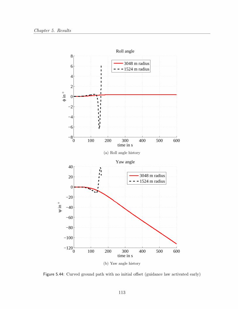
Chapter 5. Results
0 100 200 300 400 500 600−8
−6
−4
−2
0
2
4
6
8
time in s
φ in
°
Roll angle
3048 m radius1524 m radius
(a) Roll angle history
0 100 200 300 400 500 600−120
−100
−80
−60
−40
−20
0
20
40
time in s
ψ in
°
Yaw angle
3048 m radius1524 m radius
(b) Yaw angle history
Figure 5.44: Curved ground path with no initial offset (guidance law activated early)
113
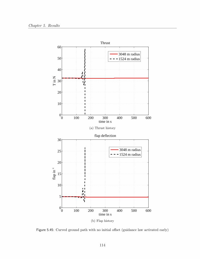
Chapter 5. Results
0 100 200 300 400 500 6000
10
20
30
40
50
60
time in s
T in
N
Thrust
3048 m radius1524 m radius
(a) Thrust history
0 100 200 300 400 500 6000
5
10
15
20
25
30
time in s
flap
in °
flap deflection
3048 m radius1524 m radius
(b) Flap history
Figure 5.45: Curved ground path with no initial offset (guidance law activated early)
114
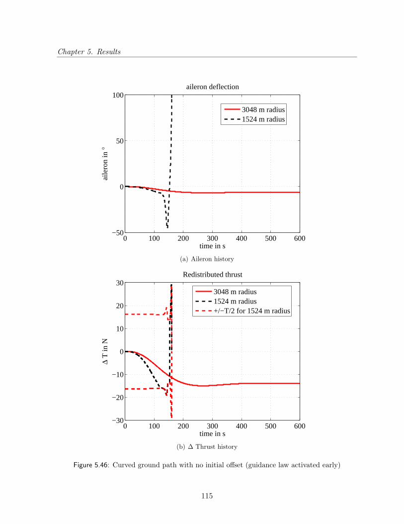
Chapter 5. Results
0 100 200 300 400 500 600−50
0
50
100
time in s
aile
ron
in °
aileron deflection
3048 m radius1524 m radius
(a) Aileron history
0 100 200 300 400 500 600−30
−20
−10
0
10
20
30
time in s
Δ T
in N
Redistributed thrust
3048 m radius1524 m radius+/−T/2 for 1524 m radius
(b) ∆ Thrust history
Figure 5.46: Curved ground path with no initial offset (guidance law activated early)
115

Chapter 5. Results
5.3.4 Path-following with abrupt change in payload mass
This set of simulations involves an abrupt change in the payload mass carried by the
flexible flying wing. The airplane is trimmed in straight and level flight at 12.19 m/s at
the origin of the inertial reference frame with the velocity vector along the inertial Y axis
and is commanded to maintain its heading and altitude. The initial payload at the center
of the flying wing is set as 181.4 kg (corresponding to the ‘heavy’ case). At t = 50 s,
the payload is decreased abruptly. The three cases considered correspond to a decrease
in payload by 50% and 25% respectively and are plotted in Figs. 5.47-5.49.
The change in payload mass also results in an abrupt change in the equilibrium aeroe-
lastic state vector. Simulations show that the controller is able to control the transients
due to the abrupt change in payload mass and drive the states to the new equilibrium
condition. The change in payload mass causes the altitude to increase initially due a drop
in the mass of the airplane as shown in Fig. 5.47b. The altitude of the airplane then
decreases before coming back to its initial value. Once again, the transient flap response
exhibits high frequency oscillations due to coupling with bending modes. The magnitude
of the transient response is shown to increase with an increase in the change in the payload
mass.
116

Chapter 5. Results
0 100 200 300 400 500 600−40
−30
−20
−10
0
10
time in s
heig
ht in
m
altitude in m
50 % decrease25 % decrease
(a) Altitude history
40 45 50 55 60−0.2
−0.15
−0.1
−0.05
0
0.05
0.1
0.15
0.2
time in s
heig
ht in
m
altitude in m
50 % decrease25 % decrease
(b) Altitude history showing detail at t = 50s
Figure 5.47: Path following with abrupt change in payload mass
117

Chapter 5. Results
0 100 200 300 400 500 60020
30
40
50
60
70
80
time in s
T in
N
Thrust
50 % decrease25 % decrease
(a) Thrust history
0 100 200 300 400 500 6004.5
5
5.5
6
6.5
7
7.5
8
time in s
flap
in °
flap deflection
50 % decrease25 % decrease
(b) Flap history
Figure 5.48: Path following with abrupt change in payload mass
118

Chapter 5. Results
0 100 200 300 400 500 600−8
−6
−4
−2
0
2
4
6
time in s
θ in
°
Pitch angle
50 % decrease25 % decrease
(a) Pitch angle history
Figure 5.49: Path following with abrupt change in payload mass
5.3.5 Dependence of computational time on discretization
Fig. 5.50 plots the variation of the log of the computational time in hours versus the log of
the number of nodes on the flying wing. The number of nodes used in the simulation are
19, 25, 31, 37 and 43. The flying wing is commanded to maintain its heading and increase
its altitude by 12.19 m. 30 s of flying time is simulated, which for a time-step of 0.02 s,
corresponds to 1500 iterations. The simulations are carried out using MATLAB 7.6.0.324
on a Intel R© CoreTM2 Quad CPU Q 9550 with 4 GB RAM and 32-bit Windows XP. The
slope of the graph has a value of 1.3, which implies that the dependence of computational
time on the number of nodes is close to linear.
119

Chapter 5. Results
2.8 3 3.2 3.4 3.6 3.80.4
0.6
0.8
1
1.2
1.4
1.6
1.8
2
log of number of nodes
log
of ti
me
in h
rs
Computational time dependence on nodes
Figure 5.50: Variation of computational time with number of nodes
120
Chapter 6
Conclusions and Future Work
6.1 Conclusions
The objectives of this dissertation were to study the unique flight dynamic characteristics
of flexible, high aspect-ratio flying wings and to design a flight control law for path-
following. The flight dynamics was studied using an integrated model of the aeroelasticity
and flight dynamics of flexible high aspect ratio flying wings developed by Patil and
Hodges [7]. This includes analysis of lateral dynamics which was not studied by Patil and
Hodges. It was found that a rigid body model that accounted for the static aeroelastic
deformation at trim captured the predominant flight dynamic characteristics shown by
the flexible flying wing. Moreover, this rigid body model was found to predict the onset
of dynamic instability in the flight dynamics seen in the integrated model. A modified
criteria was introduced for predicting the onset of static instability in the presence of large
aeroelastic deformation.
Using the concept of the mean axis, a six degree-of-freedom reduced order model of
the flight dynamics is constructed that minimizes the coupling between rigid body modes
and the structural dynamics while accounting for the static aeroelastic deformation of
121

Chapter 6. Conclusions and Future Work
the flying wing. The original derivation of the equations of motion for a deformable
airplane by Milne assumed small deformations [9]. This assumption is not made in the
equations derived in this dissertation. Multi-step nonlinear dynamic inversion applied
to this reduced order model is coupled with a nonlinear guidance law to design a flight
controller for path following. The controls computed by this flight controller are used as
inputs to a time-marching simulation of the integrated model of aeroelasticity and flight
dynamics. Simulation results presented in this dissertation show that the controller is
able to successfully follow both straight line and curved ground paths while maintaining
the desired altitude. The controller is also shown to be able to handle an abrupt change
in payload mass while path-following.
Finally, the equations of motion of the integrated model were non-dimensionalized
to identify aeroelastic parameters for optimization and design of high aspect-ratio flying
wings.
6.2 Future Work
Though the concept of a controller for a flexible, high aspect-ratio flying wing has been
proven in this dissertation, further work needs to be done before this system can be
implemented on an actual airplane. Some of the questions that need to be addressed are
listed below:
• The aeroelastic model used for linear stability analysis and time-marching simulation
needs to be validated with experimental data. This data is not publicly available at
this point in time.
• The controller used in this dissertation takes the velocities and angular velocities
of nodes from the simulation as inputs for computing mean axis parameters. In a
real system, these quantities will have to be estimated as shown in Section 4.6. The
122

Chapter 6. Conclusions and Future Work
effect of this state estimation on the closed loop system needs to be addressed.
• The controller needs to be augmented for gust load alleviation and its effect on the
complete closed-loop system needs to be studied.
• Actuator dynamics are not modeled in this dissertation, and the effect of these
dynamics on both the aeroelasticity and flight dynamics needs to be studied.
• The configuration used to study open loop dynamics was found to be subject to
control reversal. This was overcome by increasing the torsional rigidity of the con-
figuration for closed loop simulations. However, the effect of static aeroelasticity
on the effectiveness of tailing edge control surfaces and its implications for flight
control needs to be studied in detail and accounted for in control design.
• The controller design implemented in this dissertation assumes that model used by
the controller is known exactly. As this will not be the case in a real system, the
robustness of the controller with respect to uncertainties in the model needs to be
studied.
123

Bibliography
[1] “NASA - NASA Dryden Fact Sheet - Solar-Power Research,”
http://www.nasa.gov/centers/dryden/news/FactSheets/FS-054-DFRC.html.
[2] Noll, T. E., Brown, J. M., Perez-Davis, M. E., Ishmael, S. D., Tiffany, G. E.,
and Gaier, M., “Investigation of the Helios Prototype Aircraft Mishap,” Tech. rep.,
NASA, 2004.
[3] DARPA, “Vulture Program: Broad Agency Announcement Solicitation 07-51,” July
2007.
[4] “DARPA-Vulture Program,” http://www.darpa.mil/news images/vulture-01.html.
[5] “DARPA-Vulture Program,” http://www.darpa.mil/news images/vulture-02.html.
[6] “DARPA-Vulture Program,” http://www.darpa.mil/news images/vulture-03.html.
[7] Patil, M. J. and Hodges, D. H., “Flight Dynamics of Highly Flexible Flying Wings,”
Journal of Aircraft , Vol. 43, No. 6, Nov. – Dec. 2006, pp. 1790 – 1798.
[8] Skoog, R. B., “An Analysis of the Effects of Aeroelasticity on Static Longitudinal
Stability and Control of a Swept Wing Airplane,” Tech. Rep. 1298, NACA, Jan.
1957.
[9] Milne, R. D., “Dynamcis of the Deformable Aeroplane,” R&M 3345, British Aero-
nautical Research Council, 1964.
124

BIBLIOGRAPHY
[10] Milne, R. D., “Some Remarks on the Dynamcis of Deformable Bodies,” AIAA Jour-
nal , Vol. 6, No. 3, Mar. 1968, pp. 556 – 558.
[11] Wykes, J. H. and Lawrence, R. E., “Aerothermoelasticity: Its Impact on Stability
and Control of Winged Aerospace Vehicles,” Journal of Aircraft , Vol. 2, No. 6, Nov.
– Dec. 1965, pp. 517 – 526.
[12] Rodden, W. P., “Dihedral Effect of a Flexible Wing,” Journal of Aircraft , Vol. 2,
No. 5, Sep. – Oct. 1965, pp. 368 – 373.
[13] Swaim, R. L. and Fullman, D. G., “Prediction of Elastic-Airplane Longitudinal Dy-
namics from Rigid-Body Aerodynamics,” Journal of Aircraft , Vol. 14, No. 9, Sep.
1977, pp. 868 – 873.
[14] Swaim, R. L. and Staab, G. H., “Prediction of Elastic-Airplane Lateral Dynamics
from Rigid-Body Aerodynamics,” Journal of Aircraft , Vol. 15, No. 7, Jul. 1978,
pp. 392 – 398.
[15] Weisshaar, T. A. and Ashley, H., “Static Aeroelasticity and the Flying Wing,” Jour-
nal of Aircraft , Vol. 10, No. 10, Oct. 1973, pp. 586 – 594.
[16] Weisshaar, T. A. and Ashley, H., “Static Aeroelasticity and the Flying Wing, Revis-
ited,” Journal of Aircraft , Vol. 11, No. 11, Nov. 1974, pp. 718 – 720.
[17] Rodden, W. P. and Love, J. R., “Equations of Motion of a Quasisteady Flight Vehicle
Utilizing Restrained Static Aeroelastic Characteristics,” Journal of Aircraft , Vol. 22,
No. 9, Sep. 1985, pp. 802 – 809.
[18] Dykman, J. R. and Rodden, W. P., “Structural Dynamics and Quasistatic Aeroelastic
Equations of Motion,” Journal of Aircraft , Vol. 37, No. 3, May – Jun. 2000, pp. 538
– 542.
[19] Karpel, M., “Reduced-Order Aeroelastic Models via Dynamic Residualization,” Jour-
nal of Aircraft , Vol. 27, No. 5, May 1990, pp. 449 – 455.
125

BIBLIOGRAPHY
[20] Waszak, M. R. and Schmidt, D. K., “Flight Dynamics of Aeroelastic Vehicles,” Jour-
nal of Aircraft , Vol. 25, No. 6, Jun. 1988, pp. 563 – 571.
[21] Schmidt, D. K. and Raney, D. L., “Modeling and Simulation of Flexible Flight Vehi-
cles,” Journal of Guidance, Control and Dynamics , Vol. 24, No. 3, May – Jun. 2001,
pp. 539 – 546.
[22] Newman, B. and Schmidt, D. K., “Numerical and Literal Aeroelastic-Vehicle-Model
Reduction for Feedback Control Synthesis,” Journal of Guidance, Control and Dy-
namics , Vol. 14, No. 5, Sep. – Oct. 1991, pp. 943 – 953.
[23] Livneh, R. and Schmidt, D. K., “Unified Literal Approximations for Longitudinal
Dynamics of Flexible Flight Vehicles,” Journal of Guidance, Control and Dynamics ,
Vol. 18, No. 5, Sep. – Oct. 1995, pp. 1074 – 1083.
[24] Siepenkotter, A. and Alles, W., “Stability analysis of the nonlinear dynamics of
flexible aircraft,” Aerospace Science and Technology , Vol. 9, No. 2, Mar. 2005, pp. 135
– 141.
[25] Buttrill, C. S., Zeiler, T. A., and Arbuckle, P. D., “Nonlinear Simulation of a Flex-
ible Aircraft in Maneuvering Flight,” Proceedings of the AIAA Flight Simulation
Technologies Conference, Monterey, CA, August 1987, AIAA-1987-2501.
[26] Drela, M., “Integrated Simulation Model for Preliminary Aerodynamic,
Structural, and Control-law Design of Aircraft,” Proceedings of the 40th
AIAA/ASME/ASCE/AHS/ASC Structures, Structural Dynamics, and Materials
Conference, St. Louis, MO, April 1999, AIAA-1999-1394.
[27] Winther, B. A., Goggin, P. J., and Dykman, J. R., “Reduced-Order Dynamic Aeroe-
lastic Model Development and Integration with Nonlinear Simulation,” Journal of
Aircraft , Vol. 37, No. 5, Sep. – Oct. 2000, pp. 833 – 839.
126

BIBLIOGRAPHY
[28] Reschke, C., Integrated Flight Loads Modelling and Analysis for Flexible Transport
Aircraft , Ph.D. thesis, University of Stuttgart, Sturrgart, Germany, July 2006.
[29] Nguyen, N., “Integrated Flight Dynamic Modeling of Flexible Aircraft with Inertial
Force-Propulsion-Aeroelastic Coupling,” Proceedings of the 46th AIAA Aerospace
Sciences Meeting and Exhibit , Reno, NV, January 2008, AIAA-2008-194.
[30] Freymann, R., “Dynamic Interactions between Active Control Systems and a Flexible
Aircraft Structure,” Proceedings of the 27th Structures, Structural Dynamics and
Materials Conference, San Antonio, TX, May 1986, AIAA-1986-0960.
[31] Kubica, F., Livet, T., Le Tron, X., and Bucharles, A., “Parameter-Robust Flight
Control System for a Flexible Aircraft,” Control Engineering Practice, Vol. 3, No. 9,
Sep. 1995, pp. 1209 – 1215.
[32] Becker, J., Caldwell, B., and Vaccaro, V., “The Interaction of Flight Control Sys-
tem and Aircraft Structure,” Proceedings of the RTO AVT Specialists’ Meeting on
’Structural Aspects of Flexible Aircraft Control’ , Ottawa, Cananda, October 1999, 4.
[33] van Etten, C., Balas, G. J., and Bennani, S., “Linear Parametrically Varying In-
tegrated Flight and Structural Mode Control for a Flexible Aircraft,” Proceedings
of the AIAA Guidance, Navigation, and Control Conference and Exhibit , Portland,
OR, August 1999, AIAA-1999-4217.
[34] Miyazawa, Y., “Flight Control Law and Structural Filter Design for a Flexible
Aerospace Vehicle,” Proceedings of the AIAA Guidance, Navigation, and Control
Conference and Exhibit , Denver, CO, August 2000, AIAA-2000-4256.
[35] Alazard, D., “Robust H2 Design for Lateral Flight Control of Highly Flexible Air-
craft,” Journal of Guidance, Control and Dynamics , Vol. 25, No. 3, May – Jun. 2002,
pp. 502 – 509.
127
BIBLIOGRAPHY
[36] Goman, M., Sidoryuk, M., and Ustinov, A., “Control Law Design for Flexible Air-
craft: Comparison of the H∞-based and Classical Methods,” Proceedings of the AIAA
Guidance, Navigation, and Control Conference and Exhibit , San Francisco, CA, Au-
gust 2005, AIAA-2005-6265.
[37] Silvestre, F. and Paglione, P., “Dynamics and Control of a Flexible Aircraft,” Proceed-
ings of the AIAA Atmospheric Flight Mechanics Conference and Exhibit , Honolulu,
HI, August 2008, AIAA-2008-6876.
[38] Gregory, I. M., “Dynamic Inversion to Control Large Flexible Aircraft,” Proceedings
of the AIAA Guidance, Navigation, and Control Conference and Exhibit , Boston,
MA, 1998, AIAA-1998-4323.
[39] Gregory, I. M., “Modified Dynamic Inversion to Control Large Flexible Aircraft -
What’s Going On?” Proceedings of the AIAA Guidance, Navigation, and Control
Conference and Exhibit , Portland, OR, 1999, AIAA-1999-3998.
[40] Gregory, I. M., “Stability Result for Dynamic Inversion Devised to Control Large
Flexible Aircraft,” Proceedings of the AIAA Guidance, Navigation, and Control Con-
ference and Exhibit , Montreal, Canada, August 2001, AIAA-2001-4284.
[41] Meirovitch, L. and Tuzcu, I., “Unified Theory for the Dynamics and Control of
Maneuvering Flexible Aircraft,” AIAA Journal , Vol. 42, No. 4, Apr. 2004, pp. 714 –
727.
[42] Meirovitch, L. and Tuzcu, I., “Time Simulations of the Response of Maneuvering
Flexible Aircraft,” Journal of Guidance, Control and Dynamics , Vol. 27, No. 5, Sep.
– Oct. 2004, pp. 814 – 828.
[43] Tuzcu, I. and Meirovitch, L., “Effects of Flexibility on the Stability of Flying Air-
craft,” Journal of Dynamic Systems, Measurement, and Control , Vol. 127, No. 1,
Mar. 2005, pp. 41 – 49.
128
BIBLIOGRAPHY
[44] Meirovitch, L. and Tuzcu, I., “Control of Flexible Aircraft Executing Time-
Dependent Maneuvers,” Journal of Guidance, Control and Dynamics , Vol. 28, No. 6,
Nov. – Dec. 2005, pp. 1291 – 1300.
[45] Patil, M. J., Hodges, D. H., and Cesnik, C. E. S., “Characterizing the Effects of
Geometrical Nonlinearities on Aeroelastic Behavior of High-Aspect-Ratio Wings,”
Proceedings of the International Forum on Aeroelasticity and Structural Dynamics ,
Williamsburg, VA, June 1999.
[46] Frulla, G., “Aeroelastic behaviour of a solar-powered high-altitude long endurance
unmanned air vehicle (UAV) slender wing,” Proceedings of the I MECH E Part G
Journal of Aerospace Engineering , Vol. 218, No. 3, 2004, pp. 179 – 188.
[47] Patil, M. J. and Hodges, D. H., “On the importance of aerodynamic and structural
geometrical nonlinearities in aeroelastic behavior of high-aspect-ratio wings,” Journal
of Fluids and Structures , Vol. 19, No. 7, Aug. 2004, pp. 905 – 915.
[48] Patil, M. J., Hodges, D. H., and Cesnik, C. E. S., “Nonlinear Aeroelastic Ananlysis
of Complete Aircraft in Subsonic Flow,” Journal of Aircraft , Vol. 37, No. 5, Sep. –
Oct. 2000, pp. 753 – 760.
[49] Patil, M. J., Hodges, D. H., and Cesnik, C. E. S., “Limit-Cycle Oscillations in High-
Aspect-Ratio Wings,” Journal of Fluids and Structures , Vol. 15, No. 1, Jan. 2001,
pp. 107 – 132.
[50] Tang, D. and Dowell, E. H., “Effects of geometric structural nonlinearity on flut-
ter and limit cycle oscillations of high-aspect-ratio wings,” Journal of Fluids and
Structures , Vol. 19, No. 3, Apr. 2004, pp. 291 – 306.
[51] Tang, D. and Dowell, E. H., “Experimental and Theoretical Study on Aeroelastic
Response for High-Aspect-Ratio Wing,” AIAA Journal , Vol. 39, No. 8, Aug. 2001,
pp. 1430 – 1441.
129
BIBLIOGRAPHY
[52] Tang, D. and Dowell, E. H., “Limit-Cycle Hysteresis Response for a High-Aspect-
Ratio Wing Model,” Journal of Aircraft , Vol. 39, No. 5, Sep. – Oct. 2002, pp. 885 –
888.
[53] Romeo, G., Frulla, G., Cestino, E., Marzocca, P., and Tuzcu, I., “Non-Linear
Aeroelastic Modeling and Experiments of Flexible Wings,” Proceedings of the 47th
AIAA/ASME/ASCE/AHS/ASC Structures, Structural Dynamics, and Materials
Conference, Newport, RI, May 2006, AIAA-2006-2186.
[54] Patil, M. J. and Hodges, D. H., “Output Feedback Control of the Nonlinear Aeroe-
lastic Response of a Slender Wing,” Journal of Guidance, Control and Dynamics ,
Vol. 25, No. 2, Mar. – Apr. 2002, pp. 302 – 308.
[55] Cesnik, C. E. S. and Brown, E. L., “Modeling of High Aspect Ratio Active Flexible
Wings for Roll Control,” Proceedings of the 43rd AIAA/ASME/ASCE/AHS/ASC
Structures, Structural Dynamics, and Materials Conference, Denver, CO, April 2002,
AIAA-2002-1719.
[56] Su, W. and Cesnik, C. E. S., “Nonlinear Aeroelastic Modeling and Analysis of
Fully Flexible Aircraft,” Proceedings of the 46th AIAA/ASME/ASCE/AHS/ASC
Structures, Structural Dynamics, and Materials Conference, Austin, TX, April 2005,
AIAA-2005-2169.
[57] Smith, M. J., Patil, M. J., and Hodges, D. H., “CFD-Based Analysis of Nonlin-
ear Aeroelastic Behavior of High-Aspect-Ratio Wings,” Proceedings of the 42nd
AIAA/ASME/ASCE/AHS/ASC Structures, Structural Dynamics, and Materials
Conference, Seattle, WA, April 2001, AIAA-2001-1582.
[58] Palacios, R. and Cesnik, C. E. S., “Static Nonlinear Aeroelasticity of
Flexible Slender Wings in Compressible Flow,” Proceedings of the 46th
AIAA/ASME/ASCE/AHS/ASC Structures, Structural Dynamics, and Materials
Conference, Austin, TX, April 2005, AIAA-2005-1945.
130
BIBLIOGRAPHY
[59] Garcia, J. A., “Numerical Investigation of Nonlinear Aeroelastic Effects on Flexible
High-Aspect-Ratio Wings,” Journal of Aircraft , Vol. 42, No. 4, July – Aug. 2005,
pp. 1025 – 1036.
[60] Vartio, E., Shimko, A., Tilmann, C. P., and Flick, P. M., “Structural Modal Con-
trol and Gust Load Alleviation for a SensorCraft Concept,” Proceedings of the
46th AIAA/ASME/ASCE/AHS/ASC Structures, Structural Dynamics, and Mate-
rials Conference, Austin, TX, April 2005, AIAA-2005-1946.
[61] Vartio, E., Shaw, E., and Vetter, T., “Gust Load Alleviation Flight Control System
Design fir a SensorCraft Vehicle,” Proceedings of the 26th AIAA Applied Aerodynamic
Conference, Honolulu, HI, August 2008, AIAA-2008-7192.
[62] Penning, K., Zink, P., Wei, P., De La Garza, A., Love, M., and Martinez, J., “GLA
and Flutter Suppression for a SensorCraft Class Concept Using System Identifica-
tion,” Proceedings of the 26th AIAA Applied Aerodynamics Conference, Honolulu,
HI, August 2008, AIAA-2008-7188.
[63] Gregory, I. M., Cao, C., Patel, V. V., and Hovakimyan, N., “Adaptive Control Laws
for Flexible Semi-Span Wind Tunnel Model of High-Aspect Ratio Flying Wing,”
Proceedings of the AIAA Guidance, Navigation, and Control Conference and Exhibit ,
Hilton Head, SC, August 2007, AIAA-2007-6525.
[64] Banerjee, J. R., “Flutter Characteristics of High Aspect Ratio Tailless Aircraft,”
Journal of Aircraft , Vol. 21, No. 9, Sep. 1984, pp. 733 – 736.
[65] Banerjee, J. R., “Flutter Modes of High Aspect Ratio Tailless Aircraft,” Journal of
Aircraft , Vol. 25, No. 5, May 1988, pp. 473 – 476.
[66] Banerjee, J. R. and Cal, A. A., “A Unified Approach to Stability Characteristics of
Tailless Aircraft,” In Proceedings of the 29th Structures, Structural Dynamics and
Materials Conference, Williamsburg, VA, Apr. 1988, AIAA-1988-2212.
131
BIBLIOGRAPHY
[67] Zerweckh, S. H., von Flotow, A. H., and Murray, J. E., “Flight Testing a Highly
Flexible Aircraft: Case Study on the MIT Light Eagle,” Journal of Aircraft , Vol. 27,
No. 4, Apr. 1990, pp. 342 – 349.
[68] van Schoor, M. C. and von Flotow, A. H., “Aeroelastic Characteristics of a Highly
Flexible Aircraft,” Journal of Aircraft , Vol. 27, No. 10, Oct. 1990, pp. 901 – 908.
[69] Patil, M. J., Hodges, D. H., and Cesnik, C. E. S., “Nonlinear Aeroelasticity and
Flight Dynamics of High-Altitude Long-Endurance Aircraft,” Journal of Aircraft ,
Vol. 38, No. 1, Jan. – Feb. 2001, pp. 88 – 94.
[70] Patil, M. J., Hodges, D. H., and Cesnik, C. E. S., “Limit Cycle Oscillations of a
Complete Aircraft,” Proceedings of the 41th AIAA/ASME/ASCE/AHS/ASC Struc-
tures, Structural Dynamics, and Materials Conference, Atlanta, GA, April 2000,
AIAA-2000-1395.
[71] Su, W. and Cesnik, C. E. S., “Dynamic Response of Highly Flexible Flying Wings,”
Proceedings of the 47th AIAA/ASME/ASCE/AHS/ASC Structures, Structural Dy-
namics, and Materials Conference, Newport, RI, May 2006, AIAA-2006-1636.
[72] Chang, C.-S., Hodges, D. H., and Patil, M. J., “Aeroelastic Characteristics of a
Highly Flexible Aircraft,” Journal of Aircraft , Vol. 45, No. 2, Mar. - Apr. 2008,
pp. 538 – 545.
[73] Shearer, C. M. and Cesnik, C. E. S., “Nonlinear Flight Dynamics of Very Flexible
Aircraft,” Journal of Aircraft , Vol. 44, No. 5, Sep. – Oct. 2007, pp. 1528 – 1545.
[74] Shearer, C. M. and Cesnik, C. E. S., “Trajectory Control for Very Flexible Aircraft,”
Journal of Guidance, Control and Dynamics , Vol. 31, No. 2, Mar. – Apr. 2008,
pp. 340 – 357.
[75] Love, M. H., Zink, P. S., Wieselmann, P. A., and Youngren, H., “Body Free-
dom Flutter of High Aspect Ratio Flying Wings,” Proceedings of the 46th
132

BIBLIOGRAPHY
AIAA/ASME/ASCE/AHS/ASC Structures, Structural Dynamics, and Materials
Conference, Austin, TX, April 2005, AIAA-2005-1947.
[76] Tuzcu, I., Marzocca, P., Cestino, E., Romeo, G., and Frulla, G., “Stability and
Control of a High-Altitude, Long-Endurance UAV,” Journal of Guidance, Control,
and Dynamics , Vol. 30, No. 3, May – June 2007, pp. 713 – 721.
[77] Hodges, D. H., “A Mixed Variational Formulation Based on Exact Intrinsic Eequa-
tions for Dynamics of Moving Beams,” Int. Journal of Solids and Structures , Vol. 26,
No. 11, Nov. 1990, pp. 1253 – 1273.
[78] Hodges, D. H., “Geometrically Exact, Intrinsic Theory for Dynamics of Curved and
Twisted Anisotropic Beams,” AIAA Journal , Vol. 41, No. 6, June 2003, pp. 1131 –
1137.
[79] Peters, D. A. and Johnson, M. J., “Finite-State Airloads for Deformable Airfoils on
Fixed and Rotating Wings,” Proceedings of the Winter Annual Meeting, Symposium
on Aeroelasiticity and Fluid/Structure Interaction, Fairfield, NJ, 1994, American
Socity of Mechanical Engineers.
[80] Peters, D. A., Karunamoorthy, S., and Cao, W.-M., “Finite State Induced Flow
Models, Part I: Two-Dimensional Thin Airfoil,” Journal of Aircraft , Vol. 32, No. 2,
Mar. – Apr. 1995, pp. 313 – 322.
[81] Meirovitch, L., Fundamentals of Vibrations , McGraw Hill, 2001, p. 385.
[82] Wolowicz, C. H., Bowman Jr., J. S., and Gilbert, W. P., “Similitude Requirements
and Scaling Relationships as Applied to Model Testing,” Tech. Rep. Technical Paper
1435, NASA, 1979.
[83] Park, S., Deyst, J., and How, J. P., “Performance and Lyapunov Stability of a Nonlin-
ear Path-Following Guidance Method,” Journal of Guidance, Control and Dynamics ,
Vol. 30, No. 6, Nov. – Dec. 2007, pp. 1718 – 1728.
133

BIBLIOGRAPHY
[84] Bugajski, D. J. and Enns, D. F., “Nonlinear Control Law with Application to High
Angle-of-Attack Flight,” Journal of Guidance, Control and Dynamics , Vol. 15, No. 3,
May – Jun. 1992, pp. 761 – 767.
[85] Snell, S. A., Enns, D. F., and Garrard Jr., W. L., “Nonlinear Inversion Flight Control
for a Supermaneuverable Aircraft,” Journal of Guidance, Control and Dynamics ,
Vol. 15, No. 4, July – Aug. 1992, pp. 976 – 984.
[86] Enns, D. F., Bugajski, D. J., Hendrick, R., and Stein, G., “Dynamic inversion: an
evolving methodology for flight control design,” International Journal of Control ,
Vol. 59, No. 1, Jan 1994, pp. 71 – 91.
[87] Stevens, B. L. and Lewis, F. L., Aircraft Control and Simulation, John Wiley & Sons,
New Jersey, 2nd ed., 2003.
[88] Ito, D., Georgie, J., Valasek, J., and Ward, D. T., “Reentry Vehicle Flight Con-
trols Design Guidelines: Dynamic Inversion,” NASA TP 2002-210771, Texas A&M
University, 2002.
[89] Cotting, M. C. and Cox, T. M., “A Generic Guidance and Control Structure for
Six-Degree-of-Freedom Conceptual Aircraft Design,” Proceedings of the 43rd AIAA
Aerospace Sciences Meeting and Exhibit , Reno, NV, January 2005, AIAA-2005-0032.
[90] Goland, M., “The Flutter of a Uniform Cantilever Wing,” Journal of Applied Me-
chanics , Vol. 12, No. 4, 1945, pp. A197–A208.
[91] Goland, M. and Luke, Y., “The Flutter of a Uniform Cantilever Wing with Tip
Weights,” Journal of Applied Mechanics , Vol. 15, No. 1, 1948, pp. 13–20.
[92] Anderson Jr., J. D., Aircraft Performance and Design, McGraw Hill, 1999, p. 265.
134