dynamic response of highly flexible flying wings

Dynamic Response of Highly Flexible Flying Wings

Weihua Su* and Carlos E. S. Cesnik†

The University of Michigan, Ann Arbor, MI, 48109-2140

This paper presents a method to model the coupled nonlinear flight dynamics and aeroelasticity of highly flexible flying wings, as well as analyze their nonlinear characteristics. A low-order, nonlinear, strain-based finite element framework is used, which is capable of assessing the fundamental impact of structural nonlinear effects in a computationally effective formulation target for preliminary vehicle design and control synthesis. The cross-sectional stiffness and inertia properties of the wings are calculated along the wing span, and then incorporated into the 1-D nonlinear beam model. A proposed model for the effects in the torsional stiffness of skin wrinkling due to large bending curvature of the wing is also presented. Finite-state unsteady subsonic aerodynamic loads are incorporated to complete the aeroelastic representation of a flying wing. In studying flying wing dynamic response, a spatially-distributed discrete gust model is introduced and its impact on the time-domain solutions is investigated.

I. Introduction LYING wings, including all-wing and tailless aircraft, belong to the concept of All Lifting Vehicles (ALV). Its history can be traced back to the work of Penaud in 1860-1870s. The development of flying wings was inspired

by the imitation of nature. After more than one hundred years of developing, flying wings are still considered as unconventional aircraft concepts. Wood and Bauer1 gave a comprehensive review on the history and development of flying wings and flying fuselages in Europe and the United States.

F Northrop made important contributions2 to the development of flying wings in the United States. His first flying

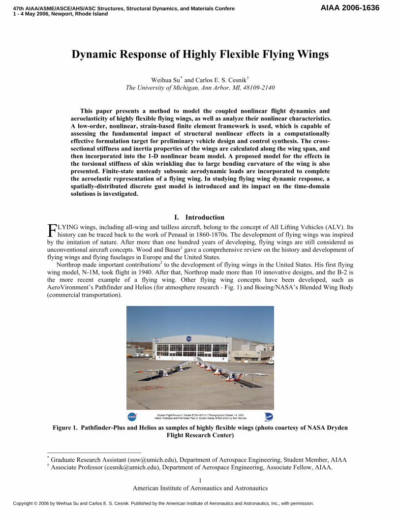
wing model, N-1M, took flight in 1940. After that, Northrop made more than 10 innovative designs, and the B-2 is the more recent example of a flying wing. Other flying wing concepts have been developed, such as AeroVironment’s Pathfinder and Helios (for atmosphere research - Fig. 1) and Boeing/NASA’s Blended Wing Body (commercial transportation).

Figure 1. Pathfinder-Plus and Helios as samples of highly flexible wings (photo courtesy of NASA Dryden

Flight Research Center)

* Graduate Research Assistant ([email protected]), Department of Aerospace Engineering, Student Member, AIAA † Associate Professor ([email protected]), Department of Aerospace Engineering, Associate Fellow, AIAA.

American Institute of Aeronautics and Astronautics

1

47th AIAA/ASME/ASCE/AHS/ASC Structures, Structural Dynamics, and Materials Confere1 - 4 May 2006, Newport, Rhode Island

AIAA 2006-1636

Copyright © 2006 by Weihua Su and Carlos E. S. Cesnik. Published by the American Institute of Aeronautics and Astronautics, Inc., with permission.

Many researchers have addressed particular issues on analysis and design of flying wings. Weisshaar and Ashley3 studied the static aeroelasticity of flying wings, including instabilities such as divergence and large twist and bending that may lead to loss of control effectiveness. Fremaux, Vairo and Whipple4 have identified some of the parameters that cause a flying wing configuration to be capable of a sustaining tumbling motion through the use of dynamically scaled generic models. In their work, effects due to the change of mass distribution and wing swept angle were presented. Esteban5 and his co-workers have performed the static and dynamic analysis of a flying wing. They concluded that by selecting the correct winglet parameters: leading edge sweep, taper ratio, winglet area, effective moment arm, and vertical coordinate of the mean aerodynamic center of the winglet, a flying wing vehicle can be constructed so that the desired lateral stability characteristics can be achieved. Mialon et al.6 performed aerodynamic optimization of subsonic flying wing configurations. In their work, CFD codes developed in ONERA were used for the analysis. Manual modifications and numerical optimization were both used during their design process. They also designed a new family of airfoils, which was better suited for their specific flying wing vehicle. The importance of geometrical parameters, such as sweep angle at leading edge, aspect ratio or shape of the generated airfoils was investigated as well. Sevant, Bloor and Wilson7 also performed the design of a subsonic flying wing, aiming at maximum lift. Response surface method was applied to solve the problem caused by the local minima, since the optimization problem is quite complex.

Like the Pathfinder-Plus and Helios shown in Fig. 1, the flying wing to be studied in this paper is a highly flexible aircraft. Highly flexible flying wings have been considered an important concept for high-altitude long-endurance unmanned aerial vehicles (HALE UAV). HALE vehicles feature light wings with high aspect ratio. These long and slender wings, by their inherent nature, can maximize lift to drag ratio. On the other hand, they may undergo large deformations during normal operating loads, exhibiting geometrically nonlinear behavior. Due to this inherently high flexibility, traditional linear theories do not provide accurate estimations on HALE’s aeroelastic characters. Patil, Hodges, and Cesnik8 studied the aeroelasticity and flight dynamics of HALE aircraft. The results indicate the aeroelastic behavior and flight dynamics characteristic of the aircraft can be significantly changed due to the large deflection of the flexible wings. van Schoor, Zerweckh and von Flotow9 studied linearized aeroelastic characteristics and control of highly flexible aircraft. They used linearized modes including rigid-body modes to predict the stability of the aircraft under different flight conditions. Their results indicate that unsteady aerodynamics and flexibility of the aircraft should be considered so as to correctly model the dynamic system. This leads to the conclusion that the coupled effects between these large deflection and vehicle flexibility and flight dynamics as well as other aeroelastic effects (e.g., gust response, flutter instability) must be properly accounted for in a nonlinear aeroelastic framework. Drela10 modeled a complete flexible aircraft as an assemblage of joined nonlinear beams. In his work, the aerodynamic model is a vortex/source-lattice with wind-aligned trailing vorticity and Prandtl-Glauert compressibility correction. The nonlinear equation was solved by using a full Newton method. Through simplifications of the model, the computational size was reduced for iterative preliminary design.

It is well known that the deformation of highly flexible flying wing vehicles is dependent on both the mission profile and operating conditions. Under certain operating conditions, the aircraft deformed shape can be significantly different from its undeformed one. In this case, the aeroelastic analysis must be based on the actual trimmed conditions.

For long slender wings, their natural frequencies are low enough that their flexible modes could interact with the body motions, such as plunging and pitching. Love et al.11 studied the body freedom flutter of a high aspect ratio flying wing model. Their results indicate that the body freedom flutter is an issue over lower altitude portions of the flight envelop and that active flutter suppression should be considered.

In 1994, NASA and industry initiated the Environmental Research Aircraft and Sensor Technology (ERAST) program aimed at developing UAV capabilities for long duration and very high altitude flights. AeroVironment’s Helios aircraft, which was a type of a very flexible flying wing aircraft, was one of the several UAVs developed under the NASA ERAST program. The mishap of the Helios prototype (HP3)12 indicates that these long, slender flying wing vehicles can be very sensitive to disturbance. The large deformation with a high dihedral angle gives the vehicle a severe operating condition, particularly under gust conditions.

Gusts are random in nature. They can affect different aspects of the aircraft’s operation, such as its dynamic loads, flight stability and safety, and controls.13 In a high-fidelity analysis, a random gust is represented by a continuous model. However, discrete gust models are still used due to its simplicity (including being part of commercial aircraft certification regulations). The main difference between the continuous and discrete gust analysis is that the former is statistical while the latter is deterministic.14 The simplest gust model is based on one single discrete gust, such as “one-minus-cosine” gust speed profile disturbing the airplane’s plunging motion. Statistical discrete gust (SDG) was developed more recently. For example, Lee and Lan15 used experimental nonlinear unsteady aerodynamics to determine the maximum aircraft response to random gust. In their investigation, the gust


2

model is characterized by von Karman’s power spectral density (PSD) function. They also used linear aerodynamic loads, for the purpose of comparison. The results show that the more realistic nonlinear unsteady aerodynamic model produces at least 50-60% higher maximum lift response than the linear model.

In a recent paper, Patil and Hodges16 studied the flight dynamics of a flying wing. Due to the high flexibility of the configuration, the vehicle undergoes large deformation when it is fully loaded and trimmed. According to their study, the flight dynamic characteristics of the deformed vehicle under heavy payload conditions presents unstable phugoid mode and the classical short-period mode does not exist. In that work, nonlinear time-marching simulation is performed with no stall effects and no other simulation other than the response to aileron perturbation was presented.

The dynamic response of a highly-flexible flying wing vehicle considering different nonlinear effects is still an open problem. As already established, highly flexible flying wings will present large (nonlinear) deformations under the operating loads, which come with large local angle of attack and dihedral angle. This large dihedral angle may cause vehicle instability under disturbances or gust loads.

One particular aspect that can potentially bring some interesting nonlinear effects is associated with the wrinkling of the wing skin. In order to achieve very light constructions, typical wing structure is composed of a main (circular) spar with ribs attached to it along specific span stations. A very light and thin film is used to close the airfoil and provide the desired airfoil shape. The resulting structure can be represented by a closed cell beam section. Significant torsional stiffness comes from the presence of the skin. However, during large bending deformations, the skin may wrinkle and the local torsional stiffness will drop. Once the bending curvature is reduced, the skin is stretched again and the original configuration is recovered. This additional nonlinear effect can alter the vehicle aeroelastic response during flight. Dynamic aeroelastic response of multi-segmented hinged wings was studied theoretically and experimentally by Radcliffe and Cesnik.17 The multi-hinged wings present a nonlinear (bilinear) stiffness. In their study, a method of modeling the aeroelastic characteristics of multi-hinged wings was proposed and could be adapted for the very flexible wing problem discussed here. The Hénon method22 was used to switch between bilinear states of the wing in bending.

This paper focuses on the modeling of the coupled nonlinear flight dynamics and aeroelastic response of flying wings. It extends the Nonlinear Aeroelastic Simulation Toolbox (NAST)18, 19, 21 with a spatially distributed gust model and a local bilinear torsional stiffness representation of the skin wrinkling due to wing bending deformations.

II. Theoretical Formulation Due to the interaction between flight dynamics and aeroelastic response, the formulation includes six rigid-body

and multiple flexible degrees of freedom. The structural members are allowed fully coupled three-dimensional bending, twisting, and extensional deformations. Control surfaces may be included for maneuver studies. A finite-state unsteady airloads model is integrated into the system equations. The model allows for a low-order set of nonlinear equations that can be put into state-space form to facilitate control design. An overview of the formulation implemented in NAST is described below. Particular emphasis is given to the two main additions to the simulation framework that are explored in this paper: (i) spatially distributed gust model, and (ii) bilinear torsional stiffness model.

Figure 2. Flexible lifting surface frames and body B-reference frame (for flight dynamics of the vehicle)

Figure 3. Deformations of a typical constant-strain element


3

A. Element Description Consider a typical slender structural component (e.g. wing) being represented as shown in Fig. 2. In the work of

Ref. 18, specialized beam elements were developed that have four local strain degrees-of-freedom: extension, twist, and two bending ones. Figure 3 exemplifies the deformation of constant-strain elements.

Each node along the beam is determined by a vector consisting of 12 components. Suppose the beam reference frame is w, which is a function of the natural beam coordinate s, the 12-component vector is denoted as,

(1) ])(,)(,)(,)([)( Tz

Ty

Tx

Tw

T swswswspsh =

where, is the position of frame w in the body coordinate, and are the direction vectors pointing along the beam axis, toward the leading edge, and normal to the airfoil, respectively (see Fig. 2). As discussed in Ref. 18, the governing equation, which relates the dependent displacements to the independent strains, is

wp ,, yx ww zw

)()()( shsAssh=

∂∂

(2)

with A being a matrix function of the strains:

⎥⎥⎥⎥⎥

⎦

⎤

⎢⎢⎢⎢⎢

⎣

⎡

−−

−+

=

0)()(0)(0)(0)()(00

00)(10

)(

ssssss

s

sA

xy

xz

yz

x

κκκκκκ

ε

(3)

where the blocks are all 3x3 diagonal matrices. The solution of Eq. (2) is given by Eq. (4), with the assumption that the element has a constant strain state

(4) 0)(

0)( hehesh sGAs ==

where is the beam boundary conditions. 0h

B. Member and Inter-Member Kinematics The member kinematics, which is used for recovering the displacements of each node from the strain vector, is

obtained by marching from the boundary node to the tips of each beam member, and solving the following equation

*)( hhA =ε (5)

where h is the column vector consisting of nodal positions and orientations of all nodes in the member, and h* is a column vector consisting of boundary condition. Ref. 18 gives a detail introduction of the kinematics. In order to consider the flexibility from all its components, the flying wing is modeled as a fully flexible aircraft. Thus modifications in kinematics relation are required if the pods are to be model with flexible elements. A detailed description of the modeling of fully flexible vehicle can be found in Ref. 19. Figure 4 shows a built-up model for a flying wing.


4

Figure 4. Illustration of a built-up flying wing model

C. Elastic Equations of Motion The equations of motion of the system are obtained by following the Principle of Virtual Work. From the

beginning, the total virtual work done on an element due to all internal and external forces and moments can be written as

(6) ( )T T T ini

T T dst T dst T pt T ptF M

W h Mh C Kh Ng p B F B M p F M

δ δ δε ε δε ε ε

δ δ δθ δ δθ

= − − − −

− + + + +

where the terms involved include the effects of inertia ( ), gravity field ( ), internal strain (hM Ng ε ),distributed

forces ( dstF ) and moments ( dstM ), and point forces ( ptF ) and moments ( ptM ). With the six rigid-body degrees of freedom, the system structural degrees of freedom are represented by the column matrix q, where

(7) TTTn

TTq ],,,,[ 21 βεεε …=

and εi contains the strain variables for wing member i, β includes the linear velocity and angular velocity of the vehicle reference point (origin of the B frame, see Fig. 2), respectively, represented in the body frame, B. The dependent variables for the entire vehicle are collected into the global column matrix H, where

(8) TTB

Tn

TT hhhhH ],,,,[ 21 …=

The dependent degrees of freedom are related to the independent degrees of freedom through Jacobian matrix relations, i.e.,

[ ]dqqJdqqHdH

qfH

Hq )(

)(

=⎥⎦

⎤⎢⎣

⎡∂∂

=

= (9)

Note that the positions and rotations p θ in Eq. 6 are related with H , and are also function of . The Jacobians and can be obtained from .

q)(qJ pq )(qJ qθ )(qJ Hq

With the Jacobians, the expression for virtual work on the vehicle is now given by

)

(

221100 HBHBMBFBMBFBgNqBqKqCqMqW

HHpt

Mpt

Fdst

Mdst

Fq

T

++++++−+

−−−= δδ (10)


5

where M , C , and K are generalized mass, damping, and stiffness matrices corresponding to the independent degrees of freedom of the total system. Note that the matrices above are all assembled ones with respect to global degrees of freedom. The principle of virtual work requires that the total virtual work done on the system be equal to zero, leading to the equations of motion,

HBHBMBFBMBFBgNqBqKqCqM HHpt

Mpt

Fdst

Mdst

Fq ++++++−=++ 221100 (11)

The distributed loads, dstF and dstM , are divided into aerodynamic loads and user supplied loads. The aerodynamic loads used in current work are based on the 2-D finite inflow theory, provided by Ref. 20. The theory calculates aerodynamic loads on a thin airfoil section undergoing large motions in an incompressible subsonic flow. Based known aerodynamic coefficients, the lift, moment, and drag applied on a thin 2-D airfoil section about the aerodynamic center are given by

( ) δρλααρααπρ δα llac cbVyy

dbyzcbVdyzbl 2022

21

+⎥⎦

⎤⎢⎣

⎡−⎟

⎠⎞

⎜⎝⎛ −+−+−+−= (12)

( δρααπρ δmmac ccVbdbyzbm ++⎥⎦

⎤⎢⎣

⎡⎟⎠⎞

⎜⎝⎛ −−−= 0

223 221

81

21 )

2

(13)

(14) 0dac cbVd ρ=

where b is the semichord, d is the distance of the mid-chord in front of the reference axis, 0λ is the inflow parameter,

counting for induced flow due to free vorticity, lc α is the lift curve slope, lc δ and mc δ are the lift and moment

slopes due to flap deflection, respectively. Furthermore, and are the drag and moment coefficients for zero angle of attack, respectively.

0dc 0mc0λ is the summation of the inflow states λ as described in Ref. 20 and given by

(15) qLqLL 321 ++= λλ

The different velocity components are shown in Fig. 5.

Figure 5. Airfoil coordinate system and velocity components To transfer the loads from the aerodynamic center (as defined above) to the wing reference axis one may use

ra acl l= (16)

1⎛ ⎞2ra ac acm m b d m= + +⎜ ⎟

⎝ ⎠ (17)


6

ra acd d= (18)

Finally, the loads are rotated to the body coordinate system, yielding;

0

00

raaero Ba aero Ba

ra

ra

mF C d M C

l

⎡ ⎤ ⎡ ⎤⎢ ⎥= = ⎢ ⎥⎢ ⎥ ⎢ ⎥⎢ ⎥ ⎢ ⎥⎣ ⎦ ⎣ ⎦

+−−−= εβεβ

⎤⎡⎤⎡ εε

(19)

where is the transformation matrix from the local aerodynamic frame to body frame. The aeroelastic equations of motion are obtained by augmenting the equations of rigid body motion and elastic deformations with the inflow equations, which can be represented as follows

BaC21

(20) FFFFBFFFBFF RKCCMM +−−−−= εβεβε

(21) BBFBBBFBB RCCMM

(22) ⎥⎦

⎢⎣

+⎥⎦

⎢⎣

+=ββ

λλ 321 LLL

and the total system states are defined as

(23) TTTT qqx ],,[ λ=

D. Discrete Gust Model In general, gust disturbance is stochastic. In this paper, the gust model is simplified as an elliptical region with

only vertical disturbance. However, this gust model is both space- and time-dependent. The gust region is located on the flight path of the vehicle. The amplitude of gust speed reaches a maximum at the center and reduces to zero at the boundaries. Figure 6 shows the amplitude distribution of the gust model. For this particular example, the gust region has a maximum outer radius of 40 m, and the maximum gust speed center amplitude of 10 m/s. Note that the amplitude distribution along the North and East directions maybe different. At each location within the gust region, the amplitudes follow the same one-minus-cosine characteristic. Figure 7 shows a sample of the time variation of the amplitude at the gust center. Different time variations can be applied for numerical studies. The basic equations governing the gust model are:

2 21( , , ) 1 cos[2 ( )] ( cos ) ( sin )2 c E N

g

tA r t A A At

η π η η⎧ ⎫⎪ ⎪= − +⎨ ⎬⎪ ⎪⎩ ⎭

(24)

where:

0

0

0

( ) sin[ (1 ( ) )] 02

( ) sin[ (1 ( ) )]2

E

N

nE

nN

rA r rrrA rr

rπ

π

= − <

= −

≤ (25)

where footnotes E and N stand for East and North directions, respectively. r0 is the outer radius of gust region. r is the distance from one point within the gust region to the gust center. η is the orientation angle of the point with

respect to East direction. and are parameters used for adjusting the gust spatial distribution along East and En Nn


7

North directions, respectively. By choosing different and , the variation of gust amplitudes in East and North directions will be different. It also satisfies the requirement that the amplitude at the gust center is the maximum and decreased down to zero at the boundary. The spatial distribution is then combined with the “one-minus-cosine” time distribution, leading to the gust model represented by Eq. (24). Finally, is the gust duration.

En Nn

gt

Figure 6. Example of gust spatial distribution for nE = 1, nN = 2, Ac = 10 m/s

Figure 7. Time variation of gust speed

E. Modeling of Skin Wrinkling As discussed before for typical highly-flexible flying wing construction, significant torsional stiffness comes

from the presence of the stretched thin skin. During large bending deformations the skin may wrinkle, which causes the local torsional stiffness to drop. This effect is represented with bilinear response as shown in Fig. 8. To model it, a switch is set up between the two states. Once the bending curvature increases to a predefined threshold value, the torsional stiffness is reduced. However, this reduction is not permanent. When the bending curvature falls back to be smaller than that threshold, the original torsional stiffness is recovered.

Figure 8. Bilinear characteristics of the wing torsional stiffness


8

The most important issue for the modeling of this bilinear stiffness is to search for the time when the state (bending curvature) reaches the critical value (threshold value), which is denoted in Fig. 9 as tsw. Hénon22 proposed a method to determine the exact time when the threshold is reached and the corresponding value of all states at that point. It has been used in previous work17 successfully. However, its implementation within the NAST framework has shown to be difficult. Although the threshold strain could be determined accurately, threshold strain rates had unreasonable estimates.

Figure 9. Switching of system properties during integration An alternate approach adopted for the current study is based on linear interpolation. Suppose the threshold

happens between ti-1 and ti. The switching time can be estimated by using following equations

( )ii

iswswt

εε

εε

+

−=

−

−

1

1

21 (26)

( 11

11 −

−

−− −

−−

+= iiii

iswisw xx

ttxx )tt

(27)

Equations 26 and 27 give good approximation provided that the time step for integration is small. In practice, tsw can be approximated by looking for the time point when the strain falls into a band of tolerance εΔ . However, this would give no information on the accuracy of the approximation of tsw, since the states obtained at tsw are all based on linear interpolation. To solve this problem, instead of using Eq. 27 directly, one more step of integration from ti-1 to tsw can be performed to obtain the real states at tsw and to ensure the approximation falls into an acceptable tolerance band.

III. Numerical Studies To study the nonlinear characteristics of flying wings, a baseline flying wing aircraft was created. It is based

directly on the vehicle definition presented in Ref. 16. The vehicle performs level flight at sea level with a speed of 12.2 m/s. It is trimmed for equilibrium in horizontal flight at the given flight condition with different payloads. First the model used here is compared with the one presented in Ref. 16. Then, gust response with and without stall effects and skin wrinkling are studied for this vehicle concept.

A. Geometry Figure 10 shows the geometry of the flying wing model. It has a span of 72.8 m and a constant chord length of

2.44 m. The outboard one-third wing semi-span has a dihedral angle of 10o. Wing cross-sectional properties can be found in Table 1. As indicated in Fig. 10, there are five propulsive units and three pods, which are located at middle


9

span and 2/3 of semi span at each side, respectively. The side ones have a mass of 22.70 kg each, and the center one has a mass of 27.23 kg. The payload is applied on the center pod, ranging from 0 kg (light) to 227 kg (heavy).

L1 L2 L3 L4 W1 θw

10 o24.38 m 12.19 m 12.19 m 1.83 m 2.44 m

Figure 10. Geometry of the flying wing model (Ref. 16)

Table 1. Vehicle cross-sectional properties (after Ref. 16)

Elastic (reference) axis 25% chord Center of gravity 25% chord

Stiffness properties: 1.65 × 105 Nm2Torsional rigidity 1.03 × 106 Nm2Bending rigidity (flatwise) 1.24 × 107 Nm2Bending rigidity (chordwise)

Inertia properties: Mass per unit length 8.93 kg/m

Mass moment of inertia Ixx (torsional) 4.15 kg m Mass moment of inertia Iyy (flatwise bend) 0.69 kg m

Mass moment of inertia Izz (chordwise bend) 3.46 kg m Aerodynamic coefficients for wings (about 25% chord):

clα 2π clδ 1 cd0 0.01 cm0 0.025 cmδ -0.25

Aerodynamic coefficients for pods (about 25% chord): clα 5 cd0 0.02 cm0 0

B. Trim Results Flying at a speed of 12.2 m/s at sea level, the vehicle is trimmed for equivalent lift and weight, equivalent thrust

and drag, and zero pitching moment about the CG point of the aircraft. Flap-like control surfaces along the trailing edge and the engine thrusts are used as trim inputs. The payload is varied so that the vehicle mass is varied from “light” to “heavy,” as defined above. The trim results are shown in Fig. 11 and Table 2, and the deformations at trim conditions of light and heavy configurations are graphically represented in Figs. 12 and 13. The results indicate that the static characteristics of the flying wing model used here is very similar to the one used in Ref. 16.


10

Figure 11. Trim results for the flying wing vehicle

Table 2. Trim results for light and heavy configurations

Body angle of attack 3.10o

5.68 oFlap angle Light Thrust per engine 37.20 N

4.86 oBody angle of attack 0.47 oFlap angle Heavy

Thrust per engine 37.32 N

Figure 12. Trimmed light vehicle with respect to undeformed shape (U=12.2 m/s, sea level)


11

Figure 13. Trimmed heavy vehicle with respect to undeformed shape (U=12.2 m/s, sea level)

C. Stability Analysis of the Flying Wing Vehicle To assess the vehicle stability, a linearization of the aeroelastic equations of motion at each trimmed condition is

performed. Table 3 summarizes the results for the two extreme loading conditions: light and heavy configurations, including the results given in Ref. 16. Significant differences are present for both phugoid and short period modes. The latter is never oscillatory in the present model. Figure 14 shows the phugoid mode of the vehicle from light to heavy configuration. With the increase of payloads, the frequency of the phugoid mode grows up, while the damping decreases. At about 152 kg payload, the damping crosses the imaginary axis, which indicates the phugoid mode looses stability. Qualitatively the result is the same as reported in Ref. 16. The quantitative differences are mainly attributed to differences in the inertia distribution on the two models, since the steady aerodynamic loads are virtually the same between Ref. 16 and the present work.

Table 3. Comparison of phugoid and short-period modes for light and heavy configurations

Flexible Rigid

Phugoid Mode Short Period Mode Phugoid Mode Short Period Mode Ref. 16 −0.108 +/− 0.142i −2.74 +/− 1.76i −0.106 +/− 0.146i −2.82 +/−1.82i Light Current −0.0771 +/− 0.0858i −11.7 / −8.28 −0.0758 +/− 0.0853i −11.7 / −8.54 Ref. 16 +0.147 +/− 0.586i - −0.0613+/− 0.535i −3.05 +/−1.63i Heavy Current +0.107 +/− 0.498i −7.53 / −0.91 −0.0525 +/− 0.551i −9.31 / −6.13

Figure 14. Root locus for phugoid mode (Left: flexible, Right: rigid)


12

Still following correlations with results presented in Ref. 16, a nonlinear time simulation on the vehicle response

is performed. The fully loaded flying wing is initially at trimmed condition. Perturbation is introduced by a commanded flap angle change: between 1 and 2 seconds, the flap angle is linearly ramped up to 5o, and it is linearly ramped back to its trimmed angle between 2 and 3 seconds.

There are two different stall models used in the simulations. For Stall Model 1, the lift coefficient, cl, is kept constant and equal to clmax once the angle of attack goes beyond the stall angle, and the moment coefficient (cm0) remains the same as before stall. Stall Model 2 is similar to Stall Model 1 with the only difference that now the moment coefficient is dropped from 0.025 to −0.02. Figures 15 through 19 show the flying wing response for the 80 seconds of flight after the flap was disturbed. Figures 15 and 16 show the variation of airspeed and altitude of the vehicle including the two stall models, no stall effects, and the results presented in Ref. 16 for similar perturbation. As one can see, the damping (and frequency to a lesser extend) is different between the models used in Ref. 16 and in the present study, as already discussed. Ref. 16 does not present any stall effects. From those two figures, the exchange between kinetic energy and potential energies of the vehicle is seeing through the out-of-phase variation between air speed and altitude. The unstable phugoid mode makes the oscillations grow with time for the heavy vehicle configuration.

Figure 15. Stall effects on the airspeed of flight with initial flap angle perturbation

Figure 16. Stall effects on the altitude of flight with initial flap angle perturbation

Figure 17. Stall effects on the angle of attack at mid span of flight with initial flap angle perturbation

Figure 18. Bending curvature at mid span of flight with initial flap angle perturbation


13

As shown in Fig. 17, the mid-span location (root) angle of attack reaches stall angle within few cycles. From Fig. 17, one may also see the difference of the angle of attack with and without stall effects. While this shows stall at the mid-span section of the flying wing happening around 60 s, the wing tip is start experiencing stall about 0.5 s earlier. Among the things that can be observed for this series of result is that at certain points a higher angle of attack is obtained with stall effects on than with stall effects off. This is due to the difference between aerodynamic loads before and after stall. Once stall angle is approached, the fixed level of aerodynamic lift results in insufficient force to balance the vehicle weight, in contrary to a continuous linear increase of lift with static angle of attack when stall is off. Therefore, the altitude of the vehicle reduces with increased vertical velocity (Fig. 19), leading to instantaneous higher angles of attack. However, the lift reduces the descent rate and the angle of attack falls back to be smaller than the stall angle. This cycle repeats and an oscillation in body vertical velocity can be observed. For the simulation with Stall Model 2, the sudden reduction in aerodynamic moment when stall angle is reached accentuates this behavior. The corresponding change in body velocities is larger than the one with Stall Model 1. Since the actual stall characteristics of an airfoil will depend on the specific vehicle application (not defined in this work) and that qualitatively the two stall models studied here give similar results, only Stall Model 2 is applied in the studies to follow.

Figure 19. Variation of body velocities with initial flap angle perturbation

Figure 20. Initial vehicle position with respect to the gust region and intended flight path if in calm air


14

D. Flying Wing Gust Response As discussed above, the flying wing vehicle studied here in its heavy configuration shows very large

deformations under level flight. This large deformation may lead to flight dynamic instability and may compromise the vehicle’s structural integrity under gust excitation.

To better understand the vehicle response under gust conditions, the discrete gust model described above is used. The maximum gust amplitude at the center of the gust region, Ac , is 10 m/s. The spatial distribution within the gust region is given by Eq. (24) with the following coefficients: r0 = 40 m, nN = 2, nE = 1, and the gust duration, tg, can be 2, 4, or 8 seconds. Figure 20 shows the initial vehicle position (t = 0 s) with respect the gust profile and its intended flight path if in calm air. The right wing of the vehicle begins to touch the gust region after 0.1 s.

Using the Stall Model 2 when the stall angle is reached, the aerodynamic lift force stops increasing with the angle of attack, and the constant component of the aerodynamic pitching moment is reversed which makes the airfoil pitch down. Figures 21 to 23 show the body positions of the vehicle with gust perturbations for the three different gust durations. The first observation from these plots is that the vehicle is flying away from the gust center. Gust may increase the local plunging motion velocity ( in Eq. 12), which results in increased local lift forces. Since the gust distribution on the vehicle is not symmetric, roll and yaw moments about vehicle’s CG point are generated, leading to roll and yaw motions. For the initial stages when the vehicle penetrates the gust region, the lateral deviation is not increased with the increase on the gust duration (Fig. 21, right). This is because the longer gust duration introduces a smaller loading gradient on the flying wing, leading to smaller trajectory deviations at the beginning. However, the longer exposure will supply more energy to the motion and the deviation from the original (calm air) trajectory will surpass the ones from shorter gust durations. It is also noticeable that the amplitude of the plunging motion is increased with time, as shown in Fig. 23. This is the result of the vehicle’s phugoid mode being unstable.

z

Figures 24 to 26 describe the change in the Euler angles of the body as the vehicle goes through the gust perturbation. It can be seen from Fig. 24 that the vehicle yaws away from the gust center. If one looks at the details of the yaw angle at early stages of flight (Fig. 24 right), it can be noticed that initially the vehicle yaws away from the gust center but immediately after it yaws back into it. This is believed to be associated with adverse yaw due to increase in lift on the right wing. It can also be seen from Fig. 25 that the pitching angle oscillates with increased amplitude, which indicates again a longitudinal unstable configuration. As for the roll angle, 2-s gust duration is short enough that it tends to recover to its undisturbed value within the time window showed in Fig. 26. This is expected for a damped roll oscillation, since the lift distributions on the vehicle should return to its original one after the gust effects disappear. However, this symmetry of lift distribution cannot be seen in Fig. 26 for the 8.0-s gust. The local angles of attack at the two tips are still not the same and the amplitude of the motion seems to still be growing. Longer simulation times would be required for the long duration gust cases.

Figure 21. Effects of gust duration on body position – West (zoomed for initial times on the right)


15

Figure 22. Effects of gust duration on body position - North

Figure 23. Effects of gust duration on body altitude

Figure 24. Effects of gust duration on Euler angle - yaw (zoomed for initial times on the right)

Figure 25. Effects of gust duration on Euler angle - pitching

Figure 26. Effects of gust duration on Euler angle - roll


16

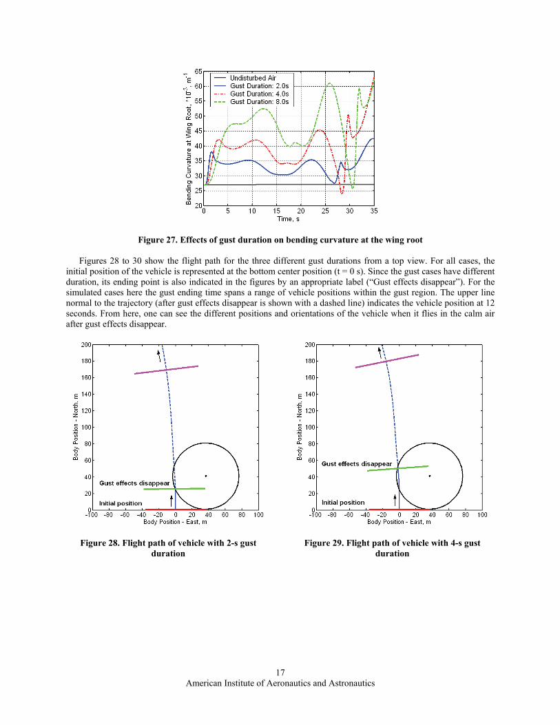
Figure 27. Effects of gust duration on bending curvature at the wing root Figures 28 to 30 show the flight path for the three different gust durations from a top view. For all cases, the

initial position of the vehicle is represented at the bottom center position (t = 0 s). Since the gust cases have different duration, its ending point is also indicated in the figures by an appropriate label (“Gust effects disappear”). For the simulated cases here the gust ending time spans a range of vehicle positions within the gust region. The upper line normal to the trajectory (after gust effects disappear is shown with a dashed line) indicates the vehicle position at 12 seconds. From here, one can see the different positions and orientations of the vehicle when it flies in the calm air after gust effects disappear.

Figure 28. Flight path of vehicle with 2-s gust duration



17


Another interesting observation can be made when one look at the above results for 25 seconds and beyond. The responses do not follow the same tendency as that before this time. This is because at approximately 25 seconds the different wing stations exceed the stall angle of attack, changing the vehicle response. The effects of stall on the vehicle can be assessed by turning off the stall module and comparing the results with and without stall effects. Keeping only the 10-m/s center amplitude and 4-s duration gust case, results are presented for vehicle responses considering stall on and off. With stall effects turned on, the aerodynamic loads on the airfoil are not continuous before and after the moment the stall. The discontinuity results in reductions in loads and the corresponding mid span bending curvature, as shown in Figs. 31 and 32, respectively. Although there is a sudden drop in lift around 27 s, the transient loads excite the vehicle to large deformations and eventually large root strains. The fact that the configuration has an unstable phugoid mode exacerbates the transient response and reaches higher bending curvatures levels. The impact of stall on vehicle response is illustrated in Figs. 33 to 38. The difference after 27 seconds can be clearly seen from those plots, where stall leads to increase in plunging motion (Fig. 35), as well as pitching angle (Fig. 37). Therefore, stall effects can have a significant impact on the trajectory and attitude predictions.

Figure 31. Lift distribution on the flying wing vehicle from 25 to 35 seconds (Left: Stall on, Right: Stall off)


18

Figure 32. Stall effects on bending curvature at the wing mid span location (root) when vehicle is subjected to

10-m/s center amplitude and 4-s duration gust

Figure 33. Stall effects on Westerly body position

when vehicle is subjected to 10-m/s center amplitude and 4-s duration gust

Figure 34. Stall effects on Northerly body position


Figure 35. Stall effects on body altitude when

vehicle is subjected to 10-m/s center amplitude and 4-s duration gust

Figure 36. Stall effects on Euler yaw angle when



19

Figure 37. Stall effects on Euler pitching angle when vehicle is subjected to 10-m/s center amplitude and

4-s duration gust

Figure 38. Stall effects on Euler roll angle when


It is expected that different gust amplitudes will have a different effect on the vehicle response. For the present

study, a similar gust perturbation but with maximum center amplitude of 5 m/s is applied and the results are compared with the 10 m/s as used before. Note that both gusts have the same duration of 2 seconds. Figure 39 presents the comparison of root bending curvature at the vehicle mid span station. It shows that the two cases have similar responses before 25 seconds, although with values directly proportional to the gust magnitude. However, the bending curvature of the 5-m/s gust response show more regular pattern up to 35 seconds, while the 10-m/s gust response show an increase of bending curvature after an initial sudden reduction right after 25 seconds. This variation in bending curvature is related with stall effects as discussed before. Notice, however, that the absence of this sudden reduction in the 5-m/s gust case does not mean there will not be any stall happening. Since the phugoid mode of the vehicle is unstable, fact reinforced by the responses shown in Figs. 42 and 44, the angle of attack will eventually grow to reach stall and a similar outcome to the 10-m/s gust response is anticipated.

Figure 39. Effects of gust amplitude on bending curvature at the wing mid span (root)


20

Figure 40. Effects of gust amplitude on body position - West

Figure 41. Effects of gust amplitude on body position - North

Figure 42. Effects of gust amplitude on body altitude

Figure 43. Effects of gust amplitude on Euler yaw angle

Figure 44. Effects of gust amplitude on Euler pitching angle

Figure 45. Effects of gust amplitude on Euler roll angle


21

E. Effects of Skin Wrinkling on Gust Response In this section, the effects of skin wrinkling on the gust response are investigated. From preliminary simulations,

the region most likely to reach higher curvature is located at the mid span (wing roots). Post-wrinkling torsional stiffness reductions are selected as 20% (TSR 1) and 40% (TSR 2) of the original one for this study. As discussed before, the threshold point between the two torsional stiffness states is determined by the corresponding flat bending curvature. The critical flat bending curvature is postulated to be 0.0298 m-1 (CFBC 1), which is 10% higher than the bending curvature of the vehicle at free level flight in calm air. Gust disturbance with 10-m/s center amplitude and 2-s duration is used.

Figures 46 to 48 show the vehicle positions, while Figs. 49 to 51 show the Euler body angles. It can be seen from the figures that the skin wrinkling mainly affects the lateral motion and the yaw angle of the body. If the torsional stiffness reduces to 60% of nominal value when skin wrinkles, the difference of lateral displacement at the end of 35 seconds is about 6.7 m, which is about 9.5% of the lateral displacement when skin wrinkling is not considered. The corresponding difference in yaw angle is about 1.5o, which is approximately 13.4% of the yaw angle when skin wrinkling is not considered. For the other responses, the effects of skin wrinkling are very small.

Figure 46. Effects of skin wrinkling on Westerly body position when vehicle is subjected to 10-m/s

center amplitude and 2-s duration gust

Figure 47. Effects of skin wrinkling on Northerly body position when vehicle is subjected to 10-m/s

center amplitude and 2-s duration gust

Figure 48. Effects of skin wrinkling on body altitude


Figure 49. Effects of skin wrinkling on Euler yaw angle when vehicle is subjected to 10-m/s center

amplitude and 2-s duration gust


22

Figure 50. Effects of skin wrinkling on Euler pitch

angle when vehicle is subjected to 10-m/s center amplitude and 2-s duration gust

Figure 51. Effects of skin wrinkling on Euler roll angle when vehicle is subjected to 10-m/s center

amplitude and 2-s duration gust

IV. Concluding Remarks A methodology to study the coupled nonlinear flight dynamics and nonlinear aeroelastic response of highly-

flexible flying wings to gust response was presented. The geometrically-nonlinear structural model is a strain-based formulation, which is able to capture the large deformations in slender structures. Incompressible unsteady aerodynamics with simplified stall models is coupled with the structural formulation, which completes the aeroelastic formulation. Nonlinear equations of motion for a frame associated to the vehicle (not necessarily at its c.g.) complete the coupled flight dynamics/aeroelastic formulation. The resulting differential equations are then integrated in time. The formulation includes models for non-symmetric, spatially-distributed gust and bi-linear wing torsional stiffness associated with skin wrinkling effects due to large wing bending.

A detailed study was conducted of the dynamic response of a highly-flexible flying wing previously presented in the literature. Responses under maneuver perturbation and gust disturbance were obtained using the proposed formulation. Effects of gust, stall, and wing skin wrinkling were evaluated for this particular numerical example.

The sample vehicle was trimmed at different payload conditions. Linear stability analysis was performed by solving the linearized system of equations at trimmed conditions. From it, the phugoid mode eventually became unstable with the increase on payload. The short period mode was purely real for the range of payloads considered. Fully nonlinear time-marching simulation was performed with an initial flap perturbation from trim condition. The unstable phugoid mode was clearly excited, which may compromise the performance and integrity of such vehicle.

Vehicle response to gust was analyzed for different gust amplitudes and duration. As expected, flight path, vehicle attitude and structural motion were impacted by the presence of gust. The disturbed flight path went away from the gust center. Furthermore, the plunging and pitching motions were both excited by the gust and, since they were unstable, resulted in increasing amplitude response with time. Large plunging and pitching motions of the vehicle with corresponding large elastic deformations also resulted in high instantaneous angles of attack on some stations along the wing. The effects of stall had a significant impact on the sample flying wing dynamic response and should be taken into account when analyzing this type of vehicles. Knowledge of the actual airfoil stall characteristics at different Reynolds number should take into account when analyzing for stall effects. Finally, the skin wrinkling connection with the wing torsional stiffness showed to mainly affect the motions of the vehicle in the lateral direction. For the other responses, the effects of skin wrinkling were small based on the parameters chosen for the numerical study.

V. Acknowledgements

The authors are grateful to Maj. Christopher Shearer, USAF (University of Michigan) for his help with the flight dynamics in NAST. This work was partially supported by NASA Dryden Flight Research Center under contract NND05AC19P. The technical monitor is Martin J. Brenner. The views expressed in this article are those of the


23

authors and do not reflect the official policy or position of the National Aeronautics and Space Administration or the U.S. Government.

References 1Wood, M. W. and Bauer, S. X. S., “Flying Wings / Flying Fuselages”, AIAA-2001-0311, 39th AIAA Aerospace Sciences

Meeting & Exhibition, Reno, Nevada, January 8-11, 2001. 2Begin, L., “The Northrop Flying Wing Prototypes”, AIAA-1983-1047, 1983. 3Weisshaar, T. A. and Ashley, H., “Static Aeroelasticity and the Flying Wing”, AIAA-1973-397, AIAA/ASME/SAE 14th

Structures, Structural Dynamics, and Materials Conference. Williamsburg, Virginia, March 20-22, 1973. 4Fremaux, C. M., Vairo, D. M. and Whipple, R. D., “Effect of Geometry, Static Stability, and Mass Distribution on the

Tumbling Characteristics of Generic Flying-Wing Models”, AIAA-1993-3615-CP, 1993. 5Esteban, S., “Static and Dynamic Analysis of an Unconventional Plane: Flying Wing”, AIAA Atmospheric Flight Mechanics

Conference and Exhibit, Montreal, Canada, August 6-9, 2001. 6Mialon, B., Fol, T. and Bonnaud, C., “Aerodynamic Optimization of Subsonic Flying Wing Configurations”, 20th AIAA

Applied Aerodynamics Conference, St. Louis, Missouri, June 24-26, 2002. 7Sevant, N. E., Bloor, M. I. G. and Wilson, M. J., “Aerodynamic Design of a Flying Wing Using Response Surface

Methodology”, Journal of Aircraft, Vol.37, No.4, July - August 2000, pp 562 - 569. 8Patil, M. J., Hodges, D. H., and Cesnik, C. E. S., “Nonlinear Aeroelasticity and Flight Dynamics of High-Altitude Long

Endurance Aircraft,” Journal of Aircraft. Vol. 38, No. 1 Jan. - Feb. 2001. 9van Shoor, M. C., Zerweckh, S. H. and von Flotow, A. H., “Aeroelastic Stability and Control of a Highly Flexible Aircraft”,

AIAA Paper, AIAA-89-1187-CP, 1989. 10Drela, M., “Integrated Simulation Model for Preliminary Aerodynamic, Structural, and Control-Law Design of Aircraft”,

AIAA Paper, AIAA-99-1394, 1999. 11Love, M. H., Zink, P. S., Wieselmann, P. A. and Youngren, H., “Body Freedom Flutter of High Aspect Ratio Flying

Wings”, AIAA Paper, AIAA-2005-1947, AIAA/ASME/ASCE/AHS 46th Structures, Structural Dynamics, and Materials Conference. Austin, Texas, April 18-21, 2005.

12Noll, T. E., Brown, J. M., Perez-Davis, M. E., Ishmael, S. D., Tiffany, G. C., and Gaier, M., “Investigation of the Helios Prototype Aircraft Mishap. Volume 1, Mishap Report”, NASA Report, Jan., 2004.

13Hoblit, F. M., “Gust Loads on Aircraft: Concepts and Applications”, AIAA Education Series, AIAA, Washington, DC, 1988, pp. 29-46.

14Chen, P. C., “Nonhomogeneous State-Space Approach for Discrete Gust Analysis of Open-Loop / Closed-Loop Aeroelastic Systems,” AIAA-2002-1715, AIAA/ASME/ASCE/AHS/ASC 43rd Structures, Structural Dynamics, and Materials Conference. Denver, Colorado, April 22-25, 2002.

15Lee, Y. -N. and Lan, C. E., “Analysis of Random Gust Responses with Nonlinear Unsteady Aerodynamics”, AIAA Journal, Vol. 38, No. 8, August, 2000, pp 1305 - 1312.

16Patil, M. J. and Hodges, D. H., “Flight Dynamics of Highly Flexible Flying Wings,” International Forum on Aeroelasticity and Structural Dynamics, 2005, Munich, Germany, June 28 – July 1, 2005.

17Radcliffe, T. O. and Cesnik, C. E. S, “Aeroelastic Response of Multi-Segmented Hinged Wings,” AIAA Paper, AIAA-2001-1371, AIAA/ASME/ASCE/AHS 42th Structures, Structural Dynamics, and Materials Conference. Seattle, Washington, April 16-19, 2001.

18Cesnik, C. E. S. and Brown, E. L., “Active Warping Control of a Joined Wing Airplane Configuration,” Proceedings of the 44th Structures, Structural Dynamics, and Material Conference, Hampton, Virginia, April 7 - 10, 2003.

19Cesnik, C. E. S. and Su, W., “Nonlinear Aeroelastic Modeling and Analysis of Fully Flexible Aircraft,” AIAA Paper, AIAA-2005-2169, AIAA/ASME/ASCE/AHS 46th Structures, Structural Dynamics, and Materials Conference. Austin, Texas, April 18-21, 2005.

20Peters, D. A. and Johnson, M. J., “Finite-State Airloads for Deformable Airfoils on Fixed and Rotating Wings”, Symposium on Aeroelasticity and Fluid/Structure Interaction/Proceedings of the Winter Annual Meeting, AD Vol. 44, American Society of Mechanical Engineers, Fairfield, NJ, 1994, pp.1-28.

21Shearer, C. M. and Cesnik, C. E. S., “Nonlinear Flight Dynamics of Very Flexible Aircraft”, AIAA 2005-5805, AIAA Atmospheric Flight Mechanics Conference and Exhibit, August 15 - 18, 2005, San Francisco, California, 2005.

22Hénon, M., “On the Numerical Computation of Poincaré Maps”, Physica D, Vol. 5, 1982, pp. 412-414.


24

dynamic response of highly flexible flying wings

Documents