flight evaluation of center-tracon automation system ... · flight evaluation of center-tracon...
TRANSCRIPT

NASA/TP-1998-208439
Flight Evaluation of Center-TRACON
Automation System Trajectory PredictionProcess
David H. Williams
Langley Research Center, Hampton, Virginia
Steven M. Green
Ames Research Center, Moffett Field, California
National Aeronautics and
Space Administration
Langley Research CenterHampton, Virginia 23681-2199
July 1998
https://ntrs.nasa.gov/search.jsp?R=19980210598 2018-07-13T04:50:22+00:00Z

Available from the following:
NASA Center for AeroSpace Information (CASI)7121 Standard Drive
Hanover, MD 21076-1320
(301) 621-0390
National Technical Information Service (NTIS)
5285 Port Royal Road
Springfield, VA 22161-2171
(703) 487-4650

Contents
Abbreviations and Symbols ........................................................... v
1. Summary ....................................................................... 1
2. Introduction ..................................................................... 1
3. Background ..................................................................... 2
3.1. Center-TRACON Automation System ............................................. 2
3.2. CTAS Trajectory Prediction Process .............................................. 3
3.3. Error Sources ................................................................. 3
4. Experiment Design ............................................................... 4
4.1. Objective .................................................................... 4
4.1.1. Phase I ................................................................... 4
4.1.2. Phase II .................................................................. 4
4.2. Approach .................................................................... 4
4.3. Flight Test Area ............................................................... 5
4.3.1. Phase I ................................................................... 5
4.3.2. Phase II .................................................................. 6
4.4. Research System .............................................................. 6
4.4.1. TSRV Airplane ............................................................ 6
4.4.2. CTAS System ............................................................. 7
4.5. Test Procedures ............................................................... 7
4.6. Data Recording ............................................................... 8
4.6.1. Measured Data ............................................................ 8
4.6.2. Predicted Data ............................................................. 8
5. Test Conditions .................................................................. 8
5.1. Phase I ...................................................................... 9
5.1.1. Idle Descent .............................................................. 9
5.1.2. Constrained Descent ........................................................ 9
5.1.3. Test Matrix .............................................................. l0
5.2. Phase II .................................................................... 10
5.2.1. Conventional non-FMS ..................................................... 11
5.2.2. Conventional FMS ........................................................ 11
5.2.3. FMS With CTAS TOD ..................................................... 12
5.2.4. Range-Altitude Arc ........................................................ 135.2.5. Test Matrix .............................................................. 13
6. Results and Discussion ........................................................... 13
6.1. Error Sources ................................................................ 14
6.1.1. Radar Tracking Errors ...................................................... 14
6.1.2. Airplane Performance Model Errors ........................................... 16
6.1.3. Atmospheric Modeling Errors ............................................... 176.1.4. Pilot Conformance ........................................................ 18
6.1.5. Experimental System Errors ................................................. 18
6.2. CTAS Trajectory Prediction Accuracy ............................................ 20
6.2.1. Cross-Track Profile ........................................................ 21
6.2.2. Along-Track Profile ....................................................... 21
too
Ill
6.2.3. Altitude Profile ........................................................... 21
6.2.4. Speed Profile ............................................................. 23
6.2.5. Time Profile ............................................................. 24
6.3. Sensitivity Analysis ............................................................ 26
6.4. Qualitative Impact of Error Sources ................................................ 27
6.4.1. Radar Track .............................................................. 27
6.4.1.1. Position .............................................................. 27
6.4.1.2. Speed ................................................................ 27
6.4.1.3. Track angle ........................................................... 28
6.4.2. Atmospheric Model ....................................................... 28
6.4.2.1. Wind component along path ............................................. 28
6.4.2.2. Wind gradient along path ................................................ 28
6.4.2.3. Temperature .......................................................... 29
6.4.3. Airplane Performance Modeling .............................................. 296.4.4. Pilot Conformance ........................................................ 29
6.4.4.1. Navigation ............................................................ 29
6.4.4.2. Speed ................................................................ 297. Recommendations ............................................................... 30
8. Concluding Remarks ............................................................. 31
Appendix--TSRV Performance Model Update .......................................... 33
References ....................................................................... 40
Tables .......................................................................... 42
Figures .......................................................................... 49
iv
Abbreviations and Symbols
ADS
ARTCC, Center
ATC
accel
BOD
BODG
CD
CD,m
CAS
CDI
CDU
CRT
CTAS
D
DA
DME
decel
EPR
FAA
FAST
FFD
FL
FMS
GPS
g
HA
h
hpIC
IP
J
KCAS
LA
LNAV
M
MAG
MAPS
MCP
automatic dependent surveillance
Air Route Traffic Control Center
Air Traffic Control
acceleration
bottom-of-descent
bottom-of-descent gate
drag coefficient, DragqSref
performance model drag coefficient
calibrated airspeed
course deviation indicator
control and display unit
cathode ray tube
Center-TRACON Automation System
airplane drag, lb
Descent Advisor
distance measuring equipment
deceleration
engine pressure ratio
Federal Aviation Administration
Final Approach Spacing Tool
forward flight deck
flight level
Flight Management System
Global Positioning System
acceleration of gravity, 32.17 ft/sec 2
high altitude
true altitude, ft
pressure altitude, ft
initial condition
initial position for a test run
jet route
knots calibrated airspeed
low altitude
lateral navigation
Mach number
magnetic
Mesoscale Analysis and Prediction System
mode control panel

MF
Nmag
NASA
ND
NOAA
PD
PFD
PGA4D
PGUI
q
RFD
RTA
Fills
Srefstd. dev.
T
ark
rk,sTAS
TMA
TMD
TMU
TOC
TOD
TODG
TRACON
TRK
TSRV
UTC
VaVwVCSS
VNAV
VOR
W
8am
Y
4D
metering fix
magnetic north
National Aeronautics and Space Administration
navigation display
National Oceanographic and Atmospheric Administration
pilot discretion
primary flight display
profile generation algorithm, 4D
planview graphical user interface
free-stream dynamic pressure, lb/ft 2
research flight deck
required time of arrival
root-mean-square
reference wing area, ft2
standard deviation
airplane net thrust, lb
atmospheric temperature, K
standard day atmospheric temperature, K
true airspeed
Traffic Management Advisor
airplane net thrust minus drag, T - D, lb
Traffic Management Unit
top of climb
top of descent
top-of-descent gate
Terminal Radar Approach Control
track
Transport Systems Research Vehicle
universal time coordinated
true airspeed, ft/sec
wind speed, ft/sec
velocity control stick steering
vertical navigation
very high frequency omnidirectional radio range
weight, lb
atmospheric ambient pressure ratio
air-mass flight path angle, rad
four dimensional, time being the fourth dimension
A dot over a symbol denotes derivative with respect to time.
vi

1. Summary
The Center-TRACON Automation System
(CTAS), under development at the Ames Research
Center, is designed to assist controllers with the
management and control of air traffic in the extendedterminal area. The Langley Research Center is partici-
pating in a joint program with Ames to investigate the
issues of and develop systems and procedures for the
integration of CTAS and airborne automation systems.A central issue in this research is the accuracy of the
CTAS trajectory prediction process and compatibility
with airborne Flight Management Systems for the
scheduling and control of arrival traffic.
Two flight experiments were conducted (Phase I
in October 1992 and Phase II in September 1994) at
Denver to evaluate the accuracy of the CTAS trajec-
tory prediction process during the en route arrival
phase of flight. The Transport Systems Research
Vehicle (TSRV) Boeing 737 airplane based at the
Langley Research Center flew a combined total of 57
arrival trajectories from cruise altitude to a terminal-
area metering fix while following CTAS descent
clearance advisories. Actual trajectories of the airplane
were compared with the trajectories predicted by the
CTAS trajectory synthesis algorithms and airplane
Flight Management System. Trajectory prediction
accuracy was evaluated over several levels of cockpit
automation, which ranged from a conventional cockpit
to a performance-based vertical navigation (VNAV)
Flight Management System. Error sources and theftmagnitudes were identified and measured from the
flight data.
The CTAS descent advisor was found to provide a
reasonable prediction of metering fix arrival time per-
formance during these tests. Overall arrival time errors(Mean + Standard deviation) were measured to be
approximately 24 sec during Phase I and 15 see duringPhase II. The major source of error during these tests
was found to be the predicted winds aloft used by
CTAS. Position and velocity estimates of the airplane
provided to CTAS by the Air Traffic Control (ATC)
Host radar tracker were found to be a relatively insig-
nificant error source. Airplane performance modeling
errors within CTAS were found to not significantlyaffect arrival time errors when the constrained descent
procedures were used. The most significant effect
related to the flight guidance was observed to be the
cross-track and turn-overshoot errors associated with
conventional VOR (very high frequency omnidirec-
tional radio range) guidance. Lateral navigation
(LNAV) guidance significantly reduced both thecross-track and turn-overshoot errors. Pilot procedures
and VNAV guidance were found to significantlyreduce the vertical profile errors associated with atmo-
spheric and airplane performance model errors.
2. Introduction
Since 1989, a joint program has been underway
between the Ames Research Center and the Langley
Research Center to investigate the issues of and
develop systems for the integration of Air Traffic
Control (ATC) and airborne automation systems.
Ames has developed the Center-TRACON Automa-
tion System (CTAS), a ground-based ATC automation
system designed to assist controllers in the efficient
handling of traffic of all types and capabilities (ref. 1).
This system has the ability to accurately predict air-
plane trajectories and determine effective advisories toassist the controller in managing traffic. Langley has
been conducting and sponsoring research on flight
operations and Flight Management Systems (FMSs) of
advanced transport airplanes for a number of years.
During the course of this joint research, opera-
tional issues have been a primary concern; these
include the practical integration of Flight Management
System concepts to permit fuel efficient operations ina time-based ATC environment. The primary focushas been on the transition from en route cruise to the
arrival phase of flight because of the significantimpact of terminal area constraints on the en route tra-
jectory. Concepts for airplane-ATC automation inte-
gration were evaluated in two real-time piloted-
cockpit ATC simulations described in references 2
through 5. Early studies focused on the developmentand evaluation of automation functions and proce-
dures for integrating CTAS, FMS, and data-link sys-
tems in the extended terminal area. The emphasis was
on time-based traffic management, long lead-time
(approximately 20 min) conflict prediction, and effi-cient conflict resolution in the en route and arrival
phases of flight.
A central issue to integration of FMS and ATC
automation is the accuracy of the trajectory prediction
process used by each system. CTAS uses trajectory

predictionsof each airplane to schedule arrivals,
ensure conflict-free trajectories, and provide suggested
speed, altitude, and routing clearances to maximize
throughput with minimum deviation from user prefer-
ences. Airborne FMS trajectory predictions axe used to
provide economical flight profiles which satisfy air-
plane performance restrictions while adhering to oper-ational constraints.
Early piloted-simulation testing of CTAS trajecto-
ries with airline flight crews demonstrated favorable
results in terms of arrival time accuracy at a terminal-
area metering fix (refs. 6 and 7). These tests, however,
evaluated CTAS trajectory predictions based on ideal
knowledge of airplane state, airplane performance,
and atmospheric characteristics (winds and tempera-
tures aloft). The next step was to evaluate CTAS tra-
jectory prediction accuracy under realistic field
conditions including the errors associated with radar
tracking, airplane performance modeling, and atmo-
spheric modeling.
The establishment of CTAS field sites at several
FAA ATC facilities provided an opportunity to exer-cise CTAS under actual traffic and weather condi-
tions. However, accurate airplane and atmospheric
state information was not available for trajectory pre-
diction validation. Following the initial fielding ofCTAS at the Denver Air Route Traffic Control Center
(ARTCC or Center), it was recognized that the Trans-
port Systems Research Vehicle (TSRV) Boeing 737
airplane based at Langley Research Center could beused for actual flight test verification of the CTAS tra-
jectory prediction process. Use of the TSRV airplane
provided several advantages including the opportunity
to exercise CTAS clearance advisories (with minimum
impact on the airspace users), a platform for the accu-
rate measurement of actual airplane and atmospheric
state, and the ability to evaluate new cockpit proce-
dures in a flight environment.
Ames began conducting field tests of the descent
advisor (DA) portion of CTAS in 1992. Designed for
Center airspace, DA provides clearance advisories for
traffic management restrictions (e.g., metering) while
assisting the controller with the detection and resolu-
tion of conflicts between airplanes in all phases of
flight (ascent, cruise, and descent). The primary goal
of these tests was to evaluate the accuracy of the
CTAS trajectory prediction process for the en route
arrival phase of flight. Two TSRV flight experiments
were conducted: Phase I in October 1992 and Phase II
in September 1994.
This report describes both phases and presents
results in terms of the trajectory prediction accuracy
and the sources and magnitudes of trajectory predic-tion errors. Although the combined flight test data set
is not large enough to be statistically significant, the
data do provide insight into the size and impact oferrors associated with trajectory prediction under real-
world operating conditions. These data can be used as
input and validation for trajectory sensitivity studies to
determine the statistical representation of errors
(refs. 8, 9, and 10). The results of such studies can be
used to guide improvements to prediction algorithms
and data sources (e.g., prediction of atmospheric char-
acteristics and airplane tracking), determine the appro-priate buffers for conflict prediction, and develop
trajectory prediction error models for real-time analy-
sis of conflict probability.
3. Background
Capacity and efficiency improvements in the
national airspace system are needed to cope withincreased traffic demand and ensure the economic via-
bility of the air transportation industry. Airborne flight
management systems have been developed to provide
cost-efficient flight guidance for individual airplane
operations. Air traffic control automation tools
(decision support tools) are currently being designed
to assist controllers in achieving greater efficiencywith current ATC procedures as well as enable the
introduction of new, more efficient procedures. Suchtools include conflict prediction and resolution tools,
for allowing more user-preferred flight paths, and
time-based traffic management tools for minimizing
delay. Both the FMS and ATC automation systems
share the common need for accurate prediction of air-
plane flight trajectories in order to achieve their
respective performance goals. The focus of this publi-
cation is on the CTAS trajectory prediction process,
with reference and comparison with airborne FMS asdeemed appropriate.
3.1. Center-TRACON Automation System
CTAS is an integrated system comprised of three
tools that provide computer-generated advisories for
both en route (Center) and terminal (TRACON) con-trollers (ref. 1). The three tools include the Traffic
Management Advisor (TMA), the Descent Advisor

(DA), andtheFinalApproachSpacingTool (FAST).
These tools are designed to assist controllers in
achieving greater efficiency in the management andcontrol of arrival traffic in the extended terminal area
as well as assist in the conflict prediction and resolu-
tion of traffic along airway and user-preferred trajecto-
ties. As flights approach their destination (e.g., within
200 n.mi.), DA predicts the trajectories of airplanes in
Center airspace. The TMA then generates sequences
and schedules for arriving flights including those that
originate from nearby feeder airports. DA iterates on
speed profile, in addition to path and altitude, to
provide the Center controller with clearance advisoriesthat meet the TMA schedule with fuel-efficient cruise
and descent profiles. DA conflict prediction and
resolution tools assist the controller in separating
traffic in all en route phases of flight (climb, cruise,
and descent) while minimizing clearance changes. As
airplanes enter the terminal area, FAST updates the
sequences and schedules and provides TRACON con-
trollers with advisories for runway assignment,
sequence, headings, and speeds to optimize the deliv-
ery of airplanes to the runways.
3.2. CTAS Trajectory Prediction Process
The trajectory prediction process is the foundation
of CTAS. Because it has been developed from an air-
borne FMS concept, the CTAS trajectory prediction
process is similar in many ways to that employed for
an FMS. Whereas an FMS application tends to focus
on trajectory optimization for a single airplane, the
ATC application must also consider the interrelation-
ships of trajectories of multiple flights. The ATCapplication goes beyond the single focus of required
time of arrival (RTA) for time-based traffic manage-
ment and must consider separation between neighbor-
ing flights along entire trajectories not just at
procedurally controlled focal points such as a metering
fix. The task of reliable conflict prediction along ran-
dom 4D trajectories is critical to achieving the benefits
associated with the "free-flight" concept (ref. 11). The
effectiveness and efficiency of conflict resolution
actions depend on the accuracy of the trajectory pre-dictions used for conflict detection.
CTAS trajectory synthesis begins with the trajec-
tory initial condition and a series of flight path con-
straints. The initial condition (position, altitude, and
velocity) is based on airplane track (radar or airplane
reported) or flight plan data. The set of flight path con-
straints is based on a series of waypoints and segments
which define the bounds of a horizontal path to the
runway or trajectory end-point. The horizontal pathprediction is based on the current state of the airplane,
flight plan, airspace procedures, and heuristics which
relate the current state of the airplane to the flight plan
and local ATC procedures. For exceptional caseswhere the CTAS heuristics do not match controller
intent, the controller may update the CTAS path pre-
diction with quick keyboard and graphical inputs that
are separate from the formal Host flight plan amend-
ments. The waypoint constraints, generated to comply
with ATC procedures as defined in a CTAS navigation
database, may include altitude, airspeed, course, and/or time.
CTAS trajectories are synthesized in two steps.First, a horizontal ground track is generated by curve
fitting the waypoints with a series of straight-line andcircular-turn segments. The waypoints are designated
as either "fly-by," or "fly-over" based on the CTAS
navigational database adapted for a particular airspace.
The turn segments are based on a parameterized bank
angle and an estimated ground speed. This ground
speed is computed from an airspeed profile and a wind
estimate along a simple kinematic altitude profile. The
airspeed profile is either inferred from a combination
of flight plan, controller input, and the CTAS databaseor selected for time-control iteration. Second, the alti-
tude and time profiles are computed by integrating a
set of simplified point-mass equations of motion along
the established ground track. Within Center airspace, a
detailed set of airplane performance models is used to
determine thrust, drag, and speed envelope as a func-tion of airplane type. The atmosphere is modeled with
a three-dimensional grid of wind, temperature, and
pressure (ref. 12). A detailed description of the CTAS
trajectory synthesis process is presented in ref-erences 13 and 14.
3.3. Error Sources
Trajectory prediction accuracy is the key for creat-
ing effective and efficient ATC advisories. Errors refer
to the difference between the predicted and actual air-
plane state along a flight path. Error sources include
the estimation of an airplane state (position and veloc-
ity) for initializing a trajectory prediction, trajectory
modeling, and clearance conformance. Trajectory

modelingincludesairplaneperformance(e.g.,thrust,drag,weight),flight procedures,atmospheric charac-
teristics (e.g., wind and temperature aloft), and trajec-tory generation algorithms.
Although both CTAS and FMS are subject to
errors, differences between the two systems depend onthe environment and application. If the basic trajectory
generation algorithms are assumed similar, the differ-
ences between FMS and CTAS predictions are prima-
rily due to differences in the sensors and modeling
databases used by either system. Whereas the most
accurate sensors for determining airplane position and
velocity are available to the FMS, ATC systems are
currently dependent on less-accurate radar tracking.
As for winds and temperature, FMS-equipped air-
planes typically have the most accurate data at the cur-
rent position of the airplane whereas ATC systems
have access to the latest prediction over the future
flight path, particularly the descent profile. Most FMS
systems allow the flight crew to enter forecast winds
and temperatures at each waypoint along a flight plan,
as well as at several altitudes spanning the descent
profile. A few newer airplanes support automatic
uplink of these winds and temperatures; however,
such data are rarely updated in flight and may be 3to 6 hr old upon entry. Regarding airplane perfor-
mance modeling, most FMS systems have extensive
performance data which may be "tuned" to the air-
frame and engine. In comparison, ATC systems must
rely on engineering data when available or synthesized
data when they are not. Given the current FAA flight
plan procedures, ATC systems must estimate weight
(usually known to the FMS) and must categorize air-
planes within FAA designated types. Many of the dif-
ferences between CTAS and a particular FMS may be
mitigated through the use of data exchange to provide
increased precision between the air and ground com-
putations as well as an overall increase in trajectoryprediction accuracy (ref. 15).
4. Experiment Design
4.1. Objective
The primary objective of the flight tests was the
evaluation of CTAS trajectory prediction accuracy for
the en route arrival phase of flight, including identifi-
cation and measurement of significant potential error
sources. Secondary objectives included investigationof flight procedures as well as the application of cock-
pit automation tools for improving flight precision indescent.
4.1.1. Phase I
Phase I, October 1992, focused on straight-path
descents with an emphasis on the analysis of modeling
errors. In addition, the basic descent procedures testedin simulation would be used for the first time in a
flight environment. Flight-idle descent procedureswere used to isolate modeling errors, and "con-
strained" descents were flown to investigate flight pro-cedures for efficient vertical profile control to a
required altitude and speed at a fix. Constrained-
descent procedures were evaluated with and without
cockpit automation for visualizing the bottom-of-
descent crossing restriction. A limited FMS capability,consisting of lateral navigation (LNAV) and guidance
along the straight path and navigation map display of
range to intercept of a selected altitude, was used for
the cockpit automation in Phase I.
4.1.2. Phase H
The primary objective of Phase II, September
1994, was to evaluate CTAS trajectory prediction
accuracy along a more complex arrival route with
expanded flight procedures and a wider range of FMS
capability for LNAV and performance-based vertical
navigation (VNAV). The arrival route was chosen to
provide a large turn during the middle of the descent.
Previous simulation testing at Ames (ref. 6) had
shown that pilots without LNAV exhibit a tendency to
overshoot the turn and subsequently fly a longer than
predicted path. Imprecision in the pilot overshoot pre-
sents an additional challenge in accurately predicting
the lateral path of a conventionally equipped airplane.The intent was to determine whether the lateral errors
observed in the earlier simulation tests and the vertical
errors observed in Phase I could be reduced by
improved piloting procedures and what additional
improvement could be gained by utilizing FMS
LNAV and VNAV capability. A secondary objective
of Phase II was to sample actual atmospheric condi-
tions for comparison with the CTAS model along thearrival test route as well as at additional locations in
the test airport vicinity.
4.2. Approach
The test was designed to expose DA to realisticmodeling errors under field conditions with minimum
4

impacton the ATC facility andcommercialflightoperations.Duringboth testphases,theTSRVwas
operated on an arrival flight plan tailored to replicate a
typical commercial airline arrival at Denver. Each test
flight consisted of several test runs conducted by using
a closed-circuit routing designed to maximize theamount of data collected on a given flight. The TSRV
was flown from both the forward flight deck, repre-
senting a conventionally equipped airplane (e.g.,
Boeing 737-200, Boeing 727-200, McDonnellDouglas DC-9/MD-80), and the research flight deck,
representing an FMS-equipped airplane (e.g., Boeing
737-400, Boeing 757/767).
Test runs were conducted during low traffic peri-
ods to minimize the impact on commercial flight oper-
ations and to allow the TSRV to conduct uninterrupted
descents. Although interruptions commonly occur as apart of normal ATC operations, isolating the TSRVwas desirable to enable identification and measure-
ment of trajectory prediction error sources. CTAS was
operated by a test engineer due to the absence, at thattime, of an FAA-approved CTAS interface for the
radar controllers. The approach was for the TSRV
pilot and controller to coordinate pilot discretion (PD)
descents while the CTAS operator relayed the DAadvisories to the TSRV over a dedicated (non-ATC)
frequency.
CTAS was operated with data sources that repre-
sent the quality of data available to a current opera-
tional system. Airplane track and flight plan data were
obtained by CTAS through established operationalinterfaces to the ATC Host computer. For the TSRV
airplane, CTAS used manufacturer's performancedata. The performance data included drag, thrust, and
fuel consumption as a function of airplane and atmo-
spheric state. Atmospheric data (winds and tempera-
ture aloft) were obtained from the National
Oceanographic and Atmospheric Administration
(NOAA) Mesoscale Analysis and Prediction System
(MAPS) (ref. 16). MAPS is the research prototype
version of the Rapid Update Cycle (ref. 17) operated
by the National Center for Environmental Prediction
(NCEP), formerly the National Meteorological Center
(NMC).
For Phase II, the TSRV FMS used data from dif-
ferent sources than CTAS, which were also the most
accurate sources of data available. Airplane state data
were taken directly from airplane measurements,
atmospheric data were entered into the FMS by handbased on the measurements of previous runs, and the
performance data were based on data from earlier
flight tests. These differences in input data betweenCTAS and the TSRV FMS were used to ensure differ-
ences in the respective trajectory predictions. This
approach provided two advantages:
1. It would highlight the potential differences
between CTAS and FMS trajectories under
operational conditions
2. It would provide insight into the sensitivity of
trajectory prediction accuracy to the accuracy ofthese data sources
Airplane state and observed atmospheric data
were recorded onboard the TSRV airplane for post-
flight comparison with the real-time CTAS trajectory
predictions, airplane track, and MAPS data. Through-out this report, the term "actual" refers to the measure-
ments made onboard the TSRV airplane with the
Global Positioning System (GPS) navigation system.
4.3. Flight Test Area
4.3.1. Phase I
The area of test operations for Phase I, including
the nominal flight path of the airplane, is shown in fig-ure 1. The test was confined to one area (group of sec-
tors) within Denver Center and primarily involved tworadar sectors. The high altitude sector 9 (HA9) sets the
sequence of arrivals from the northeast and controls
the airspace including flight level (FL) 240 and above.
Arriving flights are typically handed off to the lowaltitude sector 15 (LA15) for metering into the Denver
TRACON via the KEANN metering fix.
A flight plan was developed, with the assistance ofthe Denver Center and TRACON controllers, to allow
for a closed-circuit routing using jet route 10 (J10) for
the test runs and the airspace southeast of J10 for
climb out and prerun maneuvering. The nominal plan
was to depart from Denver Stapleton International
Airport, proceed direct to AKO (Akron VOR station),direct to LEWEL, direct to PONNY, direct to Denver
Airport. The test run was conducted between the ini-
tial point (IP) at PONNY and the TRACON boundary
5

at KEANN. The actual flight path between AKO and
PONNY varied from run to run, depending on the
climb performance of the TSRV and traffic condi-tions, to enable the TSRV to be stabilized in cruise atthe IP. Descents were initiated from FL350 with a
metering fix crossing condition at KEANN of FL170at or below 250 KCAS. Pressure altitude was used
throughout the descent to remove the step change in
altitude effect from the data analysis for this test
phase. After crossing KEANN, the airplane wouldeither climb eastbound for another run or return to
Denver for landing.
4.3.2. Phase H
Figure 2 illustrates the Phase II area of test opera-tions along with the nominal flight path. This test was
conducted primarily in the northwest area. The high
altitude sector HA14 sets the sequence of arrivals from
the northwest and controls the airspace including
FL240 and above. Arriving flights are typicallyhanded off to the low altitude sector LA13 for meter-
ing into the Denver TRACON via the DRAKO meter-
ing fix.
In Phase II, the primary test runs were flown along
J56 with the airspace to the south used for climb out
and prerun maneuvering. The descents were initiated
from FL330 with a metering fix crossing condition at
DRAKO of 17000 feet at or below 250 KCAS. During
Phase II, the proper altimeter setting was used to
determine metering fix crossing altitude. The initial
point for the primary test runs was at CHE (Hayden)VOR. A second route, beginning at IP2, joined the
arrival traffic inbound to the KEANN metering fix.This second route was used to obtain additional atmo-
spheric data with the TSRV from a different quadrant.Runs conducted along this secondary route were not
used to complete the primary test matrix of descent
trajectory cases.
4.4. Research System
way voice communication between the TSRV airplaneand the CTAS ground station.
4.4.1. TSRV Airplane
The airplane used in these tests was the TSRV air-
plane, a modified Boeing 737-100 (fig. 3). The TSRV
is a flying laboratory equipped with a research flight
deck (RFD) located in the cabin behind the conven-
tional forward flight deck (FFD), as shown in the cut-
away model of the airplane in figure 4. The interior of
the RFD is a full-size flight deck that features eight 8-
by 8-in. flight-quality, color CRT displays and side-
stick flight controllers (fig. 5). Experimental systems
used in the RFD consist of an electronic flight display
system, a digital fly-by-wire flight control and flight
guidance system, and an advanced area navigation
system with GPS sensor inputs. The airplane may beflown from either the RFD or FFD.
The TSRV airplane was equipped with a fully
capable four-dimensional (4D) navigation and guid-
mace system developed during the mid 1970's in sup-
port of the Terminal Configured Vehicle Program(ref. 18). This baseline system, however, did not
incorporate performance management features neces-
sary for computation of vertical trajectories. Ground
speeds and altitudes were required inputs to each way-
point in the guidance buffer of the flight management
computer. The system also lacked the flexibility of
flight plan generation and modification found in cur-
rent commercial flight management systems.
The system was upgraded in the late 1980's to
incorporate modern control display units, as illustrated
in figure 6. At the same time, expanded lateral flightplan generation capability was added which closely
approximated the functionality of commercial flight
management systems. In addition to the lateral naviga-
tion features, the navigation display included a range-
altitude arc for displaying the predicted intercept of a
desired altitude. This capability was used duringPhase I.
The primary equipment used for these tests con-
sisted of the TSRV airplane operating in the Denver
terminal area and the CTAS field system on the
ground at Denver Center. In addition to standard two-
way voice communication between the pilots andATC, a dedicated frequency was used to support two-
For Phase II, the capability was added to compute
vertical trajectories and provide vertical guidance sim-
ilar to the commercial Boeing 737-300 commercialsystems. This was accomplished with the NASA-
developed profile generation algorithm (PGA4D)
described in references 2 and 4. The time-control (4D)

modewas not implemented for this test. In addition,the range-altitude arc was augmented with the capabil-
ity to display the projected altitude intercept along a
curved path, as shown in figure 7.
Selection of flight guidance and control modes in
the RFD are made through the mode control panel
(MCP) located in the center of the glare shield (fig. 8).
A description of the MCP and baseline guidancemodes available in the RFD may be found inreference 19.
4.4.2. CTAS System
Figure 9 illustrates the test setup within the
Denver Center. The CTAS station, located adjacent to
the Traffic Management Unit (TMU) on the control
room floor, was comprised of a distributed network of
Sun Microsystems Sparc-10 workstations. Real-time
updates of radar track and flight plan data for arrivals
were received from the FAA Host computer via a one-
way (Host-to-CTAS) interface. Radar track data (posi-
tion, mode-C altitude, and velocity) were nominally
updated by the Host computer on a 12-sec cycle.
MAPS forecasts of winds and temperatures aloft were
received from NOAA on a 3-hr update cycle. These
forecast updates were received (and used) by CTAS
approximately 30 min prior to the forecast period.
Host track data were displayed on a CTAS plan view
graphical user interface (PGUI) with DA advisory data
superimposed on the display in both tabular and color
graphical form (ref. 20).
For the purposes of these flight tests, the descent
speed profiles for the TSRV airplane were selectedfrom a test matrix to provide a controlled set of speed
profile conditions to support the analysis of trajectoryprediction accuracy. The test matrix speed profiles
were input to DA for each run and used to compute a
top-of-descent (TOD) clearance advisory. Additional
DA functionality, including advisories for cruise
speed, cruise altitude, direct headings, delay vectors,and conflict detection and resolution, was not evalu-ated in these tests.
Prior to both Phases, the CTAS/DA trajectory cal-
culations were validated against the FMS/PGA4D cal-
culations. The validation was based on running a
series of trajectory predictions, over a range of speed
profiles, for a common set of input data (atmosphericconditions and performance data). The comparison
trajectories were based on a nominal flight distance of
100 n.mi. with descents that were on par with those to
be explored in the flight tests. Results indicated that
the two systems produced comparable trajectories
with no more difference than 1 n.mi. in top of descentand 2 sec in arrival time.
4.5. Test Procedures
The test procedures used during both Phases were
essentially the same. TSRV flights were coordinated
with Denver traffic management to allow multiple
descent runs during low traffic periods. A list of
desired test conditions (including speed profile and
cockpit procedure) was prepared prior to each flight.The desired test condition for each run was chosen
during the climb phase of the run. Selection of this test
condition was a function of the traffic situation, per-
formance capability of the airplane, fuel status, and
test matrix completion. During Phase I, the DA con-
flict probe was used by the test engineer to shadow thearrival traffic and determine which test conditions
would allow for an uninterrupted descent. The highaltitude controller would then issue radar vectors to
the TSRV, prior to the IP, to allow a pilot discretiondescent without traffic conflicts. A traffic managementcontroller coordinated test activities between the
CTAS station and each participating radar sector.
The CTAS test engineer monitored the progress of
the TSRV airplane on the DA PGUI. After the air-
plane crossed the IP, the TSRV test engineer would
report the CAS, ground speed, and measured wind for
comparison with the test condition and CTAS esti-mates of the same variables. When the airplane was
stable at the desired cruise speed, the CTAS engineer
would relay the approximate TOD to the TSRV engi-
neer and high altitude controller. When the airplanewas nominally within 20 to 50 n.mi. of the TOD, the
CTAS trajectory was recorded and final TOD location
transmitted to the TSRV engineer. With the PD
descent clearance issued, the TSRV engineer would
relay the TOD to the flight crew to simulate the con-troller's issuance of a DA-based descent clearance.
Airborne measurements of actual airplane and atmo-
spheric state were recorded automatically on theTSRV.
The flight crew onboard the TSRV airplane con-sisted of two pilots in the FFD and a single pilot in the
7

left seatof the RFD. The right seat of the RFD was
occupied by the TSRV test engineer. All normal ATC
communications were handled by the FFD pilots.Communication with the CTAS workstation was han-
dled by the TSRV test engineer. Voice communica-
tions to both ATC and CTAS could be monitored by
all pilots.
Each test condition specified whether the runwould be flown from the FFD or the RFD. Prior to
reaching the IP waypoint, the flight crew in the appro-
priate cockpit would assume control of the airplane.
All FFD test runs were flown manually by the pilotswithout the use of autopilot or autothrottle. The RFD
pilot used manual control during Phase I and autopilotduring Phase 1I.
The pilot began each run by establishing the air-
plane in level cruise at the appropriate altitude and
speed for the test condition. Prior to top of descent, the
pilot was advised by the TSRV engineer of the desiredTOD in terms of DME distance from the Denver
VOR. The pilot would monitor DME distance and ini-
tiate descent upon reaching the specified range to Den-ver. The pilot conducted the descent by using the
profile descent tracking procedures specified by the
test condition (defined later). The test run ended when
the airplane reached the final altitude and speed and
crossed the MF waypoint (KEANN or DRAKO).
4.6. Data Recording
Two primary sets of data parameters were col-lected during these tests:
1. Measured conditions, such as airplane state and
atmospheric data
2. Predicted conditions, such as trajectory predic-
tions from CTAS DA and the airplane FMS aswell as predicted atmospheric conditions
Data recording onboard the airplane and at the CTAS
workstations was tagged to Universal Time (UTC) forpostflight correlation.
4. 6.1. Measured Data
The TSRV sensors provided airplane state data,
such as position (latitude and longitude), airspeed,
ground speed, altitude, body angles, and accelerations.
Wind speed and wind direction were computed in real
time based on airspeed, ground speed, and body
angles. Atmospheric temperature measurement was
also provided by the TSRV air data system. Most
parameters were updated and recorded at a rate of
20 Hz but were averaged over 1 see in postprocessing.
Airplane tracking data, including position (x,y coordi-
nates in the Denver Center reference frame), mode-C
altitude, track angle, and ground speed, were obtained
from the Denver Center Host computer with an
approximate update rate of one track report every
12 sec (ref. 21). Radar track position data were pro-
vided to CTAS in the Denver Center reference frame,
a stereographic coordinate system with the origin
approximately 700 n.mi. southwest of the Denver air-
port. For the purposes of comparison, TSRV positiondata were converted to the Denver Center reference
frame.
4.6.2. Predicted Data
Trajectory predictions were computed and
recorded by the CTAS DA for all test runs during both
Phases. In addition, the TSRV FMS computed and
recorded predicted trajectories for Phase II (FMS pre-dictions were not available in Phase I). Both sources
of trajectory predictions provided point-to-point four-dimensional trajectories for each descent from the ini-
tial position of the airplane up to and including themetering fix location. CTAS received and recorded
the 3-hr MAPS forecast on a 3-hr update cycle. This
forecast was received approximately 30 min prior to
the forecast period and was based on an analysis of the
atmosphere during the preceding period. CTAS
obtained the predicted winds and temperature along a
flight path by interpolating within the MAPS datagrid.
5. Test Conditions
The test conditions employed in both tests were
designed to provide a reasonable representation of
commercial airline jet transport descents as anticipated
in a CTAS Descent Advisor operational environment.
Cockpit automation and the corresponding pilot proce-
dures were studied to investigate their impact on the
descent trajectory. The NASA test pilots were
instructed to fly the descents as precisely as possible inorder to minimize pilot-induced variations in the

descent profiles. The goal was to emphasize the
differences between the systems (and associated
procedures).
5.1. Phase I
Two specific types of descent procedures wereused in Phase I: (1) idle descents, in which idle thrust
was used from TOD to BOD altitude and metering fix
crossing speed and (2) constrained descents in which
the pilot employed thrust and/or speed brake duringthe descent in order to achieve BOD altitude and air-
speed as closely as possible to the metering fix loca-
tion. The purpose of the idle descent procedure was to
provide a direct measurement of the trajectory predic-
tion accuracy of CTAS, which utilized an idle descent
model in the trajectory predictions for this test. Opera-tional versions of CTAS are anticipated to use a near-
idle thrust model for descent trajectory predictions to
match the procedures related to individual airplane
performance types and operating conditions. The con-
strained descent procedure represented a more realistic
procedure in which the pilot adjusts the altitude profilein descent to achieve the desired crossing conditions
(speed and altitude) at a waypoint assigned by ATC.
This procedure has the added benefit of mitigating the
impact of trajectory prediction errors by closing the
loop on the vertical profile. The idle and constraineddescents were flown from both the FFD and RFD. All
descents were flown manually since the TSRV was
not equipped with autopilot functions which held air-
speed by using pitch control. The specific procedures
used are detailed in the following paragraphs.
5.1.1. Idle Descent
The pilot procedures for idle descents were essen-tially the same for both the FFD and RFD. The pilot
would begin the idle descent procedure when the air-
plane reached the CTAS-specified TOD point. This
point was identified as a DME distance from the Den-
ver VOR. Following TOD, the pilot flew one of three
vertical profile types, depending on speed (fig. 10). If
the descent CAS was less than or equal to the cruise
CAS, the pilot flew a slow descent profile (fig. 10(a)).
At TOD, the pilot would immediately retard the throt-tle to idle and decelerate in level flight. Once the
descent speed was achieved, the pilot initiated a
descent while using pitch control to maintain airspeed.If the descent Mach was equal to the cruise Mach, the
pilot flew a nominal descent profile (fig. 10(b)). At
TOD, the pilot would immediately retard the throttle
to idle and initiate a descent while using pitch control
to maintain the Mach/CAS speed schedule. If the
descent Mach was greater than the cruise Mach, the
pilot flew a fast descent profile (fig. 10(c)). At TOD,
the pilot would immediately initiate a descent (nomi-
nally 3000 ft/min) while maintaining cruise thrust toaccelerate to the descent Mach. Once the descent
Mach was achieved, the pilot would retard the throttle
to idle while using pitch control to maintain the Mach/
CAS speed schedule.
As the airplane approached the metering fix cross-
ing altitude, the pilot would initiate a level-off deceler-
ation segment, depending on the descent speed and
metering fix crossing speed. If the speeds required a
deceleration, the pilot maintained idle throttle until the
airplane approached the metering fix speed and then
increased throttle as necessary to maintain speed until
crossing the metering fix. If no deceleration was nec-
essary, the pilot increased throttle as necessary to level
off and maintain the descent speed until crossing the
metering fix.
5.1.2. Constrained Descent
The pilot procedures for the constrained descents
were the same as for the idle descents up to the con-
stant CAS segment of the descent. Once the constant
CAS segment was established, the pilot would adjust
the descent angle to achieve a BOD point which was
just prior to the metering fix. The BOD location was
chosen by a rule of thumb, to allow 1 n.mi. of deceler-ation distance for each 10 knots of speed reduction
required to achieve the assigned crossing speed at the
metering fix.
The RFD pilot used the range-altitude arc on the
navigation display to target the desired BOD point
(fig. 7). This arc showed the range at which the air-
plane would reach the altitude selected on the mode
control panel at the current inertial flight path angle of
the airplane. The pilot would then adjust throttle and/
or speed brake to hold the descent CAS while target-
ing the desired BOD location.
The FFD pilot procedures for constrained descentswere somewhat more complex than the RFD proce-
dures since the FFD pilots had no direct indication of
the range at which they would reach the BOD altitude.Commercial crews typically use the 3:1 rule of thumb

to plan 3 n.mi.of descent path for every 1000 ft ofdescent. This rule works well in terms of workload
and fuel efficiency for a small range of descent speedswhich vary as a function of airplane type, weight, and
atmosphere. However, for the CTAS application, it is
desirable for ATC to specify descent speed to allow
for safe and efficient merging of arrivals. Under these
conditions, it is desirable to allow the flight path (e.g.,
TOD) to vary as a function of descent speed, type, and
atmosphere, much like an FMS would. For fuel-
efficient descents, the TOD and flight path angle may
vary as much as 30 to 40 percent over the speed enve-
lope of typical jet transport types. The challenge is for
the pilot to maintain a situational awareness of vertical
profile progress.
Paper charts and a custom-programmed hand cal-
culator were provided to the FFD pilots to assist in the
constrained descents. The charts provided tables of
DME distance, altitude, and corresponding flight path
angles for each of the descent speed conditions in the
test. The pilots would determine the required flightpath angle to achieve BOD altitude by noting their
altitude and DME distance when the airplane reached
the target descent CAS. With this flight path angle as a
reference, the pilots could then determine the proper
altitude at a given DME distance or conversely the
proper DME distance at a given altitude needed to
maintain the correct decent angle. The descent rate
could then be adjusted with throttle or speed brake,
depending on whether the airplane was below or
above the desired altitude. The programmed hand cal-culator provided the same information. Both the charts
and calculator were developed during local flight test-ing of the descent procedures as aids for the NASA
test pilots. They were not intended to represent opera-tional techniques for airline pilots to use for CTAS
descent advisories. Such operational procedures would
require careful development and testing with actualairline crews.
5.1.3. TestMatrix
The test matrix for Phase I, given in table 1, was
defined to evaluate CTAS trajectory prediction accu-
racy over two primary test variables: speed profile and
pilot procedure. Seven speed profiles were selected to
exercise the nominal speed envelope of the TSRV
while generating a representative set of constant-speedand variable-speed trajectory segments. This approach
was used to generate a balanced set of trajectory cases
for analysis of prediction accuracy as well as a broad
data set for evaluating the TSRV performance charac-
teristics. Each of the seven speed profiles was flown
by using the idle-thrust descent procedure. The first
three speed profile cases were repeated with the con-
strained descent procedures from both the FFD and
RFD. The goal was to complete two runs for each of
the 13 conditions combining speed profile and pilotprocedures.
5.2. Phase II
Test conditions for Phase II were designed to
expand on Phase I with an emphasis on evaluating
how to best utilize current FMS capabilities for con-strained descents within a CTAS environment.
Descents with tunas were of particular interest due to
the increased complexity of lateral and vertical profiletracking. Three different levels of FMS automation
were chosen to represent a cross section of FMS auto-marion capabilities available within the current com-
mercial fleet. These levels represent
1. Conventional airplanes (without FMS)
2. FMS-equipped airplanes with VNAV capability
3. FMS-equipped airplanes with range-altitude arc
capability
These levels of FMS automation were simulated byrestricting the usage of the FMS on the TSRV at thedefined levels.
Four sets of pilot procedures were developed forthe TSRV to take advantage of these levels of FMS
automation. These procedures included
1. Conventional non-FMS
2. Conventional FMS (using FMS TOD)
3. FMS with CTAS TOD
4. Range-altitude arc
The TSRV pilot procedures were not intended asexact prototypes for operational use because of the
10

significantdifferences in the TSRV FMS, pilot
interface devices (mode control panel, CDUs, and
side-stick flight controllers), and flight control mode
(velocity control stick steering) compared with typical
commercial equipment. Instead, the procedures were
designed to mimic as closely as possible the tech-
niques proposed for use by airline flight crews follow-
ing CTAS descent advisories. A focused investigation
of operational procedures and flight crew human fac-tors was beyond the scope of this test. However, an
evaluation of pilot procedures involving commercial
airline flights was conducted in parallel with this test
phase (ref. 22).
The test conditions flown in the RFD required sig-
nificant preparation and pilot training. The RFD mode
control panel was designed many years before the
development of the performance-based VNAV sys-
tems which are common on modem commercial flight
decks. The TSRV system is highly flexible, however,
and techniques were devised to closely approximate
the commercial FMS modes. Flight cards were devel-
oped for each test condition with an event sequence of
TSRV-specific procedures to be followed in order to
mimic the desired commercial FMS functionality. The
exact procedures and flight cards used in the test are
described in the following sections.
5.2.1. Conventional non-FMS
These conventional non-FMS procedures were
designed to represent airplanes which are not equipped
with flight management systems. They were flown by
the pilots in the FFD. One pilot was designated as theflying pilot and manually flew the airplane from the IP
to the metering fix. The other pilot in the FFD handled
the nonflying duties, including communication with
ATC and the TSRV and CTAS test engineers. A
TSRV test engineer (or observer) was located in the
jump seat behind the FFD to observe and assist incommunication.
The flying pilot established the airplane on theinbound leg of the flight plan at the desired cruise alti-
tude and speed prior to crossing the IP. Conventional
VOR guidance was used for lateral tracking of the
flight plan route. The pilot maintained altitude and
speed up to the CTAS TOD.
The CTAS TOD was identified as a DME distance
to a reference VOR station (DEN). The nonflying pilot
tuned a navigation radio to the appropriate station and
monitored the DME distance. The flying pilot was
instructed to begin the descent procedure within
0.1 n.mi. of the CTAS-specified DME range.
At the top of descent, the flying pilot would ini-
tiate the descent by retarding the throttle smoothly to
idle. If the descent speed was less than cruise speed,
the pilot would decelerate in level flight to achieve the
desired descent speed. The flying pilot flew the
remainder of the descent by using pitch to hold the
MactVCAS speed schedule. Prior to crossing 18000 ft,
the altimeter setting was changed to the local altimeter
setting. The pilots were instructed to target their BOD
to be just prior to crossing the metering fix. Throttle
and/or speed brake were used to adjust the descent rate
in order to reach BOD with just enough distance todecelerate from the descent CAS to the crossing speed
of 250 knots at the metering fix.
5.2.2. Conventional FMS
These conventional FMS descent procedures were
designed to utilize the VNAV capability of FMS-
equipped airplanes to generate and fly a VNAV pro-
file, including TOD, based on the CTAS-assigned
descent speed profile. They were flown from the RFD
by a NASA test pilot with the assistance of the TSRV
test engineer acting as the nonflying pilot. All RFD
test runs were flown by using autopilot for lateral
tracking of the FMS flight plan in order to provide
consistent performance for comparison with CTAS
horizontal path predictions.
The appropriate flight plan (company route) and
prestored approach were entered into the CDU prior to
reaching the IP for the test scenario. Measured wind
speed, wind direction, and static air temperature werehand recorded at intervals of 4000-ft altitude from
17000 to 33000 ft during the initial climb and on each
subsequent descent. The latest data were manually
entered into the descent wind page of the CDU for use
in the FMS trajectory prediction. (This approach
enabled using the FMS prediction to represent the
ideal case of minimum modeling error for trajectory
prediction, airborne or ground based.) Cruise speed
(Mach= 0.72 or 0.76, depending on test condition)
was entered as the selected speed on the CRUISE
CDU page, and the EXECUTE button pressed to
11

activatetheflight plan. The airplane was stabilized at
cruise altitude and speed prior to crossing the IP.
After crossing the IP, the appropriate test cardshown in figure 11 was used to specify the sequence of
activities in the RFD. As shown on the card, there
were six key events which required specific actions by
the pilot and test engineer. The test engineer would
monitor the events and call out the activities. The pilot
would cross-check and confirm the activities. Typi-
cally the test engineer would perform the activities
which required CDU entries and the pilot would han-dle mode control panel, throttle, and flight controller
inputs. The test engineer would also handle some
mode control panel entries at the request of the pilot.
more than 5 knots above the desired speed, the RFD
pilot would request the FFD pilot to deploy speed
brakes to slow the airplane. This was necessary since
the TSRV RFD did not have direct speed brakecontrols.
The final event occurred near the bottom of
descent. Altimeter setting was changed to the local
pressure prior to crossing 19000 ft, MCP CAS was set
to the metering fix crossing speed (if necessary), and
autopilot disengaged prior to 18000 ft. The pilot
would then manually level the airplane at 17000 ft and
adjust throttle to cross at the desired airspeed.
5.2.3. FMS With CTAS TOD
The first event was after the IP and prior to receiv-
ing the CTAS descent advisory clearance. The crew
verified that the airplane was level at the correct cruise
altitude and speed and on path. The mode control
panel was set to indicate AUTO, ALT, HOR PATH,
and CAS ENG selected. This indicated autopilotengaged with pitch control holding altitude, roll con-
trol following the programmed flight plan horizontalpath, and throttle holding airspeed.
After receiving the CTAS descent advisor clear-
ance from the CTAS test engineer, the TSRV test
engineer would select the LEGS page on the CDU to
verify the proper crossing restrictions at DRAKO,
enter the appropriate descent speed on the DESCENT
page, and press EXECUTE to generate an updated tra-
jectory. The CTAS TOD DME distance was entered
on the CDU FIX page to display a circle with thatradius around the reference VOR. The TSRV test
engineer noted the discrepancy, if any, between the
CTAS TOD and that computed by the FMS. The MCPaltitude was then set to 17000 ft, the crossing restric-
tion at the metering fix. At approximately 10 mi from
the FMS TOD point, the autothrottle was disengaged
and the DESCENT page was selected on the CDU in
preparation for the descent.
Upon reaching the FMS TOD, the pilot would
bring the throttle to idle and set the MCP CAS to the
test condition descent CAS. The autopilot would pitch
the airplane to follow the programmed descent path.
During the descent, the pilot would use throttle to hold
airspeed to within 5 to 10 knots of the desired descent
speed schedule. If the airplane speed increased to
The FMS with CTAS TOD procedures were an
extension of the FMS VNAV procedures with the air-plane now restricted to initiate descent at the CTAS-
specified point rather than the FMS-computed point.The primary advantage of the CTAS TOD procedure
is that it establishes a predictable TOD for the control-
ler to plan for separation with minimum workload.
Four flight cards were prepared to account for the pos-sible situations which could be encountered in the test.These situations were
1. Descent prior to FMS TOD with no deceleration
required
2. Descent after FMS TOD with no deceleration
3. Descent prior to FMS TOD with deceleration
4. Descent after FMS TOD with deceleration
Figure 12 shows the flight card for each situation.
The procedures used for all four situations were
the same as the conventional FMS procedures up tothe point where the CTAS TOD DME distance was
entered into the CDU FIX page. At 10 mi from the
CTAS TOD (event 3 on the test card), the pilot would
select FPA mode (flight path angle hold) for the auto-pilot. This selection prevented the autopilot from
descending at the FMS TOD and allowed a manually
selected descent at the CTAS TOD. Upon reaching the
CTAS TOD, the pilot would execute the followingdescent procedures:
12

CTAS TOD prior to FMS TOD: If a decelera-
tion was required, the throttle would be set to idle and
cruise altitude maintained until the descent speed was
achieved. A descent angle of-1.5 ° (adjusted to pro-
vide a descent rate approximately 1000 to 1500 ft/min)
was set in the MCP to initiate descent and capture the
FMS VNAV path from below. Throttle was then used
to maintain the descent speed schedule. Once the
FMS-computed TOD was crossed, vertical path guid-ance was selected by pressing VERT PATH on the
MCP. The desired FPA was reset to the appropriatevalue to continue a descent rate of 1500 ft/min until
the vertical path was captured. The rest of the descentwas flown the same as described for the conventional
FMS case.
CTAS TOD after FMS TOD: Throttles were
retarded to idle and descent initiated by using the MCP
FPA mode. Deceleration to descent speed, if neces-
sary, was done in level flight. Initial target descentangles of between -3 ° and -6 ° were selected, based on
the descent speed, to capture the FMS VNAV pathfrom above. VERT PATH was then selected to arm
vertical path guidance. Descent angle was adjusted as
necessary to maintain a reasonable closure on the pro-
grammed vertical path. Speed brakes were deployedas necessary to maintain descent speed. Upon capture
of the FMS descent path, the speed brakes wereretracted and the remainder of the descent was flown
the same as described for the conventional FMS.
5.2.4. Range-Altitude Arc
The range-altitude arc conditions were designed to
represent descents which do not require FMS VNAV
to achieve the proper BOD. Instead, the so-cailed
range-altitude arc would be used to target BOD, with
CTAS providing the TOD. The goal was to explore
the feasibility of a simple alternative to VNAV for
improving the precision of vertical profile conform-
ance. Figure 13 shows the flight cards used for these
procedures.
These procedures were similar to the constraineddescents flown from the RFD during the Phase I
flights. During this test, however, the range-altitudearc was modified to show the projected range along
the FMS lateral path at which the airplane would reach
the MCP altitude (fig. 7) in addition to the straight-line
distance. This modification allowed the pilot to more
accurately target the proper BOD location during the
early stages of the descent. Also for this test, the RFD
pilot had the FMS-computed TOD to assist in deter-
mining the possible throttle and/or speed brake control
activity needed during the descent. An early descent
would generally require throttle, whereas a late
descent would need some speed brake. As seen in the
flight cards, the procedures for early and late descents
were identical, with only the wording in step 5 modi-
fied to indicate the expected primary speed controldevice.
5.2.5. Test Matrix
The Phase II test matrix, as in Phase I, was based
on two primary test variables: speed profile and pilot
procedure. Table 2 presents the 12 conditions defined
by the combination of 3 speed profiles and 4 proce-
dures. The goal was to complete two runs of each of
the 12 conditions combining speed profile and pilot
procedures. In addition, as time permitted, several
flights into the northeastern arrival gate (KEANN) at
Denver were conducted to collect atmospheric data
away from the Rocky Mountains.
6. Results and Discussion
The TSRV Boeing 737 airplane was deployed on
two separate occasions to Denver Stapleton Interna-
tional Airport for these tests. During each deployment,the airplane conducted multiple descents from cruisealtitude into the Denver terminal area while the CTAS
field system at Denver ARTCC provided real-timedescent advisories.
Phase I included 23 descent runs conducted during
7 flights over a period of 1 week in October 1992.
Nine runs were conducted during two night flights,
and the rest were day flights. Three additional runs
were excluded from the analysis due to experimental
system errors encountered while conducting the runs.
Table 3 provides a summary of the test conditions
completed for Phase I.
Weather conditions during Phase I were generally
good, with no adverse conditions encountered which
delayed or canceled a planned flight. The most signifi-
cant weather events encountered were strong jet
stream winds during the two night flights (R679 and
R680), with pronounced wind gradients during
13

descent. The impact of these winds is discussed insection 6.1.3.
Phase II included 25 descents conducted during 9
daylight flights over a period of 1 week in September1994. Four additional runs were conducted to collect
atmospheric and radar tracking data in another area
and one additional run was conducted to investigate a
mid-descent correction in speed profile. An additionalsix descent runs were initiated but aborted because of
experimental system errors and ATC interruptions
encountered in conducting the runs. Table 4 provides a
summary of the test conditions completed for Phase 1I.
A variety of weather conditions were encountered
during Phase II. Light winds and stable atmosphericconditions prevailed for the first 2 days (flight R728
and R729). Convective buildups and slightly stronger
winds were encountered during flight R730, with
storm cells and light rain near the turn at ESTUS dur-
ing descent. On flight R732, a frontal passage, associ-ated with a brief snow storm in the Colorado area,
provided strong and variable winds aloft and forced
early termination of the flight. The following day
(flight R733) was clear with strong, steady northerly
winds at all altitudes. High pressure dominated the
area throughout the test period with altimeter setting
above standard each day.
The analysis of the results from these flight tests is
divided into four major sections. First, the trajectory
prediction error sources encountered during the test
are examined. Second, the actual flight trajectories are
compared with the CTAS predictions to determine the
overall accuracy. Third, a sensitivity analysis of the
modeling error sources is performed to identify theircontributions to both metering fLx arrival time and ver-
tical trajectory errors. The sensitivity analysis
involved recomputing the idle descent trajectories of
Phase I by using combinations of updated perfor-
mance and atmospheric models using both the CTAStrajectory synthesis program and the TSRV flight
management profile generation algorithms. Finally,
the error sources and their impact on trajectory predic-
tion accuracy are summarized.
6.1. Error Sources
There were four basic trajectory prediction error
sources encountered during these tests:
Radar tracking errors
Airplane performance model errors
Atmospheric modeling errors
Pilot conformance
An additional source of error, in section 6.1.5, alsoaffected test results. Unlike the four basic error
sources, these errors were due to problems uniquely
attributable to the experimental nature of the CTAS
field system used for these tests.
6.1.1. Radar Tracking Errors
Until more accurate track data become available
(via airplane data link reports or improved radar track-
ing algorithms), CTAS will depend on FAA Host
radar track data to initialize trajectory predictions. The
track data provide the airplane position, altitude
(mode-C), and inertial velocity (ground speed andtrack angle). Errors in the current radar tracking sys-
tem translate directly into initial condition errors for
CTAS. Determination of the nature and magnitude of
the radar tracking errors is therefore of significant
importance to the CTAS project as well as other
ground-based trajectory prediction tools.
Actual airplane state conditions, as measured by
the TSRV during these flight tests, were comparedwith the ATC radar track data provided to CTAS from
the ATC Host computer. During Phase I, TSRV data
were only recorded during the actual test runs; this
limited the data to nonturning conditions in which the
airplane was heading directly toward Denver. During
Phase II, TSRV data were recorded continuouslythroughout each flight; this allowed a more compre-
hensive analysis of radar tracking errors under condi-
tions that included climbing, descending, turning, and
accelerating segments of flight.
Errors in radar track to TSRV flight data are pre-
sented in three tables. Errors are expressed as airplane
measurements minus radar track. Table 5 presents the
summary of radar tracking errors for both Phases atthe initial and final conditions used for the CTAS tra-
jectory predictions. These differences represent the
sole contribution of radar tracking errors to the CTAS
predictions evaluated in these tests. Tables 6 and 7
present similar data for position and velocity, respec-tively, based on the entire set of flight data collected
14
during Phase II. These data represent the potential
errors that affect trajectory prediction and conform-
ance monitoring in en route airspace.
Table 5 presents both the velocity and positionerrors at the initial and final conditions associated with
the CTAS predictions in these tests. The initial condi-
tion errors (Mean + Standard deviation) for both
Phases were less than 10 knots in ground speed and 8°
in track angle. Although these errors are small for the
Host track data (typical of level unaccelerated flight at
cruise), the ground speed error provides a direct con-
tribution to CTAS accuracy. An error of 10 knots for a
typical jet airplane operating at a ground speed of
450 knots translates into an error of 18 sec for every
100 n.mi. of cruise. The final condition (metering fix)
velocity errors listed in table 5(b) do not affect the
accuracy of CTAS but are indicative of the tracker
accuracy during level-flight deceleration segments.
Particularly notable are the ground speed errors which
were due to the transients in velocity associated with
the descent and level-off deceleration to the metering
fix. The position error shown in table 5 was the abso-
lute range difference from the GPS-measured location
of the airplane to the radar tracked position of the air-
plane. The along-track error is the projection of the
position error along the instantaneous track angle of
the airplane. The cross-track error is the component of
the position error normal to the airplane track angle.
As seen in the table, nearly all the position error was
contained in the along-track error component. An"equivalent" time error was computed by dividing the
along-track error component by the airplane ground
speed at that position. Essentially, the radar-tracked
position of the airplane was lagging the actual airplane
position by this equivalent time error. The position
errors in table 5(a) add a direct contribution to CTAS
trajectory prediction error, whereas the errors in
table 5(b) represent the errors that would be included
if the Host tracker was used to measure the end-point
accuracy of the trajectory prediction. From a control-
ler's point of view, the mean along-track errors would
essentially cancel themselves while the variation willmost likely introduce some error. From an air-ground
integration (trajectory exchange) point of view, both
the mean and variation in along-track error will affect
trajectory prediction accuracy if not accounted for.
Some of the equivalent along-track time error is
attributed to the lack of a time stamp on the track data
received from the Host computer. CTAS processing
must assign its own time stamp based on the time of
receipt. Since the Host transmits track data to CTAS in
batches, the CTAS time stamp estimate may be off by
as much as one update period (approximately 12 sec).
The data in table 5 were generated based on theinitial and final conditions of the test runs listed in
tables 3 and 4. A summary of all radar-track position
errors from the Phase II flights is given in table 6.
As seen in table 6, the track position errors were
extremely consistent throughout all the flights. The
average along-track error of about 0.7 n.mi. was
slightly less than recorded at the CTAS initial condi-
tion point because it includes flight at all altitudes and
speeds. The CTAS initial conditions were recorded at
cruise altitude with the highest ground speeds result-
ing in larger along-track errors. The along-track errorof 6 to 7 sec was consistent for all conditions. The
cross-track error was also consistent for all conditions
and was relatively insignificant.
Table 7 presents the ground speed and track angle
errors associated with level flight, altitude change, and
turning segments for all data collected in Phase II. Theturning segments are further divided into turn and
posttum segments. Turn segments are defined as a
segment where the actual airplane turn rate exceeds
0.5 deg/sec. Postturn segments are defined as seg-
ments which immediately follow a turn segment and
continue until the radar tracking ground speed error
falls below a value of 10 knots. The altitude change
segments are defined by segments involving ascentand descent rates greater than 100 ft/min and not in a
turning segment. Level flight segments are defined as
everything else (constant altitude and not in a turning
segment).
For level flight segments, for which the CTAS ini-
tial conditions were a subset, the mean ground speed
error was approximately 2 knots with a standarddeviation of about 12 knots. These segments included
level, unaccelerated flight, as well as level accelera-
tion and deceleration segments. The differences
between these level flight data and the ground speed
errors in table 5 were caused by several factors.Table 5 included a very small subset of the data in
table 7 (less than 4 percent). Table 5(a) represents
15

unacceleratedflight, whereas table 5(b) represents
level deceleration segments at the peak of the deceler-
ation transient in radar track ground speed. Compara-
tively, the ground speed errors during altitude change
segments were nearly the same as the errors for level
flight segments. For turning segments, ground speed
errors were substantially greater, with the tracker
ground speed less than actual ground speed. The mean
error was 37 knots during the actual turn with a stan-
dard deviation of 59 knots. During the postmm seg-
ments, the error was observed to be significantly
greater in mean with about the same variation. The
larger postturn mean error was caused in part by the
segment definition as well as the characteristics of the
tracker. By definition, the posttum segment includedground-speed errors of at least 10 knots (the 10-knot
criterion was considered reasonable in order to sepa-rate the relatively large turn-induced errors from the
normal variation experienced in level flight). Regard-ing tracker characteristics, the initial error growth lagsthe actual start of the turn and the maximum error
tends to occur just after the actual turn is completed.
Both these lags tend to reduce the mean error mea-
sured during the turn compared with the mean error in
the posttum. The length of the postturn segment was
observed to be quite variable and dependent on the
size of the turn, magnitude of the ground speed error,
and acceleration rate of the airplane following theturn. For the data shown in table 7, there were 45 turns
analyzed, with turn angles ranging from 3 ° to 305 ° .
Mean turn angle was 68 ° with the average length ofthe postturn segment being 93 sec.
In comparison with the position errors, velocity
errors may have a greater impact on trajectory predic-tion accuracy, particularly for cruise flight where the
track velocity is used to infer the velocity for that seg-
ment of the trajectory. For example, each 15 knots of
error results in an along-track prediction error growth
rate of 0.25 n.mi./min (5 n.mi. for a 20-min predic-
tion). Controllers, who accept these velocity anoma-
lies as a part of their job, have learned to anticipate
and filter out the errors from their decision making
and/or provide larger separation buffers to protectagainst anomalies. To the extent that these anomalies
may be reduced or filtered, automation may be able tolead to a reduction in excess separation buffers.
With regard to track angle errors for both level
flight and altitude change segments, the track angle
errors exhibited a negligible mean with a standard
deviation of about 5° . For turning segments, the angle
error was substantially greater as was seen for the
ground speed error. During both turn and postturn seg-
ments, the mean error was observed to be approxi-
mately 5 ° with a standard deviation of 28 ° and 13°,
respectively. The difference in variations is explained
by the observation that the track angle error tended to
die off before the ground speed error did. Because the
postturn segments were defined based on ground
speed error, the track angle computation included a
considerable number of data points with relatively lit-tle error.
6.1.2. Airplane Performance Model Errors
The CTAS trajectory synthesis algorithms use
detailed models of airplane drag and idle thrust to
compute descent trajectories. Drag is represented by
high-speed drag polars providing drag coefficient as afunction of lift coefficient and Mach number. Thrust is
modeled as a function of engine setting, Mach num-
ber, altitude, and temperature. For this test and air-plane type, the CTAS descent prediction was
nominally based on an idle-thrust engine setting.
Langley has developed performance models for
the Boeing 737-100 airplane suitable for use in
trajectory generation programs for airborne flight
management systems. These models are based on
manufacturer's performance data for the generic
Boeing 737-100 airplane. These models were used to
generate data tables of drag coefficient and thrust for
use by the CTAS trajectory synthesis program.
The performance of the TSRV airplane was
known to differ from that expected from the generic
data. The airplane was the original prototype for the
Boeing 737-100 series of jet transports and was wellover 20 years old at the time of these tests. In addition,
this airplane has numerous external antennas and
exposed rivets on the fuselage which were not presentduring the original performance testing by the manu-
facturer. Langley had previously developed adjust-
ments to the baseline Boeing 737-100 performance for
use in the airborne flight management system to
account for the degraded performance of the airplane.
These adjustments were not included in the data used
by CTAS during the flight test experiment. These
adjustments were excluded from CTAS in order to
introduce performance-model error into the test. Oper-
ational airplanes, of the same type, are expected to
16

varyinactualperformancedue to age as well as equip-
ment variation (e.g., power plants, antennas, and air-frame modifications).
The stabilized cruise and descent conditions flown
in Phase I were used to refine the performance model
of the airplane to reflect the actual performance
measured during the test. Data tables were then
generated by this revised performance model for use
in the sensitivity studies described later in this report.
The appendix describes the methods used in updating
the airplane performance model and presents the
resulting modifications made to the thrust and drag
models. The actual TSRV drag differed from the man-
ufacturer's performance data by approximately 11 per-
cent (greater). The idle thrust also differed with avariation over altitude. The combined effect on the
descent performance of the airplane was, on the aver-
age, a 5-pereent lower value of net TMD, which
resulted in a 5-percent increase in descent rate. These
updated performance data were the basis for the FMS
computations in Phase II.
In addition to thrust and drag, CTAS estimates the
airplane weight to evaluate the point mass equations of
motion for the vertical profile calculations. CTAS is
capable of estimating the weight of individual flights
as a function of time based on knowledge of a refer-
ence weight (e.g., takeoff gross weight) and fuel-bum
estimation. It is anticipated that the reference in-flight
weight could be made available to CTAS via a new
field in the files flight plan or by data link. Until the
FAA infrastructure is in place to supply a reference
weight, CTAS relies on an estimated weight as afunction of airplane type and phase of flight. For
descents, a typical descent weight is used for descent
calculations. For the flight tests, a typical descent
weight of 85000 lb was used for all runs. For the
Phase I idle runs, the average weight of the TSRV was83560 lb with a standard deviation of 4380 lb.
6.1.3. Atmospheric Modeling Errors
CTAS trajectory prediction accuracy depends, in
large part, on the accuracy of the atmospheric modeldata it receives from external sources such as MAPS.
Atmospheric characteristics (winds and temperature),
as a function of position and altitude, affect CTAS tra-
jectories in several ways. Winds aloft form the basis of
predicting the ground speed profile, as a function of
airspeed and path, as well as estimating airspeed from
radar-based ground speed. Wind gradient, with respect
to altitude, can also have a significant influence on
rate of ascent and descent. Temperature profiles and
altimeter setting are used to determine geometric alti-
tude, as a function of pressure altitude and position, to
provide an inertial basis for integrating the point massequations of motion over ascent and descent segments.
Temperature is also used to correct performance datafor nonstandard temperatures and convert betweenTAS and Mach/CAS.
Atmospheric modeling errors were determined bycomparing the airplane measurements of winds and
temperature with the CTAS interpolated model values
at specific altitudes along the predicted descent trajec-
tory. Figure 14 summarizes the altitude profile of air
temperature with measurements and correspondingmodel errors for all flights in both Phases. These data
are presented in pressure altitude intervals of 2000 fiin terms of the mean value and standard deviation for
each Phase. The temperature profiles were similar for
both Phases. Compared with the standard atmosphere,
the profiles tended to be warmer with a greater gradi-
ent (lapse rate) in temperature with altitude. The mean
temperatures ranged from 8° to 9°C above standard at
the lower altitudes (17000 ft) to approximately 2°Cabove standard at cruise altitude. The mean errors
tended to be within 3°C for Phase I, with greater accu-
racy at the lower altitudes, whereas the errors in
Phase II were within I°C. These temperature errors,
although only representative of a small sample of real-
istic atmospheres, were considered to have a negligi-ble effect on the trajectory prediction accuracy results.
Figures 15 and 16 present a summary of measured
winds (resolved into components in the true north and
east directions) for each flight within Phases I and II.
The data are presented in terms of the mean and stan-dard deviation of the wind, at common altitudes, over
each descent run of a particular flight. The cruise alti-
tude data are presented slightly differently for eachPhase. For Phase I, a single data point (mean and stan-
dard deviation) is presented at cruise altitude based on
the mean wind over the cruise segment of each run.The average length of the Phase I cruise segments was9.8 n.mi. with a standard deviation of 6.5 n.mi. For
Phase II, the cruise winds are presented at three
positions corresponding to the analysis gates
introduced in section 6.2. These data points include
17

theinitialcondition, TOD, and a position in the middle
of cruise. The average length of the Phase II cruise
segments was 21.3 n.mi. with a standard deviation of7.0 n.mi. The variation in measurement (between and
within the Phase II cruise data points) may be due toseveral factors that include variation in wind with
position, variation in wind with time (at a position),and measurement error. Airborne measurements of
wind tend to be more accurate in the along-track com-
ponent and during steady-state (nontuming) flight.
Figures 17 and 18 present the differences betweenmeasured winds and the CTAS model winds for
Phases I and II. These data include the along-track
component of the wind error to better illustrate the
wind contribution to trajectory prediction errors. In
some flights (figs. 17(c), 17(e), and 18(e)), the along-
track wind-error component was relatively small com-
pared with the total wind error. In particular, flight 732
(fig. 18(e)) experienced a total wind error greater than
60 knots at the higher altitudes with negligible along-
track wind errors. The unusually large variation in
along-track error at cruise altitude in flight 729 is
due to the CTAS interpolation error described insection 6.1.5.
A composite of all wind errors for Phases I and 1I
is shown in figure 19. Although the mean errors tend
to indicate that CTAS/MAPS does a better job of pre-
dicting the winds along the descent at lower altitude
than at cruise, the variations are relatively large. These
variations, coupled with a relatively small data set rep-
resenting a few atmospheric conditions, make it diffi-
cult to interpret atmospheric prediction performance.
Several of the Phase 1I runs were analyzed further to
determine what errors, if any, were contributed by theCTAS processing of MAPS data (ref. 23). Results
indicated that although CTAS processing of MAPS
data contributed a measurable amount of error, the
errors in the MAPS data (compared with the TSRV
measurements) were substantially greater. For exam-
ple, analysis of flights 729, 730, and 732 indicate that
the CTAS-processed winds had a combined root-
mean-square (rms) wind error of 21 knots comparedwith 18 knots for the actual MAPS data.
Figure 20 shows the differences between mea-
sured winds and those entered into the FMS during
Phase II. These data are used to support the analysis
of the TSRV FMS-based trajectory predictions insection 6.2.
6.1.4. l_lot Conformance
The pilot conformance errors are related to the
accuracy of the pilot's tracking (manually or automati-
cally) of the clearance speed, TOD, and course. The
TSRV airplane was flown by NASA pilots who wereinstructed to fly as accurately as possible in order to
minimize piloting errors and isolate the effect of the
other error sources. Table 8 presents the overall pilot-
induced speed errors for both Phases I and II. The data
represent the mean and standard deviation of speed
error sampled at a rate of once per second throughoutthe cruise, constant Mach descent, and constant CAS
descent segments for the FFD and RFD runs. As seen
in the table, the pilots were able to follow the CTAS
speed schedule with a high degree of accuracy and
effectively eliminate speed conformance error from
the flight data analysis. Extension of the results in this
paper to commercial flight operations should consider
the variation with which line pilots would maintain
speed.
With regard to TOD, the pilots were careful to ini-
tiate the descent procedure no sooner than and within
1 n.mi. of the CTAS TOD advisory. The measurement
of actual TOD errors is presented in section 6.2.3.
Lateral-path errors (cross track and along track)
were not a factor for the straight-path descents in
Phase I. For Phase II however, the runs involving con-
ventional VOR radial tracking experienced lateral-path deviations which made a significant contribution
to the trajectory prediction error. During these runs,
the pilots tracked the radials as precisely as possibleand were generally within one needle width of the out-
bound radial from CHE. Lateral-path deviations of
greater than a mile occurred during and after the turninbound to DEN even though the pilots were using the
flight director and course deviation indicator (CDI) to
their best advantage. Although no data were recordedon CDI deflection, cross-track error was recorded
and is examined in section 6.2.1 as part of the trajec-
tory prediction error analysis.
6.1.5. Experimental System Errors
The experimental system errors were introduced
during the tests but are not representative of
operational errors faced by CTAS. Where possible,corrections for these errors were introduced into the
analysis. These errors, and the associated corrections
18

appliedto the data, are described in the following
paragraphs.
During Phase I, three CTAS trajectory predictions
were not recorded and had to be regenerated based on
the recorded track of the airplane. The recomputed tra-
jectories produced TOD advisories which were within
0.5 n.mi. of the original descent advisory given to the
airplane. This difference was considered to have a
negligible effect on the Phase I results. The absolute
time profile, however, could not be reproduced for the
regenerated trajectory data because of limitations in
the regeneration technique which was used. In order to
properly account for initialization errors, the recom-
puted trajectories were combined with the actual radar
tracking data to determine the initial condition which
would have produced the resultant descent advisory.
This determination was done by computing the dis-
tance to the Denver VOR for each radar tracking point
during a test run. The trajectory range from the CTAS-
predicted trajectory was then used to interpolate on theradar track data to determine the time at which the air-
plane was at this range according to the radar data.This time was then used as the initial condition for the
CTAS prediction.
A second problem, affecting all Phase I runs,
involved the computation of wind gradient and its
effect on the descent rate prediction. A new atmo-spheric data interpolation scheme was introduced into
CTAS just prior to Phase I and the wind gradient
computation was inadvertently switched off. This
problem, detected in posttest analysis, was correctedprior to Phase II. The impact of this problem was
analyzed by using a stand-alone version of the CTAS
trajectory generator. A series of descent trajectories
were generated with and without the wind gradient
computation for a Boeing 737 airplane model. This
series of trajectories included along-track wind gradi-
ents ranging from 0 to 4 knots/1000 ft. In general, each
1 knot/1000 ft of wind gradient (along track) contrib-
utes approximately 3.5 percent to the descent rate.
During Phase II a different problem was encoun-
tered. Following completion of the flight testing, it
was discovered that a change to the Denver radar coor-
dinate system had been implemented in the ATC radar
tracking data which had not been added to the CTAS
software used during the test. The result was a system-
atic error of approximately 1.5 n.mi. to the initial con-
ditions used by CTAS. In order to compensate for this
error, the TSRV flight data were converted to both the
CTAS and Denver ATC radar coordinate systems dur-
ing data analysis. Radar tracking and lateral-patherrors were calculated with the Denver ATC radar
coordinates. Comparison with CTAS vertical trajec-
tory prediction was done with the CTAS coordinate
system.
CTAS initial condition errors for Phase II could
not be precisely determined due to the error introduced
by the coordinate system difference between CTAS
and the ATC radar tracker. Correcting the TSRV flightdata to the CTAS coordinates resulted in a lateral off-
set at the beginning of the trajectory. This offset was
an artifact of the coordinate system error and not
indicative of the CTAS prediction process under nor-
mal conditions. In order to compare CTAS and flight
vertical trajectories, the small offset in lateral path was
ignored, and vertical trajectory parameters were com-
pared solely based on distance to go along their
respective paths. The initial condition errors were
assumed to be zero for the trajectory comparisons. An
approximation of initial condition errors for Phase II
was determined from the comparison of flight andradar tracking data, as described in section 6.2.
An error in the initial conditions for a few of the
runs in Phase II was introduced by a CTAS software
error in the interpolation of the atmospheric model
data. This error resulted in an incorrect initial ground
speed calculation. The initial cruise airspeed was
determined correctly from radar tracking ground speed
and atmospheric data models. The cruise trajectory is
generated based on either holding the initial cruise air-
speed constant or accelerating to an "advisory" air-
speed to be held constant. By holding the cruise
airspeed constant, CTAS correctly predicts the varia-
tions in ground speed caused by variations in wind andcourse. During cruise trajectory integration, however,
the interpolation error resulted in a predicted ground
speed that differed from the radar track value at the
initial condition. Only the first three runs during
flight 729 were affected by this error.
An additional systematic error, related to the defi-
nition of the metering fix crossing altitude, was intro-
duced into Phase II runs. Although the descents are
initiated at flight level altitudes, the bottom of descent
is defined by an indicated altitude based on the local
altimeter setting correction. For the purposes of this
test, the altimeter correction was applied manually.(CTAS software and interface for automatic collection
and processing of the local altimeter setting were not
19

available in time for this test.) The correction was
applied in the opposite sense throughout the test andthe error was not discovered until after the test was
completed.
6.2. CTAS Trajectory Prediction Accuracy
The trajectory accuracy analysis is based on a
comparison between the CTAS-predicted trajectories
and TSRV-measured flight trajectories. The analysis
is facilitated by the decomposition of the 4D trajectory
into five component 2D profiles that are
Cross-track profile
Along-track profile
Altitude profile
Speed profile
Time profile
Comparisons are accomplished by correlating the
profile parameters (e.g., distance flown, speed, alti-tude, and time) to a common reference path defined by
the predicted trajectory. The profile decompositionfacilitates the identification of the primary error
sources affecting each profile parameter and provides
insight into the influence of errors in one profile
parameter on another.
Analysis of the Phase II runs includes a similar
comparison between the onboard TSRV FMS predic-
tions and the measured trajectories flown. The TSRV
FMS predictions, based on an updated performance
model and atmospheric observations, represent the
case of minimal modeling error. Because both TSRV
and CTAS predictions result in nearly the same trajec-
tories given the same model data, this approach pro-
vides insight into the sources of errors affecting the
CTAS trajectories and the potential differences
between airborne and ground-based predictions.
The comparison of flight and trajectory prediction
data (CTAS and FMS) involved a multistep process.
First, the flight and FMS prediction data were con-
verted from latitude and longitude to the Denver
Center radar-track reference frame used by CTAS.Next, radar tracking errors, which introduced initial-
ization errors to the CTAS prediction process, were
quantified (table 5). The actual trajectories were then
adjusted to common initialization conditions (position
and time) to isolate the errors introduced by other ele-
ments of the trajectory prediction process. Finally, the
trajectory comparisons were accomplished by refer-
encing the trajectory parameters to a common along-
track range based on the predicted trajectory. Phase I
trajectories were flown direct to the metering fix
(KEANN) along a straight-line route. The distance to
go to KEANN was therefore used as the common ref-
erence for trajectory comparison. The Phase II route
involved a more complex path with a turn during themiddle of the descent. The FMS- and CTAS-
computed lateral paths were nearly the same, with
only a small discrepancy at the initial condition (IC)
caused by the coordinate system transformation prob-
lem described in section 6.1.5. This error, along withthe turn radius differences between CTAS and the
FMS lateral paths, was found to contribute no morethan 0.1 n.m. difference in the calculated distance
along the path. The respective range along the refer-
ence CTAS and FMS lateral paths was therefore used
as the common reference for comparing trajectoryparameters for the Phase II data.
Differences between the actual and predicted tra-
jectories were computed at specific locations (gates)
along the flight path. The analysis gates were defined
as reference positions along the predicted path (CTAS
or FMS) which vary with the geometry of each trajec-
tory altitude profile. The gates were defined at fixed
geographic locations, vertical profile transitions, and
at even increments of pressure altitude. Figure 21
illustrates the analysis gates for both Phases I and II.
During Phase I, the airplane was stabilized (constant
altitude, heading, and speed) in cruise at the PONNY
intersection. The initial condition gate (IC infig. 21(a)) was the point at which the final CTAS-
predicted trajectory was computed. This point variedfrom run to run. The top-of-descent gate (TODG) was
defined as the final point at cruise altitude of the pre-
dicted trajectory. TODG represents the same point as
TOD except when the airplane must decelerate to its
descent speed (the difference being equivalent to the
deceleration distance). TODG was chosen for analysis
to provide a consistent comparison between runs. The
bottom-of-descent gate (BODG) was defined as the
point where the predicted trajectory reached the
altitude constraint for crossing the metering fix. The
trajectory ended at the metering fix (KEANN infig. 21(a)). For Phase II, the airplane was stabilized
inbound at the Hayden VOR (CHE in fig. 21(b)). TheIC was chosen to be the location of either the final
20
CTAS or FMS prediction, whichever was later. An
additional analysis gate at the GOULL intersection
during the cruise portion of the run was included for
Phase II. The TODG and altitude gates were defined
the same as Phase I for the CTAS comparisons but
were referenced to the FMS predicted trajectory forthe FMS comparisons. There was no BODG for
Phase II, since analysis of errors at BOD was not sig-
nificantly different than at the metering fix. The
Phase II trajectories ended at the DRAKO metering
fix. The ground tracks are presented in terms of the
Denver Center x,y coordinate system which corre-sponds to true east and north, respectively. The TSRV
flight data, CTAS predictions, and FMS predictions
(Phase II only) were interpolated to provide data cor-
responding to the gate locations.
The following sections summarize the results of
the trajectory analysis in terms of the cross-track,
along-track, altitude, speed, and time profiles. The
cross-track and along-track analyses presented hereinfocus on Phase II. The straight path utilized in Phase I
essentially negated the influence of cross-track errors
on the CTAS trajectory prediction accuracy. The turn
within the descent of the Phase II path was designed to
emphasize the potential influence of cross-track and
along-track path errors on trajectory prediction
accuracy.
6.2.1. Cross-Track Profile
Figure 22 shows a summary of lateral cross-track
error for Phase II at each trajectory analysis gate as afunction of FMS automation level. The three levels for
which LNAV was used for lateral guidance (FMS
TOD, CTAS TOD, and ND arc) exhibited essentially
no cross-track error, as might be expected. The non-
FMS runs, however, showed an average offset of
approximately 5000 ft left of desired course during the
run prior to the turn that increased to an average
13000 ft left of desired course following the turn
(which was to the right). Figure 23 illustrates the
ground track of the non-FMS runs conducted during
flight 729. The left offset during the preturn segment
was well within the expected navigational accuracy ofVOR-based airways. Pilot comments indicated that
the predominant tailwind changing to a crosswind fol-
lowing the turn encountered along this route contrib-
uted to the inbound course overshoot. The largest error
occurred during run 3 of flight 729 (fig. 23) when the
pilot followed flight director commands throughout
the turn (by keeping the lateral flight director com-
mand bar centered) and did not attempt to adjust forthe indicated overshoot on the CDI. Pilot comments
indicated that most pilots would wait for the flight
director cue to initiate the turn; however, they tendedto apply additional correction back to the desiredcourse once the overshoot occurred.
6.2.2. Along-Track Profile
The effect of the VOR-radial offset and turn over-
shoot on the distance flown is shown in figure 24. The
actual distance flown by the airplane was compared
with the predicted distance flown at each analysis
gate. The distance flown during the non-FMS runs
was, on average, 1.3 n.mi. greater than predicted, with
a standard deviation of 1.1 n.mi. This increased range
occurs at the turn, which typically happened between
the FL250 and FL210 analysis gates. Anticipation of
the overshoot and initiating the turn earlier than indi-
cated by the flight director could reduce this error. The
CTAS path generation could be modified to remove
the mean contribution of the overshoot phenomenon
by modeling the overshoot as a function of turn angle.However, trajectory prediction errors due to variations
in pilot navigation error can only be reduced by
improving the precision with which pilots navigate.
6.2.3. Altitude Profile
Figure 25 presents the altitude error, for Phase I,between the idle and constrained descent procedures
flown from the RFD. The constrained procedures
result in a significant reduction in altitude error (both
mean and variation) over the idle procedure. Both pro-
cedures behave similarly in the initial stages of the
descent, by first exhibiting a slight positive altitude
error followed by an increasingly negative (below
path) error. The initial error is due to the unmodeled
(within CTAS) segment at the TOD related to the pilot
response and throttle reduction as well as the roundingoff to the nearest nautical mile of the CTAS TOD
advisory from the reference fix. The airplane then
descends at a higher than predicted rate (about 15 per-cent), primarily due to two factors: performance mod-
eling and wind gradient effects.
The performance modeling errors described previ-
ously account for a descent rate error of approximately
21

5percent.Thealong-trackwind gradient, which aver-
aged approximately 2 knots/1000 fi over the Phase Iidle runs, accounts for a descent rate error of about
7 percent. The sensitivity of descent rate error to
unmodeled wind gradient was determined through a
series of fast-time trajectory simulations. CTAS was
used to generate a set of descent trajectories for a
Boeing 737 airplane with a standard atmosphere, nom-
inal weight (85 000 lb), and a descent from FL350 to
10000 ft at 0.72 Mach/280 KCAS. Trajectories were
generated with an along-track headwind gradientwhich varied between 0 and 4 knots/1000 fi in 1-knot
increments. Weight errors contributed little, if any,
effect on the altitude profile accuracy in descent for
the airplane and conditions tested (weight would have
a significant effect on climb profile accuracy). The
mean descent rate error due to weight was slightly lessthan 1 percent (actual steeper than predicted).
After the Mach/CAS transition point, the altitudeerror continues to increase for the idle descent condi-
tions until the pilot begins to level off at the crossing
altitude. The largest errors occur as the airplane levels
off with a mean altitude error of just over 1500 ft plusa standard deviation of 900 ft. For the constrained
conditions, however, the growth in altitude error is
arrested midway in the descent as the pilot initiated
corrections during the constant CAS portion of the
descent. The constrained procedures reduced the max-
imum mean error in altitude by nearly 800 ft and thestandard deviation by 400 ft. Although modeling
errors reduce the efficiency of the planned descent
profile, the pilot procedure serves as a useful tool to
minimize the associated trajectory prediction errors.
The altitude error results from Phase II were more
complex, as shown in figure 26 for the CTAS predic-
tions. The ND arc runs, which were nearly the same
procedures as the constrained descent runs of Phase I,
exhibited the same characteristics of increasingly neg-
ative altitude errors (below the predicted path) correct-
ing back toward zero error midway through thedescent. The non-FMS runs, however, showed a
strong increase in negative altitude error near the bot-
tom of descent. This result was caused by the longerdistance flown during the non-FMS runs which
masked the altitude error until after the turn (at
approximately FL210). Each nautical mile of extra
distance flown contributes approximately 300 ft of
altitude error (below path). The FMS runs, using both
CTAS TOD and FMS TOD, had a more positive alti-
tude error due to the general tendency of the FMS path
to be steeper than the CTAS path (resulting in a later
TOD). In comparing the CTAS and FMS TOD runs,
relatively large errors are associated with the CTAS
TOD runs. These larger errors were not caused by the
CTAS TOD procedures per se but were because of thesmall number of runs flown. In fact, the CTAS TOD
procedure reduces the altitude error at the top by initi-
ating the descent at the CTAS TOD. After capturing
the FMS path within the first 1000 ft of descent, the
remainder of the descent was an exact duplicate of the
FMS procedure at all gates from FL310 to DRAKO.
The larger errors associated with using the CTAS
TOD was a random phenomenon attributable to varia-
tions in the atmospheric prediction errors. All Phase II
runs show a small negative (below predicted path) alti-
tude error at the metering fix. This anomaly, due to the
altimeter setting error described earlier, actually intro-
duced a bias in each descent trajectory equivalent tothe final error.
The most significant influence of altitude profile
error is the impact on the top of descent point. Table 9
presents the along-track error of the TOD event for
Phase II. These data present the differences between
the measured airplane TOD and the CTAS prediction.
A positive error indicates the airplane descended later
than the prediction. This convention was used to facil-
itate comparison between results from these flight
tests and from later field trials involving commercial
flights.
As seen in table 9, those procedures whichactively used the CTAS TOD for descent guidanceexhibited a mean error of about 1 n.mi. with a standard
deviation of another mile. Most of this error was due
to time required for the reduction of throttle (not mod-
eled within CTAS) and rounding off in the TOD advi-
sory issued to the pilot. By comparison, the FMS TOD
procedure had a mean error of 2.5 n.mi. with a stan-
dard deviation of 2.8 n.mi. This larger error reflects
the differences in TOD computed by the FMS
compared with that computed by CTAS. A compari-son of the difference between FMS and CTAS TOD
predictions for all Phase II runs revealed a mean errorof 3.8 n.mi. with a standard deviation of 3.4 n.mi. The
largest differences in FMS versus CTAS TOD actually
occurred during the ND arc and CTAS TOD proce-dure cases. These results are consistent with the alti-
tude errors shown in figure 26.
22

Altitude errors from the FMS-predicted vertical
profile were also computed for the Phase II test
(fig. 27). The ND arc and non-FMS runs wereexcluded from this analysis because those procedures
did not follow the FMS path. As expected, the FMS
TOD and CTAS TOD runs exhibited very little error
as the procedures called for the pilot to fly the FMS-
generated altitude profile. The slight negative error ofabout 300 ft at FL190 and DRAKO for all runs was
caused by the lack of an altimeter setting correction
within the FMS path generation. The flight crew
entered the altimeter setting prior to reaching FL190
and flew the airplane to a barometric altitude of
17000 ft as required. The only substantial difference
between the two procedures was the difference in
TOD which was caused by differences in model data
(atmosphere and performance).
6.2.4. Speed Profile
Errors in the CTAS prediction of a ground speed
profile depend on (1) piloting conformance to speed
schedule, (2) errors in the altitude profile which result
in true airspeed errors at the correct Mach/CAS
speeds, (3) errors in the predicted wind and tempera-
ture aloft which result in ground speed errors at thecorrect Mach/CAS and altitude, and (4) ATC radar
tracking errors which result in incorrect initial condi-tion ground speed.
For this test, pilot conformance errors with the
speed schedule were negligible as described insection 6.1.4. The effects of altitude profile errors,
atmospheric modeling errors, and ATC radar tracking
errors on the speed profile can be observed by deter-
mining speed errors along the predicted path at com-
mon range locations. The Phase I test results exhibit
altitude error effects induced by the idle versus con-
strained descents as discussed previously. Phase II
attempted to minimize altitude errors by using various
vertical guidance techniques. Radar tracking andatmospheric modeling errors were encountered to dif-
fering degrees in both tests.
comparison, a true airspeed error of about 12 knotsmean with about 12 knots standard deviation is seen at
the IC. Since CTAS estimates true (and calibrated) air-
speed at the IC based on radar-tracked ground speedand atmospheric wind and temperature models, the
additional true airspeed error is induced by errors in
the atmospheric model. CTAS uses this estimated
cruise true airspeed in conjunction with the atmo-
sphere model to predict the ground speed for the rest
of the cruise segment. For the descent prediction,
CTAS uses the scheduled descent Mach/CAS (with an
appropriate acceleration or deceleration from the com-
puted cruise speed) to predict true airspeed. At the first
trajectory gate past TOD (FL330 in fig. 21(a)), the
initial true and calibrated airspeed errors are shifted
toward zero with the ground speed error exhibiting
a comparable shift in mean error to approximately
-10knots. Altitude variations during the constant
Mach descent segments (FL330 through FL250) pro-
duced true airspeed (and calibrated airspeed) errors
even though the airplane flew the Mach schedule pre-
cisely. The calibrated airspeed error at the FL230 and
FL210 gates, where all runs were at the scheduled
descent CAS, is reduced to the level of piloting accu-
racy presented in table 8. The true airspeed error is
shifted by 5 to 10 knots slower than predicted prima-
rily because of the mean altitude error of 500
to 1500 ft below the predicted altitude as shown in fig-
ure25 (true airspeed changes by approximately6 knots for each 1000 ft of altitude change at the same
calibrated airspeed for these test conditions). The idle
descent procedures required the pilot to slow to the
metering fix crossing speed before bringing the throt-
tles up to hold speed and altitude. As a result, the true
airspeed error at predicted BOD was seen to be an
average of nearly 30 knots slow for the idle descents,
even though the altitude error was insignificant at that
point. In contrast, the constrained descent procedures
resulted in a significant reduction in the airspeederrors at the BODG. Overall, the ground speed error
essentially tracked the true airspeed error due to the
negligible mean wind error during descent as illus-trated in figure 19(a).
Figure 28 presents the ground speed, true air-
speed, and calibrated airspeed errors at the trajectoryanalysis gates for the Phase I flight test. The IC errorsfrom the radar tracker were on the order of about
7 knots standard deviation with negligible mean error
throughout cruise (IC to TODG). This result is consis-
tent with the raw radar ground speed in table 5. In
The speed error results from Phase II for the
CTAS trajectory predictions are presented in fig-
ure 29. In comparison with the constrained descents of
Phase I, the ground speed errors appeared greater in
Phase II. The mean ground speed errors during cruise
(IC through TODG) were significantly greater thanPhase I, with mean errors between 10 and 30 knots at
23

TODG. Five knots of this error is due to the initial
condition ground speed error from radar tracking
(table 5), and some of the error growth in the cruisesegment is attributed to a variation in the wind model-
ing error along the cruise path. However, a significant
portion of the mean error (and variation) in cruise was
due to the three non-FMS runs within flight 729 which
experienced the wind interpolation error discussed in
section 6.1.5. For the descent segment, all of whichwere constrained in Phase II, a much more uniform
calibrated airspeed error distribution is observed
throughout the descent (figs. 29(b) and (c)). The true
airspeed errors followed the calibrated errors closely
with only slight difference in mean error (5 knots in
some cases at lower altitude) caused primarily by
small errors in the altitude profile (fig. 26). The some-
what larger variation in true airspeed error was further
attributed to small errors (typically less than 3 knots)
that were induced by variations in the atmospheric
pressure and geometric altitude tables used by CTAS.
The value of atmospheric pressure determined from
these tables at a given geometric altitude was used byCTAS for the calculation of true airspeed for a given
calibrated airspeed. These tables were constructedbased on MAPS weather models for each test run and
at times did not accurately represent the correlation of
atmospheric pressure to pressure altitude. This minor
problem has subsequently been corrected in the CTAS
airspeed conversion routines. The relatively larger
ground speed errors (both mean and variation) weredirectly attributable to the wind error as illustrated in
figure 19(b). The differences in ground speed errors
between procedures (e.g., non-FMS versus FMS
TOD) were not due to the procedures themselves but
to the large variation in wind errors from flight toflight as shown in figure 18.
Speed errors for the FMS-predicted paths of
Phase II are presented in figure 30. The ND arc and
non-FMS runs were excluded from this analysisbecause those procedures did not follow the FMS
path. As expected, the ground speed errors in cruise
were significantly better than for the CTAS predic-tions. The relatively large increase in variation at the
FL250 and FL230 gates was attributed to a ground
speed interpolation anomaly during the turn.
6.2.5. Time Profile
The ultimate output of the CTAS trajectory pre-
diction process is the time profile along the predicted
path. CTAS sequences and schedules airplanes based
on the predicted time of arrival at traffic merge points(e.g., common metering fix, approach segment, or run-
way). Furthermore, the time profile forms the basis of
conflict probing along the trajectory. Knowledge oftrajectory prediction accuracy may be used to scale
separation buffers and determine conflict probability.Smaller time errors can allow smaller separation buff-
ers and permit higher terminal arrival capacity or more
efficiency at the same capacity.
The analysis of the time errors from these flighttests focuses on the basic trajectory prediction results
based on the comparison of CTAS predictions with
TSRV-measured position. ATC radar position errors,
as well as the coordinate system errors, are explicitly
removed from the analysis. Final application of these
time error results, such as the sizing of separation
buffers or calculation of conflict probability, must
account for ATC radar position errors.
A key output of the CTAS Descent Advisor trajec-
tory prediction is the time of arrival at the metering
fix. Table 10 summarizes the time-of-arrival accuracyresults from the Phase I flight test for the idle and con-strained descent runs.
The arrival time error (Mean + Standard devia-
tion) for all runs (idle and constrained procedures) was
less than 25 sec. However, a significant difference in
results existed between the procedures. The con-
strained procedures were expected to be more accurate
because the procedure would reduce speed profile
errors by mitigating the effect of modeling errors on
the vertical profile as evidenced by figure 28. The
RFD constrained cases did result in a 40-percent
reduction in mean error (and a 33-percent reduction instd. dev.) compared with idle. However, the FFD con-strained cases resulted in similar mean error with a
50-percent increase in standard deviation.
This anomaly in the FFD constrained cases isattributed to two factors. First the number of FFD con-
strained runs was significantly smaller, and second, it
was difficult for the research pilots to interpret vertical
profile progress with the conventional instrumentation
of the FFD cockpit. The lessons learned in Phase I led
to improvements in the Phase II pilot procedures and
training which supported a more comprehensive studyof conventional cockpit (non-FMS) cases withinPhase II.
24

Figure 31 illustrates the trends in rime profile errorthat lead to the differences in results between the idle
and constrained procedures. In comparing the error
growth between procedures, the time error is nearly
the same up to the FL190 gate. Below the FL190 gate,
the growth of time error for the idle cases increases
dramatically as the airplane reaches its clearance alti-
tude early and initiates deceleration. These character-
istics are clearly illustrated in the altitude profile errors
of figure 25 and the airspeed profiles of figure 28.
Comparatively, the constrained procedures reduce the
altitude error leading to early deceleration. This "addi-
tional" time error associated with the idle descent pro-
cedure could be largely eliminated by procedures
which require the pilot to maintain descent speed until
it is necessary to decelerate for a crossing restriction.
The most efficient method to accomplish such a proce-
dure is for the pilot to adjust the vertical profile to
target an appropriate bottom of descent. Cockpit auto-
marion such as VNAV guidance and/or range-altitude
arcs provides valuable assistance to visualize and con-
trol the vertical profile, particularly for off-airway
navigation.
The trajectory prediction results for Phase II
included comparisons of actual time profiles with both
CTAS-predicted and FMS-predicted trajectories. The
CTAS predictions provide a measure of trajectory pre-
diction accuracy using CTAS (atmospheric and per-
formance) models and radar ground speed, whereas
the FMS predictions provide a similar measure using
the actual airplane performance, measured atmo-
spheric conditions, and actual ground speed. Caution
is advised when comparing these CTAS and FMSresults because of the influence of the pilot procedures
on the actual trajectories flown. In all but the FMSTOD cases, the pilots used the CTAS TOD location
for descent, whereas the FMS trajectories are all based
on the FMS TOD. In addition, the extremely small
number of test cases (no more than 6 for each condi-
tion) precludes any statistically significant analysis.
Table 11 summarizes the error results at the
metering fix arrival time using the CTAS trajectory
predictions for Phase II. An interesting comparison
may be made between the CTAS arrival time results of
Phases I and II. A comparison of tables 10 and 11
shows a general shift in the mean arrival time error. In
general, the airplane arrived later than predicted in
Phase I compared with Phase II where the airplane
arrived earlier than predicted. This general shift is
attributed to the effect of wind modeling errors and
flight path orientation. Although the winds were gen-
erally out of the west and stronger than predicted forboth Phases, the mean along-track wind error differed
between the two Phases (fig. 19) because of the nearly
opposite course orientation. The Phase I course was
generally into the wind and resulted in the airplane fly-
ing a slower ground speed than predicted, whereas thePhase II course was with the wind and resulted in the
airplane flying faster than predicted. This comparisonunderscores the influence of the wind-error field on
conflict prediction accuracy, namely that two crossing
trajectories may share the same wind field, but the net
effect of the wind error on each trajectory varies withits orientation.
For the Phase II data alone, the comparisonbetween the non-FMS and FMS-related runs was
unexpected. In particular, the non-FMS runs were
expected to result in a greater time error (mean and
standard deviation) than FMS-related runs due to the
advantages of FMS guidance. Further analysis of the
time errors, in terms of their growth along the path
(fig. 32), revealed several interesting characteristics
that were a direct result of the small and unique sam-
ple of data taken. For the non-FMS runs, the mean
time error had built up to about -15 sec at FL250 due
to the large ground speed errors seen in figure 29(a).
Following the turn, however, the time error reversedand ended with a mean error of +2 sec. The wind
errors in the CTAS prediction were therefore compen-
sated by the longer distance flown in the non-FMS
runs to end with a coincidentally small time error at
the metering fix.
To quantify the effect of the longer distance flown
by the non-FMS runs, the arrival times were adjustedto remove the rime associated with the longer distance
flown. This adjustment provides for a more consistent
comparison with the other runs which used FMS guid-
ance to fly the lateral path. The adjustment was com-
puted for each run based on the excess distance flown
and the ground speed of the airplane at FL190. Theresult was a mean arrival rime error of -11.0 sec with
a standard deviation of 15.5 sec. These adjusted time
errors clearly show the overriding effect of wind error
on the arrival time performance during this test. Con-
versely, had the wind errors been less (or more consis-
tent), the CTAS TOD and FMS TOD conditionswould have achieved the best arrival time results. The
ND arc would have been only slightly worse due to the
25

tendency of the airplane to fly lower than predicted
resulting in a slightly lower TAS. In addition, the
seemingly lower standard deviation of time error for
the nonadjusted non-FMS cases (shown in table 11),
was because of a favorable coupling of the time errordue to wind and that due to the longer distance flown.
Removing the effect of longer distance increased thestandard deviation from 8.7 to 15.5 sec, which is morein line with the other cases.
Table 12 presents the arrival time accuracy based
on the TSRV FMS predictions for the two VNAV
procedures flown (the non-FMS and ND arc did not
follow the FMS VNAV path). These data illustrate thearrival time differences between the CTAS and TSRV
FMS predictions. The primary factor contributing tothese differences between the FMS and CTAS trajec-
tory predictions was the source of wind data. CTASused wind data from the NOAA MAPS model,
whereas the FMS used winds entered manually during
the flight, as discussed in the section "Test Proce-dures." The FMS-entered winds came from hand
recording the winds on the previous descent and, in
general, were more accurate than the CTAS winds.
Figures 33 and 34 present a summary of along-track
wind errors for the CTAS and FMS predictions for
each of the guidance conditions. Comparison of
figure 33(a) with 34(a) clearly shows the lower mean
wind error corresponding to the FMS prediction cases.As a result, the mean time error for the FMS predic-
tions was coincidentally the smallest. In addition, the
mean time errors for the various guidance conditionsare seen to follow the mean wind errors for the CTAS
prediction cases (when adjusted to the same distance
flown). For the FMS predictions, the variation in wind
error was observed to be greater for the FMS TOD
guidance cases with a resulting higher variation inarrival time error.
6.3. Sensitivity Analysis
The effects of airplane performance and atmo-
spheric modeling errors on the time profile predictions
were examined by using the stand-alone version of the
airborne FMS PGA4D trajectory generation program.This analysis was applied to the Phase I idle
conditions in an effort to relate the sensitivity analysis
to real-world measurements and to identify the
contributions of the dominant trajectory prediction
error sources. This analysis is restricted to the straight-
path idle cases. The straight path is necessary to
isolate navigation (overshoot) errors from the remain-
ing sources. The idle cases are necessary to remove
the influence of pilot variations in thrust-drag
management.
Two executable versions of the program were cre-
ated for this analysis. The first version contained the
airplane performance model representative of a base-
line Boeing 737-100, the same as that used by the
CTAS trajectory generation program in the flight tests.
The second version contained the performance model
of the TSRV airplane as modified in the appendix. A
simple straight-line route consisting of a starting point
at the PONNY waypoint and ending at the KEANN
metering fix (fig. 1) was used for the vertical trajec-
tory generation. Initial and final conditions (altitude,calibrated airspeed, and true track angle) were created
to represent each of the idle descent test runs of
flights 679 and 680. Two sets of weather data (wind
speed, wind direction, and air temperature) were cre-ated for each test run. The first set used the weather
data recorded by the airplane at pressure altitude steps
of 500 ft from top of descent down to the metering fixaltitude of 17000 ft. The second set used the CTAS
MAPS weather model with wind and temperature val-
ues interpolated at the same horizontal location and
pressure altitude as was used for the first data set. Four
unique combinations of airplane performance and
weather models were used to generate trajectories for
comparison, as shown in table 13.
Trajectories were generated for each test condition
from flights 679 and 680 by using each of the four
combinations of performance and weather models.
The trajectories generated with the baseline set wereused as the references for the trajectory error compari-
sons. The primary parameter for comparison was time
of arrival at the final range of the reference trajectory
with TOD assumed to begin at the reference trajectory
TOD range. If the test trajectory ended before the
reference trajectory final range, the test trajectory final
point was extrapolated by assuming constant altitude
and ground speed to determine the time of arrival at
the reference trajectory end condition. Similarly, if the
test trajectory continued past the end of the reference
trajectory, the arrival time was computed by linearly
interpolating on the range corresponding to the
reference trajectory final condition. This method forfinding arrival time matched the way the idle descentswere flown in Phase I. Time errors were then
26

computedbysubtractingthetesttrajectoryarrivaltimefromthereferencetrajectoryarrivaltimefor eachtestconditionandmodelcombination.A summaryof thetimeerrorresultsisgivenin table14.
Asseenin table14,theinclusionof boththeper-formancemodelandweathermodelrevisionsin theidle descenttrajectorygenerationresultedin timeerrorsnearlythesameasthosemeasuredin PhaseI, asshownin table 10.The performancemodelaloneaccountedfor approximatelyonethirdof themeantime errorwith little variation.The weathermodelaccountedfor slightlymorethantwothirdsof thetotalmeantimeerrorandnearlyall thevariation.Thecon-strainedprocedureswouldreducemostof themeanerrordueto performancemodeling and a part of the
mean error due to the wind model by eliminating the
early slow-down at BOD.
6.4. Qualitative Impact of Error Sources
This section summarizes, based on the flight test
data analysis, the impact of trajectory prediction error
sources. Although not a comprehensive statistical
analysis, the discussion indicates the potential impact
on trajectory prediction accuracy as well as the
flyability and efficiency of CTAS descent advisories.Individual error sources are ranked in terms of their
potential time-error impact on CTAS clearance
advisories for constrained descents. The rankings are
defined as follows based on a 10-min predictionhorizon:
Primary >10 sec impact
Secondary 5-10 sec impact
Minimal <5 sec impact
The impact on lateral and vertical profile accuracy is
also summarized. Where applicable, the discussion is
extended to cover other trajectory segments such asascents, en route cruise, and unconstrained descents.
For active CTAS applications (e.g., time-basedclearance advisories for speed, TOD, and routing), tra-
jectory prediction accuracy is primarily affected by
errors in winds, tracking, and pilot conformance. In
addition to accuracy, another important factor is the
flyability and efficiency of the CTAS TOD advisory.This factor is primarily affected by performance mod-
eling as well as atmospheric modeling. The con-
strained pilot procedure for a CTAS-based clearance,
like a VNAV profile, calls for the pilot to add thrust or
drag to correct for altitude profile errors. The magni-
tude and sense of these corrections directly affect the
flyability and fuel efficiency of the profile. The need
to add drag on descent is often considered unaccept-
able for passenger comfort, and for most transport air-
planes, drag devices lack effectiveness. The need to
add drag or thrust indicates a waste of fuel relative to
the optimum profile. Atmospheric errors are of a ran-
dom nature depending on the atmospheric field, model
performance, and route of flight. To ensure flyability
in the presence of all errors, the performance models
and pilot procedure may need to include buffers.
Proper procedures will improve accuracy in the pres-
ence of modeling errors, at a cost in efficiency, andwill minimize workload.
6.4.1. Radar Track
6.4.1.1. Position. Along-track errors were found to be
of Secondary impact. The measured along-track error
was generally consistent over all Phase II flights with
the track position trailing the actual position by
6.3 _+3.4 sec (Mean _+ Standard deviation). Much, if
not most of this error may be corrected by a Host track
time stamp that is not currently provided to CTAS. If
all flights are tracked by radar, the contribution of the
mean along-track error tends to cancel when any two
trajectories are compared for separation. However, if
tracking sources are mixed (e.g., some airplanes
tracked by radar, some by automatic dependent sur-veillance (ADS)), the mean error of the radar-tracked
flight would contribute to the conflict prediction error.The mean along-track error would also reveal itself
when radar-tracked airplanes are compared with air-
planes operating to RTA.
Cross-track errors were found to have a Minimal
impact both in terms of cross-track position as well as
their contribution of error to the prediction of along-
track position. (Actual cross-track error, due to pilot
navigation, is addressed later in section 6.4.4.)
6.4.1.2. Speed. Ground speed errors were found to
have a Minimal impact on trajectory segments with
speed clearances such as CTAS descent advisories.CTAS descents (as well as ascents and future cruise
segments) are predicted by combining the winds along
the path with an estimated airspeed based on clear-
ance, flight plan, or file-based user preference. Theonly impact on accuracy is caused by the influence of
27

groundspeed(andatmosphericmodel)in estimatingthe airspeedprior to accelerationto the clearedairspeed.
Ground speed errors would, however, have a
Primary impact on the prediction accuracy of "open-
loop" trajectory segments (i.e., those segments for
which speed is inferred from the observed ground
speed as opposed to an advisory or clearance air-
speed). Although the flight test runs experienced a
smaller ground speed error, the measured standard
deviation of speed error in level cruise was 13 knots
(3 percent for an airplane at 420 knots or about an
18-sec error for a 10-min prediction). During turning
maneuvers, the tracker lagged the airplane with sub-
stantially greater errors (exceeding 100 knots in many
cases). Clearly, the raw tracker data are not good
enough during these transients (maneuvers) to support
a passive en route conflict probe. Some sort of filter-ing, or additional data, would be needed to supplement
the Host track data during transient maneuvers. One
example of a filter, short of an advanced tracking algo-
rithm, would be to simply ignore changes in ground
speed during transient periods (e.g., turns) with a lag
of 1 to 3 cycles to allow for the positive identificationof the transient.
6.4.1.3. Track angle. For many cases, the impact of
track-angle errors may be mitigated by path generation
algorithms which correlate airplane position with the
planned route of flight. For other cases, such as vector-ing, open-loop pilot maneuvering (e.g., thunderstorm
avoidance), and turns, the impact of track-angle errors
may be significant. During vectors, track-angle errors
may have a Primary impact on accuracy if the track
angle is used to project the future path of the airplane.
Track errors may have a substantial impact on the pre-
dicted path and time to fly depending on navigation
geometry. As with ground speed, some sort of filtering
or additional data are needed to supplement the Host
track data during turn transients, particularly if the
data are to be used for monitoring of clearance con-
formance. For vectors, much of the error may be
reduced by providing the ATM automation with an
input of the heading clearance to damp out the error in
projected heading.
6.4.2. Atmospheric Model
6.4.2.1. Wind component along path. Wind errors
were found to have a Primary impact on trajectory
segments based on speed clearances such as CTASdescent advisories. For these situations, the modeled
wind is added to the clearance airspeed to predict
ground speed. If the pilot flies the airspeed precisely,
wind model errors directly affect the predicted ground
speed. These errors not only affect the time to fly, but
they may also have a substantial impact on the TODlocation. For constrained CTAS descents, the TOD
location error will affect the thrust and/or drag needed
to meet the BOD constraint and, therefore, the flyabil-
ity and efficiency of the CTAS descent profile. Forunconstrained descents, wind errors will also intro-
duce errors in the altitude profile as well as TAS errorsdue to the altitude error.
Wind errors have a Minimal impact on open-loop
cruise segments that are based on track ground speed.
For these segments, the wind model is used to estimate
the airspeed at the initial position. The ground speed
profile is then predicted based on the airspeed estimate
and the winds along the path. If a constant airspeed
profile is assumed, then the only variation in ground
speed is caused by variations in wind and temperature
along the path. During open-loop cruise segments, the
ground speed error is primarily caused by the tracker-induced error with an atmospheric influence due to
variations in the wind-temperature model error along
the path.
6.4.2.2. Wind gradient along path. The main effect
of wind gradient error is on the prediction of descentand ascent rate with a Minimal impact on time along
the path for constrained descents. Sustained gradients
observed during the test ranged from 1 to 3 knots/1000 ft altitude with substantially larger gradients
occurring during peak jet stream conditions. As noted
earlier, a gradient of 1 knot/1000 ft contributes
approximately 3.5 percent to the descent rate of a 737.
For a 20000-fi descent and a typical descent ratio of
3 n.mi./1000 ft, each knot of gradient error leads to a
difference of 2 n.mi. in the optimum TOD. If the seg-ment is flown with vertical constraints (i.e., TOD and
BOD), then the error mainly affects the thrust or drag
needed to meet the constraints and, therefore, the fly-
ability and efficiency of the descent profile. If the seg-
ment is flown without vertical profile constraints, an
unmodeled wind gradient leads to an error in the alti-tude profile which in turn may introduce a small error
in the TAS profile for a constant Mach/CAS segment
and an error in estimating the transition in airspeed atthe BOD.
28

Ascentratesmaybemore or less sensitive to wind
gradient depending on the calm-wind ascent rate,
which varies significantly with altitude and weight.
An unmodeled wind gradient is expected to develop
error in the predicted altitude profile and TOC. These
altitude prof'lle errors may lead to significant errors in
ground speed caused by errors in the TAS and in wind
speed caused by the uncertainty in altitude as well as
an error in estimating the TOC transition from climb
to cruise airspeed.
6.4.2.3. Temperature. The main impact of tempera-
ture (and pressure) is on the prediction of geometric
(absolute) altitude rate with a Minimal impact on time
along the path for constrained descents. For example,
each 5°C error in temperature profile leads to approxi-
mately an error of 500 ft in the altitude to descend or
ascend between FL350 and FL100. Like wind gradi-
ent, the main impact of temperature is on the time and
distance to descend. For constrained descents, temper-
ature errors primarily affect the thrust or drag required
to meet the constraints. Although temperature errors
also affect airspeed estimation during constant Mach/
CAS segments (approximately a 1-percent error in
TAS for each 5°C error in temperature), the relatively
small errors observed during the flight test had a negli-
gible effect on the accuracy of the descent predictions.
If the segment is flown without vertical profile con-
straints, a temperature error may contribute to an error
in the altitude profile which in turn may introduce asmall error in the TAS profile for a constant Mach/
CAS segment as well as an error in estimating thetransition in airspeed at the BOD. For ascents, temper-
ature not only affects the geometric altitude, it also
affects the climb thrust of the airplane, both of which
contribute to errors in predicting the altitude profile,
TOC, and ground speed profile.
6.4.3. Airplane Performance Modeling
Errors in the performance model affect trajectory
prediction accuracy in a similar fashion to wind gradi-ent. For constrained descents, the impact on time is
Minimal with the main influence on the flyability and
efficiency of the profile. Although the net thrust (and
weight) has a direct effect on the time to accelerate ordecelerate, these transitions tend to be short and have
little effect on the trajectory prediction. For uncon-
strained descents, performance modeling errors may
contribute to errors in the altitude profile which in turn
may introduce a small error in the TAS profile for a
constant Mach/CAS segment and an error in estimat-
ing the transition in airspeed at the BOD. The Phase I
sensitivity analysis presented earlier indicated that the5-percent error in the CTAS performance model forthe TSRV led to a time error of 5 sec over a descent of
18000 ft. Earlier analysis of weight errors indicated
that descent rate error varies with speed and is rela-
tively insensitive to weight over a large portion of the
speed envelope centered about the speed for maximumlift-to-drag ratio (ref. 6).
For ascents, performance model errors have a
Primary impact on the accuracy of time and distance
to climb with significant sensitivity to weight and
speed profile. In addition, performance modeling
errors may affect the accuracy of determining advisory
limits such as the high-speed boundary or service ceil-
ing in cruise. For future applications such as trajectory
negotiation, precision between ATM and user (air-
borne or ground based) performance models might be
important in order to accurately probe for conflicts as
well as minimize deviations from user preferences.
6.4.4. Pilot Conformance
6.4.4.1. Navigation. Navigation errors, depending on
airplane equipage and knowledge of pilot intent, may
have a Primary impact on trajectory prediction accu-
racy. As seen for the non-FMS cases, turn errors may
contribute a significant error in predicted distance
flown. Although the non-FMS cases studied in this
test emphasized the uncertainty in the pilot's turnovershoot, the lack of error for the LNAV cases
underscores the importance of turn model geometry
which may have a significant effect on the predicted
distance flown for typical turns associated with the
extended terminal area and vectoring. In addition to
the distance flown, turn overshoot and lateral cross-
track errors associated with conventional airway navi-
gation may result in cross-track errors of up to several
miles even within legal navigational limits defined by
instrument flight rules.
6.4.4.2. Speed. The sensitivity of trajectory prediction
accuracy to speed conformance is significant. A speed
conformance error affects a closed-loop trajectory seg-
ment in the same way that a ground speed (track) esti-
mate error affects an open-loop segment. Although
speed conformance was good during these flight tests,
29
theTSRVspeed-trackingperformances (both manual
pilot and FMS/autopilot) were not representative of
speed conformance expected of airline pilots and com-
mercial FMS equipment. Operational procedures must
highlight the need for adherence to the predicted speed
schedule in order to achieve good arrival time results.
7. Recommendations
This paper presents a sample of en route trajectory
prediction error sources under real-world operational
conditions. Although the data provide a good "order-
of-magnitude" basis, the data are not a statistically sig-
nificant set. The recommendation is that a comprehen-
sive trajectory accuracy sensitivity study be performed
to provide a method for the analysis of the conflict-
probe accuracy under operational conditions. Conflictprediction accuracy is derived directly from the rela-
tive trajectory prediction accuracy for an airplane pair.
Trajectory prediction accuracy depends on the air-
plane type, atmospheric prediction accuracy, trajec-
tory segments and orientation, and time horizon. A
comprehensive sensitivity study would require the
development of several sets of statistically significanterror source data.
The fhst and most significant error source is atmo-
spheric prediction, which has a complex effect on tra-
jectory prediction accuracy. A comprehensive analysisof atmospheric prediction accuracy, as it pertains to
trajectory prediction, would help determine the sensi-
tivity and overall expected performance of conflict-
probe automation tools under operational conditions.Such a study should be conducted over an extended
period of time (e.g., 1 year) to measure the frequency
of significant errors due to seasonal variations in
weather phenomena. The study should also cover a
moderate-size airspace (e.g., an en route ARTCC) to
capture the positional and trajectory orientation effects
and during the normal hours of flight operations to
capture temporal effects such as variations in sensor
data availability. Previous evaluations have focused
on the gross accuracy averaged over time and position
(ref. 17). Because the performance of conflict-probe
tools varies with time and trajectory characteristics,the study must be focused on trajectory applications
(i.e., provide a realistic correlation between the atmo-
sphere and trajectories). Such a study would also be
useful for (1) determining cost beneficial methods for
improving atmospheric prediction accuracy where it is
needed most for trajectory prediction and (2) creation
of a data set to support the development of tools to
predict the accuracy of atmospheric forecasts at the
time of the forecast to provide an efficient bound for
conflict-probe error buffers.
The second error source that should be studied
further is airplane tracking. Although the steady state
accuracy of the FAA Host tracker may be adequate,
the large track velocity errors associated with tran-
sients (maneuvers) are unacceptable for effective con-
flict prediction. These maneuvers may not be common
during en route cruise, but they do occur frequently in
the extended terminal area. Methods for improving
track velocity accuracy or mitigating the impact of
such errors on trajectory prediction tools are needed.Aside from ADS, two additional solutions exist: the
use of advanced track filters and the use of logic to
inhibit calculations based on Host track data during
transient periods.
The third error source relates to the modeling ofairplane performance. Although errors in CTAS per-
formance models do not significantly affect time pro-
file accuracy in descent, model errors do affect the
flyability and efficiency of DA-based clearances for
non-FMS airplanes and have a small effect on the
accuracy of the altitude profile. Performance modeling
errors, including weight estimation, are expected to
have a much greater impact on climb profile predic-tions in terms of both time and distance to climb. Gen-
erally, performance varies not only as a function of
type but also between individual airframes of identical
type (because of age and modification). Developing a
database that indicates the performance variation over
the fleet of airplanes operating in the national airspacesystem would be useful. This database should use
input of airplane operators and manufacturers.
The fourth source of errors, pilot conformance,
may be useful to determine the accuracy to which
speed and course clearances are conformed under
operational conditions. Such a study would comple-
ment the data within this report (pilot conformanceerrors were minimized to isolate the other error
sources). More importantly, it is critical to understandwhen, and under what conditions, CTAS does not
have accurate knowledge of the intended course,
speed, and TOD. The present flight tests evaluated tra-
jectory predictions under the assumption that CTAS
30

hadaccurateknowledgeof theappropriateclearances.The validity of this assumption should be evaluated by
a study of actual track data to determine how often and
why the CTAS heuristics and controller inputs would
fail to reasonably represent the intended clearance.
The data gleaned from such a study would provide
insight that would lead to improvements in the CTAS
routing heuristics as well as reductions in the need for
controller inputs.
Finally, there is clearly the need for additional
work on operational procedures for constrained
descents which minimize the trajectory errors. In par-ticular, the procedures should emphasize the need to
maintain the CTAS-expected speed schedule through-out the descent in order to minimize time errors. Stud-
ies which document the differences in current descent
procedures between different airplane types and dif-
ferent operators of the same airplane type would be
useful in defining new common procedures. Field tests
using the actual airplane operators and air traffic con-
trollers, such as those conducted in reference 22, are
useful for final validation and user acceptance of the
new procedures.
8. Concluding Remarks
The Transport Systems Research Vehicle (TSRV)
Boeing 737 based at the Langley Research Center flew
57 arrival trajectories that included cruise and descent
segments; at the same time, descent clearance adviso-
ries from the Center-TRACON Automation System(CTAS) were followed. These descents were con-
ducted at Denver for two flight experiments (Phase I
in October 1992 and Phase II in September 1994). The
actual trajectories (recorded onboard the TSRV) were
compared with predictions calculated by the CTAS
trajectory synthesis algorithms and the TSRV Flight
Management System (FMS).
The CTAS Descent Advisor was found to provide
a reasonable prediction of metering fix arrival times
during these tests. Overall arrival time errors(Mean + Standard deviation) were measured to be
approximately 24 sec during Phase I and 15 sec during
Phase II. These results, although not statistically sig-
nificant, were obtained under real-world operational
conditions and are representative of the level of per-
formance which should be expected from activeCTAS descent clearance advisories.
The major source of error during these tests was
found to be the predicted winds aloft used by CTAS.
Overall along-track mean wind errors of 10 to15 knots with standard deviations of about 15 knots
were experienced during the cruise segments of bothPhases I and II. Mean wind error reduced to between 5
and 10 knots during descent; however, the standarddeviation remained at 10 knots or more. The sensitiv-
ity analysis of Phase I idle descents revealed that about
two thirds of the mean time error and nearly all the
variation in time error were due to wind errors. Analy-sis of Phase II runs also revealed wind errors to be the
overriding factor in the arrival time errors measured
during that test as well.
Airplane position and velocity estimates provided
to CTAS by the Air Traffic Control (ATC) Host radar
tracker were found to be a relatively insignificant error
source during these tests. Position errors were pre-
dominantly along track, with the tracker lagging the
actual airplane position by an average of 6.3 sec with astandard deviation of 3.4 sec throughout Phase II. If all
airplane positions are provided by the same radartracking system, the mean along-track error tends to
cancel when two trajectories are compared by CTAS
for conflict probing. The cross-track component of
radar tracking error was found to be relatively small,
with an overall error of approximately 0.22 n.mi. stan-
dard deviation measured during Phase II. Ground
speed errors during the stabilized initial conditionlocations for the test runs were also minimal, with a
mean plus standard deviation error of less than
10knots. Measurements of radar tracking perfor-
mance at other flight conditions revealed significant
ground speed errors when the airplane was turning.
Ground speed errors of 100 knots or more(Mean + Standard deviation) recorded during turns
rendered the radar tracking unusable as a source for
airplane ground speed. These ground speed errors
were found to persist for 1 to 3 rain following a turn.
Airplane performance modeling errors within
CTAS were found to not significantly affect arrival
time errors when the constrained descent procedures
were used during these tests. The TSRV airplane per-formance differed from the CTAS Boeing 737-100
model data, in terms of lower net thrust minus drag
(TMD), by approximately 5 percent over the descent.
The principal effect of these modeling errors was onthe calculated versus desired top of descent (TOD) for
31
anefficientidledescent.Althoughtheimpact of these
modeling errors on the time profile for descents was
small, they are expected to have a significant impact
on the predictions of ascent segments.
The most significant effect related to the flight
guidance used by the TSRV was observed to be the
lateral path errors recorded when conventional VOR(very high frequency omnidirectional radio range)
guidance was used during the non-FMS cases of
Phase II. The Phase II runs involved a 60 ° turn duringdescent. Cross-track errors of 24000 ft (Mean plus
Standard deviation) occurred following the turn during
these cases, which contributed to an average 1.3 n.mi.longer range flown. This translated directly into
approximately 13 sec of mean arrival time error for thenon-FMS test cases. The use of FMS lateral naviga-
tion (LNAV) eliminated this error.
procedures which utilized the FMS-generated path for
vertical guidance exhibited the largest vertical errors
during the initial portion of the descent, whereas pro-
cedures using CTAS guidance (TOD and speed sched-
ule) tended to build up errors during descent with the
maximum occurring closer to the bottom of descent.
The altitude errors recorded during these tests peaked
at about 2000 ft (Mean plus Standard deviation) forboth the non-FMS and FMS reference conditions, with
the airplane being below predicted altitude for the
non-FMS reference and above predicted altitude forthe FMS reference conditions. The contribution of
these altitude errors to the overall arrival time was
determined to be insignificant. Overall, the con-
strained pilot procedures assisted by LNAV and
VNAV (vertical navigation) guidance served to miti-
gate the impact of modeling errors on the accuracy of
the altitude profile prediction.
Vertical trajectory errors, resulting from wind and
airplane performance modeling errors, were also
dependent on the method of flight guidance. Flight
NASA Langley Research CenterHampton, VA 23681-2199March 25, 1998
32

Appendix
TSRV Performance Model Update
The stabilized cruise and descent conditions flown
in Phase I were used to refine the performance model
of the airplane to reflect the actual performance mea-
sured during the test. Data tables were then generated
by this revised performance model. The following sec-
tions describe the methods used in updating the air-
plane performance model and present the resulting
modifications made to the thrust and drag models.
tion was applied to correct for nonstandard tempera-tures and obtain true altitude rate:
/_ = /_p TkTk,s
(A4)
Drag coefficient was then computed as
DC D -- (A5)
qSref
where
A.1. Drag
The first step in updating the airplane drag model
was to compute the error in drag coefficient based onflight-extracted drag. The TSRV airplane was not
instrumented to accurately extract drag information
during unstable and maneuvering flight conditions.
Calibrated angle of attack, sideslip, and longitudinaland lateral accelerations were not available in the
recorded data. The benign cruise and descent trajecto-
ties, however, allowed the use of classical perfor-
mance equations for computations of approximate
airplane drag. This technique was deemed adequate
for the purposes of this experiment.
The standard point mass equations of motion in a
vertical plane were used to extract drag from the mea-
sured flight data. These equations are
(/a -- g(T - D)W gT- l)w (A1)
t_ = VaT (A2)
Combining equations (A1) and (A2), and solving for
drag give
D=T-W --+g
(A3)
Because the altitude and altitude rate measurement
were based on pressure altitudes, the following correc-
q = 14818am M2 (A6)
Drag coefficient error is then computed as
AC O = C D - CD, m (A7)
where C D m is the baseline model drag coefficientcomputed t_om lift coefficient and Mach number.
Application of these equations to the flight data
was accomplished by first defining criteria for identi-
fying stable flight segments for analysis. The follow-
ing criteria were used based on the available recordeddata:
1. Normal acceleration between 31.0
and 33.0 ft/sec/sec
2. Roll attitude less than 5 °
3. Criteria 1 and 2 valid for at least 10 sec
The stable flight segments consisted of a mini-mum of 10 sec and maximum of 30 sec while the crite-
ria were valid. The parameters required for equa-
tions (A3), (A4), and (A5) were averaged over the
segment to provide a single value of drag coefficient
error for the segment. This technique was applied to
the 13 trajectories flown with the idle thrust descent
procedure.
Figure A1 presents drag coefficient error versusMach number. The data reveal a fair amount of scatter
in the data; however, a constant offset of approxi-
mately 0.003 in CD (30 drag counts) is evident. Thebaseline Boeing 737-100 drag model was therefore
33

modifiedbyaddinga constant 0.003 to CD, m for therevised TSRV drag model.
A.2. Idle Thrust
Update of the idle thrust model required a careful
review of the baseline TSRV thrust model. The analy-
sis conducted in reference 24 provided the basis of the
current TSRV engine model. As described in that
report, idle thrust is a function of Mach number with
an adjustment if the engine is operating at the mini-
mum fuel flow limit. With this technique, a baseline
idle thrust model was created for the TSRV airplane
by using the manufacturer's performance data for the
Boeing 737-100 airplane with Pratt and Whitney
JT8D-7 engines. A function of engine pressure ratio(EPR) versus Mach number was generated which pro-
duced the idle thrust values presented in the manufac-turer's data for idle fuel flows above the minimum
limit (540 lb/hr). The generalized fuel flow model wasthen extended to include EPR values in the idle range.
The resulting model provided a good match to the idle
thrust and fuel values provided in the manual using the
generalized fuel flow and thrust versus EPR functions.
The process of updating the TSRV idle thrust
model involved modifying this baseline idle EPR ver-
sus Mach relationship and determining an appropriatevalue for minimum fuel flow. The five idle descent
runs of flight 679, which encompassed the flight enve-
lope of the airplane utilized for this experiment, were
analyzed for this purpose. Figure A2 shows the mea-sured EPR at idle for all runs versus Mach number for
both engines. As predicted by the engine model, a def-
inite minimum EPR boundary is evident. A shift of
0.045 in the EPR from the baseline engine model
resulted in a good match between the flight and modelEPR limit.
EPR values above the limit shown in figure A2
occur when the engine is operating at the minimumfuel flow limit. The original minimum fuel flow of
540 lb/hr was adjusted until a reasonable match to the
average measured minimum fuel flow and correspond-
ing EPR value was achieved. Figure A3 presents an
example of minimum fuel flow for one of the flight
679 runs with the original and revised minimum fuelflow illustrated.
A final check on the validity of the idle thrust
model was done by comparing the predicted model
values of idle thrust with the computed values basedon measured EPRs for all the idle thrust descent runs.
Figure A4 presents the composite of the mean andstandard deviation of thrust error at discrete altitudes
during the descents. The original model had meanerrors of between 200 and 500 lb with maximum stan-
dard deviations of approximately 250 lb. The revisedmodel reduces the mean errors to less than 100 lb with
standard deviations of 200 lb or less. The largest val-ues of standard deviation are a direct result of idle
surge bleed operation in the altitude region of 20000to 30000 ft. This unavoidable situation is discussed in
greater detail in reference 24.
A.3. Descent Performance Model
In order to determine the overall performance
modeling error for descent calculations, the combina-
tion of idle thrust and drag errors must be considered.
The stabilized descent points from the idle descent test
runs were further analyzed to determine the error in
the original model of thrust minus drag (TMD) com-
pared with the measured flight results. Actual thrust
was approximated by using the measured EPR andstate conditions. Drag was computed by using the
techniques described in the previous drag error analy-
sis. Model values of thrust and drag came from the
original models based on the state conditions and
flight idle throttle setting.
The TMD modeling errors were computed as a
percentage of the baseline model values and plotted
versus altitude in figure A5. As seen in the figure, the
actual TMD varied from 2 percent greater (more nega-
tive) at 17000 fi to about 10 percent greater than the
model TMD at 35000 ft. This compares with the con-
stant drag error of approximately 11 percent.
34
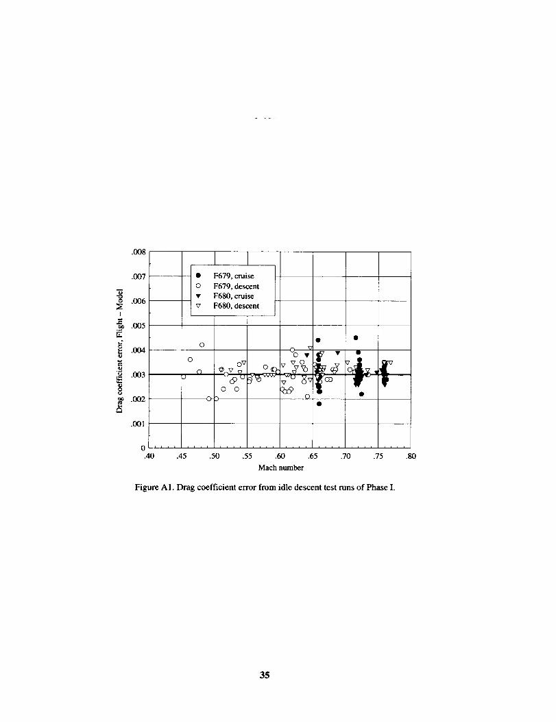
_d
I
Q
.008
.007
.006
.005
.004
.003
.002
.001
• F679, cruise
o F679, descent
• F680, cruise
F680, descent
• •O
v o qP [_
O-3 0
0 ........... i i i i i i L i i i i i i , I , _ i , _
.40 .45 .50 .55 .60 .65 .70 .75 .80
Mach number
Figure AI. Drag coefficient error from idle descent test runs of Phase I.
35

1.20
1.15
1.10
1.05
1.00
.95
.90
.85
.80.40
.... I .... I .... r .... I .... I/'l'''l .... i'''
r
- • . . .
Baseline model _ _ " " " " -....
_,,_I,,,_I,,,,I .... i .... I .... I .... I,,,
.45 .50 .55 .60 .65 .70 .75
Mach number
t
.80
(a) Left engine.
1.20
1.15
1.10
1.05
1.00
.95
.90
.85
.80.40
-' '.' ' I ' ' ' ' I _ ' ' ' I .... i , , , , I l, , , I , , _ _ I , , , ,
Baseline model--/
llill,,,,l .... I .... I .... I_,,,I .... I,,,
.45 .50 .55 .60 .65 .70 .75 .80
Math number
(b) Right engine.
Figure A2. Measured EPR at idle for descents of flight 679 with baseline and revised minimum EPR models shown•
36

35000
33000
31000
29000
27000
25000
< 23000
21000
19000
17000
15000 i300
....... i I ......... I,,1!llll II
•i_• i
Baseline minimum _-_
Revised minimum _
tLa_t_tlJJJJ_Jt_lJlt
400 500
1511111111111I_TIIIIII_IIIIIII
---- - Left engine
......... Right engine
N "::""
ii_lll ......... I ......... I .........
600 700 800 900
Fuel flow, lb/hr
Figure A3. Minimum fuel flow flight 679, run 3.
37

37000 , , ,
35000
33000
31000
29000
_. 27000
25000 -N -
< 23000
21000
19000
17000
15000 J i i-200
, , i I , , , I , , , I , , , I I L L
200 400 600 800
Thrust error, Flight - Model, lb
(a) Baseline engine model.
37000
35000
33000
31000
29000
27000
25 000
_ 23000
21000
190130
170(10
15000-200
i
_ I
i i I I t i i I , i i I i i i I i l i I i i J
0 200 400 600 800
Thrust error, Flight - Model, lb
(b) Revised engine model.
Figure A4. Composite idle thrust error for all idle descent test runs.
1000
1000
38

_N_ I]11 llll III1 IIII
.... _.... :.... : .... : ......... :.... 0 _st-_g .... !......... i .... i .... i..... i....i i ; i
................................... • bag only ......................... :..........
.... : : : !..... ..... .... ......... : : _ :..... .... .... ........... : ! _ :.......... i ; i i.... .... ..... ....
15 i i .
I
'_ 1o
Q
N 5
....i.....i-_-i_,.......ir'_i_i_,i ....i....i"-{....i...._oi.....i....
.... i ....i.... i.... i........ i,::vi .... ioO'-___-_:6_'i
-i-i .....i....
.... ! .... i.... ! .... : ........ i.... i-O-! .... i ......... ".'.... i .... i .... !......... i .... ! .... i..... !....0 i i i :,© i i i i i i i i i i i i
15000 20000 25000 30000 35000
Altitude, ft
Figure A5. Descent performance modeling errors in baseline TSRV model.
39

References
1. Erzberger, Heinz; Davis, Thomas J., and Green, Steven:
Design of Center-TRACON Automation System.Machine Intelligence in Air Traffic Management,
Andre Benoit, ed., AGARD CP-538, Oct. 1993,
pp. ll-l-11-12.
2. Williams, David H.; and Green, Steven M.: Airborne
Four-Dimensional Flight Management in a lime-Based
Air Traffic Control Environment. NASA TM-4249,1991.
3. Den Braven, William: Design and Evaluation of an
Advanced Air-Ground Data-Link System for Air TrafficControl. NASA TM-103899, 1992.
4. Williams, David H.; and Green, Steven M.: Piloted Sim-
ulation of an Air-Ground Profile Negotiation Process in
a lime-Based Air Traffic Control Environment. NASATM-107748, 1993.
5. Green, Steven M.; Den Braven, William; and Williams,
David H.: Development and Evaluation of a Profile
Negotiation Process for Integrating Aircraft and Air
Traffic Control Automation. NASA TM-4360, 1993.
6. Green, Steven M.; Davis, Thomas J.; and Erzberger,Heinz: A Piloted Simulator Evaluation of a Ground-
Based 4D Descent Advisor Algorithm. AIAA Guidance,
Navigation and Control Conference--Technical Papers,
Volume 2, AIAA, Aug. 1987, pp. 1173-1180. (Avail-able as AIAA-87-2522.)
7. Davis, Thomas J.; and Green, Steven M.: Piloted Simu-
lation of a Ground-Based lime-Control Concept for Air
Traffic Control. NASA TM-101085, 1989.
8. Hunter, George; Weidner, Tara; Couluris, George;
Sorensen, John; and Bortins, Richard: CTAS Error
Sensitivity, Fuel Efficiency, and Throughput Benefits
Analysis. 96150-02 (Subcontract under FAA ContractDTAFA01-94-Y-01046 to Crown Commun., Inc.),
Seagull Technol., Inc., July 1996.
9. Couluris, G. J.; Weidner, T.; and Sorensen, J. A.: Initial
Air Traffic Management (ATM) Enhancement Potential
Benefits Analysis. 96151-01 (Subcontract under FAAContract DTFA01-96-Y-01009 to Crown Commun.,
Inc.), Seagull Technol., Inc., Sept. 1996.
10. Erzberger, Heinz: Design Principles and Algorithms for
Automated Air Traffic Management. Knowledge-Based
Functions in Aerospace Systems, AGARD-LS-200,1995.
11. Final Report of RTCA Task Force 3 Free Flight Imple-
mentation. RTCA, Inc., 1995. (Reprinted Feb. 1996.)
12. Jardin, M. R.; and Erzberger, H.: Atmospheric Data
Acquisition and Interpolation for Enhanced Trajectory-
Prediction Accuracy in the Center-TRACON Automa-
tion System. AIAA-96-0271, Jan. 1996.
13. Slattery, Rhonda; and Green, Steve: Conflict-Free Tra-
jectory Planning for Air Traffic Control Automation.
NASA TM-108790, 1994.
14. Slattery, Rhonda A.; and Zhao, Yiyuan: En-Route
Descent Trajectory Synthesis for Air Traffic Control
Automation. Proceedings of the American Control Con-
ference, June 1996, pp. 3430-3434.
15. Green, Steven M.; Goka, Tsuyoshi; and Williams, David
H.: Enabling User Preferences Through Data Exchange.
AIAA-97-3682, 1997.
16. Benjamin, Stanley G.; Bleck, Rainer; Grell, Georg; Pan,
Zaitao; Smith, Tracy Lorraine; Brown, John M.; Ramer,
James E.; Miller, Patricia A.; and Bnmdage; Kevin A.:
Aviation Forecasts From the Hybrid-B Version ofMAPS--Effects of New Vertical Coordinate and
Improved Model Physics. Fifth Conference on Aviation
Weather Systems, American Meterol. Soc., Aug. 1993,
pp. J-5--J-9.
17. Benjamin, Stanley G.; Brundage, Kevin J.; Miller,
Patricia A.; Smith, Tracy Lorraine; Grell, Georg A.;
Kim, Dongsoo; Brown, John M.; and Schlatter,
Thomas W.: The Rapid Update Cycle at NMC. Tenth
Conference on Numerical Weather Prediction, Ameri-
can Meterol. Soc., July 1994, pp. 566-568.
18. Staff of NASA Langley Research Center and Boeing
Commercial Airplane Co.: Terminal Configured Vehicle
Program--Test Facilities Guide. NASA SP-435, 1980.
19. Knox, Charles E.: Description of the Primary Flight
Display and Flight Guidance System Logic in the NASA
B-737 Transport Systems Research Vehicle. NASATM-102710, 1990.
20. Erzberger, Heinz; and Nedell, William: Design of Auto-
mated System for Management of Arrival Traffic. NASATM-102201, 1989.
21. Computer Program Functional Specifications--Multiple
Radar Data Processing. Model A4el.3, NAS-MD-320,
FAA, Aug. 1995.
22. Cashion, Patricia; Feary, M.; Smith, N.; Goka, T.;
Graham, H.; and Palmer, E.: Development and Initial
Field Evaluation of Flight Deck Procedures for Flying
CTAS Descent Clearances. Proceedings of the Eighth
International Symposium on Aviation Psychology, Vol-
ume 1, Richard S. Jensen and Lori A. Rakovan, eds.,
Assoc. of Aviation Psychologists, 1995, pp. 438-443.
40

23.Jardin,M. R.; andGreen,S. M.: Atmospheric Data
Error Analysis for the 1994 CTAS Descent Advisor Pre-
liminary Field Test. NASA/TM-1998-112228, 1998.
24. Williams, D. H.: Impact of Mismodeled Idle Engine
Performance on Calculation and Tracking of Optimal
4-D Descent Trajectories. Fifth American Control Con-
ference, Volume 2, IEEE, 1986, pp. 681-686.
41

Table1. Test Conditions for Phase I
Test Cruise Descent Descent
condition speed Mach/CAS strategy Description
li
2i
3i
4i
5i
6i
7i
lcf
2cf
3cf
lcr
2cr
3cr
Mach 0.72
Mach 0.76
220 KCAS
Mach 0.76
220 KCAS
Mach 0.72
Mach 0.72
Mach 0.72
Mach 0.76
220 KCAS
Mach 0.72
Mach 0.76
220 KCAS
0.72/280
0.76/330
/220
0.76/280
*MC/280
0.76/310
/240
0.72/280
0.76/330
/220
0.72/280
0.76/330
/220
Idle
Idle
Idle
Idle
Idle
Idle
Idle
Constrained
Constrained
Constrained
Constrained
Constrained
Constrained
Nominal, typical company profile
Fast, earliest arrival time
Slow, latest arrival time
Fast cruise, long descent at nominal CAS
Slow cruise, long descent at constant Mach
Fast descent, Mach acceleration descent
Slow descent, long TOD decelerationCondition 1 flown from FFD
Condition 2 flown from FFD
Condition 3 flown from FFD
Condition 1 flown from RFD
Condition 2 flown from RFD
Condition 3 flown from RFD
*MC is Mach at cruise altitude at 220 KCAS.
Table 2. Test Conditions for Phase II
Testcondition
la
2a
3a
lb
2b
3b
lc
2c
3c
ld
2d
3d
Speedschedule
0.72/0.72/280
0.76/0.76/240
0.76/0.76/320
0.72/0.72/280
0.76/0.76/240
0.76/0.76/320
0.72/0.72/280
0.76/0.76/240
0.76/0.76/320
0.72;0.72/280
0.76/0.76/240
0.76/0.76/320
Automation levelpilot procedure
Conventional
non-FMS
Conventional FMS
FMS with
CTAS TOD
Range-altitude arc
Lateral
guidance
VOR/DME
LNAV
LNAV
LNAV
Verticalguidance
Mrspeed with CTASTOD
FMS with
VNAV TOD
FMS with
CTAS TOD
Range-altitude arcwith CTAS TOD
Flightdeck
FFD
RFD
RFD
RFD
42

Flight
R678
R679
R680
R681A
R681B
R682A
R682B
Date(l.rrc)
10/24/92
10126/92
10/26/92
10/27/92
10/27/92
Run
Table 3. Phase I Test Runs
Test condition Hight Metering
(table 1) deck fix
li2i3i
7i
5i6i4i3i
5i
li6i4i7i
lc2c
3clc2c3c
lc2c3c2c
3clc2c
FFDRFDRFD
RFD
RFDRFDRFDRFD
RFD
RFDRFDRFDRFD
RFDRFD
RFDFFDFFDFFD
RFDRFDFFDFFD
RFDFFDRFD
Arrival
time,UTC
Comments
KEANN 20:09:48 Day flight with good weatherKEANN 20:50:04KEANN 21:26:10
KEANN 4:38:40
KEANNKEANNKEANNKEANN
KEANN
KEANNKEANNKEANNKEANN
5:14:495:50:246:23:506:56:05
2:50:32
3:25:364:04:264:38:555:09:46
Night flight with strong jet streamwinds
Run 1 excluded from analysis
Night flight with strong jet stream
winds and pronounced wind gradient
KEANN 18:22:44 Day flight with good weatherKEANN 18:57:11
KEANN 20:54:57 Day flight with good weatherKEANN 21:31:19KEANN 22:09:08KEANN 22:43:26
KEANN 18:27:13 Day flight with good weatherKEANN 19:01:36KEANN 19:34:16 Run 3 excluded from analysisKEANN 20:05:54 Run 4 excluded from analysis
KEANN 22:08:40 Day flight with good weatherKEANN 22:46:35KEANN 23:37:36
43

Date
Flight (UTC)
R728 9116/94
R729A 9117194
R729B 9/17/94
9/18/94
R730A 9/19/94
R730B 9/19/94
R731 9120/94
9_1/94
R732 9/21/94
R733 9/22/94
*n/a means not any.
Run
234
1
2345
678910
12345
6
2345
Test condition
(table 2)
lb
lblc
2a
2a
3alald
2b2c3d3d3a
3b2a2d3c2d
3dld
lblclc3d
3b3c2b2c
2c
la2b2d
Table 4. Phase 11Test Runs
Flightdeck
RFD
RFDRFD
FFD
FFDFFDFFDRFD
RFDRFDRFDRFDFFD
RFDFFDRFDRFDRFD
RFDRFD
RFDRFDRFDRFD
RFDRFDRFDRFD
RFDFFDRFDRFD
Meteringfix
DRAKO
DRAKODRAKOKEANN
DRAKO
DRAKODRAKODRAKODRAKO
DRAKODRAKODRAKODRAKODRAKO
DRAKODRAKODRAKODRAKODRAKO
KEANN
DRAKODRAKO
KEANN
DRAKODRAKODRAKODRAKO
DRAKODRAKODRAKODRAKO
KEANN
DRAKODRAKODRAKODRAKO
Arrival
time,
UTC
*n/a
18:16:2118:56:23
n/a
n]a
17:47:0318:19:4318:53:2619:30:11
22:12:5422:49:04
n/a23:43:18
0:14:31
17:27:3018:02:0018:37:5419:13:1419:48:26
nla
n/a22:50:40
n/a
0:04:50rga1:08:351:41:33
17:27:2518:03:2018:44:31
rda
n]a
18:27:3619:01:4319:36:4120:11:12
Comments
Day flight with good weatherRun 1 aborted
Run 4 weather data only
Day flight with good weatherRun 1 aborted
Day flight with good weather
Run 8 aborted
Day flight with convective buildups
Day flight with convective buildupsRun 6 weather data onlyRun 7 aborted
Day flight with good weather
Run 1 weather data only
Run 3 aborted
Day flight with strong frontal passage
Run 4 aborted
Day flight with good weather and
strong winds aloft
Run 1 weather data only
Flown without autopilotAccelerate to 300 knots in descent
44

Table5.RadarTrackingErrors
(a)RadartrackingerrorsatCTASinitialconditionsforunacceleratedflight
Error
Ground speed, knots ......
Track angle, deg .........Position, n.mi ............
Along-trackDistance, n.mi ..........
Time, sec .............
Cross track, n.mi .........
Mean
-1.6
3.0
0.65
Std. dev.
6.5
5.0
0.34
Mean
5.0
0.14
0.98
0.62
5.9
0.10
Phase I
0.35
3.1
0.14
0.94
7.2
0.18
Phase II
Std. dev.
4.3
2.570.42
0.42
3.2
0.19
(b) Radar tracking errors at metering fix crossing conditions for deceleration segments
Error
Ground speed, knots ......
Track angle, deg .........
Position, n.mi ............
Along-trackDistance, n.mi ..........
Time, sec .............
Cross track, n.mi .........
Mean
-32.2
2.9
0.44
0.38
4.3
0.05
Phase I
Std. dev.
24.6
3.4
0.24
0.27
3.0
0.18
Phase II
Mean Std. dev.
-38.5 24.2
2.4 4.1
0.67 0.42
0.63 0.29
6.9 3.1
0.15 0.10
45

Table 6. Radar Track Position Error Statistics for Phase II blights
Elapsed Along-track error Cross-track error
Flight flight time,hr:min:sec Mean, n.mi. Std. dev., n.mi. Mean, sec Std. dev, sec Mean, n.mi. Std. dev., n.mi.
728
729a/b
730a/b
731
732
733
2:14:00
5:05:36
3:28:00
2:19:36
2:07:24
1:34:36
0.684
0.777
0.688
0.731
0.719
0.703
0.396
0.398
0.399
0.390
0.384
0.382
5.9
6.8
6.1
6.3
6.3
6.2
3.4
3.5
3.5
3.2
3.3
3.4
--0.024
0.008
0.006
--0.044
--0.037
-0.028
0.199
0.248
0.277
0.207
0.197
0.207
Total .... 16:49:12 0.717 0.392 6.3 3.4 -0.020 0.223
Table 7. Radar Track Ground Speed and Track Angle Errors for Phase II
Flight Segments
Ground speed error, knots Track angle error, degSegment
Mean Std. dev. Mean Std. dev.
Level flight 2.3 12.3 0.1 4.6
Altitude change -2.3 12.9 0.7 5.1
Turn 37.0 58.9 4.9 27.8
Postturn 56.4 55.8 5.0 12.9
Table 8. Mean and Standard Deviation Errors in Pilot Adherence to CTAS Descent Speed Schedule
Speed
Cruise MachDescent Mach
Descent CAS, knots
PhaseI
FFD
Mean Std. dev.
0.005 0.009
0.008 0.007-0.9 3.4
Phase II
RFD
Mean Std. dev.
0.001 0.0030.001 0.009
-0.2 3.1
FFD
Mean Std. dev.
0.010 0.0070.009 0.0081.5 5.5
RFD
Mean Std. dev.
0.001 0.0040.004 0.0080.3 4.8
46

Table 9. Top of Descent Errors From Phase II
Procedure
Non-FMSFMS TODCTAS TODND arcAll runs
TOD error, n.mi.
Mean
1.22.51.00.51.4
Std. dev.
1.02.80.90.41.7
All procedures using CTAS TOD* 0.9 0.8
*Includes non-FMS, CTAS TOD, and ND arc.
Table 10. Arrival Time Errors (Actual - Predicted) at Metering Fixfor Phase I
Procedure
Idle descentRFD constrainedFFD constrainedAll runs
Arrival time error, sec
Mean
16.69.9
16.414.7
Std. dev.
9.9
6.414.89.6
Table 11. Arrival Time Errors (Actual - CTAS predicted)
at Metering Fix for Phase II
Procedure
Non-FMSFMS TODCTAS TODND arcAll runs
Arrival time error, sec
Mean
1.9-4.6-9.9
2.3-2.7
Std. dev.
8.7
13.910.213.812.3
47

Table12.Arrival Time Errors (Actual - FMS predicted)
at Metering Fix for Phase II
ProcedureArrival time error, see
Mean Std. dev.
FMS TOD 2.0 11.3CTAS TOD 2.8 4.4
Table 13. Combinations of Airplane Performance and Weather Models Used in Sensitivity Analysisof Phase I Idle Descents
Set name Performance model Weather model
Baseline Boeing 737-100 CTAS MAPSRevised performance TSRV CTAS MAPSRevised weather Boeing 737-100 Flight measuredRevised both TSRV Flight measured
Table 14. Arrival Time Error Resulting From ModelingErrors in Phase I Idle Descents
Model parameter
PerformanceWeatherBoth
Time error, see
Mean
5.012.116.8
Std. dev.
1.58.89.6
48

12 °
magnetic variation
I Nmag
AKO
i I I I I I
0 5On.mL
Figure 1. Flight test area for Phase I.
OCS
............I_ _ emR _
BFF
12 °magnetic variation
o°.°*--°.
°°Nmag ..
__.:: IP 2
_.. : ..." .t" Sl_'I_
DEN 0 50n.mi.
Figure 2. Flight test area for Phase II.
49

Figure 3. TSRV Boeing 737-100 test airplane.
L-89-12405
L-80-2580
Figure 4. Research flightdeck (RFD)locafionin TSRV airplane.
50

PFD
/: ND
Figure 5. TSRV research flight deck.
L-90-13735
Display area <
Function and
mode keys
Numeric keys --_
i>ACT RTE LEGS 2/3 "
229 - _gr_ 1---I\1 1
PONNY 26_/ 31000
227 • 52rm r"--%
SMITY 2BO/ _S803
226 " 24_q2'0/ 16472
KEAI',TN224 * 19_
SWEET 210/11000A r'-I
197 • ll_
ALTUR 170/ 7200 r'-'l
<INDEXRTA SWEET ....... r--iN
-- Line select keys
Figure 6. TSRV control display unit (CDU).
51

TRK[_MAG
BOD >,_
Along-path .Iintercept point
20 OULL
TOD
Figure 7. TSRV navigation map display showing range-altitude arc and intercept point.
MODE CONTROL PANEL
330001
L_(_ V_L A"TC_VS C_ _S
TEST
[H_R IIVEhTII_EI °'" "'"'P_THIIP_HIIPA_HI_ T.,(_)
Figure 8. TSRV mode control panel (MCP).
52

ii!ii_iiii_iiii_iiiiiiiiiii_ii_i_iii_iiiii:iii:iiiii_iiii
:iiiiiiiiiiii_i!iiiii!ii!iiiii_ii:ii_i!!iiiii_ii_ii_iiii
_iiiiiiiiiiiiiiiiiiiiiii!iiii_iiiiiii!!iiiii!i!'iiiiii_i
VHF "test"communications
Management DA TestCoordinator Engineer
!iii!iiii_i_!_i!!i_ii:ii!i_i!!i_i_jii_!!iii!!i_i!!i_i!!;i!iiiiiiii!i!i!iii
i_i_iiii_iii_i_iii_i_!i_i_i_ii_i_ii_ii!iii_i!_iiiii_i_iii!ii_ii_i__iii_ii_iiiiii_iHiii!_iiiiiiiii_i_ii_iiiiii_iii_iiiiiiiiiiiiiii_iiii_iiiiiiiii
Normal ATC VHF(pilot (-_ controller)
communications
DController
Figure 9. Experimental setup at Denver Center.
53
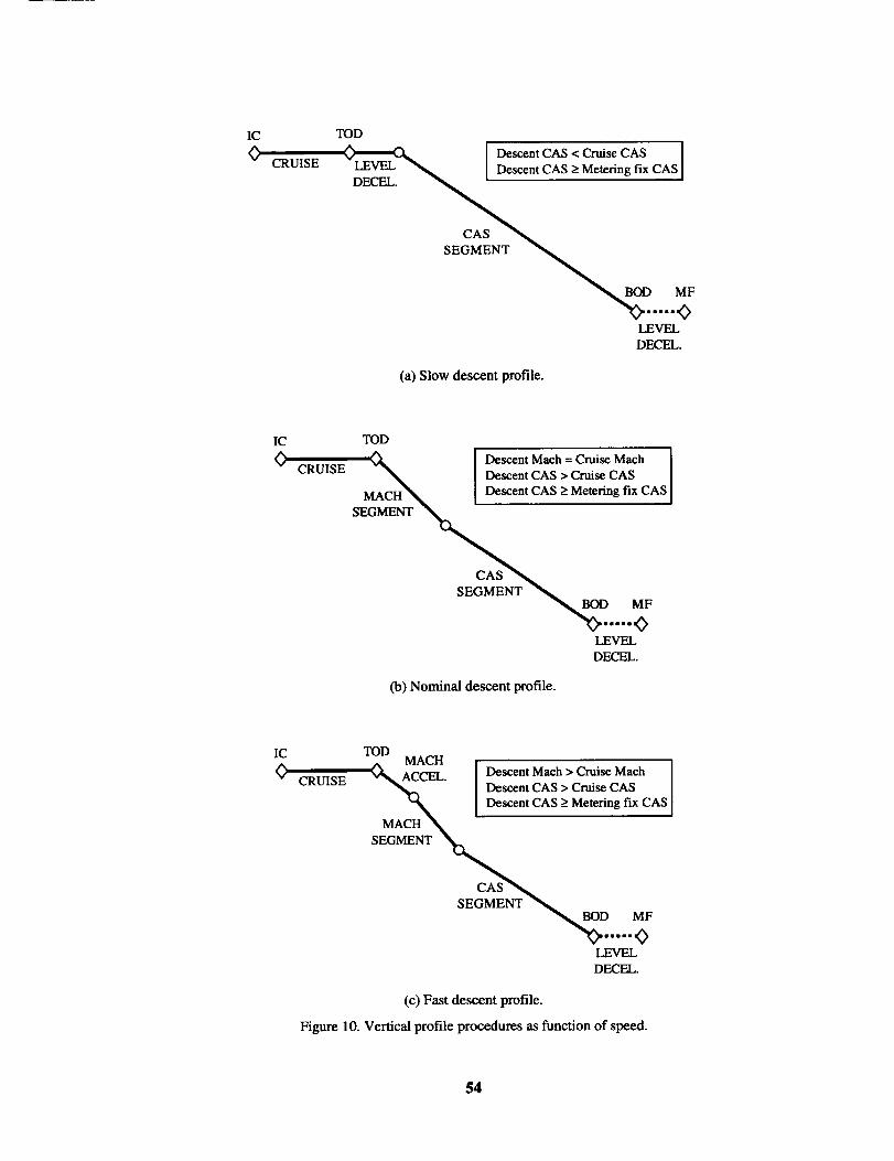
IC
CRUISE
TOD
[ Descent CAS < Cruise CAS [
LEVEL "_ [ Descent CAS _>Metering fLX CAS I
DF_L-'EL.
CAS
SEGMENT
-_. ....;_LEVEL
DECEL.
(a) Slow descent profile.
IC
0CRUISE
TOD
(_ [ Descent Math = Cruise Mach
I Descent CAS > Cruise CAS
S MACH_EGMENT_" ,I Descent CAS> Metering fix CAS
CAS "_SEGMENT "_
-,_D....;_LEVEL
D_EL.
(b) Nominal descent profile.
IC
CRUISE
TOD_ MACH .
(_ ACCEL [ Descent Mach > Cruise Math I
" I Descent CAS > Cruise CAS [
"N IDescentCAS_,Metering_ CASIMACH
SEGMENT _
CAS "_SEGMENT
,,,g_.....;FLEVEL
DECEL.
(c) Fast descent profile.
Figure 10. Vertical profile procedures as function of speed.
54

I RFD Procedure: VNAV Using FMS TOD [i
3. 10 n.mi. from TOD: 4. At FMS TOD:
[= _nga_ a._e_o-_e I [. Vhrot'_c_ime• Select CDU DESCENT page. • Set MCP CAS to descent CAS.
t _t I TOD _ $. Descent Control Procedure:
-- [ Q_- _llll Maintain VERT PATH speed using
\vLEGS page.
• Enter descent speed on DESCENT page.
• Engage VERT PATH. _,
• Set MCP altitude to 17000 fL _ 6. Bottom of Descent:
• Enter CTAS DME distance as circlearoond _ [DEN VOR on FIX page. '_J • Enter Altimeter setting prior to 19000 ft.
_ • Set MCP CAS to 250.• Select VCSS prior to 18000ft.
1. Prior To CTAS Clearance: _ • Smoothly capture crossing conditions atDRAKOI
• Level at cruise altitude, on path. at test ]condition cruise Mach. I• AUTO, ALT, HOR PATH, CAS ENG. _ DRAKO
BOD _ 17000/250 KCAS
(a) Test conditions lb and 3b.
3. 10 n.mi. from TOD: 4. At FMS TOD:
• Select CDU DESCENT page. Set MCP CAS to de,seent CAS (240).
\_ [ • Maintain VERT PATH speed using
2. Following CTAS Clearance: k/I throttle and/or speed brake.
. Verify crossing conditions at DRAKO on
LEGS page.Entex descent speed on DESCENT page.
Engage VERT PATH.
Set MCP altitude to 17000 R. _ 6. Bottom of Descent:Enter CTAS DME distance as circle ammat \ I
DEN VOR on FIX _e. _l _tet Altimeter settin_ prior to 19000 ft.
\Prior To CTAS Clearance:
[ • Level at cruise altitude' on padi" at testIconditioncruise Mach.• AUTO, ALT, HOR PATH, CAS ENG. _ DRAKO
-- 17000/240 KCAS
(b) Test condition 2b.
Figure 11. Test cards for Phase II descent using conventional FMS.
55

iRFD Procedure: VNAV Using CTAS TOD _I
3. 10 n.mi. from DME arc: 4. At DME arc:
• Ensage FPA mode. [
• Set MCP altitude to 17000 fL •
• Disengage autothrottlc. •
• Select CDU DESCENT page. •
C__ DM_j/_ TOD •
2. Folio AS Clearance •
LEGS page. '_Enter descent speed on DESCENT page.Ente¢ CI'AS DME distance as circle around
-- DEN VOR on FIX page. •
Prior To CTAS Clearance: _ •
I m Level at cruise altitude, on path, at test Icondition cruise Math. I• AUTO, ALT, HOR PATH, CAS ENG.
Set FPA to -1.5 deg. iThrottle to maintain descent Mach. ISet MCP CAS to descent CAS.
5. Descent Control Procedure:
Adjust throttle to maintain descent speeds.Engage VERT PATH at FMC TOD. --Reset FPA to -1.5 deg.Tlemlle to idle at VERT PATH capture.Maintain VERT PATH speed usingthrottle and/or speed brake.
6. Bottom of Descent:
Enter Altimeter setting prior to 19000 ft.Set MCP CAS to 250.
Select VCSS prior to 18000 ft.Snmothly capture crossing conditions atDRAKO.
OD_)m_m O DRAKOB 17000/250 KCAS
(a) Test conditions lc and 3c; early descent.
RFD Procedure: VNAV Using CTAS TOD i
3. 10 n.mi. from DME arc:
• Engage FPA mode.• Set MCP altitude to 170G0 ft.
• Disengage autothrottle.• Select CDU DESCENT page.
\ /
2. Followin_ CTAS Clearance: ,,,_r. -- •
• Verify crossLn_gconditions at DRAKO on I "'\
GSpage I '"X• Enter descent speed on DESCENT page. i -x• FJlmrCTAS DME distanceascirdc _ [ "_k
DEN VOR on FIX pag0. I N •:
L Prior To CTAS Clearance: _ •
• Level at cruise altitude, on path, at testcondition cruise Mach.
• AU'I_, ALT, HOR PATH, CAS ENG.
4. At DME arc:
• Set FPA to -4 deg (-6 for Math .76).• Select VERT PATH (should ARM).• Set MCP CAS to dcscom CAS.
S. Descent Control Procedure:
Establish FPA closing on vertical path.Maintain VERT PATH speed using speedbrake.
Retract speed brake when vertical path iscap(uteri.
6. Bottom of Descent:
Enter Altirnete_ setting prior to 19000 ft.Set MCP CAS to 250.
Select VCSS prior to 18000 ft.Smoothly capture crossing conditiom atDRAKO.
_ DRAKO
BOD'_)=.==...._ 17000/250 KCAS
(b) Test conditions lc and 3c; late descent.
Figure 12. Test cards for Phase II descent using FMS with CTAS top of descent.
56

I _ Procedure: VNAV Using CTAS TOD If
4. At DME arc:3. 10 n.mi. from DME arc:
• Tlwottle to idle.
• SetMCPaltitudetolT000fl. • MalntalnAlfitudeunlilwithin5knotsof• Disengage autoChrotfle, descent CAS
• Select CDU DESCENT page. • Set FPA to -1.5 deg when at descent CAS.
t, S TOD 5. Descent Control Procedure:
_ • Engage VERT PATH when past FMC
2. Following[ CTAS Clearance: '_E- TOD and converging on vertical path. --Reset FPA to - 1 5 deg
• Verify crossing conditions at DRAKO on _ .^ _. " "_ KO on _ • Throtti__,,_.LEGS.page. -- .... ,_ • Maintain VERT PATH speedusing
• Inter ocscent spe4mon LPe,_t_r.i_t page. _, throttleand/or _ brake• EnterCTAS DME distanceascirclearound _ ........... r......
DEN VOR on FIX page.
-- _ -- '_X 6. Bottom of Descent:
1. Prior To CTAS Clearance: 'I • Eate, Altimeter setting Prior to 19000ft.
m Level at cruise altitude, on path, at test I Xconditien cruise Math. I '_ DRAKOA ........• UTO, ALT, HOR PATH, CAS ENG. [ _.3
[ 17000/240 KCAS
(c) Test conditions 2c; early descent.
Is_ Procedure: VNAV Using CTAS TOD
4. At DME are:3. 10 n.mL from DME arc:
• Throttletoidle.
• SetMCPaltltudetol7000ft. • Maintaln Altltude until within 5 knots of• Disengage autothrottie, descent CAS
• Select CDU DESCENT page. • Set FPA to -3 deg when at descent CAS.
X FMS DME_/ 5. Descent Control Procedure:
_ To____L_ .---_-_]___---GT__V _ _ • EstablishFPA closureon vc_icalpath.-- "\ [ _ _,_ • Maintain VERT PATH speed using speed
2. Followtn 8 CTAS Clearance: ""?, _ • _rak=t speed brake whea vertical path is
• Verify_,_sing_tion, atDRA_Oen I", \ "P'_"_.LF_Spage. I"A _--
• Enter descent speed on DESCENT page. I _X• EnterCTAS DME distance as circlearound [ "'_k
DEN VOR en FIX page. [ X
N. 6. Bottom of Descent:
1. Prior To CTAS Clearance: "_• Enter Altimeter setting Prior to 19000 ft.
i Level at cruise altitude, on path, at test [
i
condition cruise Math. [ _ DRAKO• AUTO ALT HOR PATH CAS ENG. I[ ]_ .......
' ' ' i 17000/240 KCAS
(d) Test conditions 2c; late descent.
Figure 12. Concluded.
57

RFD Procedure: Altitude-Range Arc[i
3. 10 n.mL from DME arc:
l i Engage FPA mode.
Set MCP altitude to 17000 ft. •
Disongage autotlwottle. •Select CDU DESCENT page. •
\t, _t TOD •
2. Followin I CTAS Clearance: ._',, •
• Verify crossing co_ndifions at DRAKO on I _ ",LEOSpage. I _ ",_
• Enter descent speed on DES_ page. I _. ".• Enter CTAS DME distanceascircle around I _ ",
DEN VOR on FIX page. I "_"[ •
1. Prior To CTAS Clearance: _ •
n evel at cruise altitude, on path, at test lcondition cruise Mach. I• AUTO, ALT, HOR PATH, CAS ENG.
4. At DME arc:
Set FPA to -4.0 deg (-6.0 for Math .76).ThroWe to idle.Set MCP CAS to descent CAS.
5. Descent Control Procedure:
Adjust FPA to maintain descont Math atidle thrust.
When CAS reaches descent CAS, AdjustFPA so that Alt/Rmage Arc crosses BOD.Maintain descent CAS using throttleand/or speed brake.
6. Bottom of Desceat:
Enter Alfimet_ setting Prior to 19000 t_.Set MCP CAS to 250.
Select VCSS prior to 18000 ft.Smoothly capture crossing conditions atDRAKO.
BOD_'=_ DRAKO
17000/250 KCAS
(a) Test conditions ld and 3d; early descent.
3. 10 n.mL from DME arc:4. At DME arc:
• Engage FPA mode. i i• Set MCP altitude to ]70_0ft. •
• _ugagc auto_le. •• Select CDU DESCENT page. •
FMS DM1
2. Foliowin_ CTAS Clearance:
• Verify cr_sing cv_tions at DRAKO onLEGS page.
• Enter descent speed on DESCENT pege.• Ente_ CTAS DME dlstance as circle around
DEN VOR on FIX page.
Set FPA to -4 deg (-6 for Mach .76). [Throttle to idle. ISet MCP CAS set to descent CAS.
/ 5. Descent Control Procedure:
• Adjust FPA to maintain descent Mach at
1. Prior To CTAS Clearance:
I m Level at cruise altitude, o_ path, at test
condition cruise Mach.
• AUTO, ALT, HOR PATH, CAS ENG.
idle thrust.
• When CAS reaches descent CAS, AdjustFPA so that Air/Range Arc crosses BOD.
• Maintain descent CAS using speed brake
-- and/or throtfle_
6. Bottom of Descent:
• Eater Altin'_a" _ting lmOt to 19000 ft.• Set MCP CAS to 250.
• Select VCSS prior to 18000 ft.• Smoothly capture crossing conditions at
DRAKO.
OR .O17000/250 KCAS
(b) Test conditions ld and 3d; late descent.
Figure 13. Test cards for Phase II descent using range-altitude arc.
58

3. 10 n.mL from DME arc: 4. At DME arc:
r•• Set MCP altitude to 17000 ft. Throttle to idle.
• Disengage autothrottle. Set MCP CAS to descemt CAS.• Select CDU DESCENT page. Maintain altitude tmtil within 5 knots of descent CAS.
X DME/FMS 5. Descent Control Procedure:
_ _ r-xTOD • Adjust FPA so that Alt/Range Arc crosses]I_" -- l _ "X..:"", _ DRAKO.
" I N Y m Maintain descent CAS using throttle• , and/or speed brake.
2. Fonowin 8 CTAS Clearance:
• Verify crossing conditions at DRAKO on _, ',LEGS page. _ ",
• Enter descent speed on DESCENT page. _',,
• Ente¢CTAS DME distance as circle around "_'\
DEN VOR on FIX page. _',, 6. Bottom of Descent:
l. Prior To CTAS Clearance: [ • Enter Altimeter setting Pfior to 19000ft.
• AUTO, ALT, HOR PATH, CAS ENG. DRAKO
17000/240 KCAS
(c) Test conditions 2d; early descent.
_ Pr_du_:_Al,tude:Range Arc _I _ ........... _ I!.......
3. 10 n.mi. from DME arc: 4. At DME arc:
• Engage FPA mode. I I• Set MCP altitude to 17000 ft. • Throttle to idle.
• Disengage autothrottle. • Set MCP CAS to descent CAS.• Select CDU DESCENT page. • Maintain altitude tmtil within 5 knots of descent CAS.
X FMS DME/ 5. Descent Control Procedure:
_k 11_ TOD _ / . Adjust FPA so that Aft/Range Arc crosses
]_" -- _ ./ DRAKO.
-- "\_ _ II Maintain de,scum CAS using speed brake
2. Followtn B CTAS Clearance: ""x X and/ortlaxmle.
• Verifycrossing conditions at DRAKO on "%LEGS page. "". X
• Enter descent speed on DESCENT page. \,_• EnterCTAS DME distance as circle around "% _k
DEN VOR on FIX page. "'".X
",L'_6. Bottom of Descent:
l. Prior To CTAS Clearance: I • Ent_r Altimeter setting Prior to 19000ft.
• Levelat cruise altitude, on path, at test "",,_"
conditkm cruise Mach.
• AUTO, ALT, HOR PATH, CAS ENG. DRAKO
17000/240 KCAS
(d) Test conditions 2d; late descent.
Figure 13. Concluded.
59

37000
310003300035000II' ' ' I I ' ' I I ' I I I I ' ' I '
I ---0-- Phase I...r'l.-- Phase I1
2300O --
21000 --
19000 -
17000 -
15000 , , , , I _ , , , I , , , , I , , , , ,-20 -15 -10 -5 0
29OOO
._ 27000
25000
,,,,i,,,,[,J,,l,,,,
' i i i l i I i _ l i i, , l , t I i
5 lO 15 20
Air temperature deviation from standard, °C
(a) Air temperature measurements.
37000
35000
33000
31000
29000
27000
25000
23000
21000
19000
17000
15000-20 -15 -10 -5 0 5 10 15 20
Air temperature difference, Flight - CTAS, °C
(b) Air temperature modeling errors.
Figure 14. Air temperature measurements and modeling errors.
6O
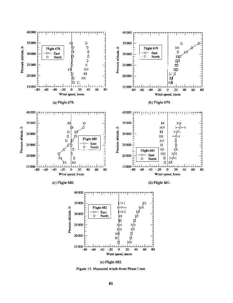
40000
35000
,i2 30000
"d
25OOO
20OOO
'''l'''l'''l''
Flight 678--<>- East
[] North
15000 ,,,I,,,1,,,1,,-80 -60 -40 -20
40000
35000
30000
25000d:
20000
15000-80
' '''1'''['''[''
t_
0
FcH
H, ,,I,,_1,,,I,,o 20 40 60
Wind speed, knots
1
80
,i
"d
40000 '''l''l['T'l ...... I'''1'''1'''
35000 __O_
Flight 679
30000 ---<>-- EastNorth
25000
20000 _ _
15000 L,,I,_,I,I,I,,, _,1,_,1,,,I,,,--80 -60 -40 -20 0 20 40 60 80
Wind speed, knots
(a) Flight 678. (b) Flight 679.
ight 680 J
"rCA_ I --0-- East
/_°io I _ N°rth
,,,I,,,I,,,],,, :,,1,,,1,,,I,
-60 -40 -20 0 20 ,10 60
Wind speed, knots
I
42
1
80
40000
350O0
30000
25000
20000
15000-80 80
,_,l,r,l,r,l,,, ,_,l,,,IT,,I ,,
Flight 681 _t3q
East _[] North
--jllJ_,,t,,,i ...... L,,,t,izl_l
-60 -40 -20 0 20 40 60
Wind speed, knots
(c) Flight 680. (d) Flight 681.
40000
35000
42 30000
._ 25000
20OOO
'''l"'l'''l"' '''l'''l'''l'''
Flight 682 ]----<3--- East-D North
llLlllJlltJlllJ_
-60
-c_
15000 ,,,It,,I,,,I,,,-80 -40 -20 0 20 40 60 80
Wind speed, knots
(e) Flight 682.
Figure 15. Measured winds from Phase I test.
61

d
.=ttl
"O
"d
4
350OO
''l'''l'''l'_'''l'''l''
30000 Flight 728--O-- East
t3 + North
25000
150001 iii I,, , I , , , I , , ,_ ,I,,iI,,,l,,
-80 -60 -40 -20 0 20 40 60
Wind speed, knots
1
80
42
35OOO
30000
25000
20000
15000-80
'''1'''1'''1'''
H
Flight 729 _C
---<)--- East
B North _c
-J,,lt,,t,Ltll,,-60 -40 -20 0
'''1'''1'''1''
,,,I,,,I,,,[,,20 40 60
Wind speed, knots
i
8O
(a) Flight 728. (b) Flight 729.
35000
30000
25000
20000
15000-80
.'"1'''1"'1'"1'"1"'1"'I"
_ _ g__ght-730
---o-- East
•n .... North
I tlt,lllltl,,,l,,,I,,,I,,,I,,
-60 -40 -20 0 20 40 60
Wind speed, knots
I
i
80
35OOO
i 30OOO
i 2500020000
-- + East ]_--'--'''l'''l'''l'''P-_ght731-] _4_2;t'l'''l'';[''lb_3q
15000-80 -60 -40 -20 0 20 40 60 80
Wind speed, knots
(c) Flight 730. (d) Flight 731.
35O0O
30000
25000
20000
15000-80
-'''1'''1'''1''' '''1'''I'''1''
Flight 732 I_
-k-od 1--<7-- East [ "t"
....northI
,,,I,,,I,,,I,,,IL,,I,,,I,,,I,,-60 --40 -20 0 20 40 60
Wind speed, knots
F_
"d
1
80
35000
30O0O
250OO
2O0OO
15000-80
'''1'''1'''1'''
H
,,,I,,,I,,,I,,
--60 ---40 -20
'''1'''1'''1''
Flight 733
East
t3 North
, ,,,I,,,I,L,I,,,
0 20 40 60 80
Wind speed, knots
(e) Flight 732. (f) Flight 733.
Figure 16. Measured winds from Phase II test.
62

"O
.0
.="d
400O0
35000
30000
25000
200O0
15OO0-80
400O0
35OO0
300OO
25OO0
200OO
150OO
--- 0 ---
-60 -40 -20 0 20 40 60 80
Wind difference, Hight - CTAS, knots
2"d
40OOO
3500O
30O00
25OOO
2000O
15000-80
,i,l,,,i,,,i,,,
-----O-- East
[] NorthTrack k
-,,,I,,,I,,,I,,,
'''['''1'''1'''
,,,1,,,I,,,I,,--60 -40 -20 0 20 40 60
Wind difference, Flight - CTAS, knots
1
80
(a) Flight 678. (b) Flight 679.
"'l'''l'''l'''l'"
Flight 680-----o--- East• [] North+ Track
'''1'''1''
W
N
q
,,,I,,,t,,-100 -80 --60 --40 -20 0 20 40
Wind difference, Flight - CTAS, knots
I
1--
60
4000O
3500O
30000
25000
20000
15000-80
- _ I--<:>--__East_ I-I [] North I:
] :
-60 --40 -20 0 20 40 60 80
Wind difference, Flight - CTAS, knots
(c) Flight 680. (d) Flight 681.
42
"d
40000
35000
30000
25000
20000
15000-80
'''l"'l'''l"'
I • I
Flight 682----O--- East
[] North------AmTrack
-_,,I,,,I,[,I,_,
'"l'"l'"l"'
MH
,,,I,,,I,,,I,,-60 --40 -20 0 20 40 60
Wind difference, Flight - CTAS, knots
1-
80
(e) Flight 682.
Figure 17. CTAS wind model errors from Phase I.
63

42
4
35OOO
3OO0O
25OOO
2OO0O
15000-80
I''' I'''1'''1_'''1''' ['''-
Flight 728
I _ EastI D North
[ _ Track
-60 --40 -20 0 20 40 60 80
Wind difference, Flight - CTAS, knots
35OOO
30000
"O
"_ 250O0
_ 2001)0
'''1'''I'''1'''
Flight 729
---o--- East
[] NorthTrack
h,,I,,,t,,,t,,,
'''1'''1'''1''
15000 t,,l,,,ll_,l,,,-80 -60 ---40 -20 0 20 40 60 80
Wind difference, Flight - CTAS, knots
(a) Flight 728. (b) Fright 729.
35OOO
30000
25000
20000
15000-80
''_1'''I'''1'''
I,,,I,,,I,,,I,,,
'''l'''i'''l''
Flight 730--<5--- East
North
Track
,_,I,,,I,,,I,,
-60 --40 -20 0 20 40 60
Wind difference, Flight - CTAS, knots
, 35000
30000
25 000
- _ 20000
, ]500080 -80 -60 -40 -20 0 20 40 60 80
Wind difference, Flight - CTAS, knots
(c) Flight 730. (d) Flight 731.
35000
30000
25000
20000
15000-80 --60 -40 -20 0 20 40 60 80
Wind difference, Flight - CTAS, knots
"O
2"d30°35o DEt73325000 _1 + Track
20000
15000 ,,1,,,I,,,I,,, ,,,1_,1,,_1,,-80 -60 -40 -20 0 20 40 60
Wind difference, Flight - CTAS, knots
1
8O
(e) Flight 732. (f) Flight 733.
Figure 18. CTAS wind model errors from Phase 1I test.
64

37000
35000
33000
m
21000 --
19000 --
17000 --
15000 a [ t [ I [ t [ t-50 -40 -30 -20 -10
31000 --
29000 --
*5 27000 ---o2
-_ 25000 -
N 23000 --
' I ' I ' I ' I '
_--O-- Eastl
i---D.. North _ _
I--A_- - Track _ \
' I ' [ ' I ' I '
L I i I J I L I L
10 20 30 40
Wind difference, Flight - CTAS, knots
(a) Phase I test.
37000
35000 -
33000 -
31000 -
' I ' I ' I ' I ' ' I ' I ' I ' I '
29000-._ 27000 -
2
25000 - _ [
23000- _
¢_ --C_ East F_
21000 - ""D North ]
19000 - + Track
17000 - _
15000 , I t [ L I , [ I I ] I [ I [ I [ I-50 --40 -30 -20 -10 0 10 20 30 40
Wind difference, Flight - CTAS, knots
(b) Phase II test.
Figure 19. Composite CTAS wind model errors.
m
m
m
50
m
m
50
65

,=
4
"d
d
4"O"d
35000
30000
25000
20000
15000-80
-'''1'''1'' 'l'''l'''l''
Flight 728
---<7-- East
o NorthTrack
iJltt,,I,, ,I,,_1,,,1_,-60 -40 -20 0 20 40 60
Wind difference, Flight - FMS, knots
I
1
80
42
35OOO
3O000
25000
20000
15000-80
'''1'''1'''1 .... ''I'''1'''1'
1-_ Flight 729
-----<7--- East[] North
-----4v--- Track
-60 -40 -20 0 20 40 60
Wind difference, Flight - FMS, knots
(a) Flight 728. (b) Flight 729.
350O0
30000
25000
20000
'''l'''l'''l"'
H
b
H_
'''l'''l'''l'''
Flight 730--<>-- East' [] North
Track
15000 ,,,I,,,I,,,I,,, ,,,I,,,I,_,t,,,-80 --60 -40 -20 0 20 40 60 80
Wind difference, Flight - FMS, knots
42
35OOO
30000 [
25000
20OO0
15000-80
'''1'''1'''1'''
H_
H
,,,1_,,I,,,I,_,
'''l'''l'''l''
731Flight
--O--- East--[q [] North
----Am Track
H
_q
-60 --40 -20 0 20 40 60
Wind difference, Flight - FMS, knots
(c) Flight 730. (d) Flight 731.
35000
30000
25000
20000
15000-80 -60 --40 -20 0 20 40 60
Wind difference, Flight - FMS, knots
_r-9-_Fr_ryr_Z_H
[
_] [ Flight 732
l East
q---I .... [] .... North----Am Track
-_
80
35000
_- 30O0O,$
2
"_ 25000
d_ 20000
15000-80
-''_l'''l''_:
I I
I 1
80
1
80
"'l'"l'"l'"
-_ Flight 733
--o-- East
North
I + Track
_qrq
Hq
-60 -40 -20 0 20 40 60 80
Wind difference, Flight - FMS, knots
(e) Flight 732. (f) Flight 733.
Figure 20. FMS wind model errors from Phase II.
66

), _ Reference VOR/DME navigation fix
/_ Fixed waypoint location DEN 046 radial
Variable location based on predicted vertical path ,-"'_1¢"
(stamng pomt)
12° FL330 -_ x__IC
magnetic vl;ation FL290 _ _ "- TODG
Nmag FL250 _ X-- FL310VFL210 _ v '-- FL270
•v _- FL230BODG -_
.t / x--FLI90
DEN _" _-- KEANN(metering fix)
v
(a) Phase I.
Denver x
CHE
(starting point) IC GOULL
4_ Reference VOR/DME navigation fix
/_ Fixed waypoint location
12 °_,, DEN 313 radial magnetic variation
", Nmag
•0_ _290 "-,F_250I ^ I ^ "I',, c_o_6_dial
FL310 FL270 \ KA_FL230 _.a
\'_/--DRAKO (meteringFL190 .._ ---_,
C_Variable location based on predicted vertical path DEN
fix)
(b) Phase II.
Figure 21. Analysis gates for trajectory comparisons.
Denver x
67

5000
o_
I
rj
-10000
-15000 --
-20 ooo --
.3-
()
• Non-FMS
• FMS TOD
A CTAS TOD
_7 ND arc
)
()
l_1_
-25 000I I I L I t i I I I
FMS predicted trajectory gate
Figure 22. Cross-track error relative to FMS path.
460
e_
450
440
430
420
410390
: i FMS reference path
Run 2
.................................. r ................. _.......... Run 3
...... Run 4
: ---- Run 10
.............. [................ i................. i _.'.'x2.:........... _:_:_._............. .,.................
.................i.................L................. .................i DRAKO i_! (metering fix)
i ........ i i t i i a d a d L i o L I ..... I .... F I F a i d a d t i i i t ..........
400 410 420 430 440 450
Denver x, n.mi.
Figure 23. Lateral paths flown during flight 729 using VOR guidance.
68

4 2_6
10
o -1
_ -2
-3
E
_ -- -[__ - .
_- __ q)
! - _
= I• Non-FMS
= • FMSTOD
: A CTAS TOD
:--- V ND arc
- I I I I I I 1 I I
FMS predicted trajectory gate
Figure 24. Distance flown error relative to FMS path.
cd<[-
I
o
O
.=<
1500
lOOO__
500
0
-500
-1000
-1500
-2000
-2500
J
ie
q
T
!q
/
• Idle descent
• Constrained descent
I)
!
I I I L I I 1
q)
)
I I
CTAS predicted trajectory gate
Figure 25. Altitude error summary from Phase I.
69

2500
2000
1500
1000
o
o -500
-1500
-2000
-2500
T
' 1
I I I I I
%2%%%%%%%%%°CTAS predicted trajectory gate
Figure 26. Altitude error relative to CTAS path from Phase 11 flight test.
2500
20O0
1500
1000
t 500
_ o
_ -500
•_ -1000
-1500
-2000
-2500
• FMS TOD .............................................................. A CTAS TOD
I t I I I t
FMS predicted trajectory gate
Figure 27. Altitude error relative to FMS path from Phase IL
7O

50
40
_D
._ 30
< 20
_ 10
o -10
_-20
-30
-50
50
• Idle descent |
f• Constrained descent
Fze
i6--
t t t
CTAS predicted trajectory gate
(a) Ground speed errors.
40
O
._ 30
< 20
I 10
o -100
-20
_ -30
--40
-50
• Idle descent
• Constrained descent
t I q T _I
7- T
I1
i i i i i i l I I I -T I
CTAS predicted trajectory gate
(b) True airspeed errors.
Figure 28. CTAS speed errors from Phase I.
71

5O
40O
30<
2o
._ 10
i°_ -10
_ -20
-30
--40
-50
• Idle descent
• Constrained descent
t I I 1
CTAS predicted trajectory gate
(c) Calibrated airspeed errors.
Figure 28. Concluded.
72

50
40
o 30
06< 20
10
g_ -10
_ -20
_ -30
-40
-50
50
7-
i
__l
t
[ iT i a r-
• Non-FMS
• FMS TOD
& CTAS TOD
_7 ND arc
- T 7-
I 1 I I I I 1 I I I
CTAS predicted trajectory gate
(a) Ground speed errors.
O
06<
4O
30
20
• Non-FMS
• FMS TOD
A CTAS TOD
V ND arc
.- ]-i 10 _ "
41 ,_-10
-20
_ -30
-40
-50I I I 1 I I I I I I I
%;'%% %%% % %% °%CTAS predicted trajectory gate
(b) True airspeed errors.
Figure 29. CTAS speed errors from Phase II.
73
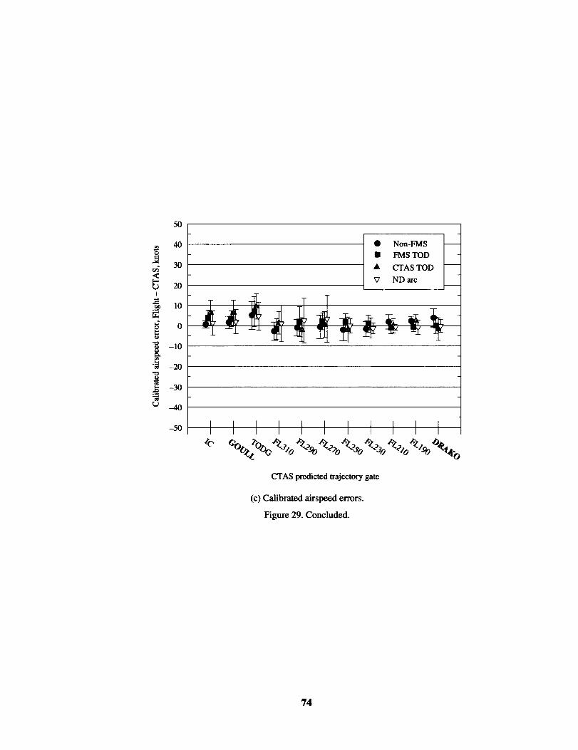
50
4Oo
30
20I
._ 10
o02
-]0
"_ -20
-30
-4O
-50
• Non-FMS
• FMS TOD
A CTAS TOD
V ND arc[
I I I I I I I l I I I
CTAS predicted trajectory gate
(c) Calibrated airspeed errors.
Figure 29. Concluded.
74

O
u_
I
¢)
50
4O
30
20
10
0
-10
-20
-30
-4O
• FMS TOD
A CTAS TOD
k k
i
-50 I
50
I I I I [ L I I I I
FMS predicted trajectory gate
(a) Ground speed errors.
I
O
_d
40
30
20
10
0
-10
-20
-30
--40
-50
• FMS TOD
A CTAS TOD
:ff_" _ _ _ _ __
!
k
I I I [ 1 I I I I I I
FMS predicted trajectory gate
(b) True airspeed errors.
Figure 30. FMS speed errors from Phase II.
75

50
o
o6
U.
I
g
40
30
20
10
0
-10
-20
-30
-40
/• FMS TOD [_
/A CTAS TOD
-50
_e
FMS predicted t_ajectory gate
(c) Calibrated airspeed errors.
Figure 30. Concluded.
76

30
25
20
15
_ 5I
._ 0
_ -5
*J -10
.._[- -15
-20
-25
-30
-- • Idle descent
• Constrained descent
-1-
---rq-
_.- .J_t_ __-1-
1|q!
-:J_ -- -J-
I I I I I I I I 1 I I I
CTAS predicted trajectory gate
Figure 31. Time error relative to CTAS path from Phase I.
30
25 :----- • Non-FMS
-- • FMS TOD20
- A CTAS TOD
¢_ 15 _:------ _7 NDarco
o4 10<
_ 5I -
o - _.
IL d.
-10
V, -15
-20
-25
q.L.._
i_ q
-30 I 1 I I J I I I I I
CTAS predicted trajectory gate
Figure 32. Time error relative to CTAS path from Phase II.
77

d
.=,<
35000 _ ! i ! i
23000:_ ......7.........
19000- ".... _'_ i i :: • FMSTOD /
17000 ......... _....... _7")•" ! .......... i.......... !" _7 NDare l
15000 .... i ........ , ............ ' .... ' ....-10 -5 0 5 10 15 20 25
Mean wind error, knots
(a) Mean along-track wind error component.
35000
33000
31000
29000
27000
25000
2300O
21000
19000
17000
150000
......... ......i . .o:o si i_ .---'f ," i • nvls'rot>
............i..........(.-_. '_!'_ .........] A cr_s'I_D
............ i ................... "" .... i ..... ".:_ .... V NDarc
............ ?............. ?.... 2._:-: , ".......... !............. _.............
: .-.---_---_---::...... i.... ..'--.,_----i .............. !.............
5 10 15 20 25
Wind error standard deviation, knots
(b) Standard deviation in along-track wind error.
Figure 33. CTAS along-track wind errors fro Phase II.
30
30
78

.=<
35000
33000
31000
29000
27000
25000
23000
21000
19000
17000
15000 '
-10
35000
....................:""_............................ - _sroD '
............................... & CTAS TOD
................,.-iA..................................................._..........I ".'
''3.
.................. _..._ .........................................................''
.................. _,_......... ._ ...................................................
-5 0 5 10 15 20 25 30
Mean wind error, knots
(a) Mean along-track wind error component.
,/"0
2
<
33000
31000
29000
27000
25000
23000
21000
19000
17000
15000
.... _--A--iV-_-I .................................. :............. _..............
:/ i........ _'A..i ' :
• : _..._ • FMS TOD............. i-;& .......... :--1 .................. A CTAS TOD
, ' /?/
.............'_......._--i........................................................
............. _.A........ ' .._ .................................................
....... A".... :-........ j..: ........................................................" ! _ i
....._-•_ ..........i........................................................
0 5 10 15 20 25 30
Wind error standard deviation, knots
(b) Standard deviation in along-track wind error.
Figure 34. FMS along-track wind errors for Phase II.
79

Form ApprovadREPORT DOCUMENTATION PAGE OMBNo.0_I_
Public reporting burden for this collection of Information is astlmated to average 1 hour per response, including the time for reviewing instructions, seerohing e0dstlng data sources,lathering and malntaIi11ng the data needed, and COml_etlng end reviewing the collso_on of Informatlon. Send comments regarding this burden estimate or any other aspect of this
_ollec1_n of information, Inducilng suggestions for reducing this burden, to Washington Headquarters Services, Dlrent(H1de for Infor_ O_ns and Reports, 1215 JeffersonDavis Hlghway, Suite 1204, Arlington, VA 22202-4302, end to the Office of Management end Budget, Paperwork Reduction Project (0704-0188), Washington, DC 20303.
I. AGENCY USE ONLY (Leeve blank) 12. REPORT DATE 3. REPORT TYPE AND DATES COVERED
I July 1998 Technical Publication4. TITLE AND SUBTITLE 5. FUNDING NUMBERS
Flight Evaluation of Center-TRACON Automation System TrajectoryPrediction Process WU 538-04-11-16
8. AUTHOR(S)
David H. Williams and Steven M. Green
7. PERFORMING ORGANIZATION NAME(S) AND ADDRESS(ES)
NASA Langley Research CenterHampton, VA 23681-2199
9. SPONSORING._IONITORING AGENCY NAME(S) AND ADDRESS(ES)
National Aeronautics and Space AdministrationWashington, DC 20546-0001
8. PERFORMING ORGANIZATION
REPORT NUMBER
L-17644
10. SPONSORING/MONITORING
AGENCY REPORT NUMBER
NASA/TP- 1998-208439
11.SUPPLEMENTARYNOTESDavid H. Williams: Langley Research Center, Hampton, VA; Steven M. Green: Ames Research Center, MoffettField, CA
12a.DISTRIBUTION/AVAILABILITYSTATEMENT
Unclassified-Unlimited
Subject Category 04 Distribution: StandardAvailability: NASA CASI (301) 621-0390
12b. DISTRIBUTION CODE
13. ABSTRACT (Maximum 200 worde)
Two flight experiments (Phase I in October 1992 and Phase II in September 1994) were conducted to evaluate theaccuracy of the Center-TRACON Automation System (CTAS) trajectory prediction process. The Transport Sys-tems Research Vehicle (TSRV) Boeing 737 based at Langley Research Center flew 57 arrival trajectories thatincluded cruise and descent segments; at the same time, descent clearance advisories from CTAS were followed.Actual trajectories of the airplane were compared with the trajectories predicted by the CTAS trajectory synthesisalgorithms and airplane Flight Management System (FMS). Trajectory prediction accuracy was evaluated over sev-eral levels of cockpit automation that ranged from a conventional cockpit to performance-based FMS vertical navi-gation (VNAV). Error sources and their magnitudes were identified and measured from the flight data. The majorsource of error during these tests was found to be the predicted winds aloft used by CTAS. The most significanteffect related to flight guidance was the cross-track and turn-overshoot errors associated with conventional VORguidance. FMS lateral navigation (LNAV) guidance significantly reduced both the cross-track and turn-overshooterror. Pilot procedures and VNAV guidance were found to significantly reduce the vertical profile errors associatedwith atmospheric and airplane performance model errors.
14.SUBJECTTERMSCTAS; FMS; Trajectory prediction; Flight management; Air traffic control
17. SECURITY CLASSIFICATION
OF REPORT
Unclassified
NSN 7540-01-280-5500
18. SECURITY CLASSIFICATIONOF THIS PAGE
Unclassified
15. NUMBER OF PAGES
8816. PRICE CODE
A05
19. SECURITY CLASSIFICATION 20. UMITATION
OF ABSTRACT OF ABSTRACT
Unclassified
Standard Form 298 (Rev. 2-89)
Prascdbed by ANSI Std. 239-18298-102