Flood Damage in the United States, 1926–2000

A Reanalysis of National Weather Service Estimates

by

Roger A. Pielke, Jr.

Mary W. Downton

J. Zoe Barnard Miller

June 2002

Environmental and Societal Impacts Group National Center for Atmospheric Research*

P.O. Box 3000, Boulder, Colorado 80307-3000

Sponsored by: Office of Global Programs National Oceanic and Atmospheric Administration

*The National Center for Atmospheric Research is sponsored by the National Science Foundation.

2

This is a report of the University Corporation for Atmospheric Research, supported by the National Science Foundation, the National Weather Service, and the National Oceanic and Atmospheric Administration, Office of Global Programs, pursuant to NOAA Award No. NA96GP0451 through a cooperative agreement. The views expressed herein are those of the authors and do not necessarily reflect the views of UCAR, the National Science Foundation, NOAA, or any of their subagencies. www.flooddamagedata.org Please cite this publication as follows: Pielke, Jr., R.A., M.W. Downton, and J.Z. Barnard Miller, 2002: Flood Damage in the United

States, 1926–2000: A Reanalysis of National Weather Service Estimates. Boulder, CO: UCAR.

Note: Present affiliation for Roger Pielke, Jr.: Center for Science and Technology Policy

Research, University of Colorado, 1333 Grandview Ave., Boulder, CO 80309-0488. E-mail: pielke@cires.colorado.edu

Cover photo credit: East Grand Forks, Minnesota, April 1997: An eerie calm settles on the water

in this East Grand Forks neighborhood. Many homes floated off their foundations, all received significant damage. Photo by David Saville, Federal Emergency Management Agency.

Limited copies of this report may be obtained upon request from: Environmental and Societal Impacts Group National Center for Atmospheric Research PO Box 3000 Boulder, CO 80307-3000 Tel: 303-497-8117 downton@ucar.edu

i

CONTENTS

ACKNOWLEDGMENTS .............................................................................................................. iii

EXECUTIVE SUMMARY .............................................................................................................v

LIST OF TABLES ......................................................................................................................... vii

LIST OF FIGURES .......................................................................................................................viii 1. INTRODUCTION .......................................................................................................................1 Why We Need Historical Flood Damage Data ....................................................................1 Sources of Historical Flood Damage Data...........................................................................2 Scope of the NWS Flood Damage Data ..............................................................................2 Purpose and Methods...........................................................................................................4 Organization.........................................................................................................................5 2. SOURCES OF FLOOD DAMAGE ESTIMATES, 1926–2000..................................................6 Overview of Historical NWS Es timates ..............................................................................6 Present Methods of Compiling Flood Damage Estimates ...................................................7 Sources of Historical NWS Estimates .................................................................................9 Additional Sources of Flood Damage Estimates ...............................................................11 Summary............................................................................................................................14 3. DEVELOPMENT OF THE DATA SETS.................................................................................15 Resolving the Data Gap, 1976–1982 .................................................................................15 Annual National Flood Damage Estimates (1926–1979, 1983–2000) ..............................16 Annual Flood Damage Estimates for the States (1955–1979, 1983–2000) .......................16 Annual Flood Damage Estimates in River Basins (1933–1975) .......................................16 Use of the Damage Estimates ............................................................................................19 4. SOURCES OF INACCURACY IN THE DAMAGE DATA ...................................................20 Clerical Errors....................................................................................................................20 Inconsistency in Reporting over Time ...............................................................................20 Low Precision of Reported Estimates ................................................................................22 Inadequate Estimation Methods.........................................................................................23 5. ACCURACY OF DAMAGE ESTIMATES..............................................................................24

Errors in Early Damage Estimates.....................................................................................24 Comparison of Damage Estimates from NWS and States .................................................30 Accuracy: Summary and Conclusions ...............................................................................40 6. DEALING WITH DATA OMISSIONS AND INCONSISTENCIES ......................................43 Frequency of Damaging Floods at the State Level............................................................43 Magnitude of Damages ......................................................................................................45 Implications for Analysis of State Damages......................................................................49 Recommendations ..............................................................................................................54

ii

7. USE AND INTERPRETATION OF NWS FLOOD DAMAGE DATA ..................................55 Analyzing Trends Over Time ............................................................................................55 Comparing States ...............................................................................................................59 Comparing Individual Flood Events ..................................................................................59 Possible Inconsistencies With Other Sources ....................................................................65 Uses of the Reanalyzed NWS Damage Estimates .............................................................65 Recommendations for Future Collection of Flood Damage Estimates .............................66 REFERENCES ..............................................................................................................................68 ABBREVIATIONS .......................................................................................................................72 APPENDIX A. Compilation of Damage Estimates for 1976–1979 .............................................73 APPENDIX B. Estimated Flood Damage, by State .....................................................................79

iii

ACKNOWLEDGMENTS This research was supported by the National Oceanic and Atmospheric Administration, Office of Global Programs (NOAA-OGP), Award No. NA96GP0451, with the able assistance of Bill Murray, Caitlin Simpson, and Rick Lawford. Additional support was provided by the U.S. Weather Research Program. The authors are particularly grateful for the assistance of Frank Richards and Joanna Dionne of the National Weather Service (NWS) Hydrologic Information Center and other NWS staff including Paul Polger and John Ogren (Silver Spring, MD) and Robert Glancy and Frank Cooper (Denver, CO). Valuable assistance and comments were received from David Wingerd, U.S. Army Corps of Engineers; Stan Changnon and Ken Kunkel, Illinois State Water Survey; Bill Cappuccio, National Flood Insurance Program (Iowa); Lisa Flax, National Ocean Service; Jacki Monday, Natural Hazards Research and Applications Information Center; Kathleen Miller, National Center for Atmospheric Research; and Tom Grazulis, The Tornado Project. Many state emergency management agencies provided information for this study. We are especially grateful to Michael Sabbaghian, California Governor’s Office of Emergency Services, for providing data and assistance related to the California 1998 El Niño disaster. Information was also provided by: Lee Helms, Alabama Emergency Management Agency Karma Hackney, Dana Owens, and Tom Mullins, California Governor’s Office of Emergency

Services Larry Lang, Colorado Water Conservation Board Yusuf Mustafa, Florida Division of Emergency Management Shirley Collins, Florida Bureau of Recovery and Mitigation, Dept. of Community Affairs Gary McConnell, Georgia Emergency Management Agency Edward Teixeira, Hawaii State Department of Defense Robert Sherman, Illinois Emergency Management Agency Phil Roberts, Indiana State Emergency Management Agency David Eash, Iowa Dept. of Natural Resources Art Jones, Louisiana Office of Emergency Preparedness Stephen J. McGrail, Massachusetts Emergency Management Agency Doran Duckworth, Michigan Dept. of State Police, Emergency Management Division Sherrill Neudahl, Minnesota Dept. of Public Safety, Division of Emergency Management Glenn Schafer and Stuart Shelstad, Minnesota Farm Service Agency Chuck May, Missouri State Emergency Management Agency Kay Phillips, Ohio Emergency Management Agency, Response and Recovery Branch Dennis Sigrist, Oregon Emergency Management Agency John Knight, South Carolina Emergency Preparedness Division Joan Peschke, Texas Emergency Management, Recovery Section Michael Cline and Harry Colestock, Virginia Dept. of Emergency Services

iv

Chuck Hagerhjelm and Terry Simmonds, Washington State Military Dept., Emergency Management Division

John Pack, West Virginia Dept. of Military Affairs and Public Safety, Emergency Services Robert J. Bezek, Wyoming Emergency Management Agency Much assistance was provided by librarians at the National Center for Atmospheric Research and the National Oceanic and Atmospheric Administration in Boulder, CO, and the staff of the U.S. Army Corps of Engineers library at Fort Belvoir, VA. Finally, special thanks to Jennifer Oxelson for constructing the website, to Roberta Klein for helpful comments on the manuscript, and to D. Jan Stewart, Anne Oman, and Jan Hopper for preparing the report for publication.

v

EXECUTIVE SUMMARY Flood damage continues to increase in the United States, despite extensive flood management efforts. To address the problem of increasing damage, accurate data are needed on costs and vulnerability associated with flooding. Unfortunately, the available records of historical flood damage do not provide the detailed information needed for policy evaluation, scientific analysis, and disaster mitigation planning. This study is a reanalysis of flood damage estimates collected by the National Weather Service (NWS) between 1925 and 2000. The NWS is the only organization that has maintained a long-term record of flood damage throughout the U.S. The NWS data are estimates of direct physical damage due to flooding that results from rainfall or snowmelt. They are obtained from diverse sources, compiled soon after each flood event, and not verified by comparison with actual expenditures. Therefore, a primary objective of the study was to examine the scope, accuracy, and consistency of the NWS damage estimates to improve the data sets and offer recommendations on how they can be appropriately used and interpreted. This report presents the following three data sets, which are also available on the World Wide Web at www.flooddamagedata.org:

• Estimated flood damage in the U.S. (1926–1979 and 1983–2000, by fiscal year; • Estimated flood damage for each state in the U.S. (1955–1979, by calendar year, and

1983–2000, by fiscal year); and • Estimated flood damage, by river basin, for the U.S. (1933–1975, by calendar year).

We found that the NWS collection and processing of flood damage data were reasonably consistent from 1934 to the present, except during the period 1976–1982. Data from NWS files and other sources made it possible to reconstruct state and national flood damage estimates for 1976–1979. However, little data was collected during 1980–1982 and large errors were discovered in estimates developed later for that period. As a result, the years 1980–1982 are excluded from the reanalyzed data sets. Evaluation of the accuracy of the estimates led to the following conclusions: 1. Individual damage estimates for small floods or for local jurisdictions within a larger flood area tend to be extremely inaccurate. When damage in a state is estimated to be less than $50 million (in 1995 dollars), estimates from NWS and other sources frequently disagree by more than a factor of two. 2. Damage estimates become more accurate at higher levels of aggregation. When damage in a state is estimated to be greater than $500 million, disagreement between estimates from NWS and other sources are relatively small (40% or less). The relatively close agreement between NWS and state estimates in years with major damage is reassuring, since the most costly floods are of greatest concern and make up a large proportion of total flood damage.

vi

3. Floods causing moderate damage are occasionally omitted, or their damage greatly underestimated, in the NWS data sets. Missing NWS estimates were discovered for floods in which the state claimed as much as $50 million damage. In summary, the NWS flood damage estimates do not represent an accurate accounting of actual costs, nor do they include all of the losses that might be attributable to flooding. Rather, they are rough estimates of direct physical damage to property, crops, and public infrastructure. Estimates for individual flood events are often quite inaccurate, but when estimates from many events are added together the errors become proportionately smaller. At the national level, these findings suggest that annual damage totals are reasonably accurate because they are sums of damage estimates from many flood events. State annual damage estimates are more problematic. Both frequency and magnitude of damage must be considered, because damaging floods do not occur every year in most states. Flood frequency cannot be determined simply by the presence or absence of a damage estimate because reporting, particularly for small floods, is unreliable. Aggregation is a key to reducing estimation errors. To compare flood damages between states, aggregate the damage estimates over many years and compare the sums. To compare damage between years, aggregate yearly state damage estimates over multi-state regions. Even when the estimates are highly aggregated, be aware that a substantial amount of variability is caused by estimation errors and interpret the results accordingly. When properly used, the reanalyzed NWS damage estimates can be a valuable tool to aid researchers and decision makers in understanding the changing character of damaging floods in the United States. Users of the reanalyzed data are advised to take the following precautions:

• To compare flood damage over time, adjust for changes in population, wealth, or development.

• To compare damage in different geographical areas, control for differences in population and in the incidence of extreme weather events during the period of study.

• Use damage estimates for individual floods with caution, recognizing that estimation errors are large. Comparison of individual floods might be better done using nominal or ordinal damage levels. Look for qualitative descriptions to compare the nature and impacts of the damage.

• Different agencies define “flood” and “flood damage” somewhat differently. Check for incompatibilities between data from different sources before seeking to combine sources or aggregate data.

The NWS damage estimates are not reliable enough to be a basis for critical decisions, such as setting flood insurance premiums or evaluating the cost-effectiveness of specific hazard mitigation measures. Better damage data are needed to evaluate the effectiveness of specific mitigation measures designed to reduce flood losses.

vii

LIST OF TABLES Table 1-1. Sources of flood damage estimates. ........................................................................ 3 Table 2-1. Published sources of flood damage estimates from the NWS and US Weather Bureau............................................................................................................10 Table 2-2. Types of flood loss reported during each era. ..........................................................12 Table 3-1. Estimated US flood damage, by fiscal year (Oct–Sep).............................................17 Table 5-1. California 1998 El Niño disaster: Estimated and actual public assistance costs, in thousands of current dollars....................................................................26 Table 5-2. Crosstabulation of flood damage estimates from the NWS and five states. Estimates are in millions of dollars..............................................................................32 Table 6-1. Comparison of damage estimates by state, 1995–1978 and 1983–1999..................47 Table 6-2. Levels of annual state flood damage in three states during all years, 1955–1978 and 1983–1999. ....................................................................................50 Table 7-1. Minnesota flood damage expenditures in major flood years 1993 and 1997 (in millions of dollars)...........................................................................................64

viii

LIST OF FIGURES Figure 5-1. Estimated flood damage in California counties in the 1998 El Niño disaster,

compared with actual costs as of June 1, 2001: (a) Initial damage estimate ..............................................................................................28 (b) Preliminary damage assessment..................................................................................29 Figure 5-2. Comparison of National Weather Service flood damage estimates with

estimates obtained from five states: (a) California, 1955–1977 ..............................................................................................34 (b) California, 1978–1998 ..............................................................................................35 (c) Colorado, 1955–1998 ..............................................................................................36 (d) Michigan, 1975–1998 ..............................................................................................37 (e) Virginia, 1977–1998 .................................................................................................38 (f) Wisconsin, 1973–1993...............................................................................................39 Figure 5-3. Scatterplot of National Weather Service flood damage estimates versus

estimates obtained from five states, in millions of 1995 dollars...........................................41 Figure 6-1. Frequency distributions of annual state flood damages (1995 dollars), 1955–1978 and 1983–1999. ..........................................................................................44 Figure 6-2. States ranked by estimated total damage during 1955–1978 and 1983–1999. ..........................................................................................46 Figure 6-3. Historical flood damage in states representing different levels of vulnerability: (a) High vulnerability, California ......................................................................................51 (b) Medium vulnerability, Alabama .................................................................................52 (c) Low vulnerability, Maine ...........................................................................................53 Figure 7-1. Estimated annual flood damage in the United States, 1934–1999: (a) Total flood damage ...................................................................................................56 (b) Flood damage per capita ..........................................................................................57 (c) Flood damage per million dollars of tangible wealth. ....................................................58 Figure 7-2. States ranked based on total flood damage (a) during 1955–1978 .....................................................................................................60 (b) during 1983–1999.....................................................................................................61 Figure 7-3. States ranked based on average annual flood damage per capita, 1983–1999.....................................................................................................................62

1

1. INTRODUCTION

A. Why We Need Historical Flood Damage Data The National Weather Service (NWS) estimates that flooding caused approximately $50 billion damage in the U.S. in the 1990s (NWS-HIC 2001). Although flood damage fluctuates greatly from year to year, estimates indicate that there has been an increasing trend over the past century (Pielke and Downton 2000). Some have speculated that the trend is indicative of a change in climate (e.g., Hamburger 1997), some blame population growth and development (e.g, Kerwin and Verrengia 1997), others place the blame on federal policies (e.g., Coyle 1993), and still others suggest that the trend distracts from the larger success of the nation’s flood policies (e.g, Labaton 1993). To understand increasing damage and assess implications for policy, decision makers need to resolve the independent and interdependent influences of climate, population growth and development, and policy on trends in damage. Increased flood damage due to changing climate requires different policy actions than would damage increases due to implementation of flood policies. The available records of historical flood damage are inadequate for policy evaluation, scientific analysis, and disaster mitigation planning. There are no uniform guidelines for estimating flood losses, and there is no central clearinghouse to collect, evaluate, and report flood damage. The data that exist are rough approximations, compiled by the NWS from damage estimates that are reported in many different ways. Moreover, most published summaries of the damage estimates focus primarily on aggregate national damage totals. Scientists need historical flood damage data at a variety of spatial scales to analyze variations in flood damage and what contributes to them. For example, during El Niño years, southern California receives more precipitation than in the typical year. Conventional wisdom suggests that the increase in precipitation should result in an increase in damaging floods. If California’s emergency planners knew this to be the case, they could prepare for the floods that come with El Niño, possibly reducing damage. In this case, scientists looking for a causal relationship would want to determine to what degree historical high damage years in southern California are associated with El Niño events. This requires sub-state-level data sets, rather than a national data set. Social scientists looking at the effect of policies designed to reduce flood damage also need access to historical data at regional and local scales. Take the example of the National Flood Insurance Program, created in 1968 to “assist in reducing damage caused by floods” (42 U.S.C. § 4102 (c)(3)). Researchers evaluating the program would like to isolate the effect of the program from all other factors influencing flood damage in particular areas. At the river basin or community level, the effect of a federal policy implemented in 1968 might be isolated and measured.

In sum, historical damage data are essential for any study that seeks to understand the role that climate, population growth and development, and policy play in determining trends in flood damage. Some studies might require data at the national level, and others at the state or

2

local level. Moreover, researchers need guidance to use the data effectively. Some data sets are not accurate enough for certain types of analysis. B. Sources of Historical Flood Damage Data Ideally, a national database of historical flood damage should cover the entire country over a long time period, using consistent criteria and methods in all times and places. Table 1-1 compares possible sources of damage data. The National Weather Service is the only organization that has maintained a long-term and fairly comprehensive record of flood damage throughout the U.S. Insurance company records include only insured property. Records of the Federal Emergency Management Agency (FEMA) include only property that qualifies for federal assistance in presidentially declared disasters. Few state and local governments maintain damage records beyond those required by FEMA. Only in newspaper archives from cities and towns across the nation might one find more complete reporting of historical flood damage. Indeed, a newspaper archive could be the best source of information on flood damage in a particular locale. But the parochial nature of such data makes aggregation problematic. For long-term coverage of the entire nation, and of most states, the NWS data sets appear to be the best available source of flood damage estimates. However, the scope, accuracy and consistency of the data must be evaluated to determine how they can be appropriately used and interpreted. C. Scope of the NWS Flood Damage Data The NWS Hydrologic Information Center (NWS-HIC 2001) describes the data as “loss estimates for significant flooding events,” providing estimates of “direct damages due to flooding that results from rainfall and/or snowmelt.” However, key concepts such as “flood” and “flood loss” are defined differently by various agencies and researchers depending on their objectives. Appropriate use of NWS damage data requires understanding of what is and is not included. Types of Flooding Ward (1990) defines a flood broadly as “a body of water which rises to overflow land which is not normally submerged.” This definition covers river and coastal flooding, rainwater flooding on level surfaces and low-gradient slopes, flooding in shallow depressions which is caused by water-table rise, and flooding caused by the backing-up or overflow of artificial drainage systems. The NWS includes damage from most types of flooding listed above, but excludes ocean floods caused by severe wind (storm surge) or tectonic activity (tsunami). These are excluded because, although they result in water inundation, they are not hydrometeorological events. In addition, the NWS excludes damage that results from mudslides because, though they are caused by excess precipitation, they are considered primarily a geologic hazard.

3

Table 1-1. Sources of flood damage estimates.

Source Timespan Spatial Scale Scope

National Weather Service flood damage data sets

1925–present Nation State Basin

Estimates of direct physical damage from significant flooding events that result from rainfall or snowmelt

Insurance records (National Flood Insurance Program, private insurers)

1969–present Nation Community

Personal property claims made by individuals holding flood insurance

Disaster assistance records (Federal Emergency Management Agency)

1992–present Nation State

Federal and state outlays for public assistance, individual assistance, and temporary housing in presidentially declared disasters

State and local government records

Varies State Varies

Newspaper archives Varies Community Varies

4

Definition of Loss, Damage, and Damage Estimates Researchers specializing in natural hazards have expressed a need for more complete documentation of losses, including both direct and indirect costs associated with flooding (Mileti 1999; National Research Council 1999; Heinz Center 2000). Direct costs are closely connected to a flood event and the resulting physical damage. In addition to immediate losses and repair costs they include short-term costs stemming directly from the flood event, such as flood fighting, temporary housing, and administrative assistance. By contrast, indirect costs are incurred in an extended time period following a flood. They include loss of business and personal income (including permanent loss of employment), reduction in property values, increased insurance costs, loss of tax revenue, psychological trauma, and disturbance to ecosystems. They tend to be more difficult to account for than direct costs (Heinz Center 2000). The NWS describes its flood loss data as estimates of “direct damages” including, for example, loss of property and crops and costs of repairing damaged buildings, roads, and bridges. The NWS estimates have usually been restricted to direct physical damage, a subset of the losses generally considered to be direct costs. The dollar figures in the NWS damage data are estimates compiled soon after each flood event, before the actual costs of repair and replacement can be known. They are not verified by comparison with actual expenditures. The estimates are gathered from diverse sources, some who use accurate estimation methods (e.g. insurance companies) and others who do not (e.g. newspapers). Therefore, NWS damage data are best described, not as “loss data”, but as “damage estimates.” D. Purpose and Methods Objectives of this study are (1) to assemble a national database of historical flood damage based on NWS damage estimates, making it as complete and consistent as possible; (2) to describe what the estimates represent; (3) to evaluate the accuracy and consistency of the estimates; and (4) to develop guidelines for use of the data and make it widely available to users. Steps followed to achieve these objectives are described below. 1. Compilation of historical flood damage data sets. The NWS Hydrologic Information Center (NWS-HIC) is responsible for compiling and archiving flood damage estimates collected from NWS field offices throughout the U.S. Its staff members provided several data sets and access to files and publications archived in their office at Silver Spring, Maryland. This report augments published NWS data with information from NWS files and reports of other federal and state agencies. The following data sets are presented: a. Estimated flood damage in the United States (1926–1979 and 1983–2000, by fiscal year); b. Estimated flood damage for each state in the U.S. (1955–1979, by calendar year, and 1983–

2000, by fiscal year); and c. Estimated flood damage, by river basin and drainage, for the U.S. (1933–1975, by calendar

year).

5

2. Review of data collection and reporting methods used by the NWS. In interviews, staff of NWS-HIC and two NWS field offices described their data and recent data collection procedures. NWS-HIC documents and several editions of the NWS Operations Manual provided additional information on past and present procedures. This report describes the nature of the damage estimates and provides a guide to their interpretation and use. 3. Evaluation of accuracy and consistency of the damage estimates. This report critically examines criteria and methods used by the NWS in collecting past and present damage estimates to identify likely sources of inaccuracy. To understand the inaccuracy generally inherent in damage estimation, the report uses statistical comparison methods to assess a California data set containing both preliminary damage estimates and actual cost information. Then it uses similar statistical methods to compare NWS damage estimates with independent estimates from state sources to evaluate the variability in flood damage estimates. Finally, it assesses the impacts of errors and omissions on aggregated damage estimates. 4. Development of guidelines for use of the data. Evaluation results show substantial errors in many of the damage estimates. Uncertainty about the accuracy of the estimates implies that comparisons of flood damage estimates from different flood events or different locations must be undertaken with caution. The report presents examples that illustrate appropriate and inappropriate ways of using the damage data and suggests ways of reducing the impact of errors. The data and an associated Users Guide are available on the World Wide Web, at www.flooddamagedata.org. E. Organization This report is organized as follows. Section 2 describes NWS procedures for obtaining damage estimates and other sources used in compiling the reanalyzed data sets. Section 3 presents the reanalyzed data sets and explains how they were developed. Section 4 describes the types of inaccuracy users should expect in the damage estimates. Section 5 compares damage estimates from different sources and analyzes the accuracy of the estimates. Section 6 suggests ways of dealing with data omissions and inconsistencies. Section 7 provides guidance for use and interpretation of the reanalyzed data, with examples and warnings, and concludes with recommendations regarding future collection and dissemination of flood damage estimates.

6

2. SOURCES OF FLOOD DAMAGE ESTIMATES, 1926–2000 For nearly a century, the NWS and its predecessor, the U.S. Weather Bureau, have collected flood damage estimates through a nationwide system of field offices. The quality of the flood damage estimates is uneven, depending on operational constraints at particular field offices and diverse sources of damage reports. Policies and procedures for collecting and compiling the estimates have changed somewhat in the course of time. A. Overview of Historical NWS Estimates The NWS has published flood damage estimates almost annually since 1933. From 1933 to 1975, reporting units were defined by natural boundaries (river basins), which could be useful for local planning on issues such as water supply, agriculture, and flood control. In 1955, annual summaries of damage by state were added. Consistent administration, methodology, and format of the published reports suggest that these data form a reasonably homogeneous time series. From 1976 through 1979, reduction of funding led to cutbacks in the compilation of flood damage data. Data collection was consistent with prior years, but there appears to have been less checking and updating of initial damage information. Publication of annual summaries ceased. In 1980, compilation of flood damage estimates was discontinued entirely. In 1983, Congress ordered the U.S. Army Corps of Engineers (USACE) to provide annual reports of flood damage suffered in the U.S. The USACE contracted with the NWS to provide the required data. NWS estimates of flood damage in each state have been published annually since 1983 by the USACE. The NWS Hydrologic Information Center (NWS-HIC) has gradually improved its procedures for compiling and checking the damage estimates. The long-term consistency in collection of flood damage data results from its connection to weather forecasting and storm warning operations of the NWS. Since at least 1950, reports on severe storms have been submitted regularly to NWS headquarters from field offices distributed across the U.S. The reports include descriptions of severe storms and associated deaths and damage. Since 1959, these reports have been published monthly in a NOAA periodical, Storm Data, and have provided the initial information used in compiling flood damage estimates. However, the field office reports are filed soon after the storm events and receive only minimal quality control before publication, thus the damage estimates provided are preliminary and incomplete. Staff at NWS headquarters perform considerable checking and follow-up to produce final flood damage estimates. This brief overview highlights a major change in the purpose and format of the flood damage data. Before 1980, the NWS compiled damage estimates for meteorological and hydrological purposes, based on natural units such as watersheds. Annual estimates were compiled by calendar year. Since 1983, the USACE and NWS have prepared flood damage information for Congress, whose members focus on the state as a political unit. Estimates are compiled by federal fiscal year.

7

B. Present Methods of Compiling Flood Damage Estimates The staff of NWS-HIC willingly answered our questions about methods used in recent years to collect and compile damage estimates. However, none had direct experience with the methods used before 1989. They provided to us copies of their flood damage data sets and made available all of the materials in their historical archives, including publications of federal agencies, files containing flood reports submitted monthly by the NWS field offices, and notes made by former staff who compiled the data into annual reports. The NWS operates approximately 120 field offices distributed across the U.S. and its territories. Each office provides weather and hydrological forecasts for an assigned area and issues warnings during severe weather and flood events. Most offices have a Warning Coordination Meteorologist (WCM) who issues storm and flood warnings in the forecast area. The WCM is also responsible for submitting monthly reports on severe storm events to the NWS, including deaths and estimates of damage to property and crops. The descriptions, deaths, and damage estimates are published monthly in Storm Data. Compiling estimates of storm damage is a minor part of the job, receiving little attention from many WCMs (Frank Richards, NWS-HIC, personal communication, 2/16/00). Field offices differ greatly in the regularity and completeness of their damage reports. Their staff obtain damage estimates from numerous local sources, and cannot always know how those estimates were made and what is included. A meteorologist at NWS-HIC is responsible for collecting flood damage reports from all of the field offices and checking the damage estimates. NWS-HIC staff are in a good position to track damaging floods because they receive the first flood and flash flood warnings issued by all of the field offices and produce the daily National Flood Summary (NWS-HIC website under Current Flooding). They also receive monthly summaries of significant hydrological events from the field offices. Hence the meteorologist is aware of most flooding events as they occur, receives narrative descriptions monthly, and can check whether estimates are received for all severe floods. Floods that appear to involve less than $50,000 in damage are entered into the database but generally not checked for accuracy or completeness. When it appears that damage could exceed $50,000, and estimates are missing or seem unreasonable based on descriptions of weather and flood conditions, other reports (e.g. news accounts), and prior experience in compiling damage records, the meteorologist contacts the field office and asks for more information and better estimates. In practice, it is often difficult to clearly separate the estimates of damage to property and crops. Therefore, in recent years, NWS-HIC has combined the estimates of property and crop damage into a single damage estimate. In most cases, damage information is collected within three months after the flood event. It is most difficult to get the information for large floods because attention in the field office is focused on other more urgent tasks related to the event. Historically, field office personnel obtained their damage estimates primarily from newspapers (Paul Polger, NWS, pers. comm., 2/16/00). Today, however, they obtain estimates

8

through a variety of contacts in their area such as emergency managers, insurance agents, and local officials. Many offices also subscribe to a newspaper service, which allows the staff to search for any story having to do with weather. Newspapers and emergency managers are the best sources of information, according to a WCM in Boulder, Colorado (Robert Glancy, NWS, pers. comm., 8/24/01). If a flood has received a presidential disaster declaration, information can be obtained from damage assessments by Federal Emergency Management Agency (FEMA) storm survey teams that travel to the flood scene. Estimates of damage to insured property can be obtained from local insurance agents. However, the estimation process is not performed with rigorous attention to accuracy. One WCM described using the following procedure: Since the largest insurer handles about 25% of the insured property in the local area, an estimate of insured losses is obtained by getting a cost estimate from that insurer and multiplying by four (John Ogren, NWS, pers. Comm., 8/29/01). A full survey of each damaged structure does not take place; instead, in many cases a simplifying formula is used to estimate damage (John Ogren, pers. comm., 8/29/01). Crop damage estimates are obtained from U.S. Department of Agriculture (USDA) agents or from monthly “flash” reports that are compiled from claims that farmers make to USDA. Damage is calculated based on expected return on the crop: Average yield is multiplied by the number of acres damaged, the estimated percentage of the crop lost, and the expected sale price based on the market at the time of event (John Ogren, NWS, pers. comm., 8/29/01). Unlike property damage, the estimates of crop damage rely on self-reporting by farmers and permit reports to be submitted up to 60 days after the event. After a major flood event market prices often rise so that, by the time of filing, the market price claimed may be higher than the market price at the time of the flood event. Storm Data’s compilers vary widely in terms of training and expertise (Frank Richards, pers. comm., 6/27/01). NWS provides operations manuals to its staff, which explain how to collect and report flood damage. However, one compiler reports that he received most of his training from previous employees who had experience with Storm Data compilation. He was referred to NWS manuals after he had been doing the job for some time (Frank Cooper, pers. comm. 8/27/01). Instructions for estimating damage have changed in successive versions of the NWS Operations Manual. For example, the 1985 revised manual required that damage estimates be entered by checking off damage categories (though actual dollar amounts could be entered in the narrative section of a report), and specified that damage below $5,000 could be omitted or entered as zero. Furthermore, the manual stated, “Damage resulting from flash floods and floods should be reported only if it is the result of local rainfall but not if it is the result of heavy rain upstream, i.e., that which fell more than 24 to 48 hours in advance of the flooding” (NWS 1985, chap. 42, p. 14). In other words, NWS wished to collect damage estimates only for floods that were the result of localized precipitation. It is uncertain how widely this rule was followed, but it was eliminated less than a decade later. In the 1994 revised manual, instructions simply state, “Damage resulting from flash floods and floods should be reported by each office in whose county area of forecast responsibility the damage was reported.” The 1994 revision also eliminated the use of damage categories, specifying that damage estimates should be entered as

9

actual dollar amounts, rounded to three significant digits. The manual further advised, “Focus attention on providing reasonable estimates of larger events (damages greater than $100,000)” (NWS 1994, chap. 42, p. 10). The field office procedures for collecting flood damage data have some notable strengths and weaknesses. Damage estimators trained by their predecessors are likely to maintain continuity in the data sets, because the training ensures that collection methodology does not change from employee to employee. However, since the NWS operations manual is not always used for guidance, employees may overlook changes in official NWS data collection policies. C. Sources of Historical NWS Estimates The NWS and the U.S. Weather Bureau published flood reports regularly in five publications from 1918 through 2001. Table 2-1 summarizes the time periods covered and the information provided by each of these sources. In the early years, damage estimates were published only after major flood events. Annual reporting of flood damage throughout the U.S. commenced in 1933. From 1934 to 1975, the River and Flood Service published monthly flood reports and annual summaries of flood damage by river basin, first in The Monthly Weather Review and later in Climatological Data National Summary. Two formats were consistently used for the annual summaries, one during 1934–1947, the other during 1948–1975. Annual damage estimates by state for calendar years 1955–1975, and monthly damage estimates for the nation during 1925–1975, were calculated and published in later reports (NWS 1975, 1977). The 1978 annual summary issue of Climatological Data National Summary announced “Compilation of the General Summary of National Flood Events and Flood Damage Statistics has been delayed. These data will be published later.” However publication of Climatological Data National Summary ceased the following year. For several years after the demise of Climatological Data National Summary, the only published NWS records of flood damage were those included in Storm Data monthly reports. As noted above, these reports often were incomplete and received little checking. Until 1995, most damage estimates were indicated by marking a damage category. (Difficulties of using estimates based on the damage categories are discussed in Section 4.) Until the mid-1970s, the cause of damage was often listed as “heavy rain”, rather than “flood”, even when flood damage was mentioned in the description. Flood descriptions gradually became more detailed in the 1980s. In general, the flood descriptions provide ample information about precipitation and river flows, but only brief mention of damage.

10

Table 2-1. Published sources of flood damage estimates from the NWS and U.S. Weather Bureau (WB).

Publication

Years of Flood

Damage Included

Spatial Aggregation

Time Periods Summarized

Information Provided

Report of the Chief of the Weather Bureau (WB)

1918–1933

River basin Water year (Oct – Sep)

Describes large flood events. Occasionally gives flood damage estimates for individual large events. (First national flood damage total reported in 1934.)

Monthly Weather Review (WB, 1934–1949)

1933–1947

River basin Calendar year Annual summaries describe damage in major floods. Tables give estimated damage for all major river drainages.

Climatological Data, National Summary (WB, NOAA, 1950–1977)

1948–1977

River basin Calendar year Monthly summaries describe flood damage and deaths in “notable” flood events. Annual summaries through 1975 give tables of damage in major river drainages. General summaries for 1972 and 1975 also give damage by state for each calendar year since 1955 and national flood damage and deaths by month and year since 1925.

Storm Data (WB, NOAA)

1959–present

County or multi-county area

— Monthly reports on storm events sometimes give brief descriptions of damage. Estimated damage to property and crops checked off on logarithmic scale until 1994, reported in thousands of dollars since 1995.

Annual Flood Damage Report to Congress (USACE)

1983–present

State Federal fiscal year (Oct – Sep)

Annual reports describe major flood events and provide table of flood damages suffered, by state. Recent reports give 10-year summary tables of flood damage and deaths, by state.

11

In 1983, when Congress asked the USACE for annual reports of flood damage suffered, Storm Data was the only available nationwide source of damage estimates. Under contract to USACE to provide estimates, NWS-HIC compiled the limited information available. In the years that followed, methods of compiling and checking the estimates were established and gradually improved. These estimates are published annually in the U.S. Army Corps of Engineers Annual Flood Damage Report to Congress (USACE 1983–2001). In the USACE damage reports from 1983 to 1988, narrative descriptions of floods are quite brief (½ to ¾ page). Many states have no damage estimate but an asterisk (*) indicates that flooding occurred. The 1984 report explains that the table gives a summation of all major flood events but that damage estimates are unavailable for minor flood events. After 1988, the descriptions of flooding and flood damage are more detailed. Beginning in 1991, the asterisk is no longer used and there are few zero entries in the tables. It appears that considerably more record keeping and analysis has gone into damage reports since 1989. Table 2-2 lists the types of flood loss reported in each of the above publications. From 1933 to 1977, estimates were divided into several categories, separated into property and agricultural damage, compiled by river basin, and presented by calendar year. In 1983, the loss categories, spatial scale, and time period changed. Estimates were summarized by state and fiscal year. In 1993, the distinction between property and agricultural damage was eliminated. Throughout the entire period, estimates focused on direct physical damage, though some data on loss of business and wages were included before 1947. Little is known about the methods used to compile and check the estimates prior to 1980. The published reports themselves show an intent to include all parts of the United States and all types of physical damage. D. Additional Sources of Flood Damage Estimates To compile and evaluate a continuous time series of damage estimates, we supplemented the NWS estimates with comparable data from other sources. Comparable estimates should represent direct physical damage in significant flood events. Extensive information would be required to fill the 1976–1982 gap in the state and national estimates. In addition, independent estimates or cost information were needed to assess the accuracy of the estimates. Reports from many sources were used to confirm damage estimates and to provide information about specific floods. Reports by Federal Agencies and Task Forces Several federal agencies prepare reports after severe flood events, in order to study the causes of particular floods and recommend improvements in systems of flood monitoring, warning, or control. Some of these reports include descriptions of earlier floods in the community, and some provide damage estimates.

12

Table 2-2. Types of flood loss reported during each era.

Reporting Years Publications Types of Flood Loss Consistently Included

1933–1946 Monthly Weather Review

Tangible property totally or partially destroyed Prospective crops Matured crops Livestock and other movable farm property Suspension of business, including wages of employees

1947 1948–1977

Monthly Weather Review Climatological Data, National Summary

Urban Property Residential Commercial Public Rural Property Crops Livestock Other Other Property Railroads, bridges, highways, etc. Public utilities Miscellaneous Unclassified

1959–present Storm Data Property damage Crop damage

1983–1992 --------------- 1993–present

Annual Flood Damage Report to Congress

Property damage Agricultural losses --------------------- Damages suffered

13

Post-flood reports prepared by district offices of the U.S. Army Corps of Engineers (USACE) often provide fairly detailed damage estimates that are more complete than NWS estimates because they are compiled many months after the flood event. The Tennessee Valley Authority (TVA) publishes post-flood reports, similar to USACE reports, for areas of the southeastern U.S. under its jurisdiction. Post-flood reports from USGS, NOAA, and the U.S. Weather Bureau usually focus on hydrological and meteorological conditions preceding and during the flood event, with only brief mention of damage. If damage estimates are provided, often they are obtained from the NWS or the USACE. FEMA has appointed special task forces to study particular major floods and recommend mitigation measures (for example, Interagency Hazard Mitigation Teams for each state affected by the 1993 Midwest flood). Their reports often contain damage estimates. National Water Summary 1988–1989: Hydrologic Events and Floods and Droughts (USGS 1991) provides historical flood information for all fifty states through 1989. In particular, floods that are considered major historical events for each state are listed, including some damage estimates for individual floods. State Reports State government agencies occasionally publish post-flood reports after particular flood events. To obtain additional, perhaps unpublished, information, we wrote to emergency management agencies in each state, asking them to provide information about historical flood damage. Five states were able to provide long-term historical summaries of their damaging floods, and these proved invaluable for analyzing the accuracy of the NWS estimates (see Section 5). Other states sent shorter-term information which provided useful examples. Unpublished NWS Damage Information The NWS-HIC staff provided copies of their state and national flood damage data sets. These data sets included unpublished estimates for 1976–1982; however, the state and national estimates were found to be incompatible, as described in Section 3. Staff members also gave us access to the historical archives at their office in Silver Spring, MD. Two sets of files proved helpful in understanding how damage estimates were compiled in the past, and were used to supplement estimates for 1976–1982. Monthly files for 1971–1995 contain the original flood reports from field offices all over the U.S., in no particular order. (These were discontinued when electronic submission of reports began in 1996.) The reports often contain descriptions of damage, but only occasionally provide damage estimates. They do not provide a basis for computing total damage by state or river basin. Yearly files contain notes made by the people who compiled damage estimates, as well as news clippings and agency communications during the year. These are extremely helpful in developing estimates for 1976–1979, as they contain preliminary annual damage estimates with notes on when and where major floods occurred.

14

Articles on flash flood damage in 1978 and 1979, published in the journal Weatherwise (Marrero 1979, 1980), were written by José Marrero who had been responsible for collecting the flood damage data formerly published in Climatological Data, National Summary. These articles provide many of our state damage estimates for those years. E. Summary The NWS effort to collect flood damage estimates has been remarkably consistent across the nation and over long time periods, resulting in the only source of long-term national flood damage information available in the United States. Similar procedures have been used to obtain estimates from field offices throughout the country, at least since 1950 and perhaps longer. Annual summaries were compiled using consistent methodologies and published in uniform formats during two extended periods, from 1933 through 1975, and from 1983 up to the present. To create continuous time series of state and national damage estimates requires obtaining compatible estimates for the missing years, 1976–1982. It would also be desirable to base all the data on the same calendar, either fiscal years or calendar years. These tasks are addressed in Section 3. The accuracy of the damage estimates is uncertain. Methods used to obtain the estimates suggest that they are often educated guesses. For many years they came primarily from newspaper reports. Today, short cuts are often used to extrapolate from a few good sources to make an estimate for an entire community. Evaluation of the accuracy of the estimates is undertaken in Sections 4 and 5.

15

3. DEVELOPMENT OF THE DATA SETS The national data obtained from NWS consisted of annual total damage estimates for the U.S., including three territories: Puerto Rico (since 1975), the Virgin Islands (since mid-1980s), and Guam (since 1994). The state data contained annual damage estimates for each state and, in recent years, the three territories. In the national data, we subtracted estimates for the three territories from the U.S. totals to create a more uniform time series representing only the 50 states. NWS estimates were spot-checked against those from other agencies. Estimates that appeared to be extremely large or small compared to published accounts of events were examined especially closely. In individual events that received follow-up study by the USACE, more accurate estimates were sometimes available. However, except during 1976–1982, there exists no compelling reason to change the NWS estimates or defer to another agency’s estimates. Section 5 provides a quantitative assessment of uncertainty in the estimates and the implications for their effective use. With a few important exceptions, the estimates presented as a result of this project have their origins in published NWS data. Obvious clerical errors have been corrected (see Section 4). A. Resolving the Data Gap, 1976–1982 To compile a complete time series of annual estimates required finding additional flood damage estimates for the years 1976–1982. As explained in Section 2, NWS ceased publication of annual flood damage summaries after 1975. Publication of comparable damage estimates did not resume until 1983, when USACE reports made damage estimates available again at the state and national levels, but not at the river basin level. To make the state and national data sets as complete as possible, we focused on obtaining and evaluating estimates for 1976 through 1982. The NWS website (NWS-HIC 2001) included previously unpublished national flood damage estimates for 1976–1982, and an NWS spreadsheet included unpublished state estimates for that period. However, the national estimates and the state total estimates differed by large margins. An old, undocumented NWS computer printout tallied individual floods, by state, in the years 1976–1988, but we found it to be filled with errors and inconsistencies. Despite a curtailment of effort, the NWS continued to compile some damage estimates during 1976–1979, which served as a starting point for our reconstruction attempts. We were able to develop estimates for 1976–1979 based on information in the NWS files and reports from other sources, as described in Appendix A. Although we tried to reconstruct estimates for 1980–1982, there were not enough sources of information, either from NWS or other agency publications, to provide estimates for those years comparable to the data in the overall data set. Furthermore, there were some large disparities between estimates found in the NWS-HIC archives for the period 1980–1982 and damage estimates provided by states, leading us to conclude that some of the damage estimates

16

for this time period are highly unreliable (see Section 5). Therefore, estimates for 1980–1982 are not included in the reanalyzed data sets, and we judge that data published by NWS for this period is of consistently lower quality than in other years. A few general comments can be made about 1980–1982. Flood damage descriptions in Storm Data, which were sparse in previous years, became even rarer in 1980–1981. The information that does exist for the period suggests that 1980 and 1981 were extremely dry years in most parts of the country, so flood damage was probably small compared to other years (Wagner 1982, USGS 1991, notes in NWS files). On the other hand, descriptions in Storm Data suggest that flood damage rose to a higher level in 1982, perhaps close to the average level of that time. B. Annual National Flood Damage Estimates (1926–1979, 1983–2000) Since flood damage estimates for 1983 through 2000 are available only for fiscal years (October–September), it is desirable to compile the entire national flood damage data set using fiscal years. Fortunately, in its annual flood damage summary for 1975, Climatological Data National Summary (NWS 1977, vol. 13, p. 117) published national flood damage estimates by month for the years 1925 to 1975. Therefore, we were able to calculate national annual damage totals based on fiscal years for 1926–1979, creating a consistent form for the full national data set. Table 3-1 shows annual damage estimates for the United States, by fiscal year, in millions of current dollars and in millions of inflation-adjusted 1995 dollars. The implicit price deflator used to adjust for inflation is also shown in the table. C. Annual Flood Damage Estimates for the States (1955–1979, 1983–2000) Annual damage estimates for each of the 50 states are given in Appendix B. The estimates for 1955 through 1975 are taken from Climatological Data National Summary (NWS 1977, vol. 13, p. 121), and are based on calendar years. Estimates for 1976–1979 are based on our reanalysis of available data (described above), and are presented by calendar year to be consistent with the earlier data. The estimates for 1983–2000 are taken from Army Corps of Engineers Annual Damage Report to Congress (1993, 2001), and are based on fiscal years (October–September). D. Annual Flood Damage Estimates in River Basins (1933–1975) The NWS and U.S. Weather Bureau compiled annual damage estimates by river basin from 1933 through 1975, publishing them first in the Monthly Weather Review (1933–1947) and later in Climatological Data National Summary (1948–1975). To make these estimates accessible to users, we organized them by large river drainages in a uniform format for the full time period.

17

Table 3-1. Estimated U.S. Flood Damage, by Fiscal Year (Oct–Sep). Fiscal Damage Implicit Damage Year (Millions Price (Millions Current Dollars) Deflator* 1995 Dollars) 1926 9.243 — — 1927 315.187 — — 1928 88.155 — — 1929 61.700 0.12854 480. 1930 25.832 0.12385 209. 1931 2.070 0.11091 19. 1932 10.365 0.09796 106. 1933 27.366 0.09541 287. 1934 18.903 0.10071 188. 1935 123.327 0.10265 1,201. 1936 287.137 0.10377 2,767. 1937 433.339 0.10815 4,007. 1938 108.970 0.10499 1,038. 1939 13.861 0.10387 133. 1940 40.067 0.10530 381. 1941 26.092 0.11244 232. 1942 91.548 0.12120 755. 1943 220.553 0.12773 1,727. 1944 99.789 0.13058 764. 1945 159.251 0.13425 1,186. 1946 68.930 0.15056 458. 1947 281.321 0.16667 1,688. 1948 213.716 0.17615 1,213. 1949 108.586 0.17594 617. 1950 129.903 0.17788 730. 1951 1,076.687 0.19072 5,645. 1952 254.190 0.19368 1,312. 1953 121.752 0.19623 620. 1954 74.170 0.19817 374. 1955 784.672 0.20163 3,892. 1956 305.573 0.20846 1,466. 1957 352.145 0.21539 1,635. 1958 224.939 0.22059 1,020. 1959 121.281 0.22304 544. 1960 111.168 0.22620 491. 1961 147.680 0.22875 646. 1962 86.574 0.23180 373. 1963 179.496 0.23445 766. 1964 194.512 0.23792 818. 1965 1,221.903 0.24241 5,041. 1966 116.645 0.24934 468. 1967 291.823 0.25698 1,136. 1968 443.251 0.26809 1,653. 1969 889.135 0.28124 3,161. 1970 173.803 0.29623 587. 1971 323.427 0.31111 1,040. 1972 4,442.992 0.32436 13,698. 1973 1,805.284 0.34251 5,271. 1974 692.832 0.37329 1,856. 1975 1,348.834 0.40805 3,306.

18

1976 1,054.790 0.43119 2,446. 1977 988.350 0.45892 2,154. 1978 1,028.970 0.49164 2,093. 1979 3,626.030 0.53262 6,808. 1980 — 0.58145 — 1981 — 0.63578 — 1982 — 0.67533 — 1983 3,693.572 0.70214 5,260. 1984 3,540.770 0.72824 4,862. 1985 379.303 0.75117 505. 1986 5,939.994 0.76769 7,737. 1987 1,442.349 0.79083 1,824. 1988 214.297 0.81764 262. 1989 1,080.814 0.84883 1,273. 1990 1,636.366 0.88186 1,856. 1991 1,698.765 0.91397 1,859. 1992 672.635 0.93619 718. 1993 16,364.710 0.95872 17,069. 1994 1,120.149 0.97870 1,145. 1995 5,110.714 1.00000 5,111. 1996 6,121.753 1.01937 6,005. 1997 8,934.923 1.03925 8,597. 1998 2,465.048 1.05199 2,343. 1999 5,450.375 1.06677 5,109. 2000 1,336.744 1.09113 1,225. _______________ * Source: U.S. Bureau of Economic Analysis, 2001. — Data unavailable, see text for discussion.

19

The basin-level damage estimates are available in spreadsheet form from our website, www.flooddamagedata.org. Estimates are presented by calendar year. The grouping of basins within drainages is somewhat different from that commonly used to define water resources regions (e.g., U.S. Dept. of Commerce, 1978 Census of Agriculture) because, over the years, the NWS sometimes changed its groupings. We developed uniform basin definitions for the full time period by using the following organizational system:

(1) Damages are grouped by drainage (e.g, St. Lawrence Drainage, Upper Mississippi, Great Basin) starting in the eastern part of the United States and moving towards the west coast, and then alphabetically by individual or grouped river basin(s).

(2) Often, the NWS grouped individual rivers together in annual summaries. For example, damage on the White and Wabash Rivers were usually included together as one estimate. If the published sources of flood data included damage for two river basins together in one year, then data for these two (or more) rivers were added together for all other years. This was the simplest way to produce a coherent data set that could be searched and produce just one row of data for one river basin.

(3) In many of the years, damage on unnamed streams was included. If the publication did not give a stream name, damage was included in a row for the drainage called “small streams.”

(4) Sometimes the publications would include a river and its small tributaries together, by saying “X River and tributaries.” When damage was published in this format, it was entered into the database under the river itself. So, damage listed for some rivers in some years may include not just the river, but its small tributaries (such as creeks).

(5) Creeks that were included separately in NWS publications from the rivers to which they are tributaries were entered into the database separately. Creeks can be differentiated from rivers in the database because they are labeled “Cr.,” whereas rivers are entered with the river name only. An exception to this rule is for rivers with Spanish names, such as the Rio Hondo and Rio Grande. Since users may want to search for “Rio Hondo” rather than “Hondo,” “Rio” is included in the database.

(6) Users looking for damage information on rivers with branches (such as North Platte, South Platte, and Platte) should look for each of these branches. In some cases, all of the branches of one stream are included together, and in some cases they are not.

(7) Several of the streams in the data set cross drainage boundaries. If there is a question about which drainage a stream is in, a user should look in both drainages.

E. Use of the Damage Estimates Users of these data sets should be aware that there is uncertainty in the damage estimates, with a likelihood of large errors in some estimates. Types of inaccuracy are described in Section 4, and the magnitude of errors is analyzed in Section 5. In consideration of uncertainty, recommendations regarding appropriate uses of the data are offered in Sections 6 and 7.

20

4. SOURCES OF INACCURACY IN THE DAMAGE DATA Sections 4 and 5 analyze the accuracy of flood damage data received from the NWS Hydrologic Information Center. The goals are to (1) identify errors, inconsistencies, and uncertainties in the estimates, and (2) assess the accuracy of the estimates. The analyses focus on national and state annual damage estimates for the period 1955–1998. Discussions with staff and comparison of the available materials revealed several sources of inaccuracy and inconsistency in the time series of historical damage estimates: 1. Clerical errors 2. Inconsistency in reporting over time 3. Low precision of reported estimates 4. Inadequate estimation methods Each source of inaccuracy is described briefly below. Many of the clerical errors were correctable. Inconsistencies are inevitable in data collected over a long time period; their existence should be noted, but the effects are not measurable. Assessment of the inaccuracy introduced by poor estimation methods is undertaken in Section 5. A. Clerical Errors These include mistakes in data entry, transcription, and labeling. Clerical errors were found and corrected, if possible, by comparing the data sets with published sources and material in the archive files. Mistaken labeling included, for example, the statement that all damages were summed by fiscal year (Oct. – Sep.) when, in fact, the national data had been summed by calendar year (Jan. – Dec.) through 1982. B. Inconsistency in Reporting over Time Published NWS reports of flood damage are uniform in format and content for extended periods, leading us to assume that fairly consistent methods were used within the periods 1934–1979 and 1983–present (see Section 2). However, collection of flood damage data was greatly curtailed in 1980, then restarted in 1983 with a new purpose and less detailed reporting. Before 1980, the data were aggregated by river basin and calendar year with several types of flood loss itemized separately. After 1982, data were aggregated by state and fiscal year (Oct.–Sep.), at first with distinction between damage to property and crops, later with only the total of the two. The difference in data collection between the two periods introduces errors when one attempts to develop a uniform data series for the full timespan. Inconsistency in spatial units Flooding naturally occurs in river basins, not necessarily bounded by individual states. When rivers form the state lines or floods cross state lines, assigning historical losses to the proper state is problematic. Our efforts to assemble estimates for 1976–1979 shed some light on the uncertainties involved. For example, the Wabash River rises in Indiana, but it forms a part of the border between Indiana and Illinois. NWS records on floods in 1976 and 1977 did not indicate how Wabash River flood damage should be divided between Indiana and Illinois; therefore, we had to decide the allocation arbitrarily. Another example is the Pearl River, which

21

rises in Mississippi and flows through Louisiana. The NWS reported high flood losses in 1979 in the Pearl River and adjoining basins, including parts of Alabama, but we could not accurately assign the damage among the three states. It is likely that similar uncertainties existed when the NWS converted 1955–1975 river basin damage estimates into state estimates. Thus, occasional mistakes in assigning damage to particular states should be expected. Inconsistency in time periods NWS flood reports have usually been filed monthly, but aggregation periods have changed. Fiscal or calendar years are useful for accounting purposes; water years (which differ by geographic location) are more meaningful for scientific purposes. For example, NWS use of calendar years (through 1979) was problematic in aggregating data for locations along the Pacific coast. There, December – January is the peak flood season, leading to uncertainty in assigning damage to the correct year. (It appears that the NWS resolved this by assigning all the damage from a particular flood season to the year in which the hydrologic flooding peaked.) The present use of October – September fiscal years corresponds well to water years across the U.S, since fewer floods occur in the autumn dry season. Inconsistency in losses included NWS policies on what kinds of losses to include have changed somewhat over the years. Damage estimates published through 1975 focused primarily on damage to property and crops, but included some indirect losses (loss of business and wages, 1934–1947; a “miscellaneous” loss category, 1948–1975). Since 1975, estimates routinely collected for Storm Data have been labelled only as property damage and crop damage. Present policy is to focus exclusively on physical damage to property and crops (John Ogren, NWS, personal communication, 8/29/01). However, the estimates come from diverse independent sources, so other types of damage could be included occasionally. The NWS process of collecting damage data has always focused more attention on larger floods. Possible inconsistencies related to the exclusion of floods involving low damage are examined in Section 6. It is sometimes impossible to separate damage by flood and other storm-related causes (e.g. wind, hail, snow, or ice). Typically, the full amount has been labeled as flood damage if heavy rain or river flows are considered to be the primary cause. Thus, NWS flood damage estimates are sometimes inflated by including other causes. Conversely, flood damage may be omitted when the major cause of damage is wind (hurricanes, tornadoes), snow, or ice. These uncertainties have existed throughout the entire data series and sometimes lead to incompatibilities with data from other agencies. C. Low Precision of Reported Estimates The estimates have always been collected from myriad sources, differing greatly in precision and accuracy. Field office estimates sometimes include very precise figures; more often they give only one or two significant digits. Aggregated sums give a misleading impression of greater precision. For example, separate estimates of $7 million, $400,000, and $17,000 add to a more precise-looking annual estimate of $7,417,000 but the accuracy is limited by that of the largest estimate ($7 million, in this case).

22

Even one-digit accuracy is not assured. Published reports sometimes disagree greatly on the amount of damage in a particular flood event. For example, shortly after the failure of the Teton Dam in Idaho in 1976, damage estimates ranged from $400 million to $1 billion (Chadwick et al. 1976). In subsequent reports from several agencies, the $1 billion estimate was used repeatedly with no further refinement (for example, USACE Walla Walla District 1977). A final report on the Teton Dam failure (Eikenberry et al. 1980) gave the only specific figures: loss of a $102.4 million project investment and over $315 million paid to more than 7,500 claimants. This establishes a minimum loss of about $417 million, but only covers a portion of the total damage. In creating the reanalyzed data set, we chose to use the geometric mean of the minimum and maximum estimates, producing a damage estimate of $650 million. After NWS reports on flood damage were discontinued in 1980, Storm Data became the primary source of flood damage estimates (see Section 2). From 1980 until about 1984, the accuracy of available estimates is limited by Storm Data reporting procedures. At that time, NWS field offices reported damage estimates by checking categories on the following logarithmic scale: 1 Less than $50 2 $50 to $500 3 $500 to $5,000 4 $5,000 to $50,000 5 $50,000 to $500,000 6 $500,000 to $5 million 7 $5 million to $50 million 8 $50 million to $500 million 9 $500 million to $5 billion Such estimates indicated only the order of magnitude of the damage (e.g. roughly a $100,000 flood, a $1 million flood, a $10 million flood). Occasionally, more specific damage estimates were included in narrative descriptions of a flood event. To add a set of these categorical estimates, each category must be assigned a point value. Proportional errors are minimized by using the geometric mean of a category’s end points. That is, category k is from $0.5 × 10k to $5 × 10k (when k > 1), so the best estimate is

(2.5)0.5 × 10k = 1.58 × 10k.

However, the individual estimates could be in error by more than a factor of 3. For example, an event with damage originally estimated anywhere between $500,000 and $5 million would be entered into the data set as damage of $1.58 million. This is about 3 times higher than an estimate at the low end of the range, and about 1/3 of an estimate at the high end of the range. Errors associated with these logarithmic categories are of concern primarily in the 1980–1984 flood damage estimates. By 1985, it appears that NWS-HIC had instituted some follow-up checking and refinement of the estimates, at least for major floods. Use of logarithmic categories in Storm Data was discontinued in 1995. Since then, one- or two-digit estimates have been given in thousands or millions of dollars (e.g. $60K or $3.2M).

23

D. Inadequate Estimation Methods Potentially the most serious source of inaccuracy is the ad hoc approach to obtaining damage estimates from each NWS field office (described in Section 2). The estimates are collected by staff members who have little or no training in damage estimation and who rely on diverse sources. Estimation methods used by their sources are unknown, and completeness of coverage varies. Estimates are usually obtained within 2 months after a flood event and are not compared by the NWS with records of actual damage. Incomplete reports and omissions A state emergency management official (Kay Phillips, Ohio Emergency Management Agency, personal communication, 7/25/00) complains that the NWS calls her asking for a damage estimate within a few weeks after a disaster. At that time, the extent of damage is unknown and emergency managers are scurrying to respond to immediate needs. They have some knowledge of losses to individuals, but little knowledge of damage to infrastructure, which makes up a large part of total losses. Thus, in her opinion, early loss estimates tend to be much too low in relation to final tabulations. An example of underestimation is the NWS damage estimate for California flooding associated with Hurricane Kathleen in 1976. The NWS dataset (which had not been fully updated because annual summaries were discontinued that year) gave a damage estimate of $42 million, whereas estimates in subsequent published reports (e.g., Montane 1999) are 3 to 4 times higher. Errors of omission occur when a significant flood event is overlooked entirely. For example, flash floods in California in July 1979 caused damage estimated at $26–50 million (Montane 1999), but the NWS dataset reported no damage. Potential biases A substantial bias toward underestimation is expected due to incomplete reporting and omission of some floods. However, we hypothesize that some damage estimates provided to the NWS field offices might be biased upward if, for example, losses were exaggerated to improve chances of getting state or federal assistance. Accuracy and bias in early damage estimates are examined in Section 5.

24

5. ACCURACY OF DAMAGE ESTIMATES

In general, estimates of damage contain a high degree of uncertainty. Ideally, estimation errors would be measured by systematically comparing estimates with actual costs, which often are not known until long after a flood event. Unfortunately, actual cost data are seldom collected in a form that can be compared with estimates made at the time of the flood. This section examines the accuracy of flood damage estimates in two ways: (1) by comparing estimates with actual costs in one large flood disaster, and (2) by comparing pairs of estimates from different sources for many flood events. A. Errors in Early Damage Estimates

NWS flood damage estimates are usually compiled within three months after a flood event, long before the actual costs can be known. Until recently, even in serious disasters, actual total damage costs were not systematically compiled by any agency. There was no way of checking the accuracy, or even the reasonableness, of most damage estimates.

In recent years, however, FEMA has systematically collected cost data for the programs it administers – admittedly only a fraction of total disaster costs. Beginning in 1992, FEMA instituted a computerized system for recording and tracking applications for federal assistance in presidentially declared disasters. State and county governments have gradually developed the capabilities to link to this system. The damage estimates submitted by local officials to FEMA probably represent the best available early estimates under disaster conditions. A team visits each damage site to view the extent of losses and make preliminary estimates. Thus, in some disasters and some jurisdictions, it is now possible to systematically compare early damage estimates with actual costs. Data from FEMA’s Public Assistance Program are particularly appropriate for our purposes because a large portion of the losses involve physical damage to property. Public assistance covers damage to public facilities such as roads and bridges, schools, government buildings, and nonprofit agencies.

In the aftermath of a natural disaster, damage information is assembled according to guidelines established by FEMA. The following stages are described by FEMA (1998) and Michael Sabbaghian1 of the California Office of Emergency Services (OES) (personal communication 8/30/00).

(1) Initial Damage Estimate (IDE): Local officials provide estimates of physical damage

based on early reports and descriptions, without necessarily visiting the damage sites. (2) Preliminary Damage Assessment (PDA): A team including local, state, and FEMA

officials visits the damage sites to do a “windshield estimate,” perhaps viewing the sites from a car window or walking around. The PDA estimates are used to decide whether federal assistance is needed. If so, they are submitted to FEMA as part of the governor’s request for a presidential disaster declaration.

1Michael Sabbaghian, Deputy Public Assistance Officer for the California OES, manages disaster recovery activities for infrastructure and is responsible for grant management. He explained the process for estimating and recording losses in presidentially declared disasters. He also provided the damage estimates and cost data for the 1998 California El Niño disaster, which is used in this section.

25

(3) Damage Survey Report (DSR): Applicants submit requests for public assistance with detailed worksheets estimating the cost of repairs. FEMA or the state perform inspections (physical surveys) for each large project and “verify documentation on a portion of the small projects” (FEMA 1998). The DSR is used to obligate federal and state disaster assistance funds. The DSR obligations change as bids are received to accomplish the repair work, and computer records are updated accordingly.

(4) Actual Cost: Final total costs when all projects are completed and the DSR is closed. For large disasters, closure might not occur until 4 to 5 years after the disaster event.

Descriptions of the NWS procedures for obtaining flood damage estimates suggest that,

in most cases, the estimates have been qualitatively similar to the IDE and certainly no better than the PDA. Indeed, NWS field offices obtain some of their estimates from FEMA’s survey teams (Section 2). Only in the largest floods (notably, the widespread flooding of the upper Mississippi basin in 1993) have extensive efforts been made to update the damage estimates over an extended period.

Therefore, to estimate the errors in early damage estimates that can be expected under good conditions (that is, from officials who have systematically viewed the damage), we use FEMA records from a recent flood disaster as a case study. In February 1998, winter storms with heavy rains led to widespread flooding in California. The president declared a major disaster in 41 counties, designated the “1998 California El Niño” disaster (FEMA-1203-DR). Table 5-1 shows the IDE and PDA estimates for each county under the public assistance program. It also shows the funds that had been obligated in the FEMA database as of June 1, 2001. Although the DSR has not been closed at the time of this writing, it is expected that nearly all costs have been obligated; therefore we will treat these figures as the “actual costs.”

The bottom line of Table 5-1 shows that total public assistance costs in the state were approximately $316 million. The PDA underestimated the total costs by only 6% ($19 million). Because no IDE was provided for several counties, the total IDE of $240 million should be compared with the total actual cost of $279 million from the matching 33 table entries. On that basis, the IDE underestimated total costs by about 14% ($39 million).

Estimates for smaller units (individual counties and the “state agencies” category) are much less accurate, however. Errors in the IDE are particularly large, ranging from underestimation by $26 million (82%) in Los Angeles County to overestimation by $20 million (316%) in San Benito County. In the PDA, errors range from underestimation by $16 million (52%) in the state agencies category to overestimation by $23 million (304%) in San Bernardino County.

26

Table 5-1. California 1998 El Niño Disaster: Estimated and actual public assistance costs, in thousands of current dollars.

Actual IDE PDA County Cost Prop.of Prop.of (By 6/1/01) Estimate Actual Estimate Actual State Agencies 30091 7129 0.24 14497 0.48 Alameda 18471 12971 0.70 8176 0.44 Amador 258 235 0.91 176 0.68 Butte 1726 665 0.39 706 0.41 Calaveras 131 -- -- 162 1.24 Colusa 4652 25000 5.37 1829 0.39 Contra Costa 5631 3885 0.69 4760 0.85 Del Norte 271 -- -- 461 1.70 Fresno 1701 820 0.48 1052 0.62 Glenn 3802 21250 5.59 9884 2.60 Humboldt 7748 1049 0.14 1753 0.23 Kern 12312 -- -- 10306 0.84 Lake 1889 1395 0.74 3044 1.61 Los Angeles 31229 5660 0.18 35516 1.14 Marin 6449 3319 0.51 5447 0.84 Mendocino 2836 4259 1.50 3846 1.36 Merced 2327 490 0.21 734 0.32 Monterey 26182 20181 0.77 11822 0.45 Napa 468 720 1.54 448 0.96 Orange 12617 3992 0.32 16720 1.33 Riverside 3130 -- -- 5964 1.91 Sacramento 2366 -- -- 3066 1.30 San Benito 6455 26870 4.16 10595 1.64 San Bernardino 7525 -- -- 30429 4.04 San Diego 6977 -- -- 9180 1.32 San Francisco 3859 12300 3.19 3703 0.96 San Joaquin 2657 655 0.25 3155 1.19 San Luis Obispo 4006 772 0.19 4915 1.23 San Mateo 21951 16110 0.73 26328 1.20 Santa Barbara 15816 75 0.00 12954 0.82 Santa Clara 13638 9846 0.72 13310 0.98 Santa Cruz 12459 13673 1.10 6320 0.51 Solano 3346 3628 1.08 8564 2.56 Sonoma 11779 11180 0.95 4127 0.35 Stanislaus 2122 -- -- 909 0.43 Sutter 1039 1582 1.52 758 0.73 Tehama 881 20000 22.70 616 0.70 Trinity 1091 1970 1.81 975 0.89 Tulare 2149 -- -- 919 0.43 Ventura 20391 3302 0.16 14350 0.70 Yolo 909 4321 4.75 4484 4.93 Yuba 592 196 0.33 249 0.42 Total 315929 239500 0.86* 297204 0.94 ________________ * Proportion of actual cost ($279 million) of cases with an IDE.

27

Figures 5-1(a,b) show scatterplots of (a) the IDE vs. actual costs and (b) the PDA vs. actual costs. Logarithmic scales are used on the axes to highlight proportional differences between estimates and actual costs. The solid diagonal line represents perfect agreement. Data points outside of the two dashed lines are cases in which the estimate differs from the actual costs by more than a factor of two. Clearly the IDE is less accurate than the PDA: the points are much more scattered. (Correlations between the logs of estimates and actual costs are r = 0.46 for the IDE and 0.88 for the PDA.)

Since the Initial Damage Estimates are based on rather superficial damage descriptions, it is not surprising that large errors are the norm: Over half of the IDEs (18 out of 33) are off by at least a factor of two, and 13 of them are off by more than a factor of four. As a percentage of the actual costs, the IDE errors can be enormous, ranging from a 99.5% underestimate in Santa Barbara County to a 2170% overestimate in Tehama County. The Preliminary Damage Assessments are somewhat better, yet over one-third (15 out of 42) are off by at least a factor of two and 3 of them are off by more than a factor of four. The PDA errors range from a 77% underestimate in Humboldt County to a 393% overestimate in Yolo County.

The population of some California counties exceeds that of many small states. So estimation errors in the larger counties are indicative of the error levels to be expected in many states. For example, Los Angeles County, with a 1990 population of 8.9 million, is larger than 42 of the states. Table 5-1 shows that, in this disaster, the IDE underestimated actual costs by 82%.

To check for systematic bias in these early damage estimates, we used a statistical paired-comparison test. A systematic tendency to underestimate might be expected if some types of damage cannot be observed without careful inspection. On the other hand, we wondered if there might be a tendency for local officials to overestimate damage in order to increase the chance of being considered for federal aid. The IDE and PDA estimates were compared with actual costs, as follows:

Let ei = estimated damage, ai = actual cost. We wish to test the null hypothesis that the geometric mean of ei/ai = 1. This is equivalent to the hypothesis that mean[log(ei) - log(ai)] = 0. We tested the hypothesis twice, first letting ei represent the IDE values in Table 5-1 (N = 33), then letting ei represent the PDA values (N = 42). A t-test is appropriate, even in these small samples, because the sample values log(ei) – log(ai) are approximately normally distributed. For the IDE, t = –1.27, and for the PDA, t = –1.10, neither of which is statistically significant at a 95% confidence level. Though there may be a tendency to underestimate the amount of damage, the bias is not statistically significant.

In summary, this example indicates that positive and negative estimation errors tend to

average out when estimates are highly aggregated in a large flood event (over $300 million damage in 1998 dollars, in this case). The initial rough estimates (IDE) tended to underestimate actual damage and the more careful PDA estimates were reasonably accurate. It shows, however, that in smaller flood events ($30 million damage or less in 1998 dollars), which involve substantially less aggregation, the errors can be extremely large. Half of the PDA estimates

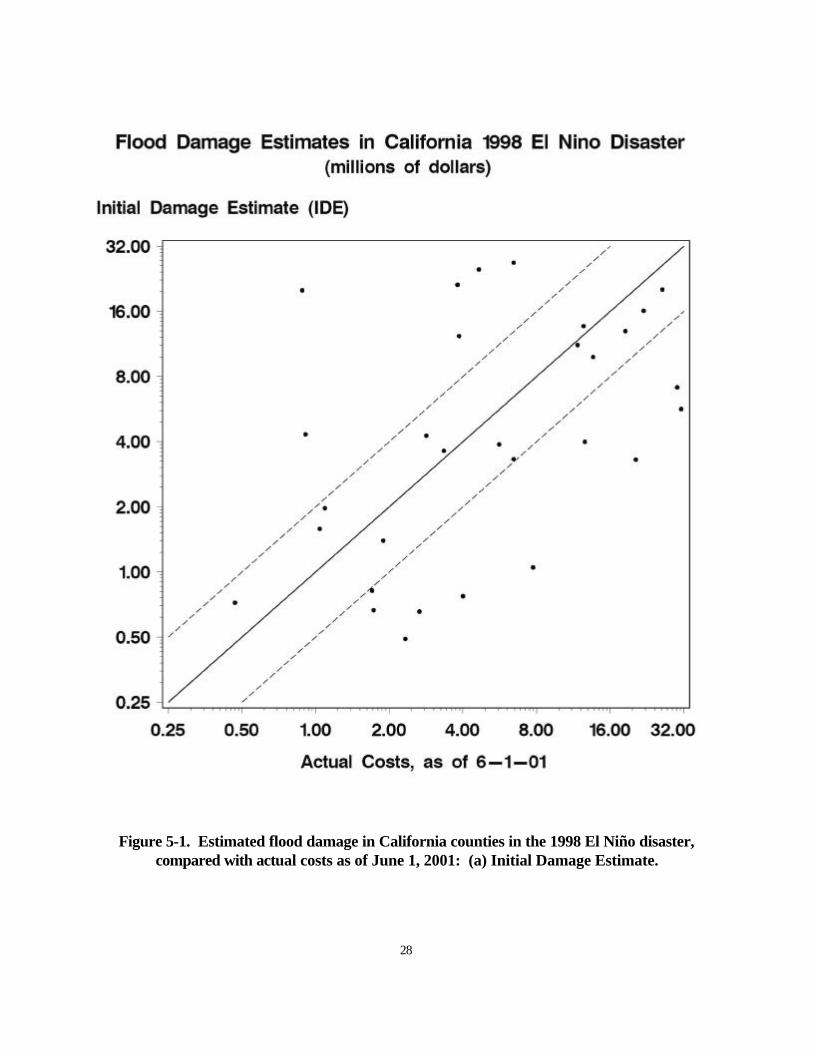
28

Figure 5-1. Estimated flood damage in California counties in the 1998 El Niño disaster, compared with actual costs as of June 1, 2001: (a) Initial Damage Estimate.

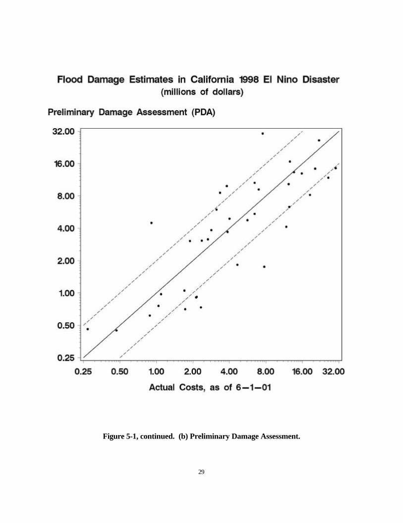
29

Figure 5-1, continued. (b) Preliminary Damage Assessment.

30

were in error by more than a factor of 1.5; and half of the IDEs were in error by more than a factor of 2 (with many off by more than a factor of 4).

Given the methods used by NWS field offices to obtain flood damage estimates (described in Section 2), it is unlikely that the NWS estimates are much better than the IDEs examined here. Thus, when an annual flood damage estimate for a state is less than about $30 million, one should not expect the NWS estimate to depict actual losses accurately. However, the above analysis does not indicate systematic bias in the individual estimates, and errors tend to average out when the estimates are summed.

From the above results, we conclude that aggregation of many damage estimates in floods that have caused high levels of damage ($300 million or more in 1998 dollars) provides reasonably good estimates of total damage. However, estimates at a low level of aggregation ($30 million or less) often are in error by factors of 2 or more. Such small estimates should be used with great caution: Direct comparisons of individual estimates are likely to be misleading. B. Comparison of Damage Estimates from NWS and States

Appropriate data are not available for comparing NWS estimates with actual flood damage costs. However, comparable estimates are available from independent state sources to do an assessment of typical estimation variability.

Every state in the U.S. has an emergency management agency. In July 2000, we wrote to the head of the emergency management agency in each state asking for historical data on flood damage in their state. The letter was followed by a phone call to the appropriate administrator if a response was not received within three weeks. Twenty-one states responded2, but many of them could provide damage information only after 1990 and only related to losses covered by FEMA. Five states either had published historical summaries of flood damage or were able to compile flood damage estimates from their files covering at least 20 years which were based on criteria similar to those used by the NWS.

(1) California: A report (Montane 1999) describes disasters from 1950 through 1998 including for each disaster a brief description, general location, estimated damage, number of deaths, and whether a presidential disaster declaration was issued. We selected the disasters that involved flood, heavy rainfall, or severe storms for this comparison.

(2) Colorado: The state has formally collected flood data since 1937. A report (McLaughlin Water Engineers, Ltd. 1998) summarizes flood history and provides damage estimates for major floods since 1864.

(3) Michigan: A report (Michigan Dept. of State Police 1999) summarizes the 14 floods during 1975–1998 that resulted in a disaster declaration by either the governor or the president. Damage estimates are given for all of the floods that received a presidential declaration and four that received only a gubernatorial declaration.

(4) Virginia: Damage estimates in presidentially-declared flood disasters during 1977–1999 were provided by Michael Cline, State Coordinator of the Virginia Dept. of Emergency

2States that responded were AL, CA, CO, FL, GA, HI, IL, IN, LA, MA, MI, MN, MO, OH, OR, SC, TX, VA, WA, WV, WY.

31

Services (personal communication 2000). (5) Wisconsin: One report on the 1993 Midwest flood summarizes flood losses in Wisconsin

from 1973 through 1992 (FEMA 1993), and another report provides loss estimates for the 1993 flood (Wisconsin Dept. of Natural Resources 1993).

In the state reports, the loss estimates are provided for each major flood event, sometimes

with two or more events occurring in a given year. To match the annual loss estimates provided by NWS-HIC, we added up the flood losses in each state for each year, using calendar years during 1955–1982 and fiscal years (Oct–Sep) during 1983–1998 to match the time periods used in the NWS estimates.3 Our comparison covers a total of 155 years in the 5 states: 44 years each in California and Colorado (1955–1998), 24 years in Michigan (1975–1998), 22 years in Virginia (1977–1998), and 21 years in Wisconsin (1973–1993).

Of course, the state estimates are subject to the same types of error as the NWS estimates – neither is assumed a priori to be more accurate. The intent of this section is to investigate large discrepancies between estimates from different sources in order to understand how estimates of the same event vary and to determine whether some floods are overlooked. In the following analysis, all loss estimates are reported in inflation-adjusted 1995 dollars. When estimates are very low or missing

Table 5-2 provides a comparison of the estimates in all 155 years, with cases along the diagonal (from upper-left to lower-right) showing the closest agreement. An obvious difference between the NWS and state estimates is in the amount of missing data – a result of different purposes of the data. NWS flood loss estimates are collected every year, with relatively small losses included; hence, estimates are missing or zero in only 28 years and are below $5 million in 56 years. In contrast, the state reports focus on more serious floods, so years of relatively low flood loss are not included. The states did not report losses in 91 cases, and included losses below $5 million in only 6 cases.4 The threshold for reporting appears to be somewhat higher in California, where the lowest reported loss was $15 million.

We conclude that these five states do not attach great importance to floods that cause less

than $5 million in damage; therefore, annual losses below that threshold will be described as “low” flood losses. Lumping the low and missing categories together, the NWS and states agree that 78 (50%) of the 155 cases involved little or no flood damage. Disagreements arise, however, when at least one estimate is above $5 million.

3Estimates for 1980-82 were included at this stage of the analysis. California flood damage in Dec 1982 could be attributed differently by the two sources because of the overlap in definition of calendar year 1982 and fiscal year 1983. The other four states did not report losses in Oct-Dec 1982.

4During 1955-98, California reported losses in 26 years (59%), while Colorado reported losses in only 13 years (30%). The other three states reported losses in 33-41% of the years covered by their reports (8 years in Michigan, 9 years in Virginia, and 8 years in Wisconsin).

32

Table 5-2. Crosstabulation of flood damage estimates from the NWS and five states. Estimates are in millions of 1995 dollars.

NWS Estimate

State Estimate

Missing

Est < 5 (Low)

5 < Est < 50 (Moderate)

50 < Est < 500

(High)

500 < Est (Major)

Total

Missing

26

48

14

2

1

91

(59%) Est < 5 (Low)

0

4

2

0

0

6

(4%) 5 < Est < 50 (Moderate)

2

4

13

3

0

22

(14%) 50 < Est < 500 (High)

0

0

5

16

1

22

(14%) 500 < Est (Major)

0

0

0

1

13

14

(9%) Total

28

(18%)

56

(36%)

34

(22%)

22

(14%)

15

(10%)

155

33

Disagreement #1: State estimate above $5 million, NWS estimate missing or low. California describes flood losses of $50 million in 1979 and $15 million in 1984, both years in which the NWS provides no loss estimate. In addition, states claim moderate losses in four years when the NWS estimate is low (< $5 million): Colorado 1969 and 1983 ($20 and $24 million, respectively), California 1972 ($29 million), and Virginia 1998 ($13 million). Because these floods were cited as significant in the state reports, it seems likely that the damage was considerably greater than the NWS estimates would indicate. The differences between estimates range from a factor of 6 in the 1998 Virginia case to a factor of 169 in the 1983 Colorado case.

Out of 84 cases in which the NWS indicated flood losses were low or missing, 78 (93%) were in reasonable agreement with the state reports; but 6 cases in which over $5 million damage was claimed by a state were either overlooked entirely by the NWS or underestimated by a large factor.

Disagreement #2: NWS estimate above $5 million, state estimate missing or low. The top row of Table 5-2 shows 17 cases, not mentioned in the state reports, in which the NWS indicates flood losses over $5 million. In all but one case, the NWS estimate is below $51 million. We assume that some flood damage probably occurred, but the state did not include it in their report. Four of these cases are in Virginia and would have been omitted because they did not receive a Presidential disaster declaration. Excluding Virginia, the three largest NWS estimates are for California, where flood losses are generally high and a $50 million loss might be considered relatively unremarkable.

In one case, however, the NWS estimate is very high: $806 million in Michigan in 1981. This is contradicted by Michigan’s report (Michigan Dept. of State Police 1999), which lists eight floods since 1975 and describes the 1986 flood (with losses of about $400 million) as the most damaging, but makes no mention of a flood in 1981. This blatant error casts doubt on the NWS estimates for 1980–1982, which were derived from broad damage categories in Storm Data, apparently with little or no verification. (See also Section 3 on 1980–1982 damage estimates.) Comparisons of estimates For California, Figures 5-2(a,b) show cases in which at least one estimate is greater than $50 million. For the other states, Figures 5-2(c–f) show cases in which at least one estimate is greater than $5 million. Visually, the graphs are dominated by the major floods (over $500 million), where most of the disagreements appear to be relatively small (except for the erroneous estimate we have already noted for Michigan in 1981). At the moderate-to-high damage levels ($5–500 million), however, some differences are proportionately large. For example, estimates differ by more than a factor of two in California in 1965, 1973, 1976 and 1993, Colorado in 1984 and 1995, Michigan in 1982 and 1998, Virginia in 1979, 1984, 1992 and 1996, and Wisconsin in 1973, 1978, 1980 and 1986.

34

Figure 5-2. Comparison of National Weather Service flood damage estimates with estimates obtained from five states: (a) California, 1955–1977.

35

Figure 5-2, continued. (b) California, 1978–1998.

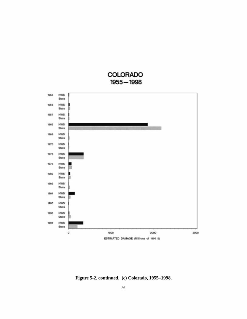
36

Figure 5-2, continued. (c) Colorado, 1955–1998.

37

Figure 5-2, continued. (d) Michigan, 1975–1998.

38

Figure 5-2, continued. (e) Virginia, 1977–1998.

39

Figure 5-2, continued. (f) Wisconsin, 1973–1993.

40

Figure 5-3 is a scatterplot of all cases that have estimates from both NWS and the state. Logarithmic scales are used on the axes to highlight proportional differences in the estimates. The solid diagonal line represents perfect agreement between the estimates. Data points outside of the two dashed lines are cases in which the estimates differ by more than a factor of two. Seventeen cases are above the upper dashed line, representing state estimates more than twice as large as the NWS estimate. Six cases are below the lower dashed line, with NWS estimates more than twice as large as the state estimate.

The closest agreement between state and NWS estimates occurred in floods involving major damage (over $500 million). At the other extreme, the largest proportional disagreements (cases farthest outside the dashed lines) occurred when both sources indicated that flood damage was low or moderate (under $50 million).

From the standpoint of the NWS estimates, when the NWS damage estimate was: (1) moderate ($5–50 million), then 55% of state estimates differed by a factor of 2 or more; (2) high ($50–500 million), then 30% of state estimates differed by a factor of 2 or more; (3) major (over $500 million), then none of the differences exceeded a factor of 1.4.

There are many plausible explanations why agreement might improve as total damage increases. First, the crisis of a major flood spurs studies by numerous agencies. Collection of damage information is more likely to be systematic and complete in a major flood than in a smaller one. Second, agencies are more likely to share information about major floods (which would lead to increased agreement, but does not guarantee greater accuracy). In smaller floods, on the other hand, collection of damage information is likely to be haphazard and there is less interest in checking and correcting early damage estimates. Third, the damage in large floods is aggregated from many individual damage estimates so that random errors tend to cancel out. Small floods involve less aggregation and, hence, relatively larger errors. C. Accuracy: Summary and Conclusions

The following conclusions are drawn from the analysis of accuracy and consistency presented in Sections 4 and 5.

1. The collection and processing of flood damage data by the NWS has been reasonably consistent from 1934 to the present, except during the period 1976–1982. Errors are probably somewhat larger in the first few years after data collection resumed in 1983.

Data from NWS files and other sources made it possible to reconstruct state and national

flood damage estimates for 1976–1979. However, little data was collected during 1980–1982 and large errors were discovered in estimates developed later for that period. As a result, the years 1980–1982 have been excluded from the reanalyzed data sets. Annual compilation of damage estimates resumed in 1983, but depended mainly on information from Storm Data in the first few years. Particularly in 1983–1984, omissions are more likely and estimates probably contain somewhat larger errors because of the use of damage categories.

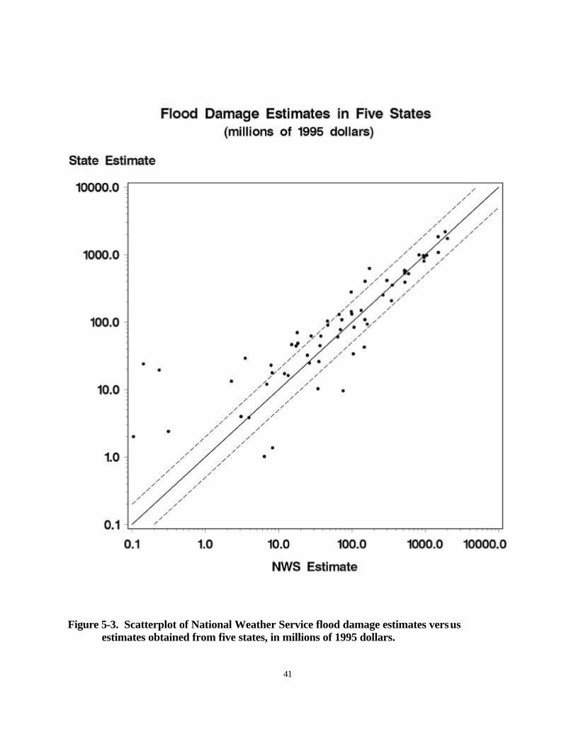
41

Figure 5-3. Scatterplot of National Weather Service flood damage estimates versus

estimates obtained from five states, in millions of 1995 dollars.

42

2. Individual damage estimates for small floods or for local jurisdictions within a larger flood area tend to be extremely inaccurate.

It is rare to have actual cost data to compare with damage estimates. The above analysis of one large flood disaster indicates that, in cases where actual costs are less than $30 million, a large proportion of estimates are off by at least a factor of two and sometimes much more. When damage in a state is estimated to be less than $50 million, estimates from NWS and other sources frequently disagree by more than a factor of two.

3. Damage estimates become more accurate at higher levels of aggregation. Thus NWS estimates totaled over large geographic areas or many years are likely to be fairly reliable (within about a 50% margin of error).

Errors tend to average out, as long as the local estimates are not systematically biased. For example, the sum of estimates from many counties in a large flood area are found to be quite close to the actual total costs for the area as a whole. When damage in a state is estimated to be greater than $500 million, disagreement between estimates from NWS and other sources are relatively small (40% or less). The relatively close agreement between NWS and state estimates in years with major damage is reassuring, since the most costly floods are of greatest concern and make up a large proportion of total flood damage.

4. Floods causing moderate damage are occasionally omitted, or their damage greatly underestimated, in the NWS data sets.

When discrepancies between NWS and state estimates are large, most often the state estimate is the higher one. Occasionally, NWS estimates are missing for floods in which the state claims as much as $50 million damage. Such omissions would have little effect on national total damage estimates. However, they might be important in analyses of damaging floods at the state or river basin level. Researchers studying flood damage in states or river basins should be aware that the NWS estimates occasionally overlook some locally significant damage.

43

6. DEALING WITH DATA OMISSIONS AND INCONSISTENCIES Used appropriately, reanalyzed NWS damage estimates can provide valuable information about historical flood damage in the U.S. But users should be aware of the deficiencies in the damage data sets and choose methods of analysis that guard against misleading results. Omissions and inconsistencies are of particular concern if they introduce systematic biases in the damage estimates that might distort comparisons of flood damage between different time periods or locations. This chapter examines frequency distributions of state damage estimates to evaluate the impact of omissions and inconsistencies and to suggest appropriate methods of analysis. A. Frequency of Damaging Floods at the State Level Few states report flood damage every year; indeed, many states experience damaging floods rather infrequently. In studying the flood damage history of a state or region, it is of interest to know how often damaging floods occur. However, the lack of a damage estimate does not necessarily imply zero flood damage because reporting of dollar damages, particularly in small flood events, is somewhat unreliable. To assure consistent comparisons across different times and locations, it would be helpful to know what levels of damage have been reported fairly consistently. The NWS defines its flood damage data as “loss estimates for significant flooding events” (NWS-HIC 2001). Floods that cause deaths or extensive damage have always received the most attention, but the records do not indicate any formal criteria on which floods to include. When small estimates are submitted, NWS-HIC has usually included them in the damage totals. (An exception occurred during 1993–1998, when local damage estimates below $50,000 were not entered in the flood damage database.) However, field office reports often mention damage without providing dollar estimates. When pressed for a definition of which floods are “significant” enough that intensive efforts are made to obtain complete estimates, NWS-HIC Director Frank Richards offered a rough guideline of at least $1 million in losses (personal communication, 6/27/01). This applies to NWS practice since 1990, but earlier guidelines, if used, are unknown. Frequency distributions of state flood damage estimates suggest that floods with total state damage less than $100,000 (in 1995 dollars) have often gone unreported, and those under $1 million also have sometimes been omitted. Figure 6-1 shows the distribution of all state flood damage estimates in recent years (1983–1999) and in an earlier period (1955–1978). Estimates were missing nearly 30% of the time in the earlier period, and only 16% of the time in recent years. This could imply either fewer damaging floods or different reporting standards in the earlier period — perhaps both. Because the early period had a high frequency of flood damage over $1 million, it is unlikely that the incidence of damage less than $1 million was as small as the distribution suggests. It is likely that lower level damages were not consistently reported before 1980.

44

Figure 6-1. Frequency distributions of annual state flood damages (1995 dollars), 1955–

1978 and 1983–1999.

45

For determining the frequency of damaging floods, we recommend establishing a threshold above which damage estimates are expected to be provided consistently. In our analysis we have chosen to use the frequency of inflation-adjusted state flood damage estimates above $1 million. B. Magnitude of Damages Individual states differ greatly, both in flood frequency and in the magnitude of damage in a “typical” flood event. Figure 6-2 shows, for each state, the estimated total damage during the years 1955–1978 and 1983–1999, as well as the damage in the worst flood year. A few states have had many major floods (e.g. California, Texas). Many others have suffered most of their total damage in just one or two major flood events (including Pennsylvania and Iowa, among the worst in total damage). Many states had no yearly damage greater than $500 million in this period, and there are 10 states whose total damage for the entire 41-year period is less than $500 million. These state comparisons do not include 1979 damage estimates because some estimates for that year are available only for large regions, not for individual states (see Section 3). Estimates of 1979 damage are available for many states, however, and are useful to illustrate how rankings of states by total damage can differ depending on the time period covered. For example, 1979 flood damage in Texas was $3.76 billion — substantially greater than in any of the years included in Figure 6-2. Texas would move from 6th to 3rd place in the rankings if 1979 were included. The frequency distributions of flood damage in each state give another perspective on past flood vulnerability. Table 6-1 shows how states differ in both frequency and severity of damaging floods during 1955–1978 and 1983–1999. The states are ordered by their median annual flood damage based on all 41 years, including years with no reported damage. The number of missing, very low (< $1 million) and relatively high (> $100 million) damage estimates are shown to indicate both frequency and relative magnitudes of flood damage. Three “historical vulnerability categories” can be loosely defined to illustrate the differences between states. (Although the worst flood, indicated by maximum damage, is shown for each state, it is not considered in defining historical categories.) (1) Low vulnerability: Floods are relatively infrequent, and damage is less than about $2 million in the majority of years (1995$). Includes New England states, some mid-Atlantic coastal states, low-population states in the arid west, plus Hawaii and Alaska. Damage rarely exceeds $100 million. (Frequency distributions of flood damage in Maine and New Mexico are surprisingly similar, despite their geographic differences.) (2) Medium vulnerability: Damaging floods occur in most years, and median damage is in approximately the $2 – 8 million range (1995$). Includes most states in the southeast, the lower Mississippi basin, and the Pacific northwest. Most of these states have few instances of flood damage over $100 million. (Louisiana is a notable exception.) (3) High vulnerability: Damaging floods occur in most years, and damage exceeds about $8 million in the majority of years (1995$). Includes states in the upper Mississippi, Missouri,

46

Figure 6-2. States ranked by estimated total damage during 1955–1978 and 1983–1999.

47

Table 6-1. Comparison of Damage Estimates by State, 1955–1978 and 1983–1999. States are ordered by increasing median damage. Missing estimates are treated as zero; all estimates are in millions of 1995 dollars.

State Region

Median Damage

(all years) Maximum Damage*

Years with no estimate

Years with 0<est#1.0

Years with est > 100.

Rhode Island New England 0.00 143. 33 5 1

Delaware 0.00 7. 32 7 0

Massachusetts New England 0.00 774. 25 5 2

New Hampshire New England 0.00 56. 23 6 0

Hawaii 0.00 44. 23 2 0

Connecticut New England 0.00 1881. 21 6 2

Vermont New England 0.00 194 20 9 1

Wyoming Arid West 0.05 53. 17 14 0

Maine New England 0.06 77. 20 3 0

New Jersey 0.06 749. 18 5 8

Alaska (29 yr) 0.07 383. 14 4 1

Maryland &DC 0.14 681. 15 14 1

Nevada Arid West 0.16 616. 13 12 1

Michigan 0.21 528. 17 11 3

N. Dakota N. Central 0.41 3280. 14 9 4

S. Dakota N. Central 0.51 796. 10 13 4

Colorado Arid West 0.57 1866. 11 10 4

S. Carolina 0.66 40. 5 18 0

New Mexico Arid West 0.73 34. 16 6 0

Utah Arid West 0.84 712. 7 14 2

Montana Arid West 1.04 229. 10 10 1

Idaho 1.21 1507. 9 10 2

Wisconsin 1.61 943. 11 8 4

Georgia Southeast 1.86 307. 5 7 3

Virginia 1.91 1042. 9 9 6

Arizona Arid West 2.27 306. 7 9 4

Minnesota 2.40 1006. 4 12 7

48

Florida Southeast 2.48 410. 6 9 5

N. Carolina 3.99 2919. 5 5 3

Oregon Pacific NW 4.06 3143. 2 6 4

Washington Pacific NW 4.32 363. 5 7 3

Louisiana Lower Miss. 5.60 3097. 7 7 10

Tennessee Southeast 6.01 193. 2 8 1

Alabama Southeast 6.10 351. 4 4 3

Arkansas Lower Miss. 6.87 712. 2 6 4

Mississippi Lower Miss. 8.07 1157. 1 3 4

W. Virginia Ohio R. 8.60 782. 1 7 5

Kansas Central 8.61 575. 3 4 6

Oklahoma Central 8.97 1045. 4 8 5

Pennsylvania 10.39 8590. 3 7 6

Nebraska Upper Miss. 13.89 307. 4 4 4

New York 14.60 2305. 7 3 6

Illinois Upper Miss. 15.31 2754. 1 3 8

Iowa Upper Miss. 17.18 5987. 4 6 9

Kentucky Ohio R. 17.67 453. 1 7 7

Indiana Ohio R. 19.29 310. 0 3 3

Ohio Ohio R. 22.06 313. 3 5 4

Missouri Upper Miss. 25.42 3577. 0 7 12

California 45.64 2007. 3 4 13

Texas 77.44 691. 1 1 16

____________________ * Estimates of maximum damage can be misleading. For example, in Idaho the maximum was caused by failure of the Teton Dam in 1976; the worst damage directly from precipitation and streamflow is estimated at $120 million. In Texas, the maximum appears small but much greater damage occurred in a year not covered by this table ($3.76 billion in 1979).

49

and Ohio basins, parts of the mid-Atlantic region, California and Texas. Flood damage over $100 million occurs relatively frequently, especially in Missouri, California, and Texas. Perception of flood damage in a state is influenced by historical experience. A state’s median damage can be taken as the expectation of the flood damage threat in a “typical” year, its maximum damage as the public view of a “major flood”. These categories are useful in describing how state perspectives on flood damage might differ. Although some states in each category have experienced massive flood damage (over, say, $1 billion), such damage occurs most frequently in the high vulnerability category. One might expect that reporting of flood damage by NWS field offices would be influenced by the flood history of an area. In low vulnerability states, floods causing over $1 million damage are notable events and seem unlikely to go unreported. Conversely, in high vulnerability states, damage of $5 million or more occurs frequently so smaller damages might seem unremarkable and be easily ignored. However, the analysis in Section 5 indicates that these expectations are false. In California, a high vulnerability state, the NWS often reports damage under $5 million, but no NWS estimates were provided in two years when the state claimed substantial damage (1979 and 1984).5 Likewise in Colorado, a low vulnerability state, damage of $24 million went virtually unreported in 1983 (the NWS estimate is $140,000). From these examples and others in Section 5, we conclude that omissions of estimates in the $5 – 25 million range in the NWS data sets are not systematically related to the size of a state or its typical damage level; rather, the omissions can be considered random inconsistencies in data collection operations. C. Implications for Analysis of State Damages States typical of the three vulnerability categories are shown in Figures 6-3(a–c) and Table 6-2. California represents the high vulnerability states, Alabama the medium vulnerability states, and Maine the low vulnerability states. In all three states, damage totals for the full 41 year period (Table 6-2) would be affected little by occasional omission of damage under $1 million. Indeed, California and Alabama totals would be affected little by a few $25 million omissions. But in Maine, a $25 million flood is relatively large, representing over 10% of total damage. Its omission could greatly influence the result of, say, a comparison of damages during two time periods. Furthermore, since floods in Maine involve relatively low damage there is less aggregation of damage estimates, therefore less tendency for errors to average out. For low vulnerability regions, we recommend spatial aggregation to reduce the impact of errors and omissions. Several contiguous regional groupings of states with similar frequency distributions are suggested in the second column of Table 6-1. For example, estimates of damage in New England are expected to be more reliable than estimates of damage in Maine. Other groupings might be appropriate depending on the purpose of a particular analysis. 5 The largest known omission — of $50 million damage in California in 1979 — occurred when NWS data collection had been seriously curtailed. It has been corrected in the revised data sets that we provide.

Table 6-2. Levels of annual state flood damage in three states, during all years, 1955–1978 and 1983–1999.

Flood Damage Estimates (Millions of 1995 dollars)

California (High Vulnerability)

Alabama (Medium Vulnerability)

Maine (Low Vulnerability)

Annual State Flood Damage Level N Sum of Damages N Sum of Damages N Sum of Damages

Over $1 billion 3 5,008.4 (47.4%) 0 — 0 —

$100 – 1,000 million 10 4,873.8 (46.1%) 3 601.86 (59.6%) 0 —

$10 – 100 million 14 657.9 (6.2%) 13 332.89 (33.0%) 5 167.66 (72.3%)

$1 – 10 million 7 22.4 (0.2%) 17 72.81 (7.2%) 13 63.25 (27.3%)

$0.1 – 1 million 2 1.1 (0.0%) 4 1.82 (0.2%) 2 0.81 (0.3%)

$0.1 million or less 2 0.1 (0.0%) 0 — 1 0.06 (0.0%)

Missing 3 — 4 — 20 —

Totals 41 10,563.7 (100.0%) 41 1,009.38 (100.0%) 41 231.78 (100.0%)

51

Figure 6-3. Historical flood damage in states representing different levels of vulnerability:

(a) High vulnerability, California.

52

Figure 6-3, continued. (b) Medium vulnerability, Alabama.

53

Figure 6-3, continued. (c) Low vulnerability, Maine.

54

D. Recommendations In summary, the following two procedures are recommended to reduce the impact of errors and omissions in the NWS state damage estimates: 1. To determine the frequency of damaging floods in a state, establish a threshold above which damage estimates are consistently provided and report the number of floods that have exceeded the threshold. Our analysis indicates that reporting of state flood damages greater than $1 million (in 1995 dollars) has been reasonably consistent since 1955, although state damages in the $1 – 50 million range prior to 1990 occasionally went unreported. 2. To reduce the impact of errors and omissions in the estimates, increase the level of aggregation; this can be done either by (a) using total damages in a state or states over an extended period of years, or (b) computing damages for multi-state regions rather than using individual states. This is especially important for statistical analysis of low vulnerability states.

55

7. USE AND INTERPRETATION OF NWS FLOOD DAMAGE DATA “Estimate” is the key word for describing the NWS flood damage data. They do not represent an accurate accounting of actual costs, nor do they include all of the losses that might be attributable to flooding. Rather, they are rough estimates of direct physical damage to property, crops, and public infrastructure. Damage estimates for individual flood events are often quite inaccurate, but as estimates from many events are added together the errors become proportionately smaller. These findings suggest that, at the national level, annual damage totals are reasonably accurate because they are sums of damage estimates from many flood events. Flood damage occurs every year, and the frequency distribution of national damages during 1934–1999 approximates a log normal distribution. Therefore, the national data can be analyzed using conventional parametric statistics. State annual damage estimates are more problematic. Both frequency and magnitude of damage must be considered, because damaging floods do not occur every year in most states. Flood frequency cannot be determined simply by the presence or absence of a damage estimate because reporting, particularly for small floods, is unreliable. (To estimate flood frequency, we recommend establishing a threshold below which estimates are simply classified as “low” or “minimal”, as in Section 6.) Estimates of the magnitude of annual damage are often highly unreliable. In many states, most of the annual damage estimates are below $500 million (in inflation-adjusted 1995 dollars), therefore likely to contain proportionately large errors, as shown in Section 5. Even when damage is greater than $500 million, estimates from different sources have been found to disagree by as much as 40%. Aggregation is one key to reducing estimation errors. To compare flood damages between states or river basins, it is advisable to aggregate the damage estimates over many years and compare the sums. To compare damage between years, it is advisable to aggregate yearly state damage estimates over multi-state regions, or river basin damages over large river drainage systems. Even when the estimates are highly aggregated, the user still needs to be aware that some of the variability is caused by error, and interpret the results accordingly. A. Analyzing Trends Over Time There are several ways of looking at trends in flood damage. Economic damage results from an interaction between flood waters and human activities in the flooded area, so one must consider changes in population and development. Figure 7-1 shows (a) U.S. total flood damage, (b) flood damage per capita, and (c) flood damage per million dollars of tangible wealth.6 (All

6Flood damage per capita is computed by dividing the inflation-adjusted losses for each year by the estimated population on July 1 of that year (www.census.gov). Flood damage per million dollars of tangible wealth uses the net stock of fixed reproducible tangible wealth as estimated by the U.S. Dept. Of Commerce, Bureau of Economic Analysis (www.bea.doc.gov) for December 31 of each year (depreciating stock carried over from prior years). Thus, the flood damage per million dollars of tangible wealth reflects the proportion of the nation’s wealth in that year lost due to floods. All three damage time series have log normal frequency distributions, therefore the displayed trends are transformations of linear trends computed on the logarithm of the damage values.

56

Figure 7-1. Estimated annual flood damage in the United States, 1934–1999: (a) Total flood damage.

57

Figure 7-1, continued. (b) Flood damage per capita.

58

Figure 7-1, continued. (c) Flood damage per million dollars of tangible wealth.

59

estimates are adjusted for inflation.) The three graphs give quite different pictures of how U.S. flood damage has changed over time. Total damage and per capita damage show statistically significant increasing trends since 1934. On the other hand, damage per unit wealth has declined slightly, although the trend is not statistically significant (a = 0.05). Caution #1: In analyzing flood damage over time, it is important to control for changes in population, wealth, or development. B. Comparing States Comparing states on the basis of their historical flood damage is complicated by the rarity of extreme damage. In a limited time period of study, some states will have experienced a low-probability flood event and others will not. Damage totals for the period depend greatly on a few extreme events. Although aggregating state damage estimates over many years helps reduce estimation errors, it does not account for differences in the timing of severe damage. For example, the inclusion of data for just one more year, 1979, would change the position of Texas in the ranking of total damages in Figure 6-2, moving it from 6th to 3rd place (Section 6). Figures 7-2(a, b) compare rankings of the states based on their total flood damage in two periods, 1955–1978 and 1983–1999. Pennsylvania suffered the greatest damage in the earlier period, but its rank slips to 26th in the later period. Iowa moves in the opposite direction, from 28th in the earlier period to first in the later period. In both states, a single flood event determines the first-ranked status. A single year constitutes the majority of damage in many other states, as well. Differences in the timing and location of extreme weather events contribute to quite different rankings during the two periods. Population differences are also an important factor when comparing states. In Figure 7-3, states are ranked according to their annual average damage per capita during 1983–1999, giving a quite different picture than the ranking by total damage in Figure 7-2(b). North Dakota moves to the top, with a whopping $363 damage per person per year (mostly attributable to flooding in 1997), while California slips to 25th place. Caution #2: When comparing damage in different geographical areas, it is important to control for differences in population and in the incidence of extreme weather events during the period of study. C. Comparing Individual Flood Events In comparing annual state estimates, we recommend coarse comparisons using broad damage categories, perhaps similar to those used in Section 5 (low, medium, high, major).7 Uncertainty in the dollar estimates can make comparisons difficult, even in major floods where estimates are highly aggregated. Some of the difficulties are illustrated by the following comparison of two years of major flood damage (over $500 million) in Minnesota in the 1990s.

7For comparing floods at the county level, where damage estimates are extremely unreliable, damage categories can be based on descriptive information instead of dollar estimates. This approach was used in a study of flooding in two Iowa counties (Pielke et al. 2000).

60

Figure 7-2. States ranked based on total flood damage (a) during 1955–1978.

61

Figure 7-2, continued. (b) during 1983–1999.

62

Figure 7-3. States ranked based on average annual flood damage per capita, 1983–1999.

63

1993: Unusually heavy rainfall from May through August over most of the state produced

widespread flooding that resulted in a presidential disaster declaration for 57 of Minnesota’s 87 counties, and an agricultural disaster declaration for an additional eight counties. The NWS estimated damage of $1.0 billion (in 1995 dollars).

1997: Heavy snow and ice followed by spring rains and rapid snowmelt led to severe flooding in

April and May. Damage was extensive in East Grand Forks and many smaller communities. A presidential disaster declaration was issued covering 58 Minnesota counties. Additional storms and flooding in June and July led to another disaster declaration for 7 metropolitan area counties. The NWS estimated damage of $715 million (in 1995 dollars).

In which year was the damage more severe? The answer to this question depends upon how “severe” is defined. The NWS estimates suggest that damage was substantially greater in 1993. However, a report issued by the Minnesota Department of Public Safety leads to the opposite conclusion. Table 7-1 shows actual costs reported in A Decade of Minnesota Disasters (MDPS 2000). (We have excluded costs that are not associated with direct damage, such as temporary housing, hazard mitigation, and economic injury due to loss of business.) FEMA assistance programs, insurance, and SBA loans all indicate that non-agricultural losses were much higher in 1997 than in 1993. A representative of Minnesota’s Division of Emergency Management reinforced this conclusion, telling us that in 1997 entire Minnesota towns were flooded, while in 1993 the main effects of the great Midwest flood occurred in states farther south (Sherrill Neudahl, personal communication, 10/5/00). Agricultural damage was greater in 1993 than in 1997, however. The value of Minnesota’s final crop output in 1993 was 44% less than the average of the previous three years (USDA 2000). In contrast, final crop output in 1997 was equal to the average for the previous three years, suggesting that the floods did little to diminish agricultural productivity that year. Twice as much money was awarded in FSA loans to Minnesota farmers in 1993 as in 1997 (Table 7-1). Lumping agricultural and non-agricultural losses into a single damage estimate is problematic. Enormous discrepancies are found in historical estimates of agricultural damage because of different perspectives on and methodologies for the measurement of losses. For example, one official publication estimated that Minnesota’s total damage in the 1993 flood exceeded $1.7 billion (MDPS 1994) — substantially more than the NWS estimate. Of that, $1.5 billion was attributed to crop “losses” based on the amount that crop production fell short of the previous 4-year average. This is a loss in expectation, perhaps, but not a loss of actual investment. This comparison does not lead us to challenge the NWS estimates for these two flood years. Rather, it provides another reason for caution in interpreting and comparing damage estimates. Given the error magnitudes found in Section 5, the difference of 40% in estimates for the two years is not large enough to say with confidence that one year’s economic damage was worse than the other’s, only that there was major damage in both years. Most Minnesotans would

64

Table 7-1. Minnesota flood damage expenditures in major flood years 1993 and 1997 (in millions of 1995

dollars). Source: MDPS 2000. 1993 1997 Disaster costs itemized by Minnesota Dept. of Public Safety Federal, state, and local government direct costs associated with FEMA assistance programs* (excluding temporary housing and hazard mitigation) 129.7 404.3 Insured losses (estimate) 73.0 154.0 Total direct damage costs (non-agricultural) 202.7 558.3 Small Business Administration loans to cover physical damage SBA physical damage loans for homes and businesses 16.0 74.6 U.S. Dept. of Agriculture loans to farmers, year following disaster Emergency loans through the Farm Service Agency 21.2 10.3 __________________ * FEMA-993-DR-MN in 1993; FEMA-1175-DR-MN and FEMA-1158-DR-MN in 1997.

65

probably consider the floods of 1997 to be much more severe than those of 1993, while farmers might hold the opposite view. Caution #3: Because of the large estimation errors found in the NWS data, estimates for individual floods should be used with caution. For some purposes the comparison of individual floods may be better done using nominal or ordinal data categorizations. For specific events, detailed descriptions should be sought to compare the nature and impacts of the damage. D. Possible Inconsistencies With Other Sources The NWS defines flood damage more narrowly than many other agencies. Emergency management agencies generally include both river and coastal flooding whenever water rises to overflow land that is not normally submerged. In contrast, the NWS estimates include only flooding whose primary cause is rainfall, snowmelt, or river flows, excluding flooding caused by wind-driven waves associated with coastal storms or hurricanes. For example, FEMA records show a Presidential disaster declaration of type “flood” for Massachusetts in February 1978, and the USACE reports $520 million flood damage due to storm surge and huge waves (USACE New England Division 1979; converted to 1995 dollars), but that damage is not included in NWS flood damage estimates. The NWS estimates do include floods caused by dam failure, however. In the NWS record, Idaho’s worst flood resulted from the failure in 1976 of the newly-constructed Teton Dam, with damage estimates in the $1 – 2.3 billion range (in 1995 dollars). Idaho’s largest estimated flood damage due to natural causes was much smaller: $120 million in 1997. Caution #4: Different agencies define “flood” and “flood damage” somewhat differently. Check for incompatibilities between data from different sources before seeking to combine sources or aggregate data. E. Uses of the Reanalyzed NWS Damage Estimates With the precautions noted above, we conclude that the reanalyzed NWS flood damage estimates can be a valuable tool to aid researchers and decision makers in understanding the changing character of damaging floods in the United States. Data sets of annual damage at national, state, and river basin levels are available at www.flooddamagedata.org. In climate research, these data can contribute to understanding the relationship between climatic influences and damaging floods. For example, they have been used to examine the relationship of national and regional flood damage with several measures of precipitation, in a study that controlled for changes in population and wealth (Pielke and Downton 2000). For policy makers and emergency managers, the data provide a nationwide overview of flood vulnerability and can be useful in evaluating policies related to management of flood hazards. For example, we have investigated the role of politics in presidential disaster declaration decisions by comparing disaster declarations involving floods with estimated flood damage (Downton and Pielke 2001).

66

F. Recommendations for Future Collection of Flood Damage Estimates A series of natural disasters in the 1990s, accompanied by skyrocketing costs of federal disaster assistance, has prompted calls for development of national databases to record losses from past and current disasters (Mileti 1999, NRC 1999, Heinz Center 2000). The NWS damage estimates are not reliable enough to be a basis for certain decisions regarding flood policy, such as setting specific flood insurance premiums or evaluating the cost-effectiveness of particular hazard mitigation measures. Better damage data are needed to evaluate the effectiveness of mitigation measures designed to reduce flood losses. Substantial improvement of flood damage records in the U.S. would require additional funding and should have a clear purpose based on intended uses of the data. A committee of the National Research Council (NRC) points out that reliable loss data are critical for cost-effective hazard mitigation and planning for future disaster response. The NRC (1999) report recommends measures for developing a comprehensive and consistent database of losses resulting from natural disasters. Recommendations include: (1) One agency of the federal government should be responsible for compiling the loss data, working with states and localities to collect the data. The Bureau of Economic Analysis (BEA) within the Department of Commerce is suggested as the agency best-suited to the task. (2) The data should focus on direct losses (loss in asset value), including losses that are not reimbursed by insurance or disaster aid. (3) A uniform framework should be used in reporting and compiling loss estimates, classified according to who initially bears the loss (government, businesses, individuals, etc.) and the type of loss (property, agricultural products, deaths and injuries, cleanup and response costs, temporary housing, etc.). These loss estimates should be more complete and accurate than the initial estimates made at the time of a disaster and should include events that may not qualify for a presidential disaster declaration. (4) The database need not contain loss information for every event; rather, the objective should be to compile data on disasters that cross some threshold. The definition of a “major” natural disaster for which loss data are to be compiled should be consistent with expectations for how the data will be used. Clearly, the NWS flood damage database does not provide the level of accuracy and detail envisioned in the NRC recommendations, nor is it intended to do so. Nevertheless, the collection of damage information in severe weather events by NWS field offices provides a model, of sorts, for nationwide collection of damage data. It is administered fairly uniformly throughout the nation, collects information on multiple natural hazards, focuses on direct losses including some unreimbursed losses, and is not limited to declared disasters. As the NWS field offices collect storm damage information, they are in a good position to identify weather events that appear to meet whatever minimum criteria might be established for loss data to be compiled.

67

In the absence of additional funding, only minor improvements can be expected in the NWS collection of flood damage estimates. The following modest changes are suggested to improve accuracy, consistency, and usefulness. (1) Clearly define the purposes of the damage estimates and what types of loss are to be included. (2) Provide uniform instructions to staff members responsible for compiling damage estimates at all NWS field offices. Instructions should include how to obtain damage estimates and some training in damage estimation. (3) It would be valuable to provide separate estimates of different types of loss, as was done in Climatic Data National Summary through 1975. At a minimum, distinguish on-farm losses of agricultural products from other property losses. (4) It is reasonable to set a lower limit below which loss estimates need not be reported, such as $50,000 for a single flood at the county level. The NWS-HIC practice of focusing greatest attention on floods with damage greater than $1 million at the state level is also reasonable. These practices would save staff time and have little impact on total damage estimates.

68

REFERENCES Chadwick, W.L.; Casagrande, A.; Coombs, H.A.; Dowd, M.W.; Fucik, E.M.; Higginson, R.K.;

Leps, T.M.; Peck, R.B.; Seed, H.B.; and Jansen, R.B. (1976). Report to U.S. Department of Interior and State of Idaho on Failure of Teton Dam. Washington, DC: U.S. Government Printing Office.

Coyle, K. (1993). River tinkering worsened flooding. USA Today (July 14). Downton, M.W. and Pielke, R.A. Jr. (2001). Discretion without accountability: Politics, flood

damage, and climate. Natural Hazards Review, 2(4), 157–166. Eikenberry, F.W.; Bogner, N.F.; Lacy, F.P, Jr.; Schuster, R.L.; and Willis, H.B. (1980). Failure

of Teton Dam: Final Report. Stock No. 024-033-00136-8, U.S. Department of the Interior. Washington, DC: U.S. Government Printing Office.

FEMA (Federal Emergency Management Agency) (1993). Interagency Hazard Mitigation Team

Report Wisconsin: FEMA_994_DR_WI, State of Wisconsin, Storms and Flood Events during June and early July 1993. Madison, WI: Interagency Hazard Mitigation Team.

FEMA (1998). Federal Emergency Management Agency Public Assistance Program: Program

Description. Oct. 1, 1998, 9 pp. [http://www.fema.gov/r-n-r/pa/padescp.htm, accessed August 29, 2001.]

FIFMTF (Federal Interagency Floodplain Management Task Force) (1992). Floodplain

Management in the United States: An Assessment Report, Volume 2: Full Report. Washington, DC: L.R. Johnston Associates.

Hamburger, T. (1997). Floods renew interest in climate changes: Is global warming causing

more precipitation? Minneapolis Star-Tribune (April 29). H. John Heinz III Center for Science, Economics, and the Environment (Heinz Center) (2000).

The Hidden Costs of Coastal Hazards: Implications for Risk Assessment and Mitigation. Washington, DC: Island Press.

Kerwin, K. and Verrengia, J.B. (1997). Rare storm loosed Fort Collins flood: Hazard experts say

deluge should serve as ‘wake-up call’ for growing population. Rocky Mountain News (August 3).

Labaton, S. (1993). US weighs scrapping levees for flood control. New York Times (August 28). Marrero, Jose (1979). Danger: Flash floods. Weatherwise (February): 34–37. Marrero, Jose (1980). Flash floods: Second costliest year. Weatherwise (February): 21–23. McLaughlin Water Engineers, Ltd. (1998). Statewide River Rehabilitation and Floodplain

69

Management Needs Inventory. Denver, CO: Colorado Water Conservation Board. Michigan Department of State Police (1999). Riverine and Great Lakes flooding. Michigan

Hazard Analysis. Emergency Management Division, Michigan Department of State Police.

Mileti, D.S. (1999). Disasters by Design: A Reassessment of Natural Hazards in the United

States. Washington, D.C.: Joseph Henry Press. Minnesota Department of Public Safety (MDPS) (1994). The Great Flood of 1993: The

Minnesota Experience. St. Paul, MN: Minnesota Department of Public Safety, Division of Emergency Management. 26 pp.

Minnesota Department of Public Safety (MDPS) (2000). A Decade of Minnesota Disasters: A

Historical Look at Minnesota Disasters in the 1990s. St. Paul, MN: Minnesota Department of Public Safety, Division of Emergency Management. 38 pp.

Montane, V. (1999). Governor’s Office of Emergency Services, Origins and Development: A

Chronology, 1917–1999. Rancho Cordova, CA: Governor’s Office of Emergency Services, Rancho Cordova, CA 95741.

NOAA (National Oceanic and Atmospheric Administration) (1959–1999, passim). Storm Data.

Asheville, NC: National Climatic Data Center. NOAA (1976). The Cooperative Observer, Western Region XIV(3): 2. NOAA (1977). Johnston, Pennsylvania Flash Flood of July 19–20, 1977. Natural Disaster

Survey Report 77-1. Rockville, MD. NOAA (1977). Kansas City Flash Flood of September 12–13, 1977. Natural Disaster Survey

Report 77-2. Rockville, MD. NOAA. (2000). Historical Weatherfacts for the U.S. http://www.awc_kc.noaa.gov/wxfact.html

[accessed September 20, 2001]. NRC (National Research Council) (1999). The Impacts of Natural Disasters: A Framework for

Loss Estimation. Washington, DC: National Academy Press. 80 pp. NWS (National Weather Service) (1950–1980, passim). Climatological Data National Summary.

Asheville, NC. (Years 1975, 1977). NWS (1985). Storm data and related reports. Operations Manual Issuance 85-13. Silver Spring,

MD: U.S. Dept. Of Commerce. NWS (1994). Storm data and related reports. Operations Manual Issuance 94-5. Silver Spring,

MD: U.S. Dept. Of Commerce.

70

NWS-HIC (National Weather Service-Hydrologic Information Center) (2001). Flood Losses.

http://www.nws.noaa.gov/oh/hic/flood_stats/Flood_loss_time_series.htm [accessed August 29, 2001].

Patton, A. (1993). From Harm’s Way: Flood-Hazard Mitigation in Tulsa, Oklahoma. Tulsa,

OK: City of Tulsa. Pielke, R.A. Jr. and Downton, M.W. (2000). Precipitation and Damaging Floods: Trends in the

United States, 1932–1997. J. Climate, 13(20), 3625–3637. Pielke, R.A. Jr.; Downton, M.W.; Miller, J.Z.B.; Changnon, S.A.; Kunkel, K.E.; and Andsager,

K. (2000). Understanding Damaging Floods in Iowa: Climate and Societal Interactions in the Skunk and Raccoon River Basins. Palo Alto, CA: Electric Power Research Institute.

Tennessee Valley Authority (TVA) (1978). Flood of April 1977 in the Tennessee River Basin.

Knoxville, TN: TVA. USACE (U.S. Army Corps of Engineers) (1983–2001, passim). Army Corps of Engineers

Annual Damage Report to Congress. Washington, DC: U.S. Government Printing Office. USACE, Albuquerque District (1978). Flood Report: flood of 19 August 1978; White Sands,

New Mexico. Albuquerque, NM: The District. USACE, Albuquerque District (1979a). Flood Report: Flood Report of 24 September 1978,

Presidio, Texas. Albuquerque, NM: The District. USACE, Albuquerque District (1979b). Post Flood Report: Southern Colorado, Northern New

Mexico, snow melt flood, Mar–Jun 1979. Albuquerque, NM: The District. USACE, Buffalo District (1978). Report of Flood, 14–16 March 1978, Chagrin and Grand

Rivers, Ohio. Buffalo, NY: The District. USACE, Los Angeles District (1978). 6–10 October 1977 Flood Damage Report on Storm and

Floods on Santa Cruz, Gila, and San Pedro Rivers, Arizona. Los Angeles, CA: The District.

USACE, Los Angeles District (1979a). Flood Damage Report 28 February–6 March 1978 on

the Storm and Floods in Maricopa County, Arizona. Los Angeles, CA: The District. USACE, Los Angeles District (1979b). Flood Damage Report: Phoenix Metropolitan Area,

December 1978 Flood. Los Angeles, CA: The District. USACE, Los Angeles District (1980). Flood Damage Report: Southcentral Arizona and

Southwestern New Mexico, December 1978 Flood. Los Angeles, CA: The District.

71

USACE, Little Rock District (1978). Post disaster report: Fourche Creek Basin. Little Rock, AR: The District.

USACE, New England Division (1979). A Report on the Assessment of Flood Damages

Resulting from the Storm of 6–7 February 1978 along the Coastline from Orleans, Massachusetts to New Castle, New Hampshire. Waltham, MA: New England Division.

USACE, Portland District (1978). Postflood Report, November–December 1977 Floods in the

Portland District, Oregon and Washington. Portland, OR: The District. USACE, St. Paul District (1979). Red River of the North and Souris River post flood report

1979. St. Paul, MN: The District. U.S. Bureau of Economic Analysis (2001). Price indexes for Gross Domestic Product and Gross

Domestic Purchases. GDP and Other Major NIPA Series. [http://www.bea.doc.gov/bea/dn1.htm, accessed January 17, 2002.]

U.S. Department of Agriculture (1895–96; 1933–34, passim) Report of the Chief of the Weather

Bureau. Washington, DC: U.S. Government Printing Office. U.S. Department of Agriculture (USDA) (2000). Value added to the U.S. economy by the

agricultural sector via the production of goods and services, 1990–1999, Minnesota. [http://usda.mannlib.cornell.edu/, Net Value Added, accessed October 9, 2000.]

USGS (U.S. Geological Survey) (1991). National Water Summary 1988–89–Hydrologic Events

and Floods and Droughts. United States Geological Survey Water Supply Paper 2375. Washington, DC: U.S. Government Printing Office.

USGS and NOAA (1979). Storm and Flood of July 31 – August 1, 1976, in the Big Thompson

River and Cache la Poudre River Basins, Larimer and Weld Counties, Colorado. USGS Professional Paper 1115. Washington, DC: U.S. Government Printing Office.

USGS and NOAA (1984). Floods of May 1978 in Southeastern Montana and Northeastern

Wyoming. USGS Professional Paper 1244. Washington, DC: U.S. Government Printing Office.

U.S. Weather Bureau (1934–1949, passim). Monthly Weather Review. Boston, MA: American

Meteorological Society. Wagner, A.J. (1982). The weather and circulation of 1981. Weatherwise, Feb. 1982, pp. 4–12. Ward, R.C. (1990). Principles of Hydrology. London: McGraw-Hill Publishing Co. Wisconsin Department of Natural Resources (1993). The Floods of 1993: The Wisconsin

Experience. Madison, WI: Bureau of Water Regulation and Zoning, Wisconsin Department of Natural Resources.

72

ABBREVIATIONS DSR – Damage Survey Report FEMA – Federal Emergency Management Agency IDE – Initial Damage Estimate NOAA – National Oceanic and Atmospheric Administration NWS – National Weather Service NWS-HIC – National Weather Service, Hydrologic Information Center OES – California Governor’s Office of Emergency Services PDA – Preliminary Damage Assessment TVA – Tennessee Valley Authority USACE – U.S. Army Corps of Engineers USDA — U.S. Department of Agriculture USGS – U.S. Geological Survey WCM – Warning Coordination Meteorologist

73

Appendix A

COMPILATION OF DAMAGE ESTIMATES FOR 1976–1979 Monthly damage estimates by river basin in 1976 and 1977 were published in Climatological Data National Summary. NWS staff prepared some 1978 and 1979 estimates which were summarized in Weatherwise (Marrero 1979, 1980). We augmented these estimates with unpublished information housed at NWS-HIC, including reports from regional NWS offices, preliminary tabulation sheets, and notes made by NWS employees. Wherever possible, we also compared damage estimates from NWS-HIC files with reports on specific floods by other agencies, including USACE, USGS, and NOAA. Final estimates were chosen using the following rules:

• In order to change any estimates in the NWS tabulated data set, a published source had to provide good reason to doubt the NWS estimates and the published source had to provide more reliable estimates.

• There were instances when we had to choose between two or more estimates. In general, we chose published source estimates over NWS "grey" sources.

• Asterisks were added to the estimates wherever published sources indicated that a damaging flood occurred but provided no estimates.

1976 Flood Damage Estimates Reconstructed 1976 damage estimates by state and month are shown in Table A-1. Data sources are as follows:

• September in California is from the NOAA Cooperative Observer (NOAA 1976). • July in Colorado is from a USGS/NOAA report (1979). • May in Oklahoma is from a report concerning flood hazard mitigation in Oklahoma

(Patton 1993). • All other damage estimates are from NWS notes and summaries archived at NWS-HIC,

which had been compiled for publication in Climatological Data National Summary, but had not been published.

1977 Flood Damage Estimates Reconstructed 1977 damage estimates by state and month are shown in Table A-2. Data sources are as follows:

• The following totals are from USACE reports: October in Arizona (USACE, Los Angeles District 1978) and December in Oregon and Washington (USACE, Portland District 1978).

• The estimate for a flood in Kansas City, Kansas and Kansas City, Missouri in September of 1977 is from NOAA (1977) and USGS (1991) reports.

• 1977 damage totals for Tennessee, Virginia, and West Virginia have been changed based on information on April flooding in Appalachia from a TVA flood report (TVA 1978).

• All other damage estimates are from NWS notes and summaries archived at NWS-HIC. 1978 Flood Damage Estimates Reconstructed 1978 damage estimates by state and month are shown in Table A-3. It was more difficult to piece together the flood estimates for 1978 and 1979 than for 1976 and 1977.

74

Several different sets of state-level estimates exist in the NWS files for 1978, and in many cases the estimates do not agree. Data sources are as follows:

• All estimates for California are from the California Office of Emergency Services (Montane 1999).

• Most of the entries represented by asterisks rather than damage figures are based on information in Storm Data. In these cases it was apparent that flooding had occurred, but damage figures were not available.

• The following numbers are from USACE reports: March in Arizona (USACE, Los Angeles District 1979a); March in Ohio (USACE, Buffalo District 1978); August in New Mexico (USACE, Albuquerque District 1978); September in Arkansas (USACE, Little Rock District 1978); September in Texas (USACE, Albuquerque District 1979a); December in Arizona (USACE, Los Angeles District 1979b and USACE, Los Angeles District 1980); and December in New Mexico (USACE, Los Angeles District 1980).

• Montana and Wyoming in May are from a jointly authored USGS/NOAA paper (USGS 1984).

• The following estimates are from Marrero (1979): March in Nebraska and Indiana; April in North Dakota and Virginia; May in Louisiana and Texas; July in Alabama, Minnesota, and Wisconsin; August in Texas; and September in Louisiana.

• The following estimates are from Storm Data: May in Arkansas; July in Colorado; August in Illinois, Indiana, and Maryland; and December in Idaho.

• All other estimates are from NWS files. 1979 Flood Damage Estimates Reconstructed 1979 damage estimates by state and month are shown in Table A-4. Data sources are listed below. Users of 1979 estimates should note that a flood in “New Jersey, New York, and southern New England” in January caused $62 million in damage (Marrero 1980). This estimate could not be assigned to individual states. Similarly, a flood in April in Louisiana, Mississippi, and Alabama caused $1 billion in damage that could not be assigned to individual states (Marrero 1980). These floods are included in the national total for 1979, but not in the state estimates.

• All estimates for Virginia are from the state emergency management office (Michael Cline, personal communication 2000).

• The following estimates are from Marrero (1980): March in Indiana and Iowa; April in Texas; July in Texas; September in Maryland, Louisiana, and Texas; October in Kansas and Florida; and November in Hawaii.

• The following are from USACE reports: March in Minnesota and North Dakota (USACE, St. Paul District 1979) and June in New Mexico (USACE, Albuquerque District 1979b).

• Estimates from Storm Data include: February in Arkansas; April in Arkansas, Florida, Illinois; March in Florida and New York; May in South Dakota; June in Colorado; July in Alabama, Illinois, New York, and West Virginia; August in Minnesota, Utah, and West Virginia; and September in Florida.

• February in Hawaii is from USGS (1991). • April in Ohio is from NWS notes. • All other estimates are from NWS files.

75

Table A-1. 1976 damage estimates (thousands of current dollars) State Jan. Feb. Mar. Apr. May June July Aug. Sep. Oct. Nov. Dec. Total Alabama 4,610 100 * 4,710 Alaska * 0 Arizona * * 6,000 6,000 Arkansas * 0 California * 120,100 * 120,100 Colorado 35,540 * 35,540 Connecticut 7,100 7,100 Delaware 0 Florida * * * 0 Georgia * 1,450 6,650 30 8,130 Hawaii 270 270 Idaho 650,000 * 650,000 Illinois 1,570 * 1,800 3,370 Indiana 3,130 550 3,680 Iowa 160 160 Kansas 110 1,220 1,330 Kentucky * 0 Louisiana * 0 Maine 860 * 2,500 3,360 Maryland 4,900 4,900 Massachusetts 1,000 * 1,000 Michigan * * 790 * 790 Minnesota 0 Mississippi 2,840 2,840 Missouri 810 * * 810 Montana 50 50 Nebraska 0 Nevada 200 200 New Hampshire 0 New Jersey * 0 New Mexico * 500 * 500 New York * 1,100 2,120 11,000 14,000 9,000 700 100 38,020 North Carolina 200 8,920 * 9,120 North Dakota 2,420 2,420 Ohio 40 40 Oklahoma 34,250 18,390 52,640 Oregon 1,040 130 * 1,170 Pennsylvania * 410 30 * 440 Rhode Island 0 South Carolina * * 840 7,000 3,330 40 11,210 South Dakota * 5,500 5,500 Tennessee 200 200 Texas 2,940 200 30,000 250 33,390 Utah 0 Vermont * * * * * 0 Virginia * 0 Washington 2,500 2,500 West Virginia * 3,260 3,260 Wisconsin * 0 Wyoming 100 * 100 1,040 8,050 2,670 16,990 50,910 705,530 69,350 21,600 127,050 11,590 0 70 1,014,850 * indicates that a flood occurred, but damage figures are unavailable or under $30,000.

76

Table A-2. 1977 damage estimates (thousands of dollars) State Jan. Feb. Mar. Apr. May June July Aug. Sep. Oct. Nov. Dec. Total Alabama 610 3,490 660 4,760 Alaska 200 * * 200 Arizona 340 * 15,250 15,590 Arkansas 130 * 130 California 28,500 28,500 Colorado 750 * * 500 1,250 Connecticut * 1,520 50 * 1,570 Delaware 0 Florida 140 140 Georgia 240 1,350 2,570 4,160 Hawaii 0 Idaho * 0 Illinois * 830 2,880 1,840 1,640 7,190 Indiana 450 750 3,690 3,270 8,160 Iowa * * * * 0 Kansas * 6,350 40,000 46,350 Kentucky 100,000 * * * 1,000 101,000 Louisiana 48,040 * * 48,040 Maine 4,190 4,190 Maryland 0 Massachusetts * 0 Michigan * * 0 Minnesota * 6,000 1,870 7,870 Mississippi * 2,780 2,780 Missouri 2,500 * 50,000 52,500 Montana 0 Nebraska * * * 870 720 1,590 Nevada 0 New Hampshire 610 610 New Jersey 95,880 95,880 New Mexico * * 0 New York 4,540 460 1,840 3,760 * 10,600 North Carolina * 500 52,000 52,500 North Dakota 80 80 Ohio * 370 370 Oklahoma * 12,000 720 12,720 Oregon 10,690 10,690 Pennsylvania * 330,020 * * 330,020 Rhode Island 0 South Carolina * 80 160 20 260 South Dakota * 0 Tennessee 21,000 21,000 Texas 50 2,000 250 * * * 50 100 2,450 Utah * 260 40 300 Vermont 2,710 2,710 Virginia 242,500 1,400 24,800 268,700 Washington 140 * 5,490 5,630 West Virginia * 50,000 * 500 50,500 Wisconsin 0 Wyoming 100 * * 100 Total U.S. 140 50 19,050 471,140 15,930 6,490 331,690 36,850 95,350 26,540 176,770 21,090 1,201,090 * indicates that a flood occurred, but damage figures are unavailable or under $30,000.

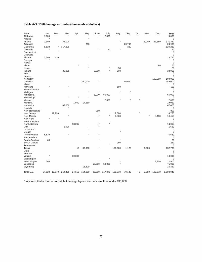
77

Table A-3. 1978 damage estimates (thousands of dollars) State Jan. Feb. Mar. Apr. May June July Aug. Sep. Oct. Nov. Dec. Total Alabama 1,000 * * * 2,000 3,000 Alaska * * 0 Arizona 7,100 33,100 * 8,000 83,160 131,360 Arkansas 200 23,700 23,900 California 6,130 * 117,800 300 124,230 Colorado * * 70 * 70 Connecticut * 0 Delaware 0 Florida 3,300 420 * 3,720 Georgia * 0 Hawaii 0 Idaho * * 60 60 Illinois * * 50 50 Indiana 35,000 3,000 * 960 38,960 Iowa * 0 Kansas 0 Kentucky 100,000 100,000 Louisiana 100,000 * 45,000 145,000 Maine 0 Maryland * * 150 150 Massachusetts 0 Michigan * * * * 0 Minnesota 5,000 60,000 65,000 Mississippi * * * 0 Missouri 2,000 * * * 2,000 Montana 1,500 17,560 19,060 Nebraska 67,000 67,000 Nevada * 0 New Hampshire 900 900 New Jersey 12,220 * 2,500 * 14,720 New Mexico * * * 6,000 * 8,450 14,450 New York * * 0 North Carolina 0 North Dakota 13,000 * * 13,000 Ohio 1,520 * 1,520 Oklahoma * 0 Oregon * 0 Pennsylvania 6,630 * * * 6,630 Rhode Island 0 South Carolina 60 * * 60 South Dakota 250 250 Tennessee * 0 Texas 10 30,000 * 100,000 1,120 1,600 132,730 Utah 0 Vermont 0 Virginia * 10,000 10,000 Washington * 0 West Virginia 700 * * 2,200 2,900 Wisconsin 18,000 53,000 * 71,000 Wyoming 16,320 16,320 Total U.S. 24,920 12,640 254,420 24,510 164,080 26,900 117,070 109,910 70,120 0 9,600 193,870 1,008,040 * indicates that a flood occurred, but damage figures are unavailable or under $30,000.

78

Table A-4. 1979 damage estimates (thousands of dollars) State Jan. Feb. Mar. Apr. May June July Aug. Sep. Oct. Nov. Dec. Total Alabama * # 500 500 Alaska * * * 0 Arizona * 0 Arkansas 620 2,000 * * * 2,620 California 25,900 25,900 Colorado * 50 50 Connecticut # 0 Delaware * 0 Florida 4,990 15,000 1,000 1,000 21,990 Georgia * * * 0 Hawaii 6,000 5,000 11,000 Idaho * * 0 Illinois * 32,000 250 * 32,250 Indiana 15,000 1,000 * 16,000 Iowa 2,000 * * 2,000 Kansas * 7,000 7,000 Kentucky * * 0 Louisiana * # * 8,000 8,000 Maine 0 Maryland * 69,000 69,000 Massachusetts # 0 Michigan * 0 Minnesota 10,140 * * * 3,000 13,140 Mississippi * # * 0 Missouri * * * 0 Montana * 0 Nebraska * * * * 0 Nevada * * 0 New Hampshire * 0 New Jersey # * * 0 New Mexico * 3,210 3,210 New York # * 3,920 * * 14,850 * 18,770 North Carolina * 0 North Dakota 20,100 * 20,100 Ohio 60,000 * 60,000 Oklahoma * * * 0 Oregon * 0 Pennsylvania * * * * * * 0 Rhode Island # 0 South Carolina * 0 South Dakota 49,000 49,000 Tennessee * * * * * 0 Texas * * 500,000 * * 750,000 * 750,000 * 2,000,000 Utah 130 130 Vermont 0 Virginia * * 7,800 * 17,000 24,800 Washington 3,100 * 3,100 West Virginia * 2,000 2,000 Wisconsin * * * 0 Wyoming * 0 LA, MS, AL 1,000,000 1,000,000 NY,NJ,CT,MA,RI 62,000 62,000 Total U.S. 62,000 6,620 56,150 1,609,000 49,000 29,160 776,400 6,230 828,000 25,000 5,000 0 3,452,560 * indicates that a flood occurred, but damage figures are unavailable or under $30,000. # Damage estimate is included in an estimated total for several states.

79

Appendix B

ESTIMATED FLOOD DAMAGE, BY STATE Damage estimates are given in current dollars for the year in which the damage occurred. To adjust for inflation, the estimates can be converted to 1995 dollars by dividing by the implicit price deflator in Column 2 (U.S. Bureau of Economic Analysis 2001). Estimates are for calendar years during 1955–1979, and for fiscal (or water) years during 1983–2000. For example, fiscal/water year 1990 covers from October 1, 1989, through September 30, 1990. An entry of zero indicates that no damage estimate was reported. It can be assumed that actual flood damage was small, but it is quite possible that some damage occurred. Data are unavailable for 1980–1982 and for Alaska before 1967.

80

Damage in Thousands of Current Dollars

Deflator AL AK AZ AR CA CO CT DE 1955 0.20163 3,379 226 61 165,767 2,567 379,360 117 1956 0.20846 720 0 255 8,745 5,135 0 0 1957 0.21539 2,324 0 27,938 13 2,901 0 0 1958 0.22059 872 0 6,202 33,063 240 0 0 1959 0.22304 0 100 3,090 4 0 0 0 1960 0.22620 670 0 580 516 0 750 0 1961 0.22875 12,625 325 3,503 95 0 0 0 1962 0.23180 3,529 1,000 91 2,780 80 0 0 1963 0.23445 1,280 0 2,500 11,834 50 0 0 1964 0.23792 5,343 55 598 229,168 0 0 0 1965 0.24241 723 11,330 143 11,321 452,293 0 0 1966 0.24934 2,366 3,050 5,055 24,347 707 0 0 1967 0.25698 1,695 98,550 3,576 1,497 1,370 0 0 0 1968 0.26809 408 0 188 21,099 0 0 100 0 1969 0.28124 88 0 0 3,411 423,296 66 528 0 1970 0.29623 10,891 0 5,000 639 47,798 2,040 0 0 1971 0.31111 2,170 8,631 3,476 2,549 3,522 0 0 50 1972 0.32436 2,278 1,090 20,868 1,780 1,132 15 15,414 0 1973 0.34251 5,439 1,500 0 129,579 9,480 121,383 1,950 0 1974 0.37329 1,731 0 2,605 8,746 27,124 0 0 5 1975 0.40805 19,815 0 927 21,387 1,845 0 9,360 0 1976 0.43119 4,710 0 6,000 0 120,100 35,540 7,100 0 1977 0.45892 4,760 200 15,590 130 28,500 1,250 1,570 0 1978 0.49164 3,000 0 131,360 23,900 124,230 70 0 0 1979 0.53262 # 0 0 2,620 25,900 50 # 0 1980 0.58145 1981 0.63578 1982 0.67533 1983 0.70214 29,431 0 179,938 500,000 673,000 100 0 0 1984 0.72824 23,000 7,150 223,000 5,000 0 107,050 81,700 5,000 1985 0.75117 1,700 50 1,350 19,823 0 7,000 0 50 1986 0.76769 0 0 3,000 2,240 402,000 166 0 0 1987 0.79083 755 20,000 7 15,045 1,015 0 5,000 0 1988 0.81764 1,721 500 71 12,612 52,353 0 0 0 1989 0.84883 178 6,000 33,636 2,320 38,738 481 800 1,600 1990 0.88186 120,000 0 3,220 143,056 570 130 10 0 1991 0.91397 15,055 0 258 12,006 3,376 2,820 16 0 1992 0.93619 320 7,302 5,189 909 93,152 1,602 10,366 2 1993 0.95872 0 0 228,900 2,680 165,920 100 0 0 1994 0.97870 112,696 74,000 1,616 2,024 1,792 1,242 1,316 741 1995 1.00000 0 10,025 6,618 0 1,495,960 18,240 0 0 1996 1.01937 1,649 0 701 205 13,205 4,058 2,092 300 1997 1.03925 1,354 1,271 85 12,874 2,086,125 358,890 52 0 1998 1.05199 368,938 314 66 2,045 621,588 2,550 40 0 1999 1.06677 4,663 0 12,796 1,777 14,176 50,675 1,112 0 2000 1.09113 3,087 110 90 2,773 9,238 297 6,010 0 # Damage estimate available for large region, but not for individual state.

81

Damage in Thousands of Current Dollars

Deflator FL GA HI ID IL IN IA KS 1955 0.20163 105 1 0 1,371 102 1,003 35 474 1956 0.20846 1,891 212 0 6,222 1,026 4,021 51 33 1957 0.21539 0 1,068 0 20,896 1,206 66,748 1,543 9,164 1958 0.22059 0 323 400 3 17,970 52,302 7,508 4,606 1959 0.22304 150 0 0 500 1,506 12,958 128 4,061 1960 0.22620 12,047 392 0 0 7,503 2,649 7,612 1,947 1961 0.22875 317 5,236 0 939 11,553 13,306 9,389 13,397 1962 0.23180 1,481 0 0 8,112 891 670 6,778 1,826 1963 0.23445 0 445 2,300 2,766 513 8,266 70 168 1964 0.23792 426 3,641 0 11,704 3,044 12,327 240 370 1965 0.24241 144 397 0 4,184 30,564 20 32,462 29,792 1966 0.24934 548 1,628 0 0 577 3,098 904 97 1967 0.25698 95 23 1,029 792 2,629 4,618 4,416 15,093 1968 0.26809 46 133 2,500 0 2,576 22,463 1,650 2,304 1969 0.28124 2,858 79 0 111 9,095 6,672 6,233 10,991 1970 0.29623 145 348 0 38 9,124 2,300 977 4,138 1971 0.31111 476 243 500 1,187 462 1,690 684 1,644 1972 0.32436 41,206 328 0 355 5,927 4,700 13,262 1,646 1973 0.34251 2,282 5,143 0 0 258,704 6,326 12,724 53,772 1974 0.37329 23,050 405 3,869 36,118 75,068 15,805 56,367 3,700 1975 0.40805 15,839 3,002 0 378 20,598 12,317 7,300 3,255 1976 0.43119 0 8,130 270 650,000 3,370 3,680 160 1,330 1977 0.45892 140 4,160 0 0 7,190 8,160 0 46,350 1978 0.49164 3,720 0 0 60 50 38,960 0 0 1979 0.53262 21,990 0 11,000 0 32,250 16,000 2,000 7,000 1980 0.58145 1981 0.63578 1982 0.67533 1983 0.70214 0 0 0 2,200 202,500 20,000 0 0 1984 0.72824 200,000 5,050 6,055 1,000 7,992 22,194 600,550 50,050 1985 0.75117 30,000 0 3,100 0 11,500 50,000 50 5,000 1986 0.76769 7,275 2,000 0 2,005 104,705 2,500 45,307 181,700 1987 0.79083 645 1,470 2,050 17 150,000 1,906 16,755 152,000 1988 0.81764 50,350 230 35,647 0 102 89 0 0 1989 0.84883 2,109 1,792 3,392 178 1,600 716 7,286 3,394 1990 0.88186 500 30,658 665 113 71,045 105,550 351,401 2,048 1991 0.91397 0 106,158 23,715 2,574 19,834 89,504 195,703 16,551 1992 0.93619 41,938 1,156 9,260 224 189 45,424 50,800 10,127 1993 0.95872 2,080 7,340 2,910 0 2,640,140 9,550 5,740,000 551,070 1994 0.97870 182,605 300,000 3,700 0 32,606 2,852 9,124 10,437 1995 1.00000 18,536 8,845 0 2,096 27,240 6,789 3,498 8,874 1996 1.01937 158,001 2,581 1,935 49,400 107,585 21,575 165,265 3,969 1997 1.03925 49,707 464 0 125,060 4,295 68,598 3,680 102 1998 1.05199 431,311 166,291 0 1,005 2,380 19,611 168,101 4,888 1999 1.06677 60,080 8,520 0 1,297 3,666 50,124 111,221 60,030 2000 1.09113 499,080 2,101 400 85 3,113 819 14,877 250 # Damage estimate available for large region, but not for individual state.

82

Damage in Thousands of Current Dollars

Deflator KY LA ME MD MA MI MN MS 1955 0.20163 6,629 30 0 5,450 155,982 0 0 3,132 1956 0.20846 568 0 0 888 0 1,278 11 1,270 1957 0.21539 55,233 4,147 0 0 0 0 9,128 2,693 1958 0.22059 3,817 2,842 0 100 0 0 17 13,826 1959 0.22304 2,480 0 61 0 0 0 50 280 1960 0.22620 3 112 0 0 6,400 1,181 212 744 1961 0.22875 12,969 6,074 800 0 0 0 552 15,918 1962 0.23180 16,885 1,908 0 0 0 0 1,290 1,982 1963 0.23445 36,917 0 0 0 0 0 26 19 1964 0.23792 35,476 30 0 0 0 0 0 3,152 1965 0.24241 1,044 0 0 53 0 0 97,603 1,931 1966 0.24934 1,671 250 528 0 0 0 4,300 2,706 1967 0.25698 17,583 0 0 125 0 0 0 1,192 1968 0.26809 6,036 2,810 0 0 35,000 100 1,197 6,269 1969 0.28124 8,075 251 300 200 0 13 67,168 1,900 1970 0.29623 707 1,000 0 15 0 0 4,350 3,586 1971 0.31111 6,099 0 0 8,600 0 0 15 12,431 1972 0.32436 15,841 100 0 220,739 10 10 64,318 10,248 1973 0.34251 10,491 334,904 11,200 0 0 530 242 226,885 1974 0.37329 5,218 10,343 3,000 0 0 240 16,939 27,827 1975 0.40805 26,302 90,204 0 27,200 0 54,358 139,726 70,990 1976 0.43119 0 0 3,360 4,900 1,000 790 0 2,840 1977 0.45892 101,000 48,040 4,190 0 0 0 7,870 2,780 1978 0.49164 100,000 145,000 0 150 0 0 65,000 0 1979 0.53262 0 # 0 69,000 # 0 13,140 # 1980 0.58145 1981 0.63578 1982 0.67533 1983 0.70214 100 651,000 375 100 0 0 310 812,600 1984 0.72824 180,236 6,550 10,050 10,015 50,560 0 5,000 6,050 1985 0.75117 460 8,050 45 50 0 80,000 500 2,000 1986 0.76769 25 1,515,250 5,000 0 21,500 405,000 1,501 651 1987 0.79083 68 1,175 61,250 51 47,480 15 27,800 6,380 1988 0.81764 250 8,708 0 0 0 206 555 39,420 1989 0.84883 27,445 322,118 3,200 1,600 0 180 17,600 3,635 1990 0.88186 5,664 115,901 0 23 50 627 3,032 21,805 1991 0.91397 9,034 221,720 16,336 48 9,716 6,133 1,280 313,359 1992 0.93619 46,870 4,191 2,179 339 176 355 1,760 1,010 1993 0.95872 4,980 4,020 3,040 0 160 1,600 964,050 4,480 1994 0.97870 2,544 675 9,323 4,524 0 6,236 1,867 1,352 1995 1.00000 17,673 3,097,250 0 1,620 0 2,900 3,750 1,092 1996 1.01937 21,323 121 4,916 90,481 2,663 26,690 460 200 1997 1.03925 470,915 4,359 26,845 198 75,024 325 743,218 32,774 1998 1.05199 16,639 17,845 0 334 13,510 18,190 2,529 3,498 1999 1.06677 506 5,979 1,580 9,715 250 325 466 1,769 2000 1.09113 17,631 153 2,814 2,452 206 25,430 43,112 408 # Damage estimate available for large region, but not for individual state.

83

Damage in Thousands of Current Dollars

Deflator MO MT NE NV NH NJ NM NY 1955 0.20163 666 63 1,500 7,398 0 23,102 1,066 30,072 1956 0.20846 167 317 865 237 0 0 0 1,089 1957 0.21539 9,618 33 5,983 0 0 0 0 166 1958 0.22059 38,718 1 3,064 0 0 3 0 42 1959 0.22304 6,018 82 3,753 0 4,500 0 0 5,667 1960 0.22620 13,506 57 8,884 0 100 0 0 7,229 1961 0.22875 27,375 0 674 891 0 0 0 608 1962 0.23180 557 147 2,630 762 0 0 0 0 1963 0.23445 152 148 13,394 2,858 0 0 620 33,102 1964 0.23792 6,591 54,389 5,146 2,454 0 0 1,235 3,275 1965 0.24241 33,976 253 1,368 4 0 0 4,833 0 1966 0.24934 2,781 0 11,628 307 0 0 1,048 0 1967 0.25698 39,080 2,947 40,644 45 0 1,438 0 777 1968 0.26809 890 0 6,029 1 800 166,690 0 0 1969 0.28124 36,601 388 1,826 0 400 580 0 3,383 1970 0.29623 14,926 581 0 138 0 0 0 3,953 1971 0.31111 191 412 5,941 0 0 138,700 0 1,000 1972 0.32436 5,783 595 73 0 0 15,050 6,613 747,674 1973 0.34251 231,438 0 10,388 0 19,100 50,868 251 5,000 1974 0.37329 62,594 4,217 126 1,000 0 0 0 0 1975 0.40805 7,611 24,123 0 6,200 0 60,687 577 60,064 1976 0.43119 810 50 0 200 0 0 500 38,020 1977 0.45892 52,500 0 1,590 0 610 95,880 0 10,600 1978 0.49164 2,000 19,060 67,000 0 900 14,720 14,450 0 1979 0.53262 0 0 0 0 0 # 3,210 # 1980 0.58145 1981 0.63578 1982 0.67533 1983 0.70214 50,000 0 0 1,000 75 0 6,000 0 1984 0.72824 96,293 663 100,550 0 6,000 334,200 23,000 217,500 1985 0.75117 100 0 500 0 50 0 24,000 24,700 1986 0.76769 155,000 38,674 28,482 20,650 5,962 0 0 30,820 1987 0.79083 100,550 0 25,890 13 19,100 17,050 10 75,275 1988 0.81764 69 0 61 12 0 50 0 230 1989 0.84883 16,067 2,194 29,772 23 0 1,600 3,378 38,271 1990 0.88186 1,842 1,758 36,536 51 1,200 1 1,187 6,530 1991 0.91397 1,960 10,743 53,615 2 0 16,002 1,567 19,603 1992 0.93619 2,044 1,403 6,683 1,621 0 500 32,264 1,862 1993 0.95872 3,429,630 6,720 294,500 0 0 0 210 55,480 1994 0.97870 37,864 3,392 2,710 160 0 3,520 2,000 25,707 1995 1.00000 25,415 510 5,129 11,970 110 0 954 1,485 1996 1.01937 871 2,243 31,233 370 4,000 36,720 1,285 220,011 1997 1.03925 692 2,874 10,273 640,110 10,952 38,700 380 55,909 1998 1.05199 10,227 3,001 1,483 1,300 700 750 713 38,627 1999 1.06677 36,862 184 22,765 25,009 1,002 800,000 3,980 18,715 2000 1.09113 109,760 30 23,456 221 515 179,100 160 18,498 # Damage estimate available for large region, but not for individual state.

84

Damage in Thousands of Current Dollars

Deflator NC ND OH OK OR PA RI SC 1955 0.20163 625 2 753 977 9,515 141,381 28,830 74 1956 0.20846 831 0 1,056 0 6,376 7,199 0 0 1957 0.21539 788 100 7 35,665 310 1,048 0 60 1958 0.22059 3,201 0 4,867 169 363 3,582 0 680 1959 0.22304 506 28 54,840 8,907 20 21,109 0 122 1960 0.22620 100 136 191 2,638 360 3,072 0 72 1961 0.22875 1,400 0 1,217 2,483 757 612 0 369 1962 0.23180 0 0 6,512 792 1,550 15 0 97 1963 0.23445 0 0 22,359 413 299 5,397 0 89 1964 0.23792 15,816 0 28,039 798 187,101 16,938 0 1,809 1965 0.24241 88 5,192 0 2,508 5,679 0 0 268 1966 0.24934 198 9,700 1,893 12 2,283 705 0 140 1967 0.25698 1,168 0 6,622 3 1,044 7,251 588 579 1968 0.26809 0 0 20,074 3,021 538 421 9,000 0 1969 0.28124 1,338 37,436 87,916 762 938 3,310 0 625 1970 0.29623 2,326 13,832 2,478 5,212 2,518 365 0 52 1971 0.31111 965 1,266 782 23,166 4,350 20,899 0 295 1972 0.32436 10,772 537 12,929 12,006 12,977 2,786,294 0 69 1973 0.34251 39,004 0 8,317 38,119 2,699 5,935 0 7,674 1974 0.37329 1,028 8,291 1,500 29,083 64,017 0 0 78 1975 0.40805 7,932 154,715 15,513 300 7,898 270,600 0 1,477 1976 0.43119 9,120 2,420 40 52,640 1,170 440 0 11,210 1977 0.45892 52,500 80 370 12,720 10,690 330,020 0 260 1978 0.49164 0 13,000 1,520 0 0 6,630 0 60 1979 0.53262 0 20,100 60,000 0 0 0 # 0 1980 0.58145 1981 0.63578 1982 0.67533 1983 0.70214 470 0 0 0 7,300 0 0 0 1984 0.72824 40,000 5 10,122 268,000 52,900 75,500 5 1,110 1985 0.75117 50 0 10,000 15,030 50 100 0 100 1986 0.76769 1,990 315 10,000 802,250 33,900 71,540 0 3,070 1987 0.79083 20,461 4,943 20,518 22,250 900 28 550 31,771 1988 0.81764 0 0 2 3,437 125 62 0 0 1989 0.84883 21,072 16,000 52,240 2,121 98 7,106 0 370 1990 0.88186 1,075 0 40,846 40,650 1,070 792 50 677 1991 0.91397 2,694 32 55,165 90 9,010 8,342 174 11,871 1992 0.93619 12,927 0 20,078 10,871 32 1,805 16 0 1993 0.95872 1,400 413,600 25,800 44,720 1,760 440 0 17,920 1994 0.97870 2,032 58,552 39,913 166 0 16,194 0 6,228 1995 1.00000 26,596 44,366 28,511 3,275 11,320 10,385 0 28,169 1996 1.01937 42,119 220 22,721 0 3,203,500 494,862 0 668 1997 1.03925 17,994 3,408,298 66,666 155 173,200 3,136 0 1,105 1998 1.05199 16,135 2,583 181,409 262 10 1,103 0 4,044 1999 1.06677 3,117,160 100,355 963 9,578 2,100 27,642 0 75 2000 1.09113 7,605 191,177 8,839 11,691 5,734 27,476 0 2,885 # Damage estimate available for large region, but not for individual state.

85

Damage in Thousands of Current Dollars

Deflator SD TN TX UT VT VA WA WV 1955 0.20163 11 977 5,165 226 0 10,695 1,165 5,187 1956 0.20846 10 279 3,715 210 0 0 6,472 3,185 1957 0.21539 3,969 5,118 78,881 169 3 139 1,664 11,052 1958 0.22059 0 128 18,101 10 0 0 50 1,170 1959 0.22304 0 0 2,886 4 0 28 4,914 709 1960 0.22620 3,417 226 8,093 0 0 211 0 370 1961 0.22875 1 2,263 2,846 281 0 231 130 3,455 1962 0.23180 3,030 651 1,948 1,272 0 0 0 5,914 1963 0.23445 0 6,262 20 64 0 5,937 1,013 17,624 1964 0.23792 0 156 5,435 70 692 0 11,817 4,169 1965 0.24241 740 2,472 39,395 1,746 0 2 1,012 49 1966 0.24934 470 1,608 28,001 1,577 0 0 592 1,868 1967 0.25698 1,125 1,090 98,259 453 0 581 1,910 14,235 1968 0.26809 123 648 24,267 1,260 100 0 611 47 1969 0.28124 31,898 1,090 12,878 237 680 123,552 2,722 5,996 1970 0.29623 19 13,260 3,150 222 0 148 380 297 1971 0.31111 0 86 26,538 1,033 0 1,158 3,908 1,653 1972 0.32436 165,086 6,634 20,605 358 40 180,770 21,029 37,974 1973 0.34251 0 66,273 136,758 2,270 66,466 1,615 0 3,359 1974 0.37329 268 2,243 41,707 0 0 100 21,318 10,375 1975 0.40805 0 12,700 23,074 212 200 18,340 42,289 5,913 1976 0.43119 5,500 200 33,390 0 0 0 2,500 3,260 1977 0.45892 0 21,000 2,450 300 2,710 268,700 5,630 50,500 1978 0.49164 250 0 132,730 0 0 10,000 0 2,900 1979 0.53262 49,000 0 2,000,000 130 0 24,800 3,100 2,000 1980 0.58145 1981 0.63578 1982 0.67533 1983 0.70214 0 40,100 0 500,000 0 30 16,943 0 1984 0.72824 206,015 50,500 51,500 50,500 51,600 55,055 1,500 229,000 1985 0.75117 55 1,550 38,650 0 0 290 0 1,050 1986 0.76769 6,665 15,150 34,100 479,000 0 800,000 20,351 600,000 1987 0.79083 3 95 546,515 250 10,500 1,510 30,150 125 1988 0.81764 0 5,165 2,226 0 0 0 11 1 1989 0.84883 16 11,482 341,098 15,403 50 39,363 320 1,010 1990 0.88186 3,000 18,059 386,886 56 15,657 3,472 58,770 8,930 1991 0.91397 2,934 13,109 188,766 6,005 19 984 227,634 908 1992 0.93619 3,460 204 199,356 24 2 7,371 176 5,791 1993 0.95872 763,380 5,070 56,990 160 7,550 0 2,080 620 1994 0.97870 20,399 51,039 1,721 0 1,502 16,169 160 5,397 1995 1.00000 12,270 1,264 85,050 1,500 5,150 66,759 250 8,595 1996 1.01937 360 2,740 407,066 312 5,123 153,516 370,060 224,172 1997 1.03925 100,541 23,479 136,472 10,100 170 898 54,675 18,391 1998 1.05199 50 25,427 163,407 4,485 23,805 2,381 3,120 35,506 1999 1.06677 619 554 612,634 1,314 1,036 255,062 2,371 363 2000 1.09113 0 230 25,130 679 1,845 1,368 488 11,003

# Damage estimate available for large region, but not for individual state.

86

Damage in Thousands of Current Dollars

Deflator WI WY 1955 0.20163 50 200 1956 0.20846 335 11 1957 0.21539 0 526 1958 0.22059 0 3 1959 0.22304 1,791 0 1960 0.22620 996 0 1961 0.22875 1,442 0 1962 0.23180 57 0 1963 0.23445 142 899 1964 0.23792 0 138 1965 0.24241 14,067 390 1966 0.24934 361 0 1967 0.25698 0 1,096 1968 0.26809 0 0 1969 0.28124 4,763 0 1970 0.29623 0 500 1971 0.31111 0 503 1972 0.32436 0 0 1973 0.34251 6,121 304 1974 0.37329 50 48 1975 0.40805 3,041 0 1976 0.43119 0 100 1977 0.45892 0 100 1978 0.49164 71,000 16,320 1979 0.53262 0 0 1980 0.58145 1981 0.63578 1982 0.67533 1983 0.70214 0 0 1984 0.72824 6,000 0 1985 0.75117 2,300 40,000 1986 0.76769 80,000 250 1987 0.79083 2,992 16 1988 0.81764 32 0 1989 0.84883 160 1,602 1990 0.88186 31,159 44 1991 0.91397 180 2,160 1992 0.93619 29,305 0 1993 0.95872 903,660 0 1994 0.97870 62,052 0 1995 1.00000 675 0 1996 1.01937 218,025 181 1997 1.03925 93,346 192 1998 1.05199 82,825 22 1999 1.06677 9,305 0 2000 1.09113 74,298 20 # Damage estimate available for large region, but not for individual state.