florida international university coherent · pdf filethis dissertation is dedicated to my...
TRANSCRIPT
1
FLORIDA INTERNATIONAL UNIVERSITY
Miami, Florida
COHERENT RHO MESON ELECTROPRODUCTION OFF DEUTERON
A dissertation submitted in partial fulfillment of
the requirements for the degree of
DOCTOR OF PHILOSOPHY
in
PHYSICS
by
Atilla Gönenç
2009
ii
To: Dean Kenneth Furton
College of Arts and Sciences
This dissertation, written by Atilla Gönenç, and entitled Coherent Rho Meson Electroproduction
off Deuteron, having been approved in respect to style and intellectual content, is referred to you
for judgment.
We have read this dissertation and recommend that it be approved.
_______________________________________
Werner U. Boeglin
_______________________________________
Cem Karayalcin
_______________________________________
Laird Kramer
_______________________________________
Misak Sargsian
_______________________________________
Brian A. Raue, Major Professor
Date of Defense: June 24, 2008
The dissertation of Atilla Gönenç is approved.
_______________________________________
Dean Kenneth Furton
College of Arts and Sciences
_______________________________________
Dean George Walker
University Graduate School
Florida International University, 2009

iii
© Copyright 2009 by Atilla Gönenç
All rights reserved.
iv
DEDICATION
This dissertation is dedicated to my wonderful parents, Tulin and Hasim, for their
love and endless support…

v
ACKNOWLEDGMENTS
Though only my name appears on the cover of this dissertation, a great many people have
contributed to its creation. The writing of this dissertation has been truly a challenge and I owe
my thanks to all those who gave me the possibility to complete it. My deepest gratitude is to my
advisor, Dr. Brian Raue. His guidance, patience and support helped me overcome many crisis
situations and finish this dissertation. Most importantly, none of this would have been possible
without the love and patients of my family. My immediate family, to whom this dissertation is
dedicated to, has been source of love, support and strength all these years. I am also thankful to
my wife Maryam for her unwavering support.
vi
ABSTRACT OF THE DISSERTATION
COHERENT RHO MESON ELECTROPRODUCTION OFF DEUTERON
by
Atilla Gönenç
Florida International University, 2009
Miami, Florida
Professor Brian A. Raue, Major Professor
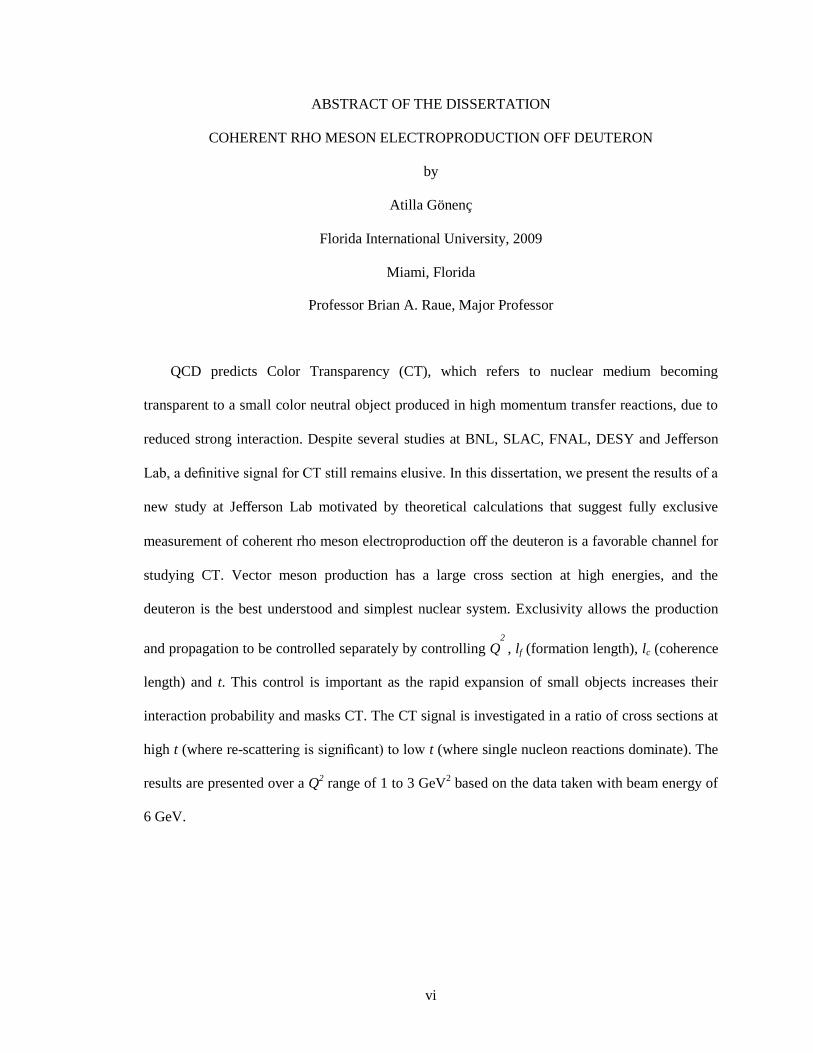
QCD predicts Color Transparency (CT), which refers to nuclear medium becoming
transparent to a small color neutral object produced in high momentum transfer reactions, due to
reduced strong interaction. Despite several studies at BNL, SLAC, FNAL, DESY and Jefferson
Lab, a definitive signal for CT still remains elusive. In this dissertation, we present the results of a
new study at Jefferson Lab motivated by theoretical calculations that suggest fully exclusive
measurement of coherent rho meson electroproduction off the deuteron is a favorable channel for
studying CT. Vector meson production has a large cross section at high energies, and the
deuteron is the best understood and simplest nuclear system. Exclusivity allows the production
and propagation to be controlled separately by controlling Q2
, lf (formation length), lc (coherence
length) and t. This control is important as the rapid expansion of small objects increases their
interaction probability and masks CT. The CT signal is investigated in a ratio of cross sections at
high t (where re-scattering is significant) to low t (where single nucleon reactions dominate). The
results are presented over a Q2 range of 1 to 3 GeV
2 based on the data taken with beam energy of
6 GeV.
vii
TABLE OF CONTENTS
CHAPTER PAGE
1 Theoretical Background and Motivation ................................................................................. 5 1.1 Color Transparency .......................................................................................................... 5 1.2 Basic Aspects of Color Transparency .............................................................................. 7 1.3 Coherent Vector Meson Production ................................................................................. 8 1.4 Experimental Objectives ................................................................................................ 11 1.5 Previous Data and Measurements .................................................................................. 13
1.5.1 Color Transparency in A(p,2p) .............................................................................. 13 1.5.2 Color Transparency in A(e,e’p) ............................................................................. 15 1.5.3 Color Transparency in A( , dijet) ........................................................................ 16
1.5.4 Color Transparency in A(', ) ......................................................................... 17
1.5.5 Color Transparency in A( , p ) .......................................................................... 18
1.5.6 Color Transparency in A( , ' )e e ....................................................................... 19
2 Experimental Setup ................................................................................................................ 22 2.1 Jefferson Lab .................................................................................................................. 22 2.2 CLAS Detector, Target, and Trigger ............................................................................. 23
3 Particle Identification and Event Selection ............................................................................ 26 3.1 Data Quality ................................................................................................................... 26 3.2 Corrections ..................................................................................................................... 30
3.2.1 Energy Loss and Momentum Corrections ............................................................. 30 3.2.2 Electron Beam Energy Correction ......................................................................... 34 3.2.3 Vertex correction ................................................................................................... 35
3.3 Particle Identification ..................................................................................................... 36 3.3.1 Scattered Electron Identification ............................................................................ 36 3.3.2 Hadron Identification ............................................................................................. 49
3.4 Additional Cuts .............................................................................................................. 56 3.4.1 Bad scintillator paddle removal ............................................................................. 56 3.4.2 W invariant mass cut .............................................................................................. 57
4 Yield Corrections, Extraction and Systematic Uncertainties ................................................. 59 4.1 Data Correction Factors ................................................................................................. 59
4.1.1 Acceptance ............................................................................................................. 59 4.1.2 Other Correction Factors ........................................................................................ 62
4.2 Data Normalization ........................................................................................................ 65 4.3 Yield Extraction ............................................................................................................. 67
4.3.1 Mass spectrum of the ρ particle ............................................................................. 67 4.3.2 The Fitting Method ................................................................................................ 68 4.3.3 Understanding the background .............................................................................. 70 4.3.4 Uncertainties .......................................................................................................... 72
5 Results and Discussions ......................................................................................................... 76 5.1 The Differential Cross Section ....................................................................................... 76 5.2 CT ratio .......................................................................................................................... 78
viii
5.3 Check of SCHC.............................................................................................................. 80 5.4 Ratio of longitudinal to tranverse cross section ............................................................. 81 5.5 Summary and Conclusions ............................................................................................ 85
REFERENCES .............................................................................................................................. 86
VITA .............................................................................................................................................. 89
ix
LIST OF FIGURES
FIGURE PAGE
1. Graphical representation of the rho electroproduction................................................................. 2
2. Graphical representation of coherence and formation lengths ..................................................... 4
3. Interaction probability of ultra-relativistic e e pairs. ................................................................ 6
4. Graphical representation of short and long formation length lf ................................................... 8
5. Graphical representation of short and long coherence length lc . ................................................. 8
6. Exclusive vector meson production ............................................................................................. 9
7. The photoproduction cross section of rho mesons. .................................................................... 10
8. The expected ratio RCT of the rho meson electroproduction cross sections. .............................. 11
9. Nuclear transparency measurement in reaction ( ,2 )A p p ........................................................ 14
10. Nuclear transparency measurements with'( , )A e e p experiments. .......................................... 15
11. The observed A dependence of diffractive dissociation into dijets ..................................... 16
12. The transparency T as a function of A, for three Q2 regions .................................................... 18
13. Nuclear transparency TA plotted as a function of coherence length lc ...................................... 19
14. Nuclear transparency as a function of Q2 ................................................................................. 20
15. The nuclear transparency of 4He .............................................................................................. 20
16. The extracted nuclear transparency T ...................................................................................... 21
17. A schematic diagram of CEBAF ............................................................................................. 22
18. A schematic diagram of CLAS showing various subsystems. ................................................. 23
19. E6 target cell. ........................................................................................................................... 25
20. Kinematic distributions of the data set used in the analysis..................................................... 26
21. Diagnostics plots for SC detector............................................................................................. 27
22. Diagnostics plots for EC detector ............................................................................................ 28

x
23. The time dependence of the DC residuals ............................................................................... 28
24. Number of deuterons and pions vs run number. ...................................................................... 29
25. Number of electrons vs run file number. ................................................................................. 30
26. Deuteron energy loss. ............................................................................................................... 31
27. Fit of pgen/prec vs prec for sector 1 .............................................................................................. 32
28. Missing mass squared distribution of edπ+ .............................................................................. 33
29. Beam energy ............................................................................................................................ 34
30. Gaussian fit to beam energy ..................................................................................................... 35
31. Variables used in vertex correction. ......................................................................................... 36
32. Electron Z-vertex (in cm), before and after the vertex correction ............................................ 37
33. CED display of an electron candidate ...................................................................................... 37
34. Electron Z vertex distribution .................................................................................................. 39
35. Two pion invariant mass distribution....................................................................................... 40
36. Sampling fraction vs. U, V and W ............................................................................................ 41
37. Azimuthal angle distribution versus polar angle of the electron .............................................. 43
38. Electron polar scattering angle vs momentum for sector 5 ...................................................... 44
39. Total energy and inner energy deposited in the calorimeter .................................................... 45
40. Photoelectron distribution for different momentum bins ......................................................... 46
41. edπ+ missing mass squared distribution ................................................................................... 47
42. Cerenkov photoelectron spectrum (black) ............................................................................... 48
43. Correction function used to account for pion contamination ................................................... 49
44. Hadron Z vertex distribution. ................................................................................................... 50
45. Distribution of υ vs θ ............................................................................................................... 51
46. β vs p for charged particles ...................................................................................................... 52
47. Kinetic energy distribution of identified deuterons. ................................................................ 53
xi
48. Missing mass squared (GeV2) distribution, for the ed ed X reaction. .......................... 54
49. Energy deposited (in MeV) in the TOF scintillator ................................................................. 54
50. Distribution of vertex time difference. ..................................................................................... 55
51. Electron time vertex plot versus scintillator paddle number .................................................... 56
52. W invariant distribution ............................................................................................................ 57
53. Missing mass squared (GeV2) .................................................................................................. 58
54. b as a function of Q2 in rho photo and electroproduction ........................................................ 60
55. Examples of some kinematic variables .................................................................................... 61
56. Top: Q2 dependence of acceptance for fixed lc ........................................................................ 63
57. The photoelectron distribution in the Cerenkov ...................................................................... 64
58. EC and CC efficiencies ............................................................................................................ 65
59. The virtual photon polarization ................................................................................................ 66
60. Reconstruction of the π+π
- final state ....................................................................................... 68
61. Invariant mass spectrum .......................................................................................................... 69
62. The background from misidentified deuterons ........................................................................ 70
63. M[edX] distribution for M2[edπ
+X] ≥ 0.1 GeV
2 ....................................................................... 71
64. Statistical error on the normalized yield .................................................................................. 73
65. Invariant Mass of π+π
- ............................................................................................................ 75
66. Normalized yield vs –t’ ............................................................................................................ 76
67. The invariant mass distributions .............................................................................................. 77
68. The t slope values vs lc for world ρ production on the proton ................................................. 78
69. Cross section ratios at different momentum transfers and fixed lc ........................................... 79
70. lf vs lc distribution for the E6 data ........................................................................................... 79
71. Phi distribution integrated over all kinematics. ....................................................................... 81
72. The invariant mass distributions in eight bins of phi. .............................................................. 82

xii
73. The invariant mass fits used to extract the yields in each cos(h) bin. ..................................... 83
74. Cosine projection, background subtracted and fitted ............................................................... 84
75. Ratio of longitudinal to transverse cross sections .................................................................... 84

xiii
LIST OF TABLES
FIGURE PAGE
1. Parameters used in deuteron energy loss correction .................................................................. 32
2. Cerenkov fiducial cut parameterization constants ..................................................................... 42
3. Parameters to exclude angular regions for Sectors 3, 5 and 6 ................................................... 44
4. Fir results on the invariant mass spectrum ................................................................................. 69
5. Table of systematic errors .......................................................................................................... 72

1
Notations
The electroproduction of rho vector mesons off a deuteron in a fully exclusive reaction can be
written as
' 'e d e d V (1)
which, with the assumption of only one virtual photon exchange, reduces to
* 'd d V (2)
The initial electron, characterized by the four-vector ( , )e ee E p
emits a virtual photon
* ( , )q
that interacts with the deuteron target ( ,0)dd M , which is at rest in the laboratory
frame, and produces a scattered deuteron ' ( , )d dd E p
and a rho vector meson ( , )V VV E p
in
the final state.
The virtual photon four-momentum can then be written in terms of the incident electron four-
momentum e and the scattered electron four-momentum 'e as
* 'e e (3)
where ' '
' ( , )e e
e E p
.
The negative square of the four-momentum of the virtual photon or the photon virtuality is given
by
'
2 2 * 2 ' 2 2 1( ) ( ) 4 sin ( )
2e ee
Q q e e E E (4)
where e is the lab-frame angle between incident and scattered electron‟s momentum vectors. In
this equation, the electron rest mass has been ignored due to its small size relative to the electron
momentum.
2
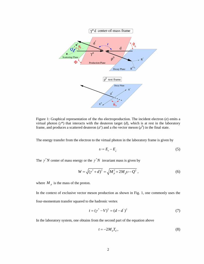
Figure 1: Graphical representation of the rho electroproduction. The incident electron (e) emits a
virtual photon (γ*) that interacts with the deuteron target (d), which is at rest in the laboratory
frame, and produces a scattered deuteron (d’) and a rho vector meson (ρ0) in the final state.
The energy transfer from the electron to the virtual photon in the laboratory frame is given by
'e eE E (5)
The *N center of mass energy or the
*N invariant mass is given by
* 2 2 2( ) 2p pW d M M Q , (6)
where pM is the mass of the proton.
In the context of exclusive vector meson production as shown in Fig. 1, one commonly uses the
four-momentum transfer squared to the hadronic vertex
* 2 ' 2( ) ( )t V d d (7)
In the laboratory system, one obtains from the second part of the equation above
2 d dt M T , (8)
3
which gives a simple expression for t as a function of the kinetic energy of the scattered target,
dT .
Another commonly used variable is t’ , which is defined as
/
mint t t (9)
where tmin is the minimum value of t kinematically necessary to put the rho and deuteron system
on shell.
Coherence length, cl , plays a very important role in the context of color transparency and is a
scale defined as
2 2
2cl
m Q
(10)
where m is the mass of the rho meson. It can be derived by applying the uncertainty principle
to the * vertex
1ct l E (11)
Assuming conservation of momentum p at the * vertex
2 2 2 2Q q p (12)
Then
1 2 1 2
2 2 2 2 2E E p M Q M (13)
At large
2 2 2 2
(1 ...)2 2
Q M Q ME
(14)
Then
4
2 2 2 2
1 21
2
cl EQ M Q M
(15)
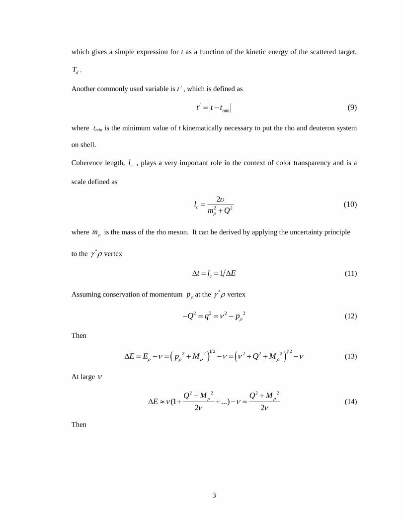
Another governing scale for the color transparency effect is the formation length, fl , defined [1]
as
2 2
22f
Ql
m
(16)
where 2 2( 0.7 1.0 GeV )m is the typical squared mass difference between the vector meson
ground state and the first excited state. The schematic diagram for these scales is shown in Fig. 2.
Figure 2: Graphical representation of coherence and formation lengths. The coherence length
defines a distance over which the photon fluctuates into a hadronic state and the formation length
describes the distance over which the intermediate hadronic states will expand and attain a normal
hadronic size.
5
1 Theoretical Background and Motivation
1.1 Color Transparency
Quantum Chromodynamics (QCD) is the universally accepted theory of strong interactions at
high energies. Its unique characteristic is that quarks and gluons, the ultimate constituents of
neutrons and protons, cannot exist as free particles: Two quarks interact more and more strongly
as they are pulled further apart. Fortunately, QCD includes asymptotic freedom in which the
interaction between quarks and gluons become weak at short distances. This leads to a
fundamental prediction of QCD, the existence of Color Transparency (CT).
The concept of CT was introduced independently by Brodsky and Mueller [2] in 1982,
and has since stimulated great interest. The basic idea behind CT is actually simple: When a
particle propagates through a nuclear medium, interactions occur that may lead to the absorption
of the propagating particle. Yet, if one could produce a very small size configuration of quarks
and gluons, it will interact weakly with nuclear medium and therefore it could pass undisturbed
through the nuclear medium. These small size configurations are referred to as Point Like
Configurations (PLCs).
CT: disappearance of the color forces between the hadrons and nuclei.
A similar phenomenon, known as Chudakov-Perkins effect [3], occurs in Quantum
Electrodynamics (QED): The interaction cross section of an electric dipole is proportional to the
square of its size. As a result, the cross section vanishes for objects with very small electric dipole
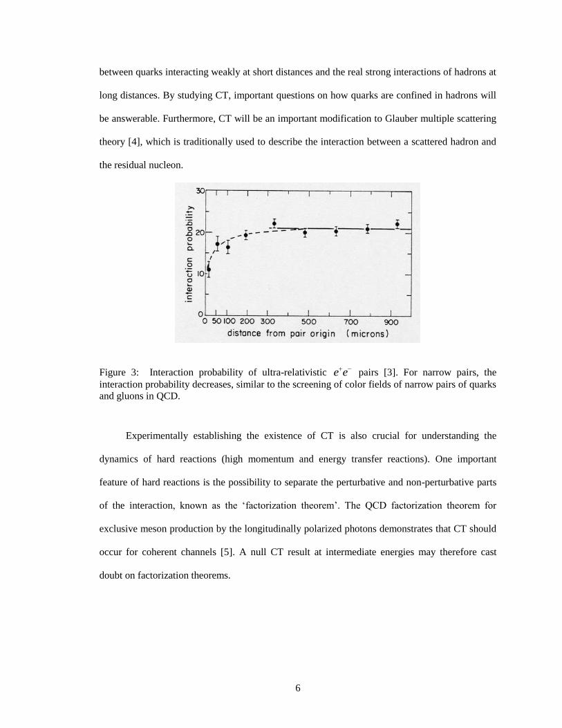
moments. This can be seen in Fig. 3, which shows the decreasing interaction probability for
narrow electron-positron pairs. Since color is the charge of QCD, in analogy to QED, the cross
section of a small color-neutral object is also predicted to vanish.
CT plays a central role in bridging the non-relativistic picture of nucleons making up a
nucleus and the ultra-relativistic perturbative approach used to establish QCD. It interpolates
6
between quarks interacting weakly at short distances and the real strong interactions of hadrons at
long distances. By studying CT, important questions on how quarks are confined in hadrons will
be answerable. Furthermore, CT will be an important modification to Glauber multiple scattering
theory [4], which is traditionally used to describe the interaction between a scattered hadron and
the residual nucleon.
Figure 3: Interaction probability of ultra-relativistic e e pairs [3]. For narrow pairs, the
interaction probability decreases, similar to the screening of color fields of narrow pairs of quarks
and gluons in QCD.
Experimentally establishing the existence of CT is also crucial for understanding the
dynamics of hard reactions (high momentum and energy transfer reactions). One important
feature of hard reactions is the possibility to separate the perturbative and non-perturbative parts
of the interaction, known as the „factorization theorem‟. The QCD factorization theorem for
exclusive meson production by the longitudinally polarized photons demonstrates that CT should
occur for coherent channels [5]. A null CT result at intermediate energies may therefore cast
doubt on factorization theorems.

7
1.2 Basic Aspects of Color Transparency
CT was first discussed in the context of perturbative QCD. This is certainly valid once one goes
to high enough energies (2 5 10Q GeV
2). However it is not clear exactly at what energies
energies this formalism will be applicable. Later work [6] indicates that the CT phenomenon also
occurs in a wide variety of model calculations with nonperturbative reaction mechanisms. In
general, observing CT first requires that a high-momentum-transfer scattering take place for the
PLC to form. This PLC should be color neutral in order not to radiate gluons and must maintain
its compact size for some distance in traversing the nuclear medium prior to its inevitable
expansion. It is inevitable because the PLC is not a physical state, but is a wave packet that
undergoes time evolution. Any evolution necessarily causes expansion as the PLC initially has no
size.
A commonly used observable to test CT effects is the “nuclear transparency ratio”
introduced by Carroll et al. [7]. It is defined as the ratio of a cross section measured in a nuclear
target to the analogous cross section for isolated hadrons in free space. If CT exists, one would
expect that hard scattering in the nuclear medium is the same as the free space scattering and that
the nucleus is indeed transparent to incoming and outgoing hadrons.
The signal for color transparency is then a monotonic rise in the transparency ratio
(vanishing final state interaction) with increasing hardness of the reaction, asymptotically
approaching one. However, one has to be careful about all the other effects that can imitate and/or
mask the CT signal (see Figs 4 and 5). In leptoproduction processes for instance, even though
small-sized wave packets may be produced at low values of 2Q , interactions are suppressed only
when formation length, fl , exceeds the nuclear radius AR . When this condition is violated, the
produced hadron expands rapidly within the nucleus, and the final state interaction is restored. If
formation length fl is comparable to the target size, then nuclear effects become important for
8
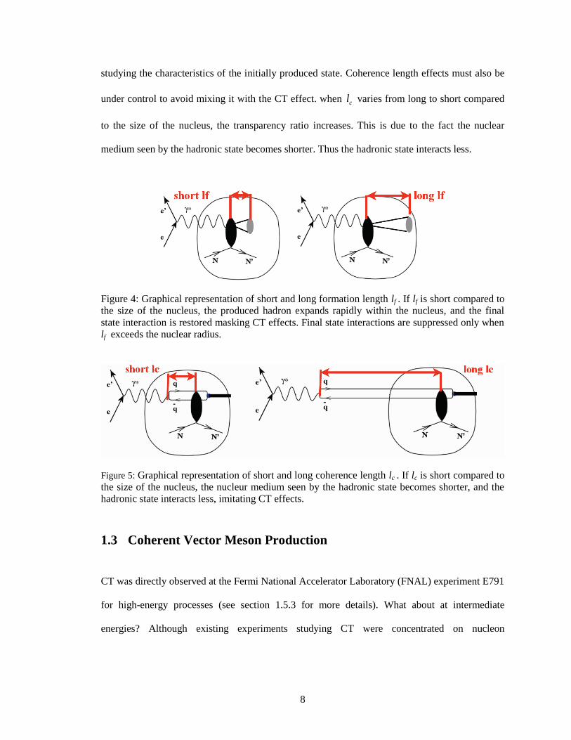
studying the characteristics of the initially produced state. Coherence length effects must also be
under control to avoid mixing it with the CT effect. when cl varies from long to short compared
to the size of the nucleus, the transparency ratio increases. This is due to the fact the nuclear
medium seen by the hadronic state becomes shorter. Thus the hadronic state interacts less.
Figure 4: Graphical representation of short and long formation length lf . If lf is short compared to
the size of the nucleus, the produced hadron expands rapidly within the nucleus, and the final
state interaction is restored masking CT effects. Final state interactions are suppressed only when
lf exceeds the nuclear radius.
Figure 5: Graphical representation of short and long coherence length lc . If lc is short compared to
the size of the nucleus, the nucleur medium seen by the hadronic state becomes shorter, and the
hadronic state interacts less, imitating CT effects.
1.3 Coherent Vector Meson Production
CT was directly observed at the Fermi National Accelerator Laboratory (FNAL) experiment E791
for high-energy processes (see section 1.5.3 for more details). What about at intermediate
energies? Although existing experiments studying CT were concentrated on nucleon
9
electroproduction, one should observe the onset of CT in meson electroproduction at lower values
of 2Q than nucleon knockout reactions. It should be easier to bring the quark and anti-quark of a
meson close together to form a PLC than the three quarks of a baryon [8], which makes meson
production an ideal choice to study CT.
The most promising channel for studying CT effects with meson electroproduction is the
coherent production of the rho meson off a deuteron target, ' 'e d e d , for the
following reasons:
Due to large photon-vector meson coupling, the cross section of the process is large, and,
at high energies and small Q2, is well understood in the framework of the vector meson
dominance (VMD) model.
The deuteron is the theoretically best-understood nucleus. It has zero isospin and as a
result, in the coherent channel, rho-omega mixing will be strongly suppressed, since the rho and
omega have isospin one and zero, respectively. This suppression allows one to not include the
rho-omega interference effects in the background. The technical advantage of using the deuteron
in coherent reactions is the possibility of detecting the recoil deuterons.
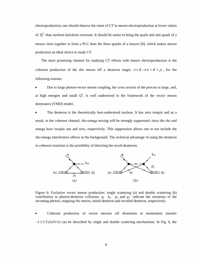
Figure 6: Exclusive vector meson production: single scattering (a) and double scattering (b)
contribution in photon-deuteron collisions. q, kv, pd and pd’ indicate the momenta of the
incoming photon, outgoing rho meson, initial deuteron and recoiled deuteron, respectively.
Coherent production of vector mesons off deuterium at momentum transfer
1.5t (GeV/c) can be described by single and double scattering mechanisms. In Fig. 6, the
10
schematic diagrams for these processes are shown. Fig. 6a corresponds to single scattering, where
only one nucleon participates in the interaction. Fig. 6b corresponds to the rescattering
mechanism, where the photon interacts with one of the nucleons inside the target, produces an
intermediate hadronic state that subsequently re-scatters from the second nucleon before forming
the final state vector meson. By studying rescattering, one can obtain a more detailed picture of
the PLC through its interaction with the nuclei.
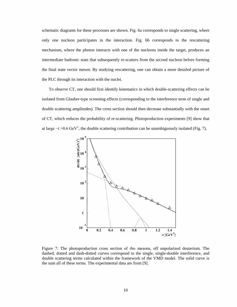
To observe CT, one should first identify kinematics in which double-scattering effects can be
isolated from Glauber-type screening effects (corresponding to the interference term of single and
double scattering amplitudes). The cross section should then decrease substantially with the onset
of CT, which reduces the probability of re-scattering. Photoproduction experiments [9] show that
at large −t >0.6 GeV2, the double scattering contribution can be unambiguously isolated (Fig. 7).
Figure 7: The photoproduction cross section of rho mesons, off unpolarized deuterium. The
dashed, dotted and dash-dotted curves correspond to the single, single-double interference, and
double scattering terms calculated within the framework of the VMD model. The solid curve is
the sum all of these terms. The experimental data are from [9].
11
1.4 Experimental Objectives
Ratio of differential cross sections:
In this dissertation, first the t dependence of the differential cross section will be studied
for a wide range in Q2 for -t up to 1 (GeV/c)
2. The focus however will be the ratio of differential
cross sections, measured at kinematics for which double scattering is dominant to the cross
section measured at kinematics where the effect of Glauber screening (single scattering) is more
important:
2
2
sin
( , , )
( , , )
c doubleCT
c gle
d Q l t dtR
d Q l t dt
(16)
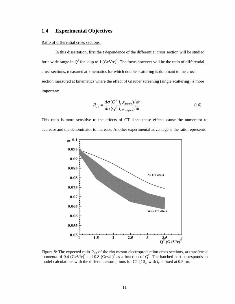
This ratio is more sensitive to the effects of CT since these effects cause the numerator to
decrease and the denominator to increase. Another experimental advantage is the ratio represents
Figure 8: The expected ratio RCT of the rho meson electroproduction cross sections, at transferred
momenta of 0.4 (GeV/c)2
and 0.8 (Gev/c)2 as a function of Q
2. The hatched part corresponds to
model calculations with the different assumptions for CT [10], with lc is fixed at 0.5 fm.
12
the ratio of quantities measured within the same experimental run. Therefore eliminating many of
the systematic uncertainties generally associated with absolute cross section measurements. This
ratio will then be compared to the theory.
In Fig. 8, a model calculation of the Q2
dependence of the ratio RCT for –t1=0.8 (GeV/c)2
and –t2=0.4 (GeV/c)2 is presented for rho electroproduction. The upper curve is calculated
without CT. The lower band corresponds to calculations with different assumptions for CT [10].
The coherence length is fixed at lc=0.5 fm. As one can see, already at Q2 = 3.5 (GeV/c)2 the
expected effect is in the 10%-15% range.
We will get the ed ed cross section from the data through
3
2 2
ed w
c c
d n
dQ dl dt Q l t
(17)
where nw is the acceptance, efficiency and radiative-correction weighted yield (number of
events) in each kinematic bin. The number of will be extracted from the integral of the
invariant mass histogram after background subtraction and phenomenological fits
explained in subsequent sections.
Angular distributions:
As a side product of this dissertation, we will study the decay angular distributions of the rho
mesons to investigate their spin structures and to separate the longitudinal and transverse
polarization. S-channel helicity conservation (SCHC) hypothesizes that the polarization of the rho
meson is equal to the polarization of the virtual photon, and its validitiy can be checked by
studying those decay density matrix elements that vanish in the case of SCHC. The rho meson
polarization state can be fully described by the spin density matrix which consists of 15
independent elements [11]. Assuming SHCH, 8 of 15 matrix elements become null and 3 are
independent. The rho meson angular distribution can then be expressed as a function of these
13
matrix elements. In particular, when integrated over the azimuthal angle, the decay angular
distribution in the helicity frame is given by
04 04 2
00 00
3(cos ) {1 (3 1)cos }
4h hW r r (18)
Assuming SCHC, the vector meson polarization can be linked to the virtual photon
polarization using the diagonal matrix element 04
00r which represents the fraction of longitudinal
by
04
00
04
00(1 )
L
T
rR
r
(19)
We will then compare our result with the previous electroproduction results that used a proton
target.
1.5 Previous Data and Measurements
1.5.1 Color Transparency in A(p,2p)
The first attempt to observe CT effects was made at Brookhaven National Laboratory (BNL) by
Carroll [7] with the ( ,2 )A p p reaction. The nuclear transparency was defined as the ratio of the
quasielastic cross section in a nuclear target to the analogous free pp cross section. The CT
prediction implies that for fast protons there will be a large decrease in final state interactions and
thus one should observe a dramatic increase in the transparency as a function of momentum
transfer squared. The experiment seemed to support a rise of transparency for incident beam
energies up to 9 GeV, but the surprising result was the significant drop in transparency with
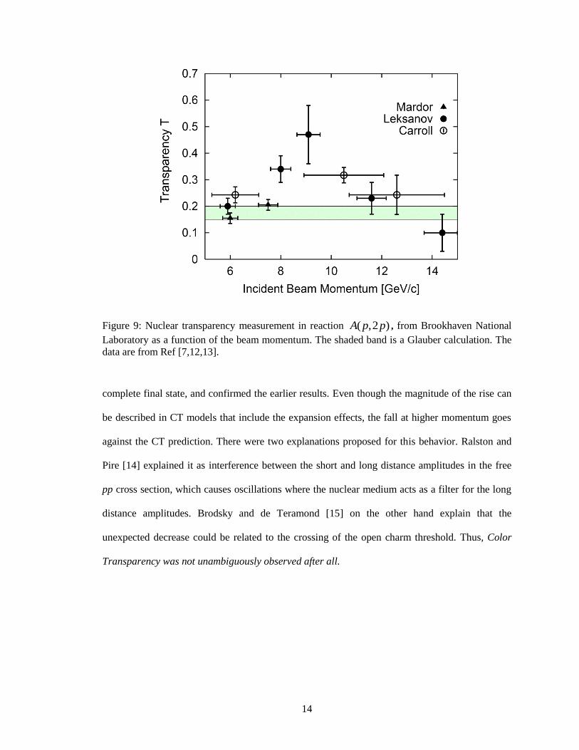
further increase of momentum (see Fig. 9).
There were some questions about the interpretation of these data: Since only one of the
two final-state protons was momentum analyzed, the exclusivity of the reaction could not be
guaranteed. A repeat of the experiment by Mardor [12] and later by Leksanov [13] did measure a
14
Figure 9: Nuclear transparency measurement in reaction ( ,2 )A p p , from Brookhaven National
Laboratory as a function of the beam momentum. The shaded band is a Glauber calculation. The
data are from Ref [7,12,13].
complete final state, and confirmed the earlier results. Even though the magnitude of the rise can
be described in CT models that include the expansion effects, the fall at higher momentum goes
against the CT prediction. There were two explanations proposed for this behavior. Ralston and
Pire [14] explained it as interference between the short and long distance amplitudes in the free
pp cross section, which causes oscillations where the nuclear medium acts as a filter for the long
distance amplitudes. Brodsky and de Teramond [15] on the other hand explain that the
unexpected decrease could be related to the crossing of the open charm threshold. Thus, Color
Transparency was not unambiguously observed after all.
15
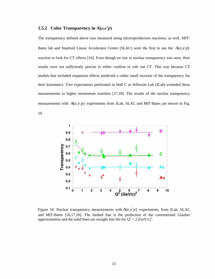
1.5.2 Color Transparency in A(e,e’p)
The transparency defined above was measured using electroproduction reactions, as well. MIT-
Bates lab and Stanford Linear Accelerator Center (SLAC) were the first to use the '( , )A e e p
reaction to look for CT effects [16]. Even though no rise in nuclear transparency was seen, their
results were not sufficiently precise to either confirm or rule out CT. This was because CT
models that included expansion effects predicted a rather small increase of the transparency for
their kinematics. Two experiments performed in Hall C at Jefferson Lab (JLab) extended these
measurements to higher momentum transfers [17,18]. The results of the nuclear transparency
measurements with '( , )A e e p experiments from JLab, SLAC and MIT-Bates are shown in Fig.
10.
Figure 10: Nuclear transparency measurements with'( , )A e e p experiments, from JLab, SLAC
and MIT-Bates [16,17,18]. The dashed line is the prediction of the conventional Glauber
approximation and the solid lines are straight line fits for Q2 > 2 (GeV/c)
2.

16
It is clear that the transparency is independent of 2Q up to 8.1 (GeV/c)
2 and the results agree with
the expectations of conventional nuclear physics, calculated by Pandharipande et al. [19] using a
Glauber approximation. It should be noted that at 2Q = 8 (GeV/c)
2 the momentum of the proton
ejected in electron scattering is about 5 GeV/c which is lower than the lowest momentum of 6
GeV/c used at BNL. One needs to achieve a 2Q of about 12 (GeV/c)
2 to reach a nucleon
momentum for which the BNL experiment observed an increase of the transparency.
1.5.3 Color Transparency in A( , dijet)
CT was directly observed at the Fermi National Accelerator Laboratory (FNAL) experiment
E791, which investigated the exclusive coherent production of two jets in the process
two jetsA A using 500 GeV/c pions on carbon and platinum targets [20]. The per-
nucleus cross section was parameterized as 0 A and the observed A-dependence of the
process was very different than typical 2 3A dependence of inclusive p-nucleus scattering.
Figure 11: The observed A dependence of diffractive dissociation into dijets, from FNAL for
different values of jet transverse momentum kT. The result was consistent with the theoretical
predictions, indicating a clear observation of CT at high energies. The data are from Ref [13].
17
As shown in Fig. 11, had values near 1.6, the exact result depending on jet transverse
momentum, and was consistent with the predictions of CT [21-23]. Thus, CT was observed at
high energies.
1.5.4 Color Transparency in A( ', )
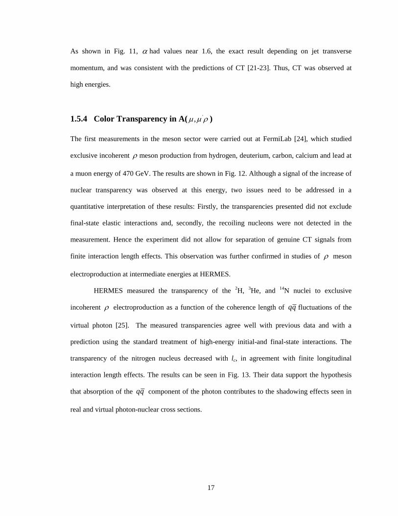
The first measurements in the meson sector were carried out at FermiLab [24], which studied
exclusive incoherent meson production from hydrogen, deuterium, carbon, calcium and lead at
a muon energy of 470 GeV. The results are shown in Fig. 12. Although a signal of the increase of
nuclear transparency was observed at this energy, two issues need to be addressed in a
quantitative interpretation of these results: Firstly, the transparencies presented did not exclude
final-state elastic interactions and, secondly, the recoiling nucleons were not detected in the
measurement. Hence the experiment did not allow for separation of genuine CT signals from
finite interaction length effects. This observation was further confirmed in studies of meson
electroproduction at intermediate energies at HERMES.
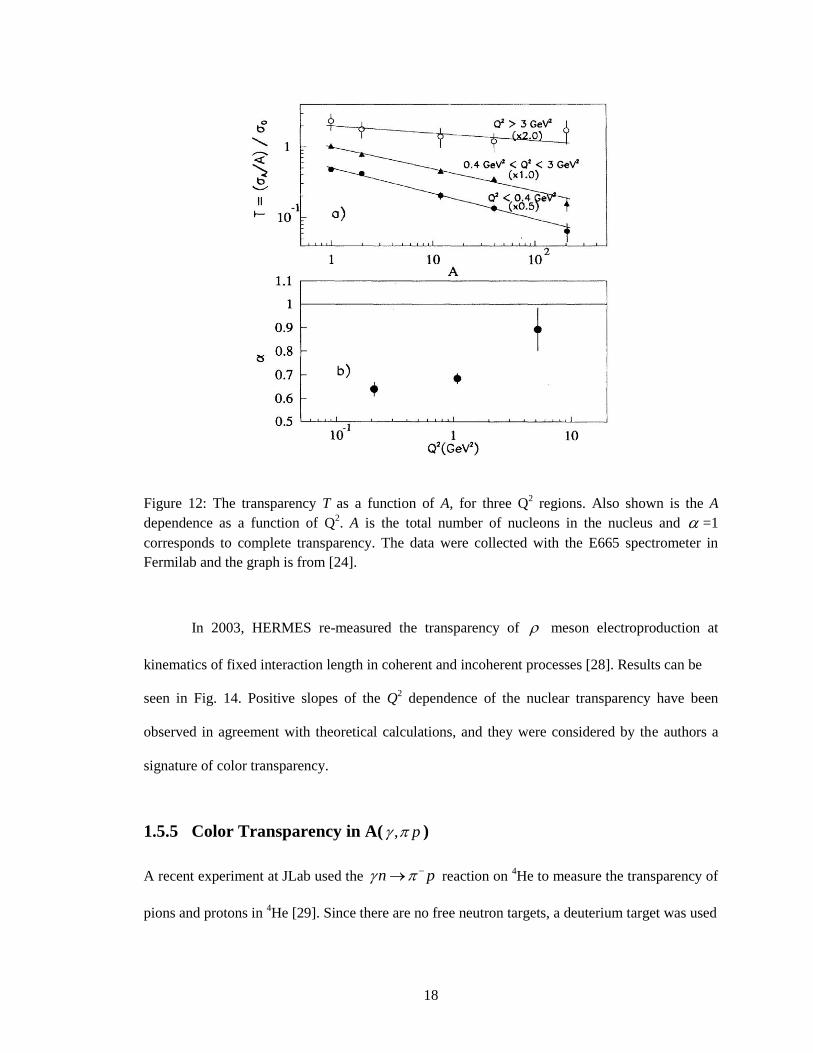
HERMES measured the transparency of the 2H,
3He, and
14N nuclei to exclusive
incoherent electroproduction as a function of the coherence length of qq fluctuations of the
virtual photon [25]. The measured transparencies agree well with previous data and with a
prediction using the standard treatment of high-energy initial-and final-state interactions. The
transparency of the nitrogen nucleus decreased with lc, in agreement with finite longitudinal
interaction length effects. The results can be seen in Fig. 13. Their data support the hypothesis
that absorption of the qq component of the photon contributes to the shadowing effects seen in
real and virtual photon-nuclear cross sections.
18
Figure 12: The transparency T as a function of A, for three Q2 regions. Also shown is the A
dependence as a function of Q2. A is the total number of nucleons in the nucleus and =1
corresponds to complete transparency. The data were collected with the E665 spectrometer in
Fermilab and the graph is from [24].
In 2003, HERMES re-measured the transparency of meson electroproduction at
kinematics of fixed interaction length in coherent and incoherent processes [28]. Results can be
seen in Fig. 14. Positive slopes of the Q2 dependence of the nuclear transparency have been
observed in agreement with theoretical calculations, and they were considered by the authors a
signature of color transparency.
1.5.5 Color Transparency in A( , p )
A recent experiment at JLab used the n p reaction on 4He to measure the transparency of
pions and protons in 4He [29]. Since there are no free neutron targets, a deuterium target was used
19
Figure 13: Nuclear transparency TA plotted as a function of coherence length lc , for rho
production on 2H,
3He, and
14N targets from reference [25]. Graph (c) includes comparisons with
previous experiments with photon (open diamonds) [26] and muon (open circle) [24] beams and
the dashed curves are the Glauber calculation from [27].
and a correction for the deuterium transparency was applied. The extracted nuclear transparency
for the 4He target along with calculations is shown in Fig. 15. The traditional nuclear physics
calculation appears to deviate from the data at the higher energies. However, the background
from multiple interactions was not controlled very well.
1.5.6 Color Transparency in A( , ' )e e
In a recent experiment at JLab [30], the nuclear transparency of pions in the reaction
A( , ' )e e was measured from
1H,
2H,
12C,
63Cu and
197Au targets at Q
2 of 1.1, 2.15, 3.0, 3.9, and
20
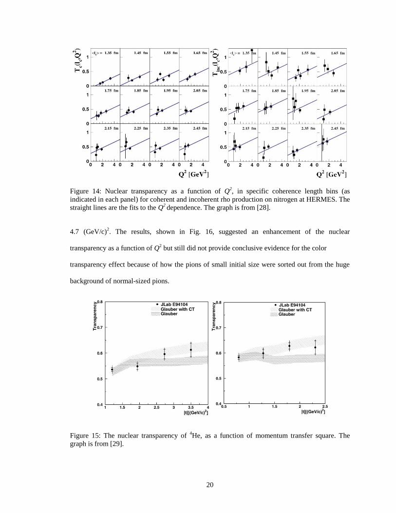
Figure 14: Nuclear transparency as a function of Q2, in specific coherence length bins (as
indicated in each panel) for coherent and incoherent rho production on nitrogen at HERMES. The
straight lines are the fits to the Q2 dependence. The graph is from [28].
4.7 (GeV/c)2. The results, shown in Fig. 16, suggested an enhancement of the nuclear
transparency as a function of Q2 but still did not provide conclusive evidence for the color
transparency effect because of how the pions of small initial size were sorted out from the huge
background of normal-sized pions.
Figure 15: The nuclear transparency of 4He, as a function of momentum transfer square. The
graph is from [29].
21
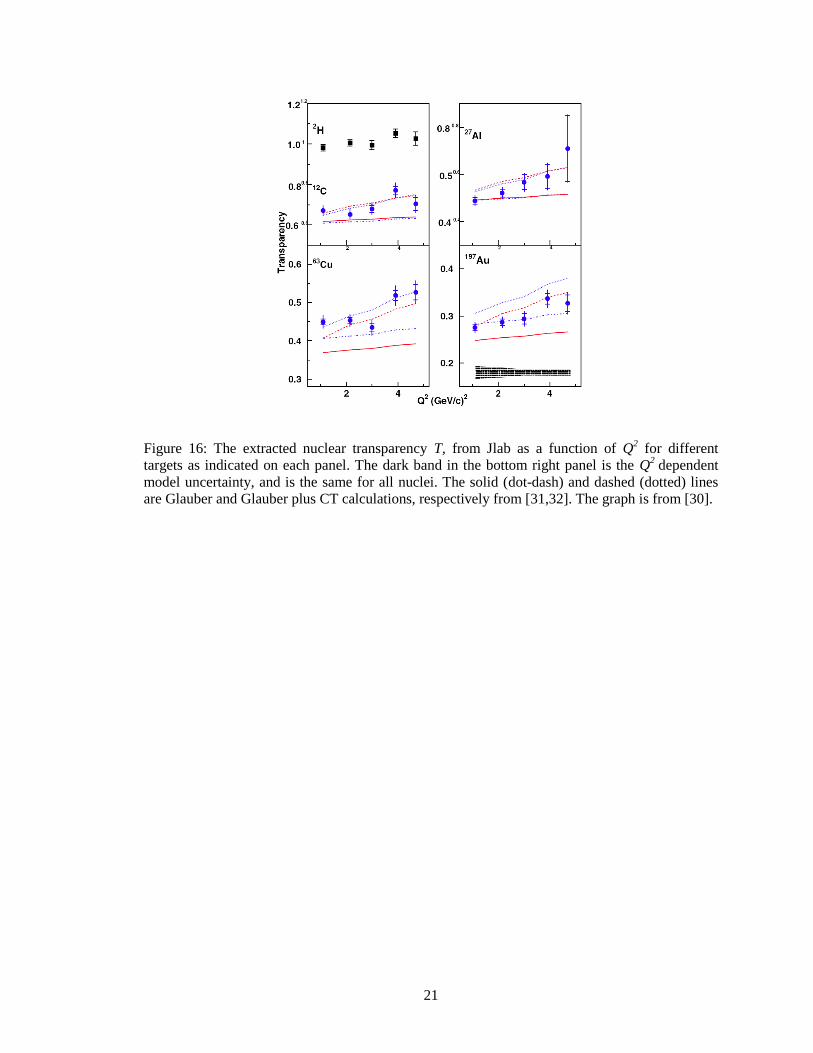
Figure 16: The extracted nuclear transparency T, from Jlab as a function of Q2 for different
targets as indicated on each panel. The dark band in the bottom right panel is the Q2
dependent
model uncertainty, and is the same for all nuclei. The solid (dot-dash) and dashed (dotted) lines
are Glauber and Glauber plus CT calculations, respectively from [31,32]. The graph is from [30].
22
2 Experimental Setup
2.1 Jefferson Lab
The data for this thesis comes from an experiment conducted at the Thomas Jefferson National
Accelerator Facility (JLab) in Newport News, Virginia, which is designed to perform research in
nuclear physics at intermediate energies using electromagnetic probes. This facility contains an
electron accelerator (CEBAF) that operates with superconducting RF cavities to drive the
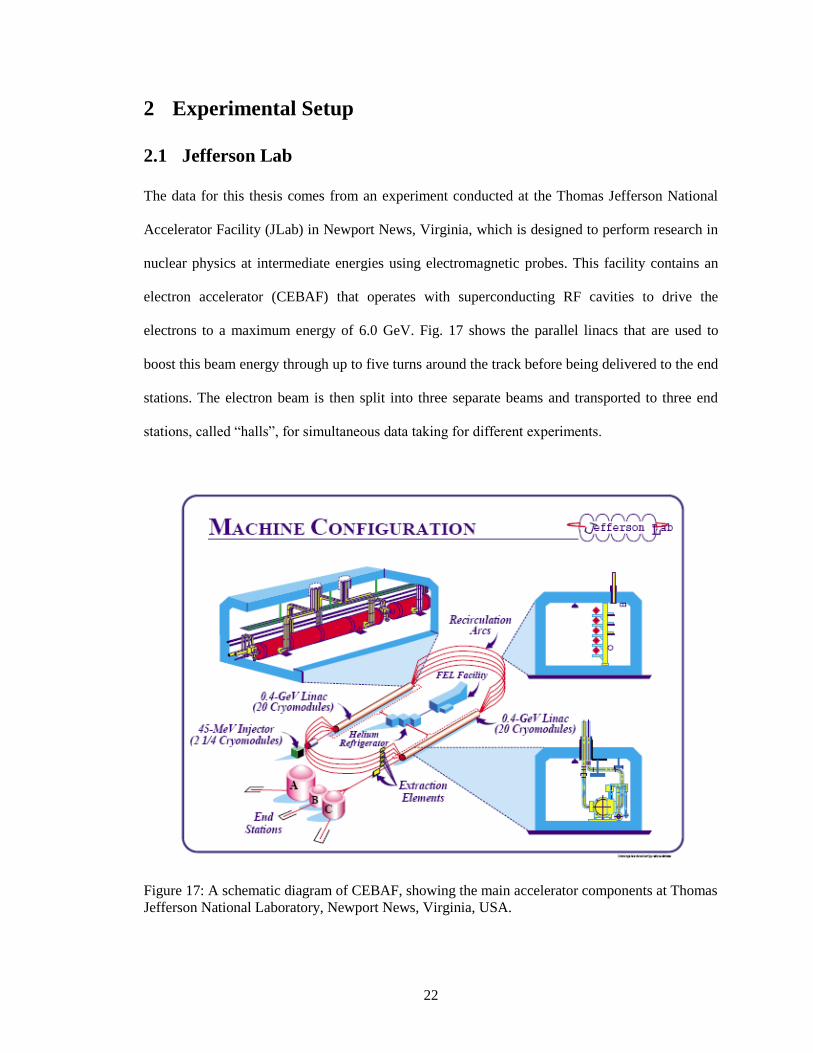
electrons to a maximum energy of 6.0 GeV. Fig. 17 shows the parallel linacs that are used to
boost this beam energy through up to five turns around the track before being delivered to the end
stations. The electron beam is then split into three separate beams and transported to three end
stations, called “halls”, for simultaneous data taking for different experiments.
Figure 17: A schematic diagram of CEBAF, showing the main accelerator components at Thomas
Jefferson National Laboratory, Newport News, Virginia, USA.

23
2.2 CLAS Detector, Target, and Trigger
The data were collected using the CEBAF Large Acceptance Spectrometer (CLAS) detector
system in Hall B (see Fig. 18) and has been well documented elsewhere [33]. In this section,
only special conditions for this experiment along with the general layout of the CLAS detector,
data acquisition, and trigger are presented.
CLAS is based around six iron-free superconducting coils centered on the beam line to
create a toroidal magnetic field that can be adjusted up to 2 Tesla, with a maximum field integral
of 2.5 Tesla-meter in the forward direction. These six coils divide CLAS into six azimuthal
sectors each containing three multilayer drift chambers (DC) [34] that are used to determine the
trajectories and momenta of charged particles produced from a fixed target on the toroidal axis.
Figure 18: A schematic diagram of CLAS showing various subsystems.
24
Region 1 of the drift chambers is closest to target and beam line and operates in a region
with almost no magnetic field. This region is used to determine the initial trajectory of charged
particles. Region 2 drift chambers are located inside the strong magnetic field between the torus
coils and are used to obtain a measurement of the particle track at a point of maximum curvature.
Region 3 drift chambers rest outside the torus coils in a low magnetic field area and are used to
further determine the trajectory of charged particles before they hit other detector parts. The
time-of-flight (TOF) counters [35] are used to measure the time of flight of the particles, which is
combined with the momentum and path-length information from the drift chambers to determine
particle mass. The forward electromagnetic calorimeter (EC) [36] measures the energy of
electrons and high-energy neutral particles and provides for electron/pion separation. A gas filled
threshold Cerenkov counter [37] provides for electron/pion separation. Finally, the large angle
calorimeter (LAC), covering only two sectors, are used for detecting the photons coming from the
decay of neutral pions and etas.
The Level 1 trigger of the CLAS data acquisition (DAQ) consisted of a coincidence
between the Cherenkov counter (with a 100 mV trigger setup corresponding to at least 1 photo-
electron) and the electromagnetic calorimeter (with a 172 mV trigger setting corresponding to 0.5
GeV). A level 2 trigger, which requires a track candidate in the drift chambers in the same sector
of the calorimeter hit, was also used.
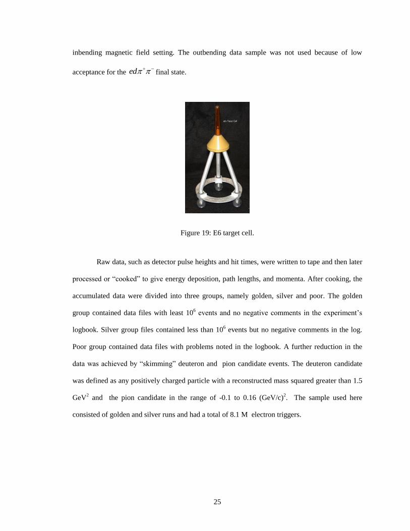
For this experiment, the target cell (Fig. 19) was filled with liquid deuterium and
positioned in the center of CLAS. The physical length of the target cell was 5 cm and at nominal
temperature of 22 K and pressure of 1315 mbar, the density was 0.162 g/cm3.
The data were collected during e6 run period in Hall B from January 30th till March 16
th,
2002. A polarized electron beam with energy of 5.75 GeV and an average current of 8 nA was
used. The data were collected at two different configurations of the magnetic field resulting in
inbending or outbending electrons. This dissertation covers only the data taken with the standard,
25
inbending magnetic field setting. The outbending data sample was not used because of low
acceptance for the ed final state.
Figure 19: E6 target cell.
Raw data, such as detector pulse heights and hit times, were written to tape and then later
processed or “cooked” to give energy deposition, path lengths, and momenta. After cooking, the
accumulated data were divided into three groups, namely golden, silver and poor. The golden
group contained data files with least 106 events and no negative comments in the experiment‟s
logbook. Silver group files contained less than 106 events but no negative comments in the log.
Poor group contained data files with problems noted in the logbook. A further reduction in the
data was achieved by “skimming” deuteron and pion candidate events. The deuteron candidate
was defined as any positively charged particle with a reconstructed mass squared greater than 1.5
GeV2 and the pion candidate in the range of -0.1 to 0.16 (GeV/c)
2. The sample used here
consisted of golden and silver runs and had a total of 8.1 M electron triggers.
26
3 Particle Identification and Event Selection
The main reaction studied for this thesis was the electroproduction of the rho vector meson off a
deuteron in the fully exclusive reaction, ed ed , where the ρ meson decays into two pions
almost 100% of the time according to Ref. [38]. To select coherent rho meson production events,
we first identified the scattered electron and scattered deuteron, and one of the decay pions. The
undetected pion was reconstructed by a missing mass technique. Rho reconstruction using the
invariant mass of ( ) will be presented in the next chapter.
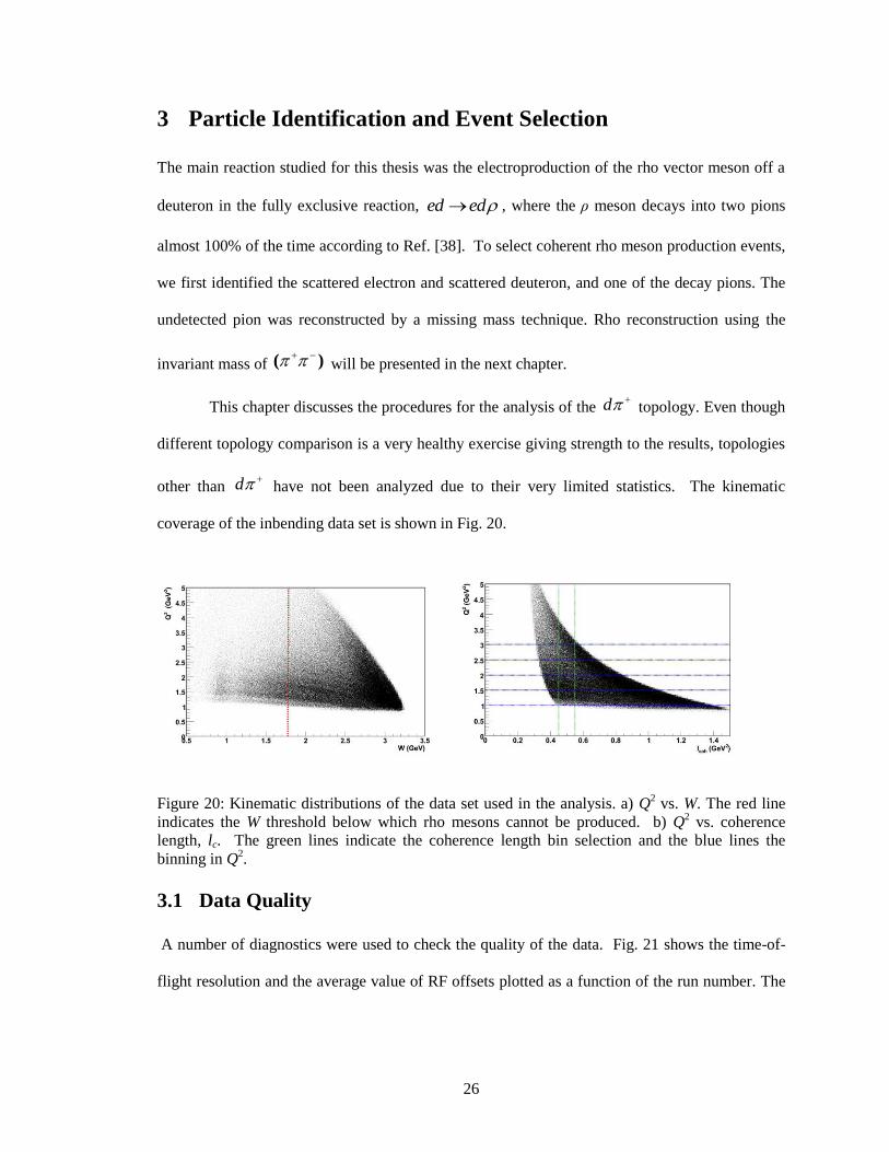
This chapter discusses the procedures for the analysis of the d topology. Even though
different topology comparison is a very healthy exercise giving strength to the results, topologies
other than d
have not been analyzed due to their very limited statistics. The kinematic
coverage of the inbending data set is shown in Fig. 20.
Figure 20: Kinematic distributions of the data set used in the analysis. a) Q2 vs. W. The red line
indicates the W threshold below which rho mesons cannot be produced. b) Q2 vs. coherence
length, lc. The green lines indicate the coherence length bin selection and the blue lines the
binning in Q2.
3.1 Data Quality
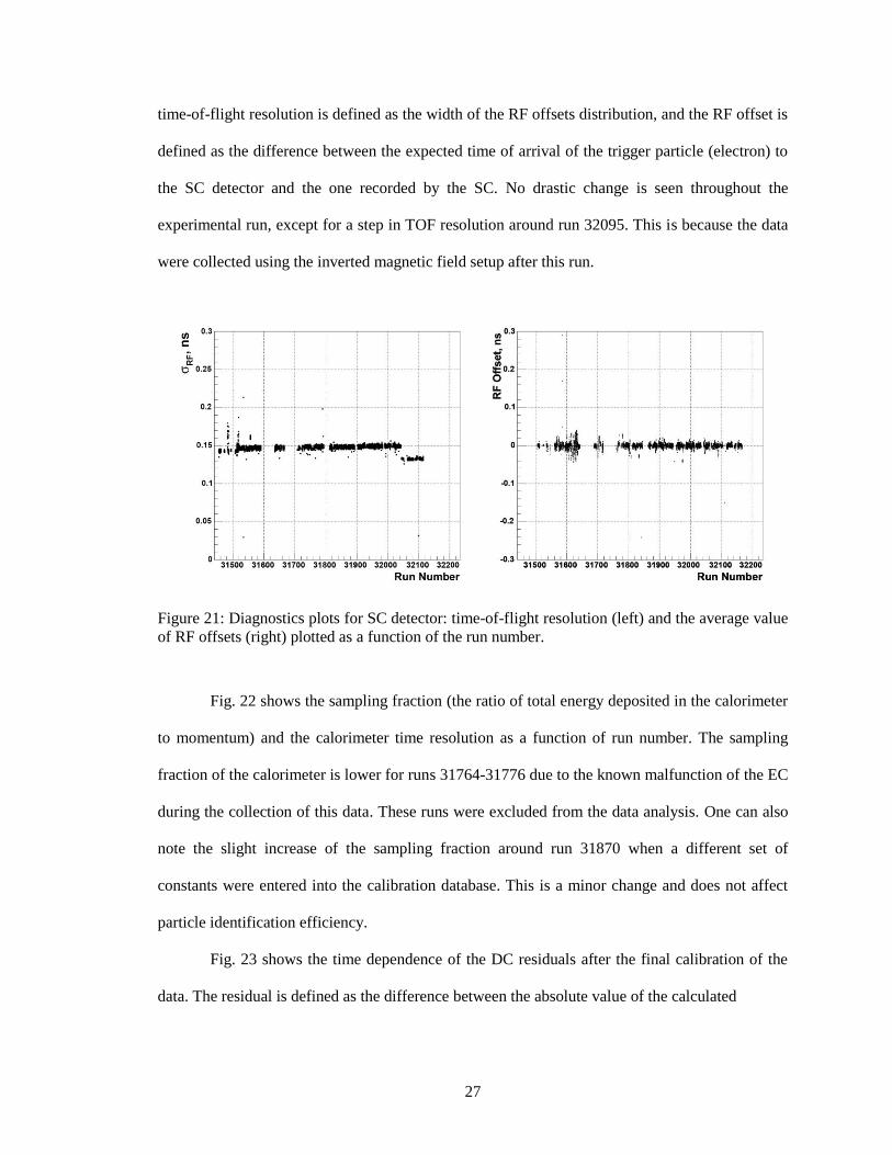
A number of diagnostics were used to check the quality of the data. Fig. 21 shows the time-of-
flight resolution and the average value of RF offsets plotted as a function of the run number. The
27
time-of-flight resolution is defined as the width of the RF offsets distribution, and the RF offset is
defined as the difference between the expected time of arrival of the trigger particle (electron) to
the SC detector and the one recorded by the SC. No drastic change is seen throughout the
experimental run, except for a step in TOF resolution around run 32095. This is because the data
were collected using the inverted magnetic field setup after this run.
Figure 21: Diagnostics plots for SC detector: time-of-flight resolution (left) and the average value
of RF offsets (right) plotted as a function of the run number.
Fig. 22 shows the sampling fraction (the ratio of total energy deposited in the calorimeter
to momentum) and the calorimeter time resolution as a function of run number. The sampling
fraction of the calorimeter is lower for runs 31764-31776 due to the known malfunction of the EC
during the collection of this data. These runs were excluded from the data analysis. One can also
note the slight increase of the sampling fraction around run 31870 when a different set of
constants were entered into the calibration database. This is a minor change and does not affect
particle identification efficiency.
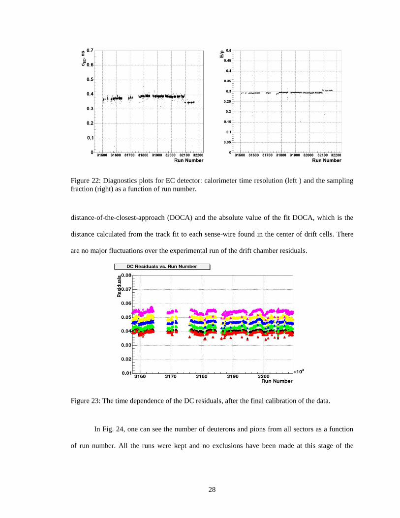
Fig. 23 shows the time dependence of the DC residuals after the final calibration of the
data. The residual is defined as the difference between the absolute value of the calculated
28
Figure 22: Diagnostics plots for EC detector: calorimeter time resolution (left ) and the sampling
fraction (right) as a function of run number.
distance-of-the-closest-approach (DOCA) and the absolute value of the fit DOCA, which is the
distance calculated from the track fit to each sense-wire found in the center of drift cells. There
are no major fluctuations over the experimental run of the drift chamber residuals.
Figure 23: The time dependence of the DC residuals, after the final calibration of the data.
In Fig. 24, one can see the number of deuterons and pions from all sectors as a function
of run number. All the runs were kept and no exclusions have been made at this stage of the
29
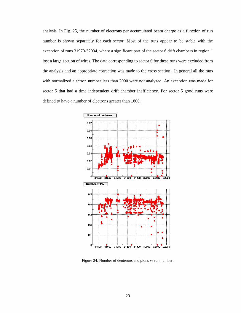
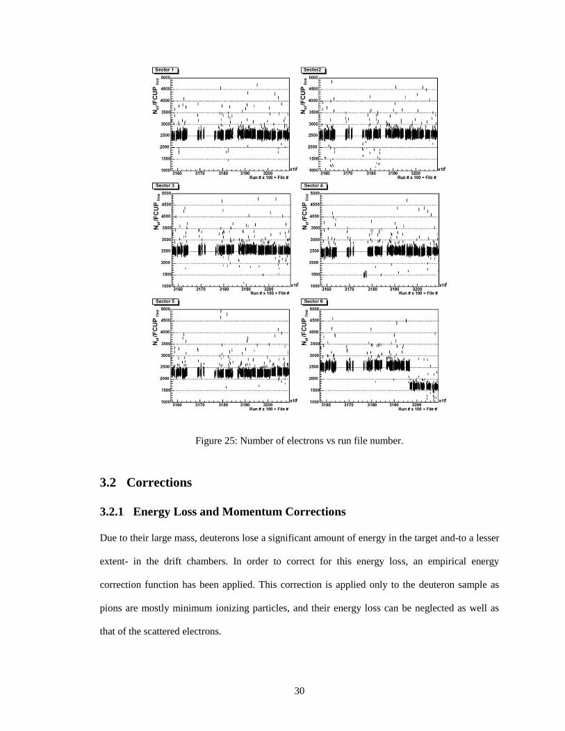
analysis. In Fig. 25, the number of electrons per accumulated beam charge as a function of run
number is shown separately for each sector. Most of the runs appear to be stable with the
exception of runs 31970-32094, where a significant part of the sector 6 drift chambers in region 1
lost a large section of wires. The data corresponding to sector 6 for these runs were excluded from
the analysis and an appropriate correction was made to the cross section. In general all the runs
with normalized electron number less than 2000 were not analyzed. An exception was made for
sector 5 that had a time independent drift chamber inefficiency. For sector 5 good runs were
defined to have a number of electrons greater than 1800.
Figure 24: Number of deuterons and pions vs run number.
30
Figure 25: Number of electrons vs run file number.
3.2 Corrections
3.2.1 Energy Loss and Momentum Corrections
Due to their large mass, deuterons lose a significant amount of energy in the target and-to a lesser
extent- in the drift chambers. In order to correct for this energy loss, an empirical energy
correction function has been applied. This correction is applied only to the deuteron sample as
pions are mostly minimum ionizing particles, and their energy loss can be neglected as well as
that of the scattered electrons.
31
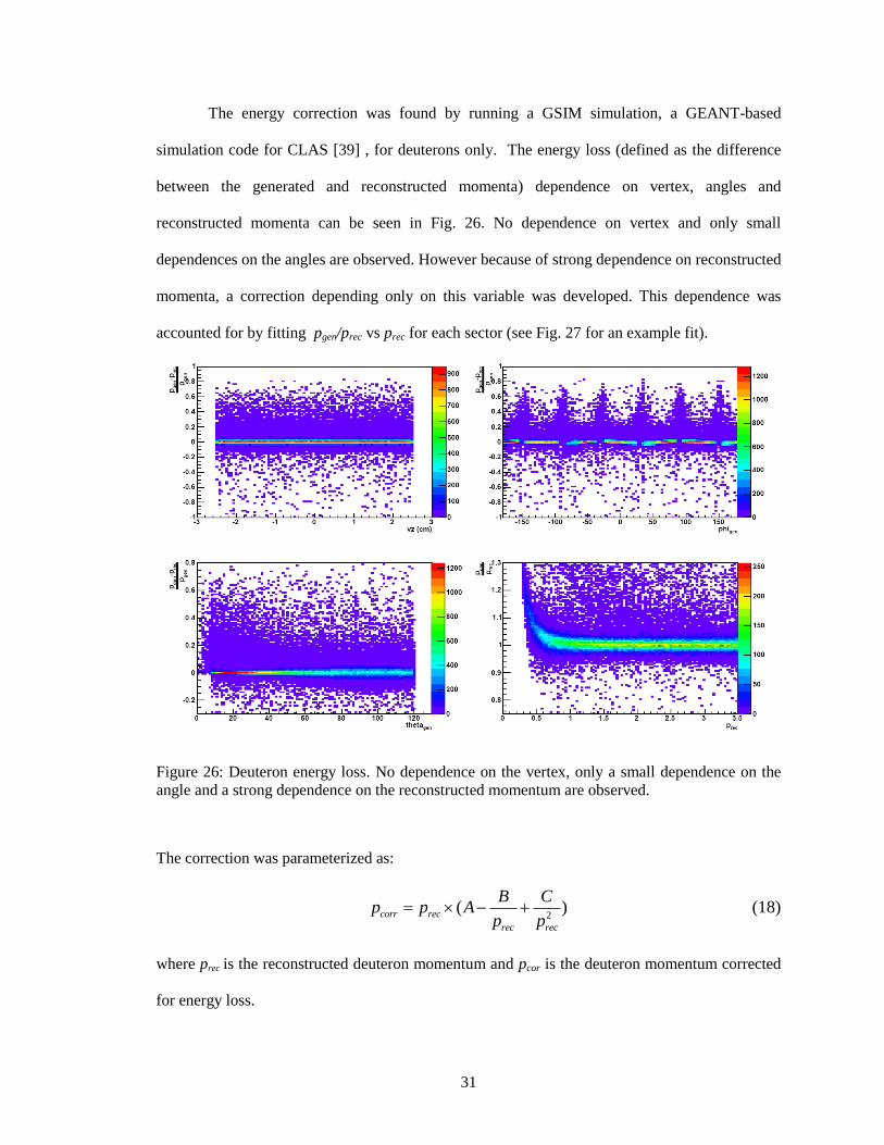
The energy correction was found by running a GSIM simulation, a GEANT-based
simulation code for CLAS [39] , for deuterons only. The energy loss (defined as the difference
between the generated and reconstructed momenta) dependence on vertex, angles and
reconstructed momenta can be seen in Fig. 26. No dependence on vertex and only small
dependences on the angles are observed. However because of strong dependence on reconstructed
momenta, a correction depending only on this variable was developed. This dependence was
accounted for by fitting pgen/prec vs prec for each sector (see Fig. 27 for an example fit).
Figure 26: Deuteron energy loss. No dependence on the vertex, only a small dependence on the
angle and a strong dependence on the reconstructed momentum are observed.
The correction was parameterized as:
2
( )corr rec
rec rec
B Cp p A
p p (18)
where prec is the reconstructed deuteron momentum and pcor is the deuteron momentum corrected
for energy loss.

32
Figure 27: Fit of pgen/prec vs prec for sector 1. The black crosses represent the profile histogram
from the data and the red line represents the fit to the profile histogram.
The parameters, which are sector dependent, are given in Table 1. Results have been checked by
studying the missing mass squared distribution of ede’d+(
-). After the corrections, the
dependence of the missing mass on the deuteron kinetic energy is removed as shown in Fig. 28.
Parameter sector 1 sector 2 sector 3 sector 4 sector 5 sector 6
A 1.01185 1.01301 1.01422 1.01184 1.00867 1.01845
B 0.0325639 0.0346238 0.0343279 0.0332074 0.0264245 0.0436208
C 0.0282014 0.0289473 0.0279420 0.0279010 0.0252732 0.0317149
Table 1: Parameters used in deuteron energy loss correction
Additional corrections were applied to correct for the systematic errors arising from
uncertainties in the knowledge of the torus magnetic field in each point of CLAS as well as of the
exact position of the drift chambers. These corrections depend on the particle‟s angle,
momentum, and mass, as well as the torus field. These corrections are typically less than 1% for
most kinematics and runs using specific DC alignment software. The details of the correction
algorithm can be found at [40]. This correction algorithm simultaneously corrects momenta and
polar angles of all final-state particles. The plot a) and b) in Fig. 28 shows the missing mass
squared distribution of edπ+
before and after the momentum corrections. As anticipated, the
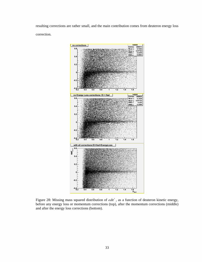
33
resulting corrections are rather small, and the main contribution comes from deuteron energy loss
correction.
Figure 28: Missing mass squared distribution of edπ+
, as a function of deuteron kinetic energy,
before any energy loss or momentum corrections (top), after the momentum corrections (middle)
and after the energy loss corrections (bottom).
34
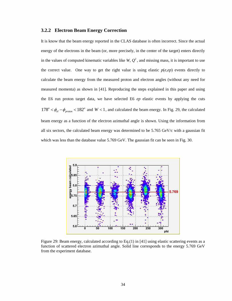
3.2.2 Electron Beam Energy Correction
It is know that the beam energy reported in the CLAS database is often incorrect. Since the actual
energy of the electrons in the beam (or, more precisely, in the center of the target) enters directly
in the values of computed kinematic variables like W, Q2 , and missing mass, it is important to use
the correct value. One way to get the right value is using elastic p(e,ep) events directly to
calculate the beam energy from the measured proton and electron angles (without any need for
measured momenta) as shown in [41]. Reproducing the steps explained in this paper and using
the E6 run proton target data, we have selected E6 ep elastic events by applying the cuts
178 182o o
el proton and 1W , and calculated the beam energy. In Fig. 29, the calculated
beam energy as a function of the electron azimuthal angle is shown. Using the information from
all six sectors, the calculated beam energy was determined to be 5.765 GeV/c with a gaussian fit
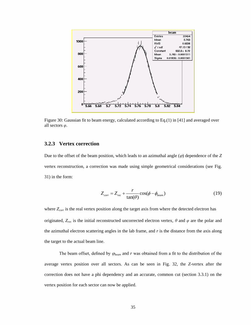
which was less than the database value 5.769 GeV. The gaussian fit can be seen in Fig. 30.
Figure 29: Beam energy, calculated according to Eq.(1) in [41] using elastic scattering events as a
function of scattered electron azimuthal angle. Solid line corresponds to the energy 5.769 GeV
from the experiment database.
35
Figure 30: Gaussian fit to beam energy, calculated according to Eq.(1) in [41] and averaged over
all sectors υ.
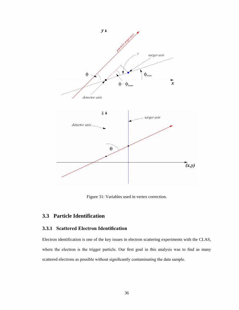
3.2.3 Vertex correction
Due to the offset of the beam position, which leads to an azimuthal angle () dependence of the Z
vertex reconstruction, a correction was made using simple geometrical considerations (see Fig.
31) in the form:
cos( )tan( )
corr rec beam
rZ Z
(19)
where Zcorr is the real vertex position along the target axis from where the detected electron has
originated, Zrec is the initial reconstructed uncorrected electron vertex, θ and υ are the polar and
the azimuthal electron scattering angles in the lab frame, and r is the distance from the axis along
the target to the actual beam line.
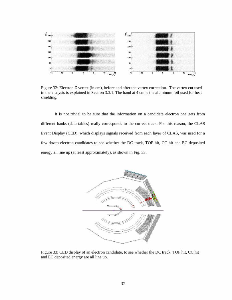
The beam offset, defined by beam and r was obtained from a fit to the distribution of the
average vertex position over all sectors. As can be seen in Fig. 32, the Z-vertex after the
correction does not have a phi dependency and an accurate, common cut (section 3.3.1) on the
vertex position for each sector can now be applied.
36
Figure 31: Variables used in vertex correction.
3.3 Particle Identification
3.3.1 Scattered Electron Identification
Electron identification is one of the key issues in electron scattering experiments with the CLAS,
where the electron is the trigger particle. Our first goal in this analysis was to find as many
scattered electrons as possible without significantly contaminating the data sample.
37
Figure 32: Electron Z-vertex (in cm), before and after the vertex correction. The vertex cut used
in the analysis is explained in Section 3.3.1. The band at 4 cm is the aluminum foil used for heat
shielding.
It is not trivial to be sure that the information on a candidate electron one gets from
different banks (data tables) really corresponds to the correct track. For this reason, the CLAS
Event Display (CED), which displays signals received from each layer of CLAS, was used for a
few dozen electron candidates to see whether the DC track, TOF hit, CC hit and EC deposited
energy all line up (at least approximately), as shown in Fig. 33.
Figure 33: CED display of an electron candidate, to see whether the DC track, TOF hit, CC hit
and EC deposited energy are all line up.

38
During data reconstruction, the software that is responsible for building final data events
(RECSIS/SEB, Simple Event Builder) assumes that only the very first particle in the data event
can be an electron and requires that the EC and SC hits are geometrically matched with a track
reconstructed in the drift chambers. It then assigns ID=11 and ID=0 to electron candidates that
pass and fail the requirements, respectively. Taking into consideration that SEB sometimes
mislabeled electrons as id=0 (i.e. as an unidentified negative track), we did not want to rely on the
SEB particle identification, and assumed that SEB ID=0 particle could be an electron if it fulfilled
the conditions below.
We also realized that, sometimes, the real electron has been detected and written out in a
later position in the event (about 1.4% of the electrons were recorded in secondary positions.)
These events were ignored in our analysis and an appropriate correction has been made.
Also noticed was a loss of electrons due to an error in the reconstruction code, which
passed incorrect information about the EC hit to the physics analysis. The error was that not all
the EC related banks (data tables) were properly filled. An empirical fix was implemented in the
analysis and the gain was found to be 14%.
Status Cut
The cut “status > 0” rejects tracks that pass the Hit Based Tracking (HBT) but fail the Time Best
Tracking (TBT) tests.
Z Vertex cut
With the vertex correction mentioned above, we were able to apply the same vertex cuts to
all six sectors. The cut was set from -3.5 to 3cm relative to the center of CLAS as is shown in Fig.
34. The same figure shows the target walls, as well as the entrance and exit foils. We decided to
use a wider cut assuming that there were not many deuteron events coming from the target walls.
39
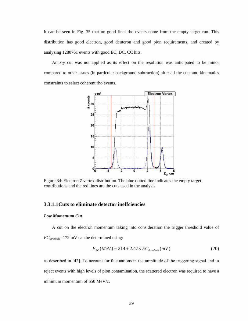
It can be seen in Fig. 35 that no good final rho events come from the empty target run. This
distribution has good electron, good deuteron and good pion requirements, and created by
analyzing 1280761 events with good EC, DC, CC hits.
An x-y cut was not applied as its effect on the resolution was anticipated to be minor
compared to other issues (in particular background subtraction) after all the cuts and kinematics
constraints to select coherent rho events.
Figure 34: Electron Z vertex distribution. The blue dotted line indicates the empty target
contributions and the red lines are the cuts used in the analysis.
3.3.1.1 Cuts to eliminate detector ineffciencies
Low Momentum Cut
A cut on the electron momentum taking into consideration the trigger threshold value of
ECthreshold=172 mV can be determined using:
( ) 214 2.47 ( )EC thresholdE MeV EC mV (20)
as described in [42]. To account for fluctuations in the amplitude of the triggering signal and to
reject events with high levels of pion contamination, the scattered electron was required to have a
minimum momentum of 650 MeV/c.

40
Figure 35: Two pion invariant mass distribution, showing that no good final rho (mass of 775
MeV and width of 150 MeV) events come from the empty target run (see Fig. 59 for
comparison).
Calorimeter Fiducial Cut
If an electron enters the EC too close (less than 10cm) to the detector edge, the resulting
electromagnetic shower is not fully contained within the detector volume and the deposited
energy is no longer related to the particle energy. Cuts are applied on the local coordinates of the
EC (U, V, and W) calculated from global coordinates X and Y to eliminate the electrons that are
incident near the edges of the detector.
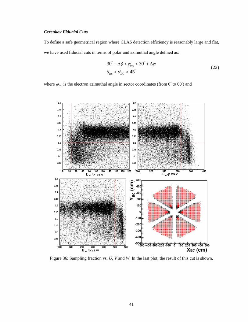
The cuts were developed by studying how the sampling fraction (the ratio of total energy
deposited in the calorimeter to momentum) varies with U, V and W as indicated in Fig. 36. The
design of the detector fixes the sampling fraction to 0.27. Near the edges of the detector this value
should decrease as the energy the electron deposited is not all collected due to shower leakage so
one can figure out which regions need to be discarded. The cuts selected (in cm units) were
EC EC ECU 25, V 365, and W 400 . (21)
41
Cerenkov Fiducial Cuts
To define a safe geometrical region where CLAS detection efficiency is reasonably large and flat,
we have used fiducial cuts in terms of polar and azimuthal angle defined as:
sec30 30
45cut DC
(22)
where sec is the electron azimuthal angle in sector coordinates (from 0◦ to 60
◦) and
Figure 36: Sampling fraction vs. U, V and W. In the last plot, the result of this cut is shown.
42
3375( )
sin( )
3375( )
cut
el
torus
epon
DC cut
C
el
torus
ED
p FI
A
epon B pI
(23)
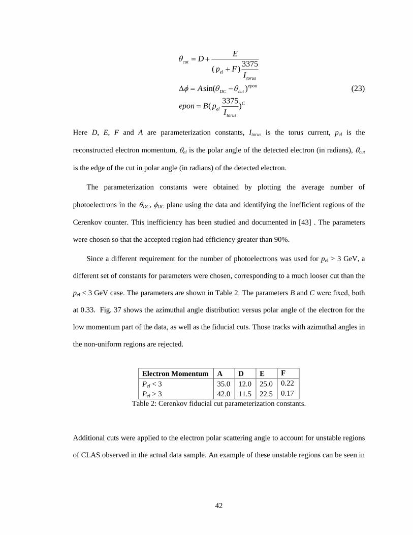
Here D, E, F and A are parameterization constants, Itorus is the torus current, pel is the
reconstructed electron momentum, el is the polar angle of the detected electron (in radians), cut
is the edge of the cut in polar angle (in radians) of the detected electron.
The parameterization constants were obtained by plotting the average number of
photoelectrons in the DC, DC plane using the data and identifying the inefficient regions of the
Cerenkov counter. This inefficiency has been studied and documented in [43] . The parameters
were chosen so that the accepted region had efficiency greater than 90%.
Since a different requirement for the number of photoelectrons was used for pel > 3 GeV, a
different set of constants for parameters were chosen, corresponding to a much looser cut than the
pel < 3 GeV case. The parameters are shown in Table 2. The parameters B and C were fixed, both
at 0.33. Fig. 37 shows the azimuthal angle distribution versus polar angle of the electron for the
low momentum part of the data, as well as the fiducial cuts. Those tracks with azimuthal angles in
the non-uniform regions are rejected.
Electron Momentum A D E F
Pel < 3 35.0 12.0 25.0 0.22
Pel > 3 42.0 11.5 22.5 0.17
Table 2: Cerenkov fiducial cut parameterization constants.
Additional cuts were applied to the electron polar scattering angle to account for unstable regions
of CLAS observed in the actual data sample. An example of these unstable regions can be seen in

43
Fig. 38 which shows the electron polar scattering angle as a function of electron momentum for
sector 5. These additional “holes” are due to bad TOF paddles or DC regions that malfunctioned
during the data taking.
Figure 37: Azimuthal angle distribution versus polar angle of the electron, for the low momentum
electrons. The applied fiducial cuts are shown in black solid lines. Those tracks with azimuthal
angles in the non-uniform regions are rejected.

44
The cuts have the form:
3375( )
3375( )
DC
el
torus
DC
el
torus
HG
p II
KJ
p LI
(24)
where the parameters G, H, I, J, K, L are listed in Table 3 .
Parameter sector 3 sector 5 sector 6
G 20.2 16.7 18.5
H 11 7 13
I 0.15 0.9 0.1
J 22.2 20.9 23
K 11 7 12
L 0.15 0.9 0.1
Table 3: Parameters to exclude angular regions for Sectors 3, 5 and 6.
Figure 38: Electron polar scattering angle vs momentum for sector 5. The “holes” due to bad
TOF paddles or DC regions that malfunctioned during the data taking are visible. They are
removed by the pel-θel cuts.

45
3.3.1.2 Cuts to eliminate π - misidentified as e
-
Cuts on energy deposition in the calorimeter
Electrons and pions can be distinguished in the calorimeter due to their different patterns of
energy deposition. Electrons emit photons and produce electromagnetic showers immediately
after they enter the calorimeter, with the total deposited energy proportional to their momentum
whereas pions are minimum ionizing particles (MIPs). We plot in Fig. 39 the total energy
deposited by the first particle in the calorimeter as a function of the energy deposited in the inner
layer of the calorimeter, both normalized to the total momentum of the particle. The
reconstruction code stores information about the deposited energy in the inner (ECin), outer
(ECout) and the whole (ECtot) electromagnetic calorimeters. Because ECin or ECout were frequently
absent, we took ECtot = max(ECout, ECin).
Figure 39: Total energy and inner energy deposited in the calorimeter, both normalized to the
momentum plotted as a function of electron momentum. The sharp edge at 3 GeV is the result of
using different fiducial cuts for below and beyond 3 GeV.
As expected, the plot shows a large signal that corresponds to electrons, and a small signal (pel ~
0.8 GeV) that corresponds to pions. We applied to following cuts:

46
/ 0.20 and / 0.08 if 3 Gev
/ 0.24 and / 0.06 if 3 Gev
tot el in el el
tot el in el el
EC p EC p p
EC p EC p p
(25)
Cuts on number of photoelectrons
An additional cut is provided by the Cerenkov detector, which has some efficiency for
distinguishing pions from electrons. A typical photoelectron distribution (number of
photoelectrons X 10) is shown in Fig. 40. Electrons are required to have a signal in the Cerenkov
detector, however some high energy pions that have sufficient velocity can also emit Cerenkov
light and produce a signal. The peak at ~2 photoelectrons corresponds to these pions and
Figure 40: Photoelectron distribution for different momentum bins. It is more difficult to
distinguish pions and electrons at momentum higher that 2.5 GeV.
47
need to be removed. The cuts are slightly different for low and high momentum particles. It is
more difficult to distinguish pions and electrons at momentum higher that 2.5 GeV as shown in
Fig. 40, but not many pions are expected at these kinematics, so the cuts are looser for the high
momentum particles.
nphe > 10 if 3 Gev
nphe < 25 if 3 Gev
el
el
p
p
(26)
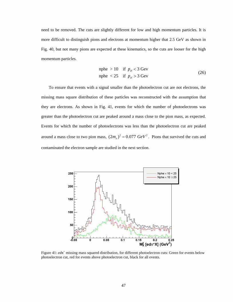
To ensure that events with a signal smaller than the photoelectron cut are not electrons, the
missing mass square distribution of these particles was reconstructed with the assumption that
they are electrons. As shown in Fig. 41, events for which the number of photoelectrons was
greater than the photoelectron cut are peaked around a mass close to the pion mass, as expected.
Events for which the number of photoelectrons was less than the photoelectron cut are peaked
around a mass close to two pion mass, 2 2(2 ) 0.077 m GeV . Pions that survived the cuts and
contaminated the electron sample are studied in the next section.
Figure 41: edπ+ missing mass squared distribution, for different photoelectron cuts: Green for events below
photoelectron cut, red for events above photoelectron cut, black for all events.
48
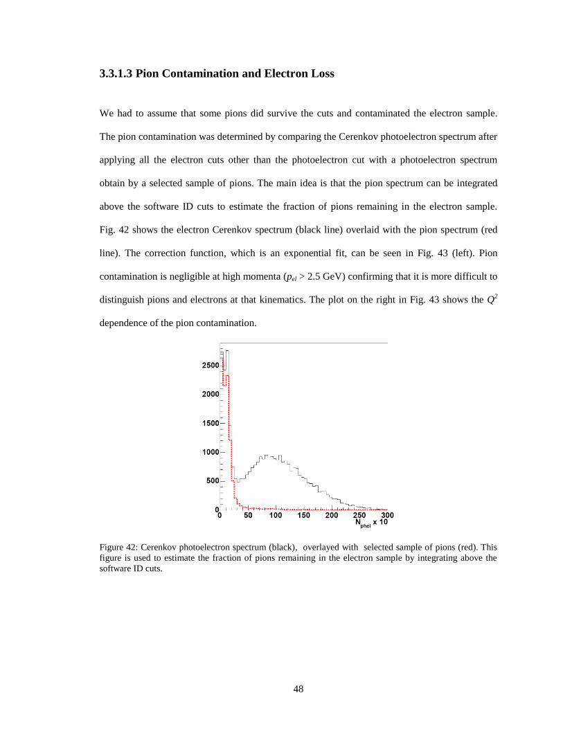
3.3.1.3 Pion Contamination and Electron Loss
We had to assume that some pions did survive the cuts and contaminated the electron sample.
The pion contamination was determined by comparing the Cerenkov photoelectron spectrum after
applying all the electron cuts other than the photoelectron cut with a photoelectron spectrum
obtain by a selected sample of pions. The main idea is that the pion spectrum can be integrated
above the software ID cuts to estimate the fraction of pions remaining in the electron sample.
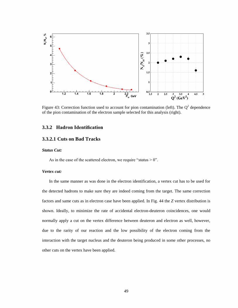
Fig. 42 shows the electron Cerenkov spectrum (black line) overlaid with the pion spectrum (red
line). The correction function, which is an exponential fit, can be seen in Fig. 43 (left). Pion
contamination is negligible at high momenta (pel > 2.5 GeV) confirming that it is more difficult to
distinguish pions and electrons at that kinematics. The plot on the right in Fig. 43 shows the Q2
dependence of the pion contamination.
Figure 42: Cerenkov photoelectron spectrum (black), overlayed with selected sample of pions (red). This
figure is used to estimate the fraction of pions remaining in the electron sample by integrating above the
software ID cuts.
49
Figure 43: Correction function used to account for pion contamination (left). The Q2 dependence
of the pion contamination of the electron sample selected for this analysis (right).
3.3.2 Hadron Identification
3.3.2.1 Cuts on Bad Tracks
Status Cut:
As in the case of the scattered electron, we require “status > 0”.
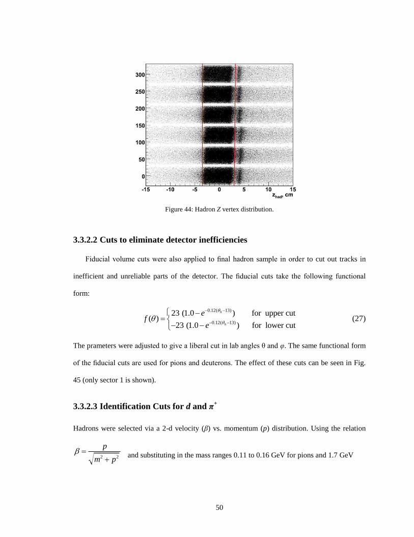
Vertex cut:
In the same manner as was done in the electron identification, a vertex cut has to be used for
the detected hadrons to make sure they are indeed coming from the target. The same correction
factors and same cuts as in electron case have been applied. In Fig. 44 the Z vertex distribution is
shown. Ideally, to minimize the rate of accidental electron-deuteron coincidences, one would
normally apply a cut on the vertex difference between deuteron and electron as well, however,
due to the rarity of our reaction and the low possibility of the electron coming from the
interaction with the target nucleus and the deuteron being produced in some other processes, no
other cuts on the vertex have been applied.
50
Figure 44: Hadron Z vertex distribution.
3.3.2.2 Cuts to eliminate detector inefficiencies
Fiducial volume cuts were also applied to final hadron sample in order to cut out tracks in
inefficient and unreliable parts of the detector. The fiducial cuts take the following functional
form:
0.12( 13)
0.12( 13)
23 (1.0 ) for upper cut( )
23 (1.0 ) for lower cut
h
h
ef
e
(27)
The prameters were adjusted to give a liberal cut in lab angles θ and υ. The same functional form
of the fiducial cuts are used for pions and deuterons. The effect of these cuts can be seen in Fig.
45 (only sector 1 is shown).
3.3.2.3 Identification Cuts for d and π+
Hadrons were selected via a 2-d velocity (β) vs. momentum (p) distribution. Using the relation
2 2
p
m p
and substituting in the mass ranges 0.11 to 0.16 GeV for pions and 1.7 GeV
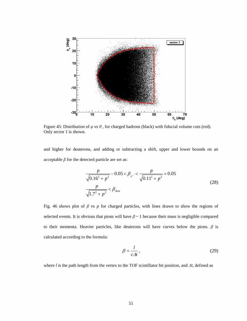
51
Figure 45: Distribution of υ vs θ , for charged hadrons (black) with fiducial volume cuts (red).
Only sector 1 is shown.
and higher for deuterons, and adding or subtracting a shift, upper and lower bounds on an
acceptable β for the detected particle are set as:
2 2 2 2
2 2
0.05 0.050.16 0.11
1.7deut
p p
p p
p
p
(28)
Fig. 46 shows plot of β vs p for charged particles, with lines drawn to show the regions of
selected events. It is obvious that pions will have β ~ 1 because their mass is negligible compared
to their momenta. Heavier particles, like deuterons will have curves below the pions. β is
calculated according to the formula:
l
c t
, (29)
where l is the path length from the vertex to the TOF scintillator hit position, and Δt, defined as
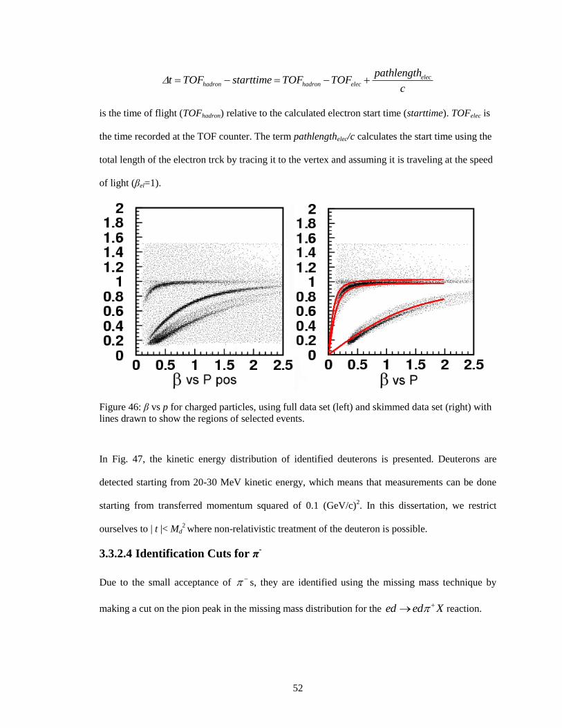
52
elechadron hadron elec
pathlengtht TOF starttime TOF TOF
c
is the time of flight (TOFhadron) relative to the calculated electron start time (starttime). TOFelec is
the time recorded at the TOF counter. The term pathlengthelec/c calculates the start time using the
total length of the electron trck by tracing it to the vertex and assuming it is traveling at the speed
of light (βel=1).
Figure 46: β vs p for charged particles, using full data set (left) and skimmed data set (right) with
lines drawn to show the regions of selected events.
In Fig. 47, the kinetic energy distribution of identified deuterons is presented. Deuterons are
detected starting from 20-30 MeV kinetic energy, which means that measurements can be done
starting from transferred momentum squared of 0.1 (GeV/c)2. In this dissertation, we restrict
ourselves to | t |< Md2 where non-relativistic treatment of the deuteron is possible.
3.3.2.4 Identification Cuts for π-
Due to the small acceptance of s, they are identified using the missing mass technique by
making a cut on the pion peak in the missing mass distribution for the ed ed X reaction.
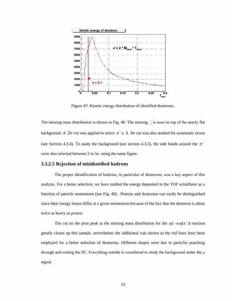
53
Figure 47: Kinetic energy distribution of identified deuterons.
The missing mass distribution is shown in Fig. 48. The missing is seen on top of the nearly flat
background. A 2 cut was applied to select s. A 3 cut was also studied for systematic errors
(see Section 4.3.4). To study the background (see section 4.3.3), the side bands around the
were also selected between 2 to 5σ using the same figure.
3.3.2.5 Rejection of misidentified hadrons
The proper identification of hadrons, in particular of deuterons, was a key aspect of this
analysis. For a better selection, we have studied the energy deposited in the TOF scintillator as a
function of particle momentum (see Fig. 49). Protons and deuterons can easily be distinguished
since their energy losses differ at a given momentum because of the fact that the deuteron is about
twice as heavy as proton.
The cut on the pion peak in the missing mass distribution for the ed ed X reaction
greatly cleans up this sample, nevertheless the additional cuts shown as the red lines have been
employed for a better selection of deuterons. Different shapes were due to particles punching
through and exiting the SC. Everything outside is considered to study the background under the ρ
signal.
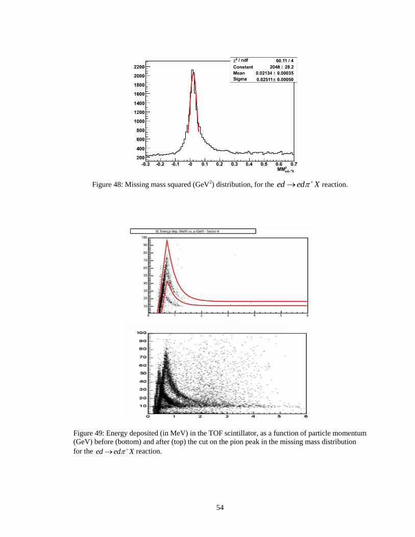
54
Figure 48: Missing mass squared (GeV2) distribution, for the ed ed X reaction.
Figure 49: Energy deposited (in MeV) in the TOF scintillator, as a function of particle momentum
(GeV) before (bottom) and after (top) the cut on the pion peak in the missing mass distribution
for the ed ed X reaction.
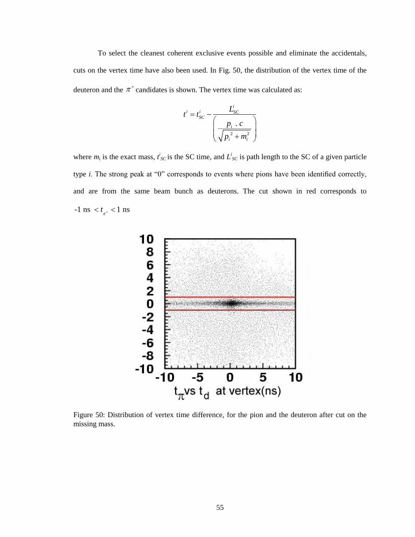
55
To select the cleanest coherent exclusive events possible and eliminate the accidentals,
cuts on the vertex time have also been used. In Fig. 50, the distribution of the vertex time of the
deuteron and the candidates is shown. The vertex time was calculated as:
2 2
.
ii i SC
SC
i
i i
Lt t
p c
p m
where mi is the exact mass, tiSC is the SC time, and L
iSC is path length to the SC of a given particle
type i. The strong peak at “0” corresponds to events where pions have been identified correctly,
and are from the same beam bunch as deuterons. The cut shown in red corresponds to
-1 ns 1 nst
Figure 50: Distribution of vertex time difference, for the pion and the deuteron after cut on the
missing mass.
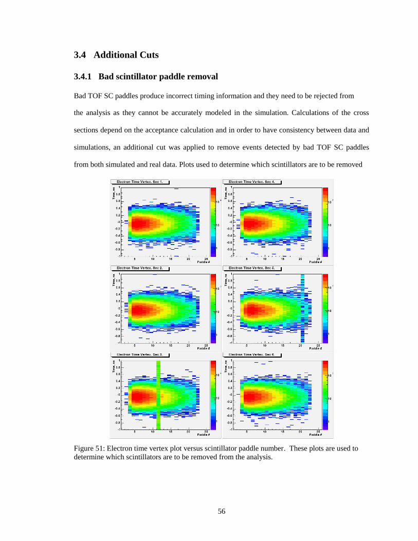
56
3.4 Additional Cuts
3.4.1 Bad scintillator paddle removal
Bad TOF SC paddles produce incorrect timing information and they need to be rejected from
the analysis as they cannot be accurately modeled in the simulation. Calculations of the cross
sections depend on the acceptance calculation and in order to have consistency between data and
simulations, an additional cut was applied to remove events detected by bad TOF SC paddles
from both simulated and real data. Plots used to determine which scintillators are to be removed
Figure 51: Electron time vertex plot versus scintillator paddle number. These plots are used to
determine which scintillators are to be removed from the analysis.
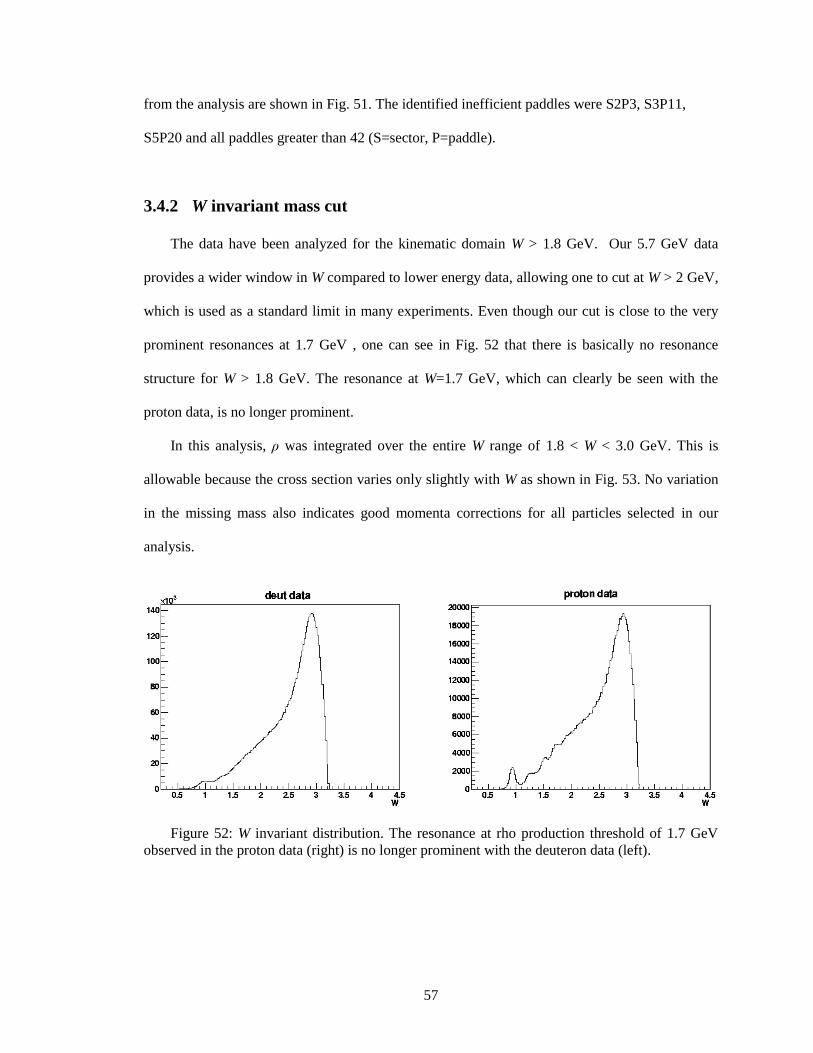
57
from the analysis are shown in Fig. 51. The identified inefficient paddles were S2P3, S3P11,
S5P20 and all paddles greater than 42 (S=sector, P=paddle).
3.4.2 W invariant mass cut
The data have been analyzed for the kinematic domain W > 1.8 GeV. Our 5.7 GeV data
provides a wider window in W compared to lower energy data, allowing one to cut at W > 2 GeV,
which is used as a standard limit in many experiments. Even though our cut is close to the very
prominent resonances at 1.7 GeV , one can see in Fig. 52 that there is basically no resonance
structure for W > 1.8 GeV. The resonance at W=1.7 GeV, which can clearly be seen with the
proton data, is no longer prominent.
In this analysis, ρ was integrated over the entire W range of 1.8 < W < 3.0 GeV. This is
allowable because the cross section varies only slightly with W as shown in Fig. 53. No variation
in the missing mass also indicates good momenta corrections for all particles selected in our
analysis.
Figure 52: W invariant distribution. The resonance at rho production threshold of 1.7 GeV
observed in the proton data (right) is no longer prominent with the deuteron data (left).
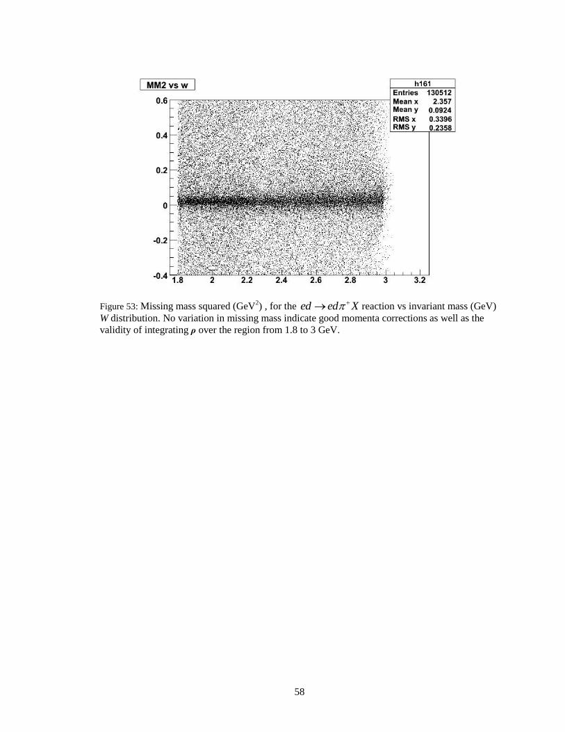
58
Figure 53: Missing mass squared (GeV2) , for the ed ed X reaction vs invariant mass (GeV)
W distribution. No variation in missing mass indicate good momenta corrections as well as the
validity of integrating ρ over the region from 1.8 to 3 GeV.
59
4 Yield Corrections, Extraction and Systematic Uncertainties
The main goal of this thesis is to measure the ratio of differential cross sections and this final
chapter is devoted to the description of how they have been extracted from the experimental data
and to the obtained results. As shown in Fig. 48, the missing mass of the detected d+ system
shows a missing - peak. After the selection of this
- peak, one can calculate the invariant mass
of +
-, which should show a typical rho mass distribution. We have chosen the invariant mass
technique over the missing mass technique as per the recommendation of [44]. The yields are
binned in some variables (Q2, t’, cosθh for fixed bins of 0.45<lc<0.55 fm and W > 1.8 GeV) and
corrected to obtain differential cross sections as described in section 1.4. The data correction
factors, followed by the process of extracting the yields from the +
- invariant mass
distribution, are presented next.
4.1 Data Correction Factors
4.1.1 Acceptance
Before extracting cross sections, acceptance corrections are applied on a bin-by-bin basis
according to
gen
w meas
MC
Nn n
N (30)
where nmeas is the measured yield, nw is the acceptance corrected yield, Ngen is the number of
events generated in the by the Monte Carlo (MC) simulation, and NMC are the number of events
that are “detected” within the simulation.
Events were generated based on the theoretical calculations of [10]. We slightly
improved the model by introducing new values for the b variable, which measures the size of the
interaction related to the side of the system composed by the target and the photon. In the old
model , the empirical values of 7 , 6, and 5 were used for Q2 < 1GeV
2, 1 GeV
2 < Q
2 < 2 GeV
2
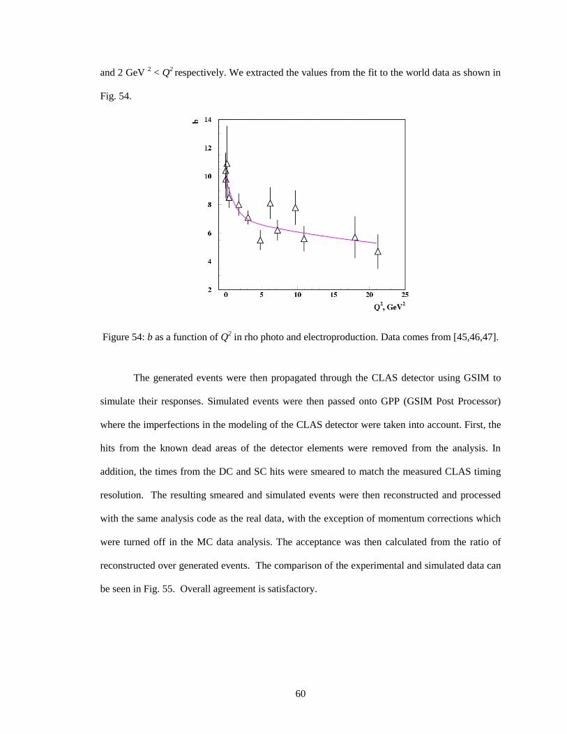
60
and 2 GeV 2 < Q
2 respectively. We extracted the values from the fit to the world data as shown in
Fig. 54.
Figure 54: b as a function of Q2 in rho photo and electroproduction. Data comes from [45,46,47].
The generated events were then propagated through the CLAS detector using GSIM to
simulate their responses. Simulated events were then passed onto GPP (GSIM Post Processor)
where the imperfections in the modeling of the CLAS detector were taken into account. First, the
hits from the known dead areas of the detector elements were removed from the analysis. In
addition, the times from the DC and SC hits were smeared to match the measured CLAS timing
resolution. The resulting smeared and simulated events were then reconstructed and processed
with the same analysis code as the real data, with the exception of momentum corrections which
were turned off in the MC data analysis. The acceptance was then calculated from the ratio of
reconstructed over generated events. The comparison of the experimental and simulated data can
be seen in Fig. 55. Overall agreement is satisfactory.
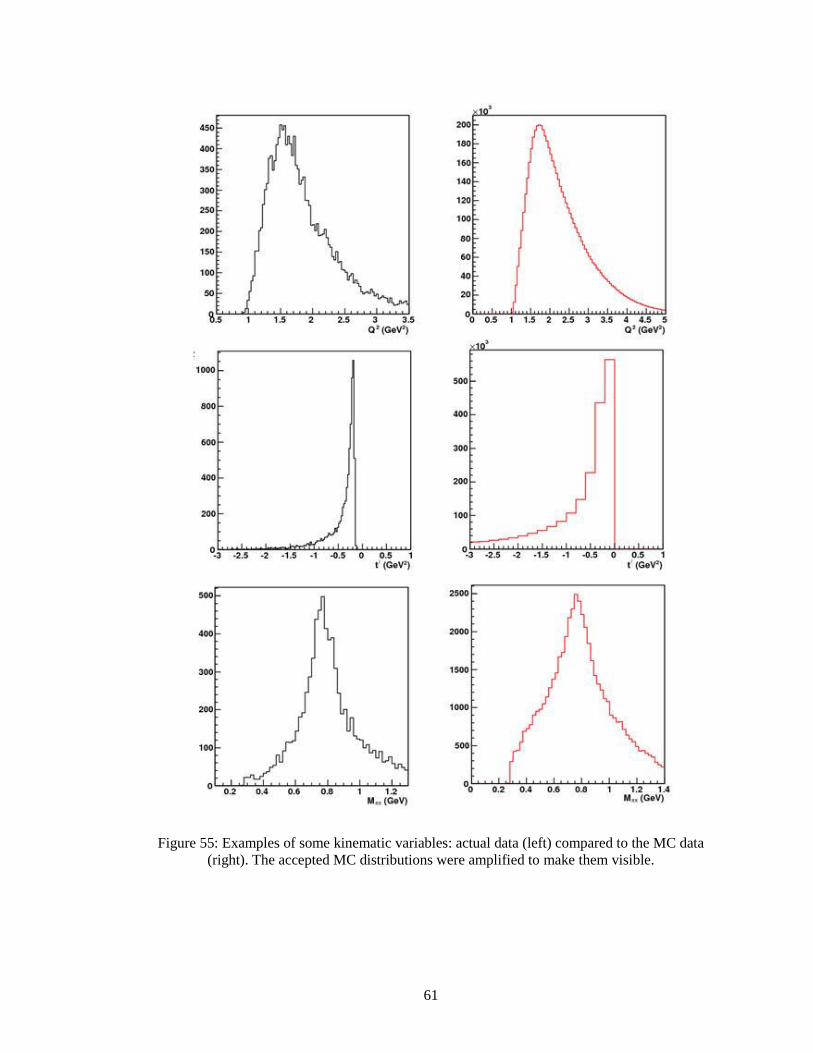
61
Figure 55: Examples of some kinematic variables: actual data (left) compared to the MC data
(right). The accepted MC distributions were amplified to make them visible.
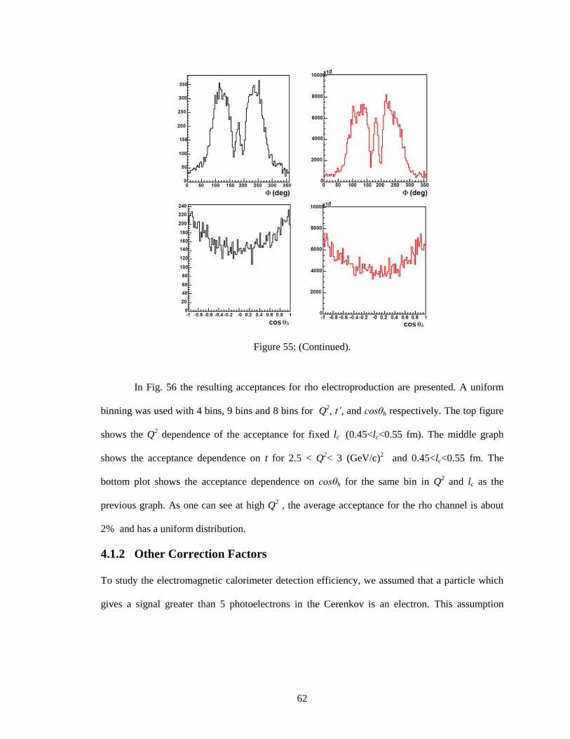
62
Figure 55: (Continued).
In Fig. 56 the resulting acceptances for rho electroproduction are presented. A uniform
binning was used with 4 bins, 9 bins and 8 bins for Q2, t’, and cosθh respectively. The top figure
shows the Q2 dependence of the acceptance for fixed lc (0.45<lc<0.55 fm). The middle graph
shows the acceptance dependence on t for 2.5 < Q2< 3 (GeV/c)
2 and 0.45<lc<0.55 fm. The
bottom plot shows the acceptance dependence on cosθh for the same bin in Q2 and lc as the
previous graph. As one can see at high Q2 , the average acceptance for the rho channel is about
2% and has a uniform distribution.
4.1.2 Other Correction Factors
To study the electromagnetic calorimeter detection efficiency, we assumed that a particle which
gives a signal greater than 5 photoelectrons in the Cerenkov is an electron. This assumption
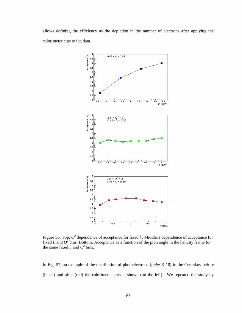
63
allows defining the efficiency as the depletion in the number of electrons after applying the
calorimeter cuts to the data.
Figure 56: Top: Q2 dependence of acceptance for fixed lc. Middle: t dependence of acceptance for
fixed lc and Q2 bins. Bottom: Acceptance as a function of the pion angle in the helicity frame for
the same fixed lc and Q2 bins.
In Fig. 57, an example of the distribution of photoelectrons (nphe X 10) in the Cerenkov before
(black) and after (red) the calorimeter cuts is shown (on the left). We repeated the study by
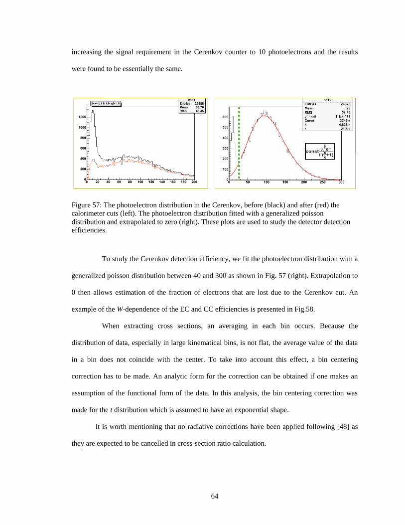
64
increasing the signal requirement in the Cerenkov counter to 10 photoelectrons and the results
were found to be essentially the same.
Figure 57: The photoelectron distribution in the Cerenkov, before (black) and after (red) the
calorimeter cuts (left). The photoelectron distribution fitted with a generalized poisson
distribution and extrapolated to zero (right). These plots are used to study the detector detection
efficiencies.
To study the Cerenkov detection efficiency, we fit the photoelectron distribution with a
generalized poisson distribution between 40 and 300 as shown in Fig. 57 (right). Extrapolation to
0 then allows estimation of the fraction of electrons that are lost due to the Cerenkov cut. An
example of the W-dependence of the EC and CC efficiencies is presented in Fig.58.
When extracting cross sections, an averaging in each bin occurs. Because the
distribution of data, especially in large kinematical bins, is not flat, the average value of the data
in a bin does not coincide with the center. To take into account this effect, a bin centering
correction has to be made. An analytic form for the correction can be obtained if one makes an
assumption of the functional form of the data. In this analysis, the bin centering correction was
made for the t distribution which is assumed to have an exponential shape.
It is worth mentioning that no radiative corrections have been applied following [48] as
they are expected to be cancelled in cross-section ratio calculation.
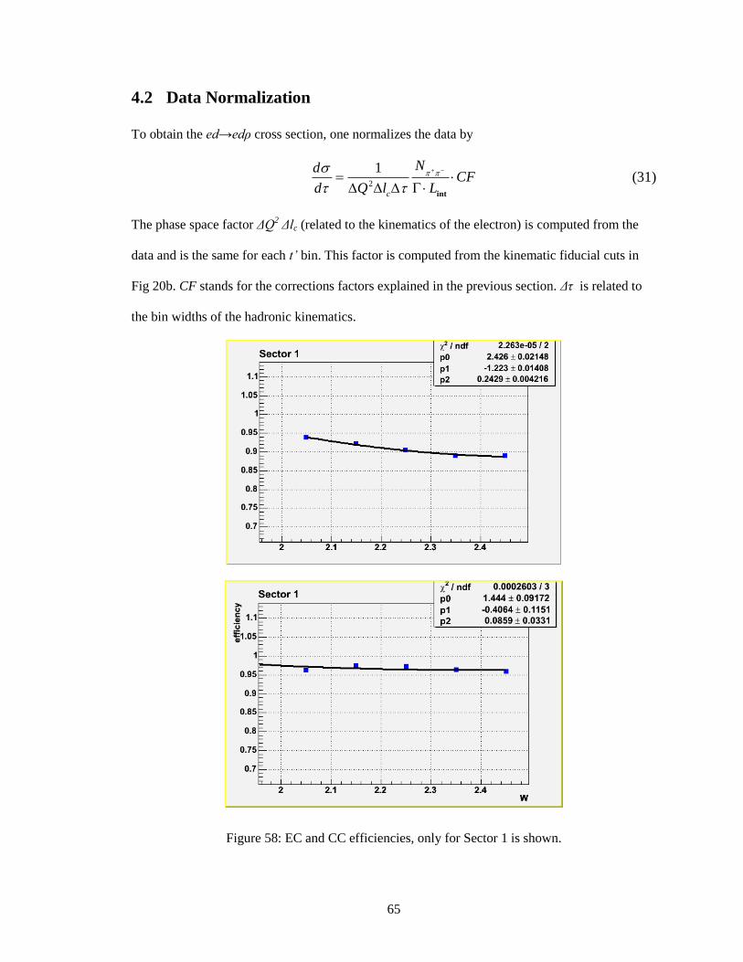
65
4.2 Data Normalization
To obtain the ed→edρ cross section, one normalizes the data by
2
1
c
NdCF
d Q l L
int
(31)
The phase space factor ΔQ2 Δlc (related to the kinematics of the electron) is computed from the
data and is the same for each t’ bin. This factor is computed from the kinematic fiducial cuts in
Fig 20b. CF stands for the corrections factors explained in the previous section. Δτ is related to
the bin widths of the hadronic kinematics.
Figure 58: EC and CC efficiencies, only for Sector 1 is shown.
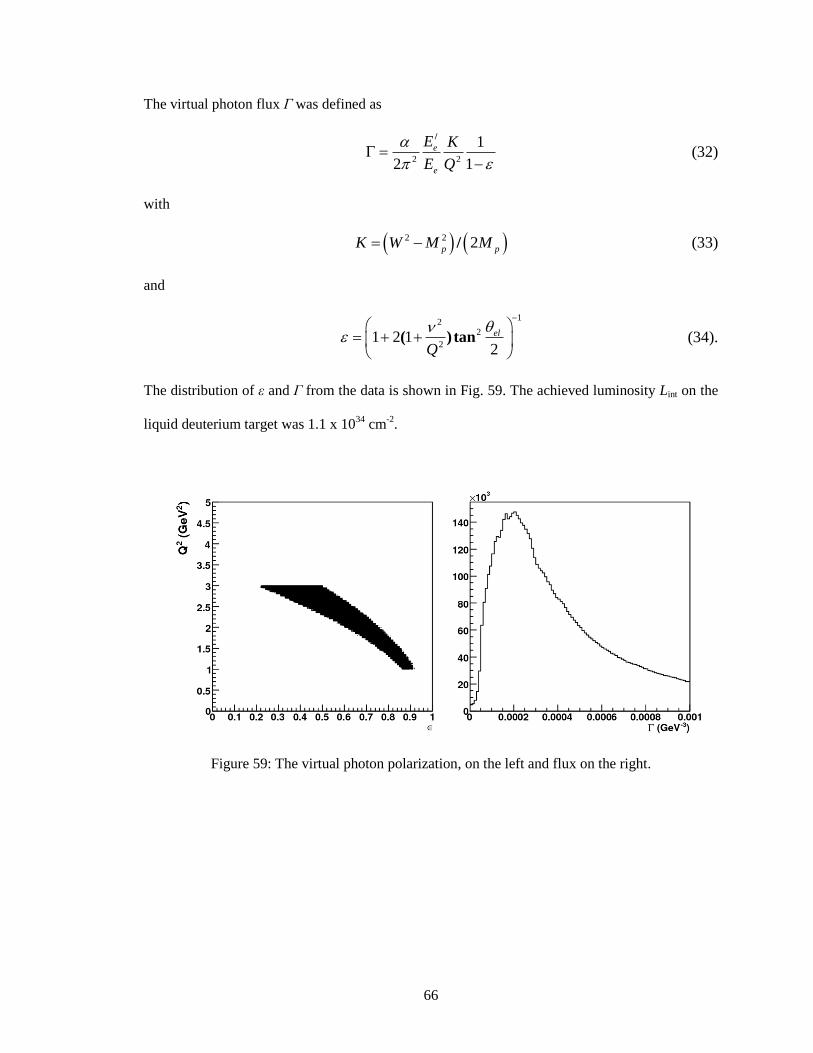
66
The virtual photon flux Г was defined as
2 2
1
2 1
e
e
E K
E Q
/
(32)
with
2 2 2p p
K W M M / (33)
and
12
2
21 2 1
2
el
Q
( ) tan (34).
The distribution of ε and Г from the data is shown in Fig. 59. The achieved luminosity Lint on the
liquid deuterium target was 1.1 x 1034
cm-2
.
Figure 59: The virtual photon polarization, on the left and flux on the right.
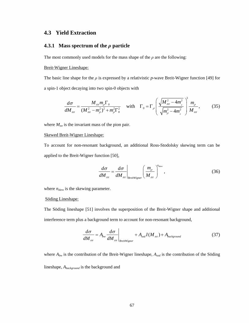
67
4.3 Yield Extraction
4.3.1 Mass spectrum of the ρ particle
The most commonly used models for the mass shape of the ρ are the following:
Breit-Wigner Lineshape:
The basic line shape for the ρ is expressed by a relativistic p-wave Breit-Wigner function [49] for
a spin-1 object decaying into two spin-0 objects with
32 2
0
02 2 2 2 2 2 20
4 with ,
( ) 4
M mM m md
dM M m m Mm m
(35)
where Mππ is the invariant mass of the pion pair.
Skewed Breit-Wigner Lineshape:
To account for non-resonant background, an additional Ross-Stodolsky skewing term can be
applied to the Breit-Wigner function [50],
,
skewn
BreitWigner
md d
dM dM M
(36)
where nskew is the skewing parameter.
Söding Lineshape:
The Söding lineshape [51] involves the superposition of the Breit-Wigner shape and additional
interference term plus a background term to account for non-resonant background,
( )bw sod background
BreitWigner
d dA A I M A
dM dM
(37)
where Abw is the contribution of the Breit-Wigner lineshape, Asod is the contribution of the Söding
lineshape, Abackground is the background and
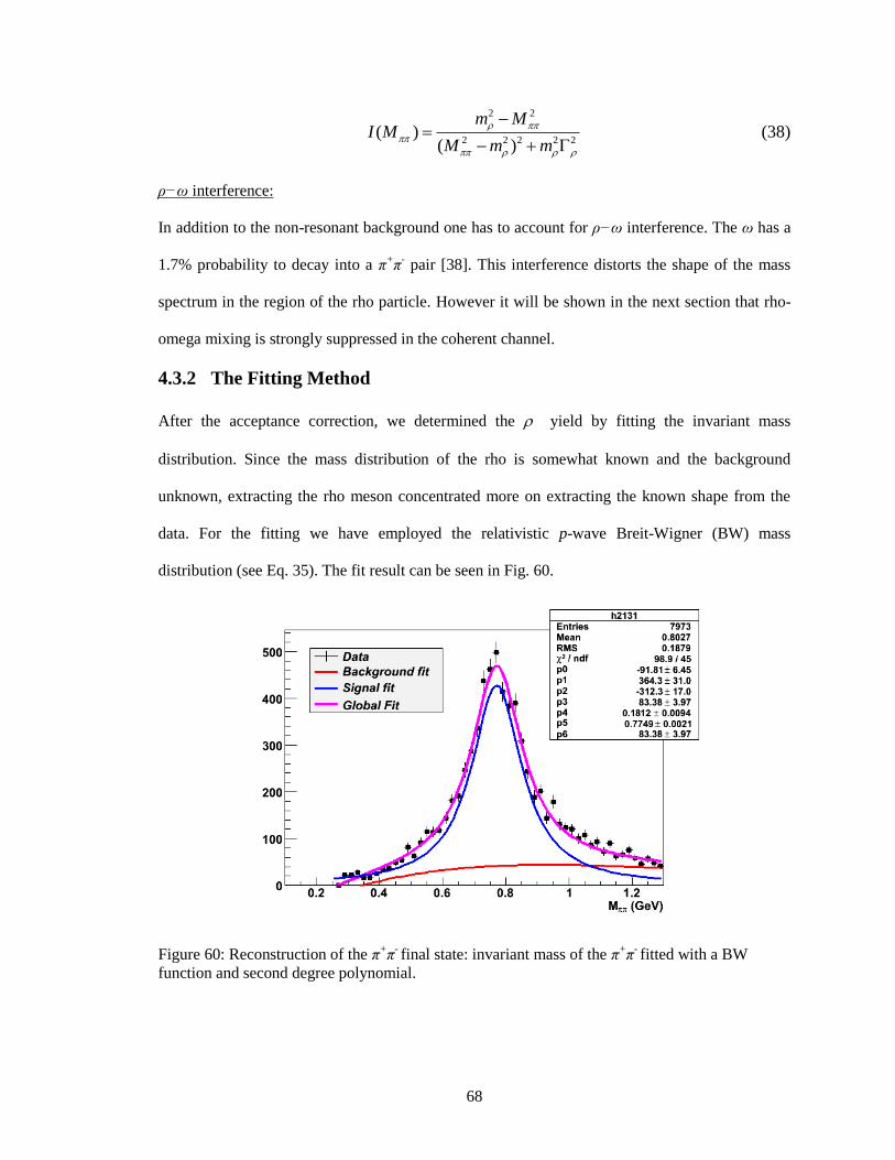
68
2 2
2 2 2 2 2( )
( )
m MI M
M m m
(38)
ρ−ω interference:
In addition to the non-resonant background one has to account for ρ−ω interference. The ω has a
1.7% probability to decay into a π+π
- pair [38]. This interference distorts the shape of the mass
spectrum in the region of the rho particle. However it will be shown in the next section that rho-
omega mixing is strongly suppressed in the coherent channel.
4.3.2 The Fitting Method
After the acceptance correction, we determined the yield by fitting the invariant mass
distribution. Since the mass distribution of the rho is somewhat known and the background
unknown, extracting the rho meson concentrated more on extracting the known shape from the
data. For the fitting we have employed the relativistic p-wave Breit-Wigner (BW) mass
distribution (see Eq. 35). The fit result can be seen in Fig. 60.
Figure 60: Reconstruction of the π+π
- final state: invariant mass of the π
+π
- fitted with a BW
function and second degree polynomial.
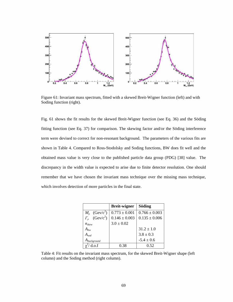
69
Figure 61: Invariant mass spectrum, fitted with a skewed Breit-Wigner function (left) and with
Soding function (right).
Fig. 61 shows the fit results for the skewed Breit-Wigner function (see Eq. 36) and the Söding
fitting function (see Eq. 37) for comparison. The skewing factor and/or the Söding interference
term were devised to correct for non-resonant background. The parameters of the various fits are
shown in Table 4. Compared to Ross-Stodolsky and Soding functions, BW does fit well and the
obtained mass value is very close to the published particle data group (PDG) [38] value. The
discrepancy in the width value is expected to arise due to finite detector resolution. One should
remember that we have chosen the invariant mass technique over the missing mass technique,
which involves detection of more particles in the final state.
Breit-wigner Söding
Mρ (Gev/c2) 0.773 ± 0.001 0.766 ± 0.003
Гρ (Gev/c2) 0.146 ± 0.003 0.135 ± 0.006
nskew 3.0 ± 0.02
Abw 31.2 ± 1.0
Asod 3.8 ± 0.3
Abackground -5.4 ± 0.6
χ2/ d.o.f 0.38 0.52
Table 4: Fit results on the invariant mass spectrum, for the skewed Breit-Wigner shape (left
column) and the Söding method (right column).
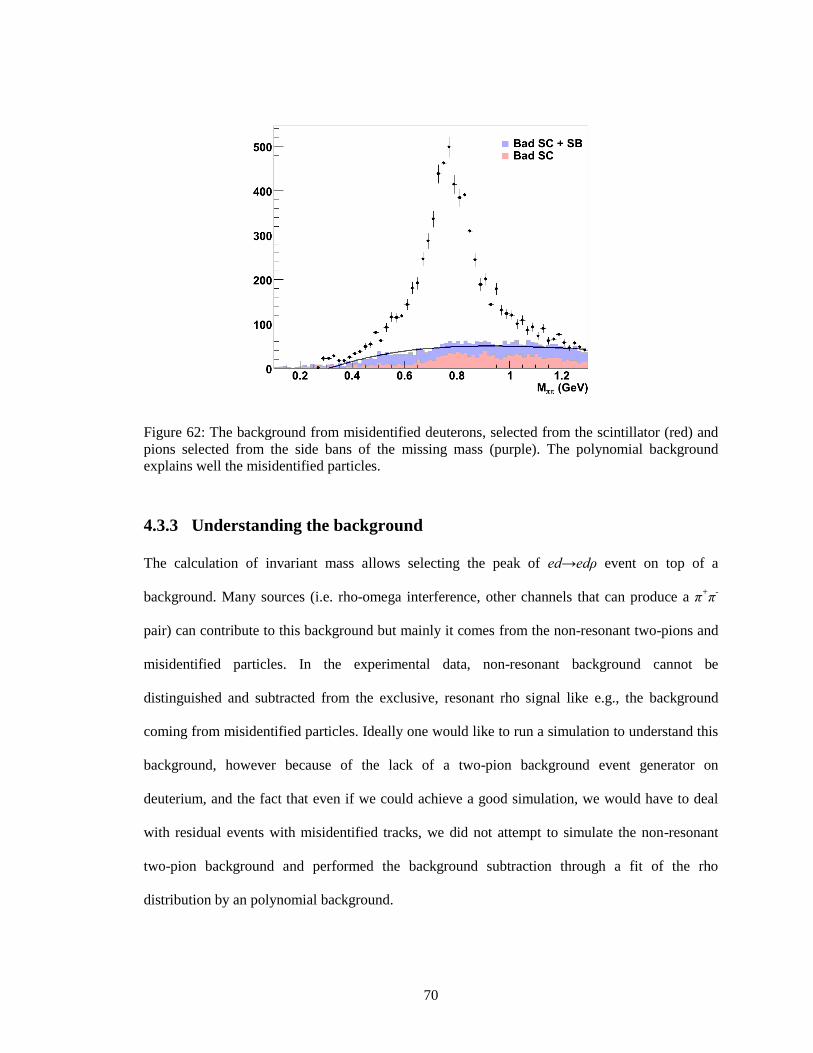
70
Figure 62: The background from misidentified deuterons, selected from the scintillator (red) and
pions selected from the side bans of the missing mass (purple). The polynomial background
explains well the misidentified particles.
4.3.3 Understanding the background
The calculation of invariant mass allows selecting the peak of ed→edρ event on top of a
background. Many sources (i.e. rho-omega interference, other channels that can produce a π+π
-
pair) can contribute to this background but mainly it comes from the non-resonant two-pions and
misidentified particles. In the experimental data, non-resonant background cannot be
distinguished and subtracted from the exclusive, resonant rho signal like e.g., the background
coming from misidentified particles. Ideally one would like to run a simulation to understand this
background, however because of the lack of a two-pion background event generator on
deuterium, and the fact that even if we could achieve a good simulation, we would have to deal
with residual events with misidentified tracks, we did not attempt to simulate the non-resonant
two-pion background and performed the background subtraction through a fit of the rho
distribution by an polynomial background.
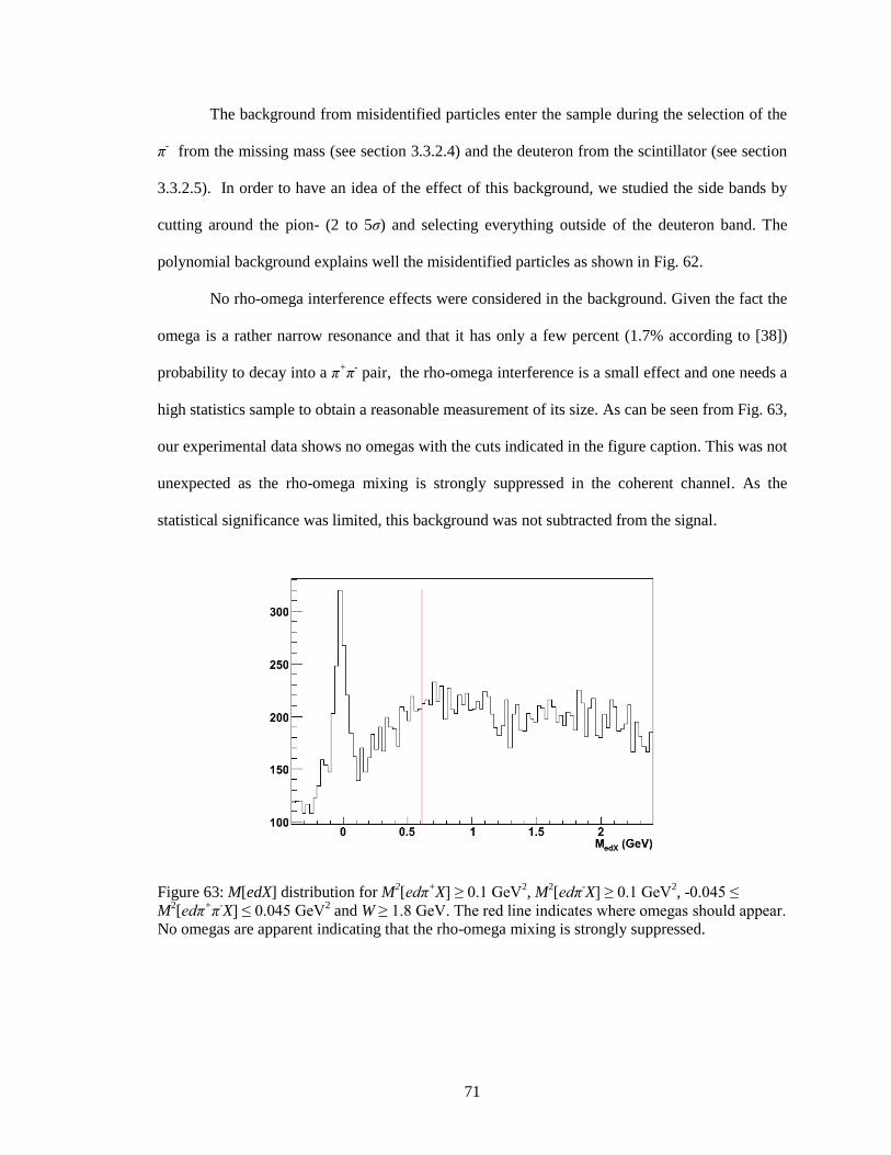
71
The background from misidentified particles enter the sample during the selection of the
π- from the missing mass (see section 3.3.2.4) and the deuteron from the scintillator (see section
3.3.2.5). In order to have an idea of the effect of this background, we studied the side bands by
cutting around the pion- (2 to 5σ) and selecting everything outside of the deuteron band. The
polynomial background explains well the misidentified particles as shown in Fig. 62.
No rho-omega interference effects were considered in the background. Given the fact the
omega is a rather narrow resonance and that it has only a few percent (1.7% according to [38])
probability to decay into a π+π
- pair, the rho-omega interference is a small effect and one needs a
high statistics sample to obtain a reasonable measurement of its size. As can be seen from Fig. 63,
our experimental data shows no omegas with the cuts indicated in the figure caption. This was not
unexpected as the rho-omega mixing is strongly suppressed in the coherent channel. As the
statistical significance was limited, this background was not subtracted from the signal.
Figure 63: M[edX] distribution for M2[edπ
+X] ≥ 0.1 GeV
2, M
2[edπ
-X] ≥ 0.1 GeV
2, -0.045 ≤
M2[edπ
+π
-X] ≤ 0.045 GeV
2 and W ≥ 1.8 GeV. The red line indicates where omegas should appear.
No omegas are apparent indicating that the rho-omega mixing is strongly suppressed.
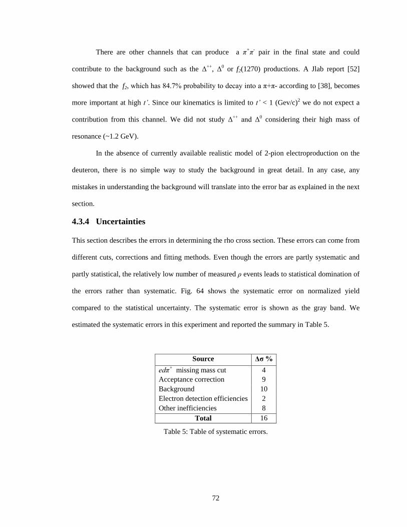
72
There are other channels that can produce a π+π
- pair in the final state and could
contribute to the background such as the Δ++
, Δ0 or f2(1270) productions. A Jlab report [52]
showed that the f2, which has 84.7% probability to decay into a π+π- according to [38], becomes
more important at high t’. Since our kinematics is limited to t’ < 1 (Gev/c)2 we do not expect a
contribution from this channel. We did not study Δ++
and Δ0 considering their high mass of
resonance (~1.2 GeV).
In the absence of currently available realistic model of 2-pion electroproduction on the
deuteron, there is no simple way to study the background in great detail. In any case, any
mistakes in understanding the background will translate into the error bar as explained in the next
section.
4.3.4 Uncertainties
This section describes the errors in determining the rho cross section. These errors can come from
different cuts, corrections and fitting methods. Even though the errors are partly systematic and
partly statistical, the relatively low number of measured ρ events leads to statistical domination of
the errors rather than systematic. Fig. 64 shows the systematic error on normalized yield
compared to the statistical uncertainty. The systematic error is shown as the gray band. We
estimated the systematic errors in this experiment and reported the summary in Table 5.
Source Δσ %
edπ+ missing mass cut 4
Acceptance correction 9
Background 10
Electron detection efficiencies 2
Other inefficiencies 8
Total 16
Table 5: Table of systematic errors.
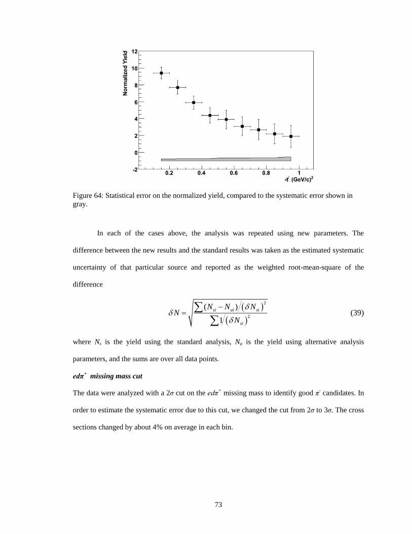
73
Figure 64: Statistical error on the normalized yield, compared to the systematic error shown in
gray.
In each of the cases above, the analysis was repeated using new parameters. The
difference between the new results and the standard results was taken as the estimated systematic
uncertainty of that particular source and reported as the weighted root-mean-square of the
difference
2
2
( )
1
si ai si
si
N N NN
N
(39)
where Ns is the yield using the standard analysis, Na is the yield using alternative analysis
parameters, and the sums are over all data points.
edπ+ missing mass cut
The data were analyzed with a 2σ cut on the edπ+ missing mass to identify good π
- candidates. In
order to estimate the systematic error due to this cut, we changed the cut from 2σ to 3σ. The cross
sections changed by about 4% on average in each bin.

74
Acceptance correction
The acceptance correction introduces a systematic error from a few, distinct sources. The first
comes from the model dependency. If the bins used to extract cross sections were infinitely small,
the acceptance calculation would have been model independent in principle. However because of
the finite bin width, our acceptances will differ slightly according to the event generator used. We
studied the model dependency by comparing our results to the ones generated by FSGEN [53], a
phase space event generator with a built in t-dependence for the t-channel meson production. This
yields a systematic error of 8%. The second source of systematic error associated with the
acceptance correction was estimated by combining bins, extracting the cross section in that bin
and comparing the result to the average of the cross sections from the constituent bins. This yields
a systematic error of 12.0%. The bin centering procedure also introduces a fairly small systematic
error (1%), mainly arising from small deviations of the data in each bin from polynomial form.
Background
The main source of systematic errors comes from the background subtraction. To derive the
error, we fitted the π+π
- invariant mass histogram with different functions and extracted different
rho numbers as shown in Fig. 65. For the final analysis, a BW and a second degree polynomial
has been employed and the difference between the number of ρ‟s obtained using these different
functions provided us the systematic error, which is found to be in the order of 10%.
Electron detection efficiencies
The determination of the CC efficiencies relies on the assumption that the distribution of signals
given by the electrons is a generalized Poisson function, and that the shape of this distribution
above 4 photoelectrons is sufficient to determine the whole distribution and to extrapolate to 0.
The maximum error we could make on the integral of the distribution between 0 and 4
photoelectrons is about 15%. Since the CC inefficiencies are at most of the order of 6%, the
corresponding systematic error on the cross sections is of 1%. The EC efficiency determination

75
relies on the assumption that a particle with nphe > 5 is a good scattered electron. We changed
this cut to 10 and the resulting difference was of the order of 2%.
Other inefficiencies
An additional systematic uncertainty of 8% was assigned to the whole data set to incorporate the
errors from other effects. This includes a 2% error to account for the estimated hardware trigger
inefficiency, 0.7% error to account for the loss of the electrons in the secondary positions in the
event data bank, possible unknown (not fully reproducible) detector and tracking inefficiencies,
minor variations in the target density, uncertainty in the FC charge measurement, etc.
Figure 65: Invariant Mass of π+π
- , fitted with different signal and background functions. The
functions are indicated at the top of each graph.
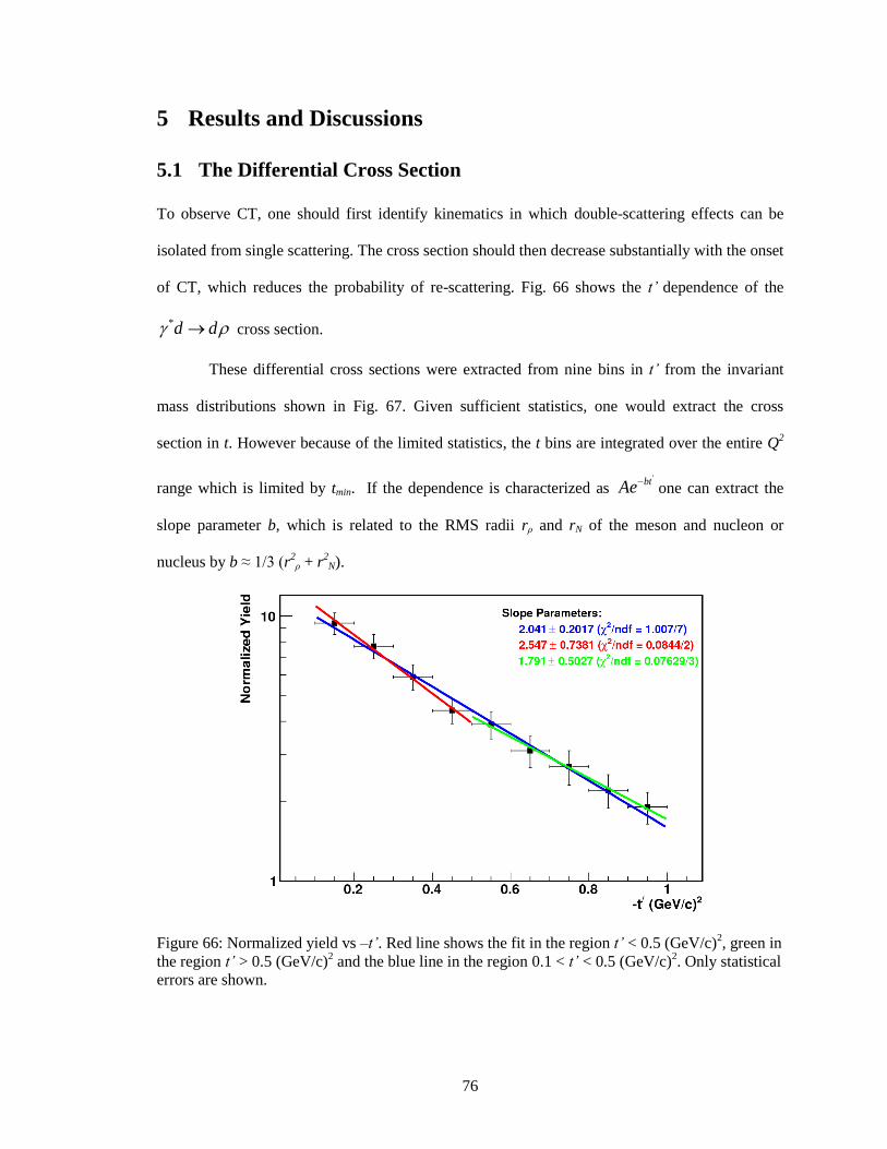
76
5 Results and Discussions
5.1 The Differential Cross Section
To observe CT, one should first identify kinematics in which double-scattering effects can be
isolated from single scattering. The cross section should then decrease substantially with the onset
of CT, which reduces the probability of re-scattering. Fig. 66 shows the t’ dependence of the
*d d cross section.
These differential cross sections were extracted from nine bins in t’ from the invariant
mass distributions shown in Fig. 67. Given sufficient statistics, one would extract the cross
section in t. However because of the limited statistics, the t bins are integrated over the entire Q2
range which is limited by tmin. If the dependence is characterized as 'btAeone can extract the
slope parameter b, which is related to the RMS radii rρ and rN of the meson and nucleon or
nucleus by b ≈ 1/3 (r2
ρ + r2N).
Figure 66: Normalized yield vs –t’. Red line shows the fit in the region t’ < 0.5 (GeV/c)2, green in
the region t’ > 0.5 (GeV/c)2 and the blue line in the region 0.1 < t’ < 0.5 (GeV/c)
2. Only statistical
errors are shown.
77
Figure 67: The invariant mass distributions, in nine bins used to extract the t/ dependence of the
*d d cross section.
The slope of the t’ distribution was obtained from the fit to the data in two regions (t’ <
0.5 (GeV/c)2 and t’ > 0.5 (GeV/c)
2). The slope parameters were 2.547 0.8532 (GeV/c)
2 (with
2/n= 0.0844/2) and 1.791 0.5027 (GeV/c)
2 (with
2/n= 0.07629/3) respectively. They are
indicated as red and green lines in Fig. 66. The slight change in the slope can be considered as a
possible indication of the re-scattering mechanism in rho final state. We also fit the data in the
range of 0.1 < t’ < 1.0 (GeV/c)2, one obtain a slope of 2.041 0.2017 (GeV/c)
2 (with
2/n=
1.007/7). The slope obtained from the full range of 0.1 < t’ < 1.0 (GeV/c)2
was in good
agreement with the one for production on the proton, as shown in Fig. 68.
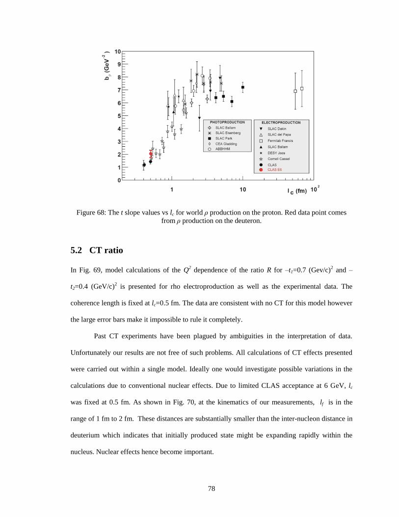
78
Figure 68: The t slope values vs lc for world ρ production on the proton. Red data point comes
from ρ production on the deuteron.
5.2 CT ratio
In Fig. 69, model calculations of the Q2 dependence of the ratio R for –t1=0.7 (Gev/c)
2 and –
t2=0.4 (GeV/c)2 is presented for rho electroproduction as well as the experimental data. The
coherence length is fixed at lc=0.5 fm. The data are consistent with no CT for this model however
the large error bars make it impossible to rule it completely.
Past CT experiments have been plagued by ambiguities in the interpretation of data.
Unfortunately our results are not free of such problems. All calculations of CT effects presented
were carried out within a single model. Ideally one would investigate possible variations in the
calculations due to conventional nuclear effects. Due to limited CLAS acceptance at 6 GeV, lc
was fixed at 0.5 fm. As shown in Fig. 70, at the kinematics of our measurements, lf is in the
range of 1 fm to 2 fm. These distances are substantially smaller than the inter-nucleon distance in
deuterium which indicates that initially produced state might be expanding rapidly within the
nucleus. Nuclear effects hence become important.

79
Figure 69: Cross section ratios at different momentum transfers and fixed lc , with different CT
assumptions: No CT (black), with two different CT predictions (upper and lower red). Only
statistical errors are shown.
Figure 70: lf vs lc distribution for the E6 data. For the kinematic used in our experiment, these
distances are substantially smaller than the inter-nucleon distance in deuterium.

80
A more accurate calculation with smaller error bars and a larger lc and lf coverage will be
possible when high statistics experiments on the deuteron becomes available after the CEBAF 12
GeV upgrade. While the predicted theoretical uncertainties are expected to shrink substantially
for the ratio of longitudinal cross sections, extracting this component requires s-channel helicity
conservation. The next section describes the steps taken to test the SCHC hypothesis.
5.3 Check of SCHC
Separating the longitudinal part of the rho cross section from the transverse part involves the
measurements of the total cross sections at different energies and performing a Rosenbluth
separation. In the case of the vector meson production, this separation can be done using the
meson decay angular distributions. Therefore by studying the decay pions we could identify the
polarization of the rho meson and the polarization of the virtual photon as helicity conservation
assumes that the two are equal. Experiments at Desy and Cornell have verified, using the angular
rho decay distribution, that the helicity is conserved at 90% level in the s-channel on the proton
data. There is no available data for rho electroproduction on the deuteron. The presented data are
the first data on this reaction.
In order to test the SCHC hypothesis, we fit the background subtracted azimuthal angle
( ) distribution with the function
04
1 1
11 2 2
2( ) [ cos( )]W r
(40)
to extract the parameter04
1 1r . SCHC assumes this parameter to be zero. Fig. 71 shows the dσ/dυπ
distribution for our data integrated over all kinematics. The purple line shows the fit using
equation 18, and the blue line shows a constant fit.

81
For the fit of equation 18, 04
1 1r = 0.042 0.02 (
2/n=6.9/7) while the constant fit gives
04
1 1r =
1.023 0.04642 with 2/n = 4.556/7 respectively. These fit results indicate a small but
statistically significant value for 04
1 1r , in contradiction to SCHC hypothesis. The fits to the
invariant mass distribution used the extract the phi distribution are shown in Fig. 72.
Figure 71: Phi distribution integrated over all kinematics. The purple and blue lines show
different fits. Only statistical errors are shown.
5.4 Ratio of longitudinal to tranverse cross section
While there is a slight indication that the SCHS hypothesis is violated, assuming that 04
1 1r is
negligible allows us to determine the parameter related to the ratio of longitudinal to transverse
cross section. We fit the cosθh distribution of the background subtracted data with the Eq. 18 to
extract 04
00r . In order to obtain the projection from the data, the π
+π
- invariant mass distribution is
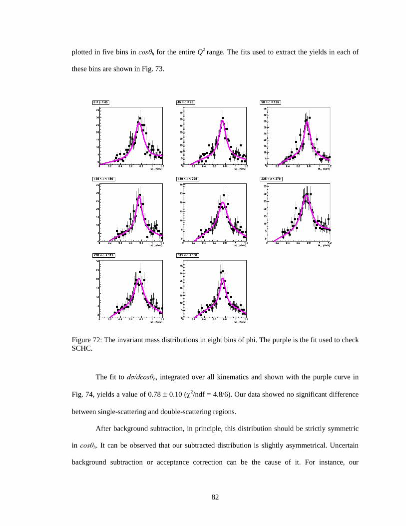
82
plotted in five bins in cosθh for the entire Q2
range. The fits used to extract the yields in each of
these bins are shown in Fig. 73.
Figure 72: The invariant mass distributions in eight bins of phi. The purple is the fit used to check
SCHC.
The fit to dσ/dcosθh, integrated over all kinematics and shown with the purple curve in
Fig. 74, yields a value of 0.78 0.10 (2/ndf = 4.8/6). Our data showed no significant difference
between single-scattering and double-scattering regions.
After background subtraction, in principle, this distribution should be strictly symmetric
in cosθh. It can be observed that our subtracted distribution is slightly asymmetrical. Uncertain
background subtraction or acceptance correction can be the cause of it. For instance, our
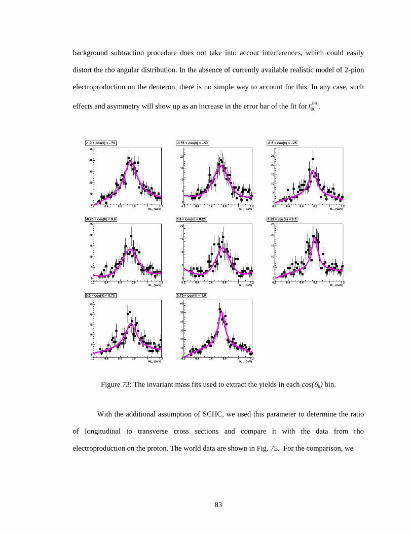
83
background subtraction procedure does not take into accout interferences, which could easily
distort the rho angular distribution. In the absence of currently available realistic model of 2-pion
electroproduction on the deuteron, there is no simple way to account for this. In any case, such
effects and asymmetry will show up as an increase in the error bar of the fit for04
00r .
Figure 73: The invariant mass fits used to extract the yields in each cos(h) bin.
With the additional assumption of SCHC, we used this parameter to determine the ratio
of longitudinal to transverse cross sections and compare it with the data from rho
electroproduction on the proton. The world data are shown in Fig. 75. For the comparison, we

84
computed using an average of Q2 and ε and used Eq. 19. Ideally one would like to extract values
for each Q2 bin and corresponding ε, however since the statistics of our channel are extremely
limited, we used an average of Q2 and ε. Our ratio of longitudinal to transverse cross sections
value of 5.8 2.2 is much higher than for the proton, which is less than 3. This would suggest a
modification of the spin structure the rho-meson electroproduction amplitudes in the deuteron.
Figure 74: Cosine projection, background subtracted and fitted. Only statistical errors are shown.
Figure 75: Ratio of longitudinal to transverse cross sections, as a function of Q2 for different
experiments using proton data.
85
5.5 Summary and Conclusions
Coherent rho electroproduction on the deuteron was studied using the CLAS E6 data in the range
of 1< Q2 < 3 (GeV/c)
2, 0.1 < t’ < 1.0 (GeV/c)
2 and < lc > fixed at 0.5 fm The following
conclusions were made using this data:
The differential cross sections for coherent rho electroproduction on the deuteron were
measured for the first time. A slight change in the t-slope dependence of the differential cross
section was observed which suggests a possible re-scattering mechanism in rho final state.
The ratio of two differential cross sections at the same Q2 and lc but at different t, the first
one in the double scattering region, and the second one in the single scattering region, was
measured. It was concluded that a significantly larger data set is necessary to distinguish whether
the CT effect is present or not.
The decay angular distributions were measured for the first time. The spin density matrix
elements 04
1 1r were extracted from the data. Evidence of the helicity non-conservation was found.
Assuming SCHC, the ratio of longitudinal to transverse cross section was extracted and
found to be significantly higher than for production on the proton.
86
REFERENCES
[1] S. J. Brodsky and A. H. Mueller, Phys. Lett. B 206, 685 (1988).
[2] A. H. Mueller, “ Proceedings of the Seventeenth Recontre de Moriond”, Conference on
Elementary Particle Physics, Les Arcs, France, 1982, edited by J. Tran Than Van (Editions
Frontieres, Gif-sur-Yvette, France,1982), p.13. : S. J. Brodsky, “ Proceedings of the Thirteenth
International Symposium on Multiparticle Dynamics”, Volendam, The Netherlands, 1982, edited
by W. Kittel et al. (World Scientific, Singapore, 1983), p. 963.
[3] D. H. Perkins, Phil. Mag. 46, 1146 (1955).
[4] R. J. Glauber, in: Lectures in theoretical physics, ed. W. E. Brittin et al. (Interscience
Publishers, New York, 1959), vol. I, p 315.
[5] J.C. Collins et al., Phys. Rev. D 56 2982 (1997).
[6] L.L. Frankfurt, G.A. Miller, and M.I. Strikman, Comments Nucl. Part. Phys. 21, 1(1992).
[7] A.S. Carroll et al., Phys. Rev. Lett. 61, 1698 (1988).
[8] B. Blattel et al., Phys. Rev. Lett. 70, 896 (1993).
[9] R.L. Anderson et al., Phys. Rev. D 4 3245 (1971).
[10] L. Frankfurt et al. , Nucl. Phys A, 622, 511-537 (1997); M. Sargsian, Computer code
(private communication).
[11] K. Schilling et al., Nucl. Phys. B61 381 (1973).
[12] Y. Mardor et al., Phys. Rev. Lett. 81, 5085 (1998).
[13] A. Leksanov et al., hepex/0101039 (2001).
[14] J.P. Ralston and B. Pire, Phys. Rev. Lett. 61, (1988), 1823; J.P. Ralston and B.Pire, Phys.
Rev. Lett. 65, (1990), 2343.
[15] S. J. Brodsky, and G. F. de Teramond,Phys. Rev. Lett. 60, 1924 (1988).
[16] N.C.R. Makins et al., Phys. Rev. Lett. 72, 1986 (1994); T.G. O'Neill et al., Phys.Lett. 351,
87 (1995).
[17] D. Abbott et al., Phys. Rev. Lett. 80, 5072 (1998).
[18] K. Garrow et al., Phys. Rev. C 66, 044613 (2002).
[19] V. R. Pandharipande and S. C. Pieper, Phys. Rev. C 45,(1992), 791; H. Gao, V. R.
Pandharipande and S. C. Pieper (private communication).
87
[20] E. M. Aitala et al., Phys. Rev. Lett. 86, (2001),4773.
[21] G. Bertsh, S.J. Brodsky, A.S. Goldhaber, J. Gunion, Phys. Rev. Lett. 47, 297 (1981).
[22] L.L. Frankfurt, G.A. Miller, and M. Strikman, Phys. Lett. B304, 1 (1993).
[23] L.L. Frankfurt, G.A. Miller, and M. Strikman, Found. of Phys. 30, 533 (2000).
[24] M.R. Adams et al., Phys. Rev. Lett. 74, 1525 (1995).
[25] K.Ackerstaff et al.,Phys. Rev. Lett.82, 3025 (1999).
[26] G. N. McClellan et al., Phys. Rev. Lett. 23, 554 (1969).
[27] J. Hüfner et al., Phys. Lett. B 383, 362 (1996); B. Z. Kopeliovich and J. Nemchik (private
communication).
[28] A. Airapetian et al., Phys. Rev. Lett. 90, (2003),052501.
[29] Dutta et al., Phys. Rev. C 68, 021001 (2003).
[30] B. Clasie et al., nucl-ex/ arXiv:0707.1481v1 (2007).
[31] A. Larson, G. A. Miller, and M. I. Strikman, Phys. Rev. C 74, 018201 (2006); A. Larson
(private communication).
[32] W. Cosyn, M. C. Martinez, J. Ryckebusch, and B. Van Overmeire, Phys. Rev. C 74,
062201(R) (2006); W. Cosyn and J. Ryckebusch (private communication).
[33] B. Mecking, et al., NIM A 503/3, 513 (2003)
[34] M.D. Mestayer et al., NIM A 449 (2000) 81
[35] E.S. Smith et al., NIM A 432 (1999) 265
[36] M. Amarian et al., NIM A 460, 239 (2001)
[37] G. Adams et al., NIM A 465, 414 (2001)
[38] W.-M.Yao et al. (Particle Data Group), J. Phys. G 33, 1 (2006) and 2007 partial update for
the 2008 edition.
[39] CLAS GEANT Simulation, http://www.physics.unh.edu/maurik/gsim_info.shtml
[40] A. Klimenko and S. Kuhn, Momentum Corrections for E6, CLAS-Notes 03-005; Jefferson
Laboratory
[41] S. Stepanyan, Beam energy measurement with ep ep elastic scattering on CLAS, CLAS-
Notes 02-008; Jefferson Laboratory

88
[42] K.S. Egiyan, Determination of Electron Energy cut due to the CLAS EC Threshold, CLAS-
Notes 99-007, Jefferson Laboratory
[43] CLAS Cerenkov detector, http://www.jlab.org/~vlassov/cc/index.html
[44] C.A. Meyer, M. Willaims and R. Bradford, Computing Invariant Masses and Missing
Masses, CLAS-Notes 04-008; ; Jefferson Laboratory
[45] C. Adloff et al., Eur. Phys. J. C13 (2000) 371.
[46] J. Breitweg et al., Eur. Phys. J. C6 (1999) 603.
[47] S. Aid et al., Nucl. Phys. B463 (1996) 3.
[48] I. Akushevich, Eur Phy Journal C, Volume 8, Issue 3, pp. 457-463 (1999).
[49] J.D. Jackson, II Nuovo Cimento 34 (1964), 1644; W.D. Shambroom et al., Phys. Rev. D 26,
(1982), 1.
[50] M.Ross and L. Stodolsky, Phys. Rev. 149, (1966), 1172.
[51] P. Söding, Phys. Lett. 19, (1966), 702.
[52] M. Battaglieri, CLAS-Analysis 2001-002 (2001).
[53] S. Stepanyan, Computer code (private communication).
89
VITA
ATILLA GÖNENÇ
EDUCATION
2002-2009 Ph.D. Candidate (Physics), Florida International University
1993-1997 B.Sc. (Physics), University of Ankara, Ankara, Turkey
WORK EXPERIENCE
2002-2006 Research/Teaching Assistant, Physics Department, Florida
International University
SELECTED PUBLICATIONS
Deeply virtual Compton scattering beam-spin asymmetries.
By CLAS Collaboration (F.X. Girod et al.). IRFU-08-24, JLAB-PHY-07-767, Nov 2007. 6pp.
Published in Phys.Rev.Lett.100:162002,2008.
Measurement of e p --> e p pi0 beam spin asymmetries above the resonance region.
By CLAS Collaboration (R. De Masi et al.). IRFU-08-23, JLAB-PHY-07-749, Nov 2007. 5pp.
Published in Phys.Rev.C77:042201,2008.
Cross sections and beam asymmetries for vec(e) p ---> en pi+ in the nucleon resonance region for
1.7 <= Q**2 <= 4.5-(GeV)**2.
By CLAS Collaboration (K. Park et al.). JLAB-PHY-07-720, Sep 2007. 23pp.
Published in Phys.Rev.C77:015208,2008.
First measurement of coherent phi-meson photoproduction on deuteron at low energies.
By CLAS Collaboration (T. Mibe et al.). JLAB-PHY-07-626, Mar 2007. 6pp.
Published in Phys.Rev.C76:052202,2007.
Cascade production in the reactions gamma p ---> K+ K+ (X) and gamma p ---> K+ K+ pi- (X).
L. Guo et al. JLAB-PHY-07-621, Feb 2007. 9pp.
Published in Phys.Rev.C76:025208,2007.