flow induced by a randomly vibrating boundary - arxiv · flow induced by a randomly vibrating...

arX

iv:n

lin/0

0010

50v1

[nl

in.P

S] 2

4 Ja

n 20

00

Under consideration for publication in J. Fluid Mech. 1

Flow induced by a randomly vibratingboundary

By DMITRI VOLFSON1 AND JORGE VINALS1,2

1Supercomputer Computations Research Institute, Florida State University, Tallahassee,Florida 32306-4130, USA

2 Department of Chemical Engineering, FAMU-FSU College of Engineering, Tallahassee,Florida 31310-6046, USA

(Received 12 June 2018)

We study the flow induced by random vibration of a solid boundary in an otherwisequiescent fluid. The analysis is motivated by experiments conducted under the low leveland random effective acceleration field that is typical of a microgravity environment.When the boundary is planar and is being vibrated along its own plane, the varianceof the velocity field decays as a power law of distance away from the boundary. If alow frequency cut-off is introduced in the power spectrum of the boundary velocity, thevariance decays exponentially for distances larger than a Stokes layer thickness based onthe cut-off frequency. Vibration of a gently curved boundary results in steady streamingin the ensemble average of the tangential velocity. Its amplitude diverges logarithmicallywith distance away from the boundary, but asymptotes to a constant value instead ifa low frequency cut-off is considered. This steady component of the velocity is shownto depend logarithmically on the cut-off frequency. Finally, we consider the case of aperiodically modulated solid boundary that is being randomly vibrated. We find steadystreaming in the ensemble average of the first order velocity, with flow extending up to acharacteristic distance of the order of the boundary wavelength. The structure of the flowin the vicinity of the boundary depends strongly on the correlation time of the boundaryvelocity.

1. Introduction

This paper examines the formation and separation of viscous layers in a fluid whichis in contact with a solid boundary that is vibrated randomly. The analysis is motivatedby the low level and random acceleration field that affects a number of microgravityexperiments. We first study the case of a planar boundary to generalize the classicalresult of Stokes (1851) who considered a boundary vibrated periodically along its ownplane. We next consider a slightly curved boundary, and show that steady streamingappears in the ensemble average at first order in the perturbed flow variables. Thereare several qualitative similarities and differences with the classical result by Schlichting(1979) for the case of periodic vibration. Finally, we address the case of a modulatedboundary that is vibrated randomly.Our study is motivated by the significant levels of residual accelerations (g-jitter) that

have been detected during space missions in which microgravity experiments have beenconducted (Walter (1987), Nelson (1991), DeLombard et al. (1997)). Direct measurementof these residual accelerations has shown that they have a wide frequency spectrum,ranging approximately from 10−4Hz to 102Hz. Amplitudes range from 10−6gE at the

http://arxiv.org/abs/nlin/0001050v1

2 D. Volfson and J. Vinals

lowest end of the frequency spectrum, and increase roughly linearly for high frequencies,reaching values of 10−4gE − 10−3gE at frequencies of around 10Hz (gE is the intensityof the gravitational field on the Earth’s surface). Despite the efforts of a number ofresearchers over the last decade, there remain areas of uncertainty about the potentialeffect of such a residual acceleration field on typical microgravity fluid experiments,especially in quantitative terms. A better understanding of the response of a fluid to suchdisturbances would enable improved experiment design to minimize or compensate fortheir influence. In addition, it would also be useful to have error estimates of quantitiesmeasured in the presence of residual accelerations, including whenever possible somemethodology for extrapolation to ideal zero gravity.The formation of viscous layers around solid boundaries when the flow amplitude

has a random component has not been addressed yet despite its potential relevancefor a number of microgravity experiments. Among them we mention the dynamics ofcolloidal suspensions, coarsening studies of solid-liquid mixtures in which purely diffusivecontrolled transport is desired, or the interaction between the viscous layer producedby bulk flow of random amplitude and the morphological instability of a crystal-meltinterface. Our study represents the first step in this direction, and focuses on simplegeometries in order to elucidate those salient features of the flow that arise from therandom nature of the vibration.Previous theoretical work on the influence of g-jitter on fluid flow ranges from order

of magnitude estimates to detailed numerical calculations. For example, the order ofmagnitude of the contributions to fluid flow from the residual acceleration field may beestimated from the length and time scales of a particular experiment, and the values of therelevant set of dimensionless numbers (Alexander (1990)). Such studies are of interest asa first approximation, but are not very accurate. Other studies have modeled the residualacceleration field by some simple analytic function in which the acceleration is typicallydecomposed into steady and time dependent components, the latter being periodic intime (Gershuni & Zhukhovitskii (1976), Kamotani et al. (1981), Alexander et al. (1991),Farooq & Homsy (1994), Grassia & Homsy (1998a), Grassia & Homsy (1998b), Gershuni& Lyubimov (1998)). A few studies have also addressed the consequences of isolatedpulses of short duration (Alexander et al. (1997)).Zhang et al. (1993) and Thomson et al. (1997) adopted a statistical description of the

residual acceleration field onboard spacecraft, and modeled the acceleration time seriesas a stochastic process in time. The main premise of this approach is that a statisticaldescription is necessary in those cases in which the characteristic time scales of the phys-ical process under investigation are long compared with the correlation time of g-jitter,τ (the acceleration amplitudes and orientations at two different times are statistically in-dependent if separated by an interval larger than τ). Progress has been achieved throughthe consideration of a specific stochastic model according to which each Cartesian com-ponent of the residual acceleration field ~g(t) is modeled as a narrow band noise. Thisnoise is a Gaussian process defined by three independent parameters: its intensity

⟨

g2⟩

,a dominant angular frequency Ω, and a characteristic spectral width τ−1. Each realiza-tion of narrow band noise can be viewed as a temporal sequence of periodic functionsof angular frequency Ω with amplitude and phase that remain constant only for a fi-nite amount of time (τ on average). At random intervals, new values of the amplitudeand phase are drawn from prescribed distributions. This model is based on the followingmechanism underlying the residual acceleration field: one particular natural frequencyof vibration of the spacecraft structure (Ω) is excited by some mechanical disturbanceinside the spacecraft, the excitation being of random amplitude and taking place at asequence of unknown (and essentially random) instants of time.

Flow induced by a randomly ... 3

Narrow band noise has been shown to describe reasonably well many of the featuresof g-jitter time series measured onboard Space Shuttle by Thomson et al. (1997). Actualg-jitter data collected during the SL-J mission were analyzed, and a time series of roughlysix hours was studied in detail. A scaling analysis revealed the existence of both deter-ministic and stochastic components in the time series. The deterministic contribution

appeared at a frequency of 17 Hz, with an amplitude⟨

g2⟩1/2

= 3.56× 10−4gE . Stochas-tic components included two well defined spectral features with a finite correlation time;

one at 22 Hz with⟨

g2⟩1/2

= 3.06 × 10−4gE and τ = 1.09 s, and one at 44 Hz with⟨

g2⟩1/2

= 5.20× 10−4gE and τ = 0.91 s. White noise background is also present in theseries with an intensity D = 8.61× 10−4cm2/s3.

A further theoretical advantage of narrow band noise is that it provides a convenientway of interpolating between monochromatic noise (akin to studies involving a determin-istic and periodic gravitational field), and white noise (in which no frequency componentis preferred). In the limit τ → 0 with D =

⟨

g2⟩

τ finite, narrow band noise reduces to

white noise of intensity D; whereas, for τ → ∞ with⟨

g2⟩

finite, monochromatic noise isrecovered.

We discuss in this paper the flow induced in an otherwise quiescent fluid by the randomvibration of a solid boundary. The velocity of the boundary u0(t) is assumed prescribed,and modeled as a narrow band stochastic process. First, we consider an infinite planarboundary that is being vibrated along its own plane to generalize the classical problemstudied by Stokes (1851). In the monochromatic limit, the variance of the velocity fielddecays exponentially away from the wall, with a characteristic decay length given by theStokes layer thickness δs = (2ν/Ω)1/2, where ν is the kinematic viscosity of the fluid,and Ω is the angular frequency of vibration of the boundary. Since the equations gov-erning the flow are linear, we are able to obtain an analytic solution describing transientlayer formation in the stochastic case, but only in the neighborhood of the white andmonochromatic noise limits. We then show that for any finite correlation time the sta-tionary variance of the tangential velocity asymptotically decays as the inverse squareddistance from the wall, in contrast with the exponential decay in the deterministic case.This asymptotic behavior originates from the low frequency range of the power spectrumof the boundary velocity. The crossover from power law to exponential decay is explicitlycomputed by introducing a low frequency cut-off in the power spectrum.

We next investigate two additional geometries in which the equations governing fluidflow are not linear, and show that several of the generic features obtained for the case ofa planar boundary still hold. In the first case, we generalize the analysis of Schlichting(1979) concerning secondary steady streaming. He found that the oscillatory motion ofthe boundary induces a steady secondary flow outside of the viscous boundary layer evenwhen the velocity of the boundary averages to zero. If the thickness of the Stokes layer,δs, and the amplitude of oscillation, a, are small compared with a characteristic lengthscale of the boundary L (δs ≪ L, a ≪ L), then the generation of secondary steadystreaming may be described as follows. Vibration of the rigid boundary gives rise to anoscillatory and nonuniform motion of the fluid. The flow is potential in the bulk, androtational in the boundary layer because of no-slip conditions on the boundary. The bulkflow applies pressure at the outer edge of boundary layer, which does not vary acrossthe layer. The non uniformity of the flow leads to vorticity convection in the boundarylayer through nonlinear terms. Both convection and the applied pressure drive vorticitydiffusion, and thus induce secondary steady motion which does not vanish outside of theboundary layer. In the simplest case in which the far field velocity is a standing wave


U(x, t) = U(x)cos(Ωt), the tangential component of the secondary steady velocity is,

u(s) = −3

4ΩUdU

dx, (1.1)

where x is a curvilinear coordinate along the boundary. In fact, Eq. (1.1) serves as theboundary condition for the stationary part of the flow in the bulk. Similar conclusionshave been later reached by Batchelor (1967) who studied sinusoidal oscillations of nonuni-form phase, and by Gershuni & Lyubimov (1998) who studied monochromatic oscillationsof a general form.The second geometry that we address is the so called wavy wall (Lyne (1971)). The

deterministic limit in which a wavy boundary is being periodically vibrated has beenstudied by a number of authors, mainly to address the interaction between the flow abovethe sea bed and ripple patterns on it (Lyne (1971), Kaneko & Honjii (1979), Vittori(1989), Blondeaux & Vittori (1994) and references therein). Lyne (1971) deduced theexistence of steady streaming in the limit in which the amplitude of the wall deviationfrom planarity is small compared with the thickness of the Stokes layer. He introduceda conformal transformation and obtained an explicit solution in the limit of small kRe,where k is the wavenumber of the wall profile scaled by the thickness of the Stokes layer,and Re is the Reynolds number. The detailed structure of the secondary flow depends onthe ratio between the wavelength of the boundary profile and the thickness of the Stokeslayer.In Sections 3 and 4, we discuss how the results for these two geometries generalize to

the case of stochastic vibration. Section 3 addresses the flow created by a gently curvedsolid boundary that is being vibrated randomly. The perturbation parameter that we useis the ratio between the amplitude of vibration and the characteristic inverse curvatureof the wall. The ensemble average of the stream function is not zero, and hence thereexists stationary streaming in the stochastic case as well. The average velocity divergeslogarithmically away from the boundary because of the low frequency range of the powerspectrum. We again introduce a low frequency cut-off ωc in the spectrum, and studythe dependence of the stationary streaming on the cut-off frequency. We compute thestationary tangential velocity as a function of ωc ≪ 1 and arbitrary β, and find a weak(logarithmic) singularity as ωc → 0.Section 4 discusses the formation of a boundary layer around a wavy boundary that is

vibrated randomly. Positive and negative vorticity production in adjacent regions of theboundary introduces a natural decay length in the solution, thus leading to exponentialdecay of the flow away from the boundary, even in the absence of a low frequency cut-offin the power spectrum of the boundary velocity. Steady streaming is found at secondorder comprising two or four recirculating cells per period of the boundary profile. Thenumber of cells depends on the scaled correlation time Ωτ .

2. Randomly vibrating planar boundary

We first examine the case of a planar boundary that is being vibrated along its ownplane. In this case the governing equations are considerably simpler then in the moregeneral geometries discussed in Sections 3 and 4. In particular, the Navier-Stokes equationis linear, fact that allows a complete solution of the flow. Nevertheless, this simple solutionstill exhibits several of the qualitative features that are present in the case of randomforcing by a curved boundary, namely asymptotic power law decay of the velocity fieldaway from the boundary, and sensitive dependence on the low frequency range of thepower spectrum of the boundary velocity.


Consider an infinite solid boundary located at z = 0, and an incompressible fluid thatoccupies the region z > 0. The Navier-Stokes equation, and boundary conditions are,

∂tu = ν∂2zu, (2.1)

u(0, t) = u0(t), u(∞, t) <∞, (2.2)

where z is the coordinate normal to the boundary, u(z, t) is the x component of thevelocity, and u0(t) is the prescribed velocity of the boundary. The solution for harmonicvibration u0(t) = u0cos(Ωt) was given by Stokes (1851). It is a transversal wave thatpropagates into the bulk fluid with an exponentially decaying amplitude,

u(z, t) = u0e−z/δscos(Ωt− z/δs), (2.3)

where δs = (2ν/Ω)1/2 is the Stokes layer thickness.

2.1. Narrow band noise

As discussed in the introduction, the main topic of this paper is to examine how thenature of the bulk flow changes when the boundary velocity u0(t) is a random process.Specifically, we consider a Gaussian process defined by

〈u0(t)〉 = 0, 〈u0(t)u0(t′)〉 =

⟨

u02⟩

e−|t−t′|/τcosΩ(t− t′). (2.4)

This process is known as narrow band noise (Stratonovich (1967)). It is defined by threeindependent parameters: its variance

⟨

u20⟩

, its dominant angular frequency Ω, and thecorrelation time τ . Each realization of this random process can be viewed as a sequenceperiodic functions of frequency Ω, with amplitude and phase that remain constant for atime interval τ on average. White noise is recovered when Ωτ → 0 while D =

⟨

u02⟩

τremains finite, whereas the monochromatic noise limit corresponds to Ωτ → ∞, with⟨

u02⟩

finite. Monochromatic noise is akin to a single frequency periodic signal of the samefrequency, but with randomly drawn amplitude and phase. The relationship between thetwo can be illustrated by considering a deterministic function x(t) = x0cos(Ωt) anddefining the temporal average as,

〈x(t)x(t′)〉 = limT→∞

1

T

∫ T

0

dt x(t)x(t′) =x202cos(Ω(t− t′)). (2.5)

This average coincides with the ensemble average of the noise when⟨

u20⟩

= x20/2. Thepower spectrum corresponding to the correlation function (2.4) is

P (ω) =

⟨

u20⟩

2π

[

τ

1 + τ2(ω − Ω)2+

τ

1 + τ2(ω +Ω)2

]

. (2.6)

We will also use the spectral density of the process u0(t),

u0(ω) =1

2π

∫ ∞

−∞

dt u0(t)e−iωt, (2.7)

so that its ensemble average and correlation function are respectively given by

〈u0(ω)〉 = 0, 〈u0(ω)u∗0(ω

′)〉 = δ(ω − ω′)P (ω). (2.8a, b)

We will often use dimensionless variables in which⟨

u20⟩

/Ω is the scale of P (ω), and Ω isthe angular frequency scale. In dimensionless form,

P (ω, β) =1

2π

[

β

1 + β2(ω − 1)2+

β

1 + β2(ω + 1)2

]

, (2.9)


where β = Ωτ . We have∫∞

−∞dωP (ω, β) = 1, independent of β, and also limβ→∞ P (ω) =

[δ(ω − 1) + δ(ω + 1)] /2. Note that the power spectrum does not vanish at small fre-quencies. Instead, P (0, β) = β/(π(1 + β2), which for large and small β behaves asP (0, β) ∼ 1/(πβ) and P (0, β) ∼ β/π respectively. We will discuss separately the ef-fect of this low frequency contribution on the results presented in the remainder of thepaper.

2.2. Transient layer formation

In the two limiting cases of white and monochromatic noise, it is possible to find ananalytic solution for the transient flow starting from an initially quiescent fluid. Thesolution can be found, for example, by introducing the retarded, infinite space Green’sfunction corresponding to equation (2.1), with boundary conditions (2.2),

G(z, t|z′, t′) =1

(4πν(t− t′))1/2

[

e−(z−z′)2/4ν(t−t′) − e−(z+z′)2/4ν(t−t′)]

, t > t′, (2.10)

and G(z, t|z′, t′) = 0 for t < t′. If the fluid is initially quiescent, u(z, 0) = 0, we find

u(z, t) = ν

∫ t

0

dt′ u0(t′) (∂z′G)z′=0 , (2.11)

with

(∂z′G)z′=0 =z

[4πν3(t− t′)3]1/2e−z2/4ν(t−t′). (2.12)

Equations (2.11-2.12) determine the transient behavior for any given u0(t).If u0(t) is a Gaussian, white noise process, the ensemble average of Eq.(2.11) yields

〈u(z, t)〉 = 0. The corresponding equation for the variance reads

⟨

u2(z, t)⟩

= 2Dν2∫ t

0

dt′ [(∂z′G)z′=0]2=

2Dν

πz2

(

1 +z2

2νt

)

e−z2/2νt. (2.13)

The variance of the induced fluid velocity propagates into the fluid diffusively. Saturationoccurs for t ≫ z2/2ν, at which point the variance does not decay exponentially far awayfrom the wall, but rather as a power law.

⟨

u2(z,∞)⟩

=2Dν

πz2. (2.14)

Ascertaining whether random vibration can induce flows far away from the boundary inmore general geometries is one of the main motivations for this paper.Consider now the opposite limit of monochromatic noise with correlation function

〈u0(t)u0(t′)〉 =

⟨

u20⟩

cos [Ω(t− t′)] . (2.15)

Now using Eqs. (2.11) and (2.15) we find, (Carslaw & Jaeger (1959)),⟨

u2(z, t)⟩

2 〈u20〉=

2

π

∫ ∞

κ

dσ e−σ2

∫ ∞

κ

dµ e−µ2

cos

[

z2

2δ2s

(

1

µ2−

1

σ2

)]

, (2.16)

with κ = z/(4νt)1/2. A closed form solution can only be obtained for long times. Wefind,

⟨

u2(z, t)⟩

2 〈u20〉=

e−2z/δs

2+

2κ3δ2sπ1/2z2

e−z/δssin(Ω t− z/δs) +O(κ5(t)). (2.17)

At long times, the variance propagates into the bulk with phase velocity (2νΩ)1/2, whileits amplitude decays exponentially in space over the scale of the Stokes layer, and as


t−3/2 in time. In summary, the flow created by the vibration of the boundary propa-gates diffusively for white noise (z2 ∝ 2νt), and as a power law (z2 ∝ πνΩ2t3) in themonochromatic limit.

2.3. Stationary variance for narrow band noise

We have been unable to obtain a closed analytic solution for the transient evolution ofthe variance

⟨

u(z, t)2⟩

when the vibration of the boundary is given by a general narrowband process. It is possible, however, to obtain the stationary variance of the velocity.Equation (2.1) can be rewritten in Fourier space as

iωu(z, ω) = ν∂2z u(z, ω) (2.18)

with

u(z, t) =

∫ ∞

−∞

dω u(z, ω)eiωt, (2.19)

The boundary conditions are, u(0, ω) = u0(ω), and u(z, ω) <∞ at z → ∞. The solutionof Eq. (2.18) with these boundary conditions is

u(z, ω) = e−αz u0(ω), α = (1 + i sign(ω))(ω/2ν)1/2 (2.20)

We next choose 1/Ω as the time scale, and δs as the length scale, and after somestraightforward algebra we find,

⟨

u2(z, β)⟩

2 〈u20〉= I(z, β) =

∫ ∞

0

dωP (ω, β)e−zω1/2

. (2.21)

We have also used the fact that the power spectrum (2.9) is even in frequency.We next analyze the asymptotic dependence of I(z, β) at large z. In this limit, I(z, β)

mainly depends on the low frequency region of the power spectrum; higher frequenciesare suppressed by the exponential factor. By using Watson’s lemma (Nayfeh (1981)), wefind,

I(z, β) =2β

π(1 + β2)

1

z2+

240β3(3β2 − 1)

π(1 + β2)31

z6+O(z−10). (2.22)

This asymptotic form at large z is valid for all β. In particular, the dominant behaviorfor small and large β is

I(z, β) ∼2β

π

1

z2, I(z, β) ∼

2

πβ

1

z2,

respectively. Hence we recover the power law decay of Eq. (2.14).We can also find the asymptotic behavior at large β that is uniformly valid in z,

I(z, β) =e−z

2−

z

2πβ

(

Ci(z) sin(z)− Si(z) cos(z)−1

2(e−zEi(z)− ezEi(−z))

)

+O(β−3),

(2.23)where Ci and Si denote the integral sine and cosine functions, and Ei stands for theexponential integral function (Gradshteyn & Ryzhik (1980)). For z . 1, the variancedecreases exponentially. At larger z, the exponential terms in (2.23) become small, sothat the remaining asymptotic dependence for large z is given by Eq. (2.22). The quantityI(z, β) z2 computed both from (2.21) and the uniform expansion (2.23) is presented inFig.1. For fixed β, I(z, β) asymptotes to 2β/π(1+β2) outside of Stokes layer. This valueis the coefficient of the leading term in the asymptotic expansion (2.22). The expansion(2.23) is a good approximation even for moderate values of β.


To summarize, the variance of the velocity field does not decay exponentially awayfrom the wall for finite β, but rather as the inverse squared distance. The crossoverlength separating exponential and power law decay increases with increasing β.

2.4. Low frequency cut-off in the power spectrum

The coefficient of the leading term in (2.22) is in fact twice the value of P (0, β) =β/π(1 + β2). The algebraic decay of

⟨

u20(z, t)⟩

follows from the diffusive nature of Eq.(2.1), and a non vanishing value of P (ω, β) as β → 0. Before we analyze in Sections 3 and4 how this behavior is modified by nonlinearities in the governing equations, we explicitlyaddress here the consequences of a low frequency cut-off in the power spectrum. Of course,there always exists in practice a low frequency cut-off because of limited observation time.Furthermore, the low frequency range of the power spectrum of the residual accelerationfield in microgravity (Ω/2π < 10−3Hz) is fairly difficult to measure reliably. We thereforeintroduce an effective cut-off frequency in the power spectrum, ωc ≪ 1, and study thedependence of

⟨

u20(z, t)⟩

on ωc. The stationary value of variance of the velocity is nowgiven by,

⟨

u2(z, β, ωc)⟩

2 〈u20〉= Ic(z, β, ωc) =

∫ ∞

ωc

dωP (ω, β)e−zω1/2

. (2.24)

By using Watson’s lemma, we find for large z,

Ic(z, β, ωc) =2βe−zω1/2

c

π(1 + β2)

(

1

z2+ω1/2c

z+ h.o.t.

)

, (2.25)

where h.o.t. stands for terms which are of higher order than terms retained under the

assumption that both 1/z and ω1/2c are small but independent. For z ≫ 1, but zω

1/2c ≪ 1

the dominant term in (2.25) is

Ic(z, β, ωc) ∼2β

π(1 + β2)

1

z2, zω1/2

c << 1. (2.26)

On the other hand, if zω1/2c > 1, the leading order term is now a function of ζ = zω

1/2c

Ic(z, β, ωc) ∼2βωce

−ζ

π(1 + β2)

(

1

2ζ+

1

ζ2

)

, ζ > 1 (2.27)

Equations (2.26) and (2.27) show that at distances that are large compared with thethickness of the Stokes layer based on the dominant frequency Ω,

⟨

u2(z, t)⟩

decays al-

gebraically with z. There exists, however, a length scale zω1/2c beyond which the decay

is exponential. This new characteristic length scale is the thickness of the Stokes layerbased on the cut-off frequency. This conclusion appears natural given the principle ofsuperposition for the linear differential equation (2.1).

3. Streaming due to random vibration

Next we investigate to what extent the results of Section 2 hold in configurations inwhich the governing equations are not linear. We examine in this section the flow inducedby a gently curved solid boundary that is being randomly vibrated. The boundary velocityis assumed to be described by a narrow band stochastic process, and hence our resultswill reduce to Schlichting’s in the limit of infinite correlation time. However, for finitevalues of β the results are qualitatively different. The mechanism of secondary steadystreaming generation described in the introduction is no longer valid because there is no


boundary layer solution at zeroth order. Vorticity produced at the vibrating boundarypenetrates into the bulk fluid, at least perturbatively for small curvature. This results ina logarithmic divergence of the ensemble average of the first order velocity with distanceaway from the wall. A cut-off analysis is also presented, and similarly to that of Section2.4, it reveals the existence of an effective boundary layer of thickness based on the cut-offfrequency. We then find an expression analogous to Eq. (1.1) as a function of β and ωc.Define the following dimensionless quantities,

z = z[(ν/Ω)1/2], x = x[L], t = t[Ω−1], ψ = ψ[(2⟨

u20⟩

ν/Ω)1/2],

ǫ = (2⟨

u20⟩

)1/2/ΩL, Rep = 2⟨

u20⟩

/Ων, ∆ = ∂2z + ǫ2/Rep∂2x

(3.1)

Assume now that the characteristic scale of the boundary L is large so that ǫ is a smallquantity. If the Reynolds number Rep is assumed to remain finite, both conditions implyν/ΩL2 ≪ 1. We next write the governing equations and boundary conditions in theframe of reference co-moving with the solid boundary and obtain for a two dimensionalgeometry (tildes are omitted),

∂t∆ψ + ǫ∂(ψ,∆ψ)

∂(z, x)= ∆2ψ (3.2)

ψ = 0, ∂zψ = 0 at y = 0, (3.3a, b)

∂zψ = 2−1/2U(x)u0(t) at z = ∞, (3.4)

where x, z are the tangential and normal coordinates along the boundary, and ψ is thestream function u = (∂zψ,−∂xψ). We have also used the notation ∂(a, b)/∂(z, x) =(∂za)(∂xb) − (∂xa)(∂zb) for the nonlinear term. The far field boundary condition is a

nonuniform and random velocity field, of the order of⟨

u20⟩1/2

, with a spatially nonuniformamplitude U(x), and a stochastic modulation u0(t) which is a Gaussian stochastic processwith zero mean, and narrow band power spectrum. We first expand the stream functionas a power series of ǫ, ψ = ψ0 + ǫψ1 + . . . and solve (3.2) order by order. At order ǫ0 weobtain the following equation,

(∂t∂2z − ∂4z )ψ0 = 0 (3.5)

with boundary conditions,

ψ0 = 0, ∂zψ = 0 at z = 0, (3.6a, b)

∂zψ = 2−1/2U(x)u0(t) at z = ∞. (3.7)

At this order, the equations effectively describe the flow induced above a planar boundarywith a far field velocity boundary condition that is not uniform. The solution can be foundby Fourier transformation. We define,

ψ0(x, z, t) =

∫ ∞

−∞

dω ψ0(x, z, ω)eiωt. (3.8)

The transformed Eq. (3.5) and the transformed boundary conditions (3.6) allow separa-tion of variables. We define,

ψ0(x, z, ω) = 2−1/2U(x)u0(ω)ζ0(z, ω),

so that Eq. (3.5) leads to,

(iω∂2z − ∂4z)ζ0 = 0, (3.9)


with boundary conditions ζ0 = 0, ∂z ζ0 = 0, at z = 0 and ∂z ζ0 = 1 at z = ∞. Thesolution is,

ζ0(z, ω) = −1/α+ z + 1/αe−αz, α(ω) = (1 + i sign(ω))(|ω|/2)1/2). (3.10)

At order ǫ we find,

(∂t∂2z − ∂4z )ψ1 = ∂xψ0∂

3zψ0 − ∂zψ0∂x∂

2zψ0 (3.11)

with boundary conditions ψ1 = 0, ∂zψ1 = 0 at y = 0. The remaining boundary conditionfor ψ1 needs to be discussed separately. Consider first the classical deterministic limitwhich can be formally obtained by setting β = ∞. Then, the right hand side of Eq.(3.11) involves stationary terms (of zero frequency), and sinusoidal terms with twice thefrequency of the far field flow. Since the equation is linear, the solution ψ1 has exactlythe same temporal behavior. In this case, it is known that it is not possible to find asolution for ∂zψ1 that vanishes at large z, but only one that simply remains bounded asz → ∞. By analogy, we introduce a similar requirement in the stochastic case of β <∞.Since the zeroth order stream function diverges linearly, this condition simply amountsto requiring that the expansion in powers of ǫ remains consistent.We now take the ensemble average of Eq. (3.11), and consider the long time stationary

limit of the average (ψ(s)1 = limt→∞ 〈ψ1〉), to find,

∂4zψ(s)1 =

⟨

∂zψ0∂x∂2zψ0 − ∂xψ0∂

3zψ0

⟩

. (3.12)

The right hand side of this equation can be integrated from infinity to z. We obtain,

∂3zψ(s)1 =

U

2

dU

dxF (z, β), (3.13)

where

F (z, β) =

∫ ∞

0

dωP (ω, β)Q(ω, z),

and

Q(ω, z) = (−2 + 2ζ0∂z ζ∗0 − ζ0∂

2z ζ

∗0 − ζ∗0∂

2z ζ0).

The power spectrum P (ω, β) is defined in Eq. (2.9). The constant that appears in theexpression for Q(ω, z) comes from the pressure gradient imposed at infinity.

We now proceed to solve Eq.(3.13) subject to the boundary conditions ψ(s)1 = ∂zψ

(s)1 =

0 on the solid boundary, and ∂zψ(s)1 < ∞ as z → ∞. This is a boundary value problem

for ψ(s)1 . In the limit β → ∞, it can be solved analytically, and the result obtained by

Schlichting is recovered, namely that the solution may be bounded at infinity simply bysetting the homogeneous part of the solution equal to zero to satisfy the principle of

minimal singularity (Van Dyke (1964)). Otherwise ∂zψ(s)1 is singular a fortiori. Since we

cannot find an complete analytic solution for finite β, we proceed as follows. We recast theboundary value problem as an initial value problem, and search for a boundary condition

on ∂2zψ(s)1 at z = 0 so that the homogeneous part of the solution remains bounded. This

boundary condition can be found analytically by integrating (3.13) from 0 to z. We find,

∂2zψ(s)1 (z)− ∂2zψ

(s)1 (0) =

U

2

dU

dx

∫ z

0

dz′∫ ∞

0

dωP (ω, β)Q(ω, z′),

or after changing the order of integration,

∂2zψ(s)1 (z)− ∂2zψ

(s)1 (0) =

U

2

dU

dx

∫ ∞

0

dωP (ω, β)

[∫

z

dz′Q(ω, z′)−

(∫

z

dz′Q(ω, z′)

)

z=0

]

.


The second integral within brackets equals (1/2ω)1/2. In order to avoid a linear divergence

of ∂zψ(s)1 (z) we equate the constant terms on both sides, thus obtaining the third initial

condition

∂2zψ(s)1 (0, β) = U

dU

dx

21/2

4

∫ ∞

0

dω ω−1/2P (ω, β) =

= UdU

dx

(2β)1/2

8q((2(q − β))1/2 + (q + 1)1/2 + (q − 1)1/2), (3.14)

where q = (1 + β2)1/2, and the dependence of initial condition on β is shown explicitly.Equation (3.13) with its original boundary conditions, supplemented with Eq. (3.14) isan initial value problem, which we have solved numerically.Before presenting the numerical results, we study the asymptotic behavior of the so-

lution for large z which is determined by the asymptotic form of F (z, β) at large z. Byexplicit substitution of the zeroth order solution we find

Q(z, ω) = (−4cos(Z)− 2Z(cos(Z) + sin(Z)) + 2sin(Z))e−Z + 2e−2Z, (3.15)

where Z = z(ω/2)1/2. The leading contribution to F (z, β) as z → ∞ originates from thezero frequency limit of P (ω, β). Thus F (z, β) ∼ P (0, β)

∫∞

0 dωQ(ω, z). The remainingintegral may be easily calculated to yield the asymptotic form,

F (z, β) ∼6β2

π(1 + β2)

1

z2. (3.16)

Therefore the stationary mean first order velocity u(s)1 = ∂zψ

(s)1 has a logarithmic asymp-

totic form (see Eq. (3.13)). This is to be contrasted with the power law decay of thestationary variance for the case of a randomly vibrating planar boundary.

Finally, we have numerically calculated ∂zψ(s)1 (z) for a range of values of β. The results

are presented in Fig. 2. Equation (3.13) was integrated numerically with no-slip boundary

conditions for ψ(s)1 , and Eq. (3.14). The numerical results support our conclusion about

the logarithmic divergence of u(s)1 with distance for any finite β. As β increases the

stationary mean velocity profile approaches a limiting form that corresponding to themonochromatic limit of β → ∞. In this limit we recover the Schlichting result, according

to which ∂zψ(s)1 (z) asymptotes to a constant value over a distance of the order of the

deterministic Stokes layer.

3.1. Low frequency cut-off in the power spectrum

In Section 2, we showed that a low frequency cut-off in P (ω, β) led to an exponentialdecay of the velocity outside an effective boundary layer of thickness determined by thecut-off frequency. We therefore examine here the consequences of a low frequency cut-offon the divergent behavior of the stationary average of the first order stream function. In

order to find the asymptotic form of ∂zψ(s)1 , we first integrate (3.13) twice from z = 0 to

z. By using the low frequency cut-off defined in Section (2.4), we write,

∂zψ(s)1 (z, β, ωc) =

U

2

dU

dx[Gc(z, β, ωc)−Gc(0, β, ωc)] , (3.17)

with,

Gc(z, β, ωc) =

∫

dz′∫

dz′Fc(z′, β, ωc),


and,

Fc(z, β, ωc) =

∫ ∞

ωc

dωP (ω, β)Q(ω, z).

If we set ωc = 0 and consider the monochromatic limit of β → ∞, we find that Gc(z,∞, 0)contains an exponential factor that vanishes at z ∼ O(1), and that Gc(0,∞, 0) = 3/4.Therefore the Schlichting result is recovered. An explicit form ofGc(z, β, ωc) for any β andωc can be obtained analytically, but it is far too complicated and we do not quote it here.It has a similar functional dependence as in the cut-off analysis of the planar boundary,

and contains exponential terms involving (−zω1/2c ). We find that ∂zψ

(s)1 (∞, β, ωc) =

−UdU/2dxGc(0, β, ωc). For finite but small ωc, we find,

∂zψ(s)1 (∞, β, ωc) = −

3

4UdU

dx

β

π(1 + β2)

(

2β arctan(β)− ln

(

β2ω2c

1 + β2

))

+O(ω2c ) (3.18)

This asymptotic formula is compared with the numerically computed value of the tan-gential mean stationary velocity at large distances in Figure 4. Computations were doneas described in the previous section, and for different values of ωc ≪ 1 and β. In all

cases ∂zψ(s)1 reached constant values at large enough z (the numerical value of infinity,

z∞, was chosen so that the change in velocity for z > z∞ was less than a prescribedtolerance). We also checked that any change in the boundary condition Eq.(3.14) leadsto a linear divergence in the tangential mean stationary velocity, thus confirming theadequacy of this boundary condition. The figure also shows that the computed values of

∂zψ(s)1 (z = ∞, β, ωc) for small ωc are in a good agreement with (3.18).

In summary, Eq. (3.18) shows that the tangential velocity away from the boundaryasymptotes to a constant that is a function of β, and has a weak (logarithmic) dependenceon the cut-off frequency ωc. Therefore the asymptotic dependence in the stochastic case(with a cut-off) and the deterministic case is qualitatively similar, although the valueof the asymptotic velocity of the former depends on β. Note also that this asymptoticbehavior only sets in for distances larger than (ν/ωcΩ)

1/2, a value that can be quite largein practical microgravity conditions.

4. Randomly vibrating wavy boundary

In the two previous sections we considered cases in which the characteristic longitu-dinal length scale of the solid boundary was either infinite or large compared with thecharacteristic amplitude of boundary vibrations. We examine here the case of a wavyboundary and study how comparable length scales in both directions influence the flowaway from the boundary. In contrast with the Schlichting problem, the external appliedflow is now uniform or, alternatively, the length scale over which the flow is not uniformis much larger that the wavelength of the boundary. Thus one anticipates that the nor-mal component of the flow that appears is caused by the wall profile. This flow interactsthrough nonlinear terms with the externally forced flow that is parallel to the averageprofile of the boundary and gives rise to stationary streaming. Even for stochastic vibra-tion we show that positive and negative vorticity production in adjacent regions of theboundary introduces a natural decay length in the zeroth order solution, thus leadingto exponential decay of the flow away from the boundary, even in the absence of a lowfrequency cut-off in the power spectrum of the boundary velocity.Consider a rigid wavy wall being washed by a uniform oscillatory flow parallel to the

wall wave vector,

u(x, z = ∞) = (u0(t), 0). (4.1)


We now assume that u0(t) is a narrow band Gaussian process. Assume also that theamplitude of the boundary profile l is small compared with both the Stokes layer δs andthe wavelength L, with δs/L finite. The following dimensionless quantities are introduced,

z = z[(ν/Ω)1/2], x = x[(ν/Ω)1/2], t = t[Ω−1], ψ = ψ[(2⟨

u20⟩

ν/Ω)1/2],

ǫ = l/(ν/Ω)1/2, Re =[

2⟨

u20⟩

/Ων]1/2

, k = 2π(ν/Ω)1/2/L, ∆ = ∂2z + ∂2x

(4.2)referred to the Cartesian coordinate system sketched in Fig. 5. The solid boundary islocated at

η(x) = ηǫexp(ikx) + c.c. (4.3)

with constant complex amplitude η so that |η| = 1/2. The dimensionless (and two di-mensional) Navier-Stokes equation (tildes are omitted in what follows) reads,

∂t∆ψ + Re∂(ψ,∆ψ)

∂(z, x)= ∆2ψ, (4.4)

with no-slip conditions at the boundary,

ψ = 0, ∂zψ = 0 at y = η(x), (4.5a, b)

and the imposed uniform flow at infinity,

∂xψ = 0, ∂zψ = 2−1/2u0(t) at z = ∞. (4.6a, b)

These equations depend only on three dimensionless parameters: ǫ, the ratio of the am-plitude of the wavy wall to the boundary layer width; Re, the Reynolds number (thesquare root of Rep used in Section 3); and k, the wavenumber of the wall profile in unitsof boundary layer width. We assume ǫ ≪ 1 and expand the stream function in a powerseries of ǫ,

ψ = ψ0 + ǫψ1 + . . . (4.7)

The boundary conditions are likewise expanded in power series of ǫ,

ψ(z)|z=η = ψ0(z)|z=0 + ǫ(ψ1(z)|z=0 + η∂zψ0(z)|z=0) + . . . (4.8)

We now solve (4.4) order by order in ǫ.At zeroth order the wall is effectively planar. We decompose the Fourier transform of

the stream function as, ψ0(x, z, ω) = 2−1/2u0(ω)ζ0(z, ω). The function ζ0(z, ω) is givenin Eq. (3.10). At this order, the solution is identical to that found for a planar boundary.At first order we seek a solution of the form,

ψ1 = η exp(ikx)φ(z, t) + c.c. (4.9)

so that the amplitude φ(z, t) satisfies the Orr-Sommerfeld equation,

(∂tD −D2)φ = ikRe(∂3zψ0 − ∂zψ0D)φ, D = ∂2z − k2 (4.10)

with non-homogeneous boundary conditions,

φ = 0, ∂zφ = −∂2zψ0 at z = 0, (4.11a, b)

φ = 0, ∂zφ = 0 at z = ∞, (4.12a, b)

The linear operator in the left hand side of Eq. (4.10) contains a significant differencewith respect to that of Eq. (3.11), the equation governing the first order stream function


for the case of a slightly curved boundary. Both equations describe vorticity diffusion,but the biharmonic equation (4.10) contains a cut-off through the parameter k. Is isprecisely this term that will lead to an asymptotic exponential decay of the velocity fieldsufficiently far away from the boundary for any finite β. The exponential decay at longdistances arises from the screening introduced by the simultaneous positive and negativevorticity produced at the troughs and crests of the wavy wall.In order to obtain a solution of the Orr-Sommerfeld equation (Eq. (4.10)), we further

expand the amplitude φ(z, t) in power series of kRe = 2π(

2⟨

u20⟩)1/2

/LΩ. This is theratio between the amplitude of oscillation of the flow at infinity and the wall wavelength.We write,

φ = φ0 + ikReφ1 + . . . (4.13)

The function φ0 obeys the linearized Eq. (4.10) with boundary conditions as in Eqs.(4.11-4.12) with φ replaced by φ0. The Fourier transform of φ0 is given by,

φ0(z, ω) = (2)−1/2u0(ω)α

ρ− k

(

e−ρz − e−kz)

, (4.14)

with ρ ≡ (α2+k2)1/2, and the principal branch of the square root is assumed (ℜρ > 0).Recall that α = (1 + isign(ω))(ω/2ν)1/2. The field φ0 describes vorticity diffusion nearthe wavy wall caused by the uniform but oscillatory far field flow. Both the spatial andensemble averages of this flow are zero. However, the flow non-uniformity at this orderinduces mean flow at the next order, as it is readily apparent from the equation for φ1,

(∂tD −D2)φ1 = (∂3zψ0 − ∂zψ0D)φ0, (4.15)

with boundary conditions φ1 = 0, ∂zφ1 = 0 at z = 0,∞. The field φ1 describes vorticitydiffusion forced by the nonlinear interaction between φ0 and ψ0. As was the case in

Sec. 3, we focus on the long time limit of the ensemble average of Eq. (4.15) φ(s)1 =

limt→∞ 〈φ1〉 = χ+ c.c., where χ is given by,

D2χ = −1

2G(z, β), (4.16)

with,

G(z, β) =

∫ ∞

0

dω P (ω, β)Q(z, ω, β),

Q(z, ω, β) = α(ρ + k)(2e−(α∗+ρ)z − e−(α∗+k)z − e−ρz). (4.17)

The corresponding boundary conditions are homogeneous, χ = 0, ∂zχ = 0 at z = 0,∞.The solution is,

χ(z, β) =

∫ ∞

0

dω P (ω, β)χ(z, ω),

χ(z, ω) = A1e−ρz +A2e

−(α∗+ρ)z +A3e−(α∗+k)z + (B1 + zB2)e

−kz (4.18)

where the functions Ai, Bi depend on frequency and wavenumber,

A1 = D/α4, A2 = D/(2α2ρ2), A3 = −D/(α2(α∗ + 2k)2, D = α(ρ+ k)/2,

B1 = −(A1 +A2 +A3), B2 = (ρ− k)A1 + (ρ+ α∗ − k)A2 + α∗A3. (4.19)

Therefore the stationary part of the averaged first order stream function is given by,

ψ(s)1 = ikReηexp(ikx)(χ + χ∗) + c.c. (4.20)


This solution shows that ψ(s)1 has a phase advance of π/2 with respect to the wall profile,

and hence the flow in the vicinity of the boundary is directed from trough to crest(∂2z (χ+ χ∗)|z=0 > 0). By shifting the coordinate system along the x axis we can changethe phase of the wall profile so as to make it a simple cosine function. We considerη(x) = ǫcos(kx) in what follows.

Following Lyne (1971), we now proceed to study the limits of k large and small, whilekRe ≪ 1. For k ≫ 1 the wavelength of the boundary profile is much smaller that thethickness of the viscous layer. In this case, a boundary layer appears of characteristicthickness 1/k. Screening between regions producing positive and negative vorticity oc-curs over a distance much smaller that the Stokes thickness based on the frequency ofoscillation. The net vorticity does not diffuse even to distances of order z ∼ O(1), hencegiving rise to exponential decay with an exp(−kz) factor. The region in which the stream

function is not exponentially small depends on Z = kz. The explicit form of ψ(s)1 may

be obtained by direct expansion of the solution (4.20) in power series of 1/k, keeping Zfixed. The leading contribution to the steady part of the tangential component of thevelocity is given by,

u(s)1 = k∂Zψ

(s)1 ∼ −

Re

24k2sin(kx) e−ZZ(6− Z2) (4.21)

The boundary layer comprises two recirculating cells per wall period, located within0 < z . 1/k. The separation point is given by z2 = 6/k2.

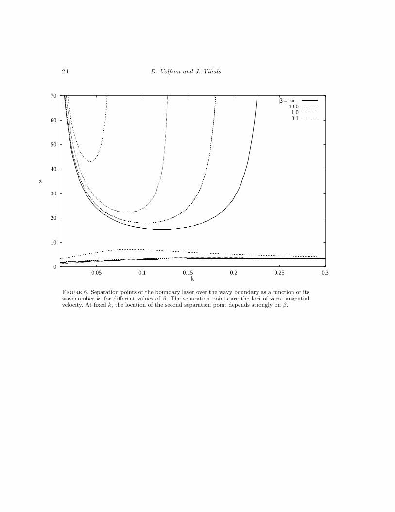
In the opposite limit of k ≪ 1 one formally recovers the Schlichting problem in thatthe characteristic longitudinal length scale is much larger than the Stokes layer thickness.There is one fundamental difference, however, which can be seen from the solution, Eq.(4.18). It has two contributions: the first one is proportional Ai, arises from the particu-lar solution,and serves to balance the non-homogeneity in Eq. (4.16). This contributiondecays within the Stokes layer. The second one is proportional to Bi, and arises from thegeneral solution of the homogeneous part of the equation. This contribution decays overthe stretched scale Z. It turns out that this second contribution introduces an additionalseparation of the composite boundary layer when 0 < k 6 0.23. The lines of zero value ofthe longitudinal component of the steady velocity profile are shown Fig. 6. The locationof the second separation point is entirely determined by that part of the solution that isproportional to Bi, and occurs at z ∼ O(1/k) ≫ 1.

The steady velocity may be obtained by expanding the exact solution (Eq. (4.18)) in

power series of k, first keeping z fixed (inner solution, u(s)1i ), and second keeping Z fixed

(outer solution u(s)1o ). To leading order, we find,

u(s)1i (z

′) ∼ −Rek2sin(kx)

[z′

2(sin(z′)− cos(z′)) + 2sin(z′) +

1

2cos(z′)

]

e−z′

+e−2z′

4−

3

4

, z′ = z/21/2 ∼ O(1), (4.22)

u(s)1o (Z) ∼ −Rek2sin(kx)

[3

4(Z − 1)e−Z

]

, Z ∼ O(1). (4.23)

The solution for the inner and outer steady velocities was already obtained by Lyne(1971) by a conformal transformation technique. We further note that the inner and outer

solutions can now be matched by requiring that u(s)1i (∞) = u

(s)1o (0) = 3/4Rek2sin(kx).

Hence it is possible to construct a uniformly valid solution by adding the inner and outersolutions, and subtracting the first term of the inner expansion of the outer solution. We


find,

u(s)1c (z

′) ∼ −Rek2sin(kx)

[z′

2(sin(z′)− cos(z′)) + 2sin(z′) +

1

2cos(z′)

]

e−z′

+e−2z′

4+

3

4(21/2kz′ − 1)e−21/2kz′

(4.24)

We now turn to a numerical study of the case of finite β. The boundary value problem(4.16) has been solved numerically by using a multiple shooting method for non stiffand linear boundary value problems (Mattheij & Staarink (1984)). The method has theadvantage that the necessary intermediate shooting points are determined by the methoditself, and that it can give the solution on a preset and nonuniform grid of points. Thecode was tested on the analytically known solution of the deterministic limit, Eqs. (4.18)and (4.19). Our results are summarized in Figs. 6, 7 and 8.Figure 6 shows the separation points of the stationary velocity as a function of the

boundary wavenumber k for a range of values of β, including for reference the deter-ministic limit of β = ∞ (separation points are defined to be the zeros of the stationarytangential velocity). This figure shows that for fixed k, the mean stationary velocity fieldmay be comprised of two or four recirculating cells per wall period depending on β. Thefirst separation point is largely independent of β, whereas the deviation of the secondrelative to its value in the monochromatic limit is proportional to β/π(1+β2), the valueof P (0, β).Our results in the limit k ≪ 1 are presented in Fig. 7, where profiles of tangential

component of the mean stationary velocity are plotted for k = 0.1 and different values ofβ. At large β (close to the monochromatic limit) the flow is comprised of four recirculatingcells per boundary period. Upon decresing β, the second separation point moves to infinity(see also Fig. 6), so that beyond some critical value of β, only two recirculating cellsremain. Further decrease in β results in the reappearance of the second separation pointat infinity, which then continues to move towards decreasing z. The intensity of therecirculating modes does not change monotonically with β as we further discuss below.

In the opposite limit of k ≫ 1 (Fig. 8 shows the case k = 10.0; note that u(s)1 is now

normalized by Re/k2), the qualitative structure of the flow is largely independent of β.The streaming flow has two recirculating cells per wall wavelength, and their intensityincreases monotonically with decreasing β.The complex dependence of the flow on β and k can be qualitatively understood

from the interplay between the width of the power spectrum (given by 1/β), the viscousdamping of each elementary excitation that depends on its frequency, and the penetra-tion depth of the flow field which is primarily dictated by the boundary wavelength. Forsmall k, large frequency modes are damped close to the boundary and do not penetratemuch into the recirculating layers. Reducing β introduces high frequency componentsinto the driving terms at first order, but they are dynamically damped. At the sametime, the power in the dominant frequency components (around Ω) decreases. Overall, adecrease in β then leads to a decrease in recirculation strength. As k increases, larger fre-quencies contribute to the flow over the entire range of the recirculating cells. Decreasingβ decreases the strength of the dominant components, but increases the range of highfrequencies that can contribute to the flow. From Eq. (4.16) one can show that the driv-ing contribution from higher frequencies which is contained in Q increases faster withfrequency than the decreasing weight given to them by the power spectrum P (ω, β).Consequently, decreasing β (which amounts to moving towards the white noise limit)leads to increasing amplitude of the recirculation.


In summary, for any value of β, finite or infinite, the vorticity produced by vibrationof the wavy boundary does not penetrate into the bulk farther than a distance of or-der of the wavelength of the boundary. However, there are qualitative differences withthe deterministic limit in the character of the flow within that layer. In particular, thestructure and the intensity of the stationary secondary flow strongly depend on β.

5. Summary

We have addressed the flow induced by a randomly vibrating solid boundary in anotherwise quiescent fluid. This analysis has been motivated by the random residual ac-celeration field in which microgravity experiments are conducted. The salient features ofthe flow are summarized below.When the solid boundary is planar, the flow field averages to zero (the average velocity

of the boundary has been taken to be zero in all cases investigated), but its variancedecays algebraically with distance away from the wall. This dependence follows from anon vanishing power spectrum of the boundary velocity at zero frequency. Introducinga low frequency cut-off in the power spectrum leads back to the classical exponentialdecay, with a rate that is determined by the cut-off frequency, Eq. (2.27). The amplitudeof the decaying variance depends explicitly on the correlation time of the boundaryvelocity, β = Ωτ , where Ω is the dominant angular frequency of the power spectrum ofthe boundary velocity, and τ is inverse spectral width (τ is the correlation time of theboundary velocity).If the solid boundary is curved, steady streaming is generated in analogy with the

classical analysis of Schlichting. The stationary part of the ensemble average of the sec-ondary velocity is nonzero, even though the boundary velocity averages to zero. In thiscase, we find that the leading contribution to the average stationary velocity divergeslogarithmically with distance away from the boundary. In analogy to the planar case,the introduction of a low frequency cut-off in the power spectrum of the boundary ve-locity changes the asymptotic behavior qualitatively. The average stationary velocityasymptotes now to a constant, given by Eq. (3.18). The asymptotic velocity explicitlydepends on β and logarithmically on the cut-off frequency. This asymptotic behavior isnot reached until a length scale of the order of the Stokes layer thickness that is basedon the cut-off frequency.We have finally analyzed the case of a periodically modulated solid boundary in the

limit in which the scale of the wall modulation is small compared to the thickness of theStokes layer, and also when the spatial amplitude of the boundary oscillation is smallcompared with the wavelength of the wall profile. Cancellation of vorticity productionover the wall boundary leads to exponential decay of the fluid velocity away from theboundary, with a decay length which is proportional to the wall wavelength, even ifthe zero frequency value of the power spectrum of the boundary velocity is nonzero. Ifthe boundary wavelength is much larger than the Stokes layer thickness, we find steadystreaming in secondary flow with two or four recirculating cells per wall period depend-ing on β. On the other hand, if the wavelength is much smaller than the Stokes layerthickness, only two recirculating cells are formed regardless of the value of β. Somewhatunexpectedly, the intensity of the recirculation can both increase or decrease with β.

This research has been supported by the Microgravity Science and Applications Divi-sion of the NASA under contract No. NAG3-1885, and also in part by the SupercomputerComputations Research Institute, which is partially funded by the U.S. Department ofEnergy, contract No. DE-FC05-85ER25000.


REFERENCES

Alexander, J.I.D. 1990 Low-gravity experiment sensitivity to residual acceleration: a review.Microgravity sci. technol. 3, 52.

Alexander, J.I.D., Garandet, J.P., Favier, J.J. & Lizee, A. 1997 g-jitter effects on seg-regation during directional solidification of tin-bismuth in the mephisto furnace facility. J.Crystal Growth 178, 657.

Alexander, J.I.D., Ouazzani, J. & Rosenberger, F. 1991 Analysis of the low gravity tol-erance of Bridgman-Stockbarger crystal growth. J. Crystal Growth 113, 21.

Batchelor, G.K. 1967 An Introduction to Fluid Dynamics. Cambridge: Cambridge UniversityPress.

Blondeaux, P. & Vittori, G. 1994 Wall imperfections as a triggering mechanism for Stokeslayer transition. J. Fluid Mech. 264, 107.

Carslaw, H.S. & Jaeger, J.C. 1959 Conduction of heat in solids. Oxford: Clarendon Press.DeLombard, R., McPherson, K., Moskowitz, M. & Hrovat, K. 1997 Comparison tools

for assessing the microgravity environment of missions, carriers and conditions. Tech. Rep.TM 107446. NASA.

Farooq, A. & Homsy, G.M. 1994 Streaming flows due to g-jitter-induced natural convection.J. Fluid Mech. 271, 351.

Gershuni, G.Z. & Lyubimov, D.V. 1998 Thermal Vibrational Convection. New York: JohnWiley & Sons.

Gershuni, G.Z. & Zhukhovitskii, E.M. 1976 Convective Stability of Incompressible Fluids.Jerusalem: Keter.

Gradshteyn, I.S. & Ryzhik, I.M. 1980 Tables of integrals, series and products. New York:Academic Press.

Grassia, P. & Homsy, G.M. 1998a Thermocapillary and buoyant flows with low frequencyjitter. I. jitter confined to the plane. Phys. Fluids 10, 1273.

Grassia, P. & Homsy, G.M. 1998b Thermocapillary and buoyant flows with low frequencyjitter. II. spanwise jitter. Phys. Fluids 10, 1291.

Kamotani, Y., Prasad, A. & Ostrach, S. 1981 Thermal convection in an enclosure due tovibrations aboard a spacecraft. AIAA J. 19, 511.

Kaneko, A. & Honjii, H. 1979 Double structures of steady streaming in the oscillatory viscousflow over a wavy wall. J. Fluid Mech. 93, 727.

Lyne, W.H. 1971 Unsteady viscous flow over a wavy wall. J. Fluid Mech. 50, 33.Mattheij, R.M.M. & Staarink, G.W.M. 1984 An efficient algorithm for solving general linear

two-point bvp. SIAM J. Sci. Stat. Comp. 5, 745.Nayfeh, A.H. 1981 Introduction to Perturbation techniques. New York: John Wiley & Sons.Nelson, E.S. 1991 An examination of anticipated g-jitter on space station and its effects on

materials processes. Tech. Rep. TM 103775. NASA.Schlichting, H. 1979 Boundary layer theory , 7th edn. New York: McGraw-Hill.Stokes, G.G. 1851 Trans. Camb. Phil. Soc. 9, 8, Mathematical and Physical Papers 3,1.Stratonovich, R.L. 1967 Topics in the Theory of Random Noise, vol. II. New York: Gordon

and Breach.Thomson, J.R., Casademunt, J., Drolet, F. & Vinals, J. 1997 Coarsening of solid-liquid

mixtures in a random acceleration field. Phys. Fluids 9, 1336.Van Dyke, M. 1964 Perturbation Methods in Fluid Mechanics. New York: Academic Press.Vittori, G. 1989 Non-linear viscous oscillatory flow over a small amplitude wavy wall J. Hydr.

Res. 27, 267.Walter, H.U., ed. 1987 Fluid Sciences and Materials Sciences in Space. New York: Springer

Verlag.Zhang, W., Casademunt, J. & Vinals, J. 1993 Study of the parametric oscillator driven by

narrow band noise to model the response of a fluid surface to time-dependent accelerations.Phys. Fluids A 5, 3147.


0

0.05

0.1

0.15

0.2

0.25

0.3

0.35

0 2 4 6 8 10 12 14 16 18 20z

I(z,β) z2 β=5

β=10

β=100

Figure 1. Normalized variance of the tangential velocity for the case of a planar boundary com-puted by numerical integration of Eq. (2.21) (symbols), and its uniform asymptotic expansion,Eq. (2.23), (solid lines). The function I(z, β) z2 asymptotes to a constant value outside of theclassical Sokes layer based on Ω. The uniform expansion remains a good approximation even formoderate β.


-1.4

-1.2

-1

-0.8

-0.6

-0.4

-0.2

0

0.2

0 5 10 15 20 25 30 35 40z

∂zψ1(s)( z )

β = ∞ 100.0 10.0 1.0

Figure 2. Stationary first order velocity as a function of distance for a range of values of β. Allcurves diverge logarithmically at large z, except for β = ∞ (monochromatic limit), in which thevelocity asymptotes to a constant within the Stokes layer. This latter behavior reproduces theclassical result of Schlichting.


-1

-0.8

-0.6

-0.4

-0.2

0

0.2

0 5 10 15 20 25 30 35 40z

∂zψ1(s)( z )

β = ∞10.0 1.0 0.1

Figure 3. Stationary first order velocity as a function of distance for a range of values of β. Thepower spectrum of the boundary velocity has a low frequency cut-off at ωc = 0.05. The velocityasymptotes to a constant that depends on the value of β.


-1

-0.9

-0.8

-0.7

-0.6

0 0.1 0.2 0.3 0.4 0.5

ωc

u1(s)( z = ∞)

numericalanalical

Figure 4. Asymptotic dependence of the stationary velocity as a function of the cut-off fre-quency ωc. We show the case β = 10 given by Eq. (3.18) along with the numerically obtainedsolution.


≈

u(x, ∞, t) = (u0(t), 0)

x

z

Figure 5. Schematic view of the geometry of the wavy wall studied in Section 4.


0

10

20

30

40

50

60

70

0.05 0.1 0.15 0.2 0.25 0.3k

z

β = ∞ 10.0 1.0 0.1

Figure 6. Separation points of the boundary layer over the wavy boundary as a function of itswavenumber k, for different values of β. The separation points are the loci of zero tangentialvelocity. At fixed k, the location of the second separation point depends strongly on β.


-0.3

-0.2

-0.1

0

0.1

0.2

0.3

0 10 20 30 40 50

z

k=0.1

u1(s)(π/2k ,z)

Re k2

analytic solution, β= ∞numerical solution, β=9.1

β=2.1 β=1.1 β=0.1

Figure 7. Tangential component of the mean stationary velocity as a function of z for k = 0.1and a range of values of β. The case β = ∞ corresponds to analytic solution obtained by Lyne.The other curves are the numerical solutions of the boundary value problem defined by Eq.(4.16) and corresponding boundary conditions.


-0.3

-0.2

-0.1

0

0.1

0.2

0.3

0 0.2 0.4 0.6 0.8 1

z

u1(s)(π/2k ,z)

(Re / k2)

k=10.0

analytic solution, β= ∞numerical solution, β=5.0

β=2.5 β=1.5 β=0.5

Figure 8. Tangential component of mean stationary velocity as a function of z for k = 10 anda range of values of β. The case β = ∞ corresponds to analytic solution obtained by Lyne. Theother curves are the numerical solutions of the boundary value problem defined by Eq. (4.16)and corresponding boundary conditions.

flow induced by a randomly vibrating boundary - arxiv · flow induced by a randomly vibrating...

Documents