flow regime transition criteria for two-phase flow at...

1

Flow regime transition criteria for two-phase flow at

reduced gravity conditions

R. Situa*, T. Hibikib, R. J. Brownc, T. Hazukud and T. Takamasad

a School of Engineering and Physical Sciences, James Cook University, Townsville,

QLD 4811, Australia.

b School of Nuclear Engineering, Purdue University, 400 Central Drive, West Lafayette,

IN 47907-2017, USA.

c Faculty of Built Environment and Engineering, Queensland University of Technology, 2

George Street, Brisbane, QLD 4001, Australia.

d Graduate School of Marine Science and Technology, Tokyo University of Marine

Science and Technology, 2-1-6 Etsujima, Koto 135-8533, Tokyo, Japan.

*Corresponding author: Tel: +61-7-47814172, Fax: +61-7-47816788, Email:

[email protected]

2

Abstract

Flow regime transition criteria are of practical importance for two-phase flow analyses at

reduced gravity conditions. Here, flow regime transition criteria which take the frictional

pressure loss effect into account were studied in detail. Criteria at reduced gravity

conditions were developed by extending an existing model from normal gravity to

reduced gravity conditions. A comparison of the newly developed flow regime transition

criteria model with various experimental datasets taken at microgravity conditions

showed satisfactory agreement. Sample computations of the model were performed at

various gravity conditions, such as 0.196, 1.62, 3.71 and 9.81 m/s2 corresponding to

micro-gravity and lunar, Martian and Earth surface gravity, respectively. It was found

that the effect of gravity on bubbly−slug and slug−annular (churn) transitions in a two-

phase flow system was more pronounced at low liquid flow conditions, whereas the

gravity effect could be ignored at high mixture volumetric flux conditions. While for the

annular flow transitions due to flow reversal and onset of droplet entrainment, higher

superficial gas velocity was obtained at higher gravity level.

Keywords: Flow regime; Transition; Reduced gravity; Microgravity; Multiphase flow;

Two-phase flow.

3

1. Introduction

With the advent of modern cooling systems, the increasing demand to meet stringent

weight- and space-saving design parameters for large spacecraft such as the International

Space Station requires extensive heat removal to ensure acceptable internal

environmental conditions. This cannot be accomplished by conventional single-phase

forced or natural convection flows. Hence two-phase thermal systems have been

developed with forced convective boiling flows which have a controllable heated surface

temperature to yield a relatively high heat transfer coefficient and the possibility of

meeting compact space requirements (Grigoriev et al., 1996). In view of the great

importance of this to the thermal−hydraulic design of thermal-control systems at reduced

gravity conditions, a number of experiments have been performed for two-phase flow at

reduced gravity conditions by means of a drop tower or an aircraft (Heppner et al., 1975;

Dukler et al., 1988; Colin et al., 1991; Zhao and Rezkallah, 1993; Bousman et al., 1996;

Choi et al., 2003; Takamasa et al., 2003, 2004). In these experiments, the measured

essential two-phase flow characteristics included flow regime, void fraction, and

interfacial area concentration.

The internal structures of the two-phase flow are classified by the flow regimes or

flow patterns. Transfer mechanisms between the two-phase mixture and the wall, as well

as between the phases, depend on the flow regimes. This leads to the use of regime−

dependent correlations together with two-phase flow regime criteria. The basic structure

of the two-phase flow can also be characterized by two fundamental geometrical

parameters: void fraction and interfacial area concentration. The former expresses the

phase distribution and is a required parameter for both the drift-flux model, one of the

most practical and accurate models for hydrodynamic and thermal design in various

industrial processes, and the two-fluid model, which describes in detail the

thermal−hydraulic transients and phase interactions. In the two-fluid model, the main

difficulties arise from the existence of interfaces between the phases and the associated

discontinuities. Hence interfacial area was introduced to describe the available area for

the interfacial transfer of mass, momentum and energy, which is modeled in the

interfacial area transport model, a crucial complement of the two-fluid model.

4

The application of the drift-flux and two-fluid models as well as of the interfacial

area transport equation in reduced gravity conditions has enjoyed great success recently.

In the drift-flux model, the constitutive equations of the distribution parameter for bubbly

flow, which takes the gravity effect into account, have been proposed. The constitutive

equations for slug, churn and annular flows, which can be applicable to reduced gravity

conditions, have also been recommended based on existing experimental and analytical

studies. The second essential parameter, drift velocity, was modeled by taking frictional

pressure loss into account in various flow regimes (Hibiki et al., 2006). On the other hand,

the interfacial area transport equation was also extended to reduced gravity conditions.

The constitutive equation for the sink term due to wake entrainment was formulated by

considering body acceleration due to frictional pressure loss. The newly-developed

interfacial area transport equation agreed satisfactorily with experimental data taken at

normal and reduced gravity conditions (Hibiki et al., 2009).

In the thermal−hydraulic system analysis codes developed in a normal gravity

environment, the effects of interfacial structure were analyzed by using models of flow

regime transition criteria. Some of these models were extended to microgravity

conditions with some success. For example, the model by Dukler et al. (1988), based on

the critical void fraction at both bubbly−slug and slug−annular transitions, appeared to

agree well with the experimental data. Lee et al. (1987) suggested that the bubbly−slug

transition happens when the force of eddy turbulent fluctuation is greater than the surface

tension force, and slug−annular transition occurs when the inertial force is greater than

the surface tension force. The latter criterion led to the Weber number based model

proposed by Rezkallah and his colleagues (Zhao and Rezkallah, 1993; Rezkallah and

Zhao, 1995; Rezkallah, 1996; Lowe and Rezkallah, 1999). However, the Dukler et al.

model depends on the estimation of the area-averaged void fraction, α, which has to be

adjusted to fit for different fluids and pipe sizes (Bousman et al., 1996; Zhao and

Rezkallah, 1993). Moreover, few churn flow in microgravity conditions has been

reported. Instead, models of slug−annular transition have been proposed to cover this

broad range. Most importantly, no general models on various gravity levels, such as the

lunar and Martian levels, exist.

5

Acknowledging the importance of the flow regime transition criteria models

under reduced gravity conditions, this study presents an extensive survey of existing

models and data at reduced gravity conditions, and extends the well-established Mishima

and Ishii (M−I) model at normal gravity conditions (Mishima and Ishii, 1984) to reduced

gravity conditions. The proposed model with its large datasets of different fluid property

and pipe sizes is also evaluated. Furthermore, a feasibility study is performed to apply the

new model to other gravity conditions such as the lunar and Martian gravity levels.

2. Literature survey

2.1 Existing data of the flow regime transition boundary in two-phase flow at reduced

gravity conditions

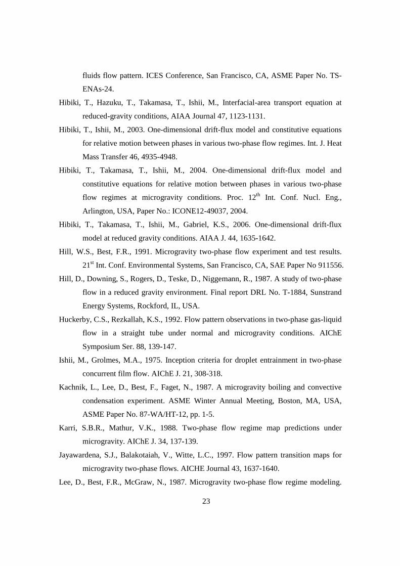
Table 1 summarizes the experimental investigations of the two-phase flow regime under

microgravity conditions that have been performed since the 1970s (Heppner et al., 1975).

Most of the experiments were conducted on parabolic flights such as in KC-135, MU-300,

Learjet and IL-76, since they could provide about 20 s of microgravity conditions. Dukler

et al. (1988) performed the tests in a 30-m drop tower, with only 2.2 s of reduced gravity.

The best environment is space and an experiment was performed by Zhao et al. (2001a)

on board the Russian space station MIR. In addition, a few tests attempted to use two

immiscible liquids with near equal densities (Karri and Mathur, 1988; Vasavada et al.,

2007) or capillary tubes (Galbiati and Andreini, 1994) under normal gravity to simulate

microgravity conditions. According to Brauner (1990), the criterion for a capillary tube

system to be an equivalent microgravity system is Bond number 62

G <∆

≡σ

ρ DgBo ,

where ∆ρ is the density difference between phases, gG is the gravitational body

acceleration (=9.81 m/s2 on the Earth’s surface, and 0 m/s2 at zero gravity), D is the pipe

diameter, and σ is the surface tension. The Bond number in Galbiati and Andreini’s

capillary tube experiment is around 0.13, which is in the microgravity range.

Both adiabatic (non-boiling) and diabatic (boiling) datasets are available in the

literature. For adiabatic flow, the majority of the research has used air−water systems,

including round tube (Colin and Fabre, 1995; Huckerby and Rezkallah, 1992) and square

channel (Zhao et al., 2001b). Other investigators used water/glycerin to study the effect

6

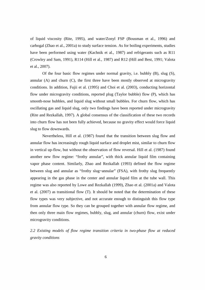
of liquid viscosity (Rite, 1995), and water/Zonyl FSP (Bousman et al., 1996) and

carbogal (Zhao et al., 2001a) to study surface tension. As for boiling experiments, studies

have been performed using water (Kachnik et al., 1987) and refrigerants such as R11

(Crowley and Sam, 1991), R114 (Hill et al., 1987) and R12 (Hill and Best, 1991; Valota

et al., 2007).

Of the four basic flow regimes under normal gravity, i.e. bubbly (B), slug (S),

annular (A) and churn (C), the first three have been mostly observed at microgravity

conditions. In addition, Fujii et al. (1995) and Choi et al. (2003), conducting horizontal

flow under microgravity conditions, reported plug (Taylor bubble) flow (P), which has

smooth-nose bubbles, and liquid slug without small bubbles. For churn flow, which has

oscillating gas and liquid slug, only two findings have been reported under microgravity

(Rite and Rezkallah, 1997). A global consensus of the classification of these two records

into churn flow has not been fully achieved, because no gravity effect would force liquid

slug to flow downwards.

Nevertheless, Hill et al. (1987) found that the transition between slug flow and

annular flow has increasingly rough liquid surface and droplet mist, similar to churn flow

in vertical up-flow, but without the observation of flow reversal. Hill et al. (1987) found

another new flow regime: “frothy annular”, with thick annular liquid film containing

vapor phase content. Similarly, Zhao and Rezkallah (1993) defined the flow regime

between slug and annular as “frothy slug−annular” (FSA), with frothy slug frequently

appearing in the gas phase in the center and annular liquid film at the tube wall. This

regime was also reported by Lowe and Rezkallah (1999), Zhao et al. (2001a) and Valota

et al. (2007) as transitional flow (T). It should be noted that the determination of these

flow types was very subjective, and not accurate enough to distinguish this flow type

from annular flow type. So they can be grouped together with annular flow regime, and

then only three main flow regimes, bubbly, slug, and annular (churn) flow, exist under

microgravity conditions.

2.2 Existing models of flow regime transition criteria in two-phase flow at reduced

gravity conditions

7

Modeling of two-phase flow regime transition at reduced gravity has been developed

along with the construction of microgravity databases (Zhao and Hu, 2000). Proposed

models in the literature include a void fraction based model (Dukler et al., 1988), a force

balance based model (Lee et al., 1987), a Weber number based model (Zhao and

Rezkallah, 1993), and a dimensionless number model (Jayawardena et al., 1997).

Dukler et al. (1988) assumed that at bubbly−slug transition, liquid velocity equals

gas velocity, and adjacent bubbles contact each other, which gives a void fraction of 0.45,

and

gf 22.1 jj = , (1)

where jf and jg are superficial liquid velocity and superficial gas velocity respectively.

Similarly, Colin et al. (1991) and Zhao and Rezkallah (1993) empirically determined the

critical void fraction to be 0.20 and 0.18, respectively, with the assumption of zero drift

velocity giving

gf 2.3 jj = , (2)

and

gf 56.4 jj = . (3)

For the slug−annular transition criteria, Dukler et al. (1988) equated the area-

averaged void fraction in slug flow (estimated from the distribution parameter C0 in the

drift-flux model) with that in annular flow (estimated based on force balance on the liquid

film). Similarly, Lee et al. (1987) conducted theoretical force balance analysis on four

basic horizontal flow patterns: dispersed, slug, stratified and annular. They claimed that

transition from other flow to stratified flow occurs when body force overcomes surface

tension (superficial liquid velocity less than 0.01 m/s), transition from slug to dispersed

flow occurs when eddy turbulent fluctuation is higher than surface tension, and transition

from slug to annular takes place if inertial force dominates surface tension. The last

criterion was also deduced for the Weber number model (Zhao and Rezkallah, 1993),

since the Weber number is the ratio of inertial force over surface tension. According to

Zhao and Rezkallah (1993), the transition from slug to FSA occurs at

12gg

sg =≡σ

ρ DjWe , (4)

8

where ρg is the gas density. The transition from FSA to annular happens at

20sg =We , (5)

Similarly, other investigators (Jayawardena et al., 1997) attempted to find

transition lines on a flow pattern map using a dimensionless number such as a Suratman

number (Su ≡ Resf2/Wesf) as well as gas and liquid Reynolds numbers:

Bubbly−slug transition: 32

sf

sg 16464 /Su.Re

Re −= , when 104 < Su < 107 (6)

Slug−annular transition: 32

sf

sg 64641 /Su.Re

Re −= , for Su < 106

29sg 102 SuRe −×= , for Su > 106

(7)

where gas and liquid Reynolds numbers are defined as Resf ≡ ρfjf D/µf and Resg ≡ ρgjg D/jg,

respectively.

3. Modeling of flow regime transition criteria in two-phase flow at reduced gravity

conditions

3.1 Body acceleration due to the frictional pressure drop

Under microgravity conditions, the gravity force which pushes a gas phase faster than a

liquid phase becomes negligible. This major difference between microgravity and normal

gravity led to the assumption adopted by some researchers that there was no local slip

between bubble and liquid. However, Tomiyama et al. (1998) found through theoretical

analysis that the relative velocity between a single bubble and liquid flow in a confined

channel exists and is driven by a frictional pressure gradient due to a liquid flow. This

was confirmed by bubbly flow experiments at low liquid Reynolds numbers (Takamasa

et al., 2004). This single particle system was extended to a multiple-particle system,

where the actual body acceleration, gB, on the gas phase consists of the body acceleration

due to the frictional pressure drop at the wall, gF (Hibiki and Ishii, 2003):

( )αρ −∆+=+=

1F

GFGB

Mgggg , (8)

where α is the area-averaged void fraction, and MF is the frictional pressure gradient in a

multi-particle system, given by

9

∞=

−≡ F2fF Φ

d

dM

z

pM , (9)

where 2fΦ is the two-phase multiplier calculated by Lockhart-Martinelli’s (1949)

correlation, and MF∞ is the frictional pressure gradient in a confined channel flow with a

single bubble, approximated by

2ffF 2

vD

fM ρ=∞ , (10)

where f is the wall friction factor.

Recently, the relative motion between gas and liquid phases has been successfully

modeled by taking into account the effect of a frictional pressure gradient caused by a

liquid flow (Hibiki et al. 2006):

Bubbly flow

( ) ( ) ( )

( ) ( )

2 G F1 4

G FG F3 72

f 6 7 G F

G F

118 67 1

21

1 17 67 1

.

.

gj

g M

g Mg MV

g M

g M

∆ρ αα

∆ρ∆ρ σρ ∆ρ α

α∆ρ

∞∞

∞

− + − ++ = ×

− + + − +

, (11)

Slug flow

( )[ ]( )

21

f

FGgj 1

135.0

−+−∆

=αρ

αρ DMgV , (12)

Churn flow

( )[ ] 41

2f

FGgj

12

+−∆

=ρ

σαρ MgV , (13)

Annular flow

0gj ≈V . (14)

where Vgj is the void-fraction weighted area-average drift velocity.

3.2 Body acceleration considering frictional pressure loss in forced convective flow

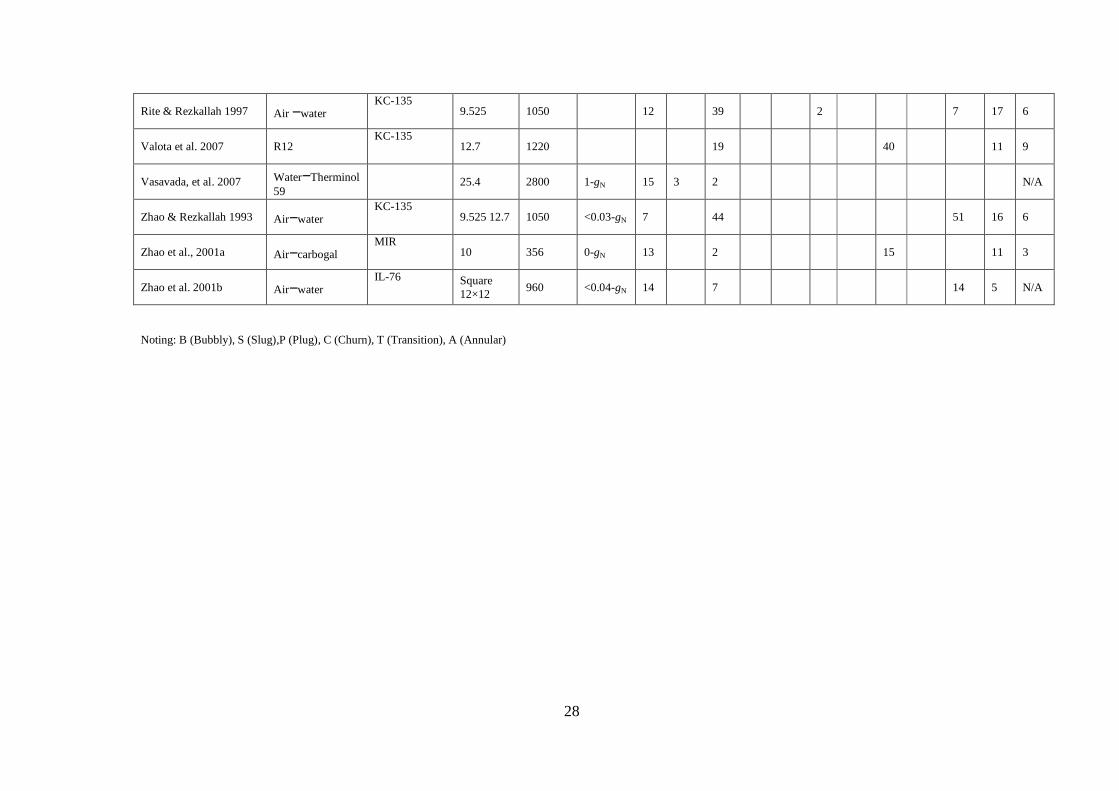
For a relatively high mixture-volumetric-flux condition, the actual body acceleration is

much higher than the normal gravity acceleration. Figure 1 presents the ratio of actual

body acceleration over gravitational body acceleration, gB/gG, versus the superficial gas

10

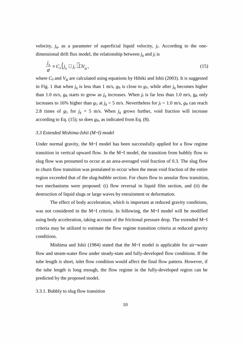
velocity, jg, as a parameter of superficial liquid velocity, jf. According to the one-

dimensional drift flux model, the relationship between jg and jf is

( ) gjfg0g VjjC

j++=

α, (15)

where C0 and Vgj are calculated using equations by Hibiki and Ishii (2003). It is suggested

in Fig. 1 that when jg is less than 1 m/s, gB is close to gF, while after jg becomes higher

than 1.0 m/s, gB starts to grow as jg increases. When jf is far less than 1.0 m/s, gB only

increases to 16% higher than gG at jg = 5 m/s. Nevertheless for jf = 1.0 m/s, gB can reach

2.8 times of gG for jg = 5 m/s. When jg grows further, void fraction will increase

according to Eq. (15); so does gB, as indicated from Eq. (8).

3.3 Extended Mishima-Ishii (M−I) model

Under normal gravity, the M−I model has been successfully applied for a flow regime

transition in vertical upward flow. In the M−I model, the transition from bubbly flow to

slug flow was presumed to occur at an area-averaged void fraction of 0.3. The slug flow

to churn flow transition was postulated to occur when the mean void fraction of the entire

region exceeded that of the slug-bubble section. For churn flow to annular flow transition,

two mechanisms were proposed: (i) flow reversal in liquid film section, and (ii) the

destruction of liquid slugs or large waves by entrainment or deformation.

The effect of body acceleration, which is important at reduced gravity conditions,

was not considered in the M−I criteria. In following, the M−I model will be modified

using body acceleration, taking account of the frictional pressure drop. The extended M−I

criteria may be utilized to estimate the flow regime transition criteria at reduced gravity

conditions.

Mishima and Ishii (1984) stated that the M−I model is applicable for air−water

flow and steam-water flow under steady-state and fully-developed flow conditions. If the

tube length is short, inlet flow condition would affect the final flow pattern. However, if

the tube length is long enough, the flow regime in the fully-developed region can be

predicted by the proposed model.

3.3.1. Bubbly to slug flow transition

11

Figure 2(a) shows a schematic diagram of bubbly−slug transition models under reduced

gravity conditions. Mishima and Ishii (1984) adopted the assumption that coalescence

occurs when the gap between two bubbles is less than a bubble diameter Db, which leads

to the sphere of influence being 1.5 Db. Hence the critical void fraction at the transition is

given by

( )3.0296.0

5.1 3b

3b ≈==

D

Dα . (16)

This assumption still holds under reduced gravity conditions. In addition, by taking

account of the frictional pressure drop, the void-fraction-weighted drift velocity is

modified as (Hibiki et al. 2006)

( )( ) ( )

( ) ( ) 7/3

F

F7/6

F

F24/1

2f

Fgj

1167.171

1167.18

2

+∆+−∆

−+

+∆+−∆

−

+∆=

∞

∞∞

Mg

Mg

Mg

Mg

MgV

ραρα

ραρα

ρσρ

. (17)

Note that this criterion is not applicable in some situations where bubbles cannot freely

pack with each other, such as flows in extremely small diameter pipe.

3.3.2. Slug to annular (churn) flow transition

Mishima and Ishii (1984) attempted to find the mean void fraction in the slug bubble

section and equate it to the mean void fraction over the entire region. At first, potential

flow analysis was adopted to estimate the mean void fraction of the slug bubble section.

However, the wall friction effect on the liquid flow was not considered. By considering

body acceleration due to friction pressure drop, the Bernoulli equation of the flow field

around the slug bubble in Fig. 2b becomes

( )[ ] hgvfB

22r 0

2ρα

ρ∆=− , (18)

where vr is bubble relative velocity, and h is distance from the nose of a slug bubble. The

resultant local void fraction at a distance from the nose becomes

( )( ) fB0fB

fB

35.012

2

ρρρρρρ

αDgjChg

hgh

∆+−+∆∆

= , (19)

12

where D is the hydraulic diameter of a pipe.

Secondly, to find the length of a slug bubble, Mishima and Ishii applied force

balance to the liquid film around the slug bubble. The force consisted of gravity force and

wall friction:

( )sbG2fsbf 1

3

2

2αρπρ −∆= AgDv

f, (20)

where vfsb is the terminal film velocity in the slug bubble section, and αsb is the void

fraction corresponding to the terminal film velocity. This equation is not modified here

because it already took account of the effect of gravity on the wall shear. Furthermore, Eq.

(20) also suggests that the terminal film velocity becomes zero under zero gravity

condition. This assumption is reasonable, because there is actually no force pushing the

liquid film flow downwards.

The final transition criterion is modified as

( )

75.0

18/1

2ff

3G

2/1

f

G

fB0m

75.0

35.01813.01

∆

∆+

∆+−−≥

νρρ

ρρ

ρραDgDg

j

DgjC. (21)

Under normal or reduced gravity conditions, where churn flow occurs, Eq. (21) can be

used to predict the transition between slug and churn flow. Nonetheless under

microgravity, as explained earlier, churn flow regime is replaced by other regimes such

as frothy slug−annular (Zhao and Rezkallah, 1993) or transitional flow (Zhao et al.,

2001a; Valota et al., 2007), and hence can be grouped with annular flow. So the transition

criterion in Eq. (21) can be deemed as the transition between slug and annular (churn)

flow.

3.3.3. Annular flow transition due to flow reversal

Although down-flow of liquid film along large bubbles would not happen at zero-gravity

conditions, it can still occur under reduced-gravity situations. At these environments, i.e.,

Moon or Mars, churn flow regime could exist, and the transition between churn and

13

annular due to flow reversal in the liquid film could happen. Mishima and Ishii (1984)

gave the criterion as

( )11.0g

Gg −

∆= α

ρρ Dg

j . (22)

In extending this transition to reduced gravity conditions, the gravity term, gG, in Eq. (22)

is not replaced by gB because the body acceleration due to the frictional pressure drop

becomes zero at flow reversal conditions (jf = 0).

Combining Eq. (22) with drift flux model, the final transition curve can be

obtained in the final form

∆−

+=

DgVjCj

G

g

gj0g

111.0

ρρ

, (23)

where the void-fraction weighted area-average drift velocity is calculated with Eq. (12),

which will be different from the original M−I model.

3.3.4. Annular-mist flow transition due to onset of droplet entrainment

As explained earlier, no flow reversal happens under zero- or micro-gravity conditions.

Thus, the criterion for the churn to annular transition discussed in Section 3.3.3 would not

hold. On the other hand, another criterion due to the destruction of liquid slugs or large

waves by entrainment or deformation proposed by Mishima and Ishii (1984) remains

sound. As is shown in Fig. 2c, entrainment happens when the drag force on the liquid

wave crest from the gas-shearing flow exceeds the surface tension force

σd FF ≥ . (24)

After introducing non-dimensional parameters, Ishii and Grolmes (1975) obtained the

transition criterion as

0.2µf

41

2g

Gg

−

∆≥ Ng

jρ

ρσ, (25)

where

14

2/1

Gffµf

∆≡

ρσσρµ

gN (26)

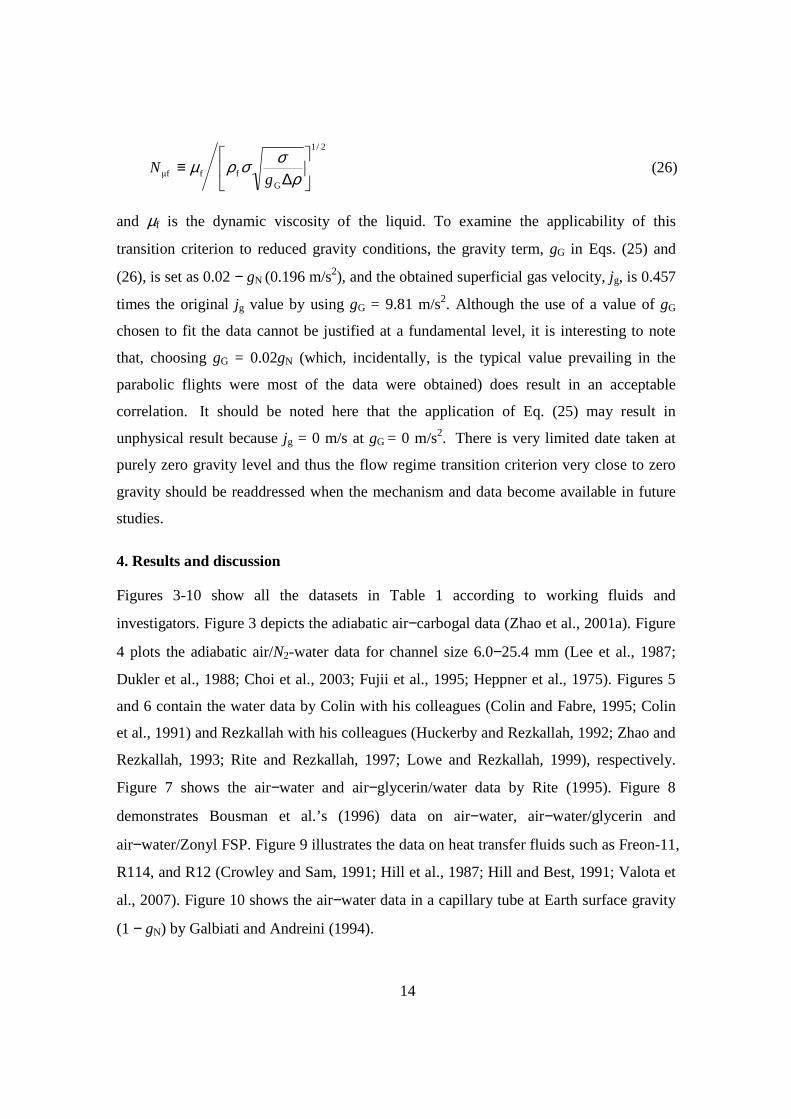
and µf is the dynamic viscosity of the liquid. To examine the applicability of this

transition criterion to reduced gravity conditions, the gravity term, gG in Eqs. (25) and

(26), is set as 0.02 − gN (0.196 m/s2), and the obtained superficial gas velocity, jg, is 0.457

times the original jg value by using gG = 9.81 m/s2. Although the use of a value of gG

chosen to fit the data cannot be justified at a fundamental level, it is interesting to note

that, choosing gG = 0.02gN (which, incidentally, is the typical value prevailing in the

parabolic flights were most of the data were obtained) does result in an acceptable

correlation. It should be noted here that the application of Eq. (25) may result in

unphysical result because jg = 0 m/s at gG = 0 m/s2. There is very limited date taken at

purely zero gravity level and thus the flow regime transition criterion very close to zero

gravity should be readdressed when the mechanism and data become available in future

studies.

4. Results and discussion

Figures 3-10 show all the datasets in Table 1 according to working fluids and

investigators. Figure 3 depicts the adiabatic air−carbogal data (Zhao et al., 2001a). Figure

4 plots the adiabatic air/N2-water data for channel size 6.0−25.4 mm (Lee et al., 1987;

Dukler et al., 1988; Choi et al., 2003; Fujii et al., 1995; Heppner et al., 1975). Figures 5

and 6 contain the water data by Colin with his colleagues (Colin and Fabre, 1995; Colin

et al., 1991) and Rezkallah with his colleagues (Huckerby and Rezkallah, 1992; Zhao and

Rezkallah, 1993; Rite and Rezkallah, 1997; Lowe and Rezkallah, 1999), respectively.

Figure 7 shows the air−water and air−glycerin/water data by Rite (1995). Figure 8

demonstrates Bousman et al.’s (1996) data on air−water, air−water/glycerin and

air−water/Zonyl FSP. Figure 9 illustrates the data on heat transfer fluids such as Freon-11,

R114, and R12 (Crowley and Sam, 1991; Hill et al., 1987; Hill and Best, 1991; Valota et

al., 2007). Figure 10 shows the air−water data in a capillary tube at Earth surface gravity

(1 − gN) by Galbiati and Andreini (1994).

15

Figures 3-10 also compare the microgravity data with the predictions by the

present model (red thick curves) and other existing models at microgravity (~0 − gN)

conditions on the jg−jf plane. As is shown by arrows in Fig. 3, the bubbly to slug

transition “B−S” is shown in red thick solid curve, the slug to annular (churn) “S−A(C)”

transition is drawn as red thick dash curves, and both have a slope close to 45°. The

annular-mist flow transition (due to droplet entrainment) calculated with Eq. (25) is

plotted with red thick dash-dot line located at the top right on the flow regime map.

According to Mishima and Ishii (1984), this transition is actually between slug and

annular (mist) flows, “S−A(M)”, rather than between churn and annular flow. In

summary, these three curves can predict the transitions between bubbly, slug, and annular

flows.

The other existing models are also shown in the figures. Eqs. (1)–(3) are located

with thin purple short-dash, magenta dot, and cyan short-dash-dot lines, respectively,

with a 45° inclination. The predictions by Eqs. (4) and (5) are shown by two vertical lines

(grey solid line: S-FSA transition, black dash line: FSA−A transition). In addition, the

B−S transition prediction by Eq. (6) is a blue dash-dot line parallel to Eqs. (1)–(3).

Finally, the S−A transition (green dash-dot-dot line) predicted by Eq. (7), depending on

the value of Su, is either an inclined line in Fig. 3a–d or a vertical line in Fig. 3e–f. The

legends of the transition curves in Figs. 4–10 are the same as those in Fig. 3. Note that the

B−S transition curves predicted by the present model and Eqs. (1), (2) (3) and (6) are not

shown in Figure 10 because they are not suitable for capillary tubes due to the reason

explained in Section 3.3.1, and only data of slug and annular regimes are plotted.

4.1 Comparison of the present model with existing models and datasets

4.1.1. Bubbly to slug flow transition

A total of six models of the bubbly−slug transition are plotted on jf vs. jg map. Eqs. (1)–

(3) do not depend on any other parameters and are 45°-angle lines, with Eq. (3) on the

left, Eq. (2) in the middle, and Eq. (1) on the right. In addition, the B−S transition curve

predicted by Eq. (6) is also parallel to these three equations, since it can be rewritten as

16

g32

g

ff 16464

1jSu

.j /

=

νν

, (27)

which is also subject to fluid properties and pipe diameter. Similarly, the predicted curve

of the present model at 0 − gN is almost parallel to them, but it deviates from 45° to the

right when superficial gas velocity decreases. From the drift flux model, the superficial

liquid velocity can be found as

gjg0

f 11

VjC

j −

−=

α. (28)

If the first term on the right hand side of Eq. (28) is dominant, jf will be proportional to jg,

and the curve on the jg–jf plane will have a slope of 45°. However, because of the

existence of the frictional pressure gradient, the drift velocity would not be equal to zero

at 0 − gN conditions. Thus the predicted curve of the present model on the jg–jf plane will

deviate to the right when superficial gas velocity decreases.

Figures 3-9 show that the present model agrees generally well with the

experimental data at the B−S transition. Nevertheless, among other existing models, the

line of Eq. (1) is closest to the present model and fits the data rather better than other

models. The line of Eq. (6) has poor agreement with the Freon data in Fig. 9.

4.1.2. Slug to annular (churn) flow transition

As is shown in Figs. 3-10, the prediction by Eq. (4) (Zhao and Rezkallah, 1993) of S-to-

FSA transition is a vertical solid line on the jg−jf plane because the transition is assumed

to depend on a Weber number, which is only subject to superficial gas velocity. The

prediction by Eq. (7) (Jayawardena et al., 1997) on a broader S−A transition is a vertical

or a 45° dash-dot-dot line depending on Su value. Similarly, the prediction of the present

model at 0 − gN for the S−C transition is approximately parallel to that for the B−S

transition, due to the same reason explained in the last section. However, the slope

difference between the present model and Eq. (7) is more significant for capillary tube

data at 1 - gN.

In Figs. 3-10, only two data points of churn flow are plotted, as in Fig. 4 (c). As

explained in Section 2.1, the slug to churn transition is actually the transition between

17

slug to annular (churn) flow. The agreement between the present model and the various

datasets is fairly good. In addition, Jayawardena et al.’s (1997) correlation was developed

using the air−water and Freon datasets, and generally agrees with the majority of the data,

except air−carbogal data and 1 − gN capillary tube data. Moreover, Zhao and Rezkallah’s

model of the S-FSA transition in Eq. (4) agrees well with their own data in Figs. 6 and 7,

but tends to underestimate compared with other datasets.

4.1.3. Slug to annular-mist flow transition

The prediction by the present model on the S−A transition at 1 - gN does not depend on jf,

as shown in Eq. (25). Rather it is represented by a vertical line. Since the contribution of

gravity to the actual body acceleration is negligible for the S−A(M) transition, the

original M−I model is not changed, and the value of 0.02 gG is chosen for gG for

microgravity conditions because majority of the experiments in literature were performed

at parabolic flight. Existing model being compared is Eq. (5) (Zhao and Rezkallah, 1993)

on the FSA−A transition at 0 − gN, which is mostly located on the right of the present

model, except for large pipe diameter (D ≥19 mm) in air−water condition and data of

R114 and R12 in Fig. 9. Nevertheless, when Su > 106, Jayawardena et al.’s (1997)

prediction on slug to annular transition also gives a vertical line, which is on the left of

the line of Eq. (5), except for Fig. 3 (d) which has a pipe size of 40 mm. For cases where

Su < 106, the 45° line predicted by Jayawardena et al. (1997) is hard to compare with the

present S−A(M) models.

Figures 3-10 show that the present model generally agrees well with the majority

of existing datasets. Annular-mist flow and roll wave in microgravity have been observed

by several researchers (Bousman, et al. 1996; Zhao and Rezkallah, 1993; Dukler et al.

1988). There is a plenty of evidence of the occurrence of entrainment in microgravity.

Zhao and Rezkallah’s model in Eq. (5) of the FSA−A transition fits well with their own

data in Figs. 4 and 5-(a), but over-predicts against other databases.

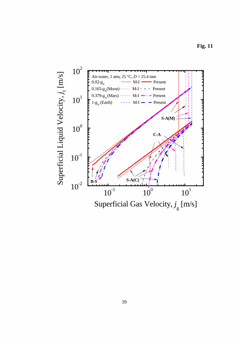
4.2 Sample computation of the present model at reduced gravity conditions

To examine the effect of gravity on two-phase flow regime transition, sample

computations of the present model (thick lines) and the original M−I model (thin lines)

18

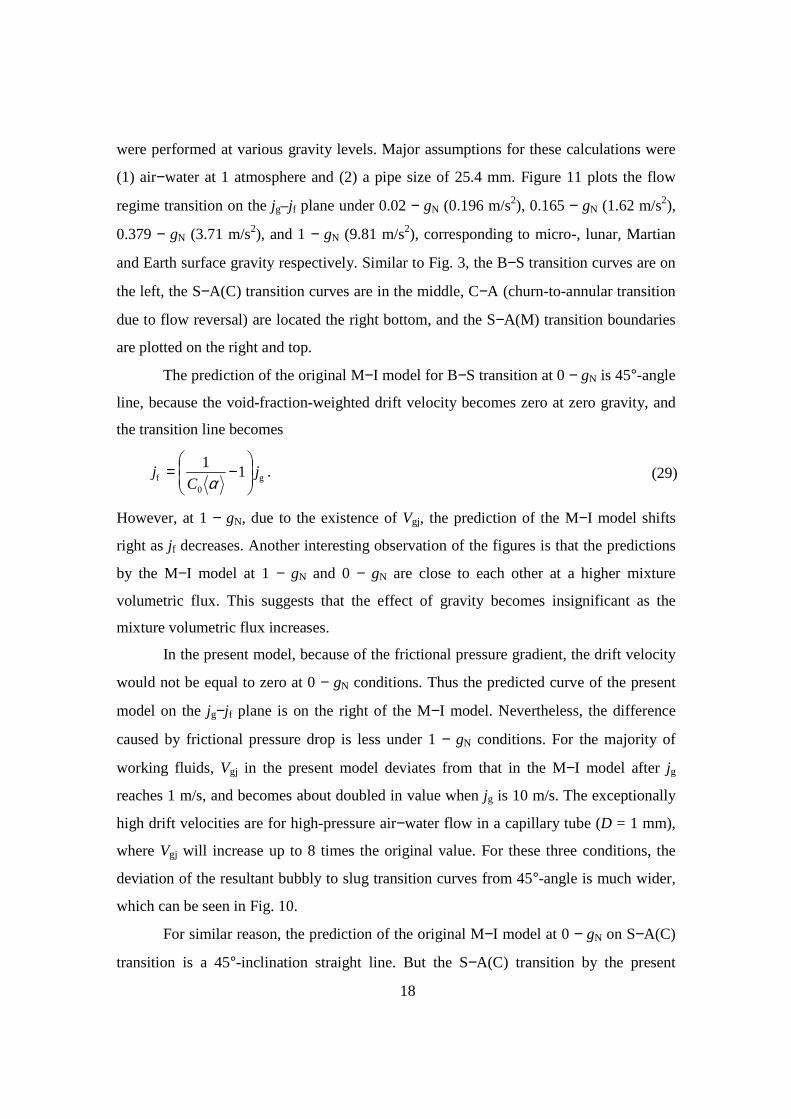
were performed at various gravity levels. Major assumptions for these calculations were

(1) air−water at 1 atmosphere and (2) a pipe size of 25.4 mm. Figure 11 plots the flow

regime transition on the jg–jf plane under 0.02 − gN (0.196 m/s2), 0.165 − gN (1.62 m/s2),

0.379 − gN (3.71 m/s2), and 1 − gN (9.81 m/s2), corresponding to micro-, lunar, Martian

and Earth surface gravity respectively. Similar to Fig. 3, the B−S transition curves are on

the left, the S−A(C) transition curves are in the middle, C−A (churn-to-annular transition

due to flow reversal) are located the right bottom, and the S−A(M) transition boundaries

are plotted on the right and top.

The prediction of the original M−I model for B−S transition at 0 − gN is 45°-angle

line, because the void-fraction-weighted drift velocity becomes zero at zero gravity, and

the transition line becomes

g0

f 11

jC

j

−=

α. (29)

However, at 1 − gN, due to the existence of Vgj, the prediction of the M−I model shifts

right as jf decreases. Another interesting observation of the figures is that the predictions

by the M−I model at 1 − gN and 0 − gN are close to each other at a higher mixture

volumetric flux. This suggests that the effect of gravity becomes insignificant as the

mixture volumetric flux increases.

In the present model, because of the frictional pressure gradient, the drift velocity

would not be equal to zero at 0 − gN conditions. Thus the predicted curve of the present

model on the jg−jf plane is on the right of the M−I model. Nevertheless, the difference

caused by frictional pressure drop is less under 1 − gN conditions. For the majority of

working fluids, Vgj in the present model deviates from that in the M−I model after jg

reaches 1 m/s, and becomes about doubled in value when jg is 10 m/s. The exceptionally

high drift velocities are for high-pressure air−water flow in a capillary tube (D = 1 mm),

where Vgj will increase up to 8 times the original value. For these three conditions, the

deviation of the resultant bubbly to slug transition curves from 45°-angle is much wider,

which can be seen in Fig. 10.

For similar reason, the prediction of the original M−I model at 0 − gN on S−A(C)

transition is a 45°-inclination straight line. But the S−A(C) transition by the present

19

model is located higher than that by the original M−I model, because present model

predicts lower void fraction than the M−I model, as suggested in Eq. (21). With an

increase in gravity from 0 − gN to 1 − gN, both void fraction and drift velocity increase,

which pushes the transition further away from the original 45° angle, and the S−A(C)

transition lines moves right as superficial gas velocity decreases. For both B−S and

S−A(C) transitions, the differences between the present model and the M−I model under

lunar, Martian and Earth surface gravity are very small. In addition, as mixture velocity

increases, the difference in gravity level decreases on the jg−jf plane. This is because the

effect of gravity is reduced as the two-phase mixture volumetric flux moves faster.

For annular flow transitions due to flow reversal and onset of droplet entrainment,

different gravity level causes different superficial gas velocity, with higher jg for higher

gG value. The predicted annular flow transition curves due to flow reversal are close to a

vertical line on the jg−jf plane, which means that superficial liquid velocity has weak

effect on the transition. Their jg values are smaller than those for annular flow transition

due to onset of droplet entrainment.

20

5. Conclusions

Flow regime transition criteria are of practical importance for two-phase flow analyses at

reduced gravity conditions. In view of this, flow regime transition criteria, which take the

gravity effect into account, were studied in detail. The results are as follows:

(1) Literature survey found that churn flow regime does not exist under

micro−gravity conditions, where only three flow regimes occur: bubbly, slug, and

annular. However, under other reduced−gravity conditions, such as Moon or Mars,

four main flow regimes exist: bubbly, slug, churn, and annular.

(2) The flow regime transition criteria, which takes the frictional pressure loss effect

into account, was developed by extending Mishima and Ishii’s model (1984) to

reduced gravity conditions. The bubbly-to-slug flow transition adopted the

modified drift velocity considering the frictional pressure loss effect; the slug-to-

annular (churn) flow transition criterion was re-derived by considering reduced

gravity effect; the annular flow transition criterion due to flow reversal was

removed for zero−gravity conditions; and the annular-mist flow transition

criterion due to onset of droplet entrainment in the original M−I model was

adopted by considering that the gravitational acceleration was kept as a 0.02 − gN

(0.196 m/s2) for micro−gravity conditions.

(3) A comparison of the newly developed flow regime transition criteria model with

various experimental datasets taken at microgravity conditions shows satisfactory

agreement.

(4) Sample computations of the newly developed flow regime transition criteria

model were performed at various gravity conditions, for example 0.196, 1.62,

3.71, and 9.81 m/s2, corresponding to micro−gravity and lunar, Martian and Earth

surface gravity, respectively. It can be revealed that for bubbly−slug transition

and slug−annular (churn) transition, the effect of gravity on flow regime transition

in a two-phase flow system is more pronounced at the low liquid flow condition,

whereas the gravity effect can be ignored at high mixture volumetric flux

conditions. However, for the annular flow transition due to flow reversal and

21

onset of droplet entrainment, higher superficial gas velocity is obtained at higher

gravity level.

Acknowledgements

Part of this work was supported by 2008 Queensland University of Technology Early

Career Researcher Grants (funded by the Faculty of Built Environment and Engineering).

The authors wish to thank Professor Ted Steinberg for his support.

22

References

Bousman, W.S., McQuillen, J.B., Witte, L.C., 1996. Gas-liquid flow patterns in

microgravity: effects of tube diameter, liquid viscosity and surface tension. Int. J.

Multiphase Flow 22, 1035-1053.

Brauner, N., 1990. On the relations between two-phase flows under reduced gravity and

Earth experiment. Int. Comm. Heat Mass Transfer 17, 271-282.

Choi, B., Fujii, T., Asano, H., Sugimoto, K., 2003. A study of the flow characteristics in

air-water two-phase flow under microgravity (results of flight experiments).

JSME Int. J. Series B 46, 262-269.

Colin, C., Fabre, J., 1995. Gas-liquid pipe flow under microgravity conditions: influence

of tube diameter on flow patterns and pressure drops. Adv. Space Res. 16, 133-

137.

Colin, C., Fabre, J., Dukler, A.E., 1991. Gas-liquid flow at microgravity conditions I

dispersed bubble and slug flow. Int. J. Multiphase Flow 17, 533-544.

Crowley, C.J., Sam, R.G., 1991. Microgravity experiments with a simple two-phase

thermal system. Report No. PL-TR-91-1059, Phillips Lab. Kirtland Air Force

Base, NM, USA.

Dukler, A.E., Fabre, J.A., McQuillen, J.B., Vernon, R., 1988. Gas-liquid flow at

microgravity conditions: flow patterns and their transitions. Int. J. Multiphase

Flow 14, 389-400.

Fujii, T., Asano, H., Nakazawa, T., Yamada, H., 1995. Flow characteristics of gas-liquid

two-phase flow under microgravity condition. In: Proc. 2nd Int. Conf. Multiphase

Flow ’95— Kyoto, Japan Society of Multiphase Flow, Japan, pp. P6-1 − P6-5.

Galbiati, L., Andreini, P., 1994. Flow pattern transition for horizontal air-water flow in

capillary tubes. A microgravity “Equivalent system” simulation. Int. Comm. Heat

Mass Transfer 21, 461-468.

Grigoriev, Y.I., Grogorov, E.I., Cykhotsky, V.M., Prokhorov, Y.M., Gorbenco, G.A.,

Blinkov, V.N., Teniakov, I.E., Malukihin, C.A., 1996. Two-phase heat transport

loop of central thermal control system for the international space station ‘‘Alpha’’

Russian segment. In: AIChE Symposium Series––Heat Transfer. 310, 9-17.

Heppner, D.B., King, C.D., Littles, J.W., 1975. Zero-gravity experiments in two-phase

23

fluids flow pattern. ICES Conference, San Francisco, CA, ASME Paper No. TS-

ENAs-24.

Hibiki, T., Hazuku, T., Takamasa, T., Ishii, M., Interfacial-area transport equation at

reduced-gravity conditions, AIAA Journal 47, 1123-1131.

Hibiki, T., Ishii, M., 2003. One-dimensional drift-flux model and constitutive equations

for relative motion between phases in various two-phase flow regimes. Int. J. Heat

Mass Transfer 46, 4935-4948.

Hibiki, T., Takamasa, T., Ishii, M., 2004. One-dimensional drift-flux model and

constitutive equations for relative motion between phases in various two-phase

flow regimes at microgravity conditions. Proc. 12th Int. Conf. Nucl. Eng.,

Arlington, USA, Paper No.: ICONE12-49037, 2004.

Hibiki, T., Takamasa, T., Ishii, M., Gabriel, K.S., 2006. One-dimensional drift-flux

model at reduced gravity conditions. AIAA J. 44, 1635-1642.

Hill, W.S., Best, F.R., 1991. Microgravity two-phase flow experiment and test results.

21st Int. Conf. Environmental Systems, San Francisco, CA, SAE Paper No 911556.

Hill, D., Downing, S., Rogers, D., Teske, D., Niggemann, R., 1987. A study of two-phase

flow in a reduced gravity environment. Final report DRL No. T-1884, Sunstrand

Energy Systems, Rockford, IL, USA.

Huckerby, C.S., Rezkallah, K.S., 1992. Flow pattern observations in two-phase gas-liquid

flow in a straight tube under normal and microgravity conditions. AIChE

Symposium Ser. 88, 139-147.

Ishii, M., Grolmes, M.A., 1975. Inception criteria for droplet entrainment in two-phase

concurrent film flow. AIChE J. 21, 308-318.

Kachnik, L., Lee, D., Best, F., Faget, N., 1987. A microgravity boiling and convective

condensation experiment. ASME Winter Annual Meeting, Boston, MA, USA,

ASME Paper No. 87-WA/HT-12, pp. 1-5.

Karri, S.B.R., Mathur, V.K., 1988. Two-phase flow regime map predictions under

microgravity. AIChE J. 34, 137-139.

Jayawardena, S.J., Balakotaiah, V., Witte, L.C., 1997. Flow pattern transition maps for

microgravity two-phase flows. AICHE Journal 43, 1637-1640.

Lee, D., Best, F.R., McGraw, N., 1987. Microgravity two-phase flow regime modeling.

24

Proc. 3rd Nucl. Therm. Hydraul., Los Angeles, CA, 94-100.

Lockhart, R.W., Martinelli, R.C., 1949. Proposed correlation of data for isothermal two-

phase, two-component flow in pipes. Chem. Eng. Prog. 5, 39-48.

Lowe, D.C., Rezkallah, K.S., 1999. Flow regime identification in microgravity two-phase

flows using void fraction signals. Int. J. Multiphase Flow 25, 433-457.

Mishima, K., Ishii, M., 1984. Flow regime transition criteria for upward two-phase flow

in vertical tubes. Int. J. Heat Mass Transfer 27, 723-737.

Rezkallah, K.S., Zhao, L., 1995. A flow pattern map for two-phase liquid-gas flows

under reduced gravity conditions. Adv. Space Res. 16, 133-137.

Rezkallah, K.S., 1996. Weber number based flow-pattern maps for liquid-gas flows at

microgravity. Int. J. Multiphase Flow 22, 1265-1270.

Rite, R.W. Heat transfer in gas-liquid flows through a vertical, circular tube under

microgravity conditions. Ph.D. thesis, University of Saskatchewan, Canada, 1995.

Rite, R.W., Rezkallah, K.S., 1997. Local and mean heat transfer coefficients in bubbly

and slug flows under microgravity conditions. Int. J. Multiphase Flow 23, 37-54.

Takamasa, T., Hazuku, T., Fukamachi, N., Tamura, N. Hibiki, T., Ishii, M., 2004. Effect

of gravity on axial development of bubbly flow at low liquid Reynolds number.

Exp. Fluids 37, 631-644; also Erratum, 38 (2005) pp. 700.

Takamasa, T., Iguchi,T. Hazuku, T. Hibiki, T., Ishii, M., 2003. Interfacial area transport

of bubbly flow under microgravity environment. Int. J. Multiphase Flow 29, 291-

304.

Tomiyama, A., Kataoka, I., Zun, I., Sakaguchi, T., 1998. Drag coefficients of single

bubbles under normal and micro gravity conditions. JSME Int. J. Ser. B 41, 472-

479.

Vasavada, S., Sun, X., Ishii, M., Duval, W., 2007. Study of two-phase flows in reduced

gravity using ground based experiments. Exp. Fluids 43, 53-75.

Valota, L., Kurwitz, C., Shephard, A., Best, F., 2007. Microgravity flow regime data and

analysis. Int. J. Multiphase Flow 33, 1172-1185.

Zhao, J.F., Xie, J.C., Lin, H., Hu, W.R., 2001a. Microgravity experiments of two-phase

flow patterns aboard MIR space station. ACTA Mechanica Sinica 17, 151-159.

Zhao, J.F., Xie, J.C., Lin, H., Hu, W.R., 2001b. Experimental study on two-phase gas-

25

liquid flow patterns at normal and reduced gravity conditions. Sci. China, Ser. E

44, 553-560.

Zhao, J.F., Hu, W.R., 2000. Slug to annular flow transition of microgravity two-phase

flow. Int. J. Multiphase Flow 26, 1295-1304.

Zhao, L., Rezkallah, K.S., 1993. Gas-liquid flow patterns at microgravity conditions. Int.

J. Multiphase Flow 19, 751-763

26

Captions of Tables and Figures

Table 1. Summary of microgravity two-phase flow regime experimental

investigation.

Fig. 1. Actual body acceleration at Earth surface gravity.

Fig. 2. Schematic diagram of flow regime transition.

Fig. 3. Comparison of flow regime transition models with air−carbogal data at

microgravity condition.

Fig. 4. Comparison of flow regime transition models with air−water data at



microgravity condition by Colin and his colleagues.


microgravity condition by Rezkallah and his colleagues.


microgravity condition by Rite (1995).

Fig. 8. Comparison of flow regime transition models with data at microgravity

condition by Bousman et al. (1996).

Fig. 9. Comparison of flow regime transition models with Freon data at


Fig. 10. Comparison of flow regime transition models with high-pressure

air−water capillary tube data at normal gravity condition.

Fig. 11. Example computation of flow regime transition map in for air−water in

atmosphere at reduced gravity conditions.

27

Table 1

Authors Fluids Facility D

(mm) Length (mm)

Gravity level

Flow regimes Fig

B B−S S P S−C C S−T T T-A S−A A

Bousman et al., 1996

Air - water KC-135

12.7 25.4

637 609 ±0.02-gN

7 3

7 3

30 29

18 13

33 14 8

Air -water/glycerine

12.7 25.4

637 609

4 4

4 4

20 11

21 11

29 15

Air -water/Zonyl 12.7 25.4

637 609

4 3

4 3

16 29

7 13

28 14

Choi et al., 2002 Air - water

MU-300 10 600 ±0.02-gN 20 12 10 9 6 4

Colin et al., 1991 Air - water

Jet 40 3170 <0.03-gN 47 38 5

Colin & Fabre, 1995 Air - water Jet 6

3170 <0.03-gN 17 16 6

5 10 17 23 9 19 19 26

Crowley & Sam 1991 R11 KC-135 6.35 952.5 1 8 9

Dukler et al., 1988 Air - water Learjet 12.7 1060 ≤0.02-gN 4 9 1 8

4 Drop Tower 9.525 457 10 6

Fujii et al. 1995 N2 - water MU-300 10.5 500 0.01-gN 5 16 8 3 4

Galbiati & Andreini, 1994

Air - water Capillary tubes (1-gN)

1 250 1-gN 20 48 62

65 50 31

10

Heppner et al., 1975 Air - water KC-135 25.4 20 0.01-gN 5 4 24 4

Hill et al. 1987 R114 KC-135 15.8 1830 ≤0.1-gN 2 1 6 9 Hill & Best, 1991 R12 KC-135 8.7/ 11.1 2400 0.023-gN 3 16 9 Huckerby & Rezkallah, 1992

Air - water KC-135 9.525 900 8 7 25 9 6

Kachnik et al. 1987 Water (boiling) KC-135 6, 8, 10 1500 ±0.01-gN 2 2 8 N/A Karri & Mathur 1988 Oil - water 25.4 19 2 17 2 19 N/A

Lee et al. 1987 Air - water N2 - water

KC-135 6 750 ±0.01-gN 2 2

10 5

4

Lowe & Rezkallah 1999 Air−water

Lewis DC-9 9.525 1050 18 4 45 5 30 7 36 6

Rite, 1995

Air−water

KC-135 9.525 1050 <0.03-gN

18 5 184 83 44

7 Air−50%G/W 16 9

Air −60%G/W 20 13

Air −65%G/W 23 15

28

Rite & Rezkallah 1997 Air −water KC-135

9.525 1050 12 39 2 7 17 6

Valota et al. 2007 R12 KC-135

12.7 1220 19 40 11 9

Vasavada, et al. 2007 Water−Therminol 59

25.4 2800 1-gN 15 3 2 N/A

Zhao & Rezkallah 1993 Air−water KC-135

9.525 12.7 1050 <0.03-gN 7 44 51 16 6

Zhao et al., 2001a Air−carbogal MIR

10 356 0-gN 13 2 15 11 3

Zhao et al. 2001b Air−water IL-76 Square

12×12 960 <0.04-gN 14 7 14 5 N/A

Noting: B (Bubbly), S (Slug),P (Plug), C (Churn), T (Transition), A (Annular)

29

Fig. 1

0 1 2 3 4 50

1

2

3

4

5

6

7

8

9

10Air-water, g

G = 9.81 m/s, D = 25.4 mm

jf = 0.01 m/s

jf = 0.10 m/s

jf = 1.0 m/s

Act

ual

Bo

dy A

ccel

erat

ion

, g B/g

G [-

]

Superficial Gas Velocity, jg [m/s]

30

Fig. 2

Bubble

4rb

Sphere of Influence

α(h)

h vg

vf

αsb

Lb

vfsb

τi

Fd

Fσ

a) Bubbly−Slug b) Slug−Churn c) Churn−Annular

31

Fig. 3

10-2 10-1 100 101 10210-3

10-2

10-1

100

101

102

103

S-A

FSA-A

S-FSA

Zhao et al., 2001, Air-Carbogal, D = 10 mm, L = 356 mm Bubbly Slug Slug-Annular Annular

Present model: B-S S-A (C) S-A (M) j

f = 1.22 j

g j

f = 3.2 j

g j

f = 4.56 j

g

Wesg = 1 We

sg = 20 Re

sg/Re

sf=464.16Su-2/3

Resg/Re

sf=4641.6Su-2/3 for Su<106, Re

sg=2×109Su2 for Su >106

Su

per

ficia

l Liq

uid

Vel

ocity

, j f

[m/s

]


B-S S-A(C)

S-A(M)

32

Fig. 4

a

10-2 10-1 100 101 10210-2

10-1

100

101

Lee et al. 1987, Air/Nitrogen-waterD = 6 mm, L = 750 mm

B S A

Sup

erf

icia

l Liq

uid

Vel

ocity

, j f [m

/s]


b

10-2 10-1 100 101 10210-2

10-1

100

101

Dukler et al. 198830m Drop Tower, Air-waterD = 9.525 mm, L = 457 mm

BS

Sup

erf

icia

l Liq

uid

Vel

ocity

, j f [m

/s]


c

10-2 10-1 100 101 10210-2

10-1

100

101

Choi et al. 2003, Air-water D = 10mm, L = 600 mm

BPSS-AA

Sup

erfic

ial L

iqui

d V

eloc

ity, j f [

m/s

]


d

10-2 10-1 100 101 10210-2

10-1

100

101

Fujii et al. 1995 N

2-Water, D = 10.5 mm

L = 500 mmBPS-AA

Sup

erfic

ial L

iqui

d V

eloc

ity, j f [

m/s

]


e

10-2 10-1 100 101 10210-2

10-1

100

101

Dukler et al. 1988, Learjet Air-water, D = 12.7mm L = 1060 mm

BSS-AA

Sup

erfic

ial L

iqui

d V

eloc

ity, j f [

m/s

]


f

10-2 10-1 100 101 10210-2

10-1

100

101

Heppner et al. 1975 Air-water, D = 25.4 mm L = 508 mm

BS-CA

Sup

erfic

ial L

iqui

d V

eloc

ity, j f [

m/s

]


33

Fig. 5

a

10-2 10-1 100 101 10210-2

10-1

100

101

Colin and Fabre 1995 Air-water, D = 6 mm L = 3170 mm

B S S-A

Sup

erf

icia

l Liq

uid

Vel

ocity

, j f [m

/s]


b

10-2 10-1 100 101 10210-2

10-1

100

101


BSS-A

Sup

erf

icia

l Liq

uid

Vel

ocity

, j f [m

/s]


c

10-2 10-1 100 101 10210-2

10-1

100

101


BS

Sup

erfic

ial L

iqui

d V

eloc

ity, j f [

m/s

]


d

10-2 10-1 100 101 10210-2

10-1

100

101

Colin et al. 1991 Air-water, D = 40 mm L = 3170 mm

B S

Sup

erfic

ial L

iqui

d V

eloc

ity, j f [

m/s

]


34

Fig. 6

a

10-2 10-1 100 101 10210-2

10-1

100

101Huckerby and Rezkallah 1992Air-Water, D = 9.53 mmL = 900 mm

BB-SS S-A

Sup

erf

icia

l Liq

uid

Vel

ocity

, j f [m

/s]


b

10-2 10-1 100 101 10210-2

10-1

100

101

Zhao and Rezkallah 1993 Air-water, D = 9.53 mm L = 1050 mm

BSS-AA

Sup

erf

icia

l Liq

uid

Vel

ocity

, j f [m

/s]


c

10-2 10-1 100 101 10210-2

10-1

100

101 Rite and Rezkallah 1997 Air-Water, D = 9.53 mm L = 1050 mm

BSCS-AA

Sup

erfic

ial L

iqui

d V

eloc

ity, j f [

m/s

]


d

10-2 10-1 100 101 10210-2

10-1

100

101

Lowe & Rezkallah 1999 Air-Water, D = 9.525 mm L=1050mm

BB-SSS-TTT-AA

Sup

erfic

ial L

iqui

d V

eloc

ity, j f [

m/s

]


35

Fig. 7

a

10-2 10-1 100 101 10210-2

10-1

100

101

Rite 1995, Air-Water D = 9.53 mm L = 1050 mm

BB-SSS-AA

Sup

erf

icia

l Liq

uid

Vel

ocity

, j f [m

/s]


b

10-2 10-1 100 101 10210-2

10-1

100

101

Rite 1995Air-50% Glycerin/WaterD = 9.53 mmL = 1050 mm

S S-A

Sup

erf

icia

l Liq

uid

Vel

ocity

, j f [m

/s]


c

10-2 10-1 100 101 10210-2

10-1

100

101

Rite 1995Air-59% Glycerin/WaterD = 9.53 mmL = 1050 mm

S S-A

Sup

erf

icia

l Liq

uid

Vel

ocity

, j f [m

/s]


d

10-2 10-1 100 101 10210-2

10-1

100

101Rite 1995Air-65% Glycerin/WaterD = 9.53mmL = 1050 mm

S S-A

Sup

erf

icia

l Liq

uid

Vel

ocity

, j f [m

/s]


36

Fig. 8

a

10-2 10-1 100 101 10210-2

10-1

100

101

Bousman et al. 1996 Air-water, D = 12.7 mm L = 637 mm

B B-S S S-A A

Sup

erfic

ial L

iqui

d V

eloc

ity, j f [

m/s

]


b

10-2 10-1 100 101 10210-2

10-1

100

101

Bousman et al. 1996 Air-water, D = 25.4 mm L = 609 mm

BB-SSS-AA

Sup

erfic

ial L

iqui

d V

eloc

ity, j f [

m/s

]Superficial Gas Velocity, j

g [m/s]

c

10-2 10-1 100 101 10210-2

10-1

100

101

Bousman et al. 1996 Air-water/Glycerin D=12.7mm, L=637mm

B B-S S S-A A

Sup

erf

icia

l Liq

uid

Vel

ocity

, j f [m

/s]


d

10-2 10-1 100 101 10210-2

10-1

100

101

Bousman et al. 1996 Air-water/Glycerin D=25.4mm, L=637mm

B B-S S S-A A

Sup

erf

icia

l Liq

uid

Vel

ocity

, j f [m

/s]


e

10-2 10-1 100 101 10210-2

10-1

100

101

Bousman et al. 1996 Air-Water/Zonyl FSP D = 12.7mm L = 637 mm

BB-SSS-AA

Sup

erfic

ial L

iqui

d V

eloc

ity, j f [

m/s

]


f

10-2 10-1 100 101 10210-2

10-1

100

101

Bousman et al. 1996 Air-Water/Zonyl FSP D = 25.4 mm L = 609 mm

BB-SSS-A A

Sup

erfic

ial L

iqui

d V

eloc

ity, j f [

m/s

]


37

Fig. 9

a

10-2 10-1 100 101 10210-2

10-1

100

101

Crowley and Sam 1991 R-11, D = 6.4 mm L = 952.5 mm

S A

Sup

erf

icia

l Liq

uid

Vel

ocity

, j f [m

/s]


b

10-2 10-1 100 101 10210-2

10-1

100

101

Hill et al. 1987 R-114 D = 15.8 mm L = 1830 mm

S S-A A

Sup

erf

icia

l Liq

uid

Vel

ocity

, j f [m

/s]


c

10-2 10-1 100 101 10210-2

10-1

100

101

Hill and Best, 1991R12D = 11.1 mmL = 2400 mm

SA

Sup

erfic

ial L

iqui

d V

eloc

ity, j f [

m/s

]


d

10-2 10-1 100 101 10210-3

10-2

10-1

100

101

Valota et al. 2007 R-12, D = 12.7 mm L = 1220 mm

S TA

Sup

erfic

ial L

iqui

d V

eloc

ity, j f [

m/s

]


38

Fig. 10

a

10-2 10-1 100 101 10210-2

10-1

100

101

Galbiati and Andreini 1994Air-Water, P = 1 MPaD = 1mm, L = 1000 mm

S A

Sup

erf

icia

l Liq

uid

Vel

ocity

, j f [m

/s]


b

10-2 10-1 100 101 10210-2

10-1

100

101

Galbiati and Andreini 1994Air-Water, P = 3 MPaD = 1mm, L = 1000 mm

S A

Sup

erf

icia

l Liq

uid

Vel

ocity

, j f [m

/s]


c

10-2 10-1 100 101 10210-2

10-1

100

101

Galbiati and Andreini 1994Air-Water, P = 5 MPaD= 1 mm, L =1000 mm

S A

Sup

erf

icia

l Liq

uid

Vel

ocity

, j f [m

/s]


39

Fig. 11

10-1 100 10110-2

10-1

100

101

102

S-A(C)

Air-water, 1 atm, 25 °C, D = 25.4 mm0.02-g

N M-I Present

0.165-gN(Moon) M-I Present

0.379-gN

(Mars) M-I Present

1-gN (Earth) M-I Present

Su

per

ficia

l Liq

uid

Vel

oci

ty, j f [m

/s]


B-S

C-A

S-A(M)

flow regime transition criteria for two-phase flow at...

Documents