fluctuation-response relation and modeling in systems ... - le.isac.cnr.it · g. lacorata and a....

Nonlin. Processes Geophys., 14, 681–694, 2007www.nonlin-processes-geophys.net/14/681/2007/© Author(s) 2007. This work is licensedunder a Creative Commons License.

Nonlinear Processesin Geophysics

Fluctuation-Response Relation and modeling in systems with fastand slow dynamics

G. Lacorata1 and A. Vulpiani 2

1Institute of Atmospheric and Climate Sciences, National Research Council, Str. Monteroni, 73100 Lecce, Italy2Department of Physics and INFN, University of Rome “La Sapienza”, P.le A. Moro 2, 00185 Roma, Italy

Received: 27 June 2007 – Revised: 13 September 2007 – Accepted: 18 October 2007 – Published: 31 October 2007

Abstract. We show how a general formulation of theFluctuation-Response Relation is able to describe in detailthe connection between response properties to external per-turbations and spontaneous fluctuations in systems with fastand slow variables. The method is tested by using the 360-variable Lorenz-96 model, where slow and fast variables arecoupled to one another with reciprocal feedback, and a sim-plified low dimensional system. In the Fluctuation-Responsecontext, the influence of the fast dynamics on the slow dy-namics relies in a non trivial behavior of a suitable quadraticresponse function. This has important consequences for themodeling of the slow dynamics in terms of a Langevin equa-tion: beyond a certain intrinsic time interval even the optimalmodel can give just statistical prediction.

1 Introduction

One important aspect of climate dynamics is the study of theresponse to perturbations of the external forcings, or of thecontrol parameters. In very general terms, let us consider thesymbolic evolution equation:

dX

dt= Q(X) (1)

whereX is the state vector for the system, andQ(X) rep-resents complicated dynamical processes. As far as climatemodeling is concerned, one of the most interesting proper-ties to study is the so-called Fluctuation-Response relation(FRR), i.e. the possibility, at least in principle, to understandthe behavior of the system (1) under perturbations (e.g. avolcanic eruption, or a change of the CO2 concentration) interms of the knowledge obtained from its past time history(Leith, 1975, 1978; Dymnikov and Gritsoun, 2001).

Correspondence to:G. Lacorata([email protected])

The average effect on the variableXi(t) of an infinitesimalperturbationδf(t) in Eq. (1), i.e. Q(X)→Q(X) + δf(t), canbe written in terms of the response matrixRij (t). If δf(t)=0for t<0 one has:

δXi(t) =

∑j

∫ t

0Rij (t − t ′)δfj (t

′)dt ′ (2)

whereRij (t) is the average response of the variableXi attime t with respect to a perturbation ofXj at time 0.

The basic point is, of course, how to expressRij (t) interms of correlation functions of the unperturbed system.The answer to this problem is the issue of the Fluctuation-Response theory. This field has been initially developed inthe context of equilibrium statistical mechanics of Hamilto-nian systems; this generated some confusion and mislead-ing ideas on its validity. As a matter of fact, it is possibleto show that a generalized FRR holds under rather generalhypotheses (Deker and Haake, 1975; Falcioni et al., 1990):the FRR is also valid in non Hamiltonian systems. It is in-teresting to note that, although stochastic and deterministicsystems, from a conceptual (and technical) point of view,are somehow rather different, the same FRR holds in bothcases, see Appendix A. For this reason, in the following, wewill not separate the two cases. In addition, a FRR holdsalso for not infinitesimal perturbation (Boffetta et al., 2003).From many aspects, the FRR issues in climate systems arerather similar to those in fluids dynamics: we have to dealwith non Hamiltonian and non linear systems whose invari-ant measure is non Gaussian (Kraichnan, 2000). On the otherhand, it is obviously impossible to model climate dynamicswith equations obtained from first principles, so typically itis necessary to work with simple raw models or just to dealwith experimental signals (Ditlevsen, 1999; Marwan et al.,2003). In addition, in climate problems (and more in gen-eral in Geophysics) the study of infinitesimal perturbationis rather academic, while a much more interesting questionis the relaxation of large perturbations in the system due to

Published by Copernicus Publications on behalf of the European Geosciences Union and the American Geophysical Union.

682 G. Lacorata and A. Vulpiani: FRR with fast and slow dynamics

fast changes of the parameters. Numerical simulations showthat, in systems with one single time scale (e.g. low dimen-sional chaotic model as the Lorenz one), the amplitude ofthe perturbation is not so important, (see Appendix A, andBoffetta et al., 2003). On the contrary, in the case of dif-ferent characteristic times, the amplitude of the perturbationcan play a major role in determining the response, becausedifferent amplitudes may affect features with different timeproperties (Boffetta et al., 2003). Starting from the semi-nal works of Leith (1975, 1978), who proposed the use ofFRR for the response of the climatic system to changes inthe external forcing, many authors tried to apply this relationto different geophysical problems, ranging from simplifiedmodels (Bell, 1980), to general circulation models (North etal., 1999; Cionni et al., 2004) and to the covariance of satel-lite radiance spectra (Haskins et al., 1999). For recent workson the application of the FRR to the sensitivity problem andthe predictability see Gritsoun and Dymnikov (1999), Grit-soun (2001), Gritsoun et al. (2002), Dymnikov and Gritsoun(2005), Dymnikov (2004), Abramov and Majda (2007), andGritsoun and Branstator (2007). In most works, the FRR hasbeen invoked in its Gaussian version, see below, which hasbeen used as a kind of approximation, often without a pre-cise idea of its limits of applicability. In principle, accordingto Lorenz (1996), one has to consider two kinds of sensitiv-ity: to the initial conditions (first kind) and to the parameters(e.g. external forcing) of the system (second kind). On theother hand, if one considers just infinitesimal perturbations,it is possible to describe the second kind problem in terms ofthe first one. Unfortunately, this is not true for non infinitesi-mal perturbations.

In this paper we study, in the FRR framework, systemswith more than one characteristic time. In Sect. 2 we recallthe theoretical basis of the FRR issue. In Sect. 3 we describethe analysis we have performed on two dynamical systems.The first one, is a model introduced by Lorenz (1996), whichcontains some of the relevant features of climate systems,i.e. the presence of fast and slow variables (see Fraedrich,2003, for a discussion about short and long-term propertiesof complex multiscale systems like the atmosphere). We con-sider, at this regard, the problem of the parameterization ofthe fast variables via a suitable renormalization of the param-eters appearing in the slow dynamics equations, and the addi-tion of a random forcing. The second one is a very simplifiedsystem consisting, basically, of a slow variable which fluctu-ates around two states, coupled to fast chaotic variables. Thespecific structure of this system suggests a modeling of theslow variable in terms of a stochastic differential equation.We will see how, even in absence of a Gaussian statistics,the correlation functions of the slow (fast) variables have, atleast, a qualitative resemblance with response functions toperturbations on the slow (fast) degrees of freedom. In ad-dition, although the average response of a slow variable toperturbations of the fast components is zero, the influenceof the fast dynamics on the slow dynamics cannot be ne-

glected. This fact is well highlighted by a non trivial be-havior of a suitable quadratic response function (Hohenbergand Shraiman, 1989). In the framework of the complexityin random dynamical systems, one has to deal with a simi-lar behavior: the relevant “complexity” of the system is ob-tained by considering the divergence of nearby trajectoriesevolving with two different noise realizations (Paladin et al.,1995). This has important consequences for the modeling ofthe slow dynamics in terms of a Langevin equation: beyonda certain intrinsic time interval (determined by the shape ofthe quadratic response function) even the optimal model cangive just statistical predictions (for general discussion aboutthe skills and the limits of predictability of climatic modelssee Cane, 2003). The conclusions and the discussion of theresults obtained in this work are contained in Sect. 4, whilethe Appendices are devoted to some technical aspects.

2 Theoretical background on FRR

For the sake of completeness we summarize here somebasic results regarding the FRR (see Appendix A fortechnical details). Let us consider a dynamical systemX(0)→X(t)=U tX(0) whose time evolution can even be notcompletely deterministic (e.g. stochastic differential equa-tions), with statesX belonging to aN -dimensional vectorspace. We assume: a) the existence of an invariant proba-bility distribution ρ(X), for which some “absolute continu-ity” type conditions are required (see Appendix A); b) themixing1 character of the system (from which its ergodicityfollows).

At time t=0 we introduce a perturbationδX(0) on thevariableX(0). For the quantityδXi(t), in the case of aninfinitesimal perturbationδX(0)=(δX1(0) · · · δXN (0)) oneobtains:

δXi (t) =

∑j

Rij (t)δXj (0) (3)

where the linear response functions (according to FRR) are

Rij (t) = −

⟨Xi(t)

∂ ln ρ(X)

∂Xj

∣∣∣∣t=0

⟩. (4)

In the following〈()〉 indicates the average on the unperturbedsystem, while() indicates the mean value of perturbed quan-tities. The operating definition ofRij (t) in numerical simu-lations is the following. We perturbe the variableXj at timet=t0 with a small perturbation of amplitudeδXj (0) and thenevaluate the separation componentδXi(t |t0) between the twotrajectoriesX(t) andX′(t) which are integrated up to a pre-scribed timet1=t0+1t . At time t=t1, the variableXj of thereference trajectory is again perturbed with the sameδXj (0),

1A dynamical system is mixing if, for t→∞,〈f (U tX)g(X)〉→〈f (X)〉〈g(X)〉, where the average is overthe invariant probability distribution andf andg areL2 functions.

Nonlin. Processes Geophys., 14, 681–694, 2007 www.nonlin-processes-geophys.net/14/681/2007/

G. Lacorata and A. Vulpiani: FRR with fast and slow dynamics 683

and a new sampleδX(t |t1) is computed and so forth. Theprocedure is repeatedM�1 times and the mean response isthen given by:

Rij (τ ) =1

M

M∑k=1

δXi(tk + τ |tk)

δXj (0).

Usually, in non Hamiltonian systems, the shape ofρ(X) isnot known, therefore relation (4) does not give a very detailedinformation. On the other hand the above relation shows that,anyway, there exists a connection between the mean responsefunction Rij and some suitable correlation function, com-puted in the unperturbed systems.

In the case of multivariate Gaussian distribution,ln ρ(X)=−

12

∑i,j αijXiXj+const. where{αij } is a positive

symmetric matrix, the elements of the linear response matrixcan be written in terms of the usual correlation functions,Cik=〈Xi(t)Xk(0)〉/〈XiXk〉, as:

Rij (t) =

∑k

αjk

⟨Xi(t)Xk(0)

⟩. (5)

One important nontrivial class of systems with a Gaussianinvariant measure is the inviscid hydrodynamics2, where theLiouville theorem holds, and a quadratic invariant exists(Kraichnan, 1959; Kraichnan and Montgomery, 1980; Bohret al., 1998). Sometimes in the applications, in absence ofdetailed information about the shape ofρ, formula (5) is as-sumed to hold to some extent. Numerical studies of simpli-fied models which mimic the chaotic behavior of turbulentfluids show that, since that stationary probability distributionis not Gaussian, Eq. (5) does not hold. On the other hand, thecorrelation functions and the response functions have similarquantitative behavior. In particular, in fully developed tur-bulence, as one can expect on intuitive ground, one has thatthe times characterizing the responses approximate the char-acteristic correlation times (Biferale et al., 2002; Boffetta etal., 2003). This is in agreement with numerical investigation(Kraichnan, 1966) at moderate Reynolds number of the Di-rect Interaction Approximation equations, showing that, al-thoughRii(t) is not exactly proportional to the autocorrela-tion functionCii(t), if one compares the correlation timesτC(ki) (e.g. the time after which the correlation function be-comes lower than 1/2) and the response timeτR(ki) (e.g. thetime after which the response function becomes lower than1/2), the ratioτC(ka)/τR(ka) remains constant through theinertial range. In the turbulence context,Xi indicates theFourier component of the velocity field corresponding to awave vectorki .

We would like briefly to remark a subtle point. From arather general argument (see Appendix B), one has that all

2There exist also inviscid hydrodynamic systems with nonquadratic conservation laws, and, therefore, non Gaussian invariantmeasure. Such cases can have relevance in the statistical mechanicsof fluids (Pasmanter, 1994).

the (typical) correlation functions, at large time delay, haveto relax to zero with the same characteristic time, related tospectral properties of the operatorL which rules the time evo-lution of the probability density functionP(X, t):

∂

∂tP (X, t) = LP(X, t) . (6)

Using this result in a blind way, one has the apparently para-doxical conclusion that, in any kind of systems, all the cor-relation functions, relative to degrees of freedom at differ-ent scales, relax to zero with the same characteristic time.On the contrary, in systems with many different character-istic times (e.g. fully developed turbulence), one expects awhole hierarchy of times distinguishing the behavior at dif-ferent scales (Frisch, 1995). The paradox is, of course, onlyapparent since the above argument is valid just at very longtimes, i.e. much longer than the longest characteristic time,and therefore, in systems with fluctuations over many differ-ent time-scales, this is not very helpful.

3 Response of fast and slow variables

Systems with a large number of components and/or withmany time scales, e.g. climate dynamics models, presentclear practical difficulties if one wants to understand theirbehavior in detail. Even using modern supercomputers, itis not possible to simulate all the relevant scales of the cli-mate dynamics, which involves processes with characteris-tic times ranging from days (atmosphere) to 102–103 years(deep ocean and ice shields), see Majda et al. (2005) andMajda and Wang (2006).

For the sake of simplicity, we consider the case in whichthe state variables evolve over two very different time scales:

dXs

dt= f(Xs,Xf ) (7)

dXf

dt=

1

εg(Xs,Xf ) (8)

whereXs andXf indicate the slow and fast state vectors,respectively,ε�1 is the ratio between fast and slow char-acteristic times, and bothf andg areO(1). A rather generalissue is to understand the role of the fast variables in the slowdynamics. From the practical point of view, one basic ques-tion is to derive effective equations for the slow variables,e.g. the climatic observable, in which the effects of the fastvariables, e.g. high frequency forcings, are taken into accountby means of stochastic parameterization. Under rather gen-eral conditions (Givon et al., 2004), one has the result that, inthe limit of smallε, the slow dynamics is ruled by a Langevinequation with multiplicative noise:

dXs

dt= feff(Xs)+ σ (Xs)η (9)

where η is a white-noise vector, i.e. its compo-nents are Gaussian processes such that〈ηi(t)〉=0 and

www.nonlin-processes-geophys.net/14/681/2007/ Nonlin. Processes Geophys., 14, 681–694, 2007


Figures

-0.4

-0.2

0

0.2

0.4

0.6

0.8

1

0 0.1 0.2 0.3 0.4 0.5 0.6 0.7 0.8 0.9 1

Cjj(

t),

Rjj(

t)

t

Fig. 1. Lorenz-96 model: autocorrelationCjj(t) (full line) and self-responseRjj(t) (+) of the fast variable

yk,j(t) (k = 3, j = 3). The statistical error bars onRjj(t) are of the same size as the graphic symbols used in

the plot.

23

Fig. 1. Lorenz-96 model: autocorrelationCjj (t) (full line) andself-responseRjj (t) (+) of the fast variableyk,j (t) (k=3, j=3).The statistical error bars onRjj (t) are of the same size as thegraphic symbols used in the plot.

-0.4

-0.2

0

0.2

0.4

0.6

0.8

1

0 0.5 1 1.5 2 2.5

Ckk

(t),

Rkk

(t)

t

Fig. 2. Lorenz-96 model: autocorrelationCkk(t) (full line) and self-responseRkk(t), with statistical error bars,

of the slow variablexk(t) (k = 3).

24

Fig. 2. Lorenz-96 model: autocorrelationCkk(t) (full line) andself-responseRkk(t), with statistical error bars, of the slow variablexk(t) (k=3).

〈ηi(t)ηj (t′)〉=δij δ(t−t

′). Although there exist generalmathematical results (Givon et al., 2004) on the possibilityto derive Eq. (9) from Eqs. (7) and (8), in practice one hasto invoke (rather crude) approximations based on physicalintuition to determine the shape offeff and σ (Mazzino etal., 2005). At this regard, see also the contribution to thevolume by Imkeller and von Storch (2001) about stochasticclimate models. For a more rigorous approach in someclimate problems see Majda et al. (1999, 2001) and Majdaand Franzke (2006).

In the following, we analyse and discuss two modelswhich, in spite of their apparent simplicity, contain the ba-sic features, and the same difficulties, of the general multi-

-0.4

-0.2

0

0.2

0.4

0.6

0.8

1

0 0.5 1 1.5 2 2.5

Ckk

(t),

Cz k

(t)

t

Fig. 3. Lorenz-96 model: autocorrelationCzk (t) (dashed line) of the cumulative variablezk(t) compared to

the autocorrelationCkk(t) of xk(t) (full line).

25

Fig. 3. Lorenz-96 model: autocorrelationCzk (t) (dashed line)of the cumulative variablezk(t) compared to the autocorrelationCkk(t) of xk(t) (full line).

scale approach: the Lorenz-96 model (Lorenz, 1996) and adouble-well potential with deterministic chaotic forcing.

3.1 The Lorenz-96 model

First, let us consider the Lorenz-96 system (Lorenz, 1996),introduced as a simplified model for the atmospheric circula-tion. Define the set{xk(t)}, for k=1, ..., Nk, and{yk,j (t)},for j=1, ..., Nj , as the slow large-scale variables and thefast small-scale variables, respectively (beingNk=36 andNj=10). Roughly speaking, the{xk}’s represent the synop-tic scales while the{yk,j }’s represent the convective scales.The forced dissipative equations of motion are:

dxk

dt= −xk−1(xk−2 − xk+1)− νxk + F + c1

Nj∑j=1

yk,j (10)

dyk,j

dt= −cbyk,j+1(yk,j+2 − yk,j−1)− cνyk,j + c1xk (11)

where:F=10 is the forcing term,ν=1 is the linear dampingcoefficient,c=10 is the ratio between slow and fast charac-teristic times,b=10 is the relative amplitude between largescale and small scale variables, andc1=c/b=1 is the cou-pling constant that determines the amount of reciprocal feed-back.

Let us consider, first, the response properties of fast andslow variables, see Figs.1 and2.

In Fig. 1, the autocorrelationCjj (t) and self-responseRjj (t) refer to the fast variableyk,j (t), with fixed k andj .It is well evident how, even in absence of a precise agree-ment between autocorrelations and self-response functions(due to the non Gaussian character of the system), one hasthat the correlation of the slow (fast) variables have at least a



10 15 20 25 30 35 40 45 50

x k(t

)

t

Fig. 4. Lorenz-96 model: time signal sample of the slow variablexk(t) (k = 3) for the deterministic model

(full line) and for the stochastic model (dashed line). For clarity, the two signals have been shifted from each

other along the vertical axis.

26

Fig. 4. Lorenz-96 model: time signal sample of the slow vari-ablexk(t) (k=3) for the deterministic model (full line) and for thestochastic model (dashed line). For clarity, the two signals havebeen shifted from each other along the vertical axis.

qualitative resemblance with the response of the slow (fast)variables themselves.

The structure of the Lorenz-96 model includes a rather nat-ural set of quantities that suggests how to parameterize theeffects of the fast variables on the slow variables, for eachk. Let us indicate withzk=

∑Njj=1 yk,j the term containing

all theNj fast terms in the equations for theNk slow modes.In the following, we will see that, replacing the determinis-tic terms{zk}’s in the equations for the{xk}’s with suitablestochastic processes, one obtains an effective model able toreproduce the main statistical features of the slow compo-nents of the original system.

It’s worth-noting, from Fig.3, thatCkk(t) andCzk (t), theautocorrelation of the cumulative variablezk(t), are ratherclose to each other. This suggests thatzk(t) must be corre-lated toxk(t), in other words, the cumulative effects of theNj fast variablesyk,j (t) on xk(t) are equivalent to an effec-tive slow term, proportional toxk(t).

We look, therefore, for a conditional white noise parame-terization that takes into account this important informationgiven by the structure of the Lorenz-96 model equations. Letus write the effective equations for the slow modes as

dxk

dt= −xk−1(xk−2 − xk+1)− (ν + ν′)xk + (F + F ′)+ c2 · ηk (12)

whereηk are uncorrelated and normalized white-noise terms.Some authors, Majda et al. (1999, 2001) and Majda andFranzke (2006), using multiscale methods, have obtained ef-fective Langevin equations for the slow variables of systemshaving the same structure as the Lorenz-96 model.

Basically we can say that, in the effective model for theslow variables, one parameterizes the effects of the fastvariables with a suitable renormalization of the forcing,F→F+F ′, of the viscosity,ν→ν+ν′, and the addition of a

0.001

0.01

0.1

1

-10 -5 0 5 10 15

ρ(z k

)

zk

Fig. 5. Lorenz-96 model: PDFs of the cumulative variablezk (k = 3), see definition in the text for the two

cases, for the deterministic model (full line) and the stochastic model (dashed line).

27

Fig. 5. Lorenz-96 model: PDFs of the cumulative variablezk(k=3), see definition in the text for the two cases, for the deter-ministic model (full line) and the stochastic model (dashed line).

0.001

0.01

0.1

1

-10 -5 0 5 10 15

ρ(x k

)

xk

Fig. 6. Lorenz-96 model: PDFs of the slow variablexk (k = 3) for the deterministic model (full line) and the

stochastic model (dashed line).

28

Fig. 6. Lorenz-96 model: PDFs of the slow variablexk (k=3) forthe deterministic model (full line) and the stochastic model (dashedline).

random term. In other words, we replace thezk=∑Njj=1 yk,j

terms in Eq. (10) with stochastic processeszk depending onthe slow variablesxk:

dxk

dt= −xk−1(xk−2 − xk+1)− νxk + F + c1zk (13)

where

zk =1

c1

(−ν′xk + F ′

+ c2ηk)

(14)

with c1 is a new coupling constant. We notice that Eq. (13)has the same form of Eq. (10). With a proper choice ofν′,F ′ and c2 in Eq. (12), ν′

=−0.3, F ′=0.25, c2=0.3, which

implies c1=0.25 in Eq. (13), one can reproduce the statistics



-0.4

-0.2

0

0.2

0.4

0.6

0.8

1

0 0.5 1 1.5 2 2.5

Ckk

(t),

Rkk

(t)

t

Fig. 7. Lorenz-96 model: autocorrelationCkk(t) (full line) and self-responseRkk(t), with statistical error bars,

of the slow variablexk(t) for the stochastic model.

29

Fig. 7. Lorenz-96 model: autocorrelationCkk(t) (full line) andself-responseRkk(t), with statistical error bars, of the slow variablexk(t) for the stochastic model.

of xk andzk to a very good extent, see at this regard Figs.4,5 and6. Of course the above described parameterization ofthe fast variables is inspired to the general “philosophy” ofthe Large-Eddy Simulation of turbulent geophysical flows athigh Reynolds numbers (Moeng, 1984; Moeng and Sullivan,1994; Sullivan et al., 1994).

The FR properties of the stochastic Lorenz-96 slow vari-ables are reported in Fig.7.

Let us come back to the response problem. Of course themean response of a slow variable to a perturbation on a fastvariable is zero. However, this does not mean that the effectof the fast variables on the slow dynamics is not statisticallyrelevant. Let us introduce the quadratic response ofxk(t)

with respect to aninfinitesimalperturbation onyk,j (0), forfixedk andj :

R(q)kj (t) =

[δxk(t)2

]1/2

δyk,j (0)(15)

Considered that in all simulations the initial impulsive per-turbations on theyk,j is kept constant,δyk,j (0)=1, with1�〈y2

k,j 〉1/2, it is convenient to take the average of Eq. (15)

over allj ’s, at a fixedk, and introduce the quantity:

R(q)sf (t) =

1

Nj

Nj∑j=1

R(q)kj (t) (16)

where withs andf we label the slow and fast variables, re-spectively. In the case of the Lorenz-96 system, all theyk,jvariables, at fixedk, are statistically equivalent, and haveidentical coupling withxk, so thatR(q)sf (t)/1 coincides with

R(q)kj (t). We report in Fig.8 the behavior ofR(q)sf (t), for both

Eqs. (10) and (13). As regards to the stochastic model, theanalogous of Eq. (16) is defined as follows. One studies the

0

1

2

3

4

5

6

0 2 4 6 8 10 12 14 16 18 20

Rsf

(q) (t

)

t

Fig. 8. Lorenz-96 model: quadratic cross-response functionR(q)sf (t) for the deterministic model (full line), for

the stochastic model when the slow variables evolve with the same noise realization for all components except

one (dashed line), and when the slow variables evolve with a different noise realization for every component

(dotted line).

30

Fig. 8. Lorenz-96 model: quadratic cross-response function

R(q)sf(t) for the deterministic model (full line), for the stochastic

model when the slow variables evolve with the same noise realiza-tion for all components except one (dashed line), and when the slowvariables evolve with a different noise realization for every compo-nent (dotted line).

evolution ofδxk(t) as difference of two trajectories obtainedwith two different realizations of the{ηk}’s. It is worth stress-ing that the behavior ofδxk(t) under two noise realizationscan be very different from the behavior ofδxk(t) under thesame noise realization (see Appendix C). This aspect will beconsidered again in the next section.

3.2 A simplified model

In order to grasp the essence of systems with fast and slowvariables, we discuss now a toy climate model in which the“climatic” variable fluctuates between two states. Consider afour dimensional state vectorq=(q0, q1, q2, q3) whose evo-lution is given by:

dq0

dt= 2

√Hq0 − q3

0 + cq1 (17)

dq1

dt=

1

ε[−σL(q1 − q2)] (18)

dq2

dt=

1

ε[−q1q3 + rLq1 − q2] (19)

dq3

dt=

1

ε[q1q2 − bLq3] (20)

This four equation system will be named the deterministicDW model. The subsystem formed by Eqs. (18), (19) and(20) is nothing but the well-known Lorenz-63 model (Lorenz1963), in which the constantε has the function of rescal-ing the characteristic time. In absence of coupling (c=0) be-tweenq0 andq1, the unforced motion equation holds for the



-4

-3

-2

-1

0

1

2

3

4

0 50 100 150 200 250 300 350 400 450 500

q 0(t

)

t

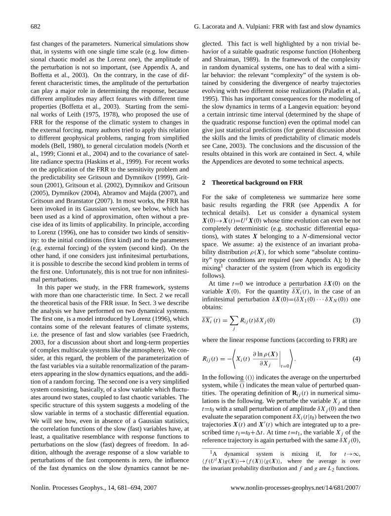
Fig. 9. DW model withε = 1: time signal sample of the slow variableq0(t). The ratio between fast and slow

characteristic times isε ∼ 0.1 (see text).

31

Fig. 9. DW model withε=1: time signal sample of the slow vari-ableq0(t). The ratio between fast and slow characteristic times isε∼0.1 (see text).

slow variablex=q0:

dx

dt= −

∂V

∂x= 2

√Hx − x3

with

V (x) = H −√Hx2

+1

4x4 (21)

The system (21) has one unstable steady state inx0=0 cor-responding to the top of the hill of heightH , and two stablesteady states inx1/2=±(4H)1/4, i.e. the bottom of the val-leys. The presence of the coupling (c 6=0) between slow andfast variables can induce transitions between the two valleys.The parameters in Eqs. (17), (18), (19), and (20) are fixedto the following values:σL=10, rL=28, bL=8/3, i.e. theclassical set-up corresponding to the chaotic regime for theLorenz-63 system;H=4, the height of the barrier;c=0.5,the coupling constant that rules the transition time scale ofq0(t) between the two valleys; by settingε=1, the ratioε be-tween fast and slow characteristic times, see Eqs. (7) and (8),isO(10−1).

Since the time scale of theq0(t) well-to-well transitionsmay be considerably longer, depending on 1/c, than the char-acteristic time ofq1(t), of orderO(1), we refer toq0 as theslow variable, or the low-frequency observable, and toq1 asthe fast variable, or the high-frequency forcing, of the deter-ministic DW model. It can be easily shown that, forc=0,small perturbations1q0 around the two potential minimaat ±(4H)1/4 relax exponentially to zero with characteristictime 1/4

√H . For sufficiently large values ofc, the climatic

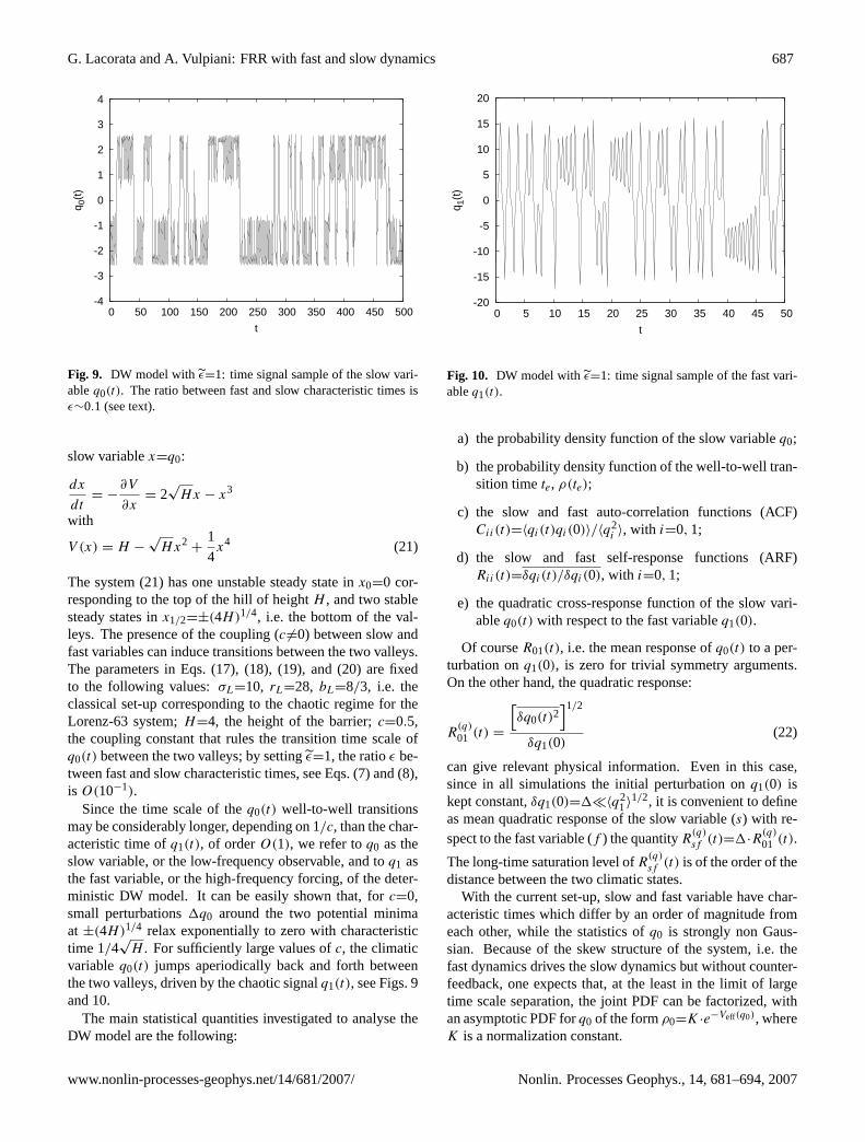
variableq0(t) jumps aperiodically back and forth betweenthe two valleys, driven by the chaotic signalq1(t), see Figs.9and10.

The main statistical quantities investigated to analyse theDW model are the following:

-20

-15

-10

-5

0

5

10

15

20

0 5 10 15 20 25 30 35 40 45 50

q 1(t

)

t

Fig. 10. DW model withε = 1: time signal sample of the fast variableq1(t).

32

Fig. 10. DW model withε=1: time signal sample of the fast vari-ableq1(t).

a) the probability density function of the slow variableq0;

b) the probability density function of the well-to-well tran-sition timete, ρ(te);

c) the slow and fast auto-correlation functions (ACF)Cii(t)=〈qi(t)qi(0)〉/〈q2

i 〉, with i=0,1;

d) the slow and fast self-response functions (ARF)Rii(t)=δqi(t)/δqi(0), with i=0,1;

e) the quadratic cross-response function of the slow vari-ableq0(t) with respect to the fast variableq1(0).

Of courseR01(t), i.e. the mean response ofq0(t) to a per-turbation onq1(0), is zero for trivial symmetry arguments.On the other hand, the quadratic response:

R(q)

01 (t) =

[δq0(t)2

]1/2

δq1(0)(22)

can give relevant physical information. Even in this case,since in all simulations the initial perturbation onq1(0) iskept constant,δq1(0)=1�〈q2

1〉1/2, it is convenient to define

as mean quadratic response of the slow variable (s) with re-spect to the fast variable (f ) the quantityR(q)sf (t)=1·R

(q)

01 (t).

The long-time saturation level ofR(q)sf (t) is of the order of thedistance between the two climatic states.

With the current set-up, slow and fast variable have char-acteristic times which differ by an order of magnitude fromeach other, while the statistics ofq0 is strongly non Gaus-sian. Because of the skew structure of the system, i.e. thefast dynamics drives the slow dynamics but without counter-feedback, one expects that, at the least in the limit of largetime scale separation, the joint PDF can be factorized, withan asymptotic PDF forq0 of the formρ0=K ·e−Veff(q0), whereK is a normalization constant.



-0.2

0

0.2

0.4

0.6

0.8

1

0 0.2 0.4 0.6 0.8 1 1.2 1.4 1.6 1.8 2

R11

(t),

C11

(t)

t

Fig. 11. DW model with ε = 1: autocorrelationC11(t) (full line) and self-responseR11(t), with statistical

error bars, for the fast variableq1.

33

Fig. 11. DW model with ε=1: autocorrelationC11(t) (full line)and self-responseR11(t), with statistical error bars, for the fast vari-ableq1.

-0.2

0

0.2

0.4

0.6

0.8

1

0 2 4 6 8 10 12 14 16 18 20

R00

(t),

C00

(t)

t

Fig. 12. DW model with ε = 1: AutocorrelationC00(t) (full line) and self-responseR00(t), with statistical

error bars, for the slow variableq0.

34

Fig. 12. DW model with ε=1: AutocorrelationC00(t) (full line)and self-responseR00(t), with statistical error bars, for the slowvariableq0.

The FR properties of the deterministic DW model, for thefast and slow variables, are shown in Figs.11and12, respec-tively.

The slow self-responseR00(t) initially decreases exponen-tially with characteristic time 1/4

√H (H=4), i.e. the same

behavior of the relaxation of a small perturbation near thebottom of a valley forc=0. Then,R00(t) relaxes to zeromuch more slowly. It is natural to assume that this is due tothe long-time jumps between the valleys. It is well evidentthatR00 behaves rather differently fromC00, whileR11 andC11 have, at least, the same qualitative shape. On the otherhand, the autocorrelation (self-response) time scales of thetwo variables differ from each other of a factor∼10, compat-ibly with the fact that the ratio between fast and slow charac-teristic times isε∼0.1, for the current set-up (ε=1).

-0.2

0

0.2

0.4

0.6

0.8

1

0 5 10 15 20

R00

(t),

C00

(t),

C(t

)

t

Fig. 13. DW model with ε = 0.01, implying ε ∼ 10−3: autocorrelationC00(t) (dashed line), self-response

R00(t), with statistical error bars, and the correlation functionC(t) predicted by the FRR (full line) which is

actually undistinguishable from the response.

35

Fig. 13. DW model withε=0.01, implyingε∼10−3: autocorrela-tionC00(t) (dashed line), self-responseR00(t), with statistical errorbars, and the correlation functionC(t) predicted by the FRR (fullline) which is actually undistinguishable from the response.

Since the statistics is far from being Gaussian, the “cor-rect” correlation function which satisfies the FR theorem, forthe slow variable, has the form:

C(t) = −

⟨q0(t)

∂ρε(q0, q1, q2, q3)

∂q0

∣∣∣∣t=0

⟩(23)

whereρε(q0, q1, q2, q3) is the (unknown) joint PDF of thestate variable of the system at a fixedε. In the limit of largetime separation, i.e. forε→0, one expects that the asymptoticPDFρ0(q0, q1, q2, q3) is factorized:

ρ0(q0, q1, q2, q3) = Ke−Veff(q0)ρL(q1, q2, q3) (24)

whereK is a normalization constant, andρL is the PDF ofthe Lorenz-63 state variable. Under this condition, the rightcorrelation function predicted by the FRR has a relativelysimple form:

C(t) =

⟨q0(t)

∂Veff(q0)

∂q0

∣∣∣∣t=0

⟩(25)

whereVeff indicates the effective potential. Forε∼10−1 (cor-responding toε=1) we have checked numerically that thejoint PDF is not yet factorized, while for a very small ra-tio between the characteristic times,ε∼10−3 (correspondingto ε=10−2), the form (24) holds and, takingVeff ∝ V , weobtain a very good agreement betweenR00(t) andC(t), seeFig. 13.

The cross-response properties of the DW model, measuredby the quantityR(q)sf (t), are reported in Fig.18. We willconsider again later this issue when discussing the stochas-tic modeling. While the mean (slow-to-fast) cross-responseis null (not shown), its fluctuations grow with time. Thismeans that an initial uncertainty on the fast variables has con-sequences for the predictability of the slow variable, since it



0.0001

0.001

0.01

0.1

0 10 20 30 40 50 60 70

ρ(t e

)

te

Fig. 14. Comparison of the PDFs of the transition timete between the two climatic states for the DW model

(full line) and the WNDW model (dashed line), forε = 1 (ε ∼ 0.1).

36

Fig. 14. Comparison of the PDFs of the transition timete betweenthe two climatic states for the DW model (full line) and the WNDWmodel (dashed line), forε=1 (ε∼0.1).

induces a mean separation growth between two initially close“climatic” states of theq0 variable. At small times,R(q)sf (t)grows exponentially in time, i.e. it is driven by the chaoticcharacter of the fast variable while, at very long times, thewell-to-well aperiodic jumps play the dominant role and thegrowth speed eventually decreases to zero until saturationsets in.

Let us now consider a stochastic model for the slow vari-ableq0(t), obtained by replacing the fast variableq1, in theequation forq0, with a white noise. One has a Langevinequation of the kind:

dq0

dt(t) = 2

√Hq0(t)− q3

0 + σ · ξ(t) (26)

where ξ(t) is a Gaussian process with〈ξ(t)〉=0 and〈ξ(t)ξ(t ′)〉=δ(t−t ′). We call Eq. (26) the WNDW model.The valueσ=19.75 is determined by requiring that the PDFsof the well-to-well transition times have the same asymptoticbehavior (i.e. exponential tail with the same exponent), seeFig. 14.

Let us notice that, in this case, because of the skew struc-ture of the original system, the stochastic modeling is (rel-atively) simple and, differently from the generic case, thenoise is additive. The time signalq0(t) obtained from theWNWD model is reported in Fig.15. One observes strongsimilarities in the long-time transition statistics with respectto the deterministic model, even though the PDFs of the slowvariable are quite different from one another, see Fig.16.

The FR properties of the WNDW model are reportedin Fig. 17. The slow variable is distributed according to∼e−V (q0)/K , with K=σ 2/2, and the FR theorem predictionis verified, i.e. one has a good agreement betweenR00(t) andthe correlation functionC(t).

-4

-3

-2

-1

0

1

2

3

4

0 50 100 150 200 250 300 350 400 450 500

q 0(t

)

t

Fig. 15. WNDW model: time signal sample of the slow variableq0(t).

37

Fig. 15. WNDW model: time signal sample of the slow variableq0(t).

0

0.1

0.2

0.3

0.4

0.5

0.6

0.7

-3 -2 -1 0 1 2 3

ρ(q 0

)

q0

Fig. 16. PDFs of the slow variableq0 for the DW model withε = 1, i.e. ε ∼ 0.1 (full line), the WNDW model

(dashed line) and the DW model withε = 10−2, i.e. ε ∼ 10−3 (dotted line). In the limitε → 0, the PDFs of

the deterministic model and of the stochastic model collapse.

38

Fig. 16. PDFs of the slow variableq0 for the DW model withε=1,i.e. ε∼0.1 (full line), the WNDW model (dashed line) and the DWmodel with ε=10−2, i.e. ε∼10−3 (dotted line). In the limitε→0,the PDFs of the deterministic model and of the stochastic modelcollapse.

We redefine, as already seen when discussing the stochas-tic model approximating the Lorenz-96 system, the quadraticcross-response functionR(q)sf (t) as the root mean squaregrowth of the errorδq0(t) induced by two different noise re-alizations.

In Fig. 18, the behavior ofR(q)sf (t) for the deterministicDW system and its stochastic model is reported. The WNDWmodel is not able to reproduce the two-time behavior of thedeterministic model, mainly due to the impossibility to con-trol the amplitude of the initial perturbation. Because of that,the error on the climatic state of the system saturate veryquickly, as soon as the trajectory starts jumping between thewells.



-0.2

0

0.2

0.4

0.6

0.8

1

0 2 4 6 8 10 12 14 16 18 20

R00

(t),

C00

(t)

, C

(t)

t

Fig. 17. WNDW model: autocorrelationC00(t) (dashed line), self-responseR00(t), with statistical error bars,

and the correlation functionC(t) predicted by the FRR (full line).

39

Fig. 17. WNDW model: autocorrelationC00(t) (dashed line), self-responseR00(t), with statistical error bars, and the correlation func-tionC(t) predicted by the FRR (full line).

4 Discussion and conclusive remarks

In this paper we have presented a detailed investigation of theFluctuation-Response properties of chaotic systems with fastand slow dynamics. The numerical study has been performedon two models, namely the 360-variable Lorenz-96 system,with reciprocal feedback between fast and slow variables,and a simplified low dimensional system, both of which areable to capture the main features, and related difficulties, typ-ical of the multiscale systems. The first point we wish toemphasize is how, even in non Hamiltonian systems, a gen-eralized Fluctuation-Response Relation (FRR) holds. Thisallows for a link between the average relaxation of pertur-bations and the statistical properties (correlation functions)of the unperturbed system. Although one has non Gaus-sian statistics, the correlation functions of the slow (fast)variables have at least a qualitative resemblance with the re-sponse functions to perturbations on the slow (fast) degreesof freedom. The average response function of a slow variableto perturbations of the fast degrees of freedom is zero, never-theless the impact of the fast dynamics on the slowly varyingcomponents cannot be neglected. This fact is clearly high-lighted by the behavior of a suitable quadratic response func-tion. Such a phenomenon, which can be regarded as a sortof sensitivity of the slow variables to variations of the fastcomponents, has an important consequence for the modelingof the slow dynamics in terms of a Langevin equation. Evenan optimal model (i.e. able to mimic autocorrelation and self-response of the slow variable), beyond a certain intrinsic timeinterval, can give just statistical predictions, in the sense that,at most, one can hope to have an agreement among the statis-tical features of system and model. In stochastic dynamicalsystems, one has to deal with a similar behavior: the relevant“complexity” of the systems is obtained by considering the

0.0001

0.001

0.01

0.1

1

10

0 1 2 3 4 5 6 7 8 9 10

Rsf

(q) (t

)

t

Fig. 18.Quadratic cross-response functionR(q)sf (t) for the DW model (full line) and the WNDW model (dashed

line). The growth rates ofR(q)sf (t) for the DW model are compatible with the two characteristic times of the

system, while for the WNDW modelR(q)sf (t) quickly saturates in a very short time.

40

Fig. 18. Quadratic cross-response functionR(q)sf(t) for the DW

model (full line) and the WNDW model (dashed line). The growth

rates ofR(q)sf(t) for the DW model are compatible with the two char-

acteristic times of the system, while for the WNDW modelR(q)sf(t)

quickly saturates in a very short time.

divergence of nearby trajectories evolving under two differ-ent noise realizations. Therefore a good model for the slowdynamics (e.g. a Langevin equation) must show a sensitivityto the noise.

Appendix A

Generalized FRR

In this Appendix we give a derivation, under general ratherhypothesis, of a generalized FRR. Consider a dynamical sys-tem x(0)→x(t)=U tx(0) with statesx belonging to aN -dimensional vector space. For the sake of generality, wewill consider the case in which the time evolution can alsobe not completely deterministic (e.g. stochastic differentialequations). We assume the existence of an invariant proba-bility distributionρ(x), for which some “absolute continuity”type conditions are required (see later), and the mixing char-acter of the system (from which its ergodicity follows). Notethat no assumption is made onN .

Our aim is to express the average response of a genericobservableA to a perturbation, in terms of suitable correla-tion functions, computed according to the invariant measureof the unperturbed system. At the first step we study thebehavior of one component ofx, sayxi , when the system,described byρ(x), is subjected to an initial (non-random)perturbation such thatx(0)→x(0)+1x0. This instantaneouskick3 modifies the density of the system intoρ′(x), related to

3The study of an “impulsive” perturbation is not a severe limita-tion, e.g. in the linear regime from the (differential) linear response



the invariant distribution byρ′(x)=ρ(x−1x0). We introducethe probability of transition fromx0 at time 0 tox at timet , W(x0,0→x, t). For a deterministic system, with evolu-tion lawx(t)=U tx(0), the probability of transition reduces toW(x0,0→x, t)=δ(x−U tx0), whereδ(·) is the Dirac’s delta.Then we can write an expression for the mean value of thevariablexi , computed with the density of the perturbed sys-tem:⟨xi(t)

⟩′=

∫ ∫xiρ

′(x0)W(x0,0 → x, t) dx dx0 . (A1)

The mean value ofxi during the unperturbed evolution canbe written in a similar way:⟨xi(t)

⟩=

∫ ∫xiρ(x0)W(x0,0 → x, t) dx dx0 . (A2)

Therefore, definingδxi=〈xi〉′−〈xi〉, we have:

δxi (t) =

∫ ∫xi F(x0,1x0) ρ(x0)W(x0,0 → x, t) dx dx0

=

⟨xi(t) F (x0,1x0)

⟩(A3)

where

F(x0,1x0) =

[ρ(x0 −1x0)− ρ(x0)

ρ(x0)

]. (A4)

Let us note here that the mixing property of the system is re-quired so that the decay to zero of the time-correlation func-tions assures the switching off of the deviations from equi-librium.

For an infinitesimal perturbationδx(0) = (δx1(0) · · · δxN(0)), if ρ(x) is non-vanishing and differentiable, the functionin Eq. (A4) can be expanded to first order and one obtains:

δxi (t) = −

∑j

⟨xi(t)

∂ ln ρ(x)∂xj

∣∣∣∣t=0

⟩δxj (0)

≡

∑j

Rij (t)δxj (0) (A5)

which defines the linear response

Rij (t) = −

⟨xi(t)

∂ ln ρ(x)∂xj

∣∣∣∣t=0

⟩(A6)

of the variablexi with respect to a perturbation ofxj . Onecan easily repeat the computation for a generic observableA(x):

δA (t) = −

∑j

⟨A(x(t))

∂ ln ρ(x)∂xj

∣∣∣∣t=0

⟩δxj (0) . (A7)

For Langevin equations, the differentiability ofρ(X) iswell established. On the contrary, one could argue that in a

one understands the effect of a generic perturbation.

chaotic deterministic dissipative system the above machin-ery cannot be applied, because the invariant measure is notsmooth at all. Typically the invariant measure of a chaotic at-tractor has a multifractal character and its Renyi dimensionsdq are not constant (Paladin and Vulpiani, 1987). In chaoticdissipative systems the invariant measure is singular, how-ever the previous derivation of the FRR is still valid if oneconsiders perturbations along the expanding directions. Fora mathematically oriented presentation see Ruelle (1998). Ageneral response function has two contributions, correspond-ing respectively to the expanding (unstable) and the contract-ing (stable) directions of the dynamics. The first contributioncan be associated to some correlation function of the dynam-ics on the attractor (i.e. the unperturbed system). On the con-trary this is not true for the second contribution (from thecontracting directions), this part to the response is very dif-ficult to extract numerically (Cessac and Sepulchre, 2007).In chaotic deterministic systems, in order to have a differ-entiable invariant measure, one has to invoke the stochasticregularization (Zeeman, 1990). If such a method is not feasi-ble, one can use the direct approach by Abramov and Majda(2007). For a study of the FRR in chaotic atmospheric sys-tems, see Dymnikov and Gritsoun (2005) and Gritsoun andBranstator (2007).

Let us notice that a small amount of noise, that is alwayspresent in a physical system, smoothen theρ(x) and the FRRcan be derived. We recall that this “beneficial” noise hasthe important role of selecting the natural measure, and, inthe numerical experiments, it is provided by the round-offerrors of the computer. We stress that the assumption on thesmoothness of the invariant measure allows to avoid subtletechnical difficulties.

Appendix B

A general remark on the decay of correlationfunctions

Using some general arguments one has that all the (typical)correlation functions at large time delay have to relax to zerowith the same characteristic time, related to spectral proper-ties of the operatorL which rules the time evolution of theP(X, t):

∂

∂tP (X, t) = LP(X, t) . (B1)

In the case of ordinary differential equations

dXi/dt = Qi(X) i = 1, · · · , N (B2)

the operatorL has the shape

LP(X, t) = −

∑i

∂

∂Xi

(Qi(X)P (X, t)

). (B3)



For Langevin equations i.e. in Eq. (B2) Qi is replaced byQi+ηi where{ηi} are Gaussian processes with<ηi(t)>=0and<ηi(t)ηj (t ′)>=23i,j δ(t − t ′), one has

LP(X, t) = −∑i∂∂Xi

(Qi(X)P (X, t)

)+

∑ab3i,j

∂2

∂Xi∂XiP(X, t) .

(B4)

Let us introduce the eigenvalues{αk} and the eigenfunc-tions{ψk} of L:

Lψk = αkψk . (B5)

Of courseψ0=Pinv andα0=0, and typically in mixing sys-temsRe αk<0 for k=1,2, .... Furthermore assuming that co-efficient{g1, g2, ...} and{h1, h2, ...} exist such that functionsg(X) andh(X) are uniquely expanded as

g(X) =

∑k=0

gkψk(X) , h(X) =

∑k=0

hkψk(X) , (B6)

so we have

Cg,f (t) =

∑k=1

gkhk < ψ2k > eαk t , (B7)

where Cg,f (t)=<g(X(t))h(X(t))>−<g(X)><h(X)>.For “generic” functionsg and f , i.e. if they are not or-thogonal toψ1 so thatg1 6=0 andh1 6=0, at large time thecorrelationCg,f (t) approaches to zero as

Cg,f (t) ∼ e−t/τc , τc =1

|Re α1|. (B8)

In some cases, e.g. very intermittent systems like theLorenz model atr'166.07,Re α1=0 so the decay is not ex-ponentially fast.

Appendix C

Lyapunov exponent in dynamical systems with noise

In systems with noise, the simplest way to introduce theLyapunov exponent is to treat the random term as a time-dependent term. Basically one considers the separation oftwo close trajectories with the same realization of noise.Only for sake of simplicity consider a one-dimensionalLangevin equation

dx

dt= −

∂V (x)

∂x+ σ η , (C1)

whereη(t) is a white noise andV (x) diverges for| x | →∞,like, e.g., the usual double well potentialV=−x2/2+x4/4.

The Lyapunov exponentλσ , associated with the separationrate of two nearby trajectories with the same realization ofη(t), is defined as

λσ = limt→∞

1

tln |z(t)| (C2)

where the evolution of the tangent vector is given by:

dz

dt= −

∂2V (x(t))

∂x2z(t). (C3)

The quantityλσ obtained in the previous way, although welldefined, i.e. the Oseledec theorem (Bohr et al., 1998) holds,it is not always a useful characterization of complexity.

Since the system is ergodic with invariant probability dis-tribution P(x)=C1e

−V (x)/C2, whereC1 is a normalizationconstant andC2=σ

2/2, one has:

λσ = limt→∞1t

ln |z(t)|

= − limt→∞1t

∫ t0 ∂

2xxV (x(t

′))dt ′

= −C1∫∂2xxV (x)e

−V (x)/C2 dx

= −C1C2

∫(∂xV (x))

2e−V (x)/C2 dx < 0 .

(C4)

This has a rather intuitive meaning: the trajectoryx(t) spendsmost of the time in one of the “valleys” where−∂2

xxV (x)<0and only short intervals on the “hills” where−∂2

xxV (x)>0,so that the distance between two trajectories evolving withthe same noise realization decreases on average. The previ-ous result for the 1-D Langevin equation can easily be gen-eralized to any dimension for gradient systems if the noise issmall enough (Loreto et al., 1996).

A negative value ofλσ implies a fully predictable processonly if the realization of the noise is known. In the case oftwo initially close trajectories evolving under two differentnoise realizations, after a certain timeTσ , the two trajecto-ries can be very distant, because they can be in two differentvalleys. Forσ→0, due to the Kramers formula (Gardiner,1990), one hasTσ∼e1V/σ

2, where1V is the difference be-

tween the values ofV on the top of the hill and at the bottomof the valley.

Let us now discuss the main difficulties in defining the no-tion of “complexity” of an evolution law with a random per-turbation, discussing a simple case. Consider the 1-D map

x(t + 1) = f [x(t), t] + σw(t), (C5)

wheret is an integer andw(t) is an uncorrelated random pro-cess, e.g.w are independent random variables uniformly dis-tributed in[−1/2,1/2]. For the largest LEλσ , as defined in(C2), now one has to study the equation

z(t + 1) = f ′[x(t), t] z(t), (C6)

wheref ′=df/dx.

Following the approach in (Paladin et al., 1995) letx(t) bethe trajectory starting atx(0) andx′(t) be the trajectory start-ing fromx′(0)=x(0)+δx(0). Letδ0≡|δx(0)| and indicate byτ1 the minimum time such that|x′(τ1)−x(τ1)|≥1. Then, weput x′(τ1)=x(τ1)+δx(0) and defineτ2 as the time such that|x′(τ1+τ2)−x(τ1+τ2)|>1 for the first time, and so on. Inthis way the Lyapunov exponent can be defined as

λ =1

τln

(1

δ0

)(C7)



being τ=∑τi/N whereN is the number of the intervals

in the sequence. If the above procedure is applied by con-sidering the same noise realization for both trajectories,λ inEq. (C2) coincides withλσ (if λσ>0). Differently, by con-sidering two different realizations of the noise for the twotrajectories, we have a new quantity

Kσ =1

τln

(1

δ0

), (C8)

which naturally arises in the framework of information the-ory and algorithmic complexity theory: note thatKσ / ln 2 isthe number of bits per unit time one has to specify in order totransmit the sequence with a precisionδ0, The generalizationof the above treatment toN -dimensional maps or to ordinarydifferential equations is straightforward.

If the fluctuations of the effective Lyapunov expo-nent γ (t) (in the case of Eq.C5 γ (t) is nothing butln |f ′(x(t))|) are very small (i.e. weak intermittency) one hasKσ=λ+O(σ/1).

The interesting situation happens for strong intermittencywhen there are alternations of positive and negativeγ duringlong time intervals: this induces a dramatic change for thevalue ofKσ . Numerical results on intermittent maps (Pal-adin et al., 1995) show that the same system can be regardedeither as regular (i.e.λσ<0), when the same noise realiza-tion is considered for two nearby trajectories, or as chaotic(i.e.Kσ>0), when two different noise realizations are con-sidered. We can say that a negativeλσ for some value ofσ in not an indication that “noise induces order”; a correctconclusion is that noise can induce synchronization.

Acknowledgements.We warmly thank A. Mazzino, S. Musacchio,R. Pasmanter and A. Puglisi for interesting discussions andsuggestions, and two anonymous referees for their contructivecriticism in reviewing this paper.

Edited by: O. TalagrandReviewed by: two anonymous referees

References

Abramov, R. and Majda, A.: New approximations and tests of lin-ear fluctuation-response for chaotic nonlinear forced-dissipativedynamical systems, J. Nonlinear Sci., accepted, 2007.

Bell, T. L.: Climate sensitivity from fluctuation-dissipation: somesimple model tests, J. Atmos. Sci., 37, 1700–1707, 1980.

Biferale, L., Daumont, I., Lacorata, G., and Vulpiani, A.:Fluctuation-response relation in turbulent systems, Phys. Rev. E,65, 016302, 016302-1–016302-7, 2002.

Boffetta, G., Lacorata, G., Musacchio, S., and Vulpiani, A.: Relax-ation of finite perturbations: Beyond the Fluctuation-Responserelation, Chaos, 13, 806–811, 2003.

Bohr, T., Jensen, M. H., Paladin, G., and Vulpiani, A.: Dynami-cal systems approach to turbulence, Cambridge University Press,UK, 1998.

Cane, M.: Understanding and predicting the world’s climate sys-tem, Chaos in geophysical flows, Chaos in geophysical flows,edited by: Boffetta, G., Lacorata, G., Visconti, G., and Vulpiani,A., Otto Eds., Torino, Italy, 2003.

Cessac, B. and Sepulchre, J.-A.: Linear response, susceptibility andresonance in chaotic toy models, Physica D, 225, 13–28, 2007.

Cionni, I., Visconti, G., and Sassi, F.: Fluctuation-dissipation the-orem in a general circulation model, Geophys. Res. Lett., 31,L09206, doi:10.1029/2004GL019739, 2004.

Deker, U. and Haake, F.: Fluctuation-dissipation theorems for clas-sical processes, Phys. Rev. A, 11, 2043–2056, 1975.

Ditlevsen, P. D.: Observation ofα-stable noise induced millennialclimate changes from an ice-core record, Geophys. Res. Lett.,26(10), 1441–1444, 1999.

Dymnikov, V. P.: Potential Predictability of Large-Scale Atmo-spheric Processes, Izvestiya, Atmospheric and Oceanic Physics,40(5), 513–519, 2004.

Dymnikov, V. P. and Gritsoun, A. S.: Climate model attractors:chaos, quasi-regularity and sensitivity to small perturbations ofexternal forcing, Nonlin. Processes Geophys., 8, 201–209, 2001,http://www.nonlin-processes-geophys.net/8/201/2001/.

Dymnikov, V. P. and Gritsoun, A. S.: Current problems in the math-ematical theory of climate, Izvestiya, Atmospheric and OceanicPhysics, 41, 294–314, 2005.

Falcioni, M., Isola, S., and Vulpiani, A.: Correlation functions andrelaxation properties in chaotic dynamics and statistical mechan-ics, Phys. Lett. A, 144, 341–346, 1990.

Fraedrich, K.: Predictability: short and long-term memory of theatmosphere, Chaos in geophysical flows, Chaos in geophysicalflows, edited by: Boffetta, G., Lacorata, G., Visconti, G., andVulpiani, A., Otto Eds., Torino, Italy, 2003.

Frisch, U.: Turbulence, Cambridge University Press, UK, 1995.Gardiner, C. W.: Handbook of stochastic methods for Physics,

Chemistry and the Natural Sciences, Springer-Verlag, Berlin,Germany, 1990.

Givon, D., Kupferman, R., and Stuart, A.: Extracting macroscopicdynamics: model problems and algorithms, Nonlinearity, 17, 55–127, 2004.

Gritsoun, A. S.: Fluctuation-dissipation theorem on attractors ofatmospheric models, Russ. J. Numer. Analysis Math. Modelling,16, 115–133, 2001.

Gritsoun, A. S. and Branstator, G.: Climate Response Using aThree-Dimensional Operator Based on the Fluctuation Dissipa-tion Theorem, J. Atmos. Sci., 64(7), 2558-2575, 2007.

Gritsoun, A. S., Branstator, G., and Dymnikov, V. P.: Constructionof the linear response operator of an atmospheric general circu-lation model to small external forcing, Russ. J. Numer. AnalysisMath. Modelling, 17, 399–416, 2002.

Gritsoun, A. S. and Dymnikov, V. P.: Barotropic atmosphere re-sponse to small external action: theory and numerical experi-ments, Izvestiya, Atmospheric and Oceanic Physics, 35, 511–525, 1999.

Haskins, R., Goody, R., and Chen, L.: Radiance covariance andclimate models, J. Climate, 12, 1409–1422, 1999.

Hohenberg, P. C. and Shraiman, B. I.: Chaotic behavior of an ex-tended system, Physica D, 37, 109–115, 1989.

Imkeller, P. and von Storch, J.-S. (Eds.): Stochastic Climate Mod-els, Birkhauser, Basel, Switzerland, 2001.

Kraichnan, R. H.: Classical fluctuation-relaxation theorem, Phys.


http://www.nonlin-processes-geophys.net/8/201/2001/


Rev., 113, 1181–1182, 1959.Kraichnan, R. H.: Deviations from fluctuation-relaxation relations,

Physica A, 279, 30–36, 2000.Kraichnan, R. H. and Montgomery, D.: Two-dimensional turbu-

lence, Rep. Prog. Phys., 43, 547–619, 1980.Kubo, R.: The fluctuation-dissipation theorem, Rep. Prog. Phys.,

29, 255–284, 1966.Kubo, R.: Brownian motion and nonequilibrium statistical mechan-

ics, Science, 233, 330–334, 1986.Leith, C. E.: Climate response and fluctuation-dissipation, J. At-

mos. Sci., 32, 2022–2026, 1975.Leith, C. E.: Predictability of climate, Nature, 276, 352–355, 1978.Lorenz, E. N.: Deterministic nonperiodic flow, J. Atmos. Sci., 20,

130–141, 1963.Lorenz, E. N.: Predictability – a problem partly solved, Proceed-

ings, Seminar on Predictability ECMWF, 1, 1–18, 1996.Loreto, V., Paladin, G., and Vulpiani, A.: On the concept of com-

plexity for random dynamical systems, Phys. Rev. E, 53, 2087–2098, 1996.

Majda, A. J., Abramov, R., and Grote, M.: Information theory andstochastics for multiscale nonlinear systems, CRM monographseries 25, American Mathematical Society, 2005.

Majda, A. J. and Franzke, C.: Low Order Stochastic Mode Reduc-tion for a Prototype Atmospheric GCM, J. Atmos. Sci., 63(2),457-479, 2006.

Majda, A. J., Timofeyev, I., and Vanden-Eijnden, E.: Models forstochastic climate prediction, Proc. Natl. Acad. Sci. USA, 96,14 687–14 691, 1999.

Majda, A. J., Timofeyev, I., and Vanden-Eijnden, E.: A mathe-matical framework for stochastic climate models, Commun. PureAppl. Math., 54, 891–974, 2001.

Majda, A. J. and Wang, X.: Nonlinear Dynamics and StatisticalTheories for Basic Geophysical Flows, Cambridge UniversityPress, UK, 2006.

Marwan, N., Trauth, M., Vuille, M., and Kurths, J.: Comparingmodern and Pleistocene ENSO-like influences in NW Argentinausing nonlinear time series analysis methods, Clim. Dynam., 21,317–326, 2003.

Matsumoto, K. and Tsuda, I.: Noise-induced order, J. Stat. Phys.,31, 87–106, 1983.

Mazzino, A., Musacchio, S., and Vulpiani, A.: Multiple scale analy-sis and renormalization for preasymptotic scalar transport, Phys.Rev. E, 71, 011113, 1–11, 2005.

McComb, W. D. and Kiyani, K.: Eulerian spectral closures forisotropic turbulence using a time-ordered fluctuation-dissipationrelation, Phys. Rev. E, 72, 016309, 016309-1–016309-12, 2005.

Moeng, C.-H.: A Large-Eddy Simulation model for the study ofplanetary boundary layer turbulence, J. Atmos. Sci., 41, 2052–2062, 1984.

Moeng, C.-H. and Sullivan, P. P.: A comparison of shear and buoy-ancy driven planetary boundary layer flows, J. Atmos. Sci., 51,999–1021, 1994.

North, G. R., Bell, R. E., and Hardin, J. W.: Fluctuation dissipationin a general circulation model, Clim. Dynam., 8, 259–264, 1993.

Paladin, G., Serva, M., and Vulpiani, A.: Complexity in dynamicalsystems with noise, Phys. Rev. Lett., 74, 66–69, 1995.

Paladin, G. and Vulpiani, A.: Anomalous scaling laws in multifrac-tal objects, Phys. Rep., 156, 147–225, 1987.

Pasmanter, R. A.: On long-lived vortices in 2-D viscous flows,most probable states of inviscid 2-D flows and a soliton equa-tion, Phys. Fluids, 6, 1236–1241, 1994.

Pikovsky, A., Rosenblum, M., and Kurths, J.: Synchronization: auniversal concept in nonlinear sciences, Cambridge UniversityPress, UK, 2003.

Rose, R. H. and Sulem, P. L.: Fully developed turbulence and sta-tistical mechanics, J. Phys., 39, 441–484, 1978.

Ruelle, D.: General linear response formula in statistical mechan-ics, and the fluctuation-dissipation theorem far from equilibrium,Phys. Lett. A, 245, 220–224, 1998.

Sullivan, P. P., McWilliams, J.-C., and Moeng, C.-H.: A subgrid-scale model for large-eddy simulation of planetary boundarylayer flows, Bound. Layer Meteorol., 71, 247–276, 1994.

Zeeman, E. C.: Stability of dynamical systems, Nonlinearity, 1,115–135, 1988.


fluctuation-response relation and modeling in systems ... - le.isac.cnr.it · g. lacorata and a....

Documents