fluid flow investigation through small turbodrill for

Mechanical Engineering Research; Vol. 3, No. 1; 2013 ISSN 1927-0607 E-ISSN 1927-0615

Published by Canadian Center of Science and Education

1

Fluid Flow Investigation through Small Turbodrill for Optimal Performance

Amir Mokaramian1, Vamegh Rasouli1 & Gary Cavanough2 1 Deep Exploration Technologies Cooperative Research Centre (DET CRC), and Department of Petroleum Engineering, Curtin University, Australia 2 Research Programme Leader, Deep Exploration Technologies Cooperative Research Centre (DET CRC), and CSIRO, Queensland Centre for Advanced Technologies (QCAT), Australia

Correspondence: Amir Mokaramian, Department of Petroleum Engineering, Curtin University, ARRC building, Kensington, Western Australia 6151. Tel: 61-89-266-4994. E-mail: [email protected]

Received: November 29, 2012 Accepted: December 27, 2012 Online Published: January 20, 2013

doi:10.5539/mer.v3n1p1 URL: http://dx.doi.org/10.5539/mer.v3n1p1

Abstract

Basic design methodology for a new small multistage Turbodrill (turbine down hole motor) optimized for small size Coiled Tube (CT) Turbodrilling system for deep hard rocks mineral exploration drilling is presented. Turbodrill is a type of axial turbomachinery which has multistage of stators and rotors. It converts the hydraulic power provided by the drilling fluid (pumped from surface) to mechanical power through turbine motor. For the first time, new small diameter (5-6 cm OD) water Turbodrill with high optimum rotation speed of higher than 2,000 revolutions per minute (rpm) were designed through comprehensive numerical simulation analyses. The results of numerical simulations (Computational Fluid Dynamics (CFD)) for turbodrill stage performance analysis with asymmetric blade’s profiles on stator and rotor, with different flow rates and rotation speeds are reported. This follows by Fluid-Structural Interaction (FSI) analyses for this small size turbodrill in which the finite element analyses of the stresses are performed based on the pressure distributions calculated from the CFD modeling. As a result, based on the sensitivity analysis, optimum operational and design parameters are proposed for gaining the required rotation speed and torque for hard rocks drilling.

Keywords: hydraulic turbodrill, turbine down hole motor, turbodrill design and performance, Coiled Tube (CT) drilling, Computational Fluid Dynamics (CFD), numerical simulation

1. Introducation

Coiled Tube (CT) Turbodrilling technology has been recently proposed for drilling deep hard rocks for mineral exploration applications (Mokaramian et al., 2012). Coiled Tube (CT) is a continuous length of ductile steel or carbon fiber tube that is stored and transported over a large reel (see Figure 1). The CT Unit (CTU) consists of four basic elements: 1) Reel, for storage and transport of the CT, 2) Injector Head, to provide the surface drive force to run and retrieve the CT, 3) Control Cabin, from which the equipment operator monitors and controls the CT, and 4) Power Pack, to generate hydraulic and pneumatic power required to operate the CT unit. In mineral exploration, drilling small size holes as fast as possible and obtaining reliable rock samples to the surface yields several advantages over conventional drilling methods. Coiled tube (CT) allows fast drilling by eliminating the connection time and providing continuous circulation during drilling. This enables quick access to the zone of interest to collect the powder size cuttings or obtain core samples.

Coiled tube itself cannot rotate and therefore a down hole motor is needed to provide mechanical power and rotation to the bit. There are many special design criteria to be considered for successful operation of down hole motors in CT drilling (RIO, 2004; IT, 2007). One major concern is that it is often difficult to produce enough weight on bit (WOB) to maximize the rate of penetration (ROP) for optimized drilling. Since the ROP of a fixed cutter drill bit is a product of the depth of cut (DOC) and the rotation speed and because the DOC is primarily produced by the available WOB, in an environment where WOB is limited (as with CT drilling); high rotation speed is the key driver for ROP, (Beaton & Seale, 2004). Amongst available down hole motors, high speed turbodrills (turbine motors) are the best choice to be used for small size CT drilling for hard rocks, (Mokaramian et al., 2012): this satisfy the low weight on bit drilling system and results in a smooth borehole with little vibrational effects during drilling and produce a high quality hole.

www.ccsenet.org/mer Mechanical Engineering Research Vol. 3, No. 1; 2013

2

In general, the down hole turbine motor (Turbodrill) is composed of two sections: turbine motor section and bearing section i.e. thrust-bearing and radial support bearing. The turbine motor section is a type of hydraulic axial turbomachinery that has multistage of rotors and stators and converts the hydraulic power provided by the drilling fluid (pumped from the surface) to mechanical power while diverting the fluid flow through the stator vanes to rotor vanes. The fluid will run through the turbodrill and the bit nozzles to cool the bit and remove the cuttings generated under the bit. It will finally carry the cuttings inside the annulus between CT and the hole to the surface. Figure 2 shows a typical Turbodrill assembly and the fluid flow path through turbine stages. The energy required to change the rotational direction of the drilling fluid is transformed into rotational and axial (thrust) force. This energy transfer is seen as a pressure drop in the drilling fluid. The thrust is typically absorbed by thrust bearing. The rotational forces cause the rotor to rotate relative to the housing. The bearings, both radial and thrust, maintain the appropriate turbine blade position, radially and axially, allowing them to perform as designed with concentric rotation. In practice, multiple stages are stacked coaxially until the desired power and torque is achieved.

The primary role of the stator is to swirl the drilling fluid prior to entering the rotor vane. Due to the fact that the stator is rotationally fixed relative to the housing of the turbodrill, the pressure drop across the stator should be minimized, because any rotational force generated is absorbed by the housing and is therefore wasted. The primary role of the rotor is to transform the energy of the drilling fluid into rotational energy for rotating the motor shaft and then the drill bit. This is achieved by changing the direction of the fluid flow.

Figure 1. Schematic of the coiled tubing unit for hard rocks mineral exploration drilling The main operating parameters that dictate the size of the turbine motors are torque, speed, and mud weight (drilling fluid density), (Sanchez et al., 1996). Due to hydrodynamics function, the output power of a turbine motor is not linear with the mud flow rate and 20% decrease in the mass flow rate causes a 50% reduction in the turbine motor output power, (Reich et al., 2000). A turbine motor allows fluid flow circulation independent of what torque or power the motor is producing. If the turbine motor is lifted off the bottom of the borehole and flow circulation continues, the motor will speed up to the runaway speed. In this situation the motor produces no drilling torque or power. As the turbine motor is lowered and weight is applied on the motor and thus the bit, the motor begins to slow its speed and produce torque and power. When sufficient weight has been placed on the turbine motor, the motor will produce its maximum possible power at the optimum rotation speed. If more weight is added to the turbine motor and the bit, the motor speed and power output will continue to decrease and torque continuously will increase till the motor cease to rotate and the motor is described as being stalled, (Lyons & Plisga, 2005). At this condition, the turbine motor produces its maximum possible torque. Even when the motor is stalled, the drilling fluid is still circulating.


3

Figure 2. Turbodrill assembly and schematic fluid flow through turbine stages, after (Beaton & Seale, 2004)

Several new turbodrill designs and modifications are currently underway to extend its applicability to small size CT drilling operations for petroleum drilling applications. One of the most significant developments in progress is the creation of a turbodrill that is much shorter than existing designs in order to enhance compatibility for drilling small diameter holes (Radtke et al., 2011). Mineral exploration drilling objectives and environment are quite different than petroleum drilling. As a result, much smaller down hole tools are utilized for mineral exploration drilling. In this study a small diameter and ultra-high rotation speed Turbodrill is designed and optimized for mineral exploration drilling.

In this paper, the basic design methodology of small Turbodrills is briefly covered. Also the numerical simulation approach for the turbodrill performance analysis is described. Then the simulation results are presented and discussed. At the end, the optimum design and operational parameters are proposed for gaining the required rotation speed and torque for hard rocks drilling.

2. Turbodrill Design

When designing a hydraulic multistage turbodrill, it is assumed that each turbine motor stage is identical and that the flow rate, pressure drop, rotary speed, generated torque, and power transmitted to the shaft are the same for each of the stages.

The basic design of a turbodrill stage is shown in Figure 3. In stator and rotor, the drilling fluid flows between two coaxial cylindrical layer with diameter D2 and D5. The simplest approach for turbine analysis is to assume that the flow conditions at a mean radius, called the pitchline, represent the flow at all radii (Dixon & Hall, 2010). As a result, in order to facilitate the process of design, the diameter of Dcp cylinder layer is defined as characteristic cylinder layer with the average flow conditions.

The well-known method of building velocity triangles (and polygons) is used when designing the blade unit profile (see Figure 3). This method is useful for visualizing changes in the magnitude and direction of the fluid flow due to its interaction with the blade system. Fluid enters the stator with an absolute velocity c1 and at an absolute velocity angle α1 and accelerates to an absolute velocity c2 at absolute velocity angle α2. All angles are measured from the axial direction (x). From the velocity diagram, the rotor inlet relative velocity w2, at a relative velocity angle β2, is found by subtracting, vectorially, the blade speed, U, from the absolute velocity c2. The relative flow within the rotor accelerates to relative velocity w3 at an angle β3 at rotor outlet. In this study, the analysis of the flow-field within the rotating blades of a turbodrill is performed in a frame of reference that is stationary relative to the blades. In this frame of reference the flow appears as steady, whereas in the absolute frame of reference it would be unsteady. This makes any calculations significantly more straightforward and


4

therefore relative velocities and relative flow quantities are used in this study.

Figure 3. Schematic of Turbodrill stage geometry and Velocity Diagram, after (Eskin & Maurer, 1997; Dixon &

Hall, 2010)

Three key non-dimensional parameters are related to the shape of the turbine velocity triangles and are used in fixing the preliminary design of a turbine stage. These are described in the following sections.

2.1 Design Flow Coefficient

Design flow coefficient is defined as the ratio of the meridional flow velocity to the blade speed, �=cm/U, (Dixon & Hall, 2010). In general, the flow in a turbomachine has components of velocity along all three cylindrical axes (axial x, radial r, and tangential rθ axes). However, for turbodrill as an axial turbomachinery, to simplify the analysis it is usually assumed that the flow does not vary in the tangential direction. In this case, the flow moves through the machine on axi-symmetric stream surfaces. The component of velocity along an axi-symmetric stream surface is called the meridional velocity (cm), expressed as:

22rxm ccc . (1)

As a result, in purely axial-flow turbomachines such as turbodrill, the radius of the flow path is constant and therefore, the radial flow velocity will be zero and cm=cx. Therefore, the flow coefficient for turbodrill is defined as:

U

cx . (2)

The value of � for a stage determines the relative flow angles. A stage with a low value of � indicates highly staggered blades and relative flow angles close to tangential axis, whereas high values imply low stagger and flow angles closer to the axial axis, (Dixon & Hall, 2010).

2.2 Stage Loading Coefficient

The stage loading is defined as the ratio of the stagnation enthalpy change through a turbine stage to the square of the blade speed, ψ=∆h0/U

2, (Dixon & Hall, 2010). In turbodrill that is assumed to be an adiabatic axial turbine, the stagnation enthalpy change is equal to the specific work, ΔW, and because it is a purely axial turbine with constant radius, we can use the Euler work equation (∆W=U×∆cθ) to write, ∆h0=U×∆cθ, (Dixon & Hall, 2010). As a result, the stage loading for turbodrill can be written as:

U

c , (3)

where ∆cθ represents the change in the tangential component of absolute velocity through the rotor. Thus, high stage loading means highly “skewed” velocity triangles leading to large flow turning. Since the stage loading is a


5

non-dimensional measure of the work extraction per stage, a high stage loading is desirable because it means fewer stages needed to produce a required work output, (Dixon & Hall, 2010). As a result, with designing blades leading to large flow turning, the stage loading coefficient will be higher and smaller turbodrill with less stages can result to the required power as long as being limited by the negative effects that high stage loadings have on efficiency.

2.3 Stage Reaction

The stage reaction is defined as the ratio of the static enthalpy drop in the rotor to the static enthalpy drop across the turbine stage, (Dixon & Hall, 2010). Taking the flow through a turbodrill as isentropic, the equation of the second law of thermodynamics, Tds=dh-dp/ρ can be approximated by dh=dp/ρ, and ignoring compressibility effects, the reaction can thus be obtained as, (Dixon & Hall, 2010):

2 3

1 3

p pR

p p

. (4)

The reaction therefore implies the drop in pressure across the rotor compared to that of the stage. It describes the asymmetry of the velocity triangles and is therefore a statement of the blade geometries, (Dixon & Hall, 2010). For example, a 50% reaction turbodrill implies velocity triangles that are symmetrical, which leads to similar stator and rotor blade shapes. Typically, in prior turbodrills design a 50% reaction was selected (i.e. the stator blades and the rotor blades are symmetric), (Natanael et al., 2008). In contrast, a zero reaction turbodrill stage means a little pressure change through the rotor. This requires rotor blades that are highly cambered, that do not accelerate the relative flow greatly, and low cambered stator blades that produce highly accelerating flow. Axial thrust resulting from the reaction on the rotor blade is typically absorbed by thrust bearings. A higher reaction typically increases the thrust created by the rotor vane, which must then be absorbed by thrust bearings. By significantly reducing the amount of axial thrust absorbed by the thrust bearings, the friction in the thrust bearings can be reduced, thereby decreasing resistance to rotation of the shaft and increasing the efficiency of the turbodrill as a whole.

2.4 Preliminary Turbodrill Stage Design

In normal multistage turbodrill, with identical mean velocity triangles for all stages, the axial velocity and the mean blade radius (rm=rrms) must remain constant throughout the turbodrill, therefore cx=cm=constant, α1=α2, and we have:

2

22hsh

rmsm

rrrr

. (5)

From the specification of the turbodrill, the design will usually have a known mass flow rate of the drilling fluid and a required power output. As a result, the specific work per stage can be determined from the stage loading and the blade speed and, consequently, the required number of stages can be found as following:

2U

Wnstage

. (6)

An inequality is used in this equation, because the number of stages must be an integer value. The equation here shows how a large stage loading can reduce the number of stages required in a multistage turbodrill. Also it shows that a high blade speed, U, is desirable as it will reduce the number of required stages.

For turbodrills, several useful relationships can be derived relating the shapes of the velocity triangles to the three dimensionless design parameters (�, ψ, and R). These relationships are important for the preliminary design. Starting with the definition of the stage reaction, and accepting no work is done through the stator, so the stagnation enthalpy remains constant across it and after proper substitutions, finally the relations between flow coefficients and angles are obtained as following:

1223 tantan2

1tantan2

R . (7)

Also it can be obtained that:

1tan12 R . (8)


6

Two important angles in the geometry of a rotor vane are β2 and β3. These two angles are important factors in the performance of the rotor vane because they determine the change in the direction of the drilling fluid passing through the rotor blade. β2 plus β3 is preferably less than 120 degree to avoid excessive blade turning, which can damage the rotor vanes, (Natanael et al., 2008).

To determine β2 and β3 from Equation (7) we can write:

23 tantan2

U

cR x . (9)

then,

21

3 tan2

tan xc

UR . (10)

Also the works done on the rotor by unit mass of fluid, the specific work, equals the stagnation enthalpy drop incurred by the fluid passing through the stage and according to the Euler work equation this can be written mathematically as:

320 tantan xUccUhW . (11)

The output power of each stage is obtained as following:

32 tantan xQUcWQP , (12)

where ρ is the drilling fluid density and Q is the flow rate. Also the output torque of each stage is:

m x 2 3T Q r c tan tan . (13)

Solving for β3 results in:

13 2

x

Ptan tan

Q U c

. (14)

Equations (10) and (14) can be combined to solve for β2. This yields:

12

x x

P U Rtan

2 Q U c c

. (15)

The fluid exiting from the stator vane should leave with a close angle to the inlet angle β2 of the rotor vane. This helps in avoiding an abrupt direction change of the fluid, which can result in the fluid separation on the rotor vane. Fluid separation results in energy losses that increase the load on the pumps, while not providing rotational force to rotate the rotor. Fluid separation also occurs at the trailing edges of the stator and rotor vanes, (Natanael et al., 2008).

After calculating β2 and β3, a stagger angle (ξ) can be determined that is the angle between the chord line and the axial flow direction. After determining the stagger angle, the ideal length of the chord can be calculated based on the angle and desired length of the rotor vane. With the basic profile of the rotor vane determined, the stator exit angle can be calculated. The stator exit angle, α2, may be selected to be substantially similar to the rotor inlet swirl angle and is calculated as:

1 x 22

x

c tan Utan

c

. (16)

With the profile of the stator and rotor vanes being defined, an optimum number of blades per stator and rotor and the chord lengths of the blades can also be estimated during the preliminary design. The aspect ratio of a blade row is the height, or blade span, divided by the axial chord. A suitable value of this aspect ratio is set by mechanical and manufacturing considerations and will vary between applications. Typically, in prior turbodrills design the aspect ratio for rotor blades was 0.5. It has been found that energy losses may be reduced by increasing the aspect ratio of the stator and/or rotor blades, (Natanael et al., 2008). To find the ratio of blade pitch


7

to axial chord, S/b, the Zweifel criterion for blade loading can be applied. The Zweifel criterion states that for turbine blades there is an optimum space-chord ratio that gives a minimum overall loss. Typically, the Zweifel criterion, Z, is assumed to be between 0.5 and 1.2, (Dixon & Hall, 2010). If the spacing between the blades is made small, the fluid receives the maximum amount of guidance from the blades, but the friction losses will be large. On the other hand, with the same blades spaced well apart, friction losses are small but, because of poor fluid guidance, the losses resulting from flow separation are high, (Dixon & Hall, 2010). For a known axial chord, knowing S/b fixes the number of blades on each stator and rotor row as, (Dixon & Hall, 2010):

2m 3 2 3

B

4 r cos tan tanN

Z b

. (17)

3. Numerical Simulation of Fluid Flow through Turbodrill

In this study with the objective of the fluid flow analysis through small diameter turbodrill, ANSYS TurboSystem tools together with ANSYS CFX for CFD simulations and ANSYS Mechanical APDL for static structural analyses were utilized to investigate the turbodrill performance with asymmetric blade’s profiles on stator and rotor with different flow rates and at various rotation speeds. This follows by Fluid-Structural Interaction (FSI) analyses for this small size turbodrill in which the finite element analyses of the stresses are performed based on the pressure distributions calculated from the CFD modeling. Here, the objective is to increase optimized output power and rotation speed suitable for hard rocks to reach higher drilling rates. As a result optimum operational parameters are proposed for gaining the required rotation speed and torque for hard rocks drilling.

3.1 Physics Definition and Governing Equations

In order to resolve the fluid flow inside the turbine motor, a numerical method is applied for solving fluid mechanical equations. Here, the finite volume method is used to employ the integral form of the conservation equations for a given quantity. The volume is discretised in many small control volumes (CVs) and the global conservation equation is obtained by summing all the conservation equations for all CVs, (ANSYS, 2011):

V

i

S S jii

V

dVqdSnx

dSnudVdt

d . , (18)

Where S = surface of control volume, V = volume of the control volume, ρ = density, φ = arbitrary flow quantity (φ = 1 for mass conservation, φ = ui for momentum conservation, φ = h for energy conservation), u = velocity, n = normal to surface S, Γ = diffusivity for the quantity φ, and qφ = source or sink of φ. Here, the integrals need to be solved for each CVs, therefore, the value of φ needs to be expressed in terms of nodal values and interpolated. The gradient of φ also needs a differentiation scheme in order to be evaluated from nodal values. Those are called advection schemes. There are various advection schemes available ranging from simple linear interpolation to high order schemes. The most common are first order or second order schemes, like the upwind scheme (first order) and quadratic upwind (second order). The method chosen for this study is called “high resolution advection scheme” by CFX and consists of a blend of first order and second order schemes. A blend factor variable dictates how the scheme behaves for different scenarios. In regions of low variable gradients, the blend factor is close to 1, which causes the scheme to be close to second order. However, in regions of high changes and strong gradients, the blend factor would be close to 0, turning the advection to a first order scheme. This strategy makes the simulation robust without totally giving up the accuracy related to second order schemes, (ANSYS, 2011).

In this paper, in the CFD simulations, the flow field is calculated based on the Reynolds-Averaged Navier–Stokes (RANS) equations which are derived from the governing Navier–Stokes equations by decomposing the total relevant flow variables into a mean quantity (time-averaged component) and fluctuation component (i.e. for velocity, u=U+u'). Here, time-averaged RANS equations, supplemented with two turbulence models of the k–ε (k-epsilon) and shear stress transport (SST) turbulence model proposed by (Menter, 1994) which uses a combination of the k–ε and k–ω (k-omega) have been used in CFD simulations. In the SST turbulence model the additional term on the k–ε model equation is multiplied by a “blending function” in a way that close to the walls the function approaches the zero value, since the predominance of the k–ω model in that region is desirable. On the other hand, for the solution further from the walls, the blending function approaches unity to recover the term which makes the k–ε model predominant. Substituting the averaged quantities into the original Navier–Stokes transport equations results in the RANS equations given below in tensor notation:


8

0

jj

Uxt

, (19)

Mjiijji

jij

i Suuxx

pUU

xt

U

, (20)

where SM is the sum of the body forces, and τij is the stress tensor (including both normal and shear components of the stress) defined as below:

jii

j

j

iij uu

x

U

x

U

. (21)

For an incompressible Newtonian fluid (i.e. for pure water), the RANS equations are expressed in tensor notation as following:

jiijijj

ij

ij

i uuSpx

fx

UU

t

U

2 , (22)

where fi is a vector representing external forces and δij is the Kronecker delta function (δij = 1 if i = j and δij = 0 if i ≠ j). Also, Sij is the mean rate of strain tensor:

i

j

j

iij

x

U

x

US

2

1. (23)

The stationary and rotating domains interact during the steady state simulations through what is called a staged interface. At the interface, the region is divided into several circumferential bands. Within each band, constant pressures and circumferentially averaged fluxes are transported from one domain to the other. This procedure repeats at each iteration of the solver. No-slip condition (zero relative velocity) is applied on all walls. On rotating domains, the stationary walls are modelled with a counter-rotating speed as the rotating domain remains static.

In this study, the mechanical stresses and deflections caused by the fluid mechanical pressure loading are calculated by means of finite element analysis (FEA) which applies the pressure distribution on the blade surface calculated by CFD as a major boundary condition. Such an approach can be seen as a one way coupled simulation of the fluid structure interaction (FSI) problem. In a unidirectional analysis the response from the structural analysis will not affect the CFD analysis.

In this paper, static structural analyses are used to determine displacements, stresses, etc. under static loading conditions. A static analysis calculates the effects of steady loading conditions on a structure, while ignoring inertia and damping effects, such as those caused by time-varying loads. A static analysis can, however, include steady inertia loads (such as gravity and rotational velocity), and time-varying loads that can be approximated as static equivalent loads. The stress is related to the strain by:

}{}{ elD , (24)

where, {σ} = stress vector, [D] = elasticity or elastic stiffness matrix, and {εel} = elastic strain vector that cause stresses, which is obtain as following:

}{}{}{ thel , (25)

}{}{ uB , (26)


9

}{}{}{ thel uB , (27)

where, {ε} = total strain vector, {εth} = thermal strain vector, [B] = strain-displacement matrix evaluated at integration point, based on the element shape functions, and {u} = nodal displacement vector.

The displacements within the element are related to the nodal displacements by:

}{}{ uNw , (28)

where [N] = matrix of shape functions, {w} = vector of displacements of a general point.

Geometric nonlinearities refer to the nonlinearities in the structure or component due to the changing geometry as it deflects. That is, the stiffness [K] is a function of the displacements {u}.

The governing equation of the solid structure motion can be written as:

fKudt

duC

dt

udM

2

2

, (29)

where M, C and K are the mass, damping, and stiffness matrices of the solid respectively, u is the

displacement vector and f is the force exerted on the surface node points of the solid, both can be expressed as:

,, 11 NiNi ffffuuuu where N is the total number of node points of the structural model,

ui and fi are vectors with 3 components in x, y, z directions.

3.2 Turbodrill Stage Models and Geometrical Domain

When designing and simulating a hydraulic multistage turbodrill, it was assumed that each turbodrill stage is identical and that the flow rate, pressure drop, rotary speed, generated torque, and power transmitted to the shaft are the same for each of the stages. As a result, Turbodrill performance is composed of performance of several identical stages stacked close to each other connected to the Turbodrill shaft.

In this paper, only one Turbodrill stage model is considered with shroud (housing) and hub (shaft) diameters of 50 mm and 40 mm, respectively. Consequently, the spanwise height will be 5 mm for this model. The number of blades on stator and rotor row is equal and is 20 blades on each row, with no shroud tip between blade tip and housing, i.e. the blades are connected to the housing. Figure 4 shows the geometry model of the one stage Turbodrill which is shown here without shroud and blends on the connection of blades to hub and shroud, for better illustration. Based on the “stage interface” model included in CFX, If the flow field is repeated in multiple identical regions, then only one region needs to be solved and the boundaries are specified as “Periodic” (via a rotation or translation). Consequently, here “Rotational Periodicity” can easily be applied due to the same number of blades on each row and then, only one blade on stator row and one blade on rotor row, interacting together, need to be modelled in which computational expenses will be reduced significantly.

3.3 Fluid Type and Properties

In this paper, for the purpose of hard rocks mineral exploration drilling, clean water (a Newtonian fluid) was considered as the main drilling fluid and therefore here for the simulation purposes water was used in CFX with the default properties in the software for water (liquid) as a constant property liquid, and with dynamic viscosity = 8.899×10-4 (kg/m·s), density = 997.0 (kg/m3), molar mass = 18.02 (kg/kmol), specific heat capacity = 4181.7 (J/kg·K), thermal conductivity = 0.6069 (W/m·K), and thermal expansivity = 2.57×10-4 (1/K).

Moreover in this study, a non-Newtonian fluid (mixture of water and polymer) was considered to see the effect of viscosity on the Turbodrill performance. The viscosity model for this fluid is based on the Hershel-Bulkley method as a non-Newtonian fluid expressed as:

nK 0 , (30)

where τ is the shear stress, γ is the shear rate, τ0 is the yield stress, and K and n are regarded as the model factors. Here, following quantities are assumed for this viscosity model:

τ0 = yield stress = 0.1312 Pa, γ = shear rate = 0 – 1021, K = 0.1115 Pa·s, and n = 0.7053.


10

Figure 4. Geometrical domain (one blade of stator and rotor) in green for one of the Turbodrill stage

3.4 Physical Models and Boundary Conditions

When setting up a simulation, the physical model should be selected to define the type of simulation. The time dependence of the flow characteristics can be specified as either steady state or transient. Steady state simulations, by definition, are those whose flow characteristics do not change with time and are assumed to have been reached after a relatively long time interval. They require no real time information to describe them. On the other hand, transient simulations require real time information to determine the time intervals at which the CFD solver calculates the flow field. Here, only the simulation results for steady state conditions are reported in which “stage interface” and general grid interface (GGI) models have been used to model the stator and rotor interface. General Grid Interface (GGI) connections refer to the class of grid connections where the grid on either side of the two connected surfaces does not match. The stage interface model provides steady state solutions by circumferential averaging of the fluxes through bands on the interface, (ANSYS, 2011).

The equations relating to fluid flow can be closed (numerically) by the specification of conditions on the external boundaries of a domain. It is the boundary conditions that produce different solutions for a given geometry and set of physical models. The boundary conditions specified should be sufficient to ensure a unique solution. For all of the CFD simulations of this paper, it was achieved by specifying a total pressure at the inlet and a mass flow rate at the outlet. The static pressure at the outlet and the velocity at the inlet are part of the solution. For water flow simulations, reference pressure were set to 1000 psi (68.95 bar), the total pressure at the inlet were set to 1500 psi (103.42 bar). The outlet mass flow rate for each simulation case is varied. No-slip walls were specified for the domain walls. Figure 5 shows schematic views of different boundary conditions used in this study.

3.5 Meshing and Grid Convergence Study

After building the geometrical model, it needs to be discretised (meshed) to a large number of very small volumes for Finite Volume Method (FVM) and CFD simulation. This process is performed with “TurboGrid” module of ANSYS that creates high quality hexahedral meshes for rotating machinery. The quality of CFD simulation is highly dependent to the quality of the mesh. The discretization error will reduce to zero as the grid spacing and time step decrease. The reduction in spatial discretization error is known as grid convergence. In theory, the discretisation error could be made arbitrarily small by progressive reductions of the time step and space mesh size, but this requires increasing amounts of memory and computing time.


11

Figure 5. Boundary conditions set in CFD simulations

In high-quality CFD work, a monotonic reduction of the discretisation error should be demonstrated for target quantities of interest and the flow field as a whole on several successive levels of mesh refinement. To get an indication of the convergence behaviour across the whole flow field, we define the global residual, which is the sum of the local residuals over all control volumes within the computational domain. The magnitudes of the global residual decreases as the result get closer to the final solution. In this study in order to achieve convergence of the solution to an acceptable level, the global root mean square (RMS) residual was set as the convergence criterion and it was set to 1×10-6.

For CFD simulations a fine grid resolution walls is required close to walls to obtain a good solution for the boundary layer. A non-dimensional wall distance can be defined as:

u yy

, (31)

where, uτ is the friction velocity at the nearest wall, it is defined as:

wu , (32)

and y is the distance from the node to the nearest wall. ν is the local kinematic viscosity. Different turbulence models have different y+ requirements. For the Shear Stress Transport (SST) model the requirement is y+ < 2 while for the k-epsilon model 30 < y+ < 300, (ANSYS, 2011).

In TurboGrid the “Target Passage Mesh Size” method was used to set number of nodes in the domain. Then for the boundary layer “Edge Refinement Factor” method was used to set a factor that controls the boundary layer refinement. This refinement factor is especially important for the SST turbulence model. For the near wall element sizes (y+) method and Reynolds number were used.

Table 1 shows several hexahedral mesh configurations generated in “TurboGrid” for the Turbodrill stage model for the grid convergence study. The objective here is to demonstrate accuracy and convergence of the analysis to the “exact numerical solution” with progressive mesh refinement.

The solver control parameters, boundary conditions and all the CFD parameters are fixed for mesh convergence study. Table 2 shows the CFD simulation results of water flow with 4 Kg/s mass flow rate and 6,000 rpm rotation speed for different mesh resolutions and steady state (stage interface model) condition and with the k–ε


12

turbulence model. Two last columns show the minimum Turbulence Kinetic Energy (TKE) at stator and rotor. Table 3 shows the CFD simulation results of water flow with 4 Kg/s mass flow rate and 6,000 rpm rotation speed for different mesh resolutions and steady state condition and with the SST turbulence model.

Table 1. Mesh models generated for the computational domain for water flow grid convergence study

Target Passage Mesh Size (=N×50,000)

Edge Refinement Factor (F) Total Nodes Total Elements

N=1 (=50,000)

1 58,560 49,546 2 60,165 51,688 3 71,310 62,202

N=2 (=100,000)

1 108,972 94,979 2 110,736 97,835 3 103,482 91,919

N=4 (=200,000)

1 214,682 192,544 2 212,037 191,950 3 208,886 190,278

N=8 (=400,000)

1 420,384 385,392 2 418,760 386,932 3 423,893 393,848

N=20 (=1,000,000)

1 1,041,400 976,638 2 1,048,240 989,430 3 1,040,480 985,686

N=40 (=2,000,000)

1 2,084,850 1,981,756 2 2,078,300 1,984,696 3 2,056,400 1,969,653

N=80 (=4,000,000)

1 4,118,751 3,955,662 2 4,087,251 3,939,914 3 4,090,464 3,952,438

Table 2. CFD simulation results for water flow grid convergence study with 4 Kg/s mass flow rate and 6,000 rpm rotation speed and with the k–ε turbulence model

Grid Model CPU Time (×104 S) Power (W) Reaction

Min. TKE at Stator (×10-2)

Min. TKE at Rotor

N=1, F=1 1.58 659.881 0.8613 3.73 8.52×10-2 N=1, F=2 0.47 641.500 0.8418 3.72 0.11 N=2, F=1 1.99 677.307 0.865 3.73 0.11 N=2, F=2 0.97 656.749 0.8479 3.73 0.13 N=4, F=1 1.78 696.430 0.8673 3.72 0.13 N=4, F=2 1.69 667.349 0.8526 3.73 0.14 N=8, F=1 3.21 698.709 0.8677 3.73 0.16 N=8, F=2 3.30 670.187 0.8529 3.74 0.16 N=20, F=1 7.30 698.089 0.8658 3.73 0.18 N=20, F=2 6.86 670.358 0.8536 3.74 0.18 N=40, F=1 12.40 691.582 0.8622 3.74 0.19 N=40, F=2 16.20 669.819 0.8543 3.75 0.19 N=80, F=1 22.60 684.995 0.8586 3.75 0.21 N=80, F=2 38.50 669.476 0.8519 3.75 0.20

Figure 6 shows the CFD simulation results for output power generated by one stage of the Turbodrill model with different mesh and turbulence models used in water flow grid convergence study and with steady state analysis. This Figure shows that using SST turbulence model with blade boundary layer refinement instead of k–ε model in CFD, will results at more accurate results. Using SST turbulence model, the grid model of (N=20) with mesh resolution of about 1×106 numbers of hexahedral elements for the domain (one blade of stator and rotor interacting together) with blade boundary layer refinement will results at good quality CFD results within reasonable CPU time for the purpose of this study and was used for CFD simulations reported in this paper.


13

Figures 7 to 9 show the selected mesh models with N=20 and three different boundary layer refinements (F) for the stator blade of the stage model at span surface 0.5.

Table 3. CFD simulation results for water flow grid convergence study with 4 Kg/s mass flow rate and 6,000 rpm rotation speed and with the SST turbulence model

Grid Model CPU Time (×104 S) Power (W) Reaction Min. TKE at

StatorMin. TKE at

Rotor N=1, F=1 0.46 617.099 0.8418 3.81×10-2 0.24 N=1, F=2 0.75 673.296 0.8557 3.81×10-2 2.52×10-2 N=1, F=3 0.67 719.891 0.8620 1.61×10-3 1.72×10-3 N=2, F=1 0.80 617.159 0.8394 3.80×10-2 0.23 N=2, F=2 1.26 717.308 0.8710 3.64×10-2 1.88×10-2 N=2, F=3 0.79 725.322 0.8710 5.76×10-4 1.46×10-3 N=4, F=1 1.66 624.931 0.8392 3.79×10-2 0.22 N=4, F=2 2.79 724.164 0.8683 3.79×10-2 1.28×10-2 N=4, F=3 2.26 731.211 0.8729 3.46×10-4 2.24×10-4 N=8, F=1 3.09 656.386 0.8465 3.78×10-2 0.23 N=8, F=2 4.83 732.953 0.8742 3.78×10-2 3.05×10-3 N=8, F=3 3.68 733.959 0.8745 3.04×10-4 5.25×10-5

N=20, F=1 6.44 686.313 0.8539 3.77×10-2 0.14 N=20, F=2 12.70 742.424 0.8779 6.10×10-3 1.62×10-4 N=20, F=3 4.43 734.586 0.8720 4.97×10-5 1.97×10-5 N=40, F=1 14.00 707.958 0.8616 3.76×10-2 4.65×10-2 N=40, F=2 24.00 744.905 0.8781 3.88×10-3 1.38×10-5 N=40, F=3 23.80 738.678 0.8820 2.02×10-5 4.21×10-6 N=80, F=1 26.03 709.781 0.8624 3.76×10-2 2.48×10-2 N=80, F=2 29.40 738.106 0.8751 1.48×10-3 1.44×10-4 N=80, F=3 23.80 738.831 0.8629 1.21×10-6 2.90×10-6

600

640

680

720

760

1 2 4 8 16 32 64 128

Pow

er (

W)

Mesh Size (N × 50,000)

k–ε , F=1 k–ε , F=2SST, F=1SST, F=2SST, F=3

Figure 6. CFD simulation results of water flow grid convergence study for one stage power with different mesh and turbulence models and steady state analysis

4. Numerical Simulation Results

Water flow simulation results for one stage of the Turbodrill model are presented in this section. The simulation results are reported at the stage reference radius of 22.5987 mm. Table 4 shows water flow CFD simulation results for one stage of the Turbodrill model with water flow rate of 3 L/s.


14

Figure 7. Mesh model with N=20 and F=1 for the stator blade of the stage model at span surface 0.5




15

Table 4. CFD simulation results for one stage of the Turbodrill model with water flow rate of 3 L/s

Speed (rpm×100) Power (W) Torque (N.mm) Inlet Flow

Coefficient Stage Reaction

1 13.572 1296.078 24.554 15.526 10 123.138 1175.968 2.281 2.029 20 212.036 1012.472 1.054 1.289 30 268.066 853.343 0.669 1.034 40 295.613 705.776 0.490 0.905 50 294.641 562.764 0.395 0.834 60 260.810 415.123 0.340 0.789 70 180.864 246.750 0.310 0.748 80 70.434 84.081 0.300 0.708

Figure 10 shows the CFD simulation results for power and torque produced by one stage of the Turbodrill model with water flow rate of 3 L/s at its reference radius of 22.5987 mm. Each set of power and torque data at specific rotation speed is a result of one CFD simulation run. Non-linear regression analysis was applied to the calculated power values, and this was found to be highly correlated to second-order dependence on speed as evidenced by the high resultant correlation coefficients (R2). For the resulted torque data, there is a linear relation with high correlation coefficient. The maximum stage efficiency and power for this case is at around 4,000 revolutions per minute (rpm) rotation speed. One stage power and torque at maximum efficiency condition are around 300 W and 705 N·mm, respectively. In this case, the runaway turbine speed is almost over 8,000 rpm, and stalled torque is around 1300 N·mm.

R² = 0.9984

R² = 0.9996

0

200

400

600

800

1000

1200

1400

0

50

100

150

200

250

300

350

0 2000 4000 6000 8000 10000

One

Sta

ge T

orq

ue (

N.m

m)

One

Sta

ge P

ower

(W

)

Rotation Speed (rpm)

Power

Torque

Figure 10. CFD simulation results for one stage of the Turbodrill model with water flow rate of 3 L/s

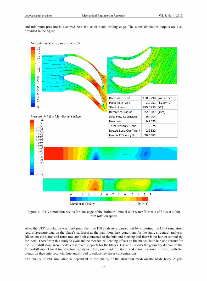
Figure 11 shows the CFD simulation results for one stage of the Turbodrill model with water flow rate of 3 L/s at the rotation speed of 4,000 rpm which is close to the optimum rotation speed. This figure shows the velocity profile in the blade to blade view at the span surface 0.5 (half way between hub and shroud). The first blade row is the stator blade row that shows increasing velocity. The second blade row is the rotor blade row that shows changing in velocity vectors, in turn, cause rotation. Some flow separations are visible on the leading and trailing edges of the blades. Also this figure shows the pressure and meridional velocity profiles at meridional surface (axi-symmetric surface between hub and shroud). The pressure and velocity profiles show the maximum velocity


16

and minimum pressure is occurred near the stator blade trailing edge. The other simulation outputs are also provided in the figure.

Figure 11. CFD simulation results for one stage of the Turbodrill model with water flow rate of 3 L/s at 4,000 rpm rotation speed

After the CFD simulation was performed then the FSI analysis is carried out by importing the CFD simulation results (pressure data on the blade’s surfaces) as the main boundary conditions for the static structural analysis. Blades on the stator and rotor row are both connected to the hub and housing and there is no hub or shroud tip for them. Therefor in this study to evaluate the mechanical loading effects on the blades, both hub and shroud for the Turbodrill stage were modelled as fixed supports for the blades. Figure 12 shows the geometry domain of the Turbodrill model used for structural analysis. Here, one blade of stator and rotor is shown in green with the blends on their interface with hub and shroud to reduce the stress concentrations.

The quality of FSI simulation is dependent to the quality of the structural mesh on the blade body. A grid


17

convergence study has been done with 4 levels of mesh refinements (from zero refinement to 3 times refinments) for the blades body of the Turbodrill stage model. Table 5 shows the mesh models information and structural analysis results for the four mesh models generated for FSI grid convergence study. This table shows that the mesh model with 2 level refinments will result at good quality simulation results with moderate mesh density on the blades body and within reasonable CPU time for the purpose of this study. As a result, this mesh model was used for the FSI analyses in this paper. Figure 13 shows the mesh model selected for FSI analysis with 2 level refinemets for the blades body.

Table 5. Simulation results for FSI grid convergence study for four mesh models

Mesh Model Total Nodes Total Elements Minimum

Maximum

Equivalent (Von-Mises) Stress

(MPa)

Equivalent Elastic Strain

(×10-4 mm/mm)

Total Deformation(×10-3 mm)

0 96,631 62,371 Min 8.597 0.471 0 Max 181.144 9.440 2.711

1 322,474 221,602 Min 9.068 0.471 0 Max 191.100 9.903 2.732

2 683,000 477,477 Min 9.048 0.472 0 Max 193.784 10.320 2.737

3 1,646,698 1,177,216 Min 9.030 0.469 0 Max 194.319 10.960 2.739

Figure 12. Geometry domain of the Turbodrill model used for structural analysis, with one blade of stator and rotor in green with the blends on their interfaces with hub and shroud

Table 6 shows structural (FSI) simulation results for water flow rate of 3 L/s at 4,000 rpm rotation speed through the Turbodrill stage model. This table shows the minimum and maximum stress, strain and deformation caused by water flow on the blades with different blend radius. The blends on the intersection of blades with hub and shroud surfaces with different blend radius were located to reduce the stress concentration on the sharp interfaces. The blade’s material was set to the software default stainless steel with Young's Modulus = 193 GPa, Shear Modulus = 73.7 GPa, Bulk Modulus = 169 GPa, Poisson’s Ratio = 0.31, and Yield Strength = 207 MPa.


18

Figure 14 shows the equivalent (Von-Mises) stress and the total deformation profile for water flow rate of 3 L/s at 4,000 rpm rotation speed through the Turbodrill stage model with blend radius of 0.5 mm. This figure shows that maximum equivalent stress of 193.599 MPa is occurred on the trailing edge of the stator blade at its interface with shroud, and the maximum total deformation of 2.732×10-3 mm is occurred on the trailing edge of the stator blade at the middle distance between hub and shroud.

Figure 13. Mesh model selected for FSI analysis with 2 level refinemets for the blades body

Figure 14. Structural (FSI) simulation results for water flow rate of 3 L/s at 4,000 rpm rotation speed through the Turbodrill stage model with blend radius of 0.5 mm


19

Table 6. FSI simulation results for water flow rate of 3 L/s at 4,000 rpm rotation speed

Static Structural Analysis Equivalent

(Von-Mises) Stress(MPa)


(×10-4 mm/mm)


Blend Radius = 0.0 mm Min 8.847 0.479 0 Max 302.649 24.655 2.812



Figures 15 and 16 show the CFD simulation results for one stage of the Turbodrill model with water flow rate of 4 L/s. The maximum stage efficiency and power for this case is at around 6,000 revolutions per minute (rpm) rotation speed. One stage power and torque at maximum efficiency condition are around 725 W and 1152 N.mm, respectively. In this case, the runaway turbine speed is almost over 11,000 rpm, and stalled torque is around 2320 N.mm. Figure 16 shows the CFD simulation results the rotation speed of 6,000 rpm which is close to the optimum rotation speed. This figure shows the velocity profile in the blade to blade view at the span surface 0.5 (half way between hub and shroud). Some flow separations are visible on the leading and trailing edges of the blades. Also this figure shows the pressure and meridional velocity profiles at meridional surface (axi-symmetric surface between hub and shroud). The pressure and velocity profiles show the maximum velocity and minimum pressure is occurred near the stator blade trailing edge. The other simulation outputs are also provided in the figure.

R² = 0.9978

R² = 0.9992

0

600

1200

1800

2400

0

200

400

600

800

0 2000 4000 6000 8000 10000 12000

One

Sta

ge T

orqu

e (N

.mm

)

One

Sta

ge P

ower

(W

)


Power

Torque

Figure 15. CFD simulation results for one stage of the Turbodrill model with water flow rate of 4 L/s at its reference radius of 22.5987 mm

Table 7 shows structural (FSI) simulation results for water flow rate of 4 L/s at 6,000 rpm rotation speed through the Turbodrill stage model. This table shows the minimum and maximum stress, strain and deformation caused by water flow on the blades with two different blend radiuses.


20

Table 7. FSI simulation results for water flow rate of 4 L/s at 6,000 rpm rotation speed

Static Structural Analysis Equivalent

(Von-Mises) Stress(MPa)


(×10-4 mm/mm)




Figure 16. CFD simulation results for one stage of the Turbodrill model with water flow rate of 4 L/s at 6,000 rpm rotation speed

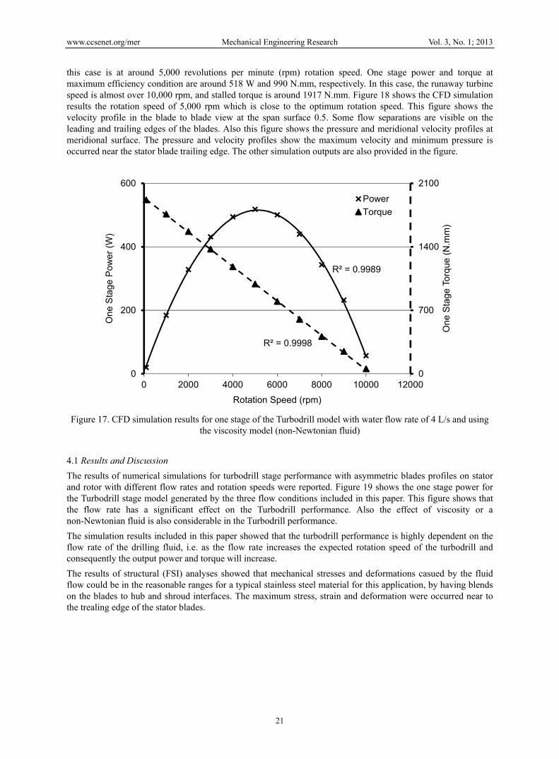
Figures 17 and 18 show water flow CFD simulation results for one stage of the Turbodrill model with water flow rate of 4 L/s and using the viscosity model (non-Newtonian fluid). The maximum stage efficiency and power for


21

this case is at around 5,000 revolutions per minute (rpm) rotation speed. One stage power and torque at maximum efficiency condition are around 518 W and 990 N.mm, respectively. In this case, the runaway turbine speed is almost over 10,000 rpm, and stalled torque is around 1917 N.mm. Figure 18 shows the CFD simulation results the rotation speed of 5,000 rpm which is close to the optimum rotation speed. This figure shows the velocity profile in the blade to blade view at the span surface 0.5. Some flow separations are visible on the leading and trailing edges of the blades. Also this figure shows the pressure and meridional velocity profiles at meridional surface. The pressure and velocity profiles show the maximum velocity and minimum pressure is occurred near the stator blade trailing edge. The other simulation outputs are also provided in the figure.

R² = 0.9989

R² = 0.9998

0

700

1400

2100

0

200

400

600

0 2000 4000 6000 8000 10000 12000

One

Sta

ge T

orqu

e (N

.mm

)

One

Sta

ge P

ower

(W

)


Power

Torque

Figure 17. CFD simulation results for one stage of the Turbodrill model with water flow rate of 4 L/s and using the viscosity model (non-Newtonian fluid)

4.1 Results and Discussion

The results of numerical simulations for turbodrill stage performance with asymmetric blades profiles on stator and rotor with different flow rates and rotation speeds were reported. Figure 19 shows the one stage power for the Turbodrill stage model generated by the three flow conditions included in this paper. This figure shows that the flow rate has a significant effect on the Turbodrill performance. Also the effect of viscosity or a non-Newtonian fluid is also considerable in the Turbodrill performance.

The simulation results included in this paper showed that the turbodrill performance is highly dependent on the flow rate of the drilling fluid, i.e. as the flow rate increases the expected rotation speed of the turbodrill and consequently the output power and torque will increase.

The results of structural (FSI) analyses showed that mechanical stresses and deformations casued by the fluid flow could be in the reasonable ranges for a typical stainless steel material for this application, by having blends on the blades to hub and shroud interfaces. The maximum stress, strain and deformation were occurred near to the trealing edge of the stator blades.


22

Figure 18. CFD simulation results for one stage of the Turbodrill model with water flow rate of 4 L/s at 5,000 rpm rotation speed and using the viscosity model (non-Newtonian fluid)


23

0

200

400

600

800

0 2000 4000 6000 8000 10000 12000

On

e S

tag

e P

ow

er

(W)


4 L/s flow rate, Visocisity Model

4 L/s flow rate

3 L/s flow rate

Figure 19. One stage power for the Turbodrill stage model generated by the three different flow conditions

5. Conclusion

Basic design methodology for multistage Turbodrill (turbine down hole motor) optimized for small size Coiled Tube (CT) Turbodrilling system for deep hard rocks mineral exploration applications was presented. In the design methodology presented in this paper, Computational Fluid Dynamics (CFD) code was used at the first stage to analyze the fluid flow performance through Turbodrill and then Fluid-Structural Interaction (FSI) analyses were used to calculate the amount of the mechanical stresses and deformations caused by the fluid flow and interactions with the blades.

This paper reported a few simulation results for small diameter Turbodrill design optimization for minimum drilling fluid flow rate, while generating required power and speed. The software platform capable of predicting Turbodrill performance and flow properties passing motor, for any complex drilling fluid (multiphase flow, multi-components fluid) in any possible conditions was proposed which makes the Turbodrilling optimization more straightforward in comparison with the previous platforms that are passive and only check the Turbodrill performance through limited lab experiment flow test, with restricted fluid flow observations.

Acknowledgements

The authors would like to express their sincere thanks to the Deep Exploration Technologies Cooperative Research Centre (DET CRC) for their financial supports towards this project. This paper is the DET CRC document 2012/086.

References

ANSYS. (2011). ANSYS Software Reference Booklets. Release 14.0, Copyright © 2011, Retrieved from http://www.ansys.com

Beaton, T., & Seale, R. (2004). The Use of Turbodrills in Coiled Tubing Applications. Paper Presented at the SPE/ICoTA Coiled Tubing Conference (SPE 89434), Houston, Texas, USA.

Dixon, S. L., & Hall, C. A. (2010). Fluid Mechanics and Thermodynamics of Turbomachinery. United States of America: Elsevier Inc.

Eskin, M., & Maurer, W. C. (1997). Advanced Downhole Drilling Motors. Maurer Engineering Inc.

IT. (2007). Advanced Ultra-High Speed Motor for Drilling. (Impact Technologies LLC). Tulsa, Oklahoma, Final Report, US Department of Energy, National Energy Technology Laboratory (NETL).


24

Lyons, W. C., & Plisga, G. J. (2005). Standard Handbook of Petroleum & Natural Gas Engineering, United States of America, Elsevier Inc.

Menter, F. R. (1994). Two-equation eddy-viscosity turbulence models for engineering applications. AIAA-Journal, 32(8), 269-289.

Mokaramian, A., Rasouli, V., & Cavanough, G. (2012). Adapting oil and gas downhole motors for deep mineral exploration drilling. In Deep Mining 2012: Proceedings of the sixth International Seminar on Deep and High Stress Mining, pp. 475-486, Australian Centre for Geomechanics (ACG), Perth, Western Australia.

Mokaramian, A., Rasouli, V., & Cavanough, G. (2012). A feasibility study on adopting coiled tubing drilling technology for deep hard rock mining exploration. In Deep Mining 2012: Proceedings of the sixth International Seminar on Deep and High Stress Mining, pp. 487-499, Australian Centre for Geomechanics (ACG), Perth, Western Australia.

Natanael, M., Nevlud, K. M., Beaton, T., & Beylotte, J. (2008). Turbodrill with asymetric stator and rotor vanes. US Patent, USA: Smith International, Inc.

Radtke, R., Glowka, D., Rai, M. M., Beaton, T., & Seale, R. (2011). High-Power Turbodrill and Drill Bit for Drilling With Coiled Tubing. Technology International, Inc., US Department of Energy, National Energy Technology Laboratory (NETL).

Reich, M., Picksak, A., John, W., & Regener, T. (2000). Competitive Performance Drilling with High-Speed Downhole Motors in Hard and Abrasive Formations. Paper Presented at the IADC/SPE Drilling Conference (IADC/SPE 59215), New Orleans, Louisiana.

RIO. (2004). Current Capabilities of Hydraulic Motors, Air/Nitrogen Motors, and Electric Downhole Motors. (RIO Technical Services). Final Report, US Department of Energy.

Sanchez, A., Samuel, G. R., & Johnson, P. (1996). An Approach for the Selection and Design of Slim Downhole Motors for Coiled Tubing Drilling. Paper Presented at the SPE Horizontal Drilling Conference (SPE 37054), Calgary, Canada.

fluid flow investigation through small turbodrill for

Documents