Optically Inaccessible Flow

Visualization using Positron

Emission TomographyNMSU PHYSICS DEPT. COLLOQUIUM PRESENTATION

JEREMY BRUGGEMANN

MAY 4TH, 2018

1

Outline Introduction

Motivation for Positron Emission Tomography

Background

PET Physics & Instrumentation

Concept Description

Advantages

Literature Survey - Optically Inaccessible Flow Visualization

Experimental Research

Objectives

Test Methodology

Results & Discussion

Conclusions

Current Work – Static Fluid Distribution & Steady State Flow Visualization

Future Work - Steady State and Periodically Transient Flow Field visualization

2

Introduction Flow visualization is powerful tool in

characterizing fluid dynamics in engineering systems

Anchor models used for developing system designs

Performance characterization using quantitative flow field velocimetry and scalar transport mapping

Most current techniques require optical accessibility of the flow or probes

View ports and probes on integrated systems may not be feasible

Compromise structural integrity

Intrusive to the flow field

Lab scale testing may need to be performed with view ports

As built configurations and conditions may deviate from lab scale test conditions

Unable to conduct performance anomaly diagnostics, e.g. identify obstructed flow

3

Laser Induced

Fluorescence –

scalar imaging

technique

(Source: Ref.

1)

Laboratory-scale

optically accessible

combustor

equipped with a

single-element shear

coaxial injector

(Source: Ref. 2)

Performance

impact due to flow

obstruction

Motivation Flow visualization of optically inaccessible

flows is needed to characterize flow within as-built, integrated systems

A Possible Solution: Positron Emission Tomography (PET)

Used widely in the medical field to non-intrusively visualize 3D fluid distributions in humans and small animals

Used to diagnose physiological processes

PET Technology is becoming more relevant to applications in engineering field

Silicon Photo Multipliers (SiPMs)/ Avalanche Photo Diodes (APD) replaces traditional PMTs – increased signal to noise ratio

Lutetium Yttrium Oxyorthosilicate (LYSO) scintillation material replacing NaIscintillators

Shorter scintillation decay time – reduced dead time

Increased gamma-ray stopping power

Enables Time-of-Flight (TOF) reconstruction algorithm

4

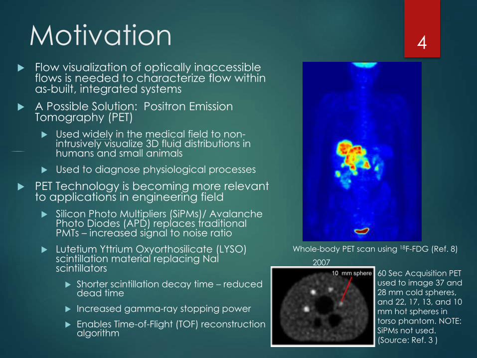
60 Sec Acquisition PET

used to image 37 and

28 mm cold spheres,

and 22, 17, 13, and 10

mm hot spheres in

torso phantom. NOTE:

SiPMs not used.

(Source: Ref. 3 )

Whole-body PET scan using 18F-FDG (Ref. 8)

2007

BackgroundPET PHYSICS & INSTRUMENTATIONCONCEPT DESCRIPTIONADVANTAGESLITERATURE SURVEY

5

PET Physics & Instrumentation Beta+ Decay

Unstable radioisotopes emit positrons with initial kinetic energy

Kinetic energy reduced through interaction with surrounding media until sufficiently low to annihilate with electrons

Produces two nearly collinear 511 keVgamma-rays propagating in opposite directions

PET Detectors

Gamma-rays interact (primarily Compton scatter) with scintillating crystals emitting optical photons

Optical photons are detected by PMTs/SiPMs

Single detections are processed to identify coincident detections within specified time window

Coincident detections = Line of Response (LOR) between triggered detectors

Multiple LORs and time-of-flight (TOF) data used to reconstruct radioisotope distribution

6

Measured LORs

for 3 ml slug of F-

18/water solution

in Modular Unit

at Positron

Imaging Centre

of Univ. of

Birmingham, UK

Conceptual schematic of PET applied to visualizing

flow in a pipe (Modified from Ref. 8)

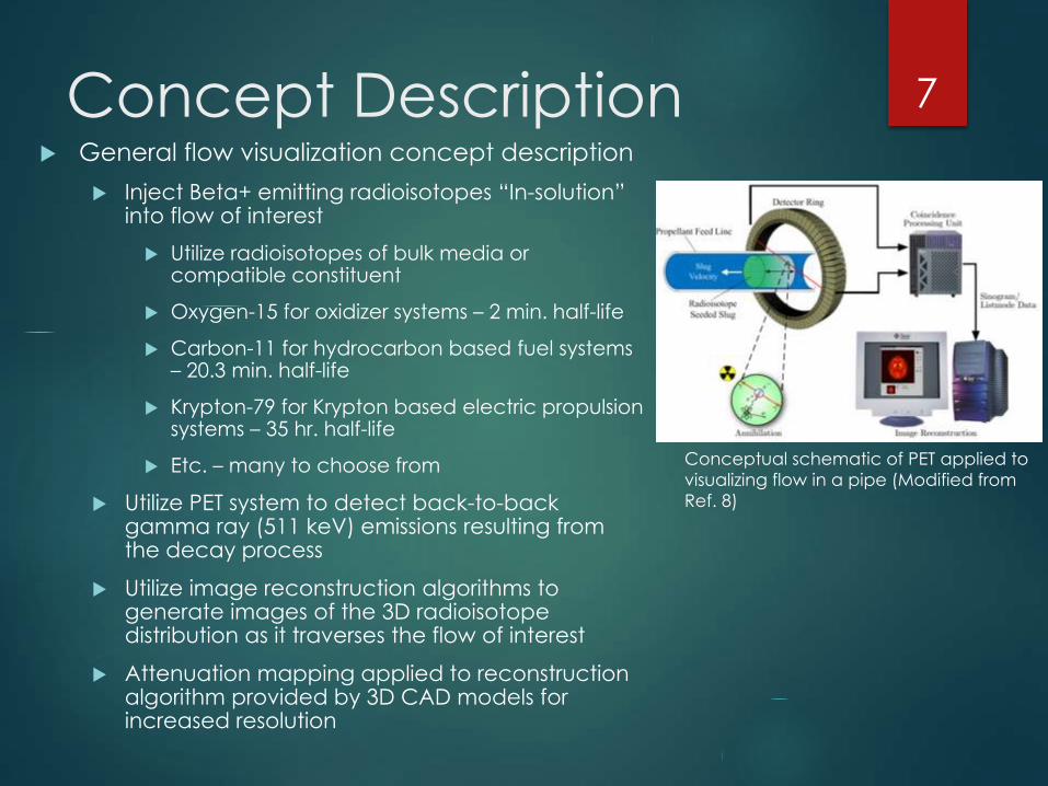
Concept Description General flow visualization concept description

Inject Beta+ emitting radioisotopes “In-solution” into flow of interest

Utilize radioisotopes of bulk media or compatible constituent

Oxygen-15 for oxidizer systems – 2 min. half-life

Carbon-11 for hydrocarbon based fuel systems – 20.3 min. half-life

Krypton-79 for Krypton based electric propulsion systems – 35 hr. half-life

Etc. – many to choose from

Utilize PET system to detect back-to-back gamma ray (511 keV) emissions resulting from the decay process

Utilize image reconstruction algorithms to generate images of the 3D radioisotope distribution as it traverses the flow of interest

Attenuation mapping applied to reconstruction algorithm provided by 3D CAD models for increased resolution

7

Conceptual schematic of PET applied to

visualizing flow in a pipe (Modified from

Ref. 8)

Advantages Benefits of flow/fluid distribution visualization of

optically inaccessible flow fields with PET Technology

Gamma rays are highly energetic (511 keV) enabling

penetration of fluid containment materials

Fluid dynamics of fully integrated systems can be

characterized

Using radioisotope of the bulk media preserves

thermochemical properties during visualization process

radiobiological hazards mitigated due to relatively

short radioisotope half lives, e.g. 2 minutes for O-15

3D CAD models of engineering system can be

superimposed on 3D radioisotope distribution data for

high fidelity visualization

8

1988 - Bearing rig oil

injection visualization – 3D

CAD model superimposed

(Source: Ref.4)

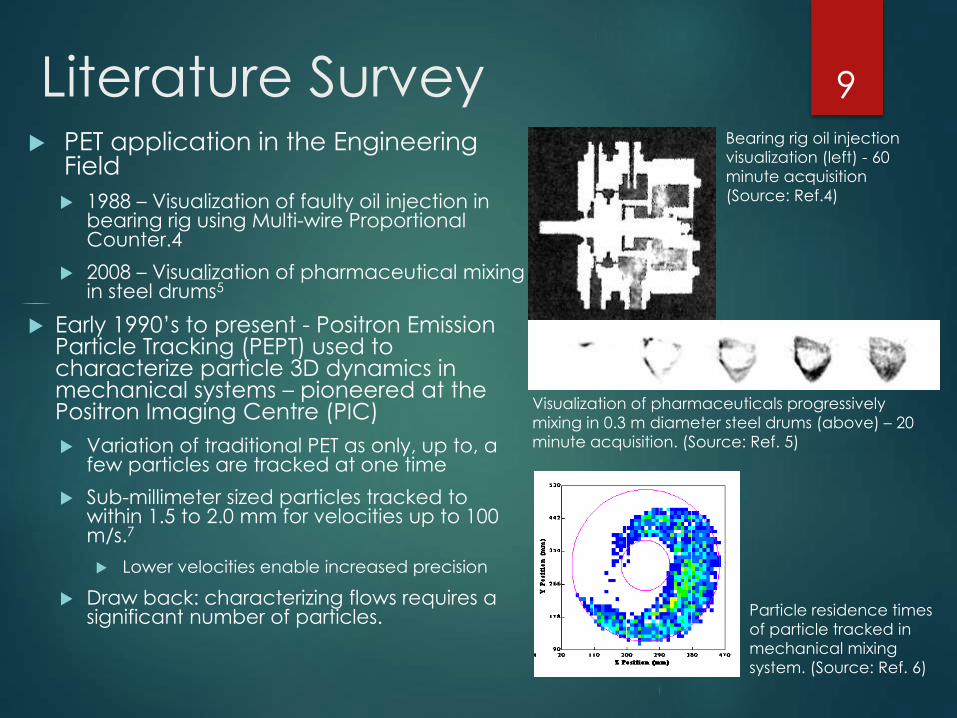
Literature Survey PET application in the Engineering

Field

1988 – Visualization of faulty oil injection in bearing rig using Multi-wire Proportional Counter.4

2008 – Visualization of pharmaceutical mixing in steel drums5

Early 1990’s to present - Positron Emission Particle Tracking (PEPT) used to characterize particle 3D dynamics in mechanical systems – pioneered at the Positron Imaging Centre (PIC)

Variation of traditional PET as only, up to, a few particles are tracked at one time

Sub-millimeter sized particles tracked to within 1.5 to 2.0 mm for velocities up to 100 m/s.7

Lower velocities enable increased precision

Draw back: characterizing flows requires a significant number of particles.

9

Visualization of pharmaceuticals progressively

mixing in 0.3 m diameter steel drums (above) – 20

minute acquisition. (Source: Ref. 5)

Particle residence times

of particle tracked in

mechanical mixing

system. (Source: Ref. 6)

Bearing rig oil injection

visualization (left) - 60

minute acquisition

(Source: Ref.4)

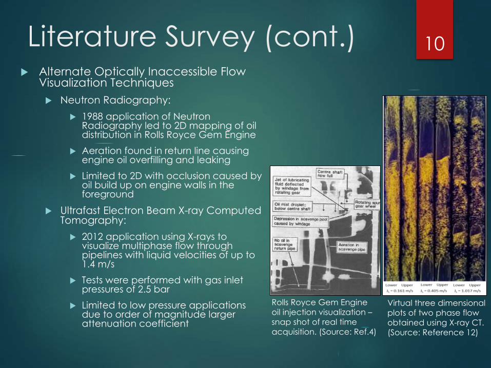
Literature Survey (cont.) Alternate Optically Inaccessible Flow

Visualization Techniques

Neutron Radiography:

1988 application of Neutron Radiography led to 2D mapping of oil distribution in Rolls Royce Gem Engine

Aeration found in return line causing engine oil overfilling and leaking

Limited to 2D with occlusion caused by oil build up on engine walls in the foreground

Ultrafast Electron Beam X-ray ComputedTomography:

2012 application using X-rays to visualize multiphase flow through pipelines with liquid velocities of up to1.4 m/s

Tests were performed with gas inlet pressures of 2.5 bar

Limited to low pressure applications due to order of magnitude larger attenuation coefficient

10

Virtual three dimensional

plots of two phase flow

obtained using X-ray CT.

(Source: Reference 12)

Rolls Royce Gem Engine

oil injection visualization –

snap shot of real time

acquisition. (Source: Ref.4)

Experimental ResearchPOSITRON IMAGING CENTRE – UNIVERSITY OF

BIRMINGHAM, UNITED KINGDOM

11

Objectives Overall objective: Parametrically bound the applicable

flow fields that can be sufficiently visualized using

current PET systems

Requires characterization of PET systems’ dynamic resolution

(i.e. achievable spatial resolution using data acquired within a

specified unit of time) and count rate performance

Experiment Objective

Measure the dynamic resolution for the ADAC Forte Gamma

Camera and Modular PET Unit located at the Positron Imaging

Centre

Measure the peak count rates for the ADAC Forte Gamma

Camera and Modular PET Unit

Use measurements to begin establishing a correlation that can

be extrapolated to approximate a PET system’s dynamic

resolution given it’s measured Peak NECR

12

Dynamic Resolution

Measurements

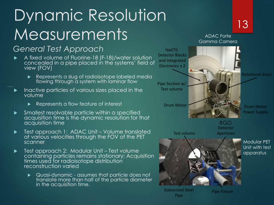
A fixed volume of Fluorine-18 (F-18)/water solution concealed in a pipe placed in the systems’ field of view (FOV)

Represents a slug of radioisotope labeled media flowing through a system with laminar flow

Inactive particles of various sizes placed in the volume

Represents a flow feature of interest

Smallest resolvable particle within a specified acquisition time is the dynamic resolution for that acquisition time

Test approach 1: ADAC Unit – Volume translated at various velocities through the FOV of the PET scanner

Test approach 2: Modular Unit – Test volume containing particles remains stationary; Acquisition times used for radioisotope distribution reconstruction varied

Quasi-dynamic - assumes that particle does not translate more than half of the particle diameter in the acquisition time.

13

General Test Approach

ADAC Forte

Gamma Camera

NaI(Tl)

Modular PET

Unit with test

apparatus

BGO

Test Apparatus Fluid containment

10 mL syringe with plunger located at the 3 mL indicator

Non-Activated Particles

Diameters: 3.0 ± 0.1 mm, 5.0 ± 0.1 mm, 8.0 ± 0.1 mm

Adhered to tip of interchangeable syringe plungers

Syringe with test volume friction fit in steel pipe up to stopping flange

ADAC - Pipe connected to rotational drum at 140 mm radius (series 1) and 70 mm (series 2 - shown in figure)

Modular – syringe at single location

14

Fluid containment

with cross sectional

geometry of test volume

(inset)

ADAC Unit Test Setup

3, 5, and 8 mm particles adhered

to interchangeable plungers

Modular Unit Test

Apparatus

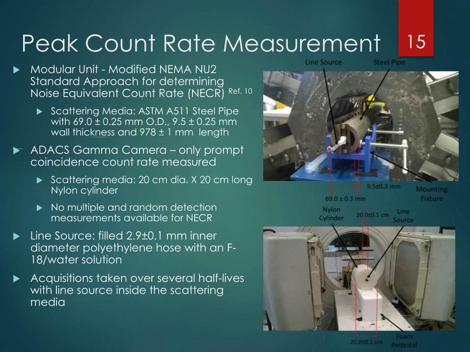
Peak Count Rate Measurement Modular Unit - Modified NEMA NU2

Standard Approach for determining Noise Equivalent Count Rate (NECR) Ref. 10

Scattering Media: ASTM A511 Steel Pipe with 69.0 ± 0.25 mm O.D., 9.5 ± 0.25 mm wall thickness and 978 ± 1 mm length

ADACS Gamma Camera – only prompt coincidence count rate measured

Scattering media: 20 cm dia. X 20 cm long Nylon cylinder

No multiple and random detection measurements available for NECR

Line Source: filled 2.9±0.1 mm inner diameter polyethylene hose with an F-18/water solution

Acquisitions taken over several half-lives with line source inside the scattering media

15

Post-Test Processing Image Reconstruction Algorithms

ADAC: Simple 2D back projection

User specified mid-volume plane, slice thickness and acquisition duration

Each projection is 1 mm thick and contains 1 mm x 1 mm pixels

Pixel value represents number of LORs that intersected the pixel on the projection plane

Modular Unit: simple, 3D back projection

Adapted from PEPT algorithm

Each voxel intersected by a detected LOR incrementally increased

Voxel size: 1 mm x 1 mm x 1mm

Disclaimer: Neither algorithm is representative of state-of-the-art nor are they representative of higher performing Filtered Back Projection (FBP) algorithms (standard algorithm used in tomography)

16

Conceptual schematic of ADAC Unit image

reconstruction algorithm (modified from Ref.

5)

Measured LORs

for 3 ml slug of F-

18/water solution

in Modular Unit

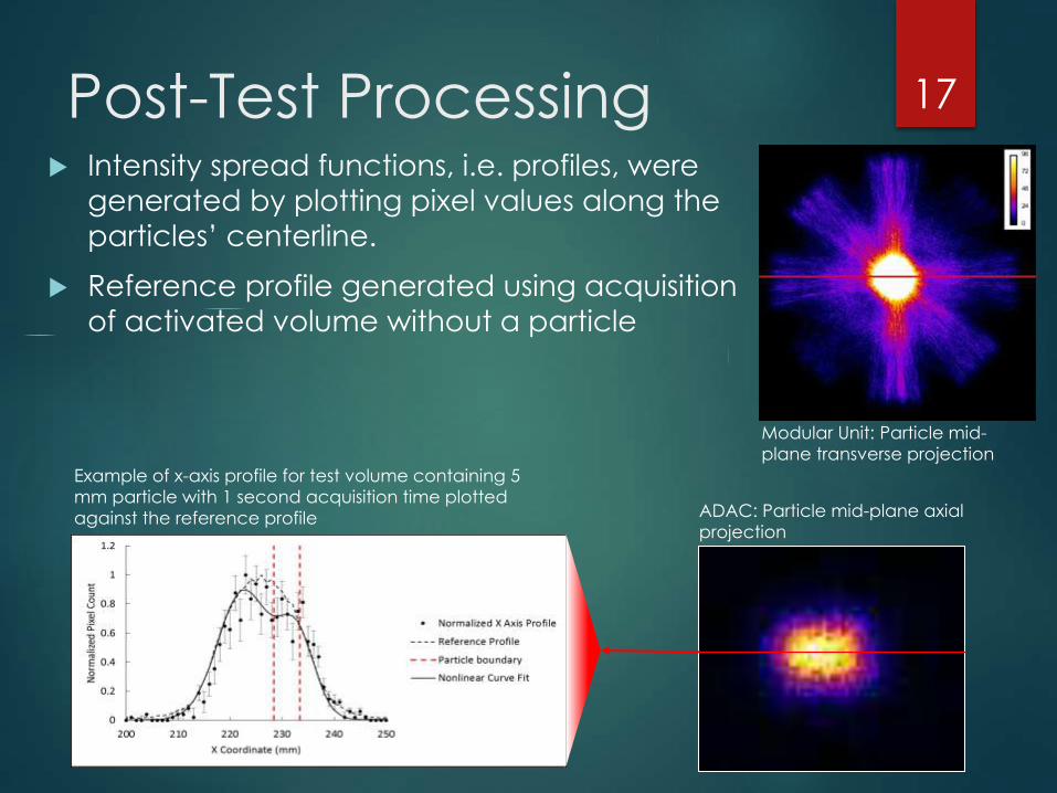
Post-Test Processing Intensity spread functions, i.e. profiles, were

generated by plotting pixel values along the

particles’ centerline.

Reference profile generated using acquisition

of activated volume without a particle

17

Example of x-axis profile for test volume containing 5

mm particle with 1 second acquisition time plotted

against the reference profile ADAC: Particle mid-plane axial

projection

Modular Unit: Particle mid-

plane transverse projection

RESULTS AND DISCUSSIONDISCLAIMER: POST PROCESSING RESULTS ARE

PRELIMINARY IN NATURE.

18

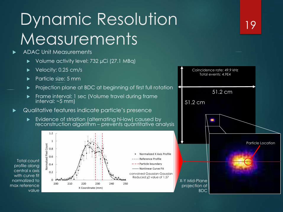
Dynamic Resolution

Measurements ADAC Unit Measurements

Volume activity level: 732 µCi (27.1 MBq)

Velocity: 0.25 cm/s

Particle size: 5 mm

Projection plane at BDC at beginning of first full rotation

Frame interval: 1 sec (Volume travel during frame interval: ~5 mm)

Qualitative features indicate particle’s presence

Evidence of striation (alternating hi-low) caused by reconstruction algorithm – prevents quantitative analysis

19

51.2 cm

51.2 cm

X-Y Mid-Plane

projection at

BDC

Coincidence rate: 49.9 kHz

Total events: 4.9E4

Particle Location

Total count

profile along

central x axis

with curve fit

normalized to

max reference

value

convolved Gaussian-Gaussian

Reduced χ2 value of 1.57

Dynamic Resolution

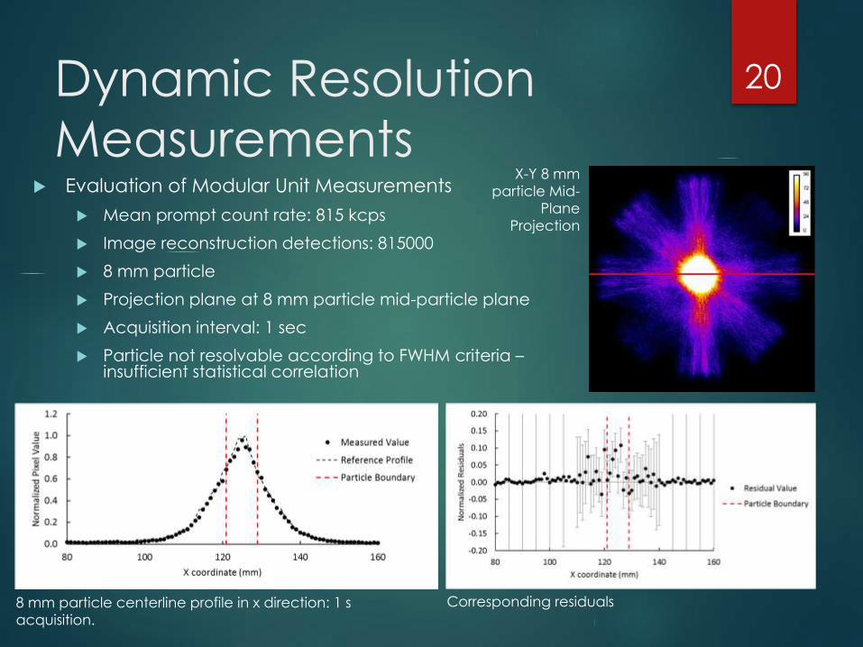
Measurements Evaluation of Modular Unit Measurements

Mean prompt count rate: 815 kcps

Image reconstruction detections: 815000

8 mm particle

Projection plane at 8 mm particle mid-particle plane

Acquisition interval: 1 sec

Particle not resolvable according to FWHM criteria –insufficient statistical correlation

20

X-Y 8 mm

particle Mid-

Plane

Projection

8 mm particle centerline profile in x direction: 1 s

acquisition.

Corresponding residuals

Dynamic Resolution Measurements Increased acquisition window for increased

detections

Mean prompt count rate: 815 kcps

Image reconstruction detections: 8,150,000

8 mm particle

Projection plane at 8 mm particle mid-particle plane

Acquisition interval: 10 sec

Effective velocity: 0.04 cm/s

Velocity = particle radius / acquisition time

FWHM: 6.84 ± 0.31 mm

Lower than particle diameter - Suggests inaccurate quantitative results - particle qualitatively resolved

21

X-Y 8 mm

particle Mid-

Plane

projection

8 mm particle centerline profile in x direction: 10 s

acquisitionCorresponding residuals

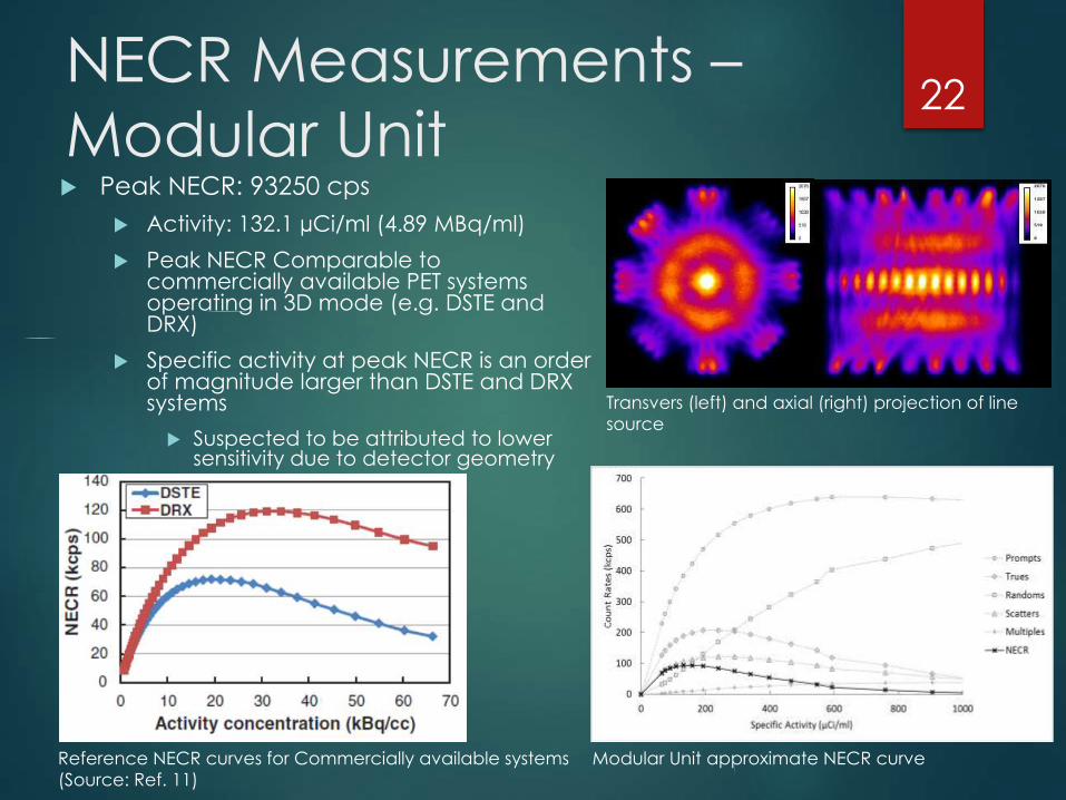
NECR Measurements –

Modular Unit Peak NECR: 93250 cps

Activity: 132.1 µCi/ml (4.89 MBq/ml)

Peak NECR Comparable to commercially available PET systems operating in 3D mode (e.g. DSTE and DRX)

Specific activity at peak NECR is an order of magnitude larger than DSTE and DRX systems

Suspected to be attributed to lower sensitivity due to detector geometry

22

Reference NECR curves for Commercially available systems

(Source: Ref. 11)

Transvers (left) and axial (right) projection of line

source

Modular Unit approximate NECR curve

Peak Count Rate

Measurement – ADAC Unit Only Prompt Coincident

Count Rate measured

Randoms and multiples

measurements not

available

Peak Prompt Count Rate:

~63,000 cps

Peak NECR must be below

this count rate.

23

ADAC Unit optimal specific activity curve

Axial projection of

line source used for

ADAC count rate

measurement

Dynamic Resolution – Peak

Count Rate Correlation Research to this point has only

produced two rudimentary data points – Shown in table.

Lower dynamic resolution of modular unit despite higher peak count rate

Attributed to lower performing modular unit reconstruction algorithm

Key note: Peak NECR alone is not sufficient metric for cross PET system comparison

Reconstruction algorithm needs to be considered and standardized across all system comparisons

Investigating use of sinogram-based FBP reconstruction algorithm

Difficult to implement for the ADAC since it is a “gamma camera” with non-axisymmetric detector configuration

24

System ADAC* Modular

Peak Count Rate (kcps) 63 93.3

Resolvable Particle (mm) 5 8

Acquisition Time (sec) 1 10

Velocity (cm/s) 0.25 0.04

Specific Activity

(kBq/mL) 15000 4890

μCi/mL 405.4 132.2

Table. Tabulated results of dynamic resolution

and peak count rate measurements.

* ADAC unit peak count rate is based on

prompt coincident count rates and is only

intended to reflect a maximum possible count

rate.

Conclusions Testing was performed to measure the

dynamic resolution and peak count rate of the ADAC Forte Positron Camera and the Modular Unit located at the Positron Imaging Centre.

Limitations from both reconstruction algorithms prevented quantitative resolution of the particles

Qualitative indications in the particle center line profiles were used to facilitate cross system comparison between ADAC and modular units

Preliminary results indicate that, despite the modular units superior count rate performance, the higher performing ADAC image reconstruction algorithm enabled the ADAC unit to have a higher dynamic resolution.

No dynamic resolution – peak count rate correlation established for cross system comparison

Standardized image reconstruction algorithm needs to be implemented

25

Current WorkSTEADY STATE FLUID FLOW & STATIONARY FLUID

DISTRIBUTION VISUALIZATION

26

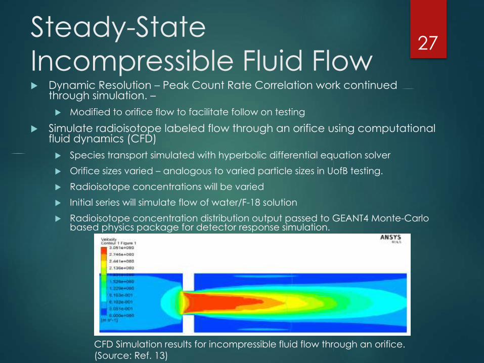
Steady-State

Incompressible Fluid Flow Dynamic Resolution – Peak Count Rate Correlation work continued

through simulation. –

Modified to orifice flow to facilitate follow on testing

Simulate radioisotope labeled flow through an orifice using computational fluid dynamics (CFD)

Species transport simulated with hyperbolic differential equation solver

Orifice sizes varied – analogous to varied particle sizes in UofB testing.

Radioisotope concentrations will be varied

Initial series will simulate flow of water/F-18 solution

Radioisotope concentration distribution output passed to GEANT4 Monte-Carlo based physics package for detector response simulation.

27

CFD Simulation results for incompressible fluid flow through an orifice.

(Source: Ref. 13)

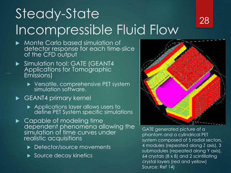
Steady-State

Incompressible Fluid Flow Monte Carlo based simulation of

detector response for each time-slice of the CFD output

Simulation tool: GATE (GEANT4 Applications for Tomographic Emissions)

Versatile, comprehensive PET system simulation software.

GEANT4 primary kernel

Applications layer allows users to define PET System specific simulations

Capable of modeling time dependent phenomena allowing the simulation of time curves under realistic acquisitions

Detector/source movements

Source decay kinetics

28

GATE generated picture of a

phantom and a cylindrical PET

system composed of 5 radial sectors,

4 modules (repeated along Z axis), 3

submodules (repeated along Y axis),

64 crystals (8 x 8) and 2 scintillating

crystal layers (red and yellow)

Source: Ref 14)

Zero-Gravity Propellant Gauging Methods for propellant gauging in gravity field

are not effective in zero-G conditions – liquid level not identifiable

Traditional methods of zero-G propellant gauging are subject to 3% uncertainty and greater as well as other drawbacks

Equation-of-state (EOS) estimations (usually the ideal gas law)

Pressure and temperature of the ullage volume in the tank is monitored – used to calculate volume based on EOS.

Requires the additional hardware of pressurant tanks, pumps, valves and other hardware necessary to transfer pressurant

Measurement of spacecraft dynamics

Propulsion system activated and spacecraft dynamics measured – used to determine over all mass of the spacecraft

Mass estimated by removing dry mass of spacecraft from overall mass estimation.

Consumes Propellant

Burn-time Integration.

Book-keeping method - Total propellant usage is estimated via assumptions about the propellant use during each thruster firing

Subject to large uncertainties from assumptions about thruster operating performance

29

Propellant Distribution in

quiescent zero-G state

Wall

Liquid

Gas

Zero-Gravity Propellant

Gauging with PET Concept Description

Concept 1:

Saturate Fuel and/or NTO bulk propellant with Kr-79 Analogous to the mercaptan additive introduced to

natural gas to give it an odor for easier detection.

Concept 2:

Inject Kr-79 into ullage volume

Utilize state of the art in PET time-of-flight (TOF) gamma ray detectors to triangulate gamma-gamma (511 keV) emission sources

Kr-79: 35 hr. half-life – 17 days of mission coverage

Propellant Gauging Algorithm

2D mapping of the liquid-gas interface through cross-sectional slice of tank at detector planes Onboard algorithm generates 3D axisymmetric projection

Onboard void fraction algorithm used to calculate volumetric measurement of propellant.

Create test-validated models of void fraction vs propellant quantity.

Integrate sensor and model results to determine correction factors for increased accuracy.

30

Planar Cross Section

Notional Detector Configuration

X

Y

Z

Assessment Plan Objective:

Evaluate the ability of the shown detector configuration and proposed algorithm to accurately (< 3% uncertainty of full scale) measure the quantity of propellant in the tank.

Approach:

Use GATE to simulate various detector configurations and source distributions

Source distributions will vary to represent multiple fill levels

Full, Half Full, Near Empty

Radioisotope concentrations, i.e. specific activity levels, will vary to represent measurement acquisitions at various points during the mission

Start of Mission (Day 1), Mid Mission (Day 8), End of Mission (Day 17)

31

X

Y

Z

Future WorkSTEADY STATE AND PERIODICALLY TRANSIENT FLOW

FIELD VISUALIZATION

32

Electric Propulsion Devices Propellant:

Xenon, Krypton, Iodine

Technical Challenge:

Results from modeling indicate that there is as much as 6% variation in maximum thrust efficiency simply due to the method of ionization.

Currently it is not apparent how or where this loss can be measured in thruster data.

Possible Solution:

Ionization Efficiency characterization using Positron emission tomography

β+ Radioisotope of bulk propellant

Kr-79: Half Life: 35 hrs

33

NASA JPL developed ion thruster during a

test firing. A quartet of these highly efficient

T6 thrusters is being installed on ESA’s

BepiColombo spacecraft to Mercury.

(source: Ref. 15)

Concept Description Positron-electron annihilation

occurs only once positron

kinetic energy is sufficiently

reduced through interactions

with surrounding atoms

Coulombic forces from

propellant ions repel positrons

Reduces resident time near

electron orbitals of ionic atoms

Reduces positron-electron

annihilation cross-section

Results in correlation between

localized detection rate and

local ionization level

34

Anticipated Radioisotope

detection mapping in an

ion thruster using Positron

Emission Tomography.

(Modified from Ref. 16)

7 mm dia. orifices

(range 3 mm to 10

mm)

Clogged orifice PlateOrifice Plate

Broader Industrial

Applications Flow feature/obstruction

Characterization

Steady-state flow continuous

radioisotope injection

Phase Averaging of pulsed

radioisotope injection

Flow field velocimetry using

pulsed radioisotope injection

Periodically transient flow feature

characterization

35

Conceptual technique for

flow field velocity mapping

using phase averaging of

pulsed radioisotope

injection

Conceptual density

gradient rocket engine

diagnostic application.

Flow obstruction

visualization proof of

concept test apparatus

References1. “Tracer Laser Induced Fluorescence.” Universität Duisburg-Essen, March 17,

2014. Web. June 12, 2015

2. Dai, Jian, et al. “Experimental investigations of coaxial injectors in a laboratory-scale rocket combustor.” Aerospace Science and Technology, Vo. 59, (Dec. 2016) Pages 41-51

3. Suleman Surti, Austin Kuhn, Matthew E. Werner, Amy E. Perkins, Jeffrey Kolthammer, and Joel S. Karp. “Performance of Philips Gemini TF PET/CT Scanner with Special Consideration for Its Time-of-Flight Imaging Capabilities.”Journal Nucl Med, (2007); 48:471–480

4. Stewart, P. A. E. “Neutron and Positron Techniques for Fluid Transfer System Analysis and Remote Temperature and Stress Measurement.” Jounal of Engineering for Gas Turbines and Power. 110.2 (1988): 279-288. Print.

5. D J Parker, TWLeadbeater, X Fan, M N Hausard, A Ingram and Z Yang. “Positron imaging techniques for process engineering: recent developments at Birmingham.” Meas. Sci. Technol. 19 (2008)

6. Nuclear Physics Research Group. “Positron Imaging Centre.” University of Birmingham – Nuclear Physics Research Group. July 6th, 2012. Web. June 14, 2015 url: http://www.np.ph.bham.ac.uk/pic/pept

7. Leadbeater T.W. and Parker D.J., “Current Trends in Positiron Emission Particle Tracking.” 7th World Congress on Industrial Process Tomography, WCIPT7, 2-5 September 2013, Krakow, Poland

8. Wikipedia contributors. "Positron emission tomography." Wikipedia, The Free Encyclopedia. Wikipedia, The Free Encyclopedia, 19 May. 2015. Web. 14 Jun. 2015.

36

References (cont.)9. Bailey, Dale L., et al. Positron Emission Tomography: Basic Sciences. London:

Springer-Verlag, 2004. Print.

10. National Electronics Manufacturers Association, NEMA NU2-2012: Performance Measurements of Positron Emission Tomography. (2012)

11. Chang T., Chang G., Clark J.W., Jr., Diab R.H., Rohren E., Mawlawi O.R., “Reliability of predicting image signal-to-noise ratio using noise equivalent count rate in PET imaging.” Med. Phys. 39 (10), October 2012

12. M Beiberle et al, “Ultrafast electron beam X-ray computed tomography for 2D and 3D two-phase flow imaging.” IEEE. (2012) Print.

13. M. M. Tukiman, et al., “CFD Simulation of Flow Through an Orifice Plate.” IOP Conf. Ser.: Materials Science & Engineering, 243 (2017) paper # 012036

14. Open Gate Collaboration contributers, website: http://www.opengatecollaboration.org/home, (2017)

15. Online graphic: https://www.esa.int/spaceinimages/Images/2016/04/T6_ion_thruster_firing(2018)

16. Wikipedia contributors. (2018, April 6). Ion thruster. In Wikipedia, The Free Encyclopedia. Retrieved 04:47, April 24, 2018, from https://en.wikipedia.org/w/index.php?title=Ion_thruster&oldid=835093507

37

Backup Slides

38

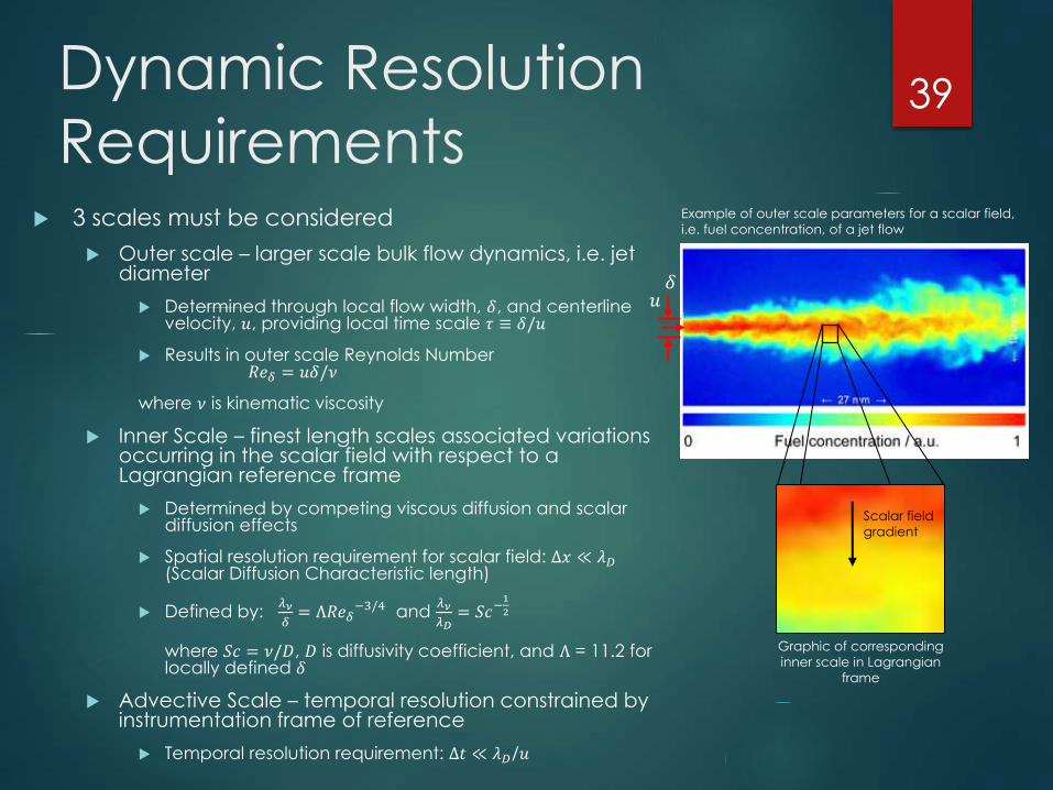
Dynamic Resolution

Requirements 3 scales must be considered

Outer scale – larger scale bulk flow dynamics, i.e. jet diameter

Determined through local flow width, 𝛿, and centerline velocity, 𝑢, providing local time scale 𝜏 ≡ 𝛿/𝑢

Results in outer scale Reynolds Number𝑅𝑒𝛿 = 𝑢𝛿/𝜈

where 𝜈 is kinematic viscosity

Inner Scale – finest length scales associated variations occurring in the scalar field with respect to a Lagrangian reference frame

Determined by competing viscous diffusion and scalar diffusion effects

Spatial resolution requirement for scalar field: ∆𝑥 ≪ 𝜆𝐷(Scalar Diffusion Characteristic length)

Defined by: 𝜆𝜈

𝛿= Λ𝑅𝑒𝛿

−3/4 and 𝜆𝜈

𝜆𝐷= 𝑆𝑐−

1

2

where 𝑆𝑐 = 𝜈/𝐷, 𝐷 is diffusivity coefficient, and Λ = 11.2 for locally defined 𝛿

Advective Scale – temporal resolution constrained by instrumentation frame of reference

Temporal resolution requirement: ∆𝑡 ≪ 𝜆𝐷/𝑢

39

𝛿𝑢

Scalar field

gradient

Example of outer scale parameters for a scalar field,

i.e. fuel concentration, of a jet flow

Graphic of corresponding

inner scale in Lagrangian

frame

Activity Concentration

Optimization Activity Concentration

Optimization

Preliminary effort required to

determine the maximum

coincidence detection rate.

Detector dead time, random,

multiple, and scattered

detections attributed to true

count rates reaching a

maximum value and then

subsiding as activity levels

increase

40

ADAC Unit optimal specific activity curve

Modular Unit optimal specific activity curve