Fluid Simulation For Computer Graphics: A Tutorial in Grid Based and ParticleBased Methods

Colin Braley∗

Virginia TechAdrian Sandu†

Virginia Tech

Figure 1: Fluid Simulation Examples

Abstract

In this paper we present a tutorial on the implementation of both agrid based and a particle based fluid simulator for computer graph-ics applications. Many research papers on fluid simulation are read-ily available, but these papers often assume a very sophisticatedmathematical background not held by many undergraduates. Fur-thermore, these papers tend to gloss over the implementation de-tails, which are very important to people trying to implement aworking system.

Recently, Robert Bridson release the wonderful book, ”Fluid Simu-lation for Computer Graphics.[Bridson 2009]” We base a large por-tion of our own grid-based simulator off of this text. However, thistext is very dense and theory intensive, and this document serves aseasy version for those who want to implement a simulator quickly.Furthermore, Bridson’s text does not cover particle based methods,like SPH, which are quickly becoming commonplace within thegraphics community. This work provides an introduction to SPHas well.

Keywords: Fluids, Physically Based Animation, SPH, Grid Based

1 Introduction

2 Introduction

In the context of physics, the word fluid may mean something dif-ferent than you might usually think. In physics, fluids fall into twocategories incompressible and compressible flow. Incompressibleflow is a liquid, such as water or juice. Compressible flow, on theother hand, corresponds to gas such as air or steam. Compressibleflow is called compressible, because you can easily change the vol-ume of this fluid. Note that there is no such thing as 100 percentincompressible fluid. All fluids, even water can change volume tosome degree. If they could not, there would be no way to audi-bly yell under water. However, we simply choose to ignore com-pressibility in fluids like water that are nearly incompressible, andinstead we refer to them simply as incompressible.

There are many, many ways to simulate fluids. In graphics, themost common two techniques are grid based simulations, and par-ticle based simulations. (Very recently, new techniques such as theLattice-Boltzmann method have been introduced to graphics, butthey are beyond the scope of this paper.) Grid based simulations

∗e-mail: cbraley@vt.edu†e-mail:sandu@cs.vt.edu

are typically highly accurate, although relatively slow comparedto particle based solutions. Particle based simulations are usuallymuch faster, but they typically do not look as good as grid basedsimulations.

Some readers may not know the difference between grid based andparticle based simulations. The best description of this can be foundin page 6 of [Bridson 2009]. I will attempt to paraphrase this de-scription here.

Fluid can be simulated from 2 viewpoints, Lagrangian or Eulerian.In the Lagrangian viewpoint, we simulate the fluid as discrete blobsof fluid. Each particle has various properties, such as mass, veloc-ity, etc. The benefit of this approach is that conservation of masscomes easily. The Eulerian viewpoint, on the other hand tracksfixed points inside of the fluid. At each fixed point, we store quan-tities such as the velocity of the fluid as it flows by, or the density ofthe fluid as it passes by. The Eulerian approach corresponds to gridbased techniques. Grid based techniques have the advantage of hav-ing higher numerical accuracy, since it is easier to work with spatialderivatives on a fixed grid, as opposed to an unstructured cloud ofparticles. However, grid based techniques often suffer from massloss, and are often slower than particle based simulations. Finally,grid based simulations often do much better tracking smooth watersurfaces, whereas particle based approaches often have issues withthese smooth surfaces.

3 Governing Equations

Here we will describe the governing equations for fluid motion, andalso describe some of the special notation used in fluid simulationliterature. For someone only interested in a basic implementation,this section can be skimmed with the exception of the final para-graph on notation. However, for a full understanding of the why influid simulation, this section should be read in full.

First, we will describe the general incompressible Navier Stokesequations. We will attempt to intuitively describe the vector cal-culus operators involved, and those without a knowledge of vectorcalculus may wish to consult the appendix of [Bridson 2009] forreview. Here are the incompressible Navier Stokes equations:

∂~u

∂t+ ~u+

1

ρ∇p = ~F + ν∇ · ∇~u (1)

∇ · ~u = 0 (2)

In these equations, ~u is fluid velocity. The time variable is t Thedensity of the fluid is represented by ρ. For water, ρ ≈ 1000 kg

m3 .The pressure inside the fluid (in force units per unit area) is repre-sented by p. Note that p and ρ are different things(the first is theGreek letter rho while the second is p). Body forces (usually justgravity) are represented by ~F . Finally, ν is the fluid’s coefficient ofkinematic viscosity.

In our simulator, we currently don’t take fluid viscosity into ac-count. For inviscid fluids like water, viscosity does usually not playa large role in the look of an animation. However, if you wish toinclude viscosity, see chapter 8 of [Bridson 2009]. The fundamen-tal work on viscous fluids in graphics is [Goktekin et al. 2004], andcan be taken as a starting point for implementation.

When the viscosity term is dropped from the incompressible NavierStokes equations, we get the following set of equations:

∂~u

∂t+

1

ρ∇p = ~F (3)

∇ · ~u = 0 (4)

These equations are simpler, and they are the equations we will con-sider for the rest of this paper. These are called the Euler Equations.

Lastly, we will quickly discuss some unique notation used in fluidsimulation. In simulation, we take small discrete time steps in or-der simulate some phenomenon. Consider the velocity field ~u be-ing simulated. In a grid based simulation, we store ~u as a discreetlysampled vector field. However, we need some type of notation todescribe which grid element we are referring to. To do this, we usesubscripts like the following ~ua,b,c to refer to the vector at a, b, c(Note that our indexing scheme is actually more complicated, butthis is discussed in the beginning of the grid based simulation sec-tion.) However, we also need a way to indicate which timestep weare referring to. To do this, we use superscripts, such as ~uk

a,b,c.The previous equation would indicate the velocity at index a, b, cat timestep k. While some would consider this an egregious abuseof notation, this syntax is extremely convenient in fluid simulation.In order to maintain clarity, we will explicitly state when we areraising a quantity to a power (as opposed to indicating a timestep).Furthermore, timesteps are written in bold (ab), whereas exponentsare written in a regular script (ab).

4 Grid Based Simulation

4.1 Overview

Here we will present a high level version of the algorithm for gridbased fluid simulation, assuming one wants to simulate n frames ofanimation.

1. Initialize Grid with some Fluid

2. for( i from 1 to n )

Let t = 0.0

While t < tframe

Calculate ∆t

Advect Fluid

Pressure Projection (Pressure Solve)

Advect Free Surface

t = t+ ∆t

Write frame i to disk

Figure 2: Our 2D Eulerian Solver

4.2 Data Structures

While we have discussed Lagrangian vs. Eulerian viewpoints, wehave yet to define what exactly we mean by ”grid” in grid basedsimulation. Throughout the simulation, we must store many dif-ferent quantities (velocity, pressure, fluid concentration, etc.) atvarious points in space. Clearly, we will lay them out in some formof regular grid. However, not just any grid will do. It turns out thatsome grids work much better than others.

Most peoples intuition is to go with the simplest approach: store ev-ery quantity on the same grid. However, for reasons which we willsoon discuss, this is not a good approach. Back in the 1950’s theseminal paper [Harlow and Welch 1965a] by Harlow and Welch de-veloped the innovate MAC Grid technique. (Note that MAC standsfor Marker-and-Cell.) Among many things, this paper developed anew way to track liquid movement through the grid, called markerparticles, and a new type of grid, a staggered grid. Marker particlesare still used in some simulators for their simplicity, but they are nolonger state of the art. However, the staggered grid developed byHarlow and Welch is still used in many, many simulators.

This grid is called staggered because it stores different quantities atdifferent locations. In two dimensions, a single cell in a MAC Gridmight look as follows:

Figure 3: Two Dimensional MAC Cell

In three dimensions, a MAC cell would look like this:

Note that in these images p represents pressure, and ~u is velocity.We see in these images that pressure is stored in the center of everygrid cell, while velocity is stored on the faces of the cells. Note thatthese velocity samples are the normal component of the velocity at

Figure 4: Three Dimensional MAC Cell

each cell face. We will now describe why the grid is arranged inthis manner.

Consider a quantity w sampled at discrete locationsw0, w1, . . . wi−1, wi, wi+1, . . . wn−1, wn along the real line.Imagine we want to estimate the derivative at some sample point i.We must use central differences of some form. Immediately, onecan see that:

∂w

∂x i≈ wi+1 − wi−1

2∆x(5)

Recall from numerical analysis that this isO(∆x2) accurate. How-ever, there is clearly a huge problem with this equation. It ignoresthe actual value of w at wi! We clearly need a way to estimate thisderivative without ignoring the actual value at the point which weare trying to estimate. We could forward or backward differences,but these are biased and only O(∆x) accurate. Instead, we chooseto stagger our grid to make these accurate central differences work.Our staggered central difference looks like this:

∂w

∂x i≈wi+ 1

2− wi− 1

2

2∆x(6)

This formula is still O(x2) accurate.

It turns out that, later on in our Pressure Projection stage, this stag-gered grid is very useful, as it allows us to accurately estimate cer-tain derivatives that we require.

However, this staggered grid is not without drawbacks. In orderto evaluate a pressure value at an arbitrary point which is not anexact grid point, trilinear interpolation (or bilinear in the 2D case)is required. If we want to evaluate velocity anywhere in the grid, aseparate trilinear interpolation is required for each component of thevelocity! Therefore, in 3D we need to to 3 trilinear interpolations,and in the 2D case we need to do 2 bilinear interpolations! Clearly,this is slightly unwieldy. However, the added accuracy makes upfor the complications in interpolation.

The above notation with half-indices is clearly useful since itgreatly simplifies our formulae. However, it is obvious that half-indices can’t be used in an actual implementation. [Bridson 2009]recommends the following formulae for converting these half-indices to array indices for a real system:

p[i][j][k] = pi,j,k (7)

ux[i][j][k] = ui− 12,j,k (8)

uy[i][j][k] = vi,j− 12,k (9)

uz[i][j][k] = wi,j,k− 12

(10)

Therefore, for a grid of nx, ny, nz cells, we store the pressure in anx, ny, nz array, the x component of the velocity in a nx+1, ny, nz

array, the y component of the velocity in a nx, ny +1, nz array, andthe z component of the velocity in a nx, ny, nz + 1 array.

4.3 Algorithm

4.3.1 Choosing a Timestep

When simulating fluids, we want to simulate as fast as possiblewithout losing numerical accuracy. Therefore, we want to chosea timestep that is as large as possible, but not large enough to desta-bilize our simulation. The CFL condition helps us do this. The CFLsays to chose a value of ∆t small enough so that when any quantityis moved from the center of some cell through the velocity field, itwill only move ∆h distance. This makes sense intuitively, seeingas if a particle was allowed to move in any larger amounts than thisyou would effectively be ignoring some parts of the velocity field.Therefore, our equation for ∆t is as follows:

∆t =∆h

~umax(11)

As you can see, this requires us to know the maximum velocity inthe velocity field at any given time. There are 2 ways to get thisvalue, either by doing a linear search through all of the velocities,or by keeping track of the maximum velocity throughout the sim-ulation. These details are discussed in the Implementation section.In computer graphics, we are often willing to sacrifice strict nu-merical accuracy for the sake of increased computational speed. Inmany situations, a practitioner is not worried about if the fluid beingsimulated is one-hundred percent accurate. Instead, we want plau-sible looking results. Therefore, in many applications you can getaway with using a timestep larger than that prescribed by the CFLcondition. For instance, in [Foster and Fedkiw 2001], the authorswere able to use a timestep 5 times bigger than that dictated by theCFL condition. Either way, it is good practice to let the user be ableto scale the CFL based timestep by a factor of their choice, kCFL.In this case, our equation becomes:

∆t = kCFL∆h

~umax(12)

f(v, vmax, vmin) = κmin(v − vmin)κmax − κmin

vmax − vmin(13)

In [Bridson 2009], a slightly more robust treatment of the CFLcondition is presented. In this text, Bridson suggests a modificationwhere ~umax is calculated with:

~umax = max (|~u|) +

√∆h |~F | (14)

where ~F is whatever body forces are to be applied (usually justgravity), and max ~u is simply the largest velocity value currentlyon the grid. This solution is slightly more robust in that it takes intoaccount the effect that the body forces will have on the simulation’scurrent timestep.

4.3.2 Advection

Central to any grid based method is our ability to advect both scalarand vector quantities through our simulation grid. Advection canbe informally described as follows: ”Given some quantityQ on oursimulation grid, how will Q change ∆t later?” More formally, wecan describe advection as:

Qn+1 = advect(Qn,∆t,∂Q

∂t

n

) (15)

In this section we will develop a computational function foradvect(Qn,∆t, ∂Q

∂t

n).

Consider a P on our simulation grid. Using our central differencingschemes described previously, we can trivially calculate ∂Q

∂t. Using

this derivative, along with our grid information, we can developa technique to advect quantities through the grid. This techniquesometimes called a backwards particle trace. Since we are usinga particle, this is also commonly referred to as Semi-LagrangianAdvection. It is important to note that no particle is ever created,and the particle is purely conceptual. This is what leads to the Semiin Semi-Lagrangian Advection.

Note that our algorithm can not be done in place, and requires anextra copy of the pertinent data in our simulation grid. Our algo-rithm works as follows:

1. For each grid cell with index i, j, k

Calculate − ∂Q∂t

Calcluate the spatial position of Qi,j,k, store it in ~X

Calculate ~Xprev = ~X − ∂Q∂t∗∆t

Set the gridpoint forQn+1 that is nearest to ~Xprev equalto Qi,j,k

2. Set Q = Qn+1

This algorithm is very simple, and fairly accurate. However, if youare familiar with numerical analysis, you will recognize that thisalgorithm uses the simple time integrator Forward Euler. This inte-grator is not very accurate. We recommend at least using an integra-tor such as RK2 or better (Runge Kutta Order-2). In our simulator,we tested out 5 different integrators, and found the followingO(h3)accurate scheme to work the best:

κ1 = f(Qn) (16)

κ2 = f(Qn +1

2∆tκ1) (17)

κ3 = f(Qn +3

4∆tκ2) (18)

Qn+1 = Qn +2

9∆tκ1 +

3

9∆tκ2 +

4

9∆tκ3 (19)

We will use this advection scheme throughout our simulator. Onecommon use is advecting fluid velocity itself. Another use is ad-vecting temperatures or material properties in advanced simulators.

A careful reader might have noticed one issue with the advectionpsuedocode. How would we perform an advection for a boundary

cell? This requires extrapolation for our MAC grid. In our expe-rience, simply clamping grid indices is fine in the advection code,but more advanced techniques do exist. However, we have foundthat in practice these advanced extrapolation techniques do little tovisually augment the simulation.

4.3.3 Pressure Solve

So far, we have done nothing to deal with the incompressbility ofour fluids. In this section, we will develop a numerical routine suchthat our fluid satisfies both the incompressibility condition:

∇ · ~un+1 = 0 (20)

as well as our boundary conditions:

~un+1 · n = ~usolid · n (21)

Additionally, this section finally allows us to show the reason forour staggered MAC grid discussed in our previous section. First,we will work out the individual equations to make a single gridcell satisfy our two conditions above. Then, we will show how thisinformation can be used to make the entire grid incompressible.

Consider a 2D MAC cell at location i, j. Per the Euler equations,on every step we must update our cells velocity by the followingequations. First, we present them in 2D where our velocity is rep-resented by ~u =< u, v >.

~un+1

i+ 12,j

= ~uni+ 1

2,j −∆t

1

ρ

pi+1,j − pi,j∆h

(22)

~vn+1

i,j+ 12

= ~vni,j+ 12−∆t

1

ρ

pi,j+1 − pi,j∆h

(23)

Here are the equivalent equations in 3D for ~u =< u, v, w >.

~un+1

i+ 12,j,k

= ~uni+ 1

2,j,k −∆t

1

ρ

pi+1,j,k − pi,j,k∆h

(24)

~vn+1

i,j+ 12,k

= ~vni,j+ 12,k −∆t

1

ρ

pi,j+1,k − pi,j,k∆h

(25)

~wn+1

i,j,k+ 12

= ~wni,j,k+ 1

2−∆t

1

ρ

pi,j,k+1 − pi,j,k∆h

(26)

Just in case these don’t seem complicated enough already, there isanother issue that must be attended to. These equations are only ap-plied to components of the velocity that border a grid cell that con-tain fluid. Getting these conditions correct was one of the hardestthings in the actual programming of our simulation, and we recom-mend that an implementor try to first program this in 2D for easierdebugging.

A careful reader will also notice that these equations may requirethe pressures of grid cells that lie either outside of the grid, or out-side of the fluid. Therefore, we must specify our boundary condi-tions.

There are two primary types of boundary conditions in grid basedsimulation, Dirichlet and Neumann. We will use Dirichlet condi-tions for free surface boundaries, indicating that we will specify thevalue of the quantity at and boundary case. Therefore, we simplyassume that pressure is 0 in any region of air outside of the fluid.

The more complicated boundary is with solid walls. Here we willuse a Neumann boundary condition. Using the above pressure up-date equations, we substitute in the solids velocity (0 for simula-tions without moving solids), and then we arrive at a single linearequation for our pressure. Rearranging our terms allows us to solvefor the pressure.

Now we will work out how to make our fluid incompressible. Thismeans that, for every velocity component on the grid, we want tosatisfy:

∇ · ~u = 0 (27)

Note that this divergence operator can be expanded to:

∇ · ~u =∂u

∂x+∂v

∂y+∂w

∂z(28)

Therefore, it is clear that we simply want to find a way so that eachcomponent of our spatial derivatives equals zero. Recalling our cen-tral differences used earlier, we can approximate these divergencesusing the following numerical routines, which use our finite differ-ences developer earlier:

(∇·~u)i,j,k ≈~ui+ 1

2,j,k − ~ui− 1

2,j,k

∆h+~vi,j+ 1

2,k − ~vi,j− 1

2,k

∆h+~wi,j,k+ 1

2− ~wi,j,k− 1

2

∆h(29)

Finally, we have all the quantities necessary for our pressure update.We have developed equations for how the pressure affects the veloc-ity, and we also have numerical equations to estimate the pressuregradient. Using this information, we can create a linear equationfor the new pressure in every grid cell. We can then combine theseequations together into a system of simultaneous linear equationswhich we can solve for the whole grid, and finally complete ourpressure update.

Eventually, we hope to end up with a system of equations of theform:

A~x = ~b (30)

Every row of A corresponds to one equation for one fluid cell. Inthis formulation, we will setup our matrix such that~b is simply ournegative divergences for every fluid cell. When written out, ourlinear system takes the following form:

−Ω1 β1,2 . . . β1,n

β2,1 −Ω2

...... −

. . . βn−1,n

βn,1 . . . βn,n−1 −Ωn

p1p2...

pn−1

pn

=

−D1

−D2

...−Dn−1

−Dn

(31)

In this equation, Di is the divergence through cell i, Ωi is the num-ber of non-solid neighbors of cell i, and βij takes values based onthe below equation:

βij =

1 if cell i is a neighbor of cell j0 otherwise.

(32)

Our matrixA has many unique properties we can exploit both in ourchoice of linear solver and in our storage of A itself. It is immedi-ately clear that A is sparse(most of its entires are zero), indicating

we should store is as a sparse matrix. Each row has at most 4 non-zero entries in the 2D case, and 6 non-zero entries in the 3D case.

Furthermore, is is clear that A is symmetric. Every entry at indexi, j that is not on the main diagonal is defined by βi,j . Throughour definition of β, it is clear that βi,j = βj,i. Therefore, we onlyneed to store half of the entries in A. We use the following schemefor storing our matrix. We store a main linked list, sorted first bycolumn, then by row. We store in each linked list node the following< i, j, pij >. The column index is stored as i, the row index isstored by j, and the corresponding pressure value is stored as p.This storage scheme has many pros and cons. We are storing theminimum amount of data, as we are storing only half of the matrix’snon-zero entries. However, this memory saving comes at the costof speed. Accessing an arbitrary matrix entry is O( 1

2n) = O(n),

which can be slow. For small simulations where memory usage isnot a concern, we recommend including the option to store entriesin a dense matrix.

Finally, a reader highly experienced in numerical analysis will real-ize thatA has a form that is common to many other matrices. In 2D,A is often called the 5 point Laplacian Matrix, whereas in 3D it iscalled the 7 Point Laplacian Matrix. Bridson recommends the Mod-ified Incomplete Cholesky Conjugate Gradient Level 0 algorithm[Bridson 2009]. Essentially, this is simply the conjugate gradientalgorithm with a special preconditioner designed for this particularmatrix. If the reader is interested in implementing their own con-jugate gradient solver, we recommend the paper [Shewchuk 2007]as a good starting point. However, in our implementation we arenot planning on dealing with enormous bodies of water so we im-plemented both the regular Conjugate Gradient algorithm, as wellas Parallel Successive Over-Relaxation (Parallel SOR), and the Ja-cobi Method. We found the parallel SOR to be faster than the con-jugate gradient implementation, but this is probably because weare not using a preconditioner. However, conjugate gradient wasslightly faster than the Jacobi method in our tests. Note that weused OpenMP for parallelizing our SOR implementation. We hopeto add a preconditioner to our conjugate gradient implementation inthe near future.

While we have described the characteristics of the linear system tosolve, and what kind of solvers to use, we realize that most readerswill not want to spend their time writing a highly optimized im-plementation of a specialized conjugate gradient solver. Therefore,we will quickly direct the reader towards a few good linear algebrapackages that have routines that suit our purposes:

• Boost µBLAS

• SparseKit

• http://people.cs.ubc.ca/ rbridson/mpcg/ Open Source MatlabImplementation of Specialized Form of Conjugate Gradient

4.3.4 Grid Update

4.4 Tracking the Water Surface In Grid Bases Simula-tion

While we have discussed the basic mechanisms for a grid basedsimulation, we have not discussed how to unify all these ideas intoa full working simulator that can output data that encapsulates theposition of a moving water surface.

There are many ways to approach the problem of tracking the move-ment of water through a simulation grid. The simplest way, in-troduced all the way back in Harlow and Welch’s seminal paper[Harlow and Welch 1965b]. This approach is relatively simple,and still quite useful. Here we store a collection of many discrete

marker particles in our simulation, each representing a water parti-cle. Every timestep, we advect them through the velocity field by∆t. Also, we store an enumeration value inside of each cell indi-cating whether the cell contains liquid, air, or solid. Once a fluidmarker particle moves into a cell, we mark it as liquid. This is nec-essary for our pressure solve. After each timestep, we can outputthese particles to disk. However, the question remains as to howto render these particles. One approach is to use a implicit surfacefunction to generate a water surface from these particles. We dis-cuss this approach later, in section the section on surfacing SPHsimulations. Unfortunately, this approach can lead to blobby, uglysurfaces. Therefore, we turn to a level-set based approach, first in-troduced in [?].

Level set methods are currently the best way to achieve smoothhigh quality free surfaces in liquid simulation. However, they arefar more computationally expensive than the above implicit surfaceapproach. Here we will present a brief introduction to these tech-niques. We recommend that an interested reader refer to [Fedkiwand Sethian 2002] for more detailed information.

For the level set method, we define a new value, φi,j,k, at the centerof all of our simulation cells. We define our liquid free surface toexist at locations where the following equation is satisfied:

φ( ~X) = 0 (33)

Where ~X is a position vector. Note that we can define Φ( ~X) at non-grid cell locations through any type of interpolation, either trilinearor Catmull-Romm is a fine choice.

Furthermore, we say that locations that satisfy φ( ~X) < 0 to beinside of the water, and φ( ~X) < 0 to be outside of the water. Torepresent φ, we use a function called the signed distance function.

Given an arbitrary set S of ‖S‖ points, we define our signed dis-tance function D( ~X) as:

DS( ~X) = min~p∈S‖ ~X − ~p‖ (34)

Clearly, for some arbitrary point ~X , the magnitude of the signeddistance is the distance to the nearest point in the set S. Signeddistance is also useful because of another property. If we want tocheck whether a grid cell is inside or outside of the fluid, all wemust do is examine the sign of the signed distance.

Thus far we have ignored an important problem with signed dis-tance: how to compute it. At the beginning of a simulation, wecan assume our signed distance function is already computed onthe grid.

There are many ways to calculate signed distance, and newproblem-specific techniques are developed frequently. Typically,people classify these methods into two groups: PDE based ap-proaches and Geometric Approaches. PDE Based techniquesapproximate something called the Eikonal Equation, ‖∇φ‖ =1. These techniques are mathematically and computationally in-volved, and are often overkill for graphics work. Instead, we willdiscuss briefly the geometric approaches. Our discussion will notgo into much depth; for a more in depth treatment of geometricalgorithms for computing signed distance see [?].

Our algorithms for computing signed distance take the followinggeneral form:

1. Set the signed distance of each grid-point to ”unknown”

2. for each grid pointP directly at the free-surface, set the signeddistance to 0

3. Loop over each grid-point Gi,j,k at which signed distance isunknown

Loop over each grid-point P that neighbors Gi,j,k aslong as the signed distance at P is known

Find the distance from Gi,j,k to the surface points.If this distance is closer than P ’s signed distance, mark P asunknown once again

Take the minimum value of the distances of the neigh-bors, and determine if Gi,j,k is inside or outside, and set thesign of the distance based on this

There are two main techniques for implementing such an algorithm.These techniques are the fast marching method, and the fast sweep-ing method.

The fast marching method loops over the closest grid points first,and then those that are farther away. This technique works rapidlyby storing the unknown grid points in a priority queue data struc-ture. This algorithm runs in O(nlog(n)) when the priority queueis implemented with a heap. A detailed description can be found in[Sethian 1999].

The other technique is the fast sweeping method. The fast sweepingmethod takes the opposite approach from the fast marching method.Here, we allow the signed distance function to first be calculated atour farthest away points. We then have this information propagateback towards the surface. Fast marching is great because it isO(n),and is very simple. Furthermore, it works well with narrow bandmethods, discussed in [Bridson 2009] and [Fedkiw et al. 2001a].

While we have discussed how to compute a signed distance func-tion, we have not discussed how to update the signed distance asthe fluid’s free surface moves. While this may seem complicated,this step is quite trivial. Since our φ values are stored in the cen-ter of our grid cells, we can simply advect these values accordingto the fluid’s velocity. However, it turns out that advection doesnot perfectly preserve signed distance. Therefore, we periodicallyrecalculate our signed distance every few timesteps. Bridson rec-comends that we recalculate our signed distance once per frame(note that typically many timesteps of ∆t are required per frame)[Bridson 2009].

TODO: Finish this section. I am still working on it since my levelset implementation is not complete.

5 Particle Based Simulation

5.1 Overview

In this section we describe an alternative approach to fluid simula-tion. Here we discuss Lagrangian techniques. In this approach, wehave a set of discrete particles that move through space to representour fluid. We no longer simulate our fluid on a grid structure.

This approach has many pros and cons compared to grid based tech-niques. In general, particle based approaches are less accurate thantheir grid based counterparts. This is primarily due to the difficul-ties in dealing with spatial derivatives on an unstructured particlecloud. However, particle based simulations are typically much eas-ier to program and understand. Furthermore, particle based tech-niques are much faster, and can be used in real time applicationssuch as video games.

We will describe Smoothed Particle Hydrodynamics. This tech-nique was originally introduced for astrophysical simulations[?],but has also found a lot of uses in computer graphics [?]. Thisdescription is especially valuable, since SPH is not discussed inBridson’s text[Bridson 2009], and crucial implementation detailsare scattered through both astophyics, computational fluid dynam-ics, and computer graphics literature.

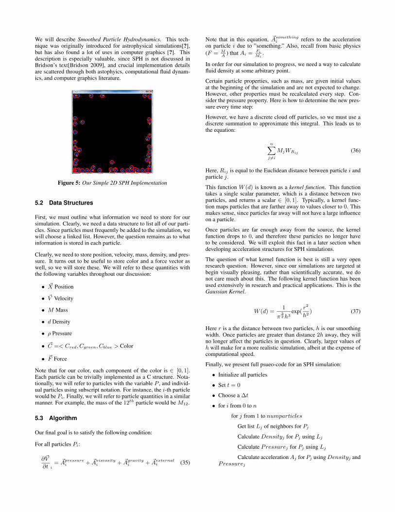
Figure 5: Our Simple 2D SPH Implementation

5.2 Data Structures

First, we must outline what information we need to store for oursimulation. Clearly, we need a data structure to list all of our parti-cles. Since particles must frequently be added to the simulation, wewill choose a linked list. However, the question remains as to whatinformation is stored in each particle.

Clearly, we need to store position, velocity, mass, density, and pres-sure. It turns out to be useful to store color and a force vector aswell, so we will store these. We will refer to these quantities withthe following variables throughout our discussion:

• ~X Position

• ~V Velocity

• M Mass

• d Density

• ρ Pressure

• ~C =< Cred, Cgreen, Cblue > Color

• ~F Force

Note that for our color, each component of the color is ∈ [0, 1].Each particle can be trivially implemented as a C structure. Nota-tionally, we will refer to particles with the variable P , and individ-ual particles using subscript notation. For instance, the i-th particlewould be Pi. Finally, we will refer to particle quantities in a similarmanner. For example, the mass of the 12th particle would be M12.

5.3 Algorithm

Our final goal is to satisfy the following condition:

For all particles Pi:

∂~V

∂t i= ~Apressure

i + ~Aviscosityi + ~Agravity

i + ~Aexternali (35)

Note that in this equation, ~Asomethingi refers to the acceleration

on particle i due to ”something.” Also, recall from basic physics(F = M

A) that Ai = Fi

Mi.

In order for our simulation to progress, we need a way to calculatefluid density at some arbitrary point.

Certain particle properties, such as mass, are given initial valuesat the beginning of the simulation and are not expected to change.However, other properties must be recalculated every step. Con-sider the pressure property. Here is how to determine the new pres-sure every time step:

However, we have a discrete cloud off particles, so we must use adiscrete summation to approximate this integral. This leads us tothe equation:

n∑j 6=i

MjWRij (36)

Here, Rij is equal to the Euclidean distance between particle i andparticle j.

This function W (d) is known as a kernel function. This functiontakes a single scalar parameter, which is a distance between twoparticles, and returns a scalar ∈ [0, 1]. Typically, a kernel func-tion maps particles that are farther away to values closer to 0. Thismakes sense, since particles far away will not have a large influenceon a particle.

Once particles are far enough away from the source, the kernelfunction drops to 0, and therefore these particles no longer haveto be considered. We will exploit this fact in a later section whendeveloping acceleration structures for SPH simulations.

The question of what kernel function is best is still a very openresearch question. However, since our simulations are targeted atbegin visually pleasing, rather than scientifically accurate, we donot care much about this. The following kernel function has beenused extensively in research and practical applications. This is theGaussian Kernel.

W (d) =1

π32 h3

exp(r2

h2) (37)

Here r is a the distance between two particles, h is our smoothingwidth. Once particles are greater than distance 2h away, they willno longer affect the particles in question. Clearly, larger values ofh will make for a more realistic simulation, albeit at the expense ofcomputational speed.

Finally, we present full psueo-code for an SPH simulation:

• Initialize all particles

• Set t = 0

• Choose a ∆t

• for i from 0 to n

for j from 1 to numparticles

Get list Lj of neighbors for Pj

Calculate Densityj for Pj using Lj

Calculate Pressurej for Pj using Lj

Calculate accelerationAj for Pj usingDensityj andPressurej

Move Pj using Aj and ∆t using Euler step

t = t+ ∆t

• Cleanup all data structures

• Exit

5.4 Acceleration Structures

As described above, there is a clear computational bottleneck in ourapplication. We must calculate interaction forces between each andevery particle. This is an O(n2) process, which is not computa-tionally viable. By using spatial data structures, we can reduce ourcomputation time to O(n) in the typical case. In the worst case,where all of the particles are in one cell, our algorithm still runsO(n2) Advanced techniques using quadtrees in 2D, or octrees in3D, can eliminate this possibility.

In addition to storing all of our particles in a linked list, we alsostore them in a spatial grid data structure. Our grid cells extendby a distance of R in each dimension. Therefore, in order to cal-culate the forces on a particular particle, one must only examine9 grid cells in the 2D case, or 27 grid cells in the 3D case. Thisis because, for any grid cells far enough away, our kernel functionwill evaluate to 0 and their contributions will not be included on thecurrent particle. In our experience, including this spatial grid candecrease simulation time by over an order of magnitude for largeenough simulations.

However, the addition of this grid data structure requires additionalbook-keeping during the simulation process. Whenever a particleis moved, one must remove it from its current grid cell, and add itto the grid cell it belongs in. Unfortunately, there is no way to dothis simulation in place, and one must maintain two copies of thesimulation grid.

Additionally, this fixed grid requires us to change our kernel func-tion. Oftentimes, implementors in graphics define their kernel func-tions using a piecewise function. If the particles are less than somedistance h apart, they evaluate some type of spline. If the particlesare farther away, the kernel instead evalutes to 0. However, moreadvanced kernels exist for these types of simulations, and they haverecently been used with success in graphics. One of the most com-mon advanced kernels is the cubic spline kernel.

Figure 6: Our 2D SPH Implementation with Lookup Grid

Finally, SPH can be further optimized in another way. SPH isclearly very data parallel. Therefore, each particle can be simu-lated in a separate thread with relative ease. Because of this, manyhigh performance SPH implementations are done on the GPU.

Figure 7: Raytraced GPU Based 3D SPH from University of Tokyo

5.5 Surface Tracking

At our current stage, all SPH results in is an unorganized pointcloud of fluid particles. This is unacceptable for most applications.Usually the compuiter graphics practitioner desires a way to renderthese fluids using a off-the-shelf 3D renderer. In this section, wewill outline a few techniques for transforming the result of our SPHsimulations into a renderable form.

T and probably the easiest technique, is to sample our SPH resultsonto a uniform grid. Here we can step through the uniform gridpoints, and sample the fluid density on these points. Then, we canuse this uniform grid as input to an application that performs iso-surface volume rendering. Here we have a choice between directvolume rendering, such as that presented in [Colin Braley 2009],and marching cubes[Lorenson and Cline 1982]. Direct volume ren-dering, typically done through volume raycasting, has the advan-tage of speed. However, there is no easy way to integrate this result-ing image with other generated images, and therefore this techniqueis only suitable for creating previews. Marching cubes, on the otherhand, produces triangle meshes. These meshes are suitable for usein a 3D animation program, and this is therefore a viable option forfinal production.

While there are benefits to sampling our SPH onto a grid, there areother techniques that often produce better results. Usually, thesetechniques use a special function for each particle that, whe com-bined with the other particles, produces a fluid surface.

The function usually used for this purpose was introduced by [Blinn1982]. This technique is often referred to as meta-balls or blobbiesin the graphics community.

F ( ~X) = Σni k(‖ ~X − ~xi‖

h) (38)

Where h is a user specified parameter representing the smooth-ness of the surface, and k is a kernel function like the one repre-sented above. Incremenetal improvements have been made to thethe above function throughout the years, the most imporortant ofwhich is presetned in [Williams 2008].

Figure 8: Metaball Based Surface Reconstruction

5.6 Extensions

This document has only scratched the surface in discussing the cur-rent state of the art fluid simulation techniques. For a thoroughexplanation of grid based methods, see [Bridson 2009]. No com-parable resource for SPH and particle based technique exists, butthe author recommends reading the papers of Nils Theurey, andthe SIGGRAPH 2006 Fluid Simulation Course Notes as a startingpoint.

Other active areas of fluid simulation research in the graphics com-munity include, smoke simulation, fire simulation, simulation ofhighly viscous fluids, and coupled simulations. Coupled simula-tions combine two or more simulations and get them to interactplausibly. Recently, Ron Fedkiw’s group achieved 2-way coupledSPH and grid based simulations in [?]. Furthermore, examples ofcouplings with thin shells, rigid body simulations, soft body simu-lations, and cloth simulations exist as well.

Figure 9: Two Way Coupled SPH and Grid Based Simulation byRon Fedkiw’s Group

Acknowledgments

Thanks to Robert Hagan for editing this work.

References

BATTY, C., AND BRIDSON, R. 2008. Accurate viscous free sur-faces for buckling, coiling, and rotating liquids. In Proceedingsof the 2008 ACM/Eurographics Symposium on Computer Ani-mation, 219–228.

BATTY, C., BERTAILS, F., AND BRIDSON, R. 2007. A fast varia-tional framework for accurate solid-fluid coupling. ACM Trans.Graph. 26, 3, 100.

BLINN, J. F. 1982. A generalization of algebraic surface drawing.ACM Trans. Graph. 1, 3, 235–256.

BRIDSON, R. 2009. Fluid Simulation For Computer Graphics.A.K Peters.

COLIN BRALEY, ROBERT HAGAN, Y. C. D. G. 2009. Gpu basedisosurface volume rendering using depth based coherence. Sig-graph Asia Technical Sketches.

FEDKIW, R., AND SETHIAN, J. 2002. Level Set Methods for Dy-namic and Implicit Surfaces.

FEDKIW, R., STAM, J., AND JENSEN, H. W. 2001. Visual sim-ulation of smoke. In Proceedings of SIGGRAPH 2001, ACMPress / ACM SIGGRAPH, E. Fiume, Ed., Computer GraphicsProceedings, Annual Conference Series, ACM, 15–22.

FEDKIW, R., STAM, J., AND JENSEN, H. W., 2001. Visual simu-lation of smoke.

FOSTER, N., AND FEDKIW, R. 2001. Practical animation of liq-uids. In SIGGRAPH ’01: Proceedings of the 28th annual con-ference on Computer graphics and interactive techniques, ACMPress, New York, NY, USA, 23–30.

GOKTEKIN, T. G., BARGTEIL, A. W., AND O’BRIEN, J. F. 2004.A method for animating viscoelastic fluids. ACM Transactionson Graphics (Proc. of ACM SIGGRAPH 2004) 23, 3, 463–468.

GUENDELMAN, E., SELLE, A., LOSASSO, F., AND FEDKIW, R.2005. Coupling water and smoke to thin deformable and rigidshells. In SIGGRAPH ’05: ACM SIGGRAPH 2005 Papers,ACM, New York, NY, USA, 973–981.

HARLOW, F., AND WELCH, J., 1965. Numerical calculation oftime-dependent viscous incompressible flow of fluid with a freesurface. the physics of fluids 8.

HARLOW, F., AND WELCH, J., 1965. Numerical calculation oftime-dependent viscous incompressible flow of fluid with a freesurface. the physics of fluids 8.

HARLOW, F., AND WELCH, J., 1965. Numerical calculation oftime-dependent viscous incompressible flow of fluid with a freesurface. the physics of fluids 8.

LORENSON, AND CLINE. 1982. Marching cubes. ACM Trans.Graph. 1, 3, 235–256.

PETER, M. C., MUCHA, P. J., BROOKS, R., III, V. H., ANDTURK, G., 2002. Melting and flowing.

PETER, M. C., MUCHA, P. J., AND TURK, G. 2004. Rigid fluid:Animating the interplay between rigid bodies and fluid. In ACMTrans. Graph, 377–384.

SETHIAN, J. A. 1999. Level Set Methods and Fast Marching Meth-ods: Evolving Interfaces in Computational Geometry, Fluid Me-chanics, Computer Vision, and Materials Science (Cambridge ...on Applied and Computational Mathematics), 2 ed. CambridgeUniversity Press, June.

SHEWCHUK, J. R. 2007. Conjugate gradient without the agonizingpain. Tech. rep., Carnegie Mellon.

STAM, J. 1999. Stable fluids. 121–128.

WILLIAMS, B. W. 2008. Fluid Surface Reconstruction from Par-ticles. Master’s thesis, University of British Columbia.