fluid stru ture intera tion - diva portal
TRANSCRIPT

FLUID-STRUCTURE INTERACTION EFFECTS OF SLOSHING IN LIQUID-CONTAINING STRUCTURES
KTH Royal Institute of Technology School of Architecture and the Built Environment
Infrastructure Engineering
March 2013 TRITA-BKN. Master Thesis 379, 2013
ISSN 1103-4297 ISRN KTH/BKN/EX-379-SE
Paul THIRIAT

1 Introduction
ABSTRACT This report presents the work done within the framework of my master thesis in the program Infrastructure
Engineering at KTH Royal Institute of Technology, Stockholm. This project has been proposed and sponsored by the
French company Setec TPI, part of the Setec group, located in Paris.
The overall goal of this study is to investigate fluid-structure interaction1 and particularly sloshing in liquid-
containing structures subjected to seismic or other dynamic action. After a brief introduction, the report is
composed of three main chapters. The first one presents and explains fluid-structure interaction equations. Fluid-
structure interaction problems obey a general flow equation and several boundary conditions, given some basic
assumptions. The purpose of the two following chapters is to solve the corresponding system of equations. The first
approach proposes an analytical solution: the problem is solved for 2D rectangular tanks. Different models are
considered and compared in order to analyze and describe sloshing phenomenon. Liquid can be decomposed in
two parts: the lower part that moves in unison with the structure is modeled as an impulsive added mass; the
upper part that sloshes is modeled as a convective added mass. Each of these two added mass creates
hydrodynamic pressures and simple formulas are given in order to compute them. The second approach proposes a
numerical solution: the goal is to be able to solve the problem for any kind of geometry. The differential problem is
resolved using a singularity method and Gauss functions. It is stated as a boundary integral equation and solved by
means of the Boundary Element Method. The linear system obtained is then implemented on Matlab. Scripts and
results are presented. Matlab programs are run to solve fluid-structure interaction problems in the case of
rectangular tanks: the results concur with the analytical solution which justifies the numerical solution.
This report gives a good introduction to sloshing phenomenon and gathers several analytical solutions found in the
literature. Besides, it provides a Matlab program able to model effects of sloshing in any liquid-containing
structures.
Keywords: fluid-structure interaction, sloshing, tank, seismic action, hydrodynamic pressure, velocity potential,
boundary element method, Housner, resonant sloshing
Author’s note: This version of the thesis, edited to be published on KTH Database, does not include the appendices
and Matlab scripts.
1 interaction of a movable structure with an internal or external fluid

2 Fluid-structure interaction
TABLE OF CONTENT 1 Introduction ........................................................................................................................................................... 7
2 Fluid-structure interaction ..................................................................................................................................... 8
2.1 Introduction ................................................................................................................................................... 8
2.2 Fluid equations ............................................................................................................................................... 8
2.2.1 Local equations ........................................................................................................................................ 8
2.2.2 Velocity potential ..................................................................................................................................... 9
2.3 Boundary conditions .................................................................................................................................... 10
2.3.1 Fluid-structure interface condition ........................................................................................................ 11
2.3.2 Free surface condition ............................................................................................................................ 11
2.3.3 Fluid-ground interface condition ........................................................................................................... 12
2.3.4 Inifite boundary condition ...................................................................................................................... 12
2.4 Conclusion .................................................................................................................................................... 13
3 Analytical solution for 2D rectangular tanks ........................................................................................................ 14
3.1 Introduction ................................................................................................................................................. 14
3.2 Problem presentation .................................................................................................................................. 15
3.2.1 Model and assumptions ......................................................................................................................... 15
3.2.2 Sloshing equations ................................................................................................................................. 16
3.3 Study of sloshing: time-history analysis ....................................................................................................... 17
3.3.1 Free oscillations ...................................................................................................................................... 17
3.3.2 Forced displacement .............................................................................................................................. 19
3.4 Resolution of the sloshing problem: frequency domain analysis ................................................................ 20
3.4.1 Steady state response: Graham & Rodriguez’s method ........................................................................ 20
3.4.1.1 Dynamic pressures acting on the tank walls ................................................................................. 21
3.4.1.2 Hydrodynamic forces ..................................................................................................................... 22
3.4.2 Transient and steady state response: Hunt & Priestley’s method ......................................................... 24

3 Introduction
3.4.2.1 Hydrodynamic pressures acting on the tank walls ........................................................................ 24
3.4.2.1.1 Hydrodynamic impulsive pressure ............................................................................................ 26
3.4.2.1.2 Hydrodynamic convective pressure .......................................................................................... 28
3.4.2.1.3 Interpretation ............................................................................................................................ 31
3.4.2.2 Hydrodynamic pressure forces ...................................................................................................... 31
3.4.2.2.1 Hydrodynamic impulsive pressure force ................................................................................... 31
3.4.2.2.2 Hydrodynamic convective pressure force ................................................................................. 32
3.4.2.3 Conclusion ..................................................................................................................................... 34
3.4.3 Housner’s approached method .............................................................................................................. 35
3.4.3.1 Impuslive part ................................................................................................................................ 36
3.4.3.2 Convective part.............................................................................................................................. 37
3.4.3.3 Model ............................................................................................................................................ 38
3.4.4 Conclusion .............................................................................................................................................. 38
3.5 Study of resonant sloshing ........................................................................................................................... 40
3.5.1 Resonant amplification .......................................................................................................................... 40
3.5.2 Frequency domain analysis .................................................................................................................... 45
3.5.3 Tuned sloshing dampers ........................................................................................................................ 48
3.5.4 Conclusion .............................................................................................................................................. 48
3.6 Conclusion .................................................................................................................................................... 50
4 Numerical solution for sloshing problems ........................................................................................................... 51
4.1 Introduction ................................................................................................................................................. 51
4.2 General method ........................................................................................................................................... 52
4.3 Singularity method ....................................................................................................................................... 54
4.3.1 Formulation ............................................................................................................................................ 54
4.3.1.1 Green indentities ........................................................................................................................... 54
4.3.1.2 Green function ............................................................................................................................... 54
4.3.1.3 Integral equation ........................................................................................................................... 54

4 Fluid-structure interaction
4.3.2 Solution: Boundary Element Method ..................................................................................................... 55
4.3.2.1 Green’s function for 2D problems ................................................................................................. 56
4.3.2.2 Green’s function for 3D problems ................................................................................................. 56
4.4 Examples and results .................................................................................................................................... 57
4.4.1 2D tanks .................................................................................................................................................. 57
4.4.1.1 Rectangular tanks .......................................................................................................................... 57
4.4.1.2 Circular tanks ................................................................................................................................. 61
4.4.2 3D tanks .................................................................................................................................................. 62
4.4.2.1 Internal problem ............................................................................................................................ 62
4.4.2.2 External problem ........................................................................................................................... 66
4.5 Conclusion .................................................................................................................................................... 67
5 General conclusion ............................................................................................................................................... 68

5 Introduction
TABLE OF FIGURES Figure 1: typical fluid-structure interaction problem ................................................................................................... 10
Figure 2: rectangular tank fixed to the ground ............................................................................................................ 15
Figure 3: rectangular tank fixed to the ground ............................................................................................................ 20
Figure 4: Graham & Rodriguez model – impulsive mass .............................................................................................. 23
Figure 5: Graham & Rodriguez's method - Impulsive mass ratio ................................................................................. 23
Figure 6: Hunt & Priestley's method - impulsive pressure at the bottom of the tank ................................................. 26
Figure 7: EN 1998-4 Figure A.6 - impulsive pressure at the bottom of the tank ......................................................... 27
Figure 8: Hunt & Priestley's method - Impulsive pressure ........................................................................................... 27
Figure 9: EN 1998-4 Figure A.7 - impulsive pressure ................................................................................................... 28
Figure 10: Hunt & Priestley's method - Convective pressure, sloshing mode 1 .......................................................... 29
Figure 11: Hunt & Priestley's method - Convective pressure, sloshing mode 2 .......................................................... 29
Figure 12: E EN 1998-4 Figure A.7 - convective pressure, sloshing mode 1 ................................................................. 30
Figure 13: EN 1998-4 Figure A.7 - convective pressure, sloshing mode 2 ................................................................... 30
Figure 14: Hunt & Priestley's method - Impulsive mass ratio for 1, 2, 3 and 10 sloshing modes ................................ 32
Figure 15: Hunt & Priestley's method – Convective mass ratio for the sloshing mode 1, 2 and 3 .............................. 33
Figure 16: Hunt & Priestley model – impulsive mass and convective mass (2 sloshing modes) ................................. 34
Figure 17: fundamental natural sloshing period for rectangular tanks ....................................................................... 35
Figure 18: Housner's method - lamina fluid theory ..................................................................................................... 36
Figure 19: Housner's method - Impulsive mass ratio, comparison with Graham & Rodriguez’s method ................... 36
Figure 20: Housner's method - Convective mass ratio, comparison with Hunt & Priestley's method ........................ 37
Figure 21: Housner's model - Impulsive and convective mass ..................................................................................... 38
Figure 22: resonant sloshing ........................................................................................................................................ 41
Figure 23: impulsive added mass for high frequencies as a function of L/h ................................................................ 42
Figure 24: resonant amplification coefficient as a function of L/h .............................................................................. 43
Figure 25: frequency window coefficient of the resonant amplification ..................................................................... 44

6 Fluid-structure interaction
Figure 26: natural sloshing frequency for different values of L ................................................................................... 44
Figure 27: resonant amplification ................................................................................................................................ 45
Figure 28: time-history recording – ground acceleration ............................................................................................ 45
Figure 29: frequency domain description – power spectral density ............................................................................ 46
Figure 30: rectangular tank fixed to the ground .......................................................................................................... 46
Figure 31: amplitude spectrum of the earthquake (blue) and the transfer function (green) ...................................... 47
Figure 32: inertia force caused by the seismic action .................................................................................................. 49
Figure 33: example of non-rectangular 2D tank .......................................................................................................... 51
Figure 34: problem geometry ...................................................................................................................................... 52
Figure 35: numerical and analytical added mass for 2D rectangular tanks ................................................................. 57
Figure 36: pressure distribution - vertical action ......................................................................................................... 58
Figure 37: pressure distribution - horizontal action ..................................................................................................... 58
Figure 38: pressure factor comparison of numerical and analytical solutions ............................................................ 59
Figure 39: horizontal added mass as a function of frequency ..................................................................................... 59
Figure 40: resonant sloshing for numerical and analytical solutions ........................................................................... 60
Figure 41: slosh2D convergence test ........................................................................................................................... 60
Figure 42: pressure distribution for a 2D circular pipe ................................................................................................ 61
Figure 43: pressure factor for 2D rectangular tank - Eurocode and numerical solution ............................................. 62
Figure 44: pressure acting on the walls for horizontal oscillation along x ................................................................... 63
Figure 45: pressure acting on the walls for horizontal oscillation along y ................................................................... 63
Figure 46: pressure acting on the walls for vertical oscillation .................................................................................... 64
Figure 47: added mass as a function of frequency for oscillation along x ................................................................... 64
Figure 48: added mass as a function of frequency for oscillation along y ................................................................... 65
Figure 49: slosh3D convergence test ........................................................................................................................... 65
Figure 50: external problem geometry ........................................................................................................................ 66
Figure 51: pressure factor on a dam - comparison of Westergaard's formula with numerical results ....................... 67

7 Introduction
1 INTRODUCTION
When subjected to external excitation like earthquake, liquid-containing structures are challenging to design due to
sloshing effects. Indeed, fluid-structure interaction is the source of free surface fluctuation and hydrodynamic
pressure loads that can cause unexpected instability or even failure of these structures. Thus, it is paramount to
carry out a thorough investigation about sloshing phenomenon. The main purpose of this report is to characterize
the dynamic response of liquid storage tanks.
In the first chapter of this study, equations that rule fluid-structure interaction are derived. The system to solve can
be summarized to a differential problem with boundary conditions, often called Dirichlet problem. Different
assumptions are discussed in order to obtain a simple model of the fluid behavior. Both analytical and numerical
methods are then proposed in order to solve this problem.
The first approach proposes an analytical solution: the problem is solved for 2D rectangular tanks. Different models
are considered and compared in order to analyze and describe sloshing phenomenon. This study is based on the
results found in the literature dealing with this subject. It is interesting to focus on rectangular tanks because they
represent the major part of practical cases. Besides, an analytical solution often provides a good understanding of
the general aspects ruling the phenomenon. A detailed investigation of resonant sloshing is also conducted in this
part.
The second approach proposes a numerical solution: the goal is to be able to solve the problem for any kind of
geometry. The differential problem is resolved using a singularity method and Gauss functions. It is stated as a
boundary integral equation and solved by means of the Boundary Element Method. Analytical and numerical
solutions are then compared and performance is discussed.
The whole study assumes that the mass of liquid is lumped on the wall, based on rigid wall boundary condition in
the calculation of hydrodynamic pressures. This assumption is widely used in practice, particularly for concrete
structures which have relatively high stiffness.
As a conclusion, several concepts that are not studied in detail in this paper are put into perspective. We can state
for example the development of Tuned Sloshing Dampers or the influence of flexible wall on the dynamic response
of liquid storage tanks.

8 Fluid-structure interaction
2 FLUID-STRUCTURE INTERACTION
2.1 INTRODUCTION
The goal of this chapter is to present and explain fluid-structure interaction equations. Fluid-structure interaction is
the interaction of a movable structure with an internal or external fluid.
In the first part, we will focus on the fluid. Different assumptions will be discussed in order to obtain a simple model
of the fluid behavior. We will demonstrate that, under certain conditions, the fluid obeys Laplace’s equation. It will
be done by considering the velocity potential function associated to the velocity field.
Then, in a second part, we will analyze several boundary conditions which are likely to occur in fluid-structure
interaction problems. In particular, we will present free surface and fluid-structure interface boundary conditions.
Finally, we will expose the system of equations to solve in order to model fluid-structure interaction.
2.2 FLUID EQUATIONS
In this part, we will derive the fundamental equations of the fluid. It will be done by writing local fluid equations.
Then these equations will be simplified thanks to basic assumptions.
2.2.1 LOCAL EQUATIONS
We consider a fluid domain Ω described, for each point of Ω, by the following local functions:
Its velocity field ;
Its density ;
Its hydrodynamic pressure .
Each function depends on space and time.
The fluid flow obeys two fundamental local equations of conservation:
Continuity equation, which expresses the conservation of mass [4]:
( )
Euler’s equation, which expresses the conservation of momentum [4]:
(
( ) ( ) ) ( )
In this last equation, represents body forces acting on the fluid, such as the gravity force for example. is the
stress tensor.
It is possible to assume that the flow is incompressible. Indeed, we study liquid with low flow velocity. This
property implies that the density is constant and homogeneous. From the continuity equation, we obtain the
well-known criterion of incompressibility:
( )

9 Fluid-structure interaction
The incompressible flow assumption is valid if [15]:
With
is the Strouhal number and
is the Mach number. In this study, we have and
. Thus, the above condition becomes:
The frequency range for seismic action is between 0 and 50 rad.s-1 so the incompressible flow assumption is valid.
The stress tensor can be expressed as a function of the pressure p, the viscosity and the strain gradient tensor
as follow [4]:
( ( ) ( ))
Euler’s equation can be simplified thanks to the perfect fluid model, which implies the following assumptions:
The fluid is assumed to be inviscid: ;
The flow is irrotational: ( ) .
Euler’s equation becomes Navier-Stokes equation:
(
( )) ( )
2.2.2 VELOCITY POTENTIAL
The assumption of irrotational flow implies that there is a velocity potential function that satisfies:
( )
If we now use the property of incompressibility, expressed in the previous part by:
( )
It yields that:
In the case of an irrotational and incompressible flow, the fluid can be represented by its velocity potential
function, which satisfies Laplace’s equation.
If we now consider a compressible flow, we can show that the velocity potential function verifies Helmholtz
equation [6]:

10 Fluid-structure interaction
This is the wave equation that expresses the pressure propagation in the fluid (with c the velocity of the sound in
the fluid). When we use Laplace’s equation, we consider that this propagation is instantaneous. This assumption is
correct when the velocity c is high before the dimension of the problem. It is the case for the study of water
sloshing in tanks for example.
Body forces derive from a potential. For example, gravity field force gives ( ). Thus, Navier-
Stokes’ equation becomes:
(
)
After integration of this equation in the fluid domain, we get Bernoulli’s equation:
( )
Fluid-structure interaction problems always consider small displacement. Thus, it is possible to neglect . It is
possible to “include” the time-dependent function k in the velocity potential (we still have ( )because
( ) ) and we finally obtain linearized Lagrange’s equation where p is the total pressure (sum of the
hydrodynamic and hydrostatic pressure):
This formula is paramount because we want to represent the fluid-structure interaction by the velocity potential
function. So it will allow us to compute the value of the pressure with the knowledge of the velocity potential.
2.3 BOUNDARY CONDITIONS
Now that we have derived the equations that describe the fluid behavior (in particular Laplace’s equation), we
need to express boundary conditions in order to solve fluid-structure interaction problems. A typical and general
fluid-structure interaction problem is depicted below (Figure 1).
Figure 1: typical fluid-structure interaction problem
Ground
Γi
Γg
Γs
Γfs
z
x
n
n
Structure
Fluid Ω

11 Fluid-structure interaction
We can distinguish 4 borders:
Γs represents the interface between structure and fluid;
Γsf represents the free surface;
Γg represents the interface between ground and fluid;
Γi is an imaginary boundary to model an “infinite” domain of water.
We have the following properties:
Fluid density:
Sound velocity in the fluid: c
Ground density:
Sound velocity in the ground: cg
This figure can describe, for example, a dam. In this case, it is of great important to be able to model fluid-structure
interaction when a seismic action occurs in order to assess the response of the structure. The velocity of the ground
due to the seismic action is .
2.3.1 FLUID-STRUCTURE INTERFACE CONDITION
The structure is animated by a movement . We want to express the continuity between the velocity field in the
fluid and the loads in the structure. At the fluid-structure interface, if we consider a fluid and a solid particle, the
normal velocity will be equal, so it holds that [3]:
This condition can be expressed in terms of velocity potential. With ( )
, it holds that:
is the velocity of the structure’s particles at the fluid-structure interface. In the case of a rigid structure, this
velocity is equal to the ground velocity which is known. However, if we have a deformable structure, we have to
add the velocity due to structure deformation and we get: . In this case, is unknown and we have
a coupled system.
2.3.2 FREE SURFACE CONDITION
Free surface condition can be expressed by the means of gravity waves. For each point of the free surface, the
pressure is given by the fluctuation of the vertical velocity field [3]:
In this formula, we can replace the pressure by its expression as a function of the velocity potential found in the
previous part.
Besides, by definition of the velocity potential function, we have:

12 Fluid-structure interaction
It is now possible to express the free surface condition with the velocity potential.
This condition allows us to study waves and surface fluctuation. In particular, we need to know the waves’ height if
we want to avoid overflow. However, it is sometimes possible to take a simpler condition which does not involve
time. In fact, we consider only high frequency response (for seismic action for example), so it holds that [6]:
2.3.3 FLUID-GROUND INTERFACE CONDITION
The ground is made of poroelastic material and can absorb pressure waves. The damping factor of the ground
can be express as follow [8]:
And the fluid-ground interaction condition is given by [8]:
Of course, in the case of a rigid ground-water interface, and the condition is the same than the one for the
fluid-structure interface.
2.3.4 INIFITE BOUNDARY CONDITION
At this interface, we have to model waves’ propagation from the fluid-structure interface toward the other side of
the tank. We suppose that the tank is big enough so that there is no wave reflection. The most common condition
is called the Sommerfeld radiation condition [8]:
One has to be careful with the distance between the structure and the imaginary boundary. It is recommended to
choose a distance of at least 5h, h being the height of the wet structure.

13 Fluid-structure interaction
2.4 CONCLUSION
Basically, we can summarize fluid-structure interaction problems to the mathematical resolution of Laplace’s
equation with Neumann boundary conditons.
For a perfect fluid, it is convenient to model fluid-structure interaction with its velocity potential. Thus, we have the
following system of equations:
{
{
{
{
This kind of system of differential equation can be really challenging to solve. That is what is done in detail in the
following chapters of this paper.
The first approached presented is an analytical solution. It is doable for problems with simple geometries only. The
second one is a numerical solution that uses Boundary Elements Method and Gauss functions.

14 Fluid-structure interaction
3 ANALYTICAL SOLUTION FOR 2D RECTANGULAR TANKS
3.1 INTRODUCTION
In this chapter, we solve the fluid-structure interaction problem in the simple case of a 2D rectangular tank. The
starting point is the Neumann problem derived in the previous part. Thanks to the simple geometry, it is possible to
solve analytically the sloshing problem. Actually, an analytical solution is possible for rectangular and circular tanks
only. These kinds of tanks represent most practical cases, that is why it is useful to focus on them. Moreover, an
analytical solution will give us a good understanding of the solution we get at the end.
We are going to study fluid-structure interaction when some water, contained in a rectangular tank, is subjected to
an external action (a seismic action for example). During an earthquake, the mass of water contained in the
structure will move because of the displacement of the solid: that is what we call “sloshing”.
Water sloshing induces hydrodynamic (or fluctuating) pressures on the vertical tank walls because of the horizontal
acceleration of the structure. The goal of this study is to assess the value of these hydrodynamic loads.
The simplest way to compute the horizontal pressure forces when the tank is subjected to a seismic action,
represented by horizontal ground acceleration, is to “accelerate” the whole mass of water as if it were acting like a
rigid body. Therefore, the hydrodynamic forces will be proportional to the total mass of water. However, the water
does not behave like a rigid body: it is a conservative assumption that is way too detrimental to structure design.
That is why we have to model the fluid flow and the interaction between the fluid and the solid that are both
moving.
The literature presents several methods in order to express the value of the fluctuating pressure [1]. This part
explains and details these different approaches and compares the assumptions and the results obtained. The whole
study assumes that the mass of liquid is lumped on the wall, based on rigid wall boundary condition in the
calculation of hydrodynamic pressures. This assumption is widely used in practice, particularly for concrete
structures which have relatively high stiffness.
In the first part, we will present the problem and give the system of equation to solve. We will explain the different
assumptions made. In the second part, we will study the sloshing phenomenon and the time-history response with
free and forced oscillations. Then, in the third part, we will solve the sloshing problem using several approaches.
The results will be compared to the one we can find in the literature (Eurocode 8.4 for example).

15 Analytical solution for 2D rectangular tanks
3.2 PROBLEM PRESENTATION
3.2.1 MODEL AND ASSUMPTIONS
The structure studied is modeled by a 2D rectangular tank fixed to the ground as depicted in the figure below
(Figure 2). The tank is subjected to a horizontal acceleration (ground acceleration due to seismic action for
example).
Figure 2: rectangular tank fixed to the ground
We define the dimensionless coefficient that describes the geometry of the system:
With:
L: inside length of the tank, in meter;
h: height of water in the tank, in meter.
The density of the water, expressed in t.m-3, is noted . Thus, the mass of water is: , in
is the horizontal displacement of the structure, in meter. The acceleration of gravity is noted g.
We assume that the fluid has the following properties:
Incompressible fluid;
Inviscid flow;
Small displacement;
Non-turbulent regime;
Irrotational flow.
These are the usual assumptions for a perfect fluid. These assumptions are realistic in the case of water contained
in a tank and they will allow us to solve analytically the problem.
We define everywhere in the fluid:
( ) ( ) ( ) : velocity of the fluid;
( ): pressure in the fluid.
L/2
h
Xs
ex (0; 0)

16 Fluid-structure interaction
3.2.2 SLOSHING EQUATIONS
Given the assumptions, the velocity potential function verifies Laplace’s equation (see previous part):
( )
In this case, we have two types of “boundary” conditions: free surface and fluid-structure interface.
With the gravity wave theory, the free surface condition is:
( )
( )
We have a minus sign because the z-axis is downward pointing.
The movement is horizontal, so given the tank’s geometry we have simple fluid-structure boundary conditions:
{
(
) ( )
(
) ( )
( )
The first two conditions describe the interface with the edges of the tank (x = -L/2 and x = L/2). The last one is the
condition at the bottom (z = h).
The problem to solve is described by the following equations which are respectively Laplace’s equation, the free
surface condition and the boundary fluid-solid interface conditions:
{
( )
( )
( )
{
(
) ( )
(
) ( )
( )
The flow is described by the fluid’s velocity potential.

17 Analytical solution for 2D rectangular tanks
3.3 STUDY OF SLOSHING: TIME-HISTORY ANALYSIS
3.3.1 FREE OSCILLATIONS
In this part, we are looking for the sloshing modes in the case of free oscillations. It means that:
( )
So the problem to solve becomes:
{
( )
( )
( )
{
(
)
(
)
( )
This system is going to be solved with a modal decomposition of the velocity potential. So we are looking for
solution of this type:
( ) ( ) ( )
We are looking for decoupled solutions, that is to say:
( ) ( ) ( )
The modal function verifies:
( )
So it yields:
(
) ( ) (
) ( )
The functions cos, sin, sh and ch are the solutions of this equation. a and b have the same “frequency”.
The interface conditions gives:
{ (
)
(
)
( )
The 2 first conditions give the expression of a:
(
(
))

18 Fluid-structure interaction
And the last one gives b:
(
( ))
We can choose A = B = 1 and we have:
( ) (
(
)) (
( ))
The free surface condition becomes:
( )
( )
( ) ( )
This is the equation of a harmonic oscillator without damping. It implies that is a sinusoidal function whose
frequency satisfies:
( )
( )
And we find:
{
( ) ( )
(
)
n is sloshing mode of the fluid in the tank. The solution of the free oscillation problem is the sum of the contribution of every sloshing mode:
( ) ∑ ( ) ( )
And we know the fundamental sloshing frequency for a rectangular tank:
√
(
)
The shallower the tank is, the smaller the natural sloshing frequency is.

19 Analytical solution for 2D rectangular tanks
3.3.2 FORCED DISPLACEMENT
In this part, we consider that the tank is subjected to a horizontal displacement .
We suppose that the family of modal functions ( ) found previously forms a basis of functions of [
]
[ ]. This is an orthogonal family for the usual inner product. We are looking for a velocity field of this type:
( ) ∑ ( ) ( )
( )
With:
( ) (
(
)) (
( ))
So ( ) verifies the following system of equations:
{
( )
( )
( )
{
(
) ( )
(
) ( )
( )
So is solution of the sloshing problem.
The projection of the free surface condition on the n sloshing modes (which are orthogonal) gives n equations:
[∫ ( )
] ( ) [ ∫
( ) ( )
] ( ) [ ∫ ( )
] ( )
After calculation, we obtain n equations of oscillators:
( ) ( ) ( ) ( )
With:
{
(
)
( )
( )
(
)
Each equation describes one sloshing mode.
Now, it is possible to compute the time-history seismic response of a rectangular tank containing liquid with the
knowledge of an accelerogram of an earthquake. Indeed, the accelerogram gives the input value and it is
possible to solve ( ) for every time step and every sloshing mode.
20 Fluid-structure interaction
3.4 RESOLUTION OF THE SLOSHING PROBLEM: FREQUENCY DOMAIN ANALYSIS
We still consider the 2D rectangular tank fixed to the ground (Figure 3):
Figure 3: rectangular tank fixed to the ground
This part proposes frequency-domain based solutions. Thus, the imposed displacement is a harmonic oscillation
along ex:
( )
( )
The frequency-domain based resolution will not give us access to the time response of the system but we will get
the maximum deformation (and loads) induced by a given elastic ground acceleration response spectrum.
The problem is going to be solved using different method. In the first one, we neglect the transient state. We find
the results proposed by Graham & Rodriguez [1]: the fluid is assimilated to an equivalent impulsive added mass
that moves in unison with the tank. In a second part, when we take into account the transient state, an oscillating
mass is added to the model: this is equivalent to the solution proposed by Hunt & Priestley [1]. The results are then
compared with the one given in the Eurocode 8.4 [2]. And finally, we take a look at Housner’s method [1], which is
an approached method that gives simple expressions for the added impulsive and oscillating masses. In the
conclusion of this part, the results are compared and the differences are explained.
3.4.1 STEADY STATE RESPONSE: GRAHAM & RODRIGUEZ’S METHOD
In this method, we neglect the transient state. So the differential equations ( ) found in the previous part can be
easily solved by finding a particular integral of the problem (by using a complex resolution for example):
( )
(
) ( )
And we have:
( ) ( )
So when we consider only the steady state of the response of the tank due to harmonic oscillations, ( ) is given
by:
L/2
h
Xs
ex (0; 0)
21 Analytical solution for 2D rectangular tanks
( )
(
) ( )
And we get the expression of the velocity field:
( ) [∑ (
(
)) (
( ))
(
) ] ( )
With:
{
(
)
( )
( )
(
)
3.4.1.1 DYNAMIC PRESSURES ACTING ON THE TANK WALLS
Now we can express the value of the pressure, given by the usual formula:
( )
( )
And we find:
( ) [∑ (
(
)) (
( ))
(
) ] ( )
The expression of the pressure gives access to the pressure factor ( ) on the vertical tank wall (for x= L/2)
defined by:
(
) ( ) ( )
So we it yields:
( ) [∑( ) (
( ))
(
)
]
The seismic action has a huge importance for high frequencies. Besides, we will prove later that we only have to
take into account the first sloshing modes (so low frequency modes) to have a good estimate of sloshing effects.
Thus, we can consider that:
(
)
This assumption will be discussed afterward in the part “Study of resonant sloshing”.

22 Fluid-structure interaction
And the pressure factor becomes:
( )
[
∑
(( )
( ))
(( ) ) (
( )
)
]
3.4.1.2 HYDRODYNAMIC FORCES
What we want is the value of the force caused by this fluctuating pressure on the vertical tank walls. Thus, we
integrate the expression of the pressure on the wall (from z = 0 to h) and we compute the value for x = L/2.
( ) ∫ (
)
We have to multiply by 2 because the pressure is acting on the 2 vertical tank walls.
And we find the hydrodynamic pressure force on the vertical tank wall:
( ) [ ∑ (( )
)
( )
(
)
] ( )
With:
( )
(( )
)
The value of the horizontal pressure force applied on the vertical tank wall can be written:
( ) ( ) ( )
With:
( ) [ ∑ (( )
)
( )
(
)
]
This expression represents the virtual mass of water which exerts a force on the structure when subjected to a
harmonic solicitation of frequency ω. The force caused by this mass and proportional to the acceleration ( )
is called the impulsive force.
It proves that it is not necessary to take the whole mass of water contained in the tank ( ), but we just
need to consider a certain ratio of this mass. This is due to the interaction between the fluid and the structure. So
finally, it is possible to model the phenomenon of sloshing in the tank by replacing the water by the added
impulsive mass mi.
Therefore, it is possible to see the system as depicted in the Figure 4:

23 Analytical solution for 2D rectangular tanks
Figure 4: Graham & Rodriguez model – impulsive mass
The resonance aspects will be studied afterward.
We can express the ratio
as a function of the dimensionless coefficient
⁄ for high oscillation frequencies
(i.e. (
)
):
∑
(( )
)
( )
The abacus that gives the percentage of impulsive mass to take into account for the calculation is presented below (Figure 5):
Figure 5: Graham & Rodriguez's method - Impulsive mass ratio
0
0,1
0,2
0,3
0,4
0,5
0,6
0,7
0,8
0,9
1
0 1 2 3 4 5 6 7 8 9 10
mi/
mw
α = L/h
Impulsive mass ratio
L
hi
Xs
ex
ez
mi

24 Fluid-structure interaction
3.4.2 TRANSIENT AND STEADY STATE RESPONSE: HUNT & PRIESTLEY’S METHOD
In this part, we do not neglect the transient part of the solution. So we want the exact solutions of the differential
equations ( ) which are given by Duhamel’s equation:
( )
∫ ( )
( ( ))
This equation is valid because we can assume that the system is initially at rest. That gives initials conditions:
{ ( )
( )
We are still studying the case of harmonic oscillations:
( )
( )
The solution is the sum of a particular and a general solution of the differential equation, which leads to:
( )
(
) ( ( ) ( ))
So we have the expression of the velocity field:
( ) [∑ (
(
)) (
( ))
(
) ] ( )
∑ (
(
)) (
( ))
(
) ( )
With:
{
(
)
( )
( )
(
)
3.4.2.1 HYDRODYNAMIC PRESSURES ACTING ON THE TANK WALLS
Now we can express the value of the pressure, which is given by:
( )
( )
It holds that:

25 Analytical solution for 2D rectangular tanks
( ) [∑ (
(
)) (
( ))
(
) ] ( )
∑ (
(
)) (
( ))
(
) ( )
The hydrodynamic pressure consists of two terms; one proportional to the acceleration of the structure ( ), the other is proportional to ( ) for each element of the sum (i.e. for each sloshing mode).
Actually, if we compare this result to the one of Graham & Rodriguez’s method, we note that the term that is
proportional to ( ) is the pressure factor ( ) on the vertical tank wall (for x= L/2) found previously. This is the
impulsive pressure.
( ) ( ) ( )
With the impulsive pressure factor:
( ) [∑( ) (
( ))
(
)
]
The only difference with Graham & Rodriguez’s method is the presence of an oscillating term. For each mode, we have an oscillating hydrodynamic pressure with a frequency equal to the natural sloshing frequency of this mode. This is the convective pressure defined for each sloshing mode:
( )
( ) ( )
With the convective pressure factor on the vertical tank wall (for x= L/2):
( ) ( ) (
( ))
(
)
And the oscillating acceleration:
( ) ( )
Finally, the total hydrodynamic pressure can be written:
( ) ( ) ∑ ( )
It is possible to compare this expression with the abacus that we find in the Eurocode. It is however necessary to be
careful with the notations. Indeed, the Eurocode considers a tank with a width of 2L and z = 0 corresponds to the
bottom of the tank (while z = h corresponds to the free surface).
Let’s use these notations, that we write L’ and z’ (for the half width and the new vertical coordinate).
In the Eurocode, the dimensionless parameter used is:

26 Fluid-structure interaction
Besides, the results presented in the Eurocode consider only high frequencies, so:
(
)
3.4.2.1.1 HYDRODYNAMIC IMPULSIVE PRESSURE
In the Eurocode, the impulsive pressure is given by:
( ) ( ) ( )
Where ( ) is the ground acceleration.
Thus, we get the expression of the dimensionless impulsive pressure as a function of and
:
(
) ∑
(( )
)
(( ) ) (
( )
)
Now, we can draw the graph that represents ( )as a function of (Figure 6). Here, z’ = 0 represents the bottom
of the tank.
Figure 6: Hunt & Priestley's method - impulsive pressure at the bottom of the tank
0
0,2
0,4
0,6
0,8
1
0 1 2 3 4 5
q0(0
)
β = h/L'
Dimensionless impulsive pressure at the bottom of the tank

27 Analytical solution for 2D rectangular tanks
The abacus given by the Eurocode [2] is presented below (Figure 7):
Figure 7: EN 1998-4 Figure A.6 - impulsive pressure at the bottom of the tank
We can also draw the graph that gives the ratio (
)
( )⁄ as a function of ⁄ for several value of
⁄ . This
graph (Figure 8) represents the shape of the impulsive hydrodynamic pressure along the vertical wall of the tank.
Figure 8: Hunt & Priestley's method - Impulsive pressure
0
0,2
0,4
0,6
0,8
1
0 0,2 0,4 0,6 0,8 1
z'/h
q0(z'/h)/q0(0)
Dimensionless impulsive pressure
h/L' = 0.1
h/L' = 1
h/L' = 3
h/L' = 5

28 Fluid-structure interaction
The abacus given by the Eurocode [2] is presented below (Figure 9):
Figure 9: EN 1998-4 Figure A.7 - impulsive pressure
3.4.2.1.2 HYDRODYNAMIC CONVECTIVE PRESSURE
In the Eurocode, the impulsive pressure is given by:
( )
( ) ( )
Where ( ) is the acceleration response function of a simple oscillator having frequency of the n mode.
Thus, we get the expression of the dimensionless impulsive pressure as a function of and
:
(
)
(( )
)
(( ) ) (
( )
)
We can now draw the hydrodynamic convective pressure for the first and second sloshing mode and for different
value of (Figure 10 and Figure 11). These graphs represent the shape of the convective hydrodynamic pressure
along the vertical wall of the tank.

29 Analytical solution for 2D rectangular tanks
Figure 10: Hunt & Priestley's method - Convective pressure, sloshing mode 1
Figure 11: Hunt & Priestley's method - Convective pressure, sloshing mode 2
0
0,2
0,4
0,6
0,8
1
0 0,2 0,4 0,6 0,8
z'/h
qc1(z'/h)
Dimensionless convective pressure: sloshing mode 1
h/L' = 0.3
h/L' = 0.5
h/L' = 1
h/L' = 2
h/L' = 5
0
0,2
0,4
0,6
0,8
1
0 0,02 0,04 0,06 0,08
z'/h
qc2(z'/h)
Dimensionless convective pressure: sloshing mode 2
h/L' = 0.3
h/L' = 0.5
h/L' = 1
h/L' = 2
h/L' = 5

30 Fluid-structure interaction
The abacuses given by the Eurocode [2] are presented below (Figure 12 and Figure 13):
Figure 12: E EN 1998-4 Figure A.7 - convective pressure, sloshing mode 1
Figure 13: EN 1998-4 Figure A.7 - convective pressure, sloshing mode 2

31 Analytical solution for 2D rectangular tanks
3.4.2.1.3 INTERPRETATION
The different graphs depicted in the previous part give results in accordance with the Eurocode. The work done in
this study gives analytical expressions for the impulsive and convective pressures. These formulas are much more
accurate and easier to use than the abacus proposed by the Eurocode.
3.4.2.2 HYDRODYNAMIC PRESSURE FORCES
What we want is the value of the force caused by this fluctuating pressure on the vertical tank walls. Thus, we
integrate the expression of the pressure on the vertical wall (from z = 0 to h) and we compute the value for x = L/2.
( ) ∫ (
)
We have to multiply by 2 because the pressure is acting on the 2 vertical canal-bridge walls.
And we find:
( )
[
∑
(( )
)
( )
(
)
]
( )
∑
(( )
)
( )
(
)
( )
With:
( )
(( )
)
The transverse force consists of two terms; one proportional to the acceleration of the structure ( ), the other is proportional to ( ) for each element of the sum (i.e. for each sloshing mode).
3.4.2.2.1 HYDRODYNAMIC IMPULSIVE PRESSURE FORCE
Actually, if we compare this result to the one of Graham & Rodriguez’s method, we note that the term that is
proportional to ( ) is the impulsive added mass found previously: it is the impulsive pressure force.
( ) ( ) ( )
With:
( ) [ ∑ (( )
)
( )
(
)
]
32 Fluid-structure interaction
We can express the ratio
as a function of the dimensionless coefficient
⁄ for high frequencies (i.e.
(
)
):
∑
(( )
)
( )
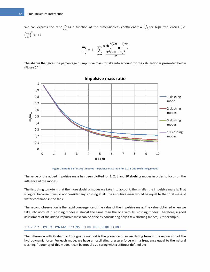
The abacus that gives the percentage of impulsive mass to take into account for the calculation is presented below (Figure 14):
Figure 14: Hunt & Priestley's method - Impulsive mass ratio for 1, 2, 3 and 10 sloshing modes
The value of the added impulsive mass has been plotted for 1, 2, 3 and 10 sloshing modes in order to focus on the
influence of the modes.
The first thing to note is that the more sloshing modes we take into account, the smaller the impulsive mass is. That
is logical because if we do not consider any sloshing at all, the impulsive mass would be equal to the total mass of
water contained in the tank.
The second observation is the rapid convergence of the value of the impulsive mass. The value obtained when we
take into account 3 sloshing modes is almost the same than the one with 10 sloshing modes. Therefore, a good
assessment of the added impulsive mass can be done by considering only a few sloshing modes, 3 for example.
3.4.2.2.2 HYDRODYNAMIC CONVECTIVE PRESSURE FORCE
The difference with Graham & Rodriguez’s method is the presence of an oscillating term in the expression of the hydrodynamic force. For each mode, we have an oscillating pressure force with a frequency equal to the natural sloshing frequency of this mode. It can be model as a spring with a stiffness defined by:
0
0,1
0,2
0,3
0,4
0,5
0,6
0,7
0,8
0,9
1
0 1 2 3 4 5 6 7 8 9 10
mi/
mw
α = L/h
Impulsive mass ratio
1 sloshingmode
2 sloshingmodes
3 sloshingmodes
10 sloshingmodes

33 Analytical solution for 2D rectangular tanks
With the added convective mass of water (with an oscillating movement ( )
( )) given
by:
[ (( )
)
( )
(
)
]
And the natural frequency of the sloshing mode n:
( )
(( )
)
It is the convective force:
∑
( )
We can express the ratio
as a function of the dimensionless coefficient
⁄ for high frequencies (i.e.
(
)
):
(( )
)
( )
Depicted below is the convective mass ratio for the first 3 sloshing modes (Figure 15).
Figure 15: Hunt & Priestley's method – Convective mass ratio for the sloshing mode 1, 2 and 3
0
0,1
0,2
0,3
0,4
0,5
0,6
0,7
0,8
0,9
1
0 1 2 3 4 5 6 7 8 9 10
mc,
n/m
w
α = L/h
Convective mass ratio
Sloshingmode 1Sloshingmode 2Sloshingmode 3

34 Fluid-structure interaction
Once again, what stands out of this graph is the small contribution of the modes other than the fundamental mode.
A good assessment of the convective force can be obtained by taking into account a few sloshing modes, like the
first and second one for example.
3.4.2.3 CONCLUSION
For high frequencies, Hunt & Priestley’s method decomposes the horizontal pressure force into two distinct parts:
An impulsive force, the same than the one proposed by Graham & Rodriguez, which represents the ratio of water that moves in unison with the tank:
( )
An convective force, which is the sum of the oscillation of every sloshing modes:
∑
( )
The only difference with the previous approach is that the solution of the differential equation is composed of the general solution and a particular solution. That’s why we have the convective forces, which stand for the “transient state” of the response. And the hydrodynamic pressure force can be written as the contribution of these two forces:
Therefore, it is possible to model the system as depicted in the Figure 16. It is important to remember that this
mechanical analogy is only possible when we consider that the added masses are independent of the oscillation
frequency (i.e. for high frequencies compared to natural sloshing frequencies).
Figure 16: Hunt & Priestley model – impulsive mass and convective mass (2 sloshing modes)
The graphs that give the values of the impulsive and convective hydrodynamic pressures prove that the impulsive
mass is mainly acting on the lower part of the tank while the added convective masses are mainly acting on the
upper part of the tank. Indeed, the waves that cause the convective forces are developed on the surface of the
fluid.
Besides, the graphs that give the values of the added impulsive and convective mass show that the shallower the
tank is, the more important the convective forces are (it is the opposite for the impulsive mass). Once again, that
can be explained by the fact that the waves that cause the convective forces are developed on the surface of the
mi
mc,1
mc,2
ex
ez ko,1/2
ko,1
/2
ko,2
/2 ko,2
/2
Xs
Xo,2
Xo,1

35 Analytical solution for 2D rectangular tanks
fluid: their influence will be even more important than these waves represent a large part of the fluid. This is the
case for shallow tanks.
In a practical case, it will be interesting to compare the impulsive and convective forces. In particular, is it possible
to neglect one of them? When we look at the fundamental natural sloshing frequency of water for different tank
geometry, we get the following graph (Figure 17):
Figure 17: fundamental natural sloshing period for rectangular tanks
The fundamental period of water sloshing is, for most of the cases, several seconds long. At such long periods, the
generated hydrodynamic convective pressures are much smaller than the hydrodynamic impulsive pressures. The
convective forces are generally negligible and can be ignored [9]. It is however necessary to be careful when L is
small (less than 5m) even if the failure risks when an earthquake occurs for such a small tank are not very high.
Besides, we know that the added convective mass ratio is important for shallow tanks, so when L is large in
comparison with h.
3.4.3 HOUSNER’S APPROACHED METHOD
Housner’s method is a widely used approach to assess sloshing effects in a tank containing a liquid during an
earthquake. The principle of this approach is based on the movement of the fluid. When the tank is subjected to a
horizontal acceleration, a part of the water moves together with the tank walls: the pressure force caused by this
1
5
913
1721
2529
02468
101214161820
15
9
L (m)
Fun
dam
en
tal s
losh
ing
pe
rio
d T
(s)
h (m)
Fundamental natural sloshing periods as a function of the tank dimensions
18-20
16-18
14-16
12-14
10-12
8-10
6-8
4-6
1
5
9
1 3 5 7 9 11 13 15 17 19 21 23 25 27 29 L (m)
h (m)
18-2016-1814-1612-1410-128-106-84-62-40-2

36 Fluid-structure interaction
movement is proportional to the acceleration of the tank. Besides, the upper part of the fluid starts to slosh and
causes vibration forces on the tank walls.
Actually, this description of the fluid movement corresponds to the expression of the pressure forces found in the
previous part with Hunt & Priestley’s method. Housner used the lamina fluid theory to calculate the impulsive and
convective hydrodynamic pressure [1]. The liquid is assumed to be incompressible and undergo small
displacements.
Figure 18: Housner's method - lamina fluid theory
Housner’s method is an approximate method that gives simple expressions for the impulsive and convective
masses mi and mc.
3.4.3.1 IMPUSLIVE PART
The value of the added impulsive mass is given by [1]:
(√
)
√
We can express the ratio
as a function of the dimensionless coefficient
⁄ . The abacus that gives the
percentage of added impulsive mass to take into account for the calculation is presented below (Figure 19). The
results of Housner’s method are compared with the results of Graham & Rodriguez’s method.
Figure 19: Housner's method - Impulsive mass ratio, comparison with Graham & Rodriguez’s method
00,10,20,30,40,50,60,70,80,9
1
0 1 2 3 4 5 6 7 8 9 10
mi/
mw
α = L/h
Impulsive mass ratio
Housner
u(x,t)
L
dx
h

37 Analytical solution for 2D rectangular tanks
The result of the impulsive mass given by Housner is very close to the one obtained previously, in particular for
shallow tanks. For α < 2, it might be better to use Graham & Rodriguez’s method.
Housner method provides also a simple formula that gives the point of application of the resulting pressure force
[1]:
3.4.3.2 CONVECTIVE PART
This method considers only the first sloshing mode for the value of the added convective mass. We have
demonstrated previously that this is a valid assumption. This mass is given by [1]:
(√
)
We can express the ratio
as a function of the dimensionless coefficient
⁄ . The abacus that gives the
percentage of added convective mass to take into account for the calculation is presented below (Figure 20). The
results of Housner’s method are compared with the results of Hunt & Priestley’s method (1st sloshing mode).
Figure 20: Housner's method - Convective mass ratio, comparison with Hunt & Priestley's method
Once again, the approximate approach of Housner gives really good results in comparison with Hunt & Priestley’s
method.
The point of application of the resulting pressure force is given by the following formula [1]:
[
√
(√
)
√
(√
)]
0
0,1
0,2
0,3
0,4
0,5
0,6
0,7
0,8
0,9
1
0 1 2 3 4 5 6 7 8 9 10
mc/
mw
α = L/h
Convective mass ratio
Housner
Hunt &Priestley

38 Fluid-structure interaction
Housner proposes an expression for the value of the natural frequency of the first sloshing mode [1]:
√
(√
)
We can compare it to what we had with the analytical resolution of the sloshing problem:
(
)
These expressions are similar, except for π which is replaced by √ in Housner’s method. Though, it is not a secret
that √ .
3.4.3.3 MODEL
Housner’s method is a simple approach based on lamina fluid theory. It gives results in accordance with the ones
found with the other methods. It takes into account only one sloshing mode for the added convective mass. Thus,
the system can be modeled as follow (Figure 21):
Figure 21: Housner's model - Impulsive and convective mass
It will be interesting to specify in which case this approximate and simple method can be used.
3.4.4 CONCLUSION
In this part, we have presented 3 different methods that describe the sloshing phenomenon when a tank, fixed to
the ground, is subjected to harmonic oscillations. Nevertheless, every signal can be decomposed into harmonic
signals with the Fourier transform so it can be seen as a general solution.
Graham & Rodriguez and Hunt & Priestley’s methods are similar in the approach of the problem: assumptions and
equations are the same. The difference lies in the resolution of the equation of sloshing.
Graham & Rodriguez neglect the “transient state” of the response of the fluid. Thus, with this model, it was like no
waves were created due to the movement of the tank. The consequence is that the pressure force is proportional
to the ground acceleration with a coefficient called the added impulsive mass. The impulsive mass represents the
quantity of water that is moving in unison with the structure.
mi
mc
ex
ez
k0/2 k0/2
Xs
Xo
hc
hi

39 Analytical solution for 2D rectangular tanks
Hunt & Priestley take into account the “transient state”. The waves formed are oscillating in the tank without
damping (so the transient state is not really transient…), which leads to a convective force acting on the tank walls.
This convective force is the sum of n added convective mass (n being the number of sloshing modes) that are
oscillating like a simple oscillator having the frequency of the sloshing mode considered. The steady state gives the
same impulsive force than in Graham & Rodriguez’s method.
Housner proposes an approximate method that gives simples formulas to assess both of impulsive and convective
forces. Actually, Housner takes into account only one sloshing mode for the computation of the added convective
mass. The results are very close to the ones found with Hunt & Priestley’s method.
We observe in the abacus that gives the added impulsive and convective mass ratio that the shallower the tank is,
the more important the oscillating part is. Indeed, the waves are formed on the surface and the oscillating force
has an influence on the upper part of the fluid only. It will be interesting to compare the contribution of the
impulsive and the oscillating force in order to conclude about the validity of Graham & Rodriguez’s method.
The table below presents the 3 different approaches with their hypothesis, results, limitations and model.
Method Graham & Rodriguez Hunt & Priestley Housner
Hypothesis →Perfect fluid described by velocity potential method →Solution of sloshing equation: steady state only
→Perfect fluid described by velocity potential method →Solution of sloshing equation: steady and transient state
→Perfect fluid described by the lamina fluid theory →Approximate method: fluid movement decomposed in two part
Results →Impulsive part of the solution only (no wave created on the free surface)
→Impulsive and convective part of the solution
→Impulsive and convective part of the solution, 1st sloshing mode only for the convective part →Solution for high frequencies only
Limits No convective part: non-conservative assumption for shallow tanks (convective part can be important)
Contribution of many sloshing modes can be hard to compute
Results independent of frequency: no analysis for low frequencies possible Results less accurate for L/h < 2
Diagram
In most of the case, it is possible to neglect the convective forces. Indeed, for shallow tanks (with L large), the
fundamental natural period of water sloshing is several seconds long. At such long periods, the generated
hydrodynamic convective pressures are much smaller than the hydrodynamic impulsive pressures. The convective
forces are generally negligible and can be ignored.
The key assumptions of this part are that there is no fluid damping and that external oscillations are harmonic.
It is also important to note that the walls are supposed to be rigid in this study. Their deformation might induce
higher impulsive force.

40 Fluid-structure interaction
3.5 STUDY OF RESONANT SLOSHING
The results presented in the previous parts are only valid for high frequency. Indeed, formulas given for the added
mass ratio consider that (
)
. It is paramount to show that, for seismic action, this assumption is correct.
In this part, we analyze the response of a 2D rectangular tank subjected to a given seismic action. We compare the
results of a frequency domain analysis with the “high frequency assumption”.
3.5.1 RESONANT AMPLIFICATION
Resonance phenomena can be studied with the introduction of a damping factor. Indeed, for an inviscid flow, we
would have an infinite amplification of the added mass at the natural sloshing frequencies. In the case of a viscous
flow, the sloshing equations become:
( ) ( ) ( )
Where is the liquid damping factor [5]. For water, we can consider that, for the first sloshing mode:
For the other sloshing modes (n ≥ 1), we take [12]:
When there is a damping factor, even very low, it is possible to neglect the transient state. Thus, the solution of this
equation can be found easily (with a complex resolution for example) for a harmonic oscillation. We find:
√( (
)
)
(
)
Therefore, the ratio impulsive mass over total mass of water becomes:
( )
( )
∑
(( ) )
( )
√( (
)
)
(
)
With the natural sloshing frequency for the mode n given by:
√ ( )
(( )
)
Depicted below is the added mass ratio ( ) represented for 2 sloshing modes (Figure 22). The value of h is
fixed to 5m while L takes 3 different values: 1, 5 and 20m.

41 Analytical solution for 2D rectangular tanks
Figure 22: resonant sloshing
The table below gives the first and second natural sloshing frequencies:
L (m) ω0 (rad.s-1) ω1 (rad.s-1)
1 5.6 9.7 5 2.5 4.3
20 1.0 2.2
The curves can be decomposed:
: oscillating frequency is very small and the water does not slosh. Thus, the whole water contained
in the tank is moving in unison with the structure and the added mass ratio is equal to 100%;
: oscillating frequency is equal to the fundamental sloshing frequency of the tank. Resonance
induces a huge fall of the added mass: this is the resonant amplification;
: oscillating frequency is equal to the second natural sloshing frequency. Resonance effect is much
smaller than for the first sloshing mode;
: oscillating frequency becomes high and the added mass ratio reaches quickly an asymptotic
value. It’s the impulsive added mass found in the previous part with the assumption of high frequencies.
Two main conclusions can be extracted from these graphs for the different geometries. Firstly, we note that the
shallower the tank is, the higher the fundamental sloshing frequency is. In the same time, amplification decreases
when natural frequency increase.
The different methods presented in this document assume that it is possible to take the impulsive added mass for
high oscillating frequencies. It is of great importance to justify this assumption. It can be done by studying the
resonant amplification of the added impulsive mass. Indeed, this graph shows that resonant water in the tank can
induce a huge impulsive mass for certain geometry. The force associated with this impulsive added mass would be
huge as well. What are the resonance effects when our structure is subjected to a seismic action?
-1000
-800
-600
-400
-200
0
200
0 1 2 3 4 5 6 7 8 9 10
Ad
de
d m
ass
rati
o (
%)
Oscillating frequency (rad/s)
Added impulsive mass as a function of frequency
L = 1
L = 5
L = 20

42 Fluid-structure interaction
The fundamental sloshing mode is predominant. The other ones are cushioned and do not have any significant
effect on the impulsive mass value. Thus, it is possible to consider the first sloshing mode only for the calculation.
The added mass ratio becomes:
( )
( )
(
)
√( (
)
)
(
)
The fundamental natural sloshing frequency has the following expression:
√
(
)
The value of the ratio ( ) for can be expressed as a function of α:
( )
(
)
This is the value of the asymptotic added mass by taking into account only one sloshing mode (Figure 23). The
resonant amplification has to be compared with this expression.
Figure 23: impulsive added mass for high frequencies as a function of L/h
The value of the ratio ( ) for can be expressed as a function of α:
( )
(
)
This is the resonant amplification value. It is necessary to be very careful with the magnitude found. Indeed, the
model can be put in into question. In particular, sloshing equations established concerned a perfect inviscid fluid. In
the resonant sloshing study, we have added an artificial damping coefficient in the final equation with a certain
value that is purely theoretical. Somehow, using this formula, we get the following graph (Figure 24):
0
0,1
0,2
0,3
0,4
0,5
0,6
0,7
0,8
0,9
1
0 1 2 3 4 5 6 7 8 9 10
add
ed
mas
s ra
tio
𝛼 = L/h
Asymptotic impulsive added mass

43 Analytical solution for 2D rectangular tanks
Figure 24: resonant amplification coefficient as a function of L/h
It is of course very unlikely to have a resonant amplification up to 80. It would mean that resonant sloshing could
induce hydrodynamic forces 80 times larger than if we considered water as a rigid body. The useful information
that can be extracted from this graph is that resonant amplification increase with α.
In order to now if it is reasonable to take the asymptotic value of the added mass ratio, it is important to have a frequency domain based description of seismic action. If the typical frequency window of earthquake corresponds to sloshing resonance, we will have to study this phenomenon very carefully.
So the first question to ask is: when do we have amplification due to resonance? What is the frequency window of resonant sloshing? In order to answer this question, we have to find the frequency range for which:
( )
( )
After calculation we find the condition:
( )
( )
With:
⁄( )
[
⁄
√
( )
(
( )
)
]
⁄
This coefficient k is the “resonant amplification peak width” (Figure 25). It characterizes the frequency window where there is resonant amplification.
0
10
20
30
40
50
60
70
80
90
0 1 2 3 4 5 6 7 8 9 10
amp
lific
atio
n
𝛼 = L/h
Resonant amplification

44 Fluid-structure interaction
Figure 25: frequency window coefficient of the resonant amplification
We note that ( ) is close to 1: it means that the amplification is significant in a thin frequency window. Resonance will be significant when the structure is subjected to a seismic action if oscillating frequencies of the earthquake are close to the tank fundamental sloshing frequency.
This fundamental sloshing frequency is given on the graph below for different geometries (Figure 26).
Figure 26: natural sloshing frequency for different values of L
To sum up, this is what is important to recall about resonant amplification:
Amplification increases en α increases;
Natural sloshing frequency decreases when α and L increase.
It means that for geometry with high water loads (i.e. α and L large), even if we have a big amplification, the natural sloshing frequency is very low. Thus, in order to know if earthquake can cause resonant sloshing, we have to analyze power spectral densities of earthquake and compare them to tanks natural sloshing frequencies. If the frequency window of the earthquake has a higher range than natural sloshing frequencies, it is possible to use the asymptotic value of the added mass.
0
0,5
1
1,5
2
0 1 2 3 4 5 6 7 8 9 10
k(𝛼
)
𝛼 = L/h
Resonant amplification peak width
0
1
2
3
4
5
6
0 1 2 3 4 5 6 7 8 9 10
w0
(ra
d.s
-1)
𝛼 = L/h
Natural sloshing frequency
L = 1
L = 2
L = 5
L = 10
L = 20

45 Analytical solution for 2D rectangular tanks
The graph depicted below (Figure 27) sums up important features of resonant amplification.
Figure 27: resonant amplification
3.5.2 FREQUENCY DOMAIN ANALYSIS
In order to analyze resonance, we need to have a frequency domain based description of seismic action. If we have
the accelerogram of an earthquake (time-history description [11]), we just need to compute the Discrete Fourier
Transform (DFT) of the signal. It can be done with numerical software such as Matlab, using the Fast Fourier
Transform (FFT) function [10]. The Matlab program is presented in Appendix 4.
Depicted below is an example with a time-history recording of the notorious Kobe’s earthquake of 1995 and its
associated power spectral density (Figure 28 and Figure 29). The unit is g.
Figure 28: time-history recording – ground acceleration
frequency
Added mass
Natural sloshing frequency
Asymptotic added mass
Total mass
Resonant amplification
Resonant amplification peak width

46 Fluid-structure interaction
Figure 29: frequency domain description – power spectral density
Let’s now analyze the response of a tank filled with water subjected to this earthquake (Figure 30).
Figure 30: rectangular tank fixed to the ground
In the case of a tank fixed to the ground, it is very simple to get the harmonic response of the structure. The inertia
force of water has the following expression:
( )
With ( ) the equivalent added mass of water:
( ) ( )
( ) can be seen as the transfer function of our system.
The graphs depicted below compares amplitudes of the transfer function and the earthquake (Figure 31). We still
have h = 5 m and L = 20, 5 and 1 m.
What stands out of these graphs is that the frequency of sloshing resonance is much lower than the frequency
window of the earthquake when the amplification amplitude is significant (cases L = 5 and 20 m). When L = 1, the
natural sloshing frequency corresponds to the frequency window of high energy of the earthquake. However, the
resonant sloshing is not significant for this geometry.
It is thus expected that the resonance will not have any significant impact on the inertia force caused by the seismic
action.
L/2
h
Xs
ex (0; 0)

47 Analytical solution for 2D rectangular tanks
Figure 31: amplitude spectrum of the earthquake (blue) and the transfer function (green)

48 Fluid-structure interaction
Knowing the DFT, it is now possible to compute this inertia force [5]:
( )
[
∑ ( )
]
Depicted in the next page are the graphs that represent the inertia force for 2 cases:
1st graph: the equivalent mass considered is ( );
2nd graph: the equivalent mass considered is the asymptotic value of ( ).
The 3 graphs represent respectively the case for L = 20, 5 and 1 m (Figure 32).
As expected, the 2 responses are almost identical. The maximum forces are equal which justifies the fact that it is
possible to take the asymptotic value of ( ) in the calculations. This is true for seismic action, but for other
external loads such as wind for example, it is not always possible to neglect resonant sloshing. In some other cases,
it is even possible to use the resonant sloshing with “Tuned Sloshing Dampers”.
3.5.3 TUNED SLOSHING DAMPERS
A Tuned Sloshing Damper (TSD) is used to give supplemental dumping to a structure (a bridge or a high tower for
example). It utilizes liquid waves to absorb energy from vibrating structures through waves and viscous action in a
partially filled tank of liquid. The tank is designed so that the liquid surface wave has a frequency "tuned" to be
near the fundamental frequency of the building.
The main practical applications of TDS concern damping of wind-induced vibrations of tower. TDS have been used
for example in the design of the New European Court of Justice, Luxembourg. A study [13] has shown that, with an
optimal design of the TDS, total maximum reduction in top-level acceleration is found to be in the range of 35-40%.
Comparable results have been demonstrated in another study [14] which deals with the use of TDS at Nagasaki
Airport Tower (height 42 m) and the Yokohama Marine Tower (height 101 m).
3.5.4 CONCLUSION
It is not relevant to take into account resonant sloshing when we study dynamic response of structure subjected to
seismic actions. It is consequently possible to use the formula presented in this chapter.
However, resonant sloshing can have positive effects in other case, as it is the case for wind-induced vibration that
can be reduced thanks to Tuned Sloshing Dampers.

49 Analytical solution for 2D rectangular tanks
Figure 32: inertia force caused by the seismic action

50 Fluid-structure interaction
3.6 CONCLUSION
In this part, we have thoroughly studied water sloshing in 2D rectangular tanks. We have used the equations of
fluid-structure interaction derived in the first part. In this particular case, it is possible to solve the corresponding
Dirichlet problem analytically. Actually, it is only possible to do so for rectangular and circular tanks.
Different models are studied and compared. In the end, we can propose a quite simple model that describes water
sloshing in 2D rectangular tank. When the tank is subjected to a horizontal acceleration, the lower part of the water
moves together with the tank walls: the pressure force induced by this movement is proportional to the
acceleration of the tank. Besides, the upper part of the fluid starts to slosh and causes vibration forces on the tank
walls. That is why we can decompose hydrodynamic pressure forces in two parts: an “impulsive” and a
“convective” force that corresponds respectively to the water that moves in unison with the tank and the water
that is sloshing. These two forces can be computed with the knowledge of their associated added mass. The models
assume that the mass of liquid is lumped on the wall based on rigid wall boundary condition in the calculation of
hydrodynamic pressures.
We have also demonstrated that effects of resonant amplification of sloshing water are not relevant in the case of
seismic action.

51 Numerical solution for sloshing problems
4 NUMERICAL SOLUTION FOR SLOSHING PROBLEMS
4.1 INTRODUCTION
Analytical solutions presented earlier are really useful in order to understand phenomenon that occur in sloshing
problems. They provide good results and do not require any complicated theory: most of the time, the simple
Housner formula is sufficient to estimate the impulsive added mass. However, it only allows solving problems in a
very limited number of cases. Indeed, analytical solutions are only possible for simple geometry, namely
rectangular and circular tanks. Even if these 2 cases encompass a great majority of practical cases, it is possible to
encounter more specific geometry.
The purpose of a numerical method is to solve sloshing problems for every kind of structure.
Let’s take the example of a tank as depicted below (Figure 33):
Figure 33: example of non-rectangular 2D tank
It can move vertically and horizontally along z and y and it can rotate around x. The goal of numerical methods is to
obtain the added mass matrix. In other words, for each degree of freedom, we want to know the effective mass of
water that we have to take into account to assess the loads.
Then, the hydrodynamic force torsor will be expressed as follow:
(
) [ ](
)
Where [ ] is the so-called added mass matrix.
A singularity method will be used to compute this matrix. The radiation problem is solved by imposing elementary
movement to the tank. Hydrodynamic pressures associated with each elementary movement are then integrated
to build the added mass matrix.
z
y
x

52 Fluid-structure interaction
4.2 GENERAL METHOD
We assume that the fluid is incompressible and we consider only the case of high frequency oscillations. In this
case, the flow is characterized by its velocity potential which obeys the following equation:
{
( )
The notations are explained in the graph below (Figure 34):
is the domain of the fluid
is the free surface
is the fluid-solid interface
is the normal vector of the contour pointing toward the fluid
Figure 34: problem geometry
We define the surface that surrounds the fluid domain .
The system being linear, it is possible to solve elementary problems corresponding to each degree of freedom. For
a 2D problem as presented in the introduction, we will resolve the 3 following problems, for i = 1, 2 and 3.
{
{
( )
The structure rotates around point O.
Ωf
Γfs
Γs Ω
e
n
n n

53 Numerical solution for sloshing problems
Once we have solved these elementary problems, we have access to the total velocity potential. In this case:
And then, using the relation between the hydrodynamic pressure and the velocity potential, we can express the
value of this pressure acting on the solid:
( )
And finally, we get the forces and moment caused by these hydrodynamic pressures:
{
∫ ( )
∫
∫
That leads to the expected formulation:
(
) [ ](
) ∫
In order to solve the given system of equations, we write Laplace equation with an integral form:
( ) ∫
Where are kinematically admissible weighting functions.
We have to find the potential so that ( ) , regardless of the weighting functions (which are
kinematically admissible, so equal to zero on the free surface ), knowing the value of
on the fluid-solid
interface .
The numerical method proposes a frequency domain based solution. Consequently, we will only get the impulsive
added mass in our results. If we wanted to compute convective added masses, it would be necessary to put an
alternative input signal, such as a harmonic signal equal to 0 before t = 0 (so that there is a transient state). Then,
we should compute the Fourier transform of this signal to analyze the effects of the transient state on the dynamic
response of our system.

54 Fluid-structure interaction
4.3 SINGULARITY METHOD
The singularity method is a way to solve differential problems. The trick is to state the problem as a boundary
integral equation, whose support lies on the bounded boundary. The use of Green’s integral theorem allows us to
solve the radiation problem by only calculating the boundary values. Thus, we just need to discretize the contour of
the fluid domain. This method, used to solve a boundary equation by means of finite element method is known as
the Boundary Element Method (BEM).
4.3.1 FORMULATION
4.3.1.1 GREEN INDENTITIES
Let’s apply the first Green identity to W; we get:
∫
∫
∫
If we permute and in the above formula, we also have:
∫
∫
∫
And the third Green identity gives, by subtracting the 2 equations established above [6]:
∫
∫ (
)
4.3.1.2 GREEN FUNCTION
. We define , a scalar function such as:
{ ( )} ( )
is the Green function associated to our problem.
If is a scalar function, we have the following identities [6]:
∫ ( ) { ( )} {
( )
( )
4.3.1.3 INTEGRAL EQUATION
In the third Green identity, we identify with and with . is the potential flow so it verifies . Using
the previous identities, we obtain:

55 Numerical solution for sloshing problems
∫ ( ( ) ( )
( )
( )
)
{
( )
( )
The potential flow in P can be seen as a mixed distribution of “sources” and “doublets” on the surface S. So the
potential flow in P is the superposition of potentials created by sources and doublets with the following surface
density:
( ) (
)
for the sources;
( ) ( ) for the doublets.
4.3.2 SOLUTION: BOUNDARY ELEMENT METHOD
We now have to find the Green function associated to our problem in order to solve it.
Once it’s done, we can find the potential flow on the surface S with the following equation:
( )
∫ ( ( )
( )
)
∫ ( ) ( )
We know on and
on .
This equation is to be solved by discretization of the surface S. We assume that on each element [ ] of S,
( ) and ( ) are constant and equal to their mean value and . Integrals become sums of integrals on each
element. The equation to solve is now, for each element i:
∑ (
∫
( )
)
∑ (
∫ ( )
)
The associated linear equation is:
With D, matrix composed of influence coefficients type “double”:
∫
( )
And S, matrix composed of influence coefficients type “source”:
∫ ( )
The next step is to find the Green’s function associated to our problem, as described in the previous part. Green’s
functions for 2D and 3D problems are computed afterward. Once we have the desired function, we have to solve
the linear equation with a computer. The tricky part is to compute the matrices’ coefficients.

56 Fluid-structure interaction
Once we have found the value of the potential flow on the surface S of our domain, it is possible to compute it
everywhere on with the following formula:
∫ ( ( ) ( )
( )
( )
)
( )
4.3.2.1 GREEN’S FUNCTION FOR 2D PROBLEMS
The Green’s function that allows solving Laplace’s equation in 2D is [7]:
( ) ( ) √( ) ( )
It is simple to prove that, for r ≠ 0 (that is to say M ≠ P), we have:
(
)
And using the divergence theorem and the fact that , we show that:
( ( ))
4.3.2.2 GREEN’S FUNCTION FOR 3D PROBLEMS
The Green’s function that allows solving Laplace’s equation in 3D is [7]:
( )
√( ) ( ) ( )
It is simple to prove that, for r ≠ 0 (that is to say M ≠ P), we have:
(
)
And using the divergence theorem and the fact that , we show that:
(
)

57 Numerical solution for sloshing problems
4.4 EXAMPLES AND RESULTS
The numerical problem is solved using Matlab. Scripts and user guides are given in Appendix 1 and 2. In this part,
we present results for several examples, including 2D and 3D problems. We choose rectangular geometries in our
example in order to compare numerical results with analytical results found in the previous chapter.
4.4.1 2D TANKS
Matlab function “slosh2D.m” analyzes sloshing effects for 2D tanks. For any 2D tank, defined by its walls and its
free surface, slosh2D returns the value of the hydrodynamic pressure acting on the walls and the total added mass
for horizontal and vertical translations and rotation.
4.4.1.1 RECTANGULAR TANKS
It is interesting to use the program for a 2D rectangular tank. Indeed, we know the expected results since we have
an analytical solution of the sloshing problem in this case. This is an effective way to test the program.
Let’s take for example a 2D rectangular tank with L = h = 1 m.
The added mass matrix (in t) given by the program is equal to:
[ ] (
)
We have respectively the added mass for a vertical and horizontal translation and for a rotation.
When we apply the analytical formula for the horizontal added mass (see chapter 2), we find m = 0.73 t, which is
the same value than the one given by the program.
We can compare the added mass ratio for rectangular tanks with other geometries. The following graph shows that
there is a perfect match between the numerical and analytical solution (Figure 35).
Figure 35: numerical and analytical added mass for 2D rectangular tanks
0
0,1
0,2
0,3
0,4
0,5
0,6
0,7
0,8
0,9
1
0 1 2 3 4 5
Ad
de
d m
ass
rati
o
L/h
Added mass ratio comparison
Numericalsolution
Analyticalsolution

58 Fluid-structure interaction
Depicted below are the pressure distributions acting on the vertical wall for horizontal and vertical actions for the
rectangular 2D tank with L = h =1 m (Figure 36 and Figure 37).
Figure 36: pressure distribution - vertical action
Figure 37: pressure distribution - horizontal action

59 Numerical solution for sloshing problems
Let’s now compare the numerical horizontal pressure distribution given by slosh2D with the analytical pressure
factor given in chapter 2 (Figure 38).
Figure 38: pressure factor comparison of numerical and analytical solutions
The 2 curves are really close: the numerical model gives excellent results in this case. The only significant difference
is found close to the toe of the wall where there seems to be a numerical singularity. It can be explained by the
numerical approximation of Gauss integral for each finite element. This numerical singularity disappears when the
integral is computed more precisely, but it is not worth it because it is not a time-efficient computation. If needed,
it possible to “adapt” the last value.
The graph below is the added mass for a horizontal oscillation as a function of the frequency given by the program
(Figure 39). These results are really useful if we want to study resonant sloshing.
Figure 39: horizontal added mass as a function of frequency
0
0,1
0,2
0,3
0,4
0,5
0,6
0 0,2 0,4 0,6 0,8 1
Pre
ssu
re f
acto
r (t
)
Depth (m)
Pressure factor comparison
Numericalsolution
Analyticalsolution

60 Fluid-structure interaction
Let’s now compare numerical and analytical solutions (Figure 40).
Figure 40: resonant sloshing for numerical and analytical solutions
Once again, the two curves are really close, especially for the first sloshing modes which are the most important.
For the 3 first sloshing modes, the natural sloshing frequencies are really close. After that, there is a discrepancy
between analytical and numerical values.
As a conclusion of this part, let’s say a few words about program performance. On the graphs depicted below, the
blue curve shows the ratio between the added mass provided by the program and the expected analytical
asymptotic added mass (Figure 41). The red curve represents the time needed by the program to compute the
value of the added mass.
Figure 41: slosh2D convergence test
-10
-8
-6
-4
-2
0
2
4
6
8
10
0,1 0,6 1,1 1,6 2,1 2,6 3,1 3,6 4,1 4,6
Ad
de
d m
ass
(t)
Frequency (Hz)
Added mass comparison
Numericalsolution
Analyticalsolution
0
0,01
0,02
0,03
0,04
0,05
0,06
0,07
0,08
0,09
0,1
0
0,1
0,2
0,3
0,4
0,5
0,6
0,7
0,8
0,9
1
0 40 80 120 160 200 240 280 320 360 400
Co
mp
uta
tio
n t
ime
(s)
Co
nve
rge
nce
Number of elements
Convergence test

61 Numerical solution for sloshing problems
At least 100 elements are necessary in order to obtain satisfying results. After that, it is not worth it to increase this
number if we compare the gain of accuracy with the computation time. However, in any case, the program needs
less than 0.1 s to run, so time-efficiency is not a big issue here.
4.4.1.2 CIRCULAR TANKS
Pipeline and other piping can be seen as 2D circular tanks. The Eurocode 8.4 provides formulas to compute the
impulsive pressure. However, the formula is only valid when the pipe is half full. If we compare the results obtained
with the Matlab program (Figure 42) and the results given by the formula presented in the Eurocode [2], we note a
very good concordance (Figure 43).
Figure 42: pressure distribution for a 2D circular pipe
The numerical solution is much more powerful because it allows us to compute the impulsive pressure in a
rectangular tank regardless of the degree of filling. Besides, we do not need to apply complicated formulas such as
the ones given in the Eurocode.
-15 -10 -5 0 5 10-12
-10
-8
-6
-4
-2
0Pressure distribution on the structure walls
meters
mete
rs

62 Fluid-structure interaction
Figure 43: pressure factor for 2D rectangular tank - Eurocode and numerical solution
4.4.2 3D TANKS
4.4.2.1 INTERNAL PROBLEM
Matlab function “slosh3D.m” analyzes sloshing effects for 3D tanks. For any 3D tank, defined by its walls and its
free surface, slosh3D returns the value of the hydrodynamic pressure acting on the walls and the total added mass
for translations.
It is interesting to use the program for a 3D rectangular tank. Indeed, we know the expected results since we have
an analytical solution of the sloshing problem in this case. This is an effective way to test the program.
The added mass matrix for the 3 translations (respectively x, y and z – see figure below) is given by the program (in
t):
[ ] (
)
These results are exactly the same than the ones given by the analytical formula for a rectangular tank.
The program gives also access to the hydrodynamic pressures acting on the tank walls. The following figures display
these pressure distributions (Figure 44, Figure 45 and Figure 46).
0
0,5
1
1,5
2
2,5
3
3,5
4
4,5
0 0,2 0,4 0,6 0,8 1 1,2 1,4 1,6
Pre
ssu
re f
acto
r
angle (rad)
Comparison of Eurocode and numerical results
Numericalsolutions
Eurocode
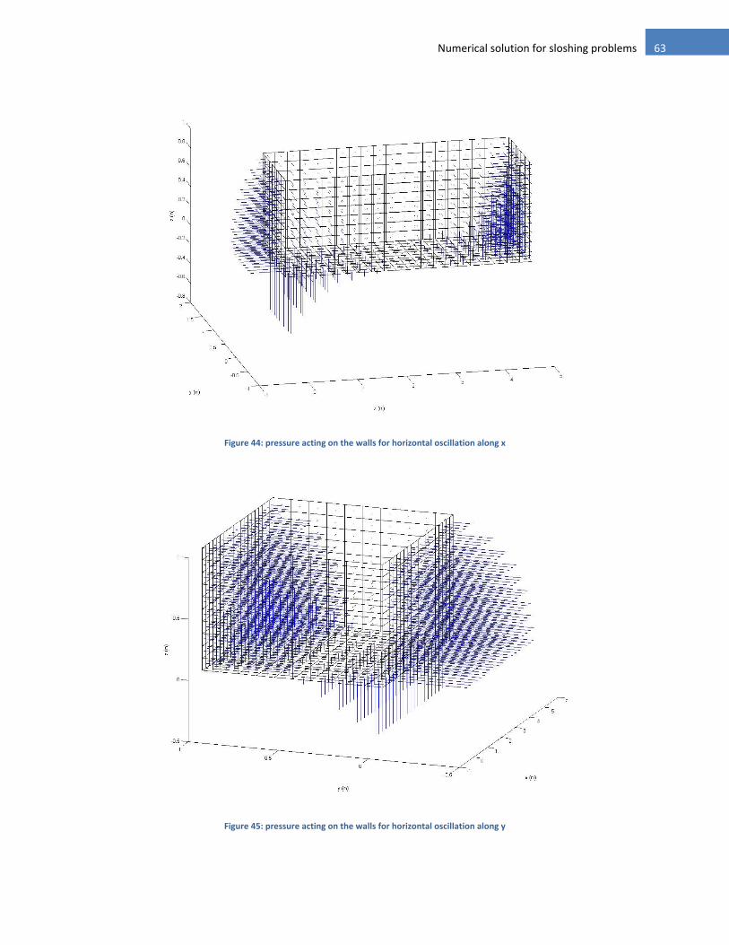
63 Numerical solution for sloshing problems
Figure 44: pressure acting on the walls for horizontal oscillation along x
Figure 45: pressure acting on the walls for horizontal oscillation along y

64 Fluid-structure interaction
Figure 46: pressure acting on the walls for vertical oscillation
And we can study resonant sloshing with the graph of the added mass as a function of frequency (Figure 47 and
Figure 48).
Figure 47: added mass as a function of frequency for oscillation along x

65 Numerical solution for sloshing problems
Figure 48: added mass as a function of frequency for oscillation along y
As a conclusion of this part, let’s say a few words about program performance. On the graphs depicted below, the
blue curve shows the ratio between the added mass provided by the program and the expected analytical
asymptotic added mass (Figure 49). The red curve represents the time needed by the program to compute the
value of the added mass.
Figure 49: slosh3D convergence test
0
1
2
3
4
5
6
7
8
9
10
0
0,1
0,2
0,3
0,4
0,5
0,6
0,7
0,8
0,9
1
0 96 192 288 384 480 576 672 768 864
Co
mp
uta
tio
n t
ime
(s)
Co
nve
rge
nce
Number of elements
Convergence test

66 Fluid-structure interaction
In this case, even a very low number of elements are sufficient to get decent results. It is particularly important to
adapt the meshing since the computation time increases quickly to several seconds long.
The difference of convergence between the 2D and 3D programs can be explained by the numerical integration of
Gauss’s functions, required to compute the influence coefficients. Indeed, in the program slosh2D, integral values
are estimated roughly by taking the mean value of the 2 nodes of the corresponding element. In the program
slosh3D, integral values are computed exactly thanks to the formula derived in Appendix 3.
4.4.2.2 EXTERNAL PROBLEM
By using Sommerfeld condition (the radiation condition that represents an infinite boundary) expressed in part
2.3.4, it is possible to analyze fluid-structure interaction for “external problems” (such as dam for example).
Actually, for high frequency oscillations, the Sommerfeld condition becomes . Thus, it is possible to model
fluid-structure interaction on a dam with a 3D rectangular “tank” with one vertical which is assigned the free
surface condition (in blue on the Figure 50 depicted below).
Figure 50: external problem geometry
One has to be careful with the distance between the structure and the imaginary boundary. It is recommended to
choose a distance of at least L = 5h, h being the height of the wet structure.
The program gives the pressure factor exerted on the dam. In the literature [15], hydrodynamics pressure factor on
a dam subjected to seismic action is given by Westergaard’s formula:
( )
√
On the graph depicted below, numerical results are compared with Westergaard’s formula that is widely used
(Figure 51). The height of the dam is taken equal to 1 m.
Values are almost identical in the upper part. However, a discrepancy appears when we get closer to the ground.
The shape of the numerical solution seems to be more accurate because we recognize the usual curve of pressure
distribution.
L
h

67 Numerical solution for sloshing problems
Figure 51: pressure factor on a dam - comparison of Westergaard's formula with numerical results
4.5 CONCLUSION
In this chapter, we have presented a way to solve numerically fluid-structure interaction. The resolution of Laplace
equation is done with an integral method. The Boundary Element Method is also used to obtain a linear system
which gives the velocity potential. Gauss functions are proposed to solve 2D and 3D problems.
The method is implemented in Matlab. The efficiency of the program has been studied by comparing the results
with the one found analytically in the previous chapter. Both programs are very effective. The only difficulty can be
the meshing of a 3D tank. It can require the use of other software.
0
0,1
0,2
0,3
0,4
0,5
0,6
0,7
0,8
0,9
1
0 0,2 0,4 0,6 0,8 1
z (m
)
Pressure factor (t/m)
Pressure factor exerted on a dam subjected to seismic action
Westergaard'sformula
Numericalsolution

68 Fluid-structure interaction
5 GENERAL CONCLUSION
In this study, different approaches are presented in order to analyze fluid-structure interaction which obeys a
Neumann problem. The equations have been derived in the first part, based on the assumption of a perfect fluid.
Two methods are presented: an analytical and a numerical solution.
We have presented 3 different ways to solve analytically the sloshing problem when a 2D rectangular tank, fixed to
the ground, is subjected to harmonic oscillations. Graham & Rodriguez and Hunt & Priestley’s methods are similar
in the approach of the problem: assumptions and equations are the same. The difference lies in the resolution of
the equation of sloshing. Graham & Rodriguez neglect the “transient state” of the response of the fluid. Thus, with
this model, it was like no waves were created due to the movement of the tank. The consequence is that the
pressure force is proportional to the ground acceleration with a coefficient called the added impulsive mass. The
impulsive mass represents the quantity of water that is moving in unison with the structure. Hunt & Priestley take
into account the “transient state”. The waves formed are oscillating in the tank without damping (so the transient
state is not really transient…), which leads to a convective force acting on the tank walls. This convective force is
the sum of n added convective mass (n being the number of sloshing modes) that are oscillating like a simple
oscillator having the frequency of the sloshing mode considered. The steady state gives the same impulsive force
than in Graham & Rodriguez’s method. Housner proposes an approximate method that gives simples formulas to
assess both of impulsive and convective forces. Actually, Housner takes into account only one sloshing mode for
the computation of the added convective mass. The results are very close to the ones found with Hunt & Priestley’s
method. We have also demonstrated that effects of resonant amplification of sloshing water are not relevant in the
case of seismic action.
Analytical solutions are really useful in order to understand phenomenon occurring in sloshing problems. They
provide good results and do not require any complicated theory: most of the time, the simple Housner formula is
sufficient to estimate the impulsive added mass. However, it only allows solving problems in a very limited number
of cases. Indeed, analytical solutions are only possible for simple geometry, namely rectangular and circular tanks.
Even if these 2 cases encompass a great majority of practical cases, it is possible to encounter more specific
geometry. That is why we propose a numerical solution that allows us to solve the problem for any kind of
geometry. The resolution of Laplace equation is done with an integral method. The Boundary Element Method is
also used to obtain a linear system which gives the velocity potential. Gauss functions are proposed to solve 2D and
3D problems. The program is implemented on MATLAB. The BEM is very efficient and provide accurate results.
The main point that still needs thorough investigation is fluid-structure coupling. All the work done in this study is
based on the assumption that structures have rigid walls. This is not always the case (in particular for steel tanks).
Structure deformations can influence on hydrodynamic pressure, and hydrodynamic pressure can then affect
structure deformations… It is thus necessary to couple the program proposed in this paper with structure software.
This coupling would require FEM-BEM coupling. In this case, resonant sloshing can become important.

69 General conclusion
REFERENCES [1] DAVIDOVICI, V. and HADDADI, A. – “Seismic calculation of tanks” (in French), Institut technique du bâtiment
et des travaux publics, 1982.
This document gives the results of the methods developed by Graham & Rodriguez, Hunt & Priestley and Housner.
It also proposes practical calculations. Despite several mistakes, it is a useful document that summarizes the
different known method at the time.
[2] EUROCODE 8 – “Design of structures for earthquake resistance – part 4: silos, tanks and pipelines”, European
Committee for Standardization, 1988.
The Eurocode 8.4 proposes an approach to compute the seismic response of tanks with graphs and abacus.
[3] DE LANGRE, E. – “Fluids and Solids” (in French), Les éditions de l’Ecole Polytechnique, 2006.
This book deals with the fluid-solid interactions and explains the phenomenon with equations. It also treats the
case of an oscillating tank filled with water.
[4] HUERRE, P. – “Fluid mechanics” (in French), Les éditions de l’Ecole Polytechnique, 1998.
This book presents assumptions and equations dealing with fluid mechanics problems.
[5] PECKER, A – “Structural dynamic of infrastructures” (in French), ENPC, 2007.
This document deals with the effects of seismic actions and gives tools to study the dynamic response of structures
(modal decomposition in particular).
[6] PESEUX, B. – “Introduction to fluid-structure coupling” (in French), Ecole Centrale Nantes, 2010.
This handout presents Green’s equations and the singularity method in order to solve fluid-structure problems.
[7] HEIN HOERNIG, R.O. – “Green’s functions and integral equations for the Laplace and Helmholtz operators in
impedance half-spaces”, Ecole Polytechnique, 2010.
This thesis presents the mathematical tools to compute Green’s function for Laplace equation. This is useful to
solve the problem with the singularity method.
[8] SEGHIR, A. – “Numerical modeling of seismic response of structures with ground-structure and fluid-structure
interaction” (in French), Université Paris-Est Marne-la-Valléé, 2011.
This thesis presents equations and numerical solutions for fluid-structure interaction problems. In particular, the
author gives boundary conditions in order to solve the external problem of radiation.
[9] US Army Corps of Engineers – “Time-History Dynamic Analysis of Concrete Hydraulic Structures”, Department
of the Army, 2003.
This manual describes procedures for the linear-elastic time-history dynamic analysis for seismic design and
evaluation of concrete hydraulic structures.

70 Fluid-structure interaction
[10] SCORLETTI, G. – “Signal processing” (in French), Ecole Centrale Lyon, 2011.
This handout deals with signal processing, in particular presents how to program the Fast Fourier Transform on
Matlab.
[11] Pacific Earthquake Engineering Research Center – “PEER Ground Motion Database”:
<http://peer.berkeley.edu/peer_ground_motion_database> (valid link February 20, 2013).
This website provides numerous data about earthquake, such as time-history recording.
[12] LEBON, J-D. – “Housner’s method for conical tanks in seismic area” (in French), Annales de l’institut
technique du bâtiment et des travaux publics N°491, February 1991.
This article shows how to use Hounser’s method for certain kind of tanks.
[13] GEORGAKIS, C.T., KOSS H.H. and DE TOFFOL W. – “Tuned Liquid Dampers for the New European Court of
Justice, Luxembourg”, Structural Engineering International, 4/2005.
Presentation and experimental verification of the performance of TLD put in place in the New European Court of
Justice.
[14] FUJII, K., TAMURA, Y., SATO, T. and WAKAHARA T. – “Wind-Induced vibration of tower and practical
applications of Tuned Sloshing Dampers”, Journal of Wind Engineering and Industrial Aerodynamics, 33 (1990)
263-272.
Presentation and experimental verification of the performance of TLD put in place in the Nagasaki Airport Tower
and Yokohama Marine Tower.
[15] http://www.physicsforums.com/showthread.php?t=129837 (valid link February 20, 2013).
Assumptions for the validity of the incompressible flow.
[16] Geodynamics and structures – “Dynamic risks for river marine structures. Fascicle n°4: Seismic action” (in
French), Centre d’études techniques maritimes et fluviales ER QG 94.05, August 1995.