fluids i menus
DESCRIPTION
manualTRANSCRIPT

FluidSIM® 5
User’s Guide
05/15

FluidSIM is a teaching tool for simulating pneumatics, hydraulics, electrics/electronics and digital technique. It can be used in combi-nation with the Festo Didactic GmbH & Co. KG training hardware, but also independently. FluidSIM was developed as a joint venture between the University of Paderborn, Festo Didactic GmbH & Co. KG, Denkendorf, and Art Systems Software GmbH, Paderborn.

© Festo Didactic GmbH & Co. KG • Art Systems GmbH • FluidSIM 3
Contents
1. Welcome! 14
2. Installation 17
2.1 Technical requirements 17 2.2 Installation with program activation 18 2.2.1 Important information about online activation 18 2.3 Installation with a license connector 19 2.4 Installing the full version from DVD-ROM 19
3. First steps 21
3.1 Create a new circuit drawing 21 3.2 Organize symbols, libraries and circuit diagrams 25 3.3 Insert symbol from menu 26 3.4 Symbol libraries 28 3.4.1 Create user library 29 3.5 Circuit files 30
4. Library and project window 31
4.1 Change window position 31 4.2 Automatic show and hide 31
5. Edit circuit 33
5.1 Insert and arrange symbols 33 5.2 Connect connectors / ports 33 5.3 Automatically connect connectors 35 5.4 Insert T distributor 37 5.5 Move lines 40 5.6 Direct connection via straight connection line 42 5.7 Define the characteristics of lines 43 5.8 Delete line 45

4 © Festo Didactic GmbH & Co. KG • Art Systems GmbH • FluidSIM
5.9 Set the properties of the connectors 45 5.10 Configure a way valve 47 5.11 Configure cylinders 49 5.12 Group symbols 51 5.13 Create macro objects 51 5.14 Delete symbol groups and macro objects 52 5.15 Align symbols 52 5.16 Mirror symbols 52 5.17 Rotate symbols 53 5.18 Scale symbols 54
6. Drawing frame 56
6.1 Editable labels 56 6.2 Use a drawing frame 57 6.3 Page dividers 61
7. Additional tools for creating drawings 65
7.1 Drawing tools 65 7.1.1 Grid 65 7.1.2 Alignment lines 65 7.1.3 Object snap 66 7.1.4 Rulers 67 7.2 Drawing levels 67 7.3 Cross-references 69 7.3.1 Create cross-references from symbols 71 7.3.2 Cross-reference representation 71 7.3.3 Manage cross-references 72 7.4 Drawing functions and graphical elements 74 7.4.1 Interruption/Potential 75 7.4.2 Conduction line 78 7.4.3 Line 80 7.4.4 Polyline (set of connected lines) 82 7.4.5 Rectangle 83 7.4.6 Circle 85 7.4.7 Ellipse 86

© Festo Didactic GmbH & Co. KG • Art Systems GmbH • FluidSIM 5
7.4.8 Text 88 7.4.9 Image 88 7.5 Check drawing 90
8. Simulating with FluidSIM 91
8.1 Simulation of existing circuits 91 8.2 The different simulation modes 93 8.2.1 Reset and restart of the simulation 94 8.2.2 Single step mode 94 8.2.3 Simulation to a state change 94 8.3 Simulating circuits you create yourself 95 8.3.1 Example with a pneumatic circuit 95 8.3.2 Example with a hydraulic circuit 103 8.3.3 Example with an electronic circuit 111
9. Advanced concepts in simulating and creating circuits 120
9.1 Adjusting the component parameters 120 9.2 Special settings for cylinders 124 9.2.1 Cylinder friction and cylinder mass 124 9.2.2 External load and friction 125 9.2.3 Force profile 128 9.2.4 Actuating labels 130 9.3 Special settings for directional control valves 131 9.3.1 Hydraulic resistance 131 9.4 Additional simulation functions 132 9.4.1 Simultaneous actuation of several components 133 9.4.2 Simulation of individual pages and entire projects 133 9.5 Displaying quantity values 134 9.5.1 Display of direction of quantity values in FluidSIM 136 9.6 Displaying state diagrams 137 9.7 Coupling hydraulics, pneumatics, electrics and mechanics
139 9.7.1 Display styles for labels 147 9.8 Operating switches 148 9.8.1 Switches at cylinders 149

6 © Festo Didactic GmbH & Co. KG • Art Systems GmbH • FluidSIM
9.8.2 Relays 151 9.8.3 Coupling mechanical switches 152 9.8.4 Automatic switch altering 152 9.9 Adjusting component parameters during the simulation 153 9.10 Settings for simulation 155 9.11 Use of the EasyPort-hardware 155 9.12 OPC and DDE communication with other applications 157 9.13 Open-loop and closed-loop control by using continuous
valves 159 9.13.1 Open-loop control in pneumatics 161 9.13.2 Open-loop control in hydraulics 163 9.13.3 Closed-loop control in pneumatics 166 9.13.4 Closed-loop control in hydraulics 172 9.14 Use of the oscilloscope in electronics 178 9.15 Simulation of rotating machines 180
10. GRAFCET 183
10.1 The various GRAFCET modes 183 10.1.1 Drawing only (GrafEdit) 184 10.1.2 Observation (GrafView) 184 10.1.3 Control (GrafControl) 184 10.2 Setting the GRAFCET mode 185 10.3 GRAFCET elements 185 10.3.1 Steps 186 10.3.2 Actions 188 10.3.3 Transitions 190 10.3.4 Stored effective actions (allocations) 193 10.3.5 GRAFCET-PLC component 194 10.4 Access to variables of circuit components 198 10.5 Monitoring with GRAFCET actions 201 10.6 Quick reference for the FluidSIM-relevant GRAFCET concepts
207 10.6.1 Initialization 207 10.6.2 Sequence rules 208 10.6.3 Sequence selection 208 10.6.4 Synchronization 208

© Festo Didactic GmbH & Co. KG • Art Systems GmbH • FluidSIM 7
10.6.5 Transient sequence / unstable step / virtual triggering 209 10.6.6 Determining the values of GRAFCET variables 209 10.6.7 Checking the entries 209 10.6.8 Admissible characters for steps and variables 210 10.6.9 Variable names 210 10.6.10 Functions and formula entry 211 10.6.11 Delays / time limits 212 10.6.12 Boolean value of an assertion 213 10.6.13 Target information 214 10.6.14 Partial GRAFCETs 214 10.6.15 Macro-steps 214 10.6.16 Compulsory commands 215 10.6.17 Enclosing step 215 10.6.18 Action when a transition is triggered 216
11. Dimension 217
11.1 Draw dimension 217 11.2 Settings for the dimension 218
12. Component attributes 220
12.1 Component attributes in the Properties dialog window 221 12.2 User Defined Properties 223 12.3 Drawing Properties 224 12.4 Main and secondary components 225 12.5 Linking main and secondary components 225 12.6 Link solenoid valves and solenoid coils 227 12.7 Attributes of the text components 231 12.8 Link text components with attributes 234 12.9 Text components with specified links 236 12.10 Change the properties of multiple objects simultaneously
237 12.10.1 Drawing Properties 237 12.10.2 Main Component 239

8 © Festo Didactic GmbH & Co. KG • Art Systems GmbH • FluidSIM
13. Parts list management and analyses 241
13.1 Display parts list 242 13.2 Find components from the parts on the circuit diagram 243 13.3 Set parts list properties 245 13.4 Export parts list 248 13.5 Insert tube list 249
14. Manage projects 252
14.1 Create new project 252 14.2 Project nodes 253 14.2.1 Project archiving 253 14.3 Circuit and parts list nodes 254
15. Circuit and project properties 256
15.1 Attributes 257 15.1.1 Predefined placeholders 259 15.2 Page Dividers 260 15.3 Basic Unit Length 260 15.4 Encryption 261 15.5 Cross Reference Representation 263
16. Special functions for electric circuits 264
16.1 Potentials and conduction lines 264 16.2 Cables and wiring 266 16.2.1 Manage cables 272 16.2.2 Insert cable map 273 16.2.3 Insert cable list 275 16.2.4 Insert wiring list 278 16.3 Terminals and terminal strips 281 16.3.1 Set terminals 281 16.3.2 Set multiple terminals 283 16.3.3 Create terminal strips 285 16.3.4 Manage terminal strips 286

© Festo Didactic GmbH & Co. KG • Art Systems GmbH • FluidSIM 9
16.4 Terminal diagram 288 16.4.1 Set links 290 16.5 Contact images 294
17. Circuit input and output 297
17.1 Print circuit diagram and parts list 297 17.2 Import DXF file 299 17.3 Export circuit 299
18. Options 301
18.1 General 301 18.2 Save 302 18.3 Folder Locations 303 18.4 Language 304 18.5 Dimension 304 18.6 Cross Reference Representation 306 18.7 Connector Links 307 18.8 Warnings 308 18.9 Automatic Updates 309 18.10 Simulation 310 18.11 GRAFCET 312 18.12 DDE Connection 313 18.13 Environment parameters 313 18.14 Fluid properties 314 18.15 Sound 314 18.16 Text Sizes 316
19. Menu overview 317
19.1 File 317 19.2 Edit 320 19.3 Insert 322 19.4 Draw 324 19.5 Page 325 19.6 Execute 326

10 © Festo Didactic GmbH & Co. KG • Art Systems GmbH • FluidSIM
19.7 Didactics 327 19.8 Project 328 19.9 View 329 19.10 Library 333 19.11 Tools 334 19.12 Window 335 19.13 Help 336
20. Functional diagram 337
20.1 Edit Mode 338 20.1.1 Set diagram properties 338 20.1.2 Table textboxes 339 20.1.3 Adjust the presentation of the diagrams 342 20.2 Draw diagram curve 343 20.3 Insert signal elements 344 20.4 Insert text boxes 345 20.5 Draw signal lines and insert signal connections 347 20.5.1 Free-draw signal lines 347 20.5.2 Drawing signal lines from signals 349 20.5.3 Draw signal lines from diagram support points 349 20.6 Insert additional signal lines 350 20.7 Insert row 350 20.8 Delete row 350 20.9 Additional editing functions 351 20.9.1 Zoom 351 20.9.2 Undo editing steps 351
21. The Component Library 352
21.1 Hydraulic Components 352 21.1.1 Service Components 352 21.1.2 Configurable Way Valves 360 21.1.3 Mechanically Actuated Directional Valves 364 21.1.4 Solenoid-actuated Directional Valves 372 21.1.5 Shutoff Valves 378 21.1.6 Pressure Control Valves 381

© Festo Didactic GmbH & Co. KG • Art Systems GmbH • FluidSIM 11
21.1.7 Pressure Switches 393 21.1.8 Flow Control Valves 393 21.1.9 Continuous valves 397 21.1.10 Actuators 402 21.1.11 Measuring Devices 408 21.2 Pneumatic Components 410 21.2.1 Supply Elements 410 21.2.2 Configurable Way Valves 417 21.2.3 Mechanically Operated Directional Valves 421 21.2.4 Solenoid Operated Directional Valves 429 21.2.5 Pneumatically Operated Directional Valves 433 21.2.6 Shutoff Valves and Flow Control Valves 437 21.2.7 Pressure Operated Switches 443 21.2.8 Pressure Operated Switches 447 21.2.9 Vacuum Technique 448 21.2.10 Valve Groups 451 21.2.11 Continuous valves 454 21.2.12 Actuators 454 21.2.13 Measuring Instruments 463 21.3 Electrical Components 468 21.3.1 Power Supply 468 21.3.2 Actuators / Signal Devices 471 21.3.3 Measuring Instruments / Sensors 473 21.3.4 General Switches 476 21.3.5 Delay Switches 477 21.3.6 Limit Switches 479 21.3.7 Manually Operated Switches 481 21.3.8 Pressure Switches 482 21.3.9 Proximity Switches 484 21.3.10 Relay 485 21.3.11 Controller 487 21.3.12 EasyPort/OPC/DDE Components 489 21.4 Electrical Components (American Standard) 491 21.4.1 Power Supply 491 21.4.2 General Switches 491 21.4.3 Delay Switches 492 21.4.4 Limit Switches 493

12 © Festo Didactic GmbH & Co. KG • Art Systems GmbH • FluidSIM
21.4.5 Manually Operated Switches 494 21.4.6 Pressure Switches 495 21.4.7 Relays 496 21.5 Electronic components 497 21.5.1 Power supply 497 21.5.2 Passive components 500 21.5.3 Semiconductor 504 21.5.4 Measuring instruments / Sensors 511 21.5.5 Switches 513 21.5.6 Machines 516 21.5.7 Controller 533 21.5.8 Controller (block diagram) 542 21.6 Digital Components 546 21.6.1 Constants and Terminals 546 21.6.2 Basic Functions 548 21.6.3 Special Functions 550 21.7 GRAFCET Elements 556 21.7.1 GRAFCET 556 21.8 Miscellaneous 559 21.8.1 Miscellaneous 559
22. Learning, Teaching, and Visualizing Technologies 564
22.1 Information about Single Components 564 22.1.1 Component Descriptions 565 22.1.2 Component Illustrations 567 22.2 Selecting Didactics Material from a List 573 22.2.1 Tutorial 573 22.2.2 Component Library 575 22.2.3 Didactics Material 577 22.3 Presentations: Combining Instructional Material 579 22.4 Extended Presentations in the Microsoft PowerPoint Format
585
23. Didactics Material Survey (Pneumatics) 588
23.1 Basics 588

© Festo Didactic GmbH & Co. KG • Art Systems GmbH • FluidSIM 13
23.2 Supply elements 590 23.3 Actuators 595 23.4 Directional control valves 600 23.5 Shutoff valves 611 23.6 Flow control valves 618 23.7 Pressure control valves 620 23.8 Time delay valve 622 23.9 Sequential circuit and signal overlap circuit 625 23.10 Educational Films 627 23.10.1 Educational Films 627 23.11 Standard Presentations 628 23.11.1 Presentations 628
24. Didactics Material Survey (Hydraulics) 630
24.1 Applications 630 24.2 Components of a Hydraulic Plant 631 24.3 Symbols 633 24.4 Some Physical Fundamentals 637 24.5 Components of a Power Unit 640 24.6 Fundamentals of Valves 644 24.7 Pressure Valves 646 24.8 Way Valves 653 24.9 Shutoff Valves 662 24.10 Flow Valves 666 24.11 Hydraulic Cylinders and Motors 669 24.12 Gauges 672 24.13 Exercises 673 24.14 Educational Films 683 24.14.1 Educational Films 683 24.15 Standard Presentations 683 24.15.1 Presentations 684
Index 685

Welcome!
14 © Festo Didactic GmbH & Co. KG • Art Systems GmbH • FluidSIM
Chapter 11. Welcome!
Welcome to FluidSIM!
Thank you for purchasing the FluidSIM training software. This user’s guide functions both as an introduction to FluidSIM and as a reference manual outlining the possibilities, concepts and opera-tion of the software package. This guide is not designed for the teaching of training content in fluid engineering or electronics; if you require materials for that purpose, there are textbooks availa-ble from Festo Didactic GmbH & Co. KG.
FluidSIM permits the creation and simulation of circuits in the following fields:
— Electro-pneumatics/vacuum technology
— Electro-hydraulics/mobile hydraulics
— Electrical engineering/electronics
There are specialized versions of the program for each of these technologies, referred to in the following as FluidSIM-P, FluidSIM-H and FluidSIM-E respectively.
All three versions also contain components for drawing creation and simulation of:
— Digital technology
— GRAFCET
Some of the functions and components described in this manual may not be available, depending on which program versions you purchased. In places where the programming differences between the technologies are only minor, general examples are given, and the specific differences are mentioned. When specialized functions are explained, such as closed-loop control in pneumatics and in hydraulics, a separate chapter is devoted to each function.
For the first time you can link all technologies in FluidSIM in a single circuit or project. This means that if you have purchased all three technology versions, you can utilize pneumatic, hydraulics, control technology, electronics, digital technology etc. in any way you want

© Festo Didactic GmbH & Co. KG • Art Systems GmbH • FluidSIM 15
in a single technical system. FluidSIM ensures that you can only join connections which are also physically possible.
A major feature of FluidSIM is its close linkage between CAD func-tionality and simulation. On the one hand, FluidSIM allows DIN-compliant drawing of fluidic and electronic circuit diagrams; on the other hand, it is capable of using physical component descriptions to carry out a realistic, dynamic simulation of the drawn circuit. This practically eliminates the separation between drawing creation and simulation.
When developing FluidSIM, special emphasis was placed on mak-ing operation intuitive and easy to learn. This approach makes it possible for you to learn to design and simulate fluidic and elec-tronic circuit diagrams in a very short time. To provide access to professional functions not present in this simple operating inter-face, FluidSIM also has an “Expert Mode” which can be switched on as needed.
FluidSIM-P was created by the “Knowledge-based Systems” workgroup at the University of Paderborn. FluidSIM-H is the result of cooperative research between the Instrumentation and Control department at Gerhard Mercator University in Duisburg, and Knowledge-based Systems at the University of Paderborn. On hand for mechanical engineering matters was Dr Ralf Lemmen. FluidSIM-E was developed as an entirely new module by Art Systems Soft-ware GmbH.
Planning and development of FluidSIM: Dr Daniel Curatolo, Dr Marcus Hoffmann and Dr Benno Stein.
Users of this software are encouraged to contribute tips, criticism, and suggestions for improvement of FluidSIM via email.
You can also find the newest version on the following websites:
www.fluidsim.de
www.festo-didactic.de

16 © Festo Didactic GmbH & Co. KG • Art Systems GmbH • FluidSIM
Installation
© Festo Didactic GmbH & Co. KG • Art Systems GmbH • FluidSIM 17
Chapter 22. Installation
With your purchase of the full version of FluidSIM, you received one or more DVD-ROMs and possibly a license connector. The installa-tion procedure is described in the following sections.
The full version of FluidSIM is available in two versions: a version that supports automatic Online activation, and the version with a license connector for insertion in a USB port.
2.1 Technical requirements
You need a computer running Windows XP (SP3), Windows Vista, Windows 7 or Windows 8.
If you intend to simulate complex circuits, a computer with dual processor is recommended. Stand-alone tablet PCs without a physically connected mouse are not ideal because creating draw-ings is impractical using only swipe and gesture control.
During simulation, most of the adjustable components can be controlled using a game controller as an alternative to the mouse. You can use any game controller which Windows recognizes and which appears in the Control Panel. You may need the matching device drivers for Windows.
Additional drivers may be necessary in order to link FluidSIM to external hardware. Compatible drivers for Festo’s EasyPort can be found in the Support subfolder on the DVD. Communication with other applications via OPC requires special auxiliary modules, which are likewise located in the Support folder. For more details
about OPC, see the section OPC and DDE communication with other applications.

18 © Festo Didactic GmbH & Co. KG • Art Systems GmbH • FluidSIM
2.2 Installation with program activation
We recommend activating the program via a PC connected to the internet. During installation, you will be prompted to activate FluidSIM. There are three ways of doing so:
— Online activation This variant allows fully automatic activation if the installation PC has direct access to the internet.
— Indirect activation In this case the PC on which FluidSIM is to be installed does not need to have direct internet access. Instead, the subsequent dialog window gives you an internet address and an individual-ly generated license key. You can then generate a matching ac-tivation code by accessing the displayed internet address from any computer. You then enter that activation code in the field provided in the activation dialog box on the installation PC.
— Call Festo to receive your activation code If you do not have an internet connection or if the internet con-nection fails, you can call our service staff on weekdays during standard office hours and they will provide you with your acti-vation code.
2.2.1 Important information about online activation
During program activation, the individual features of your PC’s hardware are linked to the product ID and used to generate an activation code which is valid only for that PC. If at some later time you intend to modify your PC substantially or want to use a new PC, you can transfer the license. To do so, you first have to deactivate the license on the original PC, by uninstalling the program. You can find the deinstallation procedure in the Control Panel in “Add or Remove Programs” or “Programs”.

© Festo Didactic GmbH & Co. KG • Art Systems GmbH • FluidSIM 19
If the PC on which you installed FluidSIM is no longer functional or deactivation fails for some other reason, as an exception you can transfer the license without prior deactivation.
Please note that this type of license transfer (without prior deacti-vation) is only possible a few times. Moreover, when you transfer a license to a modified or new PC, activation is no longer possible on the original PC. Once the license is transferred, you cannot activate FluidSIM on the original PC without a prior deactivation.
2.3 Installation with a license connector
Depending on whether you purchased a multiple or single user license, this special connector is either connected directly to the local user’s computer or is on a license server at a central location in your network.
In the case of network licensing, the connector defines how many instances of FluidSIM can run simultaneously on the network. If you try to start more instances of FluidSIM than are permitted, you will see a corresponding error message. If the license server is down or the license connector is no longer present, you will be able to save any circuits you are working on before FluidSIM terminates. As soon as the license server becomes available again, you can re-sume your work.
Detailed information on network installation of FluidSIM can be found in the installation guide included as a booklet in the product packaging, and also in electronic form as a PDF file in the “Doc” folder on the installation DVD.
2.4 Installing the full version from DVD-ROM
If you are using the software with a license connector, do not plug it in until you are prompted to do so by the installation program.

20 © Festo Didactic GmbH & Co. KG • Art Systems GmbH • FluidSIM
→ Switch on your computer and log on with administrator rights.
→ Insert the DVD-ROM.
Usually the installation program starts automatically. If it doesn’t, please start it manually.
After a few seconds the start screen of the installation program appears. Here you can select whether you have received the ver-sion for online activation or a license connector with the FluidSIM package.
Note that there are two versions of the license connector: The newer one is silver in color and has the product label “CodeMeter”. If you have purchased FluidSIM as an update of an earlier version, you can also continue to use your existing green “WibuKey” con-nector if it has been reprogrammed accordingly.
For online activation, you do not need a license connector; instead you require your individual product ID which is printed on the back of the DVD case.
→ Follow the instructions of the installation program. If you are not sure how to answer any of the questions, simply click
Next .

First steps
© Festo Didactic GmbH & Co. KG • Art Systems GmbH • FluidSIM 21
Chapter 33. First steps
3.1 Create a new circuit drawing
When you start FluidSIM, the system checks whether you have installed more than one technology (pneumatics, hydraulics, elec-tronics). If you have, the selection window appears listing the available technologies. Here you specify which components and program functions you wish to use in this program session. This decision is especially important for network users because a li-cense will be occupied for each technology until you exit FluidSIM. You can restart FluidSIM at any time and select a different combina-tion.
Figure 3/1: Select Technologies dialog window
The available technologies and the currently free licenses are displayed here.
FluidSIM remembers the last selection and suggests it when the program is next started. If you frequently use different combina-tions, you can create links which will allow you to start FluidSIM directly with the corresponding selection.
Next, the key concepts and terms are described which you will encounter when using FluidSIM.
Available technologies

22 © Festo Didactic GmbH & Co. KG • Art Systems GmbH • FluidSIM
→ Start FluidSIM with the selection you require.
→ In the menu File , select New / File... .
An empty circuit window opens in which you can insert symbols and connect them with lines. First you should set the drawing size.
→ In the Page menu, select Paper Size... .

© Festo Didactic GmbH & Co. KG • Art Systems GmbH • FluidSIM 23
Figure 3/2: Page dialog window, Drawing Size tab: setting the
drawing size
If you use a drawing frame, then FluidSIM can automatically adjust the paper size. If you wish to define the drawing size manually, then deactivate the “Adopt from drawing frame” option and select the dimensions and orientation you require for the drawing. If the drawing’s dimensions are larger than your printer’s printing area then you can distribute your drawing across several pages (tile).
To retain a better overview you can create attributes for every circuit drawing.

24 © Festo Didactic GmbH & Co. KG • Art Systems GmbH • FluidSIM
→ Click the “Attributes” tab.
Figure 3/3: Page dialog window, Attributes tab: creating attrib-
utes
The attribute table allows you to save any desired data in the form of attribute value pairs. The associated placeholders (attributes with the same name) in the drawing frame are replaced by the values entered.

© Festo Didactic GmbH & Co. KG • Art Systems GmbH • FluidSIM 25
You can also access this dialog window directly by using the Page
menu and the Properties... menu item.
3.2 Organize symbols, libraries and circuit diagrams
In order to support the organization of the different document types in FluidSIM all of the circuit files are assigned to one of three groups.
Symbols are formal, abstract models providing a graphical repre-sentation of the function of a component or component group. This can consist of simple circuit symbols or entire circuits. Symbols can be inserted into their own circuits and linked between the connect-
ing points. The insert can be performed either via the Insert menu
or via drag and drop from a library window. Symbols can be com-piled into library files with the lib file suffix.
Libraries are hierarchically organized collections of symbols. In addition to the standard library, which users cannot modify, users can compile any desired number of their own libraries. You can find
functions for organizing the libraries on the Library menu as well
as on the context menu of the currently active library. To switch libraries use the tab in the upper margin of the library window. Library files have the lib file suffix.
The default location for circuits is in the FluidSIM folder con-
tained in the My Documents folder defined by the operating sys-tem. These have the circ file suffix.
Note: It is worthwhile to create a new sub-folder in the FluidSIM
directory for every customer or every project.
Symbols
Libraries
Circuits

26 © Festo Didactic GmbH & Co. KG • Art Systems GmbH • FluidSIM
3.3 Insert symbol from menu
To find a specific symbol you can either enter characteristic key words in the Find Symbol dialog windows or navigate through the hierarchical structure.
→ Where necessary open a new window and select the Find
Symbol Description... entry on the Insert menu.
The Find Symbol dialog window then opens. You can enter your search terms in the “Search” input line. Separate the individual search terms using commas or spaces. Neither the order of the search terms nor upper or lower case letters have any influence on the search results.

© Festo Didactic GmbH & Co. KG • Art Systems GmbH • FluidSIM 27
Figure 3/4: Find Symbol dialog window
You can see the symbols found in the two results lists. The library hierarchy is displayed on the left-hand side although only those branches appear which contain matching symbols. An alphabetical list of the search hits is displayed on the right-hand side. The sym-bol of the highlighted entry is shown in the preview. Once you have found the symbol that you were looking for, you can select it using
the &OK button or by double-clicking on the appropriate row in
the results list. The symbol then “hangs” on the mouse pointer and is placed by left-clicking on the drawing area.

28 © Festo Didactic GmbH & Co. KG • Art Systems GmbH • FluidSIM
With the Fuzzy Search option you can activate a tolerance in order to achieve results despite minor typing errors or spelling variants.
3.4 Symbol libraries
FluidSIM is capable of managing multiple libraries, each of which is displayed in a tab in the library window. Libraries which cannot be modified in FluidSIM are labeled with a lock symbol in the tab. This applies to standard library as well as to symbol folders which FluidSIM does not manage itself or for which the registered user does on possess write authorization.
Every library is displayed hierarchically. Every hierarchy level can by shown or hidden by clicking on the group name. Right-clicking in a library opens a context menu offering the following menu items for editing the library:
Defines the size of the symbols displayed. Small , Normal and
Large are available.
Opens all of the hierarchy levels.
Closes all of the hierarchy levels.
There are three types of library:
This library is delivered with FluidSIM and cannot be modified.
Circuit and symbol files saved on the disk can be used as libraries in FluidSIM. The files from the selected folder are added as a library
via the Library menu and the Add Existing Symbol Folder...
menu item. The library hierarchy corresponds exactly to the folder hierarchy. These libraries cannot be modified in FluidSIM. The files must be modified directly.
You can create and subsequently edit new libraries via the Library
menu and the Add New Library... menu item (see section Create
View
Expand All
Collapse All
The standard library
Symbol folders
User libraries

© Festo Didactic GmbH & Co. KG • Art Systems GmbH • FluidSIM 29
user library). Using drag and drop you can move the symbols and groups within the library as desired.
3.4.1 Create user library
In order to be able to access frequently used symbols (or circuits) more quickly multiple symbols can be compiled into libraries. Libraries are saved as files with the lib file suffix. You can create
new libraries using the Library and the Add New Library... menu
item. Right-clicking in the new library opens a context menu with which you can modify the library.
The following options are available:
Copies the selected symbols to the clipboard
Inserts the symbols into the library from the clipboard. These symbols can also be partial circuits.
Removes the selected symbols from the library.
Edits the text which libraries display below the symbol.
Opens a dialog window for selecting symbol files to be copied into the library as new symbols.
Copies the selected symbols into another library. The available libraries are listed in a submenu. Only the currently open libraries are displayed here (appearing as tabs in the library window) which are not write-protects (recognizable as no lock symbol is dis-played).
Creates a new hierarchy level below the active group. The active group is the one belonging to the area below the mouse point and can be recognized by the dark blue coloring.
Removes the hierarchy level which the mouse pointer is located in.
Copy
Paste
Delete
Rename...
Add Existing Symbols...
Copy to Other Library
New Sub-Folder...
Remove Sub-Folder

30 © Festo Didactic GmbH & Co. KG • Art Systems GmbH • FluidSIM
Enables you to rename the hierarchy level which the mouse pointer is located in.
3.5 Circuit files
FluidSIM circuit files have the circ file suffix and are saved as
compressed XML files. An option in the Save tab under the Op-
tions... menu item from the Tools menu allows you to deactivate
this compression so that the circuit files can be viewed as plain text. This can be useful for version management software, for example.
However, please note that editing a circ file outside FluidSIM can
cause the file to become unreadable or corrupted upon re-import.
Rename Sub-Folder...

Library and project window
© Festo Didactic GmbH & Co. KG • Art Systems GmbH • FluidSIM 31
Chapter 44. Library and project window
4.1 Change window position
The library window is anchored on the left-hand side by default and the project window (when a project is open) is on the right-hand side.
To separate the window from the anchor move the mouse pointer to the upper margin. Click and hold the left mouse button. Move the window a small distance towards the center of the screen. Now release the left mouse button. Now you need to move the library window to the lower right and the project window to the lower left. Once a window has been separated from the anchor it can be moved freely.
To re-anchor the window move the mouse pointer to the upper margin. Click and hold the left mouse button. Move the window as far as possible to the right or the left. Now release the left mouse button. This window snaps into place. This enables you to anchor the library window to the right and the project window to the left, for example. You can also anchor both windows on the same side. In this case you can move the desired window into the foreground by clicking the associated tab.
4.2 Automatic show and hide
The tabs offer an additional, practical function: Automatically showing and hiding the library or project window. Click the associ-ated vertical tab “Library” or “Project” at the edge of the window. This causes the window to be hidden providing a larger area for the drawing. In order to make the window visible again move the mouse pointer over the tab; the window opens once again. As soon as you have performed your operations in this window and move the mouse pointer to a circuit window the library window and / or

32 © Festo Didactic GmbH & Co. KG • Art Systems GmbH • FluidSIM
the project window are automatically hidden. To deactivate the function click the associated tab again (this then appears de-pressed).

Edit circuit
© Festo Didactic GmbH & Co. KG • Art Systems GmbH • FluidSIM 33
Chapter 55. Edit circuit
5.1 Insert and arrange symbols
You can insert symbols into the symbol window being edited using the dialog window Find Symbol and by means of the libraries. You can also transfer objects from every other window by selecting them and dragging them to the desired window. Alternatively you can also utilize the clipboard by selecting the items, choosing the
Copy menu item on the Edit menu, bringing the target window
into the foreground and selecting the Paste menu item on the
Edit menu. Using the mouse pointer to drag objects from one
window to another copies them. Dragging the objects from one position to another within a window moves them. In order to copy
within a window you need to hold down the Shift key while
moving the mouse pointer. You can recognize operation by the shape of the mouse pointer. During a move-operation a cross with arrows appears, when copying a plus symbol also appears in the lower right-hand corner of the cross.
5.2 Connect connectors / ports
In order to connect two component connectors with a line move the mouse pointer to the component connector. You can recognize a connector by the small circle at the end of a symbol’s connection line. As soon as you have touched the line the mouse pointer trans-forms into a crosshair .

34 © Festo Didactic GmbH & Co. KG • Art Systems GmbH • FluidSIM
Figure 5/1: Mouse pointer as a crosshair over a component con-nector.
→ Now press the left mouse button and move the mouse pointer to the connector which you wish to connect with the first.
You can recognize when you are over the connector by the shape of the mouse pointer . If the mouse pointer is over a connector which is already connected to a line then the prohibited sign appears and no line can be connected.
→ Release the mouse button once you have touched the second connector.
FluidSIM automatically lays a line between the two connectors.

© Festo Didactic GmbH & Co. KG • Art Systems GmbH • FluidSIM 35
Figure 5/2: Line between two connectors
Support points can be set when dragging lines. To do so simply release the mouse button while dragging the line and click the desired points. The line is completed as soon as you click a second connector or the same point twice. You can cancel the action by
pressing the Esc key or the right mouse button.
5.3 Automatically connect connectors
FluidSIM supports two methods of automatically connecting con-nectors. The first is to drop a symbol on an existing line. To be able to use this method, the symbol must have at least two connectors that precisely fit onto one or more existing lines and the lines that

36 © Festo Didactic GmbH & Co. KG • Art Systems GmbH • FluidSIM
will be produced must not cross the symbol. The following two illustrations show this function.
Figure 5/3: Circuit before the connectors are automatically con-nected
Figure 5/4: Circuit after the connectors are automatically connected
Another method of automatically connecting connectors is to position symbols so that their connectors can be horizontally or vertically connected with free connectors from other symbols. After the symbol has been dropped the corresponding lines are automat-ically drawn if they do not cross any symbols. The free connectors can also be T distributors.
You can define how different objects' connectors are automatically
connected in the Connector Links tab under the Options... menu

© Festo Didactic GmbH & Co. KG • Art Systems GmbH • FluidSIM 37
item from the Tools menu. The following two illustrations show
this function.
Figure 5/5: Circuit before the connectors are automatically con-nected
Figure 5/6: Circuit after the connectors are automatically connected
5.4 Insert T distributor
You do not need to utilize a special symbol in order to insert a T distributor. FluidSIM automatically inserts a T distributor when you lay a component connection on a line or lay a line segment to a connection. If you wish to connect two lines then you can also draw one line segment to another; FluidSIM then inserts two T distribu-tors and connects these with a new line.
→ Move the mouse points to a connector and press the left mouse button.

38 © Festo Didactic GmbH & Co. KG • Art Systems GmbH • FluidSIM
As soon as you touch the line the mouse pointer transforms into a crosshair .
→ Release the mouse button once you have touched the desired point on the line.
FluidSIM inserts a T distributor and automatically lays a line.
Figure 5/7: Line connection with inserted T distributor
Every T distributor can connect up to 4 lines with each other.
The default representation for the T distributor can be selected via the corresponding drop-down list on the toolbar.
You can customize the representation of the T distributor by dou-ble-clicking the T distributor or highlighting the T distributor and
selecting the Properties... menu item from the Edit menu. The

© Festo Didactic GmbH & Co. KG • Art Systems GmbH • FluidSIM 39
“Properties” dialog window opens. Select the “Representation” tab.
Figure 5/8: T distributor dialog window. Tab: Representation
Defines the representation of the basic T distributor. Here you can select whether the distributor should be represented as a filled circle or a simple intersection.
Defines that the T distributor should be represented as an electric link. This representation has a knock-on effect on the connected lines, which are automatically marked as links.
T distributor
Cross-Link

40 © Festo Didactic GmbH & Co. KG • Art Systems GmbH • FluidSIM
Defines that the T distributor should be represented as an electric junction. This representation has a knock-on effect on the termi-nals' target search. With a junction, the target in the direction of a straight line or right angle is found first and then the target via an angled branch.
5.5 Move lines
Once you have joined two connectors you can then adjust the length of the lines. You can move the line segments in parallel by moving the respective line segment. You can see when you have touched the line on the basis of the line-selection shape of the mouse pointer.
→ Press the left mouse button and move the line segment or-thogonally to the desired position.
Figure 5/9: Moving a line segment
→ Release the left mouse button; FluidSIM adjusts the adjoining line segments in such a way that they remain connected.
If you move a line segment with is directly connected to a compo-nent connector then FluidSIM may insert additional line segments in order to prevent gaps.
Junction

© Festo Didactic GmbH & Co. KG • Art Systems GmbH • FluidSIM 41
If you move a line segment that is horizontally or vertically con-nected with other line segments via T distributors then these line segments are moved together with the T distributors.
Figure 5/10: Moving multiple line segments
Figure 5/11: Moving multiple line segments
If you only want to move the individual line segment in the case described above then release the mouse button after you highlight the line segment. Click the segment again and move it while keep-ing the mouse button pressed.

42 © Festo Didactic GmbH & Co. KG • Art Systems GmbH • FluidSIM
Figure 5/12: Moving an individual line segment
5.6 Direct connection via straight connection line
Normally connection lines in technical circuits are always drawn orthogonally. However, it can sometimes be desirable to create a direct connection between two connectors via a diagonal line. To achieve this, first connect the two connectors in the standard way. Then select any segment on the line and right-click to open the context menu. Select “Straight connection line” to create a direct connection.
Figure 5/13: Direct connections between two connectors
To switch back to an orthogonal line, open the context menu again and select “Orthogonal line segments”.

© Festo Didactic GmbH & Co. KG • Art Systems GmbH • FluidSIM 43
5.7 Define the characteristics of lines
Lines, like other symbols, can be assigned an identification, cata-logue properties and user-defined properties. You can find further information on this under Component attributes in the Properties dialog window.
You can also define the style, color and drawing layer of the lines by double-clicking a line segment or highlighting the line segment and
selecting the Properties... menu item from the Edit menu. The
Line Properties dialog window opens. Select the Drawing Properties tab in this window. The settings are applied to the entire line sec-tion as far as the next connector or T distributor.

44 © Festo Didactic GmbH & Co. KG • Art Systems GmbH • FluidSIM
Figure 5/14: Line Properties dialog window: defining the properties of a pneumatic or electric line
Sets the drawing layer of the line.
Sets the color of the line.
Sets the line style of the line.
Sets the line thickness of the line.
Note: Working lines are typically displayed as solid lines, pilot lines as dashed lines.
Please note that the way the lines are displayed during the simula-tion depends on the physical status of the lines. The colors, line styles, and line thicknesses will vary according to pressure, flow,
Layer
Color
Line Style
Line Width

© Festo Didactic GmbH & Co. KG • Art Systems GmbH • FluidSIM 45
voltage, etc.. You can define how the lines are displayed during the
simulation on the Simulation tab under Options... in the Tools
menu. When you exit Simulation Mode, the lines once again appear the way you defined them in Edit Mode.
5.8 Delete line
To delete a line you can either highlight an associated line segment
and press the Del key or select the Delete menu item from the
Edit menu or highlight a component connector and press the
Del key. In these cases it is the line rather than the connector
itself that is deleted.
If you delete a T distributor which three or four lines are attached to then all of the lines are deleted. If, on the other hand, only two lines are connected then only the T distributor is deleted and the two lines combined into one.
5.9 Set the properties of the connectors
You can assign a component connector an identification and a blanking plug or silencer by double-clicking on the connector or by
selecting the connector and choosing the Properties... menu item
on the Edit menu. The Connector dialog window then opens.

46 © Festo Didactic GmbH & Co. KG • Art Systems GmbH • FluidSIM
Figure 5/15: Connector dialog window: setting the properties of a connector
You can enter a text identifying this connector into the input line. If the Display option is activated then the identification is displayed in the circuit diagram.
Whether or not the identification is actually displayed depends on
the option selected under Show Connector Descriptions .
During the simulation, the calculated quantity values can be dis-played not only with specialized measuring devices, but also direct-
ly at the connectors. For a quick overview, you can use View
Quantity Values... to show all values at all connectors with a
single click. As this is generally fairly confusing, you can also choose to view the quantity values at selected connectors only. For more details, see "Displaying quantity values".
Open the symbol list containing connector terminators by clicking the button using the arrow. Select a suitable silencer or a blanking plug.
Note: Please note that this symbol list is only available if a line is not connected to the connector in question. If you wish to connect a
Identification
Display quantity values
Terminator

© Festo Didactic GmbH & Co. KG • Art Systems GmbH • FluidSIM 47
line to a sealed connector you first have to remove the blanking plug or silencer. To do this select the empty field in the symbol list with the connector terminators. The alignment of the connector terminator can be set via the radio buttons.
5.10 Configure a way valve
If you require a certain valve which you cannot find in the standard FluidSIM library you can create your own valve symbol with the help of the valve editor.
→ Insert a 5/n-way valve into a circuit window from the “Stand-ard Symbols / Pneumatic Symbols / Valves / Configurable Way Valves” library (insert a hydraulic valve in case of FluidSIM-H).
To set the valve body and the actuation types of the way valves double-click the valve. The dialog window Properties then opens. Click the “Configure Valve” tab to access the valve editor.

48 © Festo Didactic GmbH & Co. KG • Art Systems GmbH • FluidSIM
Figure 5/16: Properties dialog window: Configure Valve tab
You can select the actuation types of the valve from the “Manual-ly”, “Mechanically” and “Pneumatically/Electrically” (“Hydraulical-ly/Electrically” resp.) categories for both sides of the valve. Click the button with the mouse pointer and select a symbol element. A valve can have multiple actuation types at the same time. If you do not want an actuation type from a category then select the empty field in the list. You can also define whether each side should have a spring return, pilot control, pneumatic spring or external supply.
A configurable valve can possess a maximum of four switching positions. One valve body can be selected for each switching posi-tion. Click the associate button with the mouse points to open the
Left Actuation – Right Actua-tion
Valve Body

© Festo Didactic GmbH & Co. KG • Art Systems GmbH • FluidSIM 49
symbol elements list. Select a symbol element for each switching position. If you want to use less than four switching positions then select the empty field on the list for the positions not required.
Here you set which switching position the valve should use in the normal position. Note: When determining this setting ensure that it does not conflict with a possible spring return.
This provides a graphical identification of whether the right or left signal should dominate in the event of equally strong signals.
This creates an additional connector for connecting the external supply for the controller.
5.11 Configure cylinders
If you require a certain cylinder which you cannot find in the stand-ard FluidSIM library you can create your own cylinder symbol with the help of the cylinder editor.
→ Insert a double-acting cylinder into a circuit window from the “Standard Symbols / Pneumatic Symbols / Pneumatic Drives / Configurable Cylinders” library. In the case of FluidSIM-H, se-lect a hydraulic cylinder accordingly.
To configure the cylinder double-clock on the cylinder. The dialog window Properties then opens. Click the “Configure Cylinder” tab. This brings you to the cylinder editor.
Initial Position
Dominant Signal
External Supply

50 © Festo Didactic GmbH & Co. KG • Art Systems GmbH • FluidSIM
Figure 5/17: Properties dialog window: Configure Cylinder tab
Click the button with the mouse pointer to open the symbol ele-ments list. Select a cylinder type. Set whether the cylinder should be single-acting or double-acting.
Specifies whether a spring for the return should be inserted into the right or left cylinder chamber.
Click the button with the mouse pointer and select a symbol ele-ment for the piston. Set whether the cylinder should possess end position cushioning and whether this should be adjustable.
Cylinder Type
Return Spring
Piston

© Festo Didactic GmbH & Co. KG • Art Systems GmbH • FluidSIM 51
Click the button with the mouse pointer and select a symbol ele-ment for the piston rod.
Using the slider you can specify the relative piston position in 25 % steps. 0 % stands for the completely retracted and 100 % extended piston.
5.12 Group symbols
If you wish to combine multiple symbols into a group select these
and choose the Group menu item on the Edit menu. Groups can
also be nested, i.e. already grouped objects can be grouped again.
A group primarily serves as a drawing aid and does not represent any new components. Every element in a group is included in a parts list in exactly the same way as without being grouped. Dou-ble-clicking on a group element opens the dialog window Proper-ties of group element clicked.
If you wish to combine multiple symbols into a new component with its own attributes create a macro object.
5.13 Create macro objects
If you wish to combine multiple symbols into a new component with
its own attributes then highlight these and select the Create Mac-
ro Object menu item from the Edit menu. This creates a new
macro object. Macro objects are included in the parts lists as inde-pendent components. The original symbols are removed from the parts lists. It is no longer possible to edit their component attrib-utes.
Piston Rod
Piston Position

52 © Festo Didactic GmbH & Co. KG • Art Systems GmbH • FluidSIM
5.14 Delete symbol groups and macro objects
To delete a group or a macro object select the group or the macro
object and select the Ungroup/Break Off menu item from the
Edit menu. This always deletes the outermost group. In order to
delete nested groups you must repeat the operation.
5.15 Align symbols
To align objects with each other, select these and choose the de-
sired orientation from the Align menu item on the Edit menu or
click the appropriate button on the toolbar.
5.16 Mirror symbols
The symbols can be both horizontally and vertically mirrored. Select
the desired mirror axis from the Mirror menu item on the Edit
menu or click the appropriate button on the toolbar. If you select multiple objects at the same time then every object will be mirrored separately. If you wish the operation to use a common mirror axis then group the objects before the operation.
The geometrical properties can be entered directly via the “Drawing Properties” tab. Enter a minus sign in front of the corresponding scaling factor in order to mirror the symbol.

© Festo Didactic GmbH & Co. KG • Art Systems GmbH • FluidSIM 53
5.17 Rotate symbols
The symbols can be rotated in 90 degree steps or with the help of the mouse pointer. To rotate objects in 90 degree steps, select the
desired angle from the Rotate menu item on the Edit menu or
click the appropriate button on the toolbar. If you select multiple objects at the same time then every object will be rotated separate-ly. If you wish the operation to use a common axis of rotation then group the objects before the operation.
You can also rotate symbols with the help of the mouse pointer by clicking and dragging the edge of the symbol. In order to do this
FluidSIM must be in Enable Rotate mode. This mode can be
activated or deactivated using the Enable Rotate menu item from
the Edit menu or by clicking the corresponding button on the
toolbar.
Note: Activating the Enable Scale mode deactivates the Enable
Rotate mode and vice versa.
→ In Enable Rotate mode click the edge of the symbol and hold
down the mouse button.
Figure 5/18: Rotate symbol
The current angle of rotation and guides are displayed.
→ Hold down the mouse button and move the mouse pointer until the desired angle of rotation is achieved. The angle changes in 15 degree steps.
Note: If you also press the Shift key then you can rotate the
symbol steplessly.

54 © Festo Didactic GmbH & Co. KG • Art Systems GmbH • FluidSIM
Figure 5/19: Rotate symbol
The angle of rotation can also be entered directly in the properties dialog window in the Drawing Properties tab.
Note that the rotation of the drawing has no effect on the simula-tion. If you want a load to be raised, for example, you need to enter the desired angle under “Mounting angle” in the component pa-rameters.
5.18 Scale symbols
The component symbols can be scaled with the help of the mouse
pointer. In order to do this FluidSIM must be in Enable Scale
mode. This mode can be activated or deactivated using the Enable
Scale menu item from the Edit menu or by clicking the corre-
sponding button on the toolbar.
Note: Activating the Enable Scale mode deactivates the Enable
Rotate mode and vice versa.
→ In Enable Scale mode click the edge or corner of the symbol
and hold down the mouse button.

© Festo Didactic GmbH & Co. KG • Art Systems GmbH • FluidSIM 55
Figure 5/20: Scale symbol
The current scaling relationship to the current original size is dis-played.
→ Hold down the mouse button and move the mouse pointer until the desired size is reached. The scaling relationship is
changed in 0.25 steps. Note: If you also press the Shift key
then you can scale the symbol steplessly.
Figure 5/21: Scale symbol
You can simultaneously mirror the symbol by moving the mouse pointer over the middle of the symbol to the opposite side.
Figure 5/22: Mirror symbol
The scaling factor can also be entered directly in the Properties dialog window in the Drawing Properties tab.

Drawing frame
56 © Festo Didactic GmbH & Co. KG • Art Systems GmbH • FluidSIM
Chapter 66. Drawing fra me
In FluidSIM drawing frames are “circuit diagrams” which consists of a title block and the frame with the field divisions. They can also be displayed in other circuit diagrams. Existing CAD drawing frames
can be imported using the DXF import menu item on the File
menu. No order to make a drawing frame usable in different pro-jects and circuit diagrams a number of texts in the title block must be editable. These texts are Author, Creation date, Project name, Page name and Page number, for example. In FluidSIM these are text components with Attribute Link.
6.1 Editable labels
Texts in the title block of a drawing frame are text components. You can use the imported texts or insert new text components at the desired positions. Editable texts are text components with Attribute Link. These texts are replaced by the corresponding attribute val-ues of the project and the circuit.
→ Double-click a text component to open the Properties dialog window.
→ Enter the name of the attribute to be linked, e.g. “creator”, in the text field and activate the “Attribute Link” option.
Note: You can also use an imported text as an attribute name.
The attribute name is utilized as a placeholder. These attributes are displayed in angle brackets in the “circuit diagram” with the draw-ing frame. These attributes are replaced by the corresponding attribute values when using the drawing frame in a project or circuit diagrams. Edit the attribute values in the Properties dialog window of the project or the circuit diagram. Clicking on a text component of the drawing frame opens the Properties dialog window of the project or the circuit which contains the attribute which the text component refers to.

© Festo Didactic GmbH & Co. KG • Art Systems GmbH • FluidSIM 57
6.2 Use a drawing frame
Drawing frames can be copied into a project and/or a circuit dia-gram. Insert the drawing frame via the Properties dialog window of a project or a circuit.
All of the objects belonging to a drawing frame are inserted into the circuit diagram as a copy. Changing the file with the drawing frame at a later date does not have any effect on the circuit diagram which the drawing frame was inserted into.
When copying the objects belonging to the drawing frame all of the attributes are generated with the drawing frame’s text components refer to and which do not exist in the project or circuit.

58 © Festo Didactic GmbH & Co. KG • Art Systems GmbH • FluidSIM
Figure 6/1: Page dialog window: inserting a drawing frame
If this option is activated then the drawing frame specified in the project is copied into the circuit. The path and the file used are displayed in the “Frame File” line.
This button opens a dialog window in which an included frame can be selected. These frame files are located in the frm directory and are compiled in the project file frames.prj.
Opens the frame file for editing.
Removes the drawing frame from the circuit. The drawing frame’s attributes remain attributes of the project or circuit.
Inherit From Project
Pick...
Edit
Remove Local Frame

© Festo Didactic GmbH & Co. KG • Art Systems GmbH • FluidSIM 59
When inserting a drawing frame the attributes of the text compo-nents of the drawing frame are listed. These attributes are saved with the project or the circuit drawing and can be edited and delet-
ed. The Reload Frame Attributes button reloads all of the attrib-
utes from the drawing frame, thus updating the attribute list of the project or the circuit drawing.
Reload Frame Attributes

60 © Festo Didactic GmbH & Co. KG • Art Systems GmbH • FluidSIM
Figure 6/2: Select Drawing Frame dialog window
All of the available frame files are displayed as a tree on the right-hand side. The desired drawing frame can be selected in this tree. The drawing frame is then displayed in the preview. In addition the “Attributes” list displays all of the attributes of the texts from the drawing frame which were defined as links.

© Festo Didactic GmbH & Co. KG • Art Systems GmbH • FluidSIM 61
Opens a dialog window to select a circuit file to be used as a frame.
6.3 Page dividers
A circuit diagram or page can be logically divided into rows and columns, which can be labeled with numbers or letters. These page dividers are usually shown in the drawing frame and serve as a means of orientation within the page. Above all they allow the current paths (columns) of contacts to be specified in the contact images.
The graphical representation of the page dividers matches the logical page dividers in the drawing frames provided. The logical
page dividers can be shown and hidden via the Show Page Divid-
ers menu item from the View menu or via the button. They
are displayed at the left-hand as well as the upper edge of the circuit window.
To be able to display and edit page dividers, you need to activate
the Expert Mode option in the Options... menu.
If the page dividers are visible you can customize them using the mouse so that they match the graphical representation of the drawing frame, for example. This customization can be done in different ways:
→ Click and hold the mouse buttons in a column or row to move the entire column or row.
Figure 6/3:
→ Click and hold the mouse buttons at the outer margin of a column or row to move the margin of the column or row.
Browse...

62 © Festo Didactic GmbH & Co. KG • Art Systems GmbH • FluidSIM
Figure 6/4:
The opposite margin is not moved and the columns or rows are resized proportionally.
→ Click and hold the mouse buttons at the margin of an inner division in a column or row to move the margin of the column or row.
Figure 6/5:
In this case only the adjacent columns or rows are resized.
Columns and rows can be inserted and removed using the and buttons.
The label type and the number of rows and columns can be defined using the button. The settings are saved as page properties. The following dialog window is opened:

© Festo Didactic GmbH & Co. KG • Art Systems GmbH • FluidSIM 63
Figure 6/6: Page dialog window, Page Dividers tab
Selecting this option only makes senses for pages that do not represent drawing frames. This option must be deactivated if the current page represents a drawing frame that is to be inserted into other pages later.
If this option is activated then all settings that have been defined in the drawing frame will be adopted.
When this option is activated, the page dividers are automatically derived from the current paths of the electrical circuit. You can
show or hide automatic current path numbering via the “ Display
Current Path Numbering ” menu.
Permits manual division of the rows and columns.
Defines the settings for the horizontal rows.
Defines the settings for the vertical columns.
Defines the number of page dividers.
Numbers, lowercase letters or uppercase letters can be used for numbering.
Adopt from drawing frame
Adopt from current paths
Setup manually
Rows
Columns
Number
Numbering

64 © Festo Didactic GmbH & Co. KG • Art Systems GmbH • FluidSIM
Defines the first numbering item. The numbering will be continued on analogously from this item.
Changes the numbering order.
Resets the page dividers to default values.
First Item
Descending Order
Reset

Additional tools for creating drawings
© Festo Didactic GmbH & Co. KG • Art Systems GmbH • FluidSIM 65
Chapter 77. Additional tools for creating dr awings
7.1 Drawing tools
7.1.1 Grid
For arranging the symbols and laying the lines it is often practical to show a point or line grid. You can activate or deactivate the display
of the grid using the Show Grid menu item from the View menu.
You can also define further grid settings in the General tab under
the Options... menu item from the Tools menu.
In order to simplify handling the connectors snap into place when they are close to a grid line. This makes it easier to find the precise position when moving the connectors.
Note: The grid snap function may not be desired as it prevents free
positioning. In this case you can hold down the Ctrl key during
the moving operation; this temporarily deactivates the grid snap function.
7.1.2 Alignment lines
Connectors between symbols should be exactly horizontal or verti-cal wherever possible. Then they can be connected with a straight line.
FluidSIM supports the exact positions firstly via the grid snap and secondly via automatically displaying red alignment lines while moving the selected objects.

66 © Festo Didactic GmbH & Co. KG • Art Systems GmbH • FluidSIM
→ Open a circuit file which contains multiple objects. Select one of these and slowly move it back and forth above and next to other objects.
Observe the dashed red lines which appear when two or more connectors lie above each other.
Figure 7/1: Automatically display the alignment lines
In order to simplify handling the connectors snap into place when they are close to an alignment line. This makes it easier to find the precise position when moving the connectors.
Note: The grid snap function may not be desired as it prevents free
positioning. In this case you can hold down the Ctrl key during
the moving operation; this temporarily deactivates the alignment lines and the grid snap function.
7.1.3 Object snap
Various snap points can be activated for precise drawing. During a drawing operation the mouse pointer snaps into place as soon as it is close to a snap point. The following snap functions are available:
Snap to Grid
Snap to Connector

© Festo Didactic GmbH & Co. KG • Art Systems GmbH • FluidSIM 67
Snap to End Point
Snap to Mid Point
Snap to Centre
Snap to Intersection
Press and hold the Ctrl key during a drawing operation to tempo-
rarily deactivate the object snap function.
To be able to use object snap, you need to activate the Expert
Mode option in the Options... menu.
7.1.4 Rulers
The rulers can be shown and hidden via View Show Rulers .
They are displayed at the left-hand as well as the upper edge of the circuit window.
To be able to use the rulers, you need to activate the Expert Mode
option in the Options... menu.
7.2 Drawing levels
FluidSIM supports 256 drawing levels which can be shown / hidden and locked / unlocked individually. In addition you can also define the color and line thickness for every drawing level. Using the
Drawing Layers... menu item on the View menu you can set the
properties of the individual layers and also insert a description.
Note: The drawing frame is located on layer “0” by default.

68 © Festo Didactic GmbH & Co. KG • Art Systems GmbH • FluidSIM
Figure 7/2: Drawing Layers dialog window
The drawing layer settings can be copied over as default settings
from the current circuit using the Inherit From Page button.
You can select the drawing layer where newly inserted objects should be placed under “Default Layer” . If you do not want the symbol layer to be changed when objects are inserted then select the “Preserve Object Layer” option.
Objects located on a drawing layer for which the “Edit” option is deactivated are visible but cannot be highlighted and therefore neither moved nor deleted. This enables you to lock a drawing frame, for example, if it was inserted manually and not via the Properties dialog window for the circuit or project. In order to still be able to edit objects on layers of this type you must activate the “Edit” option for the corresponding layer.

© Festo Didactic GmbH & Co. KG • Art Systems GmbH • FluidSIM 69
Drawing layers for which the “Display” option is deactivated are neither visible nor can they be edited.
7.3 Cross-references
Cross-references serve to link connected parts of a circuit drawing when the entire drawing is spread across multiple pages. This allows lines to be interrupted, for example, and continued on an-other page.
FluidSIM offers two types of cross-references. Paired cross-references consist of two cross-reference symbols that reference each other. The two cross-reference symbols are linked via a unique label that is entered for both symbols.
The option also exists to reference any object within a project from a cross-reference symbol. The cross-reference is uni-directional in this case: from the cross-reference to the target object. This allows several cross-references to reference the same object.
Both types enable you to jump directly from a cross-reference to the associated target. With the paired cross-reference the target is the corresponding cross-reference, otherwise an object.
You jump to the corresponding target either using the Jump to
Target button in the properties dialog window for the cross-
reference symbol or by highlighting the cross-reference and select-
ing the Jump to Target menu item from the context menu.
The circuit drawings involved must belong to the same project.
Open the Cross-reference dialog window from the Edit menu and
the Properties... menu item. Alternatively you can open this
dialog window by double-clicking the cross-reference symbol or
using the Properties... context menu.

70 © Festo Didactic GmbH & Co. KG • Art Systems GmbH • FluidSIM
Figure 7/3: Cross-reference dialog window
This text is displayed in the cross-reference
Defines the labels via which the linked cross-references are identi-fied.
If this option is activated then the label entered constitutes a link to a target object. The cross-reference only works in the direction of the target object in this case. This option can be combined with the Show Location option to show the location of the target object.
If the Show Location option is activated then the location of the target object will be displayed here. The representation of the location is defined in the Cross Reference Representation tab in the properties dialog window for the page or project.
Text
Label
Link
Target Text

© Festo Didactic GmbH & Co. KG • Art Systems GmbH • FluidSIM 71
If Show Description is activated then the text of the corresponding cross-reference is displayed for paired cross-references, otherwise the description of the target object is displayed.
If this option is activated then the above-mentioned text from the Target Text field is displayed below the text for this cross-reference.
Activating this button opens the circuit window containing the corresponding cross-reference. The associated symbol is indicated by an animation.
The font type, text color and alignment of the texts to be displayed can also be customized.
7.3.1 Create cross-references from symbols
You can generate a cross-reference from one or more symbols. To
do so highlight the corresponding symbols and select the Edit
Create Cross-reference menu item or the Create Cross-reference
menu item from the context menu. The highlighted symbols are combined into a group that constitutes a cross-reference with two additional texts. One of these texts shows the label used and the other the target text for the cross-reference.
7.3.2 Cross-reference representation
The location of the target object can be shown in cross-references. How it is represented can be specified in the Cross Reference Representation tab in the properties dialog window for the circuit or project. The location can be composed from the “Page number”, “Page”, “Page Column”, “Page Row” and “Object Identification” components. These reference the target object. Separators can be placed before and after each component. The default representa-tion is:
Display Target Text
Jump to Target

72 © Festo Didactic GmbH & Co. KG • Art Systems GmbH • FluidSIM
/ Page number. Page Column The description for the page and the page number are specified in the Properties dialog window for the circuit.
To be able to use the options for displaying cross-references, you
need to activate the Expert Mode option in the Options... menu.
The page number is a predefined placeholder that can be used in text components and drawing frames among other things.
Figure 7/4: Cross Reference Representation tab
Defines whether the representation rules for the parent node should be applied.
A sample location that conforms to the specified rules is displayed here.
Resets the cross-reference representation to the default setting.
7.3.3 Manage cross-references
All paired cross-references in a project are listed in a dialog window
that is opened using the Project Manage Cross References...
Inherit From Parent Node
Example
Reset

© Festo Didactic GmbH & Co. KG • Art Systems GmbH • FluidSIM 73
menu item. Using this dialog you can jump to all paired cross-references in the project.
To be able to use the options for managing cross-references, you
need to activate the Expert Mode option in the Options... menu.
Figure 7/5: Manage Cross References... tab
Contains the label for the corresponding cross-reference.
A page containing the cross-reference in question can be selected in the drop-down list.
Using this button you can jump to the corresponding cross-reference.
Label
Containing Page
Jump to Target

74 © Festo Didactic GmbH & Co. KG • Art Systems GmbH • FluidSIM
7.4 Drawing functions and graphical elements
Graphical elements can be inserted into a circuit using the Draw
menu or by activating the drawing function on the toolbar. In order to prevent you from unintentionally moving other symbols when drawing you enter a special mode for the drawing function in which you can only perform the selected drawing functions. After every drawing operation FluidSIM returns to the normal editing mode. To insert another drawing element you must select the associated menu item or the corresponding drawing function on the toolbar again.
Note: If you wish to draw several elements in a row without leaving the special drawing mode then you can select the menu item or the corresponding drawing function on the toolbar while holding down
the Shift key. The drawing mode then remains active until the
menu item or the drawing function is deactivated by selecting it
again or another drawing function is selected without the Shift
key being pressed.
The drawing functions toolbar contains the following buttons:
Switches to the normal editing mode.
Switches to the mode for drawing a line.
Switches to the mode for drawing a polyline.
Switches to the mode for drawing a rectangle.
Switches to the mode for drawing a circle.
Switches to the mode for drawing a ellipse.
Switches to the mode for drawing a text.
Switches to the mode for drawing an image.
Switches to the mode for drawing a conduction line. You can start by choosing whether you would like to draw a pneumatic, hydrau-lic, electric, digital, or GRAFCET conduction line.

© Festo Didactic GmbH & Co. KG • Art Systems GmbH • FluidSIM 75
The graphical elements are drawn in the color shown.
The graphical elements are drawn in the line style shown.
The graphical elements are drawn in the line thickness shown.
The line beginnings are drawn with the symbol shown.
The line ends are drawn with the symbol shown.
7.4.1 Interruption/Potential
If conduction lines extend over several pages then the line ends can be assigned interruptions. Interruptions can be used to define that a conduction line is only interrupted in the drawing and is contin-ued somewhere else. An interruption can be assigned an identifica-tion and linked with another interruption. The location of the linked interruption can be displayed at the source interruption.
If an electric interruption is used with an electric line then this interruption is a potential. The use of electric potentials is de-scribed under Potentials and conduction lines.
You can insert an interruption into an existing line or position it freely in a circuit.
→ Select the Interruption/Potential... menu item from the
Insert menu.
A dialog window opens where you can make various settings for the interruption to be inserted.

76 © Festo Didactic GmbH & Co. KG • Art Systems GmbH • FluidSIM
Figure 7/6: Interruption/Potential... dialog window
Defines whether a fluidic or electric interruption (potential) is to be inserted.
Multiple interruptions can be set one after the other if this option is
active. You can cancel the action by pressing the Esc key.
You can edit the properties for an interruption by double-clicking it. The following dialog window opens.
Type of connector
Define multiple connectors

© Festo Didactic GmbH & Co. KG • Art Systems GmbH • FluidSIM 77
Figure 7/7: Interruption/Potential dialog window
Defines the drawing layer for the interruption.
Defines the identification for the interruption. The identification will be displayed in the circuit if the Display option is active.
Interruptions can reference each other in pairs. The counterpart interruption can be selected from a list or entered directly in the list
box. Browse... opens a dialog window where all interruptions are
displayed in a tree and can be selected. Only interruptions that are not linked will be shown in the list if the Only Free Interrup-tions/Potentials option is active.
If the interruption is linked with another interruption then this button can be used to jump to the counterpart interruption.
If this option is activated and the interruption is linked with another interruption then the location of the counterpart interruption will be displayed as a page coordinate (e.g. page number/column).
A symbol that defines the representation of the interruption can be selected from a list. To illustrate the representation the relevant symbol always additionally shows the intersection of two lines.
Layer
Identification
Target
Jump to Target
Show Location
Representation

78 © Festo Didactic GmbH & Co. KG • Art Systems GmbH • FluidSIM
7.4.2 Conduction line
A conduction line is drawn by defining two end points. A pneumatic or electric line of this type consists of two connectors with a line between them. Both connectors can be used as the starting point for further connections. The conduction lines can only be drawn horizontally or vertically.
You open a dialog window where you can make various settings for
the line to be dragged using the Insert Conduction Line... menu
item or the button on the toolbar.

© Festo Didactic GmbH & Co. KG • Art Systems GmbH • FluidSIM 79
Figure 7/8: Conduction Line... dialog window
Selects the conduction line type. The following are available: “Pneumatic” and “Electric”.
Multiple conduction lines can be set one after the other if this
option is active. You can cancel the action by pressing the Esc
key.
If multiple conduction lines with the same distance between them are to be drawn horizontally or vertically then change the number in the “Number of lines” field. You specify the distance to be main-tained between the lines using “Distance”.
Under “Start Point Appearance” and “End Point Appearance” you can define the representation of the respective end point. If the “Display Identification” option is selected then the identification for
Type of connection line
Define multiple lines

80 © Festo Didactic GmbH & Co. KG • Art Systems GmbH • FluidSIM
the start point is displayed. In order to guarantee that the same identification is displayed for the start point and the end point, a text reference for the start point is displayed for the end point instead of its identification.
Interruptions are used as end points for conduction lines.
After confirming the dialog window you switch to a special mode where you define the end points of the line with two consecutive mouse clicks. Alternatively you can also draw a line by clicking and dragging.
An electric conduction line can constitute a potential line. This is described under Potentials and conduction lines.
7.4.3 Line
A line is drawn by defining two points. In contrast to a conduction line this line is purely a drawing element. As such it can be drawn with any desired angle but does not allow connections with pneu-matic or electric connectors.
The line-specific properties can be defined in the Drawing Proper-ties tab of the Properties dialog window for the line:

© Festo Didactic GmbH & Co. KG • Art Systems GmbH • FluidSIM 81
Figure 7/9: Properties dialog window for a line: Drawing Properties tab
Defines the x/y coordinate of the start point.
Defines the x/y coordinate of the end point.
Defines the scaling in the x or y direction.
Defines the angle of rotation in degrees.
Defines the color of the drawing element.
Defines the line style.
Defines the line thickness.
Defines how the beginning of the line is displayed.
Defines how the end of the line is displayed.
Sets the location of the drawing element to the background. This means that all of the circuit symbols are on top of this. For example symbols are not covered by filled drawing elements.
Start Point
End Point
Scale
Rotation
Override Color
Line Style
Line Width
Start Cap
End Cap
Background

82 © Festo Didactic GmbH & Co. KG • Art Systems GmbH • FluidSIM
Sets the location of the drawing element to the foreground. This means that all of the circuit symbols are underneath this. For ex-ample symbols are covered by filled drawing elements.
Reset the settings to the default values.
7.4.4 Polyline (set of connected lines)
A polyline (also called a set of connected lines or polygonal chain) is drawn by defining two or more points. Each mouse click sets a further vertex. The polyline is ended by clicking the same point twice.
The properties of the polyline can be defined in the Drawing Proper-ties tab in the Properties dialog window:
Figure 7/10: Properties dialog window for a polyline: Drawing Properties tab
Defines the scaling in x or y direction.
Foreground
Reset
Scale

© Festo Didactic GmbH & Co. KG • Art Systems GmbH • FluidSIM 83
Defines the angle of rotation in degrees.
Defines the color of the drawing element.
Defines the line style.
Defines the line width.
Defines how the beginning of the line is displayed.
Defines how the end of the line is displayed.
Sets the location of the drawing element to the background. This means that all of the circuit symbols are on top of this. In particular it means that symbols are not covered by filled drawing elements, for example.
Sets the location of the drawing element to the foreground. This means that all of the circuit symbols are underneath this. In particu-lar it means that symbols are covered by filled drawing elements, for example.
To change the vertices of a polyline or to set new vertices switch to
the “polyline editing mode” by selecting the Edit Edit Poly Line
menu item or activating the button on the toolbar.
You can move the existing vertices by clicking and dragging. The mouse pointer changes to when you mouse over an existing vertex. If the mouse pointer is over a line without a vertex is displayed and a new vertex is inserted as soon as you click.
7.4.5 Rectangle
A rectangle is drawn by defining two diagonally opposite corner points.
The rectangle-specific properties can be defined in the Drawing Properties tab of the Properties dialog window for the rectangle:
Rotation
Override Color
Line Style
Line Width
Start Cap
End Cap
Background
Foreground

84 © Festo Didactic GmbH & Co. KG • Art Systems GmbH • FluidSIM
Figure 7/11: Properties dialog window for a rectangle: Drawing Properties tab
Defines the scaling in the x or y direction.
Defines the angle of rotation in degrees.
Defines the color of the drawing element.
Fills the rectangle with the color listed.
Defines the line style.
Defines the line thickness.
Sets the location of the drawing element to the background. This means that all of the circuit symbols are on top of this. For example symbols are not covered by filled drawing elements.
Sets the location of the drawing element to the foreground. This means that all of the circuit symbols are underneath this. For ex-ample symbols are covered by filled drawing elements.
Scale
Rotation
Override Color
Fill Area
Line Style
Line Width
Background
Foreground

© Festo Didactic GmbH & Co. KG • Art Systems GmbH • FluidSIM 85
7.4.6 Circle
A circle is drawn by defining a middle point and a radius. You can draw a circular arc by subsequently entering the beginning and final angles into the Drawing Properties tab in the Properties dialog window of the circle.
The circle-specific properties can be defined in the Drawing Proper-ties tab of the Properties dialog window for the circle:
Figure 7/12: Properties dialog window for a circle: Drawing Proper-ties tab
Defines the scaling in the x or y direction.
Defines the starting and final angles of a circular arc.
Defines the angle of rotation in degrees.
Defines the color of the drawing element.
Fills the circle with the color listed.
Scale
Arc
Rotation
Override Color
Fill Area

86 © Festo Didactic GmbH & Co. KG • Art Systems GmbH • FluidSIM
Defines the line style.
Defines the line thickness.
Defines how the beginning of the line is displayed.
Defines how the end of the line is displayed.
Sets the location of the drawing element to the background. This means that all of the circuit symbols are on top of this. For example symbols are not covered by filled drawing elements.
Sets the location of the drawing element to the foreground. This means that all of the circuit symbols are underneath this. For ex-ample symbols are covered by filled drawing elements.
7.4.7 Ellipse
An ellipse is drawn by defining a middle point and two radii with parallel axes. You can draw an ellipse by subsequently entering the beginning and final angles into the Drawing Properties tab in the Properties dialog window of the ellipse.
The ellipse-specific properties can be defined in the Drawing Prop-erties tab of the Properties dialog window for the ellipse:
Line Style
Line Width
Start Cap
End Cap
Background
Foreground

© Festo Didactic GmbH & Co. KG • Art Systems GmbH • FluidSIM 87
Figure 7/13: Properties dialog window for an ellipse: Drawing Properties tab
Defines the scaling in the x or y direction.
Defines the starting and final angles of an ellipse.
Defines the angle of rotation in degrees.
Defines the color of the drawing element.
Fills the circle with the color listed.
Defines the line style.
Defines the line thickness.
Defines how the beginning of the line is displayed.
Defines how the end of the line is displayed.
Sets the location of the drawing element to the background. This means that all of the circuit symbols are on top of this. For example symbols are not covered by filled drawing elements.
Scale
Arc
Rotation
Override Color
Fill Area
Line Style
Line Width
Start Cap
End Cap
Background

88 © Festo Didactic GmbH & Co. KG • Art Systems GmbH • FluidSIM
Sets the location of the drawing element to the foreground. This means that all of the circuit symbols are underneath this. For ex-ample symbols are covered by filled drawing elements.
7.4.8 Text
A text is inserted at the position of the mouse pointer by clicking. The dialog window Properties for entering the text and setting the attributes then opens.
7.4.9 Image
An image is inserted at the position of the mouse pointer by click-ing. The dialog window for selecting an existing image file then opens.
Large background images can massively decrease the processing speed as the screen has to be re-drawn whenever symbols are moved or edited.
The image-specific properties can be defined in the Drawing Prop-erties and Picture tabs of the Properties dialog window for the image:
Foreground

© Festo Didactic GmbH & Co. KG • Art Systems GmbH • FluidSIM 89
Figure 7/14: Properties dialog window for an image: Drawing Properties tab
Defines the scaling in the x or y direction.
Defines the angle of rotation in degrees.
Defines the color of the drawing element.
Sets the location of the drawing element to the background. This means that all of the circuit symbols are on top of this. For example symbols are not covered by filled drawing elements.
Sets the location of the drawing element to the foreground. This means that all of the circuit symbols are underneath this. For ex-ample symbols are covered by filled drawing elements.
Defines the image file for the image.
When this option is active FluidSIM only saves a link to the image file. However if this option is deactivated then the image is embed-ded in the circuit diagram. This is the preferable variant if you wish to pass on or archive the circuit diagram.
Scale
Rotation
Override Color
Background
Foreground
File
External Link

90 © Festo Didactic GmbH & Co. KG • Art Systems GmbH • FluidSIM
7.5 Check drawing
You can use Check Drawing in the Page menu to have FluidSIM
check your drawing for possible drawing errors. FluidSIM displays the following messages where necessary:
— Duplicated identification labels
— Unresolved link targets
— Superimposed objects
— Lines through connectors
— Open connectors
— Duplicated cross-reference labels
— Superimposed lines
— Cyclic object references
— Objects outside the drawing area
— Missing translations
— Ambiguous terminal strip references
— Unassigned cables
— Unassigned terminals
— Duplicated terminal references
— Two digital outputs are connected to each other.
— Digital loop detected.
— Connection errors found in the GRAFCET diagram.
If messages are displayed then the corresponding objects are selected after confirmation in the dialog window.

Simulating with FluidSIM
© Festo Didactic GmbH & Co. KG • Art Systems GmbH • FluidSIM 91
Chapter 88. Simulating with FluidSIM
8.1 Simulation of existing circuits
FluidSIM comes supplied with a series of functional circuits. These include circuits used in training material, which are discussed in more detail in the various basic and advanced level workbooks from Festo Didactic GmbH & Co. KG.
You can find these sample circuits under Circuits for exercises
(TP)... in the Didactics menu. The names of the folders match
those of the corresponding workbooks from Festo Didactic GmbH & Co. KG. The sample circuits can be edited and simulated as desired. However, bear in mind that your modifications may alter the func-tion of the circuit and consequently also the training material. We therefore recommend saving any modified sample circuits under a different name or in their own folder.
→ Open the circuit demo1 and start the simulation via Execute
Start or using the symbol .
FluidSIM switches to Simulation Mode and starts the simulation of the circuit. In Simulation Mode, the mouse pointer changes into the hand symbol .
At the start of the simulation, FluidSIM first creates a physical model of the entire system. Construction of the model is usually a complex operation, which can take several seconds depending on the complexity of the circuit and the speed of the computer. Con-tinuous calculation of the model using mathematical methods then follows. It cannot always be guaranteed that the subsequent dy-namic simulation will take place in real time. The percentage of real time achieved is displayed by FluidSIM in the status bar at the lower edge of the screen.
The line animation display during the simulation can be customized
in Options... .

92 © Festo Didactic GmbH & Co. KG • Art Systems GmbH • FluidSIM
The exact numerical values for the pressures, flow rates, voltages, and currents are displayed on the connected measuring devices. Section "Displaying quantity values" describes how you can dis-play the numerical values for all or some quantity values in the circuit even without measuring devices.
The simulation is based on physical models which were calibrated with the pneumatic, hydraulic, and electric components in the Festo Didactic GmbH & Co. KG equipment sets. The calculated values should therefore closely match the values recorded by your meas-urements. When comparing the two, please bear in mind that in practice, measurements can be subject to large fluctuations. The reasons for differences range from component tolerances and tube length, to air and oil temperatures.
The calculation of the quantity values also forms the basis for the exact, real-time-proportional animation of the cylinders.
Real-time-proportional guarantees the following property: If in reality a cylinder moves twice as fast as another one, for example, that will also occur in the animation. In other words, the real-time ratio is retained in the simulation.
Manually operated valves and switches can be switched by clicking them with the mouse:
→ Move the mouse pointer onto the left-hand switch.
The mouse pointer changes into a hand with pointing finger indicating that the switch beneath can be flipped.
→ Click the switch.
When you click a manually operated switch, its real behavior is simulated. In our example, the clicked switch is closed and recalcu-lation begins automatically. Following the calculation, the new pressure and flow values are displayed and the cylinders move into their initial positions.
The switching of components is only possible while a simulation is running ( ) or when a simulation is paused ( ).

© Festo Didactic GmbH & Co. KG • Art Systems GmbH • FluidSIM 93
If you wish to simulate another circuit, you do not need to close the currently loaded circuit. FluidSIM allows you to have multiple circuits open at the same time and to simulate them either sepa-rately from one another or as a total system within one project.
→ Click or Execute Stop to switch the currently active
circuit from Simulation Mode to Edit Mode.
When you switch from Simulation Mode to Edit Mode, the non-adjustable components are automatically reset to their “normal” state. In other words, the switches are set to their initial position, the valves switch to their normal position, the cylinder pistons are set to the position previously set for them, and all calculated quan-tity values are deleted. Components used to adjust or harmonize the system on the other hand, such as flow control valves, pres-sure-reducing valves or potentiometers, retain the values set by the user during the simulation.
By clicking (alternatively: Execute Pause ) you can switch
from Edit Mode to Simulation Mode without starting the simulation. This is useful if you want to switch any components before starting a simulation (e.g. to simulate a protection circuit where two switch-es need to be pressed at the same time).
8.2 The different simulation modes
In addition to the functions for simulating circuits as presented in the previous section ( , , ) there are also the following sup-plementary functions:
Simulation reset and restart
Simulation in single step mode
Simulation up to a state change
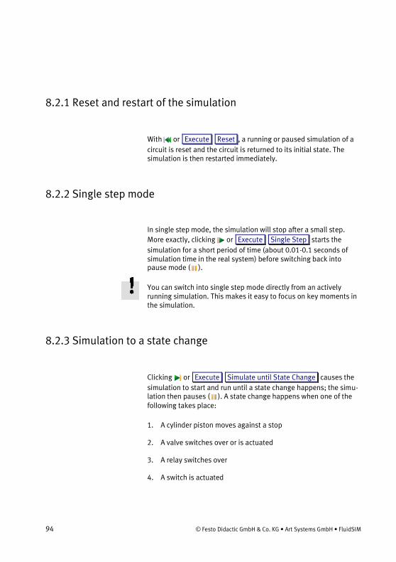
94 © Festo Didactic GmbH & Co. KG • Art Systems GmbH • FluidSIM
8.2.1 Reset and restart of the simulation
With or Execute Reset , a running or paused simulation of a
circuit is reset and the circuit is returned to its initial state. The simulation is then restarted immediately.
8.2.2 Single step mode
In single step mode, the simulation will stop after a small step.
More exactly, clicking or Execute Single Step starts the
simulation for a short period of time (about 0.01-0.1 seconds of simulation time in the real system) before switching back into pause mode ( ).
You can switch into single step mode directly from an actively running simulation. This makes it easy to focus on key moments in the simulation.
8.2.3 Simulation to a state change
Clicking or Execute Simulate until State Change causes the
simulation to start and run until a state change happens; the simu-lation then pauses ( ). A state change happens when one of the following takes place:
1. A cylinder piston moves against a stop
2. A valve switches over or is actuated
3. A relay switches over
4. A switch is actuated

© Festo Didactic GmbH & Co. KG • Art Systems GmbH • FluidSIM 95
You can switch into state change mode directly from an actively running simulation.
8.3 Simulating circuits you create yourself
This section assumes that you are already familiar with the basic concepts involved in creating circuits. If necessary, read the section Create a new circuit drawing" first.
Circuit diagrams can be created and modified in Edit Mode only. You can identify Edit Mode by the mouse arrow pointer .
8.3.1 Example with a pneumatic circuit
→ Create the circuit shown in the figure.

96 © Festo Didactic GmbH & Co. KG • Art Systems GmbH • FluidSIM
Figure 8/1: Simple pneumatic circuit
To define the valve’s actuation type, double click the valve. The valve’s property dialog opens.
→ Go to the “Configure Valve” tab. Then, in the top drop-down list on the left side, select a manual actuation with detenting. On the right side, click the “Spring-returned” field.
If required, you can also set the standard nominal flow rate of the valve.
Close the dialog box with &OK . As port “3” on the valve is only
needed as an air outlet, set a silencer there.
→ Double click the port.

© Festo Didactic GmbH & Co. KG • Art Systems GmbH • FluidSIM 97
A dialog box opens where you can select a Terminator by clicking the downward-pointing arrow to the right of the list and selecting the blanking plug or a silencer symbol.
→ Select the third symbol (the simple silencer) and close the dialog box.
The valve should now look like this:
Figure 8/2: Manually operated 3/2-way valve
Now try to simulate this circuit.
→ Start the simulation with (or with Execute Start or with
F9 ).
→ Move the mouse pointer onto the valve and click the valve with the pointing finger .

98 © Festo Didactic GmbH & Co. KG • Art Systems GmbH • FluidSIM
Figure 8/3: Simulated circuit
Once the cylinder has advanced, the pressure in the cylinder supply line must inevitably increase. This situation is detected by FluidSIM and the parameters are recalculated; the pressure at the com-pressed air supply increases to the set operating pressure.
→ Click the valve to make the cylinder retract.
In complex circuits, or for the transmission of high switching forces, valves may also be activated indirectly. In the following we will replace the direct manual activation of the valve with indirect pneumatic activation.
→ Activate Edit Mode with (or with Execute Stop or with
F5 ).

© Festo Didactic GmbH & Co. KG • Art Systems GmbH • FluidSIM 99
→ Select and delete the line that connects the cylinder and the valve.
→ Drag another 3/n-way valve onto the drawing area and open the valve configuration dialog box by double clicking (or by
Edit Properties... ). “Construct” a pneumatic valve (normally
closed), close the dialog box, put a silencer on port “3” again, and arrange the components as follows:
Figure 8/4: Circuit with unconnected components
→ Connect the new valve’s outlet port to the cylinder.
→ Draw a line from the outlet port of the manually operated valve to the control port of the pneumatic valve.
→ If necessary, drag the line segments until the drawing is ar-ranged clearly.

100 © Festo Didactic GmbH & Co. KG • Art Systems GmbH • FluidSIM
The circuit should now look something like this:
Figure 8/5: Circuit with indirect activation
→ Save this circuit with (or with File Save File ). FluidSIM
automatically opens the file selection box if the file did not al-ready exist; you can enter a file name in that box.
→ Start the simulation with and click the manually operated valve.
When you click a valve, the real behavior of the valve is simulated. In our example, the clicked valve is switched over and recalculation begins automatically. As a result, the indirectly activated pneumatic valve is switched and the cylinder advances.
FluidSIM not only animates the switching of manually actuated components, but nearly all components which have multiple states.

© Festo Didactic GmbH & Co. KG • Art Systems GmbH • FluidSIM 101
The following figure shows a 3/2-way valve in closed position and in open position:
Figure 8/6: Closed and open 3/2-way valve
When non-detenting components are clicked, they remain actuated as long as the mouse button is held down.
→ Stop the simulation and switch to Edit Mode. Select the state diagram from the component library and move it into the circuit window.
The state diagram records the quantity values for the most im-portant components and displays them in graph form.
→ Move the state diagram to a free space in the circuit drawing and drag and drop the cylinder onto the diagram.
A dialog box opens where you can select the quantity values you are interested in. In this instance, only the position is of interest, so you can remove the check marks for the other values (velocity, acceleration).
→ Start the simulation and observe the diagram.

102 © Festo Didactic GmbH & Co. KG • Art Systems GmbH • FluidSIM
Figure 8/7: Circuit with state diagram for the cylinder
→ Set the simulation to “ Pause ” and move the mouse pointer
onto the curve on the diagram.
If the mouse pointer rests on the diagram for a second, a box ap-pears showing the exact values for time and the relevant quantity value. If you move the mouse along the curve, the display alters accordingly, updating the values as the mouse pointer moves.

© Festo Didactic GmbH & Co. KG • Art Systems GmbH • FluidSIM 103
Figure 8/8: Display of the exact values in the state diagram
You can use multiple state diagrams in one window, and can also display multiple components in the same diagram. You can add a component to a state diagram by dragging it onto the diagram. A dialog will open, where you can select the quantity values to be logged and can assign different colors to them. Dragging onto the diagram again opens the dialog box again, allowing you to change your selection. If no quantity value is assigned to a component, it is not displayed in the diagram.
This concludes the example. Further editing and simulation con-cepts are described in the next section.
8.3.2 Example with a hydraulic circuit
→ Create the circuit shown in the figure.

104 © Festo Didactic GmbH & Co. KG • Art Systems GmbH • FluidSIM
Figure 8/9: Simple hydraulic circuit
To define the valve’s actuation type, double click the valve. valve’s property dialog opens.
→ Go to the “Configure Valve” tab. Then, in the top drop-down list on the left side, select a manual actuation and the valve bodies “Crosswise” and “Parallel”. Then on the right side, click the “Spring-returned” field.
If required, you can also set the hydraulic resistance of the valve.
Close the dialog box with &OK .
The valve should now look like this:

© Festo Didactic GmbH & Co. KG • Art Systems GmbH • FluidSIM 105
Figure 8/10: Manually operated 4/2-way valve
Now try to simulate this circuit.
→ Start the simulation with (or with Execute Start or with
F9 ).
Then all pressures and flow rates are calculated, the lines are colored, and the cylinder advances:

106 © Festo Didactic GmbH & Co. KG • Art Systems GmbH • FluidSIM
Figure 8/11: Simulated circuit
Once the cylinder has advanced, the pressure in the cylinder supply line should increase. This situation is detected by FluidSIM and the parameters are recalculated; the pressure on the pump side in-creases to the value predefined by the limit protection in the pump unit.
To limit the pressure to a lower value, you have to safeguard the pump unit with a pressure relief valve.
→ Activate Edit Mode with (or with Execute Stop or with
F5 ).

© Festo Didactic GmbH & Co. KG • Art Systems GmbH • FluidSIM 107
→ Drag a pressure relief valve and a second tank onto the draw-ing area.
→ If necessary, drag the line segments until the drawing is ar-ranged clearly.
The circuit should now look something like this:
Figure 8/12: Circuit with pressure relief valve
→ Save this circuit with (or with File Save File ). FluidSIM
automatically opens the file selection box if the file did not al-ready exist; you can enter a file name here.
→ Start the simulation with .

108 © Festo Didactic GmbH & Co. KG • Art Systems GmbH • FluidSIM
The cylinder advances. Once it reaches its stop, a new situation is created. This situation is detected by FluidSIM and the parameters are recalculated; the pressure relief valve opens, and the resulting distribution of pressure is shown:
Figure 8/13: Circuit with open pressure relief valve
FluidSIM not only animates the switching of manually actuated components, but nearly all components which have multiple states.
The following figure shows a pressure relief valve in closed position and in open position:

© Festo Didactic GmbH & Co. KG • Art Systems GmbH • FluidSIM 109
Figure 8/14: Closed and open pressure relief valve
Remember that manually operated valves and switches can be switched during Simulation Mode by clicking them with the mouse:
→ Move the mouse pointer onto the left-hand side of the direc-tional control valve.
The mouse pointer changes into a hand with pointing finger indicating that the valve can be switched over.
→ Click the left-hand side of the valve and hold down the mouse button.
When you click a valve with the mouse, the real behavior of the valve is simulated. In our example, the clicked valve is switched over and recalculation begins automatically. As a result, the pres-sure relief valve closes and the cylinder retracts. As soon as the cylinder reaches its left-hand stop, the pressure relief valve opens again.
When non-detenting components are clicked, they remain actuated as long as the mouse button is held down.
→ Stop the simulation and switch to Edit Mode. Select the state diagram from the component library and move it into the circuit window.
The state diagram records the quantity values for the most im-portant components and displays them in graph form.
→ Move the state diagram to a free space in the circuit drawing and drag and drop the cylinder onto the diagram.
A dialog box opens where you can select the quantity values you are interested in. In this instance, only the position is of interest, so

110 © Festo Didactic GmbH & Co. KG • Art Systems GmbH • FluidSIM
you can remove the check marks for the other values (velocity, acceleration).
→ Start the simulation and observe the diagram.
Figure 8/15: Circuit with state diagram for the cylinder
→ Set the simulation to “ Pause ” and move the mouse pointer
onto the curve on the diagram.
If the mouse pointer rests on the diagram for a second, a box ap-pears showing the exact values for time and the relevant quantity value. If you move the mouse along the curve, the display alters accordingly, updating the values as the mouse pointer moves.

© Festo Didactic GmbH & Co. KG • Art Systems GmbH • FluidSIM 111
Figure 8/16: Display of the exact values in the state diagram
You can use multiple state diagrams in one window, and can also display multiple components in the same diagram. You can add a component to a state diagram by dragging it onto the diagram. A dialog will open, where you can select the quantity values to be logged and can assign different colors to them. Dragging onto the diagram again opens the dialog box again, allowing you to change your selection. If no quantity value is assigned to a component, it is not displayed in the diagram.
This concludes the example. Further editing and simulation con-cepts are described in the next section.
8.3.3 Example with an electronic circuit
→ Create the circuit shown in the figure.

112 © Festo Didactic GmbH & Co. KG • Art Systems GmbH • FluidSIM
Figure 8/17: Simple electronic circuit
Now try to simulate this circuit.
→ Start the simulation with (or with Execute Start or with
F9 ).
Then all voltages and currents are calculated, and the potential from the positive terminal of the electrical power source to the pushbutton is colored.
→ Click the pushbutton and hold down the mouse button.
The current now flows through the pushbutton to the ground via the ammeter and the light:

© Festo Didactic GmbH & Co. KG • Art Systems GmbH • FluidSIM 113
Figure 8/18: Simulated circuit
The values for current and voltage can be read on the measuring devices. So far, the circuit is a purely electric circuit, strictly speak-ing. Now let’s add an electronic component: the diode.
→ Stop the simulation and switch to Edit Mode. Modify the circuit as shown in the figure and start the simulation.
Ensure that the diode is installed as shown. When you actuate the pushbutton, you will see that the potential only reaches as far as the diode:

114 © Festo Didactic GmbH & Co. KG • Art Systems GmbH • FluidSIM
Figure 8/19: Diode installed in reverse direction
→ Remove the diode and install it the other way around.
In this case rotating or mirroring the diode is not enough because while that would turn the component around, it would not change the line connections. That means that the lines would run through the component and the drawing would look correct.
FluidSIM detects drawing errors of this kind, highlights the critical sections, and issues a warning:

© Festo Didactic GmbH & Co. KG • Art Systems GmbH • FluidSIM 115
Figure 8/20: Warning of error in line layout
Once the diode is installed correctly, the current will flow through the diode and the light will light up:

116 © Festo Didactic GmbH & Co. KG • Art Systems GmbH • FluidSIM
Figure 8/21: Diode installed in forward direction
In practice it is important in electronics to pay attention to the exact currents and voltages. Electronic components are very sensitive and can be destroyed quickly if subjected to excessive loads.
Next, the pushbutton will be replaced by a potentiometer.
→ Stop the simulation and switch to Edit Mode. Modify the circuit as shown.

© Festo Didactic GmbH & Co. KG • Art Systems GmbH • FluidSIM 117
Figure 8/22: Simple circuit with a potentiometer
The potentiometer allows the resistance to be modified using a rotating or sliding controller. In FluidSIM you can click the potenti-ometer during the simulation and modify the resistance value as with a real potentiometer.
→ Start the simulation and display the amperages using View
Quantity Values... . Alternatively, you can also press the I key
repeatedly. Now click the potentiometer and watch how the current flow changes.
→ Stop the simulation and switch to Edit Mode. Select the state diagram from the component library and move it into the circuit window.
The state diagram records the quantity values for the most im-portant components and displays them in graph form.
→ Move the state diagram to a free space in the circuit drawing and drag and drop the ammeter onto the diagram.
A dialog box opens where you can select the quantity values you are interested in. In this instance, only the amperage is of interest.

118 © Festo Didactic GmbH & Co. KG • Art Systems GmbH • FluidSIM
→ Start the simulation, vary the resistance value of the potenti-ometer, and observe the diagram.
Figure 8/23: Circuit with state diagram for the ammeter
→ Set the simulation to “ Pause ” and move the mouse pointer
onto the curve on the diagram.
If you move the mouse along the curve, the display alters accord-ingly, updating the values as the mouse pointer moves. If you move

© Festo Didactic GmbH & Co. KG • Art Systems GmbH • FluidSIM 119
the mouse along the curve, the display alters accordingly, updating the values as the mouse pointer moves.
Figure 8/24: Display of the exact values in the state diagram
You can use multiple state diagrams in one window, and can also display multiple components in the same diagram. You can add a component to a state diagram by dragging it onto the diagram. A dialog will open, where you can select the quantity values to be logged and can assign different colors to them. Dragging onto the diagram again opens the dialog box again, allowing you to change your selection. If no quantity value is assigned to a component, it is not displayed in the diagram.
This concludes the example. Further editing and simulation con-cepts are described in the next section.

Advanced concepts in simulating and creating circuits
120 © Festo Didactic GmbH & Co. KG • Art Systems GmbH • FluidSIM
Chapter 99. Advanced concepts in simulating and creating circuits
This section describes advanced concepts and functions for simula-tion and circuit creation in FluidSIM.
9.1 Adjusting the component parameters
Most of the symbols in FluidSIM’s component library are basic symbols representing various different versions of a component. You can use the properties dialog box to customize the compo-nent’s parameters, size, characteristic curves etc..
In Expert Mode there are sometimes many more parameters
available, depending on the component. These allow you to modify, for example, spring forces, friction, or effective area. These parame-ters are hidden in the standard mode. To avoid having to switch Expert Mode on and off continuously, you can use the “Show all settings” option to temporarily display all parameters or to hide the advanced settings.
→ Drag a one-way flow control valve (throttle check valve) onto the drawing area and open the properties dialog box by double clicking.
You can access the adjustable parameters on the “Component Parameters” tab.
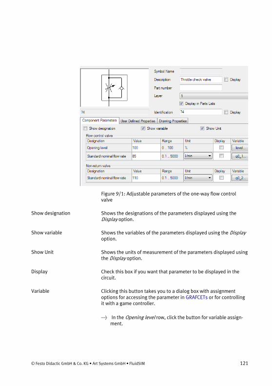
© Festo Didactic GmbH & Co. KG • Art Systems GmbH • FluidSIM 121
Figure 9/1: Adjustable parameters of the one-way flow control valve
Shows the designations of the parameters displayed using the Display option.
Shows the variables of the parameters displayed using the Display option.
Shows the units of measurement of the parameters displayed using the Display option.
Check this box if you want that parameter to be displayed in the circuit.
Clicking this button takes you to a dialog box with assignment options for accessing the parameter in GRAFCETs or for controlling it with a game controller.
→ In the Opening level row, click the button for variable assign-ment.
Show designation
Show variable
Show Unit
Display
Variable

122 © Festo Didactic GmbH & Co. KG • Art Systems GmbH • FluidSIM
Figure 9/2: Variable and controller assignment of a parameter
This is the standard, complete variable name. It is made up of the identification entered by you and the internal parameter name. You can use this variable name to access the parameter in GRAFCETs in order to query it or modify its value.
If you do not like the predefined variable name, you can enter your own name for it here. Note that this alias has to be unique across the entire page or project. FluidSIM issues a warning if an alias name is entered twice.
Predefined variable
User-defined alias

© Festo Didactic GmbH & Co. KG • Art Systems GmbH • FluidSIM 123
As described in the "Adjusting component parameters during the simulation" section, many component parameters can be altered with the mouse during the simulation. FluidSIM also offers the option of controlling parameters via connected game controllers (e.g. Microsoft Xbox controller). This is especially practical when you need to modify several parameters at the same time during a simulation.
Here you can define which axis you want to use to control the parameter during the simulation. To assign an axis, simply click in the field and briefly actuate the desired controller axis. FluidSIM then enters the desired axis.
This value determines how much movement of the controller axis is required to trigger a signal. This prevents unintended modification of values from very small movements of the fingers.
Sometimes you may wish to use the game controller to control only a certain range. This can be necessary above all because the con-trol levers on most controllers spring back to their zero position automatically as soon as they are released. Using the mouse to-gether with the straight line on the graph, you can interactively determine how the controller position relates to the parameter.
Controller assignment is not available for the simulation variables calculated by FluidSIM (piston positions, velocities, pressures, flow rates, etc.) because these variables only permit read access. Simi-larly, these variables cannot be assigned in GRAFCETs. FluidSIM displays a warning if an attempt is made to modify a simulation variable.
Simulation variables therefore have only the option of variable assignment.
Controller assignment
Axis
Dead-zone
Range

124 © Festo Didactic GmbH & Co. KG • Art Systems GmbH • FluidSIM
Figure 9/3: Variable assignment of a simulation parameter
9.2 Special settings for cylinders
To adapt a cylinder, drag a representative cylinder into the circuit and open the properties dialog box. It contains settings that you can use to determine the appearance and function of the compo-nent. See section "Configure cylinders" for the basic functions for configuring the cylinder properties.
9.2.1 Cylinder friction and cylinder mass
If the options “Show all settings” and “Enter manually” are select-ed, you can specify parameters defining a velocity-dependent characteristic curve and the mass moved by the cylinder. If you select “Calculate automatically”, an heuristic is applied which calculates the settings on the basis of the cylinder dimensions.
Clicking an input field in the “Cylinder friction” section activates a “...” button that can be used to open a dialog box containing a graph displaying the cylinder friction as a function of the cylinder velocity.

© Festo Didactic GmbH & Co. KG • Art Systems GmbH • FluidSIM 125
Figure 9/4: Friction curve of a pneumatic cylinder
9.2.2 External load and friction

126 © Festo Didactic GmbH & Co. KG • Art Systems GmbH • FluidSIM
Figure 9/5: External load on the cylinder
Enter here the mass of the load that you want the cylinder to move. The mass of the cylinder piston and piston rod is calculated auto-matically by FluidSIM from the entered cylinder dimensions, so the mass entered here refers only to the external load. In particular, an entry of “0” does not mean that the moving parts in the cylinder have no mass.
The static friction and sliding friction define the friction of the moving load on a surface. The internal friction in the cylinder is calculated automatically by FluidSIM from the entered cylinder dimensions. If the load is lifted or pulled without coming into con-
Moving mass
Friction

© Festo Didactic GmbH & Co. KG • Art Systems GmbH • FluidSIM 127
tact with a surface, enter “0” for both values. In practice it is very difficult to arrive at reliable values for friction. FluidSIM therefore offers set friction coefficients for some combinations of materials, to provide a rough guide. If you compare other tables of friction values, you will notice that the specifications (usually measured in experiments) vary greatly from table to table. You should therefore be cautious when interpreting the results of simulations influenced by friction. Nonetheless, varying the friction values does allow you to see clearly the physical effects of static and sliding friction. Note also that the mounting angle influences the friction force from the moved load. You can adjust the mounting angle on the “Component Parameters” tab.

128 © Festo Didactic GmbH & Co. KG • Art Systems GmbH • FluidSIM
9.2.3 Force profile
Figure 9/6: Force profile of the cylinder
If you want a constant force to be applied over the entire range of cylinder movement, select this option and enter a force.
Select this option if you want the force to change depending on the cylinder’s position. By clicking the mouse in the graph field, you can interactively set reference points which will be interpolated to form a line. Alternatively, you can select an existing reference point
Constant force
Apply force profile

© Festo Didactic GmbH & Co. KG • Art Systems GmbH • FluidSIM 129
and numerically enter the two values in the input fields for the piston position and the corresponding force.
You can use the sliders to adjust the displayed value ranges for position and force. As the force on the y-axis covers an especially wide numerical range, it is advisable to start by restricting that interval so that the shape of the curve can be seen clearly.
Select this option if you want to apply the same force profile for advancing and retraction. Otherwise, remove the checkmark and enter separate force profiles on the tabs “Extraction” and “Retrac-tion”.
Retraction = Extraction

130 © Festo Didactic GmbH & Co. KG • Art Systems GmbH • FluidSIM
9.2.4 Actuating labels
Figure 9/7: Actuating labels on the cylinder
Here you can create new actuating labels or modify existing ones. This dialog box is identical to the one that opens when you double click an distance rule.
In addition to the actuating labels you can also enter a special label for a continuous displacement encoder or select from the list of counterparts already present in the project.
Displacement encoder

© Festo Didactic GmbH & Co. KG • Art Systems GmbH • FluidSIM 131
9.3 Special settings for directional control valves
To adapt a directional control valve, drag a representative cylinder into the circuit and open the properties dialog box. It contains settings that you can use to determine the appearance and function of the component. See section "Configure a way valve" for the basic functions for configuring the valve properties.
9.3.1 Hydraulic resistance
For hydraulic valves, you can adjust the hydraulic resistance. In practice the hydraulic resistance is often given by a curve or a pair of values (pressure drop/flow rate). In the field “Hydraulic re-sistance” you can either enter a specific value or alternatively click the “...” button. That takes you to a dialog box where you can define the parabola either by interactively clicking in the graph field or by entering a pair of values.

132 © Festo Didactic GmbH & Co. KG • Art Systems GmbH • FluidSIM
Figure 9/8: Hydraulic resistance curve
9.4 Additional simulation functions
This section describes additional functions for the simulation of circuit diagrams.

© Festo Didactic GmbH & Co. KG • Art Systems GmbH • FluidSIM 133
9.4.1 Simultaneous actuation of several components
So that you can actuate multiple pushbuttons or spring-returned valves at the same time, you can put them in a permanently actuat-ed state. You can permanently actuate a pushbutton (or valve with manual actuation) by clicking it with the mouse while pressing the
Shift key. You can release this permanent actuation by clicking
once on the component.
Sometimes it may be necessary for multiple actuated objects to be released at the same time. In that case, when clicking the object,
hold down the Ctrl key instead of the Shift key. The switched
components then remain in the actuated state until you release the
Ctrl key again, at which time all the objects actuated in this way
return to their initial position simultaneously.
For more complex switching operations or continuous adjustments, we recommend using a game controller. For more details, see "Adjusting the component parameters".
9.4.2 Simulation of individual pages and entire projects
In FluidSIM it is possible for multiple circuits to be open at the same time. Circuits whose pages belong to a project are simulated as an entire system. This is practical if, for example, you want to create the hydraulic or pneumatic part and the electrical part on separate pages. You can also divide large drawings across multiple pages and define the line connections using interruption points. When a circuit belonging to a project is simulated, all the other pages of the project switch into Simulation Mode as well when the simulation is started. While the simulation is running, it is therefore not possible to edit any pages belonging to the open project.
In contrast, if pages that do not belong to the project are edited or simulated, the editing or simulation always applies only to the

134 © Festo Didactic GmbH & Co. KG • Art Systems GmbH • FluidSIM
currently active circuit window. In such cases, it is therefore possi-ble to simulate one circuit while editing another.
9.5 Displaying quantity values
The numerical values for all or some quantity values in a circuit can be displayed even without measuring devices.
→ In the View menu, click Quantity Values... to open the
dialog box for the display of quantity values:

© Festo Didactic GmbH & Co. KG • Art Systems GmbH • FluidSIM 135
Figure 9/9: Dialog box for adjusting the quantity values display
Here you can define how every quantity value listed (“Velocity”, “Pressure”, etc.) will be displayed.
For the display of pressure values, flow rates, and forces, you can choose between different units of measurement. These settings take effect when quantity values are displayed at connectors and components and on state diagrams.
Do not display any values for this quantity value.
Display values only at connection points previously selected by the user.
None
Individual

136 © Festo Didactic GmbH & Co. KG • Art Systems GmbH • FluidSIM
Display all values for this quantity value.
Activate this option if you also want the unit of measurement to be displayed for the quantity values.
You can use the key in the “Shortcut” column to switch between
the display types “ None ”, “ Individual ” and “ All ” for that
particular quantity value without having to open the dialog box.
Proceed as follows to select connection points for the display of individual quantity values:
→ Open a circuit.
→ In Edit Mode, double click a component connector, or select
the menu item Edit Properties... .
The dialog box for the connector’s settings then opens. In the “Display quantity values” field, you can choose which quantity
values are to be displayed at that connector when the “ Individual
” option is activated for that parameter in the dialog box for quanti-ty values display.
9.5.1 Display of direction of quantity values in FluidSIM
Vectorial quantity values are characterized by their quantity and their direction. In circuit diagrams, the direction is displayed at the component connectors by a mathematical sign (“+” = into a com-ponent, “–” = out of a component). If the amount of the quantity value is close to zero, the exact numerical value is not displayed. Instead, “> 0” is displayed for a small positive value and “< 0” for a small negative value.
In the case of fluidic flows, the direction is also indicated by an arrow in the middle of the line segment. The visual impression is reinforced by conveyor-belt-style animation of the lines.
All
Display measurement units

© Festo Didactic GmbH & Co. KG • Art Systems GmbH • FluidSIM 137
9.6 Displaying state diagrams
The state diagram records the quantity values for the most im-portant components and displays them in graph form. Quantity values or output variables all those values calculated by FluidSIM during the simulation or set by the user, such as: position, velocity, acceleration, force, switching position, pressure, flow rate, opening level, revolutions/rpm, voltage, current, digital state, etc.
You can use multiple state diagrams in one window, and can also display multiple components in the same diagram. You can add a component to a state diagram by dragging it onto the diagram. A selection dialog box will open, where you can select the quantity values to be logged and can assign different colors to them. Drag-ging onto the diagram again opens the dialog box again, allowing you to change your selection.
→ In Edit Mode, double click a state diagram, or select the menu
item Edit Properties... .
The following dialog box will open:

138 © Festo Didactic GmbH & Co. KG • Art Systems GmbH • FluidSIM
Figure 9/10: Dialog box for the state diagram
Here you can enter the start and end times of the interval during which you want the quantity values to be logged. You do not nec-essarily need to know before starting the simulation the times at which the important events will occur; you can always change the display interval as desired after the simulation because FluidSIM always logs all values internally for the entire simulation period. If you select the “Adjust automatically” field, the entered limits are ignored and the time axis is scaled so that the entire simulation time is displayed. Activate the “Scroll automatically” field if you want the diagram to display the last n seconds. In this case, the time axis will be displaced toward the left-hand side once the simulation period exceeds the defined time window. In the input field, you can specify the number of seconds to be displayed in the time window.
Here you can select which columns you want to be displayed at the left-hand side of the diagram. You can choose the columns “De-scription”, “Identification”, and “Quantity value” in any combina-tion.
Display interval
Diagram columns

© Festo Didactic GmbH & Co. KG • Art Systems GmbH • FluidSIM 139
If you wish, FluidSIM can create a log file of the quantity values. Activate this option by entering the full path for the file in the input field and select a suitable time increment. Please note that entering very small increments may result in a very large volume of data. You may need to reduce the simulation time or increase the time increment.
Defines the color of the diagram.
Defines whether the entire area is filled with the chosen color or just the border of the diagram.
In this drop-down list, you define the Layer of the diagram. You can set the Layer by clicking the downward-pointing arrow to the right of the list and selecting a layer. Depending on the setting for draw-ing layers, the rectangle might not be displayed or might not be able to be edited. In order to see the object or change its settings, you have to temporarily activate the drawing layers with menu item
View Drawing Layers... .
This list contains all the quantity values displayed in the diagram. Every component is listed together with its identification, and all its output variables are listed below it. Every variable can be selected and deselected with a checkmark. Once you have marked a varia-ble, you can use the buttons at lower right to define the color, line
style, and line thickness for it. You can use Add to select the
components you want. Delete deletes the marked component
together with its quantity values, and Find Target... takes you to
the relevant component in the circuit.
9.7 Coupling hydraulics, pneumatics, electrics and mechanics
All three available technology versions, FluidSIM-P, FluidSIM-H and FluidSIM-E, allow you to create basic electrical circuits. In the pneumatics and hydraulics versions, they are used primarily to control the fluidic components. Because these simple electrical components are simulated completely with full physical accuracy, just as much as the electronic components are, they can be used
Log file
Color
Fill Area
Layer
Quantity values

140 © Festo Didactic GmbH & Co. KG • Art Systems GmbH • FluidSIM
and interchanged across all FluidSIM versions and can be combined with the electronic components in FluidSIM-E.
The following figure shows a small example:
Figure 9/11: Simple electrical circuit
→ Create this circuit on your computer.
→ Start the simulation and observe that the indicator light lights up.
There are electrical components that link electrical circuits with pneumatic or hydraulic circuits. These include switches that are operated pneumatically or hydraulically, and solenoids for the control of valves.
As the electrical circuit is drawn separately from the fluidic circuit, you need a way of creating a definite link between electrical com-ponents (e.g. a valve solenoid) and fluidic components (e.g. a certain valve position). One way of doing this is with so-called labels.

© Festo Didactic GmbH & Co. KG • Art Systems GmbH • FluidSIM 141
A label has a specific name and can be assigned to a component. If two components have labels with the same name, they are con-nected even if there is no visible line drawn between them.
You can enter the name for a label in a dialog box which you open either by double clicking the component or by selecting the compo-
nent and clicking Edit Properties... . With electrically operated
valves (solenoid actuated), the labels are entered on the left and the right by double clicking the appropriate “connector”, as op-posed to clicking in the middle of the component.
The following example illustrates how labels are used in FluidSIM.
→ Activate Edit Mode with or with Execute Stop .
→ Expand the circuit as shown in the following figure:

142 © Festo Didactic GmbH & Co. KG • Art Systems GmbH • FluidSIM
Figure 9/12: Simple electro-pneumatic circuit
So that the valve can be controlled by the solenoid, these compo-nents need to be linked using labels.
→ Double click the valve solenoid or select the solenoid and click
Edit Properties... .
The following dialog box appears:

© Festo Didactic GmbH & Co. KG • Art Systems GmbH • FluidSIM 143
Figure 9/13: Dialog box for the valve solenoid
This text field is for entering a label name. A label name can be up to 32 characters long and can contain numerals and special charac-ters as well as letters.
→ Enter a name (e.g. “Y1”) for this label.
→ Double click the outside of the solenoid on the valve to open the dialog box for the label name.
→ Enter the same label name there as for the solenoid (“Y1”).
The solenoid is now connected to the valve.
In reality, the valve solenoid would not be activated directly via the switch but via an intermediate relay. This is left out here for the sake of simplicity.
→ Start the simulation.
The electrical current and the pressure and flow distribution are calculated, and the resulting pressures are shown in color.
If you want to view the exact values for the quantity values, you can
activate them in the dialog box accessible via View Quantity
Values... . The activated quantity values are shown at the compo-
nent connection points. For more detailed information about this, see "Displaying quantity values".
Identification

144 © Festo Didactic GmbH & Co. KG • Art Systems GmbH • FluidSIM
→ Operate the electrical switch.
The valve then switches over and the cylinder advances:
Figure 9/14: Simulation of the electro-pneumatic circuit
In addition to manual actuation or electrical control, some valves can also be switched over mechanically by the piston rod of a cylinder or by a permanent magnet on the piston. Mechanical linkages like this are created in the same way as those with electri-cal components: The connection is established by applying a label to the cylinder’s distance rule and another to the mechanical “con-nector” on the valve.
→ Drag a configurable valve into a circuit window and specify a mechanical actuation (e.g. the stem).

© Festo Didactic GmbH & Co. KG • Art Systems GmbH • FluidSIM 145
Figure 9/15: Valve with mechanical actuation
→ Double click the end of the stem.
A dialog box will open in which you can enter a label. If you enter the same label on the cylinder’s distance rule, the valve will be actuated mechanically when the cylinder’s piston rod reaches the specified position.
A special instance of this type of linkage is the connection of a cylinder to a displacement encoder. You can use such connections to construct closed-loop control systems in combination with proportional valves, for example. Further information about propor-tional control systems can be found in section "Open-loop and closed-loop control by using continuous valves".
→ Double click a cylinder.
A dialog box will open in which you can adjust the cylinder’s prop-erties. Go to the “Actuating labels” tab.

146 © Festo Didactic GmbH & Co. KG • Art Systems GmbH • FluidSIM
Figure 9/16: Cylinder configuration dialog box
→ Enter a label under “Displacement encoder”.
→ Add the displacement encoder from the component library to the circuit and double click to open the properties dialog box. Enter the same label there as you entered for the cylinder.

© Festo Didactic GmbH & Co. KG • Art Systems GmbH • FluidSIM 147
Figure 9/17: Linking the displacement encoder to the cylinder
The displacement encoder returns a voltage at its output which is proportional to the piston position of the linked cylinder. When the cylinder is fully retracted, this voltage will be the set minimum; when the cylinder is fully advanced, it will be set maximum.
9.7.1 Display styles for labels
As with component designations, it is often desirable to surround labels with a rectangular frame. You can select this in the basic
settings for fluidic and electrical labels in the Options... menu.
However, you can also set the frame for specific texts to be differ-ent from the standard frame. To do so, double click the specific text:

148 © Festo Didactic GmbH & Co. KG • Art Systems GmbH • FluidSIM
Figure 9/18: Dialog box for setting the text frame
Under Text Attributes you can set the option Frame Text.
FluidSIM automatically positions the labels so that they appear at an appropriate position near the component or connector. Howev-er, you can also move the labels using the mouse or the keyboard. To do so, click the label and drag it to the desired position. To modify the position with the keyboard, select the label (or the associated connector) and move the label using the cursor keys.
If you have inadvertently moved a label text so far that you cannot tell which component it belongs to, you can double click the label to open the properties dialog box and then activate the associated
component with Find Target... .
9.8 Operating switches
This section describes how switches can be actuated by cylinders, relays, pressure, or by other switches.

© Festo Didactic GmbH & Co. KG • Art Systems GmbH • FluidSIM 149
9.8.1 Switches at cylinders
Limit switches, proximity switches, and mechanically actuated valves can be activated by the piston of the cylinder. To make this possible, first you have to place a distance rule on the cylinder so that the switches can be positioned.
→ Drag the cylinder onto the drawing area and open its proper-ties by double clicking. Go to the “Actuating labels” tab and en-ter a label along with the start and end positions.
When you close the dialog box, the distance rule will appear auto-matically above the cylinder. You can move or copy the distance rule from one cylinder to another. When the distance rule comes close to a cylinder, it slots automatically into the correct position.
The correct position for a distance rule depends on the cylinder type. Distance rules can be positioned over the cylinder housing, in front of the cylinder housing (next to the advanced piston rod) or in both positions at the same time:
Figure 9/19: Examples of distance rule positions
To modify the labels or positions or to add more, you can either open the properties for the associated cylinder or enter these details directly on the distance rule.
→ Double click the distance rule.
The following dialog box appears:

150 © Festo Didactic GmbH & Co. KG • Art Systems GmbH • FluidSIM
Figure 9/20: Dialog box for the distance rule
The text fields in the left-hand column are used to enter the label names of proximity switches or limit switches in the electrical circuit that you want the cylinder piston to actuate.
The text fields in the right-hand columns define the exact start and end positions of the switches on the cylinder.
→ Enter “Y1” as the label in the first row and enter 35 for both the start and end positions, and close the dialog box by clicking
“ &OK ”.
A dash with the label name will appear immediately at the corre-sponding position under the distance rule:
Figure 9/21: Cylinder with distance rule
This means that this cylinder will activate the switch or valve la-beled “Y1” once its piston has moved 35 mm, assuming that the same label was entered on the switch in the electrical part of the circuit or on the mechanical “connector” of the valve.
Label
Position

© Festo Didactic GmbH & Co. KG • Art Systems GmbH • FluidSIM 151
Once the cylinder in the above example passes the 35 mm position, the switch will drop out again. If you want the actuation to be maintained over a longer distance, enter the start and end posi-tions accordingly in the dialog box.
To place labels on electrical switches, double click the component. Valves with mechanical actuation have a special connector for this purpose, which may be on the end of the stem or in the center of the roller, for example. If there is already a label on the component or connector, you can also double click the label directly and then
click Find Target... to open the corresponding dialog box for
editing the label.
9.8.2 Relays
A relay or solenoid can be used to actuate multiple switches or contacts simultaneously. It is of course necessary to link the relay to the relevant switches. Therefore in FluidSIM, relays too have labels, which can be used to define an association with switches in the usual way. When you double click a relay, the dialog box for the label name will open.
The following figure shows an electrical circuit diagram in which a relay simultaneously actuates two break switches and two make switches:
Figure 9/22: Relay with linked switches
In addition to the simple relay, there are also relays with switch-on delay, relays with switch-off delay, and counting relays. They en-sure that the linked switches are not actuated until a defined time or number of pulses is reached. With these relays too, double clicking will open the corresponding dialog boxes for entering the values.

152 © Festo Didactic GmbH & Co. KG • Art Systems GmbH • FluidSIM
9.8.3 Coupling mechanical switches
The mechanical linkage of mechanical (manually operated) switch-es is accomplished in FluidSIM by assigning a label. If multiple mechanical switches have the same label, actuating one of them will cause all the identically labeled switches to be actuated with it.
9.8.4 Automatic switch altering
FluidSIM identifies delay switches, limit switches, and pressure switches by their method of installation and by their labels and automatically adds the corresponding symbol to the switch in the electrical circuit: for switch-on delayed, for off-delayed, for mechanical actuated switches and for pressure switches. In the case of switches actuated by the cylinder piston, you can choose how they are displayed in the properties dialog box for the closer, opener, and changeover:

© Festo Didactic GmbH & Co. KG • Art Systems GmbH • FluidSIM 153
Figure 9/23: Dialog box for general electrical switches
This means that special symbols do not need to be used for these switches in FluidSIM. The simple switch symbols can be used instead:
Figure 9/24: Simple switch symbols
9.9 Adjusting component parameters during the simulation
Most components have parameters that can be adjusted in Edit Mode. Some of these components have already been discussed in earlier sections.

154 © Festo Didactic GmbH & Co. KG • Art Systems GmbH • FluidSIM
You can open the dialog box for adjusting the parameters by dou-
ble clicking or with Edit Properties... .
Several components can be adjusted during the simulation in the same way as they would be in reality. For example, the operating pressure of the compressed air supply, the delivery rate of the pump, the opening level of the throttle valve, or the resistance of the potentiometer can be altered continuously. To do this, you do not need to open the properties dialog box and then close it with
&OK ; all you need to do is click once on the component to open a
window with sliders. Your changes take effect on the simulation immediately. As soon as you click another component or an empty space in the window, the dialog window with the sliders disappears automatically.
In Simulation Mode, when you move the mouse over a component that allows such real-time adjustments, the mouse pointer changes
into the slider symbol .
Figure 9/25: Adjusting the opening level during the simulation
For precision adjustment, some sliders allow you to select the control range. However, you can also enter the numeric value directly as a number in the input field.
Most parameters can also be controlled using a game controller. For details, see "Adjusting the component parameters".

© Festo Didactic GmbH & Co. KG • Art Systems GmbH • FluidSIM 155
9.10 Settings for simulation
In the Options... menu, basic parameters and options for the
simulation can be set under Simulation, Environment parameters, Fluid properties, and Sound.
Note that these settings are only used if no others are defined in the page or project properties. Newly created pages and projects
are preset with the standard values set under Options... .
9.11 Use of the EasyPort-hardware
FluidSIM can directly address EasyPorts connected to the serial ports of the PC. No additional drivers or auxiliary programs are required. These days, however, serial ports are rare outside indus-trial environments. To use the EasyPort via a USB cable, you may require drivers that you will find on the installation DVD and which you can also download online from Festo Didactic GmbH & Co. KG.
The EasyPort hardware is linked to the components in FluidSIM via special electrical input/output components, which each have either eight digital inputs/outputs or two analog outputs/four analog inputs.
The EasyPort hardware can also be addressed using DDE and OPC communication. This allows you to control even remote EasyPort modules that are not connected locally (e.g. via a network connec-tion). However, if the EasyPort modules are connected directly to the simulating PC, it is recommended to set up the direct connec-tion.
→ Drag a digital input or output component from the component library into a circuit window and open the properties dialog box
by double clicking or via the menu item Edit Properties... .
The following dialog box will open:

156 © Festo Didactic GmbH & Co. KG • Art Systems GmbH • FluidSIM
Figure 9/26: Dialog box for the EasyPort components
Here you can set the serial port by which the hardware is connected to the PC, which EasyPort module and port number is assigned to the input/output component. If you do not know the exact number of the serial port, leave the setting as “Automatically”. FluidSIM then searches all COM ports for connected EasyPorts.
Older EasyPorts are fitted as standard with only a serial port, of the kind used for many years on PCs and also in industrial applications. Modern PCs and especially portable computers, however, increas-ingly do not feature this connection. Nonetheless the serial port interface can be retrofitted easily using an inexpensive USB-to-serial converter, allowing the EasyPort to be connected and operat-ed anyway. The converter’s software does this by setting up a virtual COM port, which is assigned a number higher than the physically existing ports (usually COM 5). The hardware can be addressed in the usual way via this virtual port.
Defines the color of the connection indicators for the input/output component when the EasyPort connection is active and when the connection is not present or is disrupted.
With the analog interface components, you can select the voltage range. This can be either from 0V to 10V or from -10V to 10V.
Direct EasyPort connection
Connector color
Voltage range

© Festo Didactic GmbH & Co. KG • Art Systems GmbH • FluidSIM 157
If FluidSIM does not find any EasyPort hardware at the start of the simulation, a corresponding warning is issued. You can start the simulation anyway, but if you do so FluidSIM will not make any further attempts to find EasyPorts until the simulation is closed and restarted. If, on the other hand, the connection is terminated while the simulation is running (e.g. by inadvertently pulling out the connecting cable), the simulation will continue to run without the EasyPort link, but FluidSIM will attempt to restore the connection. As soon as the hardware is once again available at the set port, the connection is restored and the simulation continues with EasyPort communication.
9.12 OPC and DDE communication with other applications
FluidSIM is capable of exchanging data with other applications, allowing it to work together with a PLC, for example. A prerequisite for this link is that the other application has an “OPC interface” or a “DDE interface”. The link is established using the same interface components as for the use of FluidSIM with the EasyPort.
→ Drag an input or output component from the component library into a circuit window and open the properties dialog box
by double clicking or via the menu item Edit Properties... .
The following dialog box will open:

158 © Festo Didactic GmbH & Co. KG • Art Systems GmbH • FluidSIM
Figure 9/27: Dialog box for the OPC components
→ In the “Connect EasyPort via” list, select the “OPC connection” option.
Enter the OPC server here or press the Pick... button and select it
from the list.
Enter the data item here or press the Pick... button and select it
from the list.
In order to establish communication via a DDE interface, first en-sure that the DDE interface is active. You can do this with the global option under DDE Connection.
→ In the “Connect EasyPort via” list, select the “DDE connection” option.
OPC server
Item

© Festo Didactic GmbH & Co. KG • Art Systems GmbH • FluidSIM 159
Figure 9/28: Dialog box for the DDE components
This is the server name that FluidSIM uses when it registers in the system as a DDE server. As the server name is a global setting, it
cannot be changed directly in this dialog box. Pressing the Global
DDE server name... button takes you to the options dialog box
where you can change the server name for the entire system.
Here, enter the “topic” via which you would like to address the components.
Here, enter the label or the “item” via which you would like to address the components.
9.13 Open-loop and closed-loop control by using continuous valves
In addition to simple directional control valves, which only have discrete switching positions, FluidSIM also offers some continuous valves. These are characterized by their ability to adopt a continu-ous range of intermediate positions. Like electrically actuated
Server
Topic
Label

160 © Festo Didactic GmbH & Co. KG • Art Systems GmbH • FluidSIM
directional control valves, these components are controlled via a proportional amplifier or via a valve solenoid. These valves, howev-er, are represented by special symbols:
Figure 9/29: Proportional valve solenoid and amplifier
The separate proportional valve solenoid is used for position-controlled continuous valves where the control and amplifier com-ponent is built into the valve.
If you inadvertently use a label to link a directional control valve to a proportional valve solenoid, or a proportional valve to a simple valve solenoid, FluidSIM issues a warning.
The following two sections provide a brief introduction to the options for open-loop control and closed-loop control with FluidSIM.
The term “open-loop control” means that an output variable changes as a function of an input variable. In this specific case, the voltage on the proportional valve solenoid or amplifier represents an input variable. The valve piston of the proportional valve is shifted in a particular direction to a greater or lesser distance as a function of the value (and the direction) of the electrical current caused by that voltage (by means of an amplifier). This piston displacement is the output variable. If the pressure at the valve port is constant, the flow rate can be controlled in this way. If, on the other hand, the flow rate is constant, the pressure drop will change as a function of the opening level, determined by the valve position.
The term “closed-loop control” is used when the output variable (or a quantity value affected by it) is used in turn as the input variable. It is also quite possible for multiple output variables (and quantity values dependent on them) to be combined together with addition-al input variables, using a calculation rule. A classic example is position control, where a cylinder needs to move to a certain posi-

© Festo Didactic GmbH & Co. KG • Art Systems GmbH • FluidSIM 161
tion. The valve is activated electrically so that the cylinder moves. The cylinder’s position (resulting from the movement caused by the valve setting) is used in turn as an input variable, to determine the deviation between the cylinder’s position and its setpoint position. Once the cylinder has reached its target position, the deviation is 0 and the valve returns to its mid-position (closed position). The cylinder thus comes to a halt. If inertia or external disruption caus-es the cylinder to move past its target, the valve switches over to the other side, reversing the flow direction, and the cylinder moves back. This is the simplest form of closed-loop control, known as “P control” (proportional control).
9.13.1 Open-loop control in pneumatics
In order to understand how the continuous components function, please construct the following circuit (power supply, function generator, voltmeter, proportional valve solenoid, regulating valve):
Figure 9/30: Simple open-loop control of the regulating valve
Do not forget to fit silencers on the valve’s five pneumatic ports, in order to prevent warnings from FluidSIM.
→ Start the simulation and observe the regulating valve.
The function generator generates a signal between 0 and 10 volts. This varying voltage is converted by a proportional amplifier in the valve into a corresponding current that actuates the proportional

162 © Festo Didactic GmbH & Co. KG • Art Systems GmbH • FluidSIM
valve solenoid, so that the valve connected to it is shifted to either side to the maximum extent according to the signal voltage applied.
To switch over the valve to a lesser extent, the valve requires a lesser maximum voltage. You can set that by opening the proper-ties dialog box for the function generator, by double clicking.
Figure 9/31: Properties dialog box for the function generator
→ Enter 2 as the “Amplitude”, close the dialog box, and restart the simulation.
The voltage will now vary between 3 and 7 volts. As a result, the valve will still shift symmetrically, but with less displacement from the mid-position.
→ Open the function generator properties again and set 3 as the y offset.
The function generator now supplies a voltage between 1 and 5 volts, with the valve moving further to the left than to the right.
→ Open the function generator properties again and set “Con-stant” as the signal type.

© Festo Didactic GmbH & Co. KG • Art Systems GmbH • FluidSIM 163
The sliders of the function generator for “Frequency” and “Ampli-tude” have no function when the signal type is set to “Constant”. This allows us to use it to simulate a manually adjustable potenti-ometer.
→ Start the simulation and click the function generator (with a single click).
A window opens showing the sliders of the function generator.
Figure 9/32: Adjusting the function generator during the simulation
→ Change the y offset very gradually, while observing how the valve moves as a function of the slider setting.
9.13.2 Open-loop control in hydraulics
In order to understand how the continuous components function, please construct the following circuit (power supply, function generator, voltmeter, proportional valve solenoid, regulating valve):

164 © Festo Didactic GmbH & Co. KG • Art Systems GmbH • FluidSIM
Figure 9/33: Simple open-loop control of the regulating valve
Do not forget to fit blanking plugs on the valve’s four hydraulic ports, in order to prevent warnings from FluidSIM.
→ Start the simulation and observe the regulating valve.
The function generator generates a signal between -10 and 10 volts. This varying voltage is converted by a proportional amplifier in the valve into a corresponding current that actuates the propor-tional valve solenoid, so that the valve connected to it is shifted to either side to the maximum extent according to the signal voltage applied.
To switch over the valve to a lesser extent, the valve requires a lesser maximum voltage. You can set that by opening the proper-ties dialog box for the function generator by double clicking.

© Festo Didactic GmbH & Co. KG • Art Systems GmbH • FluidSIM 165
Figure 9/34: Properties dialog box for the function generator
→ Enter 4 as the “Amplitude”, close the dialog box, and restart the simulation.
The voltage will now vary between -4 and 4 volts. As a result, the valve will still shift symmetrically, but with less displacement from the mid-position.
→ Open the function generator properties again and set 2 as the y offset.
The function generator now supplies a voltage between -2 and 6 volts, with the valve moving further to the left than to the right.
→ Open the function generator properties again and set “Con-stant” as the signal type.
The sliders of the function generator for “Frequency” and “Ampli-tude” have no function when the signal type is set to “Constant”. This allows us to use it to simulate a manually adjustable potenti-ometer.

166 © Festo Didactic GmbH & Co. KG • Art Systems GmbH • FluidSIM
→ Start the simulation and click the function generator (with a single click).
A window opens showing the sliders of the function generator.
Figure 9/35: Adjusting the function generator during the simulation
→ Change the y offset very gradually, while observing how the valve moves as a function of the slider setting.
9.13.3 Closed-loop control in pneumatics
Your task now is to set up a simple system of closed-loop position control. To do so, modify the circuit as shown in the following figure. Remember that you need to remove the silencers on the valve ports before you can drag lines. Instead of the function gen-erator, it is now the displacement encoder that supplies the input voltage for the proportional valve solenoid. So you can apply the label to the cylinder, open its properties dialog box, go to the “Configure Cylinder” tab and set the “Sensing” option.

© Festo Didactic GmbH & Co. KG • Art Systems GmbH • FluidSIM 167
Figure 9/36: Simple closed-loop position control
Note that the regulating valve is mirrored horizontally in this exam-ple.
→ Start the simulation and observe that the cylinder stops once it has traveled half the distance.
Now we want to expand the circuit so that the cylinder can move to any position we set on a slider during the simulation, as quickly as possible but still accurately. This is done using a PID controller.
→ Construct the following circuit and set the parameter values for the PID controller as shown.
Note that the regulating valve is mirrored from its position in the example above.

168 © Festo Didactic GmbH & Co. KG • Art Systems GmbH • FluidSIM
Figure 9/37: Position control with PID controller
→ Start the simulation and slowly move the y offset of the func-tion generator between 0 and 10.
The cylinder moves until it reaches its setpoint position, where it stops. The cylinder’s target position is proportional to the voltage set on the function generator, with 0 V equating to “fully retracted” and 10 V meaning “fully advanced.” The value 5 thus represents

© Festo Didactic GmbH & Co. KG • Art Systems GmbH • FluidSIM 169
the cylinder piston’s mid-position. It does not matter what position the cylinder starts from; it will always stop at the specified target position.
→ Vary the initial piston position and observe how the cylinder reaches its setpoint position every time without fail.
To study the closed-loop control procedure more closely, let’s examine the cylinder’s displacement and velocity up to its setpoint position. You can do this by adding a state diagram, adjusting it to a suitable size, and dragging the cylinder onto the diagram. A dialog box will open where you should select the two quantity values “Position” and “Velocity”.
Pneumatics are fast. So you can more clearly observe the effects described below, set the stroke of the cylinder to 5000 mm.
→ Set the y offset of the function generator to 5 and the start position of the cylinder to 0 and start the simulation.
The cylinder advances to the middle, losing velocity continuously until it comes to a stop.

170 © Festo Didactic GmbH & Co. KG • Art Systems GmbH • FluidSIM
Figure 9/38: Position displacement and change in velocity during closed-loop control
It is often desirable for the cylinder to move at maximum velocity until it reaches its setpoint position and then to stop as suddenly as possible. You can do this by amplifying the position signal of the displacement encoder, which will accelerate the switchover of the regulating valve. This makes use of the fact that the PID controller limits the output voltage for the proportional valve solenoid to 10 V.
→ Set the “Proportional gain” of the PID controller to 3 and start the simulation.

© Festo Didactic GmbH & Co. KG • Art Systems GmbH • FluidSIM 171
Figure 9/39: Position displacement and change in velocity with amplified input signal
You can see clearly that the cylinder now moves at a constant velocity for a long distance. It then brakes sharply and comes finally to a stop.
However, you can see that the cylinder piston moves clearly beyond its target, due to its inertia and the compressibility of the air, and moves back and forth several times before finally coming to rest. These oscillations around the setpoint position are typical for this kind of simple closed-loop control. In practice, you would try to reduce these oscillations by tweaking the parameters of the PID or loop controller. However, at this stage we will stop at the simple

172 © Festo Didactic GmbH & Co. KG • Art Systems GmbH • FluidSIM
basic principles, and refer you to the literature on proportional and closed-loop systems for further reading.
9.13.4 Closed-loop control in hydraulics
Your task now is to set up a simple system of closed-loop position control. To do so, modify the circuit as shown in the following figure. Remember that you need to remove the blanking plugs on the valve ports before you can drag lines. Instead of the function generator, it is now the displacement encoder that supplies the input voltage for the proportional valve solenoid. So you can apply the label to the cylinder, open its properties dialog box, go to the “Configure Cylinder” tab and set the “Sensing” option.
Figure 9/40: Simple closed-loop position control
→ Start the simulation and observe how the cylinder retracts and the valve moves further and further into its closed position.
This makes the cylinder slower and slower until it is fully retracted. Strictly speaking this is not really position control, because the cylinder would have stopped when it reached its physical stop anyway. So now let’s change the relationship in the displacement encoder between the piston position and the output voltage. For example, if we want the cylinder to stop in the middle, the valve

© Festo Didactic GmbH & Co. KG • Art Systems GmbH • FluidSIM 173
must be in its closed position at the exact time when the cylinder reaches that position. As the output voltage is proportional to the piston position, it is easy to calculate how the voltages at the two limits (cylinder retracted/cylinder advanced) need to be selected in order for the voltage to be 0 V halfway through the cylinder stroke:
Figure 9/41: Adjusting the voltage limits for the displacement encoder
→ Start the simulation and observe that the cylinder stops once it has traveled half the distance.
Now we want to expand the circuit so that the cylinder can move to any position we set on a slider during the simulation, as quickly as possible but still accurately. This is done using a PID controller.
→ Construct the following circuit and set the parameter values for the PID controller as shown.
Note that the pump unit and the tank are mirrored from their posi-tions in the example above.

174 © Festo Didactic GmbH & Co. KG • Art Systems GmbH • FluidSIM
Figure 9/42: Position control with PID controller
→ Start the simulation and slowly move the y offset of the func-tion generator between -10 and 10.
The cylinder moves until it reaches its setpoint position, where it stops. The cylinder’s target position is proportional to the voltage set on the function generator, with -10 V equating to “fully retract-

© Festo Didactic GmbH & Co. KG • Art Systems GmbH • FluidSIM 175
ed” and 10 V meaning “fully advanced.” The value 0 thus repre-sents the cylinder piston’s mid-position. It does not matter what position the cylinder starts from; it will always stop at the specified target position.
→ Vary the initial piston position and observe how the cylinder reaches its setpoint position every time without fail.
To study the closed-loop control procedure more closely, let’s examine the cylinder’s displacement and velocity up to its setpoint position. You can do this by adding a state diagram, adjusting it to a suitable size, and dragging the cylinder onto the diagram. A dialog box will open where you should select the two quantity values “Position” and “Velocity”.
→ Set the y offset of the function generator to 0 and the start position of the cylinder to 0 and start the simulation.
The cylinder advances to the middle, losing velocity continuously until it comes to a stop.

176 © Festo Didactic GmbH & Co. KG • Art Systems GmbH • FluidSIM
Figure 9/43: Position displacement and change in velocity during closed-loop control
It is often desirable for the cylinder to move at maximum velocity until it reaches its setpoint position and then to stop as suddenly as possible. You can do this by amplifying the position signal of the displacement encoder, which will accelerate the switchover of the regulating valve. This makes use of the fact that the PID controller limits the output voltage for the proportional valve solenoid to 10 V.

© Festo Didactic GmbH & Co. KG • Art Systems GmbH • FluidSIM 177
→ Set the “Proportional gain” of the PID controller to 10 and start the simulation.
Figure 9/44: Position displacement and change in velocity with amplified input signal
You can see clearly that the cylinder now moves at a constant velocity for a long distance. It then brakes sharply and comes quickly to a stop.
If the cylinder had to move a load, its inertia would cause it to move slightly beyond its target and it would have to move back and forth

178 © Festo Didactic GmbH & Co. KG • Art Systems GmbH • FluidSIM
several times before coming to rest. These oscillations around the setpoint position are typical for this kind of simple closed-loop control. In practice, you would try to reduce these oscillations by tweaking the parameters of the PID or loop controller. However, at this stage we will stop at the simple basic principles, and refer you to the literature on proportional and closed-loop systems for fur-ther reading.
9.14 Use of the oscilloscope in electronics
For graphic display of the physical simulation variables, the state diagram is available. However, for visual representation of high-frequency and periodic signals, an oscilloscope is better. FluidSIM has such an oscilloscope in its electronics library, which can be installed in electrical circuits and connected like other measuring devices (e.g. voltmeter und ammeter). Any number of oscilloscopes can be installed and used at the same time.
→ Create a circuit comprising a function generator and an oscillo-scope.
Figure 9/45: Simple circuit with function generator and oscillo-scope
→ Set the function generator to the sine function and the fre-quency to 1 kHz. Now start the simulation and click the oscillo-scope.
A dialog window opens with a display modeled on a real oscillo-scope.

© Festo Didactic GmbH & Co. KG • Art Systems GmbH • FluidSIM 179
Figure 9/46: Modeling of a real oscilloscope
→ Turn the various dials and observe how the displayed curve changes.

180 © Festo Didactic GmbH & Co. KG • Art Systems GmbH • FluidSIM
9.15 Simulation of rotating machines
A complete mathematical model and very accurate values for the machine’s characteristic data are required in order to ensure cor-rect physical simulation of a rotating electric machine. Characteris-tic data include, for example, resistance and inductance of the stator and rotor windings, the number of pole pairs and idling speed without load.
However, these values are not included in the manufacturer’s specifications or on the rating plates of common electric motors. The values specified there describe the status of the motor at nominal load. These usually include mechanical output power and motor speed at a specified voltage, amperage and line frequency.
However, these data alone do not permit physically correct simula-tion of an electric motor. The machine’s above mentioned “inner” values are required.
And thus FluidSIM attempts to ascertain these required inner values on the basis of the specified performance data in different ways, especially in light of the fact that for some machines these parameters are not easy to measure. And thus there’s no need for you, as a user, to get involved with the complicated internal layout of a machine, and all you have to do is enter the machine’s perfor-mance data, for example from the rating plate, after which the machine can be simulated.
In the case of electric machines with a simple layout, above all DC motors due to their engineering design, the characteristic data can be readily derived from the performance data and directly calculat-ed. Idling speed is additionally required in order to be able to obtain unambiguous values.
But things are not that simple in the case of machines with more complex designs such as asynchronous AC motors, capacitor mo-tors and synchronous motors. Here it’s much more difficult to arrive at the characteristic parameters on the basis of the machine’s specified performance data. The physical relationships which are taken advantage of in order to generate rotary motion in these

© Festo Didactic GmbH & Co. KG • Art Systems GmbH • FluidSIM 181
motors are so complex, that the machine’s inner values cannot be calculated directly from the nominal values.
For this reason, FluidSIM attempts to ascertain the characteristic data on the basis of various heuristic estimates and, to some ex-tent, dynamic simulations, so that they are matched as well as possible to the entered performance data. These calculations are executed in the background after the machine’s parameters have been entered or changed. When estimating the characteristic data, FluidSIM always attempts to select data in such a way as to ensure that the machine’s specified performance data are approached as closely as possible, and that the machine’s specified performance represents its maximum performance.
The fact that the inner values can only be approximated and not precisely calculated results in the following effects in the simula-tion:
— Under certain circumstances it might not be possible to start the simulation immediately. After entering the parameters of a rotating electric machine, it may take a moment before the simulation can be started. This is because the machine’s characteristic data are calculated in the background after the its parameters have been entered (e.g. winding resistance). The simulation cannot be started un-til these parameters have been determined. These data are al-ways determined once only after parameter values have been entered or changed. As long as the parameters are not changed, there’s no need to repeat the calculation.
— Changed performance data in the simulation FluidSIM always attempts to ascertain the characteristic pa-rameters which best suit the attributes based on the entered performance data. If you use the performance data of an actual machine, this should usually work. But even if the entered per-formance data do not correspond to an actual machine, FluidSIM nevertheless attempts to find values for the charac-teristic data so that a simulation can be run for the machine. However, in this case some of the performance data in the sim-ulation might not correspond with the entered data. Flow of current through the machine, for example, serves as an addi-tional degree of freedom for the calculation of the characteris-tic data, which may deviate from the value in the simulation en-tered by yourself. If FluidSIM doesn’t find any appropriate pa-

182 © Festo Didactic GmbH & Co. KG • Art Systems GmbH • FluidSIM
rameters based on the user entries, a similar machine is calcu-lated which corresponds at least to the most important attrib-utes. If this works, the symbol is identified in gray in order to indicate that not all of the entries have been used. The parame-ters which could not be taken into consideration are displayed in the component’s characteristics dialog box. The affected en-try fields are identified there in color.
— The simulation cannot be run with the selected parameters. After entering the parameters, the characteristic data of the electric machine are determined in the background. During this process the program might discover that a given component cannot be physically implemented with the entered data. In this case the respective symbol is identified in the circuit diagram and a corresponding error text is displayed. If this is the case, check to make sure that you have entered all of the parameters from the manufacturer’s specifications or the rating plate cor-rectly. The parameters which might be incorrect are displayed in the component’s characteristics dialog box. The affected en-try fields are identified there in color.
The goal of the process run by FluidSIM is to provide you with a correct physical simulation of electric machines without requiring you to be precisely familiar with the details.

GRAFCET
© Festo Didactic GmbH & Co. KG • Art Systems GmbH • FluidSIM 183
Chapter 1010. GRAFCET
This chapter provides an introduction to creating and simulating GRAFCET plans with FluidSIM. See norm DIN EN 60848 for the complete specification of the GRAFCET description language. Festo Didactic provides a range of training documentation for more detailed introductions to GRAFCET.
Unlike an SPS programming language, such as Sequential Function Chart (SFC), GRAFCET is a graphic description language that de-scribes the logical behavior and operation of a control system or a process - regardless of the technical software and hardware imple-mentation. FluidSIM can be used to both create and simulate GRAFCET plans. The term GRAFCET is also used as a synonym for a GRAFCET plan. It should be obvious from the context whether the word GRAFCET refers to the plan or the language.
A GRAFCET essentially describes two aspects of a control system, according to specified rules: the actions (commands) to be carried out and the sequence of execution. The elementary components of a GRAFCET are steps, actions and transitions and can be used in the same way as pneumatic or electrical components. To achieve a uniform operating concept, the GRAFCET elements feature connec-tions that can be used to link them to each other (as with all other FluidSIM components).
10.1 The various GRAFCET modes
FluidSIM accommodates various GRAFCET training aims by means of three modes, which differ in terms of the degree of interaction they provide between GRAFCET on the one hand and the pneumat-ic, hydraulic, and/or electrical circuits on the other hand.

184 © Festo Didactic GmbH & Co. KG • Art Systems GmbH • FluidSIM
10.1.1 Drawing only (GrafEdit)
The simplest mode, also referred to as “GrafEdit” in the following sections, allows you to draw GRAFCET diagrams. Simulation or animation of a GRAFCET is not possible in this mode. You can draw a GRAFCET together with a fluidic or electrical circuit on one page or on a separate page within a project. However, in this mode the GRAFCET has no effect on circuit function, and the component states are not transmitted to the GRAFCET. The GRAFCET is a draw-ing only, with no action. This mode can be useful in practice in order to prepare the draft circuit conceptually with a GRAFCET and to verify it without the assistance of FluidSIM.
10.1.2 Observation (GrafView)
In this mode (also called “GrafView”), a GRAFCET can be drawn as described above, but unlike the simple GrafEdit mode, the condi-tions in GRAFCET objects can linked directly to variables in a corre-sponding circuit (see section "Access to variables of circuit compo-nents"). The GRAFCET can only have read access to the circuit elements. The GRAFCET observes the circuit during the simulation and is processed and visually presented according to the condi-tions in transitions and actions.
This mode is practical for simple checking of whether the intended function of the GRAFCET sequence matches the simulated system characteristics. In this mode, the processing of the actions of the GRAFCET has no effect on the other circuit elements. Control of the circuit is therefore not possible.
10.1.3 Control (GrafControl)
The “GrafControl” mode expands the GrafView mode by not only allowing read access to the fluidic and/or electrical circuit ele-

© Festo Didactic GmbH & Co. KG • Art Systems GmbH • FluidSIM 185
ments, but also permitting the GRAFCET actions to actively modify the values of those elements. This means GRAFCET cannot only take the place of an additional control, but can also initiate user actions. For example, pressing a pushbutton or switching over a manually operated valve can be simulated. This opens up a wide range of control possibilities because the GRAFCET can query all component parameters and also modify them when required. This includes the initiation of switching operations, the adjustment of flow control valves, and the modification of electrical resistances.
10.2 Setting the GRAFCET mode
Like the other simulation settings, the GRAFCET mode can be set for a single page, for an entire project node, and also in the global settings. For example, you can set the global GRAFCET settings
under Tools Options... , GRAFCET tab and you can set the page-
specific GRAFCET settings under Page Properties... , GRAFCET
tab.
So it is always clear which GRAFCET mode is active, FluidSIM in Simulation Mode applies a colored border to pages containing a GRAFCET. A gray frame shows that the GRAFCET is not simulated, i.e. that GrafEdit mode is active. A blue frame indicates the GrafView mode, in which the GRAFCET can read simulation parame-ters. Finally, the red frame shows that the GRAFCET is in GrafControl mode, meaning that it has both read and write access to the com-ponent parameters.
10.3 GRAFCET elements
The following sections describe the individual elements offered by FluidSIM to allow creation of GRAFCET plans that comply with the GRAFCET standard.

186 © Festo Didactic GmbH & Co. KG • Art Systems GmbH • FluidSIM
10.3.1 Steps
Steps are either active or inactive and can be linked by actions. The actions of active steps are executed. The sequence of a GRAFCET is described by the transitions from a previous to a subsequent step. Steps and transitions have to alternate in the plan.
The creation and simulation of GRAFCETs in FluidSIM is illustrated in the following using simple examples.
→ Drag a step into a newly created circuit diagram.
Figure 10/1: Simple step
Each step has to be assigned a name. All newly created steps are consecutively numbered automatically. If a step is to be active at the start of the sequence control, it is marked as the initial step.
→ Open the step’s dialog box by double clicking it or via the
menu item Edit Properties... and select “Initial step” as the
type.

© Festo Didactic GmbH & Co. KG • Art Systems GmbH • FluidSIM 187
Figure 10/2: Step
Figure 10/3: Initial step
→ Start simulation with or via the menu ( Execute Start ).
Figure 10/4: Active step
Active steps are marked with a point. Additionally, active steps are framed in green.

188 © Festo Didactic GmbH & Co. KG • Art Systems GmbH • FluidSIM
10.3.2 Actions
To execute commands, you can link any number of actions to a step. Actions do not have to be directly linked to a step; you can also link them to each other. To make it easier to create the draw-ing, it is enough to place actions next to each other, without having to draw connecting lines. If the connections for the elements over-lap each other, they are automatically connected.
Figure 10/5: Actions
Actions can be defined by a textual description or by setting (or changing) variable values. If you want to simulate a GRAFCET with FluidSIM, the variable values are taken into account in the simula-tion. When displaying a GRAFCET graphically, you can decide whether the variable name or the descriptive text is shown in an action. If you want to display the description, you can set the checkmark next to “ Display description instead of formula” in the action’s properties dialogue (see example:
Grafcet/Grafcet18.ct). At View GRAFCET... , you can
specify whether the descriptions are displayed instead of the for-mulae for all GRAFCET components.
There are two types of action: continuously effective and stored effective actions. For a continuously effective action, its associated variable is set to the Boolean value (logical value) “TRUE” (1), provided that the step connected to the action is active. If the step is inactive, the value is set to “FALSE” (0). This way of setting a variable is referred to as “assignation” in the GRAFCET specifica-tions.
For a stored effective action, the set value of the variable remains unchanged until it is changed by another action. This way of setting a variable is referred to as “allocation” in the GRAFCET specifica-tions.
At the start of a sequence, all the variable values are initialized with “0”.

© Festo Didactic GmbH & Co. KG • Art Systems GmbH • FluidSIM 189
→ Create the following GRAFCET. Select the action “Simple ac-tion” in the properties dialogue and enter “A ” under “Varia-ble/output”. Then start the simulation.
Figure 10/6: Action dialog window
Figure 10/7: Executed action
Step “1” is active and the action connected to the step is executed. Variable “A” is set to “1”. The value of an action variable is shown during simulation in brackets after the variable’s name.

190 © Festo Didactic GmbH & Co. KG • Art Systems GmbH • FluidSIM
10.3.3 Transitions
Transitions are used to describe the sequence of a control system. To do this, add the following information to GRAFCET:
Figure 10/8: GRAFCET
→ Select “2” as the name of the second (simple) step. The transi-tion conditions that specify when the system moves from one step to the next are still missing. A transition is considered re-leased once all the immediately preceding steps are active. A transition is triggered once it has been released and its condi-tion has the value “1”. A transition with the value “1” is dis-played in green in FluidSIM. You can show a descriptive text in-stead of the formula, as with the actions.
A Boolean value is automatically generated for each step. The name begins with an “X”, followed by the name of the step. In the example here, the variables “X1” and “X2” are generated. The value of a step variable is “1” if the step is active; otherwise it is “0”.
Transition conditions can be time-dependent. These have the following form:
t1 s / “term” / t2 s
Where t1 and t2 have to be replaced by numbers and “term” by a Boolean term (“s” = seconds, “ms” = milliseconds).

© Festo Didactic GmbH & Co. KG • Art Systems GmbH • FluidSIM 191
The transition condition becomes true (“1”) t1 seconds after “term” has changed its value from “0” to “1”. This is called a “rising edge”. The transition condition becomes false again (“0”) t2 seconds after “term” has changed its value from “1” to “0”. This is called a “fall-ing edge”.
The short form t1 s / “term” is also allowed. The system then as-sumes that t2 is 0 seconds.
→ Enter the transition conditions into the transitions' properties dialogue as shown and then start the simulation.

192 © Festo Didactic GmbH & Co. KG • Art Systems GmbH • FluidSIM
Figure 10/9: Transition dialog window
Figure 10/10: GRAFCET
The following cycle runs through:

© Festo Didactic GmbH & Co. KG • Art Systems GmbH • FluidSIM 193
Figure 10/11: GRAFCET cycle
10.3.4 Stored effective actions (allocations)
In the next example, a counter is to be implemented. This works using a stored effective action (allocation) and an action on an event.
To do this, add the following information to GRAFCET:
→ Select “Action on activation” for the action of the second step, “C” as the variable and “C + 1” as the allocation. “C” will work as a counter. For the second action of the first step, select “Ac-tion on event”, “B” as the variable with the allocation. “1” and “[ C>2]” as the condition/event. Then start the simulation.

194 © Festo Didactic GmbH & Co. KG • Art Systems GmbH • FluidSIM
Figure 10/12: GRAFCET
Each time step “2” is activated, “C” is raised by one. As soon as “C” has the value “3” and step “1” is activated, “B” receives value “1”.
Figure 10/13: GRAFCET simulation
10.3.5 GRAFCET-PLC component
The GRAFCET-PLC component is a control device based on a PLC, the characteristics of which are described by a related GRAFCET. The GRAFCET is simulated in isolation regardless of the set GRAFCET mode, meaning that it has no direct access to the varia-bles of other circuit components. The GRAFCET can only access the input and output variables of the related GRAFCET-PLC component.

© Festo Didactic GmbH & Co. KG • Art Systems GmbH • FluidSIM 195
Figure 10/14: GRAFCET-PLC component
A GRAFCET-PLC component needs to be assigned to a GRAFCET. This is normally the GRAFCET on the same page. However, you can also specify a separate page in the project where the related GRAFCET is located.
You can open the properties dialog box by double clicking. You can access the adjustable parameters on the “Component Parameters” tab.
Figure 10/15: Adjustable parameters of the GRAFCET-PLC compo-nent
The GRAFCET plans on the specified pages will be assigned to the GRAFCET-PLC component. If you do not specify any related pages, the GRAFCET assigned will be the one on the same page as the GRAFCET-PLC component.
This list defines the names of the input variables that can be evalu-ated by the conditions of the related GRAFCET. Specifying a name is
Related pages
Inputs

196 © Festo Didactic GmbH & Co. KG • Art Systems GmbH • FluidSIM
optional. The input variable names “I0” to “I7” are created auto-matically. The value of an input variables is set to “1” when a voltage of at least 24 volts is applied to the corresponding electrical connection and the GRAFCET-PLC component is connected to a power supply.
This list defines the names of the output variables whose values can be set by the actions of the related GRAFCET. Specifying a name is optional. The output variable names “Q0” to “Q7” are created automatically. A voltage of 24 volts is generated at the electrical connection corresponding to an output variable if that output variable has a value not equal to “0” and the GRAFCET-PLC compo-nent is connected to a power supply. In any other situation, a voltage of 0 volts is generated.
The following simple example illustrates the use of the GRAFCET PLC component.
Figure 10/16: GRAFCET with its related PLC component
In the properties dialog box for the GRAFCET PLC component, the alias “E2” is entered for the input “I2”. The output “Q5” was not given an alias. As soon as the electrical switch is closed, there is a potential at the input of “I2”; this potential causes the GRAFCET variable “I2” (and thereby also the alias “E2”) to change its value from “0” to “1”. As a consequence of this, the condition in the action becomes true (“1”) and the value of variable “Q5” is set to
Outputs

© Festo Didactic GmbH & Co. KG • Art Systems GmbH • FluidSIM 197
“1”. This in turn leads to a potential being created at the output of “Q5” and the indicator light lights up.
Figure 10/17: GRAFCET simulation
If a GRAFCET is connected to a GRAFCET-PLC component, the GRAFCET can only access the inputs and outputs of that related PLC component. As the GRAFCET and PLC component may be on sepa-rate pages, a frame around the GRAFCET during simulation indi-cates that it is in this restricted PLC mode.
As soon as the switch is opened again, the following situation arises:

198 © Festo Didactic GmbH & Co. KG • Art Systems GmbH • FluidSIM
Figure 10/18: GRAFCET simulation
10.4 Access to variables of circuit components
If the set GRAFCET mode permits it, GRAFCET elements can directly access the variables of circuit components, with the “GrafView” mode allowing only read access and the “GrafControl” mode allow-ing both read and write access to the circuit variables. Also, to permit this access, every variable used in GRAFCET needs to be identifiable by a unique name. You can see the predefined name for every variable in the component parameters dialog box. Clicking the name of a variable opens another dialog box where you can specify a user-defined alias. This alias is used like a global variable and can be addressed directly in a GRAFCET.
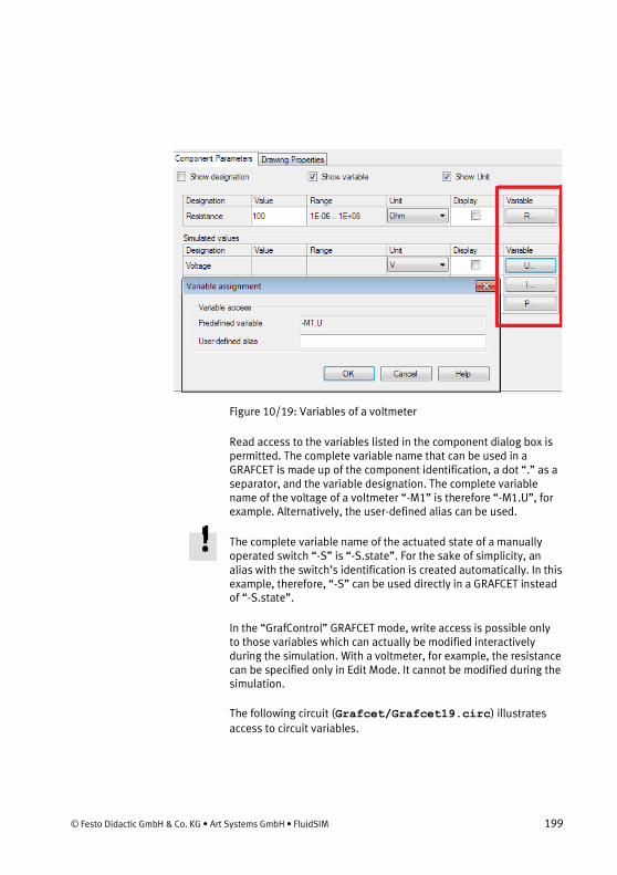
© Festo Didactic GmbH & Co. KG • Art Systems GmbH • FluidSIM 199
Figure 10/19: Variables of a voltmeter
Read access to the variables listed in the component dialog box is permitted. The complete variable name that can be used in a GRAFCET is made up of the component identification, a dot “.” as a separator, and the variable designation. The complete variable name of the voltage of a voltmeter “-M1” is therefore “-M1.U”, for example. Alternatively, the user-defined alias can be used.
The complete variable name of the actuated state of a manually operated switch “-S” is “-S.state”. For the sake of simplicity, an alias with the switch’s identification is created automatically. In this example, therefore, “-S” can be used directly in a GRAFCET instead of “-S.state”.
In the “GrafControl” GRAFCET mode, write access is possible only to those variables which can actually be modified interactively during the simulation. With a voltmeter, for example, the resistance can be specified only in Edit Mode. It cannot be modified during the simulation.
The following circuit (Grafcet/Grafcet19.circ) illustrates
access to circuit variables.

200 © Festo Didactic GmbH & Co. KG • Art Systems GmbH • FluidSIM
Figure 10/20: Access to circuit variables
The “GrafControl” GRAFCET mode is set in the circuit properties, otherwise the action could not act directly on the circuit. The condi-tion checks if the voltage of voltmeter “-M1” is greater than 10 volts. The complete variable name of the voltage is “-M1.U” as described above, and is displayed on the action in the circuit. Once the simulation starts, the voltage can be increased interactively in the function generator. If the voltage exceeds 10 volts, the action becomes active.
Figure 10/21: Access to circuit variables
The variable “-S1” is set, which is an (automatic) alias of “-S1.state”. This sets the state of switch “-S1” to “1” (actuated) and the switch opens.

© Festo Didactic GmbH & Co. KG • Art Systems GmbH • FluidSIM 201
10.5 Monitoring with GRAFCET actions
A GRAFCET can be used to monitor the proper functioning of a fluidic or electrical circuit. The monitoring functionality in FluidSIM allows you to check whether GRAFCET actions executed in a circuit resulted in the desired behavior. This is done by evaluating so-called monitoring conditions in the active actions during the simu-lation. If a monitoring condition is violated, meaning that its value is “0” (FALSE), the corresponding action is marked with a color and the violation of the condition is tolerated for a defined time. Once that time is exceeded, the monitoring is categorized as failed.
The settings for monitoring can be set along with the choice of GRAFCET mode (see "Setting the GRAFCET mode").
Figure 10/22: Settings for GRAFCET monitoring
Here you can define whether you want the monitoring to be carried out during the simulation.
If the monitoring condition of an active action is violated, the action is marked in the color specified.
Once a monitoring condition fails, or in other words, once the tolerance time is exceeded, the corresponding action is marked in the color specified.
Enable monitoring
Monitoring condition false
Action failed

202 © Festo Didactic GmbH & Co. KG • Art Systems GmbH • FluidSIM
If this option is activated, the simulation switches to pause mode when a monitoring condition fails.
If this option is activated, an audio signal is sounded when a moni-toring condition fails.
The following example is designed to illustrate the use of GRAFCET monitoring (Grafcet/Grafcet21_Hyd.circ or Grafcet/Grafcet21_Pneu.circ).
Figure 10/23: Circuit diagram with GRAFCET monitoring
The single action in the GRAFCET activates the solenoid valve directly. This should cause the cylinder piston to advance. A moni-toring condition in the action will be used to check if the cylinder actually did advance. A small positive velocity indicates the advanc-ing of the piston.
To formulate the monitoring condition, open the properties dialog box for the action by double clicking.
Pause simulation on action failed
Play sound on action failed

© Festo Didactic GmbH & Co. KG • Art Systems GmbH • FluidSIM 203
Figure 10/24: Specifying the monitoring condition
The monitoring condition is entered in this field. Circuit variables can be assigned to a unit of measurement by writing the desired unit in square brackets after the variable. This is “1.3.v [m/s]” in the example shown.
In this field you enter the time period after which a violated condi-tion is categorized as failed.
The “Templates” button opens a dialog box where a condition can be compiled interactively.
Monitoring condition
Tolerance time

204 © Festo Didactic GmbH & Co. KG • Art Systems GmbH • FluidSIM
Figure 10/25: Template of a monitoring condition
You can use the two drop-down lists to select a template of a moni-toring condition.
Here you can specify the identification of the component to which
the monitoring condition will refer. You can use the “ Browse... ”
button to select the component from an additional selection dialog box.
Here the variables and units are listed which are used in the select-ed template.
Parameters can be adjusted in some templates. For example, in the template “Cylinder is in interval”, you can specify the limits x1 and x2 of the interval.
Monitoring condition
Component
Variables / Units
Parameter

© Festo Didactic GmbH & Co. KG • Art Systems GmbH • FluidSIM 205
The condition generated from the template is shown as a formula in this field. This formula is transferred into the input field for the monitoring condition.
Start the simulation and observe how the GRAFCET controls the circuit and advances and retracts the cylinder piston.
Figure 10/26: Simulation with GRAFCET monitoring
Now close the one-way flow control valve. The solenoid valve still switches over as a result of the GRAFCET action, but the cylinder cannot advance now. The monitoring condition of the action is now violated and the action is marked in yellow to indicate this viola-tion.
Condition formula

206 © Festo Didactic GmbH & Co. KG • Art Systems GmbH • FluidSIM
Figure 10/27: Simulation with GRAFCET monitoring
After the set tolerance time of one second, the violated condition is categorized as failed, the action is marked red, and the simulation goes into pause mode.

© Festo Didactic GmbH & Co. KG • Art Systems GmbH • FluidSIM 207
Figure 10/28: Simulation with GRAFCET monitoring
10.6 Quick reference for the FluidSIM-relevant GRAFCET concepts
The next sections introduce all GRAFCET concepts that are related to FluidSIM.
10.6.1 Initialization
All the variables in a GRAFCET are preset with the value “0” at the start of the simulation.

208 © Festo Didactic GmbH & Co. KG • Art Systems GmbH • FluidSIM
10.6.2 Sequence rules
— A transition is considered released once all the immediately preceding steps are active. A transition is triggered once it has been released and its condition has the value “1”. A transition with the value “1” is shown in green in FluidSIM, regardless of whether the step linked to it is active or inactive.
— The relevant transition is triggered at the same time and does not take any time.
— Since triggering a transition does not take any time, a step can be activated and deactivated at the same time (even across various intermediate steps). An active step remains active in this situation. A loop of steps is only run through once at one point in time (see example: Grafcet/Grafcet06.ct).
10.6.3 Sequence selection
A step can branch off into various partial sequences. In the GRAFCET specifications, these partial sequences have to be exclu-sive. Since this can generally only be checked during the sequence, this exclusivity is not required in FluidSIM (see example: Grafcet/Grafcet07.ct).
10.6.4 Synchronization
The GRAFCET synchronization component can be used to imple-ment synchronizations (see example: Grafcet/Grafcet08.ct).

© Festo Didactic GmbH & Co. KG • Art Systems GmbH • FluidSIM 209
10.6.5 Transient sequence / unstable step / virtual triggering
As described in Sequence rules, triggering a transition does not take any time. As a consequence of this, multiple consecutive steps can be activated at the same point in time one after the other. This sequence is called transient (continuous).
The intermediate steps in the sequence chain are referred to as unstable. The continuously effective actions connected to them are not displayed in the simulation. The allocations in the stored effec-tive actions are carried out. Triggering the intermediate steps and their associated transitions is called virtual triggering (see example: Grafcet/Grafcet06.ct).
10.6.6 Determining the values of GRAFCET variables
Variables of continuously effective actions (allocations) receive the value “1” if the corresponding action is linked to an active step and any action condition present has the value “1”.
Variables of stored effective actions (assignation) are changed if the corresponding action is linked to an active step and the rele-vant action event occurs (e.g. action on event or on activation).
FluidSIM does not check whether the two types of variable identifi-cation contradict each other for a variable. If this case occurs, the variable value is determined by an internal calculation, which the user cannot predict (see example: Grafcet/Grafcet09.ct).
10.6.7 Checking the entries
FluidSIM checks the validity of entries for conditions and assigna-tions. If this kind of term does not match the specifications, the

210 © Festo Didactic GmbH & Co. KG • Art Systems GmbH • FluidSIM
term in question is displayed in red. The simulation is only released once all the terms are valid.
10.6.8 Admissible characters for steps and variables
Steps and variables cannot contain any spaces. Function names that can be used in a GRAFCET expression are not permitted.
There are no limitations for the descriptions that can be shown for conditions and actions, because these are only displayed and are not used for simulation.
10.6.9 Variable names
There are four different types of variables. All variables can be used in conditions and assignations.
Action variables are available throughout GRAFCET and can be set in actions (see example: Grafcet/Grafcet10.ct).
Step variables are inserted automatically for each step and have the value “1” when and only when the corresponding step is active. Step variables have the form X + “step name”. If, for example, the step name is “12”, then the associated variable is “X12”. Step names are only ever valid within a partial GRAFCET or within the global GRAFCET. This means that the same step name can be used in different partial GRAFCETs. In order to be able to address step variables across partial GRAFCETs in FluidSIM, the step variable has to be preceded by the partial GRAFCET name. Example: Partial GRAFCET “1” contains step “2” and is meant to be addressed in the global GRAFCET. Within the global GRAFCET, the step variable name “G1.X2” has to be used. Within partial GRAFCET “1”, “X2” is enough (see example: Grafcet/Grafcet11.ct). Variables of
macro-steps have the form XM + “step name”, macro inputs have XE + “step name” and macro outputs have XS + “step name” (see example: Grafcet/Grafcet15.ct).
Action Variables
Step Variables

© Festo Didactic GmbH & Co. KG • Art Systems GmbH • FluidSIM 211
Partial GRAFCET variables are automatically inserted for each partial GRAFCET and have the value “1” when and only when at least one step in the corresponding partial GRAFCET is active. Partial GRAFCET variables have the form XG + “partial GRAFCET name”. If, for example, the partial GRAFCET name is “1”, the asso-ciated variable is “XG1” (see example: Grafcet/Grafcet12.ct).
The variables of circuit components can be used in GRAFCETs as input and output variables (see "Access to variables of circuit components").
10.6.10 Functions and formula entry
A range of functions can be used in conditions and assignations. These functions are displayed according to the GRAFCET specifica-tions (e.g. upwards arrow for rising edge). Entering GRAFCET-specific functions is supported by the buttons in the dialogues with the relevant labels:
— “+” (logical OR)
— “*” (logical AND)
— “NOT” (logical NOT)
— “RE” (rising edge)
— “FE” (falling edge)
— “s / / s” (delay)
— “s /” (delay, short form)
— “NOT(s /)” (time limit)
If the functions “NOT”, “RE” or “FE” refer to a term, the term has to be placed in brackets.
Examples:
Partial GRAFCET Variables
Variables of circuit compo-nents

212 © Festo Didactic GmbH & Co. KG • Art Systems GmbH • FluidSIM
NOT a
NOT (a + b)
RE X1
RE (X1 * X2)
The following additional mathematical functions are available:
— abs (absolute amount)
— sign (algebraic sign: +1, 0, -2)
— max (maximum of two numbers)
— min (minimum of two numbers)
— ^ (to the power of, e.g. a^3)
— sqrt (square root)
— exp (to the power of constant “e”)
— log (natural logarithm)
— sin (sine)
— cos (cosine)
10.6.11 Delays / time limits
Delays have the following form (see example: Grafcet/Grafcet03.ct):
“Time in seconds” s / “Boolean term” / “time in seconds”
or
“Time in seconds” s / “Boolean term”

© Festo Didactic GmbH & Co. KG • Art Systems GmbH • FluidSIM 213
Examples:
1 s / X1 / 2s 3s/X3
Time limits have the following form:
NOT (“time in seconds” s / “Boolean term”)
Example: NOT(6s/X28)
In addition to “s” for seconds, the following units of time can also be used.
— d (days)
— h (hours)
— m (minutes)
— s (seconds)
— ms (milliseconds)
Time specifications can also be combined, e.g. “2s500ms” for 2.5 seconds.
10.6.12 Boolean value of an assertion
In GRAFCET, you can use Boolean values to calculate an assertion, for example: a counter “C” should be larger than 6 and step “X1” should be activated. “C” is larger than “6” can be calculated as with a variable. To do this, the assertion has to be set in square brack-ets. So in this example:
[C > 6 ] * X1
If a Boolean assertion is positioned on its own in a condition, then you can omit the square brackets in FluidSIM, for example C > 6 instead of [C > 6]. (See example:Grafcet/Grafcet13.ct)

214 © Festo Didactic GmbH & Co. KG • Art Systems GmbH • FluidSIM
10.6.13 Target information
If you want to interrupt an operative connection from a transition to a step, you can enter the name of the target step in the transition’s properties dialogue (see example: Grafcet/Grafcet14.circ).
10.6.14 Partial GRAFCETs
Partial GRAFCETs can be used to separate a GRAFCET into different hierarchy levels. This function is most often used for enclosing steps and compulsory commands. The name of a partial GRAFCET is always preceded by a “G”.
In order to determine partial GRAFCETs in FluidSIM, the partial GRAFCET frame has to be placed over the relevant GRAFCET part and you have to assign a name in the properties dialogue. The preceding “G” is not part of the name that you have to enter; it is added automatically by FluidSIM and shown at the bottom left of the partial GRAFCET frame. You can alter the size of the partial GRAFCET frame by dragging its edges with the mouse (see exam-ple: Grafcet/Grafcet11.ct). It is important that all the ele-
ments of the partial GRAFCET are located entirely within the rele-vant frame and that there are no “foreign” elements overlapping the frame.
10.6.15 Macro-steps
Macro-steps can be specified using a step’s properties dialogue. The preceding “M” is not a part of the name that you have to enter; it is added automatically by FluidSIM. You can specify macro inputs and macro outputs in the same way. The preceding “E” and “S” in these cases are not part of the name either and are automatically added by FluidSIM (see example: Grafcet/Grafcet15.circ).

© Festo Didactic GmbH & Co. KG • Art Systems GmbH • FluidSIM 215
10.6.16 Compulsory commands
Compulsory commands can be used to control partial GRAFCETs regardless of their normal sequence. There is an entry mask to help you enter these commands in FluidSIM. There are four types of compulsory command. They are shown here using four examples (see example: grafcet/Grafcet16.circ).
Setting a specific situation. This example activates steps 8, 9 and 11 of partial GRAFCET 12.
Freezing a partial GRAFCET. In this example, the current situation for partial GRAFCET 12 is maintained as it is. No further transitions are triggered.
Setting a blank situation. All steps in partial GRAFCET 12 are deac-tivated in this example.
Setting the initial situation. In this example, the steps in partial GRAFCET 12 that are marked as initial steps are activated.
10.6.17 Enclosing step
Enclosing steps can be specified using a step’s properties dialogue. You can either enter the enclosed partial GRAFCETs directly or select them from a list. You have to separate individual partial GRAFCETs with a comma or a blank space.
During simulation, the name of the enclosing step is shown at the top left of the partial GRAFCET frame, as soon as the step is activat-ed (see example: Grafcet/Grafcet17.ct).
You have to set the “Activation link” field in the properties dialogue for steps within the enclosed partial GRAFCET that you wish to activate when the enclosing step is activated.
G12 {8, 9, 11}
G12 {*}
G12
G12 {INIT}

216 © Festo Didactic GmbH & Co. KG • Art Systems GmbH • FluidSIM
10.6.18 Action when a transition is triggered
An action on triggering is a stored effective action which is execut-ed when the transition connected to the action is triggered. The action is usually connected to the transition by a straight line (see example Grafcet/Grafcet20.circ).

Dimension
© Festo Didactic GmbH & Co. KG • Art Systems GmbH • FluidSIM 217
Chapter 1111. Dime nsion
FluidSIM allows both automatic and manual dimensioning.
11.1 Draw dimension
The buttons
Horizontal
Vertical
Align
Angular
Flag
activate the corresponding mode for drawing the dimension ar-rows. Alternatively you can also access the dimensioning functions
in the Draw menu under Dimension .
Horizontal, vertical and diagonal dimensioning is done by defining two points for the distance as well as then clicking to position the dimension text. Angular dimensioning requires the center point to be defined as well as two points for the angle. The fourth click in
turn defines the position of the dimension text. The Flag dimen-
sion function can also be used for general labeling of important points in the circuit. Two points for a line with any pitch and a final click for the text are needed for this.

218 © Festo Didactic GmbH & Co. KG • Art Systems GmbH • FluidSIM
11.2 Settings for the dimension
Figure 11/1: Dimension dialog window
Defines the drawing layer for the dimension.
Activates or deactivates automatic adaptation of the dimension when the dimension length is changed.
If the Automatic Dimensioning option is deactivated you can enter any number that will be displayed as the length dimension. A unit can also be selected. Show Unit defines whether the unit should be displayed.
Defines the number of decimal places.
Determines the factor by which the real length is multiplied for the displayed value. This is necessary if you are creating a drawing with a scale other than 1:1.
Defines the color for the dimension.
Layer
Automatic Dimensioning
Length
Decimals
Factor
Color

© Festo Didactic GmbH & Co. KG • Art Systems GmbH • FluidSIM 219
Defines the line style for the dimension.
Defines the line width for the dimension.
Dimensions, like all other objects in FluidSIM, can be moved, rotat-ed, mirrored and scaled. The display value of the dimension is automatically adapted during scaling if the Automatic Dimension-ing option is activated.
Line Style
Line Width

Component attributes
220 © Festo Didactic GmbH & Co. KG • Art Systems GmbH • FluidSIM
Chapter 1212. Compone nt attributes
The FluidSIM circuit symbols largely correspond to the components in the equipment sets from Festo Didactic GmbH & Co. KG. The parameters of the components are also entered accordingly in FluidSIM. Open the Properties dialog window for a component by
double clicking a symbol or by opening the Edit menu and select-
ing Properties... .

© Festo Didactic GmbH & Co. KG • Art Systems GmbH • FluidSIM 221
12.1 Component attributes in the Properties dialog window
Figure 12/1: Properties dialog window for a component:
The properties of a component are saved in attribute value pairs. The attributes are divided into different groups. The first group contains the general properties:

222 © Festo Didactic GmbH & Co. KG • Art Systems GmbH • FluidSIM
Figure 12/2: Detail from the Properties dialog window for a compo-nent: General properties
Displays the name of the circuit symbol. The symbol name is mapped to appropriate products in the Festo product catalogue. Users cannot edit the symbol name.
Contains a more detailed description or the complete name of the circuit symbol where applicable. Users can edit this. The identifica-tion is shown as text in the circuit drawing if the “Display” option is selected.
The part number uniquely identifies a product within parts lists.
In this selection list you define the drawing layer for the symbol. Depending on the setting for the drawing layer it may not be possi-ble to display or edit the symbol. In order to make the symbol visible or change the settings you have to temporarily activate the
drawing layer on the Drawing Layers... menu item from the View
menu.
Here you can assign an identification that uniquely identifies the component in the circuit diagram. The identification is shown as text in the circuit drawing if the “Display” option is selected.
Note: FluidSIM automatically assigns a unique identification when inserting or copying circuit symbols. An automatically assigned identification text begins with a question mark and can be edited by the user (FluidSIM shows a warning if you are assigning an identifi-cation that already exists).
Deactivate this option if you do not want the symbol to appear in the parts list.
Symbol Name
Description
Part number
Layer
Identification
Display in Parts Lists

© Festo Didactic GmbH & Co. KG • Art Systems GmbH • FluidSIM 223
12.2 User Defined Properties
You can enter your own component attributes in the “User Defined Properties” tab.
Figure 12/3: Detail from the Properties dialog window for a compo-nent: User Defined Properties tab
In order to edit an entry the corresponding row must be selected by clicking on it. Clicking on the table cell to be modified again then enables you to edit the entry in the cell.
A row can be deleted by first clicking the row to highlight it. The
highlighted row can then be deleted using the Del key.
You can add any desired attributes by filling out the empty cells on the last row.

224 © Festo Didactic GmbH & Co. KG • Art Systems GmbH • FluidSIM
12.3 Drawing Properties
You can enter a number of drawing properties that influence how the symbols are displayed in the circuit diagram in the “Drawing Properties” tab.
Figure 12/4: Detail from the Properties dialog window for a compo-nent: Drawing Properties tab
Defines the scaling in the x or y direction. The scaling factor can also be defined with the help of the mouse pointer. This is de-scribed in the “Scale symbols” section.
Defines the angle of rotation in degrees. The angle of rotation can also be defined with the help of the mouse pointer. This is de-scribed in the “Rotate symbols” section.
If this option is activated then another color can be selected for the symbol.
Resets the geometrical settings to the default values: Scaling to 1, rotation to 0 and “Override Color” deactivated.
Scale
Rotation
Override Color
Reset

© Festo Didactic GmbH & Co. KG • Art Systems GmbH • FluidSIM 225
12.4 Main and secondary components
As described under Component attributes in the Properties dialog window, the FluidSIM circuit symbols largely correspond to the components in the Festo product catalogue. These symbols are called main components. However there are also secondary com-ponents, which do not correspond to components in the Festo product catalogue. These secondary components are usually sym-bolic representations of a partial aspect of an associated main component.
All product properties are stored in the main component. The secondary components only have a description and a reference to the associated main component. In electrical engineering in par-ticular, components such as relays are divided into main and sec-ondary components where the coil is the main component and the contacts are the secondary components.
12.5 Linking main and secondary components
Main and secondary components are linked using the symbol for the secondary component. The circuit diagram detail shows a relay comprising a coil as the main component and two contacts as the secondary components. The contacts are to be linked with the coil. This information is evaluated when displaying the contact image.
Figure 12/5: Relay comprising coil with two contacts
The symbol identifications are the defaults used in FluidSIM. The symbols are not linked together yet.

226 © Festo Didactic GmbH & Co. KG • Art Systems GmbH • FluidSIM
→ Open the corresponding properties dialog window by double-clicking a contact.
Figure 12/6: Properties dialog window for a contact
Defines a description for the secondary component. In the case of a contact, this is shown in the terminal diagram.
A compatible main component can be selected from a list. The main component identification can also be entered directly as text.
Opens a dialog that shows all compatible main components as a tree in accordance with the object hierarchy.
If this box is checked then the secondary component is logically linked with the main component. If the main component is then renamed, the link is retained and the identification of the linked secondary component is adapted as appropriate to the main com-ponent identification.
If the secondary component is logically linked with a main compo-nent, a search can be performed for the associated main compo-nent using this button.
If this box is checked then the main component’s identification is shown as the identification for the secondary component.
Description
Main Component
Browse...
Link
Find Target...
Display

© Festo Didactic GmbH & Co. KG • Art Systems GmbH • FluidSIM 227
→ Select “Q1” from the list of compatible main components. Proceed in the same way for the second contact.
Selecting from the list of compatible main components automatical-ly establishes the logical links between the contacts and the coil. The circuit diagram should now look as follows:
Figure 12/7: Relay comprising coil with two contacts
If you now change the coil identification to “Q2”, the logical links mean that the identifications at the contacts will also be automati-cally changed to “Q2”.
Examples of this are relays with the coil as the main component and the contacts as secondary components as well as electromagnetic directional control valves with the pneumatic symbol as the main component and the valve solenoids as secondary components in the electrical part of the circuit diagram.
12.6 Link solenoid valves and solenoid coils
The coils belonging to solenoid valves are usually displayed sepa-rately in the electrical part of a circuit diagram. The link between a solenoid valve and the associated coils is defined at the solenoid valve symbol.
The following circuit diagram shows a solenoid valve and the sym-bols for two separate solenoid coils. No link has been established yet between the solenoid valve and the coils.

228 © Festo Didactic GmbH & Co. KG • Art Systems GmbH • FluidSIM
Figure 12/8: Solenoid valve and two separate coils
There are two ways of establishing a link between a solenoid valve and a coil. The first is using the properties dialog window for the solenoid valve.
→ Open the appropriate properties dialog window by double-clicking the solenoid valve and select the Connector Labels tab.

© Festo Didactic GmbH & Co. KG • Art Systems GmbH • FluidSIM 229
Figure 12/9: Properties dialog window, Connector Labels tab
This tab shows all of the solenoid valve’s connectors. Connectors refer, among other things, to the logical connection options for the solenoid coils. The input fields of the left-hand electric connector are described below. The descriptions apply analogously to the right-hand connector and other types of logical connectors.
The identification for the left-hand solenoid coil can be entered in this list box or selected from a list. When you click in this field the corresponding connector is highlighted in the preview. This helps to locate the connector, particularly when dealing with turned or mirrored symbols.
Electric Connector (Left)

230 © Festo Didactic GmbH & Co. KG • Art Systems GmbH • FluidSIM
Opens a dialog that shows all compatible solenoid coils as a tree in accordance with the object hierarchy.
If this box is checked then the solenoid coil is logically linked with the connector at the solenoid valve. If the solenoid coil is renamed the link is retained and the identifications of the coils at the sole-noid valve are changed to match the coil identifications.
If the connector at the solenoid valve is logically linked with a coil a search can be performed for the associated coil using this button.
If this box is checked the coil’s identification is shown as the identi-fication for the solenoid valve connector.
→ Select “-K1” from the list of compatible solenoid coils.
Figure 12/10: Left connector linked with coil “-K1”
The second way of linking a solenoid valve with a coil is to double-click the solenoid valve’s connector directly. The coil connectors are represented like pneumatic connectors within the solenoid valve by means of small circles.
→ Double-click the right connector of the solenoid valve.
A dialog window whose fields correspond to the entries for a con-nector in the Connector Labels tab of the Properties dialog window.
Browse...
Link
Find Target...
Display

© Festo Didactic GmbH & Co. KG • Art Systems GmbH • FluidSIM 231
Figure 12/11: Connector dialog window
→ Select “-K2” from the list of compatible solenoid coils.
The (electric) connectors of the solenoid valve are now linked with the solenoid coils.
Figure 12/12: Link solenoid valve and solenoid coils
12.7 Attributes of the text components
In FluidSIM text components serve, firstly, to insert comments and labels and, secondly, can be defined by the labels and accessories without displaying a symbol. Open the dialog window Properties of
the text component by double-clicking on a text or via the Proper-
ties... menu item on the Edit menu.

232 © Festo Didactic GmbH & Co. KG • Art Systems GmbH • FluidSIM
Figure 12/13: Properties dialog window for a text component:
A text component possess all of the attributes of a standard com-ponent. The text properties are located on the “Edit Text” tab.

© Festo Didactic GmbH & Co. KG • Art Systems GmbH • FluidSIM 233
Figure 12/14: Detail from the Properties dialog window for a text component: Edit Text tab
Enter your text into the input field on the left-hand side. You can
also enter text with multiple lines. Press the Enter key to create a
line break.
Defines the horizontal or the vertical alignment of the text within the text field.
Defines the text font.
Defines the text color.
Draws a frame around the text field.
If this option is activated a text that identifies a link to an attribute is displayed instead of the text entered. The value of the selected attribute is displayed in the circuit diagram. You can find a detailed description of this function under Link text components with attrib-utes. A predefined placeholder such as the page number can also
be selected using the Predefined variable... button.
Edit Text
Alignment
Font...
Color...
Frame Text
Attribute Link

234 © Festo Didactic GmbH & Co. KG • Art Systems GmbH • FluidSIM
12.8 Link text components with attributes
Text components can also display attributes of other components, values of predefined placeholders, attributes of a circuit or the project. The text component must be linked to the corresponding attribute for this. The linked attribute is defined in the input field of the “Edit Text” tab in the Properties dialog window for the text component. The activated Attribute Link option defines that the text in the text field should not be displayed but rather interpreted as a link.
Example:
Assuming that your project is called “Project1” and possesses the “Supplier” attribute with the value “Festo”. You project contains the “Circuit1” circuit and you would like to display the value of the “Supplier” attribute, in this example namely the value “Festo”, in this circuit diagram.
→ Insert a text component into the circuit drawing by selecting the text element on the drawing elements toolbar and then left-clicking the circuit drawing. The Properties dialog window for the text component then opens.
Note: You can open the dialog window of an existing text compo-
nent by double-clicking it or using the Edit menu and the Prop-
erties... menu item.
→ Activate the Attribute Link option and then click the Browse...
button.
A window opens displaying the hierarchy of all of the available attributes. Please note that only those objects are listed that have an identification assigned by the user. Identifications beginning with a question mark “?” are not listed. These are identifications that have been automatically assigned by FluidSIM. The desired attribute is located under “Attribute Tree” - “Project1” - “Supplier”.

© Festo Didactic GmbH & Co. KG • Art Systems GmbH • FluidSIM 235
Figure 12/15: Browse Attributes dialog window
→ Select “Supplier” and then click the Select button.
The “Project1.Supplier” value is displayed in the input field and “Festo” in the preview. The complete and unique name of the attribute contains all of the hierarchy levels beginning at the pro-ject. The individual layers in the name are separated by a full stop. It is also possible to enter only the attribute name into the input field. In this example: “Supplier”. The hierarchy is then searched from the bottom up for the attribute, beginning with the text com-ponents. If the attribute searched for is not found in that compo-nent then the circuit and then the project are searched for the attribute.
If the attribute is not found then the attribute name is displayed in the circuit diagram in angle brackets. The missing attribute can be created at a later point in time. The link is then created automatical-ly.
The concept of linking text components with attributes is also utilized for labeling von drawing frames.

236 © Festo Didactic GmbH & Co. KG • Art Systems GmbH • FluidSIM
12.9 Text components with specified links
Text components are automatically generated for displayable component attributes and connector labels which are linked to the corresponding attributes. Open the Display Attribute dialog window with which you can adjust how the text is displayed by double-
clicking on the text component or via the Properties... menu item
on the Edit menu.
Figure 12/16: Display Attribute dialog window
Defines the horizontal or the vertical alignment of the text within the text field.
Defines the scaling factor of the text in the x or y direction.
Note: You can also change the text size by selecting another font size in the font type dialog window. You open this dialog window
using the Font... button under Text Attributes.
Defines text’s angle of rotation in degrees.
Defines the text font.
Alignment
Scale
Rotation
Font...
© Festo Didactic GmbH & Co. KG • Art Systems GmbH • FluidSIM 237
Defines the text color.
Draws a frame around the text field.
The target of a linked text is the attribute which the text refers to. This button opens the Properties dialog window of the object which contains this attribute.
12.10 Change the properties of multiple objects simultaneously
If multiple objects are selected, choosing the Properties... menu
item on the Edit menu opens a dialog window with a limited
selection of properties. It only contains those properties which meaningfully relate to all of the selected objects. This enables you to change the font for multiple texts in a single operation, for ex-ample. The more different object types (symbols, connectors, drawing elements, texts, etc.) that are selected, the less common properties are available.
The following tabs are available for the common properties de-pending on the objects highlighted.
12.10.1 Drawing Properties
The dialog elements available within a tab depend on the objects highlighted.
Color...
Frame Text
Find Target...

238 © Festo Didactic GmbH & Co. KG • Art Systems GmbH • FluidSIM
Figure 12/17: Properties dialog window, Drawing Properties tab: several highlighted objects
Defines the font type of the text.
Draws a frame around the text field.
Defines the scaling factor of the text in the x or y direction.
Defines the angle of rotation of the text field in degrees.
Defines the color of the drawing element.
Defines the line style.
Defines the line width.
Defines how the beginning of the line is displayed.
Defines how the end of the line is displayed.
Sets the location of the drawing element to the background. This means that all of the circuit symbols are on top of this. In particular this means that symbols are not covered by filled drawing ele-ments, for example.
Font...
Frame Text
Scale
Rotation
Override Color
Line Style
Line Width
Start Cap
End Cap
Background

© Festo Didactic GmbH & Co. KG • Art Systems GmbH • FluidSIM 239
Sets the location of the drawing element to the foreground. This means that all of the circuit symbols are underneath this. In particu-lar it means that symbols are covered by filled drawing elements, for example.
Reset the settings to the default values.
12.10.2 Main Component
Figure 12/18: Properties dialog window, Drawing Properties tab: several highlighted objects
A compatible main component can be selected from a list. The main component identification can also be entered directly as text.
Opens a dialog that shows all compatible main components as a tree in accordance with the object hierarchy.
If this box is checked then the secondary component is logically linked with the main component. If the main component is then renamed, the link is retained and the identification of the linked secondary component is adapted as appropriate to the main com-ponent identification.
Foreground
Reset
Main Component
Browse...
Link

240 © Festo Didactic GmbH & Co. KG • Art Systems GmbH • FluidSIM
If the secondary component is logically linked with a main compo-nent, a search can be performed for the associated main compo-nent using this button.
Find Target...

Parts list management and analyses
© Festo Didactic GmbH & Co. KG • Art Systems GmbH • FluidSIM 241
Chapter 1313. Parts list manage ment a nd a nalyses
Various analyses can be inserted into a circuit diagram using the
Insert menu item. Alternatively you can also use the button on
the toolbar. The following dialog window opens.
Figure 13/1: List/Table... dialog window
The following analyses can be inserted into the circuit diagram
using this dialog: Parts List , Terminal diagram , Cable Map ,
Cable List , Wiring List and Tube List .
The use of parts lists is described below. The use and function of the other analyses are described in the corresponding chapters.
FluidSIM creates parts lists that are automatically updated in the background while the circuits are being edited.
If a parts list has been added to a circuit diagram as described above it can be used like a symbol. The use of parts lists as a spe-cial page type is described under Display parts list.
You can customize the appearance of the parts list under “ Proper-
ties... ” in the “Appearance” tab. You can see the effects of the
settings straight away in the preview on the right-hand side.

242 © Festo Didactic GmbH & Co. KG • Art Systems GmbH • FluidSIM
If the “Lines per Page” option is selected you can specify the num-ber of lines to be displayed per page. The relevant pages will also be output when the circuit diagram is printed. Buttons for naviga-tion are displayed underneath the page if the list is split across multiple pages.
Figure 13/2: Buttons for navigating through lists
13.1 Display parts list
We recommend setting up one file specifically for the parts list in a project. If you wish to create a circuit drawing without creating a project you can switch the view for this circuit to the parts list view.
Selecting the Parts List menu item from the View menu enables
you to switch from the circuit view to the parts list view. Conversely,
selecting the Circuit Diagram menu item from the View menu
enables you to switch from the parts list view to the circuit view.
A parts list is displayed as a table in the window. You can edit the following options for editing the table:
— Attributes which the user can edit can be entered directly into the corresponding table field.
— Clicking on the column header sorts the rows on the basis of the column clicked. Clicking on the head of the same column again reverses the sorting order.
— You can adjust the column width by dragging the edges of a column header.
— You can change the order of the columns by dragging and dropping a column header in another position.

© Festo Didactic GmbH & Co. KG • Art Systems GmbH • FluidSIM 243
13.2 Find components from the parts on the circuit diagram
FluidSIM enables you to easily find components on the parts list in the circuit diagram and vice versa.

244 © Festo Didactic GmbH & Co. KG • Art Systems GmbH • FluidSIM
Figure 13/3: Finding components from the parts list
You have the following options:
— Clicking on the Find... button on the “Find Target” parts list
column switches to the circuit diagram display and an anima-tion identifies the corresponding components. If the same cir-

© Festo Didactic GmbH & Co. KG • Art Systems GmbH • FluidSIM 245
cuit diagram is already open in another window than the parts list view remains in the active window. The already opened window containing the circuit diagram is moved into the fore-ground and an animation identifies the corresponding circuit diagram symbol.
— When you click a cell in the parts list table an animation identi-fies the corresponding component in all of the opened windows displaying the circuit diagram.
— If you click a column header in the parts list table then both the entire column of the parts list as well as the corresponding components in the associated circuit diagram windows are se-lected.
— If you click a component in a circuit diagram then both this component and the corresponding row in the open parts lists are selected.
13.3 Set parts list properties
In the parts list view clicking on the Properties... button opens
the Parts List Properties dialog window.

246 © Festo Didactic GmbH & Co. KG • Art Systems GmbH • FluidSIM
Figure 13/4: Parts List Properties dialog window: Included Pages tab
Compiles the components with the same attributes.
Lists all of the components individually
Interprets the column contents as numbers, so that “10” appears after “2”, for example.
Only lists the components of the corresponding circuit diagram.
Lists all of the components of the active project.
Lists all of the components of the selected circuit diagrams belong-ing to the active project.
Accumulated Parts List
Single Position Parts List
Sort as Number
Include This Page’s Compo-nents Only
Include All Project Files
Include Selected Files:

© Festo Didactic GmbH & Co. KG • Art Systems GmbH • FluidSIM 247
Figure 13/5: Parts List Properties dialog window: Listed Attributes tab
Lists all of the component attributes within a parts list row.
Only lists selected component attributes within a parts list row.
List All Attributes
List Selected Attributes:

248 © Festo Didactic GmbH & Co. KG • Art Systems GmbH • FluidSIM
Figure 13/6: Parts List Properties dialog window: Print Options tab
In this tab you can adjust the appearance of the parts list printout. In the preview on the right-hand side you can immediately see the effects of the adjustments. You can find information regarding printing a parts list in the “Print circuit diagram and parts list” section.
13.4 Export parts list
You can export the parts list as a text file.,
→ Click the Export... button in the parts list view.

© Festo Didactic GmbH & Co. KG • Art Systems GmbH • FluidSIM 249
A dialog window for selecting a file or entering a new file name appears. After you have entered a file and left the dialog field you can define the following format settings for the export in the Parts List Export dialog window:
Figure 13/7: Parts List Export dialog window
If this option is selected then the names of the attributes appear in the first row of the text file.
Select this option to set the field elements in quotation marks.
The selected separator is used to separate the columns.
13.5 Insert tube list
You can insert a tube list into a circuit diagram.
→ In the Insert menu, select Tube List to insert a tube list into
the circuit diagram. Alternatively you can click the button.
In the selection dialog box that opens, select Tube List .
Column Header
Quotation Marks
Delimiter

250 © Festo Didactic GmbH & Co. KG • Art Systems GmbH • FluidSIM
The mouse pointer changes to a crosshair. Click the position in the circuit diagram where you want to insert the tube list. A dialog window then opens where you can select the associated tubing and customize the appearance.
Figure 13/8: Tube List dialog window, Included Pages tab
Lists only the tubes in the associated circuit.
Lists all tubes in the active project.
Lists all tubes in the selected circuit in the active project.
Include This Page’s Compo-nents Only
Include All Project Files
Include Selected Files:

© Festo Didactic GmbH & Co. KG • Art Systems GmbH • FluidSIM 251
Figure 13/9: Tube List dialog window, Appearance tab
You can customize the appearance of the tube list on the “Appear-ance” tab. You can see the effects of the settings straight away in the preview on the right-hand side.
If the “Lines per Page” option is selected, you can specify the number of lines to be displayed per page. The relevant pages will also be printed in a printout of the circuit diagram. Buttons for navigation are displayed underneath the page if the list is split across multiple pages.
Figure 13/10: Buttons for navigating through lists

Manage projects
252 © Festo Didactic GmbH & Co. KG • Art Systems GmbH • FluidSIM
Chapter 1414. Manage pr ojects
FluidSIM supports the management of projects by compiling differ-ent files under one name in a single project file. This has the fol-lowing benefits: When opening a project all of the associated data is loaded. It is possible to rapidly access files belonging to a project via the project window. Parts lists whose elements are located in different circuit diagram files can be maintained in one project.
14.1 Create new project
→ Select the New... / Project... menu item from the Project
menu and enter a file name for the new project.
Project files possess the prj file suffix. By default they only contain links to files contained in the project. If you wish to pass on a project then you must either pass on all of the associated files along with the project file or activate the “Save Projects as Single File” option.
When creating a new project, a project folder is automatically created to store the project file and all other files belonging to the project. This automatically created project folder has the same name as the project file. If you create the project file in an empty folder this will be used for the project (i.e. another new folder will not be created underneath it). The automatic creation of project directories can be activated and deactivated in the options under Save.
In the project window a project is represented hierarchically as a list. The top element is the project node. Below this are the associ-ated circuit nodes and parts list nodes which can be differentiated from each other via the symbol in front of the name.

© Festo Didactic GmbH & Co. KG • Art Systems GmbH • FluidSIM 253
14.2 Project nodes
Every project possesses one project node as the uppermost ele-ment. All of the project-specific properties are saved with the pro-ject node. Right-clicking on a project node opens a context menu.
You can also find the menu items on the Project menu. Here you
can find the functions for adding and removing files, among other things.
Under the Properties... menu item from the Project menu you
can define properties for the project. Properties that can be speci-fied for both projects and circuits are described under Circuit and project properties.
14.2.1 Project archiving
Project files generally consist of links to the files contained therein. However, where desired FluidSIM can also save the project along with all of the associated files in one single file. Among other things, this makes it easier to pass on the project. Activate the Save Projects as Single File option in the Archiving tab.

254 © Festo Didactic GmbH & Co. KG • Art Systems GmbH • FluidSIM
Figure 14/1: Project dialog window: Archiving tab
If this option is activated all of the files belonging to the project are saved in a single file.
Please note the advice displayed under this option.
14.3 Circuit and parts list nodes
A circuit node is created beneath the project node for every circuit file that belongs to the project. This also applies to parts lists since they are saved as circuits. These are just displayed differently in the window. All of the circuit-specific or parts list-specific properties are saved with the circuit node.
Right-clicking a circuit node opens a context menu containing the following menu items:
Opens the selected circuit or the selected parts list in a window. Double-clicking on the node in the project tree also opens the window.
Save Projects as Single File
Open...
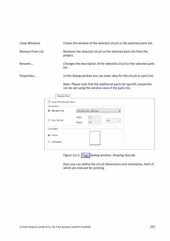
© Festo Didactic GmbH & Co. KG • Art Systems GmbH • FluidSIM 255
Closes the window of the selected circuit or the selected parts list.
Removes the selected circuit or the selected parts list from the project.
Changes the description of the selected circuit or the selected parts list.
In this dialog window you can enter data for the circuit or parts list.
Note: Please note that the additional parts list-specific properties can be set using the window view of the parts list.
Figure 14/2: Page dialog window: Drawing Size tab
Here you can define the circuit dimensions and orientation, both of which are relevant for printing.
Close Windows
Remove From List
Rename...
Properties...

Circuit and project properties
256 © Festo Didactic GmbH & Co. KG • Art Systems GmbH • FluidSIM
Chapter 1515. Circuit and project pr operties
Circuits and projects have a host of common properties. The prop-erties set in the project can be used by circuits in the project. All of the properties that can be specified for both circuits and projects are listed below. The screenshots shown are dialog windows for the circuits.
Figure 15/1: Properties dialog window
The file name field displays the file name of the circuit or project along with the complete path. The file name is carried over to the input field for the “Description” and can be edited there. This entry is displayed in the upper margin of the window as well as beside the circuit or project node.
Here you can specify a page number. The page number can be made up of any character string. The page number can be defined using the “%PageNumber” predefined placeholder. This placehold-er can be used in text components and drawing frames among others.
Properties
Page number

© Festo Didactic GmbH & Co. KG • Art Systems GmbH • FluidSIM 257
Here you can make settings for the drawing frame. This function is described in the section Drawing frame.
15.1 Attributes
Any number of attributes can be created for every circuit or node in a project. The attributes are listed in a table in the “Attributes” tab. New attributes can be entered in the empty cells at the end of the table. The use of attributes is described in the section Attributes of the nodes in a project.
The attributes of a project node are automatically copied to all circuit and parts list nodes (inherited) and are thus available in all of the circuit drawings. This concept is particularly useful for the drawing frames if project attributes are to be displayed in the circuit diagram, for example. You can find further information in the section Link text components with attributes.
Circuit attributes copied from a project cannot be edited initially.
The corresponding row in the Attributes tab of the Page dialog
window is grayed out and the “Inherit From Project” option in the column is activated.
However it is possible to overwrite a copied attribute in a circuit. The option in the “Inherit From Project” column must be deactivat-ed for this. The value of the attribute can then be edited. This function can be used to assign individual page numbers in the drawing frame, for example. If the “Inherit From Project” option is reactivated then the attribute value is copied from the project again.
Drawing Frame

258 © Festo Didactic GmbH & Co. KG • Art Systems GmbH • FluidSIM
Figure 15/2: Attributes tab
This column contains the name of the attribute.
This column contains the value of the attribute.
The buttons in this column allow the following actions: if the attrib-
ute was created in the parent project node then the “ Find Target...
” action is available. Clicking this opens the Project or Circuit dialog window for the project node as the target that contains the corre-sponding attribute. If the attribute was created in the same node
then the “ Delete ” action that allows you to delete the attribute is
available.
If the attribute was created in the same node then this option is deactivated and grayed out. This applies to all of the attributes of the project node since it does not have a parent node. For child nodes the value of the attribute from the project node is copied when this option is activated. After deactivating this option it is possible to locally overwrite the attribute value.
Here you can enter a comment about the attribute.
Attribute
Value
Action
Inherit From Project
Comment

© Festo Didactic GmbH & Co. KG • Art Systems GmbH • FluidSIM 259
15.1.1 Predefined placeholders
FluidSIM provides a host of predefined placeholders. These place-holders can be used in text components and drawing frames among others.
The placeholders begin with a percentage sign. The following predefined placeholders are some of those available:
The page number is specified in the properties dialog window for the circuit diagram.
If analyses are split across several pages, the number of the sub-page is added to the page number with a minus sign. If, for exam-ple, the entered page number is “42-01” and the page displayed is the third page in an analysis then the placeholder “%PageNumber” is replaced by the character string “42-01-03”.
The description for the page is specified in the properties dialog window for the circuit diagram.
Stands for the file name of the page without the file path.
Stands for the file name of the page with the full file path.
Stands for the date and time of the most recent change to the circuit diagram.
Stands for the date of the most recent change to the circuit dia-gram.
Stands for the time of the most recent change to the circuit dia-gram.
%PageNumber
%PageDescription
%PageFileName
%PageFullFilePath
%PageFileDateTime
%PageFileDate
%PageFileTime

260 © Festo Didactic GmbH & Co. KG • Art Systems GmbH • FluidSIM
15.2 Page Dividers
Page dividers can only be defined for pages. Editing of page divid-ers is described under Page dividers.
15.3 Basic Unit Length
The symbols in the FluidSIM symbol libraries are created according to various DIN ISO standards. Instead of specifying absolute units of length, the standards simply use a relative basic unit of length “M”. All of the symbols have been created with reference to this basic unit of length “M”. The actual size of the symbol is not de-fined until the symbol is inserted into a circuit.
Information on how to convert the basic unit of length “M” is stored with the circuit diagram. You can change the set values for a circuit diagram by calling up the properties dialog window for the circuit
diagram using the Page Properties... menu. You will find the
relevant settings in the Basic Unit Length tab.

© Festo Didactic GmbH & Co. KG • Art Systems GmbH • FluidSIM 261
Figure 15/3: Basic Unit Length tab
As soon as the value of “M” is changed, the sizes of the existing symbols are recalculated with respect to the specified basic unit of length. The specification has no effect on elements in the drawing frame.
The Basic Unit Length tab is also in the project settings. The set-tings made in this tab are used as a template for circuit diagrams created from new in the project tree.
15.4 Encryption
Projects and circuit diagrams can be encrypted. The encryption method used is AES-128.

262 © Festo Didactic GmbH & Co. KG • Art Systems GmbH • FluidSIM
Figure 15/4: Encryption tab
This option activates and deactivates encryption. When encryption is activated the password to be used can be entered in the Pass-word input field.
Enable Encryption

© Festo Didactic GmbH & Co. KG • Art Systems GmbH • FluidSIM 263
15.5 Cross Reference Representation
Figure 15/5: Cross Reference Representation tab
This tab is used to define the settings for the cross-reference repre-sentation. You can find further information under Cross-reference representation. If the Inherit From Parent Node option is active then the settings will be copied from the parent project node.
Illustrates the effects of the settings using an example.
Resets the settings to the settings defined in FluidSIM.
Example
Reset

Special functions for electric circuits
264 © Festo Didactic GmbH & Co. KG • Art Systems GmbH • FluidSIM
Chapter 1616. Special functions for electric circuits
16.1 Potentials and conduction lines
The creation of horizontal and vertical potential lines is supported by drawing conduction lines. The end points of the conduction line consist of potentials that also serve as interruptions. In the dialog window for drawing conduction lines you can specify whether the potentials should have an identification.
In this example we want to draw three horizontal potential lines where each line comes from a preceding sheet “1” and is continued on a sheet “3”.
You open a dialog window where you can make the settings shown
using the Insert Conduction Line... menu item or the button
on the toolbar.

© Festo Didactic GmbH & Co. KG • Art Systems GmbH • FluidSIM 265
Figure 16/1: Settings for the potential lines to be created
You can then define the end points of the line with two consecutive mouse clicks.
Figure 16/2: Three horizontal potential lines
The identifications of the potentials can be changed. In this exam-ple we want to rename the potential from L4 to L6.
→ Double-click the left-hand potential L1. Then enter L4 for the identification in the dialog window.
Then following prompt then opens.

266 © Festo Didactic GmbH & Co. KG • Art Systems GmbH • FluidSIM
Figure 16/3:
FluidSIM supports the automatic renaming of the potentials linked with the source potential. If you answer “Yes”, the potential L1 on the right-hand side will also be renamed L4.
→ Rename the potentials L2 and L3 to L5 and L6 in the same way.
→ Then enter the corresponding markers for the predecessors or successors in the properties dialog windows for the potentials. If the corresponding cross-references have the same markers in the respective predecessor and successor pages, the potential lines might look as follows.
Figure 16/4: Three horizontal potential lines with cross-references
16.2 Cables and wiring
Cables and wiring are represented in the circuit diagram by a spe-cial cable symbol. All of the lines defined by the cable symbol are assigned to a cable or to wiring. You can define for the symbol whether it is a cable or wiring.
Wiring only summarizes the defined lines (wires) graphically in the circuit diagram and is assigned the identification “W” by default. Wiring is not listed in analyses such as cable maps and cable lists. Unlike a cable, wiring cannot be assigned to a product. With wiring, product information can only be saved in the lines.

© Festo Didactic GmbH & Co. KG • Art Systems GmbH • FluidSIM 267
If the cable symbol represents a cable then a cable object must be assigned to the symbol. Product properties can be saved in the cable object and are analyzed in cable maps and cable lists, etc. Several cable symbols can reference the same cable object. This is the case if, for example, a cable has to be spread over several pages.
Figure 16/5: Cable symbol
→ Select the Cable menu item from the Insert menu or click
the button to define a cable or wiring.
This activates a mode that allows you to insert a cable symbol by making two consecutive clicks. All of the lines that are defined by the cable symbol are initially assigned to wiring.
If you want to use a cable instead of wiring you can assign a cable object to the symbol using the properties dialog window for the cable symbol.

268 © Festo Didactic GmbH & Co. KG • Art Systems GmbH • FluidSIM
Figure 16/6: Cable Symbol dialog window, Wires tab
Defines the drawing layer for the cable symbol.
Defines whether the cable symbol represents a cable or wiring comprising single wires. Wiring is not listed in cable maps, etc. If Wiring is selected then an identification can be specified that can be displayed with Display Identification.
If Cable is selected then an existing cable object can be assigned to the cable symbol using a drop-down list. A new cable object can be
created using the Create New... button. Clicking Properties...
opens the properties dialog window for the selected cable object.
In order to analyze cable maps the component connections that join a wire must be determined. The connectors are automatically entered in the list box if they can be uniquely assigned. If a unique assignment is not possible, the relevant connector must be select-ed manually via the list box. The identification for the individual
Layer
Cable – Wiring
Wires

© Festo Didactic GmbH & Co. KG • Art Systems GmbH • FluidSIM 269
wires can also be entered. These are saved in the individual lines (wires). The wire identifications are displayed at the cable symbol using the Display button.
The entries in the From and To column are automatically defined as the direction of the wires when creating the cable symbol. Clicking
the Reverse Direction button reverses the directions of all of the
wires.
Clicking this button renumbers all of the wires defined by the cable symbol, starting with the number entered in the list box.
Figure 16/7: Cable Symbol dialog window, Display Attributes tab
In the “Display Attributes” tab you can select the attributes of the associated cable object that are to be displayed at the cable sym-bol.
→ Click the Create New... button to create a new cable symbol.
The following dialog window opens.
Reverse Direction
Renumber From:

270 © Festo Didactic GmbH & Co. KG • Art Systems GmbH • FluidSIM
Figure 16/8: New Cable dialog window
Indicates the page where the cable object will be saved. This is important if various cable symbols on different pages reference the same cable object. The cable object is only saved with one page.
Enter the identification for the cable here.
Enter the number of lines (wires) in the cable here. The number can be higher than the underlying lines if, for example, a concrete cable has unconnected wires. If the associated cable symbols overscore more lines than are defined in the cable object, a warning is output when the page is checked and the corresponding entries are high-lighted in color in the cable lists.
After you specify the identification for the cable and confirm the dialog, the cable object is generated and the cable symbol is as-signed to it.
→ Click the “ Properties... ” button to edit the properties of the
cable object.
Containing Page
Identification
Number of Wires

© Festo Didactic GmbH & Co. KG • Art Systems GmbH • FluidSIM 271
Figure 16/9: Properties dialog window: Cable tab
Defines the number of lines (wires) in the cable. The number can be higher than the lines overscored by the associated cable symbols if, for example, a concrete cable has unconnected wires. If the associ-ated cable symbols overscore more lines than are defined in the cable object, a warning is output when the page is checked and the corresponding entries are highlighted in color in the cable lists.
The associated cable symbols are listed in rows in the table. You
can jump to the associated cable symbol using the “ Find... ”
button.
The User Defined Properties tab in the properties dialog window for the cable symbol lists the cable-specific product properties such as Cable Type and Length. These properties and the entries in the Cable tab are analyzed in the cable map, etc.
Number of Wires

272 © Festo Didactic GmbH & Co. KG • Art Systems GmbH • FluidSIM
16.2.1 Manage cables
All cables within a circuit can be listed and renamed using the
Manage Cables... menu item from the Page menu. You open the
properties dialog window for the relevant cable object using the
Properties... button.
You can also call up the cables of all circuits belonging to the pro-
ject using the Manage Cables... menu item from the Project
menu.
Figure 16/10: Manage Cables... dialog window
Shows which circuit the cable is assigned to. You can edit this assignment within a project.
You can add a new cable object to the project using the Create
New... button. Each cable object must be assigned to a page.
Containing Page

© Festo Didactic GmbH & Co. KG • Art Systems GmbH • FluidSIM 273
Clicking the Create New... button first opens the following dialog
window where you can define the assignment.
Figure 16/11: Browse Pages dialog window
After you click the Select button a dialog window opens where
you can define the name and number of wires for the new cable object. The dialog window is described under Cables and wiring.
16.2.2 Insert cable map
You can insert an associated cable map for a cable into the circuit diagram. You do this by inserting a cable map into a circuit diagram and then assigning a cable to this map.
→ To insert a cable map into the circuit diagram select the Cable
Map menu item from the Insert menu. Alternatively you can

274 © Festo Didactic GmbH & Co. KG • Art Systems GmbH • FluidSIM
click the button. Select Cable Map in the selection dialog
window that opens.
The mouse pointer changes to a crosshair. Click the position in the circuit diagram where you want to insert the cable map. A dialog window then opens where you can assign the relevant cable and customize the appearance.
Figure 16/12: Cable Map dialog window
Defines the relevant cable.
Opens the properties dialog window for the associated cable sym-bol.
Cable
Properties...

© Festo Didactic GmbH & Co. KG • Art Systems GmbH • FluidSIM 275
You can customize the appearance of the cable map in the “Ap-pearance” tab. You can see the effects of the settings straight away in the preview on the right-hand side.
If the “Lines per Page” option is selected you can specify the num-ber of lines to be displayed per page. The relevant pages will also be output when the circuit diagram is printed. Buttons for naviga-tion are displayed underneath the page if the list is split across multiple pages.
Figure 16/13: Buttons for navigating through lists
16.2.3 Insert cable list
You can insert a cable list into a circuit diagram.
→ To insert a cable list into the circuit diagram select the Cable
List menu item from the Insert menu. Alternatively you can
click the button. Select Cable List in the selection dialog
window that opens.
The mouse pointer changes to a crosshair. Click the position in the circuit diagram where you want to insert the cable list. A dialog window then opens where you can select the associated cable and customize the appearance.

276 © Festo Didactic GmbH & Co. KG • Art Systems GmbH • FluidSIM
Figure 16/14: Cable List dialog window, Included Pages tab
Lists only the cables in the associated circuit.
Lists all cables in the active project.
Lists all cables in the selected circuit in the active project.
Include This Page’s Compo-nents Only
Include All Project Files
Include Selected Files:

© Festo Didactic GmbH & Co. KG • Art Systems GmbH • FluidSIM 277
Figure 16/15: Cable List dialog window, Appearance tab
You can customize the appearance of the cable map in the “Ap-pearance” tab. You can see the effects of the settings straight away in the preview on the right-hand side.
If the cable symbols of a cable object overscore more lines than are defined in the cable object, a warning is output when the page is checked and the corresponding entries are highlighted in color in the cable list.
If the “Lines per Page” option is selected you can specify the num-ber of lines to be displayed per page. The relevant pages will also be output when the circuit diagram is printed. Buttons for naviga-tion are displayed underneath the page if the list is split across multiple pages.

278 © Festo Didactic GmbH & Co. KG • Art Systems GmbH • FluidSIM
Figure 16/16: Buttons for navigating through lists
16.2.4 Insert wiring list
You can insert a wiring list into a circuit diagram.
→ To insert a wiring list into the circuit diagram select the Wir-
ing List menu item from the Insert menu. Alternatively you
can click the button. Select Wiring List in the selection di-
alog window that opens.
The mouse pointer changes to a crosshair. Click the position in the circuit diagram where you want to insert the wiring list. A dialog window then opens where you can select the associated wiring and customize the appearance.

© Festo Didactic GmbH & Co. KG • Art Systems GmbH • FluidSIM 279
Figure 16/17: Wiring List dialog window, Included Pages tab
Lists only the wirings in the associated circuit.
Lists all wirings in the active project.
Lists all wirings in the selected circuit in the active project.
Include This Page’s Compo-nents Only
Include All Project Files
Include Selected Files:

280 © Festo Didactic GmbH & Co. KG • Art Systems GmbH • FluidSIM
Figure 16/18: Wiring List dialog window, Appearance tab
You can customize the appearance of the wiring list in the “Appear-ance” tab. You can see the effects of the settings straight away in the preview on the right-hand side.
If the “Lines per Page” option is selected you can specify the num-ber of lines to be displayed per page. The relevant pages will also be output when the circuit diagram is printed. Buttons for naviga-tion are displayed underneath the page if the list is split across multiple pages.

© Festo Didactic GmbH & Co. KG • Art Systems GmbH • FluidSIM 281
Figure 16/19: Buttons for navigating through lists
16.3 Terminals and terminal strips
16.3.1 Set terminals
You can set individual terminals or multiple terminals in one step.
→ Select the Terminal menu item from the Insert menu or
click the button to define an individual electric terminal.
This activates a mode that allows you to insert a terminal by click-ing a free point on the electric line.
Figure 16/20:
As soon as you have set a new terminal in this way the dialog window containing the settings for this terminal appears. You can use this dialog window to assign the terminal to a terminal strip. This assignment can also be made or changed later.

282 © Festo Didactic GmbH & Co. KG • Art Systems GmbH • FluidSIM
Figure 16/21: Terminal dialog window
Contains the description of the terminal or the terminal designa-tion.
If this box is checked then the description entered will be displayed beside the terminal.
Defines the drawing layer for the line.
Defines the position of the terminal within the associated terminal strip. An entry is only possible once the terminal has been assigned to a terminal strip.
Changes the direction of the terminal. The direction is indicated in the circuit by an arrow that shows which connector is inside the control cabinet and which is outside. The tip of the arrow points into the control cabinet.
If this box is checked then the direction arrow is displayed at the terminal.
Defines the terminal strip containing the terminal in question. The list contains the terminal strips already created. You call up the properties dialog window for the selected terminal strip using
Description
Display
Layer
Pos.
Internal # External
Show Direction
Terminal Strip

© Festo Didactic GmbH & Co. KG • Art Systems GmbH • FluidSIM 283
Properties... . You can also create a new terminal strip using
Create New... .
If this box is checked then the identification for the associated terminal strip is displayed beside the terminal.
16.3.2 Set multiple terminals
As well as the option of setting individual terminals, FluidSIM also offers a mode that allows you to set multiple terminals one after the other. You can keep inserting terminals by simply clicking on the electric lines until you leave the mode again.
→ To insert multiple terminals select the Multiple Terminals...
menu item from the Insert menu or click the button.
Figure 16/22:
The operation begins with a dialog window where you can make some settings for the new terminals. Above all you need to first select an existing terminal strip or create a new one. If a suitable
Display Identification

284 © Festo Didactic GmbH & Co. KG • Art Systems GmbH • FluidSIM
terminal strip does not already exist then a prompt to create a new one will automatically appear.
Figure 16/23: Define Multiple Terminals dialog window
Defines how the new terminals are to be numbered. The Enumerate Manually option allows you to specify a start number from which the numbering continues. Otherwise a free terminal from the se-lected terminal strip is automatically used. The start number “2” was specified in the example shown.
If this box is checked then the description entered will be displayed beside the terminal.
Defines the direction of the new terminals. The direction is indicat-ed in the circuit by an arrow that shows which connector is inside the control cabinet and which is outside. The tip of the arrow points into the control cabinet. The direction can also be changed later using the properties dialog window for the individual terminals.
Defines the drawing layer for the line.
Defines the terminal strip containing the terminals in question. The list contains the terminal strips already created. You call up the properties dialog window for the selected terminal strip using
Description
Display
Direction
Layer
Terminal Strip

© Festo Didactic GmbH & Co. KG • Art Systems GmbH • FluidSIM 285
Properties... . You can also create a new terminal strip using
Create New... .
If this box is checked then the identification for the associated terminal strip is displayed beside the new terminals.
16.3.3 Create terminal strips
FluidSIM does not treat terminal strips as visible objects within the circuit pages which explains why they cannot be interactively selected using the mouse in order to highlight them, delete them or change their properties. Terminal strips can either be managed via
the associated terminals or using the Manage Terminal Strips...
menu item under Page or Project .
A terminal strip is always part of a specific circuit. To define a new terminal strip you must therefore define a circuit file in addition to the description and number of terminals.
Figure 16/24: New Terminal Strip dialog window
All properties can also be changed later at any time. You open the properties dialog window for a terminal strip via any terminal in
that terminal strip using the Properties... button.
Display Identification

286 © Festo Didactic GmbH & Co. KG • Art Systems GmbH • FluidSIM
Figure 16/25: Terminal Strip dialog window
If the target of a terminal inside the control cabinet is unique due to the wiring, FluidSIM automatically enters the identification for the connected component. Otherwise the list contains the identifica-tions of all objects that can be reached from the terminal. The target search can be controlled by selecting a junction symbol as a T distributor.
The targets of the terminals outside the control cabinet are listed here. As with the internal targets, unique links are automatically entered.
Jumps to the associated terminal in the circuit diagram.
16.3.4 Manage terminal strips
All terminal strips within a circuit can be listed and renamed using
the Manage Terminal Strips... menu item from the Page menu.
You open the properties dialog window for the relevant terminal
strip using the Properties... button.
External Target
Internal Target
Find...

© Festo Didactic GmbH & Co. KG • Art Systems GmbH • FluidSIM 287
You can also call up the cables of all terminal strips belonging to
the project using the Manage Terminal Strips... menu item from
the Project menu.
Figure 16/26: Manage Terminal Strips... dialog window
Shows which circuit the terminal strip is assigned to. You can edit this assignment within a project.
You can add a new terminal strip to the project using the Create
New... button. Each terminal strip must be assigned to a page.
Clicking the Create New... button first opens the following dialog
window where you can define the assignment.
Containing Page

288 © Festo Didactic GmbH & Co. KG • Art Systems GmbH • FluidSIM
Figure 16/27: Browse Pages dialog window
After you click the Select button a dialog window opens where
you can define the properties of the new terminal strip. The dialog window is described under Create terminal strips.
16.4 Terminal diagram
You can insert an associated terminal diagram for a terminal strip into the circuit diagram. You do this by inserting a terminal diagram into a circuit diagram and then assigning a terminal strip to this diagram.
→ Select the Terminal diagram menu item from the Insert
menu or click the button to insert a terminal diagram into the circuit diagram. Alternatively you can click the button.
Select Terminal diagram in the selection dialog window that
opens.

© Festo Didactic GmbH & Co. KG • Art Systems GmbH • FluidSIM 289
The mouse pointer changes to a crosshair. Click the position in the circuit diagram where you want to insert the terminal diagram. A dialog window then opens where you can assign the relevant terminal strip and customize the appearance.
Figure 16/28: Terminal diagram - Properties dialog window
Defines the associated terminal strip.
Opens the properties dialog window for the associated terminal strip.
You can customize the appearance of the terminal diagram in the “Print Options” tab. You can see the effects of the settings straight away in the preview on the right-hand side.
If the “Lines per Page” option is selected you can specify the num-ber of lines to be displayed per page. The relevant pages will also
Terminal Strip
Properties...

290 © Festo Didactic GmbH & Co. KG • Art Systems GmbH • FluidSIM
be output when the circuit diagram is printed. Buttons for naviga-tion are displayed underneath the page if the list is split across multiple pages.
The entries in the “Description”, “Identification” and “Connector” columns are taken from the object properties of the associated targets.
16.4.1 Set links
You can set so-called links in a terminal strip. These links are drawn in the circuit diagram as regular electric lines and marked as links. The representation of the T distributors can be customized using their properties dialog window.
The following example shows a circuit diagram with a terminal strip X1 with 10 terminals and the associated terminal diagram. A link plug is to be placed at level “1” between terminals “7” and “8” and at level “2” between terminals “8” and “9”, and a wire link is to be placed between terminals “9” and “10”.

© Festo Didactic GmbH & Co. KG • Art Systems GmbH • FluidSIM 291
Figure 16/29:
→ Double-click the electric line between terminals “7” and “8”.

292 © Festo Didactic GmbH & Co. KG • Art Systems GmbH • FluidSIM
Figure 16/30:
The properties dialog window for the electric line opens. The op-tions for setting the links are in the top right:
Figure 16/31: Detail of the Line (electric) dialog window
Defines that this line is to be treated as a link.
Defines that the link is a link plug.
Specifies the level if a link plug was selected.
Defines that the link is a wire link.
→ Set “Link”, “Link Plug” and “Level 3”.
FluidSIM tracks the line across one distributor point at most. This means that the specified link will find the contacts “7” and “8”. This link will be represented in the terminal diagram as follows.
Link
Link Plug
Level
Wire Link

© Festo Didactic GmbH & Co. KG • Art Systems GmbH • FluidSIM 293
Figure 16/32:
→ Proceed in the same way to set a link plug between “8” and “9” at level “2” and a wire link between “9” and “10”.
The terminal diagram then has the following appearance.

294 © Festo Didactic GmbH & Co. KG • Art Systems GmbH • FluidSIM
Figure 16/33:
16.5 Contact images
The contact images can be displayed within a circuit diagram be-neath relay coils and similar symbols. The contact images list all the contacts of the associated relay coil and show which current paths these contacts are in. The division of the page or circuit diagram can be defined using the page dividers.
→ To do this select the Display Contact Images menu item from
the View menu.
The contact images of the current circuit diagram are shown or hidden.
Contact images can be highlighted, moved and aligned like other symbols.

© Festo Didactic GmbH & Co. KG • Art Systems GmbH • FluidSIM 295
Figure 16/34:
You can have all of the contacts in a contact image displayed in a list and customize the appearance by double-clicking the contact
image or highlighting the contact image and selecting the Proper-
ties... menu item from the Edit menu.

296 © Festo Didactic GmbH & Co. KG • Art Systems GmbH • FluidSIM
Figure 16/35: Contact Image dialog window
You can customize the representation of the contact image in the “Print Options” tab.
The “Contacts” tab lists all of the associated contacts. You can jump to the corresponding contact in the circuit diagram using the
Jump to Target button.

Circuit input and output
© Festo Didactic GmbH & Co. KG • Art Systems GmbH • FluidSIM 297
Chapter 1717. Circuit input and output
17.1 Print circuit diagram and parts list
FluidSIM circuits and parts lists can be printed by opening the Print dialog window via the Print... menu item on the File menu.
In FluidSIM a parts list is the representation of a circuit as a table. If you wish to print an individual parts list then the corresponding circuit must be shown in the parts list display.

298 © Festo Didactic GmbH & Co. KG • Art Systems GmbH • FluidSIM
Figure 17/1: Print dialog window:
Select the desired output device from the list of the available print-ers.
This button enables you to open the dialog window for setting the printer options.
Activate this option if you wish to write the print data to a file.
When you work in a project you can select which circuits and parts lists are to be printed.
Printer
Properties...
Print to File
Print Project Files
Copies

© Festo Didactic GmbH & Co. KG • Art Systems GmbH • FluidSIM 299
Select the number of copies. If the printout consists of multiple pages you can cause FluidSIM to print a correspondingly sorted sequence.
You can increase or decrease the output size by entering a scaling factor. If the dimensions of the area to be printed are larger than the printable area on the paper then the printout is spread across multiple pages (tiled). You can see the page divisions in the print preview.
Note: Please note that it may not always be possible to precisely comply with the page margins. Therefore you should plan a certain amount of leeway for the page margin.
Here you can specify additional margins in order to manually cus-tomize the print area.
You can select which page the print preview displays.
17.2 Import DXF file
Files saved in the DXF format can be imported and retain most of their element attributes. If several special points were taken into account when creating the drawing using a CAD program then FluidSIM can easily expand the symbol library.
17.3 Export circuit
The FluidSIM circuits can be saved as a file with a variety of differ-ent formats. The BMP, JPG, GIF, WMF, PNG, DXF, TIF and PDF for-
mats are available. Once you have selected the Export... menu
item from the File menu a dialog window opens where you can
define the different settings for the export. The settings depend on the format selected.
Scale
Page
Margins

300 © Festo Didactic GmbH & Co. KG • Art Systems GmbH • FluidSIM
Figure 17/2: Export Page dialog window
You are then prompted to select a file name or enter a new one.
Select a suitable resolution for the image file.
Please note that a high resolution generates extremely large files which mean the export may take longer. However you can cancel the image export at any time.

Options
© Festo Didactic GmbH & Co. KG • Art Systems GmbH • FluidSIM 301
Chapter 1818. Options
You can access the various program settings in the Options dialog
window via the Options... menu item on the Tools menu.
18.1 General
Figure 18/1: Options dialog window: General tab
In order to simplify connection of connectors FluidSIM draws a small circle around the connectors on the circuit symbols. Deacti-vate the Display Snap Radius option in order to disable the display of the snap-in circles.
Activate the Frame fluidic identification option if you want fluidic identifications to be framed automatically. This simplifies the depiction of circuits in accordance with standards.
Activate the Frame Electric Identification option if you want electri-cal identifications to be framed automatically. This simplifies the depiction of circuits in accordance with standards.
View
Frame fluidic identification
Frame Electric Identification

302 © Festo Didactic GmbH & Co. KG • Art Systems GmbH • FluidSIM
Here you can set how you can zoom in or out of the page view with the mouse.
When this option is activated, make switches that are actuated in their initial position are displayed as break switches. Conversely, break switches that are actuated in their initial position are dis-played as make switches.
Here you can set the grid width and the style. To display the grid,
select the Show Grid menu item on the View menu.
As well as absolute values such as “mm” you can also specify the relative basic unit length “M”.
18.2 Save
Figure 18/2: Options dialog window: Save tab
FluidSIM normally compresses the saved files in order to save space on the disk. If you deactivate the option the files are saved as XML files without compression. You can find further information in the Circuit files section.
Zoom
Display initially actuated closer as opener
Grid
Compress Files

© Festo Didactic GmbH & Co. KG • Art Systems GmbH • FluidSIM 303
The “Create Backup Files” option causes the previous versions of saved files are created with the bak file suffix. This enables you to
restore previous versions.
Project files generally consist of links to the files contained therein. However, where desired FluidSIM can also save the project along with all of the associated circuit files in one single file. This serves to simplify passing on or archiving the project, among other things. You can set whether a project saves links or all of the associated files using the Project dialog window – Properties of the project. This option defines the default setting for new projects.
A folder with the project name where all project files are stored is automatically generated when a new project is created if this op-tion is active.
18.3 Folder Locations
Figure 18/3: Options dialog window: Folder Locations tab
This is the default path for opening and saving circuits.
This is the default path for opening and saving projects.
This is the default path for opening and saving libraries.
Create Backup Files
Save New Projects as Single File
Create Folder For New Pro-jects
Page Files
Project Files
Library Files

304 © Festo Didactic GmbH & Co. KG • Art Systems GmbH • FluidSIM
This is the default path for opening and saving drawing frames.
18.4 Language
Figure 18/4: Options dialog window: Language tab
Defines the languages for the program interface including dialog windows and messages.
18.5 Dimension
This tab is used to define the default settings for the dimensions. You can find further information under Dimension.
Drawing Frames
Program

© Festo Didactic GmbH & Co. KG • Art Systems GmbH • FluidSIM 305
Figure 18/5: Options dialog window: Dimension tab
All of the settings are only applied to newly generated dimensions. They have no effect on existing dimensions in the circuit.
Defines the drawing layer where the newly generated dimensions are placed.
Activates and deactivates automatic dimensioning. If this option is activated then the displayed dimension value is automatically adapted if the dimension is scaled.
Defines the unit to be used for the dimension.
Defines whether the unit should be displayed.
Defines the number of decimal places.
Determines the factor by which the real length is multiplied for the displayed value. This is necessary if you are creating a drawing with a scale other than 1:1.
Layer
Automatic Dimensioning
Unit
Show Unit
Decimals
Scale Factor

306 © Festo Didactic GmbH & Co. KG • Art Systems GmbH • FluidSIM
18.6 Cross Reference Representation
Figure 18/6: Options dialog window: Cross Reference Representa-tion tab
This tab is used to define the default settings for the cross-reference representation. You can find further information under Cross-reference representation.
The settings are only applied to newly generated projects or cir-cuits. They have no effect on existing objects.
Illustrates the effects of the settings using an example.
Resets the settings to the settings defined in FluidSIM.
Example
Reset

© Festo Didactic GmbH & Co. KG • Art Systems GmbH • FluidSIM 307
18.7 Connector Links
Figure 18/7: Options dialog window: Connector Links tab
Only connectors of the same type can be connected if this option is active. For example a line from an electric connector to a pneumatic connector cannot be created in this case.
FluidSIM supports the automatic connection of connectors. The following settings define which connections should be automatical-ly created.
Pneumatic connectors that are on one horizontal line will be auto-matically connected when a symbol is inserted or moved.
Pneumatic connectors that are on one vertical line will be automati-cally connected when a symbol is inserted or moved.
Electric connectors that are on one horizontal line will be automati-cally connected when a symbol is inserted or moved.
Electric connectors that are on one vertical line will be automatical-ly connected when a symbol is inserted or moved.
Allow connections between same connector types only
Pneumatic – Horizontal
Pneumatic – Vertical
Electric – Horizontal
Electric – Vertical

308 © Festo Didactic GmbH & Co. KG • Art Systems GmbH • FluidSIM
18.8 Warnings
Figure 18/8: Options dialog window: Warnings tab
Different types of warnings that FluidSIM should or should not deliver can be activated and deactivated here. These warnings include “Duplicated identification labels” and “Superimposed objects”.
All of the circuits will be checked during editing if this option is active. Only the criteria that would lead to the warnings specified under “Show Warnings” are checked. Objects that caused an error are highlighted in red in the circuit. If this option is not active then
the check must be initiated manually using the Page – Check
Drawing menu.
Show Warnings
Enable Background Check

© Festo Didactic GmbH & Co. KG • Art Systems GmbH • FluidSIM 309
18.9 Automatic Updates
Figure 18/9: Options dialog window: Automatic Updates tab
FluidSIM can search on the Internet for a new version when the program starts. You can activate or deactivate the automatic search here.
As soon as there is an Internet connection you can use this button to initiate the search for a new FluidSIM version.
Check for updates at startup
Check for updates now...

310 © Festo Didactic GmbH & Co. KG • Art Systems GmbH • FluidSIM
18.10 Simulation
Figure 18/10: Options dialog window: Simulation tab
Normally FluidSIM calculates all data required for the simulation automatically, without bothering the user with mathematical de-tails. However, in some cases it can be useful to specify a certain increment, for example, in order to achieve a more accurate display of high frequencies in electronics. For instance, if you want a reso-lution in the microsecond range, enter an increment of at least 0.000001 (or in scientific notation 1e-6).
Note that simulation in real time is no longer possible if the incre-ments are very small.
You can use this factor to set the ratio of time in which the simulat-ed processes should take place. A value of “1:1” means simulation in real time; “1:10” would mean that the simulation takes place in slow motion, in this case ten times slower than in reality. A ratio of “1:0.1”, for example, would mean the simulation is accelerated ten times. Specifications for real time or accelerated processes can only be fulfilled if the computer has sufficient processing power.
Display interval
Slow-motion factor

© Festo Didactic GmbH & Co. KG • Art Systems GmbH • FluidSIM 311
During the simulation, the pneumatic, hydraulic, electrical, and digital lines will be colored according to their state. You can cus-tomize the colors for each state.
In digital technology, it is useful if unused inputs on AND, NAND, and NOT components are automatically set to Hi. Otherwise, for example, an AND gate with three inputs would not function as expected if only two inputs were wired. So that the circuit does not become cluttered with unnecessary permanently Hi level signals, FluidSIM can set unused inputs on the relevant components to Hi automatically. If you do not want this automatic function, you can switch it off. To prevent misunderstandings regarding unused digital inputs, FluidSIM displays a corresponding message at the start of every simulation. If you do not want this message to ap-pear, you can switch it off.
Note that these values are only used if no others are defined in the page or project properties.
Line colors
Digital Technique (Compati-bility with Siemens LOGO!Soft)

312 © Festo Didactic GmbH & Co. KG • Art Systems GmbH • FluidSIM
18.11 GRAFCET
Figure 18/11: Options dialog window: GRAFCET tab
Here you can set the mode that FluidSIM will apply when handling GRAFCETs during the simulation.
In this mode, GRAFCETs are treated as drawings only. They are not incorporated into the simulation. See also Drawing only (GrafEdit).
This mode uses GRAFCETs for visual presentation of the simulation. The defined actions, however, have no effect on the simulation. In particular, they do not in any way control the fluidic or electrical components. See also Observation (GrafView).
In this mode, the GRAFCET has access to all the circuit variables that can be set from outside. This allows it to switch valves over or to adjust throttle valves See also Control (GrafControl).
When this option is switched on, the GRAFCET monitors the proper functioning of a fluidic or electrical circuit. For this purpose, you can formulate conditions in the actions which will be checked during the simulation. For more details, see Monitoring with GRAFCET actions.
GRAFCET mode
GrafEdit (GRAFCET is not simulated)
GrafView (GRAFCET visual-izes simulation)
GrafControl (GRAFCET con-trols simulation)
Enable monitoring

© Festo Didactic GmbH & Co. KG • Art Systems GmbH • FluidSIM 313
Note that these settings are only used if no others are defined in the page or project properties.
18.12 DDE Connection
Figure 18/12: Options dialog window: DDE Connection tab
Here you can set the default values for the DDE interface.
Note that the server name is a global setting of the specific system environment and is not saved with the circuit data. If you want to use the DDE interface in other environments, ensure that the DDE options are adapted accordingly. In particular, ensure that the DDE connection is activated, because it is switched off by default for security reasons.
18.13 Environment parameters
Figure 18/13: Options dialog window: Environment parameters tab
Here you can set the default values for the environment parame-ters.

314 © Festo Didactic GmbH & Co. KG • Art Systems GmbH • FluidSIM
Note that these values are only used if no others are defined in the page or project properties.
18.14 Fluid properties
Figure 18/14: Options dialog window: Fluid properties tab
This list contains typical oils and other fluids. If you select a prede-fined fluid, the listed values will be set accordingly.
Note that these values are only used if no others are defined in the page or project properties.
18.15 Sound
When you click the “Sound” tab in the Options... menu, a dialog
box appears with parameters for the sound settings:
Fluid type

© Festo Didactic GmbH & Co. KG • Art Systems GmbH • FluidSIM 315
Figure 18/15: Options dialog window: Sound tab
You can activate/deactivate an audible signal for the components Switch/Contact, Relay, Valve, Cylinder, and Buzzer.
Enable sound

316 © Festo Didactic GmbH & Co. KG • Art Systems GmbH • FluidSIM
18.16 Text Sizes
Figure 18/16: Options dialog window: Text Sizes tab
This tab defines the font sizes to be used for objects newly inserted into the circuit diagram.
This group lists the font sizes used for identifications and cross-references, etc.
This group lists the font sizes used for analyses and tables.
Label/Attribute
List/Table

Menu overview
© Festo Didactic GmbH & Co. KG • Art Systems GmbH • FluidSIM 317
Chapter 1919. Menu overview
19.1 File
New
New / File...
Opens a new window for creating a new circuit drawing.
New / Project...
Opens the dialog window for creating a new project.
Open
Open / File...
Opens a new window for selecting an existing circuit drawing.
Open / Project...
Opens the dialog window for selecting an existing project.
Add
Adds files, etc. to the active project.

318 © Festo Didactic GmbH & Co. KG • Art Systems GmbH • FluidSIM
Add / New Page...
Creates a new circuit file and adds it to the active project.
Add / New Parts List...
Creates a new parts list and adds it to the active project.
Add / Existing Files...
Opens the dialog window for selecting existing files to be added to the active project.
Close
Closes the active window or project, etc.
Close / File...
Closes the active window.
Close / Project...
Closes the active project.
Save File
Saves the circuit diagram in the active window to disk.
Save File As...
Saves the circuit diagram in the active window to disk under a new name.
Save Project
Saves the active project.

© Festo Didactic GmbH & Co. KG • Art Systems GmbH • FluidSIM 319
Save Project As...
Saves the active project under a new name on the data storage medium. Files that are within the project folder are duplicated while references to external files are left. With external file references you must therefore consider that changes to these files affect all pro-jects containing them.
Save as Component Library...
Saves the active project as a library. As a result a new library sym-bol is generated for every circuit. The new library bears the name of the project with the lib file suffix.
DXF Import...
Opens the dialog window for selecting a saved DXF file. The select-ed file is subsequently converted into a FluidSIM circuit diagram. The original file remains unchanged.
Export...
Exports the circuit diagram in the active window to the data storage medium as a BMP, JPG, GIF, WMF, PNG, DXF or TIF file.
Page Setup...
Sets up the printer properties for a page to be printed.
Print Preview
Opens a print preview as a page view.
Print...
Opens the FluidSIM Print dialog window to set the print options for the active circuit.

320 © Festo Didactic GmbH & Co. KG • Art Systems GmbH • FluidSIM
Recent Files
A file can be selected for opening from a list of the recently opened files.
Recent Projects
The most recently opened projects can be selected for opening from a list.
Exit
Ends FluidSIM.
19.2 Edit
Undo
Undoes the last editing action for the active circuit.
Redo
Takes back the last undo-action for the active circuit.
Cut
Deletes the selected objects and adds them to the clipboard.
Copy
Copies the selected objects to the clipboard
Paste
Pastes the objects from the clipboard into the active circuit.

© Festo Didactic GmbH & Co. KG • Art Systems GmbH • FluidSIM 321
Delete
Deletes the selected objects from the active circuit.
Select All
Selects all of the objects from the active circuit.
Group
Groups the selected objects.
Create Macro Object
Creates a macro object out of the selected objects.
Create Cross-reference
Creates a cross-reference.
Ungroup/Break Off
Ungroups the selected groups or macro objects.
Enable Scale
Activates or deactivates the “enable scaling” mode which enables the scaling of symbols with the help of the mouse pointer.
Enable Rotate
Activates or deactivates the “enable rotate” mode which enables the rotation of symbols with the help of the mouse pointer.
Edit Poly Line
Activates or deactivates the “Edit Polyline” mode that allows you to edit a polyline.

322 © Festo Didactic GmbH & Co. KG • Art Systems GmbH • FluidSIM
Align
Aligns the selected objects with each other.
Rotate
Rotates the selected objects by 90, 180 or 270 degrees anti-clockwise. Grouped objects are rotated around the center point of the group rectangle.
Mirror
Mirrors the selected objects horizontally or vertically. Grouped objects are mirrored along the axis of the group rectangle.
Properties...
Opens the Properties dialog window for the selected circuit sym-bols in order to enter the component properties.
The Connector dialog window is opened for the selected compo-nent connector enabling you to enter the connector properties.
When a line segment is highlighted a dialog window opens ena-bling you to enter the line properties.
If multiple objects are selected then a dialog window with a limited selection of properties appears. It only contains those properties which affect all of the selected objects.
19.3 Insert
Find Symbol Description...
Opens the search dialog for selecting a symbol via its appearance or its description.

© Festo Didactic GmbH & Co. KG • Art Systems GmbH • FluidSIM 323
Conduction Line...
Opens a dialog window that defines the settings for one or more conduction lines that are to be inserted in the circuit diagram after the dialog window is confirmed.
Interruption/Potential...
Adds an interruption or an electric potential to the circuit diagram.
Parts List
Inserts a parts list into the circuit diagram.
Terminal
Inserts a terminal into the circuit diagram.
Multiple Terminals...
Inserts multiple terminals into the circuit diagram.
Terminal diagram
Inserts a terminal diagram into the circuit diagram.
Cable
Inserts a cable into the circuit diagram.
Cable Map
Inserts a cable map into the circuit diagram.
Cable List
Inserts a cable list into the circuit diagram.

324 © Festo Didactic GmbH & Co. KG • Art Systems GmbH • FluidSIM
Wiring List
Inserts a wiring list into the circuit diagram.
Tube List
Inserts a tube list into the circuit diagram.
19.4 Draw
This menu contains functions for freely drawing graphical elements such as lines, rectangles, circles, etc as well as for inserting texts and images.
Line
Draws a line by defining two defined end points.
Poly Line
Draws a polyline by defining the vertices with successive mouse clicks. The drawing operation can be cancelled by pressing the
Esc key or clicking the right mouse button. The last vertex must
be set with a double-click.
Rectangle
Draws a rectangle by defining two diagonally opposite corner points.
Circle
Draws a circle by defining a middle point and a radius.

© Festo Didactic GmbH & Co. KG • Art Systems GmbH • FluidSIM 325
Ellipse
Draws an ellipse by defining a middle point and a radii on parallel axes.
Text
Inserts a text at the mouse position.
Picture
Inserts an image at the mouse position.
Dimension
Inserts a dimension symbol.
19.5 Page
Check Drawing
Checks the active circuit drawing for drawing errors.
Paper Size...
Opens a dialog window enabling you to set the paper size.
Manage Terminal Strips...
Opens a dialog window enabling you to manage the terminal strips in the circuit.
Manage Cables...
Opens a dialog window enabling you to manage the cable objects in the circuit.

326 © Festo Didactic GmbH & Co. KG • Art Systems GmbH • FluidSIM
Properties...
Opens an dialog window enabling you to set the circuit properties.
19.6 Execute
Stop
Switches the currently active circuit into Edit Mode.
Start
Starts the simulation (animation) in the currently active circuit.
Pause
Pauses the simulation in the currently active circuit without exiting Simulation Mode.
If Pause is clicked when in Edit Mode, the currently active circuit
switches to Simulation Mode without starting the simulation. This allows you to set component states before starting the simulation.
Reset
Resets a circuit to its initial state when a simulation is running or paused. The simulation is then restarted immediately.
Single Step
Stops the simulation after a small step. In other words, the simula-tion is started for a short period of time before being switched back into pause mode ( ). You can switch into single step mode directly from an actively running simulation.

© Festo Didactic GmbH & Co. KG • Art Systems GmbH • FluidSIM 327
Simulate until State Change
Starts the simulation and runs it until a state change happens; the simulation is then paused ( ). A state change happens when a cylinder piston moves against a stop, a valve switches over, or a relay or a switch is actuated. You can switch into state change mode directly from an actively running simulation.
Next topic
Switches to the next topic in a presentation.
19.7 Didactics
Component description
Opens the help page for the selected component. It contains the DIN symbol for the component, a short description of the compo-nent function, the terminal designations, and a list of any adjusta-ble parameters, with value ranges for those parameters.
Tutorial ’Simulating with FluidSIM'
Opens the tutorial “Simulating with FluidSIM”.
Component Library
Opens the reference containing information about the components in the component library.
Didactics Material
Opens an overview of the didactics material. If you copied the film files onto your hard disk during installation, the list of training film chapters will also appear here.

328 © Festo Didactic GmbH & Co. KG • Art Systems GmbH • FluidSIM
Circuits for exercises (TP)...
Opens a dialog box with exercise circuits for the Festo technology packages.
Presentation...
Opens a dialog box that you can use to retrieve and create presen-tations. Presentations allow you to combine separate training topics into a cohesive teaching unit.
Extended Presentation...
Opens a dialog box that you can use to retrieve existing presenta-tions in Microsoft PowerPoint format. The presentation files of the extended presentations are located in the ppx subfolder of your
FluidSIM installation. You can create your own PowerPoint presen-tations and add them by saving them in “ppt” or “pps” format to the ppx folder.
19.8 Project
Add Current Window
Adds the active window to the file list of the open project.
Remove Current Window
Removes the active window from the file list of the open project.
Manage Terminal Strips...
Opens a dialog window enabling you to manage the terminal strips in the project.

© Festo Didactic GmbH & Co. KG • Art Systems GmbH • FluidSIM 329
Manage Cables...
Opens a dialog window enabling you to manage the cable objects in the project.
Manage Cross References...
Opens a dialog window enabling you to manage the cross-references in the project.
Properties...
Opens the dialog window for entering the project properties.
19.9 View
Circuit Diagram
Switches from the parts list view to the circuit diagram view.
Parts List
Switches to the parts list view.
Library
Shows or hides the libraries window.
Project
Shows or hides the window for managing the project files.
Standard Size
Displays the circuit diagram in its original size.

330 © Festo Didactic GmbH & Co. KG • Art Systems GmbH • FluidSIM
Previous View
Displays the previous view of the circuit diagram. Repeatedly activating this function switches back and forth between the views previously used.
Fit to Window
Set the zoom level to fit the entire circuit diagram into the window.
View Detail
Defines the new view by drawing a rectangle while holding down the left mouse button.
Zoom In
Zooms the view of the circuit diagram in by one step. Three steps correspond approximately to doubling the zoom factor.
Zoom Out
Zooms the view of the circuit diagram out by one step. Three steps correspond approximately to halving the zoom factor.
Show Page Borders
Shows or hides the page borders in the form of a red rectangle. This rectangle displays the borders of the paper format defined on the
Paper Size... menu. Using the print preview you can decide
whether and how the drawing is distributed among multiple sheets when printing.
Show Grid
Shows a background grid in the active circuit window. The grid
settings can be made in the General tab under the Options...
menu item from the Tools menu.
© Festo Didactic GmbH & Co. KG • Art Systems GmbH • FluidSIM 331
Show Rulers
Shows or hides the rulers in the active circuit window.
Show Page Dividers
Shows or hides the page dividers in columns and rows. Cross-references can refer to the column and row containing a symbol. The position and number of the columns and rows can be interac-tively defined via the page dividers shown.
Quantity Values...
Opens a dialog box for display of quantity values. Here you can define how each quantity value listed (“velocity”, “pressure”,
“current”, ...) is to be displayed (“ None ”, “ Individual ”, “ All ”).
Show Flow Direction
When this option is active, small arrows are placed on pneumatic and hydraulic lines as a visual indication of the flow direction.
Show Flow Animation
When this option is active, the flow in pneumatic and hydraulic lines is made visible by animating the lines like conveyor belts.
GRAFCET...
Opens a dialog box for display of GRAFCET descriptions. Here you can set whether to display the descriptions or the formulas of GRAFCET elements. Note that this option may overwrite the specific settings of individual elements.
Display Current Path Numbering
When this option is active, the current path designations are shown in the electrical circuits. The division of the page or circuit diagram can be defined using the page dividers.

332 © Festo Didactic GmbH & Co. KG • Art Systems GmbH • FluidSIM
Show Connector Descriptions
Shows or hides the connector descriptions. The Display option can be selected in the properties dialog window for the connectors. This
option is only evaluated if “ Individual ” was selected.
Show Connector Descriptions / All
Shows all connector descriptions regardless of the settings at the connectors.
Show Connector Descriptions / Individual
Shows only the connector descriptions for those connectors with the Display option activated.
Show Connector Descriptions / None
Hides all connector descriptions regardless of the settings at the connectors.
Show Terminal Directions
Shows or hides the direction arrows at the terminals. The tip of the arrow points into the control cabinet here.
Show Terminal Directions / All
Shows all arrows regardless of the settings at the terminals.
Show Terminal Directions / Individual
Shows only the arrows for those terminals with the Show Direction option activated.
Show Terminal Directions / None
Hides all arrows regardless of the settings at the terminals.

© Festo Didactic GmbH & Co. KG • Art Systems GmbH • FluidSIM 333
Display Contact Images
Shows or hides the contact images.
Drawing Layers...
Opens a Drawing Layers dialog window enabling you to set the properties of the drawing layers.
19.10 Library
Add New Library...
Creates a new library.
Add Existing Library...
Opens the dialog window enabling you to select a saved library file with the lib file suffix. The library saved in the file is added to the
library window.
Add Existing Symbol Folder...
Opens the dialog window for selecting an existing folder. The entire contents of the selected folder, including all of the circuit symbols and sub-folders contained therein are displayed as a library.
Close Current Library
Removes the active library from the list in the library window. The library file is not deleted by this action and can be opened again
using the Library menu and the Add Existing Library... menu
item.

334 © Festo Didactic GmbH & Co. KG • Art Systems GmbH • FluidSIM
Rename Active Library...
Opens a dialog window for entering the name of the library. This function is only available to libraries which the user has created. For write-protected libraries the folder name is shown in the tab.
Sort Current Library Alphabetically
Sorts the contents of the active library alphabetically. This function is only available to libraries which the user has created. Write-protected libraries are automatically sorted and cannot be resorted by the user.
19.11 Tools
Options...
Opens the dialog window with program settings, file paths and language options.
Expert Mode
Switches Expert Mode on and off. Expert Mode provides advanced options for editing and simulation.
Restore Defaults...
Resets the program settings to the default values. This enables you to undo unintentional settings made.
Note: Use this function if you feel that FluidSIM is behaving unex-pectedly or files and windows have suddenly disappeared.

© Festo Didactic GmbH & Co. KG • Art Systems GmbH • FluidSIM 335
19.12 Window
New Window
Opens a window with an additional view of the active window.
Navigation Pane
Opens an overview window with a scaled-down view of the entire circuit diagram. The currently visible area of the active window appears as a white area. The non-visible area of the drawing is shaded grey. By drawing a rectangle in the overview window with the mouse pointer you can define the section of the circuit diagram displayed in the active window. Simply left-clicking on the overview window moves the visible area while retaining the zoom level.
Cascade
Arranges the windows so that they overlap.
Tile Horizontally
Arranges the windows into horizontal tiles.
Tile Vertically
Arranges the windows next to each other.
Close All
Closes all open windows.

336 © Festo Didactic GmbH & Co. KG • Art Systems GmbH • FluidSIM
19.13 Help
Contents
Displays the contents of the FluidSIM help pages.
Index
Displays the index of the FluidSIM help pages.
Search
Displays the search dialog for the FluidSIM help pages.
Register as user...
Opens a dialog box via which you can register if you would like assistance and information about FluidSIM.
Check for updates...
As soon as there is an Internet connection you can use this menu item to initiate the search for a new FluidSIM version.
About...
Displays the FluidSIM program information.

Functional diagram
© Festo Didactic GmbH & Co. KG • Art Systems GmbH • FluidSIM 337
Chapter 2020. Functional diagra m
You can find the function diagram in the standard FluidSIM library.
You can apply the functions from the Edit menu to the function
diagram. Double-click the function diagram or open the Functional
diagram using the Properties... menu item on the Edit menu.
The buttons in the upper toolbar of the editor are for editing a function diagram. The following six buttons determine the editing mode:
Edit Mode
Draw diagram curves
Insert signal elements
Insert text boxes
Draw signal lines and insert signal connections
Insert additional signal lines
The selected mode is highlighted in white or displayed as a pressed
button. shows that signal lines can be drawn in the diagram area by clicking, for example.
If you hover the mouse pointer over a button for a short period of time then a short description is displayed.

338 © Festo Didactic GmbH & Co. KG • Art Systems GmbH • FluidSIM
Figure 20/1:
20.1 Edit Mode
This mode serves to adjust the objects in the function diagram. Elements in the diagram can be moved. Changing the size of text boxes is only possible in this mode.
Movement and dragging operations can be cancelled using the
Esc key.
If the mouse pointer is moved outside the window area while the left mouse button is held down the view automatically scrolls.
Double-clicking on a diagram element (diagram row, text box, signaling element, etc.) opens a dialog window in which you can make the desired adjustments.
20.1.1 Set diagram properties
Clicking on the button opens a dialog window in which you can set the diagram properties.
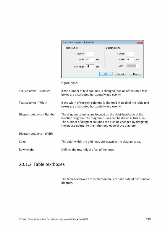
© Festo Didactic GmbH & Co. KG • Art Systems GmbH • FluidSIM 339
Figure 20/2:
If the number of text columns is changed than all of the table text boxes are distributed horizontally and evenly.
If the width of the text columns is changed than all of the table text boxes are distributed horizontally and evenly.
The diagram columns are located on the right-hand side of the function diagram. The diagram curves can be drawn in this area. The number of diagram columns can also be changed by dragging the mouse pointer to the right-hand edge of the diagram.
The color which the grid lines are drawn in the diagram area.
Defines the row height of all of the rows.
20.1.2 Table textboxes
The table textboxes are located on the left-hand side of the function diagram.
Text columns – Number
Text columns – Width
Diagram columns – Number
Diagram columns – Width
Color
Row height

340 © Festo Didactic GmbH & Co. KG • Art Systems GmbH • FluidSIM
Figure 20/3:
Double-clicking on a table textbox opens the corresponding dialog window.
Figure 20/4:
The font size of the text to be shown.
A selection from sixteen standard colors for the text to be dis-played.
The width of the selected table column can be changed by dragging the mouse pointer.
The height of the selected table column can be changed by drag-ging the mouse pointer.
The following alignment options are available: “Left” “Center” and “Right”.
The following alignment options are available: “Top”, “Center” and “Bottom”
Font size
Color
Width
Height
Horizontal adjustment
Vertical adjustment

© Festo Didactic GmbH & Co. KG • Art Systems GmbH • FluidSIM 341
If a text within a textbox should resemble a table then set a tab stop between the text parts. The text is displayed in the textbox in ac-cordance with the number of tab stops and the specified horizontal
and vertical alignment. To enter tab stops hold down the Ctrl
key.
Examples:
1.
2.
Insert text boxes
Alignment within a table cell

342 © Festo Didactic GmbH & Co. KG • Art Systems GmbH • FluidSIM
20.1.3 Adjust the presentation of the diagrams
The area in which curves can be drawn is located on the right-hand side of a diagram row.
Figure 20/5:
Double-clocking on this area opens a corresponding window in which you can define the appearance of the drawing area. Please ensure that no diagram element, such as a signaling element, for example, is underneath the mouse pointer.
Figure 20/6:
The entry defines the number of states and thus the number of horizontal lines in the diagram row.
States – Number

© Festo Didactic GmbH & Co. KG • Art Systems GmbH • FluidSIM 343
Horizontal lines are drawn through the base state with a thin pencil.
The start column defines which column the numbering should begin with.
The start number defines which number the numbering should begin with.
The number specified how many steps need to be numbered.
Defines the step width between two numbers.
If this field is selected then an equals sign and the start number are always displayed after the last number.
If this field is selected then two arrows are displayed.
If this field is selected then the background grid is displayed.
If this field is selected then a textbox is shown which can serve as a label. This textbox belongs to the selected row and cannot be moved to another row.
If this field is selected then an additional textbox is shown which can serve as a label. This textbox belongs to the selected row and cannot be moved to another row.
Sets the color of the diagram lines.
20.2 Draw diagram curve
In this mode diagram curves can be drawn. Supporting points can only be inserted on the grid. A supporting point is drawn at every left-click.
1. 2. 3. 4.
States – Base state
Numbering – Start column
Numbering – Start number
Numbering – Number
Numbering – Step width
Numbering – Loop
Representation – Display arrows
Representation – Display grid
Representation – Display text 1
Representation – Display text 2
Representation – Line color

344 © Festo Didactic GmbH & Co. KG • Art Systems GmbH • FluidSIM
If you hold down the left mouse button then supporting points can be moved as in the selection mode.
Selected supporting points are shown in grey. Use the Del key to
delete a selected symbol.
20.3 Insert signal elements
In this mode signaling elements can be inserted by left-clicking.
1. 2.
If you hold down the left mouse button then signaling elements can be moved as in the selection mode.
Selected signaling elements are shown in grey. Use the Del key
to delete a selected signaling element.
Double-clicking on a signaling element in the selection mode opens a dialog window in which you can modify how the signaling element is shown.

© Festo Didactic GmbH & Co. KG • Art Systems GmbH • FluidSIM 345
Figure 20/7:
If this field is selected then a text is shown which can serve as a label for the signaling element.
The signaling element is displayed in this color.
20.4 Insert text boxes
In this mode textboxes can be inserted by left-clicking.
1. 2. 3.
Selected textboxes are shown in grey. Use the Del key to delete
a selected textbox.
Signal type
Display description
Color

346 © Festo Didactic GmbH & Co. KG • Art Systems GmbH • FluidSIM
In “Edit Mode” the size and position of a textbox can be changed using the mouse pointer.
Adjust size:
1. 2. 3.
Move textbox:
1. 2. 3.
Double-clicking on a textbox in the selection mode opens a dialog window in which you can modify how the textbox is shown.
Figure 20/8:
The font size of the text to be shown. Font size

© Festo Didactic GmbH & Co. KG • Art Systems GmbH • FluidSIM 347
A selection from sixteen standard colors for the text to be dis-played.
If this field is selected then a frame is drawn around the textbox.
The width of the textbox.
The height of the textbox.
The following alignment options are available: “Left”, “Center” and “Right”.
The following alignment options are available: “Top”, “Center” and “Bottom”
Table textboxes
20.5 Draw signal lines and insert signal connections
In this mode signal lines can be drawn freely or automatically laid from signaling elements.
20.5.1 Free-draw signal lines
An additional supporting point is set with every left-click. The process ends when you click the current line while holding down
the Ctrl key, press the Esc key or switch the editing mode. Use
the Del key to delete a selected signal line. If only a supporting
point is selected then only this is removed from the line.
In “Edit Mode” the supporting points belonging to the signal lines
can be moved. If the Shift is held down while setting or moving
Color
Frame
Width
Height
Horizontal adjustment
Vertical adjustment

348 © Festo Didactic GmbH & Co. KG • Art Systems GmbH • FluidSIM
supporting points then the supporting point is vertically or horizon-tally aligned.
In the selection mode double-clicking can change the way the line is displayed.
Figure 20/9:
A framed label on the line and a label next to the framed label is shown. The framed label can be moved freely along the line. The additional label can be moved freely.
An arrow is displayed at the beginning of the line. The arrow can be moved freely along the line.
An arrow is displayed at the end of the line. The arrow can be moved freely along the line.
Line color
If you click a finished signal line to activate the “Freely move signal
lines” mode then a signal logic is inserted. This logic point (snap point) can then be freely moved along the line 1.
2. 3. + 4. .
In the selection mode you can change how the signal logic is dis-played by double-clicking on it.
Display description
Start with arrow
End with arrow
Color

© Festo Didactic GmbH & Co. KG • Art Systems GmbH • FluidSIM 349
Figure 20/10:
20.5.2 Drawing signal lines from signals
In the “Freely draw signal lines” signal lines can be drawn from signals. Left-click a signal and hold down the mouse button. Drag the mouse pointer to a position which you have selected as the end point of a signal line. The signal line will be drawn once you release the mouse button.
1. 2. 3.
20.5.3 Draw signal lines from diagram support points
In the “Freely draw signal lines” mode signal lines can be drawn from curve support points. Left-click a supporting point and hold down the mouse button. Drag the mouse pointer to a second supporting point. The signal line will be drawn once you have the

350 © Festo Didactic GmbH & Co. KG • Art Systems GmbH • FluidSIM
mouse pointer over the second supporting point and release the mouse button.
1. 2. 3.
20.6 Insert additional signal lines
In the “Insert additional signal lines” mode additional support-ing points can be inserted into existing signal lines.
1. 2. 3.
20.7 Insert row
Clicking on the “Insert row” button inserts a new diagram row above the current selection. If no cell is market then a new row is attached to the end of the diagram.
20.8 Delete row
Clicking on the “Delete row” button deletes a selected diagram row. If nothing is selected then the function is not available.

© Festo Didactic GmbH & Co. KG • Art Systems GmbH • FluidSIM 351
20.9 Additional editing functions
20.9.1 Zoom
Using the button the view is reset to the standard zoom level.
Using the button increases the zoom level.
Using the button decreases the zoom level.
20.9.2 Undo editing steps
Using the button you can undo the last 50 editing steps.
Using the button you can redo the previously undone editing steps.

The Component Library
352 © Festo Didactic GmbH & Co. KG • Art Systems GmbH • FluidSIM
Chapter 2121. The Component Library
In FluidSIM each component in the component library is assigned a physical model. Using these models, FluidSIM first creates a global behavior model of the circuit which is then processed during simu-lation.
This chapter provides for a short description of the components in FluidSIM ’s component library. If the component has adjustable parameters, their value ranges are given. A number in brackets after the value range indicates the default setting for the parame-ter.
21.1 Hydraulic Components
21.1.1 Service Components
Pump unit
The pump unit supplies a constant volumetric flow. The operating pressure is limited by the internal pressure relief valve. The pump unit has two tank connections.
Adjustable parameters Opening pressure: 0 ... 40 MPa (6) Revolution: 0 ... 5000 1/min (1450) Displacement: 0.1 ... 5000 cm3 (1.6) Internal leakage: 0 ... 10 l/(min.bar) (0.002)

© Festo Didactic GmbH & Co. KG • Art Systems GmbH • FluidSIM 353
Pump unit (simplified)
Simplified representation of the detailed pump unit. The compo-nent does not have tank connections in the circuit diagram.
Adjustable parameters Delivery rate: 0 ... 500 l/min (2) Maximum pressure: 0 ... 40 MPa (6) Internal leakage: 0 ... 10 l/(min.bar) (0)
Fixed displacement pump
The fixed displacement pump delivers a constant volumetric flow rate dependent upon the revolutions and the displacement volume.
Adjustable parameters Revolution: 0 ... 5000 1/min (1320) Displacement: 0.1 ... 10000 cm3 (1.6) Maximum pressure: 0.1 ... 40 MPa (6) Internal leakage: 0 ... 10 l/(min.bar) (0)
Variable displacement pump
The revolutions of the variable displacement pump can be changed under operating conditions. The pump delivers a variable volumet-ric flow rate dependent upon the variable revolutions and the displacement volume.
Adjustable parameters Revolution: 0 ... 5000 1/min (1320) Displacement: 0.1 ... 10000 cm3 (1.6) Flow rate ratio: 0 ... 100 % (100) Maximum pressure: 0.01 ... 40 MPa (6) Internal leakage: 0 ... 10 l/(min.bar) (0)

354 © Festo Didactic GmbH & Co. KG • Art Systems GmbH • FluidSIM
Proportional pump
The revolutions of the variable displacement pump can be changed proportionally from zero to maximum through a voltage signal between 0 V and 10 V and the assistance of a proportional-amplifier. The pump delivers a variable volumetric flow rate de-pendent upon the variable revolutions and the displacement vol-ume.
Adjustable parameters Mode of control: Displacement control, Speed control (Displace-ment control) Displacement: 0.1 ... 5000 cm3 (1.6) Revolution (min): 0 ... 5000 1/min (0) Revolution (max): 0 ... 5000 1/min (1320) Flow rate ratio (min): 0 ... 1 (0) Flow rate ratio (max): 0 ... 1 (1) Maximum pressure: 0.01 ... 40 MPa (6) Internal leakage: 0 ... 10 l/(min.bar) (0)
Power pack with LS variable and fixed displacement pump combi-nation on a single motor
The hydraulic power pack is suitable for all basic tests of mobile hydraulics. The two pumps are both driven by one electric motor. The vane pump with adjustable delivery rate has a load sensing pump controller. The fixed displacement pump is secured by a pressure relief valve. The pump/motor unit sits on the tank. The return into the tank passes through a return flow filter. The ventila-tion of the tank is also filtered. The oil level can be seen on the sight glass with temperature display. The motor is switched on and off from a control console and is safeguarded against overloading.
Adjustable parameters Revolution: 0 ... 5000 1/min (910) Displacement (Variable displacement pump): 0 ... 10000 cm3 (5.6044) Opening pressure (Variable displacement pump): 0 ... 40 MPa (5)

© Festo Didactic GmbH & Co. KG • Art Systems GmbH • FluidSIM 355
Spring preload: 0.1 ... 10 MPa (1.17) Displacement (Fixed displacement pump): 0 ... 10000 cm3 (4.5055) Opening pressure (Fixed displacement pump): 0 ... 40 MPa (5)
Steering unit (Orbitrol)
The steering unit is used to steer vehicles that are equipped with hydrostatic steering.
The steering unit consists of a proportional rotary valve, a pump control valve and a dosing pump. The rotary valve is opened pro-portional to torque (steering force) and direction of rotation. The control edges of the proportional valve are arranged radially at several levels on the rotary piston and the inside of the rotary valve housing. A spring package assures a spring centered, closed mid-position.
Adjustable parameters External torque: -10 ... 10 N.m (0) Displacement: 0 ... 10000 cm3 (32) Hydraulic resistance: 1e-6 ... 1000 bar.min2/l2 (0.1)
Steering unit (Orbitrol)
The steering unit is used to steer vehicles that are equipped with hydrostatic steering.
The steering unit consists of a proportional rotary valve, a pump control valve and a dosing pump. The rotary valve is opened pro-portional to torque (steering force) and direction of rotation. The control edges of the proportional valve are arranged radially at several levels on the rotary piston and the inside of the rotary valve housing. A spring package assures a spring centered, closed mid-position.
Adjustable parameters

356 © Festo Didactic GmbH & Co. KG • Art Systems GmbH • FluidSIM
External torque: -10 ... 10 N.m (0) Displacement: 0 ... 10000 cm3 (32) Hydraulic resistance: 1e-6 ... 1000 bar.min2/l2 (0.1)
Tank
The tank is integrated into the pump unit and has a pressure of 0 MPa. It can be inserted into the circuit diagram as an independent component.
Hose with quick-action coupling
The hose is available in 3 lengths: 600 mm, 1500 mm, and 3000 mm. The pressure loss in a hose is taken into account by specifying a hydraulic resistance. In FluidSIM no pressure loss is simulated with simple connections between two components.
Adjustable parameters Hydraulic resistance: 1e-6 ... 1000 bar.min2/l2 (0.1)
Hydraulic reservoir
The reservoir enables the performance of a hydraulic system to be optimized. For example, it can be utilized as an energy reservoir and for the absorbance of pressure surges or flow fluctuations. Reservoirs are capable of absorbing a defined volume of fluid under pressure and releasing it again with minimal losses. The construc-tion consists essentially of a pressure resistant container, generally a gas charge of nitrogen and a separator e.g. a piston, a membrane or a bubble elastomer. Hydraulic fluid only starts to flow into the reservoir when the fluid pressure is greater than the gas-preload pressure.
Adjustable parameters

© Festo Didactic GmbH & Co. KG • Art Systems GmbH • FluidSIM 357
Volume: 0.01 ... 100 l (0.32) Pre-load pressure: 0 ... 40 MPa (1) Polytropic exponent: 0.5 ... 3 (1.4)
Hydraulic reservoir
The reservoir enables the performance of a hydraulic system to be optimized. For example, it can be utilized as an energy reservoir and for the absorbance of pressure surges or flow fluctuations. Reservoirs are capable of absorbing a defined volume of fluid under pressure and releasing it again with minimal losses. The construc-tion consists essentially of a pressure resistant container, generally a gas charge of nitrogen and a separator e.g. a piston, a membrane or a bubble elastomer. Hydraulic fluid only starts to flow into the reservoir when the fluid pressure is greater than the gas-preload pressure.
Adjustable parameters Volume: 0.01 ... 100 l (0.32) Pre-load pressure: 0 ... 40 MPa (1) Polytropic exponent: 0.5 ... 3 (1.4)
Diaphragm accumulator with shutoff block
Stores the pressure and is equipped with a pressure relief valve to prevent overpressure.
Adjustable parameters Pre-load pressure: 0 ... 40 MPa (1) Volume: 0.01 ... 100 l (0.32) Opening pressure: 0 ... 35 MPa (8)

358 © Festo Didactic GmbH & Co. KG • Art Systems GmbH • FluidSIM
Filter
The filter limits the contamination of the fluid respecting a certain tolerance value in order to reduce the risk of damage at the com-ponents.
Adjustable parameters Hydraulic resistance: 1e-6 ... 1000 bar.min2/l2 (0.001)
Cooler
An unacceptable fall in the hydraulic fluid’s viscosity can be avoid-ed through the use of a cooler.
Adjustable parameters Hydraulic resistance: 1e-6 ... 1000 bar.min2/l2 (0.001)
Heater
The hydraulic fluid’s optimal viscosity can be reached quickly through the use of a heater.
Adjustable parameters Hydraulic resistance: 1e-6 ... 1000 bar.min2/l2 (0.001)
Connection (hydraulic)
A hydraulic connection is a place where a hydraulic line can be attached to. To simplify the line drawing process, a connection appears as a small circle in Edit Mode. Hydraulic connections can be shut by means of a blind plug. An open hydraulic connection

© Festo Didactic GmbH & Co. KG • Art Systems GmbH • FluidSIM 359
may result in leaking oil; FluidSIM thus pops up a warning mes-sage, if some hydraulic connection was left open. Note that at each hydraulic connection values for the flow and pressure can be dis-played.
Line (hydraulic)
A hydraulic line is used to connect two hydraulic connectors. These may be either a simple hydraulic connection or a T-junction.A hydraulic line is normally treated as an ideal connection, with no pressure drop being included in the simulation. A frictional loss can be entered via the “Physical model” options. If you select “Simple resistance”, only the “Hydraulic resistance” parameter will be included in the simulation. If you select “Pipe model (Hagen-Poiseuille/Blasius)”, a complex empirical calculation is carried out using a model based on Hagen-Poiseuille for laminar flows and a model based on Blasius for turbulent flows, utilizing the Reynolds number and the wall surface roughness.
Adjustable parameters Physical model: Ideal connection,Simple resistance, Pipe model (Hagen-Poiseuille/Blasius) (Ideal connection) Length: 0.01 ... 1000 m (1) Inner diameter: 0.1 ... 1000 mm (6.3) Surface roughness: 0 ... 100 mm (0) Hydraulic resistance: 1e-6 ... 1000 bar.min2/l2 (0.08)
T-junction (hydraulic)
A T-junction joins up to four hydraulic lines, thus having a single pressure potential. Note that T-junctions are introduced automati-cally by FluidSIM when dropping the line drawing cursor onto another line in Edit Mode.

360 © Festo Didactic GmbH & Co. KG • Art Systems GmbH • FluidSIM
21.1.2 Configurable Way Valves
Configurable 2/n way valve
The configurable 2/n way valve is a way valve with two connec-tions, where both its body elements and its operation modes are user-definable.
Additionally, the hydraulic connections can be closed with blind plug.
Adjustable parameters Desired position: 0 ... 4 (0) Hydraulic resistance: 1e-6 ... 1000 bar.min2/l2 (0.164) Positioning time: 1e-4 ... 10 s (0.02) Reset time: 1e-4 ... 10 s (0.03) Minimum voltage: 0.1 ... 300 V (20) Electrically left at U_min: 0.01 ... 100 N (70) Electrically right at U_min: 0.01 ... 100 N (70) Mechanically left: 0.01 ... 100 N (100) Mechanically right: 0.01 ... 100 N (100) Physical spring force: 0.01 ... 100 N (30) Minimum force: 0.01 ... 100 N (20) Min. pilot control force: 0.01 ... 100 N (15) Left: 0.01 ... 100 cm2 (1) Right: 0.01 ... 100 cm2 (1) Pilot control left: 0.01 ... 100 cm2 (1) Pilot control right: 0.01 ... 100 cm2 (1)
Configurable 3/n way valve
The configurable 3/n way valve is a way valve with three connec-tions, where both its body elements and its operation modes are user-definable.

© Festo Didactic GmbH & Co. KG • Art Systems GmbH • FluidSIM 361
Additionally, the hydraulic connections can be closed with blind plugs.
Adjustable parameters Desired position: 0 ... 4 (0) Hydraulic resistance: 1e-6 ... 1000 bar.min2/l2 (0.164) Positioning time: 1e-4 ... 10 s (0.02) Reset time: 1e-4 ... 10 s (0.03) Minimum voltage: 0.1 ... 300 V (20) Electrically left at U_min: 0.01 ... 100 N (70) Electrically right at U_min: 0.01 ... 100 N (70) Mechanically left: 0.01 ... 100 N (100) Mechanically right: 0.01 ... 100 N (100) Physical spring force: 0.01 ... 100 N (30) Minimum force: 0.01 ... 100 N (20) Min. pilot control force: 0.01 ... 100 N (15) Left: 0.01 ... 100 cm2 (1) Right: 0.01 ... 100 cm2 (1) Pilot control left: 0.01 ... 100 cm2 (1) Pilot control right: 0.01 ... 100 cm2 (1)
Configurable 4/n way valve
The configurable 4/n way valve is a way valve with three connec-tions, where both its body elements and its operation modes are user-definable.
Additionally, the hydraulic connections can be closed with blind plugs.
Adjustable parameters Desired position: 0 ... 4 (0) Hydraulic resistance: 1e-6 ... 1000 bar.min2/l2 (0.164) Positioning time: 1e-4 ... 10 s (0.02) Reset time: 1e-4 ... 10 s (0.03) Minimum voltage: 0.1 ... 300 V (20) Electrically left at U_min: 0.01 ... 100 N (70) Electrically right at U_min: 0.01 ... 100 N (70) Mechanically left: 0.01 ... 100 N (100) Mechanically right: 0.01 ... 100 N (100)

362 © Festo Didactic GmbH & Co. KG • Art Systems GmbH • FluidSIM
Physical spring force: 0.01 ... 100 N (30) Minimum force: 0.01 ... 100 N (20) Min. pilot control force: 0.01 ... 100 N (15) Left: 0.01 ... 100 cm2 (1) Right: 0.01 ... 100 cm2 (1) Pilot control left: 0.01 ... 100 cm2 (1) Pilot control right: 0.01 ... 100 cm2 (1)
Configurable 5/n way valve
The configurable 5/n way valve is a way valve with three connec-tions, where both its body elements and its operation modes are user-definable.
Additionally, the hydraulic connections can be closed with blind plugs.
Adjustable parameters Desired position: 0 ... 4 (0) Hydraulic resistance: 1e-6 ... 1000 bar.min2/l2 (0.164) Positioning time: 1e-4 ... 10 s (0.02) Reset time: 1e-4 ... 10 s (0.03) Minimum voltage: 0.1 ... 300 V (20) Electrically left at U_min: 0.01 ... 100 N (70) Electrically right at U_min: 0.01 ... 100 N (70) Mechanically left: 0.01 ... 100 N (100) Mechanically right: 0.01 ... 100 N (100) Physical spring force: 0.01 ... 100 N (30) Minimum force: 0.01 ... 100 N (20) Min. pilot control force: 0.01 ... 100 N (15) Left: 0.01 ... 100 cm2 (1) Right: 0.01 ... 100 cm2 (1) Pilot control left: 0.01 ... 100 cm2 (1) Pilot control right: 0.01 ... 100 cm2 (1)

© Festo Didactic GmbH & Co. KG • Art Systems GmbH • FluidSIM 363
Configurable 6/n way valve
The configurable 6/n way valve is a way valve with three connec-tions, where both its body elements and its operation modes are user-definable.
Additionally, the hydraulic connections can be closed with blind plugs.
Adjustable parameters Desired position: 0 ... 4 (0) Hydraulic resistance: 1e-6 ... 1000 bar.min2/l2 (0.164) Positioning time: 1e-4 ... 10 s (0.02) Reset time: 1e-4 ... 10 s (0.03) Minimum voltage: 0.1 ... 300 V (20) Electrically left at U_min: 0.01 ... 100 N (70) Electrically right at U_min: 0.01 ... 100 N (70) Mechanically left: 0.01 ... 100 N (100) Mechanically right: 0.01 ... 100 N (100) Physical spring force: 0.01 ... 100 N (30) Minimum force: 0.01 ... 100 N (20) Min. pilot control force: 0.01 ... 100 N (15) Left: 0.01 ... 100 cm2 (1) Right: 0.01 ... 100 cm2 (1) Pilot control left: 0.01 ... 100 cm2 (1) Pilot control right: 0.01 ... 100 cm2 (1)
Configurable 8/n way valve
The configurable 8/n way valve is a way valve with three connec-tions, where both its body elements and its operation modes are user-definable.
Additionally, the hydraulic connections can be closed with blind plugs.
Adjustable parameters

364 © Festo Didactic GmbH & Co. KG • Art Systems GmbH • FluidSIM
Desired position: 0 ... 4 (0) Hydraulic resistance: 1e-6 ... 1000 bar.min2/l2 (0.164) Positioning time: 1e-4 ... 10 s (0.02) Reset time: 1e-4 ... 10 s (0.03) Minimum voltage: 0.1 ... 300 V (20) Electrically left at U_min: 0.01 ... 100 N (70) Electrically right at U_min: 0.01 ... 100 N (70) Mechanically left: 0.01 ... 100 N (100) Mechanically right: 0.01 ... 100 N (100) Physical spring force: 0.01 ... 100 N (30) Minimum force: 0.01 ... 100 N (20) Min. pilot control force: 0.01 ... 100 N (15) Left: 0.01 ... 100 cm2 (1) Right: 0.01 ... 100 cm2 (1) Pilot control left: 0.01 ... 100 cm2 (1) Pilot control right: 0.01 ... 100 cm2 (1)
21.1.3 Mechanically Actuated Directional Valves
2/2-way stem-Actuated valve (i)
If the cylinder piston actuates the stem, flow is enabled from P to A.
This valve is derived from a configurable 2/n way valve. You find this valve in the component library “Frequently used Way Valves”,
under the Library menu.
Adjustable parameters Desired position: 0 ... 4 (0) Hydraulic resistance: 1e-6 ... 1000 bar.min2/l2 (0.164) Positioning time: 1e-4 ... 10 s (0.02) Reset time: 1e-4 ... 10 s (0.03) Minimum voltage: 0.1 ... 300 V (20) Electrically left at U_min: 0.01 ... 100 N (70)

© Festo Didactic GmbH & Co. KG • Art Systems GmbH • FluidSIM 365
Electrically right at U_min: 0.01 ... 100 N (70) Mechanically left: 0.01 ... 100 N (100) Mechanically right: 0.01 ... 100 N (100) Physical spring force: 0.01 ... 100 N (30) Minimum force: 0.01 ... 100 N (20) Min. pilot control force: 0.01 ... 100 N (15) Left: 0.01 ... 100 cm2 (1) Right: 0.01 ... 100 cm2 (1) Pilot control left: 0.01 ... 100 cm2 (1) Pilot control right: 0.01 ... 100 cm2 (1)
2/2-way stem-Actuated valve (ii)
If the cylinder piston actuate the stem, the flow from P to A is shut off. This valve is derived from a configurable 2/n way valve. You find this valve in the component library “Frequently used Way
Valves”, under the Library menu.
Adjustable parameters Desired position: 0 ... 4 (0) Hydraulic resistance: 1e-6 ... 1000 bar.min2/l2 (0.164) Positioning time: 1e-4 ... 10 s (0.02) Reset time: 1e-4 ... 10 s (0.03) Minimum voltage: 0.1 ... 300 V (20) Electrically left at U_min: 0.01 ... 100 N (70) Electrically right at U_min: 0.01 ... 100 N (70) Mechanically left: 0.01 ... 100 N (100) Mechanically right: 0.01 ... 100 N (100) Physical spring force: 0.01 ... 100 N (30) Minimum force: 0.01 ... 100 N (20) Min. pilot control force: 0.01 ... 100 N (15) Left: 0.01 ... 100 cm2 (1) Right: 0.01 ... 100 cm2 (1) Pilot control left: 0.01 ... 100 cm2 (1) Pilot control right: 0.01 ... 100 cm2 (1)

366 © Festo Didactic GmbH & Co. KG • Art Systems GmbH • FluidSIM
3/2-way hand-lever valve
In normal position the connection P is closed and A to T opened. When manually actuated T is shut off and P to A opened. This valve is derived from a configurable 3/n way valve. You find this valve in the component library “Frequently used Way Valves”, under the
Library menu.
Adjustable parameters Desired position: 0 ... 4 (0) Hydraulic resistance: 1e-6 ... 1000 bar.min2/l2 (0.164) Positioning time: 1e-4 ... 10 s (0.02) Reset time: 1e-4 ... 10 s (0.03) Minimum voltage: 0.1 ... 300 V (20) Electrically left at U_min: 0.01 ... 100 N (70) Electrically right at U_min: 0.01 ... 100 N (70) Mechanically left: 0.01 ... 100 N (100) Mechanically right: 0.01 ... 100 N (100) Physical spring force: 0.01 ... 100 N (30) Minimum force: 0.01 ... 100 N (20) Min. pilot control force: 0.01 ... 100 N (15) Left: 0.01 ... 100 cm2 (1) Right: 0.01 ... 100 cm2 (1) Pilot control left: 0.01 ... 100 cm2 (1) Pilot control right: 0.01 ... 100 cm2 (1)
4/2-way hand-lever valve (i)
In normal position the connection P is open to B and A to T. When manually actuated the valve is set to parallel position. This valve is derived from a configurable 4/n way valve. You find this valve in the component library “Frequently used Way Valves”, under the
Library menu.
Adjustable parameters Desired position: 0 ... 4 (0) Hydraulic resistance: 1e-6 ... 1000 bar.min2/l2 (0.164) Positioning time: 1e-4 ... 10 s (0.02)

© Festo Didactic GmbH & Co. KG • Art Systems GmbH • FluidSIM 367
Reset time: 1e-4 ... 10 s (0.03) Minimum voltage: 0.1 ... 300 V (20) Electrically left at U_min: 0.01 ... 100 N (70) Electrically right at U_min: 0.01 ... 100 N (70) Mechanically left: 0.01 ... 100 N (100) Mechanically right: 0.01 ... 100 N (100) Physical spring force: 0.01 ... 100 N (30) Minimum force: 0.01 ... 100 N (20) Min. pilot control force: 0.01 ... 100 N (15) Left: 0.01 ... 100 cm2 (1) Right: 0.01 ... 100 cm2 (1) Pilot control left: 0.01 ... 100 cm2 (1) Pilot control right: 0.01 ... 100 cm2 (1)
4/2-way hand-lever valve (ii)
In normal position the connection P is open to A and B to T. When manually actuated the valve is set to crossover position. This valve is derived from a configurable 4/n way valve. You find this valve in the component library “Frequently used Way Valves”, under the
Library menu.
Adjustable parameters Desired position: 0 ... 4 (0) Hydraulic resistance: 1e-6 ... 1000 bar.min2/l2 (0.164) Positioning time: 1e-4 ... 10 s (0.02) Reset time: 1e-4 ... 10 s (0.03) Minimum voltage: 0.1 ... 300 V (20) Electrically left at U_min: 0.01 ... 100 N (70) Electrically right at U_min: 0.01 ... 100 N (70) Mechanically left: 0.01 ... 100 N (100) Mechanically right: 0.01 ... 100 N (100) Physical spring force: 0.01 ... 100 N (30) Minimum force: 0.01 ... 100 N (20) Min. pilot control force: 0.01 ... 100 N (15) Left: 0.01 ... 100 cm2 (1) Right: 0.01 ... 100 cm2 (1) Pilot control left: 0.01 ... 100 cm2 (1) Pilot control right: 0.01 ... 100 cm2 (1)

368 © Festo Didactic GmbH & Co. KG • Art Systems GmbH • FluidSIM
4/3-way hand-lever valve with shutoff position (i)
In normal position all connections are closed. When manually actuated the valve is set to parallel or crossover position. This valve is derived from a configurable 4/n way valve. You find this valve in the component library “Frequently used Way Valves”,
under the Library menu.
Adjustable parameters Desired position: 0 ... 4 (0) Hydraulic resistance: 1e-6 ... 1000 bar.min2/l2 (0.164) Positioning time: 1e-4 ... 10 s (0.02) Reset time: 1e-4 ... 10 s (0.03) Minimum voltage: 0.1 ... 300 V (20) Electrically left at U_min: 0.01 ... 100 N (70) Electrically right at U_min: 0.01 ... 100 N (70) Mechanically left: 0.01 ... 100 N (100) Mechanically right: 0.01 ... 100 N (100) Physical spring force: 0.01 ... 100 N (30) Minimum force: 0.01 ... 100 N (20) Min. pilot control force: 0.01 ... 100 N (15) Left: 0.01 ... 100 cm2 (1) Right: 0.01 ... 100 cm2 (1) Pilot control left: 0.01 ... 100 cm2 (1) Pilot control right: 0.01 ... 100 cm2 (1)
4/3-way hand-lever valve with shutoff position (ii)
In normal position all connections are closed. When manually actuated the valve is set to crossover or parallel position. This valve is derived from a configurable 4/n way valve. You find this valve in the component library “Frequently used Way Valves”,
under the Library menu.
Adjustable parameters Desired position: 0 ... 4 (0) Hydraulic resistance: 1e-6 ... 1000 bar.min2/l2 (0.164) Positioning time: 1e-4 ... 10 s (0.02)

© Festo Didactic GmbH & Co. KG • Art Systems GmbH • FluidSIM 369
Reset time: 1e-4 ... 10 s (0.03) Minimum voltage: 0.1 ... 300 V (20) Electrically left at U_min: 0.01 ... 100 N (70) Electrically right at U_min: 0.01 ... 100 N (70) Mechanically left: 0.01 ... 100 N (100) Mechanically right: 0.01 ... 100 N (100) Physical spring force: 0.01 ... 100 N (30) Minimum force: 0.01 ... 100 N (20) Min. pilot control force: 0.01 ... 100 N (15) Left: 0.01 ... 100 cm2 (1) Right: 0.01 ... 100 cm2 (1) Pilot control left: 0.01 ... 100 cm2 (1) Pilot control right: 0.01 ... 100 cm2 (1)
4/3-way hand-lever valve with floating position (i)
In normal position the connections A and B are open to T. When manually actuated the valve is set to parallel or crossover position. This valve is derived from a configurable 4/n way valve. You find this valve in the component library “Frequently used Way Valves”,
under the Library menu.
Adjustable parameters Desired position: 0 ... 4 (0) Hydraulic resistance: 1e-6 ... 1000 bar.min2/l2 (0.164) Positioning time: 1e-4 ... 10 s (0.02) Reset time: 1e-4 ... 10 s (0.03) Minimum voltage: 0.1 ... 300 V (20) Electrically left at U_min: 0.01 ... 100 N (70) Electrically right at U_min: 0.01 ... 100 N (70) Mechanically left: 0.01 ... 100 N (100) Mechanically right: 0.01 ... 100 N (100) Physical spring force: 0.01 ... 100 N (30) Minimum force: 0.01 ... 100 N (20) Min. pilot control force: 0.01 ... 100 N (15) Left: 0.01 ... 100 cm2 (1) Right: 0.01 ... 100 cm2 (1) Pilot control left: 0.01 ... 100 cm2 (1) Pilot control right: 0.01 ... 100 cm2 (1)

370 © Festo Didactic GmbH & Co. KG • Art Systems GmbH • FluidSIM
4/3-way hand-lever valve with floating position (ii)
In normal position the connections A and B are open to T. When manually actuated the valve is set to crossover or parallel position. This valve is derived from a configurable 4/n way valve. You find this valve in the component library “Frequently used Way Valves”,
under the Library menu.
Adjustable parameters Desired position: 0 ... 4 (0) Hydraulic resistance: 1e-6 ... 1000 bar.min2/l2 (0.164) Positioning time: 1e-4 ... 10 s (0.02) Reset time: 1e-4 ... 10 s (0.03) Minimum voltage: 0.1 ... 300 V (20) Electrically left at U_min: 0.01 ... 100 N (70) Electrically right at U_min: 0.01 ... 100 N (70) Mechanically left: 0.01 ... 100 N (100) Mechanically right: 0.01 ... 100 N (100) Physical spring force: 0.01 ... 100 N (30) Minimum force: 0.01 ... 100 N (20) Min. pilot control force: 0.01 ... 100 N (15) Left: 0.01 ... 100 cm2 (1) Right: 0.01 ... 100 cm2 (1) Pilot control left: 0.01 ... 100 cm2 (1) Pilot control right: 0.01 ... 100 cm2 (1)
4/3-way hand-lever valve with bypass position (i)
In normal position the connections A and B are closed and P to T opened. When manually actuated the valve is set to parallel or crossover position. This valve is derived from a configurable 4/n way valve. You find this valve in the component library “Frequently
used Way Valves”, under the Library menu.
Adjustable parameters Desired position: 0 ... 4 (0) Hydraulic resistance: 1e-6 ... 1000 bar.min2/l2 (0.164) Positioning time: 1e-4 ... 10 s (0.02)

© Festo Didactic GmbH & Co. KG • Art Systems GmbH • FluidSIM 371
Reset time: 1e-4 ... 10 s (0.03) Minimum voltage: 0.1 ... 300 V (20) Electrically left at U_min: 0.01 ... 100 N (70) Electrically right at U_min: 0.01 ... 100 N (70) Mechanically left: 0.01 ... 100 N (100) Mechanically right: 0.01 ... 100 N (100) Physical spring force: 0.01 ... 100 N (30) Minimum force: 0.01 ... 100 N (20) Min. pilot control force: 0.01 ... 100 N (15) Left: 0.01 ... 100 cm2 (1) Right: 0.01 ... 100 cm2 (1) Pilot control left: 0.01 ... 100 cm2 (1) Pilot control right: 0.01 ... 100 cm2 (1)
4/3-way hand-lever valve with bypass position (ii)
In normal position the connections A and B are closed and P to T opened. When manually actuated the valve is set to crossover or parallel position. This valve is derived from a configurable 4/n way valve. You find this valve in the component library “Frequently used
Way Valves”, under the Library menu.
Adjustable parameters Desired position: 0 ... 4 (0) Hydraulic resistance: 1e-6 ... 1000 bar.min2/l2 (0.164) Positioning time: 1e-4 ... 10 s (0.02) Reset time: 1e-4 ... 10 s (0.03) Minimum voltage: 0.1 ... 300 V (20) Electrically left at U_min: 0.01 ... 100 N (70) Electrically right at U_min: 0.01 ... 100 N (70) Mechanically left: 0.01 ... 100 N (100) Mechanically right: 0.01 ... 100 N (100) Physical spring force: 0.01 ... 100 N (30) Minimum force: 0.01 ... 100 N (20) Min. pilot control force: 0.01 ... 100 N (15) Left: 0.01 ... 100 cm2 (1) Right: 0.01 ... 100 cm2 (1) Pilot control left: 0.01 ... 100 cm2 (1) Pilot control right: 0.01 ... 100 cm2 (1)

372 © Festo Didactic GmbH & Co. KG • Art Systems GmbH • FluidSIM
21.1.4 Solenoid-actuated Directional Valves
4/2-way solenoid valve (i)
In normal position the connection P is open to B and A to T. When actuated by the control solenoid, the valve is set to parallel posi-tion. If no current is flowing through the control solenoid, the valve can be manually actuated. This valve is derived from a configurable 4/n way valve. You find this valve in the component library “Fre-
quently used Way Valves”, under the Library menu.
Adjustable parameters Desired position: 0 ... 4 (0) Hydraulic resistance: 1e-6 ... 1000 bar.min2/l2 (0.164) Positioning time: 1e-4 ... 10 s (0.02) Reset time: 1e-4 ... 10 s (0.03) Minimum voltage: 0.1 ... 300 V (20) Electrically left at U_min: 0.01 ... 100 N (70) Electrically right at U_min: 0.01 ... 100 N (70) Mechanically left: 0.01 ... 100 N (100) Mechanically right: 0.01 ... 100 N (100) Physical spring force: 0.01 ... 100 N (30) Minimum force: 0.01 ... 100 N (20) Min. pilot control force: 0.01 ... 100 N (15) Left: 0.01 ... 100 cm2 (1) Right: 0.01 ... 100 cm2 (1) Pilot control left: 0.01 ... 100 cm2 (1) Pilot control right: 0.01 ... 100 cm2 (1)

© Festo Didactic GmbH & Co. KG • Art Systems GmbH • FluidSIM 373
4/2-way solenoid valve (ii)
In normal position the connection P is open to A and B to T. When actuated by the control solenoid, the valve is set to crossover position. If no current is flowing through the control solenoid, the valve can be manually actuated. This valve is derived from a con-figurable 4/n way valve. You find this valve in the component
library “Frequently used Way Valves”, under the Library menu.
Adjustable parameters Desired position: 0 ... 4 (0) Hydraulic resistance: 1e-6 ... 1000 bar.min2/l2 (0.164) Positioning time: 1e-4 ... 10 s (0.02) Reset time: 1e-4 ... 10 s (0.03) Minimum voltage: 0.1 ... 300 V (20) Electrically left at U_min: 0.01 ... 100 N (70) Electrically right at U_min: 0.01 ... 100 N (70) Mechanically left: 0.01 ... 100 N (100) Mechanically right: 0.01 ... 100 N (100) Physical spring force: 0.01 ... 100 N (30) Minimum force: 0.01 ... 100 N (20) Min. pilot control force: 0.01 ... 100 N (15) Left: 0.01 ... 100 cm2 (1) Right: 0.01 ... 100 cm2 (1) Pilot control left: 0.01 ... 100 cm2 (1) Pilot control right: 0.01 ... 100 cm2 (1)
4/3-way solenoid valve with shutoff position (i)
In normal position all connections are closed. When actuated by the control solenoids, the valve is set to parallel or crossover position. If no current is flowing through the control solenoids, the valve can be manually actuated. This valve is derived from a configurable 4/n way valve. You find this valve in the component library “Frequently
used Way Valves”, under the Library menu.
Adjustable parameters

374 © Festo Didactic GmbH & Co. KG • Art Systems GmbH • FluidSIM
Desired position: 0 ... 4 (0) Hydraulic resistance: 1e-6 ... 1000 bar.min2/l2 (0.164) Positioning time: 1e-4 ... 10 s (0.02) Reset time: 1e-4 ... 10 s (0.03) Minimum voltage: 0.1 ... 300 V (20) Electrically left at U_min: 0.01 ... 100 N (70) Electrically right at U_min: 0.01 ... 100 N (70) Mechanically left: 0.01 ... 100 N (100) Mechanically right: 0.01 ... 100 N (100) Physical spring force: 0.01 ... 100 N (30) Minimum force: 0.01 ... 100 N (20) Min. pilot control force: 0.01 ... 100 N (15) Left: 0.01 ... 100 cm2 (1) Right: 0.01 ... 100 cm2 (1) Pilot control left: 0.01 ... 100 cm2 (1) Pilot control right: 0.01 ... 100 cm2 (1)
4/3-way solenoid valve with shutoff position (ii)
In normal position all connections are closed. When actuated by the control solenoids, the valve is set to crossover or parallel position. If no current is flowing through the control solenoids, the valve can be manually actuated. This valve is derived from a configurable 4/n way valve. You find this valve in the component library “Frequently
used Way Valves”, under the Library menu.
Adjustable parameters Desired position: 0 ... 4 (0) Hydraulic resistance: 1e-6 ... 1000 bar.min2/l2 (0.164) Positioning time: 1e-4 ... 10 s (0.02) Reset time: 1e-4 ... 10 s (0.03) Minimum voltage: 0.1 ... 300 V (20) Electrically left at U_min: 0.01 ... 100 N (70) Electrically right at U_min: 0.01 ... 100 N (70) Mechanically left: 0.01 ... 100 N (100) Mechanically right: 0.01 ... 100 N (100) Physical spring force: 0.01 ... 100 N (30) Minimum force: 0.01 ... 100 N (20) Min. pilot control force: 0.01 ... 100 N (15) Left: 0.01 ... 100 cm2 (1)

© Festo Didactic GmbH & Co. KG • Art Systems GmbH • FluidSIM 375
Right: 0.01 ... 100 cm2 (1) Pilot control left: 0.01 ... 100 cm2 (1) Pilot control right: 0.01 ... 100 cm2 (1)
4/3-way solenoid valve with floating position (i)
In normal position the connections A and B are open to T. When actuated by the control solenoids, the valve is set to parallel or crossover position. If no current is flowing through the control solenoids, the valve can be manually actuated. This valve is derived from a configurable 4/n way valve. You find this valve in the com-
ponent library “Frequently used Way Valves”, under the Library
menu.
Adjustable parameters Desired position: 0 ... 4 (0) Hydraulic resistance: 1e-6 ... 1000 bar.min2/l2 (0.164) Positioning time: 1e-4 ... 10 s (0.02) Reset time: 1e-4 ... 10 s (0.03) Minimum voltage: 0.1 ... 300 V (20) Electrically left at U_min: 0.01 ... 100 N (70) Electrically right at U_min: 0.01 ... 100 N (70) Mechanically left: 0.01 ... 100 N (100) Mechanically right: 0.01 ... 100 N (100) Physical spring force: 0.01 ... 100 N (30) Minimum force: 0.01 ... 100 N (20) Min. pilot control force: 0.01 ... 100 N (15) Left: 0.01 ... 100 cm2 (1) Right: 0.01 ... 100 cm2 (1) Pilot control left: 0.01 ... 100 cm2 (1) Pilot control right: 0.01 ... 100 cm2 (1)
4/3-way solenoid valve with floating position (ii)
In normal position the connections A and B are open to T. When actuated by the control solenoids, the valve is set to crossover or parallel position. If no current is flowing through the control sole-

376 © Festo Didactic GmbH & Co. KG • Art Systems GmbH • FluidSIM
noids, the valve can be manually actuated. This valve is derived from a configurable 4/n way valve. You find this valve in the com-
ponent library “Frequently used Way Valves”, under the Library
menu.
Adjustable parameters Desired position: 0 ... 4 (0) Hydraulic resistance: 1e-6 ... 1000 bar.min2/l2 (0.164) Positioning time: 1e-4 ... 10 s (0.02) Reset time: 1e-4 ... 10 s (0.03) Minimum voltage: 0.1 ... 300 V (20) Electrically left at U_min: 0.01 ... 100 N (70) Electrically right at U_min: 0.01 ... 100 N (70) Mechanically left: 0.01 ... 100 N (100) Mechanically right: 0.01 ... 100 N (100) Physical spring force: 0.01 ... 100 N (30) Minimum force: 0.01 ... 100 N (20) Min. pilot control force: 0.01 ... 100 N (15) Left: 0.01 ... 100 cm2 (1) Right: 0.01 ... 100 cm2 (1) Pilot control left: 0.01 ... 100 cm2 (1) Pilot control right: 0.01 ... 100 cm2 (1)
4/3-way solenoid valve with bypass position (i)
In normal position the connections A and B are closed and P to T opened. When actuated by the control solenoids, the valve is set to parallel or crossover position. If no current is flowing through the control solenoids, the valve can be manually actuated. This valve is derived from a configurable 4/n way valve. You find this valve in the component library “Frequently used Way Valves”, under the
Library menu.
Adjustable parameters Desired position: 0 ... 4 (0) Hydraulic resistance: 1e-6 ... 1000 bar.min2/l2 (0.164) Positioning time: 1e-4 ... 10 s (0.02) Reset time: 1e-4 ... 10 s (0.03) Minimum voltage: 0.1 ... 300 V (20) Electrically left at U_min: 0.01 ... 100 N (70)

© Festo Didactic GmbH & Co. KG • Art Systems GmbH • FluidSIM 377
Electrically right at U_min: 0.01 ... 100 N (70) Mechanically left: 0.01 ... 100 N (100) Mechanically right: 0.01 ... 100 N (100) Physical spring force: 0.01 ... 100 N (30) Minimum force: 0.01 ... 100 N (20) Min. pilot control force: 0.01 ... 100 N (15) Left: 0.01 ... 100 cm2 (1) Right: 0.01 ... 100 cm2 (1) Pilot control left: 0.01 ... 100 cm2 (1) Pilot control right: 0.01 ... 100 cm2 (1)
4/3-way solenoid valve with bypass position (ii)
In normal position the connections A and B are closed and P to T opened. When actuated by the control solenoids, the valve is set to crossover or parallel position. If no current is flowing through the control solenoids, the valve can be manually actuated. This valve is derived from a configurable 4/n way valve. You find this valve in the component library “Frequently used Way Valves”, under the
Library menu.
Adjustable parameters Desired position: 0 ... 4 (0) Hydraulic resistance: 1e-6 ... 1000 bar.min2/l2 (0.164) Positioning time: 1e-4 ... 10 s (0.02) Reset time: 1e-4 ... 10 s (0.03) Minimum voltage: 0.1 ... 300 V (20) Electrically left at U_min: 0.01 ... 100 N (70) Electrically right at U_min: 0.01 ... 100 N (70) Mechanically left: 0.01 ... 100 N (100) Mechanically right: 0.01 ... 100 N (100) Physical spring force: 0.01 ... 100 N (30) Minimum force: 0.01 ... 100 N (20) Min. pilot control force: 0.01 ... 100 N (15) Left: 0.01 ... 100 cm2 (1) Right: 0.01 ... 100 cm2 (1) Pilot control left: 0.01 ... 100 cm2 (1) Pilot control right: 0.01 ... 100 cm2 (1)

378 © Festo Didactic GmbH & Co. KG • Art Systems GmbH • FluidSIM
21.1.5 Shutoff Valves
Shutoff valve
The shutoff valve can be manually opened or closed. The hydraulic resistance relates to the completely opened valve.
Adjustable parameters Opening level: 0 ... 100 % (100) Hydraulic resistance: 1e-6 ... 1000 bar.min2/l2 (0.1)
Check valve
If the inlet pressure at A is higher than the outlet pressure at B, then the check valve allows the flow to pass, otherwise it blocks the flow.
Adjustable parameters Hydraulic resistance: 1e-6 ... 1000 bar.min2/l2 (0.09)
Check valve, spring loaded
If the inlet pressure at A is higher than the outlet pressure at B and the nominal pressure, then the check valve allows the flow to pass, otherwise it blocks the flow.
Adjustable parameters Opening pressure: 0 ... 40 MPa (0.6) Pressure regulation range: 0.01 ... 10 MPa (0.864)

© Festo Didactic GmbH & Co. KG • Art Systems GmbH • FluidSIM 379
Hydraulic resistance: 1e-6 ... 1000 bar.min2/l2 (0.09)
Check valve with pilot control
If the input pressure is higher than the output pressure, the check valve opens. Otherwise it is shut. In addition, the check valve can be opened via a control line, allowing flow in both directions.
Adjustable parameters Area ratio: 0.1 ... 10 (3.3) Hydraulic resistance: 1e-6 ... 1000 bar.min2/l2 (0.093)
Check valve with pilot control, spring loaded
If the input pressure is higher than the output and nominal pres-sure, the check valve opens. Otherwise it is shut. In addition, the check valve can be opened via a control line, allowing flow in both directions.
Adjustable parameters Opening pressure: 0 ... 40 MPa (0.2) Pressure regulation range: 0.01 ... 10 MPa (0.864) Area ratio: 0.1 ... 10 (3.3) Hydraulic resistance: 1e-6 ... 1000 bar.min2/l2 (0.093)
Double non-return valve, delockable
The valve is made up of two delockable non-return valves.
Adjustable parameters Hydraulic resistance: 1e-6 ... 1000 bar.min2/l2 (0.093) Area ratio: 0.1 ... 10 (3.3)

380 © Festo Didactic GmbH & Co. KG • Art Systems GmbH • FluidSIM
Double non-return valve, delockable
The valve is made up of two delockable non-return valves.
Adjustable parameters Opening pressure: 0 ... 40 MPa (0.2) Hydraulic resistance: 1e-6 ... 1000 bar.min2/l2 (0.093) Area ratio: 0.1 ... 10 (3.3)
Pilot to close check valve
If the inlet pressure at A is higher than the outlet pressure at B, then the check valve allows the flow to pass, otherwise it blocks the flow. Additionally, the check valve can be closed using the pilot line X.
Adjustable parameters Area ratio: 0.1 ... 10 (3.3) Hydraulic resistance: 1e-6 ... 1000 bar.min2/l2 (0.093)
Pilot to close check valve, spring loaded
If the inlet pressure at A is higher than the outlet pressure at B and the nominal pressure, then the check valve allows the flow to pass, otherwise it blocks the flow. Additionally, the check valve can be closed using the pilot line X.
Adjustable parameters Opening pressure: 0 ... 40 MPa (0.2) Pressure regulation range: 0.01 ... 10 MPa (0.864) Area ratio: 0.1 ... 10 (3.3) Hydraulic resistance: 1e-6 ... 1000 bar.min2/l2 (0.093)

© Festo Didactic GmbH & Co. KG • Art Systems GmbH • FluidSIM 381
Shuttle valve
If one of the two input pressures is larger than zero, the shuttle valve opens (OR function) and the higher input pressure becomes the output pressure.
Adjustable parameters Hydraulic resistance: 1e-6 ... 1000 bar.min2/l2 (0.09)
Two-pressure valve
If both input pressures are larger than zero, the two-pressure valve opens (AND function) and the higher input pressure becomes the output pressure.
Adjustable parameters Hydraulic resistance: 1e-6 ... 1000 bar.min2/l2 (0.09)
21.1.6 Pressure Control Valves
Pressure relief valve
In normal position the valve is closed. If the opening pressure is reached at P, T opens. When the pressure drops below the preset level, the valve closes again. The flow direction is indicated by the arrow. The hydraulic resistance relates to the completely opened valve.
Adjustable parameters

382 © Festo Didactic GmbH & Co. KG • Art Systems GmbH • FluidSIM
Opening pressure: 0 ... 40 MPa (3) Pressure regulation range: 0.01 ... 10 MPa (3.8) Hydraulic resistance: 1e-6 ... 1000 bar.min2/l2 (0.17)
Pressure relief valve
The valve restricts the pressure at port P to the set value compared with the pressure at T.
If the differential pressure (dp=pP-pT) times the cross-sectional area of the sealing cone exceeds the spring force, the sealing cone lifts out of the seat and allows oil through to port T. The valve closes again once the pressure in port P drops again. The cushion-ing piston acts like a shock absorber to increase stability during the control response. The spring pretension can be adjusted at the handwheel. Oil flows through the non-return valve if the pressure at port T is greater than at P.
Adjustable parameters Opening pressure: 0 ... 40 MPa (3) Pressure regulation range: 0.01 ... 10 MPa (3.5) Hydraulic resistance (Pressure relief valve): 1e-6 ... 1000 bar.min2/l2 (0.08) Hydraulic resistance (Non-return valve): 1e-6 ... 1000 bar.min2/l2 (0.06)
Pressure regulator, balanced
The valve restricts the pressure at port P to the set value compared with the pressure at T.
If the hydraulic force at the sealing cone exceeds the spring force, the sealing cone lifts out of the seat and allows oil to flow to port T. The valve closes again once the pressure in port P drops again. The cushioning piston acts like a shock absorber to increase stability. The spring pretension can be adjusted at the hand wheel. Oil flows through the non-return valve when the pressure at port T is greater

© Festo Didactic GmbH & Co. KG • Art Systems GmbH • FluidSIM 383
than at P. Since the spring chamber is separated from the oil by the stem, the pressure in T has no effect on the limiting pressure.
Adjustable parameters Nominal pressure: 0 ... 40 MPa (3) Pressure regulation range: 0.01 ... 10 MPa (3.5) Hydraulic resistance (Pressure relief valve): 1e-6 ... 1000 bar.min2/l2 (0.09) Hydraulic resistance (Non-return valve): 1e-6 ... 1000 bar.min2/l2 (0.7)
Counterbalance valve
The valve limits pressure at port P vis-à-vis pressure applied to T to the selected value.
Adjustable parameters Opening pressure: 0 ... 40 MPa (3.0) Pressure regulation range: 0.01 ... 10 MPa (1) Hydraulic resistance (Pressure control valve): 1e-6 ... 1000 bar.min2/l2 (0.1) Area ratio: 0.1 ... 10 (3) Hydraulic resistance (Non-return valve): 1e-6 ... 1000 bar.min2/l2 (0.1)
Pressure sequence valve
The valve connects port P and port T if the pressure at port X is greater than the total of the spring force and pressure in port T.
Adjustable parameters Opening pressure: 0 ... 40 MPa (3) Pressure regulation range: 0.01 ... 10 MPa (0.7) Hydraulic resistance: 1e-6 ... 1000 bar.min2/l2 (0.1)

384 © Festo Didactic GmbH & Co. KG • Art Systems GmbH • FluidSIM
Shutoff/counteracting valve
If the opening pressure is reached at the control line connection, the valve opens from P to T. The hydraulic resistance relates to the completely opened valve.
Adjustable parameters Opening pressure: 0 ... 40 MPa (3) Pressure regulation range: 0.01 ... 10 MPa (0.7) Hydraulic resistance: 1e-6 ... 1000 bar.min2/l2 (0.1)
Priority valve Load Sensing, dynamic
The priority valve assures that priority is given to outlet CF as opposed to outlet EF.
Adjustable parameters Spring preload: 0 ... 40 MPa (0.8) Pressure regulation range: 0.01 ... 10 MPa (0.24) Hydraulic resistance (P-CF): 1e-6 ... 1000 bar.min2/l2 (0.9) Hydraulic resistance (P-EF): 1e-6 ... 1000 bar.min2/l2 (0.9) Hydraulic resistance (CF): 1e-6 ... 1000 bar.min2/l2 (10) Hydraulic resistance (LS-EF): 1e-6 ... 1000 bar.min2/l2 (1450)
Pressure relief valve with pilot control
In normal position the valve is closed. If the opening pressure is reached at P, T opens. When the pressure drops below the preset level, the valve closes again. In simple terms, the pilot pressure is generated by the input pressure. The flow direction is indicated by the arrow. The pilot operated pressure relief valve consists of a pilot stage and a main stage. When open, there is less volumetric flow at the pilot stage that leads internally to connection T. The hydraulic resistance relates to the completely opened valve.

© Festo Didactic GmbH & Co. KG • Art Systems GmbH • FluidSIM 385
Adjustable parameters Opening pressure: 0 ... 40 MPa (3.5) Pressure regulation range: 0.01 ... 10 MPa (3.5) Hydraulic resistance: 1e-6 ... 1000 bar.min2/l2 (0.08)
Pressure relief valve with pilot control
The valve is closed in the idle position. The hydraulic fluid drains off at T, when the pressure difference at the connections P and T exceeds the nominal pressure. If the pressure falls below the preset value, the valve closes again. The flow direction is marked with an arrow. The pilot operated pressure relief valve consists of a pilot stage and a main stage. When open, there is less volumetric flow at the pilot stage that leads to connection Y. The hydraulic resistance relates to the completely opened valve.
Adjustable parameters Opening pressure: 0 ... 40 MPa (3.5) Pressure regulation range: 0.01 ... 10 MPa (3.5) Hydraulic resistance: 1e-6 ... 1000 bar.min2/l2 (0.08)
Shut-off-/counterbalancing valve
The valve connects port P with port T if the pressure set at control port X is exceeded.
The hydraulic resistance relates to the completely opened valve.
Adjustable parameters Opening pressure: 0 ... 40 MPa (3) Pressure regulation range: 0.01 ... 10 MPa (0.7) Hydraulic resistance: 1e-6 ... 1000 bar.min2/l2 (0.1)

386 © Festo Didactic GmbH & Co. KG • Art Systems GmbH • FluidSIM
2-way pressure reducing valve
The pressure regulator valve regulates the pressure at connection A to the preset operating pressure and equalizes the pressure fluctu-ations. The valve closes when the pressure at connection A exceeds the operating pressure. The setting of the real components is component dependent and cannot be changed. The hydraulic resistance relates to the completely opened valve.
Adjustable parameters Nominal pressure: 0 ... 40 MPa (1) Pressure regulation range: 0.01 ... 10 MPa (0.2) Hydraulic resistance: 1e-6 ... 1000 bar.min2/l2 (0.1)
2-way pressure reducing valve, adjustable
The pressure regulator valve regulates the pressure at connection A to the preset operating pressure and equalizes the pressure fluctu-ations. The valve closes when the pressure at connection A exceeds the operating pressure.
Adjustable parameters Nominal pressure: 0 ... 40 MPa (1) Pressure regulation range: 0.01 ... 10 MPa (0.2) Hydraulic resistance: 1e-6 ... 1000 bar.min2/l2 (0.1)
3-way pressure reducing valve
The pressure reducing valve maintains a constant output pressure despite fluctuating input pressure. The hydraulic fluid is drained off at T when the pressure at connection A exceeds the operating pressure. The hydraulic resistance relates to the completely opened valve.
Adjustable parameters

© Festo Didactic GmbH & Co. KG • Art Systems GmbH • FluidSIM 387
Nominal pressure: 0 ... 40 MPa (3) Pressure regulation range: 0.01 ... 10 MPa (1.9) Hydraulic resistance: 1e-6 ... 1000 bar.min2/l2 (0.1)
Pressure compensator, upstream
The pressure compensator maintains the differential pressure between port A und port X.
If, for example, a throttle point is located between A and X, pres-sure is held constant over the throttle point. This corresponds to the function of a 2-way flow control valve.
Adjustable parameters Opening pressure: 0 ... 40 MPa (0.4) Pressure regulation range: 0.01 ... 10 MPa (0.15) Hydraulic resistance: 1e-6 ... 1000 bar.min2/l2 (0.06)

388 © Festo Didactic GmbH & Co. KG • Art Systems GmbH • FluidSIM
Pressure compensator, downstream
The valve is used as a downstream pressure compensator for flow control in combination with a pump controlled by means of load sensing (variable volume LS pump).
Adjustable parameters Opening pressure: 0 ... 40 MPa (0.02) Pressure regulation range: 0.01 ... 10 MPa (0.018) Hydraulic resistance: 1e-6 ... 1000 bar.min2/l2 (0.058)
Pressure compensator for open centre load sensing
P -> T, pX = 0 MPa: Pressure at P pushes the piston against the spring. As of adjusted pressure, the valve opens: P -> T. P -> T, pX > 0 MPa: Pressure at X is added to spring force. The valve opens as soon as opening pressure plus spring pressure is greater than pX.
Adjustable parameters Opening pressure: 0 ... 40 MPa (0.4) Pressure regulation range: 0.01 ... 10 MPa (0.15) Hydraulic resistance: 1e-6 ... 1000 bar.min2/l2 (0.058)

© Festo Didactic GmbH & Co. KG • Art Systems GmbH • FluidSIM 389
Pressure compensator for open centre load sensing
P -> T, pX = 0 MPa: Pressure at P pushes the piston against the spring. As of adjusted pressure, the valve opens: P -> T. P -> T, pX > 0 MPa: Pressure at X is added to spring force. The valve opens as soon as opening pressure is greater than pX.
Adjustable parameters Opening pressure: 0 ... 40 MPa (0.4) Pressure regulation range: 0.01 ... 10 MPa (0.15) Hydraulic resistance: 1e-6 ... 1000 bar.min2/l2 (0.058)
Pilot valves, 2x2-channel
2-channel hydraulic pilot control is used. Each channel consists of two pressure regulators. Depending on direction, the hand lever actuates one of the two pressure regulators via a rocker. Pressure is then regulated at the respective pilot port proportional to deflec-tion.
Adjustable parameters Maximum pressure: 0 ... 40 MPa (1.5) Displacement (Left group): -100 ... 100 % (0) Displacement (Right group): -100 ... 100 % (0)
Shock and anti-cavitation valve
The valve limits pressure from port A or B vis-à-vis pressure applied to T to the selected value.
Adjustable parameters Opening pressure (Left group): 0 ... 40 MPa (3) Pressure regulation range (Left group): 0.01 ... 10 MPa (3.8) Hydraulic resistance (Left group): 1e-6 ... 1000 bar.min2/l2 (0.08) Opening pressure (Right group): 0 ... 40 MPa (3)

390 © Festo Didactic GmbH & Co. KG • Art Systems GmbH • FluidSIM
Pressure regulation range (Right group): 0.01 ... 10 MPa (3.8) Hydraulic resistance (Right group): 1e-6 ... 1000 bar.min2/l2 (0.08)
Closing pressure compensator
The pressure compensator represents a pressure dependent hy-draulic resistance. The pressure compensator closes when the pressure difference X-Y exceeds the nominal pressure. A pressure regulating valve is implemented by the combination of connections A and X. The pressure balance is also a component of 2-way flow control valves. The nominal pressure setting of the real compo-nents is component dependent and cannot be changed. The hy-draulic resistance relates to the completely opened valve.
Adjustable parameters Nominal pressure: 0 ... 40 MPa (1) Pressure regulation range: 0.01 ... 10 MPa (0.2) Hydraulic resistance: 1e-6 ... 1000 bar.min2/l2 (0.1)
Closing pressure compensator, adjustable
The pressure compensator represents a pressure dependent hy-draulic resistance. The pressure compensator closes when the pressure difference X-Y exceeds the nominal pressure. A pressure regulating valve is implemented by the combination of the connec-tions A and X. The hydraulic resistance relates to the completely opened valve.
Adjustable parameters Nominal pressure: 0 ... 40 MPa (1) Pressure regulation range: 0.01 ... 10 MPa (0.2) Hydraulic resistance: 1e-6 ... 1000 bar.min2/l2 (0.1)

© Festo Didactic GmbH & Co. KG • Art Systems GmbH • FluidSIM 391
Opening pressure compensator
The pressure compensator represents a pressure dependent hy-draulic resistance. The pressure compensator opens when the pressure difference X-Y exceeds the nominal pressure. A pressure relief valve is implemented by the combination of connections P and X. The pressure balance is also a component of 3-way flow control valves. The nominal pressure setting of the real compo-nents is component dependent and cannot be changed. The hy-draulic resistance relates to the completely opened valve.
Adjustable parameters Nominal pressure: 0 ... 40 MPa (1) Pressure regulation range: 0.01 ... 10 MPa (0.2) Hydraulic resistance: 1e-6 ... 1000 bar.min2/l2 (0.1)
Opening pressure compensator, adjustable
The pressure compensator represents a pressure dependent hy-draulic resistance. The pressure compensator opens when the pressure difference X-Y exceeds the nominal pressure. A pressure relief valve is implemented by the combination of connections P and X. The hydraulic resistance relates to the completely opened valve.
Adjustable parameters Nominal pressure: 0 ... 40 MPa (1) Pressure regulation range: 0.01 ... 10 MPa (0.2) Hydraulic resistance: 1e-6 ... 1000 bar.min2/l2 (0.1)
Opening cartridge valve
The 2/2-way cartridge valve is a 2/2-way valve. It is fitted with two working ports and the two switch positions “closed” and “open”. Whether or not the cartridge valve is open or closed depends on

392 © Festo Didactic GmbH & Co. KG • Art Systems GmbH • FluidSIM
the effective areas A, B and X, the adjacent pressures pA, pB and pX, as well as the spring force. A+B=X is valid. If pA*A + pB*B > pX*X + F, then the valve opens, otherwise it is closed. The valve therefore operates purely pressure dependent and can, with the appropriate control, assume directional-, flow- and pressure func-tions. The spring force is specified by means of the nominal pres-sure. This is the minimum pressure, with pressureless connections at B and X, necessary at connection A to open the valve. Whether the valve has one (A=B) or two (A <> B) effective areas can be speci-fied in the properties window. The relevant symbol is automatically depicted. The hydraulic resistance relates to the completely opened valve.
Adjustable parameters Opening pressure: 0 ... 40 MPa (0.5) Area A: 0.1 ... 100 cm2 (6) Area B: 0.1 ... 100 cm2 (3) Pressure regulation range: 0.01 ... 10 MPa (0.05) Hydraulic resistance: 1e-6 ... 1000 bar.min2/l2 (0.01)
Closing cartridge valve
The 2/2-way cartridge valve is a 2/2-way valve. It is fitted with two working ports and the two switch positions “closed” and “open”. Whether or not the cartridge valve is open or closed depends on the effective areas A and X, the adjacent pressures pA, and pX, as well as the spring force. A=X is valid. If pA*A > pX*X + F, then the valve closes, otherwise it is open. The valve therefore operates purely pressure dependent and can, with the appropriate control, assume directional-, flow- and pressure functions. The spring force is specified by means of the nominal pressure. This is the minimum pressure, with pressureless connections at B and X, necessary at connection A to open the valve. The hydraulic resistance relates to the completely opened valve.
Adjustable parameters Opening pressure: 0 ... 40 MPa (0.5) Area: 0.1 ... 100 cm2 (6) Pressure regulation range: 0.01 ... 10 MPa (0.05)

© Festo Didactic GmbH & Co. KG • Art Systems GmbH • FluidSIM 393
Hydraulic resistance: 1e-6 ... 1000 bar.min2/l2 (0.01)
21.1.7 Pressure Switches
Analog pressure sensor
The pressure switch takes the pressure and actuates the associat-ed electrical pressure switch if the preset switching pressure is exceeded.
Adjustable parameters Switching pressure: -0.1 ... 40 MPa (3) Hysteresis: 0 ... 10 MPa (0)
21.1.8 Flow Control Valves
Nozzle
The nozzle represents a hydraulic resistance.
Adjustable parameters Hydraulic resistance: 1e-6 ... 1000 bar.min2/l2 (0.19)

394 © Festo Didactic GmbH & Co. KG • Art Systems GmbH • FluidSIM
Throttle valve
The setting of the throttle valve is set by means of a rotary knob. Please note that by the rotary knob no absolute resistance value can be set. This means that, in reality, different throttle valves can generate different resistance values despite identical settings.
Adjustable parameters Opening level: 0 ... 100 % (100) Hydraulic resistance: 1e-6 ... 1000 bar.min2/l2 (0.19)
Orifice
The orifice represents a hydraulic resistance.
Adjustable parameters Hydraulic resistance: 1e-6 ... 1000 bar.min2/l2 (0.19)
Orifice, adjustable
The orifice represents a variable hydraulic resistance.
Adjustable parameters Opening level: 0 ... 100 % (100) Hydraulic resistance: 1e-6 ... 1000 bar.min2/l2 (0.19)
One-way flow control valve
The setting of the One-way flow control valve is set by means of a rotary knob. A check valve (see check valve) is located parallel to the throttle valve. Please note that by the rotary knob no absolute

© Festo Didactic GmbH & Co. KG • Art Systems GmbH • FluidSIM 395
resistance value can be set. This means that, in reality, different throttle valves can generate different resistance values despite identical settings.
Adjustable parameters Opening level: 0 ... 100 % (100) Hydraulic resistance (Flow control valve): 1e-6 ... 1000 bar.min2/l2 (0.07) Hydraulic resistance (Non-return valve): 1e-6 ... 1000 bar.min2/l2 (0.05)
2-way flow control valve
If the pressure is sufficient, the preset flow is maintained to a constant level in the direction of the arrow. The hydraulic resistance relates to the completely opened valve.
Adjustable parameters Nominal flow: 0 ... 500 l/min (1) Spring preload: 0 ... 10 MPa (0.6) Pressure regulation range: 0.01 ... 10 MPa (0.05) Hydraulic resistance: 1e-6 ... 1000 bar.min2/l2 (0.3)
2-way flow control valve
If the pressure is sufficient, the preset flow is maintained to a constant level in the direction of the arrow. The hydraulic resistance relates to the completely opened valve.
Adjustable parameters Nominal flow: 0 ... 500 l/min (1) Spring preload: 0 ... 10 MPa (0.45) Pressure regulation range: 0.01 ... 10 MPa (0.05) Hydraulic resistance (Flow control valve): 1e-6 ... 1000 bar.min2/l2 (0.4) Hydraulic resistance (Non-return valve): 1e-6 ... 1000 bar.min2/l2

396 © Festo Didactic GmbH & Co. KG • Art Systems GmbH • FluidSIM
(0.08)
3-way flow control valve
With sufficient pressure, the preset flow rate is kept constant in the direction of the arrow. The surplus hydraulic fluid is drained at connection T using a pressure compensator. The inlet pressure pA is load dependent, i.e it changes with the outlet pressure pB. There-fore a parallel circuit of several 3-way flow control valves is not possible. In this case, the inlet pressures would be defined by the valve with the lowest inlet pressure. Compared to the 2-way flow control valve, the 3-way flow control valve is admittedly more efficient in its energy consumption. The hydraulic resistance relates to the completely closed pressure compensator.
Adjustable parameters Nominal flow: 0 ... 500 l/min (1) Spring preload: 0 ... 10 MPa (0.5) Pressure regulation range: 0.01 ... 10 MPa (0.05) Hydraulic resistance: 1e-6 ... 1000 bar.min2/l2 (0.4)
Flow divider valve
The flow divider valve divides the flow from P into two equal flows at A and B. This is achieved using two measuring orifices and two variable control resistors. The control resistors are unified in a pressure compensator. The hydraulic resistance relates to the resistance of the individual measuring orifices and control resis-tors.
Adjustable parameters Hydraulic resistance (Pressure compensator): 1e-6 ... 1000 bar.min2/l2 (0.375) Hydraulic resistance (Metering orifice): 1e-6 ... 1000 bar.min2/l2 (0.537)

© Festo Didactic GmbH & Co. KG • Art Systems GmbH • FluidSIM 397
Flush valve with pressure relief valve
If differential pressure exceeds the required force for the spring, the valve opens from B to the pressure-relief valve.
The pressure-relief valve assures that pressure on the suction side does not drop to below the required minimum pressure for the pump.
Adjustable parameters Spring preload: 0 ... 40 MPa (0.25) Hydraulic resistance (Directional valve): 1e-6 ... 1000 bar.min2/l2 (0.08) Opening pressure: 0 ... 40 MPa (0.5) Hydraulic resistance (Pressure control valve): 1e-6 ... 1000 bar.min2/l2 (0.08)
21.1.9 Continuous valves
4/3-way regulating valve
The regulating valve transforms an analog electrical input signal into corresponding opening cross-sections at the outputs. The setpoint signal must be within the range -10 V to +10 V. At 0 V the hydraulic mid-position is adopted and the valve stops the flow (in relation to the null overlap). The cross section area of the flow opening widens with increasing slide distance. How far the area, and with it the flow at the valve, changes depends on the shape and form of the control notches. A triangular shaped notch results in a progressive flow behavior, a rectangular shaped notch in a linear flow behavior. The hydraulic resistance relates to a complete-ly opened leading edge and the internal leakage relates to one

398 © Festo Didactic GmbH & Co. KG • Art Systems GmbH • FluidSIM
leading edge as appropriate. The overlap of the leading edges can be specified relative to the maximal slide distance. By the use of an integrated electronic position controller for the slide distance, beneficial static and dynamic characteristics are achieved that are manifested in a minimal hysteresis (less than 0,2 %) and a re-sponse time of less than 12 ms at a signal change of 0 - 100
Adjustable parameters Control notch shape: Rectangular, Triangular (Rectangular) Relative spool overlap: -50 ... 50 % (0) Hydraulic resistance: 1e-6 ... 1000 bar.min2/l2 (1.4) Leakage: 0 ... 10 l/(min.bar) (0.00026)
4/3-way proportional valve
By use of a twin-channel proportional amplifier, the proportional valve transforms an analog electrical input signal into correspond-ing opening cross-sections at the outputs. The setpoint signal must be within the range -10 V to +10 V. At 0 V the hydraulic mid-position is adopted and the valve stops the flow (in relation to the null overlap). The cross section area of the flow opening widens by increasing slide distance. How far the area, and with it the flow at the valve, changes depends on the shape and form of the control notches. A triangular shaped notch results in a progressive flow behavior, a rectangular shaped notch in a linear flow behavior. The hydraulic resistance relates to a completely opened leading edge and the internal leakage relates to one leading edge as appropri-ate. The overlap of the leading edges can be specified relative to the maximal slide distance.
Adjustable parameters Control notch shape: Rectangular, Triangular (Triangular) Relative spool overlap: -50 ... 50 % (25) Hydraulic resistance: 1e-6 ... 1000 bar.min2/l2 (3.2) Leakage: 0 ... 10 l/(min.bar) (0.001)

© Festo Didactic GmbH & Co. KG • Art Systems GmbH • FluidSIM 399
Proportional throttle valve
In order to alter the flow rate through the valve, the cross section of the throttle valve is electrically manipulated with the assistance of a proportional amplifier. The control voltage must be between 0 V and 10 V. The deflection of the slide is proportional to the applied voltage. At 0 V the valve is completely closed (in relation to the null overlap). The hydraulic resistance relates to the completely opened valve. The overlap of the leading edges can be specified relative to the maximal slide distance.
Adjustable parameters Control notch shape: Rectangular, Triangular (Triangular) Relative spool overlap: -50 ... 50 % (0) Hydraulic resistance: 1e-6 ... 1000 bar.min2/l2 (0.1) Leakage: 0 ... 10 l/(min.bar) (0)
Proportional pressure relief valve
The proportional pressure relief valve, with the assistance of a proportional amplifier, is a continuous, electrically adjustable pressure relief valve. The control piston has two adjacent areas exposed to pressure. The first area is exposed to the pressure at connection P, the other to connection T. If the magnet is not sup-plied with electricity, then the piston is fully retracted and the complete passage from connection P to connection T is free. The proportional magnet creates a force proportional to its magnetic current, which moves the control piston according to the balance of the adjacent forces (magnetic force, spring force and pressures). The control voltage must be in the range 0 V to 10 V. The minimum nominal pressure defines the opening pressure through the spring force at 0 V. The maximum nominal pressure defines the opening pressure at 10 V. The hydraulic resistance relates to the completely opened main stage leading edge.
Adjustable parameters Min. Opening pressure: 0 ... 40 MPa (0) Max. Opening pressure: 0 ... 40 MPa (10)

400 © Festo Didactic GmbH & Co. KG • Art Systems GmbH • FluidSIM
Pressure regulation range: 0.01 ... 10 MPa (2) Hydraulic resistance: 1e-6 ... 1000 bar.min2/l2 (0.1)
Proportional pressure relief valve, piloted
The pilot operated pressure relief valve consists of a pilot stage with poppet valve and a main stage with control slide valve. The pressure at connection P acts upon the pilot poppet via a drilling in the control slide valve. If the force of the proportional magnet is greater than the pressure exercised at connection P, then the pilot stage remains closed. A spring keeps the main stage poppet valve closed and the flow rate is null. If the force, that the pressure exer-cises, exceeds the closing force of the pilot poppet, then this opens. A lower flow rate develops from connection P to connection Y. The flow of fluid causes a pressure loss at the throttle valve inside the control slide valve. Thus the pressure at the spring side is lower than the pressure at connection P. Due to the pressure difference, the control slide valve opens so far until the spring force re-establishes an equilibrium of forces and the valve is perfused from P to T. The control voltage must be between 0 V and 10 V. The minimum nominal pressure defines the opening pressure at the pilot stage via the spring force at 0 V. The maximum nominal pres-sure defines the opening pressure at 10 V. The hydraulic resistance relates to the completely opened main stage leading edge.
Adjustable parameters Min. Opening pressure: 0 ... 40 MPa (0) Max. Opening pressure: 0 ... 40 MPa (10) Pressure regulation range: 0.01 ... 10 MPa (2) Hydraulic resistance: 1e-6 ... 1000 bar.min2/l2 (0.05)
Proportional pressure reducing valve, piloted
The pilot operated proportional pressure regulator valve consists of a pilot stage with poppet valve and a main stage with control slide valve. The pressure at connection A acts upon the pilot poppet via a drilling in the control slide valve. The proportional magnet exercises

© Festo Didactic GmbH & Co. KG • Art Systems GmbH • FluidSIM 401
the electrically adjustable counter force with the assistance of a proportional amplifier. If the pressure at connection A is below the preset value, then the pilot control remains closed. The pressure on both sides of the control slide valve is equal. A spring holds the main stage control slide valve open and the hydraulic fluid flow freely from connection P to connection A. If the pressure at connec-tion A exceeds the preset value, then the pilot stage opens causing less volumetric flow to flow to connection A. The pressure falls at the throttle valve inside the control slide valve. Thus the pressure at the spring side is lower than the pressure at connection A. Due to the pressure difference, the control slide valve closes so far until the spring force re-establishes an equilibrium of forces. As a result, the flow resistance at the control edge between connections P and A increases and the pressure at connection A sinks. The control voltage must be between 0 V and 10 V. The minimum nominal pressure defines the opening pressure at the pre stage via the spring force at 0 V. The maximum nominal pressure defines the opening pressure at 10 V. The hydraulic resistance relates to the completely opened main stage leading edge.
Adjustable parameters Min. Nominal pressure: 0 ... 40 MPa (0) Max. Nominal pressure: 0 ... 40 MPa (3) Pressure regulation range: 0.01 ... 10 MPa (0.1) Hydraulic resistance: 1e-6 ... 1000 bar.min2/l2 (0.05)
6/3-way proportional hand lever valve
The valve is used to control volumetric flow. Flow rate and direction of flow are controlled. The mid-position is spring centered. The piston is pushed out of its mid-position and against the spring with the hand lever.
Adjustable parameters Displacement: -100 ... 100 % (0) Hydraulic resistance (P1->T1): 1e-6 ... 1000 bar.min2/l2 (0.045) Hydraulic resistance (P2->A,B): 1e-6 ... 1000 bar.min2/l2 (0.051) Hydraulic resistance (T2->A,B): 1e-6 ... 1000 bar.min2/l2 (0.0362) Leakage: 0 ... 10 l/(min.bar) (5E-06)

402 © Festo Didactic GmbH & Co. KG • Art Systems GmbH • FluidSIM
Mobile valve block, Load sensing
The valve block has two slices, each with a proportional directional control valve for controlling speed and direction. The directional control valve in each slice has an upstream pressure compensator. As a result, the slice functions like a proportional current regulator.
Adjustable parameters Displacement (Left group): -100 ... 100 % (0) Displacement (Right group): -100 ... 100 % (0)
21.1.10 Actuators
Configurable cylinder
The configurable cylinder can be customized via its properties dialog. Almost any combination of piston type (single-acting, dou-ble-acting), the specification of the piston rods (double ended, with magnetic coupling or slide) and the number (none, one, two) is possible. An end position cushioning (without, with, adjustable) can also be defined. FluidSIM automatically adjusts the symbol according to the preset configuration. In addition, a load to be moved (including possible static and sliding friction) and a variable force profile can be defined in the properties dialog. In the compo-nent library from FluidSIM there are several pre-configured cylin-ders that can be inserted in your circuit and directly used. Should no suitable symbol be available, then simply choose the compo-nent with the most similarity to the required component, open the properties dialog and adjust the configuration accordingly.
Adjustable parameters

© Festo Didactic GmbH & Co. KG • Art Systems GmbH • FluidSIM 403
Piston diameter: 1 ... 1000 mm (16) Piston rod diameter: 0 ... 1000 mm (10) Piston Position: 0 ... 5000 mm (0) Maximum stroke: 1 ... 5000 mm (200) Mounting angle: 0 ... 360 deg (0) Parameter input: Calculate automatically, Enter manually (Calcu-late automatically) Break-away force: 0 ... 10000 N (65) Coulomb friction force: 0 ... 10000 N (55) Viscous friction: 0.1 ... 10000 N.s/m (215) Parameter input: Calculate automatically, Enter manually (Calcu-late automatically) Moving mass: 0.01 ... 1000 kg (0.3) Leakage: 0 ... 10 l/(min.bar) (0) Spring pressure at x=0: 0 ... 40 MPa (0.4) Spring pressure at x=x_max: 0 ... 40 MPa (1) Damping length: 0 ... 100 mm (10)
Double acting cylinder
Double acting cylinder with piston rod on one side. The piston of the cylinder contains a permanent solenoid which can be used to operate a proximity switch.
Adjustable parameters Piston diameter: 1 ... 1000 mm (16) Piston rod diameter: 0 ... 1000 mm (10) Piston Position: 0 ... 5000 mm (0) Maximum stroke: 1 ... 5000 mm (200) Mounting angle: 0 ... 360 deg (0) Parameter input: Calculate automatically, Enter manually (Calcu-late automatically) Break-away force: 0 ... 10000 N (65) Coulomb friction force: 0 ... 10000 N (55) Viscous friction: 0.1 ... 10000 N.s/m (215) Parameter input: Calculate automatically, Enter manually (Calcu-late automatically) Moving mass: 0.01 ... 1000 kg (0.3) Leakage: 0 ... 10 l/(min.bar) (0) Spring pressure at x=0: 0 ... 40 MPa (0.4) Spring pressure at x=x_max: 0 ... 40 MPa (1)

404 © Festo Didactic GmbH & Co. KG • Art Systems GmbH • FluidSIM
Damping length: 0 ... 100 mm (10)
Double acting cylinder with shock adsorber at stroke end
The piston of the cylinder is controlled by the connected pressure loads. The shock adsorber can be adjusted by means of two ad-justment screws. The piston contains a permanent solenoid which can be used to operate a proximity switch.
Adjustable parameters Piston diameter: 1 ... 1000 mm (16) Piston rod diameter: 0 ... 1000 mm (10) Piston Position: 0 ... 5000 mm (0) Maximum stroke: 1 ... 5000 mm (200) Mounting angle: 0 ... 360 deg (0) Parameter input: Calculate automatically, Enter manually (Calcu-late automatically) Break-away force: 0 ... 10000 N (65) Coulomb friction force: 0 ... 10000 N (55) Viscous friction: 0.1 ... 10000 N.s/m (215) Parameter input: Calculate automatically, Enter manually (Calcu-late automatically) Moving mass: 0.01 ... 1000 kg (0.3) Leakage: 0 ... 10 l/(min.bar) (0) Spring pressure at x=0: 0 ... 40 MPa (0.4) Spring pressure at x=x_max: 0 ... 40 MPa (1) Damping length: 0 ... 100 mm (10)
Double acting cylinder with in and out piston rod and shock adsorber at stroke end
The piston of the cylinder is controlled by the connected pressure loads. The shock adsorber can be adjusted by means of two ad-justment screws. The piston of the cylinder contains a permanent solenoid which can be used to operate a proximity switch.
Adjustable parameters

© Festo Didactic GmbH & Co. KG • Art Systems GmbH • FluidSIM 405
Piston diameter: 1 ... 1000 mm (16) Piston rod diameter: 0 ... 1000 mm (10) Piston Position: 0 ... 5000 mm (0) Maximum stroke: 1 ... 5000 mm (200) Mounting angle: 0 ... 360 deg (0) Parameter input: Calculate automatically, Enter manually (Calcu-late automatically) Break-away force: 0 ... 10000 N (65) Coulomb friction force: 0 ... 10000 N (55) Viscous friction: 0.1 ... 10000 N.s/m (215) Parameter input: Calculate automatically, Enter manually (Calcu-late automatically) Moving mass: 0.01 ... 1000 kg (0.3) Leakage: 0 ... 10 l/(min.bar) (0) Spring pressure at x=0: 0 ... 40 MPa (0.4) Spring pressure at x=x_max: 0 ... 40 MPa (1) Damping length: 0 ... 100 mm (10)
Single acting cylinder
By connecting a sufficiently high pressure load, the piston of the cylinder is extended to its stop. To move the piston back, an exter-nal force must be applied.
Adjustable parameters Piston diameter: 1 ... 1000 mm (16) Piston rod diameter: 0 ... 1000 mm (10) Piston Position: 0 ... 5000 mm (0) Maximum stroke: 1 ... 5000 mm (200) Mounting angle: 0 ... 360 deg (0) Parameter input: Calculate automatically, Enter manually (Calcu-late automatically) Break-away force: 0 ... 10000 N (65) Coulomb friction force: 0 ... 10000 N (55) Viscous friction: 0.1 ... 10000 N.s/m (215) Parameter input: Calculate automatically, Enter manually (Calcu-late automatically) Moving mass: 0.01 ... 1000 kg (0.3) Leakage: 0 ... 10 l/(min.bar) (0) Spring pressure at x=0: 0 ... 40 MPa (0.4) Spring pressure at x=x_max: 0 ... 40 MPa (1)

406 © Festo Didactic GmbH & Co. KG • Art Systems GmbH • FluidSIM
Damping length: 0 ... 100 mm (10)
Loading unit/cylinder load simulator
Two cylinders are positioned opposite each other. Various cylinder types and loads can be combined using the four piston surfaces.
Adjustable parameters Piston diameter: 1 ... 1000 mm (16) Piston rod diameter: 1 ... 1000 mm (10) Piston Position: 0 ... 5000 mm (0) Maximum stroke: 1 ... 10000 mm (200) Mounting angle: 0 ... 360 deg (0) Moving mass: 0.01 ... 1000 kg (0.6) Opening pressure: 0 ... 40 MPa (12) Break-away force: 0 ... 10000 N (65) Coulomb friction force: 0 ... 10000 N (55) Viscous friction: 0.1 ... 10000 N.s/m (215)
Loading unit/cylinder load simulator
Two cylinders are positioned opposite each other. Various cylinder types and loads can be combined using the four piston surfaces.
Adjustable parameters Piston diameter: 1 ... 1000 mm (16) Piston rod diameter: 1 ... 1000 mm (10) Piston Position: 0 ... 5000 mm (0) Maximum stroke: 1 ... 10000 mm (200) Mounting angle: 0 ... 360 deg (0) Moving mass: 0.01 ... 1000 kg (0.6) Break-away force: 0 ... 10000 N (65) Coulomb friction force: 0 ... 10000 N (55) Viscous friction: 0.1 ... 10000 N.s/m (215)

© Festo Didactic GmbH & Co. KG • Art Systems GmbH • FluidSIM 407
Hydraulic motor
The hydraulic motor transforms hydraulic energy into mechanical energy.
Adjustable parameters External torque: -1000 ... 1000 N.m (0) Displacement: 0.001 ... 5 l (0.008) Friction: 0.001 ... 100 N.m.s/rad (0.0108) Moment of inertia: 0.0001 ... 10 kg.m2 (0.0001) Leakage: 0 ... 10 l/(min.bar) (0.0126)
Semi-rotary actuator
The semi-rotary actuator is controlled by alternately switching the pressure. In the end positions the swivel cylinder can activate switches or valves via labels.
Adjustable parameters Initial Position: 0 ... 360 deg (0) Rotation angle (max): 1 ... 360 deg (180) Displacement: 0.01 ... 1000 l (0.1) Friction: 0.01 ... 100 N.m.s/rad (0.1) Moment of inertia: 1e-005 ... 1 kg.m2 (0.0001) External torque: -1000 ... 1000 N.m (0)

408 © Festo Didactic GmbH & Co. KG • Art Systems GmbH • FluidSIM
21.1.11 Measuring Devices
Manometer
The manometer measures the pressure at its connection.
Differential pressure gauge
The differential pressure gauge displays the pressure difference between the adjacent pressures at the left and the right connection.
Pressure indicator
An optical signal is activated when the pressure at the connection to the pressure display exceeds the preset switching pressure.
Adjustable parameters Switching pressure: -0.1 ... 40 MPa (3)
Pressure sensor, analog
This symbol represents the hydraulic part of the analog pressure sensor. The analog pressure sensor measures the adjacent pres-sure and transforms it into a proportional electrical voltage signal. In the process, only pressures in the specified pressure ranges are considered. Within this range, the pressure in the voltage range from 0 V to 10 V is represented, i.e. the minimum pressure delivers 0 V and the maximum pressure 10 V.
Adjustable parameters

© Festo Didactic GmbH & Co. KG • Art Systems GmbH • FluidSIM 409
Minimum pressure: -40 ... 40 MPa (0) Maximum pressure: -40 ... 40 MPa (10) Voltage at p1: -100 ... 100 V (0) Voltage at p2: -100 ... 100 V (10)
Flow meter
The flow meter measures the flow rate. Either the current flow or the total quantity flowed can be displayed. The component image is automatically adjusted accordingly.
Adjustable parameters Hydraulic resistance: 1e-6 ... 1000 bar.min2/l2 (0.001)
Flow meter
The flow meter consists of a hydraulic motor connected to an RPM gauge.
Adjustable parameters Displacement: 0.1 ... 5000 cm3 (8.2) Friction: 0.001 ... 100 N.m.s/rad (0.0108) Moment of inertia: 0.0001 ... 10 kg.m2 (0.0001) Leakage: 0 ... 10 l/(min.bar) (0.0126) Flow Direction: Ignore, Consider (Ignore) Flow rate (min): -500 ... 500 l/min (0) Flow rate (max): -500 ... 500 l/min (10) Voltage (q1): -100 ... 100 V (0) Voltage (q2): -100 ... 100 V (10)

410 © Festo Didactic GmbH & Co. KG • Art Systems GmbH • FluidSIM
Flow meter, analog
This symbol represents the hydraulic part of the analog flow meter. The analog flow meter measures the volumetric flow and trans-forms it into a proportional electrical voltage signal. In the process, only flow rates in the specified pressure ranges are considered. Within this range, the flow rate in the voltage range from 0 V to 10 V is represented, i.e. the minimum volumetric flow delivers 0 V and the maximum volumetric flow 10 V.
Adjustable parameters Flow Direction: Ignore, Consider (Ignore) Flow rate (min): -500 ... 500 l/min (0) Flow rate (max): -500 ... 500 l/min (10) Voltage (q1): -100 ... 100 V (0) Voltage (q2): -100 ... 100 V (10) Hydraulic resistance: 1e-6 ... 1000 bar.min2/l2 (0.001)
21.2 Pneumatic Components
21.2.1 Supply Elements
Compressed air supply
The compressed air supply provides the needed compressed air. It contains a pressure control valve that can be adjusted to output the desired operating pressure.
Adjustable parameters

© Festo Didactic GmbH & Co. KG • Art Systems GmbH • FluidSIM 411
Operating pressure: 0 ... 2 MPa (0.6) Max. flow rate: 0 ... 5000 l/min (1000) Volume: 0.001 ... 1000 l (0.1)
Compressor
The compressor provides the necessary compressed air. The pres-sure is restricted to the preset operating pressure.
Adjustable parameters Operating pressure: 0 ... 2 MPa (0.6) Max. flow rate: 0 ... 5000 l/min (1000) Volume: 0.001 ... 1000 l (0.1)
Compressor, adjustable
The adjustable compressor provides the necessary compressed air, whereby the maximum flow rate can be adjusted under actual operating conditions and in the simulation. The pressure is restrict-ed to the preset operating pressure.
Adjustable parameters Operating pressure: 0 ... 2 MPa (0.6) Max. flow rate: 0 ... 5000 l/min (1000) Volume: 0.001 ... 1000 l (0.1)
Air service unit, simplified representation
The service unit is made up of a compressed air filter with water separator and a pressure control valve.
Adjustable parameters

412 © Festo Didactic GmbH & Co. KG • Art Systems GmbH • FluidSIM
Nominal pressure: 0 ... 2 MPa (0.4) Standard nominal flow rate (Pressure regulator): 0.1 ... 5000 l/min (300) Standard nominal flow rate (Filter): 0.1 ... 5000 l/min (1000)
Air service unit
The service unit is made up of a compressed air filter with water separator and a pressure control valve.
Adjustable parameters Nominal pressure: 0 ... 2 MPa (0.4) Standard nominal flow rate (Pressure regulator): 0.1 ... 5000 l/min (300) Standard nominal flow rate (Filter): 0.1 ... 5000 l/min (1000)
Start-up valve with filter control valve
The filter with water separator cleans the compressed air of dirt, pipe scale, rust and condensate. The pressure regulator adjusts the compressed air supplied to the set operating pressure and com-pensates for pressure fluctuations. The pressure gauge shows the preset pressure. The on/off valve exhausts the entire control.
Manifold
The manifold enables a control system to be supplied with com-pressed air eight individual connections.

© Festo Didactic GmbH & Co. KG • Art Systems GmbH • FluidSIM 413
Air pressure reservoir
The air pressure reservoir serves as compensation for pressure fluctuations and is utilized (as a reservoir) for abruptly occurring air consumption. Large time delays can be attained when used in conjunction with time delay- and throttle valves.
Adjustable parameters Volume: 0.001 ... 1000 l (1)
Air pressure reservoir (2 Connections)
The air pressure reservoir serves as compensation for pressure fluctuations and is utilized (as a reservoir) for abruptly occurring air consumption. Large time delays can be attained when used in conjunction with time delay- und throttle valves.
Adjustable parameters Volume: 0.001 ... 1000 l (1)
Filter
The compressed air filter removes contamination from the com-pressed air. The size of the filterable particles is dependent upon the filter class.
Adjustable parameters Standard nominal flow rate: 0.1 ... 5000 l/min (1000)

414 © Festo Didactic GmbH & Co. KG • Art Systems GmbH • FluidSIM
Filter, manual condensate drain
The compressed air filter removes contamination from the com-pressed air. The size of the filterable particles is dependent upon the filter class. Condensation, which can occur through sinking temperatures or the expansion of the compressed air, can be man-ually drained off.
Adjustable parameters Standard nominal flow rate: 0.1 ... 5000 l/min (1000)
Filter, automatic condensate drain
The compressed air filter removes contamination from the com-pressed air. The size of the filterable particles is dependent upon the filter class. Condensation, which can occur through sinking temperatures or the expansion of the compressed air, is automati-cally drained off.
Adjustable parameters Standard nominal flow rate: 0.1 ... 5000 l/min (1000)
Water separator
The water separator drains off accrued water.
Adjustable parameters Standard nominal flow rate: 0.1 ... 5000 l/min (1000)

© Festo Didactic GmbH & Co. KG • Art Systems GmbH • FluidSIM 415
Water separator, automatic condensate drain
The water separator drains off accrued water and is automatically emptied.
Adjustable parameters Standard nominal flow rate: 0.1 ... 5000 l/min (1000)
Lubricator
The lubricator enriches the compressed air with oil.
Adjustable parameters Standard nominal flow rate: 0.1 ... 5000 l/min (1000)
Cooler
The cooler cools the compressed air.
Adjustable parameters Standard nominal flow rate: 0.1 ... 5000 l/min (1000)
Adsorption dryer
The adsorption dryer reduces the humidity in the compressed air.
Adjustable parameters Standard nominal flow rate: 0.1 ... 5000 l/min (1000)
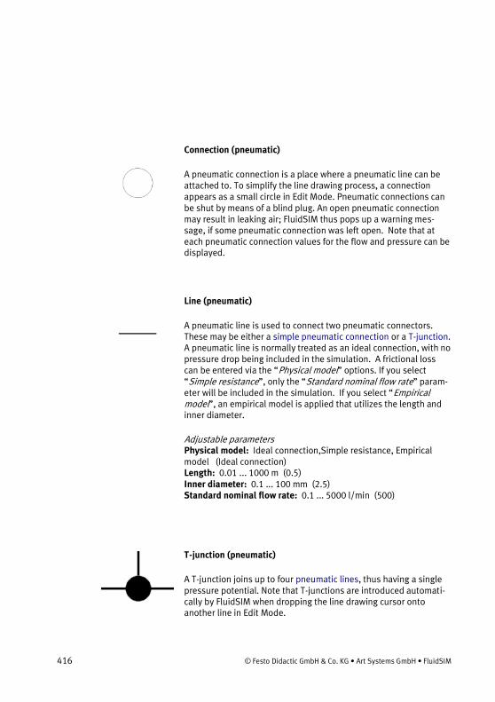
416 © Festo Didactic GmbH & Co. KG • Art Systems GmbH • FluidSIM
Connection (pneumatic)
A pneumatic connection is a place where a pneumatic line can be attached to. To simplify the line drawing process, a connection appears as a small circle in Edit Mode. Pneumatic connections can be shut by means of a blind plug. An open pneumatic connection may result in leaking air; FluidSIM thus pops up a warning mes-sage, if some pneumatic connection was left open. Note that at each pneumatic connection values for the flow and pressure can be displayed.
Line (pneumatic)
A pneumatic line is used to connect two pneumatic connectors. These may be either a simple pneumatic connection or a T-junction. A pneumatic line is normally treated as an ideal connection, with no pressure drop being included in the simulation. A frictional loss can be entered via the “Physical model” options. If you select “Simple resistance”, only the “Standard nominal flow rate” param-eter will be included in the simulation. If you select “Empirical model”, an empirical model is applied that utilizes the length and inner diameter.
Adjustable parameters Physical model: Ideal connection,Simple resistance, Empirical model (Ideal connection) Length: 0.01 ... 1000 m (0.5) Inner diameter: 0.1 ... 100 mm (2.5) Standard nominal flow rate: 0.1 ... 5000 l/min (500)
T-junction (pneumatic)
A T-junction joins up to four pneumatic lines, thus having a single pressure potential. Note that T-junctions are introduced automati-cally by FluidSIM when dropping the line drawing cursor onto another line in Edit Mode.

© Festo Didactic GmbH & Co. KG • Art Systems GmbH • FluidSIM 417
21.2.2 Configurable Way Valves
Configurable 2/n way valve
The configurable 2/n way valve is a way valve with two connec-tions, where both its body elements operation modes are user-definable.
Additionally, the pneumatic connections can be closed with either blind plugs or exhausts.
Adjustable parameters Desired position: 0 ... 4 (0) Standard nominal flow rate: 0.1 ... 5000 l/min (60) Positioning time: 1e-4 ... 10 s (0.02) Reset time: 1e-4 ... 10 s (0.03) Minimum voltage: 0.1 ... 300 V (20) Electrically left at U_min: 0.01 ... 100 N (70) Electrically right at U_min: 0.01 ... 100 N (70) Mechanically left: 0.01 ... 100 N (100) Mechanically right: 0.01 ... 100 N (100) Physical spring force: 0.01 ... 100 N (30) Minimum force: 0.01 ... 100 N (20) Min. pilot control force: 0.01 ... 100 N (15) Left: 0.01 ... 100 cm2 (1) Right: 0.01 ... 100 cm2 (1) Pilot control left: 0.01 ... 100 cm2 (1) Pilot control right: 0.01 ... 100 cm2 (1) air spring left: 0.01 ... 100 cm2 (0.5) air spring right: 0.01 ... 100 cm2 (0.5)
Configurable 3/n way valve
The configurable 3/n way valve is a way valve with two connec-tions, where both its body elements operation modes are user-definable.

418 © Festo Didactic GmbH & Co. KG • Art Systems GmbH • FluidSIM
Additionally, the pneumatic connections can be closed with either blind plugs or exhausts.
Adjustable parameters Desired position: 0 ... 4 (0) Standard nominal flow rate: 0.1 ... 5000 l/min (60) Positioning time: 1e-4 ... 10 s (0.02) Reset time: 1e-4 ... 10 s (0.03) Minimum voltage: 0.1 ... 300 V (20) Electrically left at U_min: 0.01 ... 100 N (70) Electrically right at U_min: 0.01 ... 100 N (70) Mechanically left: 0.01 ... 100 N (100) Mechanically right: 0.01 ... 100 N (100) Physical spring force: 0.01 ... 100 N (30) Minimum force: 0.01 ... 100 N (20) Min. pilot control force: 0.01 ... 100 N (15) Left: 0.01 ... 100 cm2 (1) Right: 0.01 ... 100 cm2 (1) Pilot control left: 0.01 ... 100 cm2 (1) Pilot control right: 0.01 ... 100 cm2 (1) air spring left: 0.01 ... 100 cm2 (0.5) air spring right: 0.01 ... 100 cm2 (0.5)
Configurable 4/n way valve
The configurable 4/n way valve is a way valve with two connec-tions, where both its body elements operation modes are user-definable.
Additionally, the pneumatic connections can be closed with either blind plugs or exhausts.
Adjustable parameters Desired position: 0 ... 4 (0) Standard nominal flow rate: 0.1 ... 5000 l/min (60) Positioning time: 1e-4 ... 10 s (0.02) Reset time: 1e-4 ... 10 s (0.03) Minimum voltage: 0.1 ... 300 V (20) Electrically left at U_min: 0.01 ... 100 N (70) Electrically right at U_min: 0.01 ... 100 N (70)

© Festo Didactic GmbH & Co. KG • Art Systems GmbH • FluidSIM 419
Mechanically left: 0.01 ... 100 N (100) Mechanically right: 0.01 ... 100 N (100) Physical spring force: 0.01 ... 100 N (30) Minimum force: 0.01 ... 100 N (20) Min. pilot control force: 0.01 ... 100 N (15) Left: 0.01 ... 100 cm2 (1) Right: 0.01 ... 100 cm2 (1) Pilot control left: 0.01 ... 100 cm2 (1) Pilot control right: 0.01 ... 100 cm2 (1) air spring left: 0.01 ... 100 cm2 (0.5) air spring right: 0.01 ... 100 cm2 (0.5)
Configurable 5/n way valve
The configurable 5/n way valve is a way valve with two connec-tions, where both its body elements operation modes are user-definable.
Additionally, the pneumatic connections can be closed with either blind plugs or exhausts.
Adjustable parameters Desired position: 0 ... 4 (0) Standard nominal flow rate: 0.1 ... 5000 l/min (60) Positioning time: 1e-4 ... 10 s (0.02) Reset time: 1e-4 ... 10 s (0.03) Minimum voltage: 0.1 ... 300 V (20) Electrically left at U_min: 0.01 ... 100 N (70) Electrically right at U_min: 0.01 ... 100 N (70) Mechanically left: 0.01 ... 100 N (100) Mechanically right: 0.01 ... 100 N (100) Physical spring force: 0.01 ... 100 N (30) Minimum force: 0.01 ... 100 N (20) Min. pilot control force: 0.01 ... 100 N (15) Left: 0.01 ... 100 cm2 (1) Right: 0.01 ... 100 cm2 (1) Pilot control left: 0.01 ... 100 cm2 (1) Pilot control right: 0.01 ... 100 cm2 (1) air spring left: 0.01 ... 100 cm2 (0.5)

420 © Festo Didactic GmbH & Co. KG • Art Systems GmbH • FluidSIM
air spring right: 0.01 ... 100 cm2 (0.5)
Configurable 6/n way valve
The configurable 6/n way valve is a way valve with two connec-tions, where both its body elements operation modes are user-definable.
Additionally, the pneumatic connections can be closed with either blind plugs or exhausts.
Adjustable parameters Desired position: 0 ... 4 (0) Standard nominal flow rate: 0.1 ... 5000 l/min (60) Positioning time: 1e-4 ... 10 s (0.02) Reset time: 1e-4 ... 10 s (0.03) Minimum voltage: 0.1 ... 300 V (20) Electrically left at U_min: 0.01 ... 100 N (70) Electrically right at U_min: 0.01 ... 100 N (70) Mechanically left: 0.01 ... 100 N (100) Mechanically right: 0.01 ... 100 N (100) Physical spring force: 0.01 ... 100 N (30) Minimum force: 0.01 ... 100 N (20) Min. pilot control force: 0.01 ... 100 N (15) Left: 0.01 ... 100 cm2 (1) Right: 0.01 ... 100 cm2 (1) Pilot control left: 0.01 ... 100 cm2 (1) Pilot control right: 0.01 ... 100 cm2 (1) air spring left: 0.01 ... 100 cm2 (0.5) air spring right: 0.01 ... 100 cm2 (0.5)
Configurable 8/n way valve
The configurable 8/n way valve is a way valve with two connec-tions, where both its body elements operation modes are user-definable.

© Festo Didactic GmbH & Co. KG • Art Systems GmbH • FluidSIM 421
Additionally, the pneumatic connections can be closed with either blind plugs or exhausts.
Adjustable parameters Desired position: 0 ... 4 (0) Standard nominal flow rate: 0.1 ... 5000 l/min (60) Positioning time: 1e-4 ... 10 s (0.02) Reset time: 1e-4 ... 10 s (0.03) Minimum voltage: 0.1 ... 300 V (20) Electrically left at U_min: 0.01 ... 100 N (70) Electrically right at U_min: 0.01 ... 100 N (70) Mechanically left: 0.01 ... 100 N (100) Mechanically right: 0.01 ... 100 N (100) Physical spring force: 0.01 ... 100 N (30) Minimum force: 0.01 ... 100 N (20) Min. pilot control force: 0.01 ... 100 N (15) Left: 0.01 ... 100 cm2 (1) Right: 0.01 ... 100 cm2 (1) Pilot control left: 0.01 ... 100 cm2 (1) Pilot control right: 0.01 ... 100 cm2 (1) air spring left: 0.01 ... 100 cm2 (0.5) air spring right: 0.01 ... 100 cm2 (0.5)
21.2.3 Mechanically Operated Directional Valves
3/2-way roller lever valve, normally closed
The roller lever valve is operated by pressing on the lever, for example through the use of a switching cam of a cylinder. The flow passes through from 1 to 2. After releasing the lever, the valve returns to its initial position through the use of a return spring. Connection 1 is shut. In the Simulation Mode, the valve can be switched manually by clicking on the component, thus not requiring a cylinder to operate the valve. This valve is derived from a config-

422 © Festo Didactic GmbH & Co. KG • Art Systems GmbH • FluidSIM
urable 3/n way valve. You find this valve in the component library
“Frequently used Way Valves”, under the Library menu.
Adjustable parameters Desired position: 0 ... 4 (0) Standard nominal flow rate: 0.1 ... 5000 l/min (60) Positioning time: 1e-4 ... 10 s (0.02) Reset time: 1e-4 ... 10 s (0.03) Minimum voltage: 0.1 ... 300 V (20) Electrically left at U_min: 0.01 ... 100 N (70) Electrically right at U_min: 0.01 ... 100 N (70) Mechanically left: 0.01 ... 100 N (100) Mechanically right: 0.01 ... 100 N (100) Physical spring force: 0.01 ... 100 N (30) Minimum force: 0.01 ... 100 N (20) Min. pilot control force: 0.01 ... 100 N (15) Left: 0.01 ... 100 cm2 (1) Right: 0.01 ... 100 cm2 (1) Pilot control left: 0.01 ... 100 cm2 (1) Pilot control right: 0.01 ... 100 cm2 (1) air spring left: 0.01 ... 100 cm2 (0.5) air spring right: 0.01 ... 100 cm2 (0.5)
3/2-way roller lever valve, normally open
The roller lever valve is operated by pressing on the lever, for example through the use of a switching cam of a cylinder. Connec-tion 1 is shut. After releasing the lever, the valve returns to its initial position through the use of a return spring. The flow may pass through freely from 1 to 2. In the Simulation Mode, the valve can be switched manually by clicking on the component, thus not requiring a cylinder to operate the valve. This valve is derived from a configurable 3/n way valve. You find this valve in the component
library “Frequently used Way Valves”, under the Library menu.
Adjustable parameters Desired position: 0 ... 4 (0) Standard nominal flow rate: 0.1 ... 5000 l/min (60) Positioning time: 1e-4 ... 10 s (0.02) Reset time: 1e-4 ... 10 s (0.03)

© Festo Didactic GmbH & Co. KG • Art Systems GmbH • FluidSIM 423
Minimum voltage: 0.1 ... 300 V (20) Electrically left at U_min: 0.01 ... 100 N (70) Electrically right at U_min: 0.01 ... 100 N (70) Mechanically left: 0.01 ... 100 N (100) Mechanically right: 0.01 ... 100 N (100) Physical spring force: 0.01 ... 100 N (30) Minimum force: 0.01 ... 100 N (20) Min. pilot control force: 0.01 ... 100 N (15) Left: 0.01 ... 100 cm2 (1) Right: 0.01 ... 100 cm2 (1) Pilot control left: 0.01 ... 100 cm2 (1) Pilot control right: 0.01 ... 100 cm2 (1) air spring left: 0.01 ... 100 cm2 (0.5) air spring right: 0.01 ... 100 cm2 (0.5)
3/2-way idle return roller valve, normally closed
The idle return roller valve is operated when the roller is driven in a specific direction by the switching cam of a cylinder. After releasing the roller, the valve returns to its initial position through the use of a return spring. Connection 1 is shut. When the roller is driven in the opposite direction, the valve is not operated. In the Simulation Mode, the valve can be switched manually by clicking on the com-ponent, thus not requiring a cylinder to operate the valve. This valve is derived from a configurable 3/n way valve. You find this valve in the component library “Frequently used Way Valves”,
under the Library menu.
Adjustable parameters Desired position: 0 ... 4 (0) Standard nominal flow rate: 0.1 ... 5000 l/min (60) Positioning time: 1e-4 ... 10 s (0.02) Reset time: 1e-4 ... 10 s (0.03) Minimum voltage: 0.1 ... 300 V (20) Electrically left at U_min: 0.01 ... 100 N (70) Electrically right at U_min: 0.01 ... 100 N (70) Mechanically left: 0.01 ... 100 N (100) Mechanically right: 0.01 ... 100 N (100) Physical spring force: 0.01 ... 100 N (30) Minimum force: 0.01 ... 100 N (20)

424 © Festo Didactic GmbH & Co. KG • Art Systems GmbH • FluidSIM
Min. pilot control force: 0.01 ... 100 N (15) Left: 0.01 ... 100 cm2 (1) Right: 0.01 ... 100 cm2 (1) Pilot control left: 0.01 ... 100 cm2 (1) Pilot control right: 0.01 ... 100 cm2 (1) air spring left: 0.01 ... 100 cm2 (0.5) air spring right: 0.01 ... 100 cm2 (0.5)
Pressurizing valve
The pressurizing valve with plunger control is operated by the surface of the cylinder cam. When the plunger is operated, com-pressed air flows freely until the nozzle is closed. A signal up to the level of the boost pressure is assembled at exit connection 2. In the Simulation Mode, the valve can be switched manually by click-ing on the component, thus not requiring a cylinder to operate the valve.
Adjustable parameters Desired position: 0 ... 4 (0) Standard nominal flow rate: 0.1 ... 5000 l/min (60) Positioning time: 1e-4 ... 10 s (0.02) Reset time: 1e-4 ... 10 s (0.03) Minimum voltage: 0.1 ... 300 V (20) Electrically left at U_min: 0.01 ... 100 N (70) Electrically right at U_min: 0.01 ... 100 N (70) Mechanically left: 0.01 ... 100 N (100) Mechanically right: 0.01 ... 100 N (100) Physical spring force: 0.01 ... 100 N (30) Minimum force: 0.01 ... 100 N (20) Min. pilot control force: 0.01 ... 100 N (15) Left: 0.01 ... 100 cm2 (1) Right: 0.01 ... 100 cm2 (1) Pilot control left: 0.01 ... 100 cm2 (1) Pilot control right: 0.01 ... 100 cm2 (1) air spring left: 0.01 ... 100 cm2 (0.5) air spring right: 0.01 ... 100 cm2 (0.5)

© Festo Didactic GmbH & Co. KG • Art Systems GmbH • FluidSIM 425
Pneumatic proximity switch, solenoid operated
A permanent solenoid found on the piston of a cylinder drives this 3/2 pneumatic directional valve and triggers the control signal. The flow passes freely from 1 to 2. In the Simulation Mode, the valve can be switched manually by clicking on the component, thus not requiring a cylinder to operate the valve. This valve is derived from a configurable 3/n way valve. You find this valve in the component
library “Frequently used Way Valves”, under the Library menu.
Adjustable parameters Desired position: 0 ... 4 (0) Standard nominal flow rate: 0.1 ... 5000 l/min (60) Positioning time: 1e-4 ... 10 s (0.02) Reset time: 1e-4 ... 10 s (0.03) Minimum voltage: 0.1 ... 300 V (20) Electrically left at U_min: 0.01 ... 100 N (70) Electrically right at U_min: 0.01 ... 100 N (70) Mechanically left: 0.01 ... 100 N (100) Mechanically right: 0.01 ... 100 N (100) Physical spring force: 0.01 ... 100 N (30) Minimum force: 0.01 ... 100 N (20) Min. pilot control force: 0.01 ... 100 N (15) Left: 0.01 ... 100 cm2 (1) Right: 0.01 ... 100 cm2 (1) Pilot control left: 0.01 ... 100 cm2 (1) Pilot control right: 0.01 ... 100 cm2 (1) air spring left: 0.01 ... 100 cm2 (0.5) air spring right: 0.01 ... 100 cm2 (0.5)
3/2-way valve with pushbutton, normally closed
Pressing the pushbutton operates the valve. The flow passes freely from 1 to 2. Releasing the pushbutton allows the valve to return to its starting position through the use of a return spring. Connection
1 is shut. By holding down the Shift key and simultaneously
clicking on the component with the mouse cursor, FluidSIM keeps the valve in permanent operating position. Simply clicking on the

426 © Festo Didactic GmbH & Co. KG • Art Systems GmbH • FluidSIM
component cancels the operated state and returns the valve to its starting position. This valve is derived from a configurable 3/n way valve. You find this valve in the component library “Frequently used
Way Valves”, under the Library menu.
Adjustable parameters Desired position: 0 ... 4 (0) Standard nominal flow rate: 0.1 ... 5000 l/min (60) Positioning time: 1e-4 ... 10 s (0.02) Reset time: 1e-4 ... 10 s (0.03) Minimum voltage: 0.1 ... 300 V (20) Electrically left at U_min: 0.01 ... 100 N (70) Electrically right at U_min: 0.01 ... 100 N (70) Mechanically left: 0.01 ... 100 N (100) Mechanically right: 0.01 ... 100 N (100) Physical spring force: 0.01 ... 100 N (30) Minimum force: 0.01 ... 100 N (20) Min. pilot control force: 0.01 ... 100 N (15) Left: 0.01 ... 100 cm2 (1) Right: 0.01 ... 100 cm2 (1) Pilot control left: 0.01 ... 100 cm2 (1) Pilot control right: 0.01 ... 100 cm2 (1) air spring left: 0.01 ... 100 cm2 (0.5) air spring right: 0.01 ... 100 cm2 (0.5)
3/2-way valve with pushbutton, normally open
Pressing the pushbutton operates the valve. Connection 1 is shut. Releasing the pushbutton allows the valve to returns to its starting position through the use of a return spring. The passes freely from
1 to 2. By holding down the Shift key and simultaneously click-
ing on the component with the mouse cursor, FluidSIM keeps the valve in permanent operating position. Simply clicking on the component cancels the operated state and returns the valve to its starting position. This valve is derived from a configurable 3/n way valve. You find this valve in the component library “Frequently used
Way Valves”, under the Library menu.
Adjustable parameters

© Festo Didactic GmbH & Co. KG • Art Systems GmbH • FluidSIM 427
Desired position: 0 ... 4 (0) Standard nominal flow rate: 0.1 ... 5000 l/min (60) Positioning time: 1e-4 ... 10 s (0.02) Reset time: 1e-4 ... 10 s (0.03) Minimum voltage: 0.1 ... 300 V (20) Electrically left at U_min: 0.01 ... 100 N (70) Electrically right at U_min: 0.01 ... 100 N (70) Mechanically left: 0.01 ... 100 N (100) Mechanically right: 0.01 ... 100 N (100) Physical spring force: 0.01 ... 100 N (30) Minimum force: 0.01 ... 100 N (20) Min. pilot control force: 0.01 ... 100 N (15) Left: 0.01 ... 100 cm2 (1) Right: 0.01 ... 100 cm2 (1) Pilot control left: 0.01 ... 100 cm2 (1) Pilot control right: 0.01 ... 100 cm2 (1) air spring left: 0.01 ... 100 cm2 (0.5) air spring right: 0.01 ... 100 cm2 (0.5)
3/2-way valve with selection switch or striking button
Pressing the red striking button operates the valve. The flow passes freely from 1 to 2. Releasing the button has no effect; the valve remains in its operating position. Turning the button to the right sets the striking button back to its original position and the valve returns to its starting position through the use of a return spring. Connection 1 is shut. This valve is derived from a configurable 3/n way valve. You find this valve in the component library “Frequently
used Way Valves”, under the Library menu.
Adjustable parameters Desired position: 0 ... 4 (0) Standard nominal flow rate: 0.1 ... 5000 l/min (60) Positioning time: 1e-4 ... 10 s (0.02) Reset time: 1e-4 ... 10 s (0.03) Minimum voltage: 0.1 ... 300 V (20) Electrically left at U_min: 0.01 ... 100 N (70) Electrically right at U_min: 0.01 ... 100 N (70) Mechanically left: 0.01 ... 100 N (100) Mechanically right: 0.01 ... 100 N (100)

428 © Festo Didactic GmbH & Co. KG • Art Systems GmbH • FluidSIM
Physical spring force: 0.01 ... 100 N (30) Minimum force: 0.01 ... 100 N (20) Min. pilot control force: 0.01 ... 100 N (15) Left: 0.01 ... 100 cm2 (1) Right: 0.01 ... 100 cm2 (1) Pilot control left: 0.01 ... 100 cm2 (1) Pilot control right: 0.01 ... 100 cm2 (1) air spring left: 0.01 ... 100 cm2 (0.5) air spring right: 0.01 ... 100 cm2 (0.5)
5/2-way valve, with selection switch
Turning the selection switch operates the valve. The flow passes freely from 1 to 4. Releasing the switch has no effect; the valve remains in its operating position. Turning the switch back to its original position allows the flow to pass freely from 1 to 2. This valve is derived from a configurable 5/n way valve. You find this valve in the component library “Frequently used Way Valves”,
under the Library menu.
Adjustable parameters Desired position: 0 ... 4 (0) Standard nominal flow rate: 0.1 ... 5000 l/min (60) Positioning time: 1e-4 ... 10 s (0.02) Reset time: 1e-4 ... 10 s (0.03) Minimum voltage: 0.1 ... 300 V (20) Electrically left at U_min: 0.01 ... 100 N (70) Electrically right at U_min: 0.01 ... 100 N (70) Mechanically left: 0.01 ... 100 N (100) Mechanically right: 0.01 ... 100 N (100) Physical spring force: 0.01 ... 100 N (30) Minimum force: 0.01 ... 100 N (20) Min. pilot control force: 0.01 ... 100 N (15) Left: 0.01 ... 100 cm2 (1) Right: 0.01 ... 100 cm2 (1) Pilot control left: 0.01 ... 100 cm2 (1) Pilot control right: 0.01 ... 100 cm2 (1) air spring left: 0.01 ... 100 cm2 (0.5) air spring right: 0.01 ... 100 cm2 (0.5)

© Festo Didactic GmbH & Co. KG • Art Systems GmbH • FluidSIM 429
21.2.4 Solenoid Operated Directional Valves
3/2-way solenoid valve, normally closed
The solenoid valve is controlled by applying a voltage signal at the solenoid coil. The flow passes freely from 1 to 2. By stopping the signal the valve is set back to its starting position through the use of a return spring. Connection 1 is shut. If no signal is applied to the valve, it can be manually operated. This valve is derived from a configurable 3/n way valve. You find this valve in the component
library “Frequently used Way Valves”, under the Library menu.
Adjustable parameters Desired position: 0 ... 4 (0) Standard nominal flow rate: 0.1 ... 5000 l/min (60) Positioning time: 1e-4 ... 10 s (0.02) Reset time: 1e-4 ... 10 s (0.03) Minimum voltage: 0.1 ... 300 V (20) Electrically left at U_min: 0.01 ... 100 N (70) Electrically right at U_min: 0.01 ... 100 N (70) Mechanically left: 0.01 ... 100 N (100) Mechanically right: 0.01 ... 100 N (100) Physical spring force: 0.01 ... 100 N (30) Minimum force: 0.01 ... 100 N (20) Min. pilot control force: 0.01 ... 100 N (15) Left: 0.01 ... 100 cm2 (1) Right: 0.01 ... 100 cm2 (1) Pilot control left: 0.01 ... 100 cm2 (1) Pilot control right: 0.01 ... 100 cm2 (1) air spring left: 0.01 ... 100 cm2 (0.5) air spring right: 0.01 ... 100 cm2 (0.5)

430 © Festo Didactic GmbH & Co. KG • Art Systems GmbH • FluidSIM
3/2-way solenoid valve, normally open
The solenoid valve is controlled by applying a voltage signal at the solenoid coil. Connection 1 is shut. By stopping the signal the valve is set back to its starting position through the use of a return spring. The flow passes freely from 1 to 2. If no signal is applied to the valve, it can be manually operated. This valve is derived from a configurable 3/n way valve. You find this valve in the component
library “Frequently used Way Valves”, under the Library menu.
Adjustable parameters Desired position: 0 ... 4 (0) Standard nominal flow rate: 0.1 ... 5000 l/min (60) Positioning time: 1e-4 ... 10 s (0.02) Reset time: 1e-4 ... 10 s (0.03) Minimum voltage: 0.1 ... 300 V (20) Electrically left at U_min: 0.01 ... 100 N (70) Electrically right at U_min: 0.01 ... 100 N (70) Mechanically left: 0.01 ... 100 N (100) Mechanically right: 0.01 ... 100 N (100) Physical spring force: 0.01 ... 100 N (30) Minimum force: 0.01 ... 100 N (20) Min. pilot control force: 0.01 ... 100 N (15) Left: 0.01 ... 100 cm2 (1) Right: 0.01 ... 100 cm2 (1) Pilot control left: 0.01 ... 100 cm2 (1) Pilot control right: 0.01 ... 100 cm2 (1) air spring left: 0.01 ... 100 cm2 (0.5) air spring right: 0.01 ... 100 cm2 (0.5)
5/2-way solenoid valve
The solenoid valve is controlled by applying a voltage signal at the solenoid coil. The flow passes freely from 1 to 4. By stopping the signal the valve is set back to its starting position through the use of a return spring. The flow passes freely from 1 to 2. If no signal is applied to the valve, it can be manually operated. This valve is derived from a configurable 5/n way valve. You find this valve in

© Festo Didactic GmbH & Co. KG • Art Systems GmbH • FluidSIM 431
the component library “Frequently used Way Valves”, under the
Library menu.
Adjustable parameters Desired position: 0 ... 4 (0) Standard nominal flow rate: 0.1 ... 5000 l/min (60) Positioning time: 1e-4 ... 10 s (0.02) Reset time: 1e-4 ... 10 s (0.03) Minimum voltage: 0.1 ... 300 V (20) Electrically left at U_min: 0.01 ... 100 N (70) Electrically right at U_min: 0.01 ... 100 N (70) Mechanically left: 0.01 ... 100 N (100) Mechanically right: 0.01 ... 100 N (100) Physical spring force: 0.01 ... 100 N (30) Minimum force: 0.01 ... 100 N (20) Min. pilot control force: 0.01 ... 100 N (15) Left: 0.01 ... 100 cm2 (1) Right: 0.01 ... 100 cm2 (1) Pilot control left: 0.01 ... 100 cm2 (1) Pilot control right: 0.01 ... 100 cm2 (1) air spring left: 0.01 ... 100 cm2 (0.5) air spring right: 0.01 ... 100 cm2 (0.5)
5/2-way solenoid impulse valve
The solenoid valve is controlled by applying a voltage signal at the solenoid coil (flow passes from 1 to 4) and remains in this operat-ing position even when the signal is cut off. Only by applying an opposite signal will the valve return to its starting position (flow passes freely from 1 to 2). If no signal is applied to the valve, it can be manually operated. This valve is derived from a configurable 5/n way valve. You find this valve in the component library “Fre-
quently used Way Valves”, under the Library menu.
Adjustable parameters Desired position: 0 ... 4 (0) Standard nominal flow rate: 0.1 ... 5000 l/min (60) Positioning time: 1e-4 ... 10 s (0.02) Reset time: 1e-4 ... 10 s (0.03) Minimum voltage: 0.1 ... 300 V (20)

432 © Festo Didactic GmbH & Co. KG • Art Systems GmbH • FluidSIM
Electrically left at U_min: 0.01 ... 100 N (70) Electrically right at U_min: 0.01 ... 100 N (70) Mechanically left: 0.01 ... 100 N (100) Mechanically right: 0.01 ... 100 N (100) Physical spring force: 0.01 ... 100 N (30) Minimum force: 0.01 ... 100 N (20) Min. pilot control force: 0.01 ... 100 N (15) Left: 0.01 ... 100 cm2 (1) Right: 0.01 ... 100 cm2 (1) Pilot control left: 0.01 ... 100 cm2 (1) Pilot control right: 0.01 ... 100 cm2 (1) air spring left: 0.01 ... 100 cm2 (0.5) air spring right: 0.01 ... 100 cm2 (0.5)
5/3-way solenoid valve, mid-Position closed
The solenoid valve is controlled by applying a voltage signal at the solenoid coil (flow passes from 1 to 4 or from 1 to 2). By stopping the signal the valve is set back to its starting position through the use of a return spring. Connections 1, 2, and 4 are shut. If no signal is applied to the valve, it can be manually operated. This valve is derived from a configurable 5/n way valve. You find this valve in the component library “Frequently used Way Valves”, under the
Library menu.
Adjustable parameters Desired position: 0 ... 4 (0) Standard nominal flow rate: 0.1 ... 5000 l/min (60) Positioning time: 1e-4 ... 10 s (0.02) Reset time: 1e-4 ... 10 s (0.03) Minimum voltage: 0.1 ... 300 V (20) Electrically left at U_min: 0.01 ... 100 N (70) Electrically right at U_min: 0.01 ... 100 N (70) Mechanically left: 0.01 ... 100 N (100) Mechanically right: 0.01 ... 100 N (100) Physical spring force: 0.01 ... 100 N (30) Minimum force: 0.01 ... 100 N (20) Min. pilot control force: 0.01 ... 100 N (15) Left: 0.01 ... 100 cm2 (1) Right: 0.01 ... 100 cm2 (1)

© Festo Didactic GmbH & Co. KG • Art Systems GmbH • FluidSIM 433
Pilot control left: 0.01 ... 100 cm2 (1) Pilot control right: 0.01 ... 100 cm2 (1) air spring left: 0.01 ... 100 cm2 (0.5) air spring right: 0.01 ... 100 cm2 (0.5)
21.2.5 Pneumatically Operated Directional Valves
3/2-way valve, pneumatically operated, normally closed
The pneumatic valve is controlled by applying a pilot pressure at connection 12. The flow passes freely from 1 to 2. By stopping the signal the valve is set back to its starting position through the use of a return spring. Connection 1 is shut. This valve is derived from a configurable 3/n way valve. You find this valve in the component
library “Frequently used Way Valves”, under the Library menu.
Adjustable parameters Desired position: 0 ... 4 (0) Standard nominal flow rate: 0.1 ... 5000 l/min (60) Positioning time: 1e-4 ... 10 s (0.02) Reset time: 1e-4 ... 10 s (0.03) Minimum voltage: 0.1 ... 300 V (20) Electrically left at U_min: 0.01 ... 100 N (70) Electrically right at U_min: 0.01 ... 100 N (70) Mechanically left: 0.01 ... 100 N (100) Mechanically right: 0.01 ... 100 N (100) Physical spring force: 0.01 ... 100 N (30) Minimum force: 0.01 ... 100 N (20) Min. pilot control force: 0.01 ... 100 N (15) Left: 0.01 ... 100 cm2 (1) Right: 0.01 ... 100 cm2 (1) Pilot control left: 0.01 ... 100 cm2 (1) Pilot control right: 0.01 ... 100 cm2 (1) air spring left: 0.01 ... 100 cm2 (0.5)

434 © Festo Didactic GmbH & Co. KG • Art Systems GmbH • FluidSIM
air spring right: 0.01 ... 100 cm2 (0.5)
3/2-way valve, pneumatically operated, normally open
The pneumatic valve is controlled by applying a pilot pressure at connection 10. Connection 1 is shut. By stopping the signal the valve is set back to its starting position through the use of a return spring. The flow passes freely from 1 to 2. This valve is derived from a configurable 3/n way valve. You find this valve in the component
library “Frequently used Way Valves”, under the Library menu.
Adjustable parameters Desired position: 0 ... 4 (0) Standard nominal flow rate: 0.1 ... 5000 l/min (60) Positioning time: 1e-4 ... 10 s (0.02) Reset time: 1e-4 ... 10 s (0.03) Minimum voltage: 0.1 ... 300 V (20) Electrically left at U_min: 0.01 ... 100 N (70) Electrically right at U_min: 0.01 ... 100 N (70) Mechanically left: 0.01 ... 100 N (100) Mechanically right: 0.01 ... 100 N (100) Physical spring force: 0.01 ... 100 N (30) Minimum force: 0.01 ... 100 N (20) Min. pilot control force: 0.01 ... 100 N (15) Left: 0.01 ... 100 cm2 (1) Right: 0.01 ... 100 cm2 (1) Pilot control left: 0.01 ... 100 cm2 (1) Pilot control right: 0.01 ... 100 cm2 (1) air spring left: 0.01 ... 100 cm2 (0.5) air spring right: 0.01 ... 100 cm2 (0.5)
5/2-way valve, pneumatically operated
The pneumatic valve is controlled by applying a pilot pressure at connection 14. The flow passes freely from 1 to 4. By stopping the signal the valve is set back to its starting position through the use of a return spring. The flow passes freely from 1 to 2. This valve is

© Festo Didactic GmbH & Co. KG • Art Systems GmbH • FluidSIM 435
derived from a configurable 5/n way valve. You find this valve in the component library “Frequently used Way Valves”, under the
Library menu.
Adjustable parameters Desired position: 0 ... 4 (0) Standard nominal flow rate: 0.1 ... 5000 l/min (60) Positioning time: 1e-4 ... 10 s (0.02) Reset time: 1e-4 ... 10 s (0.03) Minimum voltage: 0.1 ... 300 V (20) Electrically left at U_min: 0.01 ... 100 N (70) Electrically right at U_min: 0.01 ... 100 N (70) Mechanically left: 0.01 ... 100 N (100) Mechanically right: 0.01 ... 100 N (100) Physical spring force: 0.01 ... 100 N (30) Minimum force: 0.01 ... 100 N (20) Min. pilot control force: 0.01 ... 100 N (15) Left: 0.01 ... 100 cm2 (1) Right: 0.01 ... 100 cm2 (1) Pilot control left: 0.01 ... 100 cm2 (1) Pilot control right: 0.01 ... 100 cm2 (1) air spring left: 0.01 ... 100 cm2 (0.5) air spring right: 0.01 ... 100 cm2 (0.5)
5/2-way impulse valve, pneumatically operated
The pneumatic valve is controlled by applying reciprocal pilot pressures at connection 14 (flow passes from 1 to 4) and connec-tion 12 (flow passes from 1 to 2). The valve’s operating position remains until an opposite signal is received by the valve. This valve is derived from a configurable 5/n way valve. You find this valve in the component library “Frequently used Way Valves”, under the
Library menu.
Adjustable parameters Desired position: 0 ... 4 (0) Standard nominal flow rate: 0.1 ... 5000 l/min (60) Positioning time: 1e-4 ... 10 s (0.02) Reset time: 1e-4 ... 10 s (0.03) Minimum voltage: 0.1 ... 300 V (20)

436 © Festo Didactic GmbH & Co. KG • Art Systems GmbH • FluidSIM
Electrically left at U_min: 0.01 ... 100 N (70) Electrically right at U_min: 0.01 ... 100 N (70) Mechanically left: 0.01 ... 100 N (100) Mechanically right: 0.01 ... 100 N (100) Physical spring force: 0.01 ... 100 N (30) Minimum force: 0.01 ... 100 N (20) Min. pilot control force: 0.01 ... 100 N (15) Left: 0.01 ... 100 cm2 (1) Right: 0.01 ... 100 cm2 (1) Pilot control left: 0.01 ... 100 cm2 (1) Pilot control right: 0.01 ... 100 cm2 (1) air spring left: 0.01 ... 100 cm2 (0.5) air spring right: 0.01 ... 100 cm2 (0.5)
5/3-way pneumatic valve, mid-Position closed
The pneumatic valve is controlled by applying reciprocal pilot pressures at connection 14 (flow passes from 1 to 4) and connec-tion 12 (flow passes from 1 to 2). By stopping the signals the valve is set back to its starting position through the use of a return spring. Connections 1, 2, and 4 are shut. This valve is derived from a configurable 5/n way valve. You find this valve in the component
library “Frequently used Way Valves”, under the Library menu.
Adjustable parameters Desired position: 0 ... 4 (0) Standard nominal flow rate: 0.1 ... 5000 l/min (60) Positioning time: 1e-4 ... 10 s (0.02) Reset time: 1e-4 ... 10 s (0.03) Minimum voltage: 0.1 ... 300 V (20) Electrically left at U_min: 0.01 ... 100 N (70) Electrically right at U_min: 0.01 ... 100 N (70) Mechanically left: 0.01 ... 100 N (100) Mechanically right: 0.01 ... 100 N (100) Physical spring force: 0.01 ... 100 N (30) Minimum force: 0.01 ... 100 N (20) Min. pilot control force: 0.01 ... 100 N (15) Left: 0.01 ... 100 cm2 (1) Right: 0.01 ... 100 cm2 (1) Pilot control left: 0.01 ... 100 cm2 (1)

© Festo Didactic GmbH & Co. KG • Art Systems GmbH • FluidSIM 437
Pilot control right: 0.01 ... 100 cm2 (1) air spring left: 0.01 ... 100 cm2 (0.5) air spring right: 0.01 ... 100 cm2 (0.5)
Low pressure amplifier unit, 2 compartments
Each of the two double-level low pressure amplifier units has the function of a 3/2 directional valve that is normally closed. The signal at connection 12 is raised to a higher boost pressure level through the use of a double-level amplifier and is put out by con-nection 2.
Adjustable parameters Standard nominal flow rate: 0.1 ... 5000 l/min (60)
21.2.6 Shutoff Valves and Flow Control Valves
Shuttle valve
The shuttle valve is switched based on the compressed air entering into either input connection 1 and leaving via an output connection 2. Should both input connections begin receiving compressed air, the connection with the higher pressure takes precedence and is put out (OR function).
Adjustable parameters Standard nominal flow rate: 0.1 ... 5000 l/min (108)

438 © Festo Didactic GmbH & Co. KG • Art Systems GmbH • FluidSIM
Quick exhaust valve
The compressed air passes from connection 1 to connection 2. If the pressure should decrease at connection 1, then the com-pressed air from connection 2 will escape to the outside via the installed silencer.
Adjustable parameters Standard nominal flow rate 1...2: 0.1 ... 5000 l/min (300) Standard nominal flow rate 2...3: 0.1 ... 5000 l/min (550)
Two pressure valve
The two pressure valve is switched based on the compressed air entering into both input connections 1 and leaving via an output connection 2. Should both input connections begin receiving com-pressed air, the connection with the lower pressure takes prece-dence and is put out (AND function).
Adjustable parameters Standard nominal flow rate: 0.1 ... 5000 l/min (550)
Check valve
If the inlet pressure at 1 is higher than the outlet pressure at 2, then the check valve allows the flow to pass, otherwise it blocks the flow.
Adjustable parameters Standard nominal flow rate: 0.1 ... 5000 l/min (108)

© Festo Didactic GmbH & Co. KG • Art Systems GmbH • FluidSIM 439
Check valve, spring loaded
If the inlet pressure at 1 is higher than the outlet pressure at 2 and the nominal pressure, then the check valve allows the flow to pass, otherwise it blocks the flow.
Adjustable parameters Opening pressure: 0 ... 2 MPa (0.1) Pressure regulation range: 0.01 ... 1 MPa (0.05) Standard nominal flow rate: 0.1 ... 5000 l/min (108)
Check valve with pilot control
If the entering pressure at connection 1 is higher that the outgoing pressure at 2, the check valve allows the flow to pass freely. Other-wise, the valve stops the flow. Additionally, the check valve can be opened via the control line 12. This action allows the flow to pass freely in both directions.
Adjustable parameters Area ratio: 0.1 ... 10 (3.3) Standard nominal flow rate: 0.1 ... 5000 l/min (108)
Check valve with pilot control, spring loaded
If the inlet pressure at 1 is higher than the outlet pressure at 2 and the nominal pressure, then the check valve allows the flow to pass, otherwise it blocks the flow. Additionally, the check valve can be released using the pilot line 12, thus enabling the flow in both directions.
Adjustable parameters Opening pressure: 0 ... 2 MPa (0.1) Pressure regulation range: 0.01 ... 1 MPa (0.05) Area ratio: 0.1 ... 10 (3.3)

440 © Festo Didactic GmbH & Co. KG • Art Systems GmbH • FluidSIM
Standard nominal flow rate: 0.1 ... 5000 l/min (108)
Pilot to close check valve
If the inlet pressure at 1 is higher than the outlet pressure at 2, then the non-return valve allows the flow to pass, otherwise it blocks the flow. Additionally, the non-return valve can be closed using the pilot line 10.
Adjustable parameters Area ratio: 0.1 ... 10 (3.3) Standard nominal flow rate: 0.1 ... 5000 l/min (108)
Pilot to close check valve, spring loaded
If the inlet pressure at 1 is higher than the outlet pressure at 2 and the nominal pressure, then the non-return valve allows the flow to pass, otherwise it blocks the flow. Additionally, the non-return valve can be closed using the pilot line 10.
Adjustable parameters Opening pressure: 0 ... 2 MPa (0.1) Pressure regulation range: 0.01 ... 1 MPa (0.05) Area ratio: 0.1 ... 10 (3.3) Standard nominal flow rate: 0.1 ... 5000 l/min (108)
Nozzle
The nozzle represents a pneumatic resistance.
Adjustable parameters Standard nominal flow rate: 0.1 ... 5000 l/min (100)

© Festo Didactic GmbH & Co. KG • Art Systems GmbH • FluidSIM 441
Throttle valve
The setting of the throttle valve is set by means of a rotary knob. Please note that by the rotary knob no absolute resistance value can be set. This means that, in reality, different throttle valves can generate different resistance values despite identical settings.
Adjustable parameters Opening level: 0 ... 100 % (100) Standard nominal flow rate: 0.1 ... 5000 l/min (100)
Orifice
The orifice represents a pneumatic resistance.
Adjustable parameters Standard nominal flow rate: 0.1 ... 5000 l/min (100)
Orifice, adjustable
The orifice represents a variable pneumatic resistance.
Adjustable parameters Opening level: 0 ... 100 % (100) Standard nominal flow rate: 0.1 ... 5000 l/min (100)
One-way flow control valve
The one-way flow control valve is made up of a throttle valve and a check valve. The check valve stops the flow from passing in a cer-tain direction. The flow then passes though the throttle valve. The

442 © Festo Didactic GmbH & Co. KG • Art Systems GmbH • FluidSIM
cross-section of the throttle is adjustable via a regular screw. In the opposite direction the flow can pass through the check valve.
Adjustable parameters Opening level: 0 ... 100 % (100) Standard nominal flow rate (Flow control valve): 0.1 ... 5000 l/min (45) Standard nominal flow rate (Non-return valve): 0.1 ... 5000 l/min (65)
Pneumatic counter
The counter registers pneumatic signals starting at a predeter-mined number and counting backwards. If zero is reached, then the counter releases an output signal. This output signal continues until the counter is reset either by hand or from at signal at connec-tion 10.
Adjustable parameters Counter: 0 ... 9999 (3) Standard nominal flow rate: 0.1 ... 5000 l/min (60)
Time delay valve, normally closed
The time delay valve is actuated by a pneumatic signal at port 1 after a preset time delay has elapsed. It is returned to the normal position via return spring when the signal is removed. The time delay is infinitely adjustable by means of a regulating screw. The time delay is reset automatically within 200 ms.
Adjustable parameters Delay time: 0.1 ... 100 s (3) Standard nominal flow rate: 0.1 ... 5000 l/min (50)

© Festo Didactic GmbH & Co. KG • Art Systems GmbH • FluidSIM 443
Time delay valve, normally open
After the pilot signal is applied at port 10, a preset time elapses before the pneumatic timer is actuated. It returns to its initial position via a return spring once the signal is removed. The time delay is infinitely adjustable by means of a regulating screw. The time delay is reset automatically within 200 ms.
Adjustable parameters Delay time: 0.1 ... 100 s (3) Standard nominal flow rate: 0.1 ... 5000 l/min (50)
Ring sensor
The ring sensor is a non-contact pneumatic signal output module. It is supplied with low pressure at connection 1. If, due to an object, the entering air flow is disturbed, a low pressure signal will be put out by connection 2. To simulate an object in the air flow, as pre-sented above, simply click on the component during FluidSIM Simulation Mode.
21.2.7 Pressure Operated Switches
2-way pressure regulator valve
The pressure regulator valve regulates the compressed air supply to the preset nominal pressure and equalizes pressure fluctuations. The valve closes when the pressure at connection 2 exceeds the nominal pressure. The setting for the real components is compo-nent dependent and cannot be changed.
Adjustable parameters

444 © Festo Didactic GmbH & Co. KG • Art Systems GmbH • FluidSIM
Nominal pressure: 0 ... 2 MPa (0.4) Pressure regulation range: 0.01 ... 1 MPa (0.05) Standard nominal flow rate: 0.1 ... 5000 l/min (300)
2-way pressure regulator valve, adjustable
The pressure regulator valve regulates the compressed air supply to the preset nominal pressure and equalizes pressure fluctuations. The valve closes when the pressure at connection 2 exceeds the nominal pressure.
Adjustable parameters Nominal pressure: 0 ... 2 MPa (0.4) Pressure regulation range: 0.01 ... 1 MPa (0.05) Standard nominal flow rate: 0.1 ... 5000 l/min (300)
Pressure regulator valve with manometer
The pressure control valve regulates the supplied pressure based on the adjustable operating pressure and the variations in the pressure. The manometer displays the pressure at connection 2.
Adjustable parameters Nominal pressure: 0 ... 2 MPa (0.4) Pressure regulation range: 0.01 ... 1 MPa (0.05) Standard nominal flow rate: 0.1 ... 5000 l/min (300)
3-way pressure regulator valve
The pressure regulator valve regulates the compressed air supply to the preset nominal pressure and equalizes pressure fluctuations. The compressed air is discharged via connection 3 when the pres-sure at connection 2 exceeds the nominal pressure. The setting for

© Festo Didactic GmbH & Co. KG • Art Systems GmbH • FluidSIM 445
the real components is component dependent and cannot be changed.
Adjustable parameters Nominal pressure: 0 ... 2 MPa (0.4) Pressure regulation range: 0.01 ... 1 MPa (0.05) Standard nominal flow rate: 0.1 ... 5000 l/min (300)
3-way pressure regulator valve, adjustable
The pressure regulator valve regulates the compressed air supply to the preset nominal pressure and equalizes pressure fluctuations. The compressed air is discharged via connection 3 when the pres-sure at connection 2 exceeds the nominal pressure.
Adjustable parameters Nominal pressure: 0 ... 2 MPa (0.4) Pressure regulation range: 0.01 ... 1 MPa (0.05) Standard nominal flow rate: 0.1 ... 5000 l/min (300)
Closing pressure compensator
The pressure compensator represents a pressure dependent pneumatic resistance. The pressure compensator closes when the pressure difference p3-p4 exceeds the nominal pressure. A pres-sure regulating valve is implemented by the combination of connec-tions 2 and 3. The nominal pressure setting of the real components is component dependent and cannot be changed.
Adjustable parameters Nominal pressure: 0 ... 2 MPa (0.4) Pressure regulation range: 0.01 ... 1 MPa (0.05) Standard nominal flow rate: 0.1 ... 5000 l/min (300)

446 © Festo Didactic GmbH & Co. KG • Art Systems GmbH • FluidSIM
Closing pressure compensator, adjustable
The pressure compensator represents a pressure dependent pneumatic resistance. The pressure compensator closes when the pressure difference p3-p4 exceeds the nominal pressure. A pres-sure regulating valve is implemented by the combination of connec-tions 2 and 3.
Adjustable parameters Nominal pressure: 0 ... 2 MPa (0.4) Pressure regulation range: 0.01 ... 1 MPa (0.05) Standard nominal flow rate: 0.1 ... 5000 l/min (300)
Opening pressure compensator
The pressure compensator represents a pressure dependent pneumatic resistance. The pressure compensator opens when the pressure difference p3-p4 exceeds the nominal pressure. A se-quence valve is implemented by the combination of connections 1 and 3. The nominal pressure setting of the real components is component dependent and cannot be changed.
Adjustable parameters Nominal pressure: 0 ... 2 MPa (0.4) Pressure regulation range: 0.01 ... 1 MPa (0.05) Standard nominal flow rate: 0.1 ... 5000 l/min (300)
Opening pressure compensator, adjustable
The pressure compensator represents a pressure dependent pneumatic resistance. The pressure compensator opens when the pressure difference p3-p4 exceeds the nominal pressure. A se-quence valve is implemented by the combination of connections 1 and 3.

© Festo Didactic GmbH & Co. KG • Art Systems GmbH • FluidSIM 447
Adjustable parameters Nominal pressure: 0 ... 2 MPa (0.4) Pressure regulation range: 0.01 ... 1 MPa (0.05) Standard nominal flow rate: 0.1 ... 5000 l/min (300)
21.2.8 Pressure Operated Switches
Analog pressure sensor
The pressure sensor measures the pressure and operates the pressure switch when the adjustable switching pressure has been exceeded.
Adjustable parameters Switching pressure: -0.1 ... 2 MPa (0.3) Hysteresis: 0 ... 1 MPa (0)
Vacuum switch
The vacuum switch operates the linked pressure switch, when the pressure falls below the adjustable switching pressure. If the sym-bol is used as a pressure switch the respective switch is operated when the pressure exceeds the switching pressure.
Adjustable parameters Switching pressure: -0.1 ... 2 MPa (0.3) Hysteresis: 0 ... 1 MPa (0)

448 © Festo Didactic GmbH & Co. KG • Art Systems GmbH • FluidSIM
Differential pressure switch
The differential pressure switch can be employed as a pressure switch (connection P1), a vacuum switch (connection P2) or as a differential pressure switch (P1-P2). The respective pneumatic to electric converter is operated when the difference in pressure between P1-P2 exceeds the adjustable switching pressure.
Adjustable parameters Switching pressure: -2 ... 2 MPa (0.3) Hysteresis: 0 ... 1 MPa (0)
21.2.9 Vacuum Technique
Vacuum suction nozzle
The vacuum suction nozzle creates its vacuum based on the ejector principle. In this case, compressed air flows from connection 1 to 3, creating a vacuum at connection 1v. A sucker can be connected to the vacuum connection 1v. Stopping the input of compressed air at connection 1 stops any suction also.
Adjustable parameters Maximum vacuum: -0.999 ... 0 bar (-0.85) Operating pressure for max. vacuum: 0.1 ... 20 bar (4.25) Air consumption at 600 kPa: 1 ... 1000 l/min (11.6) Max. suction rate: 0.1 ... 1000 l/min (6)

© Festo Didactic GmbH & Co. KG • Art Systems GmbH • FluidSIM 449
Vacuum suction nozzle
The vacuum suction nozzle creates its vacuum based on the ejector principle. In this case, compressed air flows from connection 1 to 3, creating a vacuum at connection 1v. A sucker can be connected to the vacuum connection 1v. Stopping the input of compressed air at connection 1 stops any suction also.
Adjustable parameters Maximum vacuum: -0.999 ... 0 bar (-0.85) Operating pressure for max. vacuum: 0.1 ... 20 bar (4.25) Air consumption at 600 kPa: 1 ... 1000 l/min (11.6) Max. suction rate: 0.1 ... 1000 l/min (6)
Single-stage ejector with repulsion mechanism (vacuum genera-tor)
The vacuum generator functions like the vacuum suction nozzle, except that an integrated reservoir is filled with air during the suction process. When the input line is switched off, the com-pressed air stored in the reservoir discharges in a pulse via the port (quick exhaust), securely repelling the suctioned workpiece from the vacuum cup. The volume can be enlarged by means of an additional port. This additional volume allows the energy of the vent pulse to be varied as required.
Adjustable parameters Maximum vacuum: -0.999 ... 0 bar (-0.85) Operating pressure for max. vacuum: 0.1 ... 20 bar (4.25) Air consumption at 600 kPa: 1 ... 1000 l/min (11.6) Max. suction rate: 0.1 ... 1000 l/min (6) Volume: 0.001 ... 10 l (0.05)

450 © Festo Didactic GmbH & Co. KG • Art Systems GmbH • FluidSIM
Suction cup
The suction cup can be used together with the vacuum suction nozzle to grip objects by suction. Lowering the cup onto an object is simulated in FluidSIM in Simulation Mode by clicking on the component. An additional click lifts the suction cup.
Adjustable parameters Diameter: 1 ... 1000 mm (20) Load to be lifted: 0.001 ... 1000 kg (0.1) Safety factor: 0.1 ... 100 (1)
Vacuum security valve
If multiple suction cups are supplied with vacuum by one vacuum suction nozzle, the vacuum will collapse if one or more cups do not form a suction grip on the workpiece or workpieces. To prevent this, so-called vacuum security valves are used. Vacuum security valves are installed between the vacuum suction nozzle and the suction cup. If, during vacuum generation, a suction cup is uncov-ered, or only partly covered, the vacuum security valve automatical-ly stops the influx of air. If the suction cup is open to the environ-ment, the float is pressed up against the housing by the vacuum. In this position, air can only flow through a small hole at the front of the float, greatly reducing the air flow. If a workpiece comes in contact with the suction cup, the air flow is reduced and the spring forces the float downward. The air flow flows around the float, with the larger opening allowing generation of a complete vacuum in the suction cup.
Adjustable parameters Min. spring pressure: 0 ... 1 bar (0.1) Max. Spring pressure: 0.01 ... 1 bar (0.2) Min. Flow rate at p1-p2 = 50 kPa: 0.001 ... 1000 l/min (0.5) Max. Flow rate at p1-p2 = 50 kPa: 0.1 ... 1000 l/min (4)

© Festo Didactic GmbH & Co. KG • Art Systems GmbH • FluidSIM 451
Adjustable vacuum actuator valve
The vacuum actuator valve is employed through the conversion of a vacuum signal. As soon as the vacuum reaches the adjustable value at connection 1v, the attached valve body is switched.
Adjustable parameters Switching pressure: -0.1 ... 0 MPa (-0.025) Standard nominal flow rate: 0.1 ... 5000 l/min (100)
21.2.10 Valve Groups
Pressure sequence valve
The sequence valve is operated when the control pressure at con-nection 12 has been reached. The flow passes freely from 1 to 2. Removing the signal allows the valve to return to its starting posi-tion through the use of a return spring. Connection 1 is shut. The pressure of the control signal is infinitely adjustable via a pressure setting screw.
Adjustable parameters Switching pressure: 0 ... 20 bar (3) Standard nominal flow rate: 0.1 ... 5000 l/min (100)
Time delay valve, normally closed
The time delay valve is made up of a pneumatically operated 3/2-way valve, a one-way flow control valve, and small air accumulator.

452 © Festo Didactic GmbH & Co. KG • Art Systems GmbH • FluidSIM
When the necessary pressure is reached at the control connection 12 of the unit, the 3/2-way valve switches and the flow passes freely from 1 to 2.
Adjustable parameters Opening level: 0 ... 100 % (100) Standard nominal flow rate (Flow control valve): 0.1 ... 5000 l/min (10) Volume: 0.001 ... 100 l (0.01) Standard nominal flow rate (Directional valve): 0.1 ... 5000 l/min (50)
Time delay valve, normally open
The time delay valve is made up of a pneumatically operated 3/2-way valve, a one-way flow control valve, and small air accumulator. When the necessary pressure is reached at the control connection 10 of the unit, the 3/2-way valve switches and stops the flow from passing between 1 and 2.
Adjustable parameters Opening level: 0 ... 100 % (100) Standard nominal flow rate (Flow control valve): 0.1 ... 5000 l/min (10) Volume: 0.001 ... 100 l (0.01) Standard nominal flow rate (Directional valve): 0.1 ... 5000 l/min (50)
Stepper module, type TAA
The stepper module is made up of a memory unit (3/2-way impulse valve), an AND and an OR component, a viewable announcement, and an auxiliary manual operation.
Adjustable parameters Initial Position: Left, Right (Left) Desired position: 0 ... 2 (0)

© Festo Didactic GmbH & Co. KG • Art Systems GmbH • FluidSIM 453
Standard nominal flow rate: 0.1 ... 5000 l/min (60)
Stepper module, type TAB
The stepper module is made up of a memory unit (3/2-way impulse valve), an AND and an OR component, a viewable announcement, and an auxiliary manual operation.
Adjustable parameters Initial Position: Left, Right (Right) Desired position: 0 ... 2 (0) Standard nominal flow rate: 0.1 ... 5000 l/min (60)
Quickstepper
The Quickstepper is a ready to be fitted, mechanical/pneumatic control device with 12 in- and outputs. The outputs are successive-ly synchronized with the input signals.
Control block for two-hand start ZSB
The control block for two-hand start ZSB is a pneumatic AND ele-ment. If the inputs 11 and 12 are pressurized within max. 0.5 s one after the other, the ZSB will switch through: an output signal is present at port 2. Control takes place via two external 3/2-way pushbutton valves. As long as both pushbutton valves are activat-ed, outlet port 2 is pressurized. If one or both pushbuttons are released, outlet port 2 is unpressurized. The system exhausts from 2 to 3.
Adjustable parameters Opening level: 0 ... 100 % (100) Standard nominal flow rate: 0.1 ... 5000 l/min (100)

454 © Festo Didactic GmbH & Co. KG • Art Systems GmbH • FluidSIM
21.2.11 Continuous valves
5/3-way proportional valve
The proportional valve transforms an analog electrical input signal into corresponding opening cross-sections at the outputs. At half nominal voltage i.e. 5 V, the pneumatic mid-position is taken. Here all leading edges are closed, so that no air flows through the valve. Beneficial static and dynamic characteristics with minimal hystere-sis (less than 0,3 %), short actuating time (typically 5 ms), and a higher upper frequency limit (approx. 100 Hz), are achieved through an integrated electronic position control for the slide distance. Thus the valve, as control element and especially in combination with a higher ranked position controller, is suitable for the positioning of a pneumatic cylinder.
Adjustable parameters Standard nominal flow rate: 0.1 ... 5000 l/min (773)
21.2.12 Actuators
Configurable cylinder
The configurable cylinder can be customized via its properties dialog. Almost any combination of piston type (single-acting, dou-ble-acting), the specification of the piston rods (double ended, with magnetic coupling or slide) and the number (none, one, two) is

© Festo Didactic GmbH & Co. KG • Art Systems GmbH • FluidSIM 455
possible. An end position cushioning (without, with, adjustable) can also be defined. FluidSIM automatically adjusts the symbol according to the preset configuration. In addition, a load to be moved (including possible static and sliding friction) and a variable force profile can be defined in the properties dialog. In the compo-nent library of FluidSIM there are several pre-configured cylinders that can be inserted in your circuit and directly used. Should no suitable symbol be available, then simply choose the component with the most similarity to the required component, open the prop-erties dialog and adjust the configuration accordingly.
Adjustable parameters Piston diameter: 1 ... 1000 mm (20) Piston rod diameter: 0 ... 1000 mm (8) Piston Position: 0 ... 5000 mm (0) Maximum stroke: 1 ... 5000 mm (200) Mounting angle: 0 ... 360 deg (0) Parameter input: Calculate automatically, Enter manually (Calcu-late automatically) Reference pressure: 0.1 ... 20 bar (6) Reference velocity: 0.1 ... 2 m/s (1) Friction at dp_ref: 1 ... 5000 N (120) Break-away force at dp_ref: 1 ... 5000 N (12) Parameter input: Calculate automatically, Enter manually (Calcu-late automatically) Moving mass: 0.01 ... 1000 kg (0.3) Leakage: 0 ... 10 l/(min.bar) (0) Spring pressure at x=0: 0 ... 10 MPa (0.5) Spring pressure at x=x_max: 0 ... 10 MPa (1) Damping length: 1 ... 100 mm (10)
Single acting cylinder
The piston rod of a single acting cylinder is operated by the input of compressed air at the front end position. When the compressed air is shut off, the piston returns to its starting position via a return spring. The piston of the cylinder contains a permanent solenoid which can be used to operate a proximity switch.
Adjustable parameters

456 © Festo Didactic GmbH & Co. KG • Art Systems GmbH • FluidSIM
Piston diameter: 1 ... 1000 mm (20) Piston rod diameter: 0 ... 1000 mm (8) Piston Position: 0 ... 5000 mm (0) Maximum stroke: 1 ... 5000 mm (200) Mounting angle: 0 ... 360 deg (0) Parameter input: Calculate automatically, Enter manually (Calcu-late automatically) Reference pressure: 0.1 ... 20 bar (6) Reference velocity: 0.1 ... 2 m/s (1) Friction at dp_ref: 1 ... 5000 N (120) Break-away force at dp_ref: 1 ... 5000 N (12) Parameter input: Calculate automatically, Enter manually (Calcu-late automatically) Moving mass: 0.01 ... 1000 kg (0.3) Leakage: 0 ... 10 l/(min.bar) (0) Spring pressure at x=0: 0 ... 10 MPa (0.5) Spring pressure at x=x_max: 0 ... 10 MPa (1) Damping length: 1 ... 100 mm (10)
Single acting cylinder with return spring
The piston of the single acting cylinder is extended to its back position by the input of compressed air. When the compressed air is switched off, a return spring moves the piston back to its front position.
Adjustable parameters Piston diameter: 1 ... 1000 mm (20) Piston rod diameter: 0 ... 1000 mm (8) Piston Position: 0 ... 5000 mm (0) Maximum stroke: 1 ... 5000 mm (200) Mounting angle: 0 ... 360 deg (0) Parameter input: Calculate automatically, Enter manually (Calcu-late automatically) Reference pressure: 0.1 ... 20 bar (6) Reference velocity: 0.1 ... 2 m/s (1) Friction at dp_ref: 1 ... 5000 N (120) Break-away force at dp_ref: 1 ... 5000 N (12) Parameter input: Calculate automatically, Enter manually (Calcu-late automatically) Moving mass: 0.01 ... 1000 kg (0.3)

© Festo Didactic GmbH & Co. KG • Art Systems GmbH • FluidSIM 457
Leakage: 0 ... 10 l/(min.bar) (0) Spring pressure at x=0: 0 ... 10 MPa (0.5) Spring pressure at x=x_max: 0 ... 10 MPa (1) Damping length: 1 ... 100 mm (10)
Double acting cylinder
The piston rod of a double acting cylinder is operated by the recip-rocal input of compressed air at the front and back of the cylinder. The end position damping is adjustable via two regular screws. The piston of the cylinder contains a permanent solenoid which can be used to operate a proximity switch.
Adjustable parameters Piston diameter: 1 ... 1000 mm (20) Piston rod diameter: 0 ... 1000 mm (8) Piston Position: 0 ... 5000 mm (0) Maximum stroke: 1 ... 5000 mm (200) Mounting angle: 0 ... 360 deg (0) Parameter input: Calculate automatically, Enter manually (Calcu-late automatically) Reference pressure: 0.1 ... 20 bar (6) Reference velocity: 0.1 ... 2 m/s (1) Friction at dp_ref: 1 ... 5000 N (120) Break-away force at dp_ref: 1 ... 5000 N (12) Parameter input: Calculate automatically, Enter manually (Calcu-late automatically) Moving mass: 0.01 ... 1000 kg (0.3) Leakage: 0 ... 10 l/(min.bar) (0) Spring pressure at x=0: 0 ... 10 MPa (0.5) Spring pressure at x=x_max: 0 ... 10 MPa (1) Damping length: 1 ... 100 mm (10)
Double acting cylinder with in and out piston rod

458 © Festo Didactic GmbH & Co. KG • Art Systems GmbH • FluidSIM
The in and out piston rod of the double acting cylinder is controlled by alternating the compressed air input. The cushioning can be adapted with two adjustment screws.
Adjustable parameters Piston diameter: 1 ... 1000 mm (20) Piston rod diameter: 0 ... 1000 mm (8) Piston Position: 0 ... 5000 mm (0) Maximum stroke: 1 ... 5000 mm (200) Mounting angle: 0 ... 360 deg (0) Parameter input: Calculate automatically, Enter manually (Calcu-late automatically) Reference pressure: 0.1 ... 20 bar (6) Reference velocity: 0.1 ... 2 m/s (1) Friction at dp_ref: 1 ... 5000 N (120) Break-away force at dp_ref: 1 ... 5000 N (12) Parameter input: Calculate automatically, Enter manually (Calcu-late automatically) Moving mass: 0.01 ... 1000 kg (0.3) Leakage: 0 ... 10 l/(min.bar) (0) Spring pressure at x=0: 0 ... 10 MPa (0.5) Spring pressure at x=x_max: 0 ... 10 MPa (1) Damping length: 1 ... 100 mm (10)
Double acting cylinder with two in and out piston rods and single trestle.
This twin cylinder has two in and out piston rods that move in parallel and that are coupled by a trestle. The construction guaran-tees minimum torsion when positioning and moving tools or as-semblies. Moreover, coming along with the same construction height, the double piston rod conveys the double force as com-pared to standard cylinders.
Adjustable parameters Piston diameter: 1 ... 1000 mm (20) Piston rod diameter: 0 ... 1000 mm (8) Piston Position: 0 ... 5000 mm (0) Maximum stroke: 1 ... 5000 mm (200) Mounting angle: 0 ... 360 deg (0)

© Festo Didactic GmbH & Co. KG • Art Systems GmbH • FluidSIM 459
Parameter input: Calculate automatically, Enter manually (Calcu-late automatically) Reference pressure: 0.1 ... 20 bar (6) Reference velocity: 0.1 ... 2 m/s (1) Friction at dp_ref: 1 ... 5000 N (120) Break-away force at dp_ref: 1 ... 5000 N (12) Parameter input: Calculate automatically, Enter manually (Calcu-late automatically) Moving mass: 0.01 ... 1000 kg (0.3) Leakage: 0 ... 10 l/(min.bar) (0) Spring pressure at x=0: 0 ... 10 MPa (0.5) Spring pressure at x=x_max: 0 ... 10 MPa (1) Damping length: 1 ... 100 mm (10)
Double acting cylinder with two in and out piston rods and double trestle.
This twin cylinder has two in and out piston rods that move in parallel and that are coupled by a double trestle. The construction guarantees minimum torsion when positioning and moving tools or assemblies. Moreover, coming along with the same construction height, the double piston rod conveys the double force as com-pared to standard cylinders.
Adjustable parameters Piston diameter: 1 ... 1000 mm (20) Piston rod diameter: 0 ... 1000 mm (8) Piston Position: 0 ... 5000 mm (0) Maximum stroke: 1 ... 5000 mm (200) Mounting angle: 0 ... 360 deg (0) Parameter input: Calculate automatically, Enter manually (Calcu-late automatically) Reference pressure: 0.1 ... 20 bar (6) Reference velocity: 0.1 ... 2 m/s (1) Friction at dp_ref: 1 ... 5000 N (120) Break-away force at dp_ref: 1 ... 5000 N (12) Parameter input: Calculate automatically, Enter manually (Calcu-late automatically) Moving mass: 0.01 ... 1000 kg (0.3) Leakage: 0 ... 10 l/(min.bar) (0) Spring pressure at x=0: 0 ... 10 MPa (0.5)

460 © Festo Didactic GmbH & Co. KG • Art Systems GmbH • FluidSIM
Spring pressure at x=x_max: 0 ... 10 MPa (1) Damping length: 1 ... 100 mm (10)
Multiple position cylinder
By connecting two cylinders of same piston diameter but different maximum stroke three piston stop positions can be realized. From the first stop position the third stop can be reached either directly or via the intermediate stop. Note that the maximum stroke of the second piston must be larger than the preceding one. When moving back, an intermediate stop requires a particular control. The shorter maximum stroke is half of the other maximum stroke.
Adjustable parameters Piston diameter: 1 ... 1000 mm (20) Piston rod diameter: 1 ... 1000 mm (8) Total stroke: 1 ... 2000 mm (200) Piston Position: 0 ... 2000 mm (0) Intermediate position: 0 ... 1000 mm (0) External force: -10000 ... 10000 N (0)
Linear drive with solenoid coupling
The sliding of the piston in the double rod cylinder is controlled by a reciprocal input of compressed air.
Adjustable parameters Piston diameter: 1 ... 1000 mm (20) Piston rod diameter: 0 ... 1000 mm (8) Piston Position: 0 ... 5000 mm (0) Maximum stroke: 1 ... 5000 mm (200) Mounting angle: 0 ... 360 deg (0) Parameter input: Calculate automatically, Enter manually (Calcu-late automatically) Reference pressure: 0.1 ... 20 bar (6) Reference velocity: 0.1 ... 2 m/s (1) Friction at dp_ref: 1 ... 5000 N (120)

© Festo Didactic GmbH & Co. KG • Art Systems GmbH • FluidSIM 461
Break-away force at dp_ref: 1 ... 5000 N (12) Parameter input: Calculate automatically, Enter manually (Calcu-late automatically) Moving mass: 0.01 ... 1000 kg (0.3) Leakage: 0 ... 10 l/(min.bar) (0) Spring pressure at x=0: 0 ... 10 MPa (0.5) Spring pressure at x=x_max: 0 ... 10 MPa (1) Damping length: 1 ... 100 mm (10)
Pneumatic linear drive with shape-fitting adaptor
The sledge of the double acting cylinder without a piston rod is controlled by alternating the compressed air input. This type of linear drive conveys forces by means of a shape-fitting piston-sledge construction. The slitted cylinder prohibits the torsion of the slider.
Adjustable parameters Piston diameter: 1 ... 1000 mm (20) Piston rod diameter: 0 ... 1000 mm (8) Piston Position: 0 ... 5000 mm (0) Maximum stroke: 1 ... 5000 mm (200) Mounting angle: 0 ... 360 deg (0) Parameter input: Calculate automatically, Enter manually (Calcu-late automatically) Reference pressure: 0.1 ... 20 bar (6) Reference velocity: 0.1 ... 2 m/s (1) Friction at dp_ref: 1 ... 5000 N (120) Break-away force at dp_ref: 1 ... 5000 N (12) Parameter input: Calculate automatically, Enter manually (Calcu-late automatically) Moving mass: 0.01 ... 1000 kg (0.3) Leakage: 0 ... 10 l/(min.bar) (0) Spring pressure at x=0: 0 ... 10 MPa (0.5) Spring pressure at x=x_max: 0 ... 10 MPa (1) Damping length: 1 ... 100 mm (10)

462 © Festo Didactic GmbH & Co. KG • Art Systems GmbH • FluidSIM
Pneumatic linear drive with shape-fitting adaptor
The sledge of the double acting cylinder without a piston rod is controlled by alternating the compressed air input. This type of linear drive conveys forces by means of a shape-fitting piston-sledge construction. The slitted cylinder prohibits the torsion of the slider.
Adjustable parameters Piston diameter: 1 ... 1000 mm (20) Piston rod diameter: 0 ... 1000 mm (8) Piston Position: 0 ... 5000 mm (0) Maximum stroke: 1 ... 5000 mm (200) Mounting angle: 0 ... 360 deg (0) Parameter input: Calculate automatically, Enter manually (Calcu-late automatically) Reference pressure: 0.1 ... 20 bar (6) Reference velocity: 0.1 ... 2 m/s (1) Friction at dp_ref: 1 ... 5000 N (120) Break-away force at dp_ref: 1 ... 5000 N (12) Parameter input: Calculate automatically, Enter manually (Calcu-late automatically) Moving mass: 0.01 ... 1000 kg (0.3) Leakage: 0 ... 10 l/(min.bar) (0) Spring pressure at x=0: 0 ... 10 MPa (0.5) Spring pressure at x=x_max: 0 ... 10 MPa (1) Damping length: 1 ... 100 mm (10)
Air motor
The air motor transforms pneumatic energy into mechanical energy.
Adjustable parameters External torque: -1000 ... 1000 N.m (0) Displacement: 0.001 ... 5 l (0.1) Friction: 0.001 ... 100 N.m.s/rad (3) Moment of inertia: 0.0001 ... 10 kg.m2 (0.0001)

© Festo Didactic GmbH & Co. KG • Art Systems GmbH • FluidSIM 463
Semi-Rotary actuator
The semi-rotary actuator is controlled by a reciprocal input of compressed air. In the end positions the semi-rotary actuator can activate switches or valves via labels.
Adjustable parameters Initial Position: 0 ... 360 deg (0) Rotation angle (max): 1 ... 360 deg (180) Displacement: 0.01 ... 1000 l (0.1) Friction: 0.01 ... 100 N.m.s/rad (0.1) Moment of inertia: 1e-005 ... 1 kg.m2 (0.0001) External torque: -1000 ... 1000 N.m (0)
21.2.13 Measuring Instruments
Manometer
The manometer displays the pressure at its connection.
Differential pressure gauge
The differential pressure gauge displays the pressure difference between the adjacent pressures at the left and the right connection.

464 © Festo Didactic GmbH & Co. KG • Art Systems GmbH • FluidSIM
Pressure indicator
An optical signal is activated when the pressure at the connection to the pressure indicator exceeds the preset switching pressure.
Adjustable parameters Switching pressure: -0.1 ... 2 MPa (0.3)
Pressure sensor, analog
This symbol represents the pneumatic part of the analog pressure sensor. The analog pressure sensor measures the adjacent pres-sure and transforms it into a proportional electrical voltage signal. In the process, only pressures in the specified pressure ranges are considered. Within this range, the pressure in the voltage range from 0 V to 10 V is represented, i.e. the minimum pressure delivers 0 V and the maximum pressure 10 V.
Adjustable parameters Minimum pressure: -2 ... 2 MPa (0) Maximum pressure: -2 ... 2 MPa (1) Voltage at p1: -100 ... 100 V (0) Voltage at p2: -100 ... 100 V (10)
Analog pressure sensor
This symbol represents the pneumatic part of the analog pressure sensor.
Adjustable parameters Minimum pressure: -2 ... 2 MPa (0) Maximum pressure: -2 ... 2 MPa (1) Voltage at p1: -100 ... 100 V (0) Voltage at p2: -100 ... 100 V (10)

© Festo Didactic GmbH & Co. KG • Art Systems GmbH • FluidSIM 465
Flow meter
The flow meter measures the flow rate. Either the current flow or the total quantity flowed can be displayed. The component image is automatically adjusted accordingly.
Adjustable parameters Standard nominal flow rate: 0.1 ... 5000 l/min (100)
Flow meter
The flow meter measures the flow rate. Either the current flow or the total quantity flowed can be displayed. The component image is automatically adjusted accordingly.
Adjustable parameters Standard nominal flow rate: 0.1 ... 5000 l/min (100)
Flow meter, analog
This symbol represents the pneumatic part of the analog flow meter. The analog flow meter measures the volumetric flow and transforms it into a proportional electrical voltage signal. In the process, only flow rates in the specified pressure ranges are con-sidered. Within this range, the flow rate in the voltage range from 0 V to 10 V is represented, i.e. the minimum volumetric flow delivers 0 V and the maximum volumetric flow 10 V.
Adjustable parameters Flow Direction: Ignore, Consider (Ignore) Flow rate (min): -500 ... 500 l/min (0) Flow rate (max): -500 ... 500 l/min (1000) Voltage (q1): -100 ... 100 V (0) Voltage (q2): -100 ... 100 V (10)

466 © Festo Didactic GmbH & Co. KG • Art Systems GmbH • FluidSIM
Standard nominal flow rate: 0.1 ... 5000 l/min (2000)
Pressure sensor with switching outputs and display
The pressure sensor is a piezo-resistive relative pressure transduc-er with integrated amplifier and built-in temperature compensation. The pressure to be measured is transferred to a piezo-resistive element via a silicone layer. The signal change generated in the element is output as a switching signal at the connector plug via an integrated amplifier.
The pressure sensor has two compressed air connections, each of which is assigned an independent sensor element. The measured input values (In A/In B) are output via two configurable switching outputs (Out A/Out B). The measured pressure is shown numerical-ly and graphically on the display.
Adjustable parameters Output function: Make switch,Break switch (Make switch) Switching function: Threshold value,Window comparator (Threshold value) Switching pressure 1: -0.1 ... 2 MPa (0.3) Switching pressure 2: -0.1 ... 2 MPa (1) Hysteresis: 0 ... 2 MPa (0) Minimum voltage: 1 ... 300 V (13) Idle current (24 V): 1 ... 10000 mA (32)
Pressure sensor with display
The pressure sensor is a piezoresistive relative pressure transducer with integrated amplifier and built-in temperature compensation. The pressure to be measured is transferred onto a silicone coated piezoresistive element. The signal change generated therein is output as a voltage or switching signal at the connector plug via an integrated amplifier.
Adjustable parameters

© Festo Didactic GmbH & Co. KG • Art Systems GmbH • FluidSIM 467
Output function: Make switch,Break switch (Make switch) Switching function: Threshold value,Window comparator (Threshold value) Switching pressure 1: -0.1 ... 2 MPa (0.3) Switching pressure 2: -0.1 ... 2 MPa (1) Hysteresis: 0 ... 2 MPa (0) Minimum pressure: -0.1 ... 2 MPa (0) Maximum pressure: -0.1 ... 2 MPa (1) Voltage at p1: -100 ... 100 V (0) Voltage at p2: -100 ... 100 V (10) Minimum voltage: 1 ... 300 V (13) Idle current (24 V): 1 ... 10000 mA (32)
Flow sensor
The flow sensor is used to measure and monitor flow rate and air consumption values. Measurement is carried out by means of a thermal procedure, whereby the amount of heat drawn from a heated surface of the sensor by the medium flowing past it is calculated. The flow rate or the accumulated air consumption is based on the amount of heat drawn.
Connection to higher-order systems is established via two switch-ing outputs (Out A/B) and an analogue output (Out C). Switching points can be defined for both binary outputs. Switching points are possible for both switching outputs for measuring the flow rate; a consumption switching pulse for output A (Out A) is possible for measuring the accumulated air consumption. The flow rate value is output via the analogue output. The flow rate or air consumption is shown on the display.
Adjustable parameters Output function: Make switch,Break switch (Make switch) Switching function: Threshold value,Window comparator (Threshold value) Switching point 1 (Flow rate): -5000 ... 5000 l/min (10) Switching point 2 (Flow rate): -5000 ... 5000 l/min (20) Hysteresis (Flow rate): 0 ... 5000 l/min (0) Switching point 1 (Volume): 0 ... 100000 l (100) Switching point 2 (Volume): 0 ... 100000 l (200)

468 © Festo Didactic GmbH & Co. KG • Art Systems GmbH • FluidSIM
Hysteresis (Volume): 0 ... 10000 l (0) Min. Flow rate: -5000 ... 5000 l/min (0) Max. Flow rate: -5000 ... 5000 l/min (100) Voltage at q1: -100 ... 100 V (0) Voltage at q2: -100 ... 100 V (10) Minimum voltage: 1 ... 300 V (12) Idle current (24 V): 1 ... 10000 mA (32)
21.3 Electrical Components
21.3.1 Power Supply
Electrical connection 0V
0V connection of the power supply.
Adjustable parameters Voltage: 0 ... 400 V (0)
Electrical connection 24V
24V connection of the power supply.
Adjustable parameters Voltage: 0 ... 400 V (24)

© Festo Didactic GmbH & Co. KG • Art Systems GmbH • FluidSIM 469
Function generator
The function generator is a voltage source that can create constant, rectangle, sine and triangle signals. The voltage range is restricted to -10 V to +10 V. The frequency, the amplitude and the Y-offset of the signal can be set within this range. A voltage profile can be additionally specified. Data points can be set interactively with a mouse-click in the relevant graphic field. These can then be com-bined to a closed polygon. Alternatively, existing data points can be marked and both numeric values for the time and the correspond-ing voltage can be entered in the input fields. If the option “Loop” is selected, then the voltage profile is started again.
Adjustable parameters Signal type: Rectangle, Sine, Triangle, Constant, Profile (Sine) Frequency: 0.01 ... 100000 Hz (1) Amplitude: 0 ... 400 V (5) y offset: -100 ... 100 V (0) Min. Voltage: -400 ... 400 V (-30) Max. Voltage: -400 ... 400 V (30)
Function generator
The function generator is a voltage source that can create constant, rectangle, sine and triangle signals. The voltage range is restricted to -10 V to +10 V. The frequency, the amplitude and the Y-offset of the signal can be set within this range. A voltage profile can be additionally specified. Data points can be set interactively with a mouse-click in the relevant graphic field. These can then be com-bined to a closed polygon. Alternatively, existing data points can be marked and both numeric values for the time and the correspond-ing voltage can be entered in the input fields. If the option “Loop” is selected, then the voltage profile is started again.
Adjustable parameters Signal type: Rectangle, Sine, Triangle, Constant, Profile (Sine) Frequency: 0.01 ... 100000 Hz (1) Amplitude: 0 ... 400 V (5)

470 © Festo Didactic GmbH & Co. KG • Art Systems GmbH • FluidSIM
y offset: -100 ... 100 V (0) Min. Voltage: -400 ... 400 V (-30) Max. Voltage: -400 ... 400 V (30)
Setpoint value card
Voltage profiles in the range -10 V to +10 V can be created using the setpoint value card. Up to 8 setpoints W1 to W8 can be speci-fied in the voltage range -10 V to +10 V. The setpoint card requires a power supply of 24 V. The increase from the current setpoint to the next setpoint is defined using 4 ramps R1 to R4 with values between 0 s/V and 10 s/V, i.e. a low ramp value signifies a large increase, whereas a high ramp value results in a small increase. The active ramp is defined as follows: R1 by a positive increase of 0 V, R2 by a negative increase up to 0 V, R3 by a negative increase of 0 V and R4 by a positive increase up to 0 V. Three operating modes can be selected: “Wait for switching time”, “Advance setpoints” and “External control”. In operating mode “Wait for switching time” the setpoints are sequentially advanced when the preset change over time has expired. If “Advance setpoints” is selected then, upon attaining the active setpoint, the next setpoint is started without delay. In operating mode “External control” the selection of the active setpoint is effected by gating the inputs I1, I2 and I3 with at least 15 V. The corresponding setpoint is selected by means of the specified bit table. During the process, the internal switching time is inactive.
W1: I1=0 I2=0 I3=0
W2: I1=1 I2=0 I3=0
W3: I1=0 I2=1 I3=0
W4: I1=1 I2=1 I3=0
W5: I1=0 I2=0 I3=1
W6: I1=1 I2=0 I3=1
W7: I1=0 I2=1 I3=1
W8: I1=1 I2=1 I3=1

© Festo Didactic GmbH & Co. KG • Art Systems GmbH • FluidSIM 471
Connection (electrical)
An electric connection is a place where an electric line can be at-tached to. To simplify the line drawing process, a connection ap-pears as a small circle in Edit Mode. Note that at each electric connection values for the voltage and current can be displayed.
Line (electrical)
A electrical line links two electrical connections. Note that a electri-cal connection may be a simple electrical connection or a T-junction. A electrical line causes no voltage drop, i. e., it has no electrical resistance.
T-junction (electrical)
A T-junction joins up to four electrical lines, thus having a single voltage potential. Note that T-junctions are introduced automatical-ly by FluidSIM when dropping the line drawing cursor onto another line in Edit Mode.
21.3.2 Actuators / Signal Devices
DC motor
The DC motor transforms electrical energy into mechanical energy. DC motors produce the continual rotation through repeated chang-es in the direction of current. The characteristics of the 24 V DC motor relate to the motor used by the Festo Didactic conveyor belts.

472 © Festo Didactic GmbH & Co. KG • Art Systems GmbH • FluidSIM
Adjustable parameters External torque: 0 ... 20 N.m (0) Idle revolution: 10 ... 20000 1/min (75)
Solenoid
The solenoid converts electrical energy into mechanical energy. An iron core is pulled when a current flows through a coil. The iron core is returned to its neutral position by a spring after electrical current to the coil has been switched off. The solenoid can be used as a gate or a stopper.
Adjustable parameters Resistance: 1 ... 10000 Ohm (20)
Indicator light
If current flows, the indicator light is displayed in the user-defined color.
Adjustable parameters Resistance: 0.01 ... 1E4 Ohm (193.5) Minimum voltage: 0.1 ... 300 V (5)
Buzzer
If current flows, a flashing ring around the buzzer is shown. Moreo-
ver, if “Buzzer” is activated in the menu under Options... Sound,
the buzzer is activated if a sound hardware is installed.
Adjustable parameters

© Festo Didactic GmbH & Co. KG • Art Systems GmbH • FluidSIM 473
Resistance: 0.01 ... 1E4 Ohm (100) Minimum voltage: 0.1 ... 300 V (5)
21.3.3 Measuring Instruments / Sensors
Voltmeter
With a voltmeter, the voltage between two positions in a circuit can be measured.
Adjustable parameters Measure mode: Instantaneous value,Effective (RMS) voltage (Instantaneous value) Time interval: 0.001 ... 100 s (0.1) Resistance: 1E-3 ... 10 MOhm (1)
Ammeter
With an ammeter, the amperage (current strength) of the current between two positions in a circuit can be measured.
Adjustable parameters Measure mode: Instantaneous value,Effective (RMS) current (Instantaneous value) Time interval: 0.001 ... 100 s (0.1) Resistance: 1e-006 ... 1 Ohm (1E-6)

474 © Festo Didactic GmbH & Co. KG • Art Systems GmbH • FluidSIM
Displacement encoder
The displacement encoder is a slide potentiometer with longitudi-nal contact and no connecting-rods. It delivers a voltage signal that is proportional to the pick up position. The pick up position is determined by the piston stroke. The voltage range, which will depict the minimal and maximal piston position, can be defined within the range -10 V to +10 V by the user. The displacement encoder requires a power supply of at least 13 V.
Adjustable parameters Voltage (Cylinder retracted): -10 ... 10 V (0) Voltage (Cylinder extracted): -10 ... 10 V (10) Minimum voltage: 0.1 ... 300 V (13) Resistance: 1 ... 10000 Ohm (100)
Pressure sensor, analog
This symbol represents the electrical part of the Analog-pressure sensor
Pressure sensor, analog
This symbol represents the electrical part of the Analog-pressure sensor
Flow meter, analog
This symbol represents the electrical part of the Analog-flow meter.

© Festo Didactic GmbH & Co. KG • Art Systems GmbH • FluidSIM 475
Flow meter, analog
This symbol represents the electrical part of the Analog-flow meter.
Pressure sensor with switching outputs and display (electrical part)
Pressure sensor with display (electrical part)
Flow sensor (electrical part)
Position transmitter
The position transmitter is used for continuous detection of the piston position of magnetically sensed drives. The piston position is sensed without contact (magnetic). The measurement result is output in the sensing range of 50 mm as a current and voltage signal via two analogue outputs. A displacement-proportional output signal is supplied within the sensing range.
Adjustable parameters Voltage (Cylinder retracted): -100 ... 100 V (2) Voltage (Cylinder extracted): -100 ... 100 V (10) Current (Cylinder retracted): -10000 ... 10000 mA (4) Current (Cylinder extracted): -10000 ... 10000 mA (20) Minimum voltage: 1 ... 300 V (15) Idle current (24 V): 1 ... 10000 mA (32)

476 © Festo Didactic GmbH & Co. KG • Art Systems GmbH • FluidSIM
Signal converter
The signal converter converts analogue voltage output signals from a sensor into switching points. It closes or opens one of the two circuits (Out A, Out B) when the adjustable switching points are reached. Possible switching functions are threshold value, hystere-sis or window comparator. The switching characteristic (N/C, N/O) can also be selected.
Adjustable parameters Output function: Make switch,Break switch (Make switch) Switching function: Threshold value,Window comparator (Threshold value) Switching point 1: -100 ... 100 V (1) Switching point 2: -100 ... 100 V (8) Hysteresis: 0 ... 100 V (0) Switching time: 1e-5 ... 10 s (0.001) Minimum voltage: 1 ... 300 V (15) Idle current (24 V): 1 ... 10000 mA (32)
21.3.4 General Switches
Break switch
General break switch that is tailored depending on the type of component that actuates it. For example, if the break switch is linked via a label to a switch-off delay relay, the break switch changes to a switch-off delay break switch in the circuit diagram.

© Festo Didactic GmbH & Co. KG • Art Systems GmbH • FluidSIM 477
Make switch
General make switch that is tailored according to the component that actuates it. For example, if the make switch is linked via a label to a switch-on delayed relay, the make switch changes to a switch-on delayed make switch in the circuit diagram.
Changeover switch
General changeover switch that is tailored according to the compo-nent that actuates it. For example, if the changeover switch is linked via a label to a switch-on delayed relay, the changeover switch changes to a changeover switch in the circuit diagram.
21.3.5 Delay Switches
Break switch (switch-on delayed)
Switch with delayed opening after pickup. Switch-on delayed break switches are created by using a general break switch and setting a label.
Make switch (switch-on delayed)
Switch with delayed closing after pickup. Switch-on delayed make switches are created by using a general make switch and setting a label.

478 © Festo Didactic GmbH & Co. KG • Art Systems GmbH • FluidSIM
Changeover switch (switch-on delayed)
Changeover switch with delayed changeover after pickup. Switch-on delayed changeover switches are created by using a general changeover switch and setting a label.
Break switch (switch-off delayed)
Switch with delayed closing after dropout. Switch-off delayed break switches are created by using a general break switch and setting a label.
Make switch (switch-off delayed)
Switch with delayed opening after dropout. Switch-off delayed make switches are created by using a general make switch and setting a label.
Changeover switch (switch-off delayed)
Changeover switch with delayed changeover after dropout. Switch-off delayed changeover switches are created by using a general changeover switch and setting a label.

© Festo Didactic GmbH & Co. KG • Art Systems GmbH • FluidSIM 479
21.3.6 Limit Switches
Limit switch (break)
Switch that is opened by a cam attached to the cylinder rod. The switch closes immediately when the cam has passed the switch. Limit switches are created by using a general break switch and setting a label.
Switch with roll (break)
Switch that is opened by a cam attached to the cylinder rod. The switch closes immediately when the cam has passed the switch. Switches with roll are created by using a general break switch, setting a label and selecting the switch type in the component’s properties dialog.
Reed contact (break)
Switch that is opened by a cam attached to the cylinder rod. The switch closes immediately when the cam has passed the switch. Reed contacts are created by using a general break switch, setting a label and selecting the switch type in the component’s properties dialog.
Limit switch (make)
Switch that is closed by a cam attached to the cylinder rod. The switch opens immediately when the cam has passed the switch. Limit switches are created by using a general make switch and setting a label.

480 © Festo Didactic GmbH & Co. KG • Art Systems GmbH • FluidSIM
Switch with roll (make)
Switch that is closed by a cam attached to the cylinder rod. The switch opens immediately when the cam has passed the switch. Switches with roll are created by using a general make switch, setting a label and selecting the switch type in the component’s properties dialog.
Reed contact (make)
Switch that is closed by a cam attached to the cylinder rod. The switch opens immediately when the cam has passed the switch. Reed contacts are created by using a general make switch, setting a label and selecting the switch type in the component’s properties dialog.
Limit switch (changeover)
Switch that is changed over by a cam attached to the cylinder rod. The switch changes back immediately when the cam has passed the switch. Limit switches are created by using a general changeo-ver switch and setting a label.
Switch with roll (changeover)
Switch that is changed over by a cam attached to the cylinder rod. The switch changes back immediately when the cam has passed the switch. Switches with roll are created by using a general changeover switch, setting a label and selecting the switch type in the component’s properties dialog.
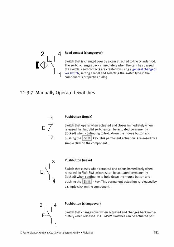
© Festo Didactic GmbH & Co. KG • Art Systems GmbH • FluidSIM 481
Reed contact (changeover)
Switch that is changed over by a cam attached to the cylinder rod. The switch changes back immediately when the cam has passed the switch. Reed contacts are created by using a general changeo-ver switch, setting a label and selecting the switch type in the component’s properties dialog.
21.3.7 Manually Operated Switches
Pushbutton (break)
Switch that opens when actuated and closes immediately when released. In FluidSIM switches can be actuated permanently (locked) when continuing to hold down the mouse button and
pushing the Shift key. This permanent actuation is released by a
simple click on the component.
Pushbutton (make)
Switch that closes when actuated and opens immediately when released. In FluidSIM switches can be actuated permanently (locked) when continuing to hold down the mouse button and
pushing the Shift - key. This permanent actuation is released by
a simple click on the component.
Pushbutton (changeover)
Switch that changes over when actuated and changes back imme-diately when released. In FluidSIM switches can be actuated per-

482 © Festo Didactic GmbH & Co. KG • Art Systems GmbH • FluidSIM
manently (locked) when continuing to hold down the mouse button
and pushing the Shift - key. This permanent actuation is released
by a simple click on the component.
Detent switch (break)
Switch that opens and locks when actuated.
Detent switch (make)
Switch that closes and locks when actuated.
Detent switch (changeover)
Switch that changes over and locks when actuated.
21.3.8 Pressure Switches
Pneumatic to electric converter
The converter produces an electrical signal, if the preset differential pressure of the differential pressure switch is exceeded.
Pressure switch (break)
Switch that opens when the preset switching pressure of the pneumatic or hydraulic pressure switch is exceeded. Pressure

© Festo Didactic GmbH & Co. KG • Art Systems GmbH • FluidSIM 483
switches are created by using a general break switch and setting a label.
Pressure switch (make)
The switch closes when the preset switching pressure of the pneu-matic or hydraulic pressure switch is exceeded. Pressure switches are created by using a general make switch and setting a label.
Pressure switch (changeover)
The switch changes over when the preset switching pressure of the pneumatic or hydraulic pressure switch is exceeded. Pressure switches are created by using a general changeover switch and setting a label.
Pressure switch
The switch relays an electrical signal when the preset switching pressure at the pneumatic pressure switch is exceeded.
Pressure switch
The switch relays an electrical signal when the preset switching pressure at the hydraulic pressure switch is exceeded.

484 © Festo Didactic GmbH & Co. KG • Art Systems GmbH • FluidSIM
21.3.9 Proximity Switches
Magnetic proximity switch
Switch that closes when a solenoid is brought nearby. In the Simu-lation Mode the proximity switch can also be actuated by clicking on it.
Inductive proximity switch
Switch that closes when the induced electro-magnetic field is changed. In the Simulation Mode the proximity switch can also be actuated by clicking on it.
Capacitive proximity switch
Switch that closes when its electrostatic field is changed. In the Simulation Mode the proximity switch can also be actuated by clicking on it.
Optical proximity switch
Switch that closes when the light barrier is interrupted. In the Simulation Mode the proximity switch can also be actuated by clicking on it.

© Festo Didactic GmbH & Co. KG • Art Systems GmbH • FluidSIM 485
21.3.10 Relay
Relay
The relay picks up immediately when current is supplied and drops out immediately when current is removed.
Adjustable parameters Resistance: 1 ... 10000 Ohm (550) Minimum voltage: 0.1 ... 300 V (20)
Relay with switch-on delay
The relay picks up after a preset time when current is supplied and drops out immediately when current is removed.
Adjustable parameters Delay time: 0 ... 999 s (5) Resistance: 1 ... 10000 Ohm (550) Minimum voltage: 0.1 ... 300 V (20)
Relay with switch-off delay
The relay picks up immediately when current is supplied and drops out after a preset time when current is removed.
Adjustable parameters Delay time: 0 ... 999 s (5) Resistance: 1 ... 10000 Ohm (550) Minimum voltage: 0.1 ... 300 V (20)

486 © Festo Didactic GmbH & Co. KG • Art Systems GmbH • FluidSIM
Relay counter
The relay picks up after a predefined number of current pulses has/have been counted between the connections A1 and A2. If a potential is supplied between the connections R1 and R2, the counter is reset to its predefined value. In the Simulation Mode the relay counter can also be reset by clicking on it.
Adjustable parameters Counter: 0 ... 9999 (5) Resistance: 1 ... 10000 Ohm (550) Minimum voltage: 0.1 ... 300 V (20)
Starting current limiter
The starting current limiter consists essentially of a relay, whose coil is situated between the connections IN and 0V, and whose switch contact is situated between the connections 24V and OUT. An electronic longitudinal controller restricts, with a switched relay contact, the current flow to the preset value for the specified dura-tion. The starting current limiter is usually deployed in combination with the electric motor.
Adjustable parameters Duration: 1 ... 10000 ms (0.05) Current limit: 0.01 ... 100 A (2)

© Festo Didactic GmbH & Co. KG • Art Systems GmbH • FluidSIM 487
21.3.11 Controller
Comparator
The comparator is a discontinuous (switching) two-step action controller with differential gap (hysteresis). When activated, it delivers a predefined voltage signal. The switch-on value for the activation is defined by nominal value + 1/2 hysteresis and the switch-off value by nominal value - 1/2 hysteresis. The comparator requires a power supply of 24 V.
Adjustable parameters Set value voltage: -300 ... 300 V (5) Hysteresis: 0 ... 100 V (0) Minimum voltage: 0.1 ... 300 V (13) Resistance: 1 ... 10000 Ohm (100)
PID controller
The PID-Controller is a continuous controller consisting of three control elements: Proportional, Integral and Derivative. The adjust-able parameters refer to the PID-Controller in the Technology Package TP111 pneumatic control TP511 hydraulic control from Festo Didactic. The output voltage restriction can be set within the range (i) -10 V to + 10 V or (ii) 0 V to +10 V. In the range (i), a ma-nipulated variable offset from -7 V to + 7 V can be specified, and in the range (ii) a manipulated variable offset from 1.5 V to 8.5 V can be specified. The PID-controller requires a power supply of 24 V.
Adjustable parameters Range selection: -10 .. 10 V,0 .. 10 V (-10 .. 10 V) Proportional gain: 0 ... 1000 (1) Integral gain: 0 ... 1000 1/s (0) Derivation gain: 0 ... 1000 ms (0) Control quantity offset: -7 ... 7 V (0)

488 © Festo Didactic GmbH & Co. KG • Art Systems GmbH • FluidSIM
Status controller
The status controller is especially suitable for controlling pneumatic positioning circuits. A pneumatic positioning circuit counts to the controlled systems that can only be unsatisfactorily controlled with a standard controller. Three parameters can be attributed to the present status controller: position, speed and acceleration of the piston. The controller is therefore referred to as a “triple loop” controller. Speed and acceleration are not measured with sensors out of cost reasons. They are calculated by the controller from the differences in position. The adjustable parameters refer to the status controller in the Technology Package TP111 Closed-loop pneumatics TP511 Closed-loop hydraulics from Festo Didactic. The output voltage restriction can be set within the range (i) -10 V to + 10 V or (ii) 0 V to +10 V. In the range (i), a manipulated variable offset from -7 V to + 7 V can be specified, and in the range (ii) a manipulated variable offset from 1.5 V to 8.5 V can be specified. The status controller requires a power supply of 24 V.
Adjustable parameters Range selection: -10 .. 10 V,0 .. 10 V (-10 .. 10 V) Deviation gain: 0 ... 10 (1) Velocity damping: 0 ... 100 ms (0) Acceleration damping: 0 ... 10 ms2 (0) Total gain: 0 ... 1000 (1) Control quantity offset: -7 ... 7 V (0)

© Festo Didactic GmbH & Co. KG • Art Systems GmbH • FluidSIM 489
21.3.12 EasyPort/OPC/DDE Components
FluidSIM Output Port
Communication with the EasyPort-Hardware and other applications is implemented with the FluidSIM-Output.
FluidSIM Input Port
Communication with the EasyPort-Hardware and other applications is implemented with the FluidSIM-Input.
FluidSIM Output Port (analog)
Communication with the EasyPort-Hardware and other applications is implemented with the analog FluidSIM-Output.
FluidSIM Input Port (analog)
Communication with the EasyPort-Hardware and other applications is implemented with the analog FluidSIM-Input.

490 © Festo Didactic GmbH & Co. KG • Art Systems GmbH • FluidSIM
Multi-pin plug distributor
Communication with EasyPort hardware, as well as with other applications, is carried out with the multi-pin plug distributor. The contacts on the right-hand side (1, 3, 5, 7, 9 and 11) represent the digital outputs, and the contacts on the left-hand side (0, 2, 4, 6, 8 and 10) the digital inputs. If the “Priority for connected hardware” switch is activated, only the input signals from the external sensors are taken into consideration, if an EasyPort has been connected.
Universal-I/O
The universal input/output-unit is connected with the multi-pin plug distributor by a label. The component is a input if the label refers to a input channel of the multi-pin plug distributor. The component is an output if the label refers to an output channel of the multi-pin plug distributor. If used as an input the universal I/O-component is a voltage source. If the correspondent input channel of the multi-pin plug distributor on high level, the universal I/O-Component delivers 24 V, otherwise 0V. If used as an output chan-nel, the universal I/O-component sets the correspondent output channel of the multi-pin plug distributor on high level, if there is a higher voltage than 20 V.

© Festo Didactic GmbH & Co. KG • Art Systems GmbH • FluidSIM 491
21.4 Electrical Components (American Standard)
21.4.1 Power Supply
Electrical connection 0V (ladder)
0V connection of the power supply.
Adjustable parameters Voltage: 0 ... 400 V (0)
Electrical connection 24V (ladder)
24V connection of the power supply.
Adjustable parameters Voltage: 0 ... 400 V (24)
21.4.2 General Switches
Break switch (ladder)
General break switch that is tailored depending on the type of component that actuates it. For example, if the break switch is

492 © Festo Didactic GmbH & Co. KG • Art Systems GmbH • FluidSIM
linked via a label to a switch-off delay relay, the break switch changes to a switch-off delay break switch in the circuit diagram.
Make switch (ladder)
General make switch that is tailored according to the component that actuates it. For example, if the make switch is linked via a label to a switch-on delayed relay, the make switch changes to a switch-on delayed make switch in the circuit diagram.
21.4.3 Delay Switches
Break switch (switch-on delayed, ladder)
Switch with delayed opening after pickup. Switch-on delayed break switches are created by using a general break switch and setting a label.
Make switch (switch-on delayed, ladder)
Switch with delayed closing after pickup. Switch-on delayed make switches are created by using a general make switch and setting a label.
Break switch (switch-off delayed, ladder)
Switch with delayed closing after dropout. Switch-off delayed break switches are created by using a general break switch and setting a label.

© Festo Didactic GmbH & Co. KG • Art Systems GmbH • FluidSIM 493
Make switch (switch-off delayed, ladder)
Switch with delayed opening after dropout. Switch-off delayed make switches are created by using a general make switch and setting a label.
21.4.4 Limit Switches
Limit switch (break, ladder)
Switch that is opened by a cam attached to the cylinder rod. The switch closes immediately when the cam has passed the switch. Limit switches are created by using a general break switch and setting a label.
Switch with roll (break, ladder)
Switch that is opened by a cam attached to the cylinder rod. The switch closes immediately when the cam has passed the switch. Limit switches are created by using a general break switch and setting a label.
Reed contact (break, ladder)
Switch that is opened by a cam attached to the cylinder rod. The switch closes immediately when the cam has passed the switch. Limit switches are created by using a general break switch and setting a label.

494 © Festo Didactic GmbH & Co. KG • Art Systems GmbH • FluidSIM
Limit switch (make, ladder)
Switch that is closed by a cam attached to the cylinder rod. The switch opens immediately when the cam has passed the switch. Limit switches are created by using a general make switch and setting a label.
Switch with roll (make, ladder)
Switch that is closed by a cam attached to the cylinder rod. The switch opens immediately when the cam has passed the switch. Limit switches are created by using a general make switch and setting a label.
Reed contact (make, ladder)
Switch that is closed by a cam attached to the cylinder rod. The switch opens immediately when the cam has passed the switch. Limit switches are created by using a general make switch and setting a label.
21.4.5 Manually Operated Switches
Pushbutton (break, ladder)
Switch that opens when actuated and closes immediately when released. In FluidSIM switches can be actuated permanently (locked) when continuing to hold down the mouse button and
pushing the Shift key. This permanent actuation is released by a
simple click on the component.

© Festo Didactic GmbH & Co. KG • Art Systems GmbH • FluidSIM 495
Pushbutton (make, ladder)
Switch that closes when actuated and opens immediately when released. In FluidSIM switches can be actuated permanently (locked) when continuing to hold down the mouse button and
pushing the Shift key. This permanent actuation is released by a
simple click on the component.
Pushbutton (changeover, ladder)
Switch that changes over when actuated and changes back imme-diately when released. In FluidSIM switches can be actuated per-manently (locked) when continuing to hold down the mouse button
and pushing the Shift key. This permanent actuation is released
by a simple click on the component.
21.4.6 Pressure Switches
Pressure switch (break, ladder)
Switch that opens when the preset switching pressure of the pneumatic or hydraulic pressure switch is exceeded. Pressure switches are created by using a general break switch and setting a label.
Pressure switch (make, ladder)
The switch closes when the preset switching pressure of the pneu-matic or hydraulic pressure switch is exceeded. Pressure switches are created by using a general make switch and setting a label.

496 © Festo Didactic GmbH & Co. KG • Art Systems GmbH • FluidSIM
21.4.7 Relays
Relay
The relay picks up immediately when current is supplied and drops out immediately when current is removed.
Adjustable parameters Resistance: 1 ... 10000 Ohm (550) Minimum voltage: 0.1 ... 300 V (20)
Relay with switch-on delay (ladder)
The relay picks up after a preset time when current is supplied and drops out immediately when current is removed.
Adjustable parameters Delay time: 0 ... 999 s (5) Resistance: 1 ... 10000 Ohm (550) Minimum voltage: 0.1 ... 300 V (20)
Relay with switch-off delay (ladder)
The relay picks up immediately when current is supplied and drops out after a preset time when current is removed.
Adjustable parameters Delay time: 0 ... 999 s (5) Resistance: 1 ... 10000 Ohm (550) Minimum voltage: 0.1 ... 300 V (20)

© Festo Didactic GmbH & Co. KG • Art Systems GmbH • FluidSIM 497
21.5 Electronic components
21.5.1 Power supply
Constant voltage source
A constant voltage source is an ideal voltage source, which can maintain a fixed voltage that does not depend on the output cur-rent or load resistance.
Adjustable parameters Voltage: 0 ... 400 V (12)
Potential
A potential is an ideal voltage source with a reference point of “ground”.
Adjustable parameters Voltage: -400 ... 400 V (5)
Ground
The ground symbol defines the 0 V reference potential for all signal and operating voltages.

498 © Festo Didactic GmbH & Co. KG • Art Systems GmbH • FluidSIM
Three-phase alternator
A three-phase alternator supplies a combined set of three sinusoi-dal alternating electric voltages. The voltages are phase shifted to one another.
There are three inductors inside the alternator, spatially off-set by 120°. The magnetic field of an evenly rotating permanent magnet induces three alternating voltages, phase shifted to one another by 120°.
Adjustable parameters Frequency: 0.01 ... 1000 Hz (50) String voltage: 0 ... 400 V (7)
Connector panel
Simple connector panel
DC power supply
Transformer for transforming alternating voltage into direct voltage.
Terminals 1 and 2 are used for connection to the alternating voltage source. The desired direct voltage is made available at terminals L+ and L-.
Adjustable parameters Effective (RMS) voltage (min): 10 ... 400 V (90) AC Frequency (min): 10 ... 100 Hz (30) Voltage (DC): 0 ... 400 V (12) Efficiency: 0.1 ... 1 (0.9)

© Festo Didactic GmbH & Co. KG • Art Systems GmbH • FluidSIM 499
DC power supply
Transformer for transforming alternating voltage into direct voltage.
Terminals 1 and 2 are used for connection to the alternating voltage source. The desired direct voltage is made available at terminals L+ and L-.
L1
Phase conductor which makes a sinusoidal alternating voltage available with adjustable amplitude, frequency and phase dis-placement. A phase displacement of 0° is preset as a default value for L1.
Adjustable parameters Effective (RMS) voltage: 0 ... 400 V (230) Frequency: 1 ... 100 Hz (50) Phase shift: 0 ... 360 deg (0)
L2
Phase conductor which makes a sinusoidal alternating voltage available with adjustable amplitude, frequency and phase dis-placement. A phase displacement of 120° is preset as a default value for L2.
Adjustable parameters Effective (RMS) voltage: 0 ... 400 V (230) Frequency: 1 ... 100 Hz (50) Phase shift: 0 ... 360 deg (120)

500 © Festo Didactic GmbH & Co. KG • Art Systems GmbH • FluidSIM
L3
Phase conductor which makes a sinusoidal alternating voltage available with adjustable amplitude, frequency and phase dis-placement. A phase displacement of 240° is preset as a default value for L3.
Adjustable parameters Effective (RMS) voltage: 0 ... 400 V (230) Frequency: 1 ... 100 Hz (50) Phase shift: 0 ... 360 deg (240)
N
Neutral conductor
PE
Protective earth conductor
21.5.2 Passive components
Resistor
A resistor represents an ideal ohmic resistor.
Adjustable parameters Resistance: 1e-6 ... 1E8 Ohm (100)

© Festo Didactic GmbH & Co. KG • Art Systems GmbH • FluidSIM 501
Resistor, temperature-dependent (NTC)
In a temperature-dependent resistor of type NTC, the resistance value falls as the temperature rises.
Adjustable parameters Reference Resistance: 1 ... 1E6 Ohm (5208) Reference temperature: 0 ... 100 °C (23)
Resistor, voltage-dependent (varistor, VDR)
A varistor is a voltage-dependent resistor. Resistance decreases abruptly once a particular voltage threshold is exceeded.
Resistor, light-dependent (LDR)
A light-dependent resistor consists of an amorphous semiconduc-tor film. As the incidence of light is increased, electrical resistance is decreased, due to the internal photoelectric effect.
Adjustable parameters Light intensity: 0 ... 100 % (50) Min. Resistance: 1 ... 1E6 Ohm (183) Max. Resistance: 1 ... 1E6 Ohm (34324)
Potentiometer
A potentiometer is an electrical resistance component with me-chanically adjustable (by means of rotation or sliding) resistance values. It provides three connectors and is mainly used as a contin-uously adjustable voltage divider.

502 © Festo Didactic GmbH & Co. KG • Art Systems GmbH • FluidSIM
Adjustable parameters Potentiometer position: 0 ... 100 % (0) Resistance: 1E-4 ... 100000 kOhm (1)
Capacitor
A capacitor is a passive electrical component which is able to store electric charge (and therefore electric energy.)
The capacitor in its basic configuration consists of two electrically conductive surfaces, the electrodes. The electrodes are separated through an insulating material, the so-called dielectric. The separa-tion of the two electrodes is so narrow, that the electrical forces are able to act through the insulating material.
If a constant voltage is applied to the connectors of an uncharged capacitor, a current flows for a short period of time and one of the electrodes is positively charged, the other one negatively. This electric charge is retained when the capacitor is disconnected from the voltage source. If charge resp. electric flow is extracted from the capacitor, its voltage drops again.
Adjustable parameters Capacity: 1E-4 ... 1E7 uF (1)
Capacitor, polarized
A capacitor is a passive electrical component which is able to store electric charge (and therefore electric energy.)
The capacitor in its basic configuration consists of two electrically conductive surfaces, the electrodes. The electrodes are separated through an insulating material, the so-called dielectric. The separa-tion of the two electrodes is so narrow, that the electrical forces are able to act through the insulating material.

© Festo Didactic GmbH & Co. KG • Art Systems GmbH • FluidSIM 503
If a constant voltage is applied to the connectors of an uncharged capacitor, a current flows for a short period of time and one of the electrodes is positively charged, the other one negatively. This electric charge is retained when the capacitor is disconnected from the voltage source. If charge resp. electric flow is extracted from the capacitor, its voltage drops again.
In contrast to the non-polarized capacitor, the polarized capacitor is only suitable for DC and for AC voltage that does not reverse the capacitor’s polarity. The advantage of the polarized capacitor is the much higher capacity for the same form factor compared to non-polarized capacitors.
Adjustable parameters Capacity: 1E-4 ... 1E7 uF (1)
Inductor
An inductor is a passive electrical component which is able to create induction voltage.
An inductor, also called an inductance, in its basic configuration consists of wire coils. The inductor provides two terminals.
If an inductor is connected to a DC voltage, then an exponentially increasing current will flow.
Adjustable parameters Inductance: 1E-3 ... 1E4 mH (100)
Transformer
The transformer consists of two transformer coils. If an alternating voltage is applied to one transformer coil, an alternating voltage is induced in the second coil. In the no-load case, the value of the new voltage when compared to the originally supplied voltage, follows

504 © Festo Didactic GmbH & Co. KG • Art Systems GmbH • FluidSIM
the ratio of the number of windings of the corresponding coils to each other.
Adjustable parameters Inductance 1: 1E-3 ... 1E4 mH (595) Inductance 2: 1E-3 ... 1E4 mH (66) Coupling coefficient: 0 ... 1 (1)
21.5.3 Semiconductor
Diode
A diode allows an electric current to pass in only one direction, while in the opposite direction it acts as an insulator. Therefore, diodes have a forward direction and a reverse direction.
Adjustable parameters Reference voltage: 0.1 ... 100 V (0.7) Reference current: 1 ... 1000 mA (12.6) Resistance in series: 0.001 ... 1000 Ohm (0.0341512) Saturation current: 1e-15 ... 100 A (7.02767e-9)
Light-emitting diode, LED (red)
A light-emitting diode (LED) is a semiconductor component that emits light and has the electrical characteristics of a diode. If an electric current is flowing through the diode in forward direction, it emits light with a wavelength that depends on the semiconductor material and doping.

© Festo Didactic GmbH & Co. KG • Art Systems GmbH • FluidSIM 505
To make the use of the LED as a simple signal indicator easier, FluidSIM allows setting the color independent of the physical characteristics.
Adjustable parameters Reference voltage: 0.1 ... 100 V (2) Reference current: 1 ... 1000 mA (25) Resistance in series : 0.001 ... 1000 Ohm (12.5) Saturation current: 1e-15 ... 100 A (1e-12)
Light-emitting diode, LED (green)
A light-emitting diode (LED) is a semiconductor component that emits light and has the electrical characteristics of a diode. If an electric current is flowing through the diode in forward direction, it emits light with a wavelength that depends on the semiconductor material and doping.
To make the use of the LED as a simple signal indicator easier, FluidSIM allows setting the color independent of the physical characteristics.
Adjustable parameters Reference voltage: 0.1 ... 100 V (2.2) Reference current: 1 ... 1000 mA (30) Resistance in series : 0.001 ... 1000 Ohm (12.5) Saturation current: 1e-15 ... 100 A (1e-12)
Light-emitting diode, LED (blue)
A light-emitting diode (LED) is a semiconductor component that emits light and has the electrical characteristics of a diode. If an electric current is flowing through the diode in forward direction, it emits light with a wavelength that depends on the semiconductor material and doping.

506 © Festo Didactic GmbH & Co. KG • Art Systems GmbH • FluidSIM
To make the use of the LED as a simple signal indicator easier, FluidSIM allows setting the color independent of the physical characteristics.
Adjustable parameters Reference voltage: 0.1 ... 100 V (4) Reference current: 1 ... 1000 mA (35) Resistance in series : 0.001 ... 1000 Ohm (12.5) Saturation current: 1e-15 ... 100 A (1e-12)
Light-emitting diode, LED (green/red)
A light-emitting diode (LED) is a semiconductor component that emits light and has the electrical characteristics of a diode. If an electric current is flowing through the diode in forward direction, it emits light with a wavelength that depends on the semiconductor material and doping.
In this component, a green and a red LED with opposite polarity are connected in parallel. Depending on the current direction either the green or red LED lights up. Connected to alternating current with a frequency higher than about 30 Hz, the human eye cannot recog-nize the blinking and it seems as if both LEDs are lit simultaneously.
Adjustable parameters Reference voltage: 0.1 ... 100 V (2) Reference current: 1 ... 1000 mA (25) Resistance in series : 0.001 ... 1000 Ohm (12.5) Saturation current: 1e-15 ... 100 A (1e-12)
Zener diode
Because of their characteristics, zener diodes are used in numerous circuitries for stabilizing and limiting electrical voltages. In forward direction, they behave like normal diodes. In reverse direction, resistance drops off considerably after the voltage exceeds a cer-

© Festo Didactic GmbH & Co. KG • Art Systems GmbH • FluidSIM 507
tain value, the so-called breakdown voltage. The voltage does not increase by much after that, even if the electric current is increased.
Adjustable parameters Reference voltage: 0.1 ... 100 V (0.7) Reference current: 1 ... 10000 mA (9) Saturation current: 1e-10 ... 100 A (1e-10) Z-voltage: 0.1 ... 100 V (10) Current at Z-voltage: 1 ... 10000 mA (15)
NPN transistor
An NPN transistor is a bipolar junction transistor (BJT). It is operat-ed with an electric current and is used for switching and amplifying signals without using mechanically moving parts.
There are two types of BJTs: NPN and PNP. The letters indicate the order and doping type of the layers. Essentially, a BJT constitutes two p-n junctions connected together in series (like that of a p-n diode.) The three terminals are called collector (C), base (B) and emitter (E).
Adjustable parameters Forward current gain: 0.1 ... 1000 (120) Reverse current gain: 0.1 ... 1000 (1) Saturation current: 1e-16 ... 1e-3 A (8.81138e-14) Forward early voltage: 1 ... 1000 V (64)
PNP transistor
An PNP transistor is a bipolar junction transistor (BJT). It is operated with an electric current and is used for switching and amplifying signals without using mechanically moving parts.
There are two types of BJTs: NPN and PNP. The letters indicate the order and doping type of the layers. Essentially, a BJT constitutes two p-n junctions connected together in series (like that of a p-n

508 © Festo Didactic GmbH & Co. KG • Art Systems GmbH • FluidSIM
diode.) The three terminals are called collector (C), base (B) and emitter (E).
Adjustable parameters Forward current gain: 0.1 ... 1000 (230) Reverse current gain: 0.1 ... 1000 (1) Saturation current: 1e-16 ... 1e-3 A (8.81138e-14) Forward early voltage: 1 ... 1000 V (64)
N-channel JFET
A junction gate field-effect transistor (JFET) controls the electrical current that flows through the channel between the source and drain terminals, by using a junction between the gate connector and the channel.
Depending on doping type, JFETs are classified in two types: n-channel and p-channel JFETs.
Adjustable parameters Threshold voltage: -20 ... 0 V (-3) Transconductance parameter: 1e-6 ... 1e-1 A/V2 (1.304e-3) Channel-length modulation parameter: 1e-6 ... 1e-1 1/V (2.25e-3)
P-channel JFET
A junction gate field-effect transistor (JFET) controls the electrical current that flows through the channel between the source and drain terminals, by using a junction between the gate terminal and the channel.
Depending on doping type, JFETs are classified in two types: n-channel and p-channel JFETs.
Adjustable parameters Threshold voltage: 0 ... 20 V (2.5) Transconductance parameter: 1e-6 ... 1e-1 A/V2 (1.271e-3)

© Festo Didactic GmbH & Co. KG • Art Systems GmbH • FluidSIM 509
Channel-length modulation parameter: 1e-6 ... 1e-1 1/V (0.04)
N-channel MOSFET-Transistor
A metal-oxide-semiconductor field-effect transistor (MOSFET) is an active component with at least three terminals (electrodes): G (gate), D (drain) and S (source.) In some designs, an additional B (bulk) terminal is fed to the outside. Usually though, B is connected internally with S.
Like other field-effect transistors, a MOSFET acts as a voltage-controlled resistor, meaning that the voltage between gate and source can be used to change the resistance (and thus the electri-cal current) between drain and source by several orders of magni-tude.
Depending on doping type, MOSFETs are classified in two types: n-channel and p-channel MOSFETs.
P-channel MOSFET
A metal-oxide-semiconductor field-effect transistor (MOSFET) is an active component with at least three terminals (electrodes): G (gate), D (drain) and S (source.) In some designs, an additional B (bulk) terminal is fed to the outside. Usually though, B is connected internally with S.
Like other field-effect transistors, a MOSFET acts as a voltage-controlled resistor, meaning that the voltage between gate and source can be used to change the resistance (and thus the electri-cal current) between drain and source by several orders of magni-tude.
Depending on doping type, MOSFETs are classified in two types: n-channel and p-channel MOSFETs.

510 © Festo Didactic GmbH & Co. KG • Art Systems GmbH • FluidSIM
Unijunction transistor
Similar to a normal bipolar transistor, a unijunction transistor (UJT) provides three terminals. Unlike a bipolar transistor however, but similar to a diode, there is only one p-n junction. In practice, it acts like a controlled diode that, despite the constant polarity of the applied voltage, can be made conductive or non-conductive. Be-cause of the two B terminals, the UJT is also called “double-base diode.”
If a small, positive control voltage against B1 is applied to the emitter, nothing happens at first. If the control voltage is raised further and a certain potential is reached, the UEB1 voltage will collapse abruptly, and at the same time the emitter current will jump to a certain value. In a sense, the UJT “has been fired.” This behavior is very similar to a thyristor. A UJT is cleared when the emitter current falls below a certain threshold.
Thyristor
A thyristor is a semiconductor component built from four or more semiconductor films of varying levels of doping. Thyristors are switchable components, meaning they are non-conductive in their initial state and can be switched on through a small gate current. After a thyristor has been switched on, it remains conductive even if there is no gate current. A thyristor can be switched off by falling below a minimum current, the so-called holding current.
DIAC
A DIAC (diode for alternating current) is an electronic component with only two terminals. DIACs are also referred to as “symmetrical trigger diodes.” The junction between the terminals only becomes conductive after a breakover voltage has been reached.
The DIAC’s bidirectional layout allows for the switching of alternat-ing voltages. As soon as the voltage on the terminals (A1 and A2)

© Festo Didactic GmbH & Co. KG • Art Systems GmbH • FluidSIM 511
rises above a certain threshold voltage, it will switch through and the p-n junction becomes conductive. Resistance will rise rapidly again after the current that is flowing through the DIAC falls below a certain value (the holding current.) This procedure is referred to as “resetting the DIAC.”
TRIAC
In principle, A TRIAC (triode for alternating current) represents an inverse-parallel connection of two thyristors. This allows for switch-ing of alternating current, while a single thyristor can switch in only one direction and thus acts - in its on-state - like a diode.
A TRIAC has a control terminal G (gate) and two main terminals MT1 and MT2, where MT2 is usually directly connected to the casing. In order to be able to use a single control terminal for both thyristors, TRIACs contain two firing, or helper, thyristor junctions, so that it can be flipped into the low-impedance state by using a positive and negative control pulse.
21.5.4 Measuring instruments / Sensors
Ohmmeter
An ohmmeter is an electrical test instrument which is used to measure the electrical resistance of components.
Adjustable parameters Voltage: 0.1 ... 9 V (9) Series resistor: 1 ... 1000 kOhm (47)

512 © Festo Didactic GmbH & Co. KG • Art Systems GmbH • FluidSIM
Oscilloscope
An oscilloscope is an electronic test instrument that allows visual observation of one or more electrical voltages and their change over time on a display device. The oscilloscope displays a history graph, usually as a two-dimensional graph, where the horizontal x-axis represents time and the vertical y-axis the voltages that are to be displayed. The resulting image is called an oscillogram.
Adjustable parameters Resistance: 1E-3 ... 10 MOhm (10)
Power factor meter
Effective power factor is measured in AC circuits with the power factor meter. The measuring instrument is equipped with a current path (terminals 1 and 3) and a voltage path (terminals 4 and 2). Connect the measuring instrument’s current path like an ammeter and the voltage path like a voltmeter.
Adjustable parameters Time interval: 0.001 ... 100 s (0.1)
Wattmeter
The wattmeter is used to measure effective power in electric cir-cuits. It’s equipped with a current path (terminals 1 and 3) and a voltage path (terminals 4 and 2). The wattmeter multiplies meas-ured values for voltage and current with each other and displays the result. Connect the measuring instrument’s current path like an ammeter and the voltage path like a voltmeter.
Apparent power, reactive power and power factor can be measured with this wattmeter in addition to effective power.

© Festo Didactic GmbH & Co. KG • Art Systems GmbH • FluidSIM 513
Adjustable parameters Time interval: 0.001 ... 100 s (0.1)
21.5.5 Switches
Circuit breaker
Circuit breakers protect connected circuits from overloading. They’re equipped with a thermal trigger and an electromagnetic trigger. The thermal trigger is usually a bimetallic switch which is tripped after a specified period of time when current flowing through the circuit breaker is greater than nominal current. In the event of a short-circuit or excessive overcurrent, the electromagnet-ic trigger is tripped and the circuit break opens very quickly. The circuit breaker is equipped with trip-free release, which means that it opens even if it’s held closed manually. The switch’s character-istic can be selected under the circuit breaker’s attributes. If char-acteristic B is selected, the electromagnetic trigger is tripped at an amperage of 3 times nominal current, or at 5 times nominal current if characteristic C is selected. For thermal triggering, a selected tripping point can be specified for a given overcurrent value.
The symbol for the circuit breaker shows the switch in its open state. The circuit breaker is closed automatically when simulation in FluidSIM is started, so that it doesn’t have to be closed manually for each simulation.
Adjustable parameters Rated current: 0.1 ... 100 A (10) Tripping characteristic: B,C (B) Tripping temperature: 50 ... 150 °C (80) Multiple of nominal current: 1.5 ... 10 (2) Tripping time: 0.1 ... 100 s (30)

514 © Festo Didactic GmbH & Co. KG • Art Systems GmbH • FluidSIM
3-pole circuit breaker
Circuit breakers protect connected circuits from overloading. They’re equipped with a thermal trigger and an electromagnetic trigger. The thermal trigger is usually a bimetallic switch which is tripped after a specified period of time when current flowing through the circuit breaker is greater than nominal current. In the event of a short-circuit or excessive overcurrent, the electromagnet-ic trigger is tripped and the circuit break opens very quickly. The circuit breaker is equipped with trip-free release, which means that it opens even if it’s held closed manually.
In the case of this 3-phase circuit breaker, each phase is monitored separately. If overloading occurs in any single phase, all three phases are interrupted. The switch’s characteristic can be se-lected under the circuit breaker’s attributes. If characteristic B is selected, the electromagnetic trigger is tripped at an amperage of 3 times nominal current, or at 5 times nominal current if characteris-tic C is selected. For thermal triggering, a selected tripping point can be specified for a given overcurrent value.
The symbol for the circuit breaker shows the switch in its open state. The circuit breaker is closed automatically when simulation in FluidSIM is started, so that it doesn’t have to be closed manually for each simulation.
Adjustable parameters Rated current: 0.1 ... 100 A (10) Tripping characteristic: B,C (B) Tripping temperature: 50 ... 150 °C (80) Multiple of nominal current: 1.5 ... 10 (2) Tripping time: 0.1 ... 100 s (30)
Motor circuit breaker
Motor circuit breaker are used to protect connected motors against overloading. They’re equipped with a thermal trigger for minimal overcurrent and an electromagnetic trigger for short-circuits. This

© Festo Didactic GmbH & Co. KG • Art Systems GmbH • FluidSIM 515
motor circuit breaker has a 10 A tripping class. The thermal trigger starts to trip as of an amperage of 1.2 times nominal current and the electromagnetic trigger is tripped as of 7.2 times nominal current. If overloading occurs in any single phase, all three phases are interrupted when the circuit breaker is tripped. The circuit breaker has to be closed manually after tripping.
The symbol for the motor circuit breaker shows the switch in its open state. The circuit breaker is closed automatically when simu-lation in FluidSIM is started, so that it doesn’t have to be closed manually for each simulation.
Adjustable parameters Rated current: 0.1 ... 100 A (3) Tripping temperature: 50 ... 150 °C (80)
Motor protection relay
Motor protection relays are used to protect connected motors against overloading. If overloading occurs in any of the three con-nected phases, a connected switch can be actuated by means of the motor protection relay. In the event of overloading, power supply to the motor is usually interrupted via the its control circuit.
Adjustable parameters Rated current: 0.1 ... 100 A (1) Tripping temperature: 50 ... 150 °C (80)
PNOZ safety relay
Safety switching devices are essential constituents of safety tech-nology. This safety relay with positively driven contacts is used for the implementation of safety functions such as emergency stop or the monitoring of safety doors.
This type of safety relay is based on the safety switching device for the emergency stop function and the safety door in Festo Didactic’s

516 © Festo Didactic GmbH & Co. KG • Art Systems GmbH • FluidSIM
equipment set TP 250, “Safety in pneumatic systems”. The PNOZ S4 safety relay from Pilz is used in the equipment set. Correct wiring of the safety switching device is described in the operating instructions included with the PNOZ S4.
Adjustable parameters Operating mode: Automatic/Manual start,Monitored reset with falling edge,Monitored reset with rising edge (Automatic/Manual start) Min. Voltage: 0.1 ... 100 V (21.6)
21.5.6 Machines
Capacitor motor
The capacitor motor is a machine for converting electrical energy into mechanical energy (rotary motion). Capacitor motors are single-phase AC motors with squirrel-cage rotor. The rotary field in the stator is generated with the help of an additional capacitor, from which the name “capacitor motor” originates. In order to improve starting torque, a starter capacitor is used in addition to the operating capacitor. The capacitance of the starter and operat-ing capacitors can be adjusted, and direction of rotation can be selected. The Revolution (Switch) parameter indicates as of which speed switching from the starter capacitor to the operating capaci-tor takes place.
Terminal 1 and 2 are used to connected the alternating current required to operate the motor. Terminal 3 is a rotary terminal mechanism. A motor test bench or a further motor can be connect-ed here, for example. (The direction of rotation is usually reversed via the connection. This can be selected with the connecting cable.)

© Festo Didactic GmbH & Co. KG • Art Systems GmbH • FluidSIM 517
The capacitor motor’s characteristic data (for example winding resistances, inductances, number of pole pairs etc.) are automati-cally ascertained in the background after entering the performance data. Details can be found in the following separate section: Simu-lation of rotating machines.
Adjustable parameters Power: 0.001 ... 100 kW (0.25) Revolution: 1 ... 30000 1/min (1400) Voltage: 1 ... 10000 V (230) Frequency: 30 ... 100 Hz (50) Current: 0.1 ... 100 A (1.86) Capacity (Starting capacitor): 0.1 ... 100 uF (25) Capacity (Running capacitor): 0.1 ... 100 uF (10) Direction of rotation: Left,Right (Right) External torque: 0 ... 100 N.m (0) Revolution (Switch): 1 ... 100000 1/min (1000)
Capacitor motor
The capacitor motor is a machine for converting electrical energy into mechanical energy (rotary motion). Capacitor motors are single-phase AC motors with squirrel-cage rotor. The rotary field in the stator is generated with the help of an additional capacitor, from which the name “capacitor motor” originates. In order to improve starting torque, a starter capacitor is used in addition to the operating capacitor. The capacitance of the starter and operat-ing capacitors can be adjusted, and direction of rotation can be selected. The Revolution (Switch) parameter indicates as of which speed switching from the starter capacitor to the operating capaci-tor takes place.
The exploded view of the motor makes it possible to manually wire the stator coils and the capacitors to operating voltage.
Terminals 1 and 2 make reference to the operating capacitor. Ter-minals 3 and 4 make reference to the starter capacitor including a centrifugal switch, which opens when a specified speed is exceed-ed (parameter: Revolution (Switch)). Terminal 5 is a rotary terminal mechanism. A motor test bench or a further motor can be connect-

518 © Festo Didactic GmbH & Co. KG • Art Systems GmbH • FluidSIM
ed here, for example. (The direction of rotation is usually reversed via the connection. This can be selected with the connecting cable.)
The capacitor motor’s characteristic data (for example winding resistances, inductances, number of pole pairs etc.) are automati-cally ascertained in the background after entering the performance data. Details can be found in the following separate section: Simu-lation of rotating machines.
Adjustable parameters Power: 0.001 ... 100 kW (0.25) Revolution: 1 ... 30000 1/min (1400) Voltage: 1 ... 10000 V (230) Frequency: 30 ... 100 Hz (50) Current: 0.1 ... 100 A (1.86) Capacity (Starting capacitor): 0.1 ... 100 uF (25) Capacity (Running capacitor): 0.1 ... 100 uF (10) External torque: 0 ... 100 N.m (0) Revolution (Switch): 1 ... 100000 1/min (1000)
3-phase squirrel-cage asynchronous motor
The 3-phase asynchronous motor is a machine for converting electrical energy into mechanical energy (rotary motion). It’s a widely used type of induction motor which is simple, rugged and maintenance-free. It uses a short-circuited rotor and rotor current is generated by means of induction. Asynchronous motors are used in particular as high-performance servo-drives. The stator includes three windings, each of which is arranged at an angle 120° to the next. A slotted, laminated rotor core is used. A cage made of die-cast aluminum is inserted into the slots. The cage thus comprises a system of short-circuited electrical conductors.
The three phases of the 3-phase current are connected to terminal 1 through 3. Terminal 4 is a rotary terminal mechanism. A motor test bench or a further motor can be connected here, for example. (The direction of rotation is usually reversed via the connection. This can be selected with the connecting cable.)

© Festo Didactic GmbH & Co. KG • Art Systems GmbH • FluidSIM 519
The inner wiring selected in the parameters determines how en-tered machine performance data is interpreted in order to ascertain the machine’s characteristics data such as winding resistances, inductances, number of pole pairs etc. These characteristic ma-chine data are ascertained automatically in the background after the performance data have been entered. Details can be found in the following separate section: Simulation of rotating machines. In addition to the performance data, tightening torque and pull-out torque can also be entered to the parameters as a ratio to nominal torque. This makes it possible to specify the characteristic load curve of an actual machine somewhat more accurately.
Adjustable parameters Internal wiring: Star connection,Delta connection (Star connec-tion) Power: 0.001 ... 1000 kW (0.25) Revolution: 1 ... 10000 1/min (1350) Power factor cos φ: 0.1 ... 0.99 (0.78) Line-to-line voltage: 1 ... 10000 V (400) Phase current: 0.1 ... 100 A (0.77) Frequency: 30 ... 100 Hz (50) T_0 : T_N: 0.1 ... 10 (1.35) T_B : T_N: 0.1 ... 10 (1.58) External torque: 0 ... 100 N.m (0)
3-phase squirrel-cage asynchronous motor
The 3-phase asynchronous motor is a machine for converting electrical energy into mechanical energy (rotary motion). It’s a widely used type of induction motor which is simple, rugged and maintenance-free. It uses a short-circuited rotor and rotor current is generated by means of induction. Asynchronous motors are used in particular as high-performance servo-drives. The stator includes three windings, each of which is arranged at an angle 120° to the next. A slotted, laminated rotor core is used. A cage made of die-cast aluminum is inserted into the slots. The cage thus comprises a system of short-circuited electrical conductors.
The three phases of the 3-phase current are connected to terminal 1 through 3. Terminal 4 is a rotary terminal mechanism. A motor

520 © Festo Didactic GmbH & Co. KG • Art Systems GmbH • FluidSIM
test bench or a further motor can be connected here, for example. (The direction of rotation is usually reversed via the connection. This can be selected with the connecting cable.) The other electrical terminals are used for connection to the electrical section of the motor test bench.
The inner wiring selected in the parameters determines how en-tered machine performance data is interpreted in order to ascertain the machine’s characteristics data such as winding resistances, inductances, number of pole pairs etc. These characteristic ma-chine data are ascertained automatically in the background after the performance data have been entered. Details can be found in the following separate section: Simulation of rotating machines. In addition to the performance data, tightening torque and pull-out torque can also be entered to the parameters as a ratio to nominal torque. This makes it possible to specify the characteristic load curve of an actual machine somewhat more accurately.
Adjustable parameters Internal wiring: Star connection,Delta connection (Star connec-tion) Power: 0.001 ... 1000 kW (0.25) Revolution: 1 ... 10000 1/min (1350) Power factor cos φ: 0.1 ... 0.99 (0.78) Line-to-line voltage: 1 ... 10000 V (400) Phase current: 0.1 ... 100 A (0.77) Frequency: 30 ... 100 Hz (50) T_0 : T_N: 0.1 ... 10 (1.35) T_B : T_N: 0.1 ... 10 (1.58) External torque: -0 ... 100 N.m (0)
3-phase squirrel-cage asynchronous motor
The 3-phase asynchronous motor is a machine for converting electrical energy into mechanical energy (rotary motion). It’s a widely used type of induction motor which is simple, rugged and maintenance-free. It uses a short-circuited rotor and rotor current is generated by means of induction. Asynchronous motors are used in particular as high-performance servo-drives. The stator includes three windings, each of which is arranged at an angle 120° to the

© Festo Didactic GmbH & Co. KG • Art Systems GmbH • FluidSIM 521
next. A slotted, laminated rotor core is used. A cage made of die-cast aluminum is inserted into the slots. The cage thus comprises a system of short-circuited electrical conductors.
In this representation of the 3-phase motor, the terminals for the stator windings (U1-U2, V1-V2, W1-W2) are led to the outside. In this way, the desired wiring of the windings with star or delta con-nection can be completed from the outside. Terminal 1 is a rotary terminal mechanism. A motor test bench or a further motor can be connected here, for example. (The direction of rotation is usually reversed via the connection. This can be selected with the connect-ing cable.)
The inner wiring selected in the parameters determines how en-tered machine performance data is interpreted in order to ascertain the machine’s characteristics data such as winding resistances, inductances, number of pole pairs etc. These characteristic ma-chine data are ascertained automatically in the background after the performance data have been entered. Details can be found in the following separate section: Simulation of rotating machines. In addition to the performance data, tightening torque and pull-out torque can also be entered to the parameters as a ratio to nominal torque. This makes it possible to specify the characteristic load curve of an actual machine somewhat more accurately.
Adjustable parameters Internal wiring: Star connection,Delta connection (Star connec-tion) Power: 0.001 ... 1000 kW (0.25) Revolution: 1 ... 10000 1/min (1350) Power factor cos φ: 0.1 ... 0.99 (0.78) Line-to-line voltage: 1 ... 10000 V (400) Phase current: 0.1 ... 100 A (0.77) Frequency: 30 ... 100 Hz (50) T_0 : T_N: 0.1 ... 10 (1.35) T_B : T_N: 0.1 ... 10 (1.58) External torque: 0 ... 100 N.m (0)

522 © Festo Didactic GmbH & Co. KG • Art Systems GmbH • FluidSIM
3-phase squirrel-cage asynchronous motor
The 3-phase asynchronous motor is a machine for converting electrical energy into mechanical energy (rotary motion). It’s a widely used type of induction motor which is simple, rugged and maintenance-free. It uses a short-circuited rotor and rotor current is generated by means of induction. Asynchronous motors are used in particular as high-performance servo-drives. The stator includes three windings, each of which is arranged at an angle 120° to the next. A slotted, laminated rotor core is used. A cage made of die-cast aluminum is inserted into the slots. The cage thus comprises a system of short-circuited electrical conductors.
The three phases of the 3-phase current are connected to terminal 1 through 3. Terminal 4 is a rotary terminal mechanism. A motor test bench or a further motor can be connected here, for example. (The direction of rotation is usually reversed via the connection. This can be selected with the connecting cable.)
The inner wiring selected in the parameters determines how en-tered machine performance data is interpreted in order to ascertain the machine’s characteristics data such as winding resistances, inductances, number of pole pairs etc. These characteristic ma-chine data are ascertained automatically in the background after the performance data have been entered. Details can be found in the following separate section: Simulation of rotating machines. In addition to the performance data, tightening torque and pull-out torque can also be entered to the parameters as a ratio to nominal torque. This makes it possible to specify the characteristic load curve of an actual machine somewhat more accurately.
Adjustable parameters Internal wiring: Star connection,Delta connection (Star connec-tion) Power: 0.001 ... 1000 kW (0.25) Revolution: 1 ... 10000 1/min (1350) Power factor cos φ: 0.1 ... 0.99 (0.78) Line-to-line voltage: 1 ... 10000 V (400) Phase current: 0.1 ... 100 A (0.77) Frequency: 30 ... 100 Hz (50) T_0 : T_N: 0.1 ... 10 (1.35)

© Festo Didactic GmbH & Co. KG • Art Systems GmbH • FluidSIM 523
T_B : T_N: 0.1 ... 10 (1.58) External torque: 0 ... 100 N.m (0)
Synchronous motor
The synchronous motor is a machine for converting electrical ener-gy into mechanical energy (rotary motion). It’s a 3-phase motor in which the rotor always runs synchronous to the stator’s rotary field. This version of the synchronous motor is equipped with an addi-tional squirrel cage, so that it can be started up in accordance with the asynchronous motor principle.
Terminals 1 through 3 are used to connect 3-phase current for the generation of a rotary field in the motor’s stator. Terminals 5 and 6 are used to connect direct current to the excitation windings. Ter-minal 4 is a rotary terminal mechanism. A motor test bench or a further motor can be connected here, for example. (The direction of rotation is usually reversed via the connection. This can be selected with the connecting cable.)
If the synchronous motor is idled without a load, a so-called V curve can be recorded which reflects the relationship between excitation current and effective stator current. Nominal excitation current indicates the point of minimum stator current, at which power factor is also equal to 1.
Nominal excitation current can be specified as a ratio to maximum excitation current with the parameter Ratio Current : Max. Current. The absolute value of nominal excitation current is determined by multiplying maximum excitation current by the specified ratio (e.g. maximum excitation current 0.95 A * 0.5 = nominal excitation current 0.475 A).
The synchronous motor’s characteristic data (for example winding resistances, inductances, number of pole pairs etc.) are automati-cally ascertained in the background after entering the performance data. Details can be found in the following separate section: Simu-lation of rotating machines.
Adjustable parameters

524 © Festo Didactic GmbH & Co. KG • Art Systems GmbH • FluidSIM
Power: 0.001 ... 1000 kW (0.3) Revolution: 1 ... 10000 1/min (1500) Power factor cos φ: 0.1 ... 1 (0.97) Line-to-line voltage: 1 ... 10000 V (400) Phase current: 0.1 ... 100 A (0.66) Frequency: 30 ... 100 Hz (50) Voltage (Exciter, Max.): 1 ... 10000 V (150) Current (Exciter, Max.): 0.1 ... 100 A (0.95) I_f : I_f_max: 0.01 ... 1 (0.5) External torque: 0 ... 100 N.m (0)
Synchronous motor
The synchronous motor is a machine for converting electrical ener-gy into mechanical energy (rotary motion). It’s a 3-phase motor in which the rotor always runs synchronous to the stator’s rotary field. This version of the synchronous motor is equipped with an addi-tional squirrel cage, so that it can be started up in accordance with the asynchronous motor principle.
Terminals 1 through 3 are used to connect 3-phase current for the generation of a rotary field in the motor’s stator. Terminals 5 and 6 are used to connect direct current to the excitation windings. Ter-minal 4 is a rotary terminal mechanism. A motor test bench or a further motor can be connected here, for example. (The direction of rotation is usually reversed via the connection. This can be selected with the connecting cable.) The other electrical terminals are used for connection to the electrical section of the motor test bench.
If the synchronous motor is idled without a load, a so-called V curve can be recorded which reflects the relationship between excitation current and effective stator current. Nominal excitation current indicates the point of minimum stator current, at which power factor is also equal to 1.
Nominal excitation current can be specified as a ratio to maximum excitation current with the parameter Ratio Current : Max. Current. The absolute value of nominal excitation current is determined by multiplying maximum excitation current by the specified ratio (e.g.

© Festo Didactic GmbH & Co. KG • Art Systems GmbH • FluidSIM 525
maximum excitation current 0.95 A * 0.5 = nominal excitation current 0.475 A).
The synchronous motor’s characteristic data (for example winding resistances, inductances, number of pole pairs etc.) are automati-cally ascertained in the background after entering the performance data. Details can be found in the following separate section: Simu-lation of rotating machines.
Adjustable parameters Power: 0.001 ... 1000 kW (0.3) Revolution: 1 ... 10000 1/min (1500) Power factor cos φ: 0.1 ... 1 (0.97) Line-to-line voltage: 1 ... 10000 V (400) Phase current: 0.1 ... 100 A (0.66) Frequency: 30 ... 100 Hz (50) Voltage (Exciter, Max.): 1 ... 10000 V (150) Current (Exciter, Max.): 0.1 ... 100 A (0.95) I_f : I_f_max: 0.01 ... 1 (0.5) External torque: 0 ... 100 N.m (0)
Universal motor
The universal motor is a machine for converting electrical energy into mechanical energy (rotary motion). Its layout corresponds to that of a DC series motor (stator and rotor windings are connected in series). It can be operated with either direct current or alternat-ing current. As opposed to DC motors, stator and rotor cores are made of laminated sheet in order to keep eddy-current losses to a minimum in the case of alternating voltage.
Terminals 1 and 2 are used to connect operating voltage (AC/DC) to the motor. Terminal 3 is a rotary terminal mechanism. A motor test bench or a further motor can be connected here, for example. (The direction of rotation is usually reversed via the connection. This can be selected with the connecting cable.)
The Current (RMS) parameter is used to specify nominal current for operation with direct voltage as well as alternating voltage. Idling speed of the motor during operation with direct current can be

526 © Festo Didactic GmbH & Co. KG • Art Systems GmbH • FluidSIM
indicated as a ratio to nominal rotary speed with the parameter Idle revolution : Rated speed. The absolute value of idling speed is determined by multiplying nominal speed by the specified ratio (e.g. nominal rotary speed 2000 rpm * 1.1 = idling speed 2200 rpm). The additional simulation value, Revolution (ø), is used to read out average motor speed, so that design-related vibration due to rotational speed is compensated for in the display in the case of operation with alternating current.
Adjustable parameters Characteristic data: Alternating current,Direct current (Alternating current) Power: 0.001 ... 1000 kW (0.2) Revolution: 1 ... 30000 1/min (3000) Voltage: 1 ... 10000 V (230) Current: 0.1 ... 100 A (3) Frequency: 30 ... 100 Hz (50) U_N_AC : U_N_DC: 1 ... 10 (1.643) n_0 : n_N: 1.001 ... 100 (1.46) Direction of rotation: Left,Right (Right) External torque: 0 ... 100 N.m (0)
Universal motor
The universal motor is a machine for converting electrical energy into mechanical energy (rotary motion). Its layout corresponds to that of a DC series motor (stator and rotor windings are connected in series). It can be operated with either direct current or alternat-ing current. As opposed to DC motors, stator and rotor cores are made of laminated sheet in order to keep eddy-current losses to a minimum in the case of alternating voltage.
In this representation of the universal motor, the terminals for the armature windings (A1-A2) and the excitation winding (D1-D2) are led to the outside. In this way, the desired wiring of the windings can be completed from the outside. The other electrical terminals are used for connection to the electrical section of the motor test bench.

© Festo Didactic GmbH & Co. KG • Art Systems GmbH • FluidSIM 527
Terminal 1 is a rotary terminal mechanism. A motor test bench or a further motor can be connected here, for example. (The direction of rotation is usually reversed via the connection. This can be selected with the connecting cable.)
The Current (RMS) parameter is used to specify nominal current for operation with direct voltage as well as alternating voltage. Idling speed of the motor during operation with direct current can be indicated as a ratio to nominal rotary speed with the parameter Idle revolution : Rated speed. The absolute value of idling speed is determined by multiplying nominal speed by the specified ratio (e.g. nominal rotary speed 2000 rpm * 1.1 = idling speed 2200 rpm). The additional simulation value, Revolution (ø), is used to read out average motor speed, so that design-related vibration due to rotational speed is compensated for in the display in the case of operation with alternating current.
Adjustable parameters Characteristic data: Alternating current,Direct current (Alternating current) Power: 0.001 ... 1000 kW (0.2) Revolution: 1 ... 30000 1/min (3000) Voltage: 1 ... 10000 V (230) Current: 0.1 ... 100 A (3) Frequency: 30 ... 100 Hz (50) U_N_AC : U_N_DC: 1 ... 10 (1.643) n_0 : n_N: 1.001 ... 100 (1.46) External torque: 0 ... 100 N.m (0)
DC permanent-magnet motor
The DC permanent-magnet motor is a machine for converting elec-trical energy into mechanical energy (rotary motion). Its stator consists of a permanent magnet, and only the armature consists of a coil through which current flows.
The L+ and L- terminals are used to connect the armature winding. If L+ is connected to positive potential and L- is connected to ground, the motor turns in the direction specified in the parame-ters. Terminal 1 is a rotary terminal mechanism. A motor test bench

528 © Festo Didactic GmbH & Co. KG • Art Systems GmbH • FluidSIM
or a further motor can be connected here, for example. (The direc-tion of rotation is usually reversed via the connection. This can be selected with the connecting cable.)
Idling speed of the motor can be indicated as a ratio to nominal rotary speed with the parameter Idle revolution : Rated speed. The absolute value of idling speed is determined by multiplying nominal speed by the specified ratio (e.g. nominal rotary speed 2000 rpm * 1.1 = idling speed 2200 rpm).
Winding resistance is calculated automatically based on the en-tered parameters.
Adjustable parameters Power: 0.001 ... 1000 kW (0.3) Revolution: 1 ... 30000 1/min (2000) Voltage: 1 ... 10000 V (220) Current: 0.1 ... 100 A (1.8) Inductance: 1e-6 ... 10 H (0.01) n_0 : n_N: 1.001 ... 100 (1.1) Direction of rotation: Left,Right (Right) External torque: 0 ... 100 N.m (0)
Separately excited DC motor
The separately excited DC motor is a machine for converting electri-cal energy into mechanical energy (rotary motion). Its armature and excitation windings are supplied with power from different voltage sources.
Terminals A1-A2 are used to connect the armature winding and terminals 1-2 are used to connect the excitation winding. Terminal 3 is a rotary terminal mechanism. A motor test bench or a further motor can be connected here, for example. (The direction of rota-tion is usually reversed via the connection. This can be selected with the connecting cable.) The other electrical terminals are used for connection to the electrical section of the motor test bench.
Armature and excitation winding connections can be selected in the motor’s parameters under Characteristic data. The selection of

© Festo Didactic GmbH & Co. KG • Art Systems GmbH • FluidSIM 529
these connections influences automatic calculation of winding resistances. The desired performance values are only attained if the motor is externally wired as specified in the parameters.
Idling speed of the motor can be indicated as a ratio to nominal rotary speed with the parameter Idle revolution : Rated speed. The absolute value of idling speed is determined by multiplying nominal speed by the specified ratio (e.g. nominal rotary speed 2000 rpm * 1.1 = idling speed 2200 rpm).
Adjustable parameters Characteristic data: Shunt-wound machine,Series-wound machine (Shunt-wound machine) Power: 0.001 ... 1000 kW (0.3) Revolution: 1 ... 30000 1/min (2000) Voltage: 1 ... 10000 V (220) Current: 0.1 ... 100 A (1.8) Inductance (Armature): 1e-6 ... 10 H (0.01) Voltage: 1 ... 10000 V (220) Current: 0.1 ... 100 A (0.3) Inductance (Exciter): 1e-6 ... 10 H (0.01) n_0 : n_N: 1.001 ... 100 (1.1) External torque: 0 ... 100 N.m (0)
DC series motor
The DC series motor is a machine for converting electrical energy into mechanical energy (rotary motion). Its armature and excitation windings are connected in series.
Terminals L+ and L- are used to connected supply power. If L+ is connected to positive potential and L- is connected to ground, the motor turns in the direction specified in the parameters. Terminal 1 is a rotary terminal mechanism. A motor test bench or a further motor can be connected here, for example. (The direction of rota-tion is usually reversed via the connection. This can be selected with the connecting cable.)
Idling speed of the motor can be indicated as a ratio to nominal rotary speed with the parameter Idle revolution : Rated speed. The

530 © Festo Didactic GmbH & Co. KG • Art Systems GmbH • FluidSIM
absolute value of idling speed is determined by multiplying nominal speed by the specified ratio (e.g. nominal rotary speed 2000 rpm * 1.1 = idling speed 2200 rpm).
Winding resistances are calculated automatically based on the entered parameters.
Adjustable parameters Power: 0.001 ... 1000 kW (0.3) Revolution: 1 ... 30000 1/min (2000) Voltage: 1 ... 10000 V (220) Current: 0.1 ... 100 A (1.9) n_0 : n_N: 1.001 ... 100 (1.7) Direction of rotation: Left,Right (Right) External torque: 0 ... 100 N.m (0) Inductance (Armature): 1e-6 ... 10 H (0.001) Inductance (Exciter): 1e-6 ... 10 H (0.001)
DC shunt motor
The DC shunt motor is a machine for converting electrical energy into mechanical energy (rotary motion). Its armature and excitation windings are connected in parallel.
Terminals L+ and L- are used to connected supply power. If L+ is connected to positive potential and L- is connected to ground, the motor turns in the direction specified in the parameters. Terminal 1 is a rotary terminal mechanism. A motor test bench or a further motor can be connected here, for example. (The direction of rota-tion is usually reversed via the connection. This can be selected with the connecting cable.)
Idling speed of the motor can be indicated as a ratio to nominal rotary speed with the parameter Idle revolution : Rated speed. The absolute value of idling speed is determined by multiplying nominal speed by the specified ratio (e.g. nominal rotary speed 2000 rpm * 1.1 = idling speed 2200 rpm).
Winding resistances are calculated automatically based on the entered parameters.

© Festo Didactic GmbH & Co. KG • Art Systems GmbH • FluidSIM 531
Adjustable parameters Power: 0.001 ... 1000 kW (0.3) Revolution: 1 ... 30000 1/min (2000) Voltage: 1 ... 10000 V (220) Current: 0.1 ... 100 A (1.8) Inductance (Armature): 1e-6 ... 10 H (0.001) Voltage: 1 ... 10000 V (220) Current: 0.1 ... 100 A (0.3) Inductance (Exciter): 1e-6 ... 10 H (0.001) n_0 : n_N: 1.001 ... 100 (1.1) Direction of rotation: Left,Right (Right) External torque: 0 ... 100 N.m (0)
Motor test bench
The motor test bench is used to test a connected motor independ-ent of its normal conditions of use. Examinations can be conducted with reference to a given torque or a given rotational speed.
A rotary terminal mechanism, for example at a motor, can be con-nected to the motor test bench via terminal 1. A specific, predefined load or a specified rotational speed can then be selected at the motor test bench. The selected load or limited rotational speed acts upon the connected shaft as soon as the switch next to the rotary terminal is activated. Not until then is a mechanical connection established, as a result of which the connected motor is subjected to a load.
The way in which the selected torque acts upon the connected motor can be specified in the parameters of the motor test bench under Controlled variable. Torque (braking) means that the select-ed torque value acts upon the motor as friction or as reaction torque in opposition to the motor’s torque. Torque (driving) means that the motor test bench functions itself as a drive and applies the corresponding torque to the connected axis of rotation. If a rota-tional speed is specified, torque output or input is adjusted such that the desired rotational speed is attained. With regard to the regulation of rotational speed, maximum torque can be specified as a separate parameter.

532 © Festo Didactic GmbH & Co. KG • Art Systems GmbH • FluidSIM
This component represents the mechanical section of the motor test bench from Festo Didactic’s equipment set TP 1410, “Servo brake and drive system”.
Adjustable parameters Controlled variable: Torque (braking),Torque (driving),Revolution (Torque (braking)) Torque: -100 ... 100 N.m (0) Revolution: 0 ... 30000 1/min (0) Torque (max): 0.1 ... 100 N.m (10) Moment of inertia: 1e-6 ... 10 kg.m2 (0.0001)
Connector panel (motor test bench, electrical section)
This element is used to measure certain characteristic data, for example effective power and apparent power, of a motor during simulation.
The Motor and ϑ terminals are used to connect the motor’s thermal switch. Connect these two terminals to the motor’s M and ϑ termi-nals. Input terminals L1, L2 and L3 at the top are used to connect supply power. The motor is connected to output terminals L1, L2 and L3 at the bottom. The PE terminal is for the protective conduc-tor.
This component represents the electrical section of the motor test bench from Festo Didactic’s equipment set TP 1410, “Servo brake and drive system”.
Adjustable parameters Time interval: 0.001 ... 100 s (0.1)

© Festo Didactic GmbH & Co. KG • Art Systems GmbH • FluidSIM 533
21.5.7 Controller
Summator
The summator element is a closed-loop control technology compo-nent. An output signal/potential is generated at output 4, which corresponds to the sum of the three input signals/potentials at inputs 1 through 3. In order to keep circuit wiring as straightfor-ward as possible, required earthing (0 V) is not led out as a termi-nal, but rather wired internally.
The output signal’s voltage range is determined by the potential applied to terminals A1 and A2 relative to ground (0 V). If a positive potential is connected to A1 and a negative potential to A2, the available output signal is no greater than the smaller numeric value of the two (example: A1 = +15 V, A2 = -10 V => control range = ±10 V). This can be further limited by means of a parameter, in order to take losses from the control electronics within the component into account.
The component does not generate an output signal unless a mini-mum potential is connected to both the A1 and the A2 terminals. The value can be adjusted in the advanced settings. If either termi-nal A1 or A2 is not connected to any potential, the potential of the connected terminal is passed through to the output (4).
This element is based on the element with the same designation from Festo Didactic’s equipment set for “Basic principles of control technology” (TP 1013).
Adjustable parameters y offset: -5 ... 5 V (0) Efficiency: 0 ... 1 (0.9) Minimum voltage: 0 ... 10 V (1.5)

534 © Festo Didactic GmbH & Co. KG • Art Systems GmbH • FluidSIM
D element
The D element is a transfer element used in closed-loop control technology with a derivative response characteristic. The output signal/potential at output 2 depends on the rate of change of the input signal/potential at input 1. The D element is modelled as an actual D element in this case, also known as a derivative-action element, with first-order time delay, because an ideal D element is technically infeasible. Derivative-action coefficient Kd and delay time T can be adjusted. In order to keep circuit wiring as straight-forward as possible, required earthing (0 V) is not led out as a terminal, but rather wired internally.
The output signal’s voltage range is determined by the potential applied to terminals A1 and A2 relative to ground (0 V). If a positive potential is connected to A1 and a negative potential to A2, the available output signal is no greater than the smaller numeric value of the two (example: A1 = +15 V, A2 = -10 V => control range = ±10 V). This can be further limited by means of a parameter, in order to take losses from the control electronics within the component into account.
The component does not generate an output signal unless a mini-mum potential is connected to both the A1 and the A2 terminals. The value can be adjusted in the advanced settings. If either termi-nal A1 or A2 is not connected to any potential, the potential of the connected terminal is passed through to the output (4).
This element is based on the element with the same designation from Festo Didactic’s equipment set for “Basic principles of control technology” (TP 1013).
Adjustable parameters Derivation gain: 1 ... 1000 ms (2) Time constant (PT1): 0.01 ... 100 ms (1) Efficiency: 0 ... 1 (0.9) Minimum voltage: 0 ... 10 V (1.5)

© Festo Didactic GmbH & Co. KG • Art Systems GmbH • FluidSIM 535
P element
The P element is a transfer element used in closed-loop control technology with a proportional response characteristic. The input signal/potential at input 1 is amplified by adjustable proportional-action coefficient Kp and read out as an output signal/potential at output 2. In the event of a proportional-action coefficient of less than 1, we no longer speak of amplification, but rather of attenua-tion. In order to keep circuit wiring as straightforward as possible, required earthing (0 V) is not led out as a terminal, but rather wired internally.
The output signal’s voltage range is determined by the potential applied to terminals A1 and A2 relative to ground (0 V). If a positive potential is connected to A1 and a negative potential to A2, the available output signal is no greater than the smaller numeric value of the two (example: A1 = +15 V, A2 = -10 V => control range = ±10 V). This can be further limited by means of a parameter, in order to take losses from the control electronics within the component into account.
The component does not generate an output signal unless a mini-mum potential is connected to both the A1 and the A2 terminals. The value can be adjusted in the advanced settings. If either termi-nal A1 or A2 is not connected to any potential, the potential of the connected terminal is passed through to the output (4).
This element is based on the element with the same designation from Festo Didactic’s equipment set for “Basic principles of control technology” (TP 1013).
Adjustable parameters Proportional gain: 0 ... 1000 (1) Efficiency: 0 ... 1 (0.9) Minimum voltage: 0 ... 10 V (1.5)

536 © Festo Didactic GmbH & Co. KG • Art Systems GmbH • FluidSIM
Hysteresis element
The hysteresis element acts as a two-step action controller with symmetrical hysteresis. If the input signal/potential at input 1 is increased to above the selected hysteresis value, output 2 auf is switched to +15 V. If the input signal/potential then drops to below the hysteresis value with a preceding minus sign, the output is switched to -15 V. In order to keep circuit wiring as straightforward as possible, required earthing (0 V) is not led out as a terminal, but rather wired internally.
The output signal’s voltage range is determined by the potential applied to terminals A1 and A2 relative to ground (0 V). If a positive potential is connected to A1 and a negative potential to A2, the available output signal is no greater than the smaller numeric value of the two (example: A1 = +15 V, A2 = -10 V => control range = ±10 V). This can be further limited by means of a parameter, in order to take losses from the control electronics within the component into account.
The component does not generate an output signal unless a mini-mum potential is connected to both the A1 and the A2 terminals. The value can be adjusted in the advanced settings. If either termi-nal A1 or A2 is not connected to any potential, the potential of the connected terminal is passed through to the output (4).
This element is based on the element with the same designation from Festo Didactic’s equipment set for “Basic principles of control technology” (TP 1013).
Adjustable parameters Hysteresis: 0 ... 10 V (0) Efficiency: 0 ... 1 (0.9) Minimum voltage: 0 ... 10 V (1.5)

© Festo Didactic GmbH & Co. KG • Art Systems GmbH • FluidSIM 537
I element
The I element is a transfer element used in closed-loop control technology with an integral response characteristic. The input signal/potential at input 1 is summed up over time and results in the output signal/potential at output 2. The speed at which the input signal is integrated can be adjusted with the integral-action coefficient. In order to keep circuit wiring as straightforward as possible, required earthing (0 V) is not led out as a terminal, but rather wired internally.
The output signal’s voltage range is determined by the potential applied to terminals A1 and A2 relative to ground (0 V). If a positive potential is connected to A1 and a negative potential to A2, the available output signal is no greater than the smaller numeric value of the two (example: A1 = +15 V, A2 = -10 V => control range = ±10 V). This can be further limited by means of a parameter, in order to take losses from the control electronics within the component into account.
The component does not generate an output signal unless a mini-mum potential is connected to both the A1 and the A2 terminals. The value can be adjusted in the advanced settings. If either termi-nal A1 or A2 is not connected to any potential, the potential of the connected terminal is passed through to the output (4).
This element is based on the element with the same designation from Festo Didactic’s equipment set for “Basic principles of control technology” (TP 1013).
Adjustable parameters Integral gain: 1 ... 1000 1/s (100) Efficiency: 0 ... 1 (0.9) Minimum voltage: 0 ... 10 V (1.5)
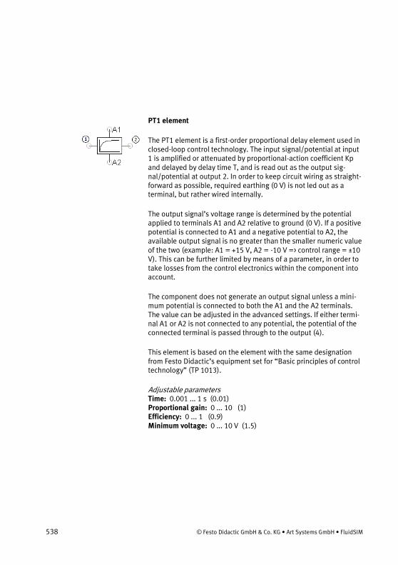
538 © Festo Didactic GmbH & Co. KG • Art Systems GmbH • FluidSIM
PT1 element
The PT1 element is a first-order proportional delay element used in closed-loop control technology. The input signal/potential at input 1 is amplified or attenuated by proportional-action coefficient Kp and delayed by delay time T, and is read out as the output sig-nal/potential at output 2. In order to keep circuit wiring as straight-forward as possible, required earthing (0 V) is not led out as a terminal, but rather wired internally.
The output signal’s voltage range is determined by the potential applied to terminals A1 and A2 relative to ground (0 V). If a positive potential is connected to A1 and a negative potential to A2, the available output signal is no greater than the smaller numeric value of the two (example: A1 = +15 V, A2 = -10 V => control range = ±10 V). This can be further limited by means of a parameter, in order to take losses from the control electronics within the component into account.
The component does not generate an output signal unless a mini-mum potential is connected to both the A1 and the A2 terminals. The value can be adjusted in the advanced settings. If either termi-nal A1 or A2 is not connected to any potential, the potential of the connected terminal is passed through to the output (4).
This element is based on the element with the same designation from Festo Didactic’s equipment set for “Basic principles of control technology” (TP 1013).
Adjustable parameters Time: 0.001 ... 1 s (0.01) Proportional gain: 0 ... 10 (1) Efficiency: 0 ... 1 (0.9) Minimum voltage: 0 ... 10 V (1.5)

© Festo Didactic GmbH & Co. KG • Art Systems GmbH • FluidSIM 539
PT2 element
The PT2 element is a second-order proportional delay element used in closed-loop control technology. The input signal/potential at input 1 is amplified or attenuated by proportional-action coefficient Kp and delayed by delay times T1 and T2, and is read out as the output signal/potential at output 2. In order to keep circuit wiring as straightforward as possible, required earthing (0 V) is not led out as a terminal, but rather wired internally.
The output signal’s voltage range is determined by the potential applied to terminals A1 and A2 relative to ground (0 V). If a positive potential is connected to A1 and a negative potential to A2, the available output signal is no greater than the smaller numeric value of the two (example: A1 = +15 V, A2 = -10 V => control range = ±10 V). This can be further limited by means of a parameter, in order to take losses from the control electronics within the component into account.
The component does not generate an output signal unless a mini-mum potential is connected to both the A1 and the A2 terminals. The value can be adjusted in the advanced settings. If either termi-nal A1 or A2 is not connected to any potential, the potential of the connected terminal is passed through to the output (4).
This element is based on the element with the same designation from Festo Didactic’s equipment set for “Basic principles of control technology” (TP 1013).
Adjustable parameters Time constant: 0.001 ... 1 s (0.01) Proportional gain: 0 ... 10 (1) Damping: 1e-5 ... 1000 s (1) Efficiency: 0 ... 1 (0.9) Minimum voltage: 0 ... 10 V (1.5)

540 © Festo Didactic GmbH & Co. KG • Art Systems GmbH • FluidSIM
Differential amplifier
The differential amplifier is a closed-loop control technology com-ponent. An output signal/potential is generated at output 3, which corresponds to the difference between the two input sig-nals/potentials at inputs 1 (w) and 2 (x). In the field of closed-loop control technology, the differential amplifier is used to determine deviation. In order to keep circuit wiring as straightforward as possible, required earthing (0 V) is not led out as a terminal, but rather wired internally.
The output signal’s voltage range is determined by the potential applied to terminals A1 and A2 relative to ground (0 V). If a positive potential is connected to A1 and a negative potential to A2, the available output signal is no greater than the smaller numeric value of the two (example: A1 = +15 V, A2 = -10 V => control range = ±10 V). This can be further limited by means of a parameter, in order to take losses from the control electronics within the component into account.
The component does not generate an output signal unless a mini-mum potential is connected to both the A1 and the A2 terminals. The value can be adjusted in the advanced settings. If either termi-nal A1 or A2 is not connected to any potential, the potential of the connected terminal is passed through to the output (4).
This element is based on the element with the same designation from Festo Didactic’s equipment set for “Basic principles of control technology” (TP 1013).
Adjustable parameters Efficiency: 0 ... 1 (0.9) Minimum voltage: 0 ... 10 V (1.5)
Limiter
The limiter is a closed-loop control technology component. Within a defined voltage range, the input signal/potential at input 1 is

© Festo Didactic GmbH & Co. KG • Art Systems GmbH • FluidSIM 541
replicated to another defined voltage range of the output sig-nal/potential. In order to keep circuit wiring as straightforward as possible, required earthing (0 V) is not led out as a terminal, but rather wired internally.
The voltage range of the input and output signals is specified after selecting the Operating mode option. The output signal is addition-ally limited by the potentials applied to terminals A1 and A2 relative to ground (0 V). If a positive potential is connected to A1 and a negative potential to A2, the available output signal is no greater than the smaller numeric value of the two (example: A1 = +15 V, A2 = -10 V => control range = ±10 V). This can be further limited by means of a parameter, in order to take losses from the control electronics within the component into account.
The component does not generate an output signal unless a mini-mum potential is connected to both the A1 and the A2 terminals. The value can be adjusted in the advanced settings. If either termi-nal A1 or A2 is not connected to any potential, the potential of the connected terminal is passed through to the output (4).
This element is based on the element with the same designation from Festo Didactic’s equipment set for “Basic principles of control technology” (TP 1013).
Adjustable parameters Operating mode: In [-10 V..10 V] –> Out [0 V..10 V], In [-10 V..10 V] –> Out [-10 V..10 V],Enter manually (In [-10 V..10 V] –> Out [0 V..10 V]) Efficiency: 0 ... 1 (0.9) Min. Voltage (in): -400 ... 400 V (-10) Max. Voltage (in): -400 ... 400 V (10) Min. Voltage (out): -400 ... 400 V (-10) Max. Voltage (out): -400 ... 400 V (10) Minimum voltage: 0 ... 10 V (1.5)

542 © Festo Didactic GmbH & Co. KG • Art Systems GmbH • FluidSIM
21.5.8 Controller (block diagram)
Summator
The summator element is a closed-loop control technology compo-nent. An output signal/potential is generated at output 4, which corresponds to the sum of the three input signals/potentials at inputs 1 through 3. In order to keep circuit wiring as straightfor-ward as possible, required earthing (0 V) and supply voltage are not led out as a terminals, but rather wired internally.
Adjustable parameters y offset: -5 ... 5 V (0)
D element
The D element is a transfer element used in closed-loop control technology with a derivative response characteristic. The output signal/potential at output 2 depends on the rate of change of the input signal/potential at input 1. The D element is modelled as an actual D element in this case, also known as a derivative-action element, with first-order time delay, because an ideal D element is technically infeasible. Derivative-action coefficient Kd and delay time T can be adjusted. In order to keep circuit wiring as straight-forward as possible, required earthing (0 V) and supply voltage are not led out as a terminals, but rather wired internally.
Adjustable parameters Derivation gain: 1 ... 1000 ms (2) Time constant (PT1): 0.01 ... 100 ms (0.8)

© Festo Didactic GmbH & Co. KG • Art Systems GmbH • FluidSIM 543
P element
The P element is a transfer element used in closed-loop control technology with a proportional response characteristic. The input signal/potential at input 1 is amplified by adjustable proportional-action coefficient Kp and read out as an output signal/potential at output 2. In the event of a proportional-action coefficient of less than 1, we no longer speak of amplification, but rather of attenua-tion. In order to keep circuit wiring as straightforward as possible, required earthing (0 V) and supply voltage are not led out as a terminals, but rather wired internally.
Adjustable parameters Proportional gain: 0 ... 1000 (1)
Hysteresis element
The hysteresis element acts as a two-step action controller with symmetrical hysteresis. If the input signal/potential at input 1 is increased to above the selected hysteresis value, output 2 auf is switched to +15 V. If the input signal/potential then drops to below the hysteresis value with a preceding minus sign, the output is switched to -15 V. In order to keep circuit wiring as straightforward as possible, required earthing (0 V) and supply voltage are not led out as a terminals, but rather wired internally.
Adjustable parameters Hysteresis: 0 ... 10 V (0) Minimum output voltage: -400 ... 400 V (-1) Maximum output voltage: -400 ... 400 V (1)
I element
The I element is a transfer element used in closed-loop control technology with an integral response characteristic. The input

544 © Festo Didactic GmbH & Co. KG • Art Systems GmbH • FluidSIM
signal/potential at input 1 is summed up over time and results in the output signal/potential at output 2. The speed at which the input signal is integrated can be adjusted with the integral-action coefficient. In order to keep circuit wiring as straightforward as possible, required earthing (0 V) and supply voltage are not led out as a terminals, but rather wired internally.
Adjustable parameters Integral gain: 1 ... 1000 1/s (100)
PT1 element
The PT1 element is a first-order proportional delay element used in closed-loop control technology. The input signal/potential at input 1 is amplified or attenuated by proportional-action coefficient Kp and delayed by delay time T, and is read out as the output sig-nal/potential at output 2. In order to keep circuit wiring as straight-forward as possible, required earthing (0 V) and supply voltage are not led out as a terminals, but rather wired internally.
Adjustable parameters Time: 0.001 ... 1 s (0.01) Proportional gain: 0 ... 10 (1)
PT2 element
The PT2 element is a second-order proportional delay element used in closed-loop control technology. The input signal/potential at input 1 is amplified or attenuated by proportional-action coefficient Kp and delayed by delay times T1 and T2, and is read out as the output signal/potential at output 2. In order to keep circuit wiring as straightforward as possible, required earthing (0 V) and supply voltage are not led out as a terminals, but rather wired internally.
Adjustable parameters Time constant: 1e-5 ... 1 s (0.01) Proportional gain: 0 ... 10 (1)

© Festo Didactic GmbH & Co. KG • Art Systems GmbH • FluidSIM 545
Damping: 1e-5 ... 1000 s (1)
Differential amplifier
The differential amplifier is a closed-loop control technology com-ponent. An output signal/potential is generated at output 3, which corresponds to the difference between the two input sig-nals/potentials at inputs 1 (w) and 2 (x). In the field of closed-loop control technology, the differential amplifier is used to determine deviation. In order to keep circuit wiring as straightforward as possible, required earthing (0 V) and supply voltage are not led out as a terminals, but rather wired internally.
Limiter
The limiter is a closed-loop control technology component. Within a defined voltage range, the input signal/potential at input 1 is replicated to another defined voltage range of the output sig-nal/potential. In order to keep circuit wiring as straightforward as possible, required earthing (0 V) and supply voltage are not led out as a terminals, but rather wired internally.
The voltage range of the input and output signals is specified after selecting the Operating mode option.
Adjustable parameters Operating mode: In [-10 V..10 V] –> Out [0 V..10 V], In [-10 V..10 V] –> Out [-10 V..10 V],Enter manually (In [-10 V..10 V] –> Out [0 V..10 V]) Min. Voltage (in): -400 ... 400 V (-10) Max. Voltage (in): -400 ... 400 V (10) Min. Voltage (out): -400 ... 400 V (-10) Max. Voltage (out): -400 ... 400 V (10)

546 © Festo Didactic GmbH & Co. KG • Art Systems GmbH • FluidSIM
21.6 Digital Components
21.6.1 Constants and Terminals
Digital input
Digital inputs are designated with an “I”. In FluidSIM digital com-ponents can be used inside and outside a digital module. If a digital input is used inside a digital module, you can determine the input connector of the digital module in question with which the digital input shall be linked by allocating a number “I1” to “I16”. If there is an analog signal of more than 10V at the chosen input of the digital module, the digital input is set to “Hi”. If a digital input is used outside a digital module, there is an additional analog electri-cal connection at the digital input. If there is an analog signal of more than 10V at this connection, the digital input is set to “Hi”. As an alternative you can click on the digital input with the left mouse button in order to set it to “Hi”. Another click resets the value to “Lo”.
Digital output
Digital outputs are designated with an “Q”. The output connects a digital signal through from its input to its output. In FluidSIM digital components can be used inside and outside a digital module. If a digital output is used inside a digital module, you can determine the output connector of the digital module in question with which the digital output shall be linked by allocating a number “Q1” to “Q16”. If the status of the digital output is “Hi”, a potential of 24V is set at the corresponding output connector of the digital module. If a digital output is used outside a digital module, there is an additional analog electrical connection at the digital output. If the status of the digital output is “Hi”, a potential of 24 V is set at this connection.

© Festo Didactic GmbH & Co. KG • Art Systems GmbH • FluidSIM 547
Memory bits
Memory bits are designated with a “M”. Memory bits are virtual outputs, with a value at their output analog to that at their input. When the simulation start is activated, you can define by using the property dialog box if the output Q shall be set to “Lo” or to “Hi”, independent on the input value. After the simulation start the value at the output is set to the value of the input.
Adjustable parameters Initial state = Hi: ... (false)
Logic level HI
At the output Q you have the logic level “Hi”.
Logic level LO
At the output Q you have the logic level “Lo”.
Connection (digital)
An digital connection is a place where a digital line can be attached to. To simplify the line drawing process, a connection appears as a small circle in Edit Mode. Note that at each digital connection its level “Lo” / “Hi” can be displayed.
Line (digital)
A digital line links two digital connections. Note that a digital con-nection may be a simple digital connection or a T-junction.

548 © Festo Didactic GmbH & Co. KG • Art Systems GmbH • FluidSIM
T-junction (digital)
A T-junction joins up to four digital lines, thus having a single digital level. Note that T-junctions are introduced automatically by FluidSIM when dropping the line drawing cursor onto another line in Edit Mode.
21.6.2 Basic Functions
AND
The output Q of the AND is only “Hi” when all inputs are “Hi”, that is, if they are closed. If an input pin of this module is not connected, its status is automatically “Hi”.
Edge-triggered AND
The output Q of the edge-triggered AND is only “Hi” when all inputs are “Hi” and if at least one input was “Lo” in the previous cycle. If an input pin of this block is not connected, its status is automatical-ly “Hi”.
NAND (AND not)
The output Q of the NAND is only “Lo”, when all inputs are “Hi”, that is, if they are closed. If an input pin of this block is not con-nected, its status is automatically “Hi”.

© Festo Didactic GmbH & Co. KG • Art Systems GmbH • FluidSIM 549
NAND With Edge Evaluation
The output Q of the NAND with edge evaluation is only “Hi”, if at least one input is “Lo” and if all inputs were “Hi” in the previous cycle. If an input pin of this block is not connected, its status is automatically “Hi”.
OR
The output Q of the OR is only “Hi”, if at least one input is “Hi”, that is, if it is closed. If an input pin of this block is not connected, its status is automatically “Lo”.
NOR (OR not)
The output Q of the NOR is only “Hi” when all inputs are “Lo”, that is, if they are switched off. As soon as any input is switched on (status “Hi”), the output of the NOR is set to “Lo”. If an input pin of this block is not connected, its status is automatically “Lo”.
XOR (exclusive OR)
The output Q of the XOR is “Hi”, if the inputs are nonequivalent. If an input pin of this block is not connected, its status is automatical-ly “Lo”.
NOT (Negation, Inverter)
The output Q is “Hi” if the input is “Lo”. The NOT block is an input status inverter.

550 © Festo Didactic GmbH & Co. KG • Art Systems GmbH • FluidSIM
21.6.3 Special Functions
Digital module
The digital module is used for a compact embedding of a digital switching circuit into a electropneumatic or electrohydraulic circuit. The digital module offers 8 (16) electrical inputs and outputs, which transfer their states to its digital switching circuit in the inner part. Therefore the digital switching circuit does not need much space in the electropneumatic or electrohydraulic circuit for the display of the digital module as a rectangle with a total number of 18 (34) connections. By making a double-click with the left mouse button on the digital module you come to the digital circuit in the inner part of the module. A new window opens. It shows the digital circuit and can be handled in the usual way. The standard configuration in the inner part of a new inserted digital module is a row with 8 (16) inputs and 8 (16) outputs each. They correspond to the inputs and outputs of the module in the electropneumatic or electrohydraulic circuit. In order to be able to test the digital circuit during the setup, it can be simulated separated from the electropneumatic or elec-trohydraulic circuit. As soon as the processing window of the digital module is closed or the original circuit window is put into the fore-ground, the previously effected changes in the digital circuit are automatically adopted into the digital module of the electropneumatic or electrohydraulic circuit. Inside the digital module only digital components can be inserted. Furthermore, an encapsulating of additional digital modules inside a module is not possible. However, you can use several digital modules in one electropneumatic or electrohydraulic circuit. Please note that the digital circuit inside a digital module only works correctly if corre-sponding potentials are set at the electrical power supply units of the module (+24 V) and (0 V).
On delay
An output with on delay is not switched on until a specified time has expired. When the status of input Trg changes from “Lo” to

© Festo Didactic GmbH & Co. KG • Art Systems GmbH • FluidSIM 551
“Hi”, the on delay time starts. If the status of input Trg is “Hi” at least for the duration of the configured time, the output Q is set to “Hi” on expiration of this time. The output follows the input with on delay. The time is reset, when the status of the input changes again to “Lo” before the time has expired. The output is reset to “Lo”, when the status at the input is “Lo”.
Adjustable parameters Delay time: 0 ... 100 s (3)
Off delay
The output is not reset until a configured time has expired. When the input status turns to “Hi”, the output Q is switched instantane-ously to “Hi”. If the status at input Trg changes from “Hi” to “Lo”, the off delay starts. After expiration of the configured time, the output is reset to “Lo” (off delay). When the input Trg is switched on and off again, the off delay restarts. The input R (Reset) is used to reset the delay time and the output before the configured time has expired.
Adjustable parameters Delay time: 0 ... 100 s (3)
On/Off delay
An output with on/off delay is switched on after a specified time and is reset on expiration of a second specified time. As soon as the status at input Trg changes from “Lo” to “Hi”, the configured on delay time starts. If the status at input Trg remains “Hi” at least for the duration of the configured time, the output Q is set to “Hi” on expiration of the on delay time (the output follows the input on delayed). If the status at input Trg changes again to “Lo”, before the configured on delay time has expired, the time is reset. When the status at input returns to “Lo”, the configured off delay time starts. If the status at the input remains “Lo” at least for the dura-tion of the configured off delay time, the output is set to “Lo” on

552 © Festo Didactic GmbH & Co. KG • Art Systems GmbH • FluidSIM
expiration of that time (the output follows the input off delayed). If the status at the input returns to “Hi” before this time has expired, the time is reset.
Adjustable parameters On delay time: 0 ... 100 s (3) Off delay time: 0 ... 100 s (6)
Retentive On delay
A specified time starts after an input pulse. The output is set on expiration of this time. As soon as the status at the input Trg changes from “Lo” to “Hi”, the specified time starts. After expira-tion on the configured time, the output Q is set to “Hi”. Further switching actions at input Trg have no influence on the running time. The output and the time are only reset to “Lo” when the status at input R is “Hi”.
Adjustable parameters Delay time: 0 ... 100 s (3)
Latching Relay
Input S sets output Q. Another input R resets the output Q. A latch-ing relay is a simple logic memory. The output value depends on the input states and on the previous output status.
Pulse Relay
A short oneshot at the input is used to set and reset the output. Output Q status is toggled at every “Lo” to “Hi” transition of the status at input Trg, that is, the output is switched on or off. Use input R to reset the pulse relay to initial state, that is, the output is set to “Lo”.

© Festo Didactic GmbH & Co. KG • Art Systems GmbH • FluidSIM 553
Wiping Relay - Pulse Output
An input signal generates a signal of specified length at the output. The output status is switched to “Hi” after the input Trg is set to “Hi”. The configured time is started at the same time and the out-put remains set. After expiration of the configured time, the output is reset to the status “Lo” (pulse output). If the input status chang-es from “Hi” to “Lo” before the specified time has expired, also the output follows immediately with a with a “Hi” to “Lo” transition.
Adjustable parameters Delay time: 0 ... 100 s (3)
Edgetriggered Wiping Relay
An input signal generates a signal of specified length at the output (retriggering). The output status is switched to “Hi” after the input Trg is set to “Hi”. The configured time is started at the same time. After expiration of the configured time, the output Q status is reset to “Lo” (pulse output). If the input status changes again from “Lo” to “Hi” (retriggering), before the specified time has expired, the time is reset and the output remains switched on.
Adjustable parameters Delay time: 0 ... 100 s (3)
Timer Switch
With the timer switch you can create timer switches referring to days, weeks and years. Upon reach of the specified on-transition time, the output Q of the timer switch is set to “Hi” and upon reach of the specified off-transition time to “Lo”. If you have chosen the option “Repeat every”, the on and off transition is repeated each time according to the specified repetition time.

554 © Festo Didactic GmbH & Co. KG • Art Systems GmbH • FluidSIM
Adjustable parameters On time: 0 ... 1000 s (10) Off time: 0.1 ... 1000 s (30) Repeat every: 0.1 ... 1000 s (60)
Up/Down Counter
Depending on the configuration of the input Dir, an internal value is counted up or down through an input pulse. The output is set when the configured count value is reached. With every status change at the input Cnt from “Lo” to “Hi”, the internal counter is increased (Dir = “Lo”) or decreased (Dir = “Hi”) by one unit. If the internal counter is equal or larger compared to the specified value, the output Q is set to “Hi”. You can use the reset input R to reset the internal count value and the output to “Lo”. As long as R=“Hi”, also the output is “Lo” and the pulses at input Cnt are not counted.
Adjustable parameters Counter: 0 ... 9999 (5)
Symmetric Clock Generator
A timing signal with a configurable period is given at the output. Via the duration of the pulses you can determine the length of the on and off times. Via the input En (for Enable) you can switch on the clock generator, that is, the clock generator sets the output to “Hi” for the duration of the pulse, subsequent the output to “Lo” for the duration of the pulse and so on, until the input status is “Lo” again.
Adjustable parameters Impulse time: 0.0005 ... 100 s (0.5)

© Festo Didactic GmbH & Co. KG • Art Systems GmbH • FluidSIM 555
Asynchronous Pulse Generator
The pulse profile of the output can be changed via the configurable pulse duration and pulse pause duration. It is possible to invert the output with input INV. The input INV only negates the output, if the block is enabled via EN.
Adjustable parameters Impulse time: 0.01 ... 100 s (3) Impulse pause time: 0.01 ... 100 s (1)
Frequency Threshold Trigger
The output is switched on and off depending on two frequencies which can be specified. The threshold trigger measures the signals at input Fre. The pulses are captured across a measuring interval which can be specified. If the frequency measured within the meas-uring interval higher than the input frequency, the output Q is switched to “Hi”. Q is switched again to “Lo” when the measured frequency has reached the value of the output frequency or if it is lower.
Adjustable parameters On frequency: 0.01 ... 9999 Hz (6) Off frequency: 0.01 ... 9999 Hz (2) Time interval: 0.001 ... 100 s (5)

556 © Festo Didactic GmbH & Co. KG • Art Systems GmbH • FluidSIM
21.7 GRAFCET Elements
21.7.1 GRAFCET
Step
The name of a step may contain the following characters: “0-9”, “a-z”, “A-Z” and the underscore “_”. You can select from the following seven different step types: simple step, initial step, macro-step, macro input, macro output, enclosing step and initial enclosing step. Furthermore, you can give the step an activation link.
Transition
You can give a transition a name, which is shown to the left of the transition in brackets. Entering a transition condition is supported by buttons for special symbols (AND, OR, NOT, falling edge, rising
edge, delay). Via Variable you can select an existing GRAFCET
variable from a list. Alternatively to the formula, you can show a descriptive text. To do this, you have to select the option “Display description instead of formula”. In the “Connection ID/target in-formation” field, you can enter a step that links to the transition’s output without having to draw a connecting line. You can select an existing step from a list.
Action
There are three types of action: assignations, allocations and compulsory commands. For assignations and allocations, you can enter a variable or an output, whose value is changed by the action. The name of a variable may contain the following characters: “0-9”, “a-z”, “A-Z” and the underscore “_”. For a “conditional action” or

© Festo Didactic GmbH & Co. KG • Art Systems GmbH • FluidSIM 557
an “Action on event”, you can enter a condition that has to be fulfilled before the action is executed. Entering a condition is sup-ported by buttons for special symbols (AND, OR, NOT, falling edge,
rising edge, delay). Via Variable you can select an existing
GRAFCET variable from a list. Alternatively to the formula, you can show a descriptive text. To do this, you have to select the option “Display description instead of formula”. For an allocation (“action on activation”, “action on deactivation” and “action on event”), you can enter any term whose value is to be allocated to the action variable. Entering a term is supported by buttons for special sym-
bols (AND, OR, NOT, falling edge, rising edge). Via Variable you
can select an existing GRAFCET variable from a list. Alternatively to the formula, you can show a descriptive text. To do this, you have to select the option “Display description instead of formula”. For a “compulsory command”, you can enter the name of the partial GRAFCET directly or select an existing partial GRAFCET from a list. You can also enter the relevant steps directly or select them from a list of existing steps. You have to separate the step names with commas. You can select the special commands “*” and “INIT” using the relevant buttons.
Synchronization
You can connect synchronizations like other FluidSIM components. However, they do not initially have any connections. You always have to draw connecting lines to a synchronization. The corre-sponding connections are then generated automatically.
Partial GRAFCET
If you want to allocate GRAFCET elements to a specific partial GRAFCET, place the partial GRAFCET frame over the relevant GRAFCET part and give it a name. The preceding “G” is not part of the name that you have to enter; it is added automatically by FluidSIM and shown at the bottom left of the partial GRAFCET frame. You can alter the size of the partial GRAFCET frame by drag-ging its edges with the mouse. For the partial GRAFCET to function correctly, it is important that all its elements are completely within

558 © Festo Didactic GmbH & Co. KG • Art Systems GmbH • FluidSIM
the frame and that the frame does not overlap with any foreign elements or other frames.
GRAFCET-PLC-Component
The GRAFCET-PLC component is similar to a SPS controller, whose behavior is described by a GRAFCET. For more information, please read the section GRAFCET-PLC-Component.
GRAFCET-PLC-Component
The GRAFCET-PLC component is similar to a SPS controller, whose behavior is described by a GRAFCET. For more information, please read the section GRAFCET-PLC-Component.
GRAFCET-PLC-Component
The GRAFCET-PLC component is similar to a SPS controller, whose behavior is described by a GRAFCET. For more information, please read the section GRAFCET-PLC-Component.
GRAFCET-I/O
The GRAFCET I/O component is used to link the GRAFCET variables with the electrical part of a circuit. You can enter eight GRAFCET input variables and eight GRAFCET output variables into the GRAFCET I/O component. The actions' variables serve as outputs. The inputs can be the allocations and conditions of actions and transitions. If a potential is created as the input of the GRAFCET I/O component, the corresponding variable is set to “1”. If an output variable has a value other than “0”, a potential of 24V is created at the corresponding output of the GRAFCET I/O component.

© Festo Didactic GmbH & Co. KG • Art Systems GmbH • FluidSIM 559
21.8 Miscellaneous
21.8.1 Miscellaneous
Connection (mechanical)
A mechanical connection constitutes a place holder for the label of a valve solenoid. To simplify clicking, a mechanical connection appears as a small circle in Edit Mode.
Valve solenoid
The valve solenoid switches the valve. By means of a label the valve solenoid can be linked to a valve that is solenoid operated.
Adjustable parameters Resistance: 1 ... 10000 Ohm (90) Minimum voltage: 0.1 ... 300 V (20)
Proportional valve solenoid, position controlled
In FluidSIM the proportional valve solenoid is coupled to the re-spective continuous directional valve with the help of a label. The required slide position is predetermined via a voltage signal. The valve slide distance is position controlled. The control and amplifier component is integrated in the valve.
Adjustable parameters Current (max): 0.01 ... 10 A (0.1) Resistance: 1 ... 10000 Ohm (128)

560 © Festo Didactic GmbH & Co. KG • Art Systems GmbH • FluidSIM
Minimum voltage: 0.1 ... 300 V (20)
Proportional amplifier, 1-channel
The amplifier is used to control proportional valves. For this pur-pose, nominal values (voltage signals) from 0 V to +10 V are trans-formed into the necessary magnetic current for the proportional valves. In FluidSIM the amplifier is coupled to the respective valve with the help of a label. The maximum current at the amplifier output is hereby automatically adjusted in relation to the coupled valve. A step current relative to the maximum current can be speci-fied, in order to compensate the positive overlap of proportional valves. The amplifier requires a power supply of 24 V.
Adjustable parameters Current (max): 0.01 ... 30 A (0.1) Jump current: 0 ... 25 % (0) Resistance: 1 ... 10000 Ohm (100) Minimum voltage: 0.1 ... 300 V (20)
Proportional amplifier, 2-channel
The amplifier is used to control proportional valves with two mag-nets. For this purpose, nominal values (voltage signals) from -10 V to +10 V are transformed into the necessary magnetic current for the proportional valves. Output A is gated at a nominal value be-tween 0 V and -10 V, output B between 0 V and -10 V. In FluidSIM the amplifier is coupled to the respective valve with the help of two labels. The maximum currents at the amplifier outputs are hereby automatically adjusted in relation to the coupled valves. A step current relative to the maximum current can be specified, in order to compensate the positive overlap of proportional valves. The amplifier requires a power supply of 24 V.
Adjustable parameters Current (max): 0.01 ... 30 A (0.1) Jump current: 0 ... 25 % (0)

© Festo Didactic GmbH & Co. KG • Art Systems GmbH • FluidSIM 561
Resistance: 1 ... 10000 Ohm (100) Minimum voltage: 0.1 ... 300 V (20)
Valve solenoid (ladder)
The valve solenoid switches the valve. By means of a label the valve solenoid can be linked to a valve that is solenoid operated.
Adjustable parameters Resistance: 1 ... 10000 Ohm (90) Minimum voltage: 0.1 ... 300 V (20)
Distance rule
The distance rule is a device for attaching switches at the cylinder. The labels at the distance rule define links to the actual proximity switches or limit switches in the electrical circuit.
Status indicator
In Edit Mode, the status indicator is automatically displayed at those components that are actuated in the circuit’s initial position.
Cam switch
In Edit Mode, the cam switch is automatically displayed at those mechanically operated way valves that are actuated in the circuit’s initial position.
Text

562 © Festo Didactic GmbH & Co. KG • Art Systems GmbH • FluidSIM
The concept of text components in FluidSIM gives the user a way in which to describe components in diagrams, assign identification texts, or to provide commentary on the diagram. The text and the appearance of text components can be customized to the user’s liking.
State diagram
The state diagram records the state quantities of important compo-nents and depicts them graphically.
Terminal assignment diagram
The terminal assignment diagram list automatically creates termi-nals in the electrical circuit and displays the allocation in a table.
Functional diagram
With the functional diagram editor, functional diagrams e.g. dis-placement-step diagrams can be created.
Parts list
The parts list component creates from the components of a circuit diagram a table, which contains for each component its designation and its description.
Rectangle
Rectangles are graphic primitives, which can also be used within circuit diagrams.

© Festo Didactic GmbH & Co. KG • Art Systems GmbH • FluidSIM 563
Ellipse
Ellipses are graphic primitives, which can also be used within circuit diagrams.
Bitmap
In FluidSIM images, as with all other components and objects, can be inserted, positioned, moved, rotated and mirrored. In addition, images such as rectangles and ellipses are freely scalable.

Learning, Teaching, and Visualizing Technologies
564 © Festo Didactic GmbH & Co. KG • Art Systems GmbH • FluidSIM
Chapter 2222. Learning, T eachi ng, a nd Visual izi ng Technol ogies
Beside the creation and simulation of electro-fluidic circuit dia-grams, FluidSIM also supports teaching basic knowledge. This knowledge is presented in the form of texts, overview pictures, sectional views, exercises, and educational films. Functions that realize the selection of this instruction material are found under the
Didactics menu.
One group of these functions refers to information about single, selected components. Another group of functions refers to ordered overviews of the didactics material, allowing the selection of an interesting topic. Finally, it is also possible to select and link to-
gether arbitrary topics into so-called Presentation... .
Appendix Component Library and Didactics Material offer a
complete and concise summary of the instructional material in FluidSIM.
The following sections contain a description of the functions found
under the Didactics menu.
22.1 Information about Single Components
The first three entries under the Didactics menu refer to selected
components and are context sensitive. More precisely:
When a component in the current circuit diagram window is select-ed, or all selected components are of the same type, the menu
entry Component description will be enabled.

© Festo Didactic GmbH & Co. KG • Art Systems GmbH • FluidSIM 565
22.1.1 Component Descriptions
All components possess a page with a technical description. This page contains the diagram symbol for the component according to the DIN standard (“Deutsche Industrienorm”), a textual description of the component’s function, the designations of the connections, and a listing of the adjustable parameters along with their value ranges.
You will find a photograph of the real-life part provided for most components. In the case that a component cannot exist singularly in a real system, FluidSIM displays a photo of the assembly group that this component belongs to. Examples for such components include the indicator light, relays, switches, and the electrical power supply. Components, that do not exist in reality, simply have no photo. Examples include the text component and the distance rule.
→ Select the one-way flow control valve and click on the menu
item Component description under the Didactics menu.
The following page opens:
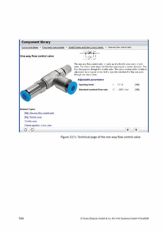
566 © Festo Didactic GmbH & Co. KG • Art Systems GmbH • FluidSIM
Figure 22/1: Technical page of the one-way flow control valve
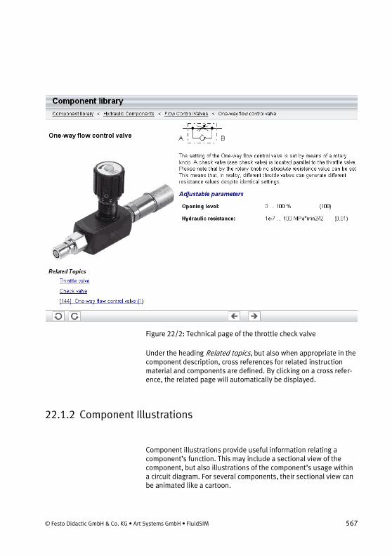
© Festo Didactic GmbH & Co. KG • Art Systems GmbH • FluidSIM 567
Figure 22/2: Technical page of the throttle check valve
Under the heading Related topics, but also when appropriate in the component description, cross references for related instruction material and components are defined. By clicking on a cross refer-ence, the related page will automatically be displayed.
22.1.2 Component Illustrations
Component illustrations provide useful information relating a component’s function. This may include a sectional view of the component, but also illustrations of the component’s usage within a circuit diagram. For several components, their sectional view can be animated like a cartoon.

568 © Festo Didactic GmbH & Co. KG • Art Systems GmbH • FluidSIM
→ Select an air motor (4/2-way hand-lever valve in case of hy-
draulic version) and click on Component description under
the Didactics menu.
The following dialog box appears:

© Festo Didactic GmbH & Co. KG • Art Systems GmbH • FluidSIM 569
Figure 22/3: Page component-specific topics

570 © Festo Didactic GmbH & Co. KG • Art Systems GmbH • FluidSIM
Figure 22/4: Dialog box with component-specific topics
→ Please click the line with the relevant topic [35] Air motor (hydraulics: [104] 4/2-way valve, two pistons (1) ).
The following picture appears:

© Festo Didactic GmbH & Co. KG • Art Systems GmbH • FluidSIM 571
Figure 22/5: Function illustration of a air motor

572 © Festo Didactic GmbH & Co. KG • Art Systems GmbH • FluidSIM
Figure 22/6: Function illustration of a 4/2-way valve
Often it is easier to understand the functional nature of a compo-nent, when its behavior is visualized through the use of animation. For this reason, several components possess different sectional views showing the component at different states. These sectional views can be animated in much the same way as a flip book.
→ Please mark a quick-exhaust valve(hydraulics: 3-way pressure
reducing valve)and click the menu option Didactics Compo-
nent description to open the window with the component de-
scription. Now click the link with the function illustration [87] quick exhaust valve (hydraulics: [84] 3-way pressure reducing valve)
This function illustration can be animated.
→ Click on or Execute Start to start the animation.

© Festo Didactic GmbH & Co. KG • Art Systems GmbH • FluidSIM 573
An animation can be “frozen” with or by clicking on Pause in
the Execute menu. or Execute Stop stops an animation,
whereas or Execute Reset restarts an animation.
22.2 Selecting Didactics Material from a List
The entries Tutorial ’Simulating with FluidSIM' , Component
Library and Didactics Material under the Didactics menu
present the didactics material of FluidSIM organized in the form of overview pages. From these pages topics can be chosen and viewed independently of the current window and possibly selected components.
22.2.1 Tutorial
Below this menu option you can launch the tutorial “Simulating with FluidSIM”, which contains a variety of interesting experiments and an excursus. By means of these useful examples you will get to know the possibilities of simulating with FluidSIM. Furthermore, for the most important components the mathematic models used in FluidSIM are also described.
→ Please click the menu option Didactics Tutorial ’Simulating
with FluidSIM' to open the tutorial.

574 © Festo Didactic GmbH & Co. KG • Art Systems GmbH • FluidSIM
Figure 22/7: Tutorial (Pneumatics)

© Festo Didactic GmbH & Co. KG • Art Systems GmbH • FluidSIM 575
Figure 22/8: Tutorial (Hydraulics)
On the right-hand side the hierarchical directory is displayed. By double-clicking the directory symbols you may list off or close the applicable subsections. Clicking a page symbol will display the contents of the page in the open window.
22.2.2 Component Library
Below the menu option Component Library you will find descrip-
tions and photos of all FluidSIM -components.
→ Click a menu option Didactics Component Library to open
the help pages of the component library.

576 © Festo Didactic GmbH & Co. KG • Art Systems GmbH • FluidSIM
Figure 22/9: Component Library (Pneumatics)

© Festo Didactic GmbH & Co. KG • Art Systems GmbH • FluidSIM 577
Figure 22/10: Component Library (Hydraulics)
22.2.3 Didactics Material
FluidSIM, alongside the tutorial and the component reference, contains further didactics material particularly useful for group work. Moreover, here you will find educational films, provided you have copied them onto the hard disk during the installation. If you haven’t installed the film files, you may choose a chapter via the
menu option Didactics Educational Film... to view the applicable
film from the included video-CD.
→ Click the menu option Didactics Didactics Material to open
the overview of the didactics material.

578 © Festo Didactic GmbH & Co. KG • Art Systems GmbH • FluidSIM
Figure 22/11: Didactics Material (Pneumatics)

© Festo Didactic GmbH & Co. KG • Art Systems GmbH • FluidSIM 579
Figure 22/12: Didactics Material (Hydraulics)
22.3 Presentations: Combining Instructional Material
Sometimes you may want to examine a topic from different angles or combine individual topics into a lesson. For this purpose
FluidSIM offers the concept entitled Presentation... .
There are a number of already prepared presentations, which can be found on the FluidSIM installation disks. However, editing presentations or creating new presentations is also possible with
FluidSIM. All presentations can be found under Presentation... in
the Didactics menu.
→ Click on Didactics Presentation... .

580 © Festo Didactic GmbH & Co. KG • Art Systems GmbH • FluidSIM
The following dialog box appears:

© Festo Didactic GmbH & Co. KG • Art Systems GmbH • FluidSIM 581
Figure 22/13: Dialog box for selecting and editing presentations (Pneumatics)

582 © Festo Didactic GmbH & Co. KG • Art Systems GmbH • FluidSIM
Figure 22/14: Dialog box for selecting and editing presentations (Hydraulics)
This field contains a list of already created presentations.
Clicking on “ New presentation... ” opens a second dialog box for
the creation of a new presentation.
Clicking on “ Edit presentation... ” opens a second dialog box to
begin editing a presentation.
When the “Preview” setting is activated, the picture that pertains to the selected presentation appears underneath the topics list.
→ Click on “New Presentation” to open the following dialog box.
Presentations
New presentation...
Edit presentation...
Preview

© Festo Didactic GmbH & Co. KG • Art Systems GmbH • FluidSIM 583
Figure 22/15: Dialog box for editing presentations (Pneumatics)

584 © Festo Didactic GmbH & Co. KG • Art Systems GmbH • FluidSIM
Figure 22/16: Dialog box for editing presentations (Hydraulics)
In this text field a short description of the presentation can be entered. This text may consist of up to 128 characters and will appear with the other presentations, the next time the presentation dialog box is opened.
This field contains a list of all available topics dealing with “ Pneu-matics basics”, “Hydraulics basics”, “Working principle”, and “Exercise”. Moreover, there exist two pictures that can be used to announce a refreshment and a lunch break respectively. A double click on a line in the “Available Topics” list inserts this line in the “Selected topics” list above the highlighted bar. In this way a presentation can be created or altered. Moreover, a user can inte-grate his own circuit diagrams, DXF files, BMP- and WMF-picture files, or even multimedia files such as sounds or video clips. To do
Description
Available topics

© Festo Didactic GmbH & Co. KG • Art Systems GmbH • FluidSIM 585
so, click on “User file”: A dialog box opens that allows for the selection of the desired data source on the file system.
This field contains a list of topics chosen for the current presenta-tion.
Clicking on “ Add ” is the same as double clicking a line in the “
Available topics ” list: The selected line in “ Available topics ” will be inserted in the “ Selected topics ” list.
Clicking on “ Delete ” deletes the selected line of the “ Selected
topics ” list.
When the “ Preview ” setting is activated, the picture that pertains to the selected topic appears underneath the respective list.
Within both topics lists the highlighted bar can be moved using the arrow keys. Maybe it will be necessary to click and select the list you want to work with. After creating a new presentation and clos-
ing the dialog box by clicking on “ &OK ”, FluidSIM asks you to
name the presentation file. Presentation files have the extension .shw and are located in the subdirectory shw under the installa-
tion directory.
22.4 Extended Presentations in the Microsoft PowerPoint Format
The hydraulics version of FluidSIM contains an additional large set of presentations written in the Microsoft PowerPoint Format. To use these presentations, PowerPoint must not be installed on your PC since FluidSIM installs the necessary viewer at its installation time.
→ Click on Extended Presentation... to open the dialog box of a
presentation.
Selected topics
Add
Delete
Preview

586 © Festo Didactic GmbH & Co. KG • Art Systems GmbH • FluidSIM
Figure 22/17: Selection of an extended presentation
→ Select the item “Actuators” to open the related presentation in full screen mode.
Most of the topics form a picture sequence, which can be viewed in a single-step manner using the left mouse button or the spacebar.
→ Move two single steps forward in the current presentation.

© Festo Didactic GmbH & Co. KG • Art Systems GmbH • FluidSIM 587
Figure 22/18: Actuators
When clicking the right mouse button, a context menu is opened by which, among others, the presentation can be closed or particular pictures picked out. The files of the extended presentations are in the subdirectory ppx of the FluidSIM installation. You can add
new PowerPoint presentations on your own by copying the related files (format: “ppt” or “pps”) into the ppx -directory. Like the
other didactics material (illustrations of function, component pho-tos, circuit drawings, educational films, etc.), the PowerPoint presentations can linked and used within presentations (cf. Section Presentations: Combining Instructional Material).

Didactics Material Survey (Pneumatics)
588 © Festo Didactic GmbH & Co. KG • Art Systems GmbH • FluidSIM
Chapter 2323. Didactics Material Survey (Pne umatics)
This chapter provides a comprehensive listing of those parts of the didactics material in FluidSIM that are not covered by chapter The Component Library “The Component Library” . Basically, this mate-rial consists of the components' behavior illustrations, the anima-tions, the exercises, and the educational films, which all can be
activated under the Didactics menu. The subsequent sections
are arranged thematically. The icon indicates that an animation exists for the related topic. The last section gives an overview of the educational films.
23.1 Basics
[1] Pneumatic system structure and signal flow
A pneumatic system can be broken down into a number of levels representing the hardware and signal flow from the energy source to the actuating devices.
→ The topic highlights the relationship between signals, levels and elements in a pneumatic system.
[2] Circuit diagram and pneumatic elements
Circuit diagrams are drawn in such a way that signals, for instance energy or potential values, are oriented downwards. The number-ing of the components is derived from their respective function in the diagram.
→ The topic highlights the various levels in a circuit.

© Festo Didactic GmbH & Co. KG • Art Systems GmbH • FluidSIM 589
[3] Designating the elements, circuit diagram
This topic shows the relationship between levels in a circuit.
[4] Designating the elements, circuit diagram
The figures contrasts the position of a roller lever valve (initial position: actuated by the cylinder) in a circuit diagram and its physical setup in a plant.
[5] Designating the elements, circuit diagram
The figures contrasts the position of a roller lever valve (initial position: not actuated) in a circuit diagram and its physical setup in a plant.
[6] Designating the elements, circuit diagram
All elements should be shown in the circuit diagram in the initial position. If valves have been drawn with an actuated initial posi-tion, this fact is indicated for example by an arrow, or for a limit switch, by drawing the cam.
→ Explain the differences between the following terms: initial position and starting position.

590 © Festo Didactic GmbH & Co. KG • Art Systems GmbH • FluidSIM
23.2 Supply elements
[7] Symbols of energy and supply components, supply and ser-vice equipment
The Symbols are from the DIN ISO 1219 “Circuit symbols for fluidic power components and systems”. The symbols for the energy supply system can be represented as individual components or as combined elements.
→ Compare the symbols with the combined symbols (topic 8).
[8] Symbols of energy and supply components, combined sym-bols
In general where specific technical details are to be given, such as requirements for non-lubricated air or micro-filtering, the complete detailed symbol should be used. If a standard and common air supply is used for all components, the simplified symbols can be used.
→ Compare the symbols with the previous topic.
[9] Air service unit
The filter is normally combined with the pressure regulator and lubricator to form a compressed air service unit. The selection of the correct filter plays an important role in determining the quality and performance of the control system which is to be supplied with compressed air.
→ Refer to topic 10 for construction of the filter.

© Festo Didactic GmbH & Co. KG • Art Systems GmbH • FluidSIM 591
[10] Compressed air filter
The compressed air passes through a baffle plate in the filter bowl. The air is rotated, and the heavier dust particles and water droplets are spun by centrifugal force against the inner wall of the filter bowl and run down the wall of the housing. The air which has been precleaned then passes through the filter element.
→ The bowl must be emptied daily to prevent overflow.
[11] Air drying, low temperature
The lower the dew point the more the water will condense and reduce the amount entrapped in the air. Using refrigeration meth-ods, it is possible to achieve dew points of between 2°{C} and 5°{C}.
→ Compare with absorption and adsorption drying.
[12] Air drying, absorption
Absorption drying is a purely chemical process. The moisture in the compressed air forms a compound with the drying agent in the tank. This causes the drying agent to break down; it is then dis-charged as a fluid at the base of the tank. The drying agent must be replenished at a rate which is dependent on the compressed air temperature, water content and flow rate.
→ Compare with adsorption drying.

592 © Festo Didactic GmbH & Co. KG • Art Systems GmbH • FluidSIM
[13] Air drying, adsorption
The lowest equivalent dew points (down to -90°{C}) can be achieved by means of adsorption drying. In this process, the com-pressed air is passed through gel and the water is deposited on the surface, i.e. it is adsorbed.
→ Compare with absorption drying.
[14] Air lubricator
As a rule, the compressed air which is generated should be dry and free of oil. For some components, lubricated air is damaging, for others, it is undesirable, and for power components, it may in certain cases be necessary. Lubrication of the air should therefore be limited to the sections of the plant which require it.
→ Refer to picture of topic 9 for general arrangement.
[15] Air lubricator
Air passing through the lubricator causes a pressure drop between the oil reservoir and the upper part of the lubricator. This pressure difference forces the oil upwards through a tube and it then drips into a nozzle which can be seen through an inspection glass. The oil is atomized and carried along by the air stream.
→ It is necessary to carefully adjust the oil discharge rate.

© Festo Didactic GmbH & Co. KG • Art Systems GmbH • FluidSIM 593
[16] Pressure regulator with vent hole
The purpose of the regulator is to maintain the operating pressure (secondary pressure) virtually constant regardless of fluctuations in the line pressure (primary pressure). When air consumption in-creases, the operating pressure drops and the spring opens the valve. If the pressure on the secondary side increases considerably, the center-piece of the diaphragm then opens and the compressed air can flow to atmosphere through the vent holes in the housing.
[17] Delivery
Due to the pressure losses in the system, the compressor should deliver between 650 and 700 kPa (6.5 and 7 bar). The operating components of the system should be regulated to between 500 and 600 kPa (5 and 6 bar) for economic use. The receiver is used to even out fluctuations in pressure due to demand. The drainage points are at the lowest points.
→ The gradient should be away from the compressor.
[18] Piston compressor
The piston compressor is widely used. Multi-stage compressors are required for compressing to high pressure. The drawn in air is compressed by the first piston, cooled and then compressed fur-ther by the next stage.

594 © Festo Didactic GmbH & Co. KG • Art Systems GmbH • FluidSIM
→ Discuss the advantages and disadvantages of piston compres-sors.
[19] Axial flow compressor
Flow compressors produce large volumes of air at small increases in stage pressure. The air is accelerated by the blades of the com-pressor but there is only a small increase in pressure.
→ The kinetic energy is converted to pressure energy.
[20] Distribution
For ease of maintenance, repair or extension of the air network, it is advisable to sub-divide the network into individual sections by means of shut-off valves. Branches with T-pieces and manifolds with plug-in couplings make it possible to supply additional con-suming devices as the need arises.
→ To discharge condensate, the pipes should be inclined 1-2 % and include water separators at low points.
[21] Absolute pressure and atmospheric pressure
Absolute pressure is calculated from the absolute zero mark. Below atmospheric pressure the pressure is in the vacuum range. The

© Festo Didactic GmbH & Co. KG • Art Systems GmbH • FluidSIM 595
atmospheric pressure fluctuates but is approximately 100 kPa (1 bar).
→ Gauge pressure is normally that component above atmospheric pressure and is not an absolute value.
23.3 Actuators
[22] Symbols for actuators, linear actuators
The single acting cylinder and the double acting cylinder form the basis for design variations. The use of cushioning to reduce loads on the end caps and mountings during deceleration of the piston is important for long-life and smooth operation.
→ Refer to topics 25 - 30 for construction details.
[23] Symbols for actuators, rotary motion
Rotary actuators are divided into continuous motion and limited angle of rotation. The air motor is normally a high speed device with either fixed or adjustable speed control. Units with limited angle of rotation are fixed or adjustable in angular distance. The rotary actuator may be cushioned depending on the load and speed of operation.
→ Refer to topics 34 and 35 for construction details.
[24] Control of a single acting cylinder
The position rod of a single acting cylinder is to move forward when air is applied. A valve is to create a signal when a push-button is released. The animation shows the operation of the push-button and the extension of the cylinder. Pressure is maintained on the

596 © Festo Didactic GmbH & Co. KG • Art Systems GmbH • FluidSIM
piston until the push-button is released. The next stage shows retraction of the cylinder and the release of air via the exhaust port of the 3/2-way valve.
→ The topic can be used as an intermediate stage for explanation of the related symbols.
[25] Single acting cylinder
The cylinder requires one pneumatic connection and an exhaust port. The exhaust port must be clear of obstructions to ensure that the piston is not restricted by the air passage. A filter is normally fitted to the exhaust port.
→ Discuss the importance of selecting the size of the cylinder to match the load conditions.
[26] Single acting cylinder
With single acting cylinders, compressed air is applied on only one side of the piston face. The other side is open to atmosphere. The cylinders can perform work in only one direction. The return move-ment of the piston is effected by a built-in spring or by the applica-tion of an external force. The spring force returns the piston to its start position with a reasonably high speed under no load condi-tions. The stroke is limited by the natural length of the spring. Single acting cylinders are therefore only available in stroke lengths of up to 100 mm.
→ Compare the construction with the double acting type. Discuss the spring size and return speed.
[27] Control of a double acting cylinder
The 4/2-way directional control valve is suitable for the control of a double acting cylinder. Normal practice is to use the 5/2-way valve.

© Festo Didactic GmbH & Co. KG • Art Systems GmbH • FluidSIM 597
The cylinder motion is controlled by air in both directions of motion. The animation shows the advance and retraction sequences as separate phases. The fully advanced position is related as long as the push-button is actuated.
→ The topic can be used as an intermediate stage for explanation of the related symbols.
[28] Double acting cylinder
Double acting cylinders are used particularly when the piston is required to perform a work function in both directions of motion. The construction is in general similar to the single acting cylinder.
→ Refer to the large number of variants, which result from the different designs, materials, etc.
[29] Double acting cylinder
The first sequence shows the piston rod advancing. The second stage the retraction. The speed of advance and retraction are fairly constant under no load conditions.
→ Point at the positions of cylinder body, piston cover, cylinder cover, piston seal, piston rod, bearing bush, and scraper ring.
[30] Cushioned double acting cylinder
If large masses are moved by a cylinder, cushioning is used in the end positions. Before reaching the end position, a cushioning piston interrupts the direct flow of air to the outside. For the last

598 © Festo Didactic GmbH & Co. KG • Art Systems GmbH • FluidSIM
part of the stroke the speed is slowed to reduce impact on the cylinder.
→ Discuss the different concept of throttleling the exhausting air by means of one-way flow control valve.
[31] Cylinder seals
The various piston seal arrangements are shown. The double-cup seal materials used are, Perbunan for -20°{C} to +80°{C} Viton for -20°{C} to +190°{C} Teflon for -80°{C} to +200°{C}.
→ Emphasize correct temperature range selection for reliability.
[32] Mounting arrangements for cylinders
The type of mounting is determined by the manner in which the cylinder is to be fitted to a machine or fixture. The cylinder can be designed with a permanent type of mounting if it does not have to be altered at any time. Alternatively, the cylinder can utilize adjust-able types of mounting which can be altered by using suitable accessories on the modular construction principle.
→ Discuss application examples for each type of mounting.

© Festo Didactic GmbH & Co. KG • Art Systems GmbH • FluidSIM 599
[33] Tandem double acting cylinder
This design features the characteristics of two double acting cylin-ders forming a single unit. This increases the effective piston area of the unit for high force applications. It is suitable for applications where a large force is required but the cylinder diameter is restrict-ed.
→ Compare the double acting cylinder in topic 29.
[34] Semi-rotary actuator
The rotary actuator is compact with high torque ratings. The force is transmitted to the drive shaft by a rotary vane. The range of angular movement is adjustable with end stops. The angle can be adjusted between 0° and 180°. The adjustable stop system is separate to the rotary vanes. This allows force to be absorbed by the stop blocks. At the end positions, impacts are cushioned by elastic cushioning rings.
→ Discuss the mounting arrangements for the actuator. Discuss applications for the rotary actuator.
[35] Air motor
Devices which transform pneumatic energy into mechanical rotary motion, with the possibility of continuous motion. They are catego-rized into the groups of piston motors, sliding vane motors, gear motors and turbines.

600 © Festo Didactic GmbH & Co. KG • Art Systems GmbH • FluidSIM
→ Discuss applications for the air motor.
23.4 Directional control valves
[36] Symbols for directional control valves (1)
The directional control valve is represented by the number of ports and the number of switching positions. Additional information is required to fully describe the symbol function, including the meth-ods of actuation and special flow path characteristics.
→ Compare the full range of symbols for directional control valves.
[37] Symbols for directional valves (2)
Each valve position is shown as a separate square. The designation of the ports is important when interpreting the circuit symbols and the valve as fitted to the physical system.
→ Compare the full range of symbols for directional control valves.
[38] Designation of connections
The designations for directional control valves are in accordance with ISO 5599-3, edition 1990. Prior to this a lettering system was utilized.
→ Discuss the examples and emphasize the numbering systems.

© Festo Didactic GmbH & Co. KG • Art Systems GmbH • FluidSIM 601
[39] Methods of actuation (1)
The methods of actuation of pneumatic directional control valves is dependent upon the application. The methods of actuation include manual, mechanical, pneumatic, electrical and combined.
→ Discuss the actuation and return actuation methods.
[40] Methods of actuation (2)
When applied to a directional control valve, consideration must be given to the method of initial actuation of the valve and also the method of return actuation. They are both shown on the symbol either side of the position boxes. There may also be additional methods such as manual overrides separately indicated.
→ Discuss the actuation and return actuation methods.
[41] 3/2-way valve, ball seat
A spring forces a hemisphere against the valve seat preventing the compressed air from flowing from the air connection 1 to the work-ing line 2. Initially port 1 is blocked and the output port 2 is ex-hausted through the stem of the plunger. Actuation of the valve plunger causes the sealing element to be forced away from the seat. In doing this, the opposing force of the reset spring and that generated from the compressed air must be overcome. The air supply is then open to the output side of the valve and a signal is generated.
→ Compare the symbol and the valve construction. Compare the construction of the disc seat valve.

602 © Festo Didactic GmbH & Co. KG • Art Systems GmbH • FluidSIM
[42] 3/2-way valve, ball seat
The ball seat valve is compact with the possibility of fitting various types of actuating heads. The limitation for directly actuated valves is the force required to operate the stem. If the flow rate required is very high, the valve ball will have a large working area. This re-quires a large operating force. This limits the size of valve for this design.
→ The load on the stem is dependent on the size of valve.
[43] 3/2-way valve, disc seat, normally closed
The valve is constructed on the disc seat principle. The response time is short and a small movement results in a large area being available for air flow. Valves of the single disc seat type are non-overlapping. Using this topic, discuss the term “blocked normal position”. When operated slowly, there is no loss of air. A 3/2-way valve with flow blocked between ports 1 and 2 in the normal condi-tion, is referred to as a normally closed valve. The valves are insen-sitive to dirt and thus have a long service life. Explain the term “non-overlapping” with this figure and the animation.
→ The animation sequence shows the operation of the 3/2 way valve. The first sequence describes the actuation and the sup-ply of a signal from 1 to 2. The second sequence shows the closing of the disc seat and the release of air from 2 to 3 which exhausts to atmosphere.

© Festo Didactic GmbH & Co. KG • Art Systems GmbH • FluidSIM 603
[44] 3/2-way valve, disc seat, normally open
A 3/2-way valve with free flow between ports 1 and 2 in the normal condition, is referred to as normally open. Valves can be operated manually, mechanically, electrically or pneumatically. The configu-ration of the valve head is changed to meet the actuation method. Upon operation of the actuating stem, the disc seat is sealed and air supply port 1 is blocked. The air at port 2 is exhausted to at-mosphere via port 3.
→ Note the change of construction compared to the normally closed valve topic 43.
[45] 3/2-way valve, single pilot, normally closed
The pneumatically operated 3/2-way valve is operated by a directly acting signal at port 12. This is referred to as a single pilot valve since there is only one control signal and the valve has a spring return. A signal is applied at port 12 and the valve plunger is moved against the reset spring. The connections 1 and 2 are then inter-connected creating a signal 2. The pressure at port 12 must be sufficient to move the disc against the supply pressure.
→ Note the pneumatic symbol shows direct application of the signal at port 12. Compare the construction of the valve to the 3/2-way disc seat valve topic 43.
[46] 3/2-way valve, single pilot

604 © Festo Didactic GmbH & Co. KG • Art Systems GmbH • FluidSIM
The valve ports are labeled to ensure the correct connections are made. The pilot valve is available in a range of sizes depending upon the flow rate.
→ Note the need to designate and label the ports.
[47] 3/2-way valve, internal pilot, roller operated
This type of valve can be used as either a normally closed valve or as a normally open valve by exchanging connections 1 and 3 and rotating the actuating head 180 degrees. The force required on the roller lever is small due to the pilot operation.
→ Show the requirements to alter the valve configuration.
[48] 3/2-way valve, internal pilot, normally closed
To avoid high actuating force, mechanically controlled directional valves can be equipped with an internal pilot valve to assist open-ing. A small hole connects the pressure connection 1 and the pilot valve. If the roller is operated, the pilot valve opens. Compressed air flows to the main piston and actuates the main valve disc.
→ The symbol shows the roller operating a pilot signal.
[49] 4/2-way valve, disc seat
The valve is robust. Two stems directly operate the disc seats. The load required to move the stems may be large for high flow rate valves.

© Festo Didactic GmbH & Co. KG • Art Systems GmbH • FluidSIM 605
→ Compare the construction with the 3/2-way valve.
[50] 4/2-way valve, disc seat
The 4/2-way valve has four ports and two positions. A disc seat 4/2-way valve is similar in characteristic to the combination of two 3/2-way valves, one valve normally closed and the other normally open. The plungers can be operated by an auxiliary mounted device such as a roller lever or push-button. When the two plungers are actuated simultaneously, 1 to 2 and 4 to 3 are closed by the first movement. By pressing the valve plungers further against the discs, opposing the reset spring force, the passages between 1 to 4 and from 2 to 3 are opened.
→ Show the similarities to the 3/2-way valve construction. Dis-cuss the valve overlap.
[51] 4/3-way valve, mid-position closed
The 4/3-way valve has four ports and three positions. An example of the 4/3-way valve is the plate slide valve with hand or foot actuation. By turning two discs, channels are interconnected with one another.
→ Compare the symbol with the valve construction.

606 © Festo Didactic GmbH & Co. KG • Art Systems GmbH • FluidSIM
[52] 5/2-way valve, longitudinal slide valve
The valve can be mounted onto a common sub-base for supply and exhaust air. This compact arrangement also ensures adequate flow is available to the valve.
→ Discuss the DIN ISO 5599/1 standard for 5 port valves.
[53] 5/2-way valve, longitudinal slide valve
The 5/2-way valve has five ports and two positions. The 5/2-way valve is used for the control of cylinders primarily as a final control element. In pneumatic valves, the gap between spool and housing bore should not exceed 0.002–0.004 mm. The valve is shown here with pilot pressure applied at port 12. To avoid damage to seals, the ports can be distributed around the circumference of the hous-ing. The actuation travel is considerably larger than with seat valves. The valve is shown here with pilot pressure at 14.
→ Discuss the load conditions on the O-rings. Compare the con-struction with the disc seat valve.
[54] 5/2-way valve, suspended disc seat
A method of sealing the 5/2-way valve is to use a suspended disc seat with a relatively small switching movement. The disc seat seal connects the 1 port to either the 2 port or the 4 port. The 5/2-way double air pilot valve has the characteristic of memory control. The last switched position is retained until a new switching position is initiated by a unique pilot signal from the opposite side. There are

© Festo Didactic GmbH & Co. KG • Art Systems GmbH • FluidSIM 607
two manual override buttons to manually operate valve spool. The animation shows the two switched positions. The air pilot signals are applied from both directions. The manual override operations are also shown. The manual overrides are used to manually actuate the valve or initialize the valve position.
→ Compare the suspended disc seat construction to the longitu-dinal slide principle topic 53. Explain the working principle of the manual override button and its related diagram symbol.
[55] 5/3-way valve
The 5/3-way valve has five ports and three positions. Signals ap-plied at ports 14 or 12 operate the valve. If the valve is not actuated it is closed in the mid-position. After actuation via a pilot signal at port 14 air flows from 1 to 4. Port 2 exhausts via 3. After actuation via a pilot signal at port 12 air flows from 1 to 2. Port 4 exhausts via port 5.
→ Show the three valve positions.
[56] Memory circuit, 5/2-way bistable valve
The piston rod of a double acting cylinder is to advance when a 3/2-way push-button valve is actuated. The cylinder is to remain ex-tended until a second push-button is actuated. The cylinder is to then return to the initial position. The speed of the cylinder is to be adjustable in both directions.
→ Discuss the memory characteristic of the bistable valve.

608 © Festo Didactic GmbH & Co. KG • Art Systems GmbH • FluidSIM
[57] Memory circuit, 5/2-way bistable valve
Signals initiated by the push-button signaling devices can be of short or pulse duration due to the memory characteristics of the bistable valve. Upon operation of push-button 1S1, a 1-signal is generated at port 14 of the control valve 1V3. The 5/2-way memory valve switches and the cylinder 1A1 advances.
→ The circuit is shown at the first operation of the button.
[58] Memory circuit, 5/2-way bistable valve
When the push-button 1S1 is released, the signal at port 14 is exhausted. The valve 1V3 remains in the current position. The last position is retained until a new input signal is given.
→ Compare the sequence of operation.
[59] Memory circuit, 5/2-way bistable valve
The valve 1V3 remains in the current position until the push-button 1S2 is operated. The cylinder then retracts. The cylinder remains retracted until a new signal is generated at port 14 by the valve 1S1.
→ Compare the sequence of operation.
[60] Memory circuit, 5/2-way bistable valve
The flow control valves throttle the exhausting air in both directions of piston motion. The cylinder remains retracted until a start signal is generated at port 14 by the valve 1S1. The 5/2-way valve re-mains in the current position with air supplied continuously to the return side of the cylinder.
→ Discuss the situation when both 1S1 and 1S2 are operated together.

© Festo Didactic GmbH & Co. KG • Art Systems GmbH • FluidSIM 609
[61] Direct control, unactuated
A single acting cylinder of 25 mm diameter is to clamp a component when a push-button is pressed. As long as the push-button is operated, the cylinder is to remain in the clamped position. Since the cylinder is the only working element or actuator in the circuit, it is designated 1A1. The final control element that advances the cylinder is designated 1S1.
→ Discuss the circuit layout standard, numbering and operation. Note the circuit is shown in the initial state.
[62] Indirect control (unactuated)
A large diameter single acting cylinder is to extend upon operation of a push-button valve. The valve is situated at a remote and dis-tant position. The cylinder is to retract once the remote push-button is released. The signal at the pilot port 12 remains as long as the push-button is held down. This is an indirect push-button control of the cylinder. If the push-button is released, the spring return closes the 3/2-way valve and removes the pilot signal at the control valve.
→ Discuss the circuit layout standard, numbering and operation. Note the circuit is shown in the initial state.
[63] Exercise: Direct control of a double acting cylinder – Problem
A double acting cylinder is to advance when a push-button is oper-ated. Upon release of the push-button, the cylinder is to retract. The cylinder is of small bore (25 mm diameter) requiring a small flow rate to operate at the correct speed.
[64] Exercise: Direct control of a double acting cylinder – Solution
The control valve for a double acting cylinder can be selected as a 4/2 way or a 5/2 way valve. In this case, since the cylinder has a

610 © Festo Didactic GmbH & Co. KG • Art Systems GmbH • FluidSIM
small capacity, the operation can be directly controlled by a push-button control valve with spring return. On operating the push-button, the air passes through the valve from port 1 to the port 4 and advances the piston rod. On release of the push-button, the valve spring returns the control valve to its initial position and the cylinder retracts. Air escapes from the cylinder via the exhaust port. Since the cylinder is the only working element or actuator in the circuit, it is designated 1A1. The final control element that advances the cylinder is designated 1S1.
[65] Exercise: Direct control of a double acting cylinder – Note
→ If the push-button is pressed for a very short period, the cylin-der only partially advances and then retracts, since the spring resets the control valve as soon as the push-button is released. In order to achieve full extension in this case, the push-button must be held down until the cylinder moves fully forward.
[66] Exercise: Indirect control of a double acting cylinder – Prob-lem
A double acting cylinder is to advance when a push-button is oper-ated. Upon release of the push-button the cylinder is to retract. The cylinder is 250 mm diameter and consumes a large volume of air. For controlling cylinders at high speed or of large diameter large size control valves should be used. The operating force to actuate the valve may be relatively large and in this case indirect control is preferable.
[67] Exercise: Indirect control of a double acting cylinder – Solu-tion
Operating valve 1S1 supplies a pilot signal to port 14 of control valve 1V1. This generates a 1-signal at the outlet 4 and the cylinder advances. If the push-button is released the return signal is sup-plied via port 2 of valve 1V1 and the return air is vented via exhaust port 5. If the push-button is released before the cylinder fully ad-

© Festo Didactic GmbH & Co. KG • Art Systems GmbH • FluidSIM 611
vances, the cylinder immediately returns to the initial position. The control valve requires a sustained signal for it to remain operated.
→ Explain the benefits of indirect control: The required actuating force is reduced, the working lines can be kept short, since the actuator can be mounted close to the cylinder, and the signal-ing element can be small since it has to generate only the sig-nal for actuating the control valve.
[68] Exercise: Indirect control of a double acting cylinder – Note
→ The supply line can be short since the control valve can be mounted close to the cylinder. The other advantage is that the signal element (i.e. push-button 3/2 way valve) can be small, as it only provides a signal to operate the control valve and is not required to operate the cylinder directly.
23.5 Shutoff valves
[69] Non-return valves
The non-return or check valve will open due to the supply pressure exceeding the resistance of the spring (if fitted) and the inertia of the valve. The non-return valve is the basis for development of many combined components. The shuttle valve, two pressure valve and quick exhaust valve incorporate features of the non-return valve.
→ Indicate the valves that include the non-return function.
[70] Non return valve
Non return valves can stop the flow completely in one direction. In the opposite direction the flow is free with a minimal pressure drop

612 © Festo Didactic GmbH & Co. KG • Art Systems GmbH • FluidSIM
due to the resistance of the valve. The one-way blocking action can be effected by cones, balls, plates or diaphragms.
→ Discuss the relationship between pressure to open and the spring size.
[71] Two pressure valve
The two pressure valve has two inputs 1 and one output 2. The two pressure valve is used mainly for interlocking controls, safety controls, check functions or logic operations. The application of a signal at a single input produces no pressure at output 2. If pres-sure is applied at both inputs 1, the signal which is last applied passes to the output 2. The two pressure circuit is equivalent to two input signaling devices in series, i.e. one after the other.
→ Refer to topics 72 - 74 for the circuit example. Discuss the advantages of the shown solution against series connection.
[72] Circuit: Two pressure valve I
The piston rod of a double acting cylinder is to advance when a 3/2-way push-button valve and a roller lever valve are actuated. If either of the actuations is released, then the cylinder is to return to the initial position.
→ Discuss the circuit layout standard, numbering and operation.
[73] Circuit: Two pressure valve II
The inputs of the two pressure valve is connected to the outputs of the two 3/2-way valves. Upon operation of the push-button 1S1, a signal is generated at the left side of input 1 of the two pressure valve. The signal is blocked by the two pressure valve. No output is given at 2.

© Festo Didactic GmbH & Co. KG • Art Systems GmbH • FluidSIM 613
→ Discuss the logic function “AND”. Refer to the following topic for additional conditions.
[74] Circuit: Two pressure valve III
If the roller lever valve 1S2 is also operated, then the two pressure valve will produce a 1-signal at port 2 which operates the control valve, via pilot port 1V1, against the return spring and the cylinder advances.
→ Compare this topic to topic 73.
[75] Exercise: The logic AND function, the two pressure valve – Problem
A transfer station removes a product from a conveyor belt. If the product is detected as present and if the operator presses the push-button, the pick-up cylinder 1A1 advances. The product is sensed by a 3/2 way roller lever valve. Upon release of the push-button, cylinder 1A1 is to retract to the initial position. The operat-ing condition for the pick-up cylinder to advance is a logic AND function between the product sensor and the operator push-button. Therefore if a two pressure valve is used to combine the signals from the sensor and push-button the logic conditions can be met.
[76] Exercise: The logic AND function, the two pressure valve – Solution
The two pressure valve is connected between the outlet lines of the two 3/2 way valves. Operating the push-button, a 1-signal is gen-erated at left input 1 of the two pressure valve. Once the part is sensed as present, the 3/2 way roller valve generates a second 1-signal, this time at the right input 1 of the two pressure valve. A signal is passed through to port 2. This signal operates the control valve pilot signal 14 against the spring return and the cylinder advances. If either of the two signals created by the 3/2 way valves is set to zero, the two pressure valve will release the 14 signal back through the exhaust port of one of the 3/2 way valves. The return

614 © Festo Didactic GmbH & Co. KG • Art Systems GmbH • FluidSIM
spring in the control valve then switches the control valve to the initial position. The control valve outlet port 2 is active and with outlet port 4 exhausted to atmosphere the cylinder retracts. The control valve can be a 4/2 or 5/2 way valve and can be sized to suit the flow rate required for the cylinder speed.
[77] Exercise: The logic AND function, the two pressure valve – Note
Discuss also the advantages of the shown solution against series connection.
[78] Shuttle valve
This non-return element has two inputs 1 and one output 2. If compressed air is applied to one input, the valve seat seals off the opposing input and the air flows to the output 2. Note the similarity in construction to the two pressure valve.
→ Compare the two pressure valve construction topic 71.
[79] Circuit: Shuttle valve I
If the condition states that either of two push-buttons are to ad-vance a cylinder, the inexperienced designer may attempt to use a junction for the output signals of 1S1 and 1S2. The circuit is not functional due to the escape of air through the exhaust ports of the valves.
→ Discuss the sequence of circuits for the shuttle valve.
[80] Circuit: Shuttle valve II
If push-button 1S1 is operated, the air escapes to atmosphere through the exhaust port of 1S2. The air takes the easiest path and the pressure will be very low and inadequate to operate the valve

© Festo Didactic GmbH & Co. KG • Art Systems GmbH • FluidSIM 615
1V1. This is an inadequate solution to the problem. A shuttle valve is required.
→ Compare the topic with the previous one.
[81] Circuit: Shuttle valve III
The piston rod of a double acting cylinder is to advance when either of two 3/2-way push-buttons are actuated. If both push-buttons are then released, the cylinder is to retract. The shuttle valve is incorporated at the junction and the circuit now functions correctly.
→ Note the function of the ball in the shuttle valve acting as a non-return valve.
[82] Circuit: Shuttle valve IV
The shuttle valve is connected to the junction between the two 3/2-way push-button valves. Upon operation of one of the push-buttons, a signal is generated at the X or Y port of the shuttle valve and an output signal is emitted at port 2. The cylinder advances.
→ Compare the topic with the previous one.
[83] Exercise: The logic OR function, the shuttle valve – Problem
A cylinder is used to transfer parts from a magazine. If either a push-button or a foot pedal is operated, then the cylinder is to advance. Once the cylinder has fully advanced, it is to retract to the initial position. A 3/2 way roller lever valve is to be used to detect forward end position of the cylinder.
[84] Exercise: The logic OR function, the shuttle valve – Solution
The shuttle valve is connected to the junction between the two manual 3/2 way valves. Upon operation of one of the manual 3/2 way valves, a 1-signal is generated at either input 1 of the shuttle

616 © Festo Didactic GmbH & Co. KG • Art Systems GmbH • FluidSIM
valve. This signal passes through the shuttle valve and is emitted at port 2. This operates the control valve via pilot port 14, and the cylinder advances. A limit valve 1S2 senses that the cylinder has fully extended. Pilot signal 2 from valve 1S2 actuates the 5/2 way valve via port 12 and the cylinder retracts. The signal at port 12 is only effective, if the opposing signal at port 14 is released. If both of the signals produced via the push-button valves are set to zero, then the shuttle valve will release the pilot signal 14 back through the exhaust port of one of the 3/2 way valves. In other words, both the push-button and the foot pedal must be inactive for retraction to occur. The control valve can be a 4/2 way or 5/2 way valve and can be sized to suit the flow rate required for the cylinder speed.
[85] Exercise: The logic OR function, the shuttle valve – Note
→ The necessity of the shuttle valve can be explained with topic 79.
[86] Quick exhaust valve
To reduce resistance to flow, the air is expelled to atmosphere through a large orifice thus increasing cylinder piston speed. The valve is normally silenced so as to reduce exhaust air noise.
[87] Quick exhaust valve
Quick exhaust valves are used to increase the piston speed of cylinders. Lengthy return times can be avoided, particularly with single acting cylinders. To reduce resistance to flow, the air is expelled to atmosphere close to the cylinder and through a large orifice. In the direction 1 to 2 the air is passed freely via the open-ing of the non-return seal. Port 3 is blocked by the disc. If air is supplied to port 2, the disc seals port 1. Air is expelled to atmos-phere through the large orifice 3. Mount the quick exhaust valve directly on the cylinder, or as near as possible.
→ Refer to topic 88 for the circuit example.

© Festo Didactic GmbH & Co. KG • Art Systems GmbH • FluidSIM 617
[88] Circuit: Quick exhaust valve
A cylinder piston rod is to travel at an increased speed, utilizing the quick exhaust valve. The forward motion of the piston rod is assist-ed by the release of exhausting air at the quick exhaust valve. The return stroke is unchanged due to the bypass non-return valve.
→ Refer to topic 70 for construction of the valve.
[89] Exercise: The quick exhaust valve – Problem
A cylinder advances a forming tool on an edge-folding device. If a sheet is detected as present and if a push-button is pressed, then the cylinder is to advance. For rapid forward travel, the circuit utilizes a quick exhaust valve. The forward movement folds the edge of a flat sheet. If the push-button is released, the double acting cylinder is to return slowly to the initial position.
[90] Exercise: The quick exhaust valve – Solution
Initial position: In the initial state, the cylinder assumes the retract-ed position. If both of the 3/2 way valves are actuated, pressure is present at the output port 2 of the two pressure valve 1V4. This reverses the 5/2 way control valve. The cylinder advances with air being supplied via an unrestricted passage through the one-way flow control valve 1V1. The actuator travels rapidly to its forward end position since the pressure space on the piston rod side is rapidly exhausted through the quick exhaust valve. If both 3/2 way valves remain actuated, the cylinder remains in the forward end position. If the push-button is released, the actuator is no longer pressurized, since the control valve reverses via the return spring. The actuator travels to its initial position under conditions of re-stricted flow (valve 1V1) and therefore at a reduced speed.

618 © Festo Didactic GmbH & Co. KG • Art Systems GmbH • FluidSIM
[91] Exercise: The quick exhaust valve – Note
→ The quick exhaust valve should be fitted as near as possible to the connection of the cylinder to reduce resistance to flow.
23.6 Flow control valves
[92] Flow control valves
Most flow control valves are adjustable. If the non-return valve is fitted, then the element is a one-way flow control valve.
→ Discuss the flow in both directions in both cases.
[93] One-way flow control valve
The valve is generally mounted as close to the cylinder as possible. The valve is usually provided with a locking nut to allow finite adjustments to be regulated and then set.
[94] One-way flow control valve
One-way flow control valves influence the volumetric flow of the compressed air. One-way flow control valves are normally adjusta-ble and the setting can be locked in position. The influence of speed control is in one direction only. The first sequence of the animation shows the total cross section of the one-way flow control valve. The animation will be shown in detail by zooming into the air passage area.
→ Refer to topic 96 for the circuit example.

© Festo Didactic GmbH & Co. KG • Art Systems GmbH • FluidSIM 619
[95] Throttle valve
Throttle valves are normally adjustable and the setting can be locked in position. These valves are used to regulate the speed regulation of actuators and if possible, should be mounted directly on the cylinder.
→ Compare the flow control with throttle valves and one-way flow control valve topic 94.
[96] Supply and exhaust air throttling
Exhaust air throttling should be used with double acting cylinder circuits. For supply air throttling, the flow valves are installed so that the air entering the cylinder is throttled. With exhaust air throttling, the supply air flows freely to the cylinder and the exhaust air is throttled.
→ Discuss the numbering system. Even numbers relate to advanc-ing signals and odd numbers to the retracting signals.

620 © Festo Didactic GmbH & Co. KG • Art Systems GmbH • FluidSIM
23.7 Pressure control valves
[97] Pressure control valves
The pressure control valves are generally adjustable against a compression spring. The sensing line for regulators is at the valve outlet and for sequence valves the sensing is before the valve, i.e. that pressure which is to be measured.
→ Compare the sensing line positions and flow arrows.
[98] Adjustable pressure sequence valve
The adjusting screw normally incorporates a look nut to set the desired position. The valve body is fitted to a sub-base which can frame mounted with other compact valves. Some applications for the valve are clamping, pressing, gluing and safety interlocks.
[99] Adjustable pressure sequence valve (unactuated)
Sequence valves are installed in pneumatic controls where a specif-ic pressure is required for a switching operation. The output signal is transmitted only after the required operation pressure has been reached. If the signal pressure at port 12 exceeds that set on the spring, the valve opens. Outlet port 2 is opened only if a preset pressure has built up in pilot line 12. A pilot spool opens the pas-sage between ports 1 to 2.
→ Discuss the two elements in the control symbol. Discuss the adjustment required to set the desired operation pressure. A pressure gauge is required.

© Festo Didactic GmbH & Co. KG • Art Systems GmbH • FluidSIM 621
[100] Circuit: Pressure sequence valve
A plastic component is embossed using a die powered by a double acting cylinder. The die is to advance and emboss the plastic when a push-button is operated. The return of the die is to be effected when a preset pressure is reached. The pressure is to be adjusta-ble.
→ Refer to topic 99 for construction of the valve.
[101] Exercise: Pressure dependent control, embossing of plastic – Problem
A plastic component is embossed using a die and a double acting cylinder. The die is to advance and emboss the plastic when a push-button is operated. The return of the die is to occur when the cylinder rod has fully advanced to the embossing position and a preset pressure is reached. A roller limit valve is to be used to confirm full extension. The embossing pressure is adjustable and is indicated on a pressure gauge.
[102] Exercise: Pressure dependent control, embossing of plastic – Solution
The cylinder advances if valve 1V1 is switched by push-button valve 1S1. The pressure on the advancing side of the cylinder is fed from a junction to the limit valve 1S2 and then in series to the sequence valve. The signal port 12 at the sequence valve acts against the preset compression of the adjustable spring. If the limit valve 1S2 is operated due to full extension of the cylinder and the preset value is reached, then the sequence valve opens from 1 to 2 and sends a pilot signal to port 12 of the control valve 1V1. The memory valve switches and the cylinder retracts. At the same time the air from port 4 is exhausted and the pilot signal at the sequence valve is relieved through the limit valve.

622 © Festo Didactic GmbH & Co. KG • Art Systems GmbH • FluidSIM
[103] Exercise: Pressure dependent control, embossing of plastic – Note
→ If the pressure does not reach the preset limit, then the cylin-der will remain advanced. If the cylinder is obstructed during extension to the forward position, the cylinder will not retract due to the dependency upon operation of the limit vale 1S2. The power circuit must be initialized by operating the 5/2 way memory valve manually (via the manual overrides) with the air off. The air can then be turned on.
23.8 Time delay valve
[104] Time delay valve, normally closed
The valve has a lock-able adjusting screw for setting time. The valve is sized to meet the flow requirements.
→ Discuss the accuracy of the time delay valve.
[105] Time delay valve, normally closed
The time delay valve is a combinational valve consisting of a 3/2-way valve, throttle relief valve and an air reservoir. The 3/2-way valve can be a valve with normal position open or closed. The delay time is generally 0-30 seconds for both types of valves. By using additional reservoirs, the time can be extended. When the neces-sary control pressure from 12 has built up in the air reservoir, the pilot spool of the 3/2-way valve is actuated. An accurate switch-over time is assured if the air is clean and the pressure constant.
→ Discuss the need for clean and stable air for accuracy. Discuss the relationship between time delay and the reservoir size.

© Festo Didactic GmbH & Co. KG • Art Systems GmbH • FluidSIM 623
[106] Circuit: Time delay valve
A double acting cylinder is to glue components. The push-button operates the clamping cylinder and trips a roller lever valve. The cylinder is to remain fully extended for a time of 6 seconds and then immediately retracts to the initial position. A new start cycle is only possible after the cylinder has fully retracted. The cylinder advance is to be slow and the retraction adjustable but fast.
→ Refer to topic 104 for construction of the valve.
[107] Exercise: The time delay valve – Problem
A double acting cylinder is used to press together glued compo-nents. Upon operation of a push-button, the clamping cylinder advances and trips a roller lever valve. Once the forward end posi-tion is reached, the cylinder is to remain for 6 seconds and then immediately retract to the initial position. A new start cycle is only possible after the cylinder has fully retracted and after a delay of 5 seconds. The cylinder extension is to be slow and the retraction adjustable, but relatively fast.
[108] Exercise: The time delay valve – Solution
The start conditions are the actuation of roller limit valve 1S3, a delay of 5 seconds after the end of cycle and the operation of 1S1. The two pressure valve 1V4 actuates the 5/2 way memory valve at port 14. The cylinder advances at a preset speed via the flow con-trol valve 1V2. The limit switch 1S3 is deactivated and therefore even if the start button is still held, the signal at port 14 is exhaust-ed by the removal of the limit switch signal, which resets the timer 1V6 until the cylinder has retracted again. The cylinder reaches the limit valve 1S2 and produces a pilot signal for the time delay valve 1V5. The time delay valve opens port 2 if the preset time is reached.

624 © Festo Didactic GmbH & Co. KG • Art Systems GmbH • FluidSIM
A pilot signal is produced 6 seconds after the limit valve 1S2 is operated. The 5/2 way valve switches to the initial position and the cylinder retracts and with speed controlled by the valve 1V1. The roller limit valve 1S2 is deactivated and the pilot signal to the timer 1V5 is cut-off, removing the signal at port 12 of the 5/2 way valve.
[109] Exercise: The time delay valve – Note
→ The memory valve must be positioned manually before air is supplied to the circuit to ensure that the cylinder will be re-tracted initially.
[110] Exercise: Memory circuit and speed control of a cylinder – Problem
A double acting cylinder is to fully advance when a push-button is actuated and to retract after full extensions is reached (confirmed by a roller lever valve). The cylinder is to continue forward even if the push-button is released. Speed of the cylinder is to be adjusta-ble.
[111] Exercise: Memory circuit and speed control of a cylinder – Solution
Operating the push-button 1S1 then advances the cylinder 1A1. Operation of valve 1V3 produces pressure at port 14 which switch-es the air to port 4. Once the cylinder travels to the limit valve 1S2, a pilot signal is sent to port 12 of the control valve switching the control valve if the push-button valve is released. If the push-button is held operated after the cylinder has fully advanced, it will remain advanced until valve 1S1 is released. The final control element 1V3 is a memory valve and the last position is retained until a unique opposing signal is received. The speed of advance and retraction is controlled by the throttle valves 1V1 and 1V2 and in both cases the speed control is by exhaust air throttling. If the roller lever valve is fitted at the mid-stroke position of the cylinder, it will advance up to the limit valve and then retract.

© Festo Didactic GmbH & Co. KG • Art Systems GmbH • FluidSIM 625
[112] Exercise: Memory circuit and speed control of a cylinder – Note
The memory control valve 1V3 when first fitted could be in either of two positions 14 or 12. It is not easy to predict the position of the valve when fitted. If a manual override button is available the valve should be manually set to the 12 position before turning on the air to ensure that the cylinder remains retracted initially.
23.9 Sequential circuit and signal overlap circuit
[113] Sequential circuit, distance-step diagram
Confirmation is required that cylinder 2A1 is retracted before start of the cycle. The sequence is, A+ B+ A- B-. The valves 2S2 and 1S3 are initially operated. There is no signal overlap at the final control elements 1V2 and 2V2.
→ Discuss the relationship between the circuit and the distance-step diagram.
[114] Sequential circuit
A sequential circuit has the following characteristics; when a 3/2-way push-button valve is operated, cylinder 1A1 extends. Confirma-tion is required at each step of the sequence. The sequence is A+ B+ A- B-.
→ There is no signal overlap with the circuit.
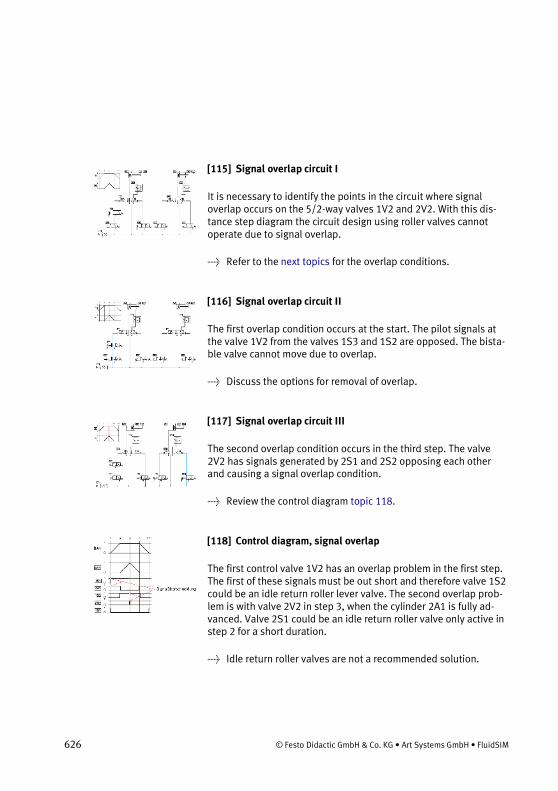
626 © Festo Didactic GmbH & Co. KG • Art Systems GmbH • FluidSIM
[115] Signal overlap circuit I
It is necessary to identify the points in the circuit where signal overlap occurs on the 5/2-way valves 1V2 and 2V2. With this dis-tance step diagram the circuit design using roller valves cannot operate due to signal overlap.
→ Refer to the next topics for the overlap conditions.
[116] Signal overlap circuit II
The first overlap condition occurs at the start. The pilot signals at the valve 1V2 from the valves 1S3 and 1S2 are opposed. The bista-ble valve cannot move due to overlap.
→ Discuss the options for removal of overlap.
[117] Signal overlap circuit III
The second overlap condition occurs in the third step. The valve 2V2 has signals generated by 2S1 and 2S2 opposing each other and causing a signal overlap condition.
→ Review the control diagram topic 118.
[118] Control diagram, signal overlap
The first control valve 1V2 has an overlap problem in the first step. The first of these signals must be out short and therefore valve 1S2 could be an idle return roller lever valve. The second overlap prob-lem is with valve 2V2 in step 3, when the cylinder 2A1 is fully ad-vanced. Valve 2S1 could be an idle return roller valve only active in step 2 for a short duration.
→ Idle return roller valves are not a recommended solution.

© Festo Didactic GmbH & Co. KG • Art Systems GmbH • FluidSIM 627
[119] Idle return roller valve solution
The idle return roller limit switch can be used to remove the signal overlap points, i.e. replace the roller lever limit switches identified, with an idle return roller lever valve. Valves 1S2 and 2S1 generated the signal overlap and therefore these valves should be idle return roller valves.
→ Idle return roller valves are not a recommended solution.
[120] Reversing valve solution
An alternative method of shortening the duration of signals is to remove the air supply to the two signal valves, except at the steps required. Using the reversing valve 1V2, lines S1 and S2 can be activated consecutively and the signals are prevented from over-lapping at the memory valves 1V1 and 2V1.
→ Emphasize the increased reliability of the circuit.
23.10 Educational Films
23.10.1 Educational Films
No. Title Length
1 Introduction 2:42
2 Fundamentals: Structure of hybrid systems 4:32
3 Fundamentals: Fundamentals of electricity 10:26
4 Sensors and relays – Signals 0:48
5 Sensors and relays – Sensors 3:24

628 © Festo Didactic GmbH & Co. KG • Art Systems GmbH • FluidSIM
6 Sensors and relays – Pressure switches 2:41
7 Sensors and relays – Relays 3:34
8 Solenoid valves 2:48
9 Solenoid valves: Double-solenoid valves 1:47
10 Solenoid valves: Pilot control 3:58
11 Pilot control: Circuit-diagram conventions 4:14
12 Pilot control: Hard-wired controllers 4:58
13 Pilot control: Programmable Logic Control-lers
2:25
23.11 Standard Presentations
For several topics useful presentations have been provided within FluidSIM. The following table lists the titles of the predefined presentations.
23.11.1 Presentations
Presentation Title
All topics sorted by number
Basics
Supply elements
Actuators
Directional control valves
Shutoff valves
Flow control valves
Pressure control valves
Time delay valve

© Festo Didactic GmbH & Co. KG • Art Systems GmbH • FluidSIM 629
Sequential circuit and signal overlap circuit
Educational films

Didactics Material Survey (Hydraulics)
630 © Festo Didactic GmbH & Co. KG • Art Systems GmbH • FluidSIM
Chapter 2424. Didactics Material Survey (Hydra ulics)
This chapter provides a comprehensive listing of those parts of the didactics material in FluidSIM that are not covered by chapter The Component Library “The Component Library”. Basically, this mate-rial consists of the components' behavior illustrations, the anima-tions, the exercises, and the educational films, which all can be
activated under the Didactics menu. The subsequent sections
are arranged thematically. The icon indicates that an animation exists for the related topic. The last section gives an overview of the educational films.
24.1 Applications
[1] Lathe
Machine-tool construction is a typical area of application of hydrau-lics. With modern CNC machine tools, the tools and workpieces are clamped by hydraulic means. Feed motions and the spindle drive can also be hydraulically powered.
→ This can also serve as an example of hydraulic circuit with two pressure ranges, for example, 3 MPa (30 bar) for machining and 9 MPa (90 bar) for clamping.
[2] Press with elevated reservoir
This is an application in which extremely high forces are required. Due to the suspended cylinder and the tractive load, special measures are required for the activation of the advance stroke. This in turn requires specially-designed press drives.
→ A special feature is the elevated reservoir, which utilizes the static pressure in the pressure medium.

© Festo Didactic GmbH & Co. KG • Art Systems GmbH • FluidSIM 631
[3] Mobile hydraulics: Excavator
On this hydraulic excavator, not only all working movements (linear drives) but also the propulsion of the vehicle (rotary drive) are hydraulically powered. The primary drive of the excavator is an internal-combustion engine.
→ A model calculation can be used here to demonstrate an ad-vantage of hydraulics - large forces with relatively small com-ponents.
24.2 Components of a Hydraulic Plant
[4] Structure of a hydraulic system
This simplified block diagram shows the division of hydraulic sys-tems into a signal control section and a hydraulic power section. This signal control section is used to activate the valves in the power control section.
→ The material depicted in these electronic slides is concerned in the main with the hydraulic power section and the three “lev-els” of this which are shown.
[5] Hydraulic power section
The diagram of the hydraulic power section is complemented in this case by a circuit diagram to allow correlation of the various function groups; the power supply section contains the hydraulic pump and drive motor and the components for the preparation of the hydrau-lic fluid. The energy control section consists of the various valves used to provide control and regulate the flow rate, pressure and

632 © Festo Didactic GmbH & Co. KG • Art Systems GmbH • FluidSIM
direction of the hydraulic fluid. This drive section consists of cylin-ders or hydraulic motors, depending on the application in question.
[6] Block diagram of a control system
In analyzing and planning an actual control task, it can be helpful to use a differentiated block diagram showing the actual levels to be found on the machine.
→ The light arrows show the signal flow, while the solid dark arrows show the energy flow.
[7] Interaction of components
The animations show the sequences in a basic hydraulic circuit in simplified form - the actuation and spring return of the final control element (4/2-way valve), the advance and return of the drive com-ponent (double acting cylinder) and the opening and closing of the pressure relief valve.
→ The representations of the actuator and final control element are based on the relevant circuit symbols. This can be used as a preparation for the introduction of circuit symbols.
[8] Action related numbering
First of all the control chain is numbered sequentially according to the principle. The first actuator is given the supplementary num-ber.0 and the associated final control element the supplementary number.1. The remaining elements get even numbers if they influ-ence the advance stroke and uneven numbers if they influence the return stroke.
→ The numbering should always be entered in the circuit diagram and also on the machine to enable systematic fault-finding.

© Festo Didactic GmbH & Co. KG • Art Systems GmbH • FluidSIM 633
[9] Numbering in accordance with DIN ISO 1219-2
The DIN ISO Standard 1219-2 defines the code structure of the components as a string consisting of the following four parts: number of the plant, number of the circuit, component designation, and component number. If the entire system consists of a single plant only, the plant number may be dropped.
[10] Numbering in accordance with parts list
Another method used in practice is to number all the components in a hydraulic system consecutively. The numbers then correspond to the numbers in the parts list.
→ This method is used particularly with complex controls sys-tems, for which a control-chain-related numbering system can-not be used due the overlaps involved.
24.3 Symbols
[11] Circuit symbols for energy transfer (1)
The symbols shown are used in circuit diagrams for energy transfer and hydraulic-fluid preparation.
→ In the interests of clarity, the lines in the circuit diagram should be drawn without cross-overs as far as possible.

634 © Festo Didactic GmbH & Co. KG • Art Systems GmbH • FluidSIM
[12] Circuit symbols for energy transfer (2)
The direction of the arrows in the circuit symbols for the heater and cooler correspond to the direction of heat flow.
[13] Circuit symbols for energy conversion
Hydraulic pumps are shown by a circle with a part representation of a drive shaft. Triangles in the circles show the direction of flow. The triangles are shown solid, since pressure fluid is used in hydraulics.
→ If the pressure medium is gaseous, as in the case of pneumat-ics, the triangles are shown in outline.
[14] Circuit symbols for hydraulic motors
The symbols for hydraulic motors are distinguished from the sym-bols for hydraulic pumps by the fact that the arrows showing the direction of flow are the other way round.
[15] Circuit symbols for single acting cylinders
Single acting cylinders have one port, i.e. pressure fluid can be applied only to the piston side. With these cylinders, the return stroke is produced either by external force, shown in the symbol by an opening bearing cap, or by a spring is shown within the symbol in this latter case.
[16] Circuit symbols for double acting cylinders
Double acting cylinders have two ports to allow pressure fluid to be applied to both cylinder chambers. The symbol for a differential cylinder is distinguished from the symbol for a double acting cylin-

© Festo Didactic GmbH & Co. KG • Art Systems GmbH • FluidSIM 635
der by the two lines added to the end of the piston rod. The area ratio is generally 2:1. In the case of cylinders with double- ended piston rods, the symbol shows that the piston areas are of equal size (synchronous cylinders).
[17] Circuit symbols for directional control valves (1)
Designations for directional control valves always give firstly the number of ports and then the number of switching positions. Direc-tional control valves always have at least two ports and at least two switching positions. The number of squares shows the number of possible switching positions of a valve. Arrows within the squares show the direction of flow. Lines shown how the ports are intercon-nected in the various switching positions of the valve. The designa-tions always relate to the normal position of the valve.
[18] Circuit symbols for directional control valves (2)
This illustration shows the circuit symbols for 4/2- and 5/2-way valves.
→ There are two general methods for the designation of ports, using either the letters P, T, R, A, B and L or consecutively using A, B, C, D etc.; the first method is the preferred one in the rele-vant standard.
[19] Circuit symbols for directional control valves (3)
The illustration shows the circuit symbols for 4/3-way valves with various mid-positions.
[20] Circuit symbols for manual operation
The switching position of a directional control valve can be changed by various actuation methods. The symbol for the valve is accord-

636 © Festo Didactic GmbH & Co. KG • Art Systems GmbH • FluidSIM
ingly supplemented by a symbol indicating the actuation methods shown, such as pushbuttons and pedals, a spring is always neces-sary for resetting. Resetting can, however, also be achieved by actuating the valve a second time, for example in the case of valves with hand levers and detents.
→ The various actuating methods possible are listed in DIN ISO 1219.
[21] Circuit symbols for mechanical actuation
This illustration shows the symbols for stem or push button, spring and roller stem.
[22] Circuit symbol for pressure valves
Pressure valves are represented using squares. The flow direction is indicated by an arrow. The valve ports can be designated as P (supply port) and T (tank return port) or as A and B. The position of the arrow within the square indicates whether the valve is normally open or normally closed. Adjustable pressure valves are indicated by a diagonal arrow through the spring. Pressure valves are divided into pressure relief valves and pressure regulators.
[23] Circuit symbols for flow control valves
A distinction is made in flow control valves between types which are affected by viscosity and those which are unaffected. Flow control valves unaffected by viscosity are termed orifices. A 2-way flow control valve consists of restrictors, one adjustable restrictor which is unaffected by viscosity (orifice) and a regulating restrictor (pressure compensator). These valves are represented by a rectan-gle containing the symbol for the adjustable restrictor and an arrow to represent the pressure compensator. The diagonal arrow through the rectangle indicates that the valve is adjustable.

© Festo Didactic GmbH & Co. KG • Art Systems GmbH • FluidSIM 637
[24] Circuit symbols for non-return valves
The symbol for non-return valves is a ball which is pressed against a seat. Delockable non-return valves are shown by a square con-taining the symbol for a non- return valve. The pilot control for unlocking the non- return valve is indicated by a broken line at the pilot port. The pilot port is designated by the letter X.
[25] Circuit symbols for measuring devices
The illustration shows the symbols for measuring devices used in hydraulics.
24.4 Some Physical Fundamentals
[26] Hydrostatic pressure
Hydrostatic pressure is the pressure created above a certain level within a liquid as a result of the weight of the liquid mass. Hydro-static pressure is not dependent on the shape of the vessel con-cerned but only on the height and density of the column of liquid.
→ Hydrostatic pressure can generally be ignored for the purpose of studying hydraulics (exception: see topic 2).
[27] Pressure propagation
If a force F acts on an area A of an enclosed liquid, a pressure p is produced which acts throughout the liquid (Pascal’s Law).

638 © Festo Didactic GmbH & Co. KG • Art Systems GmbH • FluidSIM
→ Hydrostatic pressure has been ignored here. The term pressure propagation is also used to mean the pulse velocity in liquids (approx. 1000 m/s).
[28] Power transmission
If a force F_1 is applied to an area A_1 of a liquid, a pressure p results. If, as in this case, the pressure acts on a larger surface A_2, then a larger counter-force F_2 must be maintained. If A_2 is three times as large as A1, then F_2 will also be three times as large as F_1.
→ Hydraulic power transmission is comparable to the mechanical law of levers.
[29] Displacement transmission (1)
If the input piston of the hydraulic press travels a distance s_1, a volume of fluid will be displaced. This same volume displaces the output piston by the distance s_2. If the area of this piston is larger than that of the input piston, the distance s_2 will be shorter than s_1.
→ Hydraulic displacement transmission is comparable to the mechanical law of levers.
[30] Displacement transmission (2)
See topic 29
[31] Pressure transfer (1)
The fluid pressure p_1 exerts a force F_1 on the surface A_1 which is transferred via the piston rod to the small piston. The force F_1 thus acts on the surface A_2 and produces the fluid pressure p2. Since the piston area A_2 is smaller than the piston area A_1, the pressure p_2 must be larger than the pressure p_1.

© Festo Didactic GmbH & Co. KG • Art Systems GmbH • FluidSIM 639
→ The pressure-transfer (pressure-intensification) effect is put to practical use in pneumatic/hydraulic pressure intensifiers and also in purely hydraulic systems when extremely high pres-sures are required which a pump cannot deliver.
[32] Pressure transfer (2)
A pressure-transfer effect also occurs in conventional double acting cylinders with single piston rod.
→ This effect also causes problems in hydraulics. If, for example, an exhaust flow control is fitted to a differential cylinder for the advance stroke, a pressure- intensification effect results in the piston-rod chamber.
[33] Types of flow
A distinction is made between laminar flow and turbulent flow. In the case of laminar flow, the hydraulic fluid moves through the pipe in ordered cylindrical layers. If the flow velocity of the hydraulic fluid rises above a critical speed, the fluid particles at the center of the pipe break away to the side, and turbulence results.
→ Turbulent flow should be avoided in hydraulic circuits by ensur-ing they are adequate sized.
[34] Diesel effect
A pressure drop to the level of vacuum may occur at points of restriction, causing precipitation of the air dissolved in the oil. When the pressure rises again, oil bursts into the gas bubbles and spontaneous ignition of the oil/air mixture may occur.
[35] Cavitation
Motion energy is required for an increase in the flow velocity of the oil at a restriction. This motion energy is derived from the pressure energy. If the vacuum which results is smaller than -30 kPa (-0.3

640 © Festo Didactic GmbH & Co. KG • Art Systems GmbH • FluidSIM
bar), air dissolved in the oil is precipitated out. When the pressure rises again due to a reduction in speed, the oil bursts into the gas bubbles.
→ Cavitation is a significant factor in hydraulic systems as a cause of wear in devices and connections.
[36] Cavitation
Local pressure peaks occur during cavitation. This causes the erosion of small particles from the wall of the pipe immediately after the reduced cross-section, leading to material fatigue and often also to fractures. This effect is accompanied by considerable noise.
[37] Input and output power
Various losses occur at the individual devices within a hydraulic control chain. These consist essentially of mechanical, electrical and volumetric losses.
→ After an installation has been in service for some time, there will be a change in particular in the volumetric efficiency of the pump, as the result, for example, of cavitation (see topic 35).
24.5 Components of a Power Unit
[38] Hydraulic power unit
The hydraulic power unit (power supply unit) provides the energy required for the hydraulic installation. Its most important compo-nents are the reservoir (tank) , drive (electric motor), hydraulic pump, pressure relief valve (safety valve), filter and cooler. The

© Festo Didactic GmbH & Co. KG • Art Systems GmbH • FluidSIM 641
hydraulic power unit may also act as a carrier for other devices (gauges, directional control valves).
[39] Hydraulic power unit: Reservoir
The hydraulic reservoir contains the hydraulic fluid required the operate the installation. Within the reservoir, air, water and solid matter are separated out of the hydraulic fluid.
→ The size of the reservoir will depend on the practical applica-tion involved; for stationary systems, the volume of fluid deliv-ered by the pump in 3 to 5 minutes can be taken as a guide. In mobile hydraulic systems, on the other hand, the reservoir con-tains only the maximum quantity of hydraulic fluid required.
[40] Externally toothed gear pump
The increase in volume which results when a tooth moves out of mesh produces a vacuum in the suction area. The hydraulic fluid is conveyed into the pressure area. The hydraulic fluid is then forced out of the tooth gaps by the meshing of the teeth and displaced into the above supply line.
[41] Internally toothed gear pump
The inner gear is driven by a motor. The teeth of the inner wheel drive the outer gear wheel. The rotary motion creates a vacuum in the gaps between the teeth, causing hydraulic fluid to be sucked in. On the other side, the teeth engage once more and oil is displaced from the tooth chambers.
→ The design can deliver pressures of up to approx. 17.5 MPa (175 bar). Hydraulic motors represent the reverse of the func-tion principle.

642 © Festo Didactic GmbH & Co. KG • Art Systems GmbH • FluidSIM
[42] Circuit diagram: Return flow filter
An oil filter situated in the return line to the tank has the advantage that the filter is thus easy to maintain. A disadvantage, however, is that contamination is removed from the hydraulic fluid only after it has passed through the hydraulic components.
→ This configuration is often used.
[43] Circuit diagram : Pump inlet filter
With this configuration, the pump is protected from contamination. The filter is, on the other hand, less easily accessible.
→ If these filters have a too fine mesh, suction problems and cavitation effects may occur. Additional coarse filters upstream of the pump are recommended.
[44] Circuit diagram: Pressure line filter
Pressure filters can be installed selectively upstream of valves which are sensitive to contamination; this also enables smaller mesh sizes to be used.
→ A pressure-resistant housing is required, which makes this configuration more expensive.
[45] Circuit diagram: Contamination indicator
It is important that the effectiveness of a filter can be checked by a contamination indicator. The contamination of a filter is measured by the pressure drop; as the contamination increases, the pressure upstream of the filter increases. The pressure acts on a spring- loaded piston. As the pressure increases, the piston is pushed against a spring.

© Festo Didactic GmbH & Co. KG • Art Systems GmbH • FluidSIM 643
→ There are a number of different display methods. Either the piston movement is directly visible or it is converted into an electrical or visual indication by electrical contacts.
[46] Water cooler
With this design of cooler, hydraulic fluid is fed through tubes over which coolant (water) flows. The heat which is discharged can be re-used.
→ The operating temperature in hydraulic installations should not exceed 50 - 60°{C}, since this would cause an unacceptable re-duction in viscosity, leading to premature aging of the fluid. In comparison with air cooling, operating costs a higher due to the required coolant and the susceptibility to corrosion. Tem-perature difference of up to approx. 35°{C} can be handled.
[47] Air cooler
Hydraulic fluid from the return line flows through a coiled pipe which is cooled by a fan.
→ The advantages here are simplicity of installation and low operating costs. The noise of the fan may be a nuisance (see also topic 46).
[48] Heating element
Heaters are often required to ensure that the optimum operating temperature is reached quickly. Heating elements or flow preheat-ers are used for heating and pre-heating hydraulic fluid.
→ If the viscosity is to high, the resulting increase in friction and cavitation leads to greater wear.
[49] Circuit diagram: Hydraulic power unit
The illustration shows the detailed circuit symbol for a hydraulic power unit.

644 © Festo Didactic GmbH & Co. KG • Art Systems GmbH • FluidSIM
→ Since this is an combination unit, a dot/dash line is placed around the symbols representing the individual units.
24.6 Fundamentals of Valves
[50] Actuating force
With some types of poppet valves, the actuating force, which is dependent on pressure and area, may be very high. In order to avoid this, pressure compensation may be provided at the valves.
[51] Poppet principle
Valves are based either on the poppet principle or slide principle. In poppet valves, a ball, a cone or a disc is pressed by a spring against the seat of a passage. The high pressure per unit area which is created, means that valves of this kind provide a very efficient seal. The illustration shows a cone used as a sealing element.
[52] Slide principle
This illustration shows the principle of a longitudinal slide valve. In order to allow the piston to move, it has a certain clearance and floats in hydraulic fluids. Ring grooves ensure an even film of oil and thus pressure equilibrium. The piston can thus be moved with minimal frictional losses.
→ This type of valve cannot provide a perfect seal, which means that there is always a certain oil leakage.

© Festo Didactic GmbH & Co. KG • Art Systems GmbH • FluidSIM 645
[53] Poppet valves
In poppet valves, a ball, cone or occasionally a disk is pressed against a seat area to act as a sealing element. Valves of this type provide a very efficient seal.
[54] Piston overlap
The switching characteristics of a valve are governed by, among other things, its piston overlap. A distinction is made between positive, negative and zero overlap. In the case of positive overlap, the port in question is completely covered by the piston, while with negative overlap it is less than completely covered. In the case of zero overlap, the distances between the control edges of the piston and of the port are exactly the same.
→ The individual control edges of the pilot piston can have differ-ent overlaps.
[55] Negative switching overlap
In the case of negative overlap, flow from A to T is not quite closed when the inlet P is opened. This means that the pressure at port A rises slowly and the piston starts gently.
→ In manufacturers' data sheets, overlap positions are shown within dotted lines between the switching positions, or the overlap positions are shown in color or with a patterned back-ground.
[56] Positive switching overlap
In the case of positive overlap, the left-hand piston does not open the passage from P to A until the tank has been completely isolated by the other piston. Pressure is immediately fed to the load device (cylinder or hydraulic motor) with the result that this starts abrupt-ly.

646 © Festo Didactic GmbH & Co. KG • Art Systems GmbH • FluidSIM
[57] Control edges
The control edges of the pistons are often either sharp, chamfered or notched. The profiling of the control edges means that the throt-tling action of the flow when switching is gradual rather than ab-rupt.
→ See also the example in topic 144.
[58] Vertical interconnection system
Vertical interconnection systems (“modular hydraulics”) mean that less space is required and that no piping is needed between the components. The circuit symbols directly marked on the compo-nents give greater clarity in the installation.
24.7 Pressure Valves
[59] Pressure relief valve (1)
In this design incorporating a poppet valve, a seal is pressed against the inlet port P by a pressure spring when the valve is in its normal position.
→ In this situation, for example, an unloaded piston rod is execut-ing an advance stroke and the entire pump delivery is flowing to the cylinder.
[60] Pressure relief valve (2)
As soon as the force exerted by the inlet pressure at A exceeds the opposing spring force, the valve begins to open.

© Festo Didactic GmbH & Co. KG • Art Systems GmbH • FluidSIM 647
→ In this situation, for example, the piston rod is fully advanced; the entire pump delivery is flowing at the preset system pres-sure to the tank.
[61] PRV used to limit system pressure
This illustration shows a pressure relief valve within a basic hydrau-lic circuit (used to control a double acting cylinder).
→ The resistances at the outlet (tank line, filter) must be added to the force of the spring in the pressure relief valve. See also the animation “Interaction of components” (topic 7).
[62] Circuit diagram: PRV used to limit system pressure
This illustration shows the same circuit as the previous illustration, but with the cut-away view of the PRV replaced by the appropriate circuit symbol.
[63] Circuit without brake valve
One application of pressure relief valves is as brake valves; these prevent pressure peaks which may otherwise occur as the result of mass moments of inertia when a directional control valve is sud-denly closed. The animation shows an (incorrect) circuit in schemat-ic form in which the working line on the exhaust side has fractured due to the absence of a brake valve.
→ The next animation (topic 64) shows the correct circuit.
[64] Circuit diagram: Brake valve
This illustration shows the correct circuit for the problem in topic 63. This circuit incorporates not only a brake valve on the piston-rod side but also a non-return valve on the inlet side via which oil can be taken in from a reservoir during the vacuum phase following the closure of the directional control valve.

648 © Festo Didactic GmbH & Co. KG • Art Systems GmbH • FluidSIM
→ The following animation shows the events which occur in the two working lines.
[65] Circuit with brake valve
First the animation shows in schematic form the behavior of the PRV during the braking phase, then it shows the behavior of the non-return valve (NRV) in the supply line.
→ The necessity of the brake valve can be demonstrated by topic 63.
[66] Circuit diagram: PRV as back-pressure valve
Back-pressure valves counteract mass moments of inertia with tractive loads. The illustration shows a circuit with a back-pressure valve on the piston-rod side. On the return stroke, the PRV is by-passed by an NRV.
→ The PRV must be pressure-compensated and the tank port must be capable of carrying a pressure load.
[67] PRV, internally controlled, cushioned
Pressure relief valves often incorporate cushioning pistons or flow control valves. The cushioning device shown provides fast opening and slow closing of the valve. This prevents damage caused by pressure shocks (smooth valve operation).
→ Pressure shock arise, for example, when the pump delivers oil in an almost unpressurized condition and the supply port of the load device is abruptly closed by a directional control valve.
[68] PRV, externally controlled (1)
This pressure relief valve controls the flow in accordance with an external pressure setting. This pressure acts against an adjustable

© Festo Didactic GmbH & Co. KG • Art Systems GmbH • FluidSIM 649
spring force. The passage from the supply port P to the tank port T remains closed as long as no load acts on the pilot piston.
[69] PRV, externally controlled (2)
Pressure can be fed to the pilot piston via the pilot port X. As soon as the pressure force at the pilot piston exceeds the preset spring force, the pilot piston is displaced, allowing free flow.
[70] Sequence valve
The example shows a circuit with a pressure relief valve used as a pressure sequence valve. The pressure at the pilot piston of the PRV rises via the pressure regulator. The PRV opens and the high-pressure pump delivers directly to the tank. As soon as the 2/2-way valve opens, the pressure drops. The pressure relief valve closes and the high pressure pump is connected to the system.
[71] Circuit diagram: Sequence valve
This illustration shows the same circuit as the previous illustration, but with the cut-away view of the sequence valve replaced by the appropriate circuit symbol.
[72] Pressure relief valve
Actual photograph of a pressure relief valve.
[73] 2-way pressure regulator (1)

650 © Festo Didactic GmbH & Co. KG • Art Systems GmbH • FluidSIM
This valve is normally open. The outlet pressure (A) acts via a pilot line on the left-hand surface of the pilot piston against an adjusta-ble spring force.
→ Pressure regulators reduce the inlet pressure to an adjustable outlet pressure. It is appropriate to use these in hydraulic in-stallations only if different pressures are required.
[74] 2-way pressure regulator (2)
When the pressure rises at outlet A, the force at the left-hand surface of the pilot piston becomes greater, the piston is displaced to the right and the throttle gap becomes narrower. This causes a pressure drop.
→ In the case of slide valves, it is also possible to design the control edges in such way that the opening gap increases only slowly. This gives greater control precision.
[75] 2-way pressure regulator (3)
When the preset maximum pressure is reached, the throttle point closes completely; the pressure set on the pressure relief valve is produced at the inlet P.
[76] 2-way pressure regulator (4)
In the circuit illustrated, the piston rod of the cylinder is executing an advance stroke. The pressure at the outlet A of the pressure regulator is less than the system pressure at P and constant.
[77] 2-way pressure regulator (5)
The piston rod of the cylinder is now in its forward end position. The pressure at outlet A thus continues to rise and the throttle point closes completely.

© Festo Didactic GmbH & Co. KG • Art Systems GmbH • FluidSIM 651
[78] Circuit diagram: 2-way pressure regulator
The illustration shows the same circuit as the previous illustration, but with the 2-way pressure regulator in the form of a circuit sym-bol.
[79] Circuit diagram: 2-way pressure regulator
It is appropriate to use PRVs only when different pressures are required in an installation. The mode of operation of pressure regulator will thus be explained here by taking an example with two control circuits. The first control circuit acts via a flow control valve on a hydraulic motor which drives a roller. This roller is used to stick together multi-layered printed circuit boards. The second control circuit acts on a hydraulic cylinder which draws the roller towards the boards at an adjustable reduced pressure.
→ This example can be used as a preliminary stage to the intro-duction of the 3-way PR. If the 2-way PR is closed due to the fact that the preset maximum pressure has been reached, thickening of the material of the workpieces would cause an in-crease in the pressure on the outlet side of the PR to a higher value than desired. (See also the animation for topic 84.)
[80] 3-way pressure regulator (1)
The 3-way pressure regulator can be regarded as a combination of a 2-way PR and a pressure relief valve (PRV). The PR is in its normal position here; only a low pressure has built up at the outlet A.
[81] 3-way pressure regulator (2)
When the pressure at A rises the result of external conditions, this pressure acts via a pilot line on the left-hand piston surface of the pilot piston against an adjustable spring force. Every pressure

652 © Festo Didactic GmbH & Co. KG • Art Systems GmbH • FluidSIM
increase causes the throttle gap to become narrower, resulting in a pressure drop.
[82] 3-way pressure regulator (3)
When the maximum preset pressure is reached, the throttle point closes completely. The pressure set on the system-pressure limiter is produced at the inlet P.
[83] 3-way pressure regulator (4)
If the pressure rises above the preset value as the result of an external load at outlet A, the valve opens to allow flow from A to the tank port T (pressure-limiter function).
→ 3-way pressure regulators are available with both positive and negative piston overlap. If a 3-way pressure regulator is creat-ed by combining a 2-way pressure regulator and a pressure re-lief valve, the “overlap” is adjustable.
[84] 3-way pressure regulator
The animation shows both the pressure-regulator and pressure-limiter function of a 3-way pressure regulator through the example of a roller which exerts a constant pressure on moving material of variable thickness.
→ The final control element which is normally interposed has been omitted here in the interests of clarity.
[85] 3-way pressure regulator (5)
A 3-way PR is shown here in a functional representation, incorpo-rated into a model circuit diagram. The piston rod of the cylinder is subject to external force and the pressure regulator provides a pressure-limiter function.

© Festo Didactic GmbH & Co. KG • Art Systems GmbH • FluidSIM 653
[86] 3-way pressure regulator (6)
The illustration shows the same circuit as the previous illustration, but with the functional representation of the 3-way pressure regu-lator replaced by a “detailed” circuit symbol.
→ 3-way pressure regulators are available with both positive and negative piston overlap. If a 3-way pressure regulator is creat-ed by combining a 2-way pressure regulator and a pressure re-lief valve, the “overlap” is adjustable.
[87] Circuit diagram: 3-way pressure regulator
The illustration shows the same circuit as the previous illustration, but with the standard circuit symbol for a 3-way pressure regulator.
24.8 Way Valves
[88] 2/2-way valve (1)
The 2/2-way valve has a working port A, a supply port P and a leakage-oil port L. In the case of the valve shown here, of slide design, flow from P to A is closed in the normal position.
→ A relief line leading to the leakage-oil port is provided to pre-vent a build-up of pressure in the spring and piston chambers.
[89] 2/2-way valve (2)
The 2/2-way valve is actuated and the passage from P to A is open.
→ 2/2-way valves are also available which are normally open from P to A.

654 © Festo Didactic GmbH & Co. KG • Art Systems GmbH • FluidSIM
[90] 2/2-way valve as by-pass valve
This example shows a 2/2-way valve used as a by-pass valve; when the 2/2-way valve is actuated, the flow control valve 0V2 is by-passed, causing the piston rod of the cylinder to advance at maxi-mum speed.
[91] Circuit diagram: 2/2-way valve as by-pass valve
The illustration shows the same circuit as the previous illustration, but with the functional representation of the 2/2-way valve re-placed by a circuit symbol.
[92] Circuit diagram: 2/2-way valve as final control element
In its initial position, the cylinder is advanced. If the 2/2- way valve 0V1 is actuated, the entire volumetric flow passes to the tank and piston rod of the cylinder is reset by the external load m. If 0V1 is not actuated, the system pressure set on the pressure limiter 0V2 builds up and the piston rod advances.
→ In the initial position, the pump operates against the preset system pressure, which has an unfavorable effect on the power balance of the circuit shown.
[93] 2/2-way valve as final control element
The animations show the actuation and release of the 2/2-way valve, which causes the piston rod of the cylinder to advance and retract.

© Festo Didactic GmbH & Co. KG • Art Systems GmbH • FluidSIM 655
[94] Circuit diagram for pressure-less pump recirculation
The part circuit diagram shows a 2/2-way valve used as a by-pass valve to achieve pressure-less pump recirculation; if the valve is actuated, the pump no longer needs to operate against the preset system pressure.
→ One application of this circuit is with 4/3-way valves which are closed in their mid-position in cases where, with the installa-tion operational, it is desired to switch to pump recirculation (see also topic 116).
[95] Circuit diagram: Pressure stage circuit
The part circuit diagram shows a 2/2-way valve used as a selector switch for one of two preset system pressures (“pressure levels”); if the 2/2-way valve is actuated, flow is enabled to a second sys-tem-pressure limiter.
[96] 3/2-way valve (poppet principle) (1)
The 3/2-way valve has working port A, a supply port P and a tank port T. Volumetric flow can be routed from the supply port to the working port or from the working port to the tank port. The third port in each case is closed. In the normal position shown, P is closed and flow released from A to T.
→ See also topic 101 (slide principle).
[97] 3/2-way valve (poppet principle) (2)
The 3/2-way valve is actuated; flow is released from P to A, the outlet T is closed.
→ 3/2-way valves which are normally open from P to A and T closed are also available.

656 © Festo Didactic GmbH & Co. KG • Art Systems GmbH • FluidSIM
[98] 3/2-way valve as final control element
The circuit shows the 3/2-way valve in a functional representation as a final control element of a single acting cylinder.
→ The non-return valve protects the pump in cases where the 3/2-way valve is actuated and the piston rod is subject to an external load.
[99] Circuit diagram: 3/2-way valve as final control element
The illustration shows the same circuit as the previous illustration, but with the circuit symbol for the 3/2-way valve.
[100] 3/2-way valve
The animations show the actuation and release of the manual pushbutton for a 3/2-way valve, which causes the piston rod of the cylinder to advance and retract.
[101] 3/2-way valve (slide principle) (1)
The 3/2-way valve has a working port A, a supply port P and a tank port T. The volumetric flow can be routed from the supply port to the working port, or from the working port to the tank port. The third port in each case is closed. In the normal position shown, P is closed and flow is released from A to T.
→ See also the 3/2-way valve designed on the poppet principle (Topic 96).

© Festo Didactic GmbH & Co. KG • Art Systems GmbH • FluidSIM 657
[102] 3/2-way valve (slide principle) (2)
The 3/2-way valve is actuated; flow is released from P to A, and the outlet T is closed.
→ 3/2-way valves which are normally closed from P to A and T are also available.
[103] 3/2-way valves as diverter
In addition to their application as final control elements, 3/2-way valves can also be used as diverters. In this case, port T is connect-ed to a further device, to which a switch-over can then be made. The part circuit diagrams show the facility to switch between the flow control valves with different settings and between heating and cooling.
→ The circuit symbol is drawn reversed to simplify the representa-tion of the circuit diagram.
[104] 4/2-way valve, two pistons (1)
The 4/2-way valve has two working ports A and B, a supply port P and a tank port T. The supply port is always connected to one of the working ports, while the second working port is routed to the tank. In the normal position, there is flow from P to B and from A to T.
→ In contrast to valves with three pistons, 4/2-way valves with two pistons do not require a leakage-oil port (see topic 106).
[105] 4/2-way valve, two pistons (2)
The 4/2-way valve is actuated, and there is flow from P to A and from B to T.
→ 4/2-way valves are also available which are normally open from P to A and from B to T.

658 © Festo Didactic GmbH & Co. KG • Art Systems GmbH • FluidSIM
[106] 4/2-way valve, three pistons (1)
This 4/2-way valve has two working ports A and B, a supply port P and a tank port T. The supply port is always connected to one of the working ports, while the second working port is routed to the tank. In the neutral position, there is flow from P to B and from A to T.
→ 4/2-way valves with three pistons require a leakage-oil port, since hydraulic fluid would otherwise be trapped within the valve.
[107] 4/2-way valve, three pistons (2)
The 4/2-way valve is actuated, and there is flow from P to A and from B to T.
[108] 4/2-way valve, three pistons (3)
The circuit shows the 4/2-way valve in functional representation as a final control element of a double acting cylinder.
→ The non-return valve protects the pump in cases where the piston rod of the cylinder is subject to an external load.
[109] Circuit diagram: 4/2-way valve
The illustration shows the same circuit as the previous illustration, but with the 4/2-way valve as a circuit symbol.
[110] 4/3-way valve with pump bypass (1)
From the logic point of view, 4/3-way valves are 4/2- way valves with an additional mid-position. There are various versions of this mid-position (in the mid-position in the example shown, the supply

© Festo Didactic GmbH & Co. KG • Art Systems GmbH • FluidSIM 659
port P is directly connected to the tank T, see next illustration). In the switching position shown, there is flow from P to B and from A to T.
→ 4/3-way valves are easy to construct as slide valves and of complex design as poppet valves.
[111] 4/3-way valve with pump bypass (2)
The 4/3-way valve is in its mid-position; there is flow from P to T, while A and B are closed. Since the output from the pump flows to the tank, this switching position is called pump bypass or also pump recirculation.
→ In the case of pump bypass, the pump needs to operate only against the resistance of the valve, which has a favorable effect on the power balance.
[112] 4/3-way valve with pump bypass (3)
The valve is in its left-hand switching position; there is flow from P to A and from B to T.
[113] 4/3-way valve with pump bypass (4)
The circuit shows the 4/3-way valve in functional representation as a final control element of a double acting cylinder. The valve is in its mid-position; the pump delivery flows via the by-pass line within the pilot piston to the tank.
→ The non-return valve protects the pump in cases where the piston rod of the cylinder is subject to an external load.
[114] Circuit diagram: 4/3-way valve with pump bypass
The illustration shows the same circuit as the previous illustration, but with the 4/3-way valve as a circuit symbol.

660 © Festo Didactic GmbH & Co. KG • Art Systems GmbH • FluidSIM
[115] 4/3-way valve with pump bypass
The animations show the switching of the 4/3-way valve into the three switching positions and the corresponding cylinder move-ments. During the advance stroke, movement can be halted by switching to the mid- position.
→ As appropriate to the application in question, a circuit of this kind must be equipped with a brake valve to prevent damage to the installation when the valve is switched to the mid-position (see also topic 64).
[116] 4/3-way valve with closed mid-position (1)
From the logic point of view, 4/3-way valves are 4/2- way valves with an additional mid-position. There are various versions of this mid-position (in the mid-position in the example shown, all ports are closed in the mid- position, see next illustration). In the switch-ing position shown, there is flow from P to B and from A to T.
[117] 4/3-way valve with closed mid-position (2)
The 4/3-way valve is in its mid-position; all ports apart from the leakage-oil port are closed.
→ In this mid-position, the pump is operating against the system pressure set on the pressure relief valve.
[118] 4/3-way valve with closed mid-position (3)
The valve is in its left-hand switching position; there is flow from P to A and from B to T.

© Festo Didactic GmbH & Co. KG • Art Systems GmbH • FluidSIM 661
[119] 4/3-way valve with closed mid-position (4)
The circuit shows the 4/3-way valve in functional representation as a final control element of a double acting cylinder. The valve is in its mid-position; the pump is operating against the system pressure set on the PRV.
→ If, with an operational installation, it is desired to switch to pump recirculation, this can be achieved by using an additional 2/2-way valve as a changeover valve (see part circuit-diagram in topic 94).
[120] Circuit diagram: 4/3-way valve with closed mid-position
The illustration shows the same circuit as the previous illustration, but with the 4/3-way valve as a circuit symbol.
[121] 4/3-way valve: overlap positions (1)
The illustration shows the left-hand overlap position of a 4/3-way valve with positive overlap in the mid-position (closed mid-position). This overlap position is a mixture of positive and negative overlap; P is connected to A, B and T are closed.
→ With 4/3-way valves, the types of overlap positions is generally specified in the data sheet.
[122] 4/3-way valve: overlap positions (2)
The illustration shows the “right-hand” overlap position of a 4/3-way valve with positive overlap in the mid- position (closed mid-position). This overlap position, too, is a mixture of positive and negative overlap; P is connected to B, A and T are closed.

662 © Festo Didactic GmbH & Co. KG • Art Systems GmbH • FluidSIM
[123] Way valve
Actual photograph of a directional control valve with lever actua-tion.
[124] 4/3-way module
This 4/3-way module with hand-lever actuation is used in vertical interconnection systems (“modular hydraulics”).
→ See also the illustration in topic 58.
24.9 Shutoff Valves
[125] Non-return valve (1)
Non-return valves block flow in one direction and allow free flow in the other. In the direction of flow shown, the sealing element is pressed against a seat by a spring and the hydraulic fluid.
→ These valves are also available in designs without springs. Since there must be no leaks in the closed position, these valves are generally of poppet design.
[126] Non-return valve (2)
In the direction of flow shown, the valve is opened by the hydraulic fluid, which lifts the sealing element from the seat.

© Festo Didactic GmbH & Co. KG • Art Systems GmbH • FluidSIM 663
[127] Circuit diagram: Pump protection
In this circuit, the non-return valve is used to protect the pump. This prevents a load pressure from driving the pump in reverse when the electric motor is switched off. Pressure peaks do not affect the pump but are discharged via the pressure relief valve.
[128] Graetz block (1)
In the Graetz rectifier circuit (Graetz block), four non- return valves are combined to form a function unit. The circuit diagram shows how this operates in conjunction with a flow control valve; flow passes through this valve from left to right during both the advance and return strokes of the cylinder. The situation during the advance stroke is shown.
→ During the advance stroke shown here, flow control is carried out on the inlet side.
[129] Graetz block (2)
The cylinder is on its return stroke. The rectifier circuit means that flow once again passes through the flow control valve from left to right.
→ During the return stroke shown here, flow control is carried out on the outlet side.
[130] Graetz block
The animation shows the actuation and spring return of a 4/2-way valve and the flow through the Graetz block during the advance and return strokes.
→ Similar rectifier circuits are also used in conjunction with line filters or brake valves.
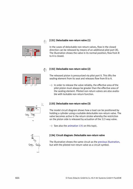
664 © Festo Didactic GmbH & Co. KG • Art Systems GmbH • FluidSIM
[131] Delockable non-return valve (1)
In the cases of delockable non-return valves, flow in the closed direction can be released by means of an additional pilot port (X). The illustration shows the valve in its normal position; flow from B to A is closed.
[132] Delockable non-return valve (2)
The released piston is pressurized via pilot port X. This lifts the sealing element from its seat and releases flow from B to A.
→ In order to release the valve reliably, the effective area of the pilot piston must always be greater than the effective area of the sealing element. Piloted non-return valves are also availa-ble with lockable non-return function.
[133] Delockable non-return valve (3)
The model circuit diagram shows how a load can be positioned by holding a cylinder using a suitable delockable non-return valve. The valve becomes active in the return stroke whereby the restriction on the piston side is released by actuation of the 3/2-way valve.
→ See also the animation 135 on this topic.
[134] Circuit diagram: Delockable non-return valve
The illustration shows the same circuit as the previous illustration, but with the piloted non-return valve as a circuit symbol.

© Festo Didactic GmbH & Co. KG • Art Systems GmbH • FluidSIM 665
[135] Delockable non-return valve
The 4/2-way valve is actuated, the hydraulic fluid passes through the non-return valve against the force of the return spring and the piston rod advances. When the 4/2-way valve is reset, the outlet on the piston side is closed by the non-return valve, and the cylinder remains advanced. The 3/2-way valve is now actuated, the pilot piston is reversed and the outlet flow released; the piston rod begins to retract. During the return stroke, the 3/2-way valve is brought temporarily into its normal position. This causes the outlet to be closed again, and the piston rod and load remain in their current position. When the 3/2-way valve is actuated again, the piston rod travels to its retracted end position.
[136] Delockable double non-return valve (1)
Delockable double non-return valves allow a load to be positioned reliably with the cylinder at a standstill, even if eternal leaks exist around the cylinder piston. When, as in the case, neither of the inlets A_1 or A_2 is pressurized, B_1 and B_2 are closed.
[137] Delockable double non-return valve (2)
When A_1 is pressurized, the left-hand sealing element is lifted from its seat, enabling flow to B_1. At the same time, the pilot piston is displaced to the right, releasing flow from B_2 to A_2.
→ The opposite is true when inlet A_2 is pressurized.
[138] Delockable double non-return valve (3)
The model circuit diagram shows a delockable double non-return valve used in conjunction with a 4/3-way valve to allow the vertical positioning of a load. In the mid-position of the final control ele-ment shown, ports A and B are connected to the tank. This means

666 © Festo Didactic GmbH & Co. KG • Art Systems GmbH • FluidSIM
that the inlets A_1 and A_2 of the double non-return valve are pressure-less and both cylinder supply lines are closed.
[139] Circuit diagram: Delockable double non-return valve
The illustration shows the same circuit as the previous illustration, but with the delockable double non-return valve as a circuit sym-bol.
24.10 Flow Valves
[140] Needle restrictor
Throttle and orifice valves are used to achieve a certain pressure drop. This is done by creating a specific flow resistance. The needle flow control valve shown generates considerable friction due to its long narrowing. This means that the action of the flow control valve is difficult to adjust due to the fact that a small adjustment produc-es a large change in cross-section.
→ One advantage is the simple and inexpensive design. Needle flow control valves can be used if the above- mentioned nega-tive properties can be ignored for the purposes of a given con-trol task.
[141] Gap restrictor with helix
Its short narrowing means that the action of this gap flow control valve is virtually independent of viscosity. The helix provides pre-cise adjustability, since adjustment from fully open to fully closed requires a 360° turn. The helix is, however, very costly to produce.

© Festo Didactic GmbH & Co. KG • Art Systems GmbH • FluidSIM 667
[142] Circuit diagram: Flow division using restrictor
Throttle and orifice valves control the volumetric flow rate in con-junction with a pressure relief valve. The PRV opens when the resistance of the flow control valve becomes greater than that of the opening pressure set on the PRV. This produces a division of flow.
→ The volumetric flow to the load device varies, i.e. the action of flow control valves is load-dependent.
[143] Throttle valve
Actual photograph of a flow control valve.
[144] One-way flow control valve (1)
The one-way flow control valve is a combination of an orifice or throttle valve and a non-return valve. In the closed direction shown of the non-return valve, the volumetric flow passes via the variable throttle gap, which creates a considerable resistance.
→ Speed reduction can be achieved by using a one-way flow control valve in conjunction with a pressure relief valve or a variable-delivery pump. The pressure rises upstream of the flow control valve until the PRV opens and routes part of the flow to the tank.
[145] One-way flow control valve (2)
In the reverse direction, from B to A, flow is unrestricted, since the ball in the one-way flow control valve allows free flow (non-return function).
→ One-way flow control valves are available with a fixed restrictor and with variable flow control.

668 © Festo Didactic GmbH & Co. KG • Art Systems GmbH • FluidSIM
[146] 2-way flow control valve (1)
Flow control valves have the task of providing constant volumetric flow independently of pressure changes at the inlet or outlet of the valve. This is achieved firstly by means of an adjustable restrictor which is set to the desired volumetric flow. In order to keep the pressure drop across the throttle point constant, a second regulat-ing restrictor (pressure compensator) is also required. The illustra-tion shows the valve in its normal position.
→ 2-way flow control valves always operate in conjunction with a pressure relief valve. The part of the flow which is not required is discharged via the PRV.
[147] 2-way flow control valve (2)
When fluid flows through the valve, the pressure drop across the adjustable restrictor is kept constant by the pressure compensator, which varies the resistance at the upper throttle point in accord-ance with the load at the inlet or outlet.
→ See also the animation 150 for this topic.
[148] 2-way flow control valve (3)
In the case of this flow control valve, the pressure difference is kept constant by a adjustable restrictor, i.e. between p_1 and p_2. If the pressure p_3 rises as the result of an external load, the overall resistance of the valve is reduced by opening the regulating restric-tor.
[149] Circuit diagram: 2-way flow control valve
The model circuit diagram shows the arrangement of a 2-way flow control valve in the piston-side supply line in order to achieve a constant feed speed even under varying load. A non-return valve is

© Festo Didactic GmbH & Co. KG • Art Systems GmbH • FluidSIM 669
fitted in the by-pass to allow the flow control valve to be by-passed on the return stroke.
[150] 2-way flow control valve
The advancing piston rod encounters a load half-way through its stroke. The flow control valve nonetheless ensures that the ad-vance speed remains constant. From 0 to 2 seconds (shown at bottom right) the piston rod is unloaded and the pressure condi-tions remain constant. When the piston rod encounters the load, the pressure p_3 rises at the outlet of the flow control valve. (In order to allow the rapid control operations to be shown more clear-ly, the time scale now changes to 1/100ths of a second.) The flow control valve briefly raises the pressure p_2 downstream of the adjustable restrictor. Following this, the regulating restrictor moves to the left, and p_2 falls back to its original value, i.e. the pressure difference between p_1 and p_2 remains constant. The regulating operation shown is repeated a number of times, as the result of which p_3 increases to 2.5 MPa (25 bar) in several steps and the regulating restrictor opens more and more. (At the point at which 2.5 MPa (25 bar) is reached, the time scale changes back to 0.1 seconds.) The piston rod now travels under load just as fast as previously without load.
24.11 Hydraulic Cylinders and Motors
[151] Single acting cylinder
In the case of a single acting cylinder, only the piston side is pres-surized with hydraulic fluid. The cylinder can thus carry out work only in one direction. The fluid which flows into the piston chamber causes a pressure to build up the surface of the piston. The piston travels into its forward end position. The return stroke is effected by a spring, the dead weight of the piston rod or an external load.

670 © Festo Didactic GmbH & Co. KG • Art Systems GmbH • FluidSIM
[152] Plunger cylinder
In the case of plunger cylinders, the piston and rod form a single component. Due to the design of the cylinder, the return stroke can only be effected by external forces. The cylinders can therefore generally be installed only vertically.
[153] Double acting cylinder
In the case of double acting cylinders, both piston surfaces can be pressurized. A working movement can thus be performed in both directions.
→ With double acting cylinders with a single-sided piston rod, different forces and speeds are obtained on the advance and return strokes due to the difference in area between the piston surface and annular piston surface.
[154] Double acting cylinder with end position cushioning
Cylinder with end position cushioning are used to brake high stroke speeds smoothly and prevent hard impacts at the end of the stroke. Shortly before the end position is reached, the cross- section for the outflow of fluid is reduced by the built-in cushioning pistons and then finally closed. The hydraulic fluid is then forced to escape through a flow control valve.
[155] End position cushioning (1)
The piston is a short distance before its end position; the hydraulic fluid on the piston-rod side must escape via the adjustable flow control valve above the piston rod

© Festo Didactic GmbH & Co. KG • Art Systems GmbH • FluidSIM 671
→ This type of end position cushioning is used for stroke speed between 6 m/min and 20 m/min. At higher speed, additional cushioning or braking devices must be used.
[156] End position cushioning (2)
The piston rod is on its return stroke; in this flow direction, the non-return valve below the piston rod is opened, thus by-passing the flow control valve. The piston rod retracts at maximum speed.
[157] End position cushioning
The illustration shows first the advance of the piston rod from a mid-position to the forward end position, with cushioning at the end of the advance movement. The non-return valve is open during the return stroke.
→ In addition the animation shows the opening of the pressure limiter after a certain pressure has been built up on the outlet side by the cushioning piston.
[158] Double acting cylinder
Actual photograph of a double acting cylinder.
[159] Automatic bleed valve
When the cylinder is retracted, the piston of the bleed valve is closed. It is lifted as the piston rod advances. Air can then escape via the bleed hole until the hydraulic fluid reaches the piston and pushes it upwards. In the forward end position, the piston is pushed fully upwards by the hydraulic fluid and thus provides an external seal.
→ Bleed valves should be fitted at the highest point in a piping system, since this is where any trapped air will collect.

672 © Festo Didactic GmbH & Co. KG • Art Systems GmbH • FluidSIM
24.12 Gauges
[160] Piston pressure gauge
Pressure gauges operate on the principle that pressure acting on a given area will produce a given force. In the case of piston pressure gauges, the pressure acts on a piston against the force of a spring. The pressure value is now shown on a scale either by the piston itself or by a pointer driven magnetically by the piston.
[161] Bourdon-tube pressure gauge
Most pressure gauges operate on the principle of a Bourdon tube. When hydraulic fluid flows into the tube, an identical pressure is produced throughout. Due to the difference in area between the outer and inner curved surfaces, the tube is bent. This movement is transferred to a pointer.
→ This type of gauge is not protected against overload. A cush-ioning restrictor must be installed in the inlet connection pre-vent pressure surges from damaging the tube.
[162] Flow meter
The flow of oil to be measured passes through a movable orifice. The orifice consists of a fixed cone and a hollow piston mounted on a spring. The piston is pressed against the spring in proportion to the flow rate concerned. The measuring error of this type of flow meter is approx. 4%. Measuring turbines, oval disk meters or toothed-wheel gauges are used when higher accuracy is required.

© Festo Didactic GmbH & Co. KG • Art Systems GmbH • FluidSIM 673
24.13 Exercises
[163] Exercise: Horizontal grinding machine (pump delivery)
The slide on a horizontal grinding machine is hydraulically actuat-ed. A machine operator determines that the reciprocating move-ment of the machine is no longer reaching the desired speed. A possible cause of this is reduced pump delivery. To investigate this, it is necessary to plot a characteristic curve for the pump and com-pare this with the values achieved during initial commissioning. As an additional exercise, the circuit diagram and parts list for the necessary test assembly should be prepared.
In order to draw the characteristic curve for the pump, the volu-metric flow of hydraulic fluid delivered by the pump (Q) is plotted against the operating pressure achieved (p). The manufacturer’s characteristic curve exhibits a slight downward gradient, since the new pump manifests increasing internal leakage losses as neces-sary to provide internal lubrication. The newly-plotted curve shows a clear deviation; the leakage oil losses have become greater at higher operating pressures, the volumetric efficiency has become worse. The main reason for this is pump wear. Regarding the circuit diagram for the test assembly: The adjustable flow control valve 1V3 is adjusted in such a way that the pressure gauge 1Z1 shows the desired system pressure. The pressure relief valve 1V2 is used to limit the system pressure, while valve 1V1 acts as a safety valve for the pump.
→ The measured values taken as the basis for this exercise do not allow for the characteristic curve of the electric motor. The mo-tor characteristic thus forms part of the calculated error.

674 © Festo Didactic GmbH & Co. KG • Art Systems GmbH • FluidSIM
[164] Exercise: Bending machine (directly-controlled pressure relief valve)
A bending machine is used to bend steel plates. The bending tools are driven by hydraulic cylinders. It is now desired to use the bend-ing machine for considerably thicker steel plates than before. This requires a hydraulic system pressure of 45 bar against the previous 30 bar. According to the manufacturer’s data, the pump used is suitable for the higher operating pressure. Testing reveals, howev-er, that the bending process is now much too slow. In this case, leakage losses in the piping or directional control valve are ruled out as the cause of the problem. A directly-controlled pressure relief valve (PRV) is installed as a safety valve. Measurements of the volumetric flow (Q) as a function of pressure (p) are available for this valve. A characteristic curve can then be used to determine whether the loss of speed in the bending process is due to the PRV.
The volumetric flow which is discharged to the tank when the PRV opens is entered on the horizontal axis. The characteristic curve shows that the opening point of the PRV is 44 bar, although it is set to 50 bar. This means that part of the pump delivery is diverted at pressures greater than 44 bar. Pressures of more than 44 bar are achieved during the bending process. Since, however, the flow is divided from 44 bar onwards, the volumetric flow to the cylinder is reduced from this point and the bending process slows down. Measure to be taken: The PRTV can be set to 60 bar if the overall installation has been designed for this higher pressure. Flow diver-sion will then take place from a pressure of 54 bar onwards.
→ An alternative solution would be to use a valve with a different response pressure.
[165] Exercise: Roller conveyor (flow resistance)
Steel blocks are transported on a roller conveyor. A hydraulic transfer station makes it possible to transfer blocks from one track

© Festo Didactic GmbH & Co. KG • Art Systems GmbH • FluidSIM 675
to another. A pressure of at least 30 bar is required for the transfer of blocks by means of hydraulic cylinders. Every component through which the hydraulic fluid flows represents a resistance and causes a constant pressure loss. The question is, what pressure is to be set at the pressure relief valve.
The total resistance is the sum of all the individual resistances. The resistance must be determined separately for the advance and return strokes. The overall balances do not include data for the pressure losses at the 4/2-way valve. These can be determined from the flow characteristic for the 4/2-way valve, based on a volumetric flow of 8 l/min. In the calculation, allowance must be made for the resistance of the directional control valve on the inlet and outlet sides respectively. Allowance must also be made for the pressure intensification factor of 2:1 in the case of the differential cylinder. This enables values to be calculated as shown in the solution figure. In the case of the advance stroke, 6 bar hysteresis for the PRV (see exercise 164) must be added to the calculated 42.5 bar in order to ensure that the opening pressure is higher than the required operating pressure. The value finally chosen is 50 bar in order to make allowance for unknown variables such as pipe el-bows and the static friction in the cylinder.
→ In order to keep pressure losses in large installations to a minimum, it is advisable to select valves on the basis of their flow characteristics. It is better to select a valve which is one size too large than to accept large pressure losses. This fur-thermore reduces wear resulting from cavitation in the valves.
[166] Exercise: Embossing press (activation of a single acting cylinder)
Additional hydraulic components are to be added to an embossing press to eject the finished workpieces. A single acting cylinder (1A) is to be fitted for this purpose. A proposed solution in the form of a circuit diagram with a 2/2-way valve is to be examined to see if it is suitable for this control problem. Following this, a circuit diagram with a 3/2-way valve as final control element is to be developed

676 © Festo Didactic GmbH & Co. KG • Art Systems GmbH • FluidSIM
and a parts list prepared. A comparison is to be made of the behav-ior of these two circuits during the advance and return strokes.
When a 2/2-way valve is used to activate a single acting cylinder, the final control element must be reversed and the hydraulic power unit switched off in order to retract the piston rod. The load acting on the piston rod must be larger than the resistance of the direc-tional control valve. This solution cannot be used due to the pres-ence of the second control chain (embossing cylinder). If a 3/2-way valve is used, a direct switch-over can be made from the advance stroke to the return stroke without switching off the hydraulic power unit. Halting at overlap positions, on the other hand (which are not required here), would be possible only by switching off the hydraulic power unit.
→ The non-return valve fitted in each case protects the pump against oil back-pressure. This is necessary in case the hydrau-lic power unit is switched off with the cylinder advanced and under load.
[167] Exercise: Ladle (activation of a double acting cylinder)
Liquid aluminum is transferred from a holding furnace into a chan-nel leading to a die-casting machine. A ladle is required for this. A double acting cylinder is used to enable the ladle to carry out the appropriate movements. A circuit diagram is provided for the acti-vation of the cylinder with a 4/2-way valve as final control element. This must be examined to see if it is suitable for the control task concerned. The ladle must not be allowed to dip into the furnace when the valve is not actuated. A circuit diagram with a back-pressure valve must be developed to cater for the case in which the ladle is very heavy.
The requirements of the exercise are met by the first circuit dia-gram only if the ladle represents a light load. If the ladle is very heavy, the advance speed could rise to an unacceptably high level during the advance stroke of the piston rod (ladle moving towards furnace), and the ladle could as a result plunge too quickly into the

© Festo Didactic GmbH & Co. KG • Art Systems GmbH • FluidSIM 677
molten metal. This can be prevented by installing a back- pressure valve in the B line between the valve and cylinder (tractive load).
→ If, as is required in this exercise, the power component must positively assume a defined end position when the installation is at rest, valves with spring return must be used, as in this case. Here, a 4/2-way valve with spring return has been used, since this ensures that the cylinder remains in the desired posi-tion if the hydraulic power unit is switched on unexpectedly. The required cylinder diameter and the return speed of the pis-ton rod can also be calculated as additional optional tasks in the exercise: see the model calculations in the textbook.
[168] Exercise: Paint drying oven (4/3-way valve)
Workpieces are fed continuously through a paint drying oven on a conveyor belt. In order to minimize the heat loss through the door, this should be opened only as much as required by the height of the workpieces. The hydraulic control system should be designed so that the door can be held reliably in position for a long period of time without slipping down. Firstly, a 4/3-way valve with suitable mid-position functions should be selected as a final control ele-ment. Secondly, a delockable non-return valve should be provided in the circuit diagram to act as a hydraulic safety device to prevent slippage of the door under load (i.e. its own weight) over a long period of time as the result of leakage losses in the directional control valve. The question is, which type of 4/3-way valve has a suitable mid-position function?
A 4/3-way valve with an “all ports closed” mid-position will solve the problem only if a poppet valve is used. If a slide valve would be used, the oven door would slip down slowly as the result of internal leakage losses.
→ The second solution would be to fit a delockable non- return valve in the supply line to the piston rod side of the cylinder downstream of the directional control valve. In order to ensure that the non-return valve closes immediately when the door

678 © Festo Didactic GmbH & Co. KG • Art Systems GmbH • FluidSIM
stops, both the outlets A and B of the directional control valve to the tank must be de-pressurized (A, B and T connected, P closed).
[169] Exercise: Clamping device (closing speed)
Workpieces are clamped by a hydraulic cylinder. The closing speed must be reduced in order to prevent damage to the workpieces. The opening speed must, however, be maintained. The question here is how to incorporate the necessary one-way flow control valve in the circuit. Possible solutions must be examined to see what thermal side- effects occur and to determine the pressure load placed on the components concerned.
The advance stroke can as a general principle be made slower by using either inlet or outlet flow control. Either solution can be used in this control; in comparison with outlet flow control, inlet flow control has the advantage that no pressure intensification will take place. The oil heated at the throttle point will, however, then pass through the power component. The resulting expansion of material is not, however, of significance for this simple vice. If the solution with outlet flow control is selected, it should be borne in mind that pressure intensification will take place in accordance with the area ratio of the differential cylinder of 2:1. The pressure relief valve will respond, i.e. flow division will occur, only when a pressure has built up on the piston-rod side which is approximately twice as high as the system pressure set on the PRV. The cylinder, flow control valve and connectors used must therefore be suitable for this intensified pressure.
→ Precision drives for machine tools are a good example of cases in which it is essential to make allowance for expansion of the material of power components due to the passage through these of heated oil.

© Festo Didactic GmbH & Co. KG • Art Systems GmbH • FluidSIM 679
[170] Exercise: Hydraulic crane (speed reduction)
Press tools of varying weights are inserted into a press by means of a hydraulic crane. A double acting cylinder raises and lowers the load. During the commissioning of the hydraulic crane, it has be-come apparent that the advance speed of the piston rod is too high. The solutions have been proposed to reduce this speed; a circuit with exhaust flow control and a circuit with a back-pressure valve. A suitable solution must be selected and reasons stated for this choice. Since the second solution is not capable of operating in this form, this must be rectified by correcting the circuit diagram.
If the solution with exhaust flow control is selected, it must be borne in mind that the cylinder, flow control valve and connectors must be suitable for this intensified pressure. The solution chosen is the circuit with the back-pressure valve; in this case, the load is clamped hydraulically and a pressure-intensification effect does not occur, since the pressure can be adjustable by means of the pres-sure relief valve as appropriate to the load. A non-return valve must be installed to provide a by-pass on the return stroke.
→ Inlet flow control cannot be used to control a tractive load; the load forces oil out of the piston-rod chamber faster than oil can flow into the piston chamber. Vacuum is created and air will escape.
[171] Exercise: Feed control for a lathe (speed control)
The feed movement of a lathe has previously been carried out manually. In future, this is to be performed automatically by a hydraulic control system. The feed movement must be adjustable and remain constant even with changing tool loads. Since a simple throttle valve is not able to provide a constant feed speed under changing load, a 2-way flow control valve must be used. On the basis of a circuit diagram with data for the no- load situation, val-ues for pressures, pressure differences and feed speed under load

680 © Festo Didactic GmbH & Co. KG • Art Systems GmbH • FluidSIM
must be added. The circuit diagram must be modified to ensure that the flow control valve is not operative on the return stroke. Finally, the relationship must be investigated between Q of the PRV and the feed speed and between p_2 and the volumetric flow to the load device.
In order to prevent the flow control valve from acting as a re-sistance on the return stroke, a non-return valve is installed parallel to this as a by-pass. The pressure at the PRV remains constant despite the effect of the load. The outlet flow from this is therefore a constant 7 l/min. A constant volumetric flow Q at the PRV in turn means a constant volumetric flow to the load device and thus constant feed speed. Regarding the last question: No matter whether operation is with or without a load, the pressure drop p_2 at the adjustable throttle remains constant. A constant pressure drop means a constant volumetric flow.
→ Regarding the necessity for the non-return valve in the by-pass: When flow passes through 2-way flow control valves in the re-verse direction, they act either as flow control valves if the reg-ulating restrictor is fully open or non-return valves if the regu-lating restrictor is closed.
[172] Exercise: Planing machine (by-pass circuit)
The sliding bed of a parallel planing machine is actuated with the aid of a hydraulic control system. The power section of this hydrau-lic control system consists of a double acting differential cylinder. The area ratio of the full piston surface of this cylinder to the annu-lar piston surface is 2:1. Since the piston-rod chamber is only half the volume of the piston chamber, the return stroke is twice as fast as the advance stroke. Machining has previously been carried out only during the advance stroke. In future, working movements are to be carried out in both directions. To make this possible, the hydraulic control system must be modified so that forward and return strokes are at the same speed. The speed should now also be adjustable. The connecting lines should be added to the given circuit diagram. The mode of operation of the circuit in the three

© Festo Didactic GmbH & Co. KG • Art Systems GmbH • FluidSIM 681
switching positions should be described and the various piston speeds and forces compared.
In order to achieve the same speed on the advance and return strokes, a differential circuit (by-pass circuit) can be used with differential cylinders with an area ratio of 2:1. Picture 116.2 The second picture shows the principle of a by-pass circuit with a 3/2-way valve. In the case of the parallel planing machine, the neces-sary differential circuit can be achieved by using the mid-position of a 4/3-way valve (A, B and P connected, T closed). In this switching position (advance stroke), the piston speed and force are twice as high as in the right-hand switching position (return stroke). In the left-hand switching position, on the other hand, the advance stroke is half as fast and the force twice as great as in the other two switching positions. The speed for the advance and return strokes can be adjusted by means of a flow control valve fitted upstream.
→ It should also be noted that only half the force is available on the advance stroke at the mid-position. In the case of a tractive load, the by-pass position has the advantage that the piston is hydraulically clamped. Differential circuits are used not only as synchronization circuits but also as rapid-traverse circuits when, for example, different speeds are required in the same direction with constant pump delivery. If it is desired to calcu-late forces and piston speeds using concrete values, the model values given in the TP 501 textbook can be used for this pur-pose.
[173] Exercise: Drilling machine (pressure regulator)
The drill feed and clamping device of a drilling machine are hydrau-lically actuated. The hydraulic control system contains two cylin-ders, a clamping cylinder 1A and a feed cylinder 2A. The clamping pressure at cylinder 1A must be adjustable, since different workpiece clamping forces are required. A pressure regulator is used for this. The return stroke of the clamping cylinder must be at maximum speed. The drilling feed must be adjustable for various feed speeds, which must however remain constant under varying

682 © Festo Didactic GmbH & Co. KG • Art Systems GmbH • FluidSIM
load. It should also be noted that the drive spindle fitted to the piston rod of the drilling cylinder acts as a tractive load. The return stroke of the drilling cylinder should also be at maximum speed. A circuit should be drafted with the above-mentioned characteristics.
Pressure regulators can as general principle be used to reduce the general system pressure in a part of a hydraulic installation. If we consider the two control chains for the drilling machine without pressure regulation, we can observe the following undesirable effects: When 1V1 is actuated, the workpiece is first clamped at full system pressure. If 2V1 is now actuated, the system pressure will drop to the operating pressure of the drilling cylinder. The same applies to the pressure at the clamping cylinder. If the circuit is expanded to include the pressure regulator 1V3, this enables the clamping pressure to be adjusted. The system pressure upstream of the PRV will, however, continue to fall during the advance stroke of 2A. In order to maintain the preset clamping pressure at outlet A of the PRV reliably, the pressure at inlet P must be higher than this. This can be achieved by fitting the additional flow control valve 0V2 upstream of the final control element 2V1. Maximum return-stroke speed is achieved for the clamping cylinder by means of 1V2, which is used to by-pass 1V3. The flow control valve 2V3 means that the advance-stroke speed of the drilling cylinder is independent of load and adjustable. Due to the tractive load of the attached spindle, however, an additional PRV must be fitted as a back-pressure valve. The non-return valves 2V2 and 2V5 provide a by-pass during the return stroke and allow maximum speed to be achieved during this.
→ A parts list can be specified to help in the drafting of this cir-cuit.

© Festo Didactic GmbH & Co. KG • Art Systems GmbH • FluidSIM 683
24.14 Educational Films
24.14.1 Educational Films
No. Title Length
1 Introduction 3:20
2 Fundamentals: Pressure fluids 2:02
3 Fundamentals: Pressure and Flow Rate 2:41
4 Fundamentals: Transmission of Force and Displacement
1:35
5 Fundamentals: Pressure Transmission 0:53
6 Fundamentals: Types of Flow 2:10
7 Basic Design of Hydraulic Systems 1:13
8 The Hydraulic Power Unit 3:26
9 Hydraulic Drives 6:58
10 Valves 3:12
11 Valves: Directional Control Valves 10:39
12 Valves: Non-Return Valves 1:59
13 Valves: Pressure Control Valves 4:24
14 Valves: Flow Control Valves 4:23
15 Representation of Hydraulic Systems in Circuit Diagrams
2:58
24.15 Standard Presentations
For several topics useful presentations have been provided within FluidSIM. The following table lists the titles of the predefined presentations.
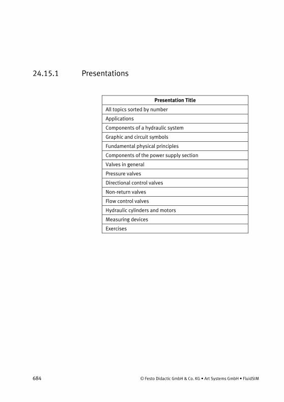
684 © Festo Didactic GmbH & Co. KG • Art Systems GmbH • FluidSIM
24.15.1 Presentations
Presentation Title
All topics sorted by number
Applications
Components of a hydraulic system
Graphic and circuit symbols
Fundamental physical principles
Components of the power supply section
Valves in general
Pressure valves
Directional control valves
Non-return valves
Flow control valves
Hydraulic cylinders and motors
Measuring devices
Exercises

Index
© Festo Didactic GmbH & Co. KG • Art Systems GmbH • FluidSIM 685
Index
3
3/2-way valve ball seat _____________________________________ 601, 602 disc seat _____________________________________ 602, 603 pneumatically operated ________________________ 603, 604 roller operated ____________________________________ 604
4
4/2-way valve disc seat _________________________________________ 605 roller operated ____________________________________ 605
4/3-way valve turning disc principle_______________________________ 605
5
5/2-way valve longitudinal slide principle __________________________ 606 suspended disc seat _______________________________ 607
5/3-way valve pneumatically operated ____________________________ 607
A
air drying absorption _______________________________________ 592 adsorption _______________________________________ 592 low temperature __________________________________ 591
air lubricator _____________________________________ 592, 593 air motor ____________________________________________ 600 air service unit _______________________________________ 590
C
circuit diagram bistable valve ________________________________ 607, 608 direct control _____________________________________ 609 indirect control ___________________________________ 609 pressure sequence valve ___________________________ 621 quick exhaust valve ________________________________ 617 sequential control _________________________________ 625 shuttle valve _________________________________ 614, 615 signal overlap ________________________________ 626, 627

686 © Festo Didactic GmbH & Co. KG • Art Systems GmbH • FluidSIM
time delay valve___________________________________ 623 two pressure valve ____________________________ 612, 613
component animation animation component ______________________________________ 572 description didactics component description ____________________________ 565 sectional view component usage in circuit didactics
sectional view __________________________________ 567 compressed air filter filter ______________________________ 591 compressed air supply
axial flow compressor axial flow compressor ____________ 594 delivery _________________________________________ 593 distribution ______________________________________ 594 piston compressor piston compressor _________________ 594
cylinder control cylinder double acting ____________________________________ 597 single acting _____________________________________ 596 double acting _________________________________ 597, 598 mounting arrangements ____________________________ 598 seals ____________________________________________ 598 single acting _____________________________________ 596 tandem double acting ______________________________ 599
D
Delay Switches ___________________________________ 477, 492 diagram symbol
designation of connections __________________________ 600 directional valve __________________________________ 600 flow control valve _________________________________ 618 linear actuator ____________________________________ 595 method of actuation _______________________________ 601 non-return valve diagram symbol check valve ______________________________________ 611 numbering system _________________________________ 589 pressure control valve ______________________________ 620 rotary actuator ____________________________________ 595 supply component _________________________________ 590
Dialog window diagram properties ________________________________ 339 drawing areas ____________________________________ 342 Functional diagram ________________________________ 338 line options ______________________________________ 348

© Festo Didactic GmbH & Co. KG • Art Systems GmbH • FluidSIM 687
signal logic _______________________________________ 349 signaling elements ________________________________ 345 text options ______________________________________ 340
didactics actuators ________________________________________ 595 applications ______________________________________ 630 basic pneumatics _________________________________ 588 cylinder didactics motor __________________________________________ 669 directional control valves ___________________________ 600 educational film educational film overview ____________________________________ 627, 683 exercises ________________________________________ 673 flow control valves ________________________________ 618 flow valves _______________________________________ 666 gauge ___________________________________________ 672 hydraulic plant ____________________________________ 631 physical fundamentals _____________________________ 637 power unit _______________________________________ 640 presentation presentation play ____________________________________________ 579 presentations overview ________________________________________ 683 presentations presentation overview ________________________________________ 628 pressure control valves _____________________________ 620 pressure valves ___________________________________ 646 sequential circuit didactics signal overlap circuit ______________________________ 625 shutoff valves ________________________________ 611, 662 supply elements __________________________________ 590 symbols _________________________________________ 633 time delay valve___________________________________ 622 tutorial tutorial ___________________________________ 573 valves ___________________________________________ 644 way valves _______________________________________ 653

688 © Festo Didactic GmbH & Co. KG • Art Systems GmbH • FluidSIM
Digital Basic Functions _________________________________ 548 Digital Components ___________________________________ 546 Digital Special Functions _______________________________ 550 Digitale Constants ____________________________________ 546 DIN standard ________________________________________ 565 distance-step diagram _________________________________ 625 Druckschalter ________________________________________ 482
E
electrical components american standard ________________________________ 491 ladder diagram style _______________________________ 491
Electrical Components _________________________________ 468 electronic components _________________________________ 497 exercise
bending machine __________________________________ 674 clamping device ___________________________________ 678 drilling machine ___________________________________ 682 drying oven ______________________________________ 678 embossing press __________________________________ 676 feed control ______________________________________ 680 grinding machine __________________________________ 673 hydraulic crane ___________________________________ 679 ladle ____________________________________________ 677 planing machine __________________________________ 681 roller conveyor ____________________________________ 675
F
function illustration general sectional view ______________________________ 575
G
GRAFCET Elements ____________________________________ 556
L
ladder diagram _______________________________________ 491 Limit Switches ___________________________________ 479, 493
M
measuring devices ____________________________________ 408 measuring instruments ________________________________ 463 menu
context sensitive context sensitive ____________________ 564

© Festo Didactic GmbH & Co. KG • Art Systems GmbH • FluidSIM 689
Miscellaneous _______________________________________ 559
N
non return valve ______________________________________ 612 Numbering __________________________________________ 588
O
one-way flow control valve _________________________ 618, 619
P
Pneumatic Components ________________________________ 410 presentation
creation _________________________________________ 582 edit _____________________________________________ 582
pressure absolute pressure atmospheric _____________________________________ 595
pressure control valve _________________________________ 593 pressure switches ____________________________________ 393 Pressure Switches ____________________________________ 495 Proximity Switches ____________________________________ 484
Q
quick exhaust valve _______________________________ 616, 617
S
semi-rotary actuator ___________________________________ 599 sequence valve _______________________________________ 620 Service Components __________________________________ 352 shuttle valve _________________________________________ 614 signal flow __________________________________________ 588 signal flow component _________________________________ 588 supply air throttling exhaust air throttling _________________ 619 supply elements ______________________________________ 410 switch
pressure operated _________________________________ 443

690 © Festo Didactic GmbH & Co. KG • Art Systems GmbH • FluidSIM
T
Throttle valve ________________________________________ 619 time delay valve delay valve ________________________ 622, 623 two pressure valve ____________________________________ 612
V
valves configurable _________________________________ 360, 417 directional _______________________________________ 364 directional valves _________________________________ 421 flow control ______________________________________ 393 flow control valves ________________________________ 437 groups __________________________________________ 451 pressure _________________________________________ 381 shutoff __________________________________________ 378 shutoff valves ____________________________________ 437 way valves ___________________________________ 360, 417