fluxnet: a new tool to study the temporal and spatial

2415Bulletin of the American Meteorological Society

FLUXNET: A New Tool to Studythe Temporal and Spatial Variabilityof Ecosystem-Scale Carbon Dioxide,

Water Vapor, and Energy Flux DensitiesDennis Baldocchi,a Eva Falge,b Lianhong Gu,a Richard Olson,c David Hollinger,d Steve Running,e

Peter Anthoni,f Ch. Bernhofer,g Kenneth Davis,h Robert Evans,d Jose Fuentes,i Allen Goldstein,a

Gabriel Katul,j Beverly Law,f Xuhui Lee,k Yadvinder Malhi,l Tilden Meyers,m William Munger,n

Walt Oechel,o K. T. Paw U,p Kim Pilegaard,q H. P. Schmid,r Riccardo Valentini,s

Shashi Verma,t Timo Vesala,u Kell Wilson,m and Steve Wofsyn

aESPM, University of California, Berkeley, Berkeley, California.bPflanzenökologie, Universität Bayreuth, Bayreuth, Germany.cEnvironmental Science Division, Oak Ridge National Laboratory, OakRidge, Tennessee.dUSDA Forest Service, Durham, New Hampshire.eSchool of Forestry, University of Montana, Missoula, Montana.fRichardson Hall, Oregon State University, Corvallis, Oregon.gTechnische Universität Dresden, IHM Meteorologie, Tharandt, Germany.hDepartment of Meteorology, The Pennsylvania State University, Univer-sity Park, Pennsylvania.iDepartment of Environmental Science, University of Virginia,Charlottesville, Virginia.jSchool of the Environment, Duke University, Durham, North Carolina.kSchool of Forestry, Yale University, New Haven, Connecticut.lInstitute of Ecology and Resource Management, University of Edinburgh,Edinburgh, United Kingdom.mNOAA/Atmospheric Turbulence and Diffusion Division, Oak Ridge,Tennessee.

ABSTRACT

FLUXNET is a global network of micrometeorological flux measurement sites that measure the exchanges of car-bon dioxide, water vapor, and energy between the biosphere and atmosphere. At present over 140 sites are operating ona long-term and continuous basis. Vegetation under study includes temperate conifer and broadleaved (deciduous andevergreen) forests, tropical and boreal forests, crops, grasslands, chaparral, wetlands, and tundra. Sites exist on five con-tinents and their latitudinal distribution ranges from 70°N to 30°S.

FLUXNET has several primary functions. First, it provides infrastructure for compiling, archiving, and distributingcarbon, water, and energy flux measurement, and meteorological, plant, and soil data to the science community. (Dataand site information are available online at the FLUXNET Web site, http://www-eosdis.ornl.gov/FLUXNET/.) Second,the project supports calibration and flux intercomparison activities. This activity ensures that data from the regionalnetworks are intercomparable. And third, FLUXNET supports the synthesis, discussion, and communication of ideasand data by supporting project scientists, workshops, and visiting scientists. The overarching goal is to provide infor-mation for validating computations of net primary productivity, evaporation, and energy absorption that are beinggenerated by sensors mounted on the NASA Terra satellite.

Data being compiled by FLUXNET are being used to quantify and compare magnitudes and dynamics of annualecosystem carbon and water balances, to quantify the response of stand-scale carbon dioxide and water vapor fluxdensities to controlling biotic and abiotic factors, and to validate a hierarchy of soil–plant–atmosphere trace gas ex-change models. Findings so far include 1) net CO

2 exchange of temperate broadleaved forests increases by about

5.7 g C m−2 day−1 for each additional day that the growing season is extended; 2) the sensitivity of net ecosystem CO2

exchange to sunlight doubles if the sky is cloudy rather than clear; 3) the spectrum of CO2 flux density exhibits peaks

at timescales of days, weeks, and years, and a spectral gap exists at the month timescale; 4) the optimal temperatureof net CO

2 exchange varies with mean summer temperature; and 5) stand age affects carbon dioxide and water vapor

flux densities.

nDepartment of Earth and Planetary Sciences, Harvard University, Cam-bridge, Massachusetts.oDepartment of Biology, San Diego State University, San Diego, California.pLand, Air and Water Resources, University of California, Davis, Davis,California.qPlant Biology and Biogeochemistry Department, Risoe National Labo-ratory, Roskilde, Denmark.rDepartment of Geography, Indiana University, Bloomington, Indiana.sDISAFRI, Universita de Tuscia, Viterbo, Italy.tSchool of Natural Resource Sciences, University of Nebraska at Lincoln,Lincoln, Nebraska.uDepartment of Physics, University of Helsinki, Helsinki, Finland.Corresponding author address: Dennis Baldocchi, Department of Environ-mental Science, Policy and Management, Ecosystems Science Division, 151Hilgard Hall, University of California, Berkeley, Berkeley, CA 94720.E-mail: [email protected] final form 27 February 2001.©2001 American Meteorological Society

2416 Vol. 82, No. 11, November 2001

1. Introduction

Large-scale, multi-investigator projects have beenthe keystone of many scientific and technological ad-vances in the twentieth century. Physicists havelearned much about the structure of an atom’s nucleuswith particle accelerators. Astrophysicists now peerdeep into space with the Hubble Space Telescope andan array of radio telescopes. Molecular biologists aredecoding the structure of our DNA with the HumanGenome project.

Ecosystem scientists need a tool that assesses theflows of carbon, water, and energy to and from theterrestrial biosphere across the spectrum of time- andspace scales over which the biosphere operates (seeRunning et al. 1999; Canadell et al. 2000). Similarly,atmospheric scientists need a tool to quantify surfaceenergy fluxes at the land–atmosphere interface, asthese energy fluxes influence weather and climate(Betts et al. 1996; Pielke et al. 1998). In this paper, wereport on such a tool. It consists of a global array ofmicrometeorological towers that are measuring fluxdensities of carbon dioxide, water vapor, and energybetween vegetation and the atmosphere on a quasi-continuous and long-term (multiyear) basis. The ob-jectives of this paper are to introduce the FLUXNETproject and describe its rationale, goals, measurementmethods, and geographic distribution. We also presenta sampling of new results that are being generatedthrough the project. The intent is to show how infor-mation from this network can aid ecologists, meteo-rologists, hydrologists, and biogeochemists tounderstand temporal and spatial variations that are as-sociated with fluxes of carbon and water between thebiosphere and atmosphere.

2. What is the problem?

Over the past century, the states of the earth’s at-mosphere and biosphere have experienced muchchange. Since the dawn of the industrial revolution, themean global CO

2 concentration has risen from about

280 ppm to over 368 ppm (Keeling and Whorf 1994;Conway et al. 1994). The secular rise in atmosphericcarbon dioxide concentrations is occurring due to im-balances between the rates that anthropogenic andnatural sources emit CO

2 and the rate that biospheric

and oceanic sinks remove CO2 from the atmosphere.

Superimposed on the secular trend of CO2 is a record

of large interannual variability in the annual rate of

growth of atmospheric CO2. Typical values of inter-

annual variability are on the order of 0.5–3.0 ppm yr−1.On a mass basis, these values correspond with a rangebetween 1 and 5 gigatons C yr−1. Potential sources ofyear-to-year changes in atmospheric CO

2 remain a

topic of debate. Studies of atmospheric 13C and O2 dis-

tributions imply that the terrestrial biosphere plays animportant role in this interannual variability (Ciaiset al. 1995; Keeling et al. 1996). Sources of this vari-ability have been attributed to El Niño/La Niña events,which cause regions of droughts or superabundantrainfall (Conway et al. 1994; Keeling et al. 1995), andalterations in the timing and length of the growingseason (Myneni et al. 1997a,b; Randerson et al. 1997).

Rising levels of CO2, and other greenhouse gases,

are of concern to scientists and policy makers becausethey trap infrared radiation that is emitted by theearth’s surface. Potential consequences of elevatedCO

2 concentrations include a warming of the earth’s

surface (Hansen et al. 1998), melting of polar icecapsand a rising sea level, and an alteration of plant andecosystem physiological functioning and plant com-position (Amthor 1995; Norby et al. 1999).

With regard to plants and ecosystems, short-termexperiments with elevated CO

2 show increased rates

of photosynthesis and plant growth and lowered sto-matal conductance (Drake et al. 1996). The long-termsustainability of enhanced rates of growth by plants,however, depends on nutrient and water availability,temperature, and light competition (Ceulemans andMousseau 1994; Norby et al. 1999). Warmer tempera-tures, associated with elevated CO

2, promote increased

rates of respiration when soil moisture is ample. Butif climate warming is associated with drying, there canbe reduced assimilation and lower rates of soil/rootrespiration in temperate ecosystems. In the tundra andboreal forest, warming and drying can lower watertables, exposing organic peat to air and increasing itsrate of respiration (Goulden et al. 1998; Lindroth et al.1998; Oechel et al. 2000).

How evaporation is impacted by elevated CO2 de-

pends on the scale of study and concurrent changes inleaf area index, canopy surface conductance, and thedepth of the planetary boundary layer. Theory indi-cates that complex feedbacks among stomatal conduc-tance, leaf temperature, and the air’s vapor pressuredeficit cause responses at the leaf scale to differ fromthat of the canopy scale. For instance, a potential re-duction of leaf transpiration, by stomatal closure, iscompensated for in part by the entrainment of dry airfrom above the planetary boundary layer and elevated


leaf temperatures and humidities (Jacobs and deBruin1992). Hence, canopy evaporation may not be reducedto the same degree as leaf transpiration in an elevatedCO

2 world.

In the meantime, the composition of the land sur-face has changed dramatically to meet the needs of thegrowing human population. Many agricultural landshave been transformed into suburban and urban land-scapes, wetlands have been drained, and many tropi-cal forests have been logged, burnt, and converted topasture. In contrast, abandoned farmland in the north-east United States and Europe is returning to forestas those societies become more urban. Changes in landuse alter the earth’s radiation balance by changing itsalbedo, Bowen ratio (the ratio between the flux den-sities of sensible and latent heat exchange), leaf areaindex, and physiological capacity to assimilate carbonand evaporate water (Betts et al. 1996; Pielke et al.1998). Changing a landscape from forest to agricul-tural crops, for instance, increases the surface’s albedoand decreases the Bowen ratio (Betts et al. 1996);forests have a lower physiological capacity to assimi-late carbon and a lower ability to transpire water, ascompared to crops (Kelliher et al. 1995; Baldocchi andMeyers 1998). A change in the age structure of for-ests due to direct (deforestation) or indirect (climate-induced fires) disturbance alters its ability to acquirecarbon and transpire water (Amiro et al. 1999; Schulzeet al. 1999).

The issues identified above all require informationon fluxes of carbon, water, and energy at the earth’ssurface and how these fluxes interact with the physi-cal climate and physiological functioning of plants andecosystems. In the next section we identify numerousways to obtain this information and illustrate how anetwork of long flux measurement sites can provideparticularly useful information to study these complexproblems.

3. How to study biosphere CO2exchange?

Study of the earth’s biogeochemistry and hydrol-ogy involves quantifying the flows of matter in andout of the atmosphere. Numerous techniques exist forstudying biosphere–atmosphere CO

2 exchange, each

with distinct advantages and disadvantages. At thecontinental and global scales, scientists assess carbondioxide sources and sinks using atmospheric inversionmodels that ingest information on fields of CO

2, 13C,

and O2 concentration and wind (Tans et al. 1990; Ciais

et al. 1995; Denning et al. 1996; Fan et al. 1998). Thisapproach is subject to errors due to the sparseness ofthe trace gas measurement network, their biased place-ment in the marine boundary layer, and the accuracyof the atmospheric transport models (Tans et al. 1990;Denning et al. 1996; Fan et al. 1998).

Instruments mounted on satellite platforms viewthe earth in total. Consequently, satellite-based instru-ments offer the potential to evaluate surface carbonfluxes on the basis of algorithms that can be driven byreflected and emitted radiation measurements(Running et al. 1999; Cramer et al. 1999). This ap-proach, however, is inferential, so it is dependent onthe accuracy of the model algorithms, the frequencyof satellite images, and the spectral information con-tained in the images.

At the landscape to regional scale we can use in-struments mounted on aircraft (Crawford et al. 1996;Desjardins et al. 1984, 1997) or boundary layer bud-get methods (Denmead et al. 1996; Levy et al. 1999;Yi et al. 2000) to assess carbon and water fluxes.Aircraft-based eddy covariance flux density measure-ments give good information on spatial patterns ofcarbon and water fluxes across transects to tens tohundreds of kilometers. However, they do not provideinformation that is continuous in time, nor do theyprovide insights on the physiological mechanisms thatgovern carbon and water fluxes. Boundary layer bud-get methods can be implemented using tall towers,tethered balloons, or small aircraft. This method pro-vides information on spatially integrated fluxes of tensto hundreds of square kilometers, but it can be appliedonly during ideal meteorological conditions (Denmeadet al. 1996). Routine application of this method is ham-pered by a lack of data on entrainment and horizontaladvection.

One measure of carbon flux “ground truth” can beprovided by biomass surveys (Kauppi et al. 1992;Gower et al. 1999). However, biomass surveys pro-vide information on multiyear to decadal timescales,so they do not provide information on shorter-termphysiological forcings and mechanisms. Furthermore,forest inventory studies are labor intensive and areinferential estimates of net carbon exchange. Suchstudies rarely measure growth of small trees and below-ground allocation of carbon. Instead biomass surveyscommonly assume that a certain portion of carbon isallocated below ground (Gower et al. 1999). Soil car-bon surveys can be conducted too but, like biomasssurveys, they require long intervals to resolve de-

2418 Vol. 82, No. 11, November 2001

tectable differences in net carbon uptake or loss(Amundson et al. 1998).

The eddy covariance method, a micrometeorologi-cal technique, provides a direct measure of net carbonand water fluxes between vegetated canopies and theatmosphere (Baldocchi et al. 1988; Foken and Wichura1996; Aubinet et al. 2000). With current technology,the eddy covariance method is able to measure massand energy fluxes over short and long timescales (hour,days, seasons, and years) with minimal disturbance tothe underlying vegetation. Another attribute of theeddy covariance method is its ability to sample a rela-tively large area of land. Typical footprints have lon-gitudinal length scales of 100–2000 m (Schmid 1994).If deployed as a coordinated network of measurementssites, the eddy covariance method has the potential ofquantifying how whole ecosystems respond to a spec-trum of climate regimes, thereby expanding the spa-tial scope of this method.

The eddy covariance method is not without weak-nesses. Its application is generally restricted to peri-ods when atmospheric conditions are steady and tolocations with relatively flat terrain and vegetation thatextends horizontally about 100 times the samplingheight. Consequently, the method is not suitable formeasuring fluxes in rough mountainous terrain or neardistinct landscape transitions such as lakes.

Nevertheless, the strengths of the eddy covariancemethod far outweigh its weaknesses, as it can provideinformation that can aid in inferential carbon fluxesbeing determined by the global inversion model com-munity, remote sensing scientists, and forest ecolo-gists. For example, data from an eddy covariancemeasurement site have the potential to complementthe global flask sampling network in a very direct way.Historically, the global flask sampling network hasbeen concentrated at marine locations (Tans et al.1990). Recent studies using tall towers show that thereare times during the day, when either local surfacefluxes are small or convective mixing is vigorous, thatCO

2 concentrations measured in the atmospheric sur-

face layers are very close to the mean boundary layerconcentration (Bakwin et al. 1998; Potosnak et al.1999). High-precision CO

2 concentration measure-

ments and surface carbon flux measurements, made ateddy covariance measurement sites, have the poten-tial to expand the density of the existing flask network.Data from a network of eddy covariance measurementsites can also be used to improve and validate the al-gorithms being used by remote sensing scientists andecosystem modelers. And finally, such data can aid

forest ecologists in their interpretation of forest bio-mass inventories, by providing information on fluxesfrom carbon pools and how these fluxes vary on a sea-sonal and interannual basis.

4. History: What has been done?

Micrometeorologists have been measuring CO2

and water vapor exchange between vegetation and theatmosphere since the late 1950s and early 1960s. Yet,only recently have we had the technology availablethat enables us to make continuous flux measurementsat numerous sites.

The earliest reported micrometeorological mea-surements of CO

2 exchange were conducted by Inoue

(1958), Lemon (1960), Monteith and Sziecz (1960),and Denmead (1969). These studies employed theflux-gradient method over agricultural crops duringthe growing season. By the late 1960s and early 1970s,a few scientists started applying the flux-gradientmethod over natural landscapes. Several flux-gradientstudies of CO

2 exchange were conducted over forests

(Denmead 1969; Baumgartner 1969; Jarvis et al. 1976),and one team ventured to assess the annual carbonbalance of a salt marsh (Houghton and Woodwell 1980).

As more data were collected it became evident thatthe flux-gradient method was suffering from majordeficiencies, when applied over tall forests. One flawarose from large-scale transport in the roughnesssublayer, which caused local eddy exchange coeffi-cients to be enhanced relative to estimations based onMonin–Obukhov scaling theory (Rapauch and Legg1984; Kaimal and Finnigan 1994). The flux-gradientmethod also failed to provide reliable means of evalu-ating eddy exchange coefficients at night.

Routine application of the eddy covariance methodwas delayed until the 1980s, when technological ad-vances in sonic anemometry, infrared spectrometry,and digital computers were made. Initial studieswere conducted over crops (Anderson et al. 1984;Desjardins et al. 1984; Ohtaki 1984), forests (Vermaet al. 1986), and native grasslands (Verma et al. 1989)for short intense periods during the peak of the grow-ing season. By the late 1980s and early 1990s, the fur-ther technological developments, such as larger datastorage capacity and linear and nondrifting instru-ments, enabled scientists to make defensible measure-ments of eddy fluxes for extended periods. Wofsy et al.(1993), at Harvard Forest, and Vermetten et al. (1994),in the Netherlands, were among the first investigators


to measure carbon dioxide and water vapor fluxes con-tinuously over a forest over the course of a year withthe eddy covariance method. Spurred by these twopioneering studies, a handful of other towers were soonestablished and operating by 1993 in North America[Oak Ridge, Tennessee (Greco and Baldocchi 1996);Prince Albert, Saskatchewan, Canada (Black et al. 1996)]and Japan (Yamamoto et al. 1999), and in Europe by1994 (Valentini et al. 1996). This era also heralded thestart of longer, quasi-continuous multi-investigatorexperiments. Noted examples include the BorealEcosystem–Atmosphere Study (Sellers et al. 1997)and the Northern Hemisphere Climate-ProcessesLand–Surface Experiment (Halldin et al. 1999).

The next natural step in the evolutionary develop-ment of this field was to establish a global network ofresearch sites. The concept of a global network of long-term flux measurement sites had a genesis as early as1993, as noted in the science plan of the InternationalGeosphere–Biosphere Program/Biospheric Aspects ofthe Hydrological Cycle (BAHC Core Project Office1993). Formal discussion of the concept among theinternational science community occurred at the 1995La Thuile workshop (Baldocchi et al. 1996). At thismeeting, the flux measurement community discussedthe possibilities, problems, and pitfalls associated withmaking long-term flux measurements (e.g., Gouldenet al. 1996a,b; Moncreiff et al. 1996). After the La Thuilemeeting there was acceleration in the establishment offlux tower sites and regional flux measurement net-works. The Euroflux project started in 1996 (Aubinetet al. 2000; Valentini et al. 2000). The AmeriFluxproject was conceived in 1997, subsuming the several

ongoing tower studies and initiating many new stud-ies. With the success of the European and Americanregional networks and anticipation of the Earth Ob-servation Satellite (EOS/Terra), the National Aero-nautics and Space Administration (NASA) decided,in 1998, to fund the global-scale FLUXNET project,as a means of validating EOS products.

5. What is being done?

The FLUXNET project serves as a mechanism foruniting the activities of several regional and continen-tal networks into an integrated global network. Atpresent over 140 flux tower sites are registered on theFLUXNET data archive. Research sites are operatingacross the globe (Fig. 1) in North, Central, and SouthAmerica; Europe; Scandinavia; Siberia; Asia; and Africa.The regional networks include AmeriFlux [which in-cludes Large-scale Biosphere–Atmosphere Experi-ment (LBA) sites in Brazil], CarboEuroflux (whichhas subsumed Euroflux and Medeflu), AsiaFlux, andOzFlux (Australia, New Zealand). There are also dis-parate sites in Botswana and South Africa.

The global nature of FLUXNET extends the di-versity of biomes, climate regions, and methods that areassociated with the regional networks. For example,sites in the original Euroflux network consisted ofconifer and deciduous forests and Mediterraneanshrubland. The European networks also used a stan-dard methodology, based on closed-path infrared spec-trometers (Aubinet et al. 2000; Valentini et al. 2000).By contrast, the American network, AmeriFlux, has

FIG. 1. Global map of FLUXNET field sites.

2420 Vol. 82, No. 11, November 2001

more diversity in terms of the number of biomes andclimates studied and methods used. The American re-gional network includes sites in temperate conifer anddeciduous forests, tundra, cropland, grassland, chap-arral, boreal forests, and tropical forests. Regardingmethodology, open- and closed-path infrared spec-trometers are used to measure CO

2 and water vapor

fluctuations. Another unique dimension of AmeriFluxis its inclusion of a tall (400 m) tower (Bakwin et al.1998; Yi et al. 2000) for study of CO

2 flux and con-

centration profiles and boundary layer evolution.The placement of field sites in FLUXNET has

been ad hoc, due to limited funding and investigatorcapabilities, rather than following a predeterminedgeostatistical design. So with the current network con-figuration, we are not capable of measuring fluxesfrom every patch on earth, nor do we intend to. Onthe other hand, this coordinated network of sites is ableto deduce certain information on spatial patterns offluxes by placing research sites across a spectrum ofclimate and plant functional regions (Running et al.1999). Spatially integrated fluxes of carbon and wa-ter can only be constructed by combining eddy fluxmeasurements with ecosystem and biophysical mod-els and satellite measurements to perform the spatialintegration (Running et al. 1999).

The scientific goals of FLUXNET are to

1) quantify the spatial differences in carbon dioxideand water vapor exchange rates that may be expe-rienced within and across natural ecosystems andclimatic gradients;

2) quantify temporal dynamics and variability (sea-sonal, interannual) of carbon, water, and energyflux densities—such data allow us to examine theinfluences of phenology, droughts, heat spells,El Niño, length of growing season, and presenceor absence of snow on canopy-scale fluxes; and

3) quantify the variations of carbon dioxide and watervapor fluxes due to changes in insolation, tempera-ture, soil moisture, photosynthetic capacity, nutrition,canopy structure, and ecosystem functional type.

FLUXNET has two operational components, aproject office and a data archive office. The project of-fice houses the principal investigator and a postdoctoralscientist. Specific duties of the FLUXNET office include

1) communicating with participants to ensure thetimely submission of data and documentation tothe data archive,

2) constructing and analyzing integrated datasets forsynthesis of field data and for the development andtesting of soil–atmosphere–vegetation–transfermodels,

3) organizing workshops for data synthesis and modeltesting activities,

4) preparing peer-reviewed research papers and re-ports on FLUXNET activities and analyses,

5) funding the execution and analysis of site inter-comparison studies, and

6) providing scientific guidance to the FLUXNETData and Information System (DIS).

The data archive office is responsible for

1) compiling and documenting data in consistentformats,

2) developing data guidelines and coordinating devel-opment of the FLUXNET DIS,

3) scrutinizing datasets with standard quality controland assurance procedures,

4) maintaining the FLUXNET Web page for com-munications and data exchange (http://www-eosdis.ornl.gov/FLUXNET/), and

5) transferring FLUXNET data and metadata to along-term archive, currently designated as the OakRidge National Laboratory Distributed ActiveArchive Center.

Back up of data and long-term accessibility of the data,provided by FLUXNET DIS, ensures the protectionand extended use of the data by project scientists, aswell as students and citizens, well into the future.

FLUXNET does not fund tower sites directly, butdepends upon institutional support associated with thefunding of the AmeriFlux, CarboEuroflux, AsiaFlux,and OzFlux networks (see acknowledgments).

MethodologyThe eddy covariance method is used to assess trace

gas fluxes between the biosphere and atmosphere ateach site within the FLUXNET community (Aubinetet al. 2000; Valentini et al. 2000). Vertical flux densi-ties of CO

2 (F

c) and latent (λE) and sensible heat (H)

between vegetation and the atmosphere are propor-tional to the mean covariance between vertical veloc-ity (w′) and the respective scalar (c′) fluctuations (e.g.,CO

2, water vapor, and temperature). Positive flux den-

sities represent mass and energy transfer into the at-mosphere and away from the surface, and negativevalues denote the reverse; ecologists use an opposite


sign convention where the uptake of carbon by thebiosphere is positive. Turbulent fluctuations werecomputed as the difference between instantaneous andmean scalar quantities.

Our community is interested in assessing the netuptake of carbon dioxide by the biosphere, not the fluxacross some arbitrary horizontal plane. When the ther-mal stratification of the atmosphere is stable or turbu-lent mixing is weak, material diffusing from leaves andthe soil may not reach the reference height z

r in a time

that is short compared to the averaging time T, therebyviolating the assumption of steady-state conditions anda constant flux layer. Under such conditions the stor-age term becomes nonzero, so it must be added to theeddy covariance measurement to represent the balanceof material flowing into and out of the soil and veg-etation (Wofsy et al. 1993; Moncrieff et al. 1996). Withrespect to CO

2, the storage term is small over short

crops and is an important quantity over taller forests.The storage term value is greatest around sunrise andsunset, when there is a transition between respirationand photosynthesis and between the stable nocturnalboundary layer and daytime convective turbulence(Aubinet et al. 2000; Yi et al. 2000). Summed over24 h, the storage term is nil (Baldocchi et al. 2000).

Horizontal advection is possible when vegetationis patchy or is on level terrain (Lee 1998; Finnigan1999). At present, routine corrections for advectionmay require a three-dimensional array of towers(Finnigan 1999), rather than the application of a ver-tical velocity advection correction (see Lee 1998;Baldocchi et al. 2000).

6. Instrumentation, data acquisition,and processing

Typical instrumentation at FLUXNET field sitesincludes a three-dimensional sonic anemometer, tomeasure wind velocities and virtual temperature, anda fast responding sensor to measure CO

2 and water

vapor. Scalar concentration fluctuations are measuredwith open- and closed-path infrared gas analyzers.Standardized data processing routines are used to com-pute flux covariances (Foken and Wichura 1996;Moncrieff et al. 1996; Aubinet et al. 2000).

Application of the eddy covariance methods in-volves issues relating to site selection, instrumentplacement, sampling duration and frequency, calibra-tion and postprocessing (Moore 1986; Baldocchi et al.1988; Foken and Wichura 1996; Moncrieff et al. 1996;

Aubinet et al. 2000). Ideally the field site should beflat, with an extensive fetch of uniform vegetation. Inpractice many of the FLUXNET sites are on undulat-ing or gently sloping terrain, as this is where nativevegetation exists. Sites on extreme terrain, which mayforce flow separation and advection, are excluded. Thedegree of uniformity of the underlying vegetation var-ies across the network, too. Some sites consist ofmonospecific vegetation, others contain a mixture ofspecies and a third grouping possesses different plantfunctional types in different wind quadrants. All siteshave sufficient fetch to generate an internal boundarylayer where fluxes are constant with height (Kaimaland Finnigan 1994).

Agricultural scientists mount their sensors on smallpoles, while forest scientists use either walk-up scaf-folding or low-profile radio towers. The height of thesensors depends on the height of the vegetation, theextent of fetch, the range of wind velocity, and the fre-quency response of the instruments. To minimizetower interference on scaffold towers, investigatorsplace their instruments booms so that they point sev-eral meters upwind or at the top of the tower. Spatialseparation between anemometry and gas analyzersdepend on whether one uses a closed- or open-path gassensor. With the closed-path systems, the intake isoften near or within the volume of the sonic anemom-eters. A delay occurs as air flows through the tubingto the sensor, which is compensated for with softwareduring postprocessing. Some investigators place theirgas transducer on the tower in a constant environmentbox to minimize the lag time from the sample port andthe sensor. Others draw air down long tubes to instru-ments housed in an air-conditioned hut below thetower. In either circumstance, flow rates are high(6 L min−1) to ensure turbulent flow and minimize thediffusive smearing of eddies (Aubinet et al. 2000).Open-path gas sensors are typically placed within0.5 m of a sonic anemometer, a distance that mini-mizes flow distortion and lag effects (Baldocchi et al.2000; Meyers 2001).

Sampling rates between 10 and 20 Hz ensure com-plete sampling of the high-frequency portion of theflux cospectrum (Anderson et al. 1984). The samplingduration must be long enough to capture low-frequency contributions to flux covariances, but nottoo long to be affected by diurnal changes in tempera-ture, humidity, and CO

2. Adequate sampling duration

and averaging period vary between 30 and 60 min(Aubinet et al. 2000). Coordinate rotation calculationsof the orthogonal wind vectors (w,u,v) are performed

2422 Vol. 82, No. 11, November 2001

to correct for instrument misalignment and nonlevelterrain. The vertical velocity, w, is rotated to zero,allowing flux covariances to be computed orthogonalto the mean streamlines.

Calibration frequencies of gas instruments varyfrom team to team. With closed-path sensors, investi-gators are able to calibrate frequently and automati-cally, such as hourly or once a day. Teams withopen-path sensors calibrate less frequently, for ex-ample, every few weeks. However, a body of accumu-lating data indicates that calibrating coefficients ofcontemporary instruments remain steady within thatduration (±5%; Meyers 2001). Scientists using open-path sensors also compare their instrument responsesto an independent measure of CO

2 concentration and

humidity. Members of this network do not use a uni-form standard for calibration CO

2, yet. But many of us

use CO2 gas standards that are traceable to the standards

at the Climate Monitoring and Diagnostics Laboratoryof the National Oceanic and Atmospheric Administra-tion, the standards of the global flask network.

To ensure network intercomparability, the AmeriFluxproject circulates a set of reference sensors to mem-bers in the network, and the FLUXNET project spon-sors the circulation of this set of instruments to sitesin Europe, Asia, and Australia. Figure 2 shows a typi-cal comparison between the roving set of referenceinstrumentation and data from one research group.Carbon dioxide flux densities measured by the twosystems agree within 5% of one another on an hour-by-hour basis. A similar level of agreement has been

found by comparing open- and closed-path CO2 sen-

sors. Side-by-side comparisons between open- andclosed-path water vapor sensors, on the other hand, arenot as good. The absorption and desportion of watervapor on tubing walls can cause water uptake to beunderestimated by 20%.

a. Gap fillingMost clients of eddy flux data, for example mod-

elers, require uninterrupted time series. It is the intentof the micrometeorological community to collect eddycovariance data 24 hours a day and 365 days a year.However, missing data in the archived records is acommon feature. Gaps in the data record are attributedto system or sensor breakdown, periods when instru-ments are off-scale, when the wind is blowing througha tower, when spikes occur in the raw data, when thevertical angle of attack by the wind vector is too se-vere, and when data are missing because of calibrationand maintenance. Other sources of missing data arisefrom farming operations and other management activi-ties (e.g., prescribed burn of grasslands). Rejection cri-teria applied to the data vary among the flux towergroups. Data might be rejected, when stationarity testsor integral turbulence characteristics fail (Kaimal andFinnigan 1994; Foken and Wichura 1996), when pre-cipitation limits the performance of open-path sensors,during sensor calibration, or when spikes occur in in-strument readings. Other criteria used to reject datainclude applications of biological or physical con-straints (lack of energy balance closure; Aubinet et al.2000) and a meandering flux-footprint source area(e.g., Schmid 1994). If the wind is coming from anonpreferred direction as may occur over mixed stands,a certain portion of the data will need to be screened.In addition, rejection probability for some sites is higherduring nighttime because of calm wind conditions.

The average data coverage during a year is between65% and 75% due to system failures or data rejection(Falge et al. 2001). Tests show that this observed levelof data acceptance provides a statistically robust andoversampled estimate of the ensemble mean. So thefilling of missing data does not provide a significantsource of bias error.

b. Accuracy assessmentErrors associated with the application of the eddy

covariance method can be random or biased (Moncrieffet al. 1996). Random errors arise from sensor noise andthe random nature of atmospheric turbulence. Fullysystematic bias errors arise from errors due to sensor

FIG. 2. A comparison of CO2 flux densities between the

FLUXNET reference set of instruments and instruments at theItalian CarboEuroflux site. Here b(0) is the zero intercept andb(1) is the slope of the regressive curve, and r2 is the coefficientof determination.


drift, limited spectral response of instruments, limitedsampling duration and frequency, and calibration er-rors. Selectively systematic bias errors arise from mis-application of the eddy covariance method, as whenadvection or storage occurs. Formal discussions on er-rors associated with long-term flux measurementswere reported in previous papers by our colleagues(e.g., Goulden et al. 1996a; Moncrieff et al. 1996;Aubinet et al. 2000). For clarification, we provide asummary of their findings. Moncrieff et al. (1996)demonstrate how random sampling errors diminishgreatly as the number of samples increase. The over-all random error using a dataset of 44 days is about0.4 µmol m−2 s−1. This figure of merit is close to the“flux detection” level that many of us see with our fieldmeasurements. Accumulated over a year, this randomerror is ±53 g C m−2 yr−1, a value that agrees with aformal error analysis by Goulden et al. (1996a,b).

Fully systematic bias errors associated with imper-fect sensor response, sensor orientation, and samplingfrequency and duration are typically compensated byapplying spectral transfer functions to the flux cova-riance calculations (Moore 1986; Massman 2000).Depending on instrument configuration, wind speed,and thermal stratification, corrections can range froma few to 50 percent.

Selectively systematic bias errors are more diffi-cult to assess. A cohort of carbon flux researchers sus-pect that they may be underevaluating the nighttimemeasure of CO

2 fluxes, despite attempts to measure

the storage term (Black et al. 1996; Goulden et al.1996a; Baldocchi et al. 2000; Aubinet et al. 2000).Potential explanations include insufficient turbulentmixing, incorrect measurement of the storage term ofCO

2 in the air space and soil, and the drainage of CO

2

out of the canopy volume at night. At present, severalteams of investigators are applying an empirical cor-rection to compensate for the underestimation of night-time carbon flux measurements. This correction is basedon CO

2 flux density measurements obtained during

windy periods or by replacing data with a temperature-dependent respiration function (Black et al. 1996;Goulden et al. 1996a,b; Lindroth et al. 1998). Mostresearchers presume that data from windy periods rep-resent conditions when the storage and drainage ofCO

2 is minimal (Aubinet et al. 2000).

When using FLUXNET data, the user should rec-ognize that some sites are more suitable for construct-ing annual sums than others. Yet good science can beproduced from the nonideal sites, too. They can pro-vide information on physiological functioning, tem-

poral dynamics, and response to the environment dur-ing the day. We also note that the factors that causelarge bias errors associated with nocturnal CO

2 fluxes

may not cause significant errors to water vapor fluxes,since evaporative fluxes are near zero during the night.Consequently, studies comparing integrated annualmeasurements of evaporation with lysimeters andwatersheds show good agreement (Barr et al. 2000;Wilson et al. 2000). On the other hand, tests of sur-face energy balance closure suggest that turbulentfluxes at some sites are systematically 10% to 30% toosmall to close the energy budget, raising the possibil-ity that CO

2 fluxes are similarly underestimated

(Aubinet et al. 2000). The solution to this problemremains unresolved at the time of this writing.

7. Recent findings

As we write this report, 69 site-years of carbondioxide and water vapor flux data have been publishedin the literature. Table 1 presents a survey of the an-nual sums of net carbon dioxide exchange. Most sitesare net sinks of CO

2 on an annual basis. Magnitudes

of net carbon uptake by whole ecosystems range fromnear zero to up to over 700 g C m−2 yr−1. Largest val-ues of carbon uptake are associated with temperate for-ests (conifer and deciduous) growing near the southernedge of that climate range. The substantial rate of netcarbon uptake by tropical and temperate forests sites,under study, is an indicator that these sites have expe-rienced substantial amounts of disturbances in the rela-tively near past (50–100 yr) and have not reachedlong-term steady state.

On close inspection of Table 1, we note that sev-eral sites are sources of CO

2. Sites losing carbon di-

oxide include boreal forests and tundra, which areexperiencing disturbance of long-term carbon storagepools (Goulden et al. 1998; Lindroth et al. 1998;Oechel et al. 2000), and grasslands, which were burnt(Suyker and Verma 2000) or were suffering fromdrought (Meyers 2001). The maximum carbon lost bythese sites on an annual basis does not exceed100 g C m−2.

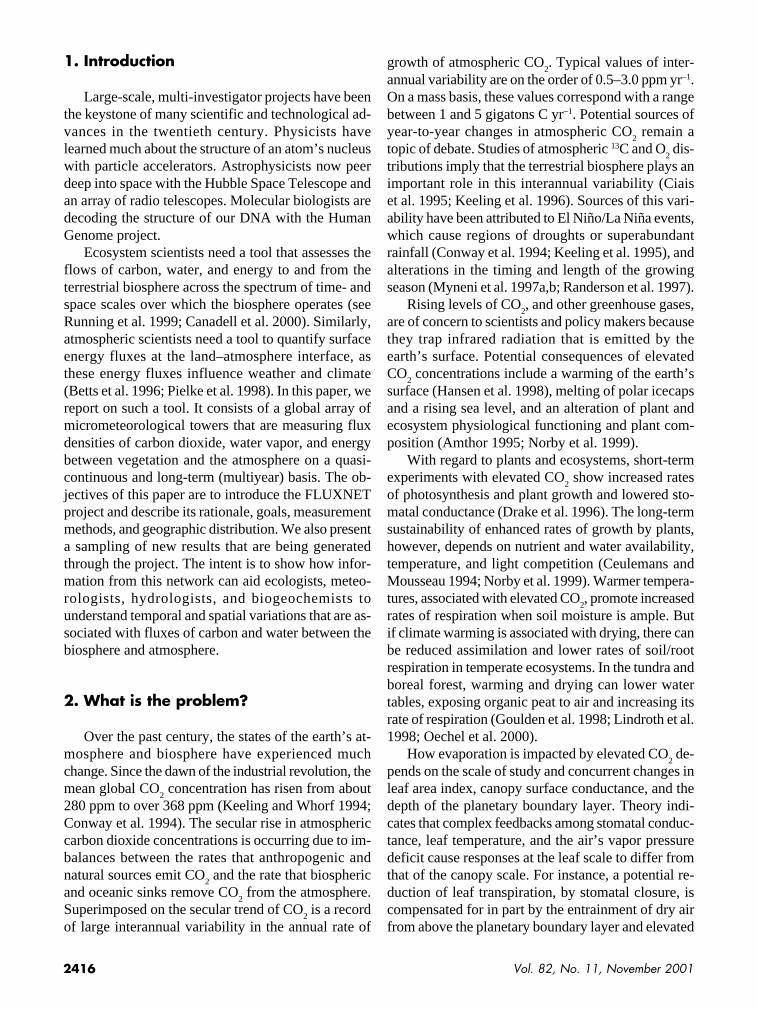
With the plethora of long-term carbon flux dataavailable, we can quantify seasonal patterns of carbonfluxes across a variety of climates, biomes, and plantfunctional groups. Figure 3 shows the annual patternof weekly CO

2 exchange for several temperate broad-

leaved deciduous forests. Broadleaved forests losecarbon during the winter, when they are leafless and

2424 Vol. 82, No. 11, November 2001

a. Temperate broadleaved deciduous forests

Italy Beech, Fagus −470 1994 R. Valentini Valentini et al. (1996)

France Beech, Fagus −218 1996 A. Granier Granier et al. (2000)−257 1997

Denmark Beech, Fagus −169 1997 N. O. Jensen Pilegaard et al. (2001)−124 1998

Iceland Poplar −100 1997 H. Thoreirsson Valentini et al. (2000)

Saskatchwan, Aspen −160 1994 T. A. Black Black et al. (1996)Canada −144 1994

−80 1996−116 1997−290 1998

Oak Ridge, TN Acer, Quercus −525 1994 D. Baldocchi Greco and−610 1995 Baldocchi (1996);

Maple, oak −597 1996 Wilson and−652 1997 Baldocchi (2000)−656 1998−739 1999

Petersham, MA Acer, Quercus −280 1991 S. Wofsy Wofsy et al. (1993)−220 1992

Maple, oak −140 1993 Goulden et al.−210 1994 (1996a,b)−270 1995

Borden, ON, Canada Maple, Acer −80 1996 X. Lee/J. Fuentes Lee et al. (1999)−270 1997−200 1998

Indiana Deciduous forest −240 1998 H. P. Schmid Schmid et al. (2000)

Takayama, Japan Broadleaf deciduous −120 1994 Yamomoto et al.−70 1995 (1999)

−140 1996−150 1997−140 1998

b. Mixed deciduous and evergreen forests, temperate and Mediterranean

Belgium Conifer and broadleaf −430 1997 M. Aubinet Valentini et al. (2000)

Belgium Conifer and broadleaf −157 1997 R. Ceulemans Valentini et al. (2000)

c. Tropical forests

Amazon Tropical forest −102 1995 J. Grace Malhi et al. (1998)

d. Needleleaf, evergreen, conifer forests

Sweden Pinus sylvestris 90 1995 A. Lindroth Lindroth et al. (1998)−5 199680 1997

Picea abies −190 1997

Italy Picea abies −450 1998 R. Valentini Valentini et al. (2000)

TABLE 1. List of published yearlong studies of net biosphere–atmosphere CO2 exchange, N

e. Negative signs represent a loss of

carbon from the atmosphere and a net gain by the ecosystem.

Ne

Observation PrincipalSite Vegetation (g C m−2 yr−1) year investigator Citation


d. Needleleaf, evergreen, conifer forests

France Pinus pinaster −430 1997 P. Berbigier Berbigier et al. (2001)

Germany Picea abies −77 1997 Valentini et al. (2000)

Germany Picea abies −330 1996 Ch. Bernhofer Valentini et al. (2000)−480 1997

−45 1998

Germany Conifer −310 1996 A. Ibrom Valentini et al. (2000)−490 1997

Germany Picea abies −77 1997 E.-D. Schulze Valentini et al. (2000)

Netherlands Pinus sylvestris −210 1997 H. Dolman Valentini et al. (2000)

United Kingdom Picea sitchensis −670 1997 J. Moncrieff Valentini et al. (2000)−570 1998 Valentini et al. (2000)

Finland Pinus sylvestris −230 1997 T. Vesala Valentini et al. (2000)−260 1998 Markkanen et al.−190 1999 (2001)

Howland, ME Conifer −210 1996 D. Hollinger Hollinger et al. (1999)

Florida Slash pine −740 1996 H. Gholz Clark et al. (1999)−610 1997

Florida Cypress −84 1996 H. Gholz Clarke et al. (1999)−37 1997

Manitoba, Canada Picea mariana 70 1995 Goulden et al. (1998)20 1996

−10 1997

Metolius, OR Pinus ponderosa −320 1996 B. Law Anthoni et al. (1999)−270 1997

Wind River, WA Pseudotsuga menzieii −167 1998 K. T. Paw U Paw U et al. (2000,to −220 unpublished manuscript)

Prince Albert, Picea mariana −68 1995 P. Jarvis Malhi et al. (1999)SK, Canada

e. Broadleaved evergreen, Mediterranean forests

Italy Quercus ilex −660 1997 R. Valentini Valentini et al.(2000)

f. Grassland

Ponca, OK Tall−grass prairie 0 1997 S. B. Verma Suyker and Verma(2001)

Little Washita, OK Grazed grassland 41 1997 Meyers (2001)

g. Tundra

Alaska Tundra 40 W. Oechel Oechel et al. (2000)

TABLE 1. Continued.

Ne

Observation PrincipalSite Vegetation (g C m−2 yr−1) year investigator Citation

2426 Vol. 82, No. 11, November 2001

dormant, and gain carbon during the summer grow-ing season. What differs most among broadleaved for-est sites is the timing of the transition between gainingand losing carbon. The site in the southeastern UnitedStates (Tennessee) is the first to experience springgrowth and photosynthesis, followed by the site inDenmark and one in the northeast United States (Mas-sachusetts). The Harvard Forest in Massachusetts ison the eastern side of the North American continent.It experiences a later spring than the more northerlyDanish site because the climate of Denmark is mod-erated by the Gulf Stream. During the peak of thegrowing season, these three sites, separated by sev-eral thousand kilometers, experience similar dailysums of carbon uptake (around weeks 23–24). Andthe two North American sites, separated by over1000 km, experience similar weekly sums of net CO

2

exchange from about week 23 to 35. In the autumn,the Danish site is the first to drop leaves and respire,and the most southern site is last. Another feature tobe gathered from this figure is how ideal and nonidealsites affect the measurement of respiration. During thewinter the Tennessee site experiences extremely lowrates of respiration. This site is situated on rolling ter-rain and near several power plants. Cold air drainagecauses CO

2 to drain out from under the flux tower,

and plume impaction causes downward carbon fluxesthat counter the upward respiratory flux.

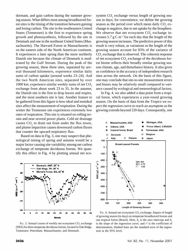
Based on data in Fig. 3, one may suspect that phe-nological timing of spring and autumn would be amajor factor causing site variability among net carbonexchange of temperate deciduous forests. We quan-tify this effect in Fig. 4 by plotting annual net eco-

system CO2 exchange versus length of growing sea-

son in days; for convenience, we define the growingseason as the period over which mean daily CO

2 ex-

change is negative, due to net uptake by the biosphere.We observe that net ecosystem CO

2 exchange in-

creases 5.7 g C m−2 for each day that the length of thegrowing season increases. The predictive power of thisresult is very robust, as variations in the length of thegrowing season account for 83% of the variance ofCO

2 exchange that is observed. The coherent response

of net ecosystem CO2 exchange of the deciduous for-

est biome reflects their broadly similar growing sea-son climate, age, and disturbance history. It also givesus confidence in the accuracy of independent researchsites across the network. On the basis of this figure,one may conclude that site-to-site measurement errorsand biases may be relatively small compared to vari-ance caused by ecological and meteorological factors.

In Fig. 4, we also added a data point from a tropi-cal forest, which experiences a year-round growingseason. On the basis of data from the Tropics we ex-pect the regression curve to reach an asymptote as thegrowing extends beyond 220 days. Consequently, one

FIG. 3. Annual course of weekly net ecosystem CO2 exchange

(NEE) for three temperate deciduous forests, located in Oak Ridge,Tennessee; Petersham, Massachusetts; and Denmark.

FIG. 4. Annual net ecosystem CO2 exchange: Impact of length

of growing season (in days) on temperate broadleaved forests andone tropical forest (Brazil). Here, b

0 is the zero intercept and b

1

is the slope of the regression curve, and r2 is the coefficient ofdetermination. Dashed lines are the standard error of the regres-sion at the 95% level.


should not extrapolate the regression line out to 365days. Nor do we advocate using this plot for estimat-ing year-to-year variability in net ecosystem CO

2 ex-

change at a site. To illustrate this point we show anexample of year-to-year variation of the annual cycleof CO

2 exchange at Harvard Forest (Fig. 5), the site

with the world’s longest measurement record. Otherfactors, such as the presence or absence of snow cover,degree of cloudiness (Goulden et al. 1996b; Lee et al.1999), and drought (Wilson and Baldocchi 2000) im-pose variance on the annual carbon budget, too.

The seasonal trend of CO2 exchange experienced

by conifer forests is affected by latitudinal differences,which shorten or lengthen the growing season, andby continental position, which forces conifer ecosys-tems to experience oceanic, Mediterranean, or conti-nental climates. To illustrate these points we presentdata on seasonal patterns of net CO

2 exchange from

three contrasting conifer forest systems (Fig. 6). TheNorth Carolina site is at a temperate and humid lo-cale in the southeastern United States. There, thecanopy is able to take up carbon all year. The Oregonsite experiences cool, wet winters and dry, warm sum-mers. It assimilates carbon during the late winter,spring, and autumn, but experiences large reductionsin carbon dioxide uptake during the dry summergrowing season (there are instances when it loses car-bon, too). The Finnish site is in the boreal zone. Thetrees are dormant during the cold winter, but the for-est stand loses carbon due to soil and microbial res-piration under the snow pack. In the spring, the onsetof photosynthesis is much delayed compared to themore southerly temperate sites, and its conclusion issooner in the autumn.

With longer datasets, alternative analytical meth-ods can be used to interpret them. Application of Fou-rier transforms to yearlong and multiyear fluxmeasurement records provides a means of quantify-ing the timescales of flux variance (Baldocchi et al.2001). The dominant time periods over which carbondioxide fluxes vary can be days, weeks, seasons, andyears. Figure 7 shows the power spectra of CO

2 fluxes

FIG. 5. Year-to-year variation in the annual cycle of monthlyCO

2 exchange at Harvard Forest, a broadleaved deciduous forest.

FIG. 6. Seasonal course of net weekly CO2 exchange over con-

trasting conifer forests during 1997.

FIG. 7. Power spectrum of CO2 flux over the course of a year

at sites of contrasting climate, functionality, and structure. Powerspectra for the other sites were derived from time series of 1 yrin duration. The power spectra on the y axis are multiplied bynatural frequency (n) and are normalized by variance.

2428 Vol. 82, No. 11, November 2001

over a variety of field sites on a daily timescale. Thesevariations in CO

2 and water vapor exchange are forced

by daily rhythms in solar radiation, air and soil tem-perature, humidity, CO

2, stomatal aperture, photosyn-

thesis, and respiration. On a weekly timescale,fluctuations in CO

2 and water vapor exchange are in-

duced at midlatitude sites from synoptic weatherchanges that are associated with the passage of highand low pressure systems and fronts. Weather eventscause distinct periods of clear sky, overcast, and partlycloudy conditions, which alter the amount of availablelight to an ecosystem, how light is transmitted througha plant canopy, and the efficiency by which it is usedto assimilate carbon (Gu et al. 1999). The passing ofweather fronts also changes air temperature, humid-ity deficits, and pressure. On seasonal timescales,changes in the sun’s position alter the amount of sun-light received, the air, soil, and surface temperature ofthe ecosystem, and its water balance. Superimposedupon these meteorological factors is a variance causedby phenology and seasonal changes in photosyntheticcapacity (Wilson et al. 2000). The timing and occur-rence of leaf expansion, senescence, leaf fall, fine rootgrowth and turnover, and seasonal changes in photo-synthetic capacity and leaf area index are examples ofphenological factors affecting low-frequency fluctua-tions in canopy CO

2 exchange. Prolonged wet and dry

spells are other factors that exert variance on the spec-tral record.

Canopy-scale quantum yield represents the initialslope of the relation between net ecosystem CO

2 ex-

change and the photosynthetic photon flux density.Canopy-scale quantum yield is of particular interest,as it is a parameter used by many biogeochemical car-

bon cycling models to translate remotely sensed ra-diation measurements to an areawide estimate of car-bon uptake (Ruimy et al. 1995; Cramer et al. 1999).Figure 8 shows that the canopy-scale quantum yielddepends on the sky conditions, as well as temperature.The canopy-scale quantum yield is nearly double un-der cloudy skies, as compared to clear skies.

Combining data from the North American andEuropean networks gives us a wider breadth of infor-mation on how CO

2 flux densities respond to tempera-

ture. The temperate zone of Europe is displacednorthward, as compared to North America, due to thepresence of the Gulf Stream. Summer temperaturesin Europe are on the order of 15°–20°C, while in NorthAmerica summer temperatures are in the range of 20°–30°C. Figure 9 indicates that the temperature at whichpeak gross CO

2 exchange occurs is several degrees

lower for many European sites than for their NorthAmerican counterparts. These data suggest that glo-bal carbon flux models will need to vary CO

2 flux–

temperature response curves for North America andEurope, in support of findings by Niinemets et al.(1999).

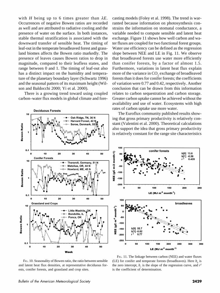
With regard to meteorology, FLUXNET can pro-vide new information on how the biosphere affectsthe partitioning of net radiation into sensible (H) andlatent heat (λE) exchange, as quantified by the Bowenratio. Figure 10 shows the yearly course in Bowen ra-tio for several selected sites. During the winter, theBowen ratio is variable, and in many instances large,

FIG. 8. Seasonal variation of initial quantum yield of a conifer(Scots) pine forest in Finland. Quantum yield is the initial slopeof the response between canopy CO

2 exchange and photosynthetic

photon flux density. PAR is photosynthetically active radiation.

FIG. 9. The relation between the optimum temperature forcanopy-scale gross primary productivity vs maximum meanmonthly air temperature during the summer growing season.These data show how photosynthesis adapts to climate. Here b(0)is the zero intercept and b(1) is the slope of the regression curve,and r2 is the coefficient of determination. Dashed lines are the stan-dard error of the regression at the 95% level.


with H being up to 6 times greater than λE.Occurrences of negative Bowen ratios are recordedas well and are attributed to radiative cooling and thepresence of water on the surface. In both instances,stable thermal stratification is associated with thedownward transfer of sensible heat. The timing ofleaf-out in the temperate broadleaved forest and grass-land biomes affects the Bowen ratio markedly. Thepresence of leaves causes Bowen ratios to drop inmagnitude, compared to their leafless states, andrange between 0 and 1. The timing of leaf-out alsohas a distinct impact on the humidity and tempera-ture of the planetary boundary layer (Schwartz 1996)and the seasonal pattern of its maximum height (Wil-son and Baldocchi 2000; Yi et al. 2000).

There is a growing trend toward using coupledcarbon–water flux models in global climate and fore-

casting models (Foley et al. 1998). The trend is war-ranted because information on photosynthesis con-strains the information on stomatal conductance, avariable needed to compute sensible and latent heatexchange. Figure 11 shows how well carbon and wa-ter fluxes are coupled for two functional forest groups.Water use efficiency can be defined as the regressionslope between NEE and LE in Fig. 11. We observethat broadleaved forests use water more efficientlythan conifer forests, by a factor of almost 1.5.Furthermore, variations in latent heat flux explainmore of the variance in CO

2 exchange of broadleaved

forests than it does for conifer forests; the coefficientsof variation were 0.77 and 0.42, respectively. Anotherconclusion that can be drawn from this informationrelates to carbon sequestration and carbon storage.Greater carbon uptake cannot be achieved without theavailability and use of water. Ecosystems with highrates of carbon uptake use more water.

The Euroflux community published results show-ing that gross primary productivity is relatively con-stant (Valentini et al. 2000). Theoretical calculationsalso support the idea that gross primary productivityis relatively constant for the range site characteristics

FIG. 10. Seasonality of Bowen ratio, the ratio between sensibleand latent heat flux densities, at representative deciduous for-ests, conifer forests, and grassland and crop sites.

FIG. 11. The linkage between carbon (NEE) and water fluxes(LE) for conifer and temperate forests (broadleaves). Here b

0 is

the zero intercept, b1 is the slope of the regression curve, and r2

is the coefficient of determination.

2430 Vol. 82, No. 11, November 2001

studied by the Euroflux network. The Euroflux data,however, come from a relatively narrow range of plantarchitectural and functional types (closed conifer anddeciduous forests) and climate conditions, so one canquestion how applicable the results may be across awider range of conditions. Using a biophysical model(Baldocchi and Meyers 1998), we predict that grossprimary productivity (GPP) of plants via photosynthe-sis is an asymptotic function of leaf area index, leafnitrogen, and the fraction of photosynthetically activeradiation that the canopy intercepts (Fig. 12).

There is a growing body of literature that is at-tempting to understand the impact of stand age oncarbon and water fluxes (Amiro et al. 1999; Schulzeet al. 1999; Law et al. 2001, manuscript submitted toGlobal Change Biol.; K. T. Paw U et al. 2001, manu-script submitted to Ecosystems). Productivity is as-sumed to diminish with age, and disturbances affectthe relative ratio between canopy carbon uptake andsoil respiration, and the ratio between canopy transpi-ration and soil evaporation. An attribute of a globalnetwork, such as FLUXNET, is the occurrence of siteswith similar species and functionality but differentages. Based on the data surveyed in Table 1, part d,we can draw the conclusion that the net carbon ex-change of old growth conifer forests is not carbonneutral (e.g., K. T. Paw U et al. 2001, manuscriptsubmitted to Ecosystems). A direct comparison of fluxdensities of carbon dioxide and water vapor that weremeasured over an old age Ponderosa pine stand in

Oregon (Metolius) and a young stand in northernCalifornia (Blodgett) are shown in Fig. 13. Peak ratesof evaporation are almost triple for the young stand,as compared to the old stand. Net daytime carbon as-similation fluxes of the young and old stands are outof phase during the summer growing season (seen at18 months in Fig. 13). The old stand is most produc-tive during the spring and autumn periods, while soilwater deficits restrict summertime rates of CO

2 up-

take. The young stand experiences greatest rates ofuptake during the summer, and peak rates of the youngstand can exceed peak rates of the old stand in thesummer by 14% (−140 g C m−2 month−1 near month30 vs −120 near month 18). Simulation modeling,which includes the effects of tree age, suggested thatthe milder winters and ample annual rainfall in theyoung stand allow it to have a higher leaf area thanthe old forest, allowing more carbon uptake throughthe year (Law et al. 2001, manuscript submitted toGlobal Change Biol.). Site management also has asubstantial impact on carbon and water fluxes at the

FIG. 12. The relation between gross primary productivity(GPP) and plant physiological capacity using field data and abiophysical model. The index of plant physiological capacity isa function of the maximum carboxylation velocity of photosyn-thesis (Vcmax), leaf area index (LAI), and the fraction of ab-sorbed visible sunlight ( f par). The Euroflux field data arereported in Valentini et al. (2000).

FIG. 13. The impact of stand age on daytime CO2 exchange

(NEE) and latent heat exchange (LE). The data are from a young(< 10 yr; black circles) and an old (> 200 yr; gray circles) pon-derosa pine forest (see Law et al. 2001, manuscript submittedto Global Change Biol.; Goldstein et al. 2000).


young site. The removal of understory shrubs in 1999reduced both CO

2 uptake and evaporation.

8. Conclusions

A global network of long-term measurement siteshas been established and is producing new informa-tion on how CO

2 and water vapor between the terres-

trial biosphere and atmosphere vary across a broadspectrum of biomes, climates, and timescales. The sci-ence generated so far indicates that rates of net car-bon uptake by tropical and temperate forests aresubstantial and exceed estimates previously generatedwith biospheric modeling systems. Gross primaryproductivity of forest ecosystems may not be constant,but may depend on plant architecture (e.g., on leafarea), foliage photosynthetic capacity, and the amountof sunlight absorbed.

Carbon net ecosystem exchange of broadleaveddeciduous forests strongly depends on length of grow-ing season, but is sensitive to perturbations such asdroughts, clouds, winter snow cover, and early thaw-ing, too. Concerning conifer forests, the conclusionsare not as unifying. Seasonal and annual sums of netcarbon exchange by boreal, semiarid, temperate, andhumid conifers differ among one another and fordifferent physiological reasons.

The response of canopy-scale CO2 exchange to

sunlight varies with cloud cover as clouds alter the di-rection of incoming sunlight and how it penetrates intoa canopy. The response of canopy-scale CO

2 exchange

to temperature is sensitive to the local climate. Thetemperature optima for canopy photosynthesis are dif-ferent for similar functional forest types in Europe andNorth America.

9. Future plans

The presence of sites on less than ideal terrain af-fords the micrometeorological community to take thechallenge and assess the impact of advection on themeasurement of long-term fluxes. Given the currenttower site distribution, there is a need to developtransect studies at anchor sites, so we can study spa-tial patterns in greater detail and better assess the im-pact of forest stand age, biodiversity, and landdisturbances. Aircraft flux studies can be used to aug-ment and extrapolate tower information in the spatial

domain. More physiological and stand structure stud-ies will be needed to aid in the interpretation of towermeasurements and to provide contextual informationto test ecophysiological models.

As data accumulate, new questions are arisingabout how to interpret fluxes made over mixed stands.Frontal passages cause the annual sums of ecosystemCO

2 exchange to be biased, as associated changes in

wind direction and speed cause a tower site to view adifferent flux footprint (Amiro 1998) or expose theecosystem to different temperature and humidity re-gimes. Over sites with inadequate fetch or mixed veg-etation in the flux footprint, flux densities that aremeasured will vary with wind direction. As knowl-edge evolves we may have to evaluate annual sumsby weighting field measurements on the basis of winddirection and the appropriate flux footprint probabil-ity density functions (Schmid 1994). On the flip side,we can use information from different wind directionsto address questions relating to the role of biodiver-sity on mass and energy exchange of ecosystems.

Acknowledgments. The FLUXNET project office and DataArchive is sponsored by NASA’s EOS Validation Program. Thecomponent regional networks and individual field sites are spon-sored by an array of government agencies. The Americas net-work, AmeriFlux, is sponsored by the United States Departmentsof Energy [Terrestrial Carbon Program, National Institutes ofGlobal Environmental Change (NIGEC)], Commerce (NOAA),and Agriculture (USDA/Forest Service), NASA, the NationalScience Foundation, and the Smithsonian Institution. These fed-eral agencies sponsor the Global Change Research Program(USGCRP) to promote cooperation with each other, academia,and the international community, in order to make it as easy aspossible for researchers and others to access and use globalchange data and information.

European sites in the Euroflux and Medeflu projects aresupported by the European Commission Directorate GeneralXII Environment and Climate Program. Canadian collabora-tors are sponsored by the Natural Sciences and EngineeringResearch Council of Canada (NSERC). Japanese and Asiansites are supported by the Ministry of Agriculture, Forest andFisheries (MAFF), the Ministry of Industrial Trade and Indus-try (MITI), and Ministry of Education, Science, Sports andCulture (MESSC).

We thank the numerous scientists, students, and techniciansresponsible for the day-to-day gathering of the flux data, andthe agency representatives who fund the respective projects.Without the dedicated efforts of so many individuals, this glo-bal network would not function or exist. Special appreciationis extended to Drs. Roger Dahlman, Diane Wickland, RuthReck, and David Starr, who have provided funds that supportedinitial planning workshops and that support many of the oper-ating science teams.

2432 Vol. 82, No. 11, November 2001

References

Amiro, B. D., 1998: Footprint climatologies for evapotranspi-ration in a boreal catchment. Agric. For. Meteor., 90, 195–201.

——, J. I. MacPherson, and R. L. Desjardins, 1999: BOREASflight measurements of forest-fire effects on carbon dioxideand energy fluxes. Agric. For. Meteor., 96, 199–208.

Amthor, J. S., 1995: Terrestrial higher-plant response to increas-ing atmospheric [CO

2] in relation to the global carbon cycle.

Global Change Biol., 1, 243–274.Amundson, R., L. Stern, T. Raisden, and Y. Wang, 1998: The

isotopic composition of soil and soil-respired CO2.

Geoderma, 82, 83–114.Anderson, D. E., S. B. Verma, and N. J. Rosenberg, 1984: Eddy

correlation measurements of CO2, latent heat and sensible heat

fluxes over a crop surface. Bound.-Layer Meteor., 29, 167–183.

Anthoni, P. M., B. E. Law, and M. H. Unsworth, 1999: Carbonand water vapor exchange of an open-canopied ponderosa pineecosystem. Agric. For. Meteor., 95, 115–168.

Aubinet, M., and Coauthors, 2000: Estimates of the annual netcarbon and water exchange of Europeran forests: TheEUROFLUX methodology. Adv. Ecol. Res., 30, 113–175.

BAHC Core Project Office, Eds., 1993: Biospheric aspects ofthe hydrological cycle. The operational plan. IGBP Rep. 27,Stockholm, Sweden, 103 pp.

Bakwin, P. S., P. P. Tans, D. F. Hurst, and C. L. Zhao, 1998:Measurements of carbon dioxide on very tall towers: Resultsof the NOAA/CMDL program. Tellus, 50B, 401–415.

Baldocchi, D. D., and T. P. Meyers, 1998: On using eco-physi-ological, micrometeorological and biogeochemical theory toevaluate carbon dioxide, water vapor and gaseous depositionfluxes over vegetation. Agric. For. Meteor., 90, 1–26.

——, B. B. Hicks, and T. P. Meyers, 1988: Measuring biosphere–atmosphere exchanges of biologically related gases with mi-crometeorological methods. Ecology, 69, 1331–1340.

——, R. Valentini, S. R. Running, W. Oechel, and R. Dahlman,1996: Strategies for measuring and modeling CO

2 and water

vapor fluxes over terrestrial ecosystems. Global Change Biol.,2, 159–168.

——, J. J. Finnigan, K. W. Wilson, K. T. Paw U, and E. Falge,2000: On measuring net ecosystem carbon exchange in com-plex terrain over tall vegetation. Bound.-Layer Meteor., 96,257–291.

——, E. Falge, and K. Wilson, 2001: A spectral analysis of bio-sphere–atmosphere trace gas flux densities and meteorologi-cal variables across hour to multi-year time scales. Agric.For. Meteor., 107, 1–27.

Barr, A. G., G. van der Kamp, R. Schmidt, and T. A. Black, 2000:Monitoring the moisture balance of a boreal aspen forest us-ing a deep groundwater piezometer. Agric. For. Meteor., 102,13–24.

Baumgartner, A., 1969: Meteorological approach to the exchangeof CO

2 between atmosphere and vegetation, particularly for-

ests stands. Photosynthetica, 3, 127–149.Berbigier, P., J.-M. Bonnefond, and P. Mellman, 2001: CO

2 and

water vapour fluxes for 2 years above Euroflux forest site.Agric. For. Meteor., 108, 183–197.

Betts, A. K., J. H. Ball, A. C. Beljaars, M. J. Miller, and P. A.Viterbo, 1996: The land surface–atmosphere interaction: Areview based on observational and global modeling perspec-tives. J. Geophys. Res., 101, 7209–7225.

Black, T. A., and Coauthors, 1996: Annual cycles of CO2 and

water vapor fluxes above and within a Boreal aspen stand.Global Change Biol., 2, 219–230.

——, W. J. Chen, A. G. Barr, M. A. Arain, Z. Chen, Z. Nesic,E. H. Hogg, H. H. Neumann, and P. C. Yang, 2000: Increasedcarbon sequestration by a boreal deciduous forest in yearswith a warm spring. Geophys. Res. Lett., 27, 1271–1274.

Canadell, J., and Coauthors, 2000: Carbon metabolism of theterrestrial biosphere. Ecosystems, 3, 115–130.

Ceulemans, R., and M. Mousseau, 1994: Tansley Review No.71. Effects of elevated atmospheric CO

2 on woody plants.

New Phytol., 127, 425–446.Ciais, P., P. P. Tans, M. Trolier, J. W. C. White, and R. J. Francy,

1995: A large North Hemisphere terrestrial CO2 sink indi-

cated by the 13C/12C ratio of atmospheric CO2. Science, 269,

1098–1102.Clark, K. L., H. L. Gholtz, J. B. Moncrieff, F. Cropley, and H.

W. Loescher, 1999: Environmental controls over net ex-changes of carbon dioxide from contrasting Florida ecosys-tems. Ecological Appl., 9, 936–948.

Conway, T. J., P. P. Tans, L. S. Waterman, K. W. Thoning, D. R.Kitzis, K. Masarie, and N. Zhang, 1994: Evidence for inter-annual variability of the carbon cycle from NOAA/CMDLglobal sampling network. J. Geophys. Res., 99, 22 831–22 855.

Cramer, W. J., D. W. Kicklighter, A. Bondeau, B. Moore III,G. Churkina, B. Nemry, A. Ruimy, and A. L. Schloss, 1999:Comparing global models of terrestrial primary productivity (NPP):Overview and key results. Global Change Biol., 5, 1–15.

Crawford, T. L., R. J. Dobosy, R. T. McMillen, C. A. Vogel, andB. B. Hicks, 1996: Air–surface exchange measurement in het-erogeneous regions: Extending tower observations with spa-tial structure observed from small aircraft. Global ChangeBiol., 2, 275–285.

Denmead, O. T., 1969: Comparative micrometeorology of awheat field and a forest of Pinus radiata. Agric. For. Meteor.,6, 357–371.

——, M. R. Raupach, F. X. Dunin, H. A. Cleugh, and R. Leuning,1996: Boundary layer budgets for regional estimates of scalarfluxes. Global Change Biol., 2, 255–264.

Denning, A. S., J. G. Collatz, C. Zhang, D. A. Randall, J. A. Berry,P. J. Sellers, G. D. Colello, and D. A. Dazlich, 1996: Simula-tions of terrestrial carbon metabolism and atmospheric CO

2 in

a general circulation model. Part 1: Surface carbon fluxes.Tellus, 48B, 521–542.

Desjardins, R. L., D. J. Buckley, and G. St. Amour, 1984: Eddyflux measurements of CO

2 above corn using a microcomputer

system. Agric. Meteor., 32, 257–265.——, and Coauthors, 1997: Scaling up flux measurements for the

boreal forest using aircraft-tower combinations. J. Geophys.Res., 102, 29 125–29 134.

Drake, B. G., M. A. Gonzalez-Meler, and S. P. Long, 1996: Moreefficient plants: A consequence of rising atmospheric CO

2?

Annu. Rev. Plant Physiol. Plant Mol. Biol., 48, 609–639.Falge, E., and Coauthors, 2001: Gap filling strategies for defen-

sible annual sums of net ecosystem exchange. Agric. For.Meteor., 107, 43–69.


Fan, S. M., M. Gloor, J. Mahlman, S. Pacala, J. Sarmiento,T. Takahashi, and P. Tans, 1998: A large terrestrial carbonsink in North America implied by atmospheric and oceaniccarbon dioxide data and models. Science, 282, 442–446.

Finnigan, J. J., 1999: A comment on the paper by Lee (1998):“On micrometeorological observations of surface–air ex-change over tall vegetation.” Agric. For. Meteor., 97, 55–64.

Foken, T., and B. Wichura, 1996: Tools for quality assessmentof surface-based flux measurements. Agric. For. Meteor.,78, 83–105.

Foley, J. A., S. Levis, I. C. Prentice, D. Pollard, and S. L. Th-ompson, 1998: Coupling dynamic models of climate and veg-etation. Global Change Biol., 4, 561–580.

Goldstein, A. H., and Coauthors, 2000: Effects of climate vari-ability on the carbon dioxide, water, and sensible heat fluxesabove a ponderosa pine plantation in the Sierra Nevada (CA).Agric. For. Meteor., 101, 113–129.

Goulden, M. L., J. W. Munger, S. M. Fan, B. C. Daube, and S. C.Wofsy, 1996a: Measurement of carbon storage by long-termeddy correlation: Methods and a critical assessment of ac-curacy. Global Change Biol., 2, 169–182.

——, ——, ——, ——, and ——, 1996b: Exchange of carbondioxide by a deciduous forest: Response to interannual climatevariability. Science, 271, 1576–1578.

——, and Coauthors, 1998: Sensitivity of boreal forest carbon bal-ance to soil thaw. Science, 279, 214–217.

Gower, S. T., C. J. Kucharik, and J. M. Norman, 1999: Direct andindirect estimation of leaf area index, fpar and net primary pro-duction of terrestrial ecosystems. Remote Sens. Environ., 70,29–51.

Granier, A., E. Ceschia, and C. Damesin, 2000: The carbon bal-ance of a young beech forest. Funct. Ecol., 14, 312–325.

Greco, S., and D. D. Baldocchi, 1996: Seasonal variations of CO2

and water vapor exchange rates over a temperate deciduousforest. Global Change Biol., 2, 183–198.

Gu, L., J. D. Fuentes, H. H. Shugart, R. M. Staebler, and T. A.Black, 1999: Responses of net ecosystem exchanges of car-bon dioxide to changes in cloudiness: Results from two NorthAmerican deciduous forests. J. Geophys. Res., 104, 31 421–31 434.

Halldin, S., S. E. Gryning, L. Gottschalk, A. Jochum, L.-C. Lundin,and A. A. Van de Griend, 1999: Energy, water and carbon ex-change in a boreal forest landscape—NOPEX experiences.Agric. For. Meteor., 98–99, 5–29.

Hanson, J. E., M. Sato, A. Lacias, R. Ruedy, I. Tegen, andE. Matthews, 1998: Climate forcings in the industrial era.Proc. Natl. Acad. Sci. USA. 95, 12 753–12 758.

Hollinger, D.Y., S. M. Goltz, E. A. Davidson, J. T. Lee, K. Tu,and H. T. Valentine, 1999: Seasonal patterns and environ-mental control of carbon dioxide and water vapor exchange inan ecotonal boreal forest. Global Change Biol., 5, 891–902.

Houghton, R. A., and G. Woodwell, 1980: The flax pond eco-system study: Exchanges of CO

2 between a salt marsh and

the atmosphere. Ecology, 61, 1434–1445.Inoue, I., 1958: An aerodynamic measurement of photosynthe-

sis over a paddy field. Proc. Seventh Japan National Con-gress of Applied Mechanics, 211–214.

Jacobs, C. M. J., and H. A. R. De Bruin, 1992: The sensitivityof transpiration to land-surface characteristics: Significanceof feedback. J. Climate, 5, 683–698.

Jarvis, P. G., G. B. James, and J. J. Landsberg, 1976: Conifer-ous forest. Vegetation and the Atmosphere, J. L. Monteith,Ed., Vol. 2, Academic Press, 171–240.

Kaimal, J. C., and J. J. Finnigan, 1994: Atmospheric BoundaryLayer Flows: Their Structure and Measurement. Oxford Uni-versity Press, 289 pp.

Kauppi, P. E., K. Mielikainen, and K. Kuuseia, 1992: Biomassand carbon budget of European forests, 1971 to 1990. Sci-ence, 256, 70–74.

Keeling, C. D., and T. P. Whorf, 1994: Atmospheric CO2 records

from sites in the SIO air sampling network. Trends ’93: Acompendium of data on global change. Oak Ridge NationalLaboratory Rep. ORNL/CDIAC-65, 16–26.

——, ——, M. Wahlen, and J. van der Plicht, 1995: Interannualextremes in the rate of rise of atmospheric carbon dioxidesince 1980. Nature, 375, 666–670.

——, S. C. Piper, and M. Heimann, 1996: Global and hemisphericCO

2 sinks deduced from changes in atmospheric O

2 concen-

tration. Nature, 381, 218–221.Kelliher, F. M., R. Leuning, M. R. Raupach, and E. D. Schulze,

1995: Maximum conductances for evaporation from globalvegetation types. Agric. For. Meteor., 73, 1–16.

Law, B. E., A. H. Goldstein, P. M. Anthoni, J. A. Panek, M. H.Unsworth, M. R. Bauer, J. M. Fracheboud, and N. Hultman,2000: CO

2 and water vapor exchange by young and old pon-

derosa pine ecosystems during a dry summer. Tree Physiol.,21, 299–308.

Lee, X., 1998: On micrometeorological observations of surface–air exchange over tall vegetation. Agric. For. Meteor., 91,39–50.

——, J. D. Fuentes, R. M. Staebler, and H. H. Neumann, 1999:Long-term observation of the atmospheric exchange of CO

2

with a temperate deciduous forest in southern Ontario, Canada.J. Geophys. Res., 104, 15 975–15 984.

Lemon, E. R., 1960: Photosynthesis under field conditions. II. Anaerodynamic method for determining the turbulent carbon di-oxide exchange between the atmosphere and a corn field.Agron. J., 52, 697–703.

Levy, P. E., A. Grelle, A. Lindroth, M. Molder, P. G. Jarvis,B. Kruijt, and J. B. Moncrieff, 1999: Regional scale CO

2 fluxes

over central Sweden by a boundary layer budget method.Agric. For. Meteor., 98–99, 169–180.

Lindroth, A., A. Grelle, and A. S. Moren, 1998: Long-term mea-surements of boreal forest carbon balance reveal large tempera-ture sensitivity. Global Change Biol., 4, 443–450.

Malhi, Y., A. D. Nobre, J. Grace, B. Kruijt, M. Pereira, A. Culf,and S. Scott, 1998: Carbon dioxide transfer over a centralAmazonian rain forest. J. Geophys. Res., 103, 31 593–31 612.

——, D. D. Baldocchi, and P. G. Jarvis, 1999: The carbon bal-ance of tropical, temperate and boreal forests. Plant, Cell andEnviron., 22, 715–740.

Markkanen, T., U. Rannik, P. Keronen, T. Suni, and T. Vesala,2001: Eddy covariance fluxes over a boreal Scots pine forest.Boreal Environ. Res., 6, 65–78.

Massman, W. J., 2000: A simple method for estimating fre-quency response corrections for eddy covariance systems.Agric. For. Meteor., 104, 185–198.

Meyers, T. P., 2001: A comparison of summertime water andCO

2 fluxes over rangeland for well-watered and drought con-

ditions. Agric. For. Meteor., 106, 205–214.

2434 Vol. 82, No. 11, November 2001

Moncrieff, J. B., Y. Mahli, and R. Leuning, 1996: The prop-agation of errors in long term measurements of land atmo-sphere fluxes of carbon and water. Global Change Biol., 2,231–240.

Monteith, J. L., and G. Szeicz, 1960: The CO2 flux over a field

of sugar beets. Quart. J. Roy. Meteor. Soc., 86, 205–214.Moore, C. J., 1986: Frequency response corrections for eddy co-

variance systems. Bound.-Layer Meteor., 37, 17–35.Myneni, R. B., C. D. Keeling, C. J. Tucker, G. Asrar, and R. R.

Nemani, 1997a: Increased plant growth in the northern highlatitudes from 1981–1991. Nature, 386, 698–702.

——, R. R. Nemani, and S. W. Running, 1997b: Estimation ofglobal leaf area index and absorbed par using radiative trans-fer models. IEEE Trans. Geosci. Remote Sens., 35, 1380–1393.

Niinemets, U., V. Oja, and O. Kull, 1999: Shape of leaf pho-tosynthetic electron transport versus temperature responsecurve is not constant along canopy light gradients in tem-perate deciduous trees. Plant, Cell Environ., 22, 1497–1513.

Norby, R. J., S. D. Wullschleger, C. A. Gunderson, D. W.Johnson, and R. Ceulemans, 1999: Tree responses to risingCO

2 in field experiments: Implication for the future forest.

Plant, Cell Environ., 22, 683–714.Oechel, W. C., G. L. Vourlitis, S. J. Hastings, R. C. Zulueta,

L. Hinzman, and D. Kane, 2000: Acclimation of ecosystemCO

2 exchange in the Alaskan Arctic in response to decadal

climate warming. Nature, 406, 978–981.Ohtaki, E., 1984: Application of an infrared carbon dioxide and

humidity instrument to studies of turbulent transport. Bound.-Layer Meteor., 29, 85–107.

Pielke, R. A., R. Avissar, M. Raupach, A. J. Dolman, X. Zeng,and A. S. Denning, 1998: Interactions between the atmosphereand terrestrial ecosystems: Influence on weather and climate.Global Change Biol., 4, 461–475.

Pilegaard, K., P. Hunnelshøj, N. O. Jensen, and Z. Chen, 2001:Two years of continuous CO

2 eddy-flux measurements over a

Danish beech forest. Agric. For. Meteor., 107, 29–41.Potosnak, M. J., S. C. Wofsy, A. S. Denning, T. J. Conway, J. W.

Munger, and D. H. Barnes, 1999: Influence of biotic exchangeand combustion sources on atmospheric CO

2 concentrations

in New England from observations at a forests flux tower. J.Geophys. Res., 104, 9561–9569.

Randerson, J. T., M. V. Thompson, T. J. Conway, I. Y. Fung, andC. B. Field, 1997: The contribution of terrestrial sources andsinks to trends in the seasonal cycle of atmospheric carbondioxide. Global Biogeochem. Cycles, 11, 535–560.

Raupach, M. R., and B. J. Legg, 1984: The uses and limitationsof flux-gradient relationships in micrometeorology. Agric.Water Manage., 8, 119–131.

Ruimy, A., P. G. Jarvis, D. D. Baldocchi, and B. Saugier, 1995:CO

2 fluxes over plant canopies and solar radiation: A review.

Adv. Ecol. Res., 26, 1–53.Running, S. W., D. D. Baldocchi, D. Turner, S. T. Gower,

P. Bakwin, and K. Hibbard, 1999: A global terrestrial moni-toring network, scaling tower fluxes with ecosystem model-ing and EOS satellite data. Remote Sens. Environ., 70, 108–127.

Schmid, H. P., 1994: Source areas for scalars and scalar fluxes.Bound.-Layer Meteor., 67, 293–318.

——, C. S. Grimmond, F. Cropley, B. Offerle, and H.-B. Su,2000: Measurements of CO

2 and energy fluxes over a mixed

hardwood forest in the mid-western United States. Agric. For.Meteor., 103, 357–374.

Schulze, E. D., and Coauthors, 1999: Productivity of forestsin the Eurosiberian boreal region and their potential to actas a carbon sink—A synthesis. Global Change Biol., 5, 703–722.

Schwartz, M. D., 1996: Examining the spring discontinuity indaily temperature ranges. J. Climate, 9, 803–808.

Sellers, P. J., and Coauthors, 1997: BOREAS in 1997: Scien-tific results, experimental overview and future directions. J.Geophys. Res., 102, 28 731–28 770.

Suyker, A. E., and S. B. Verma, 2001: Year-round observationsof the net ecosystem exchange of carbon dioxide in a nativetall grass prairie. Global Change Biol., 3, 279–290.

Tans, P. P., I. Y. Fung, and T. Takahashi, 1990: Observationalconstraints on the global atmospheric CO

2 budget. Science,

247, 1431–1438.Valentini, R., P. de Angelis, G. Matteucci, R. Monaco, S. Dore,

and G. E. Scarascia-Mugnozza, 1996: Seasonal net carbondioxide exchange of a beech forest with the atmosphere. Glo-bal Change Biol., 2, 199–208.

——, G. Matteucci, and A. J. Dolman, 2000: Respiration as themain determinant of carbon balance in European forests. Na-ture, 404, 861–864.

Verma, S. B., D. D. Baldocchi, D. E. Anderson, D. R. Matt, andR. E. Clement, 1986: Eddy fluxes of CO

2 water vapor, and

sensible heat over a deciduous forest. Bound.-Layer Meteor.,36, 71–91.

——, J. Kim, and R. J. Clement, 1989: Carbon dioxide, watervapor and sensible heat fluxes over a tall grass prairie.Bound.-Layer Meteor., 46, 53–67.

Vermetten, A. W. M., L. Ganzeveld, A. Jeuken, P. Hofschreuder,and G. M. J. Mohren, 1994: CO

2 uptake by a stand of Douglas

fir: Flux measurements compared with model calculations.Agric. For. Meteor., 72, 57–80.

Wilson, K. B., and D. D. Baldocchi, 2000: Esimating annual netecosystem exchange of carbon over five years at a deciduousforest in the southern United States. Agric. For. Meteor., 100,1–18.

——, ——, and P. J. Hanson, 2000: Spatial and seasonal vari-ability of photosynthesis parameters and their relationship toleaf nitrogen in a deciduous forest. Tree Physiol., 20, 787–797.

Wofsy, S. C., M. L. Goulden, J. W. Munger, S. M. Fan, P. S.Bakwin, B. C. Daube, S. L. Bassow, and F. A. Bazzaz, 1993:Net exchange of CO

2 in a mid-latitude forest. Science, 260,

1314–1317.Yamamoto, S., S. Murayama, N. Saigusa, and H. Kondo, 1999:

Seasonal and interannual variation of CO2 flux between a tem-

perate forest and the atmosphere in Japan. Tellus, 51B, 402–413.

Yi, C., K. J. Davis, P. S. Bakwin, B. W. Berger, and L. C. Marr,2000: Influence of advection on measurements of the net eco-system–atmosphere exchange of CO

2 from a very tall tower.

J. Geophys. Res., 105, 9991–9999.

fluxnet: a new tool to study the temporal and spatial

Documents