Munich Personal RePEc Archive

Follow the Value Added: Tracking

Bilateral Relations in Global Value

Chains

Borin, Alessandro and Mancini, Michele

Bank of Italy, Bank of Italy

14 November 2017

Online at https://mpra.ub.uni-muenchen.de/82692/

MPRA Paper No. 82692, posted 17 Nov 2017 11:31 UTC

Follow the Value Added:

Tracking Bilateral Relations in Global Value

Chains

Alessandro Borin and Michele Mancini*

(first version June 2015, this version November 2017)

Abstract

Following the spread of global value chains new statistical tools, the Inter-

Country Input-Output tables, and new analytical frameworks have been recently

developed to provide an adequate representation of supply and demand linkages

among the economies. Koopman, Wang and Wei propose an innovative accounting

methodology to decompose a country’s total gross exports by source and final des-

tination of their embedded value added. However this decomposition presents some

limitations and relevant inexactnesses in some of its components. We develop their

approach further by deriving a fully consistent counterpart for bilateral trade flows,

also at the sectoral level, addressing the main shortcomings of previous works. We

also provide correct breakdown of the foreign content in total (world) trade flows

and a brand new classification of these components that take the perspective of the

exporting country. Finally, drawing on our methodology we derive for the first time a

precise measure of international trade generated within global production networks.

Two examples of empirical applications with relevant policy implications are also

provided.

Keywords: global value chains; input-output tables; trade in value added; trade elasticity.

JEL classification: E16, F1, F14, F15.

*Bank of Italy. alessandro.borin@bancaditalia.it, michele.mancini@bancaditalia.it.

This paper is a revised and updated version of Borin, A. and M. Mancini, 2015. ‘Follow the Value

Added: bilateral gross export accounting’, Economic Working Papers, Bank of Italy. Section 2.4

has been added in May 2016, see Borin, A. and M. Mancini, 2016. ‘Participation in Global Value

Chains: measurement issues and the place of Italy’, Rivista di Politica Economica. Section 2.3 is

brand new. We thank Rita Cappariello, Riccardo Cristadoro, Stefano Federico, Alberto Felettigh,

Robert Johnson and Julia Wörz for insightful comments. The views expressed in this paper are

solely those of the authors and do not involve the responsibility of the Bank of Italy. The usual

disclaimer applies.

1

1 Introduction

The international fragmentation of production processes has challenged the capability of the stan-

dard trade statistics to truly represent supply and demand linkages among economies. In general

bilateral exports differ from the portion of a country’s GDP related with the production of goods

and services shipped to a certain outlet market. On one hand exports also embed imported inter-

mediate inputs, on the other hand the directly importing country often differs from the ultimate

destination where the good is absorbed by final demand. Whenever production is organized in se-

quential processing stages in different countries, trade statistics repeatedly double-count the same

value added. The diffusion of global value chains (GVC) has therefore deepened the divergence

between gross flows, as recorded by traditional trade statistics, and the data on production and

final demand as accounted for in statistics based on value added (above all GDP). Moreover, own

to the spread of GVC, new relevant questions regarding the role of countries and sectors in the

international markets have emerged. In particular, it has become crucial to assess the level of

participation of countries and sectors into the international sharing of production.

New data, as the Inter-Country Input-Output tables, and new analytic methodologies

have been developed in order to address these issues. Among the latter Koopman, Wang and Wei

(2014) (hereafter KWW) propose a comprehensive decomposition of total gross exports by the

source and destination of their embedded value added, that encompasses most of the methodologies

previously proposed in the literature (e.g. Hummels et al. 2001; Daudin et al., 2009; and Johnson

and Noguera, 2012). KWW point out that different schemes of international fragmentation of

production yield different proportions of value added content in gross exports. In particular, they

show that not all the double-counted flows in gross trade statistics are alike.

More specifically, KWW break gross exports down into different components of domestic

and foreign value added plus two items of “pure” double counting. As to the latter, they show

that gross exports do not in general consist only of value added that can be traced back to GDP

generated either at home or abroad. Instead, some trade flows are purely double-counted, as

when intermediate inputs cross a country’s borders several times according to the different stages

of production.1 It is worth noting that these double-counted items are increasingly important in

international trade flows (see Wang et al., 2013 and Cappariello and Felettigh, 2015), making the

KWW approach particularly valuable.

Albeit providing useful insights, the original KWW decomposition still presents some

relevant shortcomings and limitations. They correctly measure the total domestic value added in

exports, but the breakdown by destination market is imprecise. Furthermore their measures of

the value added generated abroad and of the foreign double counted items in total exports are

incorrect, since they overstate the latter component.2 More in general the KWW decomposition

finds limited scope for empirical applications since it neglects the bilateral and sectoral dimensions

of trade flows. It means, for instance, that it can not be applied to analyze all the direct and

indirect linkages between countries and sectors within the production networks. Another relevant

limitation is that we can not get a precise measure of the share of total trade that is related to

1A more detailed account of this mechanism is provided in section 2.2, where we discuss thedifferences between the sink and the source approaches of the bilateral decomposition.

2In section 2.2 we provide more detailed explanations of the shortcomings that affect the KWWdecomposition.

2

GVC participation from the standalone application of the KWW decomposition.

Besides these issues there are several other reasons why we might be interested in tracing

value added flows between countries. In fact firms trade with bilateral partners, even when par-

ticipating in more complex multi-country production networks. In studying GVC, it is relevant to

analyze the overall structure of production networks and to identify all the international and inter-

sectoral links. Methodologies like KWW’s can track the value added linkages between the country

of origin and the final destination. But we may also be interested in the position of a country (or

a sector) within the production process and in identifying its direct upstream and downstream

trade partners. This might be relevant in order to map geographically the production networks

and to analyze the international propagation of macroeconomic shocks, as exchange rates’ varia-

tions. Deepening the knowledge of these mechanisms also provides useful insights to interpret the

short-term dynamics of trade flows.3 Moreover, countries’ participation in GVCs affects bilateral

trade balances (Nagengast and Stehrer, 2016); this and other features of bilateral shipments, as

their merchandise composition, unambiguously influence trade policies (e.g. international trade

and investment agreements). More in general, the potential policy implications of all the aspects

mentioned above are clearly significant.

Our aim is to extend KWW’s methodology in order to obtain a consistent decomposition

of bilateral (and sectoral) trade flows that offers additional information on a good many matters

that cannot be investigated using simple gross trade data or aggregate trade in value added. For

instance, by considering the bilateral dimension of trade-production relations it is possible to

measure the amount of trade generated within global production networks.

We also intend to overcome shortcomings and limitations that affect the KWW decomposi-

tion and other previous attempts to get a bilateral counterpart of the KWW scheme. In particular

we provide proper definitions for some components that are incorrectly specified by KWW: i) the

domestic value added that is directly (and indirectly) absorbed by the final demand of the import-

ing country; ii) the foreign value added (FVA) in exports; iii) the double counted items produced

abroad. At the world level our corrected variant of the KWW’s FVA component resembles the

measure proposed by Johnson (2017), which is derived in a completely different framework. Indeed

the two measures do not coincide when computed for a single exporting country.4

Beside improving the measures of FVA and foreign double counted (FDC) within the

KWW framework, we also propose a completely alternative approach to split these two compo-

nents. According to the KWW logic, which in this aspect is shared also by Johnson (2017), FVA

and FDC are defined referring to world trade flows.5 However, from the perspective a particular

3Although ICIO data are only available with a lag, we can still use these tools to interpretand project short-term developments in international trade, insofar as the value added structureof bilateral exports is quite persistent over time. For example, if we know that in motor vehiclesmanufacturing a considerable share of the intermediate components exported from Italy to Ger-many are used to produce cars for the North American market, we presume that a slackening ofUS demand is likely to result in a reduction in shipments of parts from Italy to Germany.

4We also present an extended version of the FVA indicator proposed by Johnson (2017), witha breakdown by country of ultimate destination.

5In KWW a certain component of value added embedded in another country’s exports isrecorded as FVA only once in all (world) trade flows. If along the value chain the same componentcrosses several other borders, even of different countries, all these other times it is considered asforeign double counted. Note that this definition of double counted flows differs from that used for

3

exporting country this might not be economically meaningful and it produces an arbitrary allo-

cation of trade flows, depending on the number of upward (or downward) stages of production

that stand between the exporter and the country in which the value added was generated (or the

market of final destination). In order to address this issue we propose two brand new measures

of FVA and of FDC consistent with those adopted for the domestic content of exports. As better

explained later on, these measures can be derived in different ways for bilateral trade flows, then

generating distinct results at this level of disaggregation. Nevertheless, they all sum up to the

same indicators of FVA and of FDC when computed at the country level.

We also overcome the main problems that make imprecise and at least partially incorrect

the value added decompositions of bilateral exports previously proposed in the literature. In this

regard our work is related to that of Nagengast and Stehrer (2016) and Wang et al. (2013).

Nagengast and Stehrer (2016) point out that there are different ways to account value added

in bilateral trade. Indeed they propose two alternative methodologies: a first one takes the

perspective of the country where the value added originates (the source-based approach), a second

one takes the perspective of the country that ultimately absorbs it in final demand (the sink-based

approach). However, neither methodology in Nagengast and Stehrer (2016) are correctly specified,

so that they do not include the entire domestic value added embedded in each bilateral trade

flow. We propose two alternative breakdowns of bilateral exports that overcome this shortcoming,

while maintaining two separate frameworks for the source-based decomposition and for the sink-

based one. Both our decompositions correctly take into account the domestic value added, the

foreign value added and the double-counted components of bilateral exports. In both cases there

is a precise correspondence with the items in the KWW decomposition when we consider the

total exports of a country (apart from the components that are erroneously defined in KWW).

Having specific and internal consistent methodologies both for the sink-based and the source-based

approach allows to choose the most appropriate framework to the purpose of the analysis.

Wang et al. (2013) follow KWW closely and propose a single breakdown of bilateral

exports that can be exactly mapped into the original KWW decomposition summing all the export

flows across the destinations. This also means that the drawbacks of the KWW methodology

mentioned above apply also this bilateral variant (e.g. the incorrect identification of of the foreign

value added component). Moreover, Wang et al. (2013) mix sink and source approaches to

single out the different components, so that their methodology suffers from internal inconsistency.

Finally and more importantly, they can not identify the trade flows that are generated within

global supply networks, which has emerged as a key question in the literature. According to the

definition first proposed by Hummels et al. (2001) and commonly acknowledged in this field,

GVC schemes should entail at least two separate production stages in different countries, before

the good is ultimately shipped toward the final market. In other words there should be at least a

re-shipment of intermediate or final goods toward a third country (or back to the country of origin).

Conversely, ‘traditional’ production and trade patterns result in goods and services produced in a

certain country and consumed by the direct importer. Wang et al. (2013) methodology, which in

part follows a sink-based approach, does not allow to distinguish between these two cases, while

our source-based decomposition is suited to tackle this issue. Indeed in section 3.2 we propose

for the first time a measure of GVC-related trade that is consistent with Hummels et al. (2001)

the items produced domestically, which KWW consider as double counted only when they crossthe same national border more than once.

4

definition, providing empirical evidence about its evolution at the global level.

While we show a couple of possible implementations of our decompositions by using ICIO

tables (the World Input Output Database, WIOD, and the OECD-WTO Trade in Value Added,

TiVA) the detailed breakdown of bilateral/sectoral gross exports presented here might find a much

broader scope for empirical investigations on global production networks. In particular, it provides

the basic information needed to assess country/sector position and participation in GVCs and to

develop measures about the overall lengths of international supply chains (Antràs and Chor, 2013;

Wang et al., 2016; Borin and Mancini, 2016). In this way it will be possible to investigate at the

macro (country-sector) level some features of production networks that have emerged from case

studies (Dedrick et al., 2010; Ivarsson and Alvstam, 2011) and firm level analyses (Sturgeon et

al., 2008, Brancati et al., 2017).

The rest of the paper is organized as follows. The second section recalls KWW’s account-

ing, presents two novel decompositions of bilateral exports that overcome the main drawback in

KWW’s methodology, proposes an alternative approach to account for the foreign value added in

exports, illustrates how to include three different sectoral dimensions in the decompositions and

discusses how these new tools can contribute to analyze international production networks. The

third section shows two empirical applications: the first one adopts the sink-based approach to

explore the forward linkages of the world’s largest exporters; the second one takes the source-based

perspective to derive a measure of GVC-related trade and to assess how its evolution since the

mid-1990s has affected the relationship between world trade and income. Section four concludes.

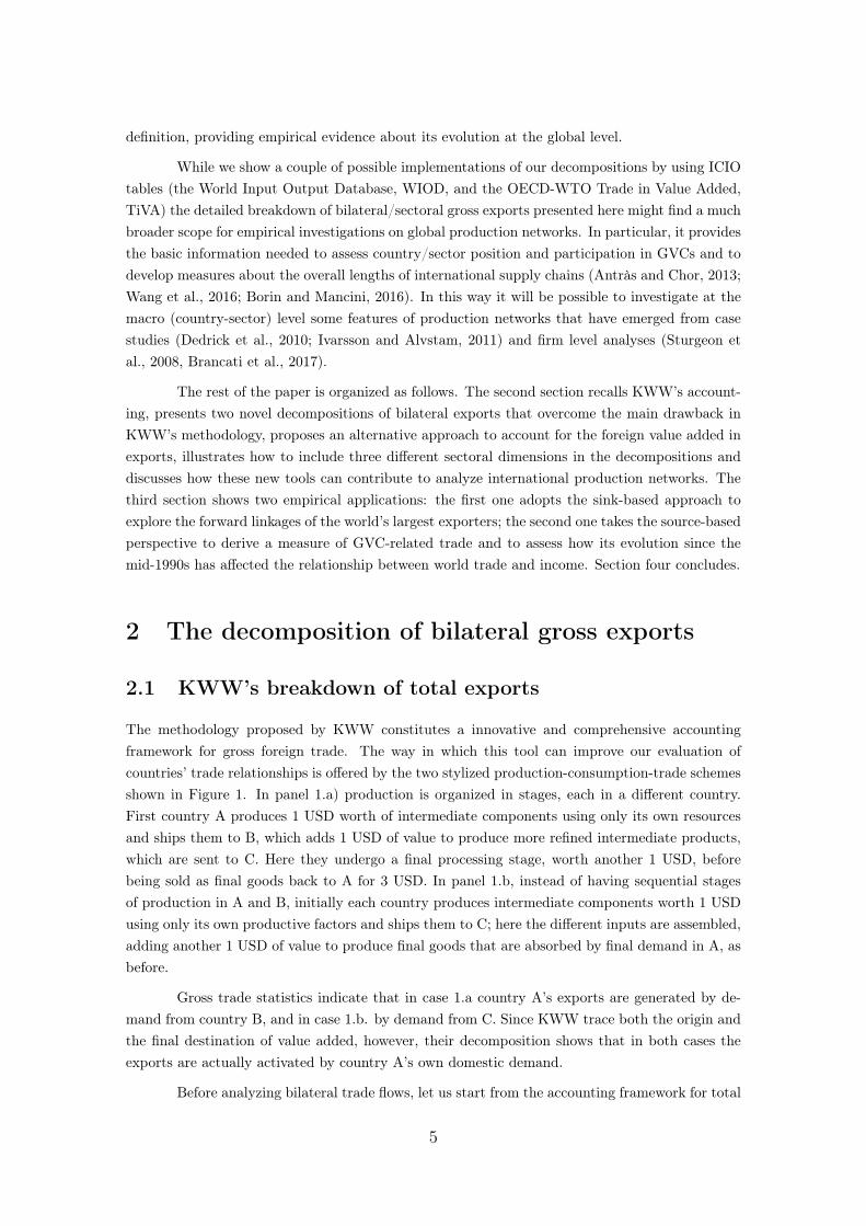
2 The decomposition of bilateral gross exports

2.1 KWW’s breakdown of total exports

The methodology proposed by KWW constitutes a innovative and comprehensive accounting

framework for gross foreign trade. The way in which this tool can improve our evaluation of

countries’ trade relationships is offered by the two stylized production-consumption-trade schemes

shown in Figure 1. In panel 1.a) production is organized in stages, each in a different country.

First country A produces 1 USD worth of intermediate components using only its own resources

and ships them to B, which adds 1 USD of value to produce more refined intermediate products,

which are sent to C. Here they undergo a final processing stage, worth another 1 USD, before

being sold as final goods back to A for 3 USD. In panel 1.b, instead of having sequential stages

of production in A and B, initially each country produces intermediate components worth 1 USD

using only its own productive factors and ships them to C; here the different inputs are assembled,

adding another 1 USD of value to produce final goods that are absorbed by final demand in A, as

before.

Gross trade statistics indicate that in case 1.a country A’s exports are generated by de-

mand from country B, and in case 1.b. by demand from C. Since KWW trace both the origin and

the final destination of value added, however, their decomposition shows that in both cases the

exports are actually activated by country A’s own domestic demand.

Before analyzing bilateral trade flows, let us start from the accounting framework for total

5

exports introduced by Koopman, Wang and Wei (2014). Their methodology is based on a global

input-output model with G countries and N sectors (for details see Appendix A which also gives

an exhaustive definition of our notation, which is essentially identical to KWW). Here let us only

recall that Ysr indicates the demand vector of final goods produced in s and consumed in r, B

is the global Leontief inverse matrix for the entire inter-country model, A is the global matrix of

input coefficients, Vs incorporates the value added shares embedded in each unit of gross output

produced by country s, Es∗ is the vector of total exports of country s for the N sectors, and uN

is the 1×N unit row vector.

The essential decomposition of total exports of country s (uNEs∗) in KWW is summarized

by the following accounting relationship:

uNEs∗ =

Vs

G∑

r 6=s

BssYsr +Vs

G∑

r 6=s

BsrYrr +Vs

G∑

r 6=s

G∑

t 6=s,r

BsrYrt

+

Vs

G∑

r 6=s

BsrYrs +Vs

G∑

r 6=s

BsrArs(I−Ass)−1

Yss

+ Vs

G∑

r 6=s

BsrArs(I−Ass)−1

Es∗

+

G∑

t 6=s

G∑

r 6=s

VtBtsYsr +

G∑

t 6=s

G∑

r 6=s

VtBtsAsr(I−Arr)−1

Yrr

+

G∑

t 6=s

G∑

r 6=s

VtBtsAsr(I−Arr)−1

Er∗ (1)

KWW defines the nine items in equation (1) as follows:

1. Vs

∑G

r 6=s BssYsr: domestic value added in direct final goods exports;

2. Vs

∑G

r 6=s BsrYrr: domestic value added in intermediate exports absorbed by direct im-

porters;

3. Vs

∑G

r 6=s

∑G

t 6=s,r BsrYrt: domestic value added in intermediate goods re-exported to third

countries;

4. Vs

∑G

r 6=s BsrYrs: domestic value added in intermediate exports reimported as final goods;

5. Vs

∑G

r 6=s BsrArs(I−Ass)−1

Yss: domestic value added in intermediate inputs reimported

as intermediate goods and finally absorbed at home;

6. Vs

∑G

r 6=s BsrArs(I−Ass)−1

Es∗: double-counted intermediate exports originally produced

at home;

7.∑G

t 6=s

∑G

r 6=s VtBtsYsr: foreign value added in exports of final goods;

8.∑G

t 6=s

∑G

r 6=s VtBtsAsr(I−Arr)−1

Yrr: foreign value added in exports of intermediate goods;

9.∑G

t 6=s

∑G

r 6=s VtBtsAsr(I−Arr)−1

Er∗: double-counted intermediate exports originally pro-

duced abroad.

6

Although KWW’s methodology allows to improve the knowledge of value added content

of total exports, it provides no insight into the structure of single bilateral flows. As already

mentioned, from a policy perspective this could be relevant for several reasons. Consider, for

example, the assessment of bilateral trade balances. In Figure 1.a A runs a 1 USD surplus with

B and a 3 USD deficit with C, all evaluated in terms of gross trade flows; in case 1.b, A shows a

net bilateral balance of -2 USD towards C and zero with respect to B. However, in value added

terms, A has a net trade deficit position of 1 USD with B and C in both panels. Thus while A’s

overall deficit is exactly the same in value added as in gross terms (2 USD), its bilateral positions

differ considerably between the two accounting methods. Using basic accounting relationships

and inter-country I-O tables, we can compute the bilateral positions in value added terms.6 Yet

this is not enough to disentangle the international production linkages and the ultimate demand

forces that generate a particular surplus/deficit between two countries in gross terms; nor does the

original KWW breakdown shed light on these matters when multiple trade partners and sources

of final demand are involved.

Moreover some of KWW’s definitions are questionable and, to some extent, incorrect, but

this will become clear by going though the analysis of bilateral trade flows, so we prefer to discuss

these issues in the following sections.

C

VA=1

B

VA=1

A

VA=1 Y=3

3 1

2

(1.a)

C

VA=1

B

VA=1

A

VA=1 Y=3

1

1

3

(1.b)

Figure 1: Value added versus gross export accounting of bilateral trade balances

2.2 The decomposition of bilateral trade

By focusing on bilateral trade flows we can follow the pattern of value added in exports along

the different phases of the value chain. However the input-output framework potentially allows

for infinite rounds of production. Hence we face a trade-off between adding details about the

international production linkages and providing an analytically tractable and conceptually intel-

ligible framework. Our compromise is to track the direct importing country, then - if the value

added is not absorbed there - we consider the additional destinations of re-export from the direct

importers.

6See equation (A.7) in Appendix A.

7

In summary, our strategy is to decompose gross bilateral trade flows identifying the fol-

lowing actors: i) the country of origin of value added; ii) the direct importers; iii) the (eventual)

second destination of re-export; iv) the country of completion of final products; v) the ultimate

destination market.

C

VA=0 Y=3

B

VA=1

A

VA=1+1=2

3 1

2

Figure 2: Value added and double counting in bilateral trade flows

Another conceptual issue that arises in considering the single bilateral flows regards the

purely double counted items. As pointed out by Nagengast and Stehrer (2016), when a certain

portion of value added crosses the same border more than once it has to be assigned to a particular

gross bilateral trade flow, while it should be recorded as purely double counted in the other

shipments. The issue is clearly pointed out by the scheme reported in Figure 2: here the 1 USD of

value added originally produced in A is first exported to B as intermediate inputs, processed there,

then shipped back to A and used to produce final goods for re-export to C. In this case, the value

added generated in the very first stage of production in A is counted twice in its gross bilateral

exports to B and C. The question is the following: in which case should we consider it as ‘domestic

value added’ and in which as ‘double counted’? Nagengast and Stehrer (2016) point out that it

is an arbitrary choice and propose two alternative approaches: a first one takes the perspective of

the country where the value added originates (the source-based approach), a second one that of

the country that ultimately absorbs it in final demand (the sink-based approach). As regards the

example in Figure 2, according to the source-based approach the original 1 USD of production of

country A would be considered as ‘domestic value added’ in the gross exports to B (and ‘double

counted’ in the shipments to C); vice-versa using the sink-based approach it would be considered

as ‘domestic value added’ in the exports to C (and ‘double counted’ in the shipments to B).

In short we can say that the source-based method accounts the value added the first time

it leaves the country of origin, while the sink-based approach considers it the last time it crosses

the national borders. The choice between the two frameworks depends on the particular empirical

issue we want to address. For instance if one is interested in inquiring the trade linkages through

which the value added reaches a certain market of final destination, the sink-based approach is

probably more appropriate. On the contrary the source-based method allows to trace the very

first destination of value added from the country of origin. In section 3 we show two different

empirical applications, each one adopting one of the two approaches described above.

Hereafter we present two decompositions of bilateral trade flows. The first one follows

a sink-based approach, the second one a source-based logic. We show how our methodologies

8

address critical aspects of KWW and other previous contributions by Wang et al. (2013) and by

Nagengast and Stehrer (2016). In Appendix B we also provide the full analytical derivation for

the sink-based approach, which is the most complex.7

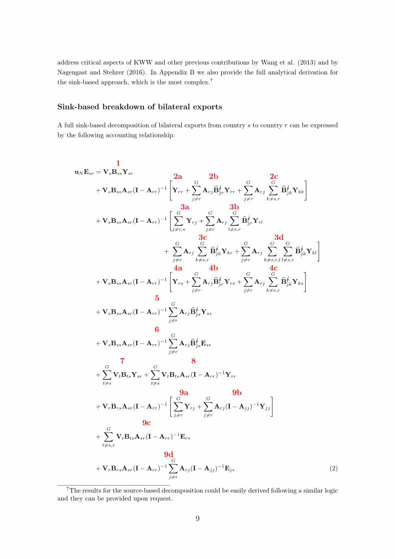
Sink-based breakdown of bilateral exports

A full sink-based decomposition of bilateral exports from country s to country r can be expressed

by the following accounting relationship:

uNEsr =

1VsBssYsr

+VsBssAsr(I−Arr)−1

[2a

Yrr +

2bG∑

j 6=r

ArjB✄sjrYrr +

2cG∑

j 6=r

Arj

G∑

k 6=s,r

B✄sjkYkk

]

+VsBssAsr(I−Arr)−1

[ 3aG∑

j 6=r,s

Yrj +

3bG∑

j 6=r

Arj

G∑

l 6=s,r

B✄sjrYrl

+

3cG∑

j 6=r

Arj

G∑

k 6=s,r

B✄sjkYkr +

3dG∑

j 6=r

Arj

G∑

k 6=s,r,l

G∑

l 6=s,r

B✄sjkYkl

]

+VsBssAsr(I−Arr)−1

[4a

Yrs +

4bG∑

j 6=r

ArjB✄sjrYrs +

4cG∑

j 6=r

Arj

G∑

k 6=s,r

B✄sjkYks

]

+

5

VsBssAsr(I−Arr)−1

G∑

j 6=r

ArjB✄sjsYss

+

6

VsBssAsr(I−Arr)−1

G∑

j 6=r

ArjB✄sjsEs∗

+

7G∑

t 6=s

VtBtsYsr +

8G∑

t 6=s

VtBtsAsr(I−Arr)−1

Yrr

+VrBrsAsr(I−Arr)−1

[ 9aG∑

j 6=r

Yrj +

9bG∑

j 6=r

Arj(I−Ajj)−1

Yjj

]

+

9cG∑

t 6=s,r

VtBtsAsr(I−Arr)−1

Er∗

+

9d

VrBrsAsr(I−Arr)−1

G∑

j 6=r

Arj(I−Ajj)−1

Ej∗ (2)

7The results for the source-based decomposition could be easily derived following a similar logicand they can be provided upon request.

9

where B✄s ≡ (I −A✄s)−1 is the Leontief inverse matrix derived from the input coefficient

matrix A✄s, which excludes the input requirement of other economies from country s:8

A✄s =

A11 A12 · · · A1s · · · A1G

......

. . ....

......

0 0 · · · Ass · · · 0

......

......

. . ....

AG1 AG2 · · · AGs · · · AGG

We can define the items that form the bilateral decomposition of gross exports as follows:

1 domestic value added (VA) in direct final good exports;

2a domestic VA in intermediate exports absorbed by direct importers as local final goods;

2b domestic VA in intermediate exports absorbed by direct importers as local final goods only

after additional processing stages abroad;

2c domestic VA in intermediate exports absorbed by third countries as local final goods;

3a domestic VA in intermediate exports absorbed by third countries as final goods from direct

bilateral importers;

3b domestic VA in intermediate exports absorbed by third countries as final goods from direct

bilateral importers only after further processing stages abroad;

3c domestic VA in intermediate exports absorbed by direct importers as final goods from third

countries;

3d domestic VA in intermediate exports absorbed by third countries as final goods from other

third countries;

4a domestic VA in intermediate exports absorbed at home as final goods of the bilateral

importers;

4b domestic VA in intermediate exports absorbed at home as final goods of the bilateral

importers after additional processing stages abroad;

4c domestic VA in intermediate exports absorbed at home as final goods of a third country;

5 domestic VA in intermediate exports absorbed at home as domestic final goods;

6 double-counted intermediate exports originally produced at home;

7 foreign VA in exports of final goods;

8 foreign VA in exports of intermediate goods directly absorbed by the importing country r;

9a and 9b foreign VA in exports of intermediate goods re-exported by r directly to the country of final

absorption.

9c and 9d double-counted intermediate exports originally produced abroad.

8In Appendix B we describe in detail how and for which purpose the B ✄s matrix is derived.

10

The enumeration of the items recalls the original KWW components, which can be ob-

tained as a simple summation over the importing countries r of the corresponding items in our

bilateral decomposition (e.g. the second term in KWW is equal to the sum across the r destina-

tions of 2a+2b+2c). A formal proof of this equivalence for each item in equation (2) is provided

in Appendix C.

We can now compare the definitions of the items here above with those originally assigned

by KWW, which have been quoted below equation (1). Despite the algebraical consistency be-

tween the two classifications, there are a few discrepancies, due to the shortcomings that affect

KWW’s methodology. First KKW do not properly allocate the domestic value added embedded

in intermediate exports between the share going to direct importers and the share absorbed in

third markets (see also Nagengast and Sterher, 2016 on the same point). Second, the terms 9a

and 9b of equation (2) are erroneously classified as double-counted by KWW. By correcting these

two distortions our breakdown of bilateral trade flows results also in a substantial refinement of

the original KWW classification of aggregate exports.

According to KWW, the first and second components of domestic value added of exports

go entirely to direct importers’ final demand. Using the decomposition of bilateral exports in

equation (2), we observe that only sub-items 2a and 2b are actually part of the direct importers’

final demand. Conversely, part of the third item (3c), which KWW classify as third countries’ final

demand, should be also considered as direct importers’ absorption of domestic VA. This makes the

total value added produced at home and finally absorbed by the bilateral trade partners equal to

the sum across destinations of: 1, 2a, 2b and 3c. This clearly differs from KWW’s definition (i.e.

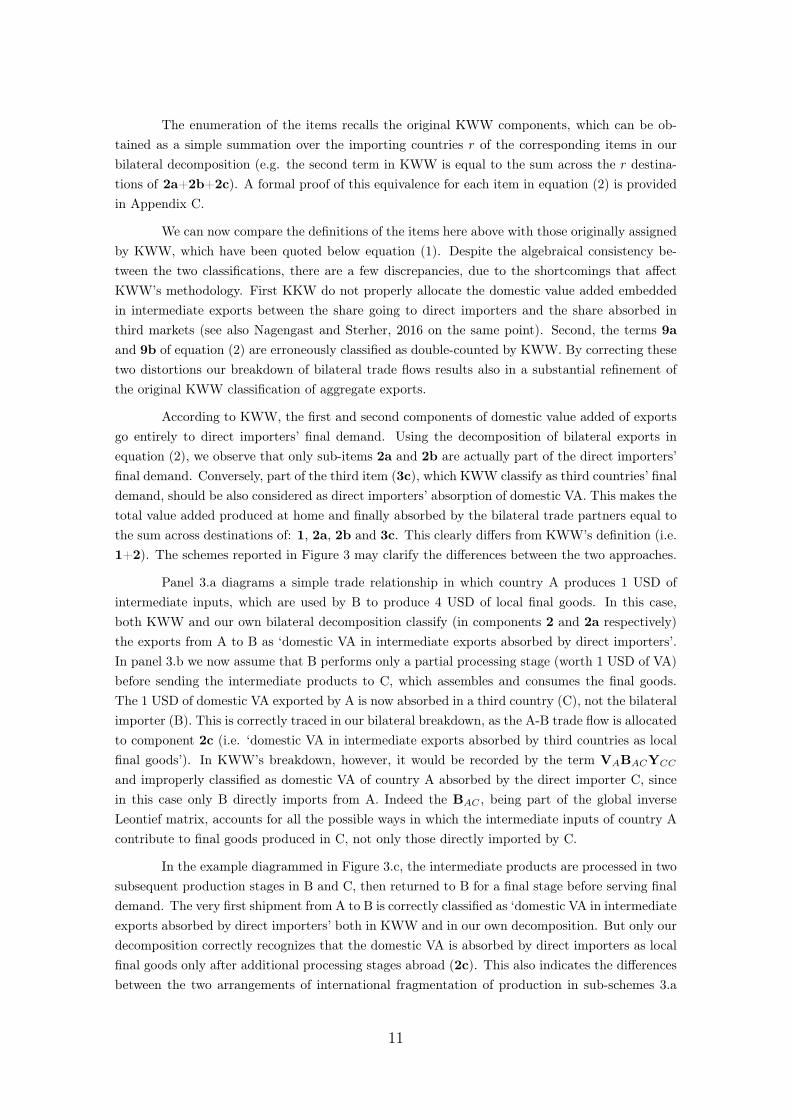
1+2). The schemes reported in Figure 3 may clarify the differences between the two approaches.

Panel 3.a diagrams a simple trade relationship in which country A produces 1 USD of

intermediate inputs, which are used by B to produce 4 USD of local final goods. In this case,

both KWW and our own bilateral decomposition classify (in components 2 and 2a respectively)

the exports from A to B as ‘domestic VA in intermediate exports absorbed by direct importers’.

In panel 3.b we now assume that B performs only a partial processing stage (worth 1 USD of VA)

before sending the intermediate products to C, which assembles and consumes the final goods.

The 1 USD of domestic VA exported by A is now absorbed in a third country (C), not the bilateral

importer (B). This is correctly traced in our bilateral breakdown, as the A-B trade flow is allocated

to component 2c (i.e. ‘domestic VA in intermediate exports absorbed by third countries as local

final goods’). In KWW’s breakdown, however, it would be recorded by the term VABACYCC

and improperly classified as domestic VA of country A absorbed by the direct importer C, since

in this case only B directly imports from A. Indeed the BAC , being part of the global inverse

Leontief matrix, accounts for all the possible ways in which the intermediate inputs of country A

contribute to final goods produced in C, not only those directly imported by C.

In the example diagrammed in Figure 3.c, the intermediate products are processed in two

subsequent production stages in B and C, then returned to B for a final stage before serving final

demand. The very first shipment from A to B is correctly classified as ‘domestic VA in intermediate

exports absorbed by direct importers’ both in KWW and in our own decomposition. But only our

decomposition correctly recognizes that the domestic VA is absorbed by direct importers as local

final goods only after additional processing stages abroad (2c). This also indicates the differences

between the two arrangements of international fragmentation of production in sub-schemes 3.a

11

B

VA=3 Y=4

A

VA=1

1

4

(3.a)

C

VA=2 Y=4

B

VA=1

A

VA=1

1

2

4

(3.b)

C

VA=1

B

VA=1+1=2

Y=4

A

VA=1

1

2

4

3

(3.c)

C

VA=2

B

VA=1 Y=4

A

VA=1

1

2

4

(3.d)

Figure 3: Accounting of the absorption of domestic value added of exports by directimporters

12

and 3.c.

Scheme 3.d differs from 3.c only in that the final assembly stage is performed in C rather

than B, which is still the country of final destination. As regards country A, B is both the direct

importer and the final demand absorber, so its exports to B should be considered as domestic VA

absorbed by a direct importer, which is how they are mapped in our decomposition (in item 3c),

whereas in KWW’s method they are allocated to third countries’ absorption of domestic VA of

exports.

The value added decomposition of bilateral trade flows offers useful information for valuing

trade balances between countries, reconciling the gross export data with value added accounting.

For instance, going back to the example in Figure 1, in case 1.a we see that the exports from

A to B are generated by A’s demand for C’s final goods, since they are classified in item 4c

of equation (2) (i.e. ‘domestic VA in intermediate exports absorbed at home as final goods

of a third country’). In example 1.b, instead, exports from A to C are classed under 4a (i.e.

‘domestic VA in intermediate exports absorbed at home as final goods of the bilateral importers’).

This differentiation, which is not envisaged in KWW’s original framework, gives insights into the

structure of international production and demand linkages, especially in dealing with the sort of

complex production networks that prevail in the real world.

Our sink-based decomposition summarized by equation (2) differs substantially also from

the one in Nagengast and Sterher (2016). In fact they classify as domestic value added absorbed

by direct importers only that embedded in goods that do not leave this country again, assigning

the remainder to the double counted component. In this way they do not take into account

what we have classified in the 2b and 3c components, underestimating the domestic value added

absorbed by direct importers. It means that, for instance, in the scheme 3.c and 3.d described

above, the exports from country A to country B would be entirely classified as double counted

in the decomposition of their bilateral flows. Also their definitions of the domestic value added

finally absorbed at home and by third countries turn out to be imprecise, leading in this case to

an overestimation of the domestic value added in exports. The scheme diagrammed in Figure 4

highlights this particular issue. In this case, two stages of production, each worth 1 USD of value

added, are performed both in country A and B, before the final good being shipped from B to the

destination market C. The total bilateral gross exports from A to B are equal to 4 USD, which

consist of 2 USD of VA generated in A, 1 USD of VA generated in B and 1 USD of double counted

VA, originated in the first stage of production in A and embedded in the second shipment from A

to B. In Nagengast and Sterher (2016) this 1 USD of double counted items would be assigned to

the domestic value added of A absorbed by third country C, overestimating this component.9 This

9This overestimation stems from the double use of the global inverse Leontief matrix in someof the terms of the decomposition of Nagengast and Sterher (2016). In fact in the exam-ple of Figure 4, the domestic value added absorbed in third countries would be calculated asVABAAAABBBBYBC (both in sink and source-based methodology). Since BAA accounts for allthe possible ways in which the intermediate inputs of country A contribute to the production inA, VABAA encompasses the entire value added of A generated both in the first and the secondstage of production. Then the VABAA matrix should be applied only to the second export flow toB, in order to extract A’s value added following the sink-based logic. Instead, since they accountthe B’s gross output necessary for the production of the final good exported to C through theBBB matrix, they are recording both the first and the second stage of production in B and henceboth the shipments of intermediate inputs from A. So they end up with an overestimation of the

13

drawback applies both to their sink and source-based decompositions. This inaccuracy in defining

some of the items entails that neither methodology proposed by Nagengast and Sterher (2016) can

retrieve the entire domestic value added exported by a country summing the corresponding items

across the bilateral flows. On the contrary both our sink-based decomposition and source-based

breakdown, shown below, meet this requirement.

C

VA=0 Y=4

B

VA=1+1=2

A

VA=1+1=2

1

2

3

4

Figure 4: Domestic value added and double counting with final destination in thirdcountries

Figure 4 can be also used to point out another relevant issue of KWW’s methodology and

of its bilateral version by Wang et al.(2013): the erroneous classification of part of the foreign

value added in exports (i.e. the exclusion of items 9a and 9b of equation (2) from the foreign

value added). KKW’s classification fail to record the VA originated in the upstream stages of the

production process by the country that exports to the market of final destination (i.e. country r).

We can make this point clearer by referring again to the scheme in figure 4. The 1 USD of value

added produced by B in the second production phase should be considered as FVA in country

A’s re-exports to B (i.e. the flow worth 3 USD), but in KWW’s classification this is recorded as

double counted, as B is not the market of final destination. Instead braking down A’s exports

according to equation (2) this component produced by B is correctly classified as foreign value

added (within term 9a).

Source-based breakdown of bilateral exports

The source-based decomposition of bilateral exports from country s to country r can be expressed

as follows:

uNEsr =

1a*Vs(I−Ass)

−1Ysr

+Vs(I−Ass)−1

Asr(I−Arr)−1

[ 1b*G∑

j 6=r

ArjBjsYsr +

1c*G∑

j 6=r

Arj

G∑

k 6=s,r

BjsYsk

]

VA produced in A.

14

+Vs(I−Ass)−1

Asr(I−Arr)−1

[2a*

Yrr +

2b*G∑

j 6=r

ArjBjrYrr +

2c*G∑

j 6=r

Arj

G∑

k 6=s,r

BjkYkk

]

+Vs(I−Ass)−1

Asr(I−Arr)−1

[ 3a*G∑

j 6=r,s

Yrj +

3b*G∑

j 6=r

Arj

G∑

l 6=s,r

BjrYrl

+

3c*G∑

j 6=r

Arj

G∑

k 6=s,r

BjkYkr +

3d*G∑

j 6=r

Arj

G∑

k 6=s,r,l

G∑

l 6=s,r

BjkYkl

]

+Vs(I−Ass)−1

Asr(I−Arr)−1

[4a*

Yrs +

4b*G∑

j 6=r

ArjBjrYrs +

4c*G∑

j 6=r

Arj

G∑

k 6=s,r

BjkYks

]

+

5*

Vs(I−Ass)−1

Asr(I−Arr)−1

G∑

j 6=r

ArjBjsYss

+

6*

Vs(I−Ass)−1

G∑

t 6=s

AstBtsEsr

+

G∑

t 6=s

Vt(I−Att)−1

Ats(I−Ass)−1

[7*

Ysr +

8*

Asr(I−Arr)−1

Yrr

]

+

9a*G∑

t 6=s

Vt(I−Att)−1

Ats(I−Ass)−1

Asr(I−Arr)−1

G∑

j 6=r

Yrj

+

9b*G∑

t 6=s

Vt(I−Att)−1

Ats(I−Ass)−1

Asr(I−Arr)−1

G∑

j 6=r

Arj

G∑

k

G∑

l

BjkYkl

+

G∑

t 6=s

Vt(I−Att)−1

[ 9c*G∑

j 6=t,s

AtjBjsEsr +

9d*

Ats(I−Ass)

G∑

t 6=s

AstBtsEsr

](3)

We can define the items above as:

1a* domestic value added (VA) in final good exports directly absorbed by bilateral importers;

1b* domestic VA in intermediate exports absorbed by bilateral importers as domestic final

goods after additional processing stages;

1c* domestic VA in intermediate exports absorbed by third countries as domestic final goods

after additional processing stages;

2a* domestic VA in intermediate exports absorbed by direct importers as local final goods;

2b* domestic VA in intermediate exports absorbed by direct importers as local final goods only

after further processing stages;

2c* domestic VA in intermediate exports absorbed by third countries as local final goods;

15

3a* domestic VA in intermediate exports absorbed by third countries as final goods from direct

bilateral importers;

3b* domestic VA in intermediate exports absorbed by third countries as final goods from direct

bilateral importers only after further processing stages;

3c* domestic VA in intermediate exports absorbed by direct importers as final goods from third

countries;

3d* domestic VA in intermediate exports absorbed by third countries as final goods from other

third countries;

4a* domestic VA in intermediate exports absorbed at home as final goods of the bilateral

importers;

4b* domestic VA in intermediate exports absorbed at home as final goods of the bilateral

importers after further processing stages;

4c* domestic VA in intermediate exports absorbed at home as final goods of a third country;

5* domestic VA in intermediate exports absorbed at home as domestic final goods;

6* double-counted intermediate exports originally produced at home;

7* foreign VA in exports of final goods;

8* foreign VA in exports of intermediate goods directly absorbed by the importing country r;

9a* and 9b* foreign VA in exports of intermediate goods re-exported by r;

9c* and 9d* double-counted intermediate exports originally produced abroad.

As for the sink-based decomposition, the enumeration of the items here above recalls

the original KWW components. However while for the domestic content (terms 1a* to 6*), the

correspondent KWW’s items can be obtained as a simple summation over the importing countries

r,10 this property does not hold for the foreign content part. At the level of the single exporter

terms 7* to 9d* differ from those proposed in the sink-based decomposition of equation (2)

because the notions of FVA and FDC in KWW are defined at world level (not at country level like

the DVA and the DDC). The source base classification of FVA and FDC of equation (3) follow a

similar logic.11 However while in the source-based approach a certain item is recorded as FVA the

first time that it is re-exported by a foreign country (and as FDC in all the other re-exports), in the

sink-based framework all the FVA is accounted the last time that it is embedded in a export flow.

Since the first re-exporter may not coincide with the last one, also the source-based indicators of

foreign content and the sink-based ones usually differ when computed at the level of the exporting

country. However both the approach account a given item as FVA only once in world trade flows.

It means that aggregating at the world level the FVA and FDC components of equation (2) and

(3) we obtain exactly the same measures. In section 2.3 we present an alternative approach to

classify the foreign double counted from the perspective of the exporting country that leads to a

unique measure of FVA and FDC both in a sink-based framework and in a source-based one.

10A formal proof is available upon request.11In particular the definition of FVA in (3) corresponds to the measure proposed by Johnson

(2017) disaggregated by country of final destination.

16

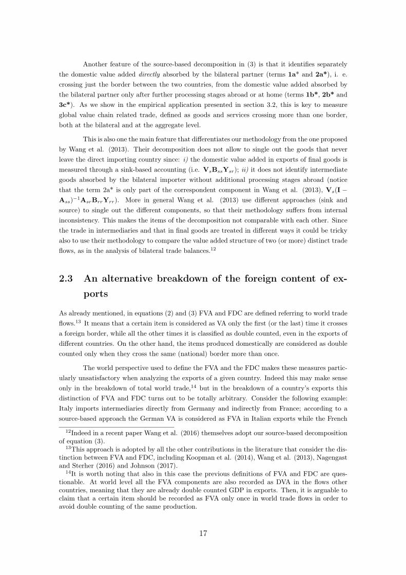
Another feature of the source-based decomposition in (3) is that it identifies separately

the domestic value added directly absorbed by the bilateral partner (terms 1a* and 2a*), i. e.

crossing just the border between the two countries, from the domestic value added absorbed by

the bilateral partner only after further processing stages abroad or at home (terms 1b*, 2b* and

3c*). As we show in the empirical application presented in section 3.2, this is key to measure

global value chain related trade, defined as goods and services crossing more than one border,

both at the bilateral and at the aggregate level.

This is also one the main feature that differentiates our methodology from the one proposed

by Wang et al. (2013). Their decomposition does not allow to single out the goods that never

leave the direct importing country since: i) the domestic value added in exports of final goods is

measured through a sink-based accounting (i.e. VsBssYsr); ii) it does not identify intermediate

goods absorbed by the bilateral importer without additional processing stages abroad (notice

that the term 2a* is only part of the correspondent component in Wang et al. (2013), Vs(I −

Ass)−1

AsrBrrYrr). More in general Wang et al. (2013) use different approaches (sink and

source) to single out the different components, so that their methodology suffers from internal

inconsistency. This makes the items of the decomposition not comparable with each other. Since

the trade in intermediaries and that in final goods are treated in different ways it could be tricky

also to use their methodology to compare the value added structure of two (or more) distinct trade

flows, as in the analysis of bilateral trade balances.12

2.3 An alternative breakdown of the foreign content of ex-

ports

As already mentioned, in equations (2) and (3) FVA and FDC are defined referring to world trade

flows.13 It means that a certain item is considered as VA only the first (or the last) time it crosses

a foreign border, while all the other times it is classified as double counted, even in the exports of

different countries. On the other hand, the items produced domestically are considered as double

counted only when they cross the same (national) border more than once.

The world perspective used to define the FVA and the FDC makes these measures partic-

ularly unsatisfactory when analyzing the exports of a given country. Indeed this may make sense

only in the breakdown of total world trade,14 but in the breakdown of a country’s exports this

distinction of FVA and FDC turns out to be totally arbitrary. Consider the following example:

Italy imports intermediaries directly from Germany and indirectly from France; according to a

source-based approach the German VA is considered as FVA in Italian exports while the French

12Indeed in a recent paper Wang et al. (2016) themselves adopt our source-based decompositionof equation (3).

13This approach is adopted by all the other contributions in the literature that consider the dis-tinction between FVA and FDC, including Koopman et al. (2014), Wang et al. (2013), Nagengastand Sterher (2016) and Johnson (2017).

14It is worth noting that also in this case the previous definitions of FVA and FDC are ques-tionable. At world level all the FVA components are also recorded as DVA in the flows othercountries, meaning that they are already double counted GDP in exports. Then, it is arguable toclaim that a certain item should be recorded as FVA only once in world trade flows in order toavoid double counting of the same production.

17

VA is classified as FDC, even if the two components contribute in very a similar way to the value

embedded in Italian exports.15 From the perspective of the exporting country, we are usually

interested in measuring the share of exports that can be traced back to the domestic GDP and

the share that corresponds to the foreign one, independently from the number of upstream or

downstream production stages that separate the exporter from the country of origin and/or the

market of final destination. To this aim we need a notion of foreign double counting that follow

the same logic adopted for the domestic double counting: we want to exclude from the FVA only

the items that cross the same (domestic) border more than once.

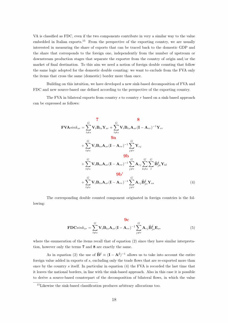
Building on this intuition, we have developed a new sink-based decomposition of FVA and

FDC and new source-based one defined according to the perspective of the exporting country.

The FVA in bilateral exports from country s to country r based on a sink-based approach

can be expressed as follows:

FVAsinksr =

7G∑

t 6=s

VtBtsYsr +

8G∑

t 6=s

VtBtsAsr(I−Arr)−1

Yrr

+

9aG∑

t 6=s

VtBtsAsr(I−Arr)−1

G∑

j 6=r

Yrj

+

9bG∑

t 6=s

VtBtsAsr(I−Arr)−1

G∑

j 6=r

Arj

G∑

k 6=s

G∑

l

B✄sjkYkl

+

9b’G∑

t 6=s

VtBtsAsr(I−Arr)−1

G∑

j 6=r

ArjB✄sjsYss (4)

The corresponding double counted component originated in foreign countries is the fol-

lowing:

FDCsinksr =

9cG∑

t 6=s

VtBtsAsr(I−Arr)−1

G∑

j 6=r

ArjB✄sjsEs∗ (5)

where the enumeration of the items recall that of equation (2) since they have similar interpreta-

tion, however only the terms 7 and 8 are exactly the same.

As in equation (2) the use of B✄s ≡ (I −A✄s)−1 allows us to take into account the entire

foreign value added in exports of s, excluding only the trade flows that are re-exported more than

once by the country s itself. In particular in equation (4) the FVA is recorded the last time that

it leaves the national borders, in line with the sink-based approach. Also in this case it is possible

to derive a source-based counterpart of the decomposition of bilateral flows, in which the value

15Likewise the sink-based classification produces arbitrary allocations too.

18

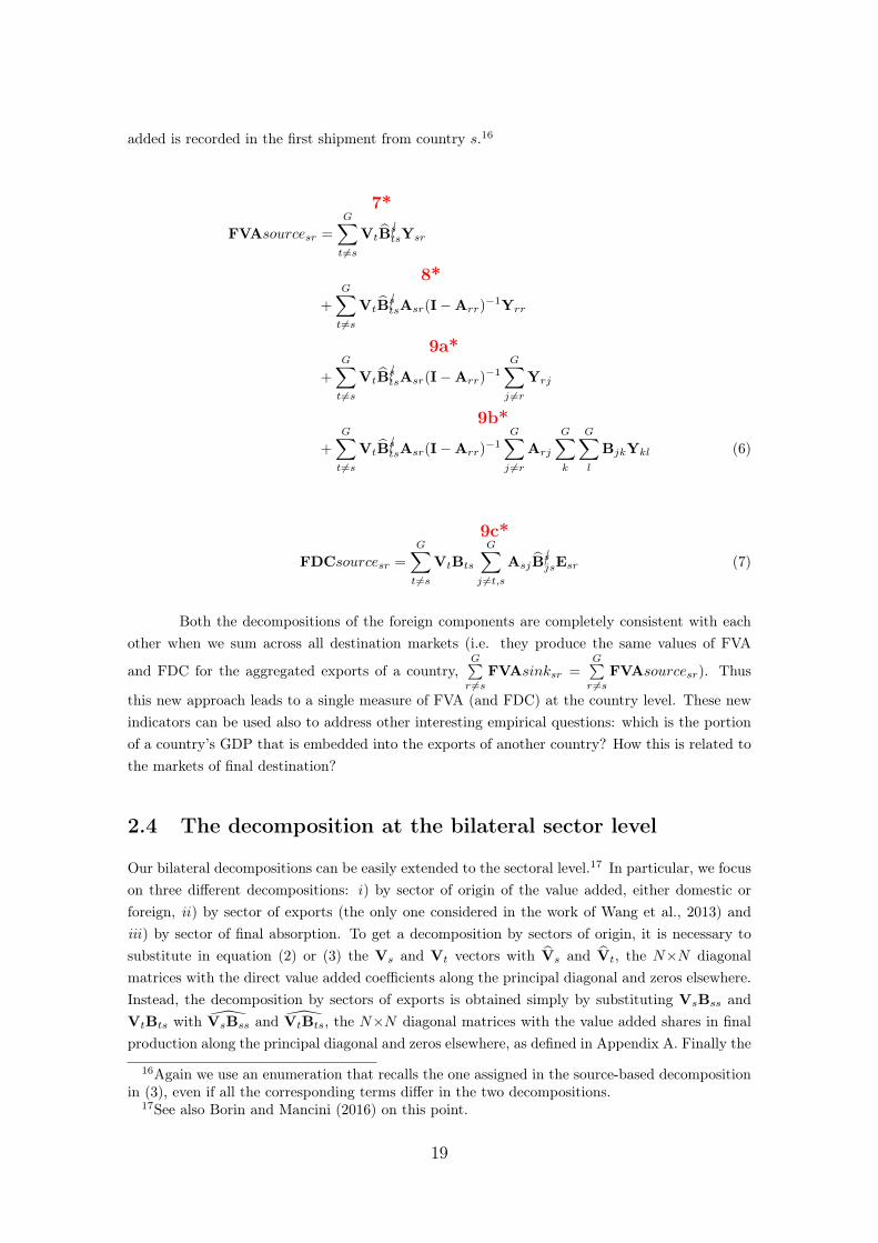
added is recorded in the first shipment from country s.16

FVAsourcesr =

7*G∑

t 6=s

VtB✄stsYsr

+

8*G∑

t 6=s

VtB✄stsAsr(I−Arr)

−1Yrr

+

9a*G∑

t 6=s

VtB✄stsAsr(I−Arr)

−1G∑

j 6=r

Yrj

+

9b*G∑

t 6=s

VtB✄stsAsr(I−Arr)

−1G∑

j 6=r

Arj

G∑

k

G∑

l

BjkYkl (6)

FDCsourcesr =

9c*G∑

t 6=s

VtBts

G∑

j 6=t,s

AsjB✄sjsEsr (7)

Both the decompositions of the foreign components are completely consistent with each

other when we sum across all destination markets (i.e. they produce the same values of FVA

and FDC for the aggregated exports of a country,G∑

r 6=s

FVAsinksr =G∑

r 6=s

FVAsourcesr). Thus

this new approach leads to a single measure of FVA (and FDC) at the country level. These new

indicators can be used also to address other interesting empirical questions: which is the portion

of a country’s GDP that is embedded into the exports of another country? How this is related to

the markets of final destination?

2.4 The decomposition at the bilateral sector level

Our bilateral decompositions can be easily extended to the sectoral level.17 In particular, we focus

on three different decompositions: i) by sector of origin of the value added, either domestic or

foreign, ii) by sector of exports (the only one considered in the work of Wang et al., 2013) and

iii) by sector of final absorption. To get a decomposition by sectors of origin, it is necessary to

substitute in equation (2) or (3) the Vs and Vt vectors with Vs and Vt, the N×N diagonal

matrices with the direct value added coefficients along the principal diagonal and zeros elsewhere.

Instead, the decomposition by sectors of exports is obtained simply by substituting VsBss and

VtBts with VsBss and VtBts, the N×N diagonal matrices with the value added shares in final

production along the principal diagonal and zeros elsewhere, as defined in Appendix A. Finally the

16Again we use an enumeration that recalls the one assigned in the source-based decompositionin (3), even if all the corresponding terms differ in the two decompositions.

17See also Borin and Mancini (2016) on this point.

19

decomposition by sectors of final absorption is obtained by replacing the vectors of final demand,

for instance for country a and b, Yab, with Yab, the N×N diagonal matrices with country’s b de-

mand for final goods produced in a along the principal diagonal and zeros elsewhere.18 Therefore,

depending on the particular empirical application, it will be possible to choose the appropriate

bilateral sectoral decomposition. These decompositions can also be combined: in order to measure

simultaneously the value added embedded in a bilateral trade flow in a particular sector of origin

destined for a particular sector of absorption, it is sufficient to use at the same time V and Y in

equation (2) or (3).

3 Two empirical applications

We use the OECD Trade in Value Added ICIO Tables (TiVA-ICIO, see OECD-WTO, 2012) and

the World Input-Output Database (WIOD, see Dietzenbacher et al. 2013, Timmer et al. 2015)

to show two different ways of exploiting the value added decompositions of bilateral trade. The

first application follows the sink-based approach and focuses on the eight largest world exports,

tracing their domestic VA in exports from direct importers to final demand. The second follows

the source-based approach and derives a new measure of the share of GVC-related trade in order

to determine how its evolution since the mid-1990s has affected the long-run relationship between

global demand and world trade. Matlab codes for the sink and source-based decompositions are

available upon request, both for WIOD and TiVA, as well as those to reproduce the empirical

applications in the next sessions. A Stata command implementing the methods described in

this paper is also available. It can be installed from within Stata by typing net install icio,

from(http://www.econometrics.it/stata).19

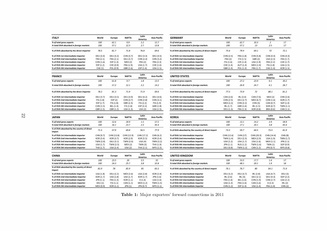
3.1 Major exporters’ forward connections

The decomposition of bilateral export flows provides useful information on the downstream struc-

ture of the production networks in which a country is involved. In particular, in this section

we investigate the channels through which the world top exporters reach the markets of final

destination. We split the domestic value added in exports (DVA) into a share that is directly

exported to the country of ultimate absorption and a share of DVA that passes through one or

more intermediate countries before reaching the final markets. For each exporter and region of

final destination we identify the five most important intermediate importers.

Thus, for this exercise, the sink-based decomposition presented in equation (2) is better

suited, since it accounts the value added the very last time it crosses the national borders, which

is the export flow more closely related with the market of ultimate absorption.20 The exercise is

18See Appendix A for the derivation of V and Y. The matrix VB is obtained in the same way.19Notice that the command cannot be downloaded from the website but just directly installed

through the Stata software.20To further clarify this point we refer to the example shown in Figure 2. With the sink-based

approach all the value added generated in A and finally absorbed in C is entirely accounted withinthe bilateral exports of final goods from A to C, while with the source-based approach a part ofthis would be assigned to the bilateral flow from A to B. See section 2.2 for further details on this

20

carried on with TiVA data for 2011.

We consider the eight largest global exporters (China, US, Germany, Japan, UK, France,

Italy and Korea) and four main regions of destination (Europe, NAFTA, Latin America and

Asia-Pacific), in addition to the world total. First, for each exporter we measure the relative

weight of different markets as ultimate destinations of domestic VA, as compared to their relative

shares in terms of gross exports. Table 1 shows that the two distributions are very similar to

each other only for the US and China. Regarding the Euro Area, Asia-Pacific is a much more

relevant destination in terms of value added compared to gross exports, while the opposite holds

for exports among European countries, since a relevant share of trade flows within the so called

Factory Europe (Baldwin and Lopez-Gonzales, 2013) is made of intermediate goods that cross

many times national borders. Japan and Korea show the most significant divergence between the

gross and the value added composition of exports. In particular, the share of value added exports

towards Asia-Pacific is 10 percentage points lower than the one computed in gross terms.

Then, for each country of exports and region of destination, we single out 1) the share of

domestic VA that is directly absorbed by the bilateral importer, that by definition also belongs to

the region of destination, and 2) the share of domestic VA that passes through one or more inter-

mediate countries (within or outside the region of destination) before reaching the final market.

Regarding the latter, we also identify which are the first five intermediate countries that directly

import from the country of origin.

China’s role as a final hub within the Factory Asia is confirmed looking at Japanese and

Korean exports. Around 20% (17%) of the domestic VA produced in Korea and finally absorbed in

North America (Europe) is embedded in Korean bilateral exports to China. In the case of Japan

the share of domestic VA embedded in exports to China is particularly high for products destined

for the Latin-American market (more than 17% of the total). Also a relevant share of Japanese

and Korean value added that is consumed in the Asia-Pacific region passes through China.

To some extent, a similar role is played by Germany within Factory Europe. Germany

delivers a relevant share of “made in Italy” and “made in France” especially toward more distant

markets: around 4.5% of Italian and French value added destined to the Asia-Pacific market

reaches that region passing through Germany.

China is not only the hub of Factory Asia, but also of the overall global production. In

fact, despite the geographical distance, China is the first intermediate importers for Germany, the

second for the US, the third for Italy and the fourth for France. In particular, it turns out that a

relevant share of European productions destined for the North-American market passes through

China.

point.

21

ITALY World Europe NAFTALatin 

AmericaAsia Pacific GERMANY World Europe NAFTA

Latin America

Asia Pacific

% of total gross exports 100 62.1 9.9 2.2 12.7 % of total gross exports 100 62.7 10.3 2 17

% total DVA absorbed in foreign markets 100 57.1 12.3 2.7 13.8 % total DVA absorbed in foreign markets 100 57.1 13 2.5 17

% of DVA absorbed by the direct importer 78.5 81.7 71.8 76.8 69.6 % of DVA absorbed by the country of direct import 75.6 79.4 69.1 72 72.1

% of DVA 1st intermediate importer DEU (3.4) DEU (3.2) CHN (3.7) DEU (3.3) DEU (4.5) % of DVA 1st intermediate importer CHN (2.5) FRA (1.8) CHN (5.8) CHN (4.4) CHN (4.3)% of DVA 2nd intermediate importer FRA (2.1) FRA (2.1) DEU (3.7) CHN (2.4) CHN (3.2) % of DVA 2nd intermediate importer FRA (2) ITA (1.5) GBR (2) USA (2.3) FRA (1.7)% of DVA 3rd intermediate importer CHN (1.6) ESP (1.3) MEX (2) FRA (2) FRA (2.3) % of DVA 3rd intermediate importer ITA (1.6) CZE (1.4) USA (1.9) FRA (2.2) CHE (1.7)% of DVA 4th intermediate importer ESP (1.2) CHE (0.9) FRA (1.9) USA (1.7) CHE (1.6) % of DVA 4th intermediate importer CHE (1.4) AUT (1.4) MEX (1.9) ITA (1.8) USA (1.5)% of DVA 5th intermediate importer CHE (1) POL (0.9) GBR (1.6) ESP (1.4) USA (1.5) % of DVA 5th intermediate importer GBR (1.4) POL (1.3) FRA (1.7) CHE (1.4) KOR (1.5)

FRANCE World Europe NAFTALatin 

AmericaAsia Pacific UNITED STATES World Europe NAFTA

Latin America

Asia Pacific

% of total gross exports 100 61.8 9.7 1.8 13.5 % of total gross exports 100 27.2 23.9 6.1 30.2

% total DVA absorbed in foreign markets 100 57.2 12.1 2.2 14.2 % total DVA absorbed in foreign markets 100 26.9 24.7 6.1 28.7

% of DVA absorbed by the direct importer 78.2 81.3 71.9 71.9 69.6 % of DVA absorbed by the country of direct import 77.5 73.9 72 88.1 81.2

% of DVA 1st intermediate importer DEU (3.7) DEU (3.5) DEU (3.9) DEU (4.2) DEU (4.6) % of DVA 1st intermediate importer CAN (2.6) IRL (3.4) CAN (7.6) MEX (2) CHN (2.6)% of DVA 2nd intermediate importer ITA (1.8) ESP (2) CHN (3.7) CHN (2.8) CHN (3.1) % of DVA 2nd intermediate importer CHN (2.5) DEU (2.7) MEX (6.7) CHN (1.6) KOR (1.7)% of DVA 3rd intermediate importer ESP (1.7) ITA (1.8) GBR (2.3) ITA (2.2) ITA (1.9) % of DVA 3rd intermediate importer MEX (2.2) CHN (2.2) CHN (3) CAN (0.7) SGP (1.4)% of DVA 4th intermediate importer CHN (1.5) BEL (1.4) ITA (1.8) ESP (2.2) GBR (1.8) % of DVA 4th intermediate importer IRL (1.7) GBR (1.6) IRL (1.5) KOR (0.7) TWN (1.1)% of DVA 5th intermediate importer GBR (1.5) GBR (1.2) USA (1.3) USA (2) USA (1.5) % of DVA 5th intermediate importer DEU (1.3) FRA (1.3) KOR (0.8) BRA (0.6) CAN (1.1)

JAPAN World Europe NAFTALatin 

AmericaAsia Pacific KOREA World Europe NAFTA

Latin America

Asia Pacific

% of total gross exports 100 12.6 18.9 1.5 57.5 % of total gross exports 100 13.1 14.2 2.9 58.9

% total DVA absorbed in foreign markets 100 16.1 23.7 2.5 45.4 % total DVA absorbed in foreign markets 100 17.1 20.1 3.8 45.4

% of DVA absorbed by the country of direct import

71.5 57.9 69.8 56.5 77.9 % of DVA absorbed by the country of direct import 73.5 59.7 64.5 73.5 81.9

% of DVA 1st intermediate importer CHN (9.7) CHN (13.8) CHN (12.9) CHN (17.2) CHN (6.2) % of DVA 1st intermediate importer CHN (12.6) CHN (17) CHN (20.3) CHN (14.4) CHN (8)% of DVA 2nd intermediate importer KOR (3.4) KOR (3.7) KOR (2.9) KOR (5.5) KOR (3.4) % of DVA 2nd intermediate importer TWN (1.4) DEU (2.3) MEX (2.9) USA (1.9) TWN (1.7)% of DVA 3rd intermediate importer TWN (2.8) DEU (3.1) TWN (2.6) USA (4) TWN (3.2) % of DVA 3rd intermediate importer USA (1.2) USA (1.7) USA (1.6) MEX (1.1) JPN (1.1)% of DVA 4th intermediate importer USA (1.7) TWN (2.5) MEX (2) TWN (3) THA (1.9) % of DVA 4th intermediate importer JPN (1.1) RUS (1.2) TWN (1.6) TWN (1) SGP (0.9)% of DVA 5th intermediate importer THA (1.7) USA (2.4) USA (2) THA (2.1) MYS (1.5) % of DVA 5th intermediate importer DEU (0.8) TWN (1.2) CAN (1.2) JPN (0.7) MYS (0.8)

CHINA World Europe NAFTALatin 

AmericaAsia Pacific UNITED KINGDOM World Europe NAFTA

Latin America

Asia Pacific

% of total gross exports 100 23.5 26 3.5 35 % of total gross exports 100 53.5 17.7 1.4 17

% total DVA absorbed in foreign markets 100 24.3 25.7 3.8 32.8 % total DVA absorbed in foreign markets 100 48.1 20.1 1.9 18

% of DVA absorbed by the country of direct import

82.9 78 85.9 85 83.3 % of DVA absorbed by the country of direct import 76.1 76.7 80 64.1 71.9

% of DVA 1st intermediate importer USA (1.8) DEU (2.2) MEX (2.6) USA (2.8) KOR (2.4) % of DVA 1st intermediate importer DEU (3.2) DEU (3.7) IRL (2.8) USA (4.7) DEU (3)% of DVA 2nd intermediate importer KOR (1.7) USA (1.8) USA (1.7) KOR (1.7) JPN (1.6) % of DVA 2nd intermediate importer IRL (2.6) IRL (3) DEU (2.1) DEU (4.3) SGP (2.2)% of DVA 3rd intermediate importer JPN (1.1) FRA (1.3) KOR (1.1) 0 (1.4) USA (1.6) % of DVA 3rd intermediate importer FRA (1.4) BEL (1.6) CHN (1.9) CHN (2.7) USA (2.2)% of DVA 4th intermediate importer DEU (1) ITA (1.1) CAN (1.1) MEX (1.2) TWN (1.5) % of DVA 4th intermediate importer USA (1.3) FRA (1.6) CAN (1.6) 0 (2.3) IRL (2)% of DVA 5th intermediate importer MEX (0.9) KOR (1.1) JPN (1) JPN (0.7) MYS (1.1) % of DVA 5th intermediate importer CHN (1.2) ESP (1.4) USA (1.4) FRA (1.9) CHN (2)

Table 1: Major exporters’ forward connections in 2011

22

3.2 Measuring the weight of Global Value Chains in world

trade

Following the seminal article of Hummels et al. (2001), a number of works have used input-output

tables to gauge the relevance of GVCs in world trade (Johnson and Noguera, 2012; Rahman and

Zhao, 2013; Los et al., 2014). Various measures of the integration of a country (or a region) in

international production networks have been developed. One of the most common is the ‘vertical

specialization’ indicator of Hummels et al. (2001), based on the content of foreign inputs in a

country’s exports. As Cappariello and Felettigh (2014) observe, however, this is only a partial

measure of participation in global value chains, as it considers only the backward linkages. To

take forward linkages too into account, Rahman and Zhao (2013), based on Koopman et al.

(2011), include in the share of trade generated by international fragmentation of production the

domestic value added embedded in the intermediate exports absorbed by third countries and

by the exporting country itself via re-imports. Cappariello and Felettigh (2014) take a similar

approach, measuring the ‘international fragmentation of production’ of a country as the share of

total exports consisting in components 3 to 9 in KWW’s breakdown. The idea is that all trade

flows are related in some way to international production networks, except for the domestic VA

that is directly absorbed by the first importer (1+2 in KWW’s classification).

As we have seen, however, KWW do not properly allocate the domestic VA embedded

in intermediate exports between the share going to direct importers and that absorbed in third

markets. Through the decomposition of bilateral exports we provide a more precise definition of

‘direct absorption’. In particular the source-based methodology is the best suited to this end.

The aim is to single out the trade flows involved in global value chains, conventionally defined as

production processes that require at least two international shipments of goods (including both

intermediate inputs and final products). It is therefore necessary to exclude from GVC-related

trade flows only the fraction of domestic value added that never leaves the first importing country.

In fact this breakdown of bilateral trade flows permits us to single out the fraction of domestic

value added that is exported just once by the domestic country and is directly absorbed by the

importer (terms 1a* and 2a* in equation 3).21 Summing across the bilateral flows, we obtain

the entire domestic value added of country s absorbed by its direct importers without any further

processing abroad or at home, a measure of traditional ‘Ricardian’ trade, as

DAV AXs =

[∑

r 6=s1a*

Vs(I−Ass)−1

G∑

r 6=s

Ysr

+

∑r 6=s

2a*

Vs(I−Ass)−1

G∑

r 6=s

Asr(I−Arr)−1

Yrr

]. (8)

Differently from the sink-based methodology (terms 1 and 2a in equation 2), here the domestic

component of the global inverse Leontief matrix (i.e. Bss) is replaced with the local inverse Leontief

matrix (i.e. (I−Ass)−1). This allows to exclude all the backward linkages of the domestic country

21The notion of ‘direct absorption’ based on a source-based decomposition is slightly differentfrom that considered in the sink-based one, employed in the empirical application of section 3.1.Since the sink-based classification aims to map value added accordingly to the ultimate destinationmarket, the ‘direct absorption’ term also include the domestic VA absorbed by direct bilateralimporters after additional processing abroad, i.e. 2b and 3c in equation (2).

23

within the international production networks.22

Thus, it is possible to measure GVC-related trade flows simply by excluding the entire

domestic value added of country s absorbed directly by his direct importers (DAV AXs) from his

total exports:

GV CXs = uNEs∗ −DAV AXs. (9)

Therefore, GVC-related trade share in total exports is

GV Cs =GV CXs

Es∗

, (10)

where Es∗ = uNEs∗.

Employing WIOD tables, we have computed the share of GVC-related trade in total

world exports using three different methods (see Table 2): an index of vertical specialization very

similar to one proposed by Hummels et al. (2001); a GVC indicator based on components 3 to

9 of the original KWW decomposition (GVC-KWW), as calculated in Cappariello and Felettigh

(2015); and our own GVC measure in equation (10). In the last column we also computed our

own measure of GVC employing OECD-TiVA tables. Our indicator puts the share of GVC-related

trade at between a third and nearly half the total during our sample period and it does not change

much whether it is computed with WIOD or OECD-TiVA tables.23 As expected, our indicator

finds a considerably larger weight of GVCs in total trade than the KWW decomposition, which in

turn gives a share about 10 percentage points greater than the fraction indicated by the vertical

specialization indicator. Almost all of the difference between our indicator and the measure

derived from the original KWW decomposition is due to the different classification of the value

added absorbed by direct importers, whereas the impact of using the local as against the global-

domestic Leontief is minor. Nevertheless, the evolution of the three indicators over time is quite

similar.

There are at least two factors that could bias these measures of international fragmenta-

tion. First, changes in commodity prices. Commodity cycles may inflate or deflate nominal trade

statistics. In particular, total trade and GVC trade could be affected asymmetrically by commod-

ity price fluctuations. Therefore GVC participation indices could be biased. Furthermore, it is

not clear whether commodity trade should be included in the notion of GVC trade. Import of raw

materials falls within the concept of trade induced by differences in resource and factor endow-

22To grasp the difference between these two measures, consider the following example. Supposethat country A performs the first stage of a production process, ships the intermediate productsabroad for a second processing stage, and re-imports them for final completion. Finally, the goodsare exported to serve final demand. Computing the domestic value added embedded in the exportsof final goods using the local inverse Leontief matrix ((I−AAA)

−1 we consider only the last stageof production performed in A, while with the sub-componet BAA of the global Leontief matrixwe take account of the VA generated both in the first and in the last stage. Thus the Bss matrixdiffers from the local Leontief whenever two (or more) distinct stages of production are performedin the domestic country s. Since this entails some international fragmentation of production, itwould appear better, in computing the portion of trade that is not involved in GVC, to use thelocal Leontief matrix.

23The weight of GVC-related trade might seem quite great, and to be sure there are some factorsthat could result in an overestimate of this and other measures of GVC-related trade. For example,the separate consideration of each country in the highly integrated euro area could engender anupward bias (Amador et al., 2015)

24

VS GVC-KWW GVC GVC (TiVA)share ∆ share ∆ share ∆ share ∆

1995 18.8 27.9 34.7 33.2

2000 22.1 3.3 32.7 4.8 40.0 5.3 39.1 6.0

2005 24.4 2.2 35.0 2.3 43.5 3.4 41.2 2.1

2011 26.2 1.8 36.0 1.0 44.7 1.2 43.7 2.5

Table 2: Indices of international fragmentation. Columns 1-3 are based on WIOD data,

column 4 on OECD TiVA.

VS : vertical specialization, foreign value added and both domestic and foreign double count-ing on total exports; GVC-KWW : index of international fragmentation used in Capparielloand Felettigh (2015), summing terms 3 to 9 of KWW decomposition, on total exports; GVC

refined index calculated as total exports excluding terms 1a* and 2a* of our source-baseddecomposition, on total exports. All indices are computed excluding exports from the “Restof the world”.

ments, while the common notion of GVC-related trade has to do with the international shipments

of parts and components at a more advanced stage of production. In order to exclude trade in

commodities without affecting the entire international production structure we modify the original

input-output table setting the value added produced in the energy sectors24 to zero.25 It turns

out that the commodity cycle has inflated the GVC measure of trade in the period 2003-2008.26

Second, changes in demand composition. In principle, the relevance of global value chains

and their evolution over time should be evaluated on the basis of the international production

structure, i.e. from a supply side perspective. However, given that final goods and services differ in

terms of their GVC intensity in production, any change in demand composition will affect also the

aggregate measures of GVC-related trade. Think for instance at business cycle fluctuations, where

some final demand components, such as capital goods, are at the same time more procyclical and

GVC-intensive than others. Then we adjust our indicators of GVC-related trade by “neutralizing”

the changes in demand composition, and using constant prices input-output tables available in

the WIOD database.27

24Mining and Quarrying and Coke, Refined Petroleum and Nuclear Fuel.25Following this strategy, a brand new input-output table, a vector of gross output and a matrix

of final demand are computed. It is worth noting that energy sectors still operate, but they justbounce intermediate goods that are destined to them, without adding value. Without this artifice,simply shutting down those sectors, also value added originated in other sectors would have beencanceled out.

26The difference between the GVC-related trade index computed using adjusted data withrespect to the original one starts to expand from 2003, when commodity prices begin their rise.The wedge follows closely the commodity price index movements. The correlation between thetwo series is 0.99.

27The procedure to reach this goal is the following. First of all, the final demand at time t-1is used to replace the final demand at time t in order to calculate a new gross output vector attime t (and prices t-1 ) fully coherent with the demand at t-1. In this way we are able to computea GVC index with demand and prices at t-1 but with the international production structure oftime t. Then it is possible to compute year on year variations of the GVC index net of changes indemand and prices. Finally we obtain the full time series chaining these variations starting fromthe 1995 GVC level.

25

As is shown by the red line in Figure 6, the GVC share of total trade, measured as in

equation (10), has been growing since the mid-1990s, reaching 40% in 2004. In 2009, during the

crisis, the unadjusted GVC share on total trade (yellow bar) contracted dramatically, by about

5 percentage points. However, almost half of this drop is accounted for equally by changes in

demand composition and in commodity prices. Therefore it is crucial to control for these two

factors in assessing the diffusion of international fragmentation and its evolution over time.28

After the crisis, GVC share has recovered only marginally.

‐6

‐5

‐4

‐3

‐2

‐1

0

1

2

3

4

0

5

10

15

20

25

30

35

40

45

50

1995 1997 1999 2001 2003 2005 2007 2009 2011

GVC share changes (commodity price and demand adjusted)

GVC share changes (commodity price adjusted)

GVC share changes (no adjustment)

GVC share on total trade (commodity price and demand adjusted, LHS)

Figure 5: GVC share, level and growth rates

These measures of international fragmentation can be employed to quantify the contribu-

tion of global value chains in explaining the decline of the income elasticity of trade, i.e. the ratio

of trade to GDP growth. In fact, while cyclical factors - the investment slump, the weakness of

economic activity in the euro area - have been key drivers of the trade slowdown, a major role

has also been played by structural factors, including global value chains, as suggested by Con-

stantinescu et al. (2015), Ferrantino and Taglioni (2014) and Escaith et al. (2010). Since world

exports are equal to world imports (i.e. at any time t we have that M(t) = E(t) =∑G

s Es∗), we

can express the latter as the sum of traditional ‘Ricardian’ trade (DAV AX(t)) plus GVC-related

trade (GV CX(t)). We define world imports as

M(t) ≡M(t)

DAV AX(t)

DAV AX(t)

Y(t)Y(t). (11)

28The relevance of the correction is clear also in 2008, when the increase in commodity pricehas inflated the change in the GVC-trade share by almost 1 percentage point. In general theunadjusted measure is more volatile than the adjusted one, leading to an incorrect picture of theglobal value chain diffusion.

26

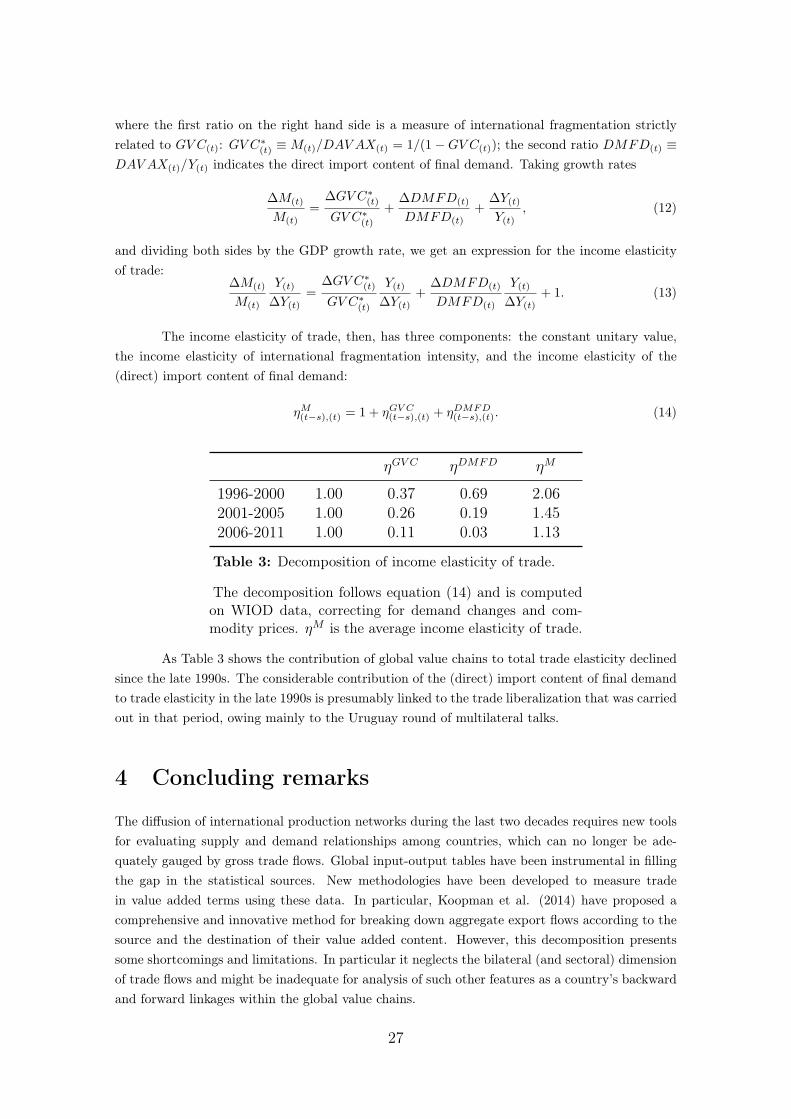
where the first ratio on the right hand side is a measure of international fragmentation strictly

related to GV C(t): GV C∗(t) ≡ M(t)/DAV AX(t) = 1/(1−GV C(t)); the second ratio DMFD(t) ≡

DAV AX(t)/Y(t) indicates the direct import content of final demand. Taking growth rates

∆M(t)

M(t)=

∆GV C∗(t)

GV C∗(t)

+∆DMFD(t)

DMFD(t)+

∆Y(t)

Y(t), (12)

and dividing both sides by the GDP growth rate, we get an expression for the income elasticity

of trade:∆M(t)

M(t)

Y(t)

∆Y(t)=

∆GV C∗(t)

GV C∗(t)

Y(t)

∆Y(t)+

∆DMFD(t)

DMFD(t)

Y(t)

∆Y(t)+ 1. (13)

The income elasticity of trade, then, has three components: the constant unitary value,

the income elasticity of international fragmentation intensity, and the income elasticity of the

(direct) import content of final demand:

ηM(t−s),(t) = 1 + ηGV C(t−s),(t) + ηDMFD

(t−s),(t). (14)

ηGV C

ηDMFD

ηM

1996-2000 1.00 0.37 0.69 2.06

2001-2005 1.00 0.26 0.19 1.45

2006-2011 1.00 0.11 0.03 1.13

Table 3: Decomposition of income elasticity of trade.

The decomposition follows equation (14) and is computedon WIOD data, correcting for demand changes and com-modity prices. ηM is the average income elasticity of trade.

As Table 3 shows the contribution of global value chains to total trade elasticity declined

since the late 1990s. The considerable contribution of the (direct) import content of final demand

to trade elasticity in the late 1990s is presumably linked to the trade liberalization that was carried

out in that period, owing mainly to the Uruguay round of multilateral talks.

4 Concluding remarks

The diffusion of international production networks during the last two decades requires new tools

for evaluating supply and demand relationships among countries, which can no longer be ade-

quately gauged by gross trade flows. Global input-output tables have been instrumental in filling

the gap in the statistical sources. New methodologies have been developed to measure trade

in value added terms using these data. In particular, Koopman et al. (2014) have proposed a

comprehensive and innovative method for breaking down aggregate export flows according to the

source and the destination of their value added content. However, this decomposition presents

some shortcomings and limitations. In particular it neglects the bilateral (and sectoral) dimension

of trade flows and might be inadequate for analysis of such other features as a country’s backward

and forward linkages within the global value chains.

27

We propose two decompositions of bilateral exports that are largely consistent with the

KWW approach. In line with the spirit of Nagengast and Stehrer (2016), a first one takes the

perspective of the country where the value added originates (the source-based approach), a second

one that of the country that ultimately absorbs it in final demand (the sink-based approach). This

allows to choose the most appropriate approach to the purpose of the analysis.

The original components in KWW can be retrieved from our decompositions by summing

the bilateral export flows across the destinations. At the same time, we also refine the classification

of domestic and foreign value added embedded in exports, correcting some inexactnesses of KWW’s

methodology. In particular, our approach can both account for the entire domestic value added

embedded in bilateral shipments and discriminate precisely between the exports that are finally

absorbed by the direct importers and those that are consumed in third countries. These issues

have not been properly addressed by KWW or in the rest of the literature (see Wang et al.,

2013; Nagengast and Stehrer, 2016). Moreover, this allows us to derive for the first time a precise

measure of GVC-related trade in the spirit of the definition proposed by Hummels et al. (2001).

We also correct the KWW measures of foreign value added and foreign double counted; the refined

measures turn out to be consistent with those proposed by Johnson (2017) when computed for

world trade flows.

We also develop further the accounting of the foreign content of exports providing brand

new definitions that take the perspective of the exporting country. Following the same logic of the

domestic content of exports we define as foreign double counted only the items that cross the same

(national) borders more than once. Both the new bilateral sink-based breakdown of the foreign

content of exports and the source-based one produce the same indicators of FVA and FVC at the

country level.

Finally, our bilateral decompositions can be easily extended to take into account the

sectoral dimension. We consider three different perspectives: i) the sector of origin of the value

added, either domestic or foreign, ii) the sector of exports and iii) the sector of final absorption.

Examining bilateral flows through the lens of their value added content, we can for example

assess a country’s position within the international production processes, identifying the direct

upstream and downstream trade partners. In this way we can also gauge the effect on bilateral

trade balances exerted by participation in GVCs and by final demand from third countries.

With our sink-based decomposition we investigate the channels through which the world

top exporters reach the markets of final destination. The results of the analysis confirm the role

of China as a final assembly hub, in particular within the Factory Asia, but also in other relevant

inter-regional production networks. As a matter of fact most of the value added produced in China

is shipped directly to the market of final demand, while a non-negligible share of other countries’

exports to China are ultimately destined to third countries. To some extent, Germany plays a

similar role, but mainly for countries that take part in Factory Europe.

In a second, separate, empirical application we use our source-based bilateral decompo-

sition to compute our new measure of international fragmentation of production. The share of

GVC-related trade in total trade has been growing since mid-1990s, reaching 43.5% in 2005. In

2009 this index shrank dramatically and in the aftermath of the recession it has recovered only

marginally. However, there are at least two factors that could distort this measure of international

28

fragmentation, changes in commodity prices and in demand composition. Indeed once we adjust

the indicator of GVC-related trade for these factors half of the drop recorded in 2009 disappears.

Nevertheless, even applying this correction, we still do not find a strong rebound of GVC-trade

after the crisis. This could be also one of the causes of the weakness of global trade in most recent

years. In order to shed more light on this point, our measure of GVC-related trade has been used

to inquire into the role played by international fragmentation of production in the changes of the

long-term relation between trade and income. We find that the contribution of GVC diffusion to

the income elasticity of trade has been steadily declining since the late 1990s.

Besides the examples provided here, the proposed breakdown of bilateral/sectoral gross

exports also produces the basic information needed to address several issues related to global

production networks, such as country/sector position and participation in GVCs. In this way it

will be possible to investigate at the macro (country-sector) level some of the features of GVCs

that insofar have been mainly examined in case studies or in firm level analyses.

References

Amador, J., R. Cappariello, and R. Stehrer, 2015. ‘Global Value Chains: A View from the Euro

Area’. ECB Working Paper Series, No 1761.

Antràs, P. and D. Chor, 2013. ‘Organizing the global value chain.’ Econometrica, 2013, 81(6),

pp. 2127-2204.

Baldwin, R. and J. Lopez-Gonzalez, 2013. ‘Supply-Chain Trade: A Portrait of Global Patterns

and Several Testable Hypotheses.’, NBER Working Paper, No. 18957.

Borin, A. and M. Mancini, 2016. ‘Participation in Global Value Chains: Measurement Issues and

the Place of Italy’, Rivista di Politica Economica.

Brancati, E., R. Brancati and A. Maresca, 2017. ‘Global value chains, innovation and performance:

firm-level evidence from the Great Recession’, Journal of Economic Geography.

Cappariello, R. and A. Felettigh, 2015. ‘How does foreign demand activate domestic value added?

A comparison among the largest euro-area economies.’ Temi di Discussione (Working Papers)

1001, Bank of Italy.

Constantinescu, C., A. Mattoo and M. Ruta, 2015, ‘The global trade slowdown: cyclical or struc-

tural?’ IMF Working Paper 15/6.

Daudin, G., C. Rifflart and D. Schweisguth, 2009. ‘Who produces for whom in the world economy?’

Document de travail de l’OFCE N◦ 2009-18, July.

Dedrick, J., K. L. Kraemer, and G. Linden, 2010. ‘Who profits from innovation in global value

chains?: a study of the iPod and notebook PCs.’ Industrial and corporate change, 19.1 pp. 81-116.

Dietzenbacher, E., B. Los, R. Stehrer, M.P. Timmer and G.J. de Vries, 2013. ‘The Construction

of World Input-Output Tables in the WIOD Project.’ Economic Systems Research, 25, pp. 71-98.

Escaith, H, N. Lindenberg and S. Miroudot, 2010. ‘International Supply Chains and Trade Elas-

ticity in Times of Global Crisis.’ MPRA Paper 20478, University Library of Munich, Germany.

29

Ferrantino, M. J., and D. Taglioni, 2014. ‘Global value chains in the current trade slowdown.’

World Bank-Economic Premise 138 (2014): 1-6.

Hummels, D., J. Ishii and K.M. Yi, 2001. ‘The Nature and Growth of Vertical Specialization in

World Trade.’ Journal of International Economics, 54, pp. 75-96.

Ivarsson, I., and C. G. Alvstam, 2011. ‘Upgrading in global value-chains: a case study of

technology-learning among IKEA-suppliers in China and Southeast Asia.’ Journal of Economic

Geography, 11 (4), pp. 731-752.

Johnson, R. C., 2017. ‘Measuring Global Value Chains’, Annual Review of Economics, forthcom-

ing.

Johnson, R. C. and G. Noguera, 2012. ‘Accounting for Intermediates: Production Sharing and

Trade in Value Added.’ Journal of International Economics, 86, Iss. 2, pp. 224-236.

Koopman, R., W. Powers, Z. Wang and S. Wei, 2011. ‘Give Credit Where Credit is Due: Tracing

Value-added in Global Production Chains.’ NBER Working Paper, No. 16426.

Koopman, R., Z. Wang and S. Wei, 2014. ‘Tracing Value-Added and Double Counting in Gross

Exports.’ American Economic Review, 104(2): 459-94.

Los, B., M. P. Timmer and G. de Vries, 2014. ‘How Global Are Global Value Chains? A New

Approach to Measure International Fragmentation.’ Journal of Regional Science, 55, No. 1, pp.

66-92.

Nagengast, A.J. and R. Stehrer, 2016. ‘Collateral imbalances in intra-European trade? Accounting

for the differences between gross and value added trade balances’ The World Economy.

OECD-WTO, 2012. ‘Trade in Value Added: concepts, methodologies and challenges’, http:

//www.oecd.org/sti/ind/49894138.pdf.

Rahman, J. and T. Zhao, 2013. ‘Export Performance in Europe : What Do We Know from Supply

Links?’ IMF Working Paper, No. 13/62.

Sturgeon T., J. Van Biesebroeck and G. Gereffi, 2008. ‘Value chains, networks and clusters:

reframing the global automotive industry.’ Journal of Economic Geography, 8 pp. 297-321.

Timmer, M. P., E. Dietzenbacher, B. Los, R. Stehrer and G.J. de Vries, 2015. ‘An Illustrated

User Guide to the World Input-Output Database: the Case of Global Automotive Production.’

Review of International Economics, forthcoming.

Wang, Z., S. Wei, X. Yu and K. Zhu, 2016. ‘Characterizing Global Value Chains.’ mimeo (available

at http://www.cepr.org/sites/default/files/Wang,%20Zhi.pdf).

Wang, Z., S. Wei and K. Zhu, 2013. ‘Quantifying International Production Sharing at the Bilateral

and Sector Levels.’ NBER Working Paper, No. 19677.

30

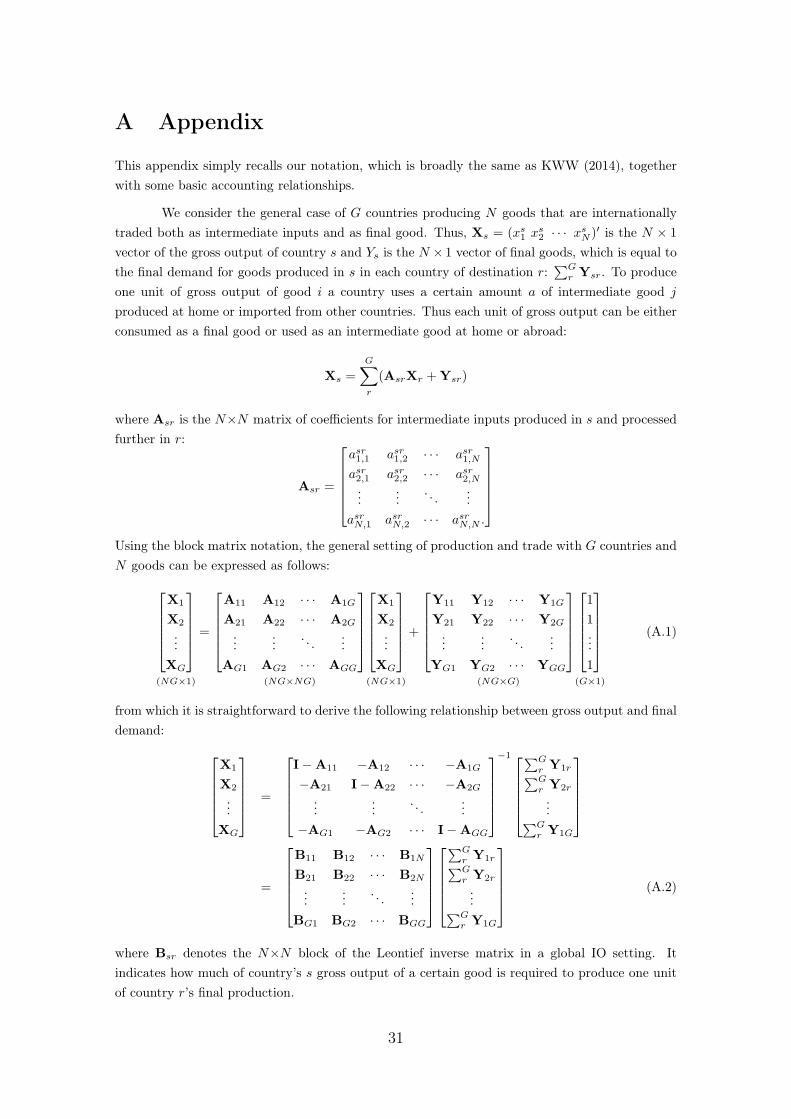
A Appendix

This appendix simply recalls our notation, which is broadly the same as KWW (2014), together

with some basic accounting relationships.

We consider the general case of G countries producing N goods that are internationally

traded both as intermediate inputs and as final good. Thus, Xs = (xs1 xs

2 · · · xsN )′ is the N × 1

vector of the gross output of country s and Ys is the N × 1 vector of final goods, which is equal to

the final demand for goods produced in s in each country of destination r:∑G

r Ysr. To produce

one unit of gross output of good i a country uses a certain amount a of intermediate good j

produced at home or imported from other countries. Thus each unit of gross output can be either

consumed as a final good or used as an intermediate good at home or abroad:

Xs =

G∑

r

(AsrXr +Ysr)

where Asr is the N×N matrix of coefficients for intermediate inputs produced in s and processed

further in r:

Asr =

asr1,1 asr1,2 · · · asr1,Nasr2,1 asr2,2 · · · asr2,N

......

. . ....

asrN,1 asrN,2 · · · asrN,N .

Using the block matrix notation, the general setting of production and trade with G countries and

N goods can be expressed as follows:

X1

X2

...

XG

(NG×1)

=

A11 A12 · · · A1G

A21 A22 · · · A2G

......

. . ....

AG1 AG2 · · · AGG

(NG×NG)

X1

X2

...

XG

(NG×1)

+

Y11 Y12 · · · Y1G

Y21 Y22 · · · Y2G

......

. . ....

YG1 YG2 · · · YGG

(NG×G)

1

1...

1

(G×1)

(A.1)

from which it is straightforward to derive the following relationship between gross output and final

demand:

X1

X2

...

XG

=

I−A11 −A12 · · · −A1G

−A21 I−A22 · · · −A2G

......

. . ....

−AG1 −AG2 · · · I−AGG

−1

∑G

r Y1r∑G

r Y2r

...∑G

r Y1G

=

B11 B12 · · · B1N

B21 B22 · · · B2N

......

. . ....

BG1 BG2 · · · BGG

∑G

r Y1r∑G

r Y2r

...∑G

r Y1G

(A.2)

where Bsr denotes the N×N block of the Leontief inverse matrix in a global IO setting. It

indicates how much of country’s s gross output of a certain good is required to produce one unit

of country r’s final production.

31

It is useful to recall two equivalences that are used extensively in KWW (2014) and that

we use to derive the results presented in section 2. Considering the following property of inverse

matrix B:

B(I−A) = (I−A)B = I

it is easily shown that the generic block diagonal element Bss may be expressed as follows:

Bss =G∑

t 6=s

BstAts(I−Ass)−1 + (I−Ass)

−1 =

= (I−Ass)−1 + (I−Ass)

−1G∑

t 6=s

AstBts (A.3)

while the generic off-diagonal block element Brs corresponds to:

Brs =

G∑

t 6=s

BrtAts(I−Ass)−1 =

= (I−Arr)−1

G∑

t 6=r

ArtBts (A.4)

The direct value added share in each unit of gross output produced by country s is equal to

one minus the sum of the direct intermediate input share of all the domestic and foreign suppliers:

Vs = uN (I−

G∑

r

Ars) (A.5)

where uN is the 1×N unit row vector. Thus the G×GN direct domestic value added matrix for

all countries can be defined as:

V =

V1 0 · · · 0

0 V2 · · · 0

......

. . ....

0 0 · · · VG

while the overall G×GN value added share matrix is obtained by multiplying the V matrix by

the Leontief inverse B:

VB =

V1B11 V1B12 · · · V1B1G

V2B21 V2B22 · · · V2B2G

......

. . ....

VGBG1 VGBG2 · · · VGBGG

Since the domestic value shares of different countries in final demand have to sum to one

the following property holds:G∑

r

VsBsr = uN (A.6)

32

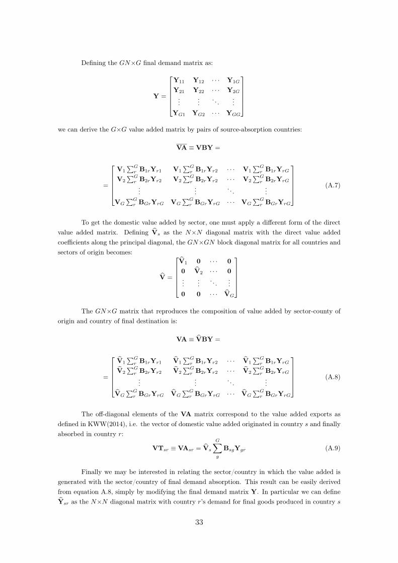
Defining the GN×G final demand matrix as:

Y =

Y11 Y12 · · · Y1G

Y21 Y22 · · · Y2G

......

. . ....

YG1 YG2 · · · YGG

we can derive the G×G value added matrix by pairs of source-absorption countries:

VA ≡ VBY =

=

V1

∑G

r B1rYr1 V1

∑G

r B1rYr2 · · · V1

∑G

r B1rYrG

V2

∑G

r B2rYr2 V2

∑G

r B2rYr2 · · · V2

∑G

r B2rYrG

......

. . ....

VG

∑G

r BGrYrG VG

∑G

r BGrYrG · · · VG

∑G

r BGrYrG

(A.7)

To get the domestic value added by sector, one must apply a different form of the direct

value added matrix. Defining Vs as the N×N diagonal matrix with the direct value added

coefficients along the principal diagonal, the GN×GN block diagonal matrix for all countries and

sectors of origin becomes:

V =

V1 0 · · · 0

0 V2 · · · 0

......

. . ....

0 0 · · · VG

The GN×G matrix that reproduces the composition of value added by sector-county of

origin and country of final destination is:

VA ≡ VBY =

=

V1

∑G

r B1rYr1 V1

∑G

r B1rYr2 · · · V1

∑G

r B1rYrG

V2

∑G

r B2rYr2 V2

∑G

r B2rYr2 · · · V2

∑G

r B2rYrG

......

. . ....

VG

∑G

r BGrYrG VG

∑G

r BGrYrG · · · VG

∑G

r BGrYrG

(A.8)

The off-diagonal elements of the VA matrix correspond to the value added exports as

defined in KWW(2014), i.e. the vector of domestic value added originated in country s and finally

absorbed in country r:

VTsr ≡ VAsr = Vs

G∑

g

BsgYgr (A.9)

Finally we may be interested in relating the sector/country in which the value added is

generated with the sector/country of final demand absorption. This result can be easily derived

from equation A.8, simply by modifying the final demand matrix Y. In particular we can define

Ysr as the N×N diagonal matrix with country r’s demand for final goods produced in country s

33

along the principal diagonal:

Ysr =

ysr1 0 · · · 0

0 ysr2 · · · 0...

.... . .

...

0 0 · · · ysrN

Then the distribution of global value added by combinations of sector/county of origin

and sector-country of final destination is represented by the following GN×GN matrix:

VA ≡ VBY =

=

V1

∑G

r B1rYr1 V1

∑G

r B1rYr2 · · · V1

∑G

r B1rYrG

V2

∑G

r B2rYr2 V2

∑G

r B2rYr2 · · · V2

∑G

r B2rYrG

......

. . ....

VG

∑G

r BGrYrG VG

∑G

r BGrYrG · · · VG

∑G

r BGrYrG

(A.10)

34

B Appendix

The gross bilateral exports of country s to country r consist in final goods and intermediate inputs

for the production of gross output in country r (Xr):

Esr = Ysr +AsrXr. (B.1)

In country r, in turn, the intermediate inputs imported from s undergo one or more processing

phases to produce final products for domestic consumption or goods for re-export (both interme-

diate and final):

AsrXr = Asr(I−Arr)−1

Yrr +Asr(I−Arr)−1

Er∗. (B.1-bis)

Thus bilateral exports can be re-expressed as:

Esr = Ysr +Asr(I−Arr)−1

Yrr +Asr(I−Arr)−1

Er∗ (B.2)

From equation (B.2) we can already identify some of the components of the KWW decomposition

simply by applying the following property of the value added matrix VB (see A.6):

uN = VsBss +

G∑

t 6=s

VtBts

Applying this equivalence to both sides of equation B.2, we get an initial decomposition of bilateral

gross exports in value added terms:

uNEsr = VsBssYsr +VsBssAsr(I−Arr)−1

Yrr

+ VsBssAsr(I−Arr)−1

Er∗

+

G∑

t 6=s

VtBtsYsr +

G∑

t 6=s

VtBtsAsr(I−Arr)−1

Yrr

+

G∑

t 6=s

VtBtsAsr(I−Arr)−1

Er∗ (B.3)

The first term in (B.3) is the counterpart of KWW’s ‘domestic value added in direct

final goods exports’. Indeed, the sum of VsBssYsr across all the r countries of destination gives

exactly the first term in KWW’s decomposition. Since it makes use of (a portion of) the global

inverse Leontief matrix B, this term fully account for the entire domestic value added embedded in

exports of final goods. This means that if a certain product requires a first stage of processing at

home, a second stage abroad and a final stage again at home, the domestic value added generated

in both the first and the last stages is fully accounted for in this term. The peculiar feature of the

sink-based approach is indeed to record the value added originated in all the upstream production

stages the last time that a certain product leaves the country.

The last three terms in (B.3) correspond to the last three items of KWW accounting of

total gross exports. However the last term do not entirely corresponds to the the foreign double

35

counted component in exports, as stated by KWW. To correctly single out all the FVA in exports

we have to split the the last term in (B.3) between the part originally produced in the importing

country r and that produced elsewhere.

G∑

t 6=s

VtBtsAsr(I−Arr)−1

Er∗ =

G∑

t 6=s,r

VtBtsAsr(I−Arr)−1

Er∗

+ VrBrsAsr(I−Arr)−1

Er∗ (B.4)

The first term on the right hand side of equation (B.4) is indeed double counted, while the

part in the last term that correspond to the exports of country r to the market of final destination

is still foreign value added and it can be singled out as follows.

G∑

t 6=s

VtBtsAsr(I−Arr)−1

Er∗ = VrBrsAsr(I−Arr)−1

G∑

j 6=r

Yrj

+ VrBrsAsr(I−Arr)−1

G∑

j 6=r

Arj(I−Ajj)−1

Yjj

+ VrBrsAsr(I−Arr)−1

G∑

j 6=r

Arj(I−Ajj)−1

Ej∗

+

G∑

t 6=s,r

VtBtsAsr(I−Arr)−1

Er∗ (B.5)

where the first two terms on the right hand side of equation (B.5) represent a component of the

foreign value added of exports not considered by KWW.

We now can come back to the decomposition of the domestic component of exports. We

can define the second term in equation (B.3) (VsBssAsr(I−Arr)−1

Yrr) as the actual ‘domestic

value added in intermediate exports absorbed by direct importers’(without any further processing

abroad). However, this item differs from what KWW designate by this expression. Indeed, as

Nagengast and Stehrer (2016) point out, the second term in KWW’s decomposition does not

encompass only the domestic value added exports in the intermediate products directly exported

to country r and then processed to satisfy r’s final demand. Rather, it corresponds to the total

value added generated in s and contained in the goods finally produced and consumed in r,

including products not exported directly to that country.

Now we consider the domestic content of intermediate goods processed in r and then re-

exported to s or to third countries (i.e. the third term in B.3). Recalling the accounting identity

used in B.1, we can split the (re)exports from country r into intermediate goods and final products,

isolating among the latter the re-imports of the original exporter, country s.

Er∗ =G∑

j 6=r,j 6=s

Yrj +Yrs +G∑

j 6=r

ArjXj (B.6)

36

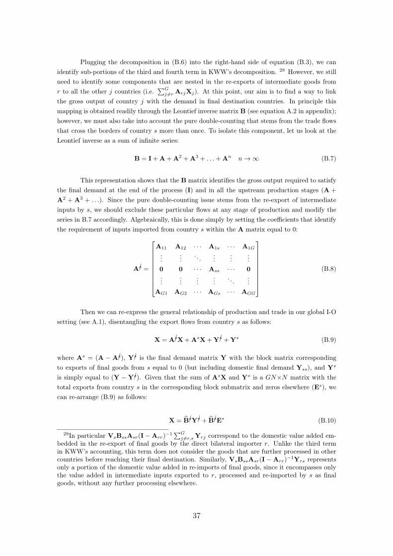
Plugging the decomposition in (B.6) into the right-hand side of equation (B.3), we can

identify sub-portions of the third and fourth term in KWW’s decomposition. 29 However, we still

need to identify some components that are nested in the re-exports of intermediate goods from

r to all the other j countries (i.e.∑G

j 6=r ArjXj). At this point, our aim is to find a way to link

the gross output of country j with the demand in final destination countries. In principle this

mapping is obtained readily through the Leontief inverse matrix B (see equation A.2 in appendix);

however, we must also take into account the pure double-counting that stems from the trade flows

that cross the borders of country s more than once. To isolate this component, let us look at the

Leontief inverse as a sum of infinite series:

B = I+A+A2 +A

3 + . . .+An n → ∞ (B.7)

This representation shows that the B matrix identifies the gross output required to satisfy

the final demand at the end of the process (I) and in all the upstream production stages (A +

A2 + A

3 + . . .). Since the pure double-counting issue stems from the re-export of intermediate

inputs by s, we should exclude these particular flows at any stage of production and modify the

series in B.7 accordingly. Algebraically, this is done simply by setting the coefficients that identify

the requirement of inputs imported from country s within the A matrix equal to 0:

A✄s =

A11 A12 · · · A1s · · · A1G

......

. . ....

......

0 0 · · · Ass · · · 0

......

......

. . ....

AG1 AG2 · · · AGs · · · AGG

(B.8)

Then we can re-express the general relationship of production and trade in our global I-O

setting (see A.1), disentangling the export flows from country s as follows:

X = A✄sX+AsX+Y ✄s +Y

s (B.9)

where As = (A − A✄s), Y ✄s is the final demand matrix Y with the block matrix corresponding

to exports of final goods from s equal to 0 (but including domestic final demand Yss), and Ys

is simply equal to (Y −Y ✄s). Given that the sum of AsX and Y

s is a GN×N matrix with the

total exports from country s in the corresponding block submatrix and zeros elsewhere (Es), we

can re-arrange (B.9) as follows:

X = B✄sY ✄s + B✄sEs (B.10)

29In particular VsBssAsr(I −Arr)−1

∑G

j 6=r,s Yrj correspond to the domestic value added em-bedded in the re-export of final goods by the direct bilateral importer r. Unlike the third termin KWW’s accounting, this term does not consider the goods that are further processed in othercountries before reaching their final destination. Similarly, VsBssAsr(I −Arr)

−1Yrs represents

only a portion of the domestic value added in re-imports of final goods, since it encompasses onlythe value added in intermediate inputs exported to r, processed and re-imported by s as finalgoods, without any further processing elsewhere.

37

where B✄s ≡ (I − A✄s)−1 is the Leontief inverse matrix derived from the new input coefficient

matrix A✄s, which excludes the input requirement of other economies from country s.30 Since

Xj =∑G

l Xjl, we can apply the new accounting relationship in (B.10) to the decomposition of

(re)exports from the original importer r (equation B.6):

Er∗ =

G∑

j 6=r,j 6=s

Yrj +Yrs +

G∑

j 6=r

Arj

G∑

k 6=s

G∑

l

B✄sjkYkl

+G∑

j 6=r

ArjB✄sjsYss +

G∑

j 6=r

ArjB✄sjsEs∗ (B.11)

We can now fully decompose bilateral exports from s to r into the domestic and foreign

value added embedded in final demand (Y) and the pure double counted components. All we

need to do now is further disentangle the third term in equation (B.11) to distinguish: i) the

domestic value added finally absorbed in the country of origin through the imports of final goods

(∑G

k 6=s Yks); ii) the domestic value added finally absorbed in a foreign country as a local good

(∑G

l 6=s Yll); and iii) the domestic value added finally absorbed in a foreign country as a foreign

good (∑G

k 6=s

∑G

l 6=s,k Ykl).

30Notice that the domestic input coefficient matrix Ass is part of the A✄s matrix, in which onlythe other Ast submatrices, with t 6= s, have all the elements equal to zero. This allows to include inthe domestic value added of exports of the goods that undergo a final processing stage in countrys and are ultimately used there.

38

C Appendix

In this Appendix we show that each component of KWW’s original decomposition (equation 36 in

KWW, 2014) may be retrieved starting from our decomposition in equation (2), as total exports

are simply the sum of all the bilateral export flows (i.e. Es∗ =∑G

r 6=s Esr). As observed, it is

straightforward to recognize this correspondence for the first item (i.e. the domestic value added

in direct final good exports) and for the last five items, which identify the foreign content of gross

exports. For the items 1, 7 and 8 the original KWW components can be obtained as a simple

sum over the importing countries r of the corresponding items in our bilateral decomposition. For

the last three terms of equation (2) it is sufficient to re-aggregate the components that have been

separated in equation (B.5) and to sum across destinations. For the remaining components a few

more steps are needed to prove the equivalence between the two expressions.

In deriving our bilateral decomposition we introduced a modified version of the Leontief

inverse matrix, B✄s. We start by showing how it relates to the original Leontief inverse B that

appears in the KWW equation. First, B✄s is obtained by setting equal to 0 the coefficients that

identify the requirement of inputs from country s in the A matrix (excepting only the domestic

input requirement matrix Ass). Thus the modified matrix of input can be expressed as follows:

A✄s = (A−As) (C.1)

where As is the GN×GN matrix with the coefficients of intermediate inputs imported from s

in the corresponding sub-matrices and zero elsewhere. Since B✄s is the inverse of (I − A✄s), the

following relationship holds:

(I−A✄s)B✄s = B✄s(I−A✄s) = I (C.2)

Substituting (C.1) into (C.2) we get:

(I−A)B✄s +AsB✄s = I (C.3)

and multiplying both sides of (C.3) by B ≡ (I−A)−1 we obtain the following equivalence:

B = B✄s +BAsB✄s (C.4)

Then we focus on the off-diagonal block element Bsr that identifies the gross output

generated in s necessary to produce one unit of r final good. According to equation (C.4) this

sub-matrix can be expressed as follows:

Bsr = B✄ssr +Bss

∑

t 6=s

AstB✄str (C.5)

where B✄ssr is equal to 0 for each r 6= s, since it corresponds to a summation of infinite terms all

equal to the null matrix. Therefore if we single out the B✄srr element from the final summation of

the right-hand side of equation (C.5) we get:

Bsr = BssAsrB✄srr +Bss

∑

t 6=s,r

AstB✄str (C.6)

39

Then applying to the elements of matrix B✄s the properties of B sub-matrices illustrated

in (A.3) and (A.4):

B✄srr = (I−Arr)−1 + (I−Arr)

−1∑

j 6=r

ArjB✄sjr (C.7)

B✄str = (I−Att)

−1G∑

j 6=t

AtjB✄sjr (C.8)

Plugging (C.7) and (C.8) into (C.6) we obtain the following expression for Bsr:

Bsr = BssAsr(I−Arr)−1 +BssAsr(I−Arr)

−1∑

j 6=r

ArjB✄sjr

+ Bss

∑

t 6=s,r

Ast(I−Att)−1

G∑

j 6=t

AtjB✄sjr (C.9)

Finally we can sum across the G − 1 foreign countries (i.e.∑G

r 6=s) to show that the

remaining items in the accounting of bilateral trade flows in equation (2) can be mapped into

the corresponding components of the original KWW decomposition of aggregate exports. For

instance, pre-multiplying by matrix Vs, post-multiplying by Yrr and summing across r both

sides of equation (C.9) we exactly retrieve the second component of the KWW decomposition:

Vs

∑

r 6=s

BsrYrr = Vs

∑

r 6=s

BssAsr(I−Arr)−1

Yrr

+Vs

∑

r 6=s

BssAsr(I−Arr)−1

∑

j 6=r

ArjB✄sjrYrr

+Vs

∑

r 6=s

Bss

∑

t 6=s,r

Ast(I−Att)−1

G∑

j 6=t

AtjB✄sjrYrr

(C.10)

where the left-hand side of equation (C.10) corresponds to the sum across all direct importers (r)

of the components 2a, 2b and 2c in equation (2):

∑

r 6=s

(2a + 2b + 2c) = Vs

∑

r 6=s

BssAsr(I−Arr)−1

Yrr

+Vs

∑

r 6=s

BssAsr(I−Arr)−1

G∑

j 6=r

ArjB✄sjrYrr

+Vs

∑

r 6=s

BssAsr(I−Arr)−1

G∑

j 6=r

Arj

G∑

k 6=s,r

B✄sjkYkk

(C.11)

The first two terms on the left-hand side are clearly identical, and the equivalence between

the last items is readily verified by replacing the subscript k with r and the subscript r with t in

the last term of equation (C.11). However, it should be noticed that for this last term the single

addends in the summation across the r foreign countries differ between the two equations. This

40

is because this portion of domestic value added produced in s for final use in r gets to the final

destination markets by passing through one or more third countries; that is, it is not part of the

bilateral exports from s to r.

Starting from the definition of the Brs matrix in equation (C.9) and following the same

procedure employed for the second item of the KWW decomposition, it is easy to prove that the

third and forth components too can be obtained as the sum of the corresponding items in our

bilateral decomposition across all the destinations.

Finally, we use a slightly different procedure to show that also the fifth and sixth terms

in the KWW main accounting relationship are exactly mapped within the bilateral exports. We

start by singling out the block matrix Bss from the principal diagonal of the B matrix. According

to equation (C.4) this matrix is equal to:

Bss = B✄sss +Bss

∑

r 6=s

AsrB✄srs (C.12)

We can then apply to the B✄s the property of the block diagonal elements of the B matrix

illustrated in (A.3):

B✄sss = (I−A✄sss)−1 +

∑

t 6=s

B✄sstAts(I−A✄sss)

−1 = (I−Ass)−1 (C.13)

where the last equality follows from the fact that, by construction, B✄sst is equal to 0 for each t 6= s.

Therefore (C.12) can be rewritten as follows:

Bss = (I−Ass)−1 +Bss

∑

r 6=s

AsrB✄srs (C.14)

Then, applying the same property of the block diagonal elements of the B matrix to the left hand

side of (C.14) and rearranging we obtain:

∑

r 6=s

BsrArs(I−Ass)−1 =

∑

r 6=s

BssAsrB✄srs (C.15)

Finally, using the property presented in (A.4) to the B✄srs matrix we get:

∑

r 6=s

BsrArs(I−Ass)−1 =

∑

r 6=s

BssAsr(I−Arr)−1

∑

j 6=r

ArjB✄sjs (C.16)

Now it is straightforward to see that the fifth and sixth terms in the KWW decomposition

are simply the sum of the same terms in equation (2) across all the bilateral destinations.

41