for imaging spectroscopy) documentation - univie.ac.at · arctis (archaeological toolbox for...
TRANSCRIPT
ARCTIS
(ARChaeological Toolbox for Imaging
Spectroscopy)
Documentation
Clement Atzberger, Michael Wess
Version 1.3 (September 2014)
ARCTIS Version: 1.3
Page2
Introduction
Hyperspectral data sets offer new possibilities for archaeological research as they record spectral
signatures in many (often > 100) contiguous and small spectral bands, whereas traditional multi‐
spectral sensors and cameras undersample the true signature. Imaging spectroscopy offers therefore
a wealth of information not available in classical data sets. The additional features – in particular
related to the shape of the spectral signatures (e.g. “red edge”) as well as to absorption related
features (e.g. “band depths”) – need to be extracted from the data set using specific algorithms.
With this new data source, however, at least two broad problems need to be solved (assuming that
the image geometry can be correctly handled). The first problem relates to the huge amount of
information available not directly accessible to the human eye. This makes special data mining and
visualization approaches necessary. The second problem relates to data quality. Indeed, as the
upwelling electromagnetic radiation is recorded in small bands that are only about ten nanometers
wide, the signal received by the sensor is quite low compared to sensor noise and possible
atmospheric perturbations. Thus, compared to traditional broad band sensors, the signal‐to‐noise
ratio (SNR) is an important issue in imaging spectroscopy. In the same way, the often very small IFOV
‐ necessary for achieving a high spatial resolution ‐ further limits the useful signal stemming from the
ground. For these reasons, filter techniques are necessary.
ARCTIS, a user‐friendly MATLAB‐based graphical user interface (GUI) was developed in a cooperation
between University of Vienna and BOKU Vienna to help the image analyst (not necessarily a specialist
in remote sensing or in imaging spectroscopy) getting the most information out of the recorded 3D
data cube. The aim was to visualize the data so to highlight possibly occurring crop or soil marks. For
example, the user can apply a variety of different contrast stretching methods and display any band
combination as an RGB image. Powerful filters based on the Whittaker smoother were implemented
currently not available within commercial image processing software. The filter can be tuned to
smooth the data along the spectral axis or in space. Data gaps are easily handled. The user can
visualize the sequence of individual bands in an animated way using adjustable FPS rates. Principal
component analysis is possible using either data from the whole image or from a region of interest as
calculation base. Shape information such as the red edge inflection point is derived from spectrally
smoothed and oversampled signatures thus giving new insights into crop vigor/crop marks.
Additionally, various standard and optimized hyperspectral vegetation indices were implemented.
Areas can be highlighted having a similar spectral signature compared to a user‐selected pixel or
region of interest. The user can further test the usefulness of a large set of edge detection
algorithms. If desired, it is also possible to combine data for example from magnetic resonance
imaging and imaging spectroscopy.
Page3
TableofContentsIntroduction ............................................................................................................................................. 2
About this documentation ...................................................................................................................... 6
Basic characteristics of ARCTIS ................................................................................................................ 7
ARCTIS Concept ................................................................................................................................... 7
File Structure ....................................................................................................................................... 7
GUI Structure ....................................................................................................................................... 7
The Active Image concept ................................................................................................................... 9
History Files ......................................................................................................................................... 9
Function Reference: Project Functions ................................................................................................. 10
New Project ....................................................................................................................................... 10
Load Project ....................................................................................................................................... 11
Project Info ........................................................................................................................................ 11
Function Reference: Bands/Image Preprocessing Functions ................................................................ 12
Import/Stack ...................................................................................................................................... 12
Export Image ..................................................................................................................................... 14
Eliminate Bands ................................................................................................................................. 15
Contrast ............................................................................................................................................. 16
Linear Stretch ................................................................................................................................ 17
Non‐Linear Stretch (Gamma Correction) ...................................................................................... 18
Decorrelation Stretch .................................................................................................................... 19
Histogram Equalization ................................................................................................................. 19
Contrast‐limited adaptive Histogram Equalization (CLAHE) ......................................................... 20
Z‐Smoothing ...................................................................................................................................... 20
XY‐Smoothing .................................................................................................................................... 22
Function Reference: Image Processing Functions ................................................................................. 24
Similarity ............................................................................................................................................ 24
Principal Component Analysis (PCA) ................................................................................................. 25
Filter/Edges ....................................................................................................................................... 27
N‐D‐Filtering .................................................................................................................................. 28
2D‐adaptive noise removal filtering (Wiener method) ................................................................. 30
Edge detection ............................................................................................................................... 30
Red Edge Inflection Point (REIP) ........................................................................................................ 31
Vegetation Indices ............................................................................................................................. 34
NDVI‐Type ...................................................................................................................................... 35

Page4
Ratio‐type ...................................................................................................................................... 35
Difference‐type ............................................................................................................................. 35
Angle‐type ..................................................................................................................................... 36
Distribution Fitting ............................................................................................................................ 36
Generalized Extreme Value (GEV) ................................................................................................. 37
Weibull .......................................................................................................................................... 38
Poisson .......................................................................................................................................... 38
Normal ........................................................................................................................................... 38
Log‐Normal .................................................................................................................................... 38
Beta ............................................................................................................................................... 38
Gamma .......................................................................................................................................... 38
Classification ...................................................................................................................................... 39
Function Reference: Viewing Images .................................................................................................... 40
Active Image, Display Method and Band Selection ........................................................................... 40
The View Button ................................................................................................................................ 40
Contrast Options ............................................................................................................................... 40
Linear Stretch ................................................................................................................................ 41
Non‐Linear Stretch (Gamma Correction) ...................................................................................... 42
Decorrelation Stretch .................................................................................................................... 43
Histogram Equalization ................................................................................................................. 43
Contrast‐limited adaptive Histogram Equalization (CLAHE) ......................................................... 43
True Color, False Color IR .................................................................................................................. 44
Save As ............................................................................................................................................... 44
Function Reference: Other Tools .......................................................................................................... 45
Animation .......................................................................................................................................... 45
Original Data .................................................................................................................................. 45
Difference vs. Next Band ............................................................................................................... 45
Difference vs. Next Band (absolute values) ................................................................................... 46
3 Bands as RGB (1/2/3, 2/3/4, 3/4/5) ........................................................................................... 46
3 Bands as RGB (1/2/3, 3/4/5, 6/7/8) ........................................................................................... 46
Slice .................................................................................................................................................... 47
Spectral Profile .................................................................................................................................. 47
Show Histogram ................................................................................................................................ 49
Image info .......................................................................................................................................... 50
Close All ............................................................................................................................................. 51
Page5
Zoom2Cursor ..................................................................................................................................... 52
Stretch2Cursor................................................................................................................................... 52
Appendix ................................................................................................................................................ 53
Data Types ......................................................................................................................................... 53
Image Stretching ............................................................................................................................... 53
Selecting Files in ARCTIS .................................................................................................................... 53
World Files ......................................................................................................................................... 53
Point Selection in ARCTIS .................................................................................................................. 54
Polygon Selection in ARCTIS .............................................................................................................. 54
NoData‐Values ................................................................................................................................... 54
Colormaps and Indexed Data ............................................................................................................ 54
Wavelength Information ................................................................................................................... 55
The Best‐Triple Algorithm ................................................................................................................. 55
References ......................................................................................................................................... 55
Page6
Aboutthisdocumentation
In this documentation, hyperlinks to internet resources (mostly hyperlinks to the MATLAB
documentation) are underlined and blue, whereas references to bookmarks in this document are
displayed in red. Words written in bold and italic refer to Buttons/Texts/Captions/etc. in ARCTIS.
This manual was written to explain the usage of ARCTIS in a practical way. The mathematical and
scientific background of the underlying methods is specified within the indicated References.
We gratefully acknowledge those people having made available their MATLAB® codes so
that we could integrate the proposed functionalities into ARCTIS: P. Eilers for the
MATLAB®-based implementation of the Whittaker smoother, D. Garcia for the 2-
dimensional smoothing and gap-filling algorithm, and B. Shoelsen for his zoom2cursor
function which inspired the Stretch2Cursor and Zoom2Cursor functionality of ARCTIS.
We also would like to thank F. Totir, J. Tuszynski and I. Howat for making their ENVI
read/write scripts available on the MATLAB® File Exchange platform. Their works helped to
overcome difficulties in handling ENVI files.
ARCTIS can be used free of restrictions under the Creative Commons Attribution 4.0
International License (http://creativecommons.org/licenses/by/4.0/). This means that you can
use it for any purpose. No warranties are given.
We request that you actively acknowledge our work by quoting following publications:
1. Atzberger C., Wess M., Doneus M., Verhoeven G., 2014. ARCTIS—A MATLAB® Toolbox for Archaeological Imaging Spectroscopy. Remote Sens. 2014, 6, 8617‐8638; doi:10.3390/rs6098617
2. Doneus M., Verhoeven G., Atzberger C., Wess M., Ruš M., 2014. New ways to extract archaeological information from hyperspectral pixels, Journal of Archaeological Science (2014), doi: 10.1016/j.jas.2014.08.023.
Page7
BasiccharacteristicsofARCTIS
ARCTISConcept
ARCTIS was basically developed to help the image analyst getting the most information out of
hyperspectral (3D data) images. It is a tool to display hyperspectral data in many different ways to
retrieve as many pieces of information as possible out of the input data. To achieve this goal, ARCTIS
is able performing a variety of image processing functions. Nevertheless, the image analyst has to
keep in mind that ARCTIS is basically a viewing and displaying tool.
To provide the user with the greatest possible freedom, ARCTIS can display an infinite number of
images at the same time in separate draggable, resizable windows. Each click on the View! button
opens a new window containing the Active Image displayed with the current contrast parameters.
This concept allows the user to compare or analyze any number of images in a project. All opened
windows can be closed with a single click on the “X”‐button.
FileStructure
In ARCTIS, images are organized in separate projects. Each project is meant to cover a certain
geographic area and is meant to contain images of the same resolution and size.
ARCTIS projects consist of a project file (extension “.cpm”) where information about the project and ‐
most important ‐ the path to the images is stored, and any number of image files (extension “.mat” –
MATLAB File). By default, images are stored in a subdirectory having the same name as the project
file, but during project creation, you can select/create any directory you want for the images.
ARCTIS distinguishes images from different projects using an image prefix assigned by the user, which
should be unique for each project. Image files are named after the following pattern: “[image
prefix]_[image name].mat”. If you create new images during your use of ARCTIS, you only need to
specify the [image name], ARCTIS will add the [image prefix] automatically.
GUIStructure
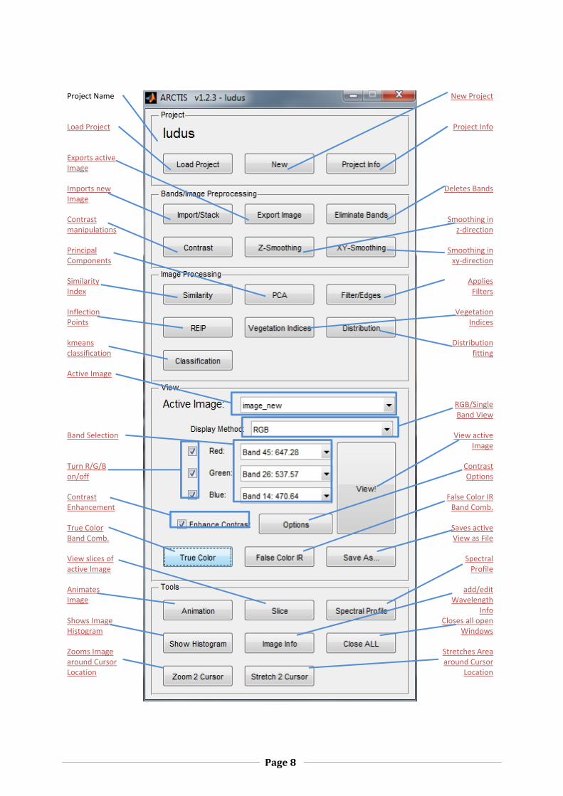
The GUI is divided in five sections as demonstrated in the screenshot below. The first section
contains functions for loading, creating and maintaining a project. It also displays the name of the
currently loaded project.
The second section provides image pre‐processing functions like importing/exporting an image, the
deletion of user‐specified bands, functions for contrast adjustment or 2 or 3‐dimensional smoothing.
Note: Smoothing of data – even if it takes a rather long time – is highly recommended as it increases
the quality of all subsequent analyses.
In the third section you find the main image processing functions: Similarity index calculation,
principal component analysis, filter and edge detection functions, inflection point calculation,
vegetation index calculation, distribution fitting and a simple classification algorithm. All these
functions produce new images with unique names which are stored in the image path of the current
project.
Page8
Project Name
New Project
Load Project Project Info
Exports active Image
Imports new Image
Deletes Bands
Contrast manipulations
Smoothing in z‐direction
Principal Components
Smoothing in xy‐direction
Similarity Index
AppliesFilters
Inflection Points
Vegetation Indices
kmeans classification
Distribution fitting
Active Image
RGB/Single Band View
Band Selection View active Image
Turn R/G/B on/off
Contrast Options
Contrast Enhancement
False Color IR Band Comb.
True Color Band Comb.
Saves active View as File
View slices of active Image
Spectral Profile
Animates Image
add/edit Wavelength
Info Shows Image Histogram
Closes all open Windows
Zooms Image around Cursor Location
Stretches Area around Cursor
Location
Page9
The fourth section provides the display controls and allows you to view your images. It contains the
drop‐down menu for selecting the active image, you can switch between single band and RGB display
mode, select which bands to display, decide whether or not you want to enhance the contrast of
your image before viewing it (and the way how to manipulate the contrast), you can select
predefined bands and you can save the your current view as a JPG or JPG2000 file. The functions in
this section do NOT change the data of your image; they just display the image using the selected
parameters.
The last section contains several tools which might help you during your image analysis: You
can display an animated sequence of your 3D data cube, view your data in slices, display
spectral profiles at selected points, show image histograms, add/edit wavelength information,
close all open ARCTIS windows and use the Zoom2Cursor and Stretch2Cursor functions to
highlight areas around the cursor automatically while you move it within the image frame.
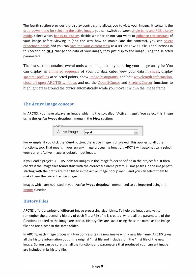
TheActiveImageconcept
In ARCTIS, you have always an image which is the so‐called “Active Image”. You select this image
using the Active Image dropdown menu in the View section:
For example, if you click the View! button, the active image is displayed. This applies to all other
functions, too. That means if you run any image processing function, ARCTIS will automatically select
your current Active Image as default input image.
If you load a project, ARCTIS looks for images in the image folder specified in the project file. It then
checks if the image files found start with the correct file name prefix. All image files in the image path
starting with the prefix are then listed in the active image popup menu and you can select them to
make them the current active image.
Images which are not listed in your Active Image dropdown menu need to be imported using the
Import function.
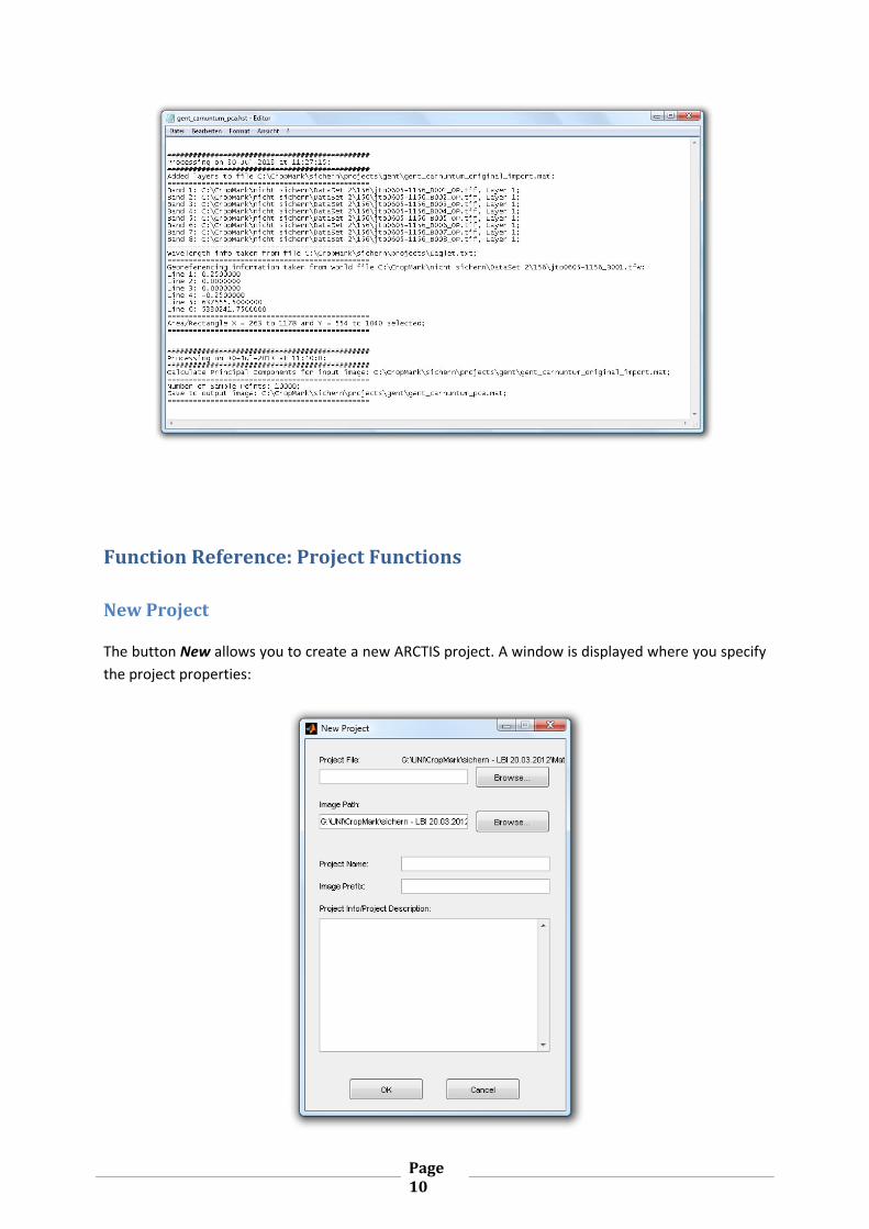
HistoryFiles
ARCTIS offers a variety of different image processing algorithms. To help the image analyst to
remember the processing history of each file, a *.hst file is created, where all the parameters of the
functions applied to the image are stored. History files are saved using the same name as the image
file and are placed in the same folder.
In ARCTIS, each image processing function results in a new image with a new file name. ARCTIS takes
all the history information out of the original *.hst file and includes it in the *.hst file of the new
image. So you can be sure that all the functions and parameters that produced your current image
are included in its history file.
Page10
FunctionReference:ProjectFunctions
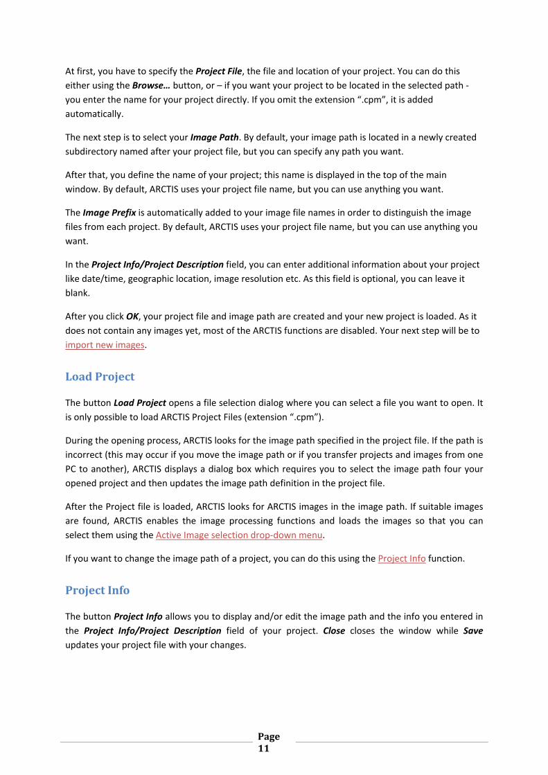
NewProject
The button New allows you to create a new ARCTIS project. A window is displayed where you specify
the project properties:
Page11
At first, you have to specify the Project File, the file and location of your project. You can do this
either using the Browse… button, or – if you want your project to be located in the selected path ‐
you enter the name for your project directly. If you omit the extension “.cpm”, it is added
automatically.
The next step is to select your Image Path. By default, your image path is located in a newly created
subdirectory named after your project file, but you can specify any path you want.
After that, you define the name of your project; this name is displayed in the top of the main
window. By default, ARCTIS uses your project file name, but you can use anything you want.
The Image Prefix is automatically added to your image file names in order to distinguish the image
files from each project. By default, ARCTIS uses your project file name, but you can use anything you
want.
In the Project Info/Project Description field, you can enter additional information about your project
like date/time, geographic location, image resolution etc. As this field is optional, you can leave it
blank.
After you click OK, your project file and image path are created and your new project is loaded. As it
does not contain any images yet, most of the ARCTIS functions are disabled. Your next step will be to
import new images.
LoadProject
The button Load Project opens a file selection dialog where you can select a file you want to open. It
is only possible to load ARCTIS Project Files (extension “.cpm”).
During the opening process, ARCTIS looks for the image path specified in the project file. If the path is
incorrect (this may occur if you move the image path or if you transfer projects and images from one
PC to another), ARCTIS displays a dialog box which requires you to select the image path four your
opened project and then updates the image path definition in the project file.
After the Project file is loaded, ARCTIS looks for ARCTIS images in the image path. If suitable images
are found, ARCTIS enables the image processing functions and loads the images so that you can
select them using the Active Image selection drop‐down menu.
If you want to change the image path of a project, you can do this using the Project Info function.
ProjectInfo
The button Project Info allows you to display and/or edit the image path and the info you entered in
the Project Info/Project Description field of your project. Close closes the window while Save
updates your project file with your changes.
Page12
FunctionReference:Bands/ImagePreprocessingFunctions
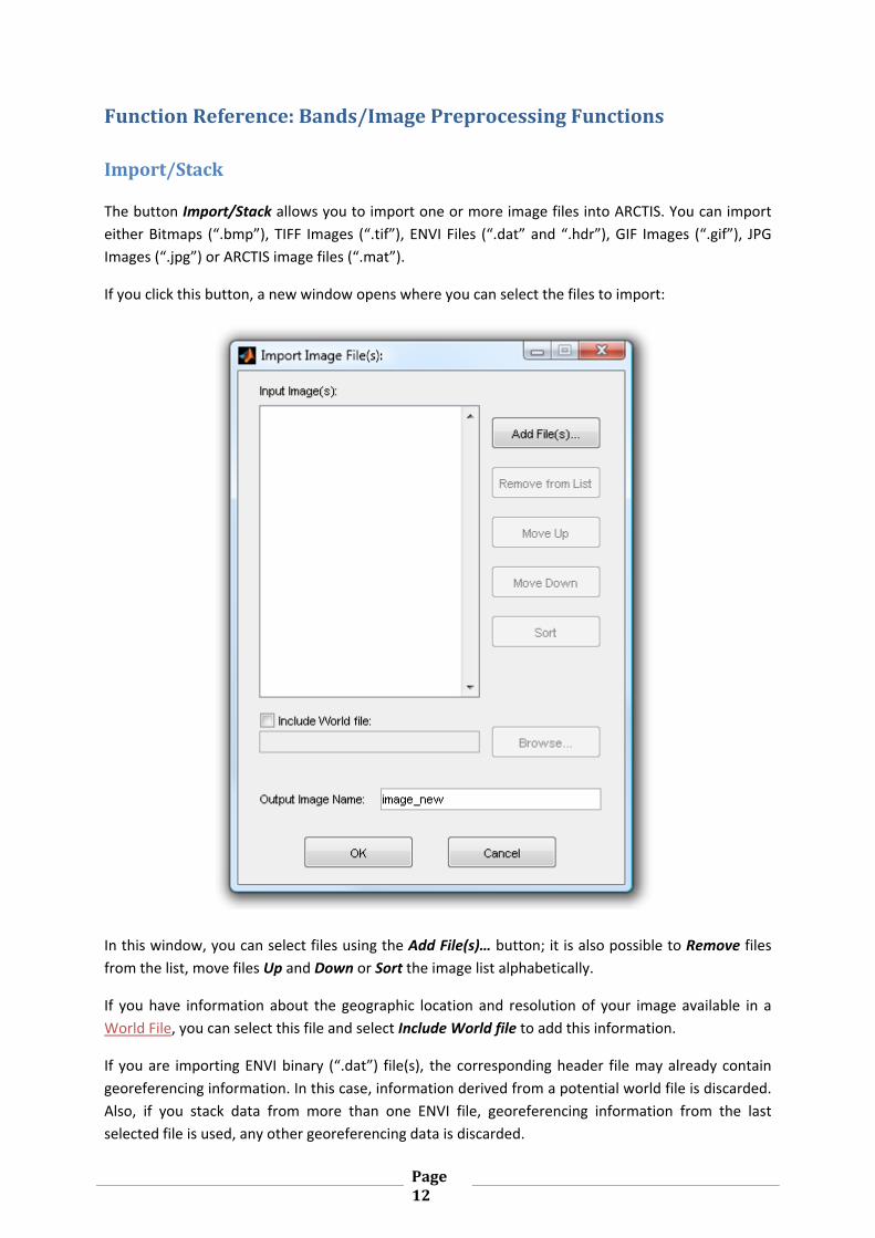
Import/Stack
The button Import/Stack allows you to import one or more image files into ARCTIS. You can import
either Bitmaps (“.bmp”), TIFF Images (“.tif”), ENVI Files (“.dat” and “.hdr”), GIF Images (“.gif”), JPG
Images (“.jpg”) or ARCTIS image files (“.mat”).
If you click this button, a new window opens where you can select the files to import:
In this window, you can select files using the Add File(s)… button; it is also possible to Remove files
from the list, move files Up and Down or Sort the image list alphabetically.
If you have information about the geographic location and resolution of your image available in a
World File, you can select this file and select Include World file to add this information.
If you are importing ENVI binary (“.dat”) file(s), the corresponding header file may already contain
georeferencing information. In this case, information derived from a potential world file is discarded.
Also, if you stack data from more than one ENVI file, georeferencing information from the last
selected file is used, any other georeferencing data is discarded.
Page13
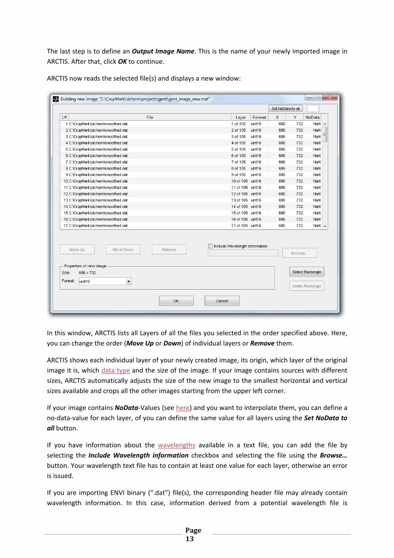
The last step is to define an Output Image Name. This is the name of your newly imported image in
ARCTIS. After that, click OK to continue.
ARCTIS now reads the selected file(s) and displays a new window:
In this window, ARCTIS lists all Layers of all the files you selected in the order specified above. Here,
you can change the order (Move Up or Down) of individual layers or Remove them.
ARCTIS shows each individual layer of your newly created image, its origin, which layer of the original
image it is, which data type and the size of the image. If your image contains sources with different
sizes, ARCTIS automatically adjusts the size of the new image to the smallest horizontal and vertical
sizes available and crops all the other images starting from the upper left corner.
If your image contains NoData‐Values (see here) and you want to interpolate them, you can define a
no‐data‐value for each layer, of you can define the same value for all layers using the Set NoData to
all button.
If you have information about the wavelengths available in a text file, you can add the file by
selecting the Include Wavelength information checkbox and selecting the file using the Browse…
button. Your wavelength text file has to contain at least one value for each layer, otherwise an error
is issued.
If you are importing ENVI binary (“.dat”) file(s), the corresponding header file may already contain
wavelength information. In this case, information derived from a potential wavelength file is
Page14
discarded. Also, if you stack data from more than one ENVI file, wavelength information from the last
selected file is used, any other wavelength data is discarded.
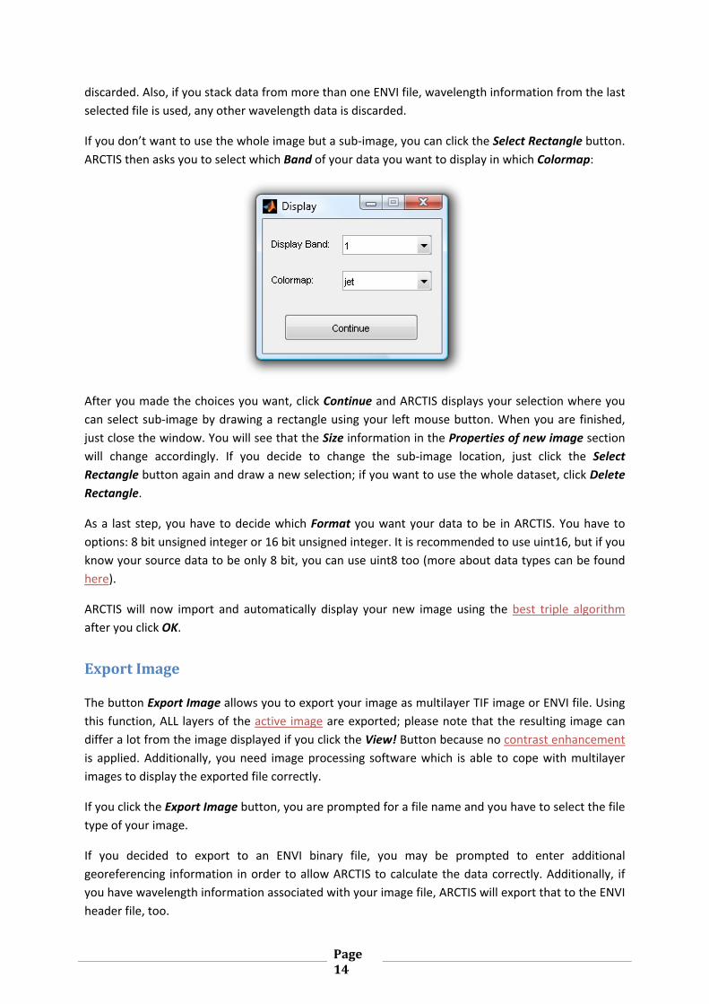
If you don’t want to use the whole image but a sub‐image, you can click the Select Rectangle button.
ARCTIS then asks you to select which Band of your data you want to display in which Colormap:
After you made the choices you want, click Continue and ARCTIS displays your selection where you
can select sub‐image by drawing a rectangle using your left mouse button. When you are finished,
just close the window. You will see that the Size information in the Properties of new image section
will change accordingly. If you decide to change the sub‐image location, just click the Select
Rectangle button again and draw a new selection; if you want to use the whole dataset, click Delete
Rectangle.
As a last step, you have to decide which Format you want your data to be in ARCTIS. You have to
options: 8 bit unsigned integer or 16 bit unsigned integer. It is recommended to use uint16, but if you
know your source data to be only 8 bit, you can use uint8 too (more about data types can be found
here).
ARCTIS will now import and automatically display your new image using the best triple algorithm
after you click OK.
ExportImage
The button Export Image allows you to export your image as multilayer TIF image or ENVI file. Using
this function, ALL layers of the active image are exported; please note that the resulting image can
differ a lot from the image displayed if you click the View! Button because no contrast enhancement
is applied. Additionally, you need image processing software which is able to cope with multilayer
images to display the exported file correctly.
If you click the Export Image button, you are prompted for a file name and you have to select the file
type of your image.
If you decided to export to an ENVI binary file, you may be prompted to enter additional
georeferencing information in order to allow ARCTIS to calculate the data correctly. Additionally, if
you have wavelength information associated with your image file, ARCTIS will export that to the ENVI
header file, too.
Page15
ARCTIS will then save your active image to the file you specified.
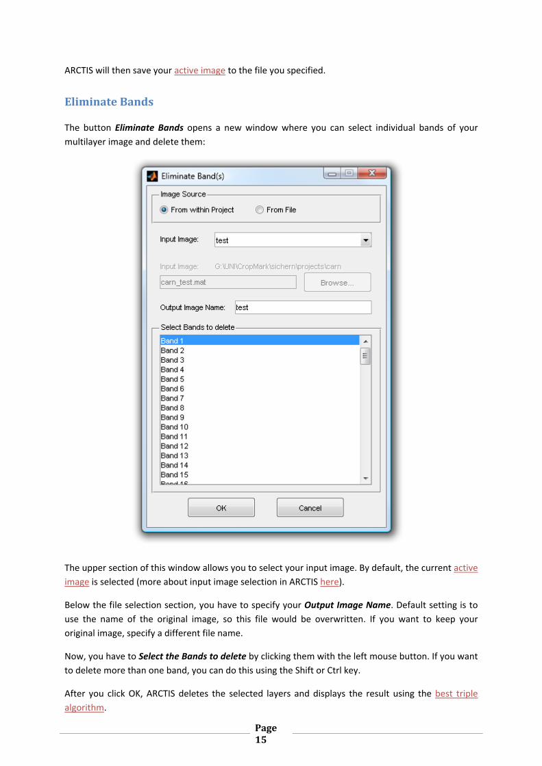
EliminateBands
The button Eliminate Bands opens a new window where you can select individual bands of your
multilayer image and delete them:
The upper section of this window allows you to select your input image. By default, the current active
image is selected (more about input image selection in ARCTIS here).
Below the file selection section, you have to specify your Output Image Name. Default setting is to
use the name of the original image, so this file would be overwritten. If you want to keep your
original image, specify a different file name.
Now, you have to Select the Bands to delete by clicking them with the left mouse button. If you want
to delete more than one band, you can do this using the Shift or Ctrl key.
After you click OK, ARCTIS deletes the selected layers and displays the result using the best triple
algorithm.
Page16
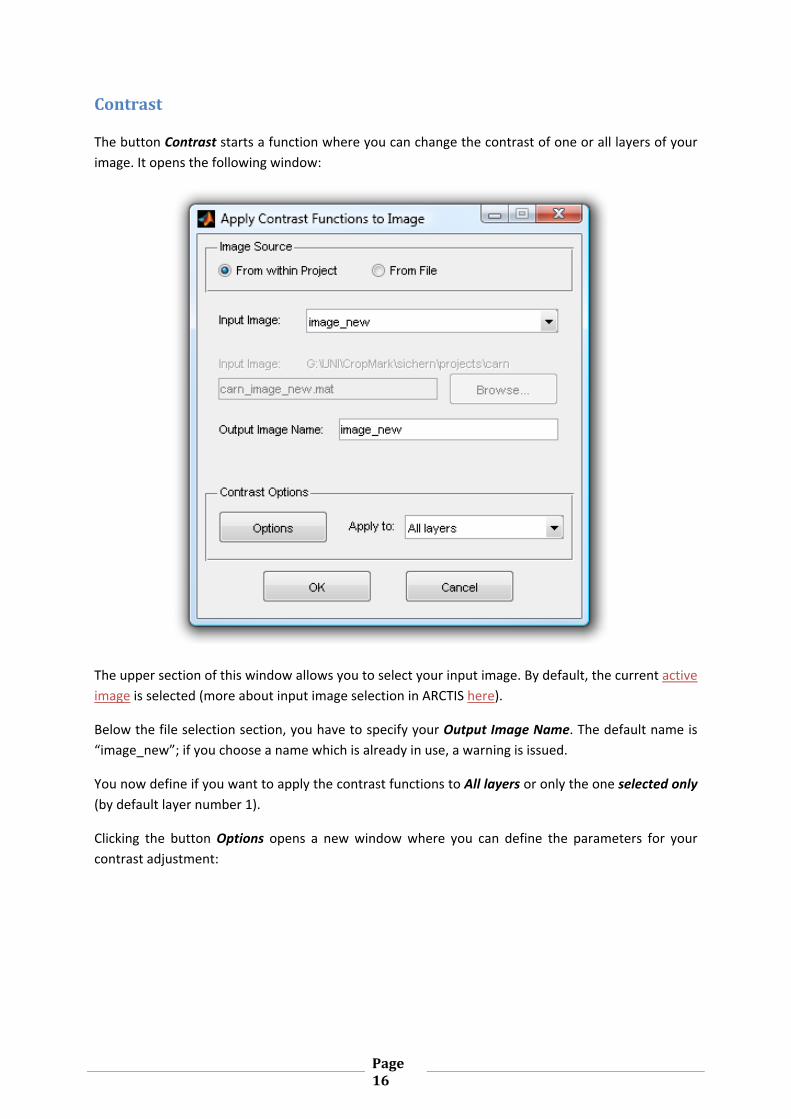
Contrast
The button Contrast starts a function where you can change the contrast of one or all layers of your
image. It opens the following window:
The upper section of this window allows you to select your input image. By default, the current active
image is selected (more about input image selection in ARCTIS here).
Below the file selection section, you have to specify your Output Image Name. The default name is
“image_new”; if you choose a name which is already in use, a warning is issued.
You now define if you want to apply the contrast functions to All layers or only the one selected only
(by default layer number 1).
Clicking the button Options opens a new window where you can define the parameters for your
contrast adjustment:
Page17
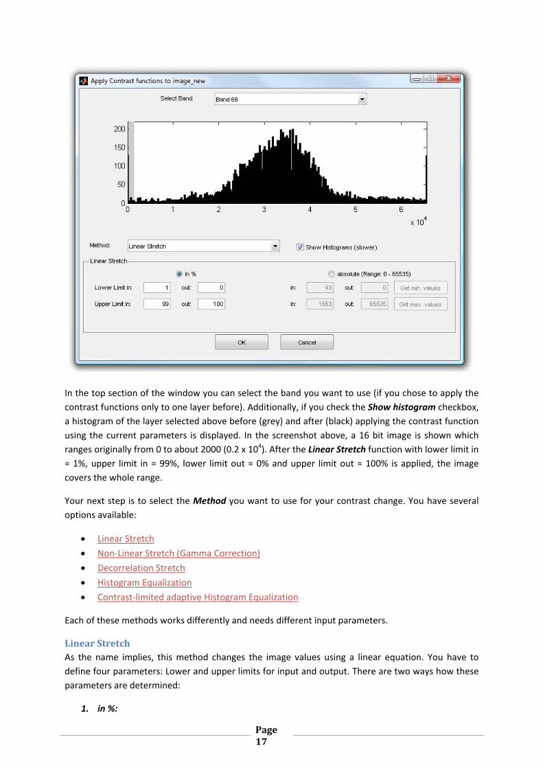
In the top section of the window you can select the band you want to use (if you chose to apply the
contrast functions only to one layer before). Additionally, if you check the Show histogram checkbox,
a histogram of the layer selected above before (grey) and after (black) applying the contrast function
using the current parameters is displayed. In the screenshot above, a 16 bit image is shown which
ranges originally from 0 to about 2000 (0.2 x 10⁴). After the Linear Stretch function with lower limit in
= 1%, upper limit in = 99%, lower limit out = 0% and upper limit out = 100% is applied, the image
covers the whole range.
Your next step is to select the Method you want to use for your contrast change. You have several
options available:
Linear Stretch
Non‐Linear Stretch (Gamma Correction)
Decorrelation Stretch
Histogram Equalization
Contrast‐limited adaptive Histogram Equalization
Each of these methods works differently and needs different input parameters.
LinearStretchAs the name implies, this method changes the image values using a linear equation. You have to
define four parameters: Lower and upper limits for input and output. There are two ways how these
parameters are determined:
1. in %:
Page18
You can define the input and output limits as a fractile in percent. Note that while output
limits stay the same for each layer and are only determined by the data type (see here; if you
set the output limit to 50% and are using 16 bit images which range from 0 to 65535, ARCTIS
calculates 50% = 32768), the input limits vary from layer to layer as they are determined by
the layer histogram.
The advantage of the percentage input is that you obtain an image which uses the same
value range in each layer. But, of course, dependencies between the layers are removed,
especially if the value range of the input layers varies widely. So if you want to keep the
correct relationship between the layers, it is recommended to use the second way of
determining input and output limits:
2. absolute values:
You also can define the input and output limit values directly using the absolute method. This
method applies the same formula to all layers, so the relationship between the layers is kept.
You have the possibility to automatically obtain the minimum and maximum values of your
whole image (not layer!) by clicking the correspondent buttons. If you use these values, the
resulting image covers the whole range (depending on the data type); if your image has 16
bit, the lowest value of all layers will be 0 and the highest 65535.
ARCTIS now calculates the output values applying the linear equation
∗
to each pixel where
inij = input pixel values outij = output pixel values lin = lower limit in for the current layer uin = upper limit in for the current layer lout = lower limit out for the current layer uout = upper limit out for the current layer.
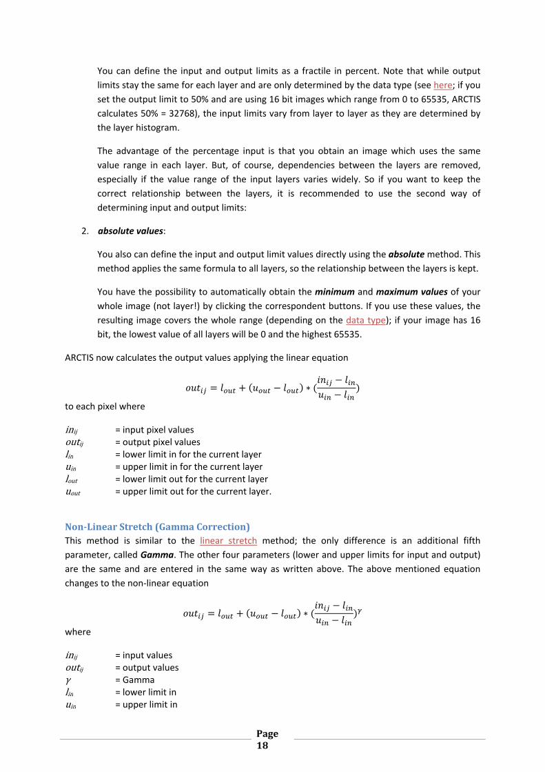
Non‐LinearStretch(GammaCorrection)This method is similar to the linear stretch method; the only difference is an additional fifth
parameter, called Gamma. The other four parameters (lower and upper limits for input and output)
are the same and are entered in the same way as written above. The above mentioned equation
changes to the non‐linear equation
∗
where
inij = input values outij = output values γ = Gamma lin = lower limit in uin = upper limit in
Page19
lout = lower limit out uout = upper limit out.
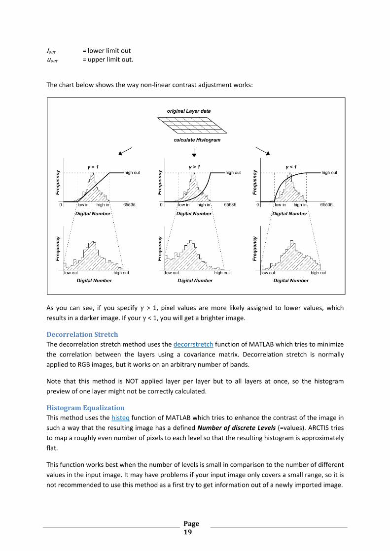
The chart below shows the way non‐linear contrast adjustment works:
As you can see, if you specify γ > 1, pixel values are more likely assigned to lower values, which
results in a darker image. If your γ < 1, you will get a brighter image.
DecorrelationStretchThe decorrelation stretch method uses the decorrstretch function of MATLAB which tries to minimize
the correlation between the layers using a covariance matrix. Decorrelation stretch is normally
applied to RGB images, but it works on an arbitrary number of bands.
Note that this method is NOT applied layer per layer but to all layers at once, so the histogram
preview of one layer might not be correctly calculated.
HistogramEqualizationThis method uses the histeq function of MATLAB which tries to enhance the contrast of the image in
such a way that the resulting image has a defined Number of discrete Levels (=values). ARCTIS tries
to map a roughly even number of pixels to each level so that the resulting histogram is approximately
flat.
This function works best when the number of levels is small in comparison to the number of different
values in the input image. It may have problems if your input image only covers a small range, so it is
not recommended to use this method as a first try to get information out of a newly imported image.
Page20
Contrast‐limitedadaptiveHistogramEqualization(CLAHE)This method uses the adapthisteq function of MATLAB. This function operates on small regions called
tiles, which sizes are determined through the Number of Tiles (Row x Column) you define. The
contrast of each tile is enhanced in a way that it fits the specified Distribution: uniform results in a
flat histogram, rayleigh in a Bell‐shaped curve and exponential in a curved histogram. The
neighboring tiles are then combined using bilinear interpolation to eliminate artificially induced
boundaries.
Other parameters you can define are
Clip Limit: This number specifies a limit for contrast enhancement. It ranges from 0 to 1;
higher numbers result in more contrast.
Number of Bins: This value specifies the number of bins used during histogram calculation.
Higher values result in greater dynamic range but in slower processing speed.
Range: You can specify if your output image should cover the full possible range (0…65535 if
you are working on a 16 bit image) or if ARCTIS should keep the range of the original image.
Alpha (only used when Distribution is set to rayleigh or exponential): Distribution parameter
If you have entered your contrast enhancement settings, save them by clicking OK. Pressing OK again
on the Apply Contrast Functions to Image window starts the process. If the calculation is finished,
ARCTIS displays your newly created image using the best triple algorithm.
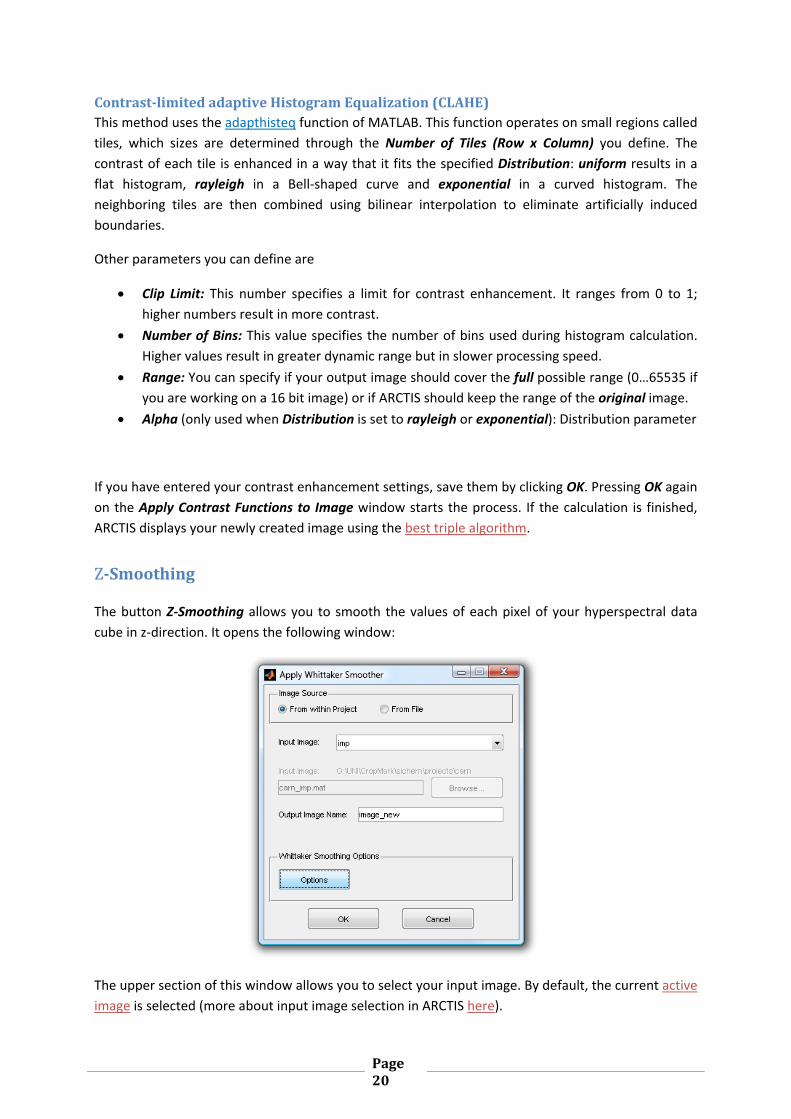
Z‐Smoothing
The button Z‐Smoothing allows you to smooth the values of each pixel of your hyperspectral data
cube in z‐direction. It opens the following window:
The upper section of this window allows you to select your input image. By default, the current active
image is selected (more about input image selection in ARCTIS here).

Page21
Below the file selection section, you have to specify your Output Image Name. The default name is
“image_new”; if you choose a name which is already in use, a warning is issued.
Clicking the button Options opens a new window where you can define the smoothing parameter:
This window displays the values of each layer for a certain point. ARCTIS selects the center point of
your image by default, but you can display every other point if you want to by clicking the Get Point…
button (which starts the point selection tool) or by entering the X and Y value of your desired point
directly.
ARCTIS displays the original profile in blue, calculates the smoothed values using the current
smoothing parameter and shows the result in red. The smoothing parameter λ ranges from ‐4 to 6,
with 1 being the default value. You can change λ using the slider or enter your desired value directly. As you do so, ARCTIS will adjust the graph accordingly.
Clicking OK saves the smoothing parameters; clicking OK again starts the smoothing function. ARCTIS
calculates the new image and displays it using the best triple algorithm afterwards.
The chart below shows the principle of the smoothing process:
Page22
ARCTIS calculates the smoothed image pixel per pixel; for every pixel location, all the layer values are
taken, smoothed values are calculated and written into a new image. Especially if you are working
with larger images, the smoothing process may take a while.
The smoothing algorithm used in ARCTIS was originally developed by Whittaker (Whittaker, 1923)
and modified and implemented in MATLAB by Paul Eilers (Eilers, 2003). For a detailed explanation of
the mathematical background, please refer to the original documents.
Please note that the smoother in ARCTIS treats all bands as if they were equally spaced in the
wavelength range.
It is strongly recommended to apply the Z‐Smoothing algorithm to each image as a second step after
importing.
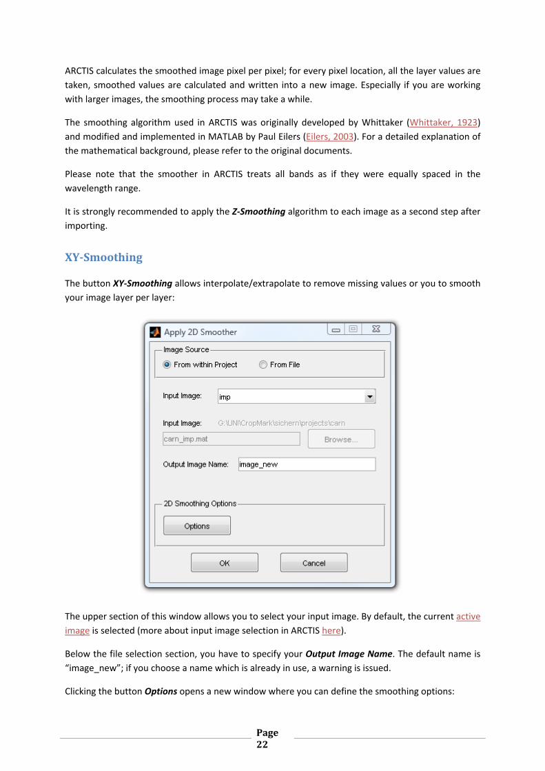
XY‐Smoothing
The button XY‐Smoothing allows interpolate/extrapolate to remove missing values or you to smooth
your image layer per layer:
The upper section of this window allows you to select your input image. By default, the current active
image is selected (more about input image selection in ARCTIS here).
Below the file selection section, you have to specify your Output Image Name. The default name is
“image_new”; if you choose a name which is already in use, a warning is issued.
Clicking the button Options opens a new window where you can define the smoothing options:
Page23
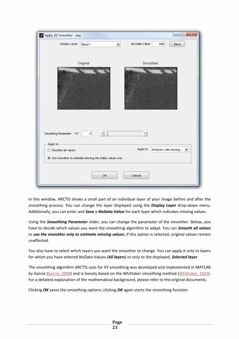
In this window, ARCTIS shows a small part of an individual layer of your image before and after the
smoothing process. You can change the layer displayed using the Display Layer drop‐down menu.
Additionally, you can enter and Save a NoData‐Value for each layer which indicates missing values.
Using the Smoothing Parameter slider, you can change the parameter of the smoother. Below, you
have to decide which values you want the smoothing algorithm to adapt. You can Smooth all values
or use the smoother only to estimate missing values; if this option is selected, original values remain
unaffected.
You also have to select which layers you want the smoother to change. You can apply it only to layers
for which you have entered NoData‐Values (All layers) or only to the displayed, Selected layer.
The smoothing algorithm ARCTIS uses for XY‐smoothing was developed and implemented in MATLAB
by Garcia (Garcia, 2009) and is loosely based on the Whittaker smoothing method (Whittaker, 1923).
For a detailed explanation of the mathematical background, please refer to the original documents.
Clicking OK saves the smoothing options; clicking OK again starts the smoothing function.
Page24
FunctionReference:ImageProcessingFunctions
Similarity
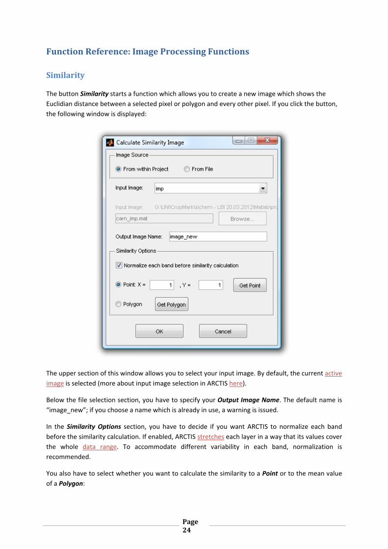
The button Similarity starts a function which allows you to create a new image which shows the
Euclidian distance between a selected pixel or polygon and every other pixel. If you click the button,
the following window is displayed:
The upper section of this window allows you to select your input image. By default, the current active
image is selected (more about input image selection in ARCTIS here).
Below the file selection section, you have to specify your Output Image Name. The default name is
“image_new”; if you choose a name which is already in use, a warning is issued.
In the Similarity Options section, you have to decide if you want ARCTIS to normalize each band
before the similarity calculation. If enabled, ARCTIS stretches each layer in a way that its values cover
the whole data range. To accommodate different variability in each band, normalization is
recommended.
You also have to select whether you want to calculate the similarity to a Point or to the mean value
of a Polygon:
Page25
Similarity to a point: Select the point you want using the Get Point button (more about point
selection here) or enter the X and Y values directly.
ARCTIS calculates the Euclidian distance using the formula
,
where
inlayer,ij = input pixel values of each layer outij = output pixel values n = number of layers player = pixel value to which the similarity is calculated.
Similarity to the mean of a polygon: Select a polygon using the Get Polygon button (more
about polygon selection here).
ARCTIS calculates the Euclidian distance using the formula
,1
,
where
inlayer,ij = input pixel values of each layer outij = output pixel values n = number of layers k = number polygon pixels player,m = pixel values of the polygon to which the similarity is calculated to.
If you click OK, ARCTIS starts the calculation using the formulas above. Then the output values are
normalized so that they range from 0 to 1 and subtracted from 1 in order to get a resulting image
where the lowest similarity is 0 and the highest 1. As a last step, the resulting image is stretched to
cover the whole available range, and then displayed.
PrincipalComponentAnalysis(PCA)
The button PCA starts a function which is able to calculate the principal components of an input
image. If you click the button, the following window is displayed:
The upper section of this window allows you to select your input image. By default, the current active
image is selected (more about input image selection in ARCTIS here).
Below the file selection section, you have to specify your Output Image Name. The default name is
“image_new”; if you choose a name which is already in use, a warning is issued.
Principal Component Analysis is an often effective method to reduce the amount of data by
“compressing” the available information into an image with fewer layers and appeared for example
in the work of Pearson (Pearson, 1901).
Page26
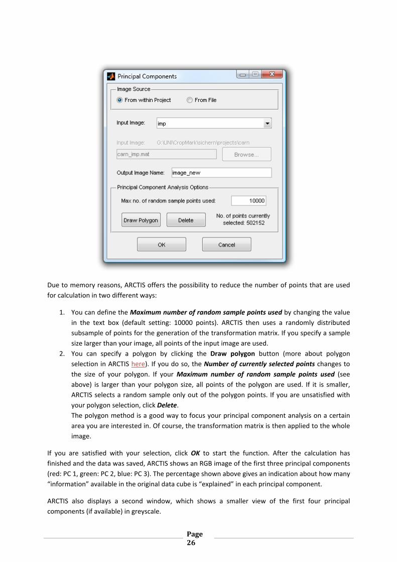
Due to memory reasons, ARCTIS offers the possibility to reduce the number of points that are used
for calculation in two different ways:
1. You can define the Maximum number of random sample points used by changing the value
in the text box (default setting: 10000 points). ARCTIS then uses a randomly distributed
subsample of points for the generation of the transformation matrix. If you specify a sample
size larger than your image, all points of the input image are used.
2. You can specify a polygon by clicking the Draw polygon button (more about polygon
selection in ARCTIS here). If you do so, the Number of currently selected points changes to
the size of your polygon. If your Maximum number of random sample points used (see
above) is larger than your polygon size, all points of the polygon are used. If it is smaller,
ARCTIS selects a random sample only out of the polygon points. If you are unsatisfied with
your polygon selection, click Delete.
The polygon method is a good way to focus your principal component analysis on a certain
area you are interested in. Of course, the transformation matrix is then applied to the whole
image.
If you are satisfied with your selection, click OK to start the function. After the calculation has
finished and the data was saved, ARCTIS shows an RGB image of the first three principal components
(red: PC 1, green: PC 2, blue: PC 3). The percentage shown above gives an indication about how many
“information” available in the original data cube is “explained” in each principal component.
ARCTIS also displays a second window, which shows a smaller view of the first four principal
components (if available) in greyscale.

Page27
Filter/Edges
The button Filter/Edges starts a function which allows you to apply several filtering techniques or
edge detection algorithms to your image. If you click the button, the following window is displayed:
The upper section of this window allows you to select your input image. By default, the current active
image is selected (more about input image selection in ARCTIS here).
Below the file selection section, you have to specify your Output Image Name. The default name is
“image_new”; if you choose a name which is already in use, a warning is issued.
ARCTIS offers three different Filter Methods with different parameters:
1. N‐D‐Filtering
2. 2‐D‐Adaptive noise removal filtering (Wiener Method)
3. Edge Detection
Page28
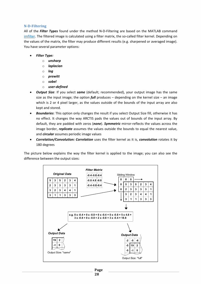
N‐D‐FilteringAll of the Filter Types found under the method N‐D‐Filtering are based on the MATLAB command
imfilter. The filtered image is calculated using a filter matrix, the so‐called filter kernel. Depending on
the values of the matrix, the filter may produce different results (e.g. sharpened or averaged image).
You have several parameter options:
Filter Type:
o unsharp
o laplacian
o log
o prewitt
o sobel
o user‐defined
Output Size: If you select same (default; recommended), your output image has the same
size as the input image; the option full produces – depending on the kernel size – an image
which is 2 or 4 pixel larger, as the values outside of the bounds of the input array are also
kept and stored.
Boundaries: This option only changes the result if you select Output Size fill, otherwise it has
no effect. It changes the way ARCTIS pads the values out of bounds of the input array. By
default, they are padded with zeros (none). Symmetric mirror‐reflects the values across the
image border, replicate assumes the values outside the bounds to equal the nearest value,
and circular assumes periodic image values
Correlation/Convolution: Correlation uses the filter kernel as it is, convolution rotates it by
180 degrees
The picture below explains the way the filter kernel is applied to the image; you can also see the
difference between the output sizes:
Page29
The negative values occurring in this example are eliminated by stretching the resulting image layers
to range from 0 to 255 (uint8) or 0 to 65535 (uint16).
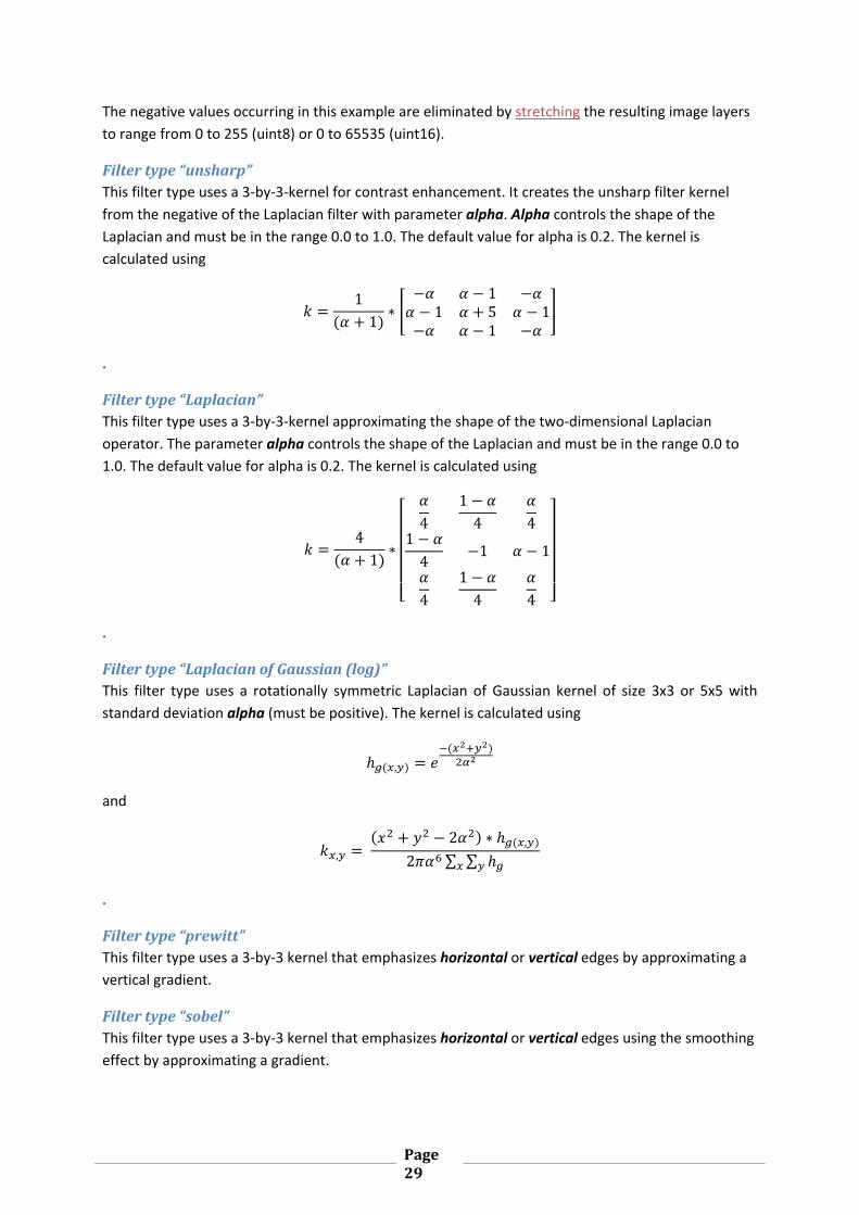
Filtertype“unsharp”This filter type uses a 3‐by‐3‐kernel for contrast enhancement. It creates the unsharp filter kernel
from the negative of the Laplacian filter with parameter alpha. Alpha controls the shape of the
Laplacian and must be in the range 0.0 to 1.0. The default value for alpha is 0.2. The kernel is
calculated using
11∗
11 5 1
1
.
Filtertype“Laplacian”This filter type uses a 3‐by‐3‐kernel approximating the shape of the two‐dimensional Laplacian
operator. The parameter alpha controls the shape of the Laplacian and must be in the range 0.0 to
1.0. The default value for alpha is 0.2. The kernel is calculated using
41∗
414 4
14
1 1
414 4
.
Filtertype“LaplacianofGaussian(log)”This filter type uses a rotationally symmetric Laplacian of Gaussian kernel of size 3x3 or 5x5 with
standard deviation alpha (must be positive). The kernel is calculated using
,
and
, 2 ∗ ,
2 ∑ ∑
.
Filtertype“prewitt”This filter type uses a 3‐by‐3 kernel that emphasizes horizontal or vertical edges by approximating a
vertical gradient.
Filtertype“sobel”This filter type uses a 3‐by‐3 kernel that emphasizes horizontal or vertical edges using the smoothing
effect by approximating a gradient.
Page30
Filtertype“user‐defined”This filter type allows you to define your own 3‐by‐3 or 5‐by‐5 kernel which is then applied to the
image.
2D‐adaptivenoiseremovalfiltering(Wienermethod)This method lowpass‐filters each layer image as if it has been degraded by constant power additive
noise. It2 uses a pixelwise adaptive Wiener method based on statistics estimated from a local
neighborhood of each pixel. You have to specify the Size of the neighborhood used to estimate the
local image mean and standard deviation.
ARCTIS calculates the local mean and variance around each pixel:
1² ,
and
²1² , ² ²
where N is the neighborhood size. It then creates a pixel‐wise Wiener filter using these estimates,
,
where ν² equals the average of all the local estimated variances.
EdgedetectionThis method allows you to apply several edge detection algorithms to your image. Edge detection
algorithms try to locate edges in each layer of the input images. The resulting output image consists
of as many layers as the input image and is in binary format where 0 = no edge found and 1 = edge
found. If you check the Generate Sum Image option, an additional image is produced which
represents the sum of all the edge layers. It is stored in the project folder and named [image
name]_sum.
Several different edge detection methods are implemented in ARCTIS which require different
parameters:
Method“sobel”The sobel method uses the sobel operator to calculate the image gradient. If you set a Threshold
value, all edges not stronger than this value are ignored. Otherwise, the threshold value is chosen
automatically.
You can also set the Direction of the edges you want ARCTIS to look for (horizontal, vertical or both).
Additionally, you can choose to skip an optional edge thinning stage (nothinning) or apply it
(thinning).
Method“canny”The canny method applies two thresholds to the gradient: a high threshold for low edge sensitivity
and a low threshold for high edge sensitivity. It starts with the low sensitivity result and then grows it
Page31
to include connected edge pixels from the high sensitivity result. This helps fill in gaps in the detected
edges (MATLAB Docs).
Sigma represents the standard deviation of the Gaussian filter. MATLAB chooses the size of the filter
automatically based on the value of sigma.
Method“LaplacianofGaussian”This method uses the Laplacian of Gaussian approach for edge detection.
Sigma represents the standard deviation of the Laplacian of Gaussian filter. MATLAB chooses the size
of the filter automatically based on the value of sigma.
Method“roberts”The roberts method uses equations proposed by Lawrence Roberts (Roberts, 1963). If you set a
Threshold value, all edges not stronger than this value are ignored. Otherwise, the threshold value is
chosen automatically.
Additionally, you can choose to skip an optional edge thinning stage (nothinning) or apply it
(thinning).
Method“zerocross”This method uses a zero cross approach for edge detection. If you set a Threshold value, all edges not
stronger than this value are ignored. Otherwise, the threshold value is chosen automatically.
Additionally, you can choose to skip an optional edge thinning stage (nothinning) or apply it
(thinning).
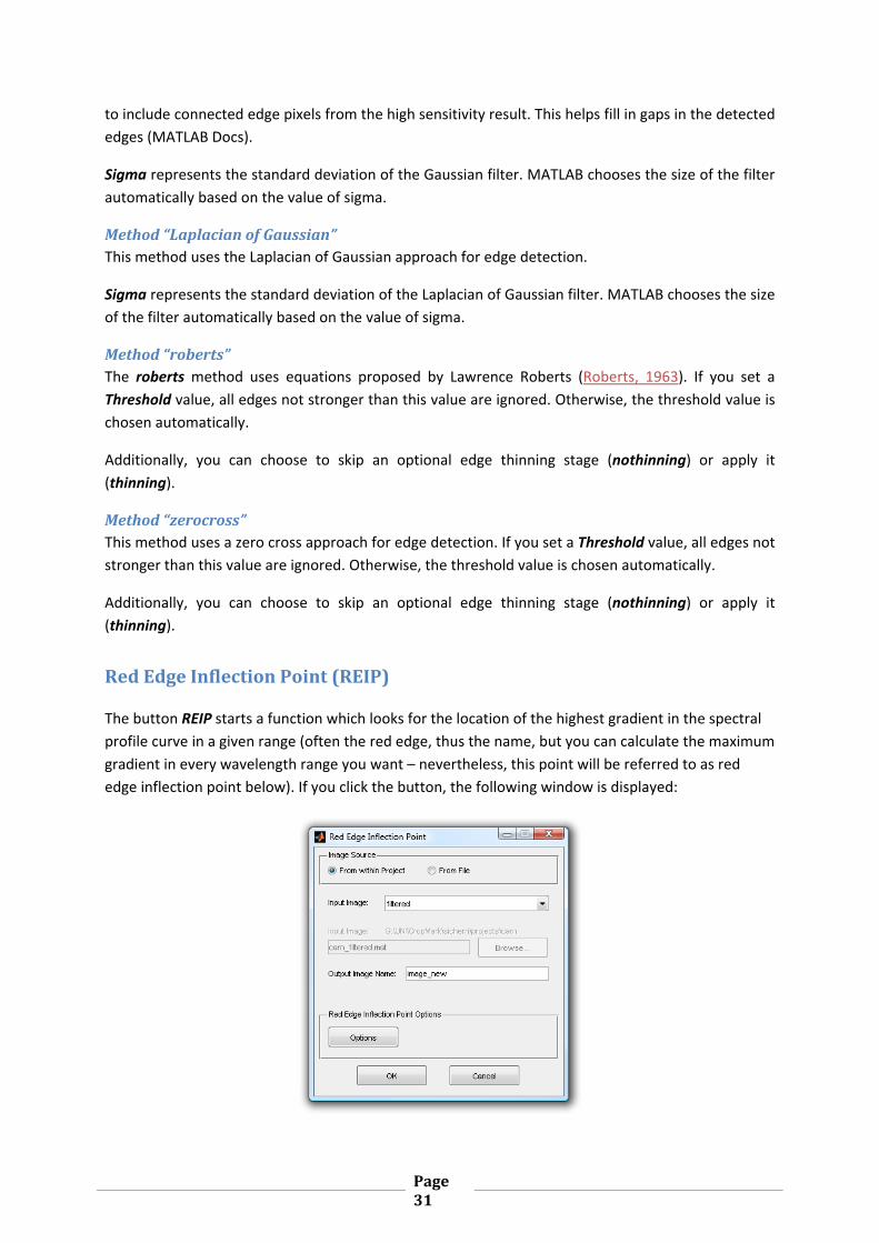
RedEdgeInflectionPoint(REIP)
The button REIP starts a function which looks for the location of the highest gradient in the spectral
profile curve in a given range (often the red edge, thus the name, but you can calculate the maximum
gradient in every wavelength range you want – nevertheless, this point will be referred to as red
edge inflection point below). If you click the button, the following window is displayed:
Page32
The upper section of this window allows you to select your input image. By default, the current active
image is selected (more about input image selection in ARCTIS here).
Below the file selection section, you have to specify your Output Image Name. The default name is
“image_new”; if you choose a name which is already in use, a warning is issued.
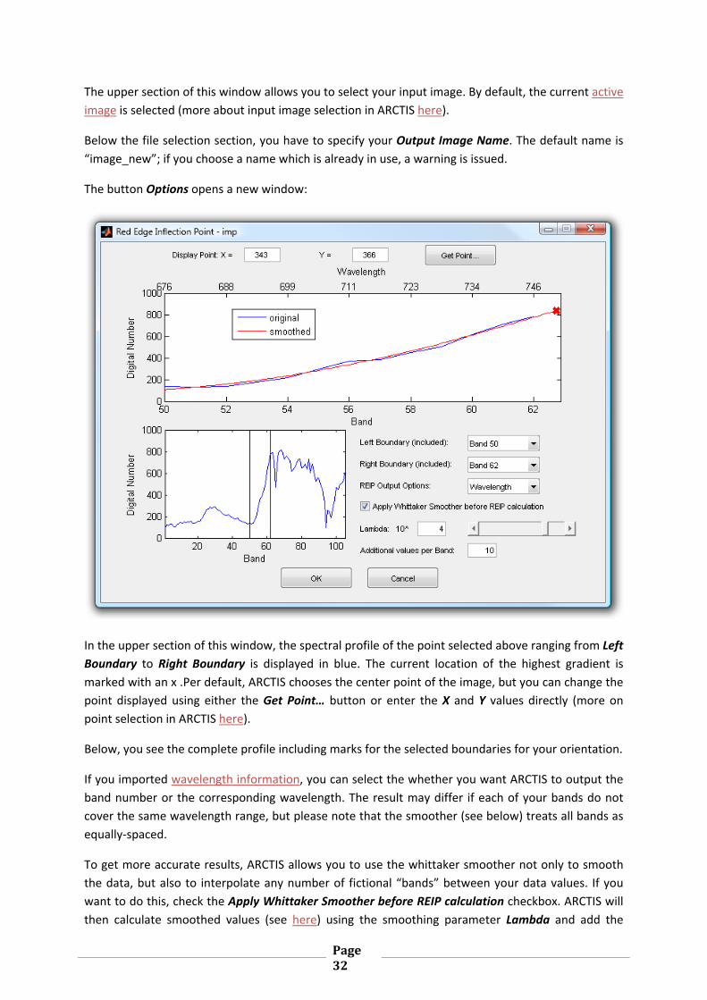
The button Options opens a new window:
In the upper section of this window, the spectral profile of the point selected above ranging from Left
Boundary to Right Boundary is displayed in blue. The current location of the highest gradient is
marked with an x .Per default, ARCTIS chooses the center point of the image, but you can change the
point displayed using either the Get Point… button or enter the X and Y values directly (more on
point selection in ARCTIS here).
Below, you see the complete profile including marks for the selected boundaries for your orientation.
If you imported wavelength information, you can select the whether you want ARCTIS to output the
band number or the corresponding wavelength. The result may differ if each of your bands do not
cover the same wavelength range, but please note that the smoother (see below) treats all bands as
equally‐spaced.
To get more accurate results, ARCTIS allows you to use the whittaker smoother not only to smooth
the data, but also to interpolate any number of fictional “bands” between your data values. If you
want to do this, check the Apply Whittaker Smoother before REIP calculation checkbox. ARCTIS will
then calculate smoothed values (see here) using the smoothing parameter Lambda and add the
Page33
number of bands specified in Additional values per band. Please note that you may have to adjust
the smoothing parameter each time you change the number of additional values per band.
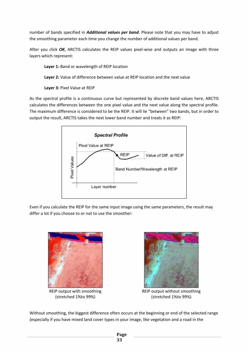
After you click OK, ARCTIS calculates the REIP values pixel‐wise and outputs an image with three
layers which represent:
Layer 1: Band or wavelength of REIP location
Layer 2: Value of difference between value at REIP location and the next value
Layer 3: Pixel Value at REIP
As the spectral profile is a continuous curve but represented by discrete band values here, ARCTIS
calculates the differences between the one pixel value and the next value along the spectral profile.
The maximum difference is considered to be the REIP. It will lie “between” two bands, but in order to
output the result, ARCTIS takes the next lower band number and treats it as REIP:
Even if you calculate the REIP for the same input image using the same parameters, the result may
differ a lot if you choose to or not to use the smoother:
REIP output with smoothing
(stretched 1%to 99%) REIP output without smoothing
(stretched 1%to 99%)
Without smoothing, the biggest difference often occurs at the beginning or end of the selected range
(especially if you have mixed land cover types in your image, like vegetation and a road in the
Page34
example above), so the REIP is found at the lowest or highest band number. With smoothing (and
interpolation), the profile at the edges of the selected range may look very different and the REIP is
found somewhere else.
ARCTIS looks for the maximum difference regardless of the difference being positive or negative, but
for the result in layer 2 (value of difference) the sign is taken into consideration.
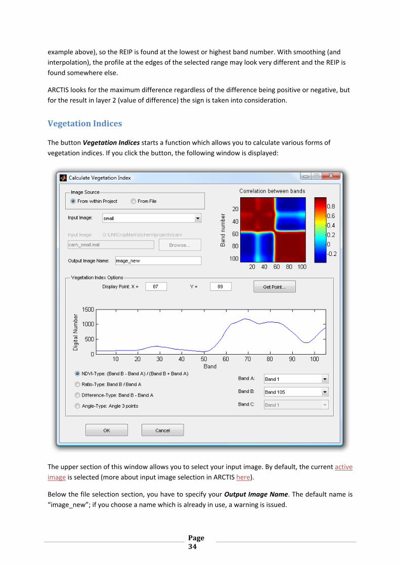
VegetationIndices
The button Vegetation Indices starts a function which allows you to calculate various forms of
vegetation indices. If you click the button, the following window is displayed:
The upper section of this window allows you to select your input image. By default, the current active
image is selected (more about input image selection in ARCTIS here).
Below the file selection section, you have to specify your Output Image Name. The default name is
“image_new”; if you choose a name which is already in use, a warning is issued.
Page35
On the upper right corner of the window, ARCTIS displays the correlation matrix between the bands
of your image. It is designed to help you decide which bands you use for calculating a vegetation
index; if you use two highly‐correlated bands, the results may not be useful.
Below, the spectral profile of the point selected above is displayed in blue. Per default, ARCTIS
chooses the center point of the image, but you can change the point displayed using either the Get
Point… button or enter the X and Y values directly (more on point selection in ARCTIS here).
Below, you can select which bands you want to use as Band A, B and C for your vegetation index
calculation and which of these for index types you want to calculate:
NDVI‐TypeFor NDVI‐type (Normalized Difference Vegetation Index) vegetation indices, the output value for
each pixel is calculated using the formula
where
outij = output pixel values aij = Band A Pixel values bij = Band B pixel values.
Ratio‐typeFor ratio‐type vegetation indices, the output value for each pixel is calculated using the formula
where
outij = output pixel values aij = Band A Pixel values bij = Band B pixel values.
Difference‐typeFor difference‐type vegetation indices, the output value for each pixel is calculated using the formula
where
outij = output pixel values aij = Band A Pixel values bij = Band B pixel values.
Page36
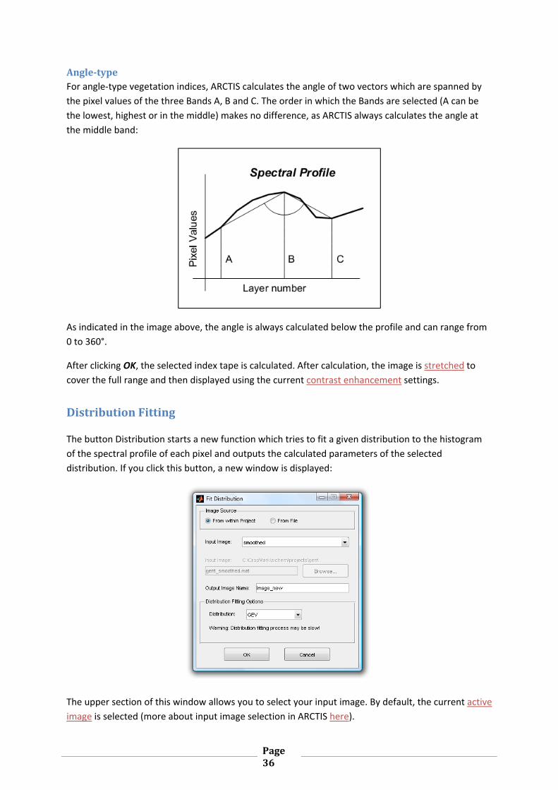
Angle‐typeFor angle‐type vegetation indices, ARCTIS calculates the angle of two vectors which are spanned by
the pixel values of the three Bands A, B and C. The order in which the Bands are selected (A can be
the lowest, highest or in the middle) makes no difference, as ARCTIS always calculates the angle at
the middle band:
As indicated in the image above, the angle is always calculated below the profile and can range from
0 to 360°.
After clicking OK, the selected index tape is calculated. After calculation, the image is stretched to
cover the full range and then displayed using the current contrast enhancement settings.
DistributionFitting
The button Distribution starts a new function which tries to fit a given distribution to the histogram
of the spectral profile of each pixel and outputs the calculated parameters of the selected
distribution. If you click this button, a new window is displayed:
The upper section of this window allows you to select your input image. By default, the current active
image is selected (more about input image selection in ARCTIS here).
Page37
Below the file selection section, you have to specify your Output Image Name. The default name is
“image_new”; if you choose a name which is already in use, a warning is issued.
Below, you can select which Distribution you want to fit to your data. After clicking OK, ARCTIS
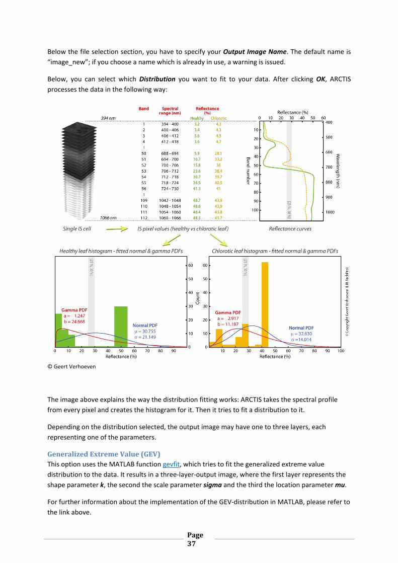
processes the data in the following way:
© Geert Verhoeven
The image above explains the way the distribution fitting works: ARCTIS takes the spectral profile
from every pixel and creates the histogram for it. Then it tries to fit a distribution to it.
Depending on the distribution selected, the output image may have one to three layers, each
representing one of the parameters.
GeneralizedExtremeValue(GEV)This option uses the MATLAB function gevfit, which tries to fit the generalized extreme value
distribution to the data. It results in a three‐layer‐output image, where the first layer represents the
shape parameter k, the second the scale parameter sigma and the third the location parameter mu.
For further information about the implementation of the GEV‐distribution in MATLAB, please refer to
the link above.

Page38
WeibullThis option uses the MATLAB function wblfit, which tries to fit the Weibull distribution to the data. It
results in a two‐layer‐output image, where the first layer represents the Weibull parameter a, the
second the parameter b.
For further information about the implementation of the Weibull distribution in MATLAB, please
refer to the link above.
PoissonThis option uses the MATLAB function poissfit, which tries to fit the Poisson distribution to the data.
It results in a one‐layer‐output image which represents the Poisson parameter lambda.
For further information about the implementation of the Poisson distribution in MATLAB, please
refer to the link above.
NormalThis option uses the MATLAB function normfit, which tries to fit the normal distribution to the data.
It results in a four‐layer‐output image, where the first layer represents the mean value µ, the second
the standard deviation sigma and the third and the fourth the lower and upper bound of the
confidence interval for µ.
For further information about the implementation of the normal distribution in MATLAB, please refer
to the link above.
Log‐NormalThis option uses the MATLAB function lognfit, which tries to fit the lognormal distribution to the
data. It results in a two‐layer‐output image, where the first layer represents the mean value µ, the
second the standard deviation sigma.
For further information about the implementation of the lognormal distribution in MATLAB, please
refer to the link above.
BetaThis option uses the MATLAB function betafit, which tries to fit the beta distribution to the data. It
results in a two‐layer‐output image, where the first layer represents the parameter a, the second the
parameter b.
For further information about the implementation of the beta distribution in MATLAB, please refer to
the link above.
GammaThis option uses the MATLAB function gamfit, which tries to fit the gamma distribution to the data. It
results in a two‐layer‐output image, where the first layer represents the parameter a, the second the
parameter b.
For further information about the implementation of the gamma distribution in MATLAB, please
refer to the link above.
Page39
There is no indication of how well the selected distribution fits to the given input data, and ARCTIS
will always return a result, even if the fitted distribution does not fit at all to the input histogram. So
this function is to be seen as an attempt to look at the data in a new and different way, not to find
possible common distributions in the data.
Please also note that for some distributions, the fitting process uses an iterative algorithm which – as
it needs to be applied pixel‐wise – can be very time‐consuming.
After the calculation of the parameters, each layer is stretched to cover the full possible range and
the result is displayed in a new window.
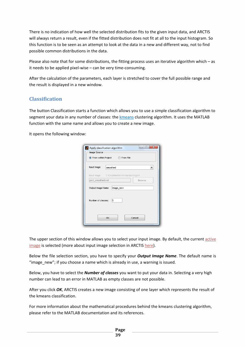
Classification
The button Classification starts a function which allows you to use a simple classification algorithm to
segment your data in any number of classes: the kmeans clustering algorithm. It uses the MATLAB
function with the same name and allows you to create a new image.
It opens the following window:
The upper section of this window allows you to select your input image. By default, the current active
image is selected (more about input image selection in ARCTIS here).
Below the file selection section, you have to specify your Output Image Name. The default name is
“image_new”; if you choose a name which is already in use, a warning is issued.
Below, you have to select the Number of classes you want to put your data in. Selecting a very high
number can lead to an error in MATLAB as empty classes are not possible.
After you click OK, ARCTIS creates a new image consisting of one layer which represents the result of
the kmeans classification.
For more information about the mathematical procedures behind the kmeans clustering algorithm,
please refer to the MATLAB documentation and its references.
Page40
FunctionReference:ViewingImages
ActiveImage,DisplayMethodandBandSelection
In the uppermost part of the View section, the popup menu for selecting the active image is
displayed. Below, ARCTIS displays another popup menu labeled Display Method. There you can
switch between two options: RGB view and single band view.
Depending on the display method you choose, ARCTIS displays either three popup menus for
selecting bands for the red, green and blue channel (RGB view) or one popup menu for selecting a
band to display and a second one for choosing your desired colormap.
TheViewButton
This button displays the active image using the current contrast enhancement settings. Each click on
this button results in a new window, regardless of the number of the currently open windows – you
can have as many as you want.
ContrastOptions
The values of images in ARCTIS might range – depending on the format –from 0 to 255 (uint8) or
from 0 to 65535 (uint16). Depending on your data source, type and preprocessing steps, your image
data might vary in a much smaller range, so if ARCTIS would display the data as if the values
mentioned above were the highest and lowest, you are likely to not see anything. This being the
case, ARCTIS offers various possibilities to enhance the contrast of your image and to “stretch” the
data to cover a wider range.
By default, ARCTIS enables contrast stretching; if you want to display the original data, just disable
the Enhance Contrast checkbox.
The difference to the contrast functions from the preprocessing section mentioned above is that
ARCTIS does not really alter the data, it just changes the way the data is displayed.
ARCTIS offers several contrast enhancing methods/algorithms; you can select them using the Options
button:
Page41
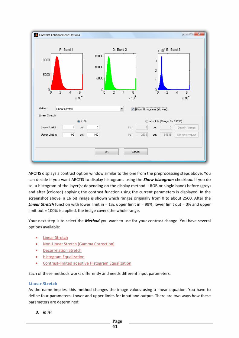
ARCTIS displays a contrast option window similar to the one from the preprocessing steps above: You
can decide if you want ARCTIS to display histograms using the Show histogram checkbox. If you do
so, a histogram of the layer(s; depending on the display method – RGB or single band) before (grey)
and after (colored) applying the contrast function using the current parameters is displayed. In the
screenshot above, a 16 bit image is shown which ranges originally from 0 to about 2500. After the
Linear Stretch function with lower limit in = 1%, upper limit in = 99%, lower limit out = 0% and upper
limit out = 100% is applied, the image covers the whole range.
Your next step is to select the Method you want to use for your contrast change. You have several
options available:
Linear Stretch
Non‐Linear Stretch (Gamma Correction)
Decorrelation Stretch
Histogram Equalization
Contrast‐limited adaptive Histogram Equalization
Each of these methods works differently and needs different input parameters.
LinearStretchAs the name implies, this method changes the image values using a linear equation. You have to
define four parameters: Lower and upper limits for input and output. There are two ways how these
parameters are determined:
3. in %:

Page42
You can define the input and output limits as a fractile in percent. Note that while output
limits stay the same for each layer and are only determined by the data type (see here; if you
set the output limit to 50% and are using 16 bit images which range from 0 to 65535, ARCTIS
calculates 50% = 32768), the input limits vary from layer to layer as they are determined by
the layer histogram.
The advantage of the percentage input is that you obtain an image which uses the same
value range in each layer. But, of course, dependencies between the layers are removed,
especially if the value range of the input layers varies widely. So if you want to keep the
correct relationship between the layers, it is recommended to use the second way of
determining input and output limits:
4. absolute values:
You also can define the input and output limit values directly using the absolute method. This
method applies the same formula to all layers, so the relationship between the layers is kept.
You have the possibility to automatically obtain the minimum and maximum values of your
whole image (not layer!) by clicking the correspondent buttons. If you use these values, the
resulting image covers the whole range (depending on the data type); if your image has 16
bit, the lowest value of all layers will be 0 and the highest 65535.
ARCTIS now calculates the output values applying the linear equation
∗
to each pixel where
inij = input pixel values outij = output pixel values lin = lower limit in for the current layer uin = upper limit in for the current layer lout = lower limit out for the current layer uout = upper limit out for the current layer.
Non‐LinearStretch(GammaCorrection)This method is similar to the linear stretch method, the only difference is an additional fifth
parameter, called Gamma. The other four parameters (lower and upper limits for input and output)
are the same and are entered in the same way as written above. The above mentioned equation
changes to the non‐linear equation
∗
where
inij = input values outij = output values γ = Gamma lin = lower limit in uin = upper limit in
Page43
lout = lower limit out uout = upper limit out.
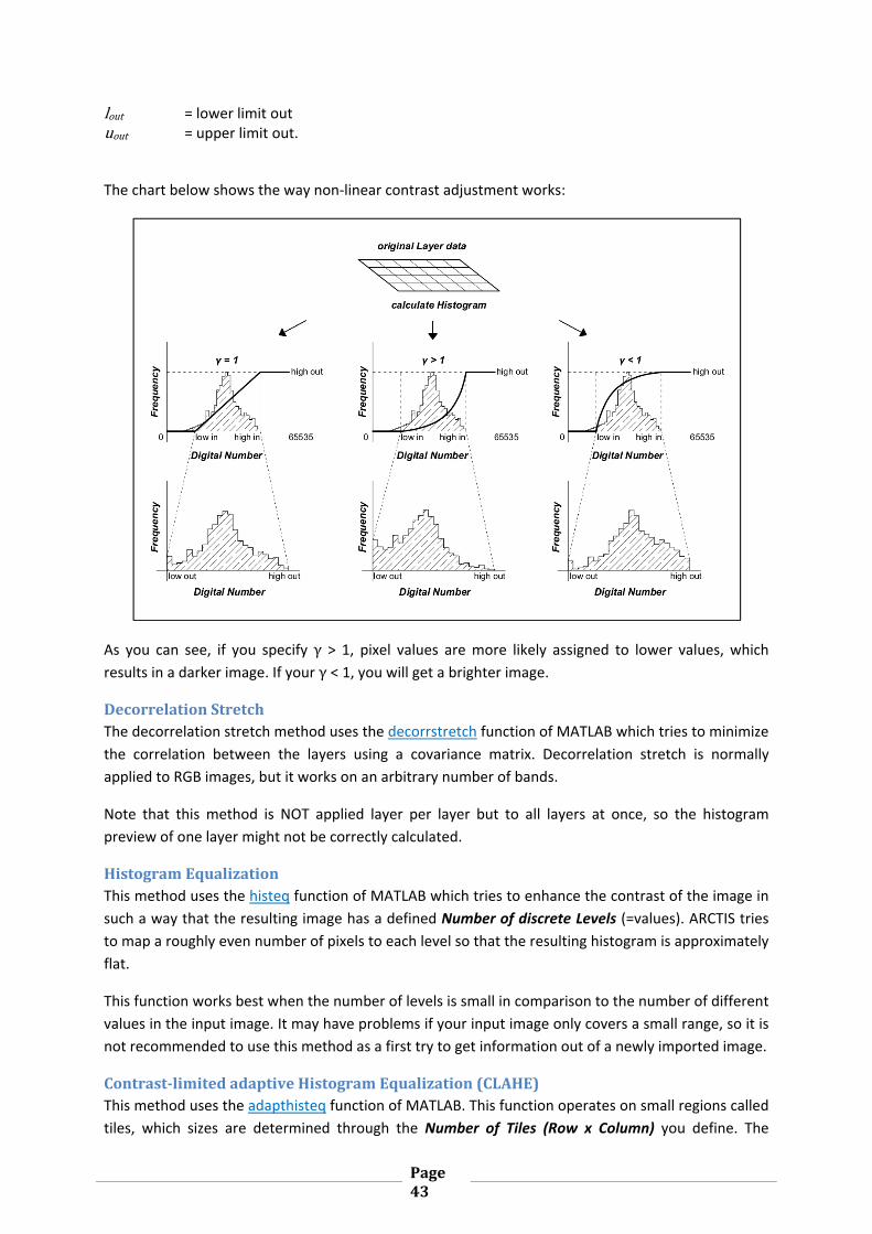
The chart below shows the way non‐linear contrast adjustment works:
As you can see, if you specify γ > 1, pixel values are more likely assigned to lower values, which
results in a darker image. If your γ < 1, you will get a brighter image.
DecorrelationStretchThe decorrelation stretch method uses the decorrstretch function of MATLAB which tries to minimize
the correlation between the layers using a covariance matrix. Decorrelation stretch is normally
applied to RGB images, but it works on an arbitrary number of bands.
Note that this method is NOT applied layer per layer but to all layers at once, so the histogram
preview of one layer might not be correctly calculated.
HistogramEqualizationThis method uses the histeq function of MATLAB which tries to enhance the contrast of the image in
such a way that the resulting image has a defined Number of discrete Levels (=values). ARCTIS tries
to map a roughly even number of pixels to each level so that the resulting histogram is approximately
flat.
This function works best when the number of levels is small in comparison to the number of different
values in the input image. It may have problems if your input image only covers a small range, so it is
not recommended to use this method as a first try to get information out of a newly imported image.
Contrast‐limitedadaptiveHistogramEqualization(CLAHE)This method uses the adapthisteq function of MATLAB. This function operates on small regions called
tiles, which sizes are determined through the Number of Tiles (Row x Column) you define. The
Page44
contrast of each tile is enhanced in a way that it fits the specified Distribution: uniform results in a
flat histogram, rayleigh in a Bell‐shaped curve and exponential in a curved histogram. The
neighboring tiles are then combined using bilinear interpolation to eliminate artificially induced
boundaries.
Other parameters you can define are
Clip Limit: This number specifies a limit for contrast enhancement. It ranges from 0 to 1;
higher numbers result in more contrast.
Number of Bins: This value specifies the number of bins used during histogram calculation.
Higher values result in greater dynamic range but in slower processing speed.
Range: You can specify if your output image should cover the full possible range (0…65535 if
you are working on a 16 bit image) or if ARCTIS should keep the range of the original image.
Alpha (only used when Distribution is set to rayleigh or exponential): Distribution parameter
If you have entered your contrast enhancement settings, save them by clicking OK. Pressing OK again
on the Apply Contrast Functions to Image window starts the process. If the calculation is finished,
ARCTIS displays your newly created image using the best triple algorithm.
TrueColor,FalseColorIR
These functions preselect certain band combinations depending on the wavelengths of each band.
They are only available if wavelength information is available to ARCTIS ‐ see here.
ARCTIS looks for the wavelengths closest to the values
Blue: 470 nanometers
Green: 540 nanometers
Red: 650 nanometers
NIR: 800 nanometers
and then selects the bands found in the band selection popup menus. Be careful: even if the
wavelengths of your data are far away from the values above, ARCTIS will always find suitable bands
as it just takes the bands with wavelengths nearest to those values.
SaveAs
This button allows you to export your active image as it would display in ARCTIS using the current
contrast enhancement settings. It makes no difference if you already clicked the View! button to
display it; ARCTIS just calculates how the image would look like and allows you to save it as a JPG or
JPG2000 file.
Please note that ARCTIS saves only the currently selected bands, so it differs from the export function
above.

Page45
FunctionReference:OtherTools
Animation
This tool allows you to display and export animated images of your dataset. If you click the button,
ARCTIS shows the active image in a new window and also displays the animation control window:
In this window, you can change the Speed of the animation using either the slider or enter the
desired value directly. In ARCTIS, you specify the animation speed in seconds per band, so the value
defines how long a single band/band combination is displayed.
You are also able to jump to any band you want using either the Current Band slider or you can enter
the desired band number directly. Also you can change the Colormap you want to use when
displaying an image.
Below, you can select the way ARCTIS displays the animation. There are several possibilities:
OriginalDataIf you select this option, ARCTIS displays each band as it is. Nevertheless, if the Enhance Contrast
checkbox is checked, ARCTIS applies the currently selected contrast enhancement algorithm with the
current parameters to the each band before displaying it.
Differencevs.NextBandIf you select this option, ARCTIS calculates the difference between the current and the next band and
displays the result using the selected colormap. If the Enhance Contrast checkbox is checked, ARCTIS
applies the currently selected contrast enhancement algorithm with the current parameters to the
each band before displaying it.
Page46
When ARCTIS reaches the last layer, it continues with the first one again. This may result in
unexpected results, as one “animation slide” is the calculated difference between the first and the
last layer.
Differencevs.NextBand(absolutevalues)If you select this option, ARCTIS calculates the difference between the current and the next band,
convert the values to absolute values and displays the result using the selected colormap. This option
differs from the one above in the way that ARCTIS does not distinguish positive or negative
differences; just the absolute values of the differences are displayed. If the Enhance Contrast
checkbox is checked, ARCTIS applies the currently selected contrast enhancement algorithm with the
current parameters to the each band before displaying it.
When ARCTIS reaches the last layer, it continues with the first one again. This may result in
unexpected results, as one “animation slide” is the calculated difference between the first and the
last layer.
3BandsasRGB(1/2/3,2/3/4,3/4/5)If you select this option, ARCTIS displays three bands as an RGB image before. The first image of your
animation consists of band 1 shown in the red, 2 in the green and 3 in the blue channel. The second
image shows band 2 in the red, 3 in the green and 4 in the blue channel and so on. The resulting
image has as many layers as the original one, as each layer is used three times.
If the Enhance Contrast checkbox is checked, ARCTIS applies the currently selected contrast
enhancement algorithm with the current parameters to the each band before displaying it.
When ARCTIS reaches the last layer, it continues with the first one again.
3BandsasRGB(1/2/3,3/4/5,6/7/8)If you select this option, ARCTIS displays three bands as an RGB image before. The first image of your
animation consists of band 1 shown in the red, 2 in the green and 3 in the blue channel. The second
image shows band 4 in the red, 5 in the green and 6 in the blue channel and so on. The resulting
image only one third of the layers as the original one, as each layer is only used once.
If the Enhance Contrast checkbox is checked, ARCTIS applies the currently selected contrast
enhancement algorithm with the current parameters to the each band before displaying it.
When ARCTIS reaches the last layer, it continues with the first one again.
Below, there are buttons to Start and Stop your animation; while it is running, the Current Band
slider is disabled.
There is also the possibility to Export your current animation as an animated GIF image, AVI movie
file or Motion JPEG movie. Please note that MATLAB does not support the creation of 16bit‐GIF or
AVI files. If you try to export a 16bit image to AVI or GIF, a warning is issued and the animation is
converted to 8bit.
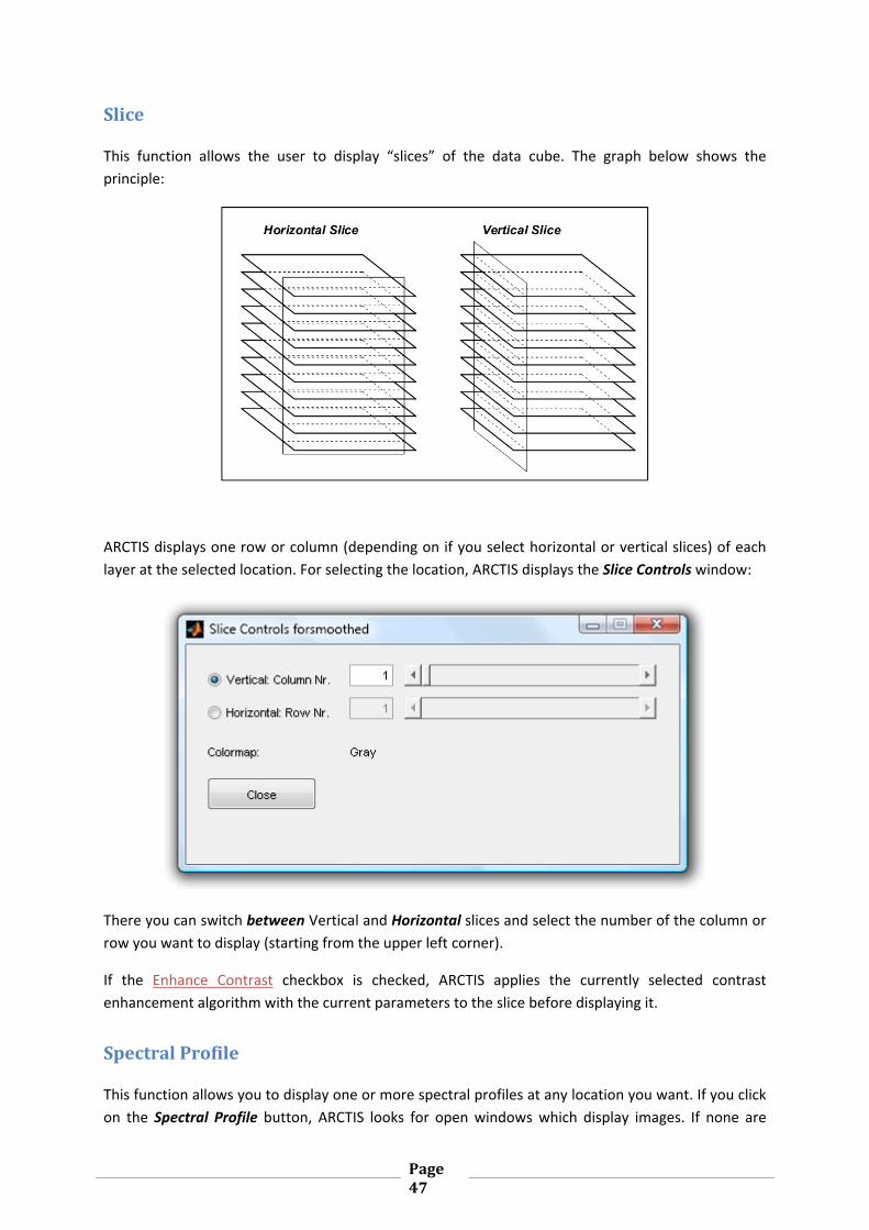
Page47
Slice
This function allows the user to display “slices” of the data cube. The graph below shows the
principle:
ARCTIS displays one row or column (depending on if you select horizontal or vertical slices) of each
layer at the selected location. For selecting the location, ARCTIS displays the Slice Controls window:
There you can switch between Vertical and Horizontal slices and select the number of the column or
row you want to display (starting from the upper left corner).
If the Enhance Contrast checkbox is checked, ARCTIS applies the currently selected contrast
enhancement algorithm with the current parameters to the slice before displaying it.
SpectralProfile
This function allows you to display one or more spectral profiles at any location you want. If you click
on the Spectral Profile button, ARCTIS looks for open windows which display images. If none are
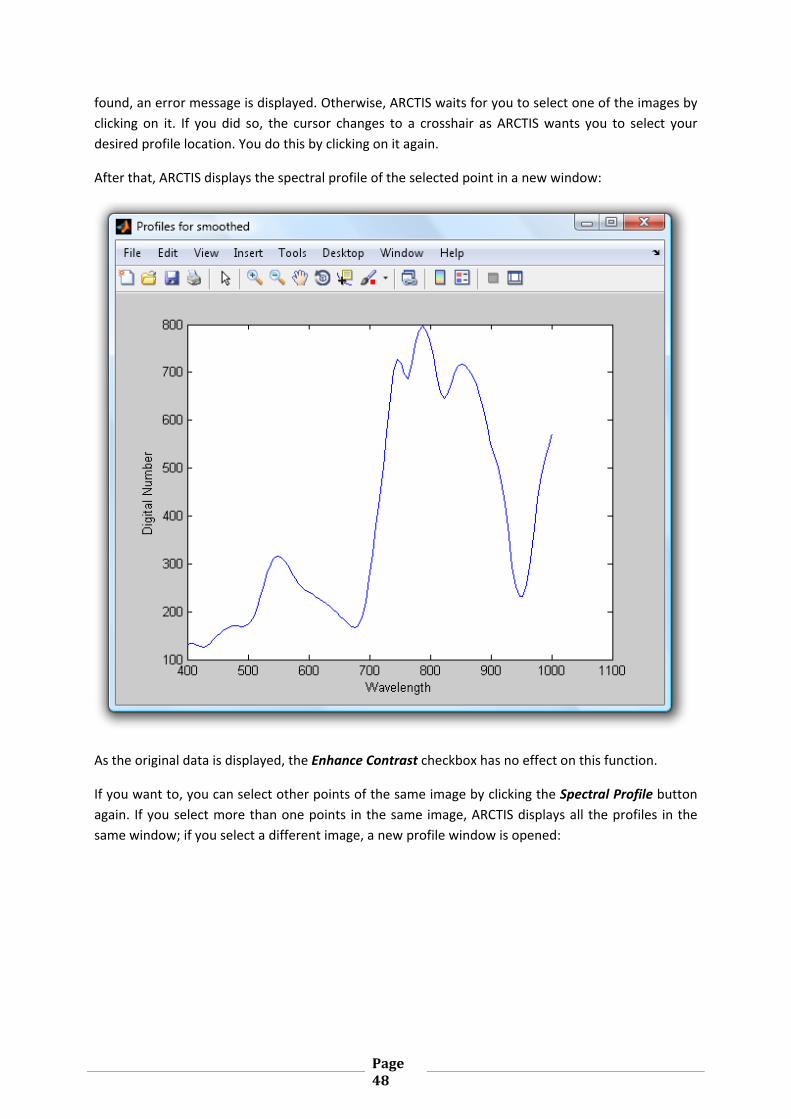
Page48
found, an error message is displayed. Otherwise, ARCTIS waits for you to select one of the images by
clicking on it. If you did so, the cursor changes to a crosshair as ARCTIS wants you to select your
desired profile location. You do this by clicking on it again.
After that, ARCTIS displays the spectral profile of the selected point in a new window:
As the original data is displayed, the Enhance Contrast checkbox has no effect on this function.
If you want to, you can select other points of the same image by clicking the Spectral Profile button
again. If you select more than one points in the same image, ARCTIS displays all the profiles in the
same window; if you select a different image, a new profile window is opened:
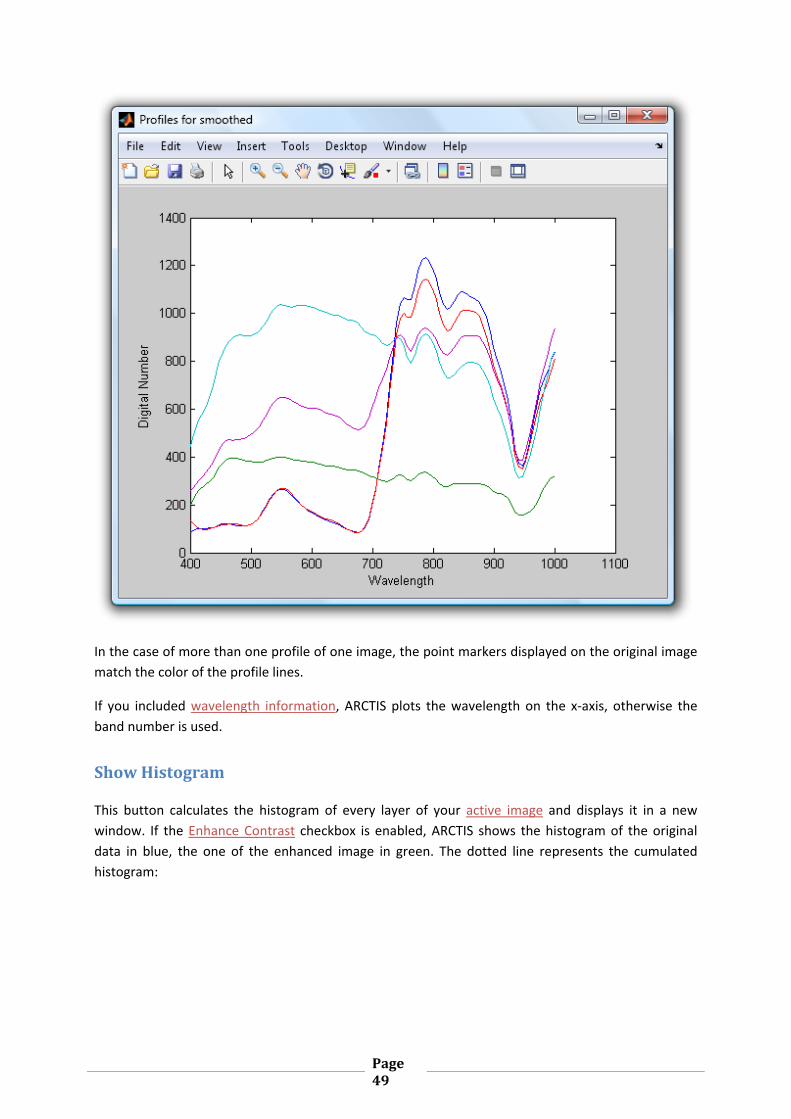
Page49
In the case of more than one profile of one image, the point markers displayed on the original image
match the color of the profile lines.
If you included wavelength information, ARCTIS plots the wavelength on the x‐axis, otherwise the
band number is used.
ShowHistogram
This button calculates the histogram of every layer of your active image and displays it in a new
window. If the Enhance Contrast checkbox is enabled, ARCTIS shows the histogram of the original
data in blue, the one of the enhanced image in green. The dotted line represents the cumulated
histogram:
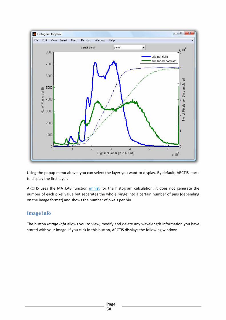
Page50
Using the popup menu above, you can select the layer you want to display. By default, ARCTIS starts
to display the first layer.
ARCTIS uses the MATLAB function imhist for the histogram calculation; it does not generate the
number of each pixel value but separates the whole range into a certain number of pins (depending
on the image format) and shows the number of pixels per bin.
Imageinfo
The button Image Info allows you to view, modify and delete any wavelength information you have
stored with your image. If you click in this button, ARCTIS displays the following window:
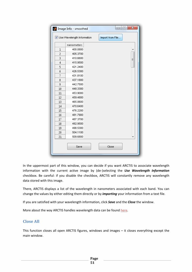
Page51
In the uppermost part of this window, you can decide if you want ARCTIS to associate wavelength
information with the current active image by (de‐)selecting the Use Wavelength Information
checkbox. Be careful: if you disable the checkbox, ARCTIS will constantly remove any wavelength
data stored with this image.
There, ARCTIS displays a list of the wavelength in nanometers associated with each band. You can
change the values by either editing them directly or by importing your information from a text file.
If you are satisfied with your wavelength information, click Save and the Close the window.
More about the way ARCTIS handles wavelength data can be found here.
CloseAll
This function closes all open ARCTIS figures, windows and images – it closes everything except the
main window.
Page52
Zoom2Cursor
This function allows you to interactively zoom to the cursor location. If you start this function, ARCTIS
looks for open windows which display images. If none are found, an error message is displayed.
Otherwise, ARCTIS waits for you to select one of the images by clicking on it. The cursor then changes
to a crosshair and ARCTIS zooms the image to the cursor location.
Clicking the left mouse button increases the magnification, clicking the right decreases it. A double
click on any mouse button resets the zoom to the original size.
If you want to close the function, just click the little X in the lower left corner of the window.
Stretch2Cursor
This function allows you to display the area around the cursor stretched from 5% to 95%. You can use
it to analyze every part of your image in detail. If you move the cursor around on your image, ARCTIS
calculates the stretched subimage on time and displays it at the cursor location.
If you start this function, ARCTIS looks for open windows which display images. If none are found, an
error message is displayed. Otherwise, ARCTIS waits for you to select one of the images by clicking on
it. The cursor then changes to a crosshair and ARCTIS displays the small overlay image. By default, its
size is 200 by 200 pixels, but you can change the size using the scroll wheel; double clicking any
mouse button resets the size to its default.
If you want to close the function, just click the little red X in the lower left corner of the window.

Page53
Appendix
DataTypes
In ARCTIS, images typically have two data types: 8 or 16 bit unsigned integer. Consequently, image
values reach any non‐negative integer between 0 and 255 (8 bit) or 0 and 65535 (16 bit).
During calculations, it is often necessary to convert the image values into other data types, but the
output images are always converted back to the input format before saving.
Although we tried to avoid this effect, it sometimes may occur that during one or the other
calculation, a result may reach an out‐of‐bounds‐value. In these cases, the result is set to either 0,
255 or 65535 automatically.
ImageStretching
ARCTIS is mainly a tool for displaying data. Therefore, after many operations, ARCTIS automatically
adjusts the result in order to make it cover the whole possible range. Nevertheless, it is still possible
to get ones hands on the original results where it is reasonable:
ARCTIS stores two parameters in the ImageInfo Variable called ImageInfo.Param1 and
Imageinfo.Param2. To see the original results you just need to apply the following calculation in
MATLAB:
∗ 1 2
SelectingFilesinARCTIS
ARCTIS generally allows you to select every file you want as input data during most image processing
operations (just select the From File radio button and use the Browse… button for file selection). Of
course, the input files have to be ARCTIS images and should have the same size and geographic
location as the ones already existing in your project. So it is recommended to import every image
using the import function before applying any image processing operations to it.
WorldFiles
ARCTIS is able to read world files for obtaining georeferencing information. A world file is a plain text
file consisting of 6 lines (WIKIPEDIA, 2012):
Line 1: A: pixel size in the x‐direction in map units/pixel
Line 2: D: rotation about y‐axis
Line 3: B: rotation about x‐axis
Line 4: E: pixel size in the y‐direction in map units, almost always negative[3]
Line 5: C: x‐coordinate of the center of the upper left pixel
Line 6: F: y‐coordinate of the center of the upper left pixel.

Page54
ARCTIS generally uses the extension “.tfw” for world files and names them after the raster image
they belong to.
PointSelectioninARCTIS
Point selection in ARCTIS typically consists of two steps. First, you have to select the image you want
to select a point in by clicking on it once with the left mouse button. After that, your cursor turns into
a crosshair and allows you to select the point you want by clicking on it a second time.
For many operations, it is not important on which image you click as the image is only needed to get
the location information. However, you may experience some problems if you have images of
different projects open at the same time or if your images in one project have different sizes, which
is not recommended.
PolygonSelectioninARCTIS
Polygon Selection in ARCTIS typically consists of three steps. First, you have to select the image you
want to select a point in by clicking on it once with the left mouse button. After that, your cursor
turns into a crosshair and you can draw the vertexes of your polygon by single‐clicking with the left
mouse button. If you want to close your polygon, you can either double click anywhere or click the
starting vertex of your polygon again. You now have the possibility to move your polygon around
using drag&drop or you can move single vertexes in the same way. As a third step, if you are satisfied
with your polygon, double‐click it. It now turns red and your polygon has been selected.
Note: It may sometimes take some time for ARCTIS to process your clicks and actions during polygon
selection, so wait a little after each click in order to wait for ARCTIS to process your actions.
NoData‐Values
ARCTIS offers very limited support of NoData values. It does this via calculating a mask which
identifies each data point as “Data” or “NoData”. NoData‐Values are set during the import process,
ant cannot be changed afterwards.
ARCTIS ignores NoData‐Values only for the contrast enhancement operations; for every other image
processing operation, these values are treated as normal values. Therefore it is recommended to use
only images without any missing data for the analysis in ARCTIS.
ColormapsandIndexedData
Generally, there are two types of images in MATLAB: RGB images consisting of three bands
representing the red, green and blue spectra, and indexed images, consisting of one layer and a
colormap.
Consequently, you can decide if you want to display three bands of your data as an RGB composite
image, or just one layer using a colormap.
Page55
A colormap just tells ARCTIS which color to assign to which value. The number of different colors in a
colormap depends on the data type of your image: if you use 16bit images, the colormap needs to
have 65536 different entries as this is the number possible values of your image; for 8bit, the number
is 256.
ARCTIS offers several different colormaps predefined in MATLAB. For more information, please refer
to the MATLAB command colormap.
WavelengthInformation
ARCTIS offers the possibility to associate wavelength information with each image. This is done either
by importing a text file or by reading it from an ENVI header file. In ARCTIS, the way wavelength info
is stored is simple: For each band of your image, a corresponding wavelength is saved. ARCTIS then
simply treats each band as if it covers exactly this wavelength.
It is important that you use nanometers for the wavelength unit in order to use the functions True
Color and False Color IR because they are looking for certain wavelengths predefined in this unit.
TheBest‐TripleAlgorithm
This algorithm is used to preselect a band combination which allows you to get as much information
as possible out of a newly created image. It first generates a correlation matrix out of the whole
image and locates the two least correlated bands. Then it looks which band has the least correlation
to these two bands and takes it as the third band.
Results may vary because due to memory reasons, ARCTIS does not take the whole image but only a
random sample for the generation of the correlation matrix. But as stated above, this algorithm is
only used to give you a quick overview of your newly created image, and you can select any band
combination you want for further analysis.
References
MATLAB Documentation Center v2012b, http://www.mathworks.com/help/, October 2012
Garcia, D., 2009. Robust smoothing of gridded data in one and higher dimensions with missing
values. Computational Statistics and Data Analysis 54, 1167‐1178
Eilers, P.H., 2003. A perfect smoother. Anal. Chem. 75, 3631‐3636.
Khanna, S., Palacios‐Orueta, A., Whiting, M.L., Ustin, S.L.,Riaño, D., Litago, J., 2007. Development of
angle indexes for soil moisture estimation, dry matter detection and land‐cover discrimination.
Remote Sensing of Environment 109 (2) , 154‐165.
Pearson, K., 1901. On Lines and Planes of Closest Fit to Systems of Points in Space. Philosophical
Magazine 2 (6), 559–572.
Roberts, L., 1963. Machine Perception Of Three‐Dimensional Solids. Lincoln Laboratory, TR 315.

Page56
Whittaker, E.T., 1923. On a new method of graduation. Proceedings of the Edinburgh Mathematical
Society 41, 62‐75