for managers and entrepreneurs

Accounting and Finance

for Managers and Entrepreneurs

Publication Date: August 2021

Accounting and Finance for Managers and Entrepreneurs

Copyright © 2021 by

DELTACPE LLC

All rights reserved. No part of this course may be reproduced in any form or by any means, without permission in

writing from the publisher.

The author is not engaged by this text or any accompanying lecture or electronic media in the rendering of legal,

tax, accounting, or similar professional services. While the legal, tax, and accounting issues discussed in this

material have been reviewed with sources believed to be reliable, concepts discussed can be affected by changes

in the law or in the interpretation of such laws since this text was printed. For that reason, the accuracy and

completeness of this information and the author's opinions based thereon cannot be guaranteed. In addition,

state or local tax laws and procedural rules may have a material impact on the general discussion. As a result, the

strategies suggested may not be suitable for every individual. Before taking any action, all references and citations

should be checked and updated accordingly.

This publication is designed to provide accurate and authoritative information in regard to the subject matter

covered. It is sold with the understanding that the publisher is not engaged in rendering legal, accounting, or other

professional service. If legal advice or other expert advice is required, the services of a competent professional

person should be sought.

—-From a Declaration of Principles jointly adopted by a committee of the American Bar Association and a

Committee of Publishers and Associations.

All numerical values in this course are examples subject to change. The current values may vary and may not be

valid in the present economic environment.

Course Description

This course covers everything businesspeople and managers need to know about accounting and finance. It is

directed toward the businessperson who must have financial and accounting knowledge but has little formal

training in finance or accounting. This could include a newly promoted middle manager or a marketing manager

of a small company. The entrepreneur or sole proprietor also needs this knowledge; he or she may have brilliant

product ideas, but not the limited ideas about financing. The goal of the course is to provide a working knowledge

of the fundamentals of finance and accounting that can be applied, regardless of the firm size, in the real world.

It gives managers the understanding they need to function effectively with their colleagues in finance.

Field of Study Accounting

Level of Knowledge Basic to Intermediate

Prerequisite Basic Math and Accounting

Advanced Preparation None

i

Table of Contents

Preface ..................................................................................................................................................................... viii

Chapter 1: Essentials of Accounting and Finance ....................................................................................................1

Learning Objectives ................................................................................................................................................1

The Significance of Finance ....................................................................................................................................1

The Scope of Finance .............................................................................................................................................3

The Relationship Between Accounting and Finance ..............................................................................................4

Management Responsibilities ................................................................................................................................6

Financial and Operating Environment ...................................................................................................................9

Conclusion ........................................................................................................................................................... 13

Chapter 1 Review Questions ............................................................................................................................... 14

Chapter 2: Types of Cost Data and Cost Analysis ................................................................................................. 15

Learning Objectives ............................................................................................................................................. 15

The Purposes of Cost Data .................................................................................................................................. 15

Types of Costs ..................................................................................................................................................... 16

Cost Analysis........................................................................................................................................................ 21

Conclusion ........................................................................................................................................................... 22


Chapter 3: Contribution Analysis .......................................................................................................................... 25


Contribution Margin Analysis .............................................................................................................................. 25

Bid Price Determination ...................................................................................................................................... 30

Conclusion ........................................................................................................................................................... 31


Chapter 4: Break-Even and Cost-Volume-Profit Analysis ..................................................................................... 33


ii

Cost-Volume-Profit Analysis................................................................................................................................ 33

Break-Even Analysis ............................................................................................................................................ 34

Margin of Safety .................................................................................................................................................. 38

Cash Break-Even Point ........................................................................................................................................ 38

Operating Leverage ............................................................................................................................................. 39

Sales Mix Analysis ............................................................................................................................................... 41

Conclusion ........................................................................................................................................................... 42


Chapter 5: Cost Data Analysis ............................................................................................................................... 44


The Concept of Relevant Costs ........................................................................................................................... 44

Special Orders vs. Standard Products ................................................................................................................. 46

Make-or-Buy Decision ......................................................................................................................................... 48

Sell or Process Further ........................................................................................................................................ 49

Add or Drop a Product Line ................................................................................................................................. 50

Constraining Factors ........................................................................................................................................... 51

Conclusion ........................................................................................................................................................... 52


Chapter 6: Financial Forecasting and Budget Planning ....................................................................................... 54


Benefits of Forecasting ........................................................................................................................................ 54

The Financial Forecasting Process ....................................................................................................................... 56

The Budgetary Process ........................................................................................................................................ 59

The Operational Budget ...................................................................................................................................... 63

The Financial Budget ........................................................................................................................................... 69

Other Considerations .......................................................................................................................................... 72

Conclusion ........................................................................................................................................................... 72

iii


Chapter 7: Cost Control and Variance Analysis .................................................................................................... 74


Benefits of Variance Analysis .............................................................................................................................. 75

Setting Standards ................................................................................................................................................ 76

Analyzing Variances............................................................................................................................................. 77

Static vs. Flexible Budgeting ................................................................................................................................ 84

Other Considerations .......................................................................................................................................... 86

Conclusion ........................................................................................................................................................... 89


Chapter 8: Financial Assets ................................................................................................................................... 92


The Concept of Working Capital ......................................................................................................................... 92

Cash Management .............................................................................................................................................. 93

Other Considerations ........................................................................................................................................ 100

Conclusion ......................................................................................................................................................... 102

Chapter 8 Review Questions ............................................................................................................................. 103

Chapter 9: Accounts Receivable and Credit........................................................................................................ 105

Learning Objectives ........................................................................................................................................... 105

Implementing Credit System ............................................................................................................................. 105

Establishing Credit and Collection Policies ........................................................................................................ 106

Optimizing Accounts Receivable ....................................................................................................................... 108

Conclusion ......................................................................................................................................................... 112

Chapter 9 Review Questions ............................................................................................................................. 113

Chapter 10: Inventory ......................................................................................................................................... 114


Inventory Management .................................................................................................................................... 114

iv

Economic Order Quantity ................................................................................................................................. 118

Conclusion ......................................................................................................................................................... 123

Chapter 10 Review Questions ........................................................................................................................... 124

Chapter 11: Time Value of Money ...................................................................................................................... 125


Future Values: How Money Grows ................................................................................................................... 125

Present Value: How Much Future Money is Worth Now ................................................................................. 129

Applications ....................................................................................................................................................... 131

Conclusion ......................................................................................................................................................... 137


Chapter 12: Capital Investment Decisions .......................................................................................................... 143


Investment Analysis Techniques ....................................................................................................................... 144

The Effect of Income Taxes ............................................................................................................................... 149

Depreciation Methods ...................................................................................................................................... 151

The Cost of Capital ............................................................................................................................................ 156

Conclusion ......................................................................................................................................................... 158


Chapter 13: Managerial Performance Measures ............................................................................................... 160


What is Return on Investment .......................................................................................................................... 160

Profit Planning ................................................................................................................................................... 163

Return on Equity ............................................................................................................................................... 165

Conclusion ......................................................................................................................................................... 169


Chapter 14: Segmental Performance Measures ................................................................................................. 171


v

Use of Segmental Analysis ................................................................................................................................ 171

Responsibility Centers ....................................................................................................................................... 172

Transfer Pricing ................................................................................................................................................. 184

Conclusion ......................................................................................................................................................... 187


Chapter 15: Short-Term Financing Options ........................................................................................................ 190


Definition and Considerations........................................................................................................................... 190

Sources .............................................................................................................................................................. 193

Commercial Paper ............................................................................................................................................. 199

Receivable Financing ......................................................................................................................................... 199

Inventory Financing ........................................................................................................................................... 201

Other Considerations ........................................................................................................................................ 203

Conclusion ......................................................................................................................................................... 204


Chapter 16: Intermediate-Term Financing ......................................................................................................... 206


Major Forms ...................................................................................................................................................... 206

Conclusion ......................................................................................................................................................... 211


Chapter 17: Long-Term Debt and Equity Financing ............................................................................................ 213


The Role of Investment Bankers ....................................................................................................................... 214

Publicly vs. Privately Placed Securities .............................................................................................................. 215

Public Issuance .................................................................................................................................................. 216

Venture Capital Financing ................................................................................................................................. 222

Sources of Long-Term Debt Financing .............................................................................................................. 223

vi

Equity Securities ................................................................................................................................................ 230

Other Consideration .......................................................................................................................................... 237

Conclusion ......................................................................................................................................................... 240


Chapter 18: Uses of Financial Statements .......................................................................................................... 243


Balance Sheet .................................................................................................................................................... 244

Income Statement ............................................................................................................................................. 247

Statement of Cash Flows ................................................................................................................................... 248

Conclusion ......................................................................................................................................................... 254


Chapter 19: Accounting Conventions and Recording Financial Data ................................................................. 256


The Accounting Equation .................................................................................................................................. 256

The Account, Ledger, and Chart of Accounts .................................................................................................... 261

Steps in Recording Transactions ....................................................................................................................... 263

Conclusion ......................................................................................................................................................... 264


Chapter 20: Financial Health and Fitness ........................................................................................................... 266


Purposes of the Financial Statements ............................................................................................................... 267

Comparative Financial Statements ................................................................................................................... 267

Ratio Analysis .................................................................................................................................................... 271

Conclusion ......................................................................................................................................................... 283


Glossary ................................................................................................................................................................. 286

Index ...................................................................................................................................................................... 296

vii

Review Question Answers ..................................................................................................................................... 298

viii

Preface

This course is directed toward the businessperson who must have financial and accounting knowledge but has not

had formal training in finance or accounting - perhaps a newly promoted middle manager or a marketing manager

of a small company who must know some basic finance concepts. The entrepreneur or sole proprietor also needs

this knowledge; he or she may have brilliant product ideas, but not the slightest idea about financing.

The goal of the course is to provide a working knowledge of the fundamentals of finance and accounting that can

be applied, regardless of the firm size, in the real world. It gives non-financial managers the understanding they

need to function effectively with their colleagues in finance.

We show you the strategies for evaluating investment decisions such as return on investment analysis. You will

see what you need to know, what to ask, which tools are important, what to look for, what to do, how to do it,

and what to watch out for. You will find the course easy to read and useful. Many practical examples, illustrations,

guidelines, measures, rules of thumb, graphs, diagrams, and tables are provided to aid comprehension of the

subject matter.

You cannot avoid financial information. Profitability statements, rates of return, budgets, variances, asset

management, and project analyses, for example, are included in the non-financial manager's job.

The financial manager's prime functions are to plan for, obtain, and use funds to maximize the company's value.

The financial concepts, techniques, and approaches enumerated can also be used by any non-financial manager,

irrespective of his or her primary duties. All non-financial managers are in some way involved with the financial

areas of business.

This course is designed for non-financial executives in every functional area of responsibility in any type of

industry. Whether you are in marketing, manufacturing, personnel, operations research, economics, law,

behavioral sciences, computers, personal finance, taxes, or engineering, you must have a basic knowledge of

finance. Because your results will be measured in dollars and cents, you must understand the importance of these

numbers to optimize results in both the short and long term.

Knowledge of the content of this course will enable you to take on additional managerial responsibilities. You will

be better equipped to prepare, appraise, evaluate, and approve plans to accomplish departmental objectives. You

will be able to back up your recommendations with carefully prepared financial support as well as state your

particular measure of performance. By learning how to think in terms of finance and accounting, you can

intelligently express your ideas, whether they are based on marketing, production, personnel, or other concepts.

You will learn how to appraise where you have been, where you are, and where you are headed. Financial

measures show past, current, and future performance. Criteria are presented by which you can examine the

performance of your division and product lines and also formulate realistic profit goals.

Non-financial managers should have a grasp of financial topics, but may not need to calculate the mathematical

answer (e.g., discounted rate of return problem). Non-financial managers mainly need to know enough to ask

their financial colleagues what the discounted rate of return is for a variety of investment decisions. A decision

can then be based on their answer.

ix

You should have a basic understanding of financial information so as to evaluate the performance of your

responsibility center. Are things getting better or worse? What are the possible reasons? Who is responsible?

What can you do about it?

You need to know whether your business segment has adequate cash flow to meet requirements. Without

adequate funds, your chances of growth are restricted.

You must know what your costs are in order to establish a suitable selling price. What sales are necessary for you

to break even?

You may have to decide whether it is financially advantageous to accept an order at below the normal selling

price. If you have idle facilities, a lower price may still result in profitability.

You need to be able to express your budgetary needs in order to obtain proper funding for your department. You

may have to forecast future sales, cash flows, and costs to see if you will be operating effectively in the future.

Variance analysis helps you to spot areas of inefficiency or efficiency by comparing actual performance to

standards. What are the reasons that sales targets differ from actual sales? Why are costs much higher than

expected? The causes must be searched out so that corrective action may be taken.

You can undertake certain strategies to improve return on investment by enhancing profitability or using assets

more efficiently. You have to understand that money has associated with it a time value. Thus, you would prefer

projects that generate higher cash flows in earlier years. You may also want to compute growth rates.

You are often faced with a choice of alternative investment opportunities. You may have to decide whether to

buy machine A or machine B, whether to introduce a certain product line, or whether to expand.

In managing working capital, you have to get the most out of your cash, receivables, and inventory. How do you

get cash faster and delay cash payments? Don't forget that you need liquid funds to meet ongoing expenditures.

Should you extend credit to marginal customers? How much inventory should you order at one time? When

should you order the inventory?

In financing the business, a decision has to be made whether short-term, intermediate-term, or long-term

financing is suitable. The financing mix of the company in terms of equity or debt affects the cost of financing and

influences the firm's risk position. What is the best financing source in a given situation?

Taxes are important in any business decision; the after-tax effect is what counts. Proper tax planning will make

for wise decisions. Are you maximizing your allowable tax deductions?

Financial decisions are usually formulated on the basis of information generated by the accounting system of the firm.

Proper interpretation of the data requires an understanding of the assumptions and rules underlying such systems,

the convention adopted in recording information, and the limitations inherent in the information presented. To

facilitate this understanding, an understanding of basic accounting concepts and conventions is helpful. You should

be able to make an informed judgment on the financial position and operating performance of the entity. The balance

sheet, the income statement, and the statement of cash flows are the primary documents analyzed to determine the

company's financial condition. These financial statements are included in the annual report.

x

What has been the trend in profitability and return on investment? Will the business be able to pay its bills? How are

the receivables and the inventory turning over? Various financial statement analysis tools are useful in evaluating the

company's current and future financial conditions. These techniques include horizontal, vertical, and ratio analyses.

Keep this course handy for easy reference throughout your career; it will help you answer financial questions in

all the areas mentioned here and in any other matter involving money.

Field of Study Accounting Level of Knowledge Overview Prerequisite Basic Math Advanced Preparation None

1

Chapter 1: Essentials of Accounting and Finance

Learning Objectives

After studying this chapter, you will be able to:

• Identify the non-financial manager’s concern with financial planning

• Recognize the responsibilities of financial managers

• Distinguish between different business entities

A company exists to increase the wealth of its owners. Management is concerned with determining which

products and services are needed and putting them into the hands of its customers. Financial management deals

with planning decisions to achieve the goal of maximizing the owners' wealth. Because finance is involved in every

aspect of a company's operations, non-financial managers, like financial managers, cannot carry out their

responsibilities without accounting and financial information.

This chapter discusses the importance of finance, the scope and role of finance, and the language of finance. It

also addresses the relationship between accounting and finance, the responsibilities of management, and the

financial and operating environment in which finance is situated.

The Significance of Finance

You should have knowledge of finance and know how to apply it successfully in your particular departmental

functions. This is true whether you are a manager in production, marketing, personnel, operations, or any other

department. You should know what to look for, the right questions to ask, and where to get the answers. Financial

knowledge aids in planning, problem-solving, and decision making. Finance provides a road map in numbers and

analysis so that you can optimally perform your duties. Further, you must have financial and accounting

knowledge in order to understand the financial reports prepared by other segments of the organization. You must

know what the numbers mean even if you do not have to determine them.

Non-financial managers spend a good portion of their time planning. They set objectives and plan efficient courses

of action to obtain those objectives. There are many types of plans a non-financial manager might have to deal

2

with: production plans, financial plans, marketing plans, personnel plans, and so on. All of these plans are very

different, and all require some kind of financial knowledge.

Finance provides a link that facilitates communication among different departments. For example, the budget

communicates overall corporate goals to the department managers so they clearly know what is expected of

them; it also provides guidelines for how each department may conduct its activities. Most importantly you as a

department manager must present a strong case to upper management to justify budgetary allowances. You are

typically a participant providing input when the budget is prepared. You must identify any problems with the

proposed budget so they are rectified before the budget is finalized. Even after the budget is implemented, you

may suggest changes in subsequent budgetary formulations. Also, you must intelligently discuss the budget with

other organizational members. If you do not adequately understand the budget or communicate requirements

your department may fail to achieve its goals.

You have to formulate and provide upper management with documented information to obtain approval for

activities and projects (e.g., new product line). Your request for resources will entail financial plans for the

contemplated project. Here, a knowledge of forecasting and capital budgeting (selecting the most profitable of

several alternative long-term projects) is required. You may be involved in a decision of whether to lease or buy

an asset, such as equipment or an auto. Thus, you must consider the feasibility of the purchase. You must evaluate

and appraise monetary and manpower requests before submission. If you show signs of being ill-prepared, you

will give a negative impression that may result in the loss of resources.

In certain situations, you may obtain financial information about competitors. You should be able to understand

such information to make intelligent decisions. Because many of your decisions have financial implications, you

are continually interacting with financial managers. For instance:

1. Marketing decisions influence growth in sales and, as a result, there will be changes in plant and

equipment requirements that dictate increased external funding. Thus, the marketing manager must

have knowledge of the constraints of fund availability, inventory policies, and plant utilization.

2. The purchasing manager must know whether sufficient funds exist to take advantage of volume discounts.

The cost of raw materials is one of the most important manufacturing costs. The cost of alternative

materials along with their quality must be known since cost affects selling price, and inferior materials

may create production problems that eat into divisional profitability. Further, if materials are not

delivered on time, customer orders may not be filled in a timely fashion, thus adversely affecting future

sales.

3. Advertising managers also make key decisions related to finance. They can justify costs associated with

an advertising campaign by estimating its value. If customers want to buy your products, you have

something of value that will pay off in future earnings.

Capital investment projects (property, plant, and equipment) are closely tied to plans for product development,

marketing, and production. Thus, managers in these areas must be involved with planning and analyzing project

performance. As one non-financial manager I interviewed who was working for an electronics company said:

3

“My knowledge of accounting and finance helps me to report results, understand reports, control

expenses, allocate resources, budget for proper staffing, and decide the direction of my department. There

are thirty non-financial managers at my level within the company, and we work in a very competitive

environment as the company only promotes from within. Therefore, I need every edge I can get in order to

continue moving ahead, and my financial knowledge is a very important tool in my career development.”

For these reasons, as well as a host of others, you need basic financial knowledge to successfully conduct daily

activities.

You will learn in the following section the language of finance as well as the what and why. You will see the

responsibilities of financial managers, and the relationship between accounting and finance will be explained.

The Scope of Finance

Finance provides the discipline to all the components of the organization involved in decision making. Therefore,

you need knowledge of it to perform effectively. Knowledge of finance terminology, concepts, techniques, and

applications aids in the overall management of your departmental affairs.

For effective communication, you must be able not only to understand what financial people are saying but also

to express your ideas in their language. You can "open the door' to the finance department by having a better

understanding of the finance function and more productive working relationships with finance professionals.

If you master the finance vocabulary, you will be able to comprehend financial information (e.g., budgets), use

that information effectively, and communicate clearly about the quantitative aspects of performance and results.

You must clearly and thoughtfully express what you need to financial officers in order to perform effectively. To

do so, you have to be familiar with the basics of accounting, taxes, economics, and other aspects of finance.

Finance uses accounting information to make decisions regarding the receipt and use of funds to meet corporate

objectives. Accounting is generally broken down into two categories: financial accounting and managerial

accounting. Financial accounting records the financial history of the business and involves the preparation of

reports for use by external parties such as investors and creditors. Managerial accounting provides financial

information useful in making better decisions regarding the future. Financial and managerial accounting are

discussed later in this chapter. Chapter 18-21 covers financial accounting while chapters 2-7 and 13-14 zero in on

managerial accounting.

Finance involves many interrelated areas such as obtaining funds, using funds, and monitoring performance. It

enables you to look at current and prospective problems and find ways of solving them.

One important aspect of finance is the analysis of the return-risk tradeoff, which helps to determine if the

expected return is sufficient to justify the risks taken. The greater the risk with any decision (e.g., new product

line, new territory), the greater the return required. In managing your inventory of stock, for example, the less

4

inventory (merchandise held for resale) you keep, the higher the expected return (since less cash is tied up), but

also the greater the risk of running out of stock and thus losing sales and customer goodwill.

No matter who you are, you are involved with finance in one way or another. Financial knowledge is required of

marketing managers, production people, business managers, investment planners, economists, public relations

managers, operations research staff, lawyers, and tax experts, among others. For example, marketing managers

have to know product pricing and variance analysis. Financial managers must know how to manage assets so as

to optimize the rate of return. Production managers have to be familiar with budgeting and effective handling of

productive assets. Personnel executives must know about planning. Public relations managers must know about

the financial strengths of the business. Operations research staff has to know about the time value of money.

Investment planners have to be familiar with the valuation of stocks, bonds, and other investments.

The Relationship Between Accounting and Finance

Accounting is a necessary input and sub-function to finance. The primary distinctions between accounting and

finance relate to the treatment of funds and decision making. If you are employed by a large firm, the financial

responsibilities are probably carried out by the treasurer, controller, and financial vice president (chief financial

officer). The financial vice president is involved with financial policymaking and planning. He or she has financial

and managerial responsibilities, supervises all phases of financial activity, and serves as the financial adviser to

the board of directors. Management is involved with finance primarily in two ways. First, there is the record-

keeping, tracking, and controlling of the financial effects of prior and present operations, as well as obtaining

funds to satisfy current and future requirements. This function is of internal nature. The external function involves

outside entities.

Figure 1-1 shows an organization chart of the finance structure within a company.

5

Figure 1-1. Financial Activity Organization

Note that the controller and treasurer report to the vice president of finance. You should know the responsibilities

of these financial officers within your own organization and how the function of each affects you.The effective,

competent, and timely handling of controllership and treasurer functions will ensure corporate success. Table 1-

1 lists the typical responsibilities of the treasurer and controller, but there is no universally accepted precise

distinction between the two jobs. The functions may differ slightly between organizations because of personality

and company policy, but typically controllers are concerned with internal functions whereas treasurers are

responsible for external functions.

Table 1-1. Roles of Controller and Treasurer

Controller Treasurer

Accounting Obtaining Financing

Financial reporting Banking relationship

Custody of records Investment of funds

Interpretation of financial data Investor relations

Budgeting Cash management

Controlling operations Insure assets

Appraisal of results and making recommendations Fostering relationship with creditors and investors

Preparation of taxes Credit appraisal and collecting funds

Managing assets Deciding on the financing mix

Internal auditing Dividend disbursement

Protection of assets Pension management

Reporting to the government

Payroll

President (CEO)

Vice President Manufacturing

Vice President Finance (CFO)

Treasurer

Cash Manager Credit ManagerFinancial Planning Manager

Investment Manager

Controller

Tax ManagerCost Accounting

Manager

Vice President Marketing

6

The next section describes responsibilities of the financial manager, controller, and treasurer.

Management Responsibilities

Financial Manager

The financial manager plays an important role in the company's goals, policies, and financial success. The financial

manager's responsibilities include the following:

• Financial analysis and planning - determining the proper amount of funds to employ in the firm; that is,

designating the size of the firm and its rate of growth.

• Investment decisions - allocating funds to specific assets (things owned). The financial manager makes

decisions regarding the mix and type of assets acquired, as well as modification or replacement of assets.

• Financing and capital structure decisions - raising funds on favorable terms; that is, determining the nature

of the company's liabilities (obligations). For instance, should funds be obtained from short-term or long-

term sources?

• Management of financial resources - managing cash, receivables, and inventory to accomplish higher

returns without undue risk.

The financial manager affects stockholder wealth maximization by influencing.

1. Present and future earnings per share (EPS).

2. Timing and risk of earnings.

3. Dividend policy.

4. Manner of financing.

Table 1-2 presents the functions of the financial manager.

Table 1.2. Functions of the Financial Manager

A. Planning

• Long- and short-range financial and corporate planning

• Budgeting for operations and capital expenditures

• Evaluating performance

• Pricing policies and sales forecasting

• Analyzing economic factors

• Appraising acquisitions and divestment

B. Provision of capital

• Short-term sources; cost and arrangements

7

• Long-term sources; cost and arrangements

• Internal generation

C. Administration of Funds

• Cash management

• Banking arrangements

• Receipt, custody, and disbursement of companies' securities and money

• Credit and collection management

• Pension money management

• Investment portfolio management

D. Accounting and Control

• Establishment of accounting policies

• Development and reporting of accounting data

• Cost accounting

• Internal auditing

• System and procedures

• Government reporting

• Report and interpretation of results of operations to management

• Comparison of performance with operating plans and standards

E. Protection of Assets

• Provision for insurance

• Establishment of sound internal controls

F. Tax Administration

• Establishment of tax policies

• Preparation of tax reports

• Tax planning

G. Investor Relations

• Maintaining liaison with the investment community

• Counseling with analyst-public financial information

H. Evaluation and Consulting

• Consultation with and advice to other corporate executives on company policies, operations, objectives,

and their degree of effectiveness

I. Management Information Systems

8

• Development and use of computerized facilities

• Development and use of management information systems

• Development and use of systems and procedures

Controller

The internal matters of concern to the controller include financial and cost accounting, taxes, control, and audit

functions. The controller is primarily involved in collecting and presenting financial information. He or she

typically looks at what has happened instead of what should or will happen. The controller prepares the annual

report and Securities and Exchange Commission (SEC) filings as well as tax returns. The SEC filings include Form

10-K, Form 10-Q. and Form 8-K. The primary function of the controller is to ensure that funds are used efficiently.

The control features of the finance function are referred to as managerial accounting. Managerial accounting is

the preparation of reports used by management for internal decision making, including budgeting, costing, pricing,

capital budgeting, performance evaluation, break-even analysis (sales necessary to cover costs), transfer pricing

(pricing of goods or services transferred between departments), and rate of return analysis. Managerial

accounting relies heavily on historical information generated in the financial accounting function, but managerial

accounting differs from financial accounting in that it is future-oriented (making decisions that ensure future

performance).

Managerial accounting information is vital to the non-financial person. For example, the break-even point is useful

to marketing managers in deciding whether to introduce a product line. Variance analysis is used to compare

actual revenue and costs to standard revenue and costs for performance evaluation so that inefficiencies can be

identified and collective action can be taken. Budgets provide manufacturing guidelines to production managers.

Many controllers are involved with management information systems that analyze prior, current, and emerging

patterns. The controller function also involves reporting to top management and analyzing the financial

implications of decisions.

Treasurer

The treasurer's responsibility is mostly custodial in obtaining and managing the company's capital. Unlike the

controller, the treasurer is involved in external activities primarily involving financing matters. He or she deals

with creditors (e.g., bank loan officers), stockholders, investors, underwriters for equity (stock) and bond

issuances, and governmental regulatory bodies such as the SEC. The treasurer is responsible for managing

corporate assets (e.g., accounts receivables inventory) and debt, planning the finances, planning capital

expenditures, obtaining funds, formulating credit policy, and managing the investment portfolio.

The treasurer concentrates on keeping the company afloat by obtaining cash to meet obligations and to buy the

assets needed to achieve corporate objectives. Whereas the controller concentrates on profitability, the treasurer

emphasizes the sources and uses of cash flow. Even a company that has been profitable may have a significant

negative cash flow. For example, there may exist substantial long-term receivables (debts owed to the company

9

but not yet paid). In fact, without sufficient cash flow, a company may fail. By concentrating on cash flow, the

treasurer should prevent bankruptcy and accomplish corporate goals. The controller appraises the financial

statements, formulates additional data, and makes decisions based on the analysis.

Financial and Operating Environment

You operate in the financial environment and are indirectly affected by it. This section will discuss financial

institutions and markets, financial versus real assets, and the alternative forms of business organizations.

Financial Institutions and Markets

A healthy economy depends heavily on an efficient transfer of funds from savers to individuals, businesses, and

governments who need capital. Most transfers occur through specialized financial institutions, which serve as

intermediaries between suppliers and users of funds.

In the financial markets, companies demanding funds are brought together with those having surplus funds.

Financial markets provide a mechanism through which the financial manager obtains funds from a wide range of

sources, including financial institutions. The financial markets are composed of money markets and capital

markets. Figure 1-2 depicts the general flow of funds among financial institutions and markets.

Figure 1-2. General Flow of Funds among Financial Institutions and Financial Markets

10

Money markets are the markets for short-term (less than one year) debt securities. Examples of money market

securities include US Treasury bills, commercial paper, and negotiable certificates of deposit issued by

government, business, and financial institutions.

Capital markets are the markets for long-term debt and corporate stocks. The New York Stock Exchange, which

handles the stocks of many of the larger corporations, is an example of a major capital market. In addition,

securities are traded through the thousands of brokers and dealers on the over-the-counter (OTC) market, a term

used to denote all buying and selling activities in securities that do not occur on an organized stock exchange.

Financial Assets vs. Real Assets

The two basic types of investments are financial assets and real assets. Your financial assets comprise intangible

investments (things you cannot touch). They represent your equity ownership of a company, or they provide

evidence that someone owes you a debt, or they show your right to buy or sell your ownership interest at a

subsequent date.

Financial assets include common stock, options and warrants to buy stocks at a later date, money market

certificates, savings accounts, Treasury bills, commercial paper (unsecured short-term debt), bonds, preferred

stock, and financial futures (contracts to buy financial instruments at a later date). Real assets are investments

you can put your hands on. Sometimes referred to as real property, they include real estate, machinery and

equipment, precious and common metals, and oil.

Basic Forms of Business Organizations

The basic types of businesses are sole-proprietorship, partnership, and corporation. Of the three, corporations

are usually of the largest size (in terms of sales, total assets, or the number of employees), whereas partnerships

and proprietorships emphasize entrepreneurship to a greater degree.

Sole Proprietorship

A sole proprietorship is owned by one individual. Sole proprietorships are the most numerous of the three types

of organizations. The typical sole proprietorship is a small business; usually, only the proprietor and a few

employees work in it. Funds are raised from personal resources or through borrowings. The sole proprietor makes

all the decisions. Sole proprietorships are common in the retail, wholesale, and service industries.

The advantages of a sole proprietorship are:

• No formal charter is required.

• Organizational costs are minimal.

• Profits and control are not shared with others.

• The income of the business is taxed as personal income.

• Confidentiality is maintained.

11

The disadvantages are:

• The ability to raise large sums of capital is limited.

• Unlimited liability exists for the owner.

• The life of the business is limited to the life of the owner.

• The sole proprietor must be a "jack-of-all-trades."

Partnership

A partnership is similar to the sole proprietorship except that the business has more than one owner. Partnerships

are often formed to bring together different skills or talents, or to obtain the necessary capital. Although

partnerships are generally larger than sole proprietorships, they are not typically large businesses. Partnerships

are common in finance, real estate, insurance, public accounting, brokerage, and law.

The partnership contract (articles of partnership) spells out the rights of each partner concerning such matters as

profit distribution and fund withdrawal. Partnership property is jointly owned. Each partner's interest in the

property is based on his or her proportionate capital balance. Profits and losses are divided in accordance with

the partnership agreement. If nothing about distribution is stated, they are distributed equally.

Each partner acts as an agent for the others. The partnership (and thus each individual partner) is legally

responsible for the acts of any partner. However, the partnership is not bound by acts committed beyond the

scope of the partnership.

Forming a partnership creates these advantages:

• Partnerships can be easily established, with minimal organizational effort

• Partnerships are free from special governmental regulation, at least compared to corporations.

• The income of the partnership is taxed as personal income to the partners.

• More funds are typically obtained than by a sole proprietorship.

• Better credit standing results from the availability of partners' personal assets to meet creditor claims.

• Partnerships attract good employees because of the potential partnership opportunity.

Its disadvantages are as follows:

• It carries unlimited liability for the partners; each member is held personally liable for all partnership

debts.

• It dissolves upon the withdrawal or death of any partner.

• Because it cannot sell stock, its ability to raise significant capital is limited, which may restrict growth.

Corporation

A corporation is a legal entity existing apart from its owners (stockholders). Ownership is evidenced by the

possession of shares of stock. The corporate form is not the most numerous type of business, but it is the most

important in terms of total sales, assets, profits, and contribution to national income. The corporate form is

12

implicitly assumed throughout this course. Corporations are governed by a distinct set of state or federal laws and

come in two forms: a state C Corporation or federal Subchapter S.

The advantages of a C corporation are:

• Unlimited life.

• Limited liability for its owners, as long as no personal guarantee on a business-related obligation such as

a bank loan or lease exists.

• Ease of transfer of ownership through the transfer of stock.

• Ability to raise large sums of capital.

Its disadvantages are:

• Difficult and costly to establish, as a formal charter is required.

• Subject to double taxation on its earnings and dividends paid to stockholders.

• Bankruptcy, even at the corporate level, does not discharge tax obligations.

The general structure of a corporation is depicted in Figure 1-3.

Figure 1-3. Corporate Structure

Subchapter S Corporation

A Subchapter S Corporation is a form of corporation whose stockholders are taxed as partners.

To qualify as an S corporation, the following is necessary:

1. A corporation must not have more than 100 shareholders.

2. It cannot have any nonresident foreigners as shareholders.

3. It cannot have more than one class of stock.

4. It must properly elect Subchapter S status.

The S Corporation can distribute its income directly to shareholders and avoid the corporate income tax while enjoying

the other advantages of the corporate form. Note: Not all states recognize Subchapter S corporations.

Limited-Liability Company and Limited-Liability Partnership

Limited Liability Companies (LLCs) are a relatively recent development. Most states permit the establishment of

LLCs. LLCs are not permitted to carry on certain service businesses in certain states (e.g., law, medicine, and

accounting). An LLC provides limited personal liability, as a corporation does. Owners, who are called members,

Stockholders Elect Board of Directors Appoints President/CEO

13

can be other corporations. The members run the company unless they hire an outside management group. The

LLC can choose whether to be taxed as a regular corporation or pass through to members. Profits and losses can

be split among members any way they choose. Note: The LLC and LLP rules vary by state. A limited liability

partnership (LLP) is similar to an LLC; but LLPs are used for professional firms in the fields of accounting, law, and

architecture.

Conclusion

The chapter discussed the functions of finance, and the environment in which finance operates, and how the non-

financial manager fits in a typical company's structure.

The financial functions of the business impact non-financial activities such areas as record keeping, performance

evaluation, variance analysis, and getting and utilization of resources. The non-financial manager must

comprehend the goals, procedures, techniques, yardsticks, and functions of finance to optimally perform his or

her duties. Ignorance of finance will not only lead to incorrect analysis and decisions but will also prevent you

from moving up in the organization.

An important reason for which you need financial and accounting knowledge is that without a good understanding

of these disciplines you do not have the tools needed for effective management decision making. You will have

to rely totally on the financial manager, whose recommendations you may not be able to totally understand or, if

necessary, dispute. A successful operation blends production, marketing, and finance with some degree of goal

congruence. Decisions that make sense in terms of marketing and sales must also make financial sense. Without

some financial background, you cannot contribute sound input to the decision process.

14

Chapter 1 Review Questions

1. Which of the following items would not normally fall within the realm of the Controller?

A. Preparation of tax returns

B. Investor relations

C. Reporting to government

D. Protection of assets

2. The treasury function is usually NOT concerned with which of the following activities?

A. Financial reporting

B. Short-term financing

C. Cash custody and banking

D. Credit extension and collection of bad debts

3. In which legal form of business organization do the owners of the business enjoy limited liability?

A. Partnership

B. Sole proprietorship

C. Corporation

D. Oligopoly

15

Chapter 2: Types of Cost Data and Cost Analysis

Learning Objectives


• Define different types of costs

• Identify the elements of cost behavior

Obtaining and understanding cost information is essential to your business success. First, your costs determine

your selling price; if your costs exceed your selling price, you will incur a loss. All costs applicable to a product or

service must be considered, (including manufacturing, selling, and other expenses) when determining a selling

price. It should also account for expected inflationary price increases. For example, if inflation is expected to be

6 percent next year, the selling price should similarly be increased by 6 percent.

This chapter explains how cost data helps in the decision-making process, different types of costs, and benefits of

cost analysis.

The Purposes of Cost Data

Cost is an expenditure incurred to obtain revenue. In establishing a price for your product or service, you must

know total costs and costs per unit. You must also be familiar with the various cost concepts that are useful for

income determination, short-term and long-term decision making, and planning, evaluation, and control.

Different types of costs are used for different purposes, and proper costing will ensure the appropriate use of and

accountability for your department's resources.

Cost information also assists in determining:

1. The minimum order to be accepted

2. The profitability of a particular product, territory, or customers

3. The method of servicing particular types of accounts (e.g., through jobbers, by telephone, or by mail

order).

16

In addition, cost information allows the purchasing manager to evaluate which suppliers are the least costly to

use (the total cost associated with buying their merchandise, including any transportation charges). Cost

information is also useful in planning and budgetary decisions.

Finally, cost allocation assigns a common cost to two or more departments. The costs are allocated in proportion

to each department’s responsibility for its incurrence. Possible allocation bases include units produced, direct

labor cost, direct labor hours, machine hours, and the number of employees. Criteria in selecting an allocation

base include cost-benefit, ease of use, and industry standards. Cost allocation enhances control, aids efficiency

evaluation, and promotes sound decision making. Accurate cost figures are necessary for product costing and

pricing.

Types of Costs

Costs are classified according to function, ease of traceability, the timing of charges against revenue, behavior,

averaging, controllability, and other important cost concepts. Each concept is discussed in the following section.

Function

Manufacturing costs include any costs to produce a product consisting of direct material, direct labor, and factory

overhead.

Direct material becomes an integral part of the finished product (e.g., steel used to make an automobile).

Direct labor is labor directly involved in making the product (e.g., the wages of assembly workers on an assembly

line).

Factory overhead includes all costs of manufacturing except direct material and direct labor (e.g., depreciation,

rent, taxes, insurance, waste control costs, quality costs, engineering, workmen's compensation, cost of idle time,

and fringe benefits).

Nonmanufacturing costs (operating expenses) are expenses related to operating the business rather than

producing the product. These costs include selling and general and administrative expenses.

Selling (marketing) expenses include the cost of obtaining the sales (e.g., commissions and/or salespersons'

salaries) and distributing the product to the customer (e.g., delivery charges). Selling expenses may be analyzed

for reasonableness by product, territory, customer class, distribution outlet, and method of sale. Marketing

expenses should be evaluated based on the success of distribution methods (e.g., direct selling to retailers and

wholesalers versus mail-order sales).

General and administrative expenses include the costs incurred for administrative activities (e.g., executive

salaries and legal expenses).

17

Many costs overlap within their categories. For example:

1. Direct materials and direct labor when combined are called prime costs.

2. Direct labor and factory overhead when combined are termed conversion costs (or processing costs).

Ease of Traceability and Timing of Charges

Direct costs are directly traceable to a particular object of costing such as a department, product, job, or territory

(e.g., depreciation on machinery in a department and advertising geared to a particular sales territory).

Indirect (common) costs are more difficult to trace to a specific costing object because they are shared by different

departments, products, jobs, or territories. Therefore, such costs are allocated on a rational basis (e.g.. rent is

allocated to a department based on square footage). A cost may be direct in one area and indirect in another.

For example, in analyzing salespeople, traveling and entertainment expenses are direct; however, in an analysis

by product, these expenses are indirect.

Period costs are related to time rather than to producing the product (e.g., advertising costs, sales commissions,

and administrative salaries). They are charged against revenue in full in the year incurred.

Product costs are related to manufacturing a product (e.g., material and labor costs). They are charged to

inventory first and then to the cost of sales when sales are made.

Behavior

Fixed costs include the costs that remain constant regardless of activity (e.g., rent, property taxes, insurance). As

sales increase, fixed costs do not increase; therefore, profits can increase rapidly during good times. However,

during bad times fixed costs do not decline, which causes profits to fall rapidly.

Variable costs include the costs that vary directly with changes in activity (e.g., direct material, direct labor). Thus,

a 20 percent increase in variable cost accompanies a 20 percent increase in sales.

Semi-variable (mixed) costs include the costs that are partly fixed and partly variable. A semi-variable cost varies

with changes in volume but, unlike a variable cost, does not vary in direct proportion. Such examples include

telephone bills, electricity bills, and car rental charged as a fixed rental fee plus a variable mileage fee. The

breakdown of costs into their variable and fixed components is important in many areas including flexible

budgeting, break-even analysis, and short-term decision making.

From a planning and control standpoint, perhaps the most important way to classify costs is by how they behave

in accordance with changes in volume or some measure of activity. Assuming idle capacity (not using your entire

department's capacity), the cost behavior relationships of fixed cost, variable cost, and unit cost are shown in

Table 2-1.

18

Table 2-2 illustrates the cost behavior for a fixed cost, such as rent, and Figure 2-1 shows the behavior pattern for

a fixed cost.

Table 2-1, Relationships of Fixed Cost, Variable Cost, and Unit Cost

Fixed costs are $1,000 per period and variable costs are $.10 per unit. The total and unit (average) costs at various

production levels are as follows:

Volume Total Total Total Variable Fixed Unit in Fixed Variable Costs Cost Cost Average

units Costs Costs per unit per unit Cost (b)+(c) (c)/(a) (b)/(a) (d)/(a) or

(a) (b) (c) = (d) = (e) = (f) (e)+(f)

1,000 $1,000 $ 100 $1,100 $.10 $1.00 $1.10 5,000 1,000 500 1,500 .10 .20 .30

10,000 1,000 1,000 2,000 .10 .10 .20

Table 2-2. Cost Behavior for Rent

Volume Rent Unit Cost

100,000 $100,000 $1.00

150,000 100,000 .67

200,000 100,000 .50

Example 2-1. Your company is operating at idle capacity. The current production is 100,000 units. The total fixed

cost is $100,000, and the variable cost per unit is $3. If production increases to 110,000 units, the following results:

1. The total fixed cost is still $100,000.

2. Fixed cost per unit is $.91 ($100,000/110,000 units)

3. Total variable cost is $330,000.

4. The variable cost per unit is $3.

Table 2-3 illustrates the cost behavior for a variable cost, such as commissions, and Figure 2-2 shows the behavior

pattern for a variable cost.

You can estimate the total cost of an item, such as a product line, by combining the variable cost and fixed cost.

19

Figure 2-1. Fixed cost behavior pattern

Figure 2-2. Variable cost behavior pattern

Table 2-3. Cost Behavior for Commissions

Volume Commissions Unit Cost

100,000 $10,000 $.10

150,000 15,000 .10

200,000 20,000 .10

Volume

Fixed

Cost

Fixed Cost Behavior Pattern

Volume

Variable

Cost

Variable Cost Behavior Pattern

20

Example 2-2. There are 100 estimated units for product line X. The fixed cost is $600, and the variable cost is

$2.25 per unit. The total cost is:

Fixed cost $600

Variable cost +225 (100 x $2.25)

Total cost $825

If you know the total cost, you can determine the fixed and variable costs using the high-low method. The variable

cost per unit may be computed by comparing the change in expense between high and low levels with the change

in volume.

Example 2-3. Your company reached its sales volume high in May. The lowest volume occurred in February.

Total Cost Unit Volume

High Point (May) $4,000 32,000

Minus Low Point (February) 2,800 20,000

Change due to volume $1,200 12,000

Change in cost per unit = _$1,200

= $.10 $12,000

Thus, the variable cost per unit is $.10. You can now determine the fixed portion of the expense using either the

lowest or highest volume level. For example, using the high point:

Total Fixed Cost = Total Cost - Total Variable Cost

Total Fixed Cost = $4,000 - ($.10 x 32,000) = $800

Averaging and Controllability

Average costs are the total costs divided by total units. For example, if the total cost is $10,000 for the production

of 1,000 units, the average cost is $10 per unit.

Controllable costs are those costs over which a manager has direct control (e.g., advertising if it is at the discretion

of the manager).

Uncontrollable costs are those costs over which a manager has no control (e.g., property taxes).

21

Other Important Cost Concepts

Standard costs are the carefully predetermined production or operating costs that serve as target costs. Standard

costs are compared with actual costs in order to measure the performance of a given department.

Joint costs are the common costs of producing two or more inseparable products up to the point at

which they become separable (the split-off point). The products are then sold as identifiably separate

products or are processed further.

Incremental (differential) costs are determined by calculating the difference in costs between two or more

alternatives. For example, if the direct labor costs for products A and B are $10,000 and $15,000, respectively,

the incremental cost is $5,000.

Sunk costs are those costs of resources that have already been incurred, and, therefore, they will not change

regardless of which alternative is chosen. They represent past or historical costs. For example, a $50,000 machine

paid for three years ago now has a book value of $20,000. This $20,000 book value is a sunk cost that does not

affect a future decision.

Relevant costs include expected costs that will differ between alternatives. The incremental cost is relevant to a

decision, but the sunk cost is irrelevant.

Opportunity costs include the net revenue foregone by rejecting an alternative. For example, if you have the

choice of using your department's capacity to produce an extra 10,000 units or renting it out for $20,000, the

opportunity cost of using the capacity is $20,000.

Discretionary costs are those costs that can be discontinued without affecting the accomplishment of essential

managerial objectives in the short term (e.g., bonuses).

Cost Analysis

Cost analysis allows management to move carefully and to control costs accurately in the following ways:

Compensation and expenses for salespeople should be analyzed and compared to budget, salary structure, and

industry standards.

Cost estimates may be made for alternative methods of selling products (e.g., evaluation can be performed related

to the distribution of samples and the effect on costs and sales trends).

Cost data of potential sales by product or territory may aid in the assignment of salespeople.

Cost information for advertising programs aid in making decisions for future media communications. Special cost

structure may be formulated for market test cases to examine cost-effectiveness.

22

An analysis of entertainment expense should be made by customer, salesperson, or territory, in order to

determine whether expenses are in line with the revenue obtained and whether the cost per dollar of net sales

and the cost per customer are reasonable.

The following costs should also be analyzed for control purposes: cost per order received, cost per customer

account, cost per item handled, cost per shipment, and cost per order filled.

The cost per month and cost per mile for auto expenses should be considered for reasonableness.

Material costs should be evaluated for changes. Costs per unit may drop as a result of quantity discounts and

changes in the suppliers’ freight charges and terms, or they may change due to substitution of different materials,

changing suppliers, and a difference in the quality of materials.

Direct labor costs should also be evaluated for changes. Costs per unit can decline due to increased worker

experience in performing the task. Also, new material waste will decline as increased maturity in the operation

exists.

High-level manufacturers place high standards on quality, timely delivery, and low-cost production. To lower

costs, they reduce the number of parts and use standard parts across product lines with a variety of products.

These companies also recognize that the best area to support low-cost production is usually in a product’s design

stage. They design and build products and sell them at prices to ensure market success. Note that such selling

prices may be lower than those supported by current manufacturing costs. In an attempt to improve machine

efficiency, these companies all practice preventive and corrective maintenance, instead of breakdown

maintenance.

Conclusion

Cost information is imperative in the decision-making process and is necessary for operational and control

purposes as well. The project manager should have a basic knowledge of cost control so as to keep track of the

expenses of his or her product. Such knowledge would be useful in an analysis of payment requests from vendors,

equipment purchasing and rentals, lump-sum versus cost-plus contracts, analysis of labor cost, preparation of the

progress report and evaluation of project status.

23


1. When a decision is made in an organization, it is selected from a group of alternative courses of action. What is

the name for the loss associated with NOT choosing the alternative that maximizes the benefit to the company?

A. Net realizable value

B. Expected value

C. Opportunity cost

D. Incremental cost

2. Which of the following statements is TRUE for controllable costs?

A. They arise from periodic appropriation decisions and have no well-specified function relating inputs to

outputs.

B. They are primarily subject to the influence of a given manager of a given responsibility center for a given

time span.

C. They arise from having property, plant, and equipment, and a functioning organization.

D. They result specifically from a clear-cut measured relationship between inputs and outputs.

3. What are incremental costs?

A. The difference in total costs that results from selecting one choice instead of another.

B. The profit forgone by selecting one choice instead of another.

C. A cost that continues to be incurred in the absence of activity.

D. A cost common to all choices in question and not clearly or feasibly allocable to any of them.

4. What are joint costs?

A. The cost of products requiring the services of two or more processing departments.

B. The cost of a product from a common process that has relatively little sales value and only a small effect

on profit.

C. The cost of production that are combined in the overhead account.

D. The cost of two or more products produced from a common process.

5. What is the difference between variable costs and fixed costs?

A. Unit variable costs fluctuate, and unit fixed costs remain constant.

B. Unit variable costs are fixed over the relevant range, and unit fixed costs are variable.

C. Total variable costs are variable over the relevant range, while fixed costs never change.

24

D. Unit variable costs change in varying increments, while unit fixed costs change in equal increments.

6. Sales commissions are classified as what type of cost?

A. Product cost

B. Semi-variable

C. Variable

D. Fixed

25

Chapter 3: Contribution Analysis

Learning Objectives


• Recognize financial components critical to decision analysis

• Identify the concept of contribution margin

• Recognize the contribution margin ratio

Contribution margin analysis is another tool managers use for decision making. In the contribution margin

approach, expenses are categorized as either fixed or variable. The variable costs are deducted from sales to

obtain the contribution margin. Fixed costs are then subtracted from the contribution margin to obtain net

income. This information helps the manager to:

1. Decide whether to drop or push a product line

2. Evaluate alternatives arising from production, special advertising, and so on

3. Decide on pricing strategy and products or services to emphasize

4. Appraise performance

This chapter focuses on the contribution margin analysis and explains how it may be helpful in contract

negotiations.

Contribution Margin Analysis

Contribution margin analysis involves how to formulate a bid price on a contract, and whether to accept an order

even if it is below the normal selling price. Gross margin, found in the conventional income statement, which is

sales minus the cost of goods sold, is not useful for this type of decision analysis.

The format of the contribution margin income statement follows:

26

Sales

Less: Variable cost of sales

Variable selling and administrative expenses

Contribution margin

Less: Fixed cost

Net Income

Example 3-1. If the selling price is $10 per unit and the variable cost is $8 per unit, a contribution margin of $2

per unit is earned. The contribution margin ratio (contribution margin/sales) is 20% ($2/$10).

Example 3-2. You sell 40,000 units of a product at $20 per unit. The variable cost per unit is $5, and the fixed cost

is $250,000; the contribution margin income statement is as follows:

Sales (40,000 x $20) $ 800,000

Less: Variable cost (40,000 x $5) 200,000

Contribution margin (40,000 x $15) $ 600,000

Less: Fixed Cost 250,000

Net Income $ 350,000

Example 3-3. The following data applies to your department: sales $50,000, variable cost $45,000, and fixed

cost $3,000. If there is an expected 10 percent increase in sales volume, the expected departmental income will

be as follows:

Sales ($50,000 x 110%) $ 55,000

Less: Variable cost ($45,000 x 110%) 49,500

Contribution margin $ 5,500

Less: Fixed cost 3,000

Departmental income $ 2,500

When idle capacity exists, an order should be accepted at below the normal selling price, provided a contribution

margin is earned. Note that with idle capacity fixed cost will not change.

Example 3-4. You currently sell 8,000 units at $30 per unit. The variable cost per unit is $15, and the fixed cost is

$60,000 (fixed cost per unit is $60,000/8,000, or $7.50). Idle capacity exists. A potential customer is willing to

purchase 500 units at $21 per unit. The contribution margin income statement for this special order would be as

follows:

Sales (500 x $21) $10,500

Less: Variable cost (500 x $15) 7,500

Contribution Margin $3,000

Less: Fixed cost (incremental) 0

Net Income $ 3,000

27

You should accept this order because it increases your profitability. If idle capacity exists, the acceptance of an

additional order does not generally increase the fixed cost. However, even if fixed costs were to increase, say, by

$1,200 to buy a special tool for this job, it still would be financially attractive to accept this order because you

would still realize a profit of $1,800 ($3,000 - 1,200).

Example 3-5. Financial data for your department follows:

Selling price $ 15.00

Direct material $ 2.00

Direct labor $ 1.90

Variable overhead $ .50

Fixed overhead ($100,000/20,000 units) $ 5.00

Selling and administrative expenses are fixed except for sales commissions, which are 14% of the selling price.

Idle capacity exists. You receive an additional order for 1,000 units from a potential customer willing to pay $9 per

unit. The contribution margin income statement for this special order would be as follows:

Sales (1,000 x $9) $9,000

Less: Variable manufacturing costs (1,000 x $4.40)* 4,400

Manufacturing contribution margin $4,600

Less: Variable selling and

administrative expenses (14% x $9,000) 1,260

Contribution margin $3,340

Less: Fixed cost 0

Net income $3,340

*Variable manufacturing cost = $2.00 + $1.90 + $.50 = $4.40

Even though the offered selling price of $9 is much less than the current selling price of $15, the order should be

accepted.

Example 3-6. You want a markup of 40% over cost on a product. You can determine your selling price by using

the following data:

Direct material $ 5,000

Direct labor 12,000

Overhead 4,000

Total cost $ 21,000

Markup on cost (40%) 8,400

Selling price $ 29,400

28

Total direct labor for the year is $1,800,000. The total overhead for the year is 30% of direct labor. The overhead

is 25% fixed and 75% variable. A customer offers to buy the item for $23,000. There is idle capacity. The following

contribution margin income statement will show you whether you should accept the special offer.

Selling price $ 23,000

Less: Variable costs

Direct material $ 5,000

Direct labor 12,000

Variable overhead ($12,000 x 22.5%)* 2,700

19,700 19,700

Contribution margin $3,300

Less: Fixed cost 0

Net income $ 3,300

* Total overhead 0.30 x $1,800,000 = $540,000; Variable overhead = 22.5% of direct

labor, computed as follows:

Variable overhead (%

Direct labor) =

0.75 x $540, 000 =

$405,000 = 22.5%

$1,800,000 $1,800,000

In this case, you should accept the incremental order since it will be profitable. However, if you are not the one

who decides whether to accept or reject special orders, you still need to understand why your company asks you

to sell an item at a lower price.

Contribution margin analysis also aids in determining how to obtain the same profit as the previous year even

with decreased sales volume,

Example 3-7. In 20X1, sales volume was 200,000 units, the selling price was $25, the variable cost per unit was

$15, and the fixed cost was $500,000. In 20X2, sales volume is expected to total only 150,000 units. As a result,

fixed costs have been slashed by $80,000. In 20X2, 40,000 units have already been sold. You wish to compute

the contribution margin that must be earned on the remaining units for 20X2 in order to make the same net

income as in 20X1.

Net income (P) computation for 20X1:

Sales = Fixed Cost + Variable Cost + P

$25 x 200, 000 = $500,000 + ($15 x 200, 000) + P

$1,500,000 = P

Contribution margin to be earned in 20X2:

Total fixed cost ($500,000 - $80,000) $ 420,000

Net income 1,500,000

29

Contribution margin needed for year $1,920,000

Contribution margin already earned:

(Selling price - variable cost) x units

($25 - $15) $10 x 40,000 units 400,000

Contribution margin remaining $1,520,000

Contribution margin per unit needed = Contribution margin remaining

Units remaining

=

$1,520,000 = $13.82

110,000

Finally, contribution margin analysis can be used to determine the best way of utilizing capacity.

Example 3-8. You can produce a raw metal that can either be sold at this stage or processed further and sold as

an alloy.

Raw Material Alloy

Selling price $200 $315

Variable cost 90 120

The total fixed cost is $400,000, and 100,000 hours of capacity are interchangeable between the products. There

is unlimited demand for both products. Three hours are required to produce the raw metal, and five hours are

needed to make the alloy. The contribution margin per hour is as follows:

Raw Metal Alloy


Less: Variable cost 90 120

Contribution margin $110 $195

Hours per ton 3 5

Contribution margin per hour $ 36.67 $ 39

You should sell only the alloy because it results in the highest contribution margin per hour. Fixed costs are not

considered because they are constant and are incurred irrespective of which product is manufactured.

30

Bid Price Determination

Pricing policies using contribution margin analysis may be helpful in contract negotiations. Often such business is

sought during the slack season, when it may be financially beneficial to bid on extra business at a competitive

price that covers all variable costs and makes some contributions to fixed costs plus profits. Knowledge of your

variable and fixed costs is necessary to make an accurate bid price determination.

Example 3-9. You receive an order for 10,000 units and want to know the minimum bid price that will result in

a $20,000 increase in profits. The current income statement is as follows:

Sales (50,000 units x $25) $1,250,000

Less: Cost of sales

Direct material $120,000

Direct labor 200,000

Variable overhead ($200,000 x 0.30) 60,000

Fixed overhead 100,000

480,000 480,000

Gross margin $ 770,000

Less: Selling and administrative expenses

Variable (includes freight costs of $0.40 per unit)

$ 60,000

Fixed cost 30,000

90,000 90,000

Net income $ 680,000

Cost patterns for the incremental order are the same except that

• Freight costs will be borne by the customer.

• Special tools costing $8,000 will be required and will not be reused again.

• Direct labor time for each unit under the order will be 20% longer.

Preliminary computations indicate the following per-unit costs:

Direct material ($120,000/50,000) $2.40

Direct labor ($200,000/50,000) 4.00

Variable selling and administrative expense ($60,000/50,000) 1.20

A forecasted income statement, like the one in Table 3-1, provides more information on how to determine a bid

price.

31

The contract price for the 10,000 units should be $122,400 ($1,372,400 - $1,250,000), or $12.24 per unit

($122,400/10,000). The contract price per unit of $12.24 is below the $25 current selling price per unit. Keep in

mind that the total fixed cost is the same except for the $8,000 expenditure on the special tool.

Table 3-1. A Forecasted Income Statement

Current Projected

Units 50,000 60,000

Sales $1,250,000 $1,372,400 (a)

Cost of sales

Direct material $120,000 $144,000 ($2.40 x 60,000)

Direct labor 200,000 248,000 ($200,000 + [10,000 x $4.80 (b)] )

Variable overhead 60,000 74,400 ($248,000 x 30%)

Fixed overhead 100,000 108,000

Total $480,000 $574,400

Selling and Admin costs

Variable $60,000 $68,000 ($60,000 + [10,000 x $0.80(c)])

Fixed 30,000 30,000

Total $90,000 $98,000

Net income $680,000 $700,000 (d)

(a) Net income + selling and administrative expensive + cost of sales = $700,000 + $98,000 + $574,400 = 1,372,400

(b) $4 x 1.20 = $4.80

(c) $1.20 - $0.4 = $0.80

(d) $680,000 + $20,000 = $700,000

Conclusion

Contribution margin analysis aids you in making sound departmental decisions. Is an order worth accepting even

though it is below the normal selling price? What should the price of your product or service be? Is a proposed

contract advantageous? What is your incremental profitability? What is the best way of using departmental

capacity and resources?

In some cases, your bonus may be based on the contribution margin you earn for your department. Thus, an

understanding of the computation of contribution margin is necessary.

32


1. What is the difference between sales and the cost of goods sold?

A. Gross margin

B. Contribution margin (CM)

C. Net profit

D. The breakeven point

2. A characteristic of a contribution income statement is that fixed and variable expenses are combined as one

line. True or False?

3. Sales of a company's product have suffered because of intense price competition. As a result, the company

must lower the price of the product. The lowest feasible short-run price would just exceed which of the following

items?

A. The product’s fixed cost per unit.

B. The product’s variable cost per unit.

C. The product’s fixed cost per unit plus variable cost per unit.

D. The product’s variable cost per unit minus fixed cost per unit.

4. Sohu Industries manufactures three products at its highly automated factory. The products are very popular,

with demand far exceeding the company’s ability to supply the marketplace. To maximize profit, management

should focus on each product’s contribution margin (CM) per machine hour. True or False?

5. The contribution margin (CM) increases when revenues remain the same and ____________

A. Variable cost per unit decreases.

B. Variable cost per unit increases.

C. Fixed costs decrease.

D. Fixed costs increase.

33

Chapter 4: Break-Even and Cost-Volume-Profit

Analysis

Learning Objectives


• Recognize the relationships between costs, volume, and profit

• Identify the computation used for break-even sales

Before your business can realize "profit," you must first understand the concept of breaking even. To break even

on your department's product lines and/or services, you must be able to calculate the sales volume needed to

cover your costs and how to use this information to your advantage. You must also be familiar with how your

costs react to changes in volume.

In an interview, a non-financial manager employed by a publishing company commented that:

“Our advertising percentage (paid advertisements appearing in a given issue) represents our break-even point. We

always had to attain an advertising percentage of .67 or better. If the number fell below .67 and the paper was

printed, it would cost the company money. The higher the percentage above .67, the more profit the company

would make on a given issue. Thus, .67 is the paper's break-even point, because at this percentage our revenue

from advertisers is equal to the costs incurred from printing and distributing the paper.”

This chapter describes the relationships between costs, volume, and profit with specific examples to illustrate the

concept.

Cost-Volume-Profit Analysis

Cost-volume-profit (CVP) analysis relates to the way profit and costs change with a change in volume. CVP analysis

examines the impact on earnings of changes in such factors as variable cost, fixed cost, selling price, volume, and

34

product mix. CVP information helps you to predict the effect of any number of contemplated actions and to make

better planning decisions. More specifically, CVP analysis tries to answer the following questions:

1. What sales volume is required to break even? How long will it take to reach that sales volume?

2. What sales volume is necessary to earn the desired profit?

3. What profit can be expected on a given sales volume?

4. How would changes in selling price, variable costs, fixed costs, and output affect profits?

5. How would a change in the mix of products sold affect the break-even and target volume and profit

potential?

The next section explains how to apply break-even analysis in the profit planning process.

Break-Even Analysis

Break-even analysis, which is part of CVP analysis, is the process of calculating the sales needed to cover your

costs so that there is zero profit or loss. The break-even point that is arrived at by such analysis is important to

the profit planning process. Such knowledge allows managers to maintain and improve operating results. It is

also important when introducing a new product or service, modernizing facilities, starting a new business, or

appraising production and administrative activities.

Break-even analysis can also be used as a screening device, such as the first attempt to determine the economic

feasibility of an investment proposal. Also, pricing may be aided by knowing the break-even point for a product.

What other situations can you think of where break-even analysis is useful?

The assumptions of break-even analysis follow:

1. Selling price is constant.

2. There is only one product or a constant sales mix.

3. Manufacturing efficiency is constant.

4. Inventories do not significantly change from period to period.

5. Variable cost per unit is constant.

The guidelines for breaking even are:

• An increase in selling price lowers break-even sales.

• An increase in variable cost increases break-even sales.

• An increase in fixed cost increases break-even sales.

Your objective, of course, is not just to break even, but to earn a profit. In deciding which products to push,

continue, or discontinue, the break-even point is not the only important factor. Economic conditions, supply and

demand, and the long-term impact on customer relations must also be considered. You can extend the break-

even analysis to concentrate on the desired profit objective.

35

The break-even sales can be determined using the graphic and equation approaches. Using the graphic approach

(see Figure 4-1), revenue, total cost, and fixed cost are plotted on a vertical axis and volume is plotted on a

horizontal axis. The break-even point occurs at the intersection of the revenue line and the total cost line. Figure

4-1 also depicts profit potentials over a wide range of activity. It shows how profits increase with increases in

volume.

The equation approach uses the following equation:

S = VC + FC

where S = sales, VC = variable cost, and FC = fixed cost. This approach allows you to solve for break-even sales or

for other unknowns as well, such as selling price.

If you want a desired before-tax profit, solve for P in the following equation:

S = VC + FC + P

Example 4-1. A product has a fixed cost of $270,000 and a variable cost of 70% of sales. The point of break-even

sales can be calculated as follows:

S = FC + VC

1 S = $270, 000 + .7S

0.3S = $270, 000

S = $900,000

If the selling price per unit is $100, break-even units are 9,000 ($900,000/$100). If the desired profit is $40,000,

the sales needed to obtain that profit (P) can be calculated as follows:

S = FC + VC + P

1S = $270, 000 + 0.7S + $40,000

0.3S = $310,000

S = $1,033, 333

36

Figure 4-1 Break-Even Chart

Example 4-2. If the selling price per unit is $30, the variable cost per unit is $20, and the fixed cost is $400,000,

the break-even units (U) can be calculated as follows:

S = FC + VC

$30U = $400,000 + $20U

$10U = $400, 000

U = 40, 000

Alternatively, the breakeven point in units equals fixed costs divided by the unit CM (selling price - variable costs).

Hence, $400,000/($30 - $20) = $400,000/$10 = 40,000 units

The break-even dollar amount is:

40,000 units x $30 = $1,200,000

Alternatively, the breakeven point in sales equals the fixed costs divided by the contribution margin ratio. The CM

ratio is $($30 - $20)/$30 = $10/$30 = 1/3 =33.33% . Hence, $400,000/.3333 = $1,200,000

Example 4-3. You sell 800,000 units of an item. The variable cost is $2.50 per unit. Fixed cost totals $750,000.

The selling price (SP) per unit should be $3.44 to break even:

S = FC + VC

800,000SP = $750,000 + ($2.50 x 800,000)

800,000SP = $2,750,000

SP = $3.44

Example 4-4. Assume your selling price is $40, your sales volume is 20,000 units, your variable cost is $15 per unit,

your fixed cost is $120,000, your after-tax profit is $60,000, and your tax rate is 40%. To determine how much

you have available to spend on research (R), consider this equation:

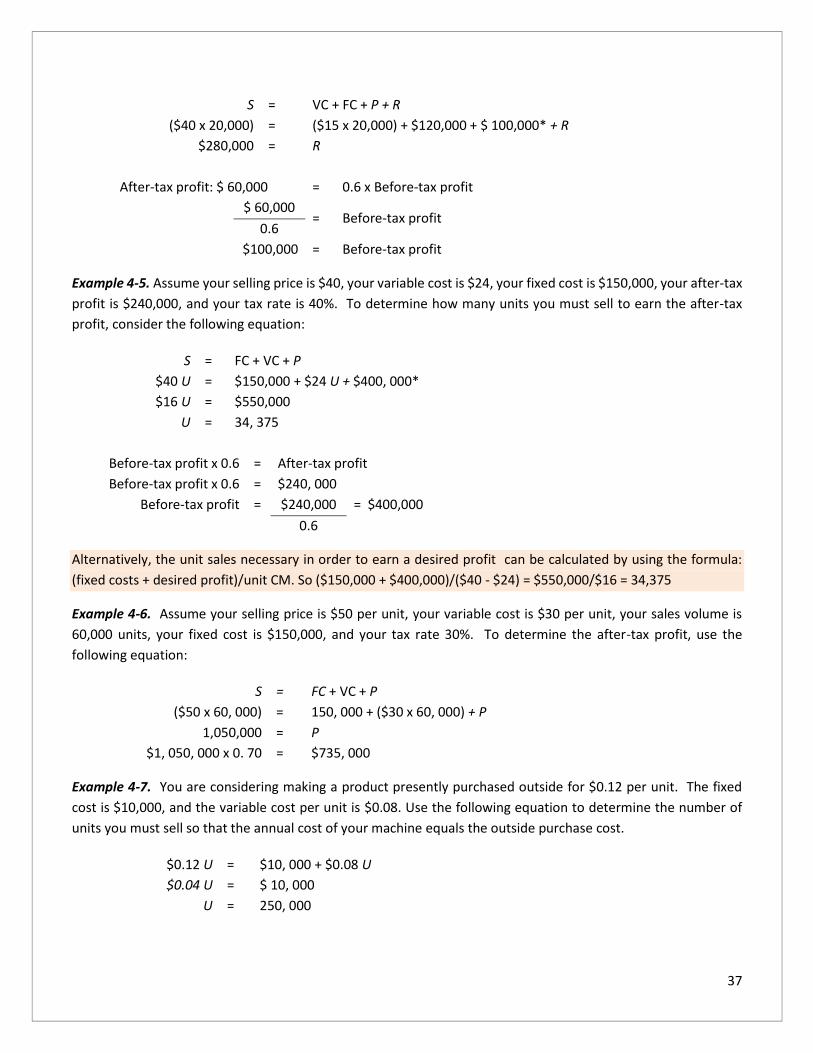
37

S = VC + FC + P + R

($40 x 20,000) = ($15 x 20,000) + $120,000 + $ 100,000* + R

$280,000 = R

After-tax profit: $ 60,000 = 0.6 x Before-tax profit

$ 60,000 = Before-tax profit

0.6

$100,000 = Before-tax profit

Example 4-5. Assume your selling price is $40, your variable cost is $24, your fixed cost is $150,000, your after-tax

profit is $240,000, and your tax rate is 40%. To determine how many units you must sell to earn the after-tax

profit, consider the following equation:

S = FC + VC + P

$40 U = $150,000 + $24 U + $400, 000*

$16 U = $550,000

U = 34, 375

Before-tax profit x 0.6 = After-tax profit

Before-tax profit x 0.6 = $240, 000

Before-tax profit = $240,000 = $400,000

0.6

Alternatively, the unit sales necessary in order to earn a desired profit can be calculated by using the formula:

(fixed costs + desired profit)/unit CM. So ($150,000 + $400,000)/($40 - $24) = $550,000/$16 = 34,375

Example 4-6. Assume your selling price is $50 per unit, your variable cost is $30 per unit, your sales volume is

60,000 units, your fixed cost is $150,000, and your tax rate 30%. To determine the after-tax profit, use the

following equation:

S = FC + VC + P

($50 x 60, 000) = 150, 000 + ($30 x 60, 000) + P

1,050,000 = P

$1, 050, 000 x 0. 70 = $735, 000

Example 4-7. You are considering making a product presently purchased outside for $0.12 per unit. The fixed

cost is $10,000, and the variable cost per unit is $0.08. Use the following equation to determine the number of

units you must sell so that the annual cost of your machine equals the outside purchase cost.

$0.12 U = $10, 000 + $0.08 U

$0.04 U = $ 10, 000

U = 250, 000

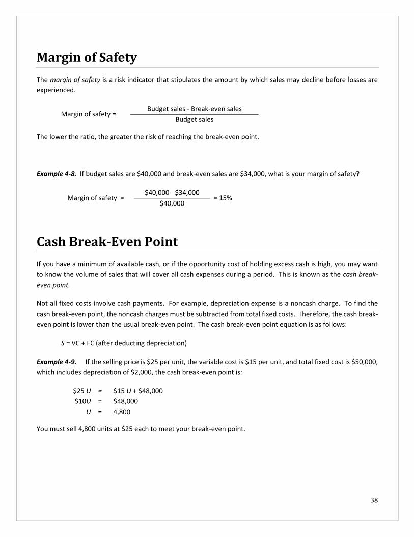
38

Margin of Safety

The margin of safety is a risk indicator that stipulates the amount by which sales may decline before losses are

experienced.

Margin of safety = Budget sales - Break-even sales

Budget sales

The lower the ratio, the greater the risk of reaching the break-even point.

Example 4-8. If budget sales are $40,000 and break-even sales are $34,000, what is your margin of safety?

Margin of safety = $40,000 - $34,000

= 15% $40,000

Cash Break-Even Point

If you have a minimum of available cash, or if the opportunity cost of holding excess cash is high, you may want

to know the volume of sales that will cover all cash expenses during a period. This is known as the cash break-

even point.

Not all fixed costs involve cash payments. For example, depreciation expense is a noncash charge. To find the

cash break-even point, the noncash charges must be subtracted from total fixed costs. Therefore, the cash break-

even point is lower than the usual break-even point. The cash break-even point equation is as follows:

S = VC + FC (after deducting depreciation)

Example 4-9. If the selling price is $25 per unit, the variable cost is $15 per unit, and total fixed cost is $50,000,

which includes depreciation of $2,000, the cash break-even point is:

$25 U = $15 U + $48,000

$10U = $48,000

U = 4,800

You must sell 4,800 units at $25 each to meet your break-even point.

39

Operating Leverage

Operating Leverage measures the percentage change in profits resulting from a percentage change in sales. It is

the degree to which fixed costs exist in your cost structure. It is the extent to which you commit yourself to high

levels of fixed costs other than interest payments in order to leverage profits during good times. However, high

operating leverage means risk because fixed costs cannot be decreased when revenue drops in the short run.

A high ratio of fixed cost to total cost over time may cause variability in profit. But a high ratio of variable cost to

total cost indicates stability. It is easier to adjust variable cost than fixed cost when demand for your products

decline.

Example 4-10. Assume that fixed costs were $40,000 in 20X1 and $55,000 in 20X2, and that variable costs were

$25,000 in 20X1 and $27,000 in 20X2.

The operating leverage in 20X2 compared to 20X1 was higher, as indicated by the increase in the ratio of fixed

costs to total costs. Hence, there is greater earnings instability.

$55,000 = 67.1 % for 20X2

$82,000

$40,000 = 61.5% for 20X1

$65,000

Example 4-11. Assume that your selling price is $30 per unit, your variable cost is $18 per unit, your fixed cost is

$40,000, and your sales volume is 8,000 units. You can determine the extent of operating leverage as follows:

(Selling price - Variable cost) (Units)

(Selling price - Variable Cost) (Units) - Fixed cost

($30 - $18)(8,000) =

$96,000 = 1.71

($30-$18) (8,000) - $40,000 $56,000

This means that for every 1% increase in sales above the 8,000-unit volume, income will increase by 1.71 %. If

sales increase by 10%, net income will rise by 17.10%.

40

Example 4-12. You are evaluating operating leverage. Your selling price is $2 per unit, your fixed cost is

$50,000, and your variable cost is $1.10 per unit, The first example assumes a sales volume of 100,000 units; the

second assumes a sales volume of 130,000 units.

Sales Volume

(in dollars) - Fixed Cost - Variable Cost = Net Income

(100,000 x $2) - $50,000 - $110,000 = $40,000

(130,000 x $2) - $50,000 - $143,000 = $67,000

The ratio of the percentage change in net income to the percentage change in sales volume is as follows:

Change in net income

=

$67,000 - $40,000

=

$27,000

=

Net Income $40,000 $40,000 67.5%

Change in quantity $130,000 - $100,000 $30,000 30.0%

Quantity $100,000 $100,000 = 2.25

If fixed cost remains the same, the 2.25 figure tells you that for every 1% increase in sales above the 100,000-unit

volume there will be a 2.25% increase in net income. Thus, a 10% jump in sales will boost net income by 22.5%.

The same proportionate operating leverage develops regardless of the size of the sales increase above the

100,000-unit level.

The opportunity to magnify the increase in earnings that arises from any increase in sales suggests that you should

use a high degree of operating leverage. Presumably, fixed operating costs should constitute a larger proportion

of the total cost at a particular sales level so as to enhance the gains realized from any subsequent rise in sales.

While a high degree of operating leverage is sometimes a desirable objective, there is the risk of financial damage

caused by a drop in sales. It should also be noted that the more unpredictable sales volume is, the more desirable

it is to have a high degree of operating leverage. Remember: Fixed costs magnify the gain or loss from any

fluctuation in sales.

If you have a high degree of operating leverage, you should not simultaneously use a high degree of financial

leverage (debt) because the combination makes the risk associated with your operations too severe for a volatile

economic environment. Alternatively, if you have a low degree of operating leverage you can often take on a

higher level of financial leverage. The lower risk of operating leverage balances the higher risk of financial leverage

(debt position). The tradeoffs determine how much financial and operating leverage to use.

One example of an operating leverage question you may face is whether to buy buildings and equipment or rent

them. If you buy them, you incur fixed costs even if volume declines. If there is a rental with a short-term lease,

the annual cost is likely to be more, but it is easier to terminate the fixed cost in a business downturn. Another

operating leverage decision involves whether to purchase plant and facilities and manufacture all components of

the product or to subcontract the manufacturing and just do the assembly. With subcontracting, contracts can

be terminated when demand declines. If plant and equipment are bought, the fixed cost remains even if demand

declines.

41

Operating leverage is an issue that directly impacts line managers. The level of operating leverage selected should

not be made without input from the production managers. In general, newer technology has a higher fixed cost

and lower variable cost than older technology. Managers must determine whether the risks associated with

higher fixed costs are worth the potential returns.

Sales Mix Analysis

Break-even analysis requires some additional considerations when your department produces and sells more than

one product. Different selling prices and different variable costs result in different unit contribution margins. As

a result, break-even points vary with the relative proportions of the products sold, called the sales mix. In break-

even analysis, it is necessary to predetermine the sales mix and then compute a weighted average contribution

margin. It is also necessary to assume that the sales mix does not change for a specified period.

Example 4-13. Your department has fixed costs of $76,000 and two products with the following contribution

margin data:

Product A Product B


Less: Variable cost 12 5

Unit contribution margin $ 3 $ 5

Sales mix 60% 40%

The weighted average unit contribution margin is: $3(.6) + $5(.4) = $3.80

Your department's break-even point in units is: $76,000/$3.80 = 20,000 units

which is divided as follows:

Product A: 20,000 units x 60% = 12, 000 units

Product B: 20,000 units x 40% = 8, 000 units

Example 4-14. Your department has total fixed costs of $18,600 and produces and sells three products:

Product A Product B Product C Total

Sales $30,000 $60,000 $10,000 $100,000

Less: Variable cost 24,000 40,000 5,000 69,000

Contribution margin $6,000 $20,000 $ 5,000 $ 31,000

Contribution margin ratio 20% 331/3% 50% 31%

Sales Mix 30% 60% 10% 100%

Since the contribution margin ratio for your department is 31%, the break-even point in dollars is:

42

$18,600/.31 = $60, 000

which will be split in the mix ratio of 3:6:1 to give us the following break-even points for the individual products

A, B, and C:

Product A: $60,000 x 30% = $18,000

Product B: $60,000 x 60% = $36,000

Product C: $60,000 x 10% = $ 6,000

$60,000

One important assumption in a multiproduct department is that the sales mix will not change during the planning

period. If the sales mix does change, however, the break-even point will also change.

Conclusion

If your sales volume consistently exceeds the break-even point, you may improve departmental profitability by

reducing your variable cost of manual labor through a fixed cost investment in plant. However, you must consider

the risk that sales may decline below the break-even point, which will decrease your profitability. Generally, you

should aim to convert fixed cost to variable cost, rather than converting variable cost to fixed. But this must be

done carefully because it will reduce your contribution margin.

43


1. What is the degree or amount that revenues may decline before losses are incurred?

A. Residual income rate

B. Marginal rate of return

C. Margin of safety

D. Target (hurdle) rate of return

2. When does the breakeven point in units increase?

A. When the selling price decreases

B. When the unit variable costs decrease and sales price remains unchanged

C. When the fixed costs remain unchanged and sales price increases

D. When the unit costs increase and sales price increases

3. In calculating the breakeven point for a multiproduct (multiservice) company, which of the following

assumptions is not commonly made when the contribution income statement is used?

A. Selling price is constant

B. Sales volume equals production volume

C. Variable costs are changing per unit

D. A given sales mix is maintained for all volume changes

4. A company increased the selling price of its product from $1.00 to $1.10 a unit when total fixed costs increased

from $400,000 to $480,000 and the variable cost per unit remained unchanged. The breakeven point in units will

be decreased. True or False?

5. What would be the most likely strategy to reduce the breakeven point?

A. Increase both the fixed costs and the contribution margin

B. Decrease both the fixed costs and the contribution margin

C. Decrease the fixed costs and increase the contribution margin

D. Increase the fixed costs and decrease the contribution margin

44

Chapter 5: Cost Data Analysis

Learning Objectives


• Identify relevant costs in the manufacturing process

• Recognize components for making financial decisions

• Identify costs used in future business directions

When analyzing the manufacturing and/or selling functions of your department, you are faced with the problem

of choosing between alternative courses of action. What should you produce? How should you manufacture it?

Where should you sell the product? What price should you charge? In the short run, you may be confronted with

the following non-routine, non-recurring situations:

• Whether to accept or reject a special order

• How to price standard products

• Whether to sell or process further

• Whether to make or buy

• Whether to add or drop a certain product line

• How to utilize scarce resources

This chapter provides guidance to these questions.

The Concept of Relevant Costs

In each of these situations, the ultimate management decision rests on cost data analysis. Cost data, which are

classified by function, behavior patterns, and other criteria, are the basis for profit calculations. However, not all

costs are of equal importance in decision making, and you must identify the costs that are relevant to a decision.

The relevant costs are the future costs that differ between the decision alternatives. Therefore, the sunk costs

are not relevant to these decisions because they are past costs. The incremental or differential costs are relevant

because they are the ones that differ between the alternatives. For example, in a decision on whether to sell an

45

existing business for a new one, the cost to be paid for the new business is relevant. However, the initial cost of

the old business is not relevant because it is a sunk cost.

Under the concept of relevant costs, which may be appropriately titled the incremental, differential, or relevant

cost approach, decision making involves the following steps:

1. Gather all costs associated with each alternative.

2. Drop the sunk costs.

3. Drop those costs that do not differ between alternatives.

4. Select the best alternative based on the remaining cost data.

Example 5-1. You are planning to expand your department’s productive capacity. The plan consists of purchasing

a new machine for $50,000 and disposing of the old without receiving anything. The new machine has a 5-year

life. The old machine has a 5-year remaining life and a book value of $17,500. The new machine will generate the

same amount of revenue as the old one but will substantially cut down on variable operating costs. Annual sales

and operating costs of the present machine and the proposed replacement are based on normal sales volume of

20,000 units and are estimated as follows:

Present Machine New Machine

Sales $60,000 $60,000

Less: Variable costs 35,000 20,000

Less: Fixed costs:

Depreciation (straight-line) 2,500 10,000

Insurance, taxes, etc. 4,000 4,000

Net income $18,500 $26,000

At first glance, it appears the new machine provides an increase in net income of $7,500 per year. However, sales

and fixed costs such as insurance and taxes are irrelevant because they do not differ between the two alternatives.

Eliminating all the irrelevant costs leaves only the incremental costs:

Savings in variable costs $15,000

Less: Increase in fixed costs $10,000*

Net annual cash saving arising from the new machine $5,000

* Exclusive of $2,500 sunk cost

You must also consider that the $50,000 cost of the new machine is relevant; however, the book value of the

present machine is a sunk cost and is irrelevant in this decision.

46

Special Orders vs. Standard Products

Pricing Special Orders

You may receive a short-term, special order for your products at a lower price than usual. Normally, you may

refuse such an order since it will not yield a satisfactory profit. However, if sales are slumping, such an order

should be accepted if the incremental revenue obtained from it exceeds the incremental costs involved. The

company should accept this price since it is better to receive some revenue than to receive nothing at all. A price

that is lower than the regular price is called a contribution price. This contribution approach to pricing is most

appropriate when: (1) there is a distressing operating situation where demand has fallen off, (2) there is idle

capacity, or (3) there is sharp competition or a competitive bidding situation.

Example 5-2. Your department has a 100,000-unit capacity. You are producing and selling only 90,000 units of a

product each year at a regular price of $2. If the variable cost per unit is $1 and the annual fixed cost is $45,000,

the income statement follows:

Total Per Unit

Sales (90,000 units) $180,000 $2.00

Less: Variable costs (90,000 units) 90,000 1.00

Contribution margin $90,000 $1.00

Less: Fixed cost 45,000 0.50

Net income $45,000 $0.50

The company received an order calling for 10,000 units at $1.20 per unit, for a total of $12,000. The buyer will

pay the shipping expenses. Although the acceptance of this order will not affect regular sales, you are reluctant

to accept it because the $1.20 price is below the $1.50 factory unit cost ($1.50 = $1.00 + $0.50). You must consider,

however, that you can add to total profits by accepting this special order even though the price offered is below

the unit factory cost. At a price of $1.20, the order will contribute $0.20 per unit (contribution margin per unit =

$1.20 - $1.00 = $0.20) toward fixed cost, and profit will increase by $2,000 (10,000 units x $0.20). Using the

contribution approach to pricing, the variable cost of $1 will be a better guide than the full unit cost of $1.50. Note

that the fixed costs will not increase.

Per Unit

Without

Special Order

(90k Units)

With

Special Order

(100k Units) Difference

Sales $2.00 $180,000 $192,000 $12,000

Less: Variable costs 1.00 90,000 100,000 10,000

Contribution margin $1.00 $ 90,000 $ 92,000 $ 2,000

Less-. Fixed cost 0.50 45,000 45,000

Net income $0.50 $45,000 $47,000 $2,000

47

Pricing Standard Products

Unlike pricing special orders, pricing standard products requires long-term considerations. The key concept is to

recognize that the established unit selling price must be sufficient in the long run to cover all manufacturing,

selling, and administrative costs, both fixed and variable, as well as to provide for an adequate return and for

future expansion. There are two primary approaches to pricing standard products that are sold on the regular

market, both of which use some kind of cost-plus pricing formula.

1. The full-cost approach defines the cost base as the full unit manufacturing cost. Selling and administrative

costs are provided for through the markup that is added to the cost base.

2. The contribution approach defines the cost base as the unit variable cost. Fixed costs are provided for

through the markup that is added to this base.

Example 5-3. You have prepared the following cost data on your company's regular product:

Per Unit Total

Direct material $6

Direct Labor 4

Variable overhead 4

Fixed overhead (based on 20,000 units) 6 $120,000

Variable selling and administrative expenses 1

Fixed selling and administrative expenses (based on 20,000 units) 2 $40,000

Assume that in order to obtain its desired selling price, the firm has a general policy of adding a markup equal to

50% of the full unit cost or 100% of the unit variable cost.

Under the full-cost approach, the desired unit selling price is:

Direct material $ 6

Direct Labor 4

Factory overhead 10

Full unit cost $20

Markup to cover selling and admin. expenses, and desired profit - 50% of

full unit cost

10

Desired selling price $30

Under the contribution approach, the desired selling price is determined as follows:

Direct material $ 6

Direct Labor 4

Variable costs (overhead, selling, and administrative expenses) __5

Unit variable cost $15

Markup to cover fixed costs, and desired profit- 100% of unit variable cost _15

Desired selling price $30

48

Example 5-4. Your company has determined that a $500,000 investment is necessary to manufacture and market

20,000 units of its product every year. It will cost $20 to manufacture each unit at a 20,000-unit level of activity,

and total selling and administrative expenses are estimated to be $100,000. If your company desires a 20% return

on investment, what will be the markup using the full-cost approach?

Desired rate of return (20% x $500,000)) $100,000

Selling and administrative expenses 100,000

Total $200,000

Full unit cost (20,000 units x $20) $400.000

Required markup (Total/Full unit cost) 50%

Make-or-Buy Decision

Deciding whether to produce a component part internally or to buy it from a supplier is called a make-or-outsource

(buy) decision. This decision involves both qualitative factors (e.g.. product quality and long-term business

relationships with subcontractors) and quantitative factors (e.g., cost). The quantitative effects of the make-or-

buy decision are best seen through incremental analysis.

Examples include:

1. Payroll processing in-house or outsource it to an outside service bureau

2. Developing a training program in-house or sending employees outside for training

3. Providing data processing and network services internally or buying them (Benefits: access to technology

and cost savings)

Other strong candidates for outsourcing include managing fleets of vehicles, sales and marketing, E-commerce,

information technology, human resource, and custodial services. In recent years, companies have been

outsourcing more and more business processes including payroll, employee benefits, customer support, invoicing,

and IT management. Companies claim that outsourcing leads to substantial cost savings, allows them to focus on

their core competencies, and ultimately increases shareholder value.

Example 5-5. You have prepared the following cost estimates for the manufacture of a subassembly component

based on an annual product of 8,000 units:

Per Unit Total

Direct material $ 5 $40,000

Direct labor 4 32,000

variable factory overhead applied 4 32,000

Fixed factory overhead applied

(150% of direct labor cost) 6 $48,000

Total Cost $19 $152,000

49

A supplier offers the subassembly at a price of $16 each. Two-thirds of fixed factory overhead, which represents

executive salaries, rent, depreciation, and taxes, continue regardless of the decision. To determine whether to

make or buy the product, you must evaluate the relevant costs that change between the alternatives. Assuming

productive capacity will be idle if not used to produce the subassembly, the analysis is as follows:

Per Unit Total of 8,000 Units

Make Buy Make Buy

Purchase price 16 128,000

Direct material $ 5 $ 40,000

Direct Labor 4 $ 32,000

Variable overhead 4 $ 32,000

Fixed overhead that can be

avoided by not making 2 $ 16,000

Total relevant costs $15 $16 $120,000 $128,000

Difference in favor of making $ 1 $ 8,000

The make-or-buy decision must be evaluated in the broader perspective of considering how best to utilize

available facilities. The alternatives include:

1. Leaving facilities idle

2. Renting out idle facilities

3. Using idle facilities for other products

Sell or Process Further

When two or more products are produced simultaneously from the same input by a joint process, these products

are called joint products. The term joint costs is used to describe all the manufacturing costs incurred prior to the

point at which the joint products are identified as individual products - that is, the split-off point. At the split-off

point, some of the joint products are in final form and can be sold to the consumer, whereas others require

additional processing.

In many cases, however, you might have an option: you can sell the goods at the split-off point or process them

further in the hope of obtaining additional revenue. Joint costs are considered irrelevant to this sell-or-process-

further decision, since the joint costs have already been incurred at the time of the decision and, therefore,

represent sunk costs. The decision will rely exclusively on additional revenue compared to the additional costs

incurred due to further processing.

Example 5-6. Your company produces products A, B, and C from a joint process. The joint production costs for

the year are $120,000. Product A may be sold at the split-off point or processed further. The additional processing

50

requires no special facilities, and all additional processing costs are variable. The sales value at the split-off point

of 3,000 units is $60,000. The sales value for 3,000 units after further processing is $90,000 and the additional

processing cost is $25,000.

Incremental sales revenue $30,000

Incremental costs of additional processing 25,000

Incremental costs of gain 5,000

It is profitable for product A to be processed further. Keep in mind that the joint production cost of $120,000 is

not included in the analysis, since it is a sunk cost and, therefore, is irrelevant to the decision.

Add or Drop a Product Line

Deciding whether to drop an old product line or add a new one requires an evaluation of both qualitative and

quantitative factors. However, any final decision should be based primarily on the impact on contribution margin

or net income.

Example 5-7. Your department has three major product lines: A, B, and C. You are considering dropping product

line B because it is being sold at a loss. The income statement for these product lines follows:

Product A Product B Product C Total

Sales $10,000 $15,000 $25,000 $50,000

Less: Variable costs 6,000 8,000 12,000 26,000

Contribution margin $ 4,000 $ 7,000 $13,000 $24,000

Less: Fixed costs

Direct $ 2,000 $ 6,500 $ 4,000 $12,500

Allocated 1,000 1,500 2,500 5,000

Total $ 3,000 $ 8,000 $ 6,500 $17,500

Net Income $ 1,000 $(1,000) $ 6,500 $ 6,500

Direct fixed cost are identified directly with each of the product lines, whereas allocated fixed costs are common

fixed costs allocated to the product lines using some base (e.g., space occupied). Common fixed costs typically

continue regardless of the decision and thus cannot be saved by dropping the product line to which they are

distributed.

The following calculations show the effects on your department with and without product line B.

51

Keep Product B Drop Product B Difference Sales $50,000 $35,000 $(15,000) Less: Variable cost 26,000 18,000 (8,000) Contribution margin 24,000 17,000 (7,000) Less: Fixed costs Direct $12,500 $ 6,000 $ (6,500) Allocated 5,000 5,000 Total $17,500 $11,000 $ (6,500) Net Income $ 6,500 $ 6,000 $ 500

Alternatively, if product line B were dropped, the incremental approach would show the following:

Sales revenue lost $15,000

Gains:

Variable cost avoided $8,000

Directed fixed costs avoided 6,500

14,500

Increase (decrease) in net income $ (500)

Both methods demonstrate that by dropping product line B your department will lose an additional $500.

Therefore, product line B should be kept. One of the great dangers in allocating common fixed costs is that such

allocations can make a product line look less profitable than it really is. Because of such an allocation, product

line B showed a loss of $1,000 but it actually contributes $500 ($7,000 - $6,500) to the recovery of common fixed

costs.

Constraining Factors

In general, the emphasis on products with higher contribution margins maximizes your department’s net income.

This is not true, however, when there are constraining factors or scarce resources. A constraining factor is a factor

that restricts or limits the production or sale of a given product. It may be machine hours, labor hours, or cubic

feet of warehouse space. In the presence of these constraining factors, maximizing profit depends on getting the

highest contribution margin per unit of the factor (rather than the highest contribution margin per unit of product

output).

Example 5-8. Your department produces products A and B with the following contribution margins per unit

and an annual fixed cost of $42,000.

Product A Product B

Sales $8 $24

Less: Variable costs 6 20

Contribution margin $2 $ 4

52

As is indicated by the contribution margin, product B is more profitable than product A since it contributes more

to your department's profits ($4 versus $2). But assume that your department has a limited capacity of 10,000

labor hours. Further, assume that product A requires 2 labor hours to produce and product B requires 5 labor

hours. One way to express this limited capacity is to determine the contribution margin per labor hour.

Product A Product B

Contribution margin per unit $2.00 $4.00

Labor hours required per unit 2 5

Contribution margin per labor hour $1.00 $0.80

Since product A returns the higher contribution margin per labor, it should be produced and product B should be

dropped. Another way to look at the problem is to calculate the total contribution margin for each product.

Product A Product B

Maximum possible production 5,000 units* 2,000 units**

Contribution margin per unit x $2 x $4

Total contribution margin $10,000 $8,000

*(10,000 hours/2 hours)

**(10,000 hours/5 hours)

Again, product A should be produced since it contributes more than product B ($10,000 versus $8,000)

In addition to the quantitative factors, qualitative factors must also be considered in decision-making. Qualitative

factors, which are difficult to measure in terms of money, include:

1. Effect on employee morale and schedules

2. Relationships with and commitments to suppliers

3. Effect on present and future customers

4. Long-term future effect on profitability

In some decision-making situations, qualitative factors are more important than immediate financial benefits.

Conclusion

Not all costs are of equal importance in decision making. The relevant costs are the expected future costs that

differ between the decision alternatives. Therefore, the sunk costs are irrelevant since they are past costs. The

costs that continue regardless of the decision are also irrelevant. The relevant cost approach assists you in making

short-term, non-routine decisions such as whether to accept a below-normal selling price, which products to

emphasize, whether to make or buy, whether to sell or process further, and how to optimize utilization of capacity.

In addition to these quantitative aspects, remember qualitative factors must also be considered in many decision-

making situations.

53


1. What are ‘relevant costs’?

A. All fixed and variable costs

B. Expected future costs that will differ among various alternatives

C. Costs that would be incurred within the relevant range of production

D. Past or historical costs that are expected to be different in the future

2. There is a market for both product X and product Y. Which of the following costs and revenues would be most

relevant in deciding whether to sell product X or process it further to make product Y?

A. Total cost of making X and the revenue from the sale of X and Y

B. Total cost of making Y and the revenue from the sale of Y

C. Additional cost of making Y, given the cost of making X, and additional revenue from Y

D. Additional cost of making X, given the cost of making Y, and additional revenue from Y

54

Chapter 6: Financial Forecasting and Budget Planning

Learning Objectives


• Identify the importance and value of sales forecasts

• Recognize how sales forecasts and budgets affect other operational budgets

To accomplish your department’s goals you must be familiar with financial forecasting and budget planning.

Without these instruments, you have no plan on which to base future financial decisions, and without a plan, you

cannot make things happen. As a non-financial manager, you may have to forecast sales, production, and costs

under varying assumptions. This chapter explains how to prepare and use financial forecasts and budgets that

help you accurately plan and control your department’s future.

Benefits of Forecasting

Despite the uncertainties in life, it is important to attempt to forecast what will happen. In fact, forecasting tries

to minimize uncertainty about the future. A forecast is a starting point for planning. It may simply be a projection

that what happened last year will happen this year, or it may be quite complex using statistical techniques and

seasonal patterns. Although you can base your projection on historical patterns, you must also take into account

any important changes taking place in the current environment, as these changes will make the future different

from the past. Examples of relevant changes are better technology, changes in laws and regulations, and

increased competition.

Forecasts are the basis for capacity planning, inventory planning, planning for sales and market share, and

budgeting. Sales forecasts are particularly important in many financial activities including budgets, profit planning,

capital expenditure analysis (whether to buy long-term assets), and acquisition and merger analysis (when two

companies combine into one).

You must realize that forecasts are guesses regarding the future. The guesses principally arise from hard data

rather than from subjective judgment, therefore, certain variables may not be accounted for in this process.

55

Hence, you should question forecasted figures that seem unreasonable and illogical based on your experience.

After all, you are most familiar with the financial factors that relate to your job.

Forecasts are needed for marketing, production, manpower, and financial planning and are used for planning and

implementing long-term objectives. For example:

• If you are a marketing manager, for instance, you can use sales forecasts to determine optimal sales force

allocations, establish sales goals and plan promotions and advertising.

• If you are a production planner, you need forecasts to schedule production activities, order materials, and

plan shipments.

• If you are a purchaser, you need forecasts to aid you in determining what quantity of merchandise is

needed and when to satisfy projected sales.

Figure 6-1 illustrates the relationship between forecasting and managerial functions. For example, as soon as your

company is sure that it has sufficient capacity, the production plan is developed. If the company does not have

enough capacity, planning and budgeting decisions will be required for capital spending to expand capacity.

In planning for capital investments, predictions of economic activity are required so that the returns, or cash

inflows, accruing from the investment may be estimated. Borrowing needs for future operations should also be

estimated through forecasts. Financial managers must make forecasts of money and credit conditions and

interest rates so that the cash needs of the firm may be met at the lowest possible cost (e.g.. should the company

issue stock or debt to maintain its desired financial structure?). Long-term forecasts are needed to plan changes

in the company's capital structure.

Figure 6-1. Sales Forecasts and Managerial Functions

56

Figure 6-2. Sales Forecasts by Product Line

The Financial Forecasting Process

To prepare a financial forecast you must begin by forecasting sales. Production and related cost forecasting will

follow. Forecasting is easiest when there exists stability in relationships that can be captured in mathematical

terms (e.g., sales = a + b (advertising expenses) + c (price)).

The sequence for forecasting financing needs is:

1. Project your sales.

2. Project variables such as cost of sales and operating expenses.

3. Estimate the level of investment in assets required to support the projected sales.

4. Calculate financing needs.

5. Consider external factors affecting the forecast. Political concerns, economic environment, tax law,

technological developments, and demographic factors may be applicable in certain cases.

Most other forecasts (budgets) follow the sales forecast. Sales estimates may be based on several factors

including your instincts, past experiences, feedback from the sales force, and consumer surveys. If any changes

are expected in your product mix (lines added or deleted), the projected change in volume is a consideration in

projecting sales. If competition or cost reductions necessitate price changes, these must also be considered in

making your sales forecast. A sales forecast of major product lines for a 6-month period is shown in Figure 6-2.

57

When constructing a financial forecast, the sales forecast is used to estimate various expenses, assets, and

liabilities. Often, sales forecasting is done by product line. The most widely practiced method for formulating

projections is the percent-of-sales method, in which the various expenses, assets, and liabilities for a future period

are estimated as a percentage of sales for the present period. These percentages, together with the projected

sales for the upcoming year, are then used to construct pro forma (planned or projected) balance sheets.

The computations for a pro forma balance sheet follow:

1. Express balance sheet items that vary directly with sales as a percentage of sales. Any item that does not

vary directly with sales (e.g.. long-term debt) is considered not applicable (NA).

2. Multiply the percentages determined in step I by the projected sales figure to obtain the amounts for the

future period.

3. Where no percentage applies (e.g., for long-term debt, common stock, and paid-in-capital), simply insert

the figures from the present balance sheet in the column for the future period.

4. Compute the projected retained earnings as follows:

Projected retained earnings = present retained earnings

+ projected net income - cash dividends

(You need to know the percentage of sales that represents net income and the dividend payout ratio.)

5. Sum the asset accounts to obtain a total projected assets figure. Then add the projected liabilities and

equity accounts to determine the total financing provided. Since liabilities plus equity must balance the

assets when totaled, any difference is a shortfall, which is the amount of external financing required.

Let us numerically work one out.

Example 6-1. For the pro forma balance sheet shown in Table 6-1 net income is assumed to be 5% of sales and

the dividend payout ratio is 40%.

One important limitation of the percent-of-sales method is that your company is assumed to be operating at full

capacity. Based on this assumption, the firm does not have an adequate production capacity to absorb projected

increases in sales and may require an additional investment in assets.

The prime advantage of the percent-of-sales method of financial forecasting is that it is simple and inexpensive.

To obtain a more precise projection of future financing needs, however, the preparation of a cash budget is

required.

58

Table 6-1. Pro Forma Balance Sheet in Millions of Dollars

Present

(20X8)

% of Sales

(20X8 Sales=$20)

Projected

(20X9 Sales=$24)

Assets

Current assets 2 10 2.4

Fixed assets 4 20 4.8

Total assets 6 7.2

Liabilities and

Stockholders'

Equity

Current liabilities 2 10 2.4

Long-term debt 2.5 N.A. 2.5

Total liabilities 4.5 4.9

Common stock 0.1 N.A. 0.1

Paid-in-capital 0.2 N.A. 0.2

Retained earnings 1.2 1.92 *

Total equity 1.5 2.22

Total liabilities and

stockholders' equity 6 7.12 Total financing provided

0.08 **External financing

needed

7.2 Total

*20X9 retained earnings = 20X8 retained earnings + projected net income – cash dividends paid

= $1.2 + 5%($24) - 40%[5%($24)]

= $1.2 + $1.2 - $0.48 = $2.4 - $0.48 = $1.92

**External financing needed projected total assets - (projected total liabilities + projected equity)

= $7.2 - ($4.9 + $2.22) = $7.2 - $7.12 = $0.08

59

The Budgetary Process

The Significance of Budgeting

Budgets are very important to non-financial managers. They are useful for planning your goals, evaluating your

progress, motivating your people, and communicating your results. Often your attainment of budget goals is

measured in terms of variances. Budgeting is also very useful on a personal level, as you always want to know

where you are in relation to your goals.

In a personal interview with the author, another non-financial manager commented:

“We use our projected sales forecasts for determining our increase in [insurance] policies in force. I am directly

involved in our direct labor budget as we plan out our total personnel needs. I also must budget what each of my

people will cost the company in terms of salary expense. I must budget for a certain percentage of promotions

and also budget for the dollar amount and frequency of merit increases. This along with other aspects combine to

formulate our yearly plan. After that is established we have everything in terms of variances to plan. Our

management staff is then evaluated on our results in terms of variances. I am responsible for overtime dollars,

additions to staff, and our in-house efficiencies in terms of production plans.”

The budget coordinates the activities of all the departments in your company. It communicates companywide

goals to non-financial managers in different departments so they know what direction to take. You have no choice

but to be familiar with your departmental budget and determine a way to keep within it. Many non-financial

managers also believe that they must use all the money allocated to them in the budget, so as not to lose funding

next year; however, this does not mean that funds should be spent foolishly just to meet the budget.

Almost all non-financial managers are responsible for either planning and submitting a budget for a specific period

of time or for conforming to one that has already been laid out.

In a personal interview, a non-financial manager employed by a computer company commented:

“Although the company's attitude toward the budgeting process is a bottom-up approach, the calculation of the

budget is almost entirely a top-down method. My immediate superior hands me the annual budget and discusses

it with me for any discrepancies. Our basic strategy for budgeting can be viewed as follows: first, strategic aspects

are analyzed for both the short and long term; next, specific plans are developed; and last, the actual budgets are

formulated.”

The budget is a blueprint for planning and control. It enables you to see your role and set goals accordingly. At

the beginning of the period, the budget is a standard. If you have no initial plan, you have no idea of what you

want to accomplish. At the end of the period, the budget is a control device to measure your department's

performance against the plan so that future performance may be improved. If you do not know where you are

going, it is hard to tell whether or not you have arrived.

60

The Concept of Budgeting

A budget is an annual projection of what you expect to achieve financially and operationally. It is a plan that

commits resources to activities or projects and makes formal (written) statements of your expectations of sales,

expenses, production, volume, and various financial transactions for the coming period A budget places guidelines

and limitations on spending.

Prior to the budget being developed, certain questions must be asked and certain assumptions must be made:

• What will the inflation rate be?

• Where is competition headed?

• Will suppliers increase prices?

• Will customer tastes change?

You also must explore the financial alternatives available to you. For instance, what will occur if you raise your

selling price? What will be the effect if one variable (e.g., advertising) is changed?

The most common budget types that a non-financial manager might have to deal with are fixed budgets and

flexible budgets. A fixed budget allocates a specific amount of resources that can be used to complete a specific

task - this amount cannot be exceeded. A flexible budget allows the amount of allocated resources to vary along

with the various levels of activity on a specific project.

In a personal interview with the author, a non-financial manager discussed the budgeting process as follows:

“Budgeting at the firm follows the traditional top-down planning strategy. Sales budgets are set up for the firm

as a whole, then broken out into the four sales regions - eastern, central, western, and southern states. In the

Eastern Region, we then receive our share of the corporate budget, which we must then subdivide among the

territories in the region. The two key budgets that must be given considerable thought in their divisions are the

sales quotas themselves and the promotional local funding dollars. Travel and expense dollars for the field

representatives must be allocated. On a less formal, periodic basis, we receive allocations of promotional items

that are charged to a national budget or charged in whole to our region and also must be allocated to the territories

in the region.” A budget should be realistic (e.g., feasible in marketing and production capabilities) and consistent

with company policy. It should take into consideration what your department’s or company's mission is. For

instance, does your company want to hold the line against the competition or does it want to grow? Should your

company take an aggressive or a conservative approach in achieving these goals?

61

The Budgetary Process

The budgetary time period depends on many factors including how crucial the budget is to control costs. The

period for a budget can be any appropriate time frame such as yearly, quarterly, monthly, weekly, and daily.

The major steps in preparing the budget are:

1. Completing a sales forecast

2. Determining expected production volume

3. Estimating manufacturing costs and operating expense

4. Determining cash flow and other financial effects

5. Preparing projected financial statements.

The budgetary process involves establishing goals, developing strategies, noting changes in the customer base,

formulating plans of action, evaluating the market, looking at economic and political conditions, reviewing

suppliers, analyzing competition, appraising industry trends, identifying the life cycle of the product, reviewing

technological changes, appraising financial strength, and taking corrective action. However, without competent

management, budgeting is a waste of time and money. A manager with a poor understanding of budgets may fail

to correctly anticipate the future and commit to objectives for which his or her budget is inadequate, which may

result in a budget overrun.

The budget should be constantly evaluated since external or internal conditions may warrant changes. A budget

is only an estimate, and deviation from that estimate should be expected. The budget must be adaptable to

changing circumstances in your department. What will happen to sales if conditions change? What problems will

be caused if initial sales expectations prove wrong? It is best to develop cost figures for different sales levels (e.g.,

high, low, expected) to assure flexibility.

Components of the Master Budget

The master (comprehensive) budget contains a projection of each of the key financial statements. Supporting

schedules are also prepared for each of the major components in the financial statements. The master budget is

classified broadly into two categories-the operational budget and the financial budget. The operational budget

reflects the results of operating decisions and provides data needed to prepare a budgeted income statement.

The financial budget shows the financial decisions of your company and includes the cash budget and financial

statement projections other than the income statement.

The operational budget includes the following:

1. The sales budget

2. The direct materials budget

3. The direct labor budget

4. The factory overhead budget

5. The selling and administrative expense budget

62

6. The pro forma income statement

The financial budget includes the following:

• The cash budget

• The pro forma balance sheet

A simplified diagram of the various components of the comprehensive budget is shown in Figure 6-3.

Figure 6-3. A Master (Comprehensive) Budget

63

The Operational Budget

Sales Budget

The sales budget is the starting point in preparing the master budget since estimated sales volume influences

nearly all other items appearing in the master budget. The sales budget, which ordinarily indicates the quantity

of each product expected to be sold, allows all departments to plan their needs. A sales forecast is the starting

point for effective inventory management since expected sales determine how much inventory is needed. Further,

sales forecast figures determine staffing needs to reach targeted goals.

Accurate sales forecasting is important since an exaggerated sales forecast may result in your company hiring too

many staff members or acquiring excessive facilities, which translates into unneeded costs. On the other hand, a

very pessimistic forecast may cause a shortage in staff and facilities so that consumer demand cannot be met; this

translates into lost business. Non-financial managers must also carefully appraise the sales estimates of other

departments. For instance, the marketing department may give rosy sales estimates because it may try to

stimulate the sales effort. As a result, it may not realistically appraise consumer demand.

After the sales volume has been estimated, the sales budget is constructed by multiplying the expected sales in

units by the expected unit sales price. Generally, the sales budget includes a computation of expected cash

collections from credit sales, which will be used later for cash budgeting. To illustrate how all these budgets are

put together, we will focus on a manufacturing company called the Johnson Company, which produces and

markets a single product. We will assume that the company develops the master budget in contribution format

for 20X2 on a quarterly basis. We will highlight the variable cost-fixed cost breakdown throughout this example.

Example 6-2. The Johnson Company's sales budget for the year ending December 31, 20X2 is as follows:

Quarter

1 2 3 4 Total

Expected sales in units 800 700 900 800 3,200

Units sales price x $80 x $80 x $80 x $80 x $80

Total sales $64,000 $56,000 $72,000 $64,000 $256,000

The schedule of expected cash collections for the Johnson Company is as follows :

Quarter

1 2 3 4 Total

Accounts receivable (12/31/20X1) $ 9,500a $ 9,500

First quarter sales ($64,000) 44,800b $17,920c 62,720

Second-quarter sales ($56,000) 39,200b $15,680c 54,880

Third-quarter sales ($72,000) 50,400b $20,160c 70,560

Fourth-quarter sales ($64,000) 44,800b 44,800

_______ _______ _______ _______ _______

Total cash collections $54,300 $57,120 $66,080 $64,960 $242,460

64

a All of the $9,500 accounts receivable balance is assumed to be collected in the first quarter. b Of the total quarter's sales, 70% are collected in the quarter of sale. c Of the total quarter’s sales, 28% are collected in the quarter following: the remaining 2% are uncollectible.

Production Budget

After sales are budgeted, the production budget can be determined. The number of units expected to be

manufactured is:

Budgeted sales + desired ending inventory - beginning inventory

Good managers constantly evaluate whether production is on schedule with proposed budgets and make

adjustments accordingly. For example, if a computer on an assembly line is down for an extended period of time,

the manager knows that production and output will probably be low for that time period.

Example 6-3. The Johnson Company's production budget for the year ending December 31, 20X2 is as follows:

Quarter

1 2 3 4 Total

Planned sales (see Example 6-2) 800 700 900 800 3,200

Desired ending inventorya 70 90 80 100b 100c

Total needs 870 790 980 900 3,300

Less: Beginning inventoryd 80 70 90 80 80

Units to be produced 790 720 890 820 3,220

a This figure is calculated as 10% of the next quarter's sales b Estimated. c The ending inventory for the year is the same as the one for the fourth quarter. d The same as the previous quarter's ending inventory.

Direct Material Budget

When the level of production has been computed, a direct material budget should be constructed to show how

much material will be required for production and how much material must be purchased to meet this production

requirement. The purchase will depend on both the expected usage of material and inventory levels. The formula

for the computation of the purchase is a follows:

Purchase in units = Usage + Desired ending material inventory units

- Beginning inventory units

The direct material budget is usually accomplished by a computation of expected cash payments for materials.

65

Example 6-4. The Johnson Company's direct material budget for the year ending December 31, 20X2 is as follows:

a 10 percent of the next quarter’s units needed for production multiplied by 3 (material needs per unit). b Estimated. c The same as the prior quarter’s ending inventory.

The schedule of expected cash disbursements for the Johnson Company is as follows:

Quarter

1 2 3 4 Total

Accounts payable (12/31/20X1) $2,200 $2,200

First quarter purchases ($4,698) 2,349a $2,349b 4,698

Second-quarter purchases ($4,422) 2,211a $2,211b 4,422

Third-quarter purchases ($5,298) 2,649a $2,649b 5,298

Fourth-quarter purchases ($4,928) 2,464a 2,464

Total disbursements $4,549 $4,560 $4,860 $5,113 $19,082

a Of the total quarter’s purchases, 50% are paid for in the quarter of purchases.

b The remaining 50% of a quarter’s purchases are paid for in the following quarter.

Direct Labor Budget

The production requirements provide the starting point for the direct labor budget. To compute direct labor

requirements, the expected production volume for each period is multiplied by the number of direct labor hours

to produce a single unit. The direct labor hours required to meet production needs are then multiplied by the

direct labor cost per hour to obtain budgeted total direct labor costs.

Quarter

1 2 3 4 Total

Units to be produced (see Example 6-3) 790 720 890 820 3,220

Material needs per unit (in lbs.) x 3 x 3 x 3 x 3 x 3

Material needs for production (in lbs.) 2,370 2,160 2,670 2,460 9,660

Desired ending inventory of materials (in lbs.)a 216 267 246 250b 250

Total material needs (in lbs.) 2,586 2,427 2,916 2,710 9,910

Less: Beginning inventory of materials (in lbs.)c 237 216 627 246 237

Materials to be purchased 2,349 2,211 2,649 2,464 9,673

Unit price x $2 x $2 x $2 x $2 x $2

Purchase cost $4,698 $4,422 $5,298 $4,928 $19,346

66

Example 6-5. The Johnson Company's direct labor budget for the year ending December 31, 20X2 is as follows:

Quarter

1 2 3 4 Total

Units to be produced

(see Example 6-3) 790 720 890 820 3,220

Direct labor hours per unit x 5 x 5 x 5 x 5 x 5

Total hours 3,950 3,600 4,450 4,100 16,100

Direct labor cost per hour x $5 x $5 x $5 x $5 x $5

Total direct labor cost $19,750 $18,000 $22,250 $20,500 $80,500

Factory Overhead Budget

The factory overhead budget provides a schedule of manufacturing costs other than direct materials and direct

labor. These costs include factory rent, factory insurance, factory property taxes, and factory utilities. Using the

contribution approach to budgeting requires the development of a predetermined overhead rate for the variable

portion of the factory overhead. In developing the cash budget, remember that depreciation is not a cash outlay;

therefore, it must be deducted from the total factory overhead in computing cash disbursement for factory

overhead.

Example 6-6. To illustrate the factory overhead budget, we will assume the following:

• Total factory overhead budgeted = $6,000 fixed (per quarter) plus $2 per hour of direct labor.

• Depreciation expenses are $3,250 each quarter.

• All overhead costs involving cash outlays are paid for in the quarter incurred.

The Johnson Company's factory overhead budget for the year ending December 31, 20X2 is as follows:

Quarter

1 2 3 4 Total

Budgeted direct labor hours (see

Example 6-5)

3,950 3,600 4,450 4,100 16,100

Variable overhead rate x $2 x $2 x $2 x $2 x $2

Variable overhead budgeted 7,900 7,200 8,900 8,200 32,200

Fixed overhead budgeted 6,000 6,000 6,000 6,000 24,000

Total budgeted overhead 13,900 13,200 14,900 14,200 56,200

Less: Depreciation 3,250 3,250 3,250 3,250 13,000

Cash disbursement for overhead 10,650 9,950 11,650 10,950 43,200

67

Ending Inventory Budget

The desired ending inventory budget provides information for the construction of budgeted financial statements.

Specifically, it will help compute the cost of goods sold on the budgeted income statement. It will also give the

dollar value of the ending materials and finished goods inventory to appear on the budgeted balance sheet.

Example 6-7. The Johnson Company's ending inventory budget for the year ending December 31, 20X2 is as

follows:

The unit variable cost of $41 is computed as follows:

a Variable overhead is applied on the same basis as direct labor hours

Selling and Administrative Expense Budget

The selling and administrative expense budget lists the operating expenses incurred when selling the products

and managing the business. In order to complete the budgeted income statement in contribution format, the

variable selling and administrative expense per unit must be computed.

Example 6-8. The Johnson Company's selling and administrative expense budget for the year ending December

31, 20X2 is shown below.

Ending Inventory Units Unit Cost Total

Direct materials 250 pounds (see Example 6-4) $ 2 $ 500

Finished goods 100 units (see Example 6-3) $ 41 $ 4,100

Total $4,600

Unit Cost Units Total

Direct materials $2 3 pounds 6

Direct labor 5 5 hours 25

Variable overhead 2 5 hoursa 10

Total variable manufacturing cost $41

68

Quarter

1 2 3 4 Total

Expected sales in units 800 700 900 800 3,200

Variable selling and

administrative expense per unitsa x $4 x $4 x $4 x $4 x $4

Budgeted variable expense $3,200 $2,800 $3,600 $3,200 $12,800

Fixed selling and admin. expenses

Advertising 1,100 1,100 1,100 1,100 4,400

Insurance 2,800 2,800

Office salaries 8,500 8,500 8,500 8,500 34,000

Rent 350 350 350 350 1,400

Taxes 1,200 1,200

Total budgeted selling and

administrative expensesb $15,950 $12,750 $14,750 $13,150 $56,600

a Includes sales agents' commissions, shipping, and supplies.

b Paid for in the quarter incurred.

Budgeted Income Statement

The budgeted income statement summarizes the various component projections of revenue and expenses for the

budgeting period (for control purposes the budget can be divided into quarters or even months depending on

need).

Example 6-9. The Johnson Company's budgeted income statement for the year ending December 31, 20X2 is as

follows:

Example No.

Sales (3,200 units @ $80) 6-2 $256,000

Less: Variable expenses

Variable cost of goods sold

(3,200 units @ $41) 6-7 $131,200

Variable selling & administrative 6-8 12,800 144,000

Contribution margin 112,000

Less: Fixed expenses

Factory overhead 6-6 24,000

Selling and Administrative 6-8 43,800 67,800

Net operating income 44,200

Less: Interest expense 6-10 425

Net income before taxes 43,775

Less: Income taxes 20% 8,755

Net income 35,020

69

The Financial Budget

Cash Budget

The cash budget is prepared to forecast financial needs. It is a tool for cash planning and control and for

formulating investment strategies. Because the cash budget details the expected cash receipts and disbursements

for a designated time period, it helps avoid the problem of either having idle cash on hand or suffering a cash

shortage.

If a cash shortage is experienced, the cash budget indicates whether the shortage is temporary or permanent and

whether short-term or long-term borrowing is needed. Is a line of credit necessary? Should capital expenditures

be cut back? If the cash position is very poor, the company may even go out of business because it cannot pay its

bills. On the other hand, if the cash position is excessive, the company may be missing opportunities to use its

cash for the greatest profit possibilities. Just as forecasts must be continuously evaluated for changing internal

and external circumstances, the cash budget must also be periodically updated for changing conditions.

A cash budget for your department is similar to a cash budget you would prepare for yourself. To the beginning

cash balance, you add the period's cash receipts, which gives you the total amount available to spend. You then

subtract cash payments, leaving the ending cash balance. Just as you pay cash for living costs (e.g., food and

shelter), a company also pays cash to operate and generate revenue (e.g., advertising). Unlike your personal cash

budget, however, the company's cash budget cannot count on receiving a paycheck each period; you instead must

estimate when credit sales will be collected. However, a company has more alternative sources of cash than you

do. For example, a company may issue stock but a person doesn't.

The cash budget usually is comprised of four major sections:

1. The receipts section gives the beginning cash balance, cash collections from customers, and other

receipts (e.g., borrowing money, selling assets). Note that cash receipts are not necessarily the same

as revenue (e.g. credit sales).

2. The disbursements section shows all cash payments listed by purpose. Examples include cash

expenses, purchase of assets, and payment of debt. Note that not all expenses are cash payments

(e.g., depreciation).

3. The cash surplus or deficit section simply shows the difference between the cash receipts section and

the cash disbursements section.

4. The financing section provides a detailed account of the borrowings and repayments expected during

the budget period.

Example 6-10. To illustrate the cash budget, we will make the following assumptions:

The company desires to maintain a $5,000 minimum cash balance at the end of each quarter.

70

All borrowing and repayment must be in multiples of $500 at an interest rate of 10% per annum. Interest is

computed and paid as the principal is repaid. Borrowing takes place at the beginning of each quarter, and

repayment is made at the end of each quarter.

The Johnson Company's cash budget for the year ending December 31, 20X2 is shown as follows:

Quarter

Example

No. 1 2 3 4 Total

Cash balance, beginning Given $10,000 $9,401 $5,461 $9,106 $10,000

Receipts:

Collection from customers 6-2 54,300 57,120 66,080 64,960 242,460

Total cash available 64,300 66,521 71,541 74,066 252,460

Less: Disbursements:

Direct materials 6-4 4,549 4,560 4,860 5,113 19,082

Direct labor 6-5 19,750 18,000 22,250 20,500 80,500

Factory overhead 6-6 10,650 9,950 11,650 10,950 43,200

Selling and Administrative 6-8 15,950 12,750 14,750 13,150 56,600

Machinery purchase Given 24,300 24,300

Income Tax Given 4,000 4,000

Total disbursements 54,899 69,560 53,510 49,713 227,682

Cash surplus (deficit) 9,401 (3,039) 18,031 24,353 24,778

Financing:

Borrowing 8,500 8,500

Repayment (8,500) (8,500)

Interest (425) (425)

Total financing 8,500 (8,925) (425)

Cash balance, ending $9,401 $5,461 $9,106 $24,353 $24,353

Budget Balance Sheet

The budgeted balance sheet alerts you to unfavorable financial conditions that you might want to avoid. It also

serves as a final check on the mathematical accuracy of all the other schedules, helps you perform a variety of

ratio calculations, and highlights future resources and obligations. The budgeted balance sheet is prepared by

adjusting the previous year's balance sheet based on expectations for the budgeting period.

Example 6-11. To illustrate, we will use the Johnson Company's balance sheet as of December 31 20X1.

71

Assets Liabilities and Stockholders’ Equity

Current assets: Current liabilities:

Cash $10,000 Accounts payable $2,200

Accounts receivable 9,500 Income tax payable 4,000

Material inventory 474 Total current liabilities 6,200

Finished goods inventory 3,280 Stockholders’ equity:

Total current assets 23,254 Common stock, no-par 70,000

Fixed assets: Retained earnings 37,054

Land 50,000

Buildings and equipment 100,000

Accumulated depreciation (60,000)

Total fixed asset 90,000 _______

Total assets 113,254


stockholders’ equity 113,254

The Johnson Company's budgeted balance sheet as of December 31, 20X2 is shown as follows:

Assets Liabilities and Stockholders’ Equity

Current assets: Current liabilities:

Cash $24,353a Accounts payable $2,464h

Accounts receivable 23,040b Income tax payable 8,755i

Material inventory 500c Total current liabilities 11,219

Finished goods inventory 4,100d Stockholders’ equity:

Total current assets $ 51,993 Common stock, no-par 70,000j

Fixed assets: Retained earnings 72,074k

Land 50,000e

Buildings and equipment 124,300f

Accumulated depreciation (73,000)g

Total fixed assets 101,300

_______ ________

Total assets $153,293


stockholders’ equity $153,293 a From Example 6-10 (cash budget). b $9,500 + $256,000 sales(from Example 6-2) - $242,460 receipts(from Example 6-2) = $23,040. c From Example 6-7 (ending inventory budget). d From Example 6-7 (ending inventory) e No change.

f $100,000 + $24,300 (from Example 6-10) = $124,300. g $60,000 + $13,000 (from Example 6-6) = $73,000: h $2,200 + $19,346 (from example 6-4) - $19,082 (from Example 6-4) = $2,464 (all accounts payable relate

to material purchases), or 50% of fourth quarter purchase = 50% ($4,928) = 2,464. i From Example 6-9 (budgeted income statement).

72

j No change. k $37,054 + $35,020 (from Example 6-9) net income = $72,074.

Other Considerations

There is a shortcut approach that is widely used in formulating a budget. In the first step of this approach, a pro

forma income statement is developed using past percentage relationships between relevant expense and cost

items and sales. These percentages are then applied to forecasted sales. This is a version of the percent-of-sales

method previously discussed. Second, a pro forma balance sheet is estimated by determining the desired level of

certain balance sheet items and by making additional financing conform to those desired figures. Thus, the

remaining items are estimated to make the balance sheet balance. There are two basic assumptions underlying

this approach:

1. Previous financial condition is a reliable predictor of a future condition.

2. The value of certain variables (e.g., cash, inventory, and accounts receivable) can be forced to take on

specified desired values.

For smaller companies, a spreadsheet may be used to efficiently and quickly develop a budget. Such software

helps carry out tedious calculations. More importantly, if a budgetary figure is changed (e.g., sales), the

spreadsheet will change all other budgetary amounts related to it (e.g., cost of sales, selling expenses). Hence, it

is easy to make different sales projections and see what the resulting costs and profitability will be.

The computer-based quantitative model is used to construct a profit planning budget and to help answer a variety

of “what-if” questions. Its calculations provide a basis for choosing among alternatives under conditions of

uncertainty. There are primarily two approaches to modeling the corporate budgeting process: simulation and

optimization (see an advanced finance text for more information on these models). There are many user-oriented

modeling languages and packages on the market specifically designed for budgeting.

Conclusion

Budgets should be participative not authoritative, and the budget process should be decentralized to

departmental cost centers with responsible managers. If the people operating under the budget have helped

prepare it, they will be more receptive to meeting the objectives. Budgets must also be realistic if they are to be

accepted by the staff and if the company's objectives are to be met. If you feel a budget is fair and you have

participated in the budgetary process, you can better understand the impact of your decisions on your

department, on other departments, and on the company. You can also determine how best to use allocated funds

to strengthen your departments' position. A budget helps you direct attention from the present to the future. It

assists you in anticipating problems in time to deal with them effectively, and it reveals whether you can expand.

Further, the budget helps you achieve departmental goals. You have a reference point for control reporting. The

budgetary process also assists you in searching for weaknesses, which you can strengthen before they become a

major problem.

73


1. The master budget ___________

A. Shows forecasted and actual results.

B. Contains the operating budget.

C. Reflects controllable costs only.

D. Can be used to determine manufacturing cost variances.

2. What does the master budget process usually begin with?

A. Sales budget

B. Production budget

C. Overhead budget

D. Cash budget

3. A company had sales last year of $10 million, with net income equal to 6% of sales. This year the sales are

expected to be $11.2 million. The accounts receivable balance was $1.5 million at the end of last year. Using the

percentage-of-sales method, what is the accounts receivable balance at the end of this year forecasted to be?

A. $1.572 million

B. $1.68 million

C. $2.172 million

D. $2.7 million

4. Identify the statement below that represents a required underlying assumption for using the percentage-of-

sales technique to develop pro forma financial statements.

A. Economies of scale exist in the use of assets.

B. Your company is assumed to be operating at full capacity.

C. Technological considerations dictate that fixed assets be added in large, discrete amounts.

D. Actual sales-to-asset ratios for the firm in any given period vary with different stages of the economic

cycle.

74

Chapter 7: Cost Control and Variance Analysis

Learning Objectives


• Identify variance analysis and its usefulness to financial analysis

• Recognize when variance analysis should be applied

• Identify cost variances

Variance analysis is a tool managers use to evaluate financial performance. You can carry out variance analysis for

such areas of the company as sales, purchasing, and distribution. Variance analysis can also help you appraise the

productivity of your employees, including sales personnel, factory workers, and delivery personnel, among others.

By using variance analysis, you can spot and correct problems, as well as identify areas of success.

This chapter covers the following topics:

• The standards of revenue and cost

• The use of variance analysis to monitor performance

• The evaluation of sales and cost variances

• The use of flexible budgeting

• Analysis of warehouse problems and sales performance

You will learn to calculate and appraise variances so as to answer these questions:

1. Do your actual sales and expenses match your estimates? Why or Why not?

2. Is the variance favorable or unfavorable? If it is favorable, who should get credit for it? If it is unfavorable,

is it controllable?

3. Is the variance uncontrollable because of external factors such as a strike?

4. Are your standards too tight?

5. What trends do the variances reveal?

6. If the variance is significant (or controllable), what are the reasons and who is responsible? What

corrective actions should be taken?

75

Benefits of Variance Analysis

Locating deviations between expected and actual figures through variance analysis helps you not only to identify

problems but also to determine how large the problem is, who is responsible, and whether it is controllable or

not. For example, if the cost of manufacturing a product or rendering service is higher than expected, you would

want to know the reasons for the discrepancy and the severity of the situation. With the aid of variance analysis,

you can then decide whether the problem lies with buying or planning or general productivity. Or perhaps you

find that actual sales fall short of expectations. You would want to know whether the sales manager can control

the problem (e.g., poor salesperson effort) or not (e.g., an economic depression).

Variance analysis also spotlights positive performances. If the actual cost of a product is less than expected, for

instance, you would want to know what you and your employees are doing correctly so as to capitalize on the

situation. In this event, you would want to reward superior performances by employees or to know that the

company is using new technological processes that successfully keep costs down.

Setting standards and analyzing variances are essential in financial analysis and decision making. Both activities

tell you how you are doing and what is going wrong or right. Although standard costing and variance analysis are

exceptionally important tools, they can have their drawbacks. For example, biases in deriving standards can exist.

Further, material variances can sometimes be due to out-of-date standards or poor budgetary processes rather

than actual performances. Therefore, you should use these tools with caution.

In summary, advantages of standards and variances include:

• If properly used, standards can help motivate employees.

• Assist in decision making because areas of inefficiency are identified.

• Help formulate sales price because you can determine what the item should cost.

• Set and evaluate objectives by comparing budgeted to actual figures.

• Establish cost control since cost inefficiencies and overruns are pinpointed.

• Highlight problem areas through the "management by exception" principle.

• Pinpoint responsibility for undesirable performance so that corrective action may be taken. Variances in

product activity (cost, quantity, quality) are typically the foreman's responsibility. Variances in sales are

often the responsibility of the marketing manager. Variances in profit usually relate to overall operations.

Note that variances indicating strengths should be further taken advantage of.

• Facilitate communication within the organization, such as between management and supervisors,

because everyone knows the standard to accomplish.

• Assist in planning by forecasting needs (e.g., cash requirements).

• Establish bid prices on contracts because desired profit goals can be determined.

• Simplify bookkeeping procedures by keeping the records at the standard cost.

In an interview, a non-financial manager neatly summarized the virtues of variance analysis, which you are about

to learn:

76

“Let’s say production has dropped and I am below plan. I must take appropriate action to get back on course. We

have a weekly production meeting where we must report on our variances to plan in a number of areas. We do

this in order to maintain tight management control and also to be responsive to our changing environment. Also,

this is a very important tool for planning as each week determines the best use for our resources, budgeting our

people if you will.”

Setting Standards

At the beginning of the period, you set standards such as sales quotas, standard costs (e.g., material price, wage

rate), and standard volume. Let us focus on standard cost, which is the predetermined cost of manufacturing,

servicing, or marketing an item during a given future period. It is based on current and projected conditions. This

norm is also dependent upon quantitative and qualitative measurements (e.g., working conditions). A non-

financial manager commented in an interview that his facilities department uses standard costs for equipment

installation and relocation to determine the cost to charge to the ordering unit. For determining the projected

cost of a job, you should understand the concept of and calculations for standard costs.

There are four types of standards:

Basic. These are not changed from period to period. They form the basis with which later period

performance is compared. No consideration, however, is given to a change in the environment, which is

an unrealistic basis.

Maximum efficiency. These are perfect standards, which assume ideal, optimal conditions. Realistically,

certain inefficiencies will occur.

Currently attainable. These are based on efficient activity. They are possible goals but difficult to achieve.

Normal occurrences, such as anticipated machinery failure, are considered in the calculation of currently

attainable standards.

Expected. These are expected figures, which should come very close to actual figures.

You should base standards on the situation being appraised. Here are some examples of how to match standards

with particular situations:

Situation Standard

Cost reduction Tight

Pricing policy Realistic

High-quality Perfection

77

Analyzing Variances

Typically, only significant variances warrant investigation. Further, variances should be investigated when they

fall out of the accepted range or the control limit. To help you interpret variance analysis reports, understand

which variances are important for your position, and remedy any problems.

There are two types of variances: material and immaterial. For material variances, you must identify the

responsible departments or persons and take corrective action. Insignificant, or immaterial, variances need not

be looked into further unless they recur and/or reflect potential difficulty. One way to measure if a variance is

significant is to divide the variance by the standard cost. Generally, a variance of more than 5 percent may be

deemed material. In some cases, materiality is measured by dollar amount or by volume level. For example, the

company may set a policy looking into any variance that exceeds $10,000 or 20,000 units, whichever is less.

Guidelines for materiality should be set to reflect the importance of an element to the corporation's performance

and decision making. For example, when a product or activity is critical to the proper functioning of the business

(e.g., critical part, promotion, repairs), limits for materiality should be such that early reporting of variances is

encouraged. Further, statistical techniques can be used to ascertain the significance of cost and revenue

variances.

Variance analysis compares standard to actual costs or performances. Contingent on the cost-benefit relationship,

these analyses may be as detailed as necessary. Evaluation of variances may be done yearly, quarterly, monthly,

daily, or hourly, depending on how quickly you need to identify a problem. But since you do not know actual

figures (e.g., hours spent) until the end of the period, variances can only be arrived at then.

Sales Variances

Actual and budgeted sales figures should be compared by territory, salesperson, and product to see if

expectations are being realized.

To evaluate sales performance, you should focus on profitable sales volume. Don't be misled by high sales volume;

high sales volume does not automatically mean high profits because the high costs associated with products need

to be subtracted. Thus, reports by salespersons should show not only revenue derived but also gross profit

earned. Although gross profit may not necessarily translate into net profit because of high selling and advertising

expenses, it is a legitimate measure of performance. Overall, the report will reveal where to put sales effort.

When you appraise changes in gross profit, you have to recognize that these changes may be caused by changes

in sales mix, selling price, volume, or returns. Also, a complete analysis of sales volume should include

consideration of budgets, standards, sales plans, industry comparisons, and manufacturing costs.

Sales variances are computed to gauge the performance of the marketing function.

78

Example 7-1. Western Corporation’s budgeted sales for 20X1 were

Product A: 10,000 units at $6.00 per unit $ 60,000

Product B: 30,000 units at $8.00 per unit 240,000

Expected sales revenue $300,000

Actual sales for the year were

Product A: 8,000 units at $6.20 per unit $ 49,600

Product B: 33,000 units at $7.70 per unit 254,100

Actual sales revenue $303,700

There is a favorable sales variance of $3,700, consisting of the sales price variance.

The sales price variance equals: (Actual selling price - Budgeted selling price) x Actual units sold

Product A ($6.20 - $6.00) x 8,000 $1,600 Favorable

Product B ($7.70 - $8.00) x 33,000 9,900 Unfavorable

Sales price variance $8,300 Unfavorable

The sales volume variance equals: (Actual quantity - Budgeted quantity) x Budgeted selling price

Product A (8,000 - 10,000) x $6.00 $12,000 Unfavorable

Product B (33,000 - 30,000) x $8.00 24,000 Favorable

Sales volume variance $12,000 Favorable

By looking at the trend in sales, you may identify unfavorable trends requiring a reduction of the sales effort or a

change in product.

You have to evaluate the meaning of sales variances to your department. For example, an unfavorable sales

volume variance may arise from poor marketing procedures. An unfavorable total sales variance may signal a

problem with the marketing manager because he or she has control over sales, advertising, and often pricing.

Unfavorable sales situations may also be caused by a lack of quality control, substitution of poorer quality

components because of deficient purchasing, or deficient product design based on poor engineering.

You should also compare your divisional sales figures with the sales figures of competing companies' divisions and

with industry averages. Sometimes an unfavorable sales volume variance is caused by the price cuts of competing

companies. And, if unfavorable volume variance is coupled with favorable price variance, you may have lost sales

by raising your prices.

Cost Variances

When a product is made or a service is performed, you have to determine these three cost measures:

79

1. Actual cost equals actual price times actual quantity, where actual quantity equals actual quantity per unit

of work times actual units of work produced

2. Standard cost equals standard price times standard quantity, where standard quantity equals standard

quantity per unit of work times actual units of work produced.

3. Total cost variance equals actual cost less standard cost.

Total cost variance has two elements: price variance and quantity variance. Price (rate, spending) variance is

calculated as follows:

(Standard price - Actual price) x Actual quantity

Quantity (usage, efficiency) variance is formulated in the following manner:

(Standard quantity - Actual quantity) x Standard price

These figures are computed for both material and labor. Figure 7-1 depicts the variance analysis for total cost.

Figure 7-1. Variance Analysis of Total Cost

80

Materials Variances

The materials price variance allows you to evaluate the activity of the purchasing department and to see the

impact of raw materials cost changes on profitability, while the materials quantity variance helps you to judge the

performance of the production supervisor. Example 7-2 calculates the three types of materials variances you need

to know.

Example 7-2. The standard cost of one unit of output (product or service) was $15, or three pieces at $5 per piece.

During the period, 8,000 units were made. The actual cost was $14 per unit or two pieces at $7 per piece,

Total Materials Variance

Standard quantity x Standard price (24,000 x $5) $120,000

Actual quantity x Actual price (16,000 x $7) 112,000

$ 8,000 F

Materials Price Variance


($5 - $7) x 16,000 $ 32,000 U

Materials Quantity Variance


(24,000 - 16,000) x $5 $ 40,000 F

Unfavorable materials price variances may be caused by one or more of the following factors: inaccurate standard

prices, failure to take a discount on quantity purchases, failure to shop for bargains, inflationary cost increases,

scarcity in raw material supplies resulting in higher prices, and purchasing department inefficiencies.

Unfavorable material quantity variances result from poorly trained workers, improperly adjusted machines, use

of an improper production method, outright waste on the production line, and/or use of a lower grade material,

purchased to save money.

Once the reasons for unfavorable materials variances have been determined, you can then locate the responsible

departments or key personnel:

Reason Responsible Party

Overstated price paid Purchasing

Failure to detect defective goods Receiving

Inefficient labor or poor supervision Foreman

Poor mix in material Production manager

Rush delivery of materials Traffic

Unfavorable quantity variance Foreman

Unexpected change in production volume Sales manager

81

To correct an unfavorable material price variance, you can increase the selling price, substitute cheaper materials,

change a production method or specification, or engage in a cost reduction program. To achieve some of these

ends, you should examine the variability in raw material costs, look at price instability in trade publications, and

emphasize vertical integration to reduce the price and supply risk of raw materials.

Lastly, remember that you cannot control materials price variances when higher prices are caused by inflation or

shortage situations or when rush orders are required by the customer, who will bear the ultimate cost increase.

Labor Variances

The standard labor rate is based on the contracted hourly wage rate. Where salary rates are set by a union

contract, the labor rate variance will usually be minimal. Otherwise, it should be the responsibility of the human

resource department. Labor efficiency standards are typically estimated by engineers based on an analysis of the

production operation.

Labor variances are determined in a manner similar to that of material variances, as illustrated in Example 7-2.

Example 7-3. The standard cost of labor is four hours times $9 per hour, or $36 per unit. During the period, 7,000

units were produced. The actual cost is six hours times $8 per hour, or $48 per unit.

Total Labor Variance

Standard quantity x Standard price (28,000 x $9) $252,000

Actual quantity x Actual price (42,000 x $8) 336,000

$ 84,000 U

Labor Rate Variance


($9 - $8) x 42,000 $ 42,000 F

Labor Efficiency Variance


(28,000 - 42,000) x $9 $126,000 U

Possible causes of unfavorable labor rate variance include the following:

1. an increase in wages,

2. poor scheduling or production resulting in overtime work, and

3. use of workers commanding higher hourly rates than expected.

Possible reasons for labor rate variances can be matched with responsible parties, as follows:


Use of overpaid or an excessive number of Human resource manager or

workers union contract

Poor job descriptions Human resource

82

Overtime Production planning

In the case of a shortage of skilled workers, it may be impossible to avoid an unfavorable labor price variance.

Labor efficiency (quantity) variances can be attributed to one or more of the following:

• Poor supervision

• Use of unskilled workers, who are paid lower rates, or the wrong mixture of labor for a given job

• Use of poor-quality machinery

• Improperly trained workers

• Poor quality of materials requiring more labor time in processing

• Machine breakdowns

• Employee unrest

• Production delays due to power failure

The reasons and responsible parties for unfavorable labor efficiency variances can then be matched in these ways:


Inadequate supervision Foreman

Improper functioning of equipment Maintenance

Insufficient material supply or poor quality Purchasing

Overhead Variances

The overhead variance is comprised of the controllable and volume variances.

Relevant computations follow.

Total overhead variance = Actual overhead vs. Standard overhead (standard hours x standard overhead rate).

Controllable variance = Actual overhead vs. Budget adjusted to standard hours.

Note: Budget adjusted to standard hours equals fixed overhead plus variable overhead (standard hours times

standard variable overhead rate).

Volume variance = Standard overhead vs. Budget adjusted to standard hours.

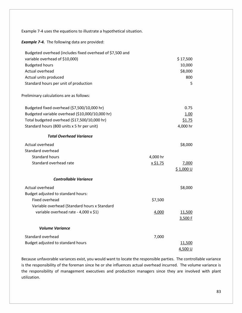
83

Example 7-4 uses the equations to illustrate a hypothetical situation.

Example 7-4. The following data are provided:

Budgeted overhead (includes fixed overhead of $7,500 and

variable overhead of $10,000) $ 17,500

Budgeted hours 10,000

Actual overhead $8,000

Actual units produced 800

Standard hours per unit of production 5

Preliminary calculations are as follows:

Budgeted fixed overhead ($7,500/10,000 hr) 0.75

Budgeted variable overhead ($10,000/10,000 hr) 1.00

Total budgeted overhead ($17,500/10,000 hr) $1.75

Standard hours (800 units x 5 hr per unit) 4,000 hr

Total Overhead Variance


Standard overhead

Standard hours 4,000 hr

Standard overhead rate x $1.75 7,000

$ 1,000 U

Controllable Variance


Budget adjusted to standard hours:

Fixed overhead $7,500

Variable overhead (Standard hours x Standard

variable overhead rate - 4,000 x $1) 4,000 11,500

3,500 F

Volume Variance

Standard overhead 7,000

Budget adjusted to standard hours 11,500

4,500 U

Because unfavorable variances exist, you would want to locate the responsible parties. The controllable variance

is the responsibility of the foreman since he or she influences actual overhead incurred. The volume variance is

the responsibility of management executives and production managers since they are involved with plant

utilization.

84

On the one hand, variable overhead variance information is helpful in arriving at output level and output mix

decisions. It also assists in appraising decisions regarding variable inputs. On the other hand, fixed overhead

variance data provide information regarding decision-making astuteness in relation to the purchase of some

combination of fixed plant size and variable production inputs.

The possible reasons for recurring unfavorable overhead volume variances include the following:

• The purchase of the wrong size plant

• Improper scheduling

• Insufficient orders

• Shortages in material

• Machinery failure

• Long operating time

• Inadequately trained workers

When idle capacity exists, this may indicate long-term operations planning problems.

Static vs. Flexible Budgeting

The static (fixed) budget is geared to only one level of activity and thus has problems in cost control because it

does not distinguish between fixed costs and variable costs.

The flexible budget is geared toward a range of activities rather than a single level of activity. A flexible budget

employs budgeted figures at different capacity levels. It allows you to choose the best expected (normal) capacity

level (100%) and to assign pessimistic (80%), optimistic (110%), and full (150%) capacity levels. You can then see

how your department is performing at varying capacity levels. Fixed costs remain constant as long as you operate

below full capacity.

Flexible budgeting distinguishes between fixed and variable costs, thus allowing for a budget, which can be

automatically adjusted (via changes in variable cost totals) to the particular level of activity actually attained. Thus,

variances between actual costs and budgeted costs are adjusted for volume ups and downs before differences

due to price and quantity factors are computed. Note that flexible budgets are primarily used to accurately

measure performance because they compare actual costs for a given output with the budgeted costs for the same

level of output.

Table 7-1 presents an example of a flexible budget. Example 7-5 illustrates the differences between static and

flexible budgets.

85

Table 7-1. Flexible Budget

Cost

Variable

Cost

Fixed

Cost

Budget

(50,000

hrs.)

Actual

(60,000

hrs.)

Budget

(60,000 hrs.)

Spending

Variance

Indirect material $.80 $6,000 $46,000 $56,000 $54,000 $2,000(U)

Indirect labor 4.20 24,000 234,000 270,000 276,000 6,000(F)

Supervision 70,000 70,000 74,000 70,000 4,000(U)

Depreciation 40,000 40,000 32,000 40,000 8,000(F)

Power and light .30 2,000 17,000 21,000 20,000 1,000(U)

Maintenance 4.70 58,000 293,000 287,000 340,000 53,000(F)

Total $10.00 $200,000 $700,000 $740,000 $820,000 $60,000(F)

Example 7-5. Assume that the Fabricating Department of Company X is budgeted to produce 6,000 units during

June. Assume further that only 5,800 units were produced. The direct labor and variable overhead budget for

the month of June follows:

Budgeted production 6,000 units

Actual production 5,800 units

Direct labor $39,000

Variable overhead costs:

Indirect labor 6,000

Supplies 900

Repairs 300

$46,200

If a static budget is used, the performance report for Company X's Fabricating Department will appear as follows:

Budget Actual Variance (U or F)

Production in units 6,000 5,800 200U

Direct labor $39,000 $38,500 $500F

Variable overhead costs:

Indirect labor 6,000 5,950 50F

Supplies 900 870 30F

Repairs 300 295 5F

$46,200 $45,615 $585F

These cost variances are useless: They compare oranges with apples. That is, the budget costs are based on an

activity level of 6,000 units, whereas the actual costs were incurred at an activity level below this figure (5,800

units). From a control standpoint, it makes no sense to compare costs at one activity level with costs at a different

one. Such comparisons make a production manager look good as long as the actual production is less than the

budgeted production. For our current examples, we should compare costs at the actual production of 5,800 units.

86

Budgeted production =6,000 units

Actual production =5,800 units

Budget Actual Variance

(5,800 units) (5,800 units) (U or F)

Direct labor $6.50 per unit $37,700 $38,500 $800 U

Variable overhead:

Indirect labor 1.00 5,800 5,950 150 U

Supplies .15 870 870 0

Repairs .05 290 295 5 U

$7.70 $44,660 $45,615 $955 U

All cost variances are unfavorable, as compared to the favorable cost variance on the performance report using

the static budget approach.


Marketing Standards and Variances

Prior to setting a marketing standard in a given trade territory, you should examine prior, current, and forecasted

conditions. You should also make adjustments for standards that vary with geographical location. In formulating

standard costs for the transportation function, minimum cost traffic routes should be selected based on the

distribution pattern.

Standards for advertising costs in particular territories will vary depending upon the types of advertising media

needed, which are in turn based on the type of customers the advertising is intended to reach as well as the nature

of the competition.

Some direct selling costs can be standardized, such as product presentations for which a standard time per sales

call can be established. Direct selling expenses should be related to distance traveled, frequency of calls made,

etc. If sales commissions are based on sales generated, standards can be based on a percentage of net sales.

Time and motion studies are usually a better way of establishing sales standards than prior performance, since

past strategies may have been inefficient.

Of the numerous marketing standards and variances, we will focus on, for the purpose of illustration, those

associated with sales.

87

Sales Standards

Sales standards may be set in terms of effort, accomplishments, or the relationship between effort and

accomplishment. For example, a salesperson may be expected to make 100 calls per month. By making 100 calls,

the salesperson meets a standard. He or she may be expected to obtain 60 orders or $300,000 in business based

on the 100 calls. By doing so, a different standard is accomplished. You need to set sales standards to control

sales activities, to reward merit, and to encourage sales effort.

You should appraise sales force effectiveness within a territory, including time spent and expenses incurred.

Examples 7-6 and 7-7 provide you with the data and computations for analyzing variances in two hypothetical

situations.

Example 7-6. Sales data for your department follow.

Standard cost $240,000

Standard salesperson days 2,000

Standard rate per salesperson day $120

Actual cost $238,000

Actual salesperson days 1,700

Actual rate per salesperson day $140

Total Cost Variance

Actual cost $238,000

Standard cost 240,000

$ 2,000 F

Note: Cost variances may be determined by territory, product, or personnel.

The control variance is broken down into salesperson days and salesperson costs.

Variance in Salesperson Days

(Actual days - Standard days) x Standard rate per day

(1,700 - 2,000) x $120 $36,000 F

The variance is favorable because the territory was handled in fewer days than expected.

Variance in Salesperson Costs

(Actual rate - Standard rate) x Actual days

($140 - $120) x 1,700 $34,000 U

An unfavorable variance results because the actual rate per day is greater than the expected rate per day.

Example 7-7. A salesperson called on 55 customers and sold each an average of $2,800 of merchandise. The

standard of calls is 50 and the standard sale is $2,400. Variance analysis of calls and sales follows.

88

Total Variance

Actual calls x Actual sale (55 x $2,800) $154,000

Standard calls x Standard sale (50 x $2,400) 120,000

$ 34,000 F

The $34,000 favorable variance can be broken down as follows.

Variance in Calls

Actual calls - Standard calls) x Standard sale

(55 - 50) x $2,400 $12,000 F

Variance in Sales

(Actual sale - Standard sale) x Standard calls

($2,800 - $2,400) x 50 $20,000 F

Joint Variance

(Actual calls - Standard calls) x (Actual sale - Standard sale)

(55 - 50) x ($2,800 - $2,400) $ 2,000F

You should encourage your sales staff to push products with the highest profitability rather than the highest selling

price or least sales resistance. Additional performance measures of sales force effectiveness include meeting sales

quotas, the number of orders from current and new customers, profitability per order, and the relationship

between salesperson costs and revenue obtained.

Avoid paying your salespeople commissions on gross sales because you may encourage them to sell to anyone,

resulting in huge sales returns and allowances. Instead, the commission should be tied to net sales.

Warehousing Costs Variances

Variance in warehousing costs can be calculated by looking at the cost per unit to store the merchandise and the

number of orders anticipated. Example 7-8 provides the data and calculations of the warehousing cost variance

for a hypothetical situation.

Example 7-8. The following information applies to a product:

Standard cost $12,100

Standard orders 5,500

Standard unit cost $ 2.20

Actual cost $14,030

Actual orders 6,100

Actual unit cost $ 2.30

89

Total Warehousing Cost Variance

Actual cost $14,030

Standard cost 12,100

$ 1,930 U

The total variance is segregated into the variance in orders and variance in cost, as follows.

Variance in Orders

(Actual orders vs. Standard orders) x Standard unit cost

(6,100 vs. 5,500) x $2.20 $1,320 U

Variance in Cost

(Actual cost per unit vs. Standard cost per unit) x

Actual orders ($2.30 vs. $2.20) x 6,100 $ 610 U

Conclusion

Variance analysis is essential for the appraisal of all aspects of the business, including manufacturing, marketing,

and service. Variances are red (or green) flags to watch for and become monitoring and control devices.

Unfavorable variances must be examined to ascertain whether they are controllable by you or uncontrollable

because they solely relate to external factors. When a variance is controllable, immediate corrective action must

be taken to handle the problem. If a variance is favorable, an examination should still be made so that corporate

policy may include the positive aspects. Further, the party responsible for a favorable variance should be

recognized and rewarded.

By looking at variances, you make your department more efficient and less costly to run, with the quality of service

or product at a constant level. You should also determine an acceptable range of variances. Even a small variance

can mean large savings, if favorable, or a large loss, if unfavorable. By analyzing variances, you are using a tool to

protect savings and to cut inefficiencies and losses.

90


1. When preparing a performance report for a cost center using flexible budgeting techniques, what should the

budget cost column be based on?

A. The budgeted amount in the original budget prepared before the beginning of the year.

B. The actual amount for the same period in the preceding year.

C. The budget adjusted to the actual level of activity for the period being reported.

D. The budget adjusted to the planned level of activity for the period being reported.

2. A flexible budget is appropriate for ____________

A. Control of direct materials and direct labor but not selling and administrative expenses.

B. Any level of activity.

C. Control of direct labor and direct materials but not fixed factory overhead.

D. Control of selling and administrative expenses but not factory overhead.

3. Which one of the following is true concerning standard costs?

A. Standard costs are estimates of costs attainable only under the most ideal conditions, but rarely

practicable.

B. Standard costs are difficult to use with a costing system.

C. If properly used, standards can help motivate employees.

D. Unfavorable variances, material in amount, should be investigated, but large favorable variances need not

be investigated.

4. The standard unit cost is used in the calculation of materials price and materials quantity (usage) variances.

True or False?

5. Under a standard cost system, who has responsibility for the materials price variances?

A. Production manager

B. Cost accounting manager

C. Sales manager

D. Purchasing manager

91

6. Under a standard cost system, who has responsibility for the materials usage (quantity) variances?

A. Production supervisor

B. Purchasing and industrial engineering

C. Purchasing and sales

D. Sales and industrial engineering

7. Which of the following could cause an unfavorable direct labor efficiency variance?

A. Unfavorable variable overhead spending variance

B. Favorable variable overhead spending variance

C. Unfavorable fixed overhead volume variance

D. Unfavorable materials quantity (usage) variance

8. How is labor rate variance computed?

A. The difference between standard and actual rates, times standard hours

B. The difference between standard and actual hours, times the actual rate

C. The difference between standard and actual rates, times actual hours

D. The difference between standard and actual hours, times the difference between standard and actual

rates

92

Chapter 8: Financial Assets

Learning Objectives


• Identify components of working capital

• Recognize methods to finance an asset

• Identify ways to improve cash management

• Recognize ways to accelerate cash receipts or delay cash payments

The ability to manage working capital will improve return and minimize the risk of running short of cash. There

are various ways of managing working capital to achieve success. These methods will be discussed in this chapter.

The Concept of Working Capital

A company must maintain a level of working capital sufficient to pay bills as they come due. Failure to do so is

technical insolvency and can result in involuntary bankruptcy. Unfortunately, holding current assets for purposes

of paying bills is not profitable for a company because they usually offer a low return compared with longer-term

investments. Thus, the skillful management of working capital requires a balancing of a firm's desire for profit with

its need for adequate liquidity.

Briefly, working capital equals total current assets - the most liquid assets of the company. Example 8-1 illustrates

how to calculate working capital.

Example 8-1. The following assets exist: $10,000 in cash, $30,000 in accounts receivable, $42,000 in inventory,

$90,000 in machinery, $36,000 in long-term investments, and $4,000 in patents.

The working capital consists of total current assets:

Cash $10,000

Accounts receivable 30,000

Inventory 42,000

93

Total working capital $82,000

When you need funds to buy seasonal inventory, you should finance with short-term debt because the sale of the

inventory will generate funds in the near term to pay off the obligation. The short-term debt provides flexibility

to meet seasonal needs within your ability to repay the loan. Long-term assets should be financed with long-term

debt because the assets last longer and the financing can be spread over a longer time period. These two

strategies are called hedging; that is, you are financing assets with liabilities of similar maturity so the proceeds

and return from the assets may be used to pay off the debt, resulting in less financing risk.

The liquidity of the current assets will influence the terms and availability of short-term credit. The more liquid

your business is, generally the easier it is for you to obtain short-term credit at favorable terms. Short-term credit,

in turn, affects the amount of cash held.

Your working capital needs will partly depend on how long it takes your company to turn raw materials into sold

products. The longer it takes to acquire or produce goods, the greater the working capital needed.

Cash Management

The Nature of Cash Management

Sound cash management requires you to know how much cash is needed, how much cash you have, and where

that cash is. This knowledge is particularly crucial during inflationary periods.

Before you plan a cash management strategy, you need to take care of some basic cash-handling needs. For

example, make certain that cash receipts are deposited promptly. Also, make sure that cash is not unnecessarily

tied up in other accounts such as advances or loans to employees and insurance deposits.

Next, you need to determine your cash management objective. You want to invest excess cash for a return but

have adequate liquidity to meet your needs. Thus, you have to plan when to have excess funds available for

investment and when money needs to be borrowed. But some available cash is needed for unexpected demands

or for customer collection problems.

What determines how much cash you should hold? The key factors are cash management policies, current

liquidity position, liquidity risk preferences, maturity dates of debt, ability to borrow, forecasted short- and long-

term cash flow, and the probabilities of different cash flows under varying circumstances.

You do not want an excessive cash balance because no return can be earned on it. The minimum cash to hold is

the greater of (1) compensating balances (a deposit held by a bank to compensate for providing services) or (2)

precautionary balances (money held for emergency purposes) plus transaction balances (money to cover checks

outstanding).

94

You can get away with a smaller cash balance when cash receipts and cash disbursements are highly synchronized

and predictable. You have to accurately forecast the amount of cash needed, its source, and its destination. These

data are needed on both a short- and a long-term basis. Forecasting assists in properly timing financing, debt

repayment, and the amount to be transferred between accounts.

If you have many bank accounts, you may be able to guard against accumulating excessive balances. You need

less cash on hand if you can borrow quickly from a bank, such as under a line of credit agreement, which allows

you to borrow instantly up to a specified maximum amount. A line of credit is an arrangement between a bank

and a borrower in which the bank commits itself to lend up to a certain maximum amount to the borrower in a

given period.

Warning: Cash in some bank accounts may not be available for investment. For example, when a bank lends you

money, it may require you to retain funds on hand as collateral. This deposit is referred to as a compensating

balance, which in effect represents restricted cash.

Cash management also requires knowing the amount of funds available for investment and the length of time

they can be invested. You can invest funds in the following ways:

• Time deposits, including savings accounts earning daily interest, long-term savings accounts, and

certificates of deposit (short-term, negotiable time deposits with banks, issued at face value and providing

for interest at maturity).

• Money market funds, which are managed portfolios of short-term, high-grade debt instruments such as

Treasury bills and commercial paper.

• Demand deposits that pay interest.

• Bankers' acceptances, which are short-term (up to six months), noninterest-bearing notes up to $1 million

issued at a discount. Acceptances are mostly traded internationally and enjoy their preferred credit status

because of their "acceptance" (guarantee) for future payment by commercial banks. Bankers'

acceptances are time drafts drawn on and accepted by a banking institution, which in effect substitutes

its credit for that of the importer or holder of merchandise.

• Commercial paper, which is a short-term, unsecured debt instrument issued by financially strong

companies (see Chapter 16 for a more detailed discussion).

• Short-term tax exempts issued by states and local government agencies in denominations up to $1 million.

The maturity typically ranges from 6 to 12 months. A good secondary market exists for resale. Interest is

paid at maturity.

• Repurchase agreements issued by dealers in U.S. government securities.

• The maturity ranges from one day to three months. They come in typical amounts of $500,000 or more.

No secondary market exists. They are legal contracts between a borrower (security seller) and the lender

(security buyer). The borrower will repurchase at the contract price plus an interest charge.

• Treasury bills, which are backed by the U.S. government. Treasury bills are issued for terms of 4, 13, 26,

and 52 weeks. They trade in minimum units of $100. Treasury bills are issued at a discount, which means

that interest represents the difference between the price paid and the face value of the instrument at the

95

maturity date. Treasury bills are exempt from state and local income tax. A treasury bill is highly liquid

and nearly risk-free, and it is often held as a substitute for cash.

Example 8-2 demonstrates how to calculate the annual return of a Treasury bill.

Example 8-2. A $10,000, three-month Treasury bill is purchased for $9,800. The return for three months is

Return = $10,000 - $9,800 = $200 = 2%

Investment $9, 800 $9, 800

On an annual basis, the return is: 2% x 12/3 = 8% (annual return)

By holding marketable securities, you can protect against cash shortages. If your business is seasonal, you may

buy marketable securities when excess funds exist and then sell the securities when there is a cash deficit. You

may also invest in marketable securities when funds are being held temporarily in anticipation of short-term

capital expansion. In deciding on an investment portfolio, you should consider the return rate, default risk,

marketability, and maturity date.

In deciding on a cash management system, you should consider its associated costs compared to the return earned

from implementing the system. The costs include bank charges, your time, and office employee salaries. You can

make use of your personal computer in making transactions with the computers of banks and money market

funds. Computer systems are also useful for buying and selling securities in the money market.

The thrust of cash management is to accelerate cash receipts and delay cash payments. Analyze each bank

account as to its type, balance, and cost so that return is maximized.

Accelerating Cash Receipts

To accelerate cash inflow, you must (1) know the bank's policy regarding fund availability, (2) know the source

and location of cash receipts, and (3) devise procedures for the quick deposit of checks received and for quick

transfer of receipts in outlying accounts into the main corporate account.

Note: Electronic data exchange (EDI) or financial EDI (FEDI) significantly reduces or eliminates float. EDI refers to

the practice of direct, electronic information exchange between all types of businesses, thereby shortening the

length of time required to initiate and complete a business transaction. Electronic payments are the fastest way

to reduce float by completing eliminating any physical handling of payments, and the cost savings from reducing

handling expenses, along with faster payments, can greatly outweigh any cost of implementation.

Before you draw up plans for quick deposits and transfers, you need to understand the check processing delays.

Delays include (1) mail float—the time a check moves from a debtor to a creditor, (2) processing float—the time

it takes for a creditor to deposit the check after receipt, and (3) deposit collection (transit) float—the time for a

check to clear.

96

Figure 8-1 illustrates a cash or check collection system for a hypothetical business not using electronic data

exchange.

Figure 8-1. Cash Collection System

You can minimize mail float by making sure that the collection center is close to the customer. Local banks should

be selected to hasten the receipt of funds for subsequent transfer to the central corporate account. Alternatively,

strategic post office lockboxes may be used for customer remissions. The local bank collects from these boxes

periodically during the day and deposits the funds in the corporate account. The bank also provides a computer

listing of payments received by account and a daily total. Because the lockbox system has a significant per-item

cost, it is most effective with low-volume, high-dollar collections. But the system is becoming increasingly more

available to firms with high-volume, low dollar receipts because technological advances (such as machine-

readable documents) are lowering the per-item cost of lockboxes.

Example 8-3 calculates, for a hypothetical situation, the amount of money that can be tied up by mailing delays.

Example 8-3. You obtain average cash receipts of $300,000 per day. It typically takes 6 days from the time a check

is mailed to its availability for use. The amount tied up by the delay is

6 days x $300, 000 = $1,800,000

Before implementing a lockbox system, you need to undertake a cost-benefit analysis considering the average

dollar amount of checks received, the costs saved by having lockboxes, the decline in mailing time per check, and

the processing cost. Figure 8-2 depicts a simple lockbox system.

97

Figure 8-2. Lockbox System

Example 8-4 shows you how to calculate the maximum monthly payment for a lockbox.

Example 8-4. It takes about eight days to receive and deposit payments from customers. Thus, a lockbox system

is being considered. It is anticipated that the system will reduce the float time to five days. The average daily

collections are $400,000. The return rate is 11%.

The reduction in outstanding cash balances occurring if the lockbox system is initiated is

3 days x $400,000 = $1,200,000

The return that could be earned on these funds is

$1,200,000 x .11 = $132, 000

The maximum monthly charge that should be paid for the lockbox arrangement is therefore

$132,000 / 12 = $11,000

Example 8-5 illustrates the financial advantage of a lockbox system.

Example 8-5. You are considering the use of a lockbox system costing $130,000 per year. Daily collections average

$360,000. The lockbox arrangement will reduce the float period by three days. The rate of return is 14%.

The cost-benefit analysis is shown below:

Return on early collection of cash (. 14 x 3 x $360,000) $ 151,200

98

Less: Cost (130,000)

Advantage of lockbox $ 21,200

You may also have to determine whether or not it would be financially beneficial to split a geographic collection

region into a number of parts. Example 8-6 demonstrates how geographical splitting can be advantageous.

Example 8-6. You have an agreement with Harris Bank, which handles $4 million in collections a day and requires

a compensating balance of $600,000. You are contemplating canceling the agreement and dividing the eastern

region so that two other banks will handle the business instead. Bank X will handle $1 million a day in collections,

requiring a compensating balance of $300,000, and Bank Y will handle the other $3 million a day, requiring a

compensating balance of $500,000. It is expected that collections will be hastened by 1 day if the eastern region

is divided. The rate of return is 12%.

The new arrangement is financially beneficial, as indicated below.

Acceleration in cash receipts ($4 million x 1/4) $1,000,000

Less: Additional compensating balance ($800,000 - $600,000) (200,000)

Increased cash flow $ 800,000

Times: Rate of return x .12

Net annual savings $96,000

Concentration banking should also be considered where funds are collected by several local banks and transferred

to a main concentration account in another bank. The transfer of funds may be accomplished through the use of

depository transfer checks (DTCS) or wire transfers. In the DTC arrangement, you make a resolution statement

with the bank, whereby signature-less checks are deposited. As the initial banks collect the funds, information is

immediately transferred to the concentration bank, which then issues a DTC to collect the outlying funds. The

funds may be available on the same day. With wire transfers (e.g., bank wire, federal reserve wire), funds are

moved immediately between banks. This eliminates transit float in that only "good funds" are transferred.

Other ways to accelerate cash receipt deposits include the following:

• Arrange for preauthorized charges against customer’s demand deposit accounts.

• Send customers pre-addressed, stamped envelopes.

• Require deposits on large or custom orders or progress billings as the work progresses.

• Charge interest on accounts receivable after a certain amount of time.

• Have cash-on-delivery terms.

In accelerating cash receipts, we may want to determine the return on the cash balance.

Example 8-7. Your company's weekly average cash balances follow:

Week Average Cash Balance

1 $14,000

2 16,000

3 11,000

99

4 15,000

Total $56,000

The weekly average cash balance is

$56,000 / 4 = $14,000

Assuming an annual interest rate of 12%, the monthly return on the average cash balance is

$14,000 x 1% = $140

By accelerating remissions, freed cash can be invested in marketable securities for a return or used to pay off

short-term debt.

Delaying Cash Payments

You should try to keep money longer to earn greater interest or to engage the funds in higher priority projects or

activities with greater returns. Never pay bills, for example, before their due dates. Other ways to delay cash

payments include the following:

1. Make partial payments.

2. Use drafts to pay bills because drafts are not due on demand. When a bank receives a draft it must return

the draft to you for acceptance before payment. When you accept the draft, you then deposit the funds

with the bank; therefore, you can maintain a smaller average checking balance.

3. Mail checks from post offices with limited service or from locations where the mail must go through

several handling points, lengthening the payment period.

4. Use credit cards to lengthen the time between your purchase of goods and the payment date.

5. Delay the frequency of certain payments to employees (e.g., expense account reimbursements).

6. Disburse sales commissions when the receivables are collected rather than when the sales are made.

7. Maintain zero balance accounts where zero balances are established for all of the company's disbursing

units. These accounts are in the same concentration bank. Checks are drawn against these accounts,

with the balance in each account never exceeding $0. Divisional disbursing authority is thus maintained

at the local level of management. The advantages of zero balance accounts are better control over cash

payments, reduction in excess cash balances held in regional banks, and a possible increase in disbursing

float.

8. Using a controlled disbursement account. With this system, almost all payments that must be made are

known in the morning. The bank informs the firm of the total, and the firm transfers (usually by wire) the

amount needed.

You can control cash payments by centralizing the payment operation so that obligations are satisfied at optimum

times. Centralization will also aid in predicting the disbursement float.

100

You can minimize cash balances by using probabilities of the expected time checks will clear. Deposits, for

example, may be made to a payroll checking account based on the anticipated time of check clearance. Examples

8-8 and 8-9 illustrate this principle.

Example 8-8. You write checks averaging $50,000 per day; each check takes three days to clear. You will have a

checkbook balance of $150,000 less than the bank's records.

Example 8-9. Every two weeks, you make out checks that average $600,000 and take three days to clear. How

much money can you save annually if you delay the transfer of funds from an interest-bearing account that pays

0.00384% per day (annual rate of 1.4%) for those three days?

The interest for three days is: $600,000 x (.0000384 x 3) = $69.10

The number of two-week periods in a year is: 52 weeks / 2 weeks = 26

The savings per year is: $69.10 x 26 = $1,796.60

Although not a delay of cash payment, you may reduce cash outflow by the early repayment of a loan, thus

avoiding some interest.

Finally, in planning cash flows, make sure to consider that some types are more uncertain than others. For

example, a major uncertain cash flow is cash sales. A major known cash flow is payroll payments. Make

adjustments accordingly.

A cash management system that incorporates the suggestions in the last two sections is shown in Figure 8-4.

Figure 8-4. Cash Management System

Acceleration of Cash Receipts Delay of Cash Payments

Encourage electronic payments Pay by Draft

Lockbox System Requisition More Frequently

Concentration Banking Disbursing Float

Preauthorized Deposits Make Partial Payments

Obtain Deposits on Large Orders Use Charge Accounts

Charge Interest on Overdue Receivables Delay Frequency of Reimbursements

Pay electronically near the due date


Cash Discounts

Many companies establish credit terms that authorize cash discounts in exchange for early payment of the amount

purchased. If you take advantage of the cash discount, you will reduce the purchase cost.

101

An opportunity cost is the net revenue you lose by rejecting an alternative action. You should typically take

advantage of a discount offered by a creditor because of the high opportunity cost. If you are short of funds to

pay the supplier early, you should borrow the money when the interest rate on the loan is below the annual rate

of the discount. For example, if the terms of sale are 2/10, net/30, you have 30 days to pay the bill but will get a

2% discount if you pay in 10 days.

You can use the following formula to compute the opportunity cost percentage on an annual basis:

Opportunity cost = Discount percent

X 360

100 - Discount percent N

where N = the number of days payment can be delayed by forgoing the cash discount. This equals the number of

days credit is outstanding less the discount period.

The numerator of the first term (discount percent) is the cost per dollar of credit, whereas the denominator (100

- discount percent) represents the money available by forgoing the cash discount. The second term represents

the number of times this cost is incurred in a year.

If you elect not to pay within the discount period, you should hold on to the money as long as possible. For

example, if the terms are 2 / 10, net/60, you should not pay for 60 days.

Example 8-10. The opportunity cost of not taking a discount when the terms are 3/15, net/60 is computed as

follows:

Opportunity Cost = (3/(100-3)) x (360/(60-15)) = (3/97) x (360/45) = 24.7%

Table 8-1 presents possible credit terms and the associated opportunity cost of not paying within the discount

period.

Table 8-1. Opportunity Cost of Not Taking a Discount

Credit Terms Opportunity Cost

1/10, net/45 10.3%

2/10, net/30 36.7%

3/30, net/90 18.6%

Volume Discounts

A volume discount is a reduction in the price you pay if a large quantity of goods is ordered. A larger order usually

provides a higher trade discount.

Although a trade discount reduces the cost of buying goods, it can increase the carrying cost of holding a greater

amount of merchandise.

102

Example 8-11. If you buy 10,000 units instead of 5,000 units, you will receive a 2% discount off the purchase of $2

per unit. However, holding the higher level of merchandise will increase carrying costs by $300. The larger order

is warranted as indicated below.

Savings due to trade discount:

10,000 x .04, or ($2 x .02) $400

Less: Increase in carrying costs (300)

Net advantage of higher value order $100

Conclusion

By properly managing your cash, you can increase your rate of return. You should attempt to accelerate cash

receipts and delay cash payments as much as feasible.

103


1. What is required to determine the appropriate level of working capital for a firm?

A. Evaluating the risks associated with various levels of fixed assets and the types of debt used to finance

these assets

B. Changing the capital structure and dividend policy for the firm

C. Maintaining short-term debt at the lowest possible level because it is ordinarily more expensive than long-

term debt

D. Offsetting the profitability of current assets and current liabilities against the risk of running short of cash

2. Crystal is a retail mail-order firm that currently uses a central collection system that requires all checks to be

sent to its Boston headquarters. An average of 5 days is required for mailed checks to be received, 4 days for

Crystal to process them and 1½ days for the checks to clear through its bank. A proposed lockbox system would

reduce the mail and process time to 3 days and the check clearing time to 1 day. Crystal has an average daily

collection of $100,000. If Crystal should adopt the lockbox system, by how much would its average cash balance

increase?

A. $650,000

B. $250,000

C. $800,000

D. $400,000

3. What is a compensating balance?

A. It compensates a financial institution for services rendered by providing it with deposits of funds.

B. It is used to compensate for possible losses on a marketable securities portfolio.

C. It is a level of inventory held to compensate for variations in usage rate and lead time.

D. It is the amount of prepaid interest on a loan.

4. Methods of accelerating cash collections include compensating balances. True or False?

5. Treasury bills are most often held as a substitute for cash. True or False?

6. Using a 360-day year, what is the opportunity cost to a buyer of NOT accepting terms 3/10, net 45?

A. 55.67%

B. 31.81%

C. 22.27%

D. 101.73%

104

7. When a company offers credit terms of 2/10, net 30, the annual interest cost, based on a 360-day year, is 10.3%.

True or False?

105

Chapter 9: Accounts Receivable and Credit

Learning Objectives


• Recognize ways to improve the rate of return with accounts receivable and credit

• Identify and analyze accounts receivable values

To be successful in managing accounts receivable, you must consider whether it is financially prudent to hold

receivable balances. The opportunity cost of tying up money in accounts receivable is the loss of return that could

have been earned if those funds had been invested in marketable securities. The management of these accounts

receivable also involves having appropriate credit and collection policies. This chapter explains how to carry out a

good credit system and establish credit and collection policies, and ways to optimize accounts receivable.

Implementing Credit System

Most business transactions are carried out on a credit basis. As a manager, your decisions regarding accounts

receivable must include whether to give credit, and, if so, you must determine eligibility, amounts, and terms. The

type of credit terms extended to customers determines the length of time a customer has to pay for the purchase.

This, in turn, affects sales volume. For example, a longer credit term will probably result in increased sales while

a shorter credit term will likely result in fewer sales. Increasing the quality of the accounts rejected also means

that fewer sales will be made. The company is therefore not trying to maximize its sales or increase its bad debt

losses. The objective is to reduce bad debt losses and thereby maximize profits. Further, higher quality accounts

will mean a shorter average collection period.

The credit terms have a direct bearing on the associated costs and revenue to be generated from accounts

receivable. For example, if credit terms are tight, there will be less investment in accounts receivable and less bad

debt losses, but there will also be lower sales and reduced profits. On the other hand, if credit terms are lax, there

will be higher sales and gross profit but greater bad debts and a higher opportunity cost of carrying the investment

in accounts receivable because marginal customers take longer to pay.

106

In evaluating a potential customer's ability to pay, consider the customer's integrity, financial soundness, and

collateral to be pledged. Bad debt losses can be estimated reliably when you sell to many customers and when

credit policies have not changed for a long time.

You must also consider the costs of giving credit, including administrative costs of the credit department,

computer services, fees to rating agencies, and periodic field investigations. A good credit system has the following

characteristics:

1. It is straightforward, clear, consistent, and uniformly applied.

2. It is quick--otherwise, the customer may do business elsewhere.

3. It does not intrude into a customer's personal affairs.

4. It is inexpensive (e.g., there is centralization of credit decisions by experienced staff).

5. It is based upon past experience (e.g., examining the characteristics of good accounts, marginal accounts,

delinquent accounts, and outright rejected applications). Careful attention is given to the reasons for

previous uncollectibility.

Table 9-1 shows an illustrative classification of customers by credit risk for a hypothetical company.

Table 9-1. Types of Customers and Expected Bad Debts

Risk Category Bad Debt Description Percent

A Large, financially strong companies having minimal credit risk None

B Financially strong companies lacking a proven track record 2%

C Companies with some risk and on which credit limit should be placed 3%

D Marginal accounts needing reacted credit and careful monitoring 5%

Retail credit bureaus and professional credit reference services should be used to appraise a customer's ability to

pay. One such service is Dun and Bradstreet (D&B) reports, which contain information about a company's nature

of business, product line, management, financial statement information, number of employees, previous payment

history as reported by suppliers, amounts currently owed and past due, terms of sale, audit opinion, lawsuits,

insurance coverage, leases, criminal proceedings, banking relationships and account information (e.g., current

bank loans), location of business, and seasonality aspects. This information is provided in several D&B publications

such as the D&B Reference Book, the D&B consolidated reports, and D&B business information reports.

Establishing Credit and Collection Policies

In managing accounts receivable, you should practice the following procedures. First, establish a credit policy.

1. A detailed review of a potential customer's soundness should be made prior to extending credit. The

customer's financial statements and credit rating should be examined, and financial service reports should

107

be reviewed. The customer's previous repayment record, the competitive factors of the customer's

business, and the economy must also be considered. You want to know whether there is sufficient cash

flow to repay the debt.

2. As customer financial health changes, credit limits should be revised.

3. Marketing factors must be noted since an excessively restricted credit policy will lead to lost sales.

4. If seasonal datings are used, you may offer liberal payments during slow periods to stimulate business by

selling to customers who are unable to pay until later in the season. This policy is financially appropriate

when the return on the additional sales plus the lowering in inventory costs is greater than the

incremental cost of the additional investment in accounts receivable.

5. If the credit standing of a customer is dubious, collateral equal to or greater than the balance of the

account should be pledged.

6. Avoid high-risk receivables (e.g., customers in a financially troubled industry or region).

7. Note that consumer receivables have a greater risk of default than corporate receivables. Individuals have

less money than companies. Further, consumers are more protected by fair trade laws,

Competition and economic conditions must be considered. In a recession, you may relax the credit policy because

you need the business. However, in times of short supply, credit policy may be tightened because the seller is in

the "driver's seat."

Second, establish a billing policy.

1. Customer statements should be sent within one day subsequent to the close of the period.

2. Large sales should be billed immediately.

3. Customers should be invoiced for goods when the order is shipped.

4. Billing for services should be as soon as services are performed.

Finally, establish a collection policy.

1. Accounts receivable should be aged to identify delinquent and high-risk customers. Aging is determining

the length of time an account is past due. The aging should be compared to industry norms. The longer

receivables are outstanding, the higher the likelihood of uncollectibility. The purpose of the aging of

receivables is to classify receivables by due date. Those that are current (not past due) are listed in one

column, those less than 30 days past due in another column, etc. The amount in each category can then

be multiplied by an estimated bad debt percentage that is based on a company's credit experience and

other factors. The theory is that the oldest receivables are the least likely to be collectible. Aging the

receivables and estimating the uncollectible amounts is one method of arriving at the appropriate balance

sheet valuation of the accounts receivable account.

2. Collection efforts should be undertaken at the very first sign of customer financial unsoundness. Use

collection agencies when warranted.

3. Sell (factor) accounts receivable when net savings occur. Figure 9-1 shows the factoring procedure.

4. Credit insurance will protect against unusual bad debt losses.

108

Note: The average collection period measures the number of days between the date of sale and the date of

collection. It should be related to a firm's credit terms. For example, a firm that allows terms of 2/15, net 30,

should have an average collection period of somewhere between 15 and 30 days.

Optimizing Accounts Receivable

The average sales volume affects the size of the investment in accounts receivable. A larger quantity results in a

larger investment. However, holding sales volume constant, the size of that investment becomes directly

attributable to how long average receivables are outstanding. The calculation that defines this relationship

follows:

Annual credit sales x Days to collect/360 = Investment in accounts receivable

Example 9-1. You sell on terms of net/60. On average, accounts are 30 days past due. Annual credit sales are

$400,000. The investment in accounts receivable is

$400,000 x 90/360 = $100,000

Figure 9-1. Factoring Procedure

Example 9-2. The cost of a product is 40% of the selling price, and the carrying cost is 12% of the selling price. On

average, accounts are paid 90 days after the sale date. Sales average $40,000 per month. Your accounts

receivable for this product are calculated as follows:

3 months x $40,000 sales = $120,000

The investment in accounts receivable is

109

$120,000 x (0.40 + 0.12) = $62,400

Example 9-3. You have accounts receivable of $700,000. The average manufacturing cost is 40% of the sales price.

The before-tax profit margin is 10%. The carrying cost of inventory is 3% of the selling price. The sales commission

is 8% of the sales. The investment in accounts receivable is

$700, 000 x (0. 40 + 0.03 + 0.08) = $700, 000 x (0. 51) = $357, 000

Example 9-4. Your credit sales are $120,000, the collection period is 60 days, and the cost is 80% of the sales price.

The accounts receivable turnover is

360/60 = 6

The average accounts receivable balance is

Credit sales/Turnover = $120,000/6 = $20,000

The average investment in accounts receivable is

$20, 000 x .80 = $16, 000

It is good business practice to give a discount for early payment by customers when the return on the funds

received is greater than the cost of the discount.

Example 9-5. Your current annual credit sales are $12,000,000. You sell on terms of net/30, and your collection

period is 2 months. Therefore, the turnover of accounts receivable is 6 times (12/2). You could expect a 15% rate

of return. You propose to offer a 3/10, net/30 discount. You anticipate 25% of your customers will take advantage

of the discount. As a result of the discount policy, the collection period will be reduced to 11 months (turnover of

8 times). An analysis of this discount policy indicates that it would not be financially prudent.

Current average accounts receivable balance

($12,000,000/6) $2,000,000

Average accounts receivable balance-after

policy change ($12,000,000/8) 1,500,000

Reduction in average accounts receivable 500,000

Rate of return x .15

Dollar return earned 75,000

Cost of discount (0.25 x $12,000,000 x 0.03) 90,000

Disadvantage of discount policy $15,000

Instead, you may consider offering credit to customers with a higher-than-normal risk rating. Here, the

profitability on additional sales must be compared with the amount of additional bad debts expected, higher

investing and collection costs, and the opportunity cost of tying up funds in receivables for a longer period of time.

Or you may consider other alternatives at slow business periods. When idle capacity exists, the additional

profitability is represented by the incremental contribution margin (sales less variable costs) since fixed costs

110

remain the same (see Chapter 3). The incremental investment in receivables is determined by multiplying the

average accounts receivable by the ratio of per-unit cost to the selling price.

Example 9-6. Currently, you sell 300,000 units annually, and each unit has a selling price of $80, a variable cost of

$50, and a fixed cost of $10. The collection period is 2 months, and the rate of return is 16%. You are experiencing

a period of idle capacity and are considering a change in policy that will relax credit standards. The following

information applies to the proposal:

1. Sales will increase by 20%.

2. The collection period will increase to 3 months.

3. Bad debt losses are expected to be 3% of the increased sales.

4. Collection costs are expected to increase by $20,000.

An analysis of the proposed credit policy shows incremental profitability to be calculated as follows:

Increased unit sales (300,000 x .20) 60,000

Per-unit contribution margin ($80 -$50) x $30

Incremental profit $1,800,000

Additional bad debts are calculated as follows:

Incremental dollar sales (60,000 x $80) $4,800,000

Bad debt percentage x.03

Additional bad debts $ 144,000

The new average unit cost is determined by using the following information:

Units Unit Cost Total Cost

Current 300,000 $60 $18,000,000

Increment 60,000 50a 3,000,000

Total 360,000 $21,000,000 a Since idle capacity exists, the per-unit cost on the incremental sales is solely the variable cost of $50.

New average unit cost = $21,000,000

= $58.33 360,000

The additional cost of higher investment in average accounts receivable is determined by calculating the

investment in average accounts receivable after the change in policy:

Credit sales x

Unit cost

Turnover Selling price

$28,800,000 x

$58.33 = $5,249,700

4 $80.00

From this amount, you must subtract the current investment in average accounts receivable:

111

$24,000,000 x

$60 = $3,000,000

6 $80

This results in the following information:

Incremental investment in average accounts

receivable ($5,249,700 - 3,000,000) $2,249,700

Rate of return X.16

Additional cost $ 359,952

The net advantage/disadvantage is

Incremental profitability $1,800,000

Less: Additional bad debts $144,000

Additional collection costs 20,000

Opportunity cost 359,952 523,952

Net advantage/disadvantage $1,276,048

Since the net advantage is considerable, you should relax the credit policy.

Example 9-7. You are considering liberalizing the credit policy to encourage more customers to purchase on

credit. Currently, 80% of your sales are made on credit, and there is a gross margin of 30%. Other relevant data

are included here.

Current Proposed

Sales $300,000 $450,000

Credit sales $240,000 $360,000

Collection expenses 4% of credit sales 5% of credit sales

Accounts receivable turnover 4.5 3

An analysis of the proposal yields the following results for average accounts receivable balance (credit

sales/accounts receivable turnover):

Expected average accounts receivable ($360,000/3) $120,000

Current average accounts receivable ($240,000/4.5) 53,333

Increase $66,667

For gross profit, the analysis yields the following results:

Expected increase in credit sales

($360,000 - $240,000) $120,000

Gross profit rate x 0.30

Increase $ 36,000

112

Collection expenses are calculated as follows:

Expected collection expenses (0.05 x $360, 000) $18,000

Current collection expenses (0.04 x $240, 000) 9,600

Increase $ 8,400

You would benefit from a more liberal credit policy.

Conclusion

You should carefully evaluate the credit and collection policies of your department to be certain that your accounts

receivables are being aggressively managed. For example, during times of idle capacity, it may be advantageous

to alter credit policies to attract business. Similarly, it might be necessary to tighten policies at other times in

order to make better use of investment opportunities. Decisions regarding when to extend credit to whom and

for how much must be made in light of these changing circumstances.

113


1. When a company analyzes credit applicants and increases the quality of the accounts rejected, what is the

company is attempting to do?

A. Maximize sales

B. Increase bad-debt losses

C. Increase the average collection period

D. Maximize profits

2. What does an aging of accounts receivable measure?

A. Ability of the firm to meet short-term obligations

B. Average length of time that receivables have been outstanding

C. Percentage of sales that have been collected after a given time period

D. Amount of receivables that have been outstanding for given lengths of time

3. What does the average collection period for a firm measure?

A. The number of days after a typical credit sale is made until the firm receives the payment.

B. The number of days for a typical check to "clear" through the banking system.

C. The number of days beyond the end of the credit period before a typical customer payment is received.

D. The number of days before a typical account becomes delinquent.

114

Chapter 10: Inventory

Learning Objectives


• Recognize inventory management considerations

• Identify ways to optimize the economic order quantity

When managing inventory, remember that you want to avoid placing too many funds in inventory because it will

result in declining profitability and retarded cash inflow. But some inventory must be maintained to meet

customer orders and ensure smooth production activity. This chapter demonstrates how to determine the proper

amount of investment in inventory.

Inventory Management

The Concept of Inventory System

The two types of inventory systems are perpetual and periodic. For the former, inventory balances are updated

daily. For the latter, there is a physical count of inventory each period. The three types of inventories are (1) raw

materials (materials acquired from a supplier that will be used in the manufacture of goods), (2) working-in-

process (partially completed goods), and (3) finished goods (completed goods awaiting sale). Table 10-1 illustrates

the perpetual inventory method, whereas Table 10-2 presents the periodic inventory method.

Table 10-1.

Perpetual Inventory (Product X, units)

Date Receipts Issuances Balance

8/1 10,000

8/5 8,000 2,000

8/10 10,000 12,000

8/13 6,000 6,000

115

8/17 4,000 2,000

8/29 10,000 12,000

8/30 4,000 8,000

Table 10-2.

Periodic Inventory (Product X, Units)

August 1 Balance 10,000

Add: August purchases 20,000

Total stock available 30,000

Less: August 31 physical count (8,000)

Sold or used during August 22,000

Inventory Management Considerations

In managing inventory, you should perform the following tasks:

1. Appraise the adequacy of the raw materials level, which depends on expected production, condition of

equipment, and any seasonal considerations.

2. Forecast future movements in raw materials prices so that, if prices are expected to increase, additional

materials are purchased at the lower price.

3. Discard slow-moving products to reduce inventory carrying costs and to improve cash flow.

4. Guard against inventory buildup, since it is associated with substantial carrying and opportunity costs.

5. Minimize inventory levels when liquidity and/or inventory financing problems exist.

6. Plan for a stock balance that will guard against and cushion the possible loss of business from a shortage

of materials. The timing of an order also depends on seasonal factors.

7. Examine the quality of the merchandise received. Monitoring the ratio of purchase returns to purchases

should be enlightening: A sharp increase in the ratio indicates that a new supplier may be warranted.

8. Keep a careful record of backorders. A high back-order level indicates that fewer inventory balances are

needed. The reason is that back orders may be used as indicators of the production required, resulting in

improved production planning and procurement. The trend in the ratio of the dollar amount of

backorders to the average per-day sales will prove useful.

9. Appraise the acquisition and inventory control functions. Any problems must be identified and rectified.

In areas where control is weak, inventory balances should be restricted.

10. Closely supervise warehouse and materials handling staff to guard against theft and to maximize

efficiency.

11. Minimize the lead time in the acquisition, manufacturing, and distribution functions. The lead time is how

long it takes to receive merchandise from suppliers after an order is placed. Depending upon lead times,

an increase in inventory stocking may be required or the purchasing pattern may have to be altered.

12. Examine the time between raw materials input and the completion of production to see if production and

engineering techniques can be implemented to hasten the production operation.

13. Examine the degree of spoilage and take steps to reduce it.

116

14. Maintain proper inventory control such as through the application of computer techniques. For example,

a point-of-sale computerized electronic register may be used by a retail business. The register continually

updates inventory for sales and purchases. These data facilitate the computation of reorder points and

quantity per order.

15. Scrutinize the trend in the unit cost of manufactured items. Reasons for variations should be analyzed to

see if they are caused by factors within or beyond your control (i.e., to an increase in oil prices or to

managerial inefficiencies).

16. Have economies in production run size to reduce setup costs and idle time.

Inventory Analysis

You must consider the obsolescence and spoilage risk of inventory. For example, technological, perishable,

fashionable, flammable, and specialized goods usually have a high salability risk. The nature of the risk should be

taken into account in computing the desired inventory level for the item.

Different inventory items vary in profitability and the amount of space they take up. Inventory management

involves a trade-off between the costs of keeping inventory versus the benefits of holding it. Higher inventory

levels result in increased costs from storage, casualty and theft insurance, spoilage, higher property taxes for

larger facilities, increased manpower requirements, and interest on borrowed funds to finance inventory

acquisition. However, an increase in inventory lowers the possibility of lost sales from stockouts and the incidence

of production slowdowns from inadequate inventory. Additionally, large volume purchases will result in greater

purchase discounts. Inventory levels are also affected by short-term interest rates. For instance, as short-term

interest rates increase, the optimum level of holding inventory will be reduced.

You may have to decide whether it is more profitable to sell inventory as is or to sell it after further processing.

Example 10-1 provides a hypothetical situation that involves making this decision.

Example 10-1. You can sell inventory for $40,000 as is or sell it for $80,000 if you put $20,000 into further

processing. The latter should be selected because further processing yields a $60,000 profit relative to $40,000

for the current sale.

You should check inventory on an ongoing basis in order to reconcile the book and physical amounts. Cyclic

counting has the following advantages:

1. Permits the efficient use of a few, full-time experienced counters throughout the year.

2. Enables the timely detection and correction of the causes of inventory error.

3. Does not require a plant shutdown, as does a year-end count.

4. Facilitates the modification of computer inventory programs, if needed.

A quantity discount may be received when purchasing large orders. The discount reduces the acquisition cost of

materials, as Example 10-2 shows.

Example 10-2. You purchase 2,000 units of an item with a list price of $8 each. The quantity discount is 4%. The

net cost of the item is calculated as follows:

117

Acquisition cost (2,000 x $8) $16,000

Less: Discount (.04 x $16,000) (640)

Net cost $15,360

The average investment in inventory should be considered, as Example 10-3 illustrates.

Example 10-3. You place an order for 7,000 units at the beginning of the year for use during the year and there is

no ending inventory. Each unit costs $12. The average investment is

Average inventorya 3,500

Unit cost x $12

Average investment $42,000

a Quantity (Q)

= 7,000

= 3, 500 2 2

The more frequently you place an order, the lower the average investment in inventory will be.

An additional item should be held as long as the increase in sales revenue from storing the item equals the cost

of holding it. In inventory planning, you also have to consider your sales volume and cost estimates.

Carrying and Ordering Costs

Inventory carrying costs include storage costs, insurance costs, and property taxes. A provisional cost for spoilage

and obsolescence should also be included in an analysis of inventory. Further, the opportunity cost of holding

inventory balances (i.e., interest on capital employed) should be taken into account. The more the inventory held,

the greater the carrying cost is. Carrying cost is calculated as follows:

Carrying cost = Q

x C 2

where Q/2 represents the average quantity and C is the carrying cost per unit.

Inventory ordering costs are the costs of placing an order and receiving the merchandise. They include freight

(shipping and handling) and clerical costs. If you want to minimize ordering costs, enter the fewest number of

orders possible. In the case of produced items, ordering costs include scheduling costs. Ordering cost is

formulated as follows:

Ordering cost = S

X P Q

where S = total usage

Q = quantity per order

P = cost of placing an order

118

Example 10-4 uses this equation in a hypothetical situation.

Example 10-4. You use 8,500 units per year. Each order is for 200 units. The cost per order is $13. The total

ordering cost for the year is

8,500 x $13 = $552.50

200

The total inventory cost is therefore

QC +

SP

2 C

A trade-off exists between ordering and carrying costs. A greater order quantity will increase carrying costs but

lower ordering costs.

Economic Order Quantity

The economic order quantity (EOQ) is the optimum amount of goods to order each time so that total inventory

costs are minimized. You should apply EOQ analysis to every product that represents a significant proportion of

sales. EOQ is calculated as follows:

The number of orders for a period is the usage, S, divided by the EOQ.

Figure 10-1 graphs the EOQ point, while Examples 10-5 and 10-6 calculate the frequency of ordering for

hypothetical situations.

Figure 10-1. EOQ Point

C

SP2EOQ =

119

Example 10-5. You want to know how frequently to place orders. The following information is provided:

S = 500 units per month

P = $40 per order

C = $4 per unit

EOQ = √2SP

C= √

2(500)(40)

4 = √10,000 = 100 units

The number of orders each month is

S/EOQ = 500/ 100 = 5

Therefore, an order should be placed about every 6 days (31/5).

Example 10-6. A store is determining its frequency of orders for blenders. Each blender costs $15. The annual

carrying cost is $200. The ordering cost is $10. The store anticipates selling 50 blenders each month. Its desired

average inventory level is 40.

S = 50 x 12 = 600

P = $10

C = Purchase price x Carrying cost = $15 x $200 = $5

Average investment 40 x $15

EOQ = √2SP

C= √

2(600)(10)

5 = √

12,000

5 = √2,400 = 49 (rounded)

The number of orders per year is

S / EOQ = 600 / 49 = 12 orders (rounded)

The store should place an order about every 30 days (365/12).

During periods of inflation and tight credit, you should be flexible with your inventory management policies. For

example, the EOQ computation will have to be adjusted for increasing costs.

Avoiding Stockouts

Stockouts of raw materials or work-in-process can cause a slowdown in production. To avoid a stockout situation,

a safety stock should be kept. Safety stock is the minimum inventory for an item, based on expected usage and

delivery time of materials. This cushion guards against unusual product demand or unexpected delivery problems.

120

Safety stock helps to prevent the potential damage to customer relations and to future sales that can occur when

you lack the inventory to fill an order immediately. The need for a safety stock increases the total inventory

required.

Example 10-7 illustrates the safety stock principle.

Example 10-7. You place an order when the inventory level reaches 210 units rather than 180 units. The safety

stock is 30 units. In other words, you expect to be stocked with 30 units when the new order is received.

The optimum safety stock is the point where the increased carrying cost equals the opportunity cost of a potential

stockout. The increased carrying cost equals the carrying cost per unit multiplied by the safety stock:

Stockout cost = Number of orders x x Stockout units

x Unit stockout cost x Probability of a stockout

Example 10-8 uses the safety stock equation in a hypothetical situation.

Example 10-8. You use 100,000 units annually. Each order calls for 10,000 units. Stockout is 1,000 units; this

amount is the difference between the maximum daily usage during the lead time less the reorder point, ignoring

a safety stock factor. You expect a stockout probability of 30%. The per-unit stockout cost is $2.30. The carrying

cost per unit is $5. The stockout cost and the amount of safety stock are determined as follows:

Stockout cost = 100,000/10,000 x 1, 000 x $2.30 X .3 = $6, 900

Let X represent the safety stock.

Stockout cost = Carrying cost of safety stock

$6,900 =$5X

1,380 units = X

Determining the Reorder Point

The reorder point or economic order point (EOP) tells you when to place an order. However, calculating the

reorder point requires you to know the lead time from placing to receiving an order. Thus, the reorder point is

computed as follows:

EOP = Lead time x Average usage per unit of time

This tells you the inventory level at which a new order should be placed. If you need a safety stock, then add this

amount to the EOP.

Example 10-9. You need 6,400 units evenly throughout the year. There is a lead time of one week. There are 50

working weeks in the year. The reorder point is

quantityorder

usage

121

1 week x 6,400

= 1 week x 128 units/week = 128 units 50 weeks

Figure 10-2 shows the changes in the level of inventory over time. An inventory control model appears in Figure

10-3.

Figure 10-2. Changes in Level of Inventory over Time

Figure 10-3. Inventory Control Model

122

We now turn to determining what inventory items should have priority in space. The product that results in the

highest contribution margin per cubic foot should typically have the most priority in allocating space.

Example 10-10. For Product X:

Sales price $ 15

Variable cost per unit 5

Contribution margin per unit $ 10

Contribution margin per dozen $120

Storage space per dozen (cubic feet) 2

Contribution margin per cubic foot $ 60

Number of units sold per period x 4

Expected contribution margin per cubic foot $240

Understanding the ABC Method

The ABC method of inventory control requires the classification of inventory into one of three groups-A, B, or C.

Group A items are the most expensive, group B less expensive, and group C the least costly. The higher the value

of the inventory items, the more control is needed. See Figure 10-4 for an illustration of the ABC inventory control

system. Table 10-3 illustrates an ABC distribution.

Figure 10-4. ABC Inventory Control System

123

Table 10-3

ABC Inventory Distribution

Inventory

Classification

Population (Percent) Dollar Usage

(Percent)

A 20 80

B 30 15

C 50 5

Conclusion

Deciding on the proper amount of investment in inventory is not an easy task. The amount you need may change

daily and require close evaluation. However, improper inventory management can unnecessarily tie up funds in

inventory-funds that can be used more productively elsewhere. A buildup of inventory may lead to obsolete

inventory. On the other hand, an excessively low inventory may result in less profit because of lost sales.

124


1. What is included in the carrying costs associated with inventory management?

A. Insurance costs, shipping costs, storage costs, and obsolescence

B. Storage costs, capital invested, and obsolescence

C. Purchasing costs, shipping costs, set-up costs, and quantity discounts lost

D. Obsolescence, set-up costs, capital invested, and purchasing costs

2. What is included in the ordering costs associated with inventory management?

A. Insurance costs, purchasing costs, shipping costs, and spoilage

B. Obsolescence, setup costs, quantity discounts lost, and storage costs

C. Purchasing costs, shipping costs, setup costs, and quantity discounts lost

D. Shipping costs, obsolescence, setup costs, and capital invested

3. Which of the following is an example of a carrying cost?

A. Disruption of production schedules

B. Quantity discounts lost

C. Shipping and handling costs

D. Spoilage

4. In inventory management, which of the following will cause the safety stock to increase?

A. Carrying cost increases

B. Cost of running out of stock decrease

C. Variability of the lead time increases

D. Variability of the usage rate decreases

5. What does the economic order quantity formula indicate?

A. Annual quantity of inventory to be carried

B. Annual usage of materials during the year

C. Safety stock plus estimated inventory for the year

D. Quantity of each individual order during the year

125

Chapter 11: Time Value of Money

Learning Objectives


• Recognize future values and different loan types

• Recognize the concept of time value of money

• Identify capital rationing decisions

The time value of money is a critical consideration in financial and investment decisions. A dollar now is worth more

than a dollar to be received later. This statement sums up an important principle: money has a time value. The truth

of this principle is not that inflation might make the dollar received at a later time worth less in buying power. The

reason is that you could invest the dollar now and have more than a dollar at the specified later date. There are plenty

of applications of the time value of money in finance. For example, how do you determine the periodic payout of an

auto loan or a mortgage loan?

This chapter discusses the concepts, calculations, and applications of future values and present values. In this chapter,

we will show both the mathematical calculations using time-value tables and also the Excel formulas that can be used

to derive similar results. The calculations using time-value tables are shown to help readers understand the

mathematical basis behind the results. Financial calculators will also perform similar calculations

Future Values: How Money Grows

Fundamentals

A dollar in hand today is worth more than a dollar to be received tomorrow because of the interest it could earn from

putting it in a savings account or placing it in an investment account. Thus, compound interest calculations are needed

to determine future sums of money resulting from an investment. Compounding interest means that interest earns

interest. For the discussion of the concepts of compounding and time value, let us define the following:

Fn = future value = the amount of money at the end of year n

126

P = principal

I = annual interest rate

n = number of years

Then,

F1 = the amount of money at the end of year 1

= principal and interest = P + iP = P(1+i)

F2 = the amount of money at the end of year 2

= F1(1+i) = P(1+i)(1+i) = P(1+i)2

The future value of an investment compounded annually at rate i for n years is

Fn = P(1+i)n = P . T1(i,n)

where T1(i,n) is the compound amount of $1 and can be found in Table 11-1 at the end of the chapter.

EXAMPLE 11-1. You place $1,000 in a savings account earning 8 percent interest compounded annually. How much

money will you have in the account at the end of 4 years?

Fn = P(1+i)n

F4 = $1,000 (1 + 0.08)4 = $1,000 T1(8%,4 years)

From Table 11-1, the T1 for 4 years at 8 percent is 1.361. Therefore,

F4 = $1,000 (1.361) = $1,361

Using the Excel Future Value function = FV(rate,nper,pmt,pv,type) =FV(0.08,4,0,-1000) =$1,360.49.

EXAMPLE 11-2. You invested a large sum of money in the stock of TLC Corporation. The company paid a $3 dividend

per share. The dividend is expected to increase by 20 percent per year for the next 3 years. You wish to project the

dividends for years 1 through 3.

Fn = P(1+i)n

F1 = $3(1+0.2)1 = $3 T1(20%,1) = $3 (1.200) = $3.60

F2 = $3(1+0.2)2 = $3 T1(20%,2) = $3 (1.440) = $4.32

F3 = $3(1+0.2)3 = $3 T1(20%,3) = $3 (1.728) = $5.18

Compounding Periods

Interest is often compounded more frequently than once a year. Banks, for example, compound interest quarterly,

daily and even continuously. If interest is compounded m times a year, then the general formula for solving the

future value becomes

Fn P.T1(i/m,n.m) == •mn)m

i+P(1

127

The formula reflects more frequent compounding (n.m) at a smaller interest rate per period (i/m). For example, in

the case of semiannual compounding (m = 2), the above formula becomes

Fn = P(1+i/2)n•2 = P . T1(i/2,n.2)

EXAMPLE 11-3. You deposit $10,000 in an account offering an annual interest rate of 20 percent. You will keep the

money on deposit for five years. The interest rate is compounded quarterly. The accumulated amount at the end of

the fifth year is calculated as follows:

Fn P. T1(i/m,n.m)

where P = $10,000

i/m = 20%/4 = 5%

n x m = 5 x 4 = 20

Therefore,

F5 = $10,000(1 +.05)20 = $10,000 T1(5%,20) = $10,000 (2.653) =

$26,530

Using the Excel Future Value function = FV(rate,nper,pmt,pv,type) =FV(0.05,20,0,-10000) =$26,532.98.

EXAMPLE 11-4. Assume that P = $1,000, i = 8% and n = 2 years. Then for

Annual compounding (m=1):

F2 = $1,000(1+0.08)2 = $1,000 T1(8%, 2) = $1,000(1.166) = $1,166.00

Semiannual compounding (m=2):

F2 = $1,000(1+ )2.2

= $1,000(1+.04)4 = $1,000 T1(4%,4)

= $1,000(1.170)

= $1,170.00

Quarterly compounding (m=4):

F2 = $1,000 (1 + )2.4

= $1,000(1+.02)8 = $1,000 T1(2%,8)

= $1,000(1.172)

= $1,172.00

As the example shows, the more frequently interest is compounded, the greater the amount accumulated. This is true

for any interest for any period of time.

= =•P(1+i

m

n m)

0 08

2

.

0 08

4

.

128

Annuities

An annuity is defined as a series of payments (or receipts) of a fixed amount for a specified number of periods. Each

payment is assumed to occur at the end of the period. The future value of an annuity is a compound annuity, which

involves depositing or investing an equal sum of money at the end of each year for a certain number of years and

allowing it to grow.

Let Sn = the future value on an n-year annuity

A = the amount of an annuity

Then we can write

Sn = A(1+i)n-1 + A(1+i)n-2 + ... + A(1+i)0

= A[(1+i)n-1+(1+i)n-2+ ... + (1+i)0]

= A . = A = A . T2(i,n )

where T2(i,n) represents the future value of an annuity of $1 for n years compounded at i percent and can be found

in Table 11-2 at the end of the chapter.

EXAMPLE 11-5. You wish to determine the sum of money you will have in a savings account at the end of 6 years by

depositing $1,000 at the end of each year for the next 6 years. The annual interest rate is 8 percent. The T2(8%,6

years) is given in Table 11-2 as 7.336. Therefore,

S6 = $1,000 T2(8%,6) = $1,000 (7.336) = $7,336

Using the Excel Future Value function = FV(rate,nper,pmt,pv,type) =FV(0.08,6,-1000,0) =$7,335.93.

EXAMPLE 11-6. You deposit $30,000 semiannually into a fund for ten years. The annual interest rate is 8 percent. The

amount accumulated at the end of the tenth year is calculated as follows:

Sn = A . T2(i, n)

where

A = $30,000

i = 8%/2 = 4%

n = 10 x 2 = 20

Therefore,

Sn = $30,000 T2(4%, 20)

= $30,000 (29.778) = $893,340

Using Excel, the Future Value function = FV(rate,nper,pmt,pv,type) =FV(0.04,20,-30000,0) =$893,342.36.

t

t=0

n-1

(1+i)n

(1+i) -1

i

129

Present Value: How Much Future Money is Worth Now

Fundamentals

Present value is the present worth of future sums of money. The process of calculating present values, or discounting,

is actually the opposite of finding the compounded future value. In connection with present value calculations, the

interest rate i is called the discount rate (or cost of capital).

Recall that Fn = P (1+i)n

Therefore,

P = = Fn [ ] = Fn . T3(i,n)

Where T3(i,n) represents the present value of $1 and is given in Table 11-3 at the end of the chapter.

EXAMPLE 11-7. You have been given an opportunity to receive $20,000 6 years from now. If you can earn 10 percent

on your investments, what is the most you should pay for this opportunity? To answer this question, you must

compute the present value of $20,000 to be received 6 years from now at a 10 percent rate of discount. F6 is $20,000,

i is 10 percent, and n is 6 years. T3(10%,6) from Table 11-3 is 0.565.

P = $20,000[ ] = $20,000 T3(10%,6) = $20,000(0.565) = $11,300

Using Excel, the Present Value function = PV(rate,nper,pmt,fv) =PV(0.10,6,0,-20000) =$11,289.48

This means that you can earn 10 percent on your investment, and you would be indifferent to receiving approximately

$11,300 now or $20,000 6 years from today since the amounts are time equivalent. In other words, you could invest

$11,300 today at 10 percent and have $20,000 in 6 years.

Mixed Streams of Cash Flows

The present value of a series of mixed payments (or receipts) is the sum of the present value of each individual

payment. We know that the present value of each individual payment is the payment times the appropriate T3 value.

EXAMPLE 11-8. You are thinking of starting a new product line that initially costs $32,000. Your annual projected cash

inflows are:

Year 1 $10,000

Year 2 $20,000

Year 3 $5,000

n

n

F

(1+i)

1n

(1+i)

16

(1+0.1)

130

If you must earn a minimum of 10 percent on your investment, should you undertake this new product line?

The present value of this series of mixed streams of cash inflows is calculated as follows:

Year Cash inflows T3(10%, n) Present Value

1 $10,000 0.909 $9,090

2 $20,000 0.826 $16,520

3 $5,000 0.75 $3,755

$29,365

Since the present value of your projected cash inflows is less than the initial investment, you should not undertake

this project.

Annuities

Interest received from bonds, pension funds, and insurance obligations all involve annuities. To compare these

financial instruments, we need to know the present value of each. The present value of an annuity (Pn) can be found

by using the following equation:

Pn = A .

= A .

= A .

= A . T4(i,n)

where T4(i,n) represents the present value of an annuity of $1 discounted at i percent for n years and is found in

Table 11-4 at the end of the chapter.

EXAMPLE 11-9. Assume that the cash inflows in Example 11-8 form an annuity of $10,000 for 3 years. Then the

present value is

Pn = A . T4(i,n)

P3 = $10,000 T4(10%, 3 years) = $10,000 (2.487) = $24,870

11

(1+i) (1+i) (1+i)

A1

A1

2 n

+ •

+ •••+ •

1 1 11 2

1(1+i) +i) (1+i)n

+ + •••+

(

+−=

i)1(

11

i

1.

1n

1=tt

i)+(1

A

131


EXAMPLE 11-10. Suppose that you have just won the state lottery in the amount of $1 million (or $800,000 after

taxes). Instead of paying you the lump sum of $800,000, the state pays you $40,000 each year for the next 20 years.

If the discount rate is 10%, how much is the lottery amount worth to you ?

Then the present worth is

Pn = A . T4 (i,n)

P20 = $40,000 . T4 (10%, 20 years) = $40,000 (8.514) = $340,560

This means that if the state can make a 10% return on its lottery sales receipts, it is actually paying you only $340,560

rather than $800,000.


Some annuities go on forever, called perpetuities. An example of a perpetuity is a preferred stock that yields a

constant dollar dividend indefinitely. The present value of a perpetuity is found as follows:

Present value of a perpetuity =

EXAMPLE 11-11. Assume that a perpetual bond has an $80-per-year interest payment and that the discount rate is

10 percent. The present value of this perpetuity is:

P = A

= $80

= $800 i .10

Applications

Future and present values have numerous applications in financial and investment decisions. Six of these applications

are presented below.

Deposits to Accumulate a Future Sum (or Sinking Fund)

An individual might wish to find the annual deposit (or payment) that is necessary to accumulate a future sum. To

find this future amount (or sinking fund) we can use the formula for finding the future value of an annuity.

Sn = A . T2(i,n)

receipt

discount rate

A

i=

132

Solving for A, we obtain:

Annual deposit amount = A =

EXAMPLE 11-12. You wish to determine the equal annual end-of-year deposits required to accumulate $5,000 at the

end of 5 years in a fund. The interest rate is 10 percent. The annual deposit is:

S5 = $5,000

T2(10%, 5 years) = 6.105 (from Table 11-2)

A = = $819

In other words, if you deposit $819 at the end of each year for 5 years at 10 percent interest, you will have accumulated

$5,000 at the end of the fifth year.

Using Excel, the Payment function = PMT(rate,nper,pv,fv) =PMT(0.10,5,0,5000) =-$818.99

EXAMPLE 11-13. You need a sinking fund for the retirement of a bond 30 years from now. The interest rate is 10

percent. The annual year-end contribution needed to accumulate $1,000,000 is

S30 = $1,000,000

T2(10%, 30 years) = 164.49

A = =6,079.40

Using Excel, the Payment function = PMT(rate,nper,pv,fv) =PMT(0.10,30,0,1000000) =-$6,079.25

Amortized Loans

If a loan is to be repaid in equal periodic amounts, it is said to be an amortized loan. Examples include auto loans,

mortgage loans, and most commercial loans. The periodic payment can easily be computed as follows:

Pn = A . T4(i,n)

Solving for A, we obtain:

Amount of loan = A =

n

2

S

T i, n( )

$5,

.

000

6105

$1, ,

.

000 000

164 49

nP

T i n4( , )

133

EXAMPLE 11-14. You borrow $200,000 for five years at an interest rate of 14 percent. The annual year-end payment

on the loan is calculated as follows:

P5 = $200,000

T4(14%, 5 years) = 3.433 (from Table 11-4)

Amount of loan = A = P5

= $200,000

= $58,258.08 T4(14%, 5 years) 3.433

Using Excel, the Payment function = PMT(rate,nper,pv,fv) =PMT(0.14,5,0,200000) =-$58,256.71

EXAMPLE 11-15. You take out a 40-month bank loan of $5,000 at a 12 percent annual interest rate. You want to find

out the monthly loan payment.

i = 12% / 12 months = 1%

P40 = $5,000

T4(1%, 40 months) = 32.835 (from Table 11-4)

Therefore A = $5,000/32.835 = $152.28

So, to repay the principal and interest on a $5,000, 12 percent, 40-month loan, you have to pay $152.28 a month for

the next 40 months.


EXAMPLE 11-16. Assume that a firm borrows $2,000 to be repaid in three equal installments at the end of each

of the next 3 years. The bank charges 12 percent interest. The amount of each payment is

P3 = $2,000

T4(12%, 3 years) = 2.402

Therefore, A = $2,000/2.402 = $832.64


Each loan payment consists partly of interest and partly of principal. The breakdown is often displayed in a loan

amortization schedule. The interest component of the payment is largest in the first period (because the principal

balance is the highest) and subsequently declines, whereas the principal portion is smallest in the first period (because

of the high interest) and increases thereafter, as shown in the following example.

EXAMPLE 11-17. Using the same data as in Example 15, we set up the following amortization schedule:

Repayment Remaining

Year Payment Interest of Principal Balance

0 $2,000.00

134

1 $832.64 $240.00(a) $592.64(b) $1,407.36

2 $832.64 $168.88 $663.76 $743.60

3 $832.64 $89.23 $743.41(c)

(a) Interest is computed by multiplying the loan balance at the beginning of the year by the interest rate.

Therefore, interest in year 1 is $2,000(0.12) = $240; in year 2 interest is $1,407.36(0.12) = $168.88; and in year

3 interest is $743.60(0.12) = $89.23. All figures are rounded.

(b) The reduction in principal equals the payment less the interest portion ($832.64 - $240.00 = $592.64)

(c) Not exact because of accumulated rounding errors.

Annual Percentage Rate

Different types of investments use different compounding periods. For example, most bonds pay interest

semiannually; banks generally pay interest quarterly. If a financial manager wishes to compare investments with

different compounding periods, he or she needs to put them on a common basis. The annual percentage rate (APR),

or effective annual rate, is used for this purpose and is computed as follows:

APR = (1 + )m - 1.0

where i = the stated, nominal or quoted rate and m = the number of compounding periods per year.

EXAMPLE 11-18. If the nominal rate is 6 percent, compounded quarterly, the APR is

APR = (1+ )m-1.0 = (1+ )4-1.0 = (1.015)4-1.0 = 1.0614-1.0 = 0.0614 = 6.14%

This means that if one bank offered 6 percent with quarterly compounding, while another offered 6.14 percent with

annual compounding, they would both be paying the same effective rate of interest.

The annual percentage rate (APR) also is a measure of the cost of credit, expressed as a yearly rate. It includes interest

as well as other financial charges such as loan origination and certain closing fees. The lender is required to tell you

the APR. It provides you with a good basis for comparing the cost of loans, including mortgage plans.

Rates of Growth

In finance, it is necessary to calculate the compound annual rate of growth, associated with a stream of earnings. The

compound annual growth rate in earnings per share is computed as follows:

Fn = P . T1(i,n)

Solving this for T1, we obtain

i

m

i

m

0 06

4

.

135

T1(i,n) =

EXAMPLE 11-19. Assume that your company has earnings per share of $2.50 in 20X0, and 10 years later the earnings

per share has increased to $3.70. The compound annual rate of growth in earnings per share is computed as follows:

F10 = $3.70 and P = $2.50

Therefore,

T1(i,10) = = 1.48

From Table 11-1 an T1 of 1.48 at 10 years is at i = 4%. The compound annual rate of growth is therefore 4 percent.

Using Excel, the Rate function = RATE(nper,pmt,pv,fv) =RATE(10,0,2.5,-3.7) =4.0%

Compound Annual Rate of Interest

The compound annual interest rate is computed as follows:

Fn = P . T1 (i,n)

or Sn = P . T2 (i,n)

Solving this for T1 (or T2), we obtain

T1(i,n) =

T2(i,n) =

EXAMPLE 11-20. You agree to pay back $3,000 in 6 years on a $2,000 loan made today. You are being charged an

interest rate of 7%. This is computed as follows:

T1(i,n) =

T1 (i, 6 years) =$3,000 / $2,000= 1.5

so that i = 7% (from Table 11-1)

Using Excel, the Rate function = RATE(nper,pmt,pv,fv) =RATE(6,0,2000,-3000) =7.0%

nF

P

$3.

$2.

70

50

nF

P

P

Sn

nF

P

136

EXAMPLE 11-21. You want to have $500,000 accumulated in a pension plan after 9 years. You deposit $30,000 per

year. The interest rate you must earn is

T2(i,n) =

T2 (i, 9 years) = $5000,000/$30,000 = 16.667

so that i = 15% (approximately, from Table 11-2)

Using Excel, the Rate function = RATE(nper,pmt,pv,fv) =RATE(9,30000,0,-500000) =14.8%

Bond Values

Bonds call for the payment of a specific amount of interest for a stated number of years and the repayment of the

face value at the maturity date. Thus, a bond represents an annuity plus a lump sum. Its value is found as the present

value of the payment stream. The interest is usually paid semiannually.

V =

= I . T4(i,n) + M . T3(i,n)

where I = interest payment per period

M = par value, or maturity value, usually $1,000

i = investor's required rate of return

n = number of periods

EXAMPLE 11-22. Assume there is a 10-year bond with a 10 percent coupon, paying interest semiannually and having

a face value of $1,000. Since interest is paid semiannually, the number of periods involved is 20 and the semiannual

cash inflow is $100/2 = $50.

Assume that you have a required rate of return of 12 percent for this type of bond. Then, the present value (V) of this

bond is:

V = $50 . T4(6%, 20) + $1,000 . T3(6%, 20)

= $50(11.470) + $1,000(0.312) = $573.50 + $312.00 = $885.50

Note that the required rate of return (12 percent) is higher than the coupon rate of interest (10 percent), and so the

bond value (or the price investors are willing to pay for this particular bond) is less than its $1,000 face value.

Using Excel and the Present Value function =PV(rate,nper,pmt,fv) for both the payments and the payoff:

=PV(0.06,20,-50,0) + PV(0.06,20,0,-1000) = $573.50 + $311.80 = $885.30

P

Sn

I Mt

t=1

n

n

(1+i) (1+i)

+

137

Conclusion

The basic idea of the time value of money is that money received in the future is not as valuable as money received

today. The time value of money is a critical factor in many financial and investment applications such as finding

the amount of deposits to accumulate a future sum and the periodic payment of an amortized loan. The

development of the time value of money concept permits a comparison of sums of money that are available at

different points in time. This chapter developed two basic concepts: future value and present value. It showed

how these values are calculated and can be applied to various financial and investment situations. Of course,

most of these calculations can be easily done using spreadsheets and there are many financial calculators that

contain pre-programmed formulas to perform many present value and future calculations. For example,

PMT(principal, interest, term) in Excel calculates the amount of the periodic payment to pay off a loan, given a

specified periodic interest rate and a number of payment periods.

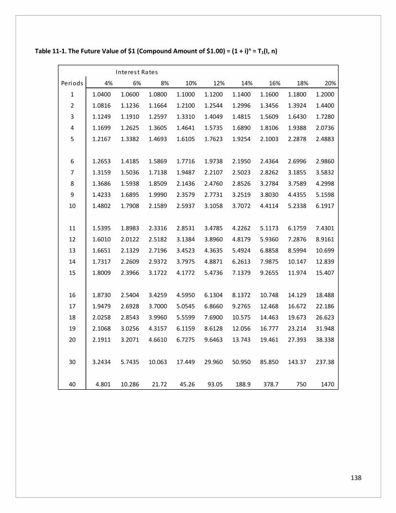
138

Table 11-1. The Future Value of $1 (Compound Amount of $1.00) = (1 + i)n = T1(I, n)

Interest Rates

Periods 4% 6% 8% 10% 12% 14% 16% 18% 20%

1 1.0400 1.0600 1.0800 1.1000 1.1200 1.1400 1.1600 1.1800 1.2000

2 1.0816 1.1236 1.1664 1.2100 1.2544 1.2996 1.3456 1.3924 1.4400

3 1.1249 1.1910 1.2597 1.3310 1.4049 1.4815 1.5609 1.6430 1.7280

4 1.1699 1.2625 1.3605 1.4641 1.5735 1.6890 1.8106 1.9388 2.0736

5 1.2167 1.3382 1.4693 1.6105 1.7623 1.9254 2.1003 2.2878 2.4883

6 1.2653 1.4185 1.5869 1.7716 1.9738 2.1950 2.4364 2.6996 2.9860

7 1.3159 1.5036 1.7138 1.9487 2.2107 2.5023 2.8262 3.1855 3.5832

8 1.3686 1.5938 1.8509 2.1436 2.4760 2.8526 3.2784 3.7589 4.2998

9 1.4233 1.6895 1.9990 2.3579 2.7731 3.2519 3.8030 4.4355 5.1598

10 1.4802 1.7908 2.1589 2.5937 3.1058 3.7072 4.4114 5.2338 6.1917

11 1.5395 1.8983 2.3316 2.8531 3.4785 4.2262 5.1173 6.1759 7.4301

12 1.6010 2.0122 2.5182 3.1384 3.8960 4.8179 5.9360 7.2876 8.9161

13 1.6651 2.1329 2.7196 3.4523 4.3635 5.4924 6.8858 8.5994 10.699

14 1.7317 2.2609 2.9372 3.7975 4.8871 6.2613 7.9875 10.147 12.839

15 1.8009 2.3966 3.1722 4.1772 5.4736 7.1379 9.2655 11.974 15.407

16 1.8730 2.5404 3.4259 4.5950 6.1304 8.1372 10.748 14.129 18.488

17 1.9479 2.6928 3.7000 5.0545 6.8660 9.2765 12.468 16.672 22.186

18 2.0258 2.8543 3.9960 5.5599 7.6900 10.575 14.463 19.673 26.623

19 2.1068 3.0256 4.3157 6.1159 8.6128 12.056 16.777 23.214 31.948

20 2.1911 3.2071 4.6610 6.7275 9.6463 13.743 19.461 27.393 38.338

30 3.2434 5.7435 10.063 17.449 29.960 50.950 85.850 143.37 237.38

40 4.801 10.286 21.72 45.26 93.05 188.9 378.7 750 1470

139

Table 11-2. The Future Value of an Annuity of $1 (Compound Amount of an Annuity of $1) = T2(i,n)

Interest Rates

Periods 4% 6% 8% 10% 12% 14% 16% 18% 20%

1 1.0000 1.0000 1.0000 1.0000 1.0000 1.0000 1.0000 1.0000 1.0000

2 2.0400 2.0600 2.0800 2.1000 2.1200 2.1400 2.1600 2.1800 2.2000

3 3.1216 3.1836 3.2464 3.3100 3.3744 3.4396 3.5056 3.5724 3.6400

4 4.2465 4.3746 4.5061 4.6410 4.7793 4.9211 5.0665 5.2154 5.3680

5 5.4163 5.6371 5.8666 6.1051 6.3528 6.6101 6.8771 7.1542 7.4416

6 6.6330 6.9753 7.3359 7.7156 8.1152 8.5355 8.9775 9.4420 9.9299

7 7.8983 8.3938 8.9228 9.4872 10.089 10.7305 11.4139 12.1415 12.9159

8 9.2142 9.8975 10.6366 11.436 12.300 13.2328 14.2401 15.3270 16.4991

9 10.5828 11.4913 12.4876 13.579 14.776 16.0853 17.5185 19.0859 20.7989

10 12.0061 13.1808 14.4866 15.937 17.549 19.3373 21.3215 23.5213 25.9587

11 13.4864 14.9716 16.6455 18.531 20.655 23.0445 25.7329 28.7551 32.1504

12 15.0258 16.8699 18.9771 21.384 24.133 27.2707 30.8502 34.9311 39.5805

13 16.6268 18.8821 21.4953 24.523 28.029 32.0887 36.7862 42.2187 48.4966

14 18.2919 21.0151 24.2149 27.975 32.393 37.5811 43.6720 50.8180 59.1959

15 20.0236 23.2760 27.1521 31.772 37.280 43.8424 51.6595 60.9653 72.0351

16 21.8245 25.6725 30.3243 35.950 42.753 50.9804 60.9250 72.9390 87.4421

17 23.6975 28.2129 33.7502 40.545 48.884 59.1176 71.6730 87.0680 105.931

18 25.6454 30.9057 37.4502 45.599 55.750 68.3941 84.1407 103.740 128.117

19 27.6712 33.7600 41.4463 51.159 63.440 78.9692 98.6032 123.414 154.740

20 29.7781 36.7856 45.7620 57.275 72.052 91.0249 115.380 146.628 186.688

30 56.0849 79.0582 113.283 164.494 241.333 356.787 530.312 790.948 1181.88

40 95.026 154.762 259.06 442.59 767.09 1342.0 2360.8 4163 7344

140

Table 11-3. The Present Value of $1 = T3 (i,n)

Interest Rates

Periods 4% 6% 8% 10% 12% 14% 16% 18% 20%

1 0.9615 0.9434 0.9259 0.9091 0.8929 0.8772 0.8621 0.8475 0.8333

2 0.9246 0.8900 0.8573 0.8264 0.7972 0.7695 0.7432 0.7182 0.6944

3 0.8890 0.8396 0.7938 0.7513 0.7118 0.6750 0.6407 0.6086 0.5787

4 0.8548 0.7921 0.7350 0.6830 0.6355 0.5921 0.5523 0.5158 0.4823

5 0.8219 0.7473 0.6806 0.6209 0.5674 0.5194 0.4761 0.4371 0.4019

6 0.7903 0.7050 0.6302 0.5645 0.5066 0.4556 0.4104 0.3704 0.3349

7 0.7599 0.6651 0.5835 0.5132 0.4523 0.3996 0.3538 0.3139 0.2791

8 0.7307 0.6274 0.5403 0.4665 0.4039 0.3506 0.3050 0.2660 0.2326

9 0.7026 0.5919 0.5002 0.4241 0.3606 0.3075 0.2630 0.2255 0.1938

10 0.6756 0.5584 0.4632 0.3855 0.3220 0.2697 0.2267 0.1911 0.1615

11 0.6496 0.5268 0.4289 0.3505 0.2875 0.2366 0.1954 0.1619 0.1346

12 0.6246 0.4970 0.3971 0.3186 0.2567 0.2076 0.1685 0.1372 0.1122

13 0.6006 0.4688 0.3677 0.2897 0.2292 0.1821 0.1452 0.1163 0.0935

14 0.5775 0.4423 0.3405 0.2633 0.2046 0.1597 0.1252 0.0985 0.0779

15 0.5553 0.4173 0.3152 0.2394 0.1827 0.1401 0.1079 0.0835 0.0649

16 0.5339 0.3936 0.2919 0.2176 0.1631 0.1229 0.0930 0.0708 0.0541

17 0.5134 0.3714 0.2703 0.1978 0.1456 0.1078 0.0802 0.0600 0.0451

18 0.4936 0.3503 0.2502 0.1799 0.1300 0.0946 0.0691 0.0508 0.0376

19 0.4746 0.3305 0.2317 0.1635 0.1161 0.0829 0.0596 0.0431 0.0313

20 0.4564 0.3118 0.2145 0.1486 0.1037 0.0728 0.0514 0.0365 0.0261

30 0.3083 0.1741 0.0994 0.0573 0.0334 0.0196 0.0116 0.0070 0.0042

40 0.2083 0.0972 0.0460 0.0221 0.0107 0.0053 0.0026 0.0013 0.0007

141

Table 11-4. The Present Value of an Annuity of $1 = T4(i,n)

Interest Rates

Periods 4% 6% 8% 10% 12% 14% 16% 18% 20%

1 0.9615 0.9434 0.9259 0.9091 0.8929 0.8772 0.8621 0.8475 0.8333

2 1.8861 1.8334 1.7833 1.7355 1.6901 1.6467 1.6052 1.5656 1.5278

3 2.7751 2.6730 2.5771 2.4869 2.4018 2.3216 2.2459 2.1743 2.1065

4 3.6299 3.4651 3.3121 3.1699 3.0373 2.9137 2.7982 2.6901 2.5887

5 4.4518 4.2124 3.9927 3.7908 3.6048 3.4331 3.2743 3.1272 2.9906

6 5.2421 4.9173 4.6229 4.3553 4.1114 3.8887 3.6847 3.4976 3.3255

7 6.0021 5.5824 5.2064 4.8684 4.5638 4.2883 4.0386 3.8115 3.6046

8 6.7327 6.2098 5.7466 5.3349 4.9676 4.6389 4.3436 4.0776 3.8372

9 7.4353 6.8017 6.2469 5.7590 5.3282 4.9464 4.6065 4.3030 4.0310

10 8.1109 7.3601 6.7101 6.1446 5.6502 5.2161 4.8332 4.4941 4.1925

11 8.7605 7.8869 7.1390 6.4951 5.9377 5.4527 5.0286 4.6560 4.3271

12 9.3851 8.3838 7.5361 6.8137 6.1944 5.6603 5.1971 4.7932 4.4392

13 9.9856 8.8527 7.9038 7.1034 6.4235 5.8424 5.3423 4.9095 4.5327

14 10.5631 9.2950 8.2442 7.3667 6.6282 6.0021 5.4675 5.0081 4.6106

15 11.1184 9.7122 8.5595 7.6061 6.8109 6.1422 5.5755 5.0916 4.6755

16 11.6523 10.1059 8.8514 7.8237 6.9740 6.2651 5.6685 5.1624 4.7296

17 12.1657 10.4773 9.1216 8.0216 7.1196 6.3729 5.7487 5.2223 4.7746

18 12.6593 10.8276 9.3719 8.2014 7.2497 6.4674 5.8178 5.2732 4.8122

19 13.1339 11.1581 9.6036 8.3649 7.3658 6.5504 5.8775 5.3162 4.8435

20 13.5903 11.4699 9.8181 8.5136 7.4694 6.6231 5.9288 5.3527 4.8696

30 17.2920 13.7648 11.2578 9.4269 8.0552 7.0027 6.1772 5.5168 4.9789

40 19.7928 15.0463 11.9246 9.7791 8.2438 7.1050 6.2335 5.5482 4.9966

142


1. John Watson's uncle recently passed away and included in the property that John inherited is a bond that pays

an 8% coupon, has a face value of $1,000, has 10 years to maturity, and the investors require a rate of return of

10%. Assuming annual coupon payments, what is the value of the bond?

A. $386.00

B. $491.60

C. $614.50

D. $877.60

2. On November 1, 20X5, a company purchased a new machine that it does not have to pay for until November 1,

20X7. The total payment on November 1, 20X7 will include both principal and interest. Assuming interest at a 10%

rate, the cost of the machine would be the total payment multiplied by what time value of money concept?

A. Present value of an annuity of $1

B. Present value of $1

C. Future amount of an annuity of $1

D. Future amount of $1

3. Pole Co. is investing in a machine with a 3-year life. The machine is expected to reduce annual cash operating

costs by $30,000 in each of the first 2 years and by $20,000 in year 3. Using a 14% cost of capital (discount rate),

what is the present value of these future savings? Note: The Present Values of $1 at 14% for period 1 = 0.88, for

period 2 = 0.77, and for period 3 = 0.68. The Present Values of an Annuity of $1 at 14% for period 1 = 0.88, for

period 2 = 1.65, and period 3 = 2.32. )

A. $59,600

B. $69,600

C. $63,100

D. $69,500

143

Chapter 12: Capital Investment Decisions

Learning Objectives


• Recognize each of the basic capital investment analysis techniques

• Recognize the various types of depreciation methods

There are many investment decisions that the company may have to make in order to grow. These decisions should

be made in light of the goals of the company. The stockholders have entrusted the company with their money and

they expect the firm to invest their money wisely. Investments in fixed assets should be consistent with the goal of

maximizing the market value of the firm.

Capital budgeting is the process of making long-term investment decisions. Examples of capital budgeting applications

are product line selection, keep or sell business-segment decisions, lease or buy decisions, and determination of which

asset to invest in. To make long-term investment decisions in accordance with its goal, you must perform three tasks

in evaluating capital budgeting projects:

• Estimate cash flows

• Estimate the cost of capital (or required rate of return)

• Apply a decision rule to determine if a project is "good" or "bad."

This chapter provides insights on evaluating long-term investment proposals with specific examples to illustrate

the application.

144

Investment Analysis Techniques

There are typically two types of long-term investment decisions made by your company:

1. Selection decisions in terms of obtaining new facilities or expanding existing facilities: Examples include:

a. Investments in property, plant, and equipment as well as other types of assets.

b. Resource commitments in the form of new product development, market research, information

technology (IT), refunding of long-term debt, etc.

c. Mergers and acquisitions in the form of buying another company to add a new product line.

2. Replacement decisions in terms of replacing existing facilities with new facilities. Examples include

replacing an old machine with a high-tech machine.

Long-term investments have three important features:

1. They typically involve a large amount of initial cash outlays that tend to have a long-term impact on the

firm's future profitability. Therefore, this initial cash outlay needs to be justified on a cost-benefit basis.

2. There are expected recurring cash inflows (for example, increased revenues, savings in cash operating

expenses, etc.) over the life of the investment project. This frequently requires considering the time value

of money.

3. Income taxes could make a difference in accept or reject decision. Therefore, income tax factors must be

taken into account in every capital budgeting decision.

Several methods of evaluating investment projects are as follows:

• Payback period

• Accounting rate of return (ARR)

• Net present value (NPV)

• Internal rate of return (IRR)

• Profitability index (or cost/benefit ratio)

The NPV method and the IRR method are called discounted cash flow (DCF) methods. Each of these methods is

discussed below.

Payback Period

The payback period measures the length of time required to recover the amount of initial investment. It is computed

by dividing the initial investment by the cash inflows through increased revenues or cost savings.

Examples 12-1 and 12-2 calculate the payback periods for two different situations.

145

EXAMPLE 12-1. Consider the following data:

Cost of investment $18,000

Annual after-tax cash savings $3,000

Then, the payback period is formulated as follows:

Payback period =

Decision rule: Choose the project with the shorter payback period. The rationale behind this choice is: The shorter

the payback period, the less risky the project, and the greater the liquidity.

EXAMPLE 12-2. Consider the two projects whose after-tax cash inflows are not even. Assume each project costs

$1,000.

Cash Inflows

Year A($) B($)

1 100 500

2 200 400

3 300 300

4 400 100

5 500

6 600

When cash inflows are not even, the payback period has to be found by trial and error. The payback period of

project A is ($1,000= $100 + $200 + $300 + $400) 4 years. The payback period of project B is $1,000 = $500 + $400 +

$100):

2 years +$100/$300 = 2-1/3 years

Project B is the project of choice in this case, since it has the shorter payback period.

The advantages of using the payback period method of evaluating an investment project are that (1) it is simple to

compute and easy to understand, and (2) it handles investment risk effectively. The shortcomings of this method are

that (1) it does not recognize the time value of money, and (2) it ignores the impact of cash inflows received after the

payback period; essentially, cash flows after the payback period determine the profitability of an investment.

Accounting Rate of Return

The accounting rate of return (ARR) measures profitability from the conventional accounting standpoint by relating

the required investment or sometimes the average investment to the future annual net income.

Decision rule: Under the ARR method, choose the project with the higher rate of return.

initial investment

cost savings years= =

$18,

$3,

000

0006

146

EXAMPLE 12-3. Consider the following investment:

Initial investment $6,500

Estimated life 20 years

Cash inflows per year $1,000

Depreciation per year (using straight-line method) $325

The accounting rate of return for this project is:

APR =

If average investment (usually assumed to be one-half of the original investment) is used, then:

APR =

The advantages of this method are that it is easily understandable, simple to compute, and recognizes the profitability

factor.

The shortcomings of this method are that it fails to recognize the time value of money, and it uses accounting data

instead of cash flow data.

Net Present Value

Net present value (NPV) is the excess of the present value (PV) of cash inflows generated by the project over the

amount of the initial investment (I):

NPV = PV - I

The present value of future cash flows is computed using the so-called cost of capital (or minimum required rate of

return) as the discount rate. In the case of an annuity, the present value would be

PV = A . T4 (i, n)

where A is the amount of the annuity. The value of T4 is found in Table 11-4.

Decision rule: If NPV is positive, accept the project. Otherwise, reject it.

net income

investment=

−=

$1000 $325

$6,.

50010 4%

$1, $325

$3,.

000

25020 8%

−=

147

EXAMPLE 12-4. Consider the following investment:

Initial investment $12,950

Estimated life 10 years

Annual cash inflows $3,000

Cost of capital (minimum required rate of return) 12%

Present value of the cash inflows is:

PV = A . T4 (i, n)

= $3,000 . T4 (12%,10 years)

= $3,000 (5.650) $16,950

Initial investment (I) 12,950

Net present value (NPV = PV - I) $ 4,000

Since the NPV of the investment is positive, the investment should be accepted.

The advantages of the NPV method are that it obviously recognizes the time value of money and it is easy to compute

whether the cash flows form an annuity or vary from period to period.

Internal Rate of Return

Internal rate of return (IRR) is defined as the rate of interest that equates I with the PV of future cash inflows. In other

words, at IRR,

I = PV

or

NPV = 0

Decision rule: Accept the project if the IRR exceeds the cost of capital. Otherwise, reject it.

EXAMPLE 12-5. Assume the same data given in Example 12-4, and set the following equality (I=PV):

$12,950 = $3,000 . T4(i,10 years)

T4(i,10 years) = $12,950/$3,000 = 4.317

which stands somewhere between 18 percent and 20 percent in the 10-year line of Table 11-4. The interpolation

follows:

PV of an Annuity of $1 Factor T4(i,10 years)

18% 4.494 4.495

IRR 4.317

20% 4.192

Difference 0.1777 0.302

148

Therefore,

IRR = 18% + (0.177/0.302) (20% - 18%)

= 18% + 0.586(2%) = 18% + 1.17% = 19.17%

Since the IRR of the investment is greater than the cost of capital (12 percent), accept the project.

Using Excel and the RATE function = RATE(nper,pmt,pv) =RATE(10,3000,-12950) = 19.1%

The advantage of using the IRR method is that it does consider the time value of money and, therefore, is more exact

and realistic than the ARR method. The shortcomings of this method are that:

• It can be time-consuming to compute, especially when the cash inflows are not even, although most

business calculators and spreadsheets have a program to calculate IRR.

• It fails to recognize the varying sizes of investment in competing projects.

When cash inflows are not even, IRR is computed by the trial and error method, which is not discussed here. Financial

calculators also have a key for IRR calculations.

Profitability Index

The profitability index is the ratio of the total PV of future cash inflows to the initial investment, that is, PV/I. This

index is used as a means of ranking projects in descending order of attractiveness.

Decision rule: If the profitability index is greater than 1, then accept the project.

EXAMPLE 12-6. Using the data in Example 12-4, the profitability index is

Since this project generates $1.31 for each dollar invested (i.e., its profitability index is greater than 1), accept the

project.

The profitability index has the advantage of putting all projects on the same relative basis regardless of size.

Many firms specify a limit on the overall budget for capital spending. Capital rationing is concerned with the problem

of selecting the mix of acceptable projects that provides the highest overall NPV. The profitability index is used widely

in ranking projects competing for limited funds.

PV

I= =

$16,

$12,.

950

950131

149

EXAMPLE 12-7. A company with a fixed budget of $250,000 needs to select a mix of acceptable projects from the

following:

Projects I($) PV($) NPV($) Profitability Index Ranking

A 70,000 112,000 42,000 1.6 1

B 100,000 145,000 45,000 1.45 2

C 110,000 126,500 16,500 1.15 5

D 60,000 79,000 19,000 1.32 3

E 40,000 38,000 -2,000 0.95 6

F 80,000 95,000 15,000 1.19 4

The ranking resulting from the profitability index shows that the company should select projects A, B, and D.

I PV

A $70,000 $112,000

B 100,000 145,000

D 60,000 79,000

230,000 $336,000

Therefore,

NPV = $336,000 - $230,000 = $106,000

The Effect of Income Taxes

Income taxes make a difference in many capital budgeting decisions. In other words, the project that is attractive on

a before-tax basis may have to be rejected on an after-tax basis. Income taxes typically affect both the amount and

the timing of cash flows. Since net income, not cash inflows, is subject to tax, after-tax cash inflows are not usually

the same as after-tax net income.

Let us define:

S = Sales

E = Cash operating expenses

d = Depreciation

t = Tax rate

Then, for a cash basis company whose book and tax depreciation are the same:

Before-tax cash inflows (or before-tax cash savings) = S - E

and net income = S - E - d.

By definition,

After-tax cash inflows = Before-tax cash inflows - Taxes

= (S - E) - (S - E - d) (t)

150

Stated another way: After-tax cash inflows = (S - E) (1 - t) + (d)(t)

A tax shield can be described as a reduction in income tax payments that result from taking allowable deductions

that reduce taxable income. The tax shield for depreciation is calculated as follows: As can be seen, the

deductibility of depreciation from sales in arriving at net income subject to taxes reduces income tax payments and

thus serves as a tax shield.

Tax shield = Tax savings on depreciation = (d)(t)

EXAMPLE 12-8. Assume:

S = $12,000

E = $10,000

d = $500 per year using the straight-line method

t = 30%

Then,

After-tax cash inflow = ($12,000 - $10,000) (1 - 0.3) + ($500)(0.3)

= ($2,000)(.7) + ($500)(0.3)

= $1,400 + $150 = $1,550

Note that the depreciation tax shield = tax savings on depreciation = (d)(t)

= ($500)(.3) = $150

Since the tax shield is dt, the higher the depreciation deduction, the higher the tax savings on depreciation will be.

Therefore, an accelerated depreciation method (such as double-declining balance) produces higher tax savings than

the straight-line method. Accelerated methods produce higher present values for the tax savings that may make a

given investment more attractive.

EXAMPLE 12-9. The Shalimar Company estimates that it can save $2,500 a year in cash operating costs for the next

ten years if it buys a special-purpose machine at a cost of $10,000. No salvage value is expected. Assume that the

income tax rate is 30%, and the after-tax cost of capital (minimum required rate of return) is 10%. After-tax cash

savings can be calculated as follows:

Note that depreciation by straight-line is $10,000/10 = $1,000 per year. Here before-tax cash savings = (S - E) = $2,500.

Thus,

After-tax cash savings = (S - E) (1 - t) + (d)(t)

= $2,500(1 - 0.3) + $1,000(0.3)

= $1,750 + $300 = $2,050

To see if this machine should be purchased, the net present value can be calculated.

PV = $2,050 T4(10%, 10 years) = $2,050 (6.145) = $12,597.25

Thus, NPV = PV - I = $12,597.25 - $10,000 = $2,597.25

Since NPV is positive, the machine should be purchased.

151

Depreciation Methods

We saw that depreciation provided the tax shield in the form of (d)(t). Among the commonly used depreciation

methods are straight-line and accelerated methods. The two major accelerated methods are sum-of-the years'-digits

(SYD) and double-declining-balance (DDB).

Straight-Line Method

This is the easiest and most popular method of calculating depreciation. It results in equal periodic depreciation

charges. The method is most appropriate when an asset's usage is uniform from period to period, as is the case with

furniture. The annual depreciation expense is calculated by using the following formula:

Depreciation expense = cost - salvage value

number of years of useful life

EXAMPLE 12-10. An auto is purchased for $20,000 and has an expected salvage value of $2,000. The auto's estimated

life is 8 years. Its annual depreciation is calculated as follows:

Depreciation expense = cost - salvage value

number of years of useful life

= ($20,000 - $2,000) / 8 years = $2,250 per year

An alternative means of computation is to multiply the depreciable cost ($18,000) by the annual depreciation rate,

which is 12.5 percent in this example. The annual rate is calculated by dividing the number of years of useful life into

one (1/8 = 12.5%). The result is the same: $18,000 x 12.5% = $2,250.

Sum-of-the-Years-Digits (SYD) Method

In this method, the number of years of life expectancy is enumerated in reverse order in the numerator, and the

denominator is the sum of the digits. For example, if the life expectancy of a machine is 8 years, write the numbers

in reverse order: 8, 7, 6, 5, 4, 3, 2, 1. The sum of these digits is 36, or (8 + 7 + 6 + 5 + 4 + 3 + 2 + 1). Thus, the fraction

for the first year is 8/36, while the fraction for the last year is 1/36. The sum of the eight fractions equals 36/36, or 1.

Therefore, at the end of 8 years, the machine is completely written down to its salvage value.

The following formula may be used to quickly find the sum-of-the-years' digits (S):

S = (N)(N +1)

2

152

where N represents the number of years of expected life.

EXAMPLE 12-11. In Example 12-10, the depreciable cost is $18,000 ($20,000 - $2,000). Using the SYD method, the

computation for each year's depreciation expense is

S =

Year Fraction x Depreciation = Depreciation Amount ($) Expense

1 8/36 $18,000 $4,000 2 7/36 18,000 3,500 3 6/36 18,000 3,000 4 5/36 18,000 2,500 5 4/36 18,000 2,000 6 3/36 18,000 1,500 7 2/36 18,000 1,000 8 1/36 18,000 500 Total $18,000

Double-Declining-Balance (DDB) Method

Under this method, depreciation expense is highest in the earlier years and lower in the later years. First, a

depreciation rate is determined by doubling the straight-line rate. For example, if an asset has a life of 10 years, the

straight-line rate is 1/10 or 10 percent, and the double-declining rate is 20 percent. Second, depreciation expense is

computed by multiplying the rate by the book value of the asset at the beginning of each year. Since book value

declines over time, the depreciation expense decreases each successive period.

This method ignores salvage value in the computation. However, the book value of the fixed asset at the end of its

useful life cannot be below its salvage value.

EXAMPLE 12-12. Assume the data in Example 12-10. Since the straight-line rate is 12.5 percent (1/8), the double-

declining-balance rate is 25 percent (2 x 12.5%). The depreciation expense is computed as follows:

Year Book Value at beginning of year

x Rate (%) = Depreciation Expense

Year-end Book Value

1 $20,000 25% $5,000 $15,000

2 15,000 25 3,750 11,250

3 11,250 25 2,813 8,437

4 8,437 25 2,109 6,328

5 6,328 25 1,582 4,746

6 4,746 25 1,187 3,559

7 3,559 25 890 2,669

8 2,669 25 667 2,002

362

72

2

)9(8

2

1)+(N)(N===

153

Note: If the original estimated salvage value had been $2,100, the depreciation expense for the eighth year would

have been $569 ($2,669 - $2,100) rather than $667 since the asset cannot be depreciated below its salvage value.

TABLE 12-1.

Selected MACRS Recovery Rates (rounded)

Based on the Property Classification of Assets (Half-Year Convention)

Year 3-year 5-year 7-year 10-year 15-year 20-year

1 33.3% 20.0% 14.3% 10.0% 5.0% 3.8%

2 44.5 32.0 24.5 18.0 9.5 7.2

3 14.8a 19.2 17.5 14.4 8.6 6.7

4 7.4 11.5a 12.5 11.5 7.7 6.2

5 11.5 8.9a 9.2 6.9 5.7

6 5.8 8.9 7.4 6.2 5.3

7 8.9 6.6a 5.9a 4.9

8 4.5 6.6 5.9 4.5a

9 6.5 5.9 4.5

10 6.5 5.9 4.5

11 3.3 5.9 4.5

12 5.9 4.5

13 5.9 4.5

14 5.9 4.5

15 5.9 4.5

16 3.0 4.4

17 4.4

18 4.4

19 4.4

20 4.4

21 ____ ____ ____ ____ ____ 2.2

Total 100% 100% 100% 100% 100% 100%

a. Denotes the year of changeover to straight-line depreciation.

Modified Accelerated Cost Recovery System

In 1981 new method of computing depreciation deductions for tax purposes was introduced. The current rule is

called the Modified Accelerated Cost Recovery System (MACRS) rule, enacted by Congress in 1981 and then

modified somewhat in 1986 under the Tax Reform Act of 1986. This rule is characterized as follows:

1. It abandons the concept of useful life and accelerates depreciation deductions by placing all depreciable

assets into one of eight age property classes. It calculates deductions, based on an allowable percentage of

154

the asset's original cost over a specified recovery period (See Tables 12-1 and 12-2). Since the recovery period

is generally shorter than the useful life, the company would be able to deduct depreciation more quickly and

save more in income taxes in the earlier years, thereby making an investment more attractive. The rationale

behind the system is that this way the government encourages the company to invest in facilities and increase

its productive capacity and efficiency. (Remember that the higher d, the larger the tax shield (d)(t)).

2. Since the allowable percentages in Table 12-2 add up to 100%, there is no need to consider the salvage value

of an asset in computing depreciation.

3. The company may elect the straight-line method. The straight-line convention must follow what is called the

half-year convention unless the mid-quarter convention applies. This means that the company can deduct

only half of the regular straight-line depreciation amount in the first year. The reason for electing to use the

MACRS optional straight-line method is that some firms may prefer to have lower depreciation deductions in

the early years rather than to accelerate them. Those firms are generally just starting out or have little or no

income and/or wish to show more income on their income statements in the early years.

TABLE 12-2

MACRS TABLES BY PROPERTY CLASS

MACRS Property Class &

Depreciation Method

Useful Life

(ADR Midpoint Life) Examples of Assets

3-year property 200% declining

balance

4 years or less Most small tools and tractor units for use

over-the-road are included; the law

specifically excludes autos and light trucks

from this property class.


balance

More than 4 years to Less

than 10 years

Autos, computers and their peripheral

equipment, copiers, duplicating equipment,

and property used in experimentation and

research.


balance

10 years or more to less than

16 years

Office furniture and fixtures and most items

of machinery and equipment used in

production


balance


20 years

Various machinery and equipment, such as

that used in petroleum distilling and refining

and in the milling of grain, are included.


balance


25 years

Sewage treatment plants telephone and

electrical distribution facilities, and land

improvements such as shrubbery, fences and

sidewalks.


balance

25 years or more Service stations and other real property with

an ADR midpoint life of less than 27.5 years

are included.

155

27.5-year property straight-line Not applicable All residential rental property is included.

31.5 and 39-year property

straight-line

Not applicable All nonresidential real property is included.

“a” The term ADR midpoint life means the “useful life” of an asset in a business sense; the appropriate ADR

midpoint lives for assets are designated in the tax Regulations.

EXAMPLE 12-13. Assume that a machine falls under a 3-year property class and costs $3,000 initially. The straight-line

option under MACRS differs from the traditional straight-line method in that under this method the company would

deduct only $500 depreciation in the first and fourth years ($3,000/3 years =$1,000; $1,000/2=$500). The table below

compares the straight line with half-year convention with the MACRS.

Straight line

(half-year) MACRS

Year Depreciation Cost MACRS % Deduction

1 $ 500 $3,000 x 33.3% $ 999

2 1,000 3,000 x 44.5 1,335

3 1,000 3,000 x 14.8 444

4 500 3,000 x 7.4 222

$3,000 $3,000

EXAMPLE 12-14. A machine costs $1,000. Annual cash inflows are expected to be $500. The machine will be

depreciated using the MACRS rule and will fall under the 3-year property class. The cost of capital after taxes is 10%.

The estimated life of the machine is 4 years. The tax rate is 30%. The formula for computation of after-tax cash inflows

(S - E)(1 - t)+ (d)(t) needs to be computed separately. The NPV analysis can be performed as follows:

Present Value factor @ Present

10% value

3.170(a) $1,109.5

Year Cost MACRS% d (d)(t)

1 $1,000 x 33.3% $333 $99.9 .909(b) 90.81

2 $1,000 x 44.5 445 133.5 .826(b) 110.27

3 $1,000 x 14.8 148 44.4 .751(b) 33.34

4 $1,000 x 7.4 74 22.2 .683(b) 15.16

$1,359.08

(a) T4(10%, 4 years) = 3.170 (from Table 11-4).

(b) T3 values obtained from Table 11-3.

Therefore, NPV = PV - I = $1,359.08 - $1,000 = $359.08, which is positive, so that the machine should be bought.

(S - E)(1- t):

$500(1- 0.3) = $350 for 4 years

156

The Cost of Capital

The cost of capital is defined as the rate of return that is necessary to maintain the market value of the firm (or the

price of the firm's stock). Project managers must know the cost of capital, often called the minimum required rate of

return, in making capital budgeting decisions. It has been used either as a discount rate under the NPV method or as

a hurdle rate under the IRR method. The cost of capital is computed as a weighted average of the various capital

components, which are items on the right-hand side of the balance sheet such as debt, preferred stock, common

stock, and retained earnings described below.

The cost of debt is stated on an after-tax basis since the interest on the debt is tax-deductible. However, the cost of

preferred stock is the stated annual dividend rate. This rate is not adjusted for income taxes because the preferred

dividend, unlike debt interest, is not a deductible expense in computing corporate income taxes.

EXAMPLE 12-15. Assume that the Hume Company issues a $1,000, 8 percent, 20-year bond whose net proceeds

are $940. The tax rate is 40 percent. Then, the after-tax cost of debt is:

8.00% (1-0.4) = 4.8%

EXAMPLE 12-16. Suppose that the Hume company has preferred stock that pays a $12 dividend per share and sells

for $100 per share in the market. Then the cost of preferred stock is:

Dividend per share =

$12 = 12%

Price per share $100

The cost of common stock is generally viewed as the rate of return investors require on a firm's common stock. One

way to measure the cost of common stock is to use the Gordon's growth model. The model is

Po = D1

r - g

where

Po = value (or market price) of common stock

D1 = dividend to be received in 1 year

r = investor's required rate of return

g = rate of growth (assumed to be constant over time)

Solving the model for r results in the formula for the cost of common stock:

r = D1

+ g Po

157

EXAMPLE 12-17. Assume that the market price of the Hume Company's stock is $40. The dividend to be paid at

the end of the coming year is $4 per share and is expected to grow at a constant annual rate of 6 percent. Then

the cost of this common stock is:

D1 + g =

$4 + 6% = 16%

Po $40

The cost of retained earnings is closely related to the cost of existing common stock since the cost of equity obtained

by retained earnings is the same as the rate of return investors require on the firm's common stock.

The firm's overall cost of capital is the weighted average of the individual capital costs, with the weights being the

proportions of each type of capital used.

(percentage of the total capital structure supplied by each source of capital x cost of capital for each source)

The computation of the overall cost of capital is illustrated in the following example.

EXAMPLE 12-18. Assume that the capital structure at the latest statement date is indicative of the proportions of

financing that the company intends to use over time:

Cost

Bonds ($1,000 par) $20,000,000 4.80%

Preferred stock ($100 par) 5,000,000 12.00

Common stock ($40 par) 20,000,000 16.00

Retained earnings 5,000,000 16.00

Total $50,000,000

These proportions would be applied to the assumed individual explicit after-tax costs below:

Source Weights Cost Weighted Cost

Debt 40%(a) 4.80% 1.92%(b)

Preferred stock 10 12.00% 1.20

Common stock 40 16.00% 6.40

Retained earnings 10 16.00% 1.60

100% 11.12%

(a) $20,000,000/$50,000,000 = .40 = 40%

(b) 4.80% x 40% = 1.92%

The overall cost of capital is 11.12%

By computing a company's cost of capital, we can determine its minimum rate of return, which is used as the

discount rate in present value calculations and in calculating an investment center's residual income (RI). A

company's cost of capital is also an indicator of risk. For example, if your company's cost of financing increases, it

158

is being viewed as riskier by investors and creditors, who are demanding a higher return on their investments in

the form of higher dividend and interest rates.

Conclusion

We have examined the process of evaluating investment projects. We have also discussed five commonly used criteria

for evaluating capital budgeting projects, including the net present value (NPV) and internal rate of return (IRR)

methods. The problems that arise with mutually exclusive investments and capital rationing were addressed. Since

income taxes could make a difference in the accept or reject decision, tax factors must be taken into account in every

decision.

Although the traditional straight-line depreciation methods still can be used for computing depreciation for book

purposes, there are other methods of computing depreciation deductions for tax purposes. The rule is called the

accelerated cost recovery system (MACRS). It was enacted by Congress in 1981 and then modified somewhat in

1986 under the Tax Reform Act of 1986. We illustrated the use of MACRS and presented an overview of the

depreciation methods. We also covered how to calculate a firm’s cost of capital, which is used either as a discount

rate under the NPV method or as a hurdle rate under the IRR method earlier in the chapter and in calculating the

residual income (RI) in Chapter 13.

159


1. Doro Co. is considering the purchase of a $100,000 machine that is expected to result in a decrease of $25,000

per year in cash expenses after taxes. This machine, which has no residual value, has an estimated useful life of

10 years and will be depreciated on a straight-line basis. For this machine, what would the accounting rate of

return (ARR) based on initial investment be?

A. 10%

B. 15%

C. 25%

D. 35%

2. Neu Co. is considering the purchase of an investment that has a positive net present value (NPV) based on Neu's

12% hurdle rate (minimum required rate of return). What would the internal rate of return be?

A. 0

B. 12%

C. 12%

D. < 12%

160

Chapter 13: Managerial Performance Measures

Learning Objectives


• Recognize effects on the rate of return on investments (ROI)

• Identify the basic components of the Du Pont formula used to improve profit

The ability to measure managerial performance is essential in controlling operations toward the achievement of

organizational goals. As companies grow or their activities become more complex, they attempt to decentralize

decision making as much as possible. They do this by restructuring the firm into several divisions and treating each

as an independent business. The managers of these subunits or segments are then evaluated on the basis of the

effectiveness with which they use the assets entrusted to them. Managerial performance should ideally be

evaluated only on the basis of those factors controllable by the manager. Managers may control revenues, costs,

and/or investments in resources.

Perhaps the most widely used single measure of success of an organization and its subunits is the rate of return

on investment (ROI). Related is the return to stockholders, known as the return on equity (ROE). This chapter

covered in detail various strategies to increase the ROI.

What is Return on Investment

ROI relates net income to invested capital (total assets). ROI provides a standard for evaluating how efficiently

management employs the average dollar invested in a firm's assets, whether that dollar came from owners or

creditors. Furthermore, a better ROI can also translate directly into a higher return on the stockholders' equity.

ROI is calculated as:

ROI = Net profit after taxes

Total assets

161

EXAMPLE 13-1. Consider the following financial data:

Total assets = $100,000

Net profit after taxes = 18,000

Then, ROI = =

The problem with this formula is that it only tells you about how a company did and how well it fared in the

industry. It has very little value from the standpoint of profit planning.

ROI and the Du Pont Formula

ROI can be broken down into two factors: profit margin and asset turnover. In the past, managers have tended to

focus only on the profit margin earned and have ignored the turnover of assets. It is important to realize that

excessive funds tied up in assets can be just as much of a drag on profitability as excessive expenses.

The Du Pont Corporation was the first major company to recognize the importance of looking at both net profit

margin and total asset turnover in assessing the performance of an organization. The ROI breakdown, known as

the Du Pont formula, is expressed as a product of these two factors, as shown below.

ROI =

= (Net profit margin) x (Total asset turnover)

The Du Pont formula combines the income statement and balance sheet into this otherwise static measure of

performance. Net profit margin is a measure of profitability or operating efficiency. It is the percentage of profit

earned on sales. This percentage shows how many cents attach to each dollar of sales. On the other hand, total

asset turnover measures how well a company manages its assets. It is the number of times by which the

investment in assets turns over each year to generate sales.

The breakdown of ROI is based on the thesis that the profitability of a firm is directly related to management's

ability to manage assets efficiently and to control expenses effectively.

EXAMPLE 13-2. Assume the same data as in Example 13.1. Also, assume sales of $200,000.

Then, ROI = =

Net profit after taxes

Total assets

$18,

$100,

000

00018%=


Total assets


Sales

Sales

Total assets=


Total assets

$18,

$100,

000

00018%=

162

Alternatively,

Net profit margin = =

Total asset turnover =

Therefore,

ROI = Net profit margin x Total asset turnover = 9% x 2 times = 18%

The breakdown provides a lot of insights to financial managers on how to improve the profitability of the company

and investment strategy. (Note that net profit margin and total asset turnover are called hereafter margin and

turnover, respectively, for short). Specifically, it has several advantages over the original formula (i.e., net profit

after taxes/total assets) for profit planning. They are:

1. The importance of turnover as a key to the overall return on investment is emphasized in the breakdown.

In fact, turnover is just as important as the profit margin in enhancing overall return.

2. The importance of sales is explicitly recognized, which is not in the original formula.

3. The breakdown stresses the possibility of trading one for the other in an attempt to improve the overall

performance of a company. The margin and turnover complement each other. In other words, a low

turnover can be made up by a high margin, and vice versa.

EXAMPLE 13-3. The breakdown of ROI into its two components shows that a number of combinations of margin

and turnover can yield the same rate of return, as shown below:

Margin x Turnover = ROI

(1) 9% x 2 times = 18% (2) 8 x 2.25 = 18 (3) 6 x 3 = 18 (4) 4 x 4.5 = 18 (5) 3 x 6 = 18 (6) 2 x 9 = 18

The turnover-margin relationship and its resulting ROI are depicted in Figure 13-1. As the figure shows, the margin

and turnover factors complement each other. The weak margin can be complemented by a strong turnover and

vice versa. It also shows how important turnover is as a key to profit-making. In effect, these two factors are

equally important in overall profit performance.


Total assets

$18,

$200,

000

0009%=

Sales

Total assets2 times= =

$200,

$100,

000

000

163

Figure 13-1. The Margin-Turnover Relationship

Figure 13-1 can also be looked at as showing six companies that performed equally well (in terms of ROI), but with

varying income statements and balance sheets. There is no ROI that is satisfactory for all companies. Sound and

successful operation must point toward the optimum combination of profits, sales, and capital employed. The

combination will necessarily vary depending upon the nature of the business and the characteristics of the

product. An industry with products tailor-made to customers' specifications will have different margins and

turnover ratios, compared with industries that mass-produce highly competitive consumer goods. For example,

the combination (4) may describe a supermarket operation that inherently works with low margin and high

turnover, while the combination (1) may be a jewelry store that typically has a low turnover and high margin.

Profit Planning

The breakdown of ROI into margin and turnover gives management insight into planning for profit improvement

by revealing where weaknesses exist: margin or turnover, or both. Various actions can be taken to enhance ROI.

Generally, management can:

1. Improve margin

2. Improve turnover

3. Improve both

Alternative 1 demonstrates a popular way of improving performance. Margins may be increased by reducing

expenses, raising selling prices, or increasing sales faster than expenses. Some of the ways to reduce expenses

are:

1. Use less costly inputs of materials, although this can be dangerous in today's quality-oriented

environment.

2. Automate processes as much as possible to increase labor productivity. But this will probably increase

assets, thereby reducing turnover.

164

3. Bring the discretionary fixed costs under scrutiny, with various programs either curtailed or eliminated.

Discretionary fixed costs arise from annual budgeting decisions by management. Examples include

advertising, research and development, and management development programs. The cost-benefit

analysis is called for in order to justify the budgeted amount of each discretionary program.

A company with pricing power can raise selling prices and retain profitability without losing business. Pricing

power is the ability to raise prices even in poor economic times when unit sales volume may be flat and capacity

may not be fully utilized. It is also the ability to pass on cost increases to consumers without attracting domestic

and import competition, political opposition, regulation, new entrants, or threats of product substitution. The

company with pricing power must have a unique economic position. Companies that offer unique, high-quality

goods and services (where the service is more important than the cost) have this economic position.

Alternative 2 may be achieved by increasing sales while holding the investment in assets relatively constant, or

by reducing assets. Some of the strategies to reduce assets are:

1. Dispose of obsolete and redundant inventory. The computer has been extremely helpful in this regard,

making continuous monitoring of inventory more feasible for better control.

2. Devise various methods of speeding up the collection of receivables and also evaluate credit terms and

policies.

3. See if there are unused fixed assets.

4. Use the converted assets (primarily cash) obtained from the use of the previous methods to repay

outstanding debts or repurchase outstanding issues of stock. You may use those funds elsewhere to get

more profit, which will improve margin as well as turnover.

Alternative 3 may be achieved by increasing sales or by any combinations of alternatives 1 and 2.

Figure 13-2 shows complete details of the relationship of ROI to the underlying ratios -- margin and turnover --

and their components. This will help identify more detailed strategies to improve margin, turnover, or both.

EXAMPLE 13-4. Assume that management sets a 20% ROI as a profit target. It is currently making an 18 percent

return on its investment.

ROI =

Present situation:

18% =

The following are illustrative of the strategies which might be used (each strategy is independent of the other).

Alternative 1: Increase the margin while holding turnover constant. Pursuing this strategy would involve leaving

selling prices as they are and making every effort to increase efficiency so as to reduce expenses. By doing so,

expenses might be reduced by $2,000 without affecting sales and investment to yield a 20% target ROI, as follows:


Total assets


Sales

Sales

Total assets=

18 000

200 000

200 000

100 000

,

,

,

,

165

20% =

Alternative 2: Increase turnover by reducing investment in assets while holding net profit and sales constant.

Working capital might be reduced or some land might be sold, reducing investment in assets by $10,000 without

affecting sales and net income to yield the 20% target ROI as follows:

20% =

Alternative 3: Increase both margin and turnover by disposing of obsolete and redundant inventories or through

an active advertising campaign. For example, trimming down $5,000 worth of investment in inventories would

also reduce the inventory holding charge by $1,000. This strategy would increase ROI to 20%.

20% =

Excessive investment in assets is just as much of a drag on profitability as excessive expenses. In this case, cutting

unnecessary inventories also helps cut down expenses of carrying those inventories, so that both margin and

turnover are improved at the same time. In practice, alternative 3 is much more common than alternative 1 or 2.

Return on Equity

Generally, a better management performance (i.e., a high or above-average ROI) produces a higher return to

equity holders. However, even a poorly managed company that suffers from a below-average performance can

generate an above-average return on the stockholders' equity, simply called the return on equity (ROE). This is

because borrowed funds can magnify the returns that a company's profits represent to its stockholders.

Another version of the Du Pont formula called the modified Du Pont formula reflects this effect. The formula ties

together the ROI and the degree of financial leverage (use of borrowed funds). The financial leverage is measured

by the equity multiplier, which is the ratio of a company's total asset base to its equity investment, or, stated

another way, the ratio of how many dollars of assets held per dollar of stockholders' equity. It is calculated by

dividing total assets by stockholders' equity. This measurement gives an indication of how much of a company's

assets are financed by stockholders' equity and how much with borrowed funds.

20 000

200 000

200 000

100 000

,

,

,

,

18 000

200 000

200 000

90 000

,

,

,

,

19 000

200 000

200 000

95 000

,

,

,

,

166

The return on equity (ROE) is calculated as:

= ROI x Equity multiplier

Figure 13-2. Relationships of Factors Influencing ROI

ROE measures the returns earned on the owners' (both preferred and common stockholders') investment. The

use of the equity multiplier to convert the ROI to the ROE reflects the impact of the leverage (use of debt) on the

stockholders' return.

The equity multiplier =

ROENet profit after taxes

Stockholders' equity


Total assets

Total assets

Stockholders' equity= =

Total assets

Stockholders' equity

167

=

=

=

Figure 13-3 shows the relationship between ROI, ROE, and financial leverage.

Figure 13-3. ROI, ROE, and Financial Leverage

EXAMPLE 13-5. In Example 13-1, assume stockholders' equity of $45,000.

Then, equity multiplier =

=

Total assets

Total assets - Total liabilities

1

1-Total liabilities

Total assets

1

(1- debt ratio)

Total assets


$100,

$45,.

000

0002 22

1

(1- debt ratio)=

−= =

1

1 0 55

1

0 452 22

( . ) ..

168

ROE =

ROE = ROI x equity multiplier = 18% x 2.22 = 40%

If the company used only equity, the 18% ROI would equal ROE. However, 55% of the firm's capital is supplied by

creditors ($45,000/$100,000 =45% is the equity-to-asset ratio; $55,000/$100,000 = 55% is the debt ratio). Since

the 18% ROI all goes to stockholders, who put up only 45% of the capital, the ROE is higher than 18%. This example

indicates the company was using leverage (debt) favorably.

EXAMPLE 13-6. To further demonstrate the interrelationship between a firm's financial structure and the return

it generates on the stockholders' investments, let us compare two firms that generate $300,000 in operating

income. Both firms employ $800,000 in total assets, but they have different capital structures. One firm employs

no debt, whereas the other uses $400,000 in borrowed funds. The comparative capital structures are shown as:

A B

Total assets $800,000 $800,000

Total liabilities -- 400,000

Stockholders' equity(a) 800,000 400,000


stockholders' equity $800,000 $800,000

Firm B pays 10% interest for borrowed funds. The comparative income statements and ROEs for firms A and B

would look as follows:

Operating income $300,000 $300,000

Interest expense - (40,000)

Profit before taxes $300,000 $260,000

Taxes (30% assumed) (90,000) (78,000)

Net Profit after taxes (b) $210,000 $182,000

ROE [(b)/(a)] 26.25% 45.5%

The absence of debt allows firm A to register higher profits after taxes. Yet the owners in firm B enjoy a significantly

higher return on their investments. This provides an important view of the positive contribution debt can make

to a business, but within a certain limit. Too much debt can increase the firm's financial risk and thus the cost of

financing.

If the assets in which the funds are invested are able to earn a return greater than the fixed rate of return required

by the creditors, the leverage is positive and the common stockholders benefit. The advantage of this formula is

that it enables the company to break its ROE into a profit margin portion (net profit margin), an

efficiency-of-asset-utilization portion (total asset turnover), and a use-of-leverage portion (equity multiplier). It



$18,

$45,

000

00040%

169

shows that the company can raise shareholder return by employing leverage - taking on larger amounts of debt

to help finance growth.

Since financial leverage affects net profit margin through the added interest costs, management must look at the

various pieces of this ROE equation, within the context of the whole, to earn the highest return for stockholders.

Financial managers have the task of determining just what combination of asset return and leverage will work

best in its competitive environment. Most companies try to keep at least a level equal to what is considered to be

"normal" within the industry.

Unfortunately, leverage is a two-edged sword. If assets are unable to earn a high enough rate to cover fixed

finance charges, then stockholders suffer. The reason is that part of the profits from the assets which the

stockholder has provided to the firm will have to go to make up the shortfall to the long-term creditors, and he/she

will be left with a smaller return than otherwise have been earned.

Conclusion

The breakdown of ROI into margin and turnover, popularly known as the Du Pont formula, provides lots of insight

into: (a) the strengths and weaknesses of a business and its segments, and (b) what needs to be done in order to

improve performance. Another version of the Du Pont formula --the modified Du Pont formula-- relates ROI to

ROE (stockholders' return) through financial leverage. It shows how leverage can work favorably for the owners

of the company.

170


1. Which combination of changes in asset turnover and profit margin on sales will maximize the return on

investment?

A. Increase asset turnover, and decrease profit margin

B. Increase asset turnover, and increase profit margin

C. Decrease asset turnover, and increase profit margin

D. Decrease asset turnover, and decrease profit margin

2. Return on investment (ROI) may be calculated by dividing net profit after taxes by debt ratios. True or False?

3. Return on investment (ROI) may be calculated by multiplying net profit margin by equity. True or False?

4. An investor has been given several financial ratios for a firm but none of the financial reports. Which

combination of ratios can be used to derive return on equity?

A. Market-to-book-value ratio and total-debt-to-total-assets ratio.

B. Net profit margin, total assets turnover, and equity multiplier.

C. Price-to-earnings ratio, earnings per share, and net profit margin.

D. Price-to-earnings ratio and return-on-assets ratio.

5. The following ratios relate to a company’s financial situation compared with that of its industry: The company

has an ROI = 7.9% and an ROE = 15.2%. The industry has an ROI = 9.2% and an ROE = 12.9%. What conclusion

could a financial analyst validly draw from these ratios?

A. The company's product has a high market share, leading to higher profitability.

B. The company uses more debt than does the average company in the industry.

C. The company's profits are increasing over time.

D. The company's shares have a higher market value to carrying amount than does the rest of the industry.

171

Chapter 14: Segmental Performance Measures

Learning Objectives


• Recognize the types of responsibility centers

• Identify the value of transfer pricing

In the previous chapter, we discussed how to analyze and evaluate managerial performance. We touched on a

broad measure of performance-that is, return on investment (ROI). In this chapter, we will focus on the

performance of a segment within a firm. The ability to measure performance is essential in developing

management incentives and controlling the operation toward the achievement of organizational goals. You

should know the financial strengths and weaknesses of your responsibility center, and what actions you should

take, if any, to improve performance.

Use of Segmental Analysis

A segment is a part or activity of a company for which a manager desires cost or revenue data. Examples of

segments are divisions, sales territories, individual stores, service centers, manufacturing plants, sales

departments, product lines, distribution channels, processes, programs, geographic areas, types of customers,

jobs, and contracts. Segmental reports may be prepared for activity at different levels within your responsibility

center and in varying formats, depending on your needs.

Segmental reporting reveals your department's performance. It also shows whether or not your product lines are

profitable. Segment reports will help you determine what types of goods are being bought by your customers,

what profit you are earning from each customer, which sales territories have a poor sales mix, whether or not

your salespeople are doing a good job, and whether or not production workers are performing effectively.

Analysis of segmental performance helps you evaluate the success or failure of your segment. For example,

divisional performance measures are concerned with the contribution of the division to profit and quality as well

as whether or not the division meets overall goals.

172

In evaluating a product line, consideration should be given to profitability, growth, competition, and capital

employed, you will have to determine whether to drop unprofitable products or substantially raise prices.

Within a customer class, there may also be a difference in selling costs to different customers within that class.

Why? Perhaps some customers need more extensive services (e.g., delivery, warehousing). Customer analysis

will show the difference in profitability among customers so that corrective action may be taken. The analysis will

aid in formulating selling prices and monitoring and controlling distribution costs. It will help you determine the

impact on the profitability of proposed price and volume changes.

In appraising your performance as the manager of the segment, you must determine which factors were under

your control (e.g., advertising budget) and which factors were not (e.g., economic conditions). The comparison

should be made of the performance of your division to other divisions in the company as well as to similar divisions

in competing companies. An appraisal should also be made of the risk and earning potential of your division.

The reasons to measure your performance as a division manager are as follows:

• It assists in formulating incentives and controlling operations to meet company and departmental goals.

• It points to trouble spots needing attention.

• It helps you determine who should be rewarded for good performance.

• It helps you determine who is not doing well so that corrective action may be taken.

• It aids in allocating time among projects.

• It provides job satisfaction since you receive feedback.

Responsibility Centers

Responsibility accounting is the system for collecting and reporting revenue and cost information by areas of

responsibility. It operates on the premise that you should be held responsible for your performance, the

performance of your subordinates, and for all activities within your responsibility center. It is both a planning and

control technique.

Responsibility accounting:

1. Facilitates delegation of decision making

2. Helps promote "management by objective," in which managers agree on a set of goals (your performance

is evaluated based on the attainment of these goals)

3. Permits effective use of "management by exception."

A responsibility center is a unit that has control over costs, revenues, and investment funds. This center may be

responsible for all three functions or for only one function. Divisional performance is analyzed by responsibility

center, which is comprised of a:

1. Revenue center

2. Cost center

173

3. Profit center

4. Investment center

5. Each type of responsibility center is discussed in the following sections.

Responsibility centers are found in both centralized and decentralized organizations. A profit center is often

associated with a decentralized organization, while a cost center is usually associated with a centralized one.

Responsibility centers are lines of responsibility within a company. Exxon-Mobil, for example, is organized

primarily by business functions: exploitation, refining, and marketing. General Foods, on the other hand, is

organized by product lines. To understand these lines, you should know how your company is organized. Figure

14-1 shows responsibility centers within an organization, while Figure 14-2 presents an organization chart of a

company.

Figure 14-1. Responsibility Centers within a Company

174

Figure 14-2. Organization Chart of a Company

Revenue Center

As the manager of a revenue center, you are responsible for obtaining a target level of sales revenue. An example

is a district sales office. The performance report contains the budgeted and actual sales for the center by product,

including evaluation. Usually, you are responsible for marketing a product line. But a revenue center typically has

a few costs (e.g., salaries, rent). Hence, you are responsible mostly for revenues and only incidentally for some

costs (typically not product costs). Accountability for departmental sales revenue also assumes that you have the

authority to determine product sales prices.

If you are to generate profitable sales, you must know what areas have the greatest profitability. This requires

sound sales analysis and cost evaluation. Sales analysis may involve one or more of the following: prior sales

performance, looking at sales trends over the years, and comparing actual sales to budgeted sales. Analyses may

be in dollars and/or units. The types of analysis include by salesperson, terms of sale, order size, channel of

distribution, customer, product, and territory. Sub-analyses may also be made for evaluating product sales in

each territory.

Sales analyses can help you uncover unwanted situations, such as when most of your division's sales are derived

from a small share of your product line. Further, you may see that only a few customers give you most of your

sales volume. Thus, a small part of the selling effort is needed for a high percentage of your business. After

studying the information, you may more narrowly focus your sales effort, resulting in fewer selling expenses.

Territorial assignments may be changed, or the product line may be simplified.

Sales analysis will also allow you to see if sales effort is directed toward the wrong products and if sales of products

are going toward less profitable lines. In appraising sales effort, consideration should be given to the number of

calls, ads placed, and mailings, and their results.

You should keep a record of sales levels for the same product at varying prices so as to establish a relationship of

volume to price.

175

Also, sales orders and backorders may be used as measures of projected volume. You can determine whether

orders have been lost by stockouts or delayed shipments.

Cost Center

A cost center is typically the smallest segment of activity or responsibility for cost accumulation. Examples of cost

centers include the maintenance department or the fabricating department in a manufacturing company. Cost

centers may be relatively small - a single department with few employees - or very large such as an administrative

area of a large company or an entire factory. Some cost centers may be comprised of smaller cost centers. For

instance, a factory may be segmented into numerous departments, each of which is a cost center. Generally, cost

centers pertain more to departments than to divisions.

A cost center manager is responsible for direct operational costs and for meeting production budgets and quotas.

The cost center manager, usually a department head, carries the authority and responsibility for costs and for

quantity and quality of not only products but services as well. For example, the personnel manager oversees both

the costs and the quality of services rendered. Managers of cost centers, however, have no control over sales or

marketing activities. Departmental profit is difficult to derive because of problems in allocating revenue and costs.

With a cost center, you must compare budgeted cost to actual cost. Variances are investigated to determine the

reasons for particular costs, necessary corrective action is taken to correct problems, and efficiencies are accorded

recognition. The cost center approach is useful when you possess control over your costs at a specific operating

level.

You may use the cost center approach when problems arise in relating financial measures to output. Cost center

evaluation is most suitable for the following functions, where problems in quantifying the output in financial terms

occur: accounting and financial reporting, legal, computer services, marketing, personnel, and public relations.

You will also find the cost center approach appropriate for nonprofit and governmental units where budgetary

appropriations are assigned. Actual expenditures are compared to budget. Your performance depends on your

ability to achieve output levels given budgetary constraints.

When looking at your performance, say at bonus time, the relevant costs are those incremental costs you have

control over. Incremental costs are those expenditures that would not exist if the center were abandoned. Hence,

allocated common costs (e.g., general administration) should not be included in appraising your performance.

Such costs should, however, be allocated in determining the profit for the division. Cost allocation must conform

to department goals and should be applied consistently among divisions.

Cost center evaluation will not be worthwhile unless reliable budget figures exist. If a division's situation

significantly changes, an adjustment to the initial budget is necessary. In such a case, the actual cost should be

compared with the initial budget figure (original goal) and the revised budget. Flexible budgets should be

prepared to enable you to look at costs at different levels of capacity. For example, you can budget figures for

expected capacity, optimistic capacity, and pessimistic capacity. Better comparisons of budget to actual can thus

be made given changing circumstances.

176

If you are a manager in the factory, you should consider factory performance measures such as yield percentages

for direct materials, number of rejects, capacity utilization, and cost per labor hour.

Provision should exist for chargebacks, where appropriate. For example, if the quality control department makes

an effort in its evaluation which leads to acceptance of the product by the purchasing department, the former

should be charged with the increased costs necessary to meet acceptable standards incurred by the purchasing

department.

When a transfer occurs between cost centers, the transfer price should be based on either actual cost, standard

cost, or controllable cost. Transfer price is the price charged between divisions for a product or service. Warning:

Using actual cost can pass cost inefficiencies onto the next division. There is no incentive to control costs.

Solution: Using standard cost solves this problem because the selling division will only be credited for what the

item should cost.

A good transfer price is a controllable cost. The cost center should be charged with actual controllable cost and

credited with standard controllable cost for the assembled product or service passed to other divisions. By

including just controllable cost, the subjectivity of the allocation of fixed non-controllable cost does not exist.

You should be aware of the effects of discretionary costs when evaluating performance. Discretionary costs are

those that can be easily changed such as advertising and research. A cutback in discretionary costs will produce

short-term improvements in profitability but in the long run, it will likely have a negative effect.

In evaluating administrative functions, performance reports should examine such dollar indicators as executive

salaries and service departments as well as ‘non-dollar’ measures such as the number of files handled, phone calls

taken, and invoices processed.

Profit Center

Profits can be expressed in several ways including net income, controllable margin, gross profit, controllable profit,

and incremental profit. A center thus measures the performance of a division, a product line, graphic area, or any

other quantifiable unit, using one of these expressions. On the other hand, profit centers have associated revenues

and expenses, and net income and contribution margin can be computed for them.

A typical profit center is a division selling a limited number of products or serving a particular geographic area.

The profit center provides goods and services but also the means for marketing them.

In some instances, profit centers are formed when products or services are used solely within the company. For

example, the computer department may be considered a profit center, as it bills each of the administrative and

operating units for services rendered.

A profit center demonstrates the following characteristics: (1) defined profit objective, (2) managerial authority

for making decisions that have an impact on earnings, and (3) the use of profit-oriented decision rules.

177

The profit center approach enhances decentralization and delineates units for decision-making purposes. It

should be used if your division is self-contained (with its own manufacturing and distribution facilities) and when

there are a limited number of interdivisional transfers. The reason is that the profit reported by the division is

basically independent of other divisions' operating activities, performance efficiencies, and managerial decisions.

Further, divisional earnings should not be increased by any action reducing overall corporate profitability. Also,

use the profit center approach when you have decision-making authority in terms of the quantity and mix of goods

or services. Because with a profit center, net income is determined as if the division were a separate economic

entity, you should be more cognizant of outside market considerations.

In using the profit center approach, it is not essential to allocate fixed costs. In general, fixed costs are much less

controllable than variable costs, which are common to a group of divisions. Hence, the contribution margin may

be a good indicator of your division's performance because it emphasizes cost behavior patterns and

controllability of costs that are generally useful for evaluating performance and making decisions. The

contribution margin approach aids in computing selling price, output levels, the price to accept an order given an

idle capacity situation, maximization of resource uses, and break-even analysis. Ultimately, if your division meets

its target contribution margin, any excess will be available to cover general corporate expenses.

To evaluate divisional and managerial performance, a contribution income statement can be prepared. Table 14-

1 presents a contribution margin income statement by division, with a further breakdown into product lines. Table

14-2 illustrates product line profitability.

Table 14-1. Contribution Margin Income Statement by Segments

Division Breakdown

Breakdown of Division Y Entire Product

Company X Y Unallocable 1 2 3 4 Sales $1,200 $300 $900 $300 $100 $200 $300 Less: Variable manufacturing cost of sales (700) (200) (500) (100) (50) (100) (250) Manufacturing contribution margin $500 $100 $400 $200 $50 $100 $50 Less: Variable selling and administrative costs (200) (50) (150) (40) (40) (40) (30) Contribution margin $300 $50 $250 $160 $10 $60 $20 Less: Controllable fixed costs by segment managers (180) (40) (140) (40) (30) (5) (50) (15) Contribution controllable by segment managers $120 $10 $110 (40) $130 $5 $10 $5 Less: Fixed costs controllable by others (70) (6) (64) (20) (20) (15) (5) (4) Segmental contribution $50 $4 $46 $(60) $110 $(10) $5 $1 Less: Unallocated costs (23) Net income $27

a Only those costs logically traceable to a product line should be allocated.

178

Table 14-2. Contribution by Products

Entire Company Product A Product B

Projected-Sales $100,000 $60,000 $40,000

Variable costs

Goods sold 30,000 109000 20,000

Marketing 5,000 4,000 1,000

Less: Total variable costs (35,000) (14,000) (21,000)

Contribution margin 65,000 46,000 19,000

Direct fixed costs

Production 4,000 2,000 2,000

Marketing 3,000 2,000 1,000

Less: Total direct fixed costs (7,000) (4,000) (3,000)

Profit contribution 58,000 42,000 16,000

Common fixed costs

Production 10,000

Marketing 8,000

Administrative and

general 5,000

Less: Total common costs (23,000)

Income before tax $35,000

A difficulty with the profit center approach is that profit is calculated after subtracting non-controllable costs or

costs not directly related to the divisional activity that have been arbitrarily allocated. The ensuing profit figure

may be erroneous. However, cost allocation is required, since divisions must incorporate non-divisional costs that

have to be met before the company will show a profit. Policies optimizing divisional earnings will likewise optimize

corporate earnings even before the allocation of non-divisional expenses.

It is important to recognize that, while an uncontrollable income statement item is included in appraising the

performance of a profit center, it should not be used in evaluating you. An example is the effect of foreign

exchange transaction gains and losses because you may have no control over it.

As a profit center manager, you are responsible for not only profit and loss items attributable directly to your

division but also costs incurred outside of the center (e.g., headquarters, other divisions) for which your center

will be billed directly.

Advantages of the profit center approach are that it creates competition in a decentralized company, provides

goal congruence between a division and the company, and aids performance evaluation. A drawback is that

profits can be manipulated since expenses may be shifted among periods. Examples of discretionary costs where

management has wide latitude are research and repairs. Also, this approach does not consider the total assets

employed in the division to obtain the profit.

179

Example 14-1. It is important to know at what point to sell an item in order to maximize profitability. You can sell

a product at its intermediate point in Division A for $170 or its final point in Division B at $260. The outlay cost in

Division A is $120, while the outlay cost in Division B is $110. Unlimited product demand exists for both the

intermediate product and the final product. Capacity is interchangeable. The divisional performance follows:

Division A Division B

Selling Price: $178 $260

Less: Outlay cost A (120) (120)

Outlay cost B (110)

Profit $ 50 $ 30

Sell at the intermediate point because of the higher profit.

Other measures in appraising divisional performance that are not of a profit nature but that must be considered

are the following:

• Ratios between cost elements and assets to appraise effectiveness and efficiency.

• Productivity measures, including input-output relationships. An example is labor hours in a production

run. You have to consider the input in time and money and the resulting output in quantity and quality.

Does the maintenance of equipment ensure future growth?

• Personnel development (e.g., number of promotions, turnover).

• Market measures (e.g., market share, product leadership, growth rate, customer service).

• Product leadership indicators (e.g., patented products, innovative technology, product quality, safety

record).

• Human resource relationships (e.g., employee turnover rate, customer relations, including on-time

deliveries).

• Social responsibility measures (e.g., consumer medals).

Investment Center

An investment center has control over revenue, cost, and investment funds. It is a profit center whose

performance is evaluated on the basis of the return earned on investment capital. An example is an auto product

line that is manufactured on company premises. Investment centers are widely used in highly diversified

companies.

A divisional investment is the amount placed in that division and put under your control. Two major divisional

performance indicators are return on investment (ROI) and residual income (RI). Assets assigned to a division

include direct assets in the division and allocated corporate assets. Assets are reflected at book value.

You should be able to distinguish between controllable and non-controllable investment. While the former is

helpful in appraising your performance, the latter is used to evaluate the entire division. Controllable investment

depends on the degree of your division's autonomy. As an investment center manager, you accept responsibility

for both the center's assets and the controllable income.

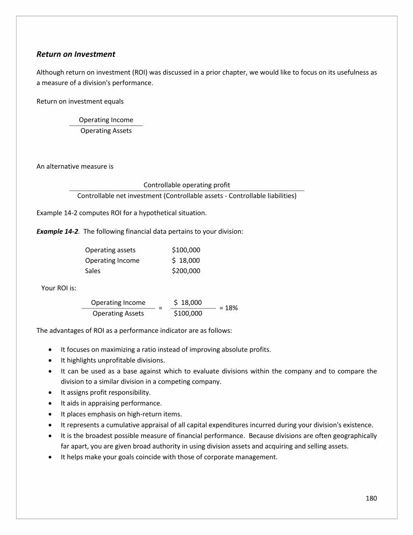
180

Return on Investment

Although return on investment (ROI) was discussed in a prior chapter, we would like to focus on its usefulness as

a measure of a division's performance.

Return on investment equals

Operating Income

Operating Assets

An alternative measure is

Controllable operating profit

Controllable net investment (Controllable assets - Controllable liabilities)

Example 14-2 computes ROI for a hypothetical situation.

Example 14-2. The following financial data pertains to your division:

Operating assets $100,000

Operating Income $ 18,000

Sales $200,000

Your ROI is:

Operating Income =

$ 18,000 = 18%

Operating Assets $100,000

The advantages of ROI as a performance indicator are as follows:

• It focuses on maximizing a ratio instead of improving absolute profits.

• It highlights unprofitable divisions.

• It can be used as a base against which to evaluate divisions within the company and to compare the

division to a similar division in a competing company.

• It assigns profit responsibility.

• It aids in appraising performance.

• It places emphasis on high-return items.

• It represents a cumulative appraisal of all capital expenditures incurred during your division's existence.

• It is the broadest possible measure of financial performance. Because divisions are often geographically

far apart, you are given broad authority in using division assets and acquiring and selling assets.

• It helps make your goals coincide with those of corporate management.

181

• It focuses on maximizing a ratio instead of improving absolute profits. Alternative profitability measures

could be used in the numerator besides net income (e.g., gross profit, contribution margin, segment

margin).

Disadvantages of ROI include:

• Different assets in the division must meet the same return rate regardless of the assets' riskiness.

• Established rate of return may be too high and could discourage incentive. A labor-intensive division

generally has a higher ROI than a capital-intensive one.

• ROI is a static indicator; it does not show future flows.

• A lack of goal congruence may exist between the company and your division. For example, if your

company’s ROI is 12%, your division's ROI is 18%, and a project's ROI is 16%, you will not accept the project

because it will lower your ROI, even though the project may be best for the entire company.

• ROI ignores risk.

• ROI emphasizes short-run performance instead of long-term profitability. To protect the current ROI, you

may be motivated to reject other profitable investment opportunities.

• If the projected ROI at the beginning of the year is set unrealistically high, discouragement of investment

center incentive could result.

An understanding of ROI enables you to see how your performance is measured and how your department

compares with other departments in the organization.

In an interview, a vice-president of a company commented on the usefulness of ROI in evaluating non-financial

managers:

“There are two department managers in separate areas with a goal of 15% ROI. Manager A decides that

to reach the goal he must increase the sales force by 15 agents. It takes six months to complete the

training, become fully functional, and contribute premium dollars. The training costs come to $60,000 per

agent, so we see that Manager A has invested heavily in human resources to increase income and affect

his ROI. Manager B decides to appeal to the existing sales force to increase their efficiency and production

with promises of no further hiring and encourages them to push the more profitable property lines.

Therefore, Manager B increases his department's ROI by increasing income while holding invested capital

steady.

You must evaluate these two managers one year later with regard to the company's goal of 15% ROI and

profitable growth. Without a full understanding of the implications and limitations of ROI, you decide that

Manager B has achieved his goals, while Manager A has only had his people functional for six months and

has not reached his 15% goal. However, being knowledgeable in accounting, you determine that Manager

B has merely opted to look good in the short term, but has actually jeopardized the company in the long

run by his failure to adequately forecast and plan accordingly. Manager B has not invested wisely in human

resources leaving you one year later with a sales force working to capacity with limited growth potential,

as they have saturated their markets and are not prepared to invade new markets. Manager A, on the

182

other hand, has increased his potential by investing wisely and now has 15 additional agents who are fully

trained and prepared to lead future company growth by expanding into untapped markets.

Taking a closer look at ROI reveals three added viewpoints. ROI can be positively affected by decreasing

costs, increasing revenue, or decreasing total assets. As a non-financial manager, you must be fully aware

of these factors so that you can evaluate your position accurately as each option presents its own set of

consequences. The proper use of accounting allows you to exercise the proper management controls,

along with allowing you to plan and monitor your financial. position as you move the organization towards

its goals.”

Residual Income

An alternative measure of divisional performance is residual income (RI), which equals divisional operating income

less minimum return times total operating assets.

Example 14-3. Divisional operating income is $250,000, total operating assets are $2 million, and the cost of

capital is 9%. Residual income equals

Divisional operating income $250,000

Less: Minimum x total operating assets

(9% x $2,000,000) (180,000)

Residual Income $70,000

The minimum return rate is based upon the company’s overall cost of financing adjusted for your division’s risk.

Residual income may be projected by division, center, or a specific program to ensure that the rate of return on

alternative investments is met or improved on by each segment. A target residual income may be formulated to

act as your objective. The trend in residual income to total available assets should be examined in appraising

divisional performance.

The advantages of residual income are as follows:

• The same asset may be required to earn the same return rate irrespective of the division the asset is in.

• Different return rates may be employed for different types of assets, depending on riskiness.

• Different return rates may be assigned to different divisions, depending on the risk of those divisions.

• RI provides an economic income, taking into account the opportunity cost of tying up assets in the division.

• RI identifies operating problem areas.

• RI maximizes dollars instead of a percentage, thereby motivating you to accept all profitable investments.

The disadvantages of residual income include the following:

• Assigning a minimum return involves estimating a risk level that is subjective.

• It may be difficult to determine the valuation basis and means of allocating assets to divisions.

183

• If book value is used in valuing assets, residual income will artificially increase over time, since the

minimum return times total assets becomes lower as the assets become older.

• RI cannot be used to compare divisions of different sizes. Residual income tends to favor the larger

divisions due to the larger amount of dollars involved.

• Since it is a mixture of controllable and uncontrollable elements, there is no segregation.

The decision of whether to use ROI or RI as a measure of your division's performance affects your investment

decisions. Under the ROI method, you tend to accept only the investments whose returns exceed the division's

ROI. Otherwise, the division's overall ROI would decrease if the investment were accepted. Under the RI method,

on the other hand, you would accept an investment as long as it earns a rate in excess of the minimum required

rate of return. The addition of such an investment will increase the division's overall RI.

Example 14-4. The following data apply to your division:

Operating assets $100,000

Operating Income $18,000

Minimum required rate of return 13%

ROI 18%

RI $5,000

Assume that you are presented with a project that would yield 15% on a $10,000 investment. You would not

accept this project under the ROI approach since the division is already earning 18%. Acquiring this project will

bring down the present ROI to 17.73%, as shown below:

Present New Project Overall

Operating assets (a) $100,000 $10,000 $110,000

Operating income (b) 18,000 1,500* 19,500

ROI (b/a) 18% 15% 17.73%

* $ 10,000 x 15% = $1,500

Under the RI approach, the manager would accept the new project because it provides a higher rate than the

minimum required rate of return (15% vs. 13%). Accepting the new project will increase the overall residual

income to $5,200, as shown below:

Present New Project Overall

Operating assets (a) $100,000 $10,000 $110,000

Operating income (b) 18,000 1,500 19,500

Less: Minimum required

income at 13% (c) (13,000) (1,300) * (14,300)

RI (b - c) $ 5,00 $200 $ 5,200

* $10,000 x 13% = $1,300

184

Transfer Pricing

The transfer price is the one credited to the selling division and charged to the buying division for an internal

transfer of an assembled product or service. The transfer resembles, for each division, an "arm’s length"

transaction. A transfer price has to be formulated so that a realistic and meaningful profit figure can be determined

for your division. It should be established after proper planning. Thus, you need to know what monetary values

to assign to these transfers—market prices, variable costs, full costs of some version of these values.

Unfortunately, there is no single transfer price that will please everybody--that is, top management, the selling

division, and the buying division involved in the transfer.

Transfer prices are not only important in performance, but also in decisions involving whether to make or buy,

whether to sell or process alternative production possibilities. Further, understanding the transfer pricing can

help account for possible cost overruns. You need to know what transfer price is being used for transfers and why

it is being used.

The best transfer price is the negotiated market value of the assembled product or service since it is a fair price

and treats each profit center as a separate economic entity. The negotiated market value equals the outside

service fee or selling price for the item (a quoted price for a product or service is only comparable if the credit

terms, grade, quality, delivery, and auxiliary conditions are precisely the same) less internal cost savings that result

from dealing within the organization (e.g., advertising, sales commission, delivery charges, credit and collections

costs).

The market value of services is based on the going rate for a specific job (e.g., equipment tune-up) and/or the

standard hourly rate (e.g., the hourly rate for an engineer). The market price may be determined from price the

Internet, catalogs, outside bids, and published data on complete market transactions. If two divisions cannot

agree on the transfer price, it may be settled by arbitration at a higher level. A temporarily low transfer price-

(e.g., due to oversupply of the item) or high transfer price (e.g., due to a strike situation causing a supply shortage)

should not be employed. An average long-term market price should be used.

A negotiated transfer price works best when outside markets for the intermediate product exist, all parties have

access to market information, and you are permitted to deal externally if a negotiated settlement is impossible.

If one of these conditions is violated, the negotiated price may break down and cause inefficiencies.

The negotiated market price can tell you whether an item should be produced internally or bought through an

outside vendor. If the cost of an item produced internally is more than the market price, you may want to go to

your superiors to suggest that the item no longer be supplied internally. You can suggest that the company buy

the item through a vendor, saving the company money overall. If the item is a by-product, this could tell

management that the cost of the materials is too high. This could make the purchasing department look for

another vendor. If the negotiated market value is too high, it could also show that the selling department is

wasting money.

185

If the outside market price is inappropriate or not ascertainable (e.g., new product, absence of replacement

market, or too costly to be used for transfer pricing), you should use budgeted cost plus profit markup because

this transfer price approximates market value and will highlight divisional inefficiencies. For example, if the

budgeted cost is $10 and a profit markup on cost of 20% is desired, the transfer price will be $12. Profit margin

should take into account the particular characteristics of your division (e.g., product line) rather than the overall

corporate profit margin.

There is an incentive to the selling division to control costs because it will not be credited for an amount exceeding

budgeted cost plus a markup. Thus, if the selling division's inefficiencies result in excessive actual costs, it would

have to absorb the decline in profit to the extent that actual cost exceeds budgeted cost.

Even though actual cost-plus profit markup may be used, it has the drawback of passing on cost inefficiencies. In

fact, the selling division is encouraged to be cost-inefficient, since the higher its actual cost is, the higher its selling

price (since it shows a greater profit) will be. Some division managers use actual cost as the transfer price because

of its ease of use, but the problem is that no profit is shown by the selling division and cost inefficiencies are

passed on. Further, the cost-based method treats the divisions as cost centers rather than profit or investment

centers. Therefore, measures such as return on investment and residual income cannot be used for evaluation

purposes.

A transfer price based on cost may be appropriate when minimal services are provided by your department to

another. If other departments provide identical or very similar services, a cost-based transfer price may be used

since the receiving department will select the services of the department providing the highest quality. Thus, the

providing department has an incentive to do a good job. A non-financial manager neatly illustrates this situation:

The two major areas of transfer pricing that directly affect my department are internal training and computer

equipment. Training, although internal, is also offered to the public. Because of this competitive situation,

training costs are charged to my department at the same amount as to outside companies. Computer equipment,

on the other hand, is sold (or leased) to my department at a discount over the price offered to the general public.

This is attributable to the fact that computer sales for the company have been rather sluggish, and the discount

offers an incentive to buy the company's brand over a competitor's.

We now see how transfer prices are used to determine divisional profit.

Example 14-5. Division A manufactures an assembled product that can be sold to outsiders or transferred to

Division B. Relevant information for the period follows:

Division A Units

Production 1,500

Transferred to Division B 1,200

Sold outside 300

Selling price $25

Unit cost $ 5

186

The units transferred to Division B were processed further at a cost of $7. They were sold outside at $45. Transfers

are at market value.

Division profit is computed as follows:

Division A Division B Company

Sales $ 7,500 $54,000 $61,500

Transfer price 30,000 _______ _______

$37,500 $54,000 $61,500

Product cost $ 7,500 $ 8,400 $15,900

Transfer price 30,000

($ 7,500) $38,400 $15,900

Profit $30,000 $15,600 $45,600

We now see whether a buying division should buy inside or outside.

Example 14-6. An assembly division wants to charge a finishing division $80 per unit for an internal transfer of

800 units. The variable cost per unit is $50. The total fixed cost in the assembly division is $200,000. The current

production is 10,000 units. Idle capacity exists. The finishing division purchases the item outside for $73 per unit.

The maximum transfer price should be $73 because the finishing division should not have to pay a price greater

than the outside market price.

Whether the buying division should be permitted to buy the item outside or be forced to buy inside depends on

what is best for overall corporate profitability. Typically, the buying division is required to purchase inside at the

maximum transfer price ($73), since the selling division still has to meet its fixed cost when idle capacity exists.

The impact on corporate profitability of having the buying division go outside is determined as follows:

Savings to assembly division [Units (800) x Variable cost per unit ($50)]: $40,000 Cost to finishing division [Units (800) x Outside selling price ($73)]: 58,400 Stay inside savings $18,400

The buying division will be asked to purchase inside the company because, if it went outside, corporate

profitability would decline by $18,400.

A non-financial manager summarizes the importance of transfer pricing policy:

“The non-financial manager needs to know what the transfer pricing policy of the company is. If he thinks he is

being overcharged by a department, he should go to the manager of the other department and tell him that he

can get the item from another location for a better price. He could tell the other manager either lower the price

or he will go to the other location. If the manager can lower the price and believes you are serious, he would

probably lower the price for two reasons. One, even though it’s an internal department, he still needs the business.

Second, if upper management finds out that people are using outside vendors, it could prove embarrassing to the

187

selling department. The selling department does not want upper management to think they are mismanaged.

They also do not want the auditing division to check their records. Even if there is nothing to hide, no one wants

the auditors in their department.”

A manager may be trying to decide whether he should shut down an operation due to the lack of profit. Transfer

pricing could help him determine which course of action to take. If the operation produces a material that is used

in other departments to create a good, the manager can determine what the actual cost to produce the material

is. If he determines that he can get the material for a lower price from an outside vendor and that vendor can

produce the quantity he needs at the time he needs them, the manager can make a strong case for eliminating

the operation and using an outside source. This will cut costs and give him a higher profit margin, and make him

look good to his superiors.

The stationery department in my company handles the supplies for the various departments. Most of the items

in the inventory are special orders. However, there are items that can also be bought in any stationery store. The

cost for most of the items in the stationery department is higher than the price the other departments would pay

from an outside source. The company has no policy which states that the departments must buy from the

stationery department. Most departments will get items from the outside for several reasons. First, the price is

lower. There is no incentive for the managers to buy within. Second, it takes several weeks for the merchandise

to arrive. If the manager needs the item in a rush the stationery department can do an emergency delivery but

the cost is so much, if it's available on the outside, the manager will buy it externally. The stationery department

charges the other departments based on their actual costs. This leads me to the conclusion that either the

stationery department is getting overcharged from outside vendors or that the department is wasting a lot.

Another possibility is that someone in the stationery department is getting a kickback from a vendor. For the

specialized products, the other departments have no choice but to use the stationery department.

Conclusion

It is essential to evaluate your segment's performance to identify problem areas. Controllable and uncontrollable

factors must be considered. The various means of evaluating performance include cost center, profit center,

revenue center, and investment center. Proper analysis under each method is vital in appraising operating

efficiency. You should understand the advantages and disadvantages of each method as well so as to determine

which method is most appropriate for a situation. You should be familiar with the profit and loss statements by

territory, commodity, method of sale, customer, and salesperson. The profit and loss figures will indicate areas

of strength or weakness.

Product line analysis identifies areas that need corrective action such as changing the selling price, eliminating

unprofitable products, emphasizing profitable products, modifying advertising strategy, and selecting a channel

of distribution. There are other goals that managers have. They include increasing market share (e.g., your

division's sales relative to sales of divisions, number of new customers), improved productivity (e.g. reduction in

per-unit cost), and improving employee morale (e.g., revenue per employee). If you are in a service business, some

performance measures include billable time, average billing rates, and cost per hour of employee time.

188


1. What is a successful responsibility accounting reporting system dependent upon?

A. The correct allocation of controllable variable costs.

B. Identification of the management level at which all costs are controllable.

C. The proper delegation of responsibility and control.

D. A reasonable separation of costs into their fixed and variable components since fixed costs are not

controllable and must be eliminated from the responsibility report.

2. When is a segment of an organization an investment center?

A. If it has the authority to make decisions affecting the major determinants of profit, including the power

to choose its markets and sources of supply.

B. If it has the authority to make decisions affecting the major determinants of profit, including the power

to choose its markets and sources of supply and significant control over the amount of invested capital.

C. If it has the authority to make decisions over the most significant costs of operations, including the power

to choose the sources of supply.

D. If it has responsibility for developing markets for and selling the output of the organization.

3. Responsibility accounting defines an operating center that is responsible for revenue and costs as a(n) _____

A. Revenue center.

B. Profit center

C. Division.

D. Operating unit.

4. What is the residual income of an investment center?

A. The center's operating income plus the minimum required return on its invested capital.

B. The center's operating income less the minimum required return on its invested capital.

C. The center's contribution margin plus the minimum required return on its invested capital.

D. The center's contribution margin less the minimum required return on its invested capital.

189

5. Why is residual income (RI) a better measure for performance evaluation of an investment center manager than

return on investment (ROI)?

A. Because the problems associated with measuring the asset base are eliminated

B. Because only the gross book value of assets needs to be calculated

C. Because desirable investment decisions will not be neglected by high-return divisions

D. Because the arguments about the implicit cost of interest are eliminated

6. Residual income is a performance evaluation that is used in conjunction with, or instead of, return on

investment (ROI). In many cases, why is residual income preferred to ROI?

A. Because residual income is a measure over time, while ROI represents the results for one period

B. Because residual income concentrates on maximizing absolute dollars of income rather than a percentage

return as with ROI

C. Because the imputed interest rate used in calculating residual income is more easily derived than the

target rate that is compared to the calculated ROI

D. Because average investment is employed with residual income while year-end investment is employed

with ROI

7. The price that one division of a company charges another division for goods or services provided is called

negotiated pricing. True or False?

8. What is a limitation of transfer prices based on actual cost?

A. They charge inefficiencies to the department that is transferring the goods.

B. They charge cost inefficiencies to the buying division that can lead to suboptimal decisions for the

company as a whole.

C. They must be adjusted by some markup.

D. They lack clarity and administrative convenience.

190

Chapter 15: Short-Term Financing Options

Learning Objectives


• Identify sources of short-term financing

• Recognize the value and process of issuing commercial paper and other financing activities

Sources of short-term financing include trade credit, bank loans, bankers' acceptances, finance company loans,

commercial paper, receivable financing, and inventory financing. A particular source may be more appropriate in

a given circumstance, and some are more desirable than others because of interest rates or collateral

requirements. Different types of sources are explained in this chapter.

Definition and Considerations

“Short-term financing” refers to financing that will be repaid in 1 year or less. It may be used to meet seasonal

and temporary fluctuations in funds position or to meet your permanent needs. For instance, short-term financing

may be used to provide additional working capital, to finance current assets (e.g., receivables and inventory), or

to provide interim financing for a long-term project (e.g., acquisition of plant and equipment).

When compared to long-term financing, short-term financing has several advantages: it is easier to arrange, less

expensive, and more flexible. The drawbacks of short-term financing are that interest rates fluctuate more often,

refinancing is frequently required, there is a risk of not being able to repay, and delinquent repayment may be

detrimental to your credit rating.

Figure 15-1 illustrates temporary and permanent financing.

191

Figure 15-1. Illustrative Financing

You should consider the merits of the different alternative sources of short-term financing. The factors bearing

upon the selection of a particular source include:

1. Cost.

2. Effect on credit rating. Some sources of short-term financing may negatively impact your credit rating

(e.g., factoring accounts receivable).

3. Risk. Consider the reliability of the source of funds for future borrowing. If you are materially affected by

outside forces, you need more stability and reliability in financing.

4. Restrictions. Certain lenders may impose restrictions, such as requiring a minimum level of working

capital.

5. Flexibility. Certain lenders are more willing than others to work with you (e.g., to periodically adjust the

amount of funds needed).

6. Expected money market conditions (e.g., future interest rates).

7. Inflation rate.

8. Profitability and liquidity positions.

9. Stability and maturity of your operations.

10. Tax rate.

Table 15-1 presents a summary of the major features of short-term financing sources

192

Table 15-1. A Summary of the Major Features of Short-Term Financing Sources

193

Sources

Trade Credit

Trade credit (accounts payable) refers to balances owed to suppliers. It is a spontaneous (recurring) financing

source, since it comes from normal operations, and is the least expensive form of financing inventory. Because of

its ease in use, trade credit is the largest source of short-term financing for many firms both large and small. Trade

credit has many advantages: it is readily available since suppliers want business; collateral is not required; interest

is typically not demanded or if so, the rate is minimal; it is convenient; and trade creditors are frequently lenient

if you get into financial trouble. If you have liquidity difficulties, you may be able to stretch (extend) accounts

payable; however, this may lower your credit rating and may eliminate any cash discount offered.

Example 15-1. You purchase $500 worth of merchandise per day from suppliers. The terms of purchase are

net/60, and you pay on time. How much is your accounts payable balance?

$500 per day x 60 days = $30,000

You should take advantage of a cash discount offered on the early payment of accounts payable because the

failure to do so may result in a high opportunity cost. The cost of not taking a discount equals:

Discount lost

X

360 = Opportunity Cost(%)

Dollar Proceeds you have use

of by not taking the discount

Number of days you have use

of the money by not taking

the discount

Example 15-2. You buy $1,000 in merchandise on terms of 2/10, net/30. You fail to take the discount, paying the

bill on day 30. The opportunity cost is:

$20 X

360 = 36.7%

$980 20

You should take the discount, even if you needed to borrow the money from the bank since the interest rate on a

bank loan would be far less than 36.7%

Bank Financing

Basics of Bank Lending

Most banking activities are conducted by commercial banks. Other institutions (e.g., savings and loan associations,

credit unions) provide banking services as well. Commercial banks allow you to operate with minimal cash and

still be confident of planning activities even in times of uncertainty. These banks favor short-term loans; however,

loans in excess of 1 year may be given (see Chapter 17).

194

To be eligible for a bank loan, you must have sufficient equity and good liquidity. A banker gathers information

regarding your business operations and often expresses the bank’s opinions of your practices. Depending on your

financial standing, the bank may take a "soft" or "hard" position including warnings of not renewing loans or

demanding immediate payment if you do not agree to its suggestions. If your company is large, a group of banks

may form a consortium to furnish the desired level of capital. One bank is appointed the prime negotiator.

When a short-term bank loan is taken, you usually issue a borrower's statement (see Exhibit 15-1) and sign a note.

This note is a written statement that you agree to repay the loan at the due date. A note payable may be paid at

maturity or in installments and consists of principal and interest.

Exhibit 15-1. Typical Statement Required of Corporate Borrower

To ABC Bank:

To obtain credit from time to time with you for our negotiable paper, we provide financial statements as of

December 31, 20X9. We will notify you immediately of any significant unfavorable change in our financial position,

and, in the absence of such notice or of a new and full written statement, this may be construed as a continuing

statement and substantially accurate; and it is hereby agreed that upon requesting further credit, this statement

shall have the same force as if delivered as an original statement of our financial position at the time when further

credit is needed.

If any judgment is entered or any legal action is commenced against the undersigned, or if the undersigned

becomes financially troubled, or on the failure of the undersigned to notify you of any important change in the

financial status of the undersigned, or if the undersigned assigns any accounts or transfers any assets which you

deem materially affect the business, then all obligations held by you upon which the undersigned is responsible

shall at your option, be immediately due, notwithstanding the date of payment as fixed by the obligation then

held by you, and any credit balance of the undersigned may be applied by you in satisfaction of any such debt.

A bank loan is not a source of spontaneous financing as is trade credit. You must apply for loans, and lenders must

grant them. Without additional funds, you may have to restrict your plans; therefore, as your need for funds

change, you should alter your borrowings from banks. For example, a self-liquidating (seasonal) loan may be used

to pay for a temporary increase in accounts receivable or inventory. As soon as the assets realize cash, you repay

the loan.

Loans, of course, earn interest, and the prime interest rate is the lowest interest rate applied to short-term loans

from a bank. Banks charge only their most creditworthy clients the prime rate; other borrowers are charged

higher interest rates. You must realize that the prime interest rate is a negotiating point for borrowed funds. Your

interest rate will probably be higher depending upon your risk.

When applying for a loan, you should know that the loan officer will prepare financial ratios of your liquidity (ability

to meet short term debt) and will ask questions to determine your managerial competency. Since the banker will

want to know whether you will be able to repay the loan, he or she will want to see your cash flow forecasts. You

will make a good impression if you have the financial statements and documents readily available and are

195

prepared to discuss your financial condition, particularly being' able to explain ratios that depart from industry

norms.

Banks are eager to lend money to meet self-liquidating, cyclical business needs. A short-term bank loan is an

inexpensive way to obtain funds to satisfy working capital requirements during the business cycle. However, you

must be able to explain what the needs are in an intelligent manner so the banker has confidence in your abilities.

In a long-term banking relationship, bankers offer professional assistance in addition to financing. They may

recommend ways to improve the quality of business policies (e.g., to enter new markets, etc.)

Types of Loans

Bank financing may take any of the following forms:

1. Unsecured loans

2. Secured loans

3. Lines of credit

4. Installment loans

Most short-term, unsecured (no collateral) loans are self-liquidating. This kind of loan is recommended if you

have an excellent credit rating. It is appropriate if you have immediate cash and can either repay the loan in the

near future or can quickly obtain longer-term financing. Seasonal cash shortfalls and desired inventory buildups

are reasons to use an unsecured loan. There are two disadvantages to this kind of loan: (1) it carries a higher

interest rate than a secured loan and (2) payment in a lump sum is required.

If your credit rating is deficient, the bank may lend money only on a secured basis-that is, with some form of

collateral behind the loan. Collateral may take many forms including inventory, marketable securities, or fixed

assets. A warehouse receipt is a type of secured inventory financing, In some cases, even though you are able to

obtain an unsecured loan, you may still give collateral to get a lower interest rate.

Under a line of credit, the bank agrees to lend money on a recurring basis up to a specified amount (see Exhibit

15-2). Credit lines are typically established for a 1-year period and may be renewed annually.

Exhibit 15-2. Sample Letter Extending Line of Credit

Grace Bank

New York, N.Y.

March 16, 20X5

Mr. Jim Balk

Treasurer

Harris Manufacturing Corporation

New York, NY

196

Dear Mr. Balk:

Based upon our review of your year-end audited financial statements, we renewed your $2 Million unsecured line

of credit for next year. Borrowings under this line will be at a rate of 1% over the prime rate.

This line is subject to your company maintaining its financial position and being out of bank debt for at least 90

days during the fiscal year.

Sincerely,

Bob Jones

Vice President

The advantages of a line of credit are the easy and immediate access to funds during tight money market

conditions and the ability to borrow only as much as needed and repay immediately when cash is available. The

disadvantages relate to the collateral requirements and the additional financial information that must be

presented to the bank. Also, the bank may place restrictions upon you, such as a ceiling on capital expenditures

or the maintenance of a minimum level of working capital. Further, the bank typically charges a commitment fee

on the amount of the unused credit line.

When you borrow under a line of credit, you may be required to maintain a deposit with the bank that does not

earn interest. This deposit is referred to as a compensating balance and is stated as a percentage of the loan. The

compensating balance effectively increases the cost of the loan. A compensating balance may also be placed on

the unused portion of a line of credit, in which case the interest rate would be reduced.

Example 15-3. You may borrow $200,000 and are required to keep a 12% compensating balance. You also have

an unused line of credit in the amount of $100,000, for which a 10% compensating balance is required. The

minimum balance that must be maintained is:

($200,000 x 12) + ($100,000 x .10) = $24,000 + $10,000

= $34,000

A line of credit is typically decided upon prior to the actual borrowing. In the days between the arrangement for

the loan and the actual borrowing, interest rates may change. Therefore, your agreement with the bank will

stipulate it is at the prime interest rate prevailing when the loan is extended plus a risk premium. Note that the

prime interest rate is not known until you actually borrow the money. For example, if you arrange for a line of

credit when the prime interest rate is 4% and the interest rate on the loan is stipulated at 2% above prime, but

the prime interest rate is 6% on the day you actually borrow the money, you will be charged an interest rate of

8%.

Be on guard! Some banks may test your financial capability by requiring you to "clean up" the loan--that is, repay

it for a brief time during the year (e.g., for 1 month). The payment shows the bank that the loan is actually seasonal

rather than permanent. If you are unable to repay a short-term loan, you should probably finance with long-term

funds.

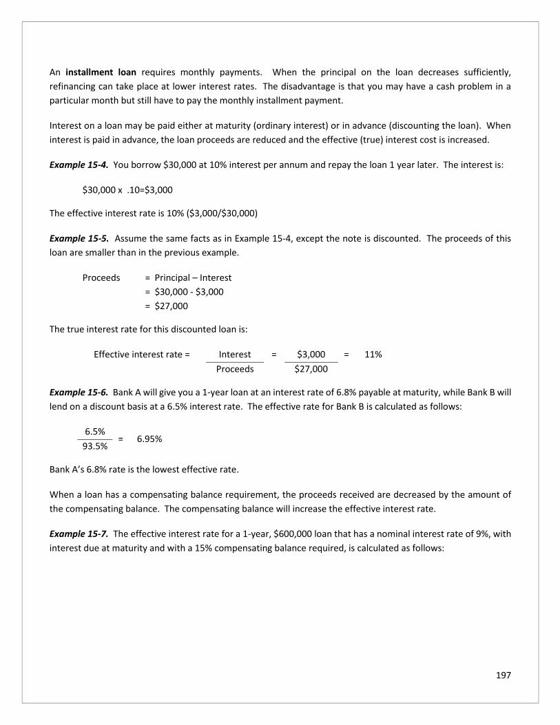
197

An installment loan requires monthly payments. When the principal on the loan decreases sufficiently,

refinancing can take place at lower interest rates. The disadvantage is that you may have a cash problem in a

particular month but still have to pay the monthly installment payment.

Interest on a loan may be paid either at maturity (ordinary interest) or in advance (discounting the loan). When

interest is paid in advance, the loan proceeds are reduced and the effective (true) interest cost is increased.

Example 15-4. You borrow $30,000 at 10% interest per annum and repay the loan 1 year later. The interest is:

$30,000 x .10=$3,000

The effective interest rate is 10% ($3,000/$30,000)

Example 15-5. Assume the same facts as in Example 15-4, except the note is discounted. The proceeds of this

loan are smaller than in the previous example.

Proceeds = Principal – Interest

= $30,000 - $3,000

= $27,000

The true interest rate for this discounted loan is:

Effective interest rate = Interest = $3,000 = 11%

Proceeds $27,000

Example 15-6. Bank A will give you a 1-year loan at an interest rate of 6.8% payable at maturity, while Bank B will

lend on a discount basis at a 6.5% interest rate. The effective rate for Bank B is calculated as follows:

6.5% = 6.95%

93.5%

Bank A’s 6.8% rate is the lowest effective rate.

When a loan has a compensating balance requirement, the proceeds received are decreased by the amount of

the compensating balance. The compensating balance will increase the effective interest rate.

Example 15-7. The effective interest rate for a 1-year, $600,000 loan that has a nominal interest rate of 9%, with

interest due at maturity and with a 15% compensating balance required, is calculated as follows:

198

Interest rate x principal =

.09 x $600,000

Percentage of proceeds available x Principal (1.00 - .15) x $600,000

= $54,000

$510,000

= 10.6%

Example 15-8. Assume the same facts as in Example 15-7, except that the loan is discounted. The effective

interest rate is:

Interest rate x principal

=

.09 x $600,000

Percentage of proceeds available x Principal less

compensating balance

(0.85 x $600,000) - $54,000

=

$54,000_____

$510,000 - $54,000

= 11.8%

Example 15-9. You have a credit line of $400,000, but you must maintain a compensating balance of 6% on

outstanding loans and a compensating balance of 5% on the unused credit. The interest rate on the loan is 6%.

You borrow $275,000. The required compensating balance is:

.06 x $275,000 = $16,500

.05 x 125,000 = 6,250

$22,750

The effective interest rate (with line of credit) is:

Interest rate (on loan) x Principal =

0.06 x $275,000

Principal - Compensating balance $275,000 - $22,750

=

$16,500

$252,250

= 6.5%

199

Commercial Paper

Commercial paper can be issued only if you possess a very high credit rating. Therefore, the interest rate is less

than that of a bank loan, typically 1 /2% below the prime interest rate. Commercial paper is unsecured and sold

at a discount (below face value). The maturity date is usually less than 270 days, otherwise, registration with the

Securities and Exchange Commission (SEC) is needed. When a note is sold at a discount, it means that interest is

immediately deducted from the face of the note by the creditor, but you will pay the full face value. Commercial

paper may be issued through a dealer or directly placed to an institutional investor. It ordinarily does not have an

active secondary market.

The benefits of commercial paper are that no security is required, the interest rate is typically less than through

bank or finance company borrowing, and the commercial paper dealer often offers financial advice. The

drawbacks are that commercial paper can be issued only by large, financially sound companies, and commercial

paper dealings relative to bank dealings are impersonal.

Example 15-10. You issue $500,000 of commercial paper every 2 months at a 13% rate. There is a $1 000

placement cost each time. The percentage cost of the commercial paper is:

Interest ($500,000 x .13) $65,000

Placement cost ($1,000 x 6) 6,000

Cost $71,000

Percentage cost of commercial paper $71,000

$500,000 = 14.2%

Receivable Financing

In accounts receivable financing, the accounts receivable are the security for the loan as well as the source of

repayment. Accounts receivable financing generally takes place under the following conditions:

• Receivables are a minimum of $25,000

• Sales are a minimum of $250,000.

• Individual receivables are at a minimum of $100.

• Receivables apply to selling merchandise rather than rendering services.

• Customers are financially strong.

• Sales returns are not great.

• Title to the goods passes to the buyer at shipment.

200

Receivable financing has several advantages, including avoiding the need for long-term financing and obtaining a

recurring cash flow. Accounts receivable financing has the drawback of high administrative costs when there are

many small accounts.

Accounts receivable may be financed under either a factoring or assignment (pledging) arrangement. Factoring

is the outright sale of accounts receivable to a bank or finance company without recourse. The purchaser of the

factoring arrangement (also called the factor) takes all credit and collection risks. The proceeds received are equal

to the face value of' the receivables less the commission charge, which is usually 2% to 4% higher than the prime

interest rate. The cost of the factoring arrangement is the factor's commission for credit investigation, interest

on the unpaid balance of advanced funds, and a discount from the face value of high-credit-risk receivables.

Remissions by customers are made directly to the factor.

The advantages of factoring are immediate availability of cash, reduction in overhead because the credit

examination function is no longer needed, obtaining of financial advice, receipt of advances as required on a

seasonal basis, and strengthening of the balance sheet position.

The disadvantages of factoring include both the high cost and the negative impression left with customers due to

the change in ownership of the receivables. Also, factors may antagonize customers by their demanding methods

of collecting delinquent accounts.

In an assignment (pledging), there is no transfer of the ownership of the accounts receivable. Receivables are

given to a finance company with recourse. The finance company usually advances between 50% and the face

value of the receivables in cash. You are responsible for charges, interest on the advance, and any resulting bad

debt losses. Remissions continue to be made directly to you.

The assignment of accounts receivable has the advantages of availability of cash, cash advances available on a

seasonal basis, and avoidance of negative customer feelings. The disadvantages include the high cost, the

continuance of the clerical function associated with accounts receivable, and the bearing of all credit risk.

You also must be aware of the impact of a change in account receivable policy on the cost of financing receivables.

When accounts receivable are financed, the cost of financing may rise or fall under different circumstances. For

example, when credit standards are relaxed, costs rise; when defaults are given to the finance company, costs

decrease; and when the minimum invoice amount of a credit sale is increased, costs decline. You should compute

the costs of accounts receivable financing and select the least expensive alternative.

Example 15-11. You have $120,000 per month in accounts receivable that a factor will purchase from you,

advancing you up to 80% of the receivables for an annual charge of 14% and a 1.5% fee on receivables purchased.

The cost of this factoring arrangement is:

Factor fee [.015 x ($120,000 x 12)] $21,600

Cost of borrowing [. 14 x ($1209000 x .8)] 13,440

Total cost $35,040

201

Example 15-12. Your factor charges a 3% fee per month. The factor lends you up to 75% of receivables purchased

for an additional 1% per month. Your credit sales are $400,000 per month. As a result of the factoring

arrangement, you save $6,500 per month in credit costs and a bad debt expense of 2% of credit sales.

XYZ Bank has offered an arrangement to lend you up to 75% of the receivables. The bank will charge 2% per

month interest plus a 4% processing charge on receivable lending.

The collection period is 30 days. If you borrow the maximum per month, should you stay with the factor or switch

to XYZ Bank? The cost of the factor is:

Purchased receivables .03 x $400,000) $12,000

Lending fee [.01 x (.75 x $400,000)] 3,000

Total cost $15,000

The cost of the bank financing is:

Interest [.02 x (.75 x $400,000)] $ 6,000

Processing charge [.04 x (.75 x $400,000)] 12,000

Additional cost of not using the factor:

Credit costs 6,500

Bad debts (.02 x $400,000) 8,000

Total cost $32,500

You should stay with the factor.

Inventory Financing

Inventory financing typically occurs when you have completely used your borrowing capacity on receivables. The

inventory itself must be good security for a loan, it must consist of marketable, nonperishable, and standardized

goods that have a quick turnover, and it should not be subject to rapid obsolescence. Inventory financing should

consider the price stability of the merchandise and the costs of selling it.

The advance is high when there is marketable inventory. In general, the financing of raw materials and finished

goods is about 75% of their value. The interest rate is approximately 3% to 5% over the prime interest rate. This

high-interest rate is one of the disadvantages of inventory financing. The restrictions placed on inventory

represent another drawback.

The types of inventory financing include a floating (blanket) lien, warehouse receipt, and trust receipt. They are

sources of secured financing. With a floating lien, the creditor's security lies in the aggregate inventory rather than

in its components. Even though you sell and restock, the lender's security interest continues. With a warehouse

receipt, the lender receives an interest in the inventory stored at a public warehouse; however, the fixed costs of

this arrangement are high. There may be a field warehouse arrangement in which the warehouse sets up a

202

secured area directly at your location. You have access to the goods but must continually account for them.

Generally, the inventory would not be in the immediate possession of the seller. With a trust receipt loan, the

creditor has title to the goods but releases them to you to sell on the creditor's behalf. As goods are sold, you

remit the funds to the lender. A good example of trust receipt use is in automobile dealer financing. The drawback

of the trust receipt arrangement is that a trust receipt must be given for specific items.

A collateral certificate may be issued by a third party to the lender guaranteeing the existence of pledged

inventory. The advantage of a collateral certificate is flexibility because merchandise does not have to be

segregated or possessed by the lender.

Example 15-13. You wish to finance $500,000 of inventory. Funds are required for 3 months. A warehouse

receipt loan may be taken at 16% with a 90% advance against the inventory's value. The warehousing cost is

$4,000 for the 3-month period. The cost of financing the inventory is:

Interest [. 16 x .90 x $500 000 x (3/12) $18,000

Warehousing cost $ 4,000

Total cost $22,000

Example 15-14. You show growth in operations but are presently experiencing liquidity difficulties. Six large

financially sound companies are responsible for 75% of your sales. Sales amount to $1,800,000, and net income

is $130,000. On the basis of the financial information that is provided in the following balance sheet, would you

be able to borrow on receivables or inventory?

Receivable financing can be expected since a high percentage of sales are made to only six large financially strong

companies. Receivables will thus show good collectability. It is also easier to control accounts.

Inventory financing is not likely, due to the high percentage of partially completed items. Lenders are reluctant

to finance inventory when a large work-in-process balance exists because the goods will be difficult to further

process and sell by lenders.

Assets

Current assets

Cash $27,000

Receivables 380,000

Inventory (consisting of 55% of work-in-progress) 320,000

Total current assets $727,000

Fixed Assets 250,000

Total Assets $977,000

Liabilities and Stockholders’ Equity

Current liabilities $260,000

Accounts payable 200,000

203

Loans payable 35,000

Total current liabilities $495,000

Non-current liabilities

Bond payable 110,000

Total liabilities $605,000

Stockholder’s equity

Common Stock $250,000

Retained earnings 122,000

Total stockholder’s equity 372,000

Total liabilities and stockholder’s equity $977,000

Inventory and receivables are not the only assets that may be used as security for short-term bank loans. Real

estate, plant and equipment, cash surrender value of life insurance policies, and securities may also be used. Also,

lenders are typically willing to advance a high percentage of the market value of bonds, and loans may also be

made based on a guaranty of a third party.


Banker’s Acceptances

A banker's acceptance is a draft, drawn by you and accepted by a bank, which orders payment to a third party at

a later date. The creditworthiness of the draft is of good quality because it has the backing of the bank, not the

client. It is, in essence, a debt instrument created out of a self-liquidating transaction. Bankers' acceptances are

often used to finance the shipment handling of both domestic and foreign merchandise. Acceptances act as short-

term financing because they typically have maturities of 180 days.

Example 15-15. A U.S. oil refiner arranges with its U.S. commercial bank for a letter of credit to a Saudi Arabian

exporter with whom the U.S has undertaken a transaction. The letter of credit regarding the shipment states that

the exporter can draw a time draft for a given amount on the U.S. bank. The exporter draws a draft on the bank

and negotiates it with a local Saudi Arabian bank, receiving immediate payment. The Saudi Arabian bank sends

the draft to the U.S, the latter accepts the draft, there is an acceptance to meet the maturity date.

Finance Company Loan

When credit is unavailable from a bank, you may have to go to a commercial finance company (e.g., CIT Financial).

The finance company loan has a higher interest rate than a bank, and generally it is secured. Typically, the amount

of collateral placed will be greater than the balance of the loan. Collateral includes accounts receivable,

204

inventories, and fixed assets. Commercial finance companies also finance the installment purchases of industrial

equipment by firms. A portion of their financing is sometimes obtained through commercial bank borrowing at

wholesale rates.

Conclusion

In short-term financing, the best financing tool should be used to meet your objectives. The financing instrument

depends upon your particular circumstances. Consideration is given to such factors as cost, risk, reactions, stability

of operations, and tax rate. Sources of short-term financing include trade credit, bank loans, bankers'

acceptances, finance company loans, commercial paper, receivable financing, and inventory financing. If you think

you will be short of cash during certain times, arrange for financing (e.g., a line of credit) in advance instead of

waiting for an emergency. If you are a small business, you would not have access to major capital markets. In fact,

the only options available, outside of owner financing, are bank loans and a line of credit from suppliers.

205


1. Which one of the following financial instruments generally provides the largest source of short-term credit for

small firms?

A. Installment loans

B. Commercial paper

C. Trade credit

D. Bankers' acceptances

2. If a firm borrows $500,000 at 10% and is required to maintain $50,000 as a minimum compensating balance at

the bank, what is the effective interest rate on the loan?

A. 10.0%

B. 11.1%

C. 9.1%

D. 12.2%

3. What is an example of secured short-term financing?

A. Commercial paper

B. A warehouse receipt

C. A revolving credit agreement

D. Line of credit

4. How would a small retail business most likely finance its merchandise inventory?

A. With commercial paper

B. With a warehouse receipt loan

C. With a line of credit

D. With a chattel mortgage

5. A manufacturing firm wants to obtain a short-term loan and has approached several lending institutions. All of

the potential lenders are offering the same nominal interest rate but the terms of the loans vary. Which of the

following combinations of loan terms will be most attractive for the borrowing firm?

A. Simple interest, no compensating balance

B. Discount interest, no compensating balance

C. Simple interest, 20% compensating balance required

D. Discount interest, 20% compensating balance required

206

Chapter 16: Intermediate-Term Financing

Learning Objectives


• Identify intermediate-term bank loans

• Recognize the advantages of revolving credit

This chapter considers intermediate-term loans, primarily from banks and leasing arrangements to meet your

financing needs. Intermediate-term loans include term loans, revolving credit, insurance company term loans,

and equipment financing.

Major Forms

Term Loans

Intermediate-term loans are typically loans with a maturity of more than 1 year but less than 5 years. They are

appropriate when short-term unsecured loans are not, such as when a business is acquired, new fixed assets are

purchased, and long-term debt is required. If you wish to float long-term debt or issue common stock but

conditions are unfavorable in the market, you may seek an intermediate loan to bridge the gap until long-term

financing can be undertaken on favorable terms.

The interest rate on an intermediate-term loan is typically higher than that on a short-term loan because of the

longer maturity period. The interest rate may be either fixed or variable (according to, for instance, changes in

the prime interest rate). The cost of an intermediate-term loan changes with the amount of the loan and your

financial strength.

Ordinary intermediate-term loans are payable in periodic, equal installments, except for the last payment, which

may be higher (referred to as balloon payment). The schedule of loan payments should be based on the cash flow

position to satisfy the debt. The periodic payment in a term loan is computed as follows:

207

Periodic payment = Amount of Loan

Present value factor

Example 16-1. You contract to repay a term loan in five equal year-end installments. The amount of the loan is

$150,000 and the interest rate is 10%. The payment each year is

$150,000 = $39,567.40

3.791

where 3.791 = T4 (10%, 5 years) = Present value of annuity for 5 years at 10% (from Table 11-4)

Example 16-2. You may want to determine the amount of loan, and what portion of the periodic payment

represents principal and interest. You take out a term loan to be paid off in 20 year-end annual installments of

$2,000 each. The interest rate is 12%. The amount of the loan is

$2,000 = Amount of Loan

7.469

Amount of Loan = $2,000 x 7.469 = $14,938.00

where 7.469 = T4(12%, 20 years) from Table 11-4

The amortization schedule for the first 2 years is shown in the table:

Year Payment Interesta Principal Balance

0 $14,938.00

1 $2,000 $1,792.56 $207.44 $14,730.56

2 $2,000 $1,767.67 $232.33 $14,498.23 a 12% times the balance of the loan at the beginning of the year.

When taking out an intermediate-term loan, you will encounter several kinds of restrictive provisions that are

designed to protect the lender. You may find that the agreement includes general provisions that are used in

most agreements and vary depending upon your situation. Examples are working capital and cash dividend

requirements. Or the agreement may contain routine (uniform) provisions that are employed in most agreements

and are applied universally. Examples are the payment of taxes and the maintenance of proper insurance to

ensure maximum lender protection. Lastly, you may encounter specific provisions that are tailored to a particular

situation. Examples are the placing of limits on future loans and the carrying of adequate life insurance for

executives.

The advantages of intermediate-term loans include the following:

• Intermediate-term loans provide flexibility in that the term may be altered as your financing requirements

change.

• Financial information is kept confidential since no public issuance is involved.

• The loan may be arranged quickly, relative to a public offering.

208

• These loans avoid the possible nonrenewal of a short-term loan.

• Public flotation costs are not involved.

The disadvantages of intermediate-term loans are as follows:

• Collateral and possible restrictive covenants are required, in contrast to commercial paper and unsecured

short-term bank loans.

• Budgets and financial statements may have to be submitted periodically to the lender.

• “Kickers”, or “Sweeteners”, such as stock warrants or a share of the profits, are sometimes requested by

the bank.

Revolving Credit

Revolving credit, usually used for seasonal financing, may have a 3-year maturity, but the notes evidencing

revolving credit are short, usually 90 days. The advantages of revolving credit are flexibility and ready availability.

Within the time period of the revolving credit, you may renew a loan or enter into additional financing up to a

maximum amount. There are typically fewer restrictions on revolving credit but at the cost of a slightly higher

interest rate.

Insurance Company Term Loans

Insurance companies and other institutional lenders may extend intermediate-term loans. Insurance companies

typically accept loan maturity dates exceeding 5 years, but their rate of interest is often higher than that of bank

loans. Insurance companies do not require compensating balances, but usually, there is a payment penalty, which

is typically not the case with a bank loan. You may take out an insurance company loan when you desire a longer

maturity range. Note: A compensating balance results in a higher effective borrowing cost because the

compensating balance is an amount of cash that the firm is unable to use. The cheapest terms, given that all

options have the same nominal interest rate, will be simple interest with no compensating balance.

Equipment Financing

Equipment may serve as collateral for a loan. An advance is made against the market value of the equipment.

The more marketable the equipment is, the higher the advance will be. Also considered is the cost of selling the

equipment. The repayment schedule is designed so that the market value of the equipment at any given time is

in excess of the unpaid loan principal.

Equipment financing may be obtained from banks, finance companies, and manufacturers of equipment.

Equipment loans may be secured by a chattel mortgage or a conditional sales contract. A chattel mortgage serves

as a lien on property excluding real estate. In a conditional sales contract, the seller keeps title to the equipment

until the buyer has satisfied the terms; otherwise, the seller will repossess the equipment. The buyer makes

periodic payments to the seller over a specified time period. A conditional sales contract is generally used if you

are a small company with a low credit rating.

209

The parties in a lease are the lessor who legally owns the property, and the lessee, who uses it in exchange for

making rental payments.

The following types of leases exist:

• Operating (service) lease. This type of lease includes both financing and maintenance services. You lease

property owned by the lessor. The lessor may be the manufacturer of the asset or it may be a leasing

company that buys assets from the manufacturer to lease to others. The lease payments under the

contract are typically not adequate to recover the full cost of the property. Maintenance and service are

provided by the lessor, and related costs are included in the lease payments. There usually exists a

cancellation clause, which provides you with the right to cancel the contract and return the property prior

to the expiration date of the agreement. The life of the contract is less than the economic life of the

property.

• Financial Lease. This type of lease does not typically provide for maintenance services, is non-cancelable,

and the rental payments equal the full price of the leased property. The life of the contract approximates

the life of the property.

• Sale and leaseback. With this lease arrangement, you sell an asset to another (usually a financial

institution) and then lease it back. This allows you to obtain cash from the sale and still have the property

for use.

• Leveraged lease. In a leveraged lease, a third party serves as the lender. Here, the lessor borrows money

from the lender to buy the asset. The property is then leased to you.

Leasing has several advantages, including the following:

• Immediate cash outlay is not required.

• Typically, a purchase option exists, allowing you to obtain the property at a bargain price at the expiration

of the lease. This provides the flexibility to make the purchase decision based on the value of the property

at the termination date.

• The lessor's expert service is made available.

• Typically, fewer financing restrictions (e.g., limitations on dividends) are placed by the lessor than are

imposed when obtaining a loan to purchase the asset.

• The obligation for future rental payment does not have to be reported on the balance sheet if the lease is

considered an operating lease.

• Leasing allows you, in effect, to depreciate land, which is not allowed if the land is purchased.

• In bankruptcy or reorganization, the maximum claim of lessors is 3 years of lease payments. With debt,

creditors have a claim for the total amount of the unpaid financing.

There are several drawbacks to leasing, including the following:

• In the long run, the cost is higher than if the asset is bought.

• The interest cost of leasing is typically higher than the interest cost on debt.

• If the property reverts to the lessor at the termination of the lease, you must either sign a new lease or

buy the property at higher current prices. Also, the salvage value of the property is realized by the lessor.

210

• You may have to retain property no longer needed (i.e., obsolete equipment).

• You cannot make improvements to the leased property without the permission of the lessor.

You may want to determine the periodic payment required on a lease.

Example 16-3. You enter into a lease for a $100,000 machine. You are to make 10 equal annual payments at

year-end. The interest rate on the lease is 14%. The periodic payment equals

$100,000 = $19,171

5.2161

where T4(10, 14%) = the present value of an ordinary annuity factor for n = 10, i = 14% = 5.2161 (Table 11-4).

Example 16-4. Use the same facts as those for Example 16-3, except that the annual payments are to be made at

the beginning of each year. The periodic payment is computed as follows:

Year Factor

0 1.0

1-9 4.946

5.946

$100,000 = $16,818

5.946

The interest rate associated with a lease agreement can also be computed. Divide the value of the leased property

by the annual payment to obtain the factor, which is then used to find the interest rate with the help of an annuity

table.

Example 16-5. You leased $300,000 of property and are to make equal annual payments at year-end of $40,000

for 11 years. The interest rate associated with the lease agreement is

$300,000 = 7.5

$40,000

Going to the present value of annuity table (T4) and looking across the 11-years entry to a factor nearest to 7.5,

we find 7.4987 at a 7% interest rate. Thus, the interest rate in the lease agreement is 7%.

The capitalized value of a lease can be found by dividing the annual lease payment by an appropriate present

value of annuity factor.

Example 16-6. Property is to be leased for 8 years at an annual rental payment of $140,000, payable at the

beginning of each year. The capitalization rate is 12%. The capitalized value of the lease is

211

Annual lease payment =

$140,000 = $25,163

Present value factor I + 4.5638

Often you must decide whether it is better to buy an asset or to lease it. Present value analysis may be used to

determine the cheapest alternative (see Chapter 12).

Conclusion

This chapter discussed intermediate-term loans, primarily from banks and leasing arrangements to meet your

financing needs. Intermediate-term loans include bank loans, revolving credit, insurance company term loans,

and equipment financing.

212


1. What is a major difference between operating and financial leases?

A. Operating leases usually do not provide for maintenance but financial leases do.

B. Operating lease contracts are written for a period that exceeds the economic life of the leased equipment.

C. Operating leases frequently contain a cancellation clause, whereas financial leases are not cancelable.

D. The lessee finances the assets leased for an operating lease.

213

Chapter 17: Long-Term Debt and Equity Financing

Learning Objectives


• Identify the process of investment banking

• Recognize issues for venture capital financing

• Recognize examples of types of long-term debt and their usefulness

• Identify examples of equity securities

This chapter will provide you with a deeper understanding of the financing of your company. You will learn the

fundamentals of long-term debt and equity financing. Equity financing consists of issuing preferred stock and

common stock. Long-term debt financing consists primarily of issuing bonds. Long-term financing is often used

to finance long-lived assets (e.g., land, plant) or construction projects.

First, the role of the investment banker is considered. Further, a comparison of public versus private placement

of securities is provided. The advantages and disadvantages of issuing long-term debt, preferred stock, and

common stock are presented as well. You will also learn what financing strategy is most appropriate, given a set

of circumstances, for your company.

Figure 17-1 shows the general picture with financing assets through debt and equity.

Figure 17-1. Financing Assets through Debt and Equity

214

The Role of Investment Bankers

Investment banking involves the sale of a security issue. Investment bankers conduct the following activities:

1. Underwriting. The investment banker buys a new security issue, pays the issuer, and markets the

securities. The underwriter's compensation is the difference between the price at which the securities

are sold to the public and the price paid to the issuing company.

2. Distributing. The investment banker markets your security issue.

3. Advising. The investment banker gives you advice regarding the optimal way to obtain funds. The

investment banker is knowledgeable about the alternative sources of long-term funds, debt and equity

markets, and the Securities and Exchange Commission (SEC) regulations.

4. Providing funds. The investment banker provides funds to you during the distribution period.

An issuer of new securities ordinarily selects an investment banker in a negotiated deal because of the costs

incurred in learning about the issuer and setting an issue price. The probability of closing a deal is high in a

negotiated deal, so the banker is willing to incur such costs. When several investment bankers form a group

because a particular issue is large and/or risky, they are termed a syndicate. A syndicate is a temporary association

of investment bankers brought together for the purpose of selling new securities. One investment banker among

the group will be selected to manage the syndicate (originating house) and to underwrite the major amount of

the issue. One bid price for the issue is made on behalf of the group, but the terms and features of the issue are

set by you.

The distribution channels for a new security issue appear in Figure 17-2.

Figure 17-2. Distribution Channels for a New Security Issue

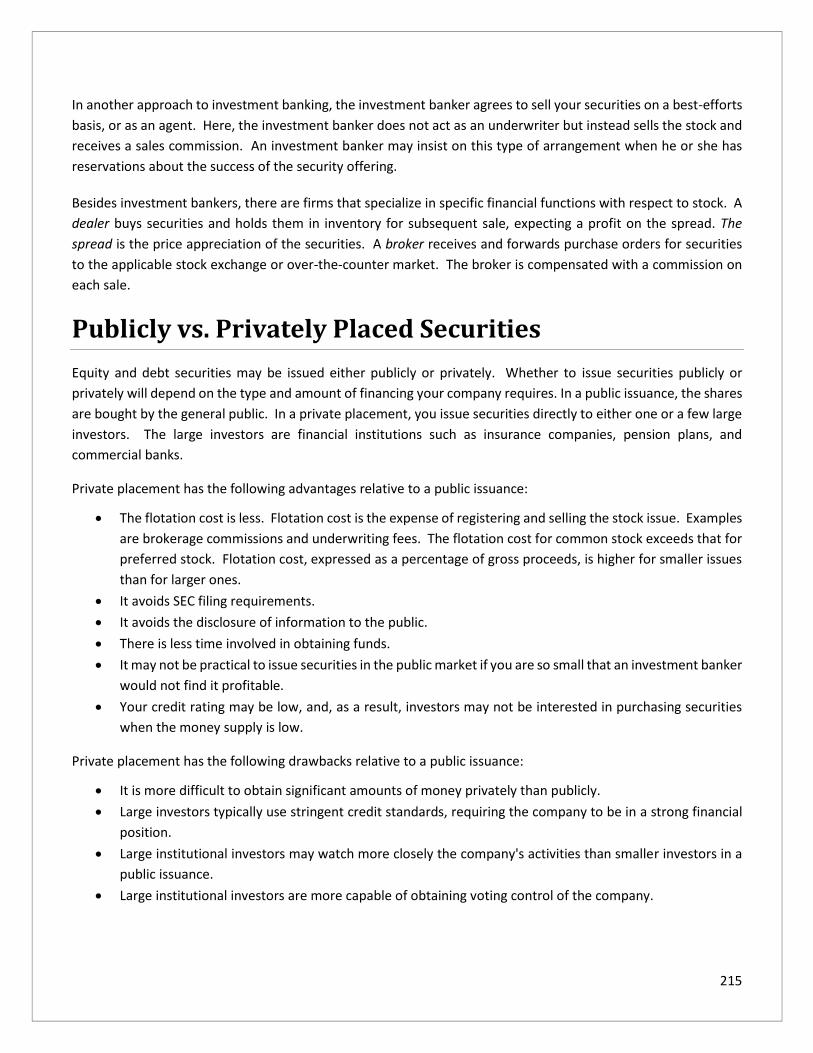
215

In another approach to investment banking, the investment banker agrees to sell your securities on a best-efforts

basis, or as an agent. Here, the investment banker does not act as an underwriter but instead sells the stock and

receives a sales commission. An investment banker may insist on this type of arrangement when he or she has

reservations about the success of the security offering.

Besides investment bankers, there are firms that specialize in specific financial functions with respect to stock. A

dealer buys securities and holds them in inventory for subsequent sale, expecting a profit on the spread. The

spread is the price appreciation of the securities. A broker receives and forwards purchase orders for securities

to the applicable stock exchange or over-the-counter market. The broker is compensated with a commission on

each sale.

Publicly vs. Privately Placed Securities

Equity and debt securities may be issued either publicly or privately. Whether to issue securities publicly or

privately will depend on the type and amount of financing your company requires. In a public issuance, the shares

are bought by the general public. In a private placement, you issue securities directly to either one or a few large

investors. The large investors are financial institutions such as insurance companies, pension plans, and

commercial banks.

Private placement has the following advantages relative to a public issuance:

• The flotation cost is less. Flotation cost is the expense of registering and selling the stock issue. Examples

are brokerage commissions and underwriting fees. The flotation cost for common stock exceeds that for

preferred stock. Flotation cost, expressed as a percentage of gross proceeds, is higher for smaller issues

than for larger ones.

• It avoids SEC filing requirements.

• It avoids the disclosure of information to the public.

• There is less time involved in obtaining funds.

• It may not be practical to issue securities in the public market if you are so small that an investment banker

would not find it profitable.

• Your credit rating may be low, and, as a result, investors may not be interested in purchasing securities

when the money supply is low.

Private placement has the following drawbacks relative to a public issuance:

• It is more difficult to obtain significant amounts of money privately than publicly.

• Large investors typically use stringent credit standards, requiring the company to be in a strong financial

position.

• Large institutional investors may watch more closely the company's activities than smaller investors in a

public issuance.

• Large institutional investors are more capable of obtaining voting control of the company.

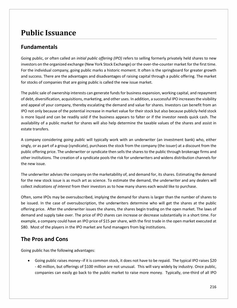
216

Public Issuance

Fundamentals

Going public, or often called an initial public offering (IPO) refers to selling formerly privately held shares to new

investors on the organized exchange (New York Stock Exchange) or the over-the-counter market for the first time.

For the individual company, going public marks a historic moment. It often is the springboard for greater growth

and success. There are the advantages and disadvantages of raising capital through a public offering. The market

for stocks of companies that are going public is called the new issue market.

The public sale of ownership interests can generate funds for business expansion, working capital, and repayment

of debt, diversification, acquisitions, marketing, and other uses. In addition, a successful IPO increases the visibility

and appeal of your company, thereby escalating the demand and value for shares. Investors can benefit from an

IPO not only because of the potential increase in market value for their stock but also because publicly-held stock

is more liquid and can be readily sold if the business appears to falter or if the investor needs quick cash. The

availability of a public market for shares will also help determine the taxable values of the shares and assist in

estate transfers.

A company considering going public will typically work with an underwriter (an investment bank) who, either

singly, or as part of a group (syndicate), purchases the stock from the company (the issuer) at a discount from the

public offering price. The underwriter or syndicate then sells the shares to the public through brokerage firms and

other institutions. The creation of a syndicate pools the risk for underwriters and widens distribution channels for

the new issue.

The underwriter advises the company on the marketability of, and demand for, its shares. Estimating the demand

for the new stock issue is as much art as science. To estimate the demand, the underwriter and any dealers will

collect indications of interest from their investors as to how many shares each would like to purchase.

Often, some IPOs may be oversubscribed, implying the demand for shares is larger than the number of shares to

be issued. In the case of oversubscription, the underwriters determine who will get the shares at the public

offering price. After the underwriter issues the shares, the shares begin trading on the open market. The laws of

demand and supply take over. The price of IPO shares can increase or decrease substantially in a short time. For

example, a company could have an IPO price of $15 per share, with the first trade in the open market executed at

$80. Most of the players in the IPO market are fund managers from big institutions.

The Pros and Cons

Going public has the following advantages:

• Going public raises money--if it is common stock, it does not have to be repaid. The typical IPO raises $20

- 40 million, but offerings of $100 million are not unusual. This will vary widely by industry. Once public,

companies can easily go back to the public market to raise more money. Typically, one-third of all IPO

217

issuers return to the public market within five years to issue a “seasoned equity offering.” Firms generally

prefer to obtain equity by retained earnings because of the flotation costs and market pressure involved

with the sale of new common stock. However, if a firm needs more money than can be generated from

retained earnings, a common stock offering may be necessary.

• As a company expands and becomes more valuable, its owners usually have most of their wealth tied up

in the company. By selling some of their stock in a public offering, they can reduce the riskiness of their

personal portfolios through this diversification of their holdings.

• Management often experiences an increase in prestige and reputation. Public firms have higher profiles

than private firms. This is important in industries where success requires suppliers and consumers to

make long-term investments. For example, software requires training and no manager wants to buy

software from a firm that may not be around for future improvements, upgrades, bug fixes, etc. The

suppliers’ and consumers’ perception of company success is a self-fulfilling prophecy. However, public

firms are usually bigger to begin with, and this may explain why public firms have a better image, on

average. Going public will not increase its sales. The important question is if going public improves the

company’s stockholders’ perception of success.

• Publicly traded stock can make a business more attractive to prospective and existing employees if stock

option and other stock compensation plans are offered. Employee stock-based programs are worth more

if transfer restrictions, such as those normally accompanying private company stock, are not placed on

the stock.

• Mergers and Acquisitions - Many private companies do not just appear on the “radar screen” of potential

acquirers. Being public makes it much easier for other firms to notice and analyze the company for

synergy.

• The use of proceeds from the sale of the issue is generally unrestricted.

• Public companies can acquire other businesses with stock, without depleting cash reserves.

• Other financing alternatives may improve.

Going public has the following disadvantages:

• Much jealously-guarded information must be disclosed. The guarded items include management salaries,

competitive position, transactions between the company and its management, and the identity of

significant customers and suppliers. In addition to the required disclosure of results of operations and

financial condition, public companies must be prepared to disclose information about the company,

officers, directors and certain shareholders. This information might include company sales and profits by

product line, salaries and other compensation of officers and directors, data about major customers,

competitive position, pending litigation, and related party transactions. By releasing the information it

will become available to competitors, customers, employees, and the general public. The information is

required in the initial registration statement and updated annually through annual reports, proxies and

other public disclosure documents. The company’s IPO filings are with the Securities and Exchange

Commission ( www.sec.gov).

• In addition to the time and effort required to prepare for the filing and offering, a company must be

prepared to incur the cost of going public. The principal costs include the underwriter's compensation,

legal and accounting fees, printing charges, and transfer agent and filing fees. A company expecting to go

http://www.sec.gov)/

218

public with a high-quality offering should anticipate spending $750,000 to $1 million, excluding

underwriter's commissions. The magnitude of these costs usually makes public offerings grossing less than

$50 million impractical. Furthermore, principals must remember that there is no guarantee that the

offering will be a success. With the exception of underwriter's compensation, the costs are incurred

regardless of the outcome. The cost of going public does not stop with the initial offering. Other costs

associated with being a public company are ongoing. Management must devote time and money to such

new areas as shareholder relations, public relations, public disclosures, periodic filings with the SEC, and

reviewing stock activity. All of this time and the time of the personnel hired to handle these functions

would be spent on other management tasks in a privately held company. There are other out-of-pocket

expenses. Shareholder meetings, annual and quarterly reports, public relations efforts and legal,

accounting and auditing fees must be paid. The total cost of these expenses vary from company to

company, but in most cases they range from $50,000 to $150,000 annually.

• Corporate decision making becomes more cumbersome as the company attempts to move from a

tightly-controlled, entrepreneurially-oriented company to a professionally managed one where

ownership and management are divorced. Any decision, long-term or short-term, may be manifested

promptly in the company's stock price. The company may worry constantly about improving quarterly

earnings (and stock prices) instead of trying to take a longer perspective in developing its strategy.

• All IPO participants in the coalition are jointly liable for each other’s actions. In practice, they were

routinely sued for various omissions in the IPO prospectus when the public market valuation fell below

the IPO offering price. The Private Securities Litigation Reform Act of 1995 protects the disclosure of firm

projections and forced the suing shareholders to have substantial participation in the firm. Although

nothing can eliminate lawsuits, this act reduces the likelihood of successful suits and therefore encourages

settlement terms.

• Since the number of shares outstanding increases when the company goes public, greater earnings must

be achieved to avoid reducing earnings per share.

• If the market price declines, many problems may result: management is usually personally blamed; the

flexibility of issuing stock to make acquisitions may be hampered; if the decline occurs soon after the

offering, litigation against everyone involved may take place; and other financing alternatives may

evaporate.

• If the company is sitting on a gold mine, future earnings have to be shared with outsiders. After a typical

IPO, about 40% of the company remains with insiders, but this can vary from 1% - 88%, with 20% - 60%

being the comfortable norm.

• Outsiders can take control and even fire the entrepreneur. There is pressure on the managers to produce

annual earnings gains, even when it may be in the shareholders’ best long-term interests to adopt a

strategy that reduces short term earnings but raises them in the future years. These factors have led a

number of newly public firms to go private in leveraged buyout deals where the managers borrow the

money to buy out the non-management stockholders. The use of IPOs is limited primarily because:

(a) there is a very high cost and much complexity in complying with federal and state laws governing

the sale of business securities; offering your business's ownership for public sale does little good

unless your company has sufficient investor awareness and appeal to make the IPO worthwhile;

and

219

(b) Management must be ready to handle the administrative and legal demands of widespread public

ownership. Of course, an IPO also means a dilution of the existing shareholders’ interests, and the

possibility of takeovers or adjustments in management control are present.

Here are some tips for avoiding the pitfalls of going public.

• Assemble the proper team. This involves selecting an underwriter, accountant, counsel, and perhaps some

new directors.

• When choosing an underwriter, distribution capacity is important.

• An underwriter appropriate for one company or one industry may be inappropriate for another. In

addition to technical ability, personalities and confidence should be considered.

• The selection of accountants and lawyers need careful examination.

• The registration process is complex, coupled with absolute liability for the company for material

misstatements or omissions--regardless of good faith or motive. It is important to remember that

malpractice insurance in the securities field is the most expensive of any specialty. That carries a message.

It is good to hire a "Big Five" or nationally prominent accounting firm because it enhances marketability

and confidence. The use of a large accounting and legal firm may be viewed by the underwriter as

insurance in the event of litigation.

• Securities laws are complicated. The sale of "securities" to the public is regulated by federal and state laws

that have two primary objectives:

(a) Require businesses to disclose material information about the company to investors, and

(b) Prohibit misrepresentation and fraud in the sale of securities. Under federal law, a "security" is

broadly defined and would include stocks, notes, bonds, evidence of indebtedness, and most

ownership interests. The law defines a "public offering" of a security not by the number of

investors to whom the stock is offered, but by the classification of whether the investors are

considered "sophisticated" or not. However, state law definitions of a "security" and of a "public

offering" can vary from the federal law.

Initial Public Offering Process

A company that is thinking of going public should start acting like a public company as much as two years in

advance. Several “to do’s” include developing a business plan and preparing detailed financial results on a regular

basis. Once a company decides to go public, it needs to choose its IPO team consisting of a lead investment bank,

accountant, lawyer, etc. The IPO process officially begins with an “all hands” meeting. This meeting usually takes

place six to eight weeks before a company officially registers with the SEC. At this meeting all members of the IPO

team assign certain duties to each individual and plan a timetable for going public.

The most important and time-consuming task facing the IPO team is the development of the prospectus, which is

a business document that basically serves as a brochure for the company. Since the SEC requires a “quiet period”

on firms once they file an IPO until 25 days after a stock starts trading, the prospectus will have to do most of the

talking and selling for the team. The prospectus includes all financial data for a company for the past five years.

It also includes information on the management team and a description of a company’s target market,

220

competitors, and growth strategy. There is much more information in the prospectus, and the underwriting team

goes to great efforts to make sure that it is all accurate.

The next step in the IPO process is the grueling worldwide tour, also known as the roadshow. The roadshow

usually lasts a week, with company management going to a new city every day to meet with prospective investors

and show off their business plan. The typical stops generally include the larger cities such as Los Angeles, San

Francisco, Boston, and Chicago. If necessary, international cities such as London and Hong Kong are included. The

management team’s performance on the roadshow is crucial. It helps determine the success of the IPO. The team

has to impress institutional investors and influence them to make significant long-term investments.

Once the roadshow ends and the final prospectus is distributed to investors, management officials meet with their

investment bank to decide on the final offering size and price. Investment banks generally suggest an appropriate

price based on expected demand for the deal and other market conditions. The pricing of an IPO is a delicate

balancing act. Investment firms have to be concerned with two different sets of customers, the company going

public, which wants to raise as much money as possible, and the investors buying the shares of stock, who expect

to see immediate gains from their investment. If public interest appears to be slowing it is common for the offering

price and number of shares to decrease from expected ranges. Sometimes, a company even has to postpone an

offering due to insufficient demand. If a deal is especially hot, the offering size and/or price can be raised from

initial projections.

Once the offering price has been agreed to, an IPO is declared effective. This is generally done after a market

closes, with the trading of the new stock beginning the next day. In the meantime, the chief underwriter works

to confirm its buy orders. The chief underwriter is responsible for ensuring smooth trading during the first crucial

days. This underwriter is legally allowed to support the price of a newly issued stock through buying shares in the

market or selling them short. They can also impose penalty bids on brokers to discourage “flipping’, which is when

investors sell shares of an IPO soon after the stock starts trading. An IPO is not declared final until seven days

after the firm’s initial market appearance. On rare occasions, an IPO can be canceled even after the stock begins

trading.

Alternatives to Going Public

Many businesses can sell stock to insiders or to a small group of investors without being subject to securities laws;

in effect, they can take advantage of alternatives to going public. However, it's not always clear where the

exemptions end, so you should always consult a knowledgeable attorney before selling any stock in your company.

The process of soliciting money from the public through the issuance and sale of securities requires a working

knowledge of the state and federal registration statements concerning the securities to be sold, complex

disclosure documents about the company with detailed information for potential investors, and financial

statements. Employing professionals (attorney, accountant, and sometimes a stock underwriter) to assist in the

process is a practical necessity.

While many small businesses sell interests in their companies that are "securities," as defined by federal or state

laws, the transactions are often exempt from registration regulations because the offerings are sufficiently small

in dollar amount, and they are restricted to a limited number and/or type of investor. These exempt offers of

221

securities are called "limited private offerings" and they can avoid much of the cost and delay of a public offering.

Unfortunately, to qualify for any of the exemptions, you must fit the criteria for both federal and state security

laws. Limited private offerings can be either debt or equity instruments, or a hybrid of both. For instance, a

convertible debt warrant would be a debt instrument that allowed the holder to convert the debt into an equity

interest at a certain time. These alternative offerings allow the business to tailor the amount of immediate equity

(ownership and control) that it relinquishes, and the amount of debt (cash outflow) that it can safely assume. In

this module, discussion of the use of limited private offerings is largely confined to equity financing.

Federal exemptions. At the federal level, the most popular exemption from registration requirements for small

businesses is Rule 504, commonly known as "Regulation D." Under this provision, private companies that are selling

less than $1 million worth of securities to any number of investors within a 12-month period are exempt from federal

registration requirements. Solicitations of investors by a private business may be made through almost any means,

including advertisements and seminars, and no specific disclosure requirements regarding the stock or the company

are required. Most startups and smaller businesses would fall within this exemption.

Even if a securities offering is exempt from the registration requirements of federal or state law, the anti-fraud

provisions of those laws may still apply. Therefore, you must take care to prevent misrepresentations or omissions in

the offering that create an overly optimistic picture of the investment. The investor should be provided with sufficient

information to make an informed decision regarding the investment.

Another exemption may be available to either private or publicly held companies that sell less than $5 million

within a 12-month period, if the sales are made only to "accredited investors" and no more than 35 such investors

are involved. Accredited investors include institutional investors (e.g., banks, brokers and dealers, insurance

companies), company insiders (e.g., officers and directors), and wealthy investors ("wealthy" meaning they have

more than $200,000 individual annual income or, individually or jointly with their spouse, have a net worth of

over $1 million).

A lesser degree of exemption from regulation exists for a private or publicly-held company that sells an unlimited

issuance of securities to an unlimited number of accredited investors, or to no more than 35 non-accredited but

"sophisticated investors" (sophisticated investors have sufficient knowledge and experience so that they

understand the risks of the sale, or the issuer reasonably believes the investors have these qualifications). Finally,

an exemption exists for private offerings of stock that are sold only to persons living in the same state where the

company is both incorporated and does significant business, although reliance upon this intra-state exemption is

subject to continual policing because the securities must remain within the state.

State exemptions. Because each state has regulations for securities, the local exemptions must be checked. Just

because a sale may be exempt from federal registration does not mean state registration is not required. State

securities laws are commonly referred to as "blue sky" laws because the regulations were originally enacted to

prevent unscrupulous issuers from selling “speculative schemes that have no more basis than so many feet of blue

sky." The state laws need not match the federal regulatory exemptions and even though a Uniform Securities Act

exists for states to follow, that Act has not been adopted by each state nor is it consistently interpreted in those

states which claim to follow it. The result is that consultation with a qualified professional is a practical necessity

before soliciting investors for sales of securities.

222

Venture Capital Financing

Venture capital firms supply funding from private sources for investing in select companies that have high, rapid

growth potential and a need for large amounts of capital. Venture capital firms speculate on certain high-risk

businesses producing a very high rate of return in a very short time. The firms typically invest for periods of three

to seven years and expect at least a 20 percent to 40 percent annual return on their investment.

When dealing with venture capital firms, keep in mind that they are under great pressure to identify and exploit

fast growth opportunities before more conventional financing alternatives become available to the target

companies. Venture capital firms have a reputation for negotiating tough financing terms and setting high

demands on target companies. Three bottom-line suggestions:

• Make sure to read the fine print.

• Watch for delay maneuvers (they may be waiting for your financial position to weaken further).

• Guard your trade secrets and other proprietary information zealously.

Venture capital financing may not be available, nor a good choice of financing, for many businesses. Usually,

venture capital firms favor existing businesses that have a minimal operating history of several years; financing of

startups is limited to situations where the high risk is tempered by special circumstances, such as a company with

extremely experienced management and a very marketable product or service. The target companies often have

revenues in excess of five million dollars and a preexisting capital investment of at least one million.

Venture capital firms research target companies and markets more vigorously than conventional lenders,

although the ultimate investment decision is often influenced by the market speculations of the particular venture

capitalists. Due to the amount of money that venture capital firms spend in examining and researching businesses

before they invest, they will usually want to invest at least a quarter of a million dollars to justify their costs.

Be wary of "shopping" innovative ideas to multiple venture capitalists or private investors. Use caution in revealing

any information you consider proprietary. Even if you already have intellectual property protection (e.g., a patent,

trademark, or copyright), you don't want to be forced to police your rights. Do your best to limit the details of

your particular innovation and seek confidentiality arrangements for additional protection of any preexisting legal

rights you may have.

The price of financing through venture capital firms is high. Ownership demands for an equity interest in 30

percent to 50 percent of the company are not uncommon even for established businesses, and a startup or higher

risk venture could easily require the transfer of a greater interest. Although the investing company will not

typically get involved in the ongoing management of the company, it will usually want at least one seat on the

target company's board of directors and involvement, for better or worse, in the major decisions affecting the

direction of the company.

223

The ownership interest of the venture capital firm is usually a straight equity interest or an ownership option in

the target company through either a convertible debt (where the debt holder has the option to convert the loan

instrument into stock of the borrower) or a debt with warrants to a straight equity investment (where the warrant

holder has the right to buy shares of common stock at a fixed price within a specified time period). An arrangement

that eventually calls for an initial public offering is also possible. Despite the high costs of financing through

venture capital companies, they offer tremendous potential for obtaining a very large amount of equity financing

and they usually provide qualified business advice in addition to capital.

Venture capital firms are located nationwide, and a directory is available through the National Venture Capital

Association, (www.nvca.org). In addition, other sources for venture capital can be found through bankers,

insurance companies, and business associations.

Sources of Long-Term Debt Financing

All companies incur debt; the amount of debt will largely depend on the company's available collateral. For long-

term debt financing, sources include mortgages and bonds. Either instrument may be appropriate, depending on

a company's circumstances. To determine which instrument will serve your company's needs best, you will need

to know the characteristics, advantages, and disadvantages of these long-term debt sources.

Mortgages

Mortgages are notes payable that have real assets as collateral and request periodic payments. Mortgages can

be issued to finance the purchase of assets, construction of a plant, and modernization of facilities. The bank

requires that the value of the property exceed its mortgage. Most mortgage loans are made for between 70% and

90% on the collateral. Mortgages may be obtained from a bank, a company, or another financial institution. It is

easier to obtain loans for multiple-use real assets than for single-use real assets.

There are two types of mortgages: a senior mortgage, which has first claim on assets and earnings, and a junior

mortgage, which has a subordinate lien.

A mortgage may have a closed-end provision that prevents you from issuing any additional debt of the same

priority against the same property. If the mortgage is open-ended, you can issue additional first-mortgage bonds

against the property.

Mortgages have a number of advantages, including favorable interest rates, fewer financing restrictions, an

extended maturity date for loan repayment, and relatively easy availability.

Bonds

Long-term debt principally takes the form of bonds payable and loans payable. A bond is a certificate indicating

that you have borrowed a given sum of money and agree to repay it. A written agreement, called an indenture,

224

describes the features of the bond issue (e.g., payment dates, call and conversion privileges (if any), and

restrictions). The indenture is a contract between your company, the bondholder, and the trustee. The trustee

makes sure that you meet the terms of the bond contract. In many instances, the trustee is the trust department

of a commercial bank. Although the trustee is an agent for the bondholder, it is selected by your company prior

to the issuance of the bonds. The indenture provides for certain restrictions on you such as a limitation on

dividends and minimum working capital requirements. If a provision of the indenture is violated, the bonds are

in default. The indenture may also have a negative pledge clause, which precludes the issuance of new debt taking

priority over existing debt in the event of liquidation. The clause can apply to assets currently held as well as to

assets that may be purchased in the future.

Computing Interest

Bonds usually come in $1,000 denominations. Many bonds have maturities of 10 to 30 years. The interest

payment to the bondholder is called nominal interest (coupon interest, stated interest), which is the interest on

the face value (maturity value, par) of the bond. Although the interest rate is stated on an annual basis, interest

on a bond is typically paid semiannually. Interest expense is tax-deductible.

Example 17-1. You issue a 10%, 10-year bond. The tax rate is 34%. The annual after-tax cost of the debt is 6.6%

(10% x 66%).

Example 17-2. You issue a $100,000, 8%, 10-year bond. The semiannual interest payment is $4,000 ($ 100,000 x

8% x 6/12). With a 34% tax rate, the after-tax semiannual interest is $2,640 ($4,000 x 66%).

A bond sold at face value is said to be sold at 100%. If a bond is sold below its face value (less than 100%) it is

issued at a discount. If a bond is sold above face value, (more than 100%) it is sold at a premium.

Why would your company's bond be sold at a discount or a premium? A bond may be sold at a discount when

the interest rate on the bond is below the prevailing market interest rate for that type of security. It may also be

issued at a discount if your company is risky, or there is a very long maturity period. A bond is issued at a premium

when the opposite market conditions exist.

Example 17-3. You issue a $100,000, 10%, 20-year bond at 94%. The maturity value of the bond is $100,000. The

annual cash interest payment is $10,000 (10% x $100,000). The proceeds received for the issuance of the bond

equal $94,000 ($100,000 x 94%). The amount of the discount is $6,000 ($100,000 - $94,000). The annual discount

amortization is $300 ($6,000/20).

The yield on a bond is the effective (real) interest rate you incur. The price of a bond depends on several factors

such as maturity date, interest rate, and collateral. Bond prices and market interest rates are inversely related.

For example, as market interest rates increase, the price of the existing bond falls because investors can invest in

new bonds paying higher interest rates.

Types of Bonds

The various types of bonds your company may issue are as follows:

225

1. Debentures. Because debentures are unsecured (no collateral) debt. Although no assets are mortgaged

as security for the bonds, debentures are secured by the full faith and credit of the issuing firm.

Debentures are a general obligation of the borrower and rank equally with convertible bonds. Only

companies with the best credit ratings can issue debentures because only the company's credit rating and

reputation secure the bonds

2. Subordinated debentures. The claims of the holders of these bonds are subordinated to those of senior

creditors. Debt with a prior claim over the subordinated debentures is set forth in the bond indenture.

Typically, in liquidation, subordinated debentures come after short-term debt.

3. Mortgage bonds. These are bonds secured by real assets. The first mortgage claim must be met before

a distribution is made to a second mortgage claim. There may be several mortgages for the same property

(e.g., building).

4. Collateral trust bonds. The collateral for these bonds is your company's security investments in other

companies (bonds or stocks), which are given to a trustee for safekeeping.

5. Convertible bonds. These may be converted to stock at a later date, based on a specified conversion ratio.

The conversion ratio equals the par value of the convertible security divided by the conversion price.

Convertible bonds are typically issued in the form of subordinated debentures. Convertible bonds are

more marketable and are typically issued at a lower interest rate than regular bonds because they offer

the conversion right to common stock. Of course, if bonds are converted to stock, debt repayment is not

involved. A convertible bond is a quasi-equity security because its market value is tied to the value of the

shares of stock into which the bond can be converted.

6. Income bonds. These bonds pay interest only if there is a profit. However, because it accumulates

regardless of earnings, the interest, if bypassed, must be paid in a later year when adequate earnings

exist.

7. Guaranteed bonds. These are debt issued by one party with payment guaranteed by another.

8. Serial bonds. A portion of these bonds comes due each year. At the time serial bonds are issued, a

schedule shows the yields, interest rates, and prices for each maturity. The interest rate on the shorter

maturities is lower than the interest rate on the longer maturities because less uncertainty exists

regarding the future.

9. Deep discount bonds. These bonds have very low-interest rates and thus are issued at substantial

discounts. The return to the holder comes primarily from appreciation in price rather than from interest

payments.

10. Zero-coupon bonds. These bonds do not provide for interest. The return to the holder is in the form of

appreciation in price.

226

11. Variable-rate bonds. The interest rates on the bonds are adjusted periodically to changes in money

market conditions. These bonds are popular when there is uncertainty about future interest rates and

inflation.

12. Junk bonds These bonds are high risk and therefore high-yield securities that are normally issued when

the debt ratio is very high. Thus, the bondholders have as much risk as the holders of equity securities.

Such bonds are not highly rated by credit evaluation companies. Junk bonds have become accepted

because of the tax-deductibility of the interest paid.

13. Inflation-linked bonds. These bonds have coupons (and the principal amount as well) that are adjusted

according to the rate of inflation. The U.S. Treasury Inflation Protection Securities (TIPS) is an example.

A summary of the characteristics and priority claims associated with bonds appears in Table 17-1.

Bond Ratings

Financial advisory services (e.g., Standard and Poor’s, Moody's) rate publicly traded bonds according to risk in

terms of the receipt of principal and interest. An inverse relationship exists between the quality of a bond issue

and its yield. That is, low-quality bonds will have a higher yield than high-quality bonds. Hence, a risk-return

trade-off exists for the bondholder. Bond ratings are important because they influence marketability and the cost

associated with the bond issue.

The Advantages and Disadvantages

You will need to determine whether or not your company should issue long-term debt.

The advantages of issuing long-term debt include the following:

• Interest is tax-deductible, while dividends are not.

• Bondholders do not participate in superior earnings of your firm.

• The debt is repaid in cheaper dollars during inflation.

• There is no dilution of company control.

• Financing flexibility can be achieved by including a call provision in the bond indenture. A call provision

allows your company to pay the debt before the expiration date of the bond.

• It may safeguard your company's future financial stability (e.g., in times of tight money markets when

short-term loans are not available.)

Table 17-1. Summary of Characteristics and Priority Claims of Bonds

Bond Type Characteristics Priority of Lender’s Claim

Debentures Available only to financially strong

companies. Convertible bonds are typically

debentures.

General creditor

227

Subordinated debentures Comes after senior debt holders General Creditor

Mortgage bonds Collateral is real property or buildings. Paid from the proceeds from the sale of

mortgaged assets. If any deficiency

exists, general creditor status applies.

Collateral trust bonds Secured by stock and(or) bonds owned by

the issuer. Collateral value is usually 30%

more than bond value.

Paid from the proceeds of stock and (or)

bond that is collateralized. If there is a

deficiency, general creditor, general

creditor, status applies.

Income bonds Interest is only paid if there is net income.

Often issued when a company is in

reorganization because of financial

problems.

General creditor.

Deep-discount (and zero-

coupon) bonds

Issued at very low or no (zero) coupon rates.

Issued at prices significantly below face

value. Usually callable at par value.

Unsecured or secured status may apply

depending on the features of the issue.

Variable-rate-bonds Coupon rate changes within limits based on

changes in money or capital market rates.

Appropriate when uncertainty exists

regarding inflation and future interest rates.

Because of the automatic adjustment to

changing market conditions, the bonds sell

near face value.

Unsecured or secured status may apply

depending on the features of the issue.

The following disadvantages may apply to issuing long-term debt:

• Interest charges must be met regardless of your company's earnings.

• Debt must be repaid at maturity.

• Higher debt implies greater financial risk, which may increase the cost of financing.

• Indenture provisions may place stringent restrictions on your company.

• Over-commitments may arise because of forecasting errors.

Should you buy a bond? To investors, bonds have the advantages of a fixed interest payment each year and of

greater safety than equity securities because bondholders have a priority claim in the event of corporate

bankruptcy. To investors, bonds have the disadvantages of not participating in incremental earnings and of no

voting rights.

How does issuing debt stack up against equity securities to your company? The advantages of issuing debt rather

than equity securities are as follows: interest is tax-deductible, whereas dividends are not; during inflation, the

payback will be in cheaper dollars; no dilution of voting control occurs; and flexibility in financing can be achieved

by including a call provision in the bond indenture. The disadvantages of debt incurrence relative to issuing equity

securities are that fixed interest charges and principal repayment must be met irrespective of your firm's cash

flow position, and stringent indenture restrictions often exist.

228

The proper mixture of long-term debt to equity depends on company organization, credit availability, and the

after-tax cost of financing. Where a high degree of debt already exists, you should take steps to minimize other

corporate risks.

When should long-term debt be issued? Debt financing is more appropriate at these times:

1. The interest rate on debt is less than the rate of return earned on the money borrowed. By using other

people’s money (OPM), the after-tax profit of the company will increase. Stockholders have made an

extra profit with no extra investment!

2. Stability in revenue and earnings exists so that the company will be able to meet interest and principal

payments in both good and bad years. However, cyclical factors should not scare a company away from

having any debt. The important thing is to accumulate no more interest and principal repayment

obligations than can reasonably be satisfied in bad times as well as good.

3. There is a satisfactory profit margin so that earnings exist to meet debt obligations.

4. There is a good liquidity and cash flow position.

5. The debt/equity ratio is low so that the company can handle additional obligations.

6. Stock prices are currently depressed so that it does not pay to issue common stock at the present time.

7. Control considerations are a primary factor so that if common stock was issued, greater control might fall

in the wrong hands.

8. Inflation is expected so that debt can be paid back in cheaper dollars.

9. Bond indenture restrictions are not burdensome.

Tip: If your company is experiencing financial difficulties, it may wish to refinance short-term debt on a long-term

basis (e.g., by extending the maturity dates of existing loans). This may alleviate current liquidity and cash flow

problems.

As the default risk of your company becomes higher, so will the interest rate to compensate for the greater risk.

Recommendation: When a high degree of debt (financial leverage) exists, try to reduce other risks (e.g., product

risk) so that total corporate risk is controlled.

Bond Refunding

Bonds may be refunded before maturity through either the issuance of a serial bond or the exercise of a call

privilege on a straight bond. The issuance of serial bonds allows you to refund the debt over the life of the issue.

A call feature in a bond enables you to retire it before the expiration date, The call feature is included in many

corporate bond issues.

When future interest rates are expected to drop, a call provision is recommended. Such a provision enables your

firm to buy back the higher interest bond and issue a lower-interest one. The timing for the refunding depends

on expected future interest rates. A call price is typically set in excess of the face value of the bond. The resulting

call premium equals the difference between the call price and the maturity value. Your company pays the

premium to the bondholder in order to acquire the outstanding bonds prior to the maturity date. The call

premium is usually equal to one year's interest if the bond is called in the first year, and it declines at a constant

229

rate each year thereafter. Also involved in selling a new issue are flotation costs (e.g., brokerage commissions,

printing costs).

A bond with a call provision typically will be issued at an interest rate higher than one without the call provision.

The investor prefers not to face a situation where your company can buy back the bond at its option prior to

maturity. The investor would obviously desire to hold onto a high-interest bond when prevailing interest rates

are low.

Example 17-4. A $100,000, 8% 10-year bond is issued at 94%. The call price is 103%. Three years after the issue,

the bond is called, The call premium is equal to

Call price $103,000

Less: Face value of bond (100,000)

Call premium $ 3,000

The desirability of refunding a bond requires present value analysis, which was discussed in Chapter 12.

Example 17-5. Your company has a $20 million, 10% bond issue outstanding that has 10 years to maturity. The

call premium is 7% of face value. New 10-year bonds in the amount of $20 million can be issued at an 8% interest

rate. Flotation costs of the new issue are $600,000.

Refunding of the original bond issue should occur as shown below.

Old interest payments ($20,000,000 x 0. 10) $2,000,000

Less: New interest payments ($20,000,000 x 0.08) (1,600,000)

Annual savings $ 400,000

Call premium ($20,000,000 x 0.07) $1,400,000

Flotation cost 600,000

Total cost $2,000,000

Year Calculation Present Value

0 -$2,000,000 x 1 -$2,000,000

1-10 $ 400,000 x 6.71a 2,684,000

Net present value $ 684,000

a 6.71 = T4 (8%, 10 years) from Table 11-4

Sinking fund requirements may exist in a bond issue. With a sinking fund, ' you put aside money to buy and retire

part of a bond issue each year. Usually, there is a mandatory fixed amount that must be retired, but occasionally

the retirement may relate to your company's sales or profit for the current year. If a sinking fund payment is not

made, the bond issue may be in default.

230

Equity Securities

We will now discuss equity financing consisting of preferred stock and common stock. The advantages and

disadvantages of issuing preferred and common stock are addressed, along with the various circumstances in

which one financing source is better suited than the other. Stock rights are also described.

Preferred Stock

Preferred stock is a hybrid between bonds and common stock. Preferred stock comes after debt but before

common stock in liquidation and in the distribution of earnings. Preferred stock may be issued when the cost of

common stock is high. It is best to issue preferred stock when your company has excessive debt and an issue of

common stock might result in control problems. Preferred stock is a more expensive way to raise capital than a

bond issue because the dividend payment is not tax-deductible.

Preferred stock may be cumulative or noncumulative. Cumulative preferred stock means that if any prior year's

dividend payments have been missed, they must be paid before dividends can be paid to common stockholders.

If preferred dividends are in arrears for a long time, your company may find it difficult to resume its dividend

payments to common stockholders. With noncumulative preferred stock, your company does not need to pay

missed preferred dividends. Preferred stock dividends are limited to the rate specified, which is based on the

total par value of the outstanding shares. Most preferred stock is cumulative.

Example 17-6. As of December 31, 20X3, your company had 6,000 shares of $15 par value, 14% cumulative

preferred stock outstanding. Dividends were not paid in 20X1-and 20X2. Assuming that your company was

profitable in 20X3, the amount of the dividend to be distributed is

Par value of stock = 6,000 shares x $15 = $90,000

Dividends in arrears ($90,000 x 14% x 2 years) $25,200

Current year dividend ($90,000 x 14%) 12,600

Total dividend $37,800

Participating preferred stock means that if declared dividends exceed the amount typically given to preferred

stockholders and common stockholders, the preferred and common stockholders will participate in the excess

dividends. Unless stated otherwise, the distribution of the excess dividends will be based on the relative total par

values. Nonparticipating preferred stock does not participate with common stock in excess dividends. Most

preferred stock is nonparticipating.

Preferred stock may be callable, which means that you can purchase it back at a subsequent date at a specified

call price. The call provision is advantageous when interest rates decline since your company has the option of

discontinuing payment of dividends at an excessive rate by buying back preferred stock issued when bond interest

rates were high. Unlike bonds, preferred stock rarely has a maturity date. However, if preferred stock has a

sinking fund associated with it, this, in effect, establishes a maturity date for repayment.

231

In bankruptcy, preferred stockholders are paid after creditors and before common stockholders. In such a case,

preferred stockholders receive the par value of their shares, dividends in arrears, and the current year's dividend.

Any asset balance then goes to the common stockholders.

The cost of preferred stock usually follows changes in interest rates. Hence, the cost of preferred stock will most

likely be low when interest rates are low. When the cost of common stock is high, preferred stock issuance may

be achieved at a lower cost.

The cost of preferred stock can be determined by dividing the dividend payment by the net proceeds received.

Example 17-7. You issued preferred stock of $2 million. The flotation cost is 11% of the gross proceeds. The

dividend rate is 14%. The effective cost of the preferred stock is

Dividend =

0. 14 x $2,000,000

Net proceeds $2,000,000 - (0. 11 x $2,000,000)

=

$280,000 = 15.7%

$1,780,000

To your company, a preferred stock issue has the following advantages:

• Preferred dividends do not have to be paid (important during financial distress), whereas interest on debt

must be paid.

• Preferred stockholders cannot force your company into bankruptcy.

• Preferred shareholders do not share in unusually high profits because common stockholders are the real

owners of the business.

• If your company is growth-oriented, it can generate better earnings for its original owners by issuing

preferred stock with a fixed dividend rate than by issuing common stock.

• Preferred stock issuance does not dilute the ownership interest of common stockholders in terms of

earnings participation and voting rights.

• Your company does not have to collateralize its assets as it may have to do if bonds are issued.

• The debt to equity ratio is improved.

To your company, preferred stock has the following disadvantages:

• Preferred stock requires a higher yield than bonds because of greater risk.

• Preferred dividends are not tax-deductible.

• There are higher flotation costs than with bonds.

The advantages of preferred stock over bonds are that one can omit a dividend readily, no maturity date exists,

and no sinking fund is required. Preferred stock also has a number of advantages over common stock. It avoids

dilution of control and the equal participation in profits that are afforded to common stockholders. The

disadvantages of preferred stock issuance compared to bonds are that it requires a higher yield than debt because

it is riskier to the holder. Also, dividends are not tax-deductible.

232

To an investor, preferred stock offers several advantages. First, preferred stock usually provides a fixed dividend

payment. Second, preferred stockholders' claims come before common stockholders' in the event of corporate

bankruptcy. Third, preferred dividends are subject to an 80% dividend exclusion for corporate investors. For

example, if a company holds preferred stock in another company and receives dividends of $10,000, only 20% (or

$2,000) is taxable. On the other hand, interest income on bonds is fully taxable. Unfortunately, the individual

investor does not qualify for the 80% dividend exclusion.

To an investor, preferred stock represents several disadvantages. For instance, the return is limited because of

the fixed dividend rate. Also, there is greater price fluctuation with preferred stock than with bonds because of

the lack of a maturity date. Lastly, preferred stockholders cannot require the company to pay dividends if the firm

has insufficient earnings.

Common Stock

We will now discuss everything you should know about common stock. The owners of a corporation are called

stockholders. They elect the board of directors, who in turn choose the company's officers. When the election

takes place, management sends proxy statements, which ask stockholders to give management the right to vote

their stock. Effective control of the corporation can exist with less than 50% common stock ownership since many

stockholders do not bother to vote. Stockholders have limited liability in that they are not personally liable for

the debts of the firm.

Common stock refers to the residual equity ownership in the business. Common stockholders have voting power,

but their claims come after preferred stockholders in receiving dividends and in liquidation. Common stock does

not involve fixed charges, maturity dates, or sinking fund requirements.

Authorized -shares are the maximum shares that can be issued according to the corporate charter. Issued shares

represent the number of authorized shares that have been sold by the company. Outstanding shares are the

issued shares held by the investing public. Treasury stock is stock that has been reacquired by the firm. It is not

retired but instead held for possible future resale, a stock option plan, use in purchasing another company, or the

prevention of a takeover by an outside group. Outstanding shares are thus equal to the issued shares less the

treasury shares. Dividends are based on outstanding shares.

The par value of a stock is a stated amount of value per share specified in the corporate charter.

If your company is closely held, it only has a few stockholders, who keep full control. There is no requirement to

publicly disclose corporate financial data. But a company with 500 or more stockholders must file an annual

financial statement with the Securities and Exchange Commission.

A company may issue different classes of common stock. Class A is stock issued to the public and typically has no

dividends. However, it usually has voting rights. Class B stock is typically kept by the company's organizers.

Dividends are usually not paid on it until the company has generated adequate earnings. Voting rights are

provided in order to maintain control.

233

The price of common stock moves in the opposite direction of market interest rates. For example, if market

interest rates increase, stock prices fall because investors will ' transfer funds out of stock into higher-yielding

money market instruments and bank accounts. Further, higher interest rates make it costly for a company to

borrow, resulting in lower profits and the subsequent decline in stock price.

Common stockholders have the following rights:

1. The right to receive dividends.

2. The right to receive assets upon the dissolution of the business.

3. The right to vote.

4. The preemptive right to buy new shares of common stock before their sale to the general public. In this

way, current stockholders can maintain their proportionate percentage ownership in the company.

5. The receipt of a stock certificate that evidences ownership. The stock certificate may then be sold by the

holder to another in the secondary security market.

1. The right to inspect the company's books.

A stockholder may make a significant profit if another firm wishes to take

the company over. The stockholder typically receives notice of the offer directly from his or her broker or by an

announcement in the financial pages of a newspaper (e.g., The Wall Street Journal.)

Disadvantages of common stock ownership are that common stockholders' claims come last in the event of

corporate bankruptcy and that dividends may be bypassed.

A number of options exist for equity financing in the case of small businesses, including the following:

1. Venture capital (investor) groups who invest in typically high-risk ventures.

2. Issuances directly to institutional investors (e.g., insurance companies, banks).

3. Issuances to relatives or friends.

4. Issuances to major customers and suppliers.

A determination of the number of shares that must be issued to raise adequate funds to satisfy a capital budget

may be needed.

Example 17-8. Your company currently has 650,000 shares of common stock outstanding. The capital budget for

the upcoming year is $1.8 million.

Assuming that new stock may be issued for $16 a share, the number of shares that must be issued to provide the

necessary funds to meet the capital budget is

Funds needed =

$1,800,000 = 112,500 shares

Market price per share $16

234

Example 17-9. Your company wants to raise $3 million in its first public issue of common stock. After its issuance,

the total market value of the stock is expected to be $7 million. Currently, there are 140,000 outstanding shares

that are closely held.

You want to compute the number of new shares that must be issued to raise the $3 million. The new shares will

have 3/7 ($3 million/$7 million) of the outstanding shares after the stock issuance. Thus, current stockholders

will be holding 4/7 of the shares.

140, 000 shares = 4/7 of the total shares

Total shares = 245, 000

New shares = 3/7 x 245, 000 = 105,000 shares

After the stock issuance, the expected price per share is

Price per share = Market value

= $7,000,000

= $28.57 Shares outstanding 245,000

When a company initially issues its common stock publicly, it is referred to as "going public." The estimated price

per share to sell the securities is equal to

Anticipated market value of the company Total outstanding shares

For an established company, the market price per share can be determined using Gordon's growth model (recall

from Chapter 12). The model is

Po = D1

r - g

or

Expected dividend

Cost of capital - Growth rate in dividends

Example 17-10. Your company expected the dividend for the year to be $10 a share. The cost of capital is 13%.

The growth rate in dividends is expected to be constant at 8%. The price per share is

Price per share = Expected dividend

Cost of capital - Growth rate in dividends

=

$10 =

$10 = $200

0.13 - 0.08 0.05

Another approach to pricing the share of stock for an existing company is through the use of the price/earnings

(P/E) ratio, which is equal to

235

Market price per share

Earnings per share

Example 17-11. Your company's earnings per share are $7. It is expected that the company's stock should sell at

eight times its earnings. The market price per share is therefore

P/E = Market price per share

Earnings per share

Market price per share = P/E multiple x Earnings per share

= 8 x $7 = $56

You may want to determine the market value of your company's stock. There are a number of different ways to

accomplish this.

Example 17-12. Assuming an indefinite stream of future dividends of $300,000 and a required return rate of 14%,

the market value of the stock equals

Market value = Expected dividends

= $300,000

= $2,142,857 Rate of return 0.14

If there are 200,000 shares, the market price per share is

Market value = $2, 142, 857

= $10.71 200,000

Example 17-13. Your company is considering a public issue of its securities. The average price/earnings multiple

in the industry is 15. The company's earnings are $400,000. There will be 100,000 shares outstanding after the

issuance of the stock. The expected price per share is

Total market value = Net income x Price/earnings multiple

= $400,000 x 15 = $6,000,000

Price per share = Market value

= $6,000,000

= $60 Shares 100,000

If your company has significant debt, it would be better off financing with an equity issue to lower overall financial

risk.

Financing with common stock has the following advantages: (1) there is no requirement to pay dividends; (2) there

is no repayment date; and (3) a common stock issue improves your company's credit rating relative to the issuance

of debt.

236

Financing with common stock has several disadvantages. For example, dividends are not tax-deductible. Also,

the ownership interest is diluted. The additional voting rights could vote to take control away from the current

ownership group. Further earnings and dividends are spread over more shares outstanding. Lastly, the flotation

costs of a common stock issue are more than with preferred stock and debt financing. It is always cheaper to

finance operations from internally generated funds because financing out of retained earnings involves no

flotation costs.

A summary comparison of bonds and common stocks is presented in Table 17-2.

Stockholders are typically better off when a company cuts back on dividends instead of issuing common stock as

a source of additional funds

Table 17-2. Summary Comparison of Bonds and Common Stock

Bonds Common Stock

• Bondholders are creditors • Stockholders are owners

• No voting rights exist. • Voting rights exist.

• There is a maturity date • There is no maturity date.

• Bondholders have prior claims on profits

and assets in bankruptcy.

• Stockholders have residual claims

• Interest payments represent fixed charges. • Dividend payments do not continue fixed

charges.

• Interest payments are deductible on the

tax return.

• There is no tax deductibility for dividend

payments

• The rate of return required by

bondholders is typically lower than that by

stockholders.

• The required rate of return by

stockholders is typically greater than that

by bondholders

When earnings are retained rather than new stock issued, the market price per share of existing stock will rise, as

indicated by higher earnings per share. Also, a company typically earns a higher rate of return than stockholders

so that by retaining funds the market price of the stock should appreciate. One caution, however: Lower dividend

payments may be looked at negatively in the market and may cause a reduction in the market price of stock due

to psychological factors.

Stock Rights

Stock rights are options to buy securities at a specified price at a later date. The preemptive right provides that

existing stockholders have the first option to buy additional shares. Exercising this right permits investors to

maintain voting control and protects against dilution in ownership and earnings.

237

Other Consideration

Debt or Equity Financing

Some companies obtain most of their funds from issuing stock and from earnings retained in the business. Other

companies borrow as much as possible and raise additional money from stockholders only when they can no

longer borrow. Most companies are somewhere in the middle. Companies use different mixes of financing,

depending on their circumstances.

In formulating a financing strategy in terms of source and amount, you should consider the following:

1. The cost and risk of alternative financing strategies.

2. The future trend in market conditions and how they will impact upon future fund availability and interest

rates. For example, if interest rates are expected to go up, you would be wise to finance with long-term

debt at the current lower interest rates.

3. The current debt to equity ratio. A very high ratio, for example, indicates financial risk, so additional funds

should come from equity sources.

4. The maturity dates of present debt instruments. For example, you should avoid making all debt come due

at the same time because in an economic downturn you may not have adequate funds to meet all the

debt.

5. The restriction in loan agreements. For instance, a restriction may exist placing a cap on the allowable

debt to equity ratio.

6. The type and amount of collateral required by long-term creditors.

7. The ability to change the financing strategy to adjust to changing economic conditions.

8. The amount, nature, and stability of internally generated funds. If stability exists in earnings generation,

the company is better able to meet debt obligations.

9. The adequacy of present lines of credit for current and future needs.

10. The inflation rate because, with debt, the repayment is in cheaper dollars.

11. The earning power and liquidity position of the firm. For example, a liquid company is better able to meet

debt payments.

12. The tax rate. For example, a higher tax rate makes debt more attractive because there are greater tax

savings from interest expense.

You have to select the best possible source of financing based on the fact

Example 17-14. Your company is considering issuing either debt or preferred stock to finance the purchase of a

plant costing $1.3 million. The interest rate on the debt is 6%. The dividend rate on the preferred stock is 3%.

The tax rate is 30%.

The annual interest payment on the debt is

6% x $1,300,000 = $78,000

238

The annual dividend on the preferred stock is

3% x $1,300,000 = $39,000

The required earnings before interest and taxes to meet the dividend payment is

$39,000 = $55,714

(1 - 0.30 )

If your company anticipates earning $55,714 without a problem, it should issue the preferred stock.

Example 17-15. Your company has sales of $30 million a year. It needs $6 million in financing for capital

expansion. The debt-to-equity ratio is 68%. Your company is in a risky industry, and net income is not stable. The

common stock is selling at a high P/E ratio compared to the competition. Under consideration is the issuance of

either common stock or a convertible bond.

Because your company is in a high-risk industry and has a high debt-to-equity ratio and unstable earnings, the

issuance of common stock is recommended.

Example 17-16. Your company is a mature one in its industry. There is limited ownership. The company has

vacillating sales and earnings. Your firm’s debt-to-equity ratio is 70% relative to the industry standard of 55%.

The after-tax rate of return is 16%. Since your company is a seasonal business, there are certain times during the

year when its liquidity position is inadequate. Your company is unsure about the best way to finance.

Preferred stock is one possible means of financing. Debt financing is not recommended because of the already

high debt to equity ratio, the fluctuation in profit, and the deficient liquidity posture. Because of the limited

ownership, common stock financing may not be appropriate because this would dilute the ownership.

Example 17-17. Your company wants to construct a plant that will take about 1 year to construct. The plant will

be used to produce a new product line, for which your company expects a high demand. The new plant will

materially increase corporate size. The following costs are expected:

Cost to build the plant $800,000

Funds needed for contingencies $100,000

Annual operating costs $175,000

The asset, debt, and equity positions of your company are similar to industry standards. The market price of the

company's stock is less than it should be, taking into account the future earnings of the new product line. What

would be the appropriate means to finance the construction?

Since the market price of the stock is less than it should be and considering the potential of the product line,

convertible bonds and installment bank loans might be appropriate means of financing because interest expense

is tax-deductible. Additionally, the issuance of convertible bonds might not require repayment, since the bonds

are likely to be converted to common stock because of the company's profitability. Installment bank loans can be

239

gradually paid off as the new product generates cash inflow. Funds needed for contingencies can be in the form

of open bank lines of credit.

If the market price of the stock was not at a depressed level, financing through equity would be an alternative

financing strategy.

Example 17-18. Your company wants to acquire another business but has not determined the optimal means to

refinance the acquisition. The current debt to equity position is within the industry guideline. In prior years,

financing has been achieved through the issuance of short-term debt.

Profit has shown vacillation and, as a result, the market price of the stock has fluctuated. Currently, however, the

market price of the stock is strong.

Your company's tax bracket is low.

The purchase should be financed through the issuance of equity securities for the following reasons:

1. The market price of the stock is currently at a high level.

2. The issuance of long-term debt will cause greater instability in earnings because of the high fixed interest

charges. Consequently, there will be more instability in the stock price.

3. The issuance of debt will result in a higher debt to equity ratio relative to the industry norm. This will

negatively impact the company's cost of capital and availability of financing.

4. Because it will take a long time to derive the funds needed for the purchase price, short-term debt should

not be issued. If short-term debt is issued, the debt would have to be paid before the receipt of the return

from the acquired business.

Resources

For borrowing money, lenders look for security in your assets and cash flow in addition to your character, so if you

can show a healthy balance sheet and a decent credit rating, you can borrow money easily on the Internet.

Many are web-based loan brokers representing a number of banks nationwide. You fill out an online application

detailing your business operation and your need for the loan, along with some personal information. Once the

website checks your personal and business credit ratings electronically, you can get an answer the same day for

loans under $50,000. Loans for larger amounts require additional documentation, usually submitted by mail, so

the approval process takes longer.

Websites also offer useful pages detailing the ins and outs of commercial finance, equipment leasing, government

funds, investment funds, real estate finance, venture capital, small business development councils and the Service

Corps of Retired Executives, a nonprofit organization of business mentors and counselors (www.score.org ).

In addition to these, lenders of every stripe maintain websites, including all of the big banks targeting business

customers, plus commercial finance companies and other sources of business loans. Most allow you to submit

online applications for business loans.

http://www.score.org/

240

It is not possible to do an equity deal by remote control on the Internet. However, the Internet can help you

simplify the first step in your search for equity or venture capital by getting your business plan in front of potential

investors. A number of good Web sites seek to help you make these connections, among them:

• The National Venture Capital Assn. (www.nvca.org), which lists over 300 venture capital and private equity

firms along with links to many of their Web sites, allowing you to gauge the firms' likes and dislikes.

• Garage.com (www.garage.com), which matches entrepreneurs and investors through a rigorous and

detailed "vetting" process probing business plans, management expertise, and the like.

Conclusion

Your company may finance long-term with debt or equity (preferred stock and common stock) funds. Each has

its own advantages and disadvantages. The facts of a situation have to be examined to determine which type is

best for your company's circumstances. A firm must select from among several methods of financing

arrangements when meeting its capital requirements. To acquire additional capital while attempting to maximize

earnings per share, a firm should normally select debt over equity initially, even though increased debt is

accompanied by interest costs and a degree of risk.

http://www.nvca.org/

http://www.garage.com/

241


1. How do preferred and common stock differ?

A. Failure to pay dividends on common stock will not force the firm into bankruptcy while failure to pay

dividends on preferred stock will force the firm into bankruptcy.

B. Common stock dividends are a fixed amount while preferred stock dividends are not.

C. Preferred stock has a higher priority than common stock with regard to earnings and assets in the event

of bankruptcy.

D. Preferred stock dividends are deductible as an expense for tax purposes while common stock dividends

are not.

2. Which one of the following statements correctly compares bond financing alternatives?

A. A bond with a call provision typically has a lower yield to maturity than a similar bond without a call

provision.

B. A convertible bond must be converted to common stock prior to its maturity.

C. A call provision is usually considered detrimental to the investor.

D. A sinking fund prohibits the firm from redeeming a bond issue prior to its final maturity.

3. What are debentures?

A. Income bonds that require interest payments only when earnings permit.

B. Subordinated debt and rank behind convertible bonds.

C. Bonds secured by the full faith and credit of the issuing firm.

D. Mortgage bonds secured by a lien on specific assets of the firm.

4. Zero-coupon bonds issued by corporations _________

A. Are initially sold at par value (a zero discount).

B. Are initially sold for a price above par value.

C. Are tax-free.

D. Require no cash outlay from the issuer until the bonds mature.

5. What are junk bonds?

A. Securities rated at less than investment grade

B. Worthless securities

C. Securities that are highly risky but offer only low yields

242

D. Related only to issues of "fallen angel" companies whose securities have been downgraded

6. The characteristics of venture capital include all of the following EXCEPT:

A. Initial private placement for the majority of issues.

B. A minimum holding period of 5 years for new securities.

C. The use of common stock for most placements.

D. A lack of liquidity for a period of time.

243

Chapter 18: Uses of Financial Statements

Learning Objectives


• Recognize the different financial statements and their uses

• Identify the major components of financial statements

A business entity is an economic unit that enters into business transactions that must be recorded, summarized,

and reported. Each business must have a separate set of accounting records and a separate set of financial

statements. The financial statements are the means of conveying to management and to interested outsiders a

concise picture of the value and profitability of the business for a given period of time.

The phrase generally accepted accounting principles (GAAP) is a set of standards and rules that are recognized as

a general guide to financial reporting. The primary objective of GAAP is to reduce the difference and

inconsistencies in accounting practice, thereby improving the comparability and credibility of financial reporting.

Public companies, nonprofit organizations, and government entities are required to prepare financial statements

in accordance with GAAP. An examination of what can be gained from these statements, and wherein the pitfalls

lie, is useful in setting up a program or strategy for planning and controlling profits.

The three main financial statements include the balance sheet, income statement, and statement of cash flows:

1. Balance sheet gives the company's position in terms of its assets, liabilities, and equity or net worth.

2. Income statement shows the company's sources of revenue, expenses, and net income.

3. Statement of cash flows reports the cash receipts, payments, and net change in cash on hand resulting

from the operating, investing, and financing activities of a company during a given period.

To make an informed judgment on the financial position and operating performance of the entity, managers should

have a good understanding of these statements, which are explained in this chapter.

244

Balance Sheet

The balance sheet or the statement of financial position portrays the financial position of an entity at a particular

point in time (as of a specific date), including an entity’s:

1. Assets (economic resources): What it owns , such as cash, land, and equipment;

2. Liabilities (economic obligations): How much it owes to vendors and lenders , such as loans payable and

mortgage payable; and

3. Owners' equity: Residual interest remaining after assets have been reduced by liabilities.

Each component is explained below.

Assets

Assets are economic resources that are owned by an organization and are expected to benefit future operations.

Assets may have definite physical forms such as buildings, machinery, or supplies. On the other hand, some assets

exist not in physical or tangible form, but in the form of valuable legal claims or rights, such as accounts receivables

from customers and notes receivables from debtors.

Assets that will be converted into cash within one year are classified as current. Examples are cash, marketable

securities, receivables, inventory, and prepaid expenses. Prepaid expenses include supplies on hand and advance

payments of expenses such as insurance and property taxes.

Assets having a life exceeding one year are classified as noncurrent. Examples are long-term investments, equipment,

and buildings. Equipment and buildings are often called plant assets or fixed assets.

Liabilities

Liabilities are debts owed to outsiders (creditors) and are frequently described on the balance sheet by titles that

include the word "payable." The liability arising from the purchase of goods or services on credit (on time) is called

accounts payable. The form of the liability when money is borrowed is usually a note payable, a formal written promise

to pay a certain amount of money, plus interest, at a definite future time. Accounts payable, as contrasted with a

note payable, does not involve the issuance of a formal promise written to the creditor, and it does not require

payment of interest. Other examples of liabilities include various accrued expenses.

Liabilities payable within one year are classified as current, such as accounts payable, notes payable, and taxes

payable. Obligations payable in a period longer than one year, for example, bonds payable, are termed long-term

liabilities.

Equity

Equity is a residual claim against the assets of the business after the total liabilities are deducted. Capital is the term

applied to the owner's equity in the business. Other commonly used terms for capital are owner's equity and net

245

worth. In a sole proprietorship, there is only one capital account since there is only one owner. In a partnership, a

capital account exists for each owner. In a corporation, capital represents the stockholders' equity, which equals the

capital stock issued plus the accumulated earnings of the business (called retained earnings). There are two types of

capital stock--common stock and preferred stock. Common stock entitles its owners to voting rights, while preferred

stock does not. Preferred stock entitles its owners to priority in the receipt of dividends and in repayment of capital

in the event of corporate dissolution.

Example 18-1. The equity of the owners of the business is quite similar to the equity commonly referred to with

respect to homeownership. If you were to buy a house for $150,000 by putting down 20 percent, i.e., $30,000 of your

own money and borrowing $120,000 from a bank, you would say that your equity in the $150,000 house was $30,000.

The balance sheet may be prepared either in report form or account form. In the report form, assets, liabilities, and

capital are listed vertically. In the account form, assets are listed on the left side and liabilities and capital on the right

side.

From the examples given, it is evident that there is a tie-in between the income statement and the balance sheet.

Biehl's net income of $5,800 (last item in her income statement from Example 18.1) is added to capital in her balance

sheet in the above example. In effect, the income statement serves as the bridge between two consecutive balance

sheets. Further, the net balance of the income statement accounts is used to adjust the Capital Account.

Figure 18-1 shows the relationship between the income statement and the balance sheet. In fact, the income

statement serves as a bridge between the two consecutive balance sheets.

FIGURE 18-1. BALANCE SHEET AND INCOME STATEMENT RELATIONSHIP

246

Example 18-2. (Report Form)

Joan Biehl

Balance Sheet

May 31, 20X1

ASSETS

Cash $10,000

Accounts Receivable 20,000

Office Supplies 10,500

Office Equipment 30,000

Total Assets $71,000

LIABILITIES AND CAPITAL

Liabilities

Accounts Payable $30,000

Capital

Balance, May 1, 20X1 $35,600

Net Income for May $5,800

Less withdrawals 400

Increase in Capital 5,400

Total Capital $41,000

Total Liabilities and Capital $71,000

Example 18-3. (Account Form)

Joan Biehl

Balance Sheet

May 31, 20X1

ASSETS LIABILITIES AND CAPITAL

Cash $10.000 Liabilities

Accounts Receivable 20,000 Accounts Payable $30,000

Office Supplies 10,500 Capital

Office Equipment 30,000 Balance, May 1, 20X1 $35,600

Net Income for May $5,800

Less: Withdrawals 400

Increase in Capital 5,400

Total Capital 41,000

Total Assets $71,000 Total Liabilities & Capital $71,000

247

Note: Simply put, with the balance sheet you are asking "how wealthy or poor is the company?," while with the income

statement you are asking "how did the company do last year?" and "did it make money and then how much." Neither

one is good enough to tell you about the financial health of the company. For example, the fact that the company

made a big profit does not necessarily mean it is wealthy, and vice versa. In order to get the total picture, you need

both statements to complement each other.

Unfortunately, you still have problems. You would like to know more about the company's financial shape (such as

the cash position of the company). However, neither the balance sheet nor the income statement provides

information about the flow of cash during the period. The statement of cash flows provides this information, which

will be discussed below.

Income Statement

The income statement measures operating performance for a specified time period (like for the year ended December

31, 20X1). The income statement shows the revenue, expenses, and net income (or loss) for a specified period. The

definition of each element is as follows.

Revenue

Revenue arises from the sale of merchandise (as by retail business), or the performance of services for a customer or

a client (as by a lawyer). Revenue from sales of merchandise or sales of services is often identified merely as sales.

Other terms used to identify sources of revenue include professional fees, commission revenue, and fares earned.

When revenue is earned it results in an increase in either Cash or Accounts Receivable.

Expenses

Expenses result from performing those functions necessary to generate revenue. The amount of an expense is either

equal to the cost of the goods sold, the value of the services received (e.g., salary expense), or the expenditures

necessary for conducting business operations (e.g. rent expense), during the period.

Net Income (Loss)

Net Income, also called profits or earnings, is the amount by which total revenue exceeds total expenses for the

reporting period. It should be noted that revenue does not necessarily mean receipt of cash and expense does not

automatically imply a cash payment. Note that net income and net cash flow (cash receipts less cash payments) are

different. For example, taking out a bank loan will generate cash, but this is not revenue since merchandise has not

been sold nor have services been provided. Further, capital has not been altered because of the loan.

248

Example 18-4. Joan Biehl is a self-employed consultant. For the month of May 20X1, she earned an income of $10,000

from services rendered. Her business expenses were: telephone $1,000, electricity $500, rent $2,000, secretarial

salary $300, and office supplies used, $400. Her income statement for the period is as follows:

Joan Biehl

INCOME STATEMENT

For the Month Ended May 31, 20X1

Revenue from professional services $10,000

Less: Operating Expenses

Telephone $1,000

Electricity 500

Rent 2,000

Secretarial Salary 300

Office Supplies 400

Total Operating Expenses 4,200

Net Income $ 5,800

Note that each revenue and expense item has its own account. This specifically enables one to better evaluate and

control revenue and expense sources and to examine relationships among account categories. For instance, the ratio

of telephone expenses to revenue is 10 percent ($1,000/$10,000). If in the previous month the relationship was 3

percent, Joan Biehl would, no doubt, attempt to determine the cause for this significant increase.

The balance sheet, also known as the statement of financial position, on the other hand, portrays the financial position

of the company at a particular point in time. It shows what is owed (assets), how much is owed (liabilities), and what

is left (assets minus liabilities, known as stockholders' equity or net worth). With the balance sheet, you cut the point,

freeze the action, and want to know about the company's financial position as of a certain date (like 12/31/20x1, the

end of the reporting year). It is a snapshot, while the income statement is a motion picture.

Statement of Cash Flows

Management and external interested parties have always recognized the need for a cash flow statement. Therefore,

in recognition of the fact that cash flow information is an integral part of both investment and credit decisions, the

Financial Accounting Standards Board (FASB) has issued ASC 230, Statement of Cash Flows. This pronouncement

requires that all business enterprises and not-for-profit organizations include a statement of cash flows as part of the

financial statements.

The statement of cash flows shows the sources and uses of cash, which is a basis for cash flow analysis for managers.

The statement aids you in answering vital questions like "where was money obtained?" and "where was money put

249

and for what purpose?" The following provides a list of more specific questions that can be answered by the

statement of cash flows and cash flow analysis:

1. Is the company growing or just maintaining its competitive position?

2. Will the company be able to meet its financial obligations?

3. Where did the company obtain funds?

4. What use was made of net income?

5. How much of the required capital has been generated internally?

6. How was the expansion in plant and equipment financed?

7. Is the business expanding faster than it can generate funds?

8. Is the company's dividend policy in balance with its operating policy?

9. Is the company's cash position sound and what effect will it have on the market price of stock?

Cash is vital to the operation of every business. How management utilizes the flow of cash can determine a firm's

success or failure. Financial managers must control their company's cash flow so that bills can be paid on time and

extra dollars can be put into the purchase of inventory and new equipment or invested to generate additional

earnings.

Operating Activities

Operating activities are connected to the manufacture and sale of goods or the rendering of services. They only

relate to income statement items. Cash inflows from operating activities include:

• Cash receipts from sales or servicing, such as from customers, licensees, and lessees.

• Interest and dividend receipts.

• Proceeds received from an insurance policy.

• Refunds from suppliers.

• Sale of trading securities.

• Award received from a lawsuit.

• Other operating receipts.

Cash outflows from operating activities include:

• Cash paid to buy materials and merchandise purchases.

• Cash paid for services.

• Payment of general and administrative expenses.

• Employee salary payments.

• Payments to suppliers.

• Insurance payments.

• Advertising and promotion payments.

• Payment for lawsuit damages.

• Cash refunds such as to customers for inferior goods.

• Interest payments.

250

• Income tax payments.

• Cash purchase of trading securities.

• Payment of duties, fines, and penalties.

• Charitable contribution payments.

• Other operating cash payments.

• Amortization of acquisition-date fair value adjustments under either the purchase or acquisition methods.

Under GAAP, most companies use the accrual basis of accounting. This method requires that revenue be recorded

when earned and that expenses be recorded when incurred. Revenue may include credit sales that have not yet

been collected in cash and expenses incurred that may not have been paid in cash. Thus, under the accrual basis

of accounting, net income will generally not indicate the net cash flow from operating activities. To arrive at net

cash flow from operating activities, it is necessary to report revenues and expenses on a cash basis. This is

accomplished by eliminating those transactions that did not result in a corresponding increase or decrease in cash

on hand.

Example 18-5. During 20x1, the Eastern Electric Supply Corporation earned $2,100,000 in credit sales, of which

$100,000 remained uncollected as of the end of the calendar year. Cash that was actually collected by the corporation

in 20x1 can be calculated as follows:

Credit sales $2,100,000

Less: Credit sales uncollected at year-end 100,000

Actual cash collected $2,000,000

A statement of cash flows focuses only on transactions involving the cash receipts and disbursements of a company.

As previously stated, the statement of cash flows classifies cash receipts and cash payments into operating, investing,

and financing activities.

Investing Activities

Investing activities include the results of the purchase or sale of debt and equity securities of other entities and

fixed assets. Cash inflows from investing activities include:

• Proceeds received from selling fixed assets.

• Selling available-for-sale or held-to-maturity securities in other companies.

• Collecting on loans made to debtors, principal portion.

• Insurance proceeds from property, plant and equipment damaged or destroyed.

Cash outlays for investing activities include:

• Acquiring fixed assets.

• Buying available-for-sale or held-to-maturity securities of other companies.

• Granting loans to borrowers.

• Cash purchases of businesses in a business combination.

251

Financing Activities

Financing activities include the issuance of stock and the reacquisition of previously issued shares (treasury stock),

as well as the payment of dividends to stockholders. Also included are debt financing and repayment. Cash inflows

from financing activities include:

• Funds received from issuing the company's own short-term or long-term debt (e.g., bonds payable, notes

payable, or mortgages payable).

• Funds received from selling the company's own equity securities. (Note: This also includes the subsequent

re-issuance of treasury stock.)

Cash outflows for financing activities include:

• Purchase of treasury stock.

• Cash dividend payments. (Note: Dividends declared but unpaid and stock dividends are noncash

transactions and are presented in a supplementary schedule titled “Noncash Investing and Financing

Activities.”)

• Retiring or paying off the principal on short-term or long-term debt. (This includes payments of principal

on capital lease obligations.)

• Other principal payments to long-term creditors.

• Payment of debt issue costs.

• Subsidiary dividends paid to noncontrolling interest shareholders.

Example 18-6. The following information pertains to Liverpool Sugar Corporation during 20x1.

1. The company had $1,004,000 in cash receipts from the sale of goods. Cash payments to acquire materials

for the manufacture of goods totaled $469,000, its payments on accounts and notes payable amounted

to $12,000, and it paid $136,000 in federal and state taxes.

2. The company sold all of its stock investment in Redondo Food Corporation, an unrelated entity, for

$100,000. It then bought a new plant and equipment for $676,000.

3. In 20x1, the company sold $300,000 of its 10%, ten-year bonds. It also issued another $50,000,000 in

preferred stock in return for land and buildings. The company paid a cash dividend of $36,000.

4. The company had a $198,000 cash balance at the beginning of the year.

The statement cash flows for the company would be presented as follows:

252

Liverpool Sugar Corporation

Statement of Cash Flows

for the Year Ended December 31, 20X1

Cash flows from operating activities:

Cash received from customers $1,004,000

Cash payment for acquisition of materials (469,000)

Cash payment for interest (12,000)

Cash payment for taxes (136,000)

Net cash provided by operating activities $ 387,000

Cash flows from investing activities:

Cash paid to purchase plant and equipment $(676,000)

Sale of long-term investment 1,000

Net cash used in investing activities (675,000)

Cash flows from financing activities:

Cash received from sale of bonds $ 300,000

Cash paid for dividends (36,000)

Net cash used in financing activities 264,000

Net decrease in cash and cash equivalents ( 24,000)

Cash and cash equivalents at the beginning of the year. 98,000

Cash and cash equivalents at the end of the year $ 74,000

Note that the issuance of the preferred stock in exchange for the land and buildings is a noncash transaction that

would be disclosed in a supplementary form at the end of the statement of cash flows.

253


The FASB issued ASU 2016-15, Statement of Cash Flows (Topic 230): Classification of Certain Cash Receipts and

Cash Payments, to create consistency and reduce diversity in practice in following cash flow items:

Cash Flow Item Cash Flow

Classification ASU 2016-15

Debt Prepayment or Debt Extinguishment

Costs Financing

Cash payments for debt prepayment or debt extinguishment costs should be classified as cash outflows for financing activities.

Settlement of Zero- Coupon Debt Instruments

Operating

Cash payments for the settlement of zero-coupon debt instruments, including other debt instruments with coupon interest rates that are insignificant in relation to the effective interest rate of the borrowing, should be classified as cash outflows for operating activities for the portion attributable to interest.

Financing Cash payment attributable to the principal should be classified as cash outflows for financing activities.

Payment of Contingent

Consideration Made After a Business

Combination

Investing Cash payments made soon after an acquisition’s consummation date (i.e., approximately three months or less) should be classified as cash outflows for investing activities.

Financing Cash payments made thereafter should be classified as cash outflows for financing activities up to the amount of the original contingent consideration liability.

Operating Cash payments made in excess of the amount of the original contingent consideration liability should be classified as cash outflows for operating activities.

Settlement of Insurance Claims

Classify based on the nature

of the loss

Cash payments received from the settlement of insurance claims should be classified on the basis of the nature of the loss.

Settlement of COLI & BOLI Policies

Investing Cash payments received from the settlement of corporate-owned life insurance (COLI) and bank-owned life insurance (BOLI) policies should be classified as cash inflows from investing activities.

Operating, Investing, or a

mix of both

Cash payments for premiums on COLI and BOLI policies may be classified as cash outflows for investing, operating, or a combination of investing and operating activities.

Distributions from Equity Method

Investees: Cumulative Earnings

Approach

Operating Distributions received up to the amount of cumulative equity earnings would be considered a return on investment and classified in operating activities.

Investing

Distributions as returns of investment (excess of cumulative distributions, excluding prior distributions determined to be returns of investment, over cumulative equity in earnings) are classified in investing activities.

Distributions from Equity Method

Operating Distributions as returns on investment (based on the nature of activity that generated the distributions) are classified in operating activities.

254

Investees: Nature of Distribution

Approach Investing

Distributions as returns of investment (based on the nature of activity that generated the distributions) are classified in investing activities.

Beneficial Interests in Securitization Transactions

Disclosed as Noncash

A transferor’s beneficial interest obtained in a securitization of financial assets is disclosed as a noncash activity.

Investing Cash receipts from a transferor’s beneficial interests in securitized trade receivable is classified in investing activities.

Cash Receipts & Payments More Than

One Class of Cash Flows

Based on its Nature

When each source or use of cash is separately identifiable, entities should classify each based on its nature.

Application of the

Predominance Principle

When each source or use of cash is not separately identifiable, entities should classify each based on its nature.

Conclusion

The traditional accounting statements--balance sheet, income statement and the required statement of cash flows--

have been and will continue to be the most important tools for both management and outsiders for use in gauging

the financial condition of a business. As a later chapter will show, additional insights into the performance of the

business can be gained by using financial ratio analysis.

255


1. The basic financial statements include a balance sheet, income statement, and statement of activities. True or

False?

2. What is the primary purpose of the balance sheet?

A. To reflect the fair value of the firm’s assets at some moment in time

B. To reflect the status of the firm’s assets in case of forced liquidation of the firm

C. To reflect assets, liabilities, and equity

D. To reflect the firm’s potential for growth in stock values in the stock market

3. A financial statement includes all of the following items: operating activities, financial activities, and investing

activities. What financial statement is this?

A. Statement of cash flows

B. Balance sheet

C. Income statement.

D. Statement of retained earnings

256

Chapter 19: Accounting Conventions and Recording

Financial Data

Learning Objectives


• Recognize the double-entry system and the accounting equation

• Recognize how to apply transaction analysis to simple business transactions in terms of the accounting

model

• Identify the entries entered into the journal

• Recognize how certain transactions affect the balance sheet

Financial decisions are usually formulated on the basis of information generated by the accounting system of the firm.

Proper interpretation of the data requires an understanding of the concepts and rules underlying such systems, the

convention adopted in recording information, and the limitation inherent in the information presented.

The transactions of most businesses are numerous and complex, affecting many different items appearing on the

financial statements. Therefore, a formal system of classification and recording is required for timely financial

reporting and managerial needs.

The aim of this chapter is to introduce the formal classification system of financial information commonly called

double-entry accounting. By acquiring background information about this system, you will be able to more clearly

understand the basic structure of the financial statements that were discussed in the previous chapter.

The Accounting Equation

Double-entry accounting is a system in which each business transaction affects and is recorded in two or more

accounts with equal debits and credits. An entity's financial position is reflected by the relationship between its assets

257

and its liabilities and equity. The accounting equation reflects these elements by expressing the equality of assets to

creditors' claims and owners' equity as follows:

ASSETS (A) = LIABILITIES (L) + EQUITY (E)

The equation in effect says that a company's assets are subject to the rights of debt holders and owners.

The accounting equation is the basis for double-entry accounting, which means that each transaction has a dual effect.

A transaction affects either both sides of the equation by the same amount or one side of the equation only, by

increasing and decreasing it by identical amounts and thus netting zero.

Example 19-1. Foster Architectural Company has assets of $700,000, and obligations of $300,000, and owner's equity

of $400,000. The accounting equation is

ASSETS = LIABILITIES + EQUITY

$700,000 = $300,000 + $400,000

If at the end of the reporting period, the firm derived a net income of $80,000, the accounting equation becomes


$780,000 = $300,000 + $480,000

If $60,000 was then used to pay creditors, the accounting equation becomes


$720,000 = $240,000 + $480,000

In the next example, we will illustrate how the transactions of a business are recorded and what effect they have on

the accounting equation.

Example 19-2. Lloyd Thomas, a consultant, experienced the following events in the month of January 20X1:

1. Started his consulting practice with a cash investment of $10,000 and office equipment worth $5,000

2. Purchased office supplies of $800 by paying cash

3. Bought a laptop computer for $500 on account from Office Depot

4. Paid $400 in salary to his staff

5. Received an electric bill for $300

6. Earned professional fees of $20,000, of which $12,000 was owed

7. Paid $300 to Office Depot

8. Withdrew $100 from the firm for personal use

9. Received $1,000 from one of the clients who owed him money

The transactions will now be analyzed.

258

Transaction 1. Thomas started his engineer consulting practice by investing $10,000 in cash and $5,000 in office

equipment. The assets Cash and Office Equipment are increased, and the equity is also increased for the total

investment of the owner.

Asset = Liabilities + Equity

Cash Office

Equipment (OE)

L. Thomas

Equity (E)

$10,000 $5,000 $15,000

Transaction 2. Acquired office supplies for cash, $800.

The asset Office Supplies goes up by $800 with a corresponding reduction in the asset Cash. This is an example of one

asset being used to acquire another one.

Assets = Liabilities + Equity

Cash (OE)

Office

Supplies (OS)

$10,000 $5,000 $15,000

___-800 ______ +800 _______

$9,000 $5,000 $800 $15,000

Transaction 3. Purchased a laptop computer on account, $500.

An asset, Office Equipment, is being acquired on credit, thereby creating a liability for future payment called Accounts

Payable. Accounts Payable is defined as the amount owed to suppliers.


Cash OE OS Accounts Payable (AP)

$9,200 $5,000 $800 $15,000

______ __+500 ____ +$500 _______

$9,200 $5,500 $800 $500 $15,000

Transaction 4. Paid salary, $400.

Cash and equity are both being reduced because of the wage expense. Equity is reduced because expenses of the

business decrease the equity of the owner.


Cash OE OS AP

$9,200 $5,500 $800 $500 $15,000

__-400 ______ ____ ____ ___-400

$8,800 $5,500 $800 $500 $14,600

Transaction 5. Received an electric bill for $300 (not paid). Liabilities are increased by $300 since the firm owes the

utility money for electricity supplied. Equity is reduced for the expense.

259


Cash OE OS AP

$8,800 $5,500 $800 500 $14,600

______ ______ ____ +300 ___-300

$8,800 $5,000 $800 $500 $14,300

Transaction 6. Earned fees of $20,000, of which $12,000 was received in cash and $8,000 was owed by clients.

Cash goes up by $12,000 and the Accounts Receivable (amounts owed to the business from customers) is created.

Professional fees earned are revenue to the business and hence increases the owner's equity. Thus, equity is increased

by $20,000.


Cash OE OS AR AP

$8,800 $5,500 $800 $800 $14,300

+12,000 ______ ____ +$8,000 ____ +20,000

$20,800 $5,500 $800 $8,000 $800 $34,300

Transaction 7. Paid $300 to Office Depot (in partial payment of the amount owed to them).

The payment lowers the asset Cash and reduces the liability Accounts Payable.


Cash OE OS AR AP

$20,800 $5,500 $800 $8,000 $800 $34,300

___-300 ______ ____ ______ _-300 _______

$20,500 $5,500 $800 $8,000 $500 $34,300

Transaction 8. Withdrew $100 for personal use.

Cash is reduced and so is equity. The personal withdrawal is, in effect, a disinvestment in the business and hence

reduces equity. It is not an expense in running the business.


Cash OE OS AR AP

$20,800 $5,500 $800 $8,000 $500 $34,300

___-100 ______ ____ ______ ____ ___-100

$20,400 $5,500 $800 $8,000 $500 $34,200

260

Transaction 9. Received $1,000 from clients who owed him money.

This increases Cash and reduces Accounts Receivable since the client now owes the business less money. One

asset is being substituted for another one.


Cash OE OS AR AP

$20,400 $5,500 $800 $8,000 $500 $34,300

_+1000 ______ ____ -1,000 ____ ___-100

$21,400 $5,500 $800 $7,000 $500 $34,200

Transaction 10. Worth (determined by an inventory count) of office supplies on hand at month's end, $600.

Since the worth of office supplies originally acquired was $800 and $600 is left on hand, the business used $200 in

supplies. This reduces the asset Office Supplies and correspondingly reduces equity. The supplies used up represent

office supplies expense.


Cash OE OS AR AP

$21,400 $5,500 $800 $7,000 $500 $34,200

______ ______ -200 ______ ____ ___-200

$21,400 $5,500 $800 $7,000 $500 $34,000

SUMMARY OF TRANSACTIONS

January 20X1


Cash OE OS AR AP

$10,000 $5,000 $15,000

___-800 _____ +800 ______

9,200 5,000 800 15,000

______ _+500 ____ +$500 ______

9,200 5,500 800 500 15,000

__-400 _____ ____ ___ __-400 Wage Expense

8,800 5,500 800 500 14,600

______ _____ ____ +300 __-300 Utility Expense.

8,800 5,500 800 800 14,300

+12,000 _____ ____ $8,000 ___ +20,000 Prof. Fee Revenue

20,800 5,500 800 8,000 800 34,300

__-300 _____ ____ _____ -300 _____

20,500 5,500 800 8,000 500 34,300

__-100 _____ ____ _____ ___ __-100 Drawing

20,400 5,500 800 8,000 500 34,200

261

+1,000 _____ ____ -1,000 ___ _____

21,400 5,500 7,000 500 34,200

_____ _____ -200 _____ ___ __-200 Off. Supplies Exp.

21,400 5,500 $600 $7,000 = 500 34,000

$34,500 = $34,500

The Account, Ledger, and Chart of Accounts

To prepare an equation Assets = Liabilities + Stockholders' Equity for each transaction would be extremely time-

consuming. Further, information about a specific item (e.g., accounts receivable) would be lost through this process.

Rather, there should be an account established for each type of item. At the end of the reporting period, the financial

statements can then be prepared based upon the balances in these accounts.

The basic component of the formal accounting system is the account. A separate account exists for each item shown

on the financial statements. Thus, balance sheet accounts consist of assets, liabilities, and equity. Income statement

accounts are either expenses or revenue. The increases, decreases, and balances are shown for each account.

In other words, the purpose of the account is to provide a capsule summary of all transactions which have caused an

increase or decrease and to reflect the account balance at any given point in time.

All accounts are maintained in a book called the ledger. The ledger of a firm, for example, would be the group of

accounts that summarize the financial operations of the company and is the basis for the preparation of the balance

sheet and income statement. It is also useful for decision making since it provides the manager with the balance in a

given account at a particular time.

The ledger is usually accompanied by a table of contents called a chart of accounts. The chart of accounts is a listing

of the titles and numbers of all accounts in the ledger. Listed first are the balance sheet accounts --assets, liabilities,

and stockholders' equity, in that order. The income statement accounts --revenue and expenses -- follow. Its

numbering system permits easy reference to accounts.

The account numbering system as it pertains to a typical company is as follows:

Series Account Classification

001-199 Asset

200-299 Liabilities

300-399 Revenue

400-499 Expenses

500-599 Stockholders' Equities

Particular accounts can then be given unique, identifying account numbers within the series, as in the following

examples from the Assets Series:

262

Account No Assets

001 Cash on hand

002 Marketable securities

003 Accounts receivable

004 Inventories

005 Investments

006 Land

007 Buildings

008 Equipment

Accounts may take many forms, but the simplest is called a T-account. The reason for this name is obvious as shown

below:

Account Title

debit credit

(left side) (right side)

Every account has three major parts:

1. A title, which is the name of the item recorded in the account

2. A space for recording increases (monetary) in the amount of the item

3. A space for recording decreases (monetary) in the amount of the item.

The left and right sides of the account are called debit and credit, respectively (often abbreviated as "Dr" for debit and

"Cr" for credit). Amounts entered on the left side of an account, regardless of the account title, are called debits to

the account, and the account is said to be debited. Amounts entered on the right side of an account are called credits,

and the account is said to be credited. You must note that the items debit and credit are not synonymous with the

words increase and decrease. The system of debits and credits as related to increases and decreases in each of the

five categories of accounts, assets, liabilities, revenue, expenses, and equity is explained later in the chapter.

To illustrate the account, we'll look at the Cash account (within the Asset classification), where receipts of cash during

a period of time have been listed vertically on the debit side and the cash payments for the same period have been

listed similarly on the credit side of the account. A memorandum total of the cash receipts for the period to date,

$55,000 in the illustration, may be noted below the last debit whenever the information is desired.

Cash

10,000 25,000

45,000 21,000

7,500

55,000 53,500

1,500

The total of the cash payments, $53,500 in the illustration, may be noted on the credit side in a similar manner.

Subtraction of the smaller sum from the larger, $55,000 - $53,500, yields the amount of cash on hand, which is called

263

the balance of the account. The cash account in the illustration has a balance of $1,500, (which may be inserted as

shown), which identifies it as a debit balance.

Steps in Recording Transactions

Debits and Credits

In this section, we will briefly explain how accounts are increased or decreased through the use of debits and credits,

the basic foundation of double-entry accounting where at least two entries, a debit and a credit, are made for each

transaction. The following guide shows how to increase or decrease accounts using debits and credits.

Assets Liabilities

+ - - +

Debit for

increase

Credit for

decrease

Debit for

decrease

Credit for

increase

Revenue Expenses

- + - +

Debit for

decrease

Credit for

increase

Debit for

increase

Credit for

decrease

Equity

+ -

Debit for

decrease

Credit for

increase

For example, borrowing money increases assets (+ debit for assets) and increases liabilities (+ credit for liabilities).

These same relationships are illustrated below:

Type of Account Normal Balance To Increase To Decrease

Asset Debit Debit Credit

Liability Credit Credit Debit

Revenue Credit Credit Debit

Expenses Debit Debit Credit

Equity Credit Credit Debit

264

The illustrated system of debits and credits is the standard method followed by persons keeping records on the

double-entry system. The system of rules is analogous to a set of traffic rules whereby everyone (at least everyone in

this country) agrees to drive on the right side of the road. Obviously, the system would work if we reversed everything.

However, you will see shortly that there is a very logical and unique system in the present structure.

Recall the fundamental accounting equation:

ASSETS (A) = LIABILITIES (L) + EQUITY (E)

In addition to this equation there is another fundamental accounting concept or rule:

Debits must always equal Credits

This means that whenever a financial transaction is recorded in the accounting record one account (or accounts) must

be debited and another account (or account) must be credited to obtain an equal amount. It was noted earlier that

all accounts have two sides, a debit side and a credit side. The purpose is to record increases on one side and decreases

on the other.

Journalizing and Posting

For simplicity the entries used in the previous section were made directly in the general ledger accounts. However,

this process does not furnish the data required about a given transaction nor is listing of transactions in chronological

order possible on T-accounts. These deficiencies are overcome through the use of a journal. The journal is the book

of original entry in which transactions are entered on a daily basis in chronological order. This process is called

journalizing.

The data are then transferred from the journal to the ledger by debiting and crediting the particular accounts involved.

This process is called posting. Ledgers serve a summarizing function in the accounting process. The P.R. (Posting

Reference) column is used for the ledger account number after the posting from the journal to the ledger takes place.

This provides a cross-reference between journal and ledger. There exist different types of journals that may be

grouped into the categories of (1) general journals and (2) specialized journals. The latter is used when there are many

repetitive transactions (e.g., sales or payroll).

Conclusion

We discussed some basic accounting conventions. A formal system of classification and recording--double-entry

bookkeeping--was briefly covered. Note, however, that recording procedures are done using accounting software

such as Quick Books and Peachtree Accounting. By acquiring background information about this formal system, you

will be able to more clearly understand the basic structure of the financial statements that were discussed in the

previous chapter.

265


1. What does the term "double-entry system" refer to?

A. The use of real and nominal accounts

B. The recording of each transaction in two parts

C. The use of two journals

D. The use of a journal and a ledger

2. What is a chart of accounts?

A. A flowchart of all transactions

B. An accounting procedures manual

C. A journal

D. A list of names of all account titles

266

Chapter 20: Financial Health and Fitness

Learning Objectives


• Identify different financial ratios and how they are used.

Managers need to be able to analyze the company's financial statements in order to evaluate its financial health and

operating performance. What has been the trend in profitability and return on investment? Will the business be able

to pay its bills? How are the receivables and the inventory turning over? The chapter presents various financial

statement analysis tools that are useful in evaluating the company's current and future financial conditions. These

techniques include horizontal, vertical, and ratio analysis.

The analysis of financial statements reveals important information to management, creditors, and present and

prospective investors. Financial statement analysis attempts to answer the following basic questions:

1. How well is the business doing?

2. What are its strengths?

3. What are its weaknesses?

4. How does it fare in the industry?

5. Is the business improving or deteriorating?

A complete set of financial statements, as explained in the previous chapter, will include the balance sheet, income

statement, and statement of cash flows. The first two are vital in financial statement analysis. We will discuss the

various financial statement analysis tools that you will use in evaluating the firm's present and future financial

condition. These tools include horizontal, vertical, and ratio analysis, which give relative measures of the performance

and financial condition of the company.

267

Purposes of the Financial Statements

The analysis of financial statements means different things to different people. It is of interest to creditors, present

and prospective investors, and the firm's own management.

A creditor is primarily interested in the firm's debt-paying ability. A short-term creditor, such as a vendor or supplier

is ultimately concerned with the firm's ability to pay its bills and therefore wants to be assured that the firm is liquid.

A long-term creditor such as a bank or bondholder, on the other hand, is interested in the firm's ability to repay

interest and principal on borrowed funds.

An investor is interested in the present and future level of return (earnings) and risk (liquidity, debt, and activity). You,

as an investor, evaluate a firm's stock based on an examination of its financial statements. This evaluation considers

overall financial health, economic and political conditions, industry factors, and future outlook of the company. The

analysis attempts to ascertain whether the stock is overpriced, underpriced, or priced in proportion to its market

value. A stock is valuable to you only if you can predict the future financial performance of the business. Financial

statement analysis gives you much of the data you will need to forecast earnings and dividends.

Management must relate the analysis to all of the questions raised by creditors and investors since these interested

parties must be satisfied for the firm to obtain capital as needed.

Comparative Financial Statements

Horizontal Analysis

A comparison of two or more years' financial data is known as horizontal analysis. The horizontal analysis

concentrates on the trend in the accounts in dollar and percentage terms over the years. It is typically presented in

comparative financial statements (see ALPHA, Inc. financial data in Figures 20-1 and 20-2). In annual reports,

comparative financial data are usually shown for five years.

Through horizontal analysis, you can pinpoint areas of wide divergence requiring investigation. For example, in the

income statement shown in Figure 20-3, the significant rise in sales returns taken with the reduction in sales for

20X1-20X2 should cause concern. You might compare these results with those of competitors.

268

Figures 20-1

ALPHA, Inc.

Comparative Balance Sheet (In Thousands of Dollars)

December 31, 20X2, 20X1, 20X0

Increase/ Decrease. % Increase/ Decrease

20X2 20X1 20X0 20X2-20X1 20X1-20X0 20X2-20X1 20X1-20X0

ASSETS

Current Assets:

Cash $28 $36 $36 (8.00) 0.00 -22.2% 0.0%

Marketable Securities 22 15 7 7.00 8.00 46.7% 114.3%

Accounts Receivable 20 16 10 5.00 6.00 31.3% 60.0%

Inventory 53 46 49 7.00 (3.00) 15.2% -6.1%

Total Current Assets 124 113 102 11.00 11.00 9.7% 10.8%

Plant And Equip. 103 91 83 12.00 8.00 13.2% 9.6%

Total Assets 227 204 185 23.00 19.00 11.3% 10.3%

LIABILITIES

Current Liabilities 56 50 51 6.00 (1.00) 12.0% -2.0%

Long-term debt 83 74 69 9.00 5.00 12.2% 7.2%

Total Liabilities 139 124 120 15.00 4.00 12.1% 3.3%

STOCKHOLDERS'

EQUITY

Common Stock, $10 par,

4,600 shares

46 46 46 0.00 0.00 0.0% 0.0%

Retained Earnings 42 34 19 8.00 15.00 23.5% 78.9%

Total Stockholders' Equity 88 80 65 8.00 15.00 10.0% 23.1%

Total Liability and

Stockholders' Equity $227 $204 $185 $23.00 $19.00 11.3% 10.3%

269

Figures 20-2

ALPHA, Inc.

Comparative Income Statement (In Thousands of Dollars)

For the Years Ended December 31, 20X2, 20X1, 20X0

Increase/ Decrease % Increase/ Decrease

20X2

2

20X1 20X0 20X2-20X1 20X1-20X0 20X2-20X1 20X1-20X0

Sales $98.3 $120.0 $56.6 ($21.7) $63.4 -18.1% 112.0%

Sales Return & Allowances 18.0 10.0 4.0 8.0 6.0 80.0% 150.0%

Net Sales 80.3 110.0 52.6 (29.7) 57.4 -27.0% 109.1%

Cost of Goods Sold 52.0 63.0 28.0 (11.0) 35.0 -17.5% 125.0%

Gross Profit 28.3 47.0 24.6 (18.7) 22.4 -39.8% 91.1%

Operating Expenses

Selling Expenses 12.0 13.0 11.0 (1.0) 2.0 -7.7% 18.2%

General Expenses 5.0 8.0 3.0 (3.0) 5.0 -37.5% 166.7%

Total Operating Expenses $17.0 $21.0 $14.0 ($4.0) $7.0 -19.0% 50.0%

Income from Operations $11.3 $26.0 $10.6 ($14.7) $15.4 -56.5% 145.3%

Non-Operating Income 4.0 1.0 2.0 3.0 (1.0) 300.0% -50.0%

Income before Interest

& Taxes 15.3 27.0 12.6 (11.7) 14.4 -43.3% 114.3%

Interest Expense 2.0 2.0 1.0 0.0 1.0 0.0% 100.0%

Income before Taxes 13.3 25.0 11.6 (11.7) 13.4 -46.8% 115.5%

Income Taxes (40%) 5.3 10.0 4.6 (4.7) 5.4 -46.8% 115.5%

Net Income $8.0 $15.0 $7.0 ($7.0) $8.0 -46.8% 115.5%

It is essential to present both the dollar amount of change and the percentage of change since the use of one without

the other may result in erroneous conclusions. The interest expense from 20X1-20X2 went up by 100.0%, but this

represented only $1,000 and may not need further investigation. In a similar vein, a large number change might cause

a small percentage change and not be of any great importance.

Vertical Analysis

Key changes and trends can also be highlighted by the use of common-size statements. A common size statement is

one that shows the separate items appearing on it in percentage term. The preparation of common-size statements

is known as vertical analysis. In vertical analysis, a material financial statement item is used as a base value, and all

other accounts on the financial statement are compared to it. In the balance sheet, for example, total assets equal

100%. Each asset is stated as a percentage of total assets. Similarly, total liabilities and stockholders' equity is assigned

100% with a given liability or equity account stated as a percentage of the total liabilities and stockholders' equity,

respectively. Figure 20-3 shows a common-size income statement based on the data provided in Figure 20-2.

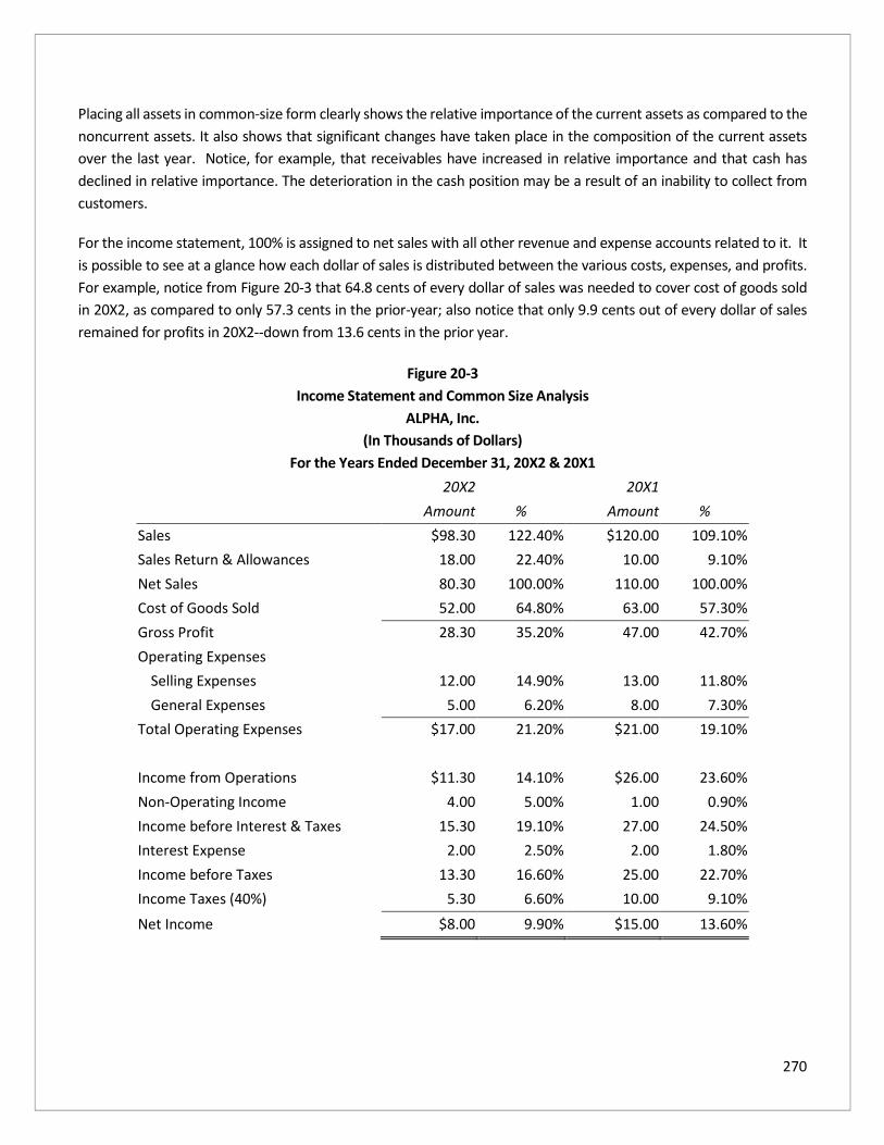
270

Placing all assets in common-size form clearly shows the relative importance of the current assets as compared to the

noncurrent assets. It also shows that significant changes have taken place in the composition of the current assets

over the last year. Notice, for example, that receivables have increased in relative importance and that cash has

declined in relative importance. The deterioration in the cash position may be a result of an inability to collect from

customers.

For the income statement, 100% is assigned to net sales with all other revenue and expense accounts related to it. It

is possible to see at a glance how each dollar of sales is distributed between the various costs, expenses, and profits.

For example, notice from Figure 20-3 that 64.8 cents of every dollar of sales was needed to cover cost of goods sold

in 20X2, as compared to only 57.3 cents in the prior-year; also notice that only 9.9 cents out of every dollar of sales

remained for profits in 20X2--down from 13.6 cents in the prior year.

Figure 20-3

Income Statement and Common Size Analysis

ALPHA, Inc.

(In Thousands of Dollars)

For the Years Ended December 31, 20X2 & 20X1

20X2 20X1

Amount % Amount %

Sales $98.30 122.40% $120.00 109.10%

Sales Return & Allowances 18.00 22.40% 10.00 9.10%

Net Sales 80.30 100.00% 110.00 100.00%

Cost of Goods Sold 52.00 64.80% 63.00 57.30%

Gross Profit 28.30 35.20% 47.00 42.70%

Operating Expenses

Selling Expenses 12.00 14.90% 13.00 11.80%

General Expenses 5.00 6.20% 8.00 7.30%

Total Operating Expenses $17.00 21.20% $21.00 19.10%

Income from Operations $11.30 14.10% $26.00 23.60%

Non-Operating Income 4.00 5.00% 1.00 0.90%

Income before Interest & Taxes 15.30 19.10% 27.00 24.50%

Interest Expense 2.00 2.50% 2.00 1.80%

Income before Taxes 13.30 16.60% 25.00 22.70%

Income Taxes (40%) 5.30 6.60% 10.00 9.10%

Net Income $8.00 9.90% $15.00 13.60%

271

You should also compare the vertical percentages of the business to those of the competition and to the industry

norms. Then you can determine how the company fares in the industry.

Ratio Analysis

Horizontal and vertical analysis compares one figure to another within the same category. It is also vital to compare

two figures applicable to different categories. This is accomplished by ratio analysis. In this section, you will learn

how to calculate the various financial ratios and how to interpret them. The results of the ratio analysis will allow you:

1. To appraise the position of a business,

2. To identify trouble spots that need attention, and

3. To provide the basis for making projections and forecasts about the course of future operations.

Think of ratios as measures of the relative health or sickness of a business. Just as a doctor takes readings of a patient's

temperature, blood pressure, heart rate, etc., you will take readings of a business's liquidity, profitability, leverage,

efficiency in using assets, and market value. Where the doctor compares the readings to generally accepted guidelines

such as a temperature of 98.6 degrees as normal, you make some comparisons to the norms.

To obtain useful conclusions from the ratios, you must make two comparisons:

Industry comparison will allow you to answer the question "how does a business fare in the industry?" You must

compare the company's ratios to those of competing companies in the industry or with industry standards (averages).

You can obtain industry norms from financial services such as Value Line, Dun and Bradstreet, and Standard and Poors.

Numerous online services such as Yahoo Finance and MSN Money, to name a few, provide these data.

Trend analysis will allow you to compare a given ratio for one company over several years to see the direction of

financial health or operational performance.

Financial ratios can be grouped into the following types:

• Liquidity

• Asset utilization (activity)

• Solvency (leverage and debt service)

• Profitability

• Market value

Each type is discussed below.

272

Liquidity

Liquidity is the firm's ability to satisfy maturing short-term debt. Liquidity is crucial to carrying out the business,

especially during periods of adversity. It relates to the short term, typically a period of one year or less. Poor liquidity

might lead to a higher cost of financing and inability to pay bills and dividends. The three basic measures of liquidity

are (a) net working capital, (b) the current ratio, and (c) the quick (acid-test) ratio.

Throughout our discussion, keep referring to Figures 20-1 and 22-2 to make sure you understand where the numbers

come from.

Net working capital equals current assets minus current liabilities. Net working capital for 20X2 is:

Net working capital = current assets - current liabilities

= $124 - $56

= $68

In 20X1, net working capital was $63. The rise over the year is favorable.

The current ratio equals current assets divided by current liabilities. The ratio reflects the company's ability to satisfy

current debt from current assets.

Current ratio = Current assets

Current liabilities

For 20X2, the current ratio is:

$124 $56

= 2.21

In 20X1, the current ratio was 2.26. The ratio's decline over the year points to a slight reduction in liquidity.

A more stringent liquidity test can be found in the quick (acid-test) ratio. Inventory and prepaid expenses are excluded

from the total of current assets, leaving only the more liquid (or quick) assets to be divided by current liabilities.

Acid-test ratio = Cash + marketable securities

Current liabilities

The quick ratio for 20X2 is:

$28+$21+$22 $56

= 1.27

In 20X1, the ratio was 1.34. A small reduction in the ratio over the period points to less liquidity.

The overall liquidity trend shows a slight deterioration as reflected in the lower current and quick ratios, although it is

better than the industry norms (see Figure 20-4 for industry averages). But a mitigating factor is the increase in net

working capital.

273

Asset Utilization

Asset utilization (activity, turnover) ratios reflect the way in which a company uses its assets to obtain revenue and

profit. One example is how well receivables are turning into cash. The higher the ratio, the more efficiently the

business manages its assets.

Accounts receivable ratios comprise the accounts receivable turnover and the average collection period.

The accounts receivable turnover provides the number of times accounts receivable are collected in the year. It is

derived by dividing net credit sales by average accounts receivable.

You can calculate average accounts receivable by the average accounts receivable balance during a period.

Accounts receivable turnover = Net credit sales

Average accounts receivable

For 20X2, the average accounts receivable is:

$21+$16 2

= $18.5

The accounts receivable turnover for 20X2 is:

$80.3 = 4.34

$18.5

In 20X1, the turnover was 8.46. There is a sharp reduction in the turnover rate pointing to a collection problem.

The average collection period is the length of time it takes to collect receivables. It represents the number of days

receivables are held.

Average collection period = 365 days

Accounts receivable turnover

In 20X2, the collection period is:

365 4.34

= 84.1 days

It takes this firm about 84 days to convert receivables to cash. In 20X1, the collection period was 43.1 days. The

significant lengthening of the collection period may be a cause for some concern. The long collection period may be a

result of the presence of many doubtful accounts, or it may be a result of poor credit management.

Inventory ratios are useful especially when a buildup in inventory exists. Inventory ties up cash. Holding large amounts

of inventory can result in lost opportunities for profit as well as increased storage costs. Before you extend credit or

lend money, you should examine the firm's inventory turnover and average age of inventory.

Inventory turnover = Cost of goods sold Average inventory

274

The inventory turnover for 20X2 is:

_$52_ $49.5

= 1.05

For 20X1, the turnover was 1.33.

Average age of inventory = 365 days

Inventory turnover

In 20X2, the average age is:

365 = 347.6 days

1.05

In the previous year, the average age was 274.4 days.

The reduction in the turnover and increase in inventory age points to a longer holding of inventory. You should ask

why the inventory is not selling as quickly.

The operating cycle is the number of days it takes to convert inventory and receivables to cash.

Operating cycle = average collection period + average age of inventory

In 20X2, the operating cycle is:

84.1 days + 347.6 days = 431.7 days

In the previous year, the operating cycle was 317.5 days. An unfavorable direction is indicated because additional

funds are tied up in noncash assets. Cash is being collected more slowly.

By calculating the total asset turnover, you can find out whether the company is efficiently employing its total assets

to obtain sales revenue. A low ratio may indicate too high an investment in assets in comparison to the sales revenue

generated.

Total asset turnover = Net sales

Average total assets

In 20X2, the ratio is:

$80.3 =

$80.3 = 0.37

($204 + $227) / 2 $215.5

In 20X1, the ratio was .57 ($110/$194.5). There has been a sharp reduction in asset utilization.

ALPHA, Inc. has suffered a sharp deterioration in activity ratios, pointing to a need for improved credit and inventory

management, although the 20X2 ratios are not far out of line with the industry averages (See Figure 20-4). It appears

that problems are inefficient collection and obsolescence of inventory.

275

Solvency

Solvency is the company's ability to satisfy long-term debt as it becomes due. You should be concerned about the

long-term financial and operating structure of any firm in which you might be interested. Another important

consideration is the size of debt in the firm's capital structure, which is referred to as financial leverage. (Capital

structure is the mix of the long term sources of funds used by the firm).

Solvency also depends on earning power; in the long run, a company will not satisfy its debts unless it earns profit. A

leveraged capital structure subjects the company to fixed interest charges, which contributes to earnings instability.

Excessive debt may also make it difficult for the firm to borrow funds at reasonable rates during tight money markets.

The debt ratio reveals the amount of money a company owes to its creditors. Excessive debt means greater risk to the

investor. (Equity holders come after creditors in bankruptcy.)

Note: How much debt is too much? The rule of thumb is: The debt portion should be less than 50%. All bankruptcies

arise from a company’s inability to meet its debt obligations, according to BankruptcyData.com).

The debt ratio is:

Debt ratio = Total liabilities

Total assets


$139 = 0.61

$227

The debt-equity ratio will show you if the firm has a great amount of debt in its capital structure. Large debts mean

that the borrower has to pay significant periodic interest and principal. Also, a heavily indebted firm takes a greater

risk of running out of cash in difficult times. The interpretation of this ratio depends on several variables, including

the ratios of other firms in the industry, the degree of access to additional debt financing, and stability of operations.

Debt – equity ratio = Total liabilities

Stockholders’ equity


$139 = 1.58

$88

In the previous year, the ratio was 1.55. the trend is relatively static.

276

Times interest earned (interest coverage ratio) tells you how many times the firm's before-tax earnings would cover

interest. It is a safety margin indicator in that it reflects how much of a reduction in earnings a company can tolerate.

Times interest earned = Income before interest and taxes

Interest expense

For 20X2, the ratio is:

$15.3 = 7.65

$2.0

In 20X1, interest was covered 13.5 times. The reduction in coverage during the period is a bad sign. It means that

fewer earnings are available to satisfy interest charges.

You must also note liabilities that have not yet been reported in the balance sheet by closely examining footnote

disclosure. For example, you should find out about lawsuits, non-capitalized leases, and future guarantees.

As shown in Figure 20-4, the company's overall solvency is poor, relative to the industry averages although it has

remained fairly constant. There has been no significant change in its ability to satisfy long-term debt. Note that

significantly less profit is available to cover interest payments.

Profitability

A company's ability to earn a good profit and return on investment is an indicator of its financial well-being and the

efficiency with which it is managed. Poor earnings have detrimental effects on the market price of stock and

dividends. Total dollar net income has little meaning unless it is compared to the input in getting that profit.

The gross profit margin shows the percentage of each dollar remaining once the company has paid for goods acquired.

A high margin reflects good earning potential.

Gross profit margin = Gross profit

Net sales


$28.3 = 0.35

$80.3

The ratio was .43 in 20X1. The reduction shows that the company now receives less profit on each dollar sales.

Perhaps a higher relative cost of merchandise sold is at fault.

Profit margin shows the earnings generated from revenue and is a key indicator of operating performance. It gives

you an idea of the firm's pricing, cost structure, and production efficiency.

Profit margin = Net income

Net sales

277

The ratio in 20X2 is:

$8.0 = 0.10

$80.3

For the previous year, the profit margin was .14. The decline in the ratio shows a downward trend in earning power.

(Note that these percentages are available in the common size income statement as given in Figure 20-3).

Return on investment is a prime indicator because it allows you to evaluate the profit you will earn if you invest in the

business. Two key ratios are the return on total assets and the return on equity.

The return on total assets shows whether management is efficient in using available resources to get profit.

Return on total assets = Net income

Average total assets

In 20X2, the return is:

$8.0 = 0.037

($227+$204)/2

In 20X1, the return was .077. There has been a deterioration in the productivity of assets in generating earnings.

The return on equity (ROE) reflects the rate of return earned on the stockholders' investment.

Return on common equity = Net income available to stockholders

Average stockholders’ equity

The return in 20X2 is:

$8.0 = 0.095

($88+$80)/2

In 20X1, the return was .207. There has been a significant drop in return to the owners.

The overall profitability of the company has decreased considerably, causing a decline in both the return on assets

and return on equity. Perhaps lower earnings were due in part to higher costs of short-term financing arising from

the decline in liquidity and activity ratios. Moreover, as turnover rates in assets go down, profit will similarly decline

because of a lack of sales and higher costs of carrying higher current asset balances. As indicated in Figure 20-4,

industry comparisons reveal that the company is faring very poorly in the industry.

278

Market Value

Market value ratios compare the company's stock price to its earnings (or book value) per share. Also included are

dividend-related ratios.

Earnings per share (EPS) is the ratio most widely watched by investors. EPS shows the net income per common share

owned. You must reduce net income by the preferred dividends to obtain the net income available to common

stockholders. Where preferred stock is not in the capital structure, you determine EPS by dividing net income by

common shares outstanding. EPS is a gauge of corporate operating performance and of expected future dividends.

EPS = Net income – preferred dividend

Common shares outstanding

EPS in 20X2 is:

$8,000 = $1.74

4,600 shares

For 20X1, EPS was $3.26. The sharp reduction over the year should cause alarm among investors. As you can see in

Figure 20-4, the industry average EPS in 20X2 is much higher than that of ALPHA, Inc. ($4.51 per share vs. $1.74 per

share).

The price/earnings (P/E) ratio, also called earnings multiple, reflects the company's relationship to its stockholders.

The P/E ratio represents the amount investors are willing to pay for each dollar of the firm's earnings. A high multiple

(cost per dollar of earnings) is favored since it shows that investors view the firm positively. On the other hand,

investors looking for value would prefer a relatively lower multiple (cost per dollar of earnings) as compared with

companies of similar risk and return.

Price/earnings ratio = Market price per share

Earnings per share

Assume a market price per share of $12 on December 31, 20X2, and $26 on December 31, 20X1. The P/E ratios are:

20X2:

$12 = 6.9

$1.74

20X1

$26 = 7.98

$3.26

279

From the lower P/E multiple, you can infer that the stock market now has a lower opinion of the business. However,

some investors argue that a low P/E ratio can mean that the stock is undervalued. Nevertheless, the decline over the

year in stock price was 54% ($14/$26), which should cause deep investor concern.

Book value per share equals the net assets available to common stockholders divided by shares outstanding. By

comparing it to the market price per share you can get another view of how investors feel about the business.

The book value per share in 20X2 is:

Book value per share = Total stockholders’ equity – preferred stock

Common shares outstanding

For 20X2:

$88,000 - 0 = $19.13

4,600

In 20X1, book value per share was $17.39.

The increased book value per share is a favorable sign because it indicates that each share now has a higher book

value. However, in 20X2, market price is much less than book value, which means that the stock market does not

value the security highly. In 20X1, market price did exceed book value, but there is now some doubt in the minds of

stockholders concerning the company. However, some analysts may argue that the stock is underpriced.

The price/book value ratio shows the market value of the company in comparison to its historical accounting value. A

company with old assets may have a high ratio whereas one with new assets may have a low ratio. Hence, you should

note the changes in the ratio in an effort to appraise the corporate assets.

The ratio equals:

Price / book value = Market price per share Book value per share


$12 = .63

$19.13

In 20X1, the ratio was 1.5. The significant drop in the ratio may indicate a lower opinion of the company in the eyes

of investors. The market price of stock may have dropped because of a deterioration in liquidity, activity, and

profitability ratios. The major indicators of a company's performance are intertwined (i.e., one affects the other) so

that problems in one area may spill over into another. This appears to have happened to the company in our example.

Dividend ratios help you determine the current income from an investment. Two relevant ratios are:

280

Dividend yield = Dividends per share

Market price per share

Dividend payout = Dividends per share Earnings per share

There is no such thing as a "right" payout ratio. Stockholders look unfavorably upon reduced dividends because it is a

sign of possible deteriorating financial health. However, companies with ample opportunities for growth at high rates

of return on assets tend to have low payout ratios.

Comprehensive Illustration

As indicated in the chapter, a single ratio or a single group of ratios is not adequate for assessing all aspects of the

firm's financial condition. Figure 20-4 summarizes the 20X1 and 20X2 ratios calculated in the previous sections, along

with the industry average ratios for 20X2. The figure also shows the formula used to calculate each ratio. The last

three columns of the figure contain subjective assessments of ALPHA's financial condition, based on trend analysis

and 20X2 comparisons to the industry norms. (5-year ratios are generally needed for trend analysis to be more

meaningful, however.)

281

Figure 20-4

ALPHA, Inc.

Summary of Financial Ratios - Trend and Industry Comparisons

Evaluationb

Ratios Definitions 20X1 20X2 Industrya Ind Trend Overall

LIQUIDITY

Net working capital Current assets - current liabilities 63 68 56 good good good

Current Ratio Current assets/current liabilities 2.26 2.21 2.05 OK OK OK

Quick (Acid-test) ratio (Cash + marketable securities + accounts receivable)/current liabilities 1.34 1.27 1.11 OK OK OK

ASSET UTILIZATION

Accounts receivable turnover Net credit sales/average accounts receivable 8.46 4.34 5.5 OK poor poor

Average collection period 365 days/accounts receivable turnover (days) 43.1 84.1 66.4 OK poor poor

Inventory turnover Cost of goods sold/average inventory 1.33 1.05 1.2 OK poor poor

Average age of inventory 365 days/inventory turnover (days) 274.4 347.6 N/A N/A poor poor

Operating cycle Average collection period + average age of inventory (days) 317.5 431.7 N/A N/A poor poor

Total asset turnover Net sales/average total assets 0.57 0.37 0.44 OK poor poor

SOLVENCY

Debt ratio Total liabilities/total assets 0.61 0.61 N/A N/A OK OK

Debt-equity ratio Total liabilities/stockholders' equity 1.55 1.58 1.3 poor poor poor

Times interest earned Income before interest and taxes/interest expense (times) 13.5 7.65 10 OK poor poor

PROFITABILITY

Gross profit margin Gross profit/net sales 0.43 0.35 0.48 poor poor poor

Profit margin Net income/net sales 0.14 0.1 0.15 poor poor poor

Return on total assets Net income/average total assets 0.077 0.037 0.1 poor poor poor

Return on equity(ROE) Earnings available to common stockholders/ avg. stockholders' equity 0.207 0.095 0.27 poor poor poor

282

Figure 20-4

ALPHA, Inc.

Summary of Financial Ratios - Trend and Industry Comparisons

Evaluationb

Ratios Definitions 20X1 20X2 Industrya Ind Trend Overall

MARKET VALUE

Earnings per share(EPS) (Net income -preferred dividend)/common shares outstanding 3.26 1.74 4.51 poor poor poor

Price/earnings (P/E) ratio Market price per share/EPS 7.98 6.9 7.12 OK poor poor

Book value per share

(Total stockholders' eqty - Preferred stock)/ common shrs

outstanding 17.39 19.13 N/A N/A good good

Price/book value ratio Market price per share/book value per share 1.5 0.63 N/A N/A poor poor

Dividend yield Dividends per share/market price per share

Dividend payout Dividends per share/EPS

(a) Obtained from sources not included in this chapter

(b) Represent subjective evaluation

283

By appraising the trend in the company's ratios from 20X1 to 20X2, we see from the drop in the current and quick

ratios that there has been a slight detraction in short-term liquidity, although they have been above the industry

averages. But working capital has improved. A material deterioration in the activity ratios has occurred, indicating that

improved credit and inventory policies are required. They are not terribly alarming, however, because these ratios are

not way out of line with industry averages. Also, the total utilization of assets, as indicated by the total asset turnover,

shows a deteriorating trend.

Leverage (amount of debt) has been constant. However, there is less profit available to satisfy interest charges.

ALPHA's profitability has deteriorated over the year. In 20X2, it is consistently below the industry average in every

measure of profitability. In consequence, the return on the owner's investment and the return on total assets have

gone down. The earnings decrease may be partly due to the firm's high cost of short-term financing and partly due to

operating inefficiency. The higher costs may be due to receivable and inventory difficulties that forced a decline in

the liquidity and activity ratios. Furthermore, as receivables and inventory turnover less, profit will fall off from a lack

of sales and the costs of carrying more in current asset balances.

The firm's market value, as measured by the price/earnings (P/E) ratio, is respectable as compared with the industry.

But it shows a declining trend.

In summary, it appears that the company is doing satisfactorily in the industry in many categories. The 20X1-20X2

period, however, seems to indicate that the company is heading for financial trouble in terms of earnings, activity,

and short-term liquidity. The business needs to concentrate on increasing operating efficiency and asset utilization.

Conclusion

Financial statement analysis is an attempt to work with reported financial figures in order to determine a

company’s financial strengths and weaknesses. Most analysts favor certain ratios and ignore others. Each ratio

should be compared to industry norms and analyzed in light of past trends. Financial analysis also calls for an

awareness of the impact of inflation and deflation on reported income. Ratio analysis provides useful information

regarding the efficiency of operations and the stability of the financial condition. Nevertheless, it has several

inherent limitations, such as firms using different accounting and operating policies, multiple lines of businesses,

and different sources of information. Each of these factors impairs the comparability of financial statement

amounts and the ratios derived from them.

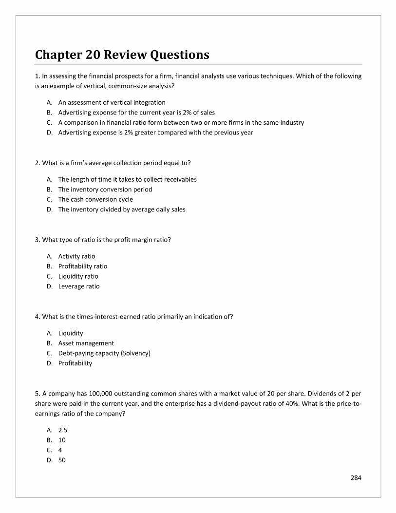
284


1. In assessing the financial prospects for a firm, financial analysts use various techniques. Which of the following

is an example of vertical, common-size analysis?

A. An assessment of vertical integration

B. Advertising expense for the current year is 2% of sales

C. A comparison in financial ratio form between two or more firms in the same industry

D. Advertising expense is 2% greater compared with the previous year

2. What is a firm’s average collection period equal to?

A. The length of time it takes to collect receivables

B. The inventory conversion period

C. The cash conversion cycle

D. The inventory divided by average daily sales

3. What type of ratio is the profit margin ratio?

A. Activity ratio

B. Profitability ratio

C. Liquidity ratio

D. Leverage ratio

4. What is the times-interest-earned ratio primarily an indication of?

A. Liquidity

B. Asset management

C. Debt-paying capacity (Solvency)

D. Profitability

5. A company has 100,000 outstanding common shares with a market value of 20 per share. Dividends of 2 per

share were paid in the current year, and the enterprise has a dividend-payout ratio of 40%. What is the price-to-

earnings ratio of the company?

A. 2.5

B. 10

C. 4

D. 50

285

6. Horn Company paid out one-half of last year's earnings in dividends. Horn’s earnings increased by 20%, and the

amount of its dividends increased by 15% in the current year. What was Horn's dividend payout ratio for the

current year?

A. 50%

B. 57.5%

C. 47.9%

D. 78%

7. Financial ratio analysis has no limitation when it comes to comparing financial fitness among firms. True or

False?

286

Glossary Accelerated depreciation A depreciation method wherein the depreciation charges decrease with time.

Accounting profit Net income or earnings figures shown on the income statement.

Accounting equation An expression of the equivalency in dollar amounts of assets and liabilities and equity in double-

entry accounting often stated as Assets = Liabilities + Owners' Equity.

Accounts receivable turnover Annual credit sales divided by average accounts receivable.

Accumulated Taxable Income The firm's taxable income less dividends paid and accrued during the year, and less

an accumulated earnings credit.

Accrual basis accounting Recognition of revenue when earned and expenses when incurred.

After-tax cash flow The net cash flow (cash revenue less cash expenses) after taxes have been subtracted. It is the

cash flow generated from operations.

Amortization The spreading out of costs over a period of time.

Amortized loan A loan that is paid off in periodic equal installments and includes varying portions of principal and

interest during its term.

Analysis of variances (variance analysis) An analysis and investigation of causes for variances between standard costs

and actual costs. A variance is considered favorable if actual costs are less than standard costs; it is unfavorable if

actual costs exceed standard costs. Unfavorable variances are the ones that need further investigation for their

causes, so corrective action may be taken.

Annual report A glossary magazine-style report that companies must send to shareholders annually. It includes the

company's financial statements.

Annuity A series of equal periodic payments or receipts.

Annuity due An annuity where payments or receipts occur at the beginning of the period.

Asset turnover The sales divided by average total assets, revealing the efficiency of assets in generating revenue.

Assets The resources owned by the firm.

Balance sheet equation See Accounting Equation.

Balance sheet A table that shows the status of a company's assets, liabilities, and owners' equity as of a given date.

287

Bankers' Acceptances A draft (order to pay) drawn on a specific bank by a seller of goods in order to obtain

payment for goods that have been shipped (sold) to a customer. The customer maintains an account with that

specific bank.

Bank Wire. A private wire service used and supported by approximately 250 banks in the United States for

transferring funds, exchanging credit information, or effecting securities transactions.

Bond A form of interest-bearing note payable, or simply a corporate long term IOU.

Book value per share The worth of each share of stock per the books based on historical cost.

Break-even analysis A branch of cost-volume-profit (CVP) analysis that determines the break-even sales, which is the

level of sales where total costs equal total revenue. At the break-even point, there is no profit or loss.

Break-even point The level of sales where total costs equal total revenue.

Budget A quantitative plan of activities and programs expressed in terms of assets, liabilities, revenues, and expenses.

See also Master Budget.

Capital budget A budget or plan of proposed acquisitions and replacements of long-term assets and their financing.

A capital budget is developed using a variety of capital budgeting techniques such as the discount cash flow method.

Capital budgeting The process of making long-term planning decisions for capital investments.

Capital structure Composition of common stock, preferred stock, retained earnings, and long-term debt maintained

by the business entity in financing its assets.

Capital rationing The selection of the mix of acceptable projects that provides the highest overall net present value

of future cash flows when a company has a limit on the budget for capital spending.

Cash budget A budget for cash planning and control that presents anticipated cash inflow and cash outflow for a

specified time period. The cash budget helps the owner keep cash balances in reasonable relationship to needs. It

assists in avoiding idle cash and possible cash shortages. The cash budget shows beginning cash, cash receipts, cash

payments, and ending cash.

Cash flow (1) Cash receipts minus cash disbursements from a given operation or asset for a given period. Cash flow

and cash inflow are often used interchangeably. (2) The monetary value of the expected benefits and costs of a

project. It may be in the form of cash savings in operating costs or the difference between additional dollars received

and additional dollars paid out for a given period.

Cash flow statement A statement showing from what sources cash has come into the business and on what the cash

has been spent. Cash flow is broken down into operating, investing, and financing activities.

Cash basis accounting Method of recognizing revenue and expenses when cash received or paid.

Chart of accounts A list of account names and numbers found in the general ledger and arranged in the order in

which they customarily appear in the financial statements.

288

Chief Financial Officer (CFO) Executive who directs all financial aspects of the business.

Collection period The number of days it takes to collect accounts receivable. It equals 365 days divided by the

accounts receivable turnover. The collection period should be compared to the terms of sale.

Commercial Paper Short-term unsecured promissory notes sold by large businesses in order to raise cash. Unlike

most other money market instruments, commercial paper has no developed secondary market.

Common costs A cost shared by different departments, products, or jobs. Also called joint costs or indirect costs.

Compensating Balance A balance of a given amount that the firm maintains in its demand deposit account. It may

be required by either a formal or informal agreement with the firm's commercial bank. Such balances are usually

required by the bank (1) on the unused portion of a loan commitment, (2) on the unpaid portion of an outstanding

loan, or (3) in exchange for certain services provided by the bank, such as check-clearing or credit information.

These balances raise the effective rate of interest paid on borrowed funds.

Compounding. The process of determining the future value of a payment or series of payments when applying

the concept of compound interest.

Compound Interest. The situation in which interest paid on the investment during the first period is added to the

principal and, during the second period, interest is earned on the original principal plus the interest earned during

the first period.

Concentration Bank. A bank where the firm maintains a major disbursing account.

Comprehensive budget See master budget.

Constraining (limiting) factor The item or factor that restricts or limits the production or sale of a given product.

Virtually all firms suffer from one or more constraining factors. Examples of constraining factors include limited

machine-hours, labor-hours and shortage of materials and skilled labor. Other limiting factors may be cubic feet of

display or warehouse space or working capital.

Contribution margin (CM) The difference between sales and the variable costs of the product or service, also called

marginal income. It is the amount of money available to cover fixed costs and generate profits.

Contribution margin (CM) ratio The contribution margin (cm) as a percentage of sales.

Contribution (margin) income statement An income statement that organizes the cost by behavior. It shows the

relationship between variable costs and fixed costs, regardless of the functions a given cost item is associated with.

Contribution approach to pricing An approach to pricing a special order. This situation occurs because a company

often receives a non-routine, special order for its products at lower prices than usual. In normal times, the company

may refuse such an order since it will not yield a satisfactory profit. If times are bad or when there is idle capacity, an

order should be accepted if the incremental revenue exceeds the incremental costs involved.

Controller Chief accounting executive of an organization. The controller is in charge of the Accounting Department.

The principal functions of the controller are (1) planning for control; (2) financial reporting and interpreting; (3) tax

289

administration; (4) management audits and development of accounting systems; (5) internal audits.

Conversion costs The sum of the costs of direct labor and factory overhead.

Cost center The unit within the organization in which the manager is responsible only for costs. A cost center has no

control over sales or over the generating of revenue. An example is the production department of a manufacturing

company. The performance of the cost center is evaluated by comparing actual costs to budgeted costs.

Cost of capital The minimum rate of return that is necessary to keep the market value (or stock price) of a firm.

Cost behavior analysis An analysis of mixed costs. Mixed costs must be separated into the variable and fixed elements

in order to be included in a variety of business planning analyses such as cost-volume-profit (CVP) analysis.

Cost control The steps taken by management to assure that the cost objectives set down in the planning stage are

attained and to assure that all segments of the organization function in a manner consistent with its policies. For

effective cost control, most organizations use standard cost systems, in which the actual costs are compared against

standard costs for performance evaluation and the deviations are investigated for remedial actions. Cost control is

also concerned with feedback that might change any or all of the future plans, the production method, or both.

Cost-volume formula A cost function in the form of y = a + bx. For example, the cost-volume formula for factory

overhead is y=$200 + $10x where y=estimated factory overhead and x=direct labor hours, which means that the

factory overhead is estimated to be $200 fixed, plus $10 per hour of direct labor. Cost analysts use the formula for

cost prediction and flexible budgeting purposes.

Cost-volume-profit (CVP) analysis An analysis that deals with how profits and costs change with a change in volume.

It looks at the effects on profits of changes in such factors as variables costs, fixed costs, selling prices, volume, and

mix of products sold.

Credit entry Transaction recorded on the right-hand side of an account.

Current ratio Current assets divided by current liabilities.

Debit entry Transaction recorded on the left-hand side of an account.

Debt-equity ratio Total liabilities divided by total stockholders' equity.

Departmental rate A predetermined factory overhead rate for each production department.

Depreciation The procedure of spreading out the acquisition cost of fixed assets (such as machinery and equipment)

to each of the time periods in which they are utilized.

Direct materials budget A budget that shows how much material will be required for production and how much

material must be bought to meet this production requirement. The purchase depends on both the expected usage of

materials and inventory levels.

Direct labor budget A schedule for expected labor costs. The expected labor cost is dependent upon expected

production volume (production budget). Labor requirements are based on production volume multiplied by direct

290

labor hours per unit. Direct labor hours needed for production is then multiplied by direct labor cost per hour to derive

budgeted direct labor costs.

Discounted cash flow (DCF) techniques Methods of selecting and ranking investment proposals such as the net

present value (NPV) and internal rate of return (IRR) methods where the time value of money is taken into account.

Discretionary (fixed) costs The fixed costs that change because of managerial decisions, also called management

(fixed) costs or programmed (fixed) costs. Examples of this type of fixed costs are advertising, training, and research

and development.

Double-entry bookkeeping A method of accounting that recognizes the duality of a transaction such that any change

in one account also causes a change in another account.

Earnings A synonym for net income or profit after taxes.

Earnings per share (EPS) Net income after taxes available to common shareholders on a per-share basis.

Economic profit The same as cash inflows

Equity The difference between the assets of an entity and its liabilities. Also called net worth, owners' equity, or

stockholders' equity.

Facilities investment budget A budget plan prepared for individual facility expenditure projects. The time span of this

budget depends upon the project. Capital expenditures to be budgeted include replacement, acquisition, or

construction of plants and major equipment. See also Capital Budgeting.

Factoring of Accounts Receivable. The outright sale of a firm's accounts to another party (the factor) without

recourse. The factor, in turn, bears the risk of collection.

Factory overhead budget A schedule of all expected manufacturing costs except for direct material and direct labor.

Factory overhead items include indirect material, indirect labor, factory rent, and factory insurance.

Financial leverage A portion of a firm's assets financed with debt instead of equity.

Financial Accounting Standards Board (FASB) The seven-member board which currently has the authority to

formulate and issue pronouncements of generally accepted accounting principles.

Fixed cost A cost that remains the same each period in the short run regardless of activity. Examples are rent, interest,

insurance, and property taxes.

Fixed budget See Static Budget.

Flexible budget formula See Cost-Volume Formula.

Flexible budget A budget based on cost-volume relationships and developed for the actual level of activity. It is an

extremely useful tool for comparing the actual cost incurred to the cost allowable for the activity level achieved.

Fundamental equation of accounting See Accounting Equation.

291

General ledger A grouping of the accounts in which the transactions of an entity are recorded.

Generally Accepted Accounting Principles (GAAP) Rules, regulations, standards, conventions, and pronouncements

used as a basis for financial reporting, and in the preparation of financial statements.

Gross profit margin The ratio of gross profit to net sales. A high gross profit margin is a positive sign since it shows

the business is earning an attractive return over the cost of its merchandise sold.

Illiquid 1. Lacking enough liquid assets, like cash and marketable securities, to cover short-term obligations. 2.

Current liabilities exceed current assets.

Income statement A table that details a company's revenue, expenses, and profit or loss for a given period.

Industry norm A typical ratio for the industry based on averaging companies' values.

Insolvency The failure of a company to meet its obligations as they become due. An analysis of insolvency

concentrates on the operating and capital structure of the business. The proportion of long-term debt in the capital

structure must also be considered.

Internal rate of return (IRR) The rate of return on a proposal that equates the initial investment with the present

value of future cash inflows.

Inventory turnover The number of times inventory is sold during the year. It equals the cost of goods sold divided

by the average dollar balance. Average inventory equals the beginning and ending balances divided by two.

Investment center A responsibility center within an organization that has control over revenue, cost and investment

funds. It is a profit center whose performance is evaluated on the basis of the return earned on invested capital.

Joint products The products that have a relatively significant sales value when two or more types of products are

produced simultaneously from the same input by a joint process. For example, gasoline, fuel oil, kerosene, and

paraffin are the joint products that are produced from crude oil.

Joint costs All the common manufacturing costs incurred prior to the point, referred to as the split-off point, where

the joint products are identified as individual products.

Journal A book in which all business transactions are recorded in chronological order.

Just-In-Time (JIT) A demand-pull system where demand for customer output (not plans for using input resources)

triggers production. Production activities are "pulled", not "pushed," into action.

Labor efficiency variance The difference between the amount of labor time that should have been used and the labor

that was actually used, multiplied by the standard rate.

Labor rate variance A deviation from standard in the average hourly rate paid to workers.

Least-squares method The method that fits a line in such a way that the sum of squared distances from the data

points to the line is minimized.

292

Ledger Book in which all accounts of the business are maintained.

Liabilities Obligations of the firm to outside creditors such as lenders and bondholders.

Liquidity The ability of current assets to meet current liabilities when due.

Mail Float Funds tied up during the time that elapses from the moment a customer mails his remittance check

until the firm begins to process it.

Management by exception A management concept or policy by which management devotes its time to investigating

only those situations in which actual results differ significantly from planned results. The idea is that management

should spend its valuable time concentrating on the more important items (such as the shaping of the company's

future strategic course).

Master (comprehensive) budget A plan of activities expressed in monetary terms of the assets, equities, revenues,

and costs that will be involved in carrying out the plans. It is a set of projected or planned financial statements.

Materials quantity (usage) variance The difference between the actual quantity of materials used in production and

the standard quantity of materials allowed for actual production, multiplied by the standard price per unit.

Materials price variance The difference between what is paid for a given quantity of materials and what should have

been paid, multiplied by the actual quantity of materials used.

Mixed costs The costs that vary with changes in volume but, unlike variable costs, do not vary in direct proportion,

also called semi-variable costs.

Modified Accelerated Cost Recovery System (MACRS) The system used in computing annual depreciation for assets

acquired in 1987.

Net present value (NPV) The difference between the present value of cash inflows generated by the project and the

amount of the initial investment.

Notes to the financial statements Important information supplementing the financial statements.

Operating cycle The average time period between buying inventory and receiving cash proceeds from its eventual

sale. It is determined by adding the number of days inventory is held and the collection period for accounts receivable.

Operating leverage The degree to which the firm chooses to lock in fixed costs other than financing costs.

Operational (operating) budget A budget that embraces the impacts of operating decisions. It contains forecasts of

sales, net income, the cost of goods sold, selling and administrative expenses, and other expenses.

Opportunity cost The revenue forfeited by rejecting an alternative use of time or facilities.

Ordinary annuity An annuity where payments or receipts occur at the end of the period.

Out-of-pocket cost The actual cash outlays made during the period for payroll, advertising, and other operating

expenses. Depreciation is not an out-of-pocket cost since it involves no current cash expenditure.

293

Owners' equity The value of the firm to its owners. It is the difference between assets and liabilities. See also Equity.

Payback period The number of years it takes to recover your initial investment. The payback period equals the initial

investment divided by the annual cash inflow.

Predetermined overhead rates An overhead rate, based on budgeted factory overhead cost and budgeted activity

that is established before a period begins.

Preferred stock An equity instrument that promises to pay its holders a fixed dividend.

Present value The current worth of future sums of money.

Pro forma income statement A budgeted income statement.

Pro forma balance sheet A budgeted balance sheet.

Product mix See Sales Mix.

Production budget A schedule for expected units to be produced. It sets forth the units expected to be manufactured

to satisfy budgeted sales and inventory requirements. The expected production volume is determined by adding the

desired ending inventory to planned sales and then subtracting beginning inventory.

Profit planning A process of developing a profit plan which outlines the planned sales revenues and expenses and

the net income or loss for a time period. Profit planning requires the preparation of a master budget and various

analyses for risk and "what-if" scenarios. Tools for profit planning include the cost-volume-profit (CVP) analysis and

budgeting.

Profit margin The ratio of net income to net sales. It reveals the entity's ability to generate profit at a given sales

level. The ratio gives the owner an indicator of the operating efficiency and pricing strategy of the business.

Profit-volume chart A chart that determines how profits vary with changes in volume.

Profitability index The ratio of the total present value of future cash inflows to the initial investment.

Projected (budgeted) income statement A summary of various component projections of revenues and expenses for

the budget period. It indicates the expected net income for the period.

Projected (budgeted) balance sheet A schedule for expected assets, liabilities, and stockholders' equity. It projects a

company's financial position as of the end of the budgeting year. Reasons for preparing a budgeted balance sheet

follow: (1) discloses unfavorable financial condition that management may want to avoid; (2) serves as a final check

on the mathematical accuracy of all other budgets; and (3) highlights future resources and obligations.

Quick ratio Also called acid-test ratio, the most liquid current assets (cash, marketable securities, accounts receivable)

divided by current liabilities.

Rate of return on investment (ROI) 1. For the company as a whole, net income after taxes divided by invested capital.

2. For the segment of an organization, net operating income divided by operating assets. 3. For capital budgeting

294

purposes, also called simple, accounting, or unadjusted rate of return, expected future net income divided by initial

(or average) investment.

Relevant cost The expected future cost that will differ between the alternatives being considered.

Residual income (RI) The operating income which an investment center is able to earn above some minimum return

on its assets. It equals operating income less the minimum rate of return times total assets.

Responsibility accounting The collection, summarization, and reporting of financial information about various

decision centers (responsibility centers) throughout an organization; also called activity accounting or profitability

accounting.

Responsibility center A unit in the organization which has control over costs, revenues, or investment funds. For

accounting purposes, responsibility centers are classified as cost centers, revenue centers, profit centers, and

investment centers, depending on what each center is responsible for.

Retained earnings The amount of income realized and retained since the inception of the entity less dividends paid

out to shareholders.

Return The reward for making an investment in the form of earnings and appreciation in value.

Risk 1. Variability about income, returns, or another financial variable. 2. The possibility of losing value.

Risk-return trade-off A comparison of the expected return from an investment with the risk associated with it. The

higher the risk undertaken, the more ample the return. Conversely, the lower the risk, the more modest the return.

Rule of OPM The use of other people's money (OPM) to magnify potential returns from the business. It is hoped that

investment through leverage will earn a rate of return greater than the costs of borrowing. Also called trading on the

equity.

Sales mix The relative proportions of the product sold.

Sales budget An operating plan for a period expressed in terms of sales volume and selling prices for each class of

product or service. Preparation of a sales budget is the starting point in budgeting since sales volume influences nearly

all other items.

Sales forecasting A projection or prediction of future sales. It is the foundation for the quantification of the entire

business plan and a master budget. Sales forecasts serve as a basis for planning.

Scatter diagram A plot of data points in an X-Y graph.

Segmented reporting The process of reporting activities of various segments of an organization such as divisions,

departments, product lines, services, sales territories, or customers.

Spontaneous Financing The trade-credit and other accounts payable that arise "spontaneously" in the firm's

day-to-day operations.

295

Spreadsheet A working paper having numbers in rows and columns.

Standard labor rate The standard rate for direct labor that would include not only base wages earned but also an

allowance for fringe benefits and other labor-related costs.

Standard cost system A system by which production activities are recorded at standard costs and variances from

actual costs are isolated.

Standard materials price The standard price per unit for direct materials. It reflects the final, delivered cost of the

materials, net of any discounts taken.

Standard hours allowed The standard time that should have been used to manufacture actual units of output during

a period. It is obtained by multiplying actual units of production by the standard labor time.

Standard A quantitative expression of a performance objective, such as standard hours of labor allowed for actual

production or a standard purchase price of materials per unit. Sometimes the terms standard and budget are used

interchangeably.

Standard quantity allowed The standard amount of materials that should have been used to manufacture units of

output during a period. It is obtained by multiplying actual units of production by the standard material quantity per

unit.

Standard costs Production or operating costs that are carefully predetermined. A standard cost is a target cost that

should be attained.

Static (fixed) budget A budget based on the anticipated output level rather than on the actual attained output level.

Term Loans. Loans that have maturities of one to ten years and are repaid in periodic installments over

the life of the loan. Term loans are usually secured by a chattel mortgage on equipment or a mortgage on

real property.

The Du Pont formula The breakdown of return on investment (ROI) into profit margin and asset turnover.

Time value of money The value of money at different time periods. As a rule, one dollar today is worth more than

one dollar tomorrow. The time value of money is a critical consideration in financial decisions.

Treasurer Financial officer in a firm who deals with money problems.

Turnover The number of times an asset, such as inventory, turns over during an accounting period.

Variance In the cost analysis, the deviation between the actual cost and the standard cost.

Venture Capitalists Investors interested in supplying the capital to particularly high-risk situations, such

as start-ups or firms denied conventional financing.

Working Capital A concept traditionally defined as a firm's investment in current assets. Net working capital refers

to the difference between current assets and current liabilities

296

Index

Accelerated depreciation, 286

Accounting equation, 286

Accrual basis accounting, 286

Amortization, 286

Balance sheet, 255, 286

Break-even analysis, 34, 41, 287, 303

Break-even point, 287

Capital budget, 287

Cash budget, 73, 287

Cash flow statement, 287

Commercial Paper, 199, 288

Contribution margin, 25, 26, 27, 28, 29, 31, 32, 41, 46,

50, 51, 52, 122, 177, 178, 288, 301, 319

Controller, 5, 8, 14, 288, 298

Cost control, 289

Cost-volume-profit, 33, 289

Current ratio, 289

Debt-equity ratio, 281, 289

Depreciation, 45, 66, 85, 146, 149, 151, 152, 153, 154,

289, 292, 316

Earnings per share, 235, 278, 282, 290

Factoring, 108, 200, 290

Fixed cost, 19, 26, 27, 28, 30, 36, 46, 290, 301

General ledger, 291

Income statement, 255, 261, 291

Internal rate of return, 144, 147, 291, 316

Joint products, 291

Labor rate variance, 291

Modified Accelerated Cost Recovery System, 153, 292

Net present value, 144, 146, 147, 229, 292

Operating leverage, 41, 292

Opportunity cost, 23, 101, 111, 292, 299

Payback period, 144, 145, 293

Present value, 129, 131, 142, 147, 207, 211, 293

Production budget, 73, 293

Profit margin, 276, 281, 293, 328

Quick ratio, 293

Relevant cost, 294

Residual income, 43, 182, 183, 189, 294, 302, 319,

320

Responsibility accounting, 172, 188, 294, 318

Responsibility center, 294

Sales budget, 73, 294

Segmented reporting, 294

Standard cost system, 295

Standard costs, 21, 90, 295, 307

Time value of money, 125, 295

297

Working Capital, 92, 295

298

Review Question Answers

Chapter 1 Review Answers

1. Which of the following items would not normally fall within the realm of the Controller?

A. Incorrect. The preparation of tax returns is s typical responsibility of the controller.

B. Correct. Controllers are usually in charge of budgeting, accounting, accounting reports, and related

controls. Treasures are most often involved with control over cash receivables, short-term investments,

financing, and insurance. Thus, treasurers rather than controllers are concerned with investor relations.

C. Incorrect. External reporting is a function of the controller.

D. Incorrect. The accounting system helps to safeguard assets.

2. The treasury function is usually NOT concerned with which of the following activities?

A. Correct. Treasurers are usually concerned with investing cash and near-cash assets, the provision of

capital, investor relations, insurance, etc. Controllers, on the other hand, are responsible for the reporting

and accounting activities of an organization, including financial reporting.

B. Incorrect. Short-term financing lies within the normal range of a treasurer's functions.

C. Incorrect. The treasurer has custody of assets.

D. Incorrect. Credit operations are often within the treasurer's purview.

3. In which legal form of business organization do the owners of the business enjoy limited liability?

A. Incorrect. General partners share profits and losses of the venture. Debts of a partnership are ultimately

the debts of the individual general partners.

B. Incorrect. A sole proprietorship is owned by one person. The sole proprietor is personally liable for all

debts.

C. Correct. Shareholders of a corporation own an equity interest in the underlying net assets of the

corporation and are entitled to share in its profits. Unlike a sole proprietor or a general partner, the

shareholder is not subject to liability beyond his/her investment.

D. Incorrect. An oligopoly is not a legal form of business organization.

299


1. When a decision is made in an organization, it is selected from a group of alternative courses of action. What is

the name for the loss associated with NOT choosing the alternative that maximizes the benefit to the company?

A. Incorrect. Net realizable value is the value of an asset net of any disposal costs.

B. Incorrect. Expected value is a weighted average of potential outcomes with weights being probabilities.

C. Correct. Opportunity costs include the net revenue foregone by rejecting an alternative. For example, if

you have the choice of using your department's capacity to produce an extra 10,000 units or renting it out

for $20,000, the opportunity cost of using the capacity is $20,000.

D. Incorrect. An incremental cost is the additional cost of selecting one option rather than another.

2. Which of the following statements is TRUE for controllable costs?

A. Incorrect. Periodic appropriation decisions that have no well-specified function relating inputs to outputs

apply to discretionary costs.

B. Correct. Controllable costs are those costs over which a manager has direct control (e.g., advertising if it

is at the discretion of the manager). All costs are controllable, but they are controlled at different

management levels; e.g., the decision to build another plant is made at a higher level of management

than the decision to buy office supplies.

C. Incorrect. Property, plant, and equipment costs are committed costs.

D. Incorrect. Engineered costs result from a measured relationship between inputs and outputs.

3. What are incremental costs?

A. Correct. Incremental (differential) costs are determined by calculating the difference in costs between

two or more alternatives. For example, if the direct labor costs for products A and B are $10,000 and

$15,000, respectively, the incremental cost is $5,000.

B. Incorrect. Opportunity cost is the profit forgone by selecting one choice instead of another.

C. Incorrect. A fixed cost is incurred even though no output is produced.

D. Incorrect. Common or joint costs are not allocable among the possible choices.

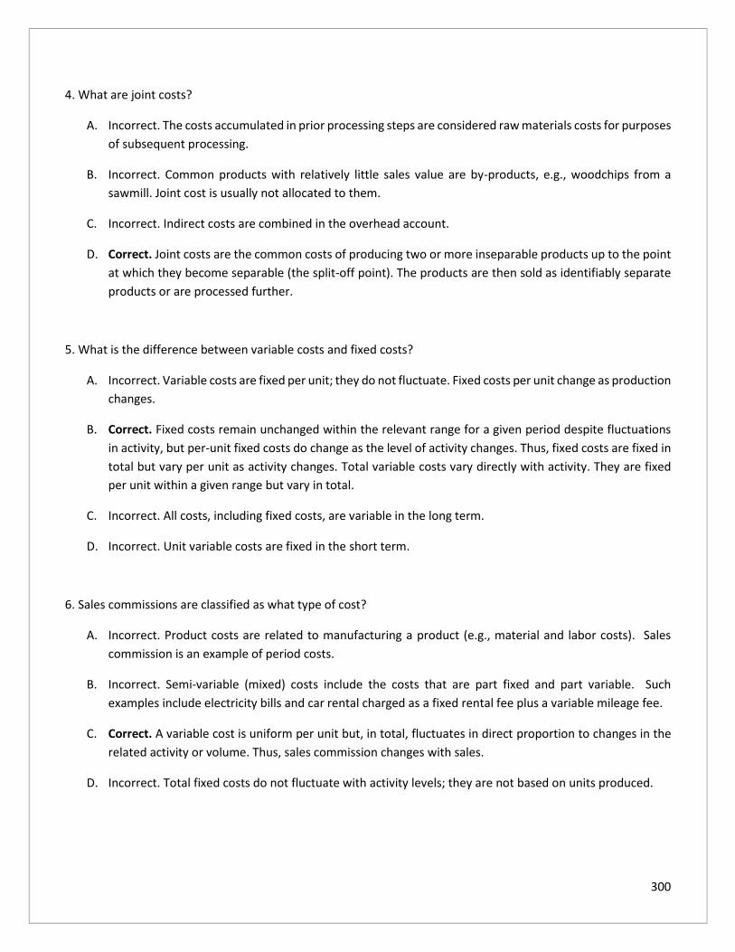
300

4. What are joint costs?

A. Incorrect. The costs accumulated in prior processing steps are considered raw materials costs for purposes

of subsequent processing.

B. Incorrect. Common products with relatively little sales value are by-products, e.g., woodchips from a

sawmill. Joint cost is usually not allocated to them.

C. Incorrect. Indirect costs are combined in the overhead account.

D. Correct. Joint costs are the common costs of producing two or more inseparable products up to the point

at which they become separable (the split-off point). The products are then sold as identifiably separate

products or are processed further.

5. What is the difference between variable costs and fixed costs?

A. Incorrect. Variable costs are fixed per unit; they do not fluctuate. Fixed costs per unit change as production

changes.

B. Correct. Fixed costs remain unchanged within the relevant range for a given period despite fluctuations

in activity, but per-unit fixed costs do change as the level of activity changes. Thus, fixed costs are fixed in

total but vary per unit as activity changes. Total variable costs vary directly with activity. They are fixed

per unit within a given range but vary in total.

C. Incorrect. All costs, including fixed costs, are variable in the long term.

D. Incorrect. Unit variable costs are fixed in the short term.

6. Sales commissions are classified as what type of cost?

A. Incorrect. Product costs are related to manufacturing a product (e.g., material and labor costs). Sales

commission is an example of period costs.

B. Incorrect. Semi-variable (mixed) costs include the costs that are part fixed and part variable. Such

examples include electricity bills and car rental charged as a fixed rental fee plus a variable mileage fee.

C. Correct. A variable cost is uniform per unit but, in total, fluctuates in direct proportion to changes in the

related activity or volume. Thus, sales commission changes with sales.

D. Incorrect. Total fixed costs do not fluctuate with activity levels; they are not based on units produced.

301


1. What is the difference between sales and the cost of goods sold?

A. Correct. Gross margin results from deducting all costs of sales from sales.

B. Incorrect. Contribution margin (CM) equals sales revenue minus all variable costs. It is the portion of sales

available for covering fixed costs and profit.

C. Incorrect. Net profit is the remainder after deducting all costs from revenue.

D. Incorrect. The breakeven point is the level of sales that equals the sum of fixed and variable costs.

2. A characteristic of a contribution income statement is that fixed and variable expenses are combined as one

line. True or False?

True is incorrect. The contribution income statement shows the contribution margin (sales - variable costs) before it subtracts the fixed costs. Fixed costs are not combined with variable costs.

False is correct. The contribution income statement emphasizes the distinction between fixed and variable costs. Making this distinction facilitates the determination of CVP relationships and the effects of changes in sales volume on income. Thus, fixed manufacturing costs and other fixed costs are separated from variable manufacturing costs and other variable costs. The basic categories in the contribution income statement are variable costs, contribution margin, fixed costs, and operating income.

3. Sales of a company's product have suffered because of intense price competition. As a result, the company

must lower the price of the product. The lowest feasible short-run price would just exceed which of the following

items?

A. Incorrect. Fixed costs are sunk costs. In the short run, a loss-minimizing firm must cover its incremental

(variable) costs. A price equal to unit fixed cost may or may not accomplish that goal.

B. Correct. Fixed costs are usually sunk costs in the short run: they will be incurred even if the firm closes

down. The decision to continue in operation is therefore dependent on whether the firm can recover its

incremental (variable) costs. Consequently, the firm should continue to operate in the short run if it can

recover its variable costs and some portion of its fixed costs. In the short run, closing down results in the

loss of the full amount of fixed costs (those incurred without regard to the level of production). Thus, a

price just in excess of unit variable cost permits the firm to continue to operate. In the long run, all costs

are variable, and the price must be set accordingly.

C. Incorrect. Fixed cost per unit plus variable cost per unit is higher than the lowest feasible short-run price.

The lowest possible price should be variable cost. A price in excess of unit variable cost permits the firm

to continue to operate.

302

D. Incorrect. Variable cost per unit minus fixed cost per unit is a lower than feasible short-run price. The

company would suffer a loss below variable cost.

4. Sohu Industries manufactures three products at its highly automated factory. The products are very popular,

with demand far exceeding the company’s ability to supply the marketplace. To maximize profit, management

should focus on each product’s contribution margin (CM) per machine hour. True or False?

True is correct. When demand far exceeds a company’s ability to supply the marketplace, management will want to maximize its CM per unit of a scarce resource. If the scarce resource is raw materials, the products that provide the greatest contribution margin per unit of raw materials should be emphasized. If machine hours are the constraint, profits are maximized by emphasizing the CM per machine hour.

False is incorrect. The company can sell as much of each product as it can produce. Thus, sales are limited by constraints, e.g., machine hours. The company should, therefore, seek to maximize its return per unit of the constraint.

5. The contribution margin (CM) increases when revenues remain the same and ____________

A. Correct. CM equals sales minus variable costs. With constant revenues, an increase in the CM may occur

only if either the unit sales price increases or the variable costs decrease.

B. Incorrect. When variable cost per unit increases, CM decreases if revenue and price remain the same.

C. Incorrect. The CM does not vary with fixed costs.

D. Incorrect. The CM only varies with sales volume, not with fixed costs.


1. What is the degree or amount that revenues may decline before losses are incurred?

A. Incorrect. Residual income is the excess of earnings over a minimum required return for the given

investment base.

B. Incorrect. A marginal rate of return is the return on the next investment.

C. Correct. The margin of safety is the excess of expected sales over breakeven sales.

D. Incorrect. A target or hurdle rate of return is the required rate of return. It is also known as the discount

rate or the opportunity cost of capital.

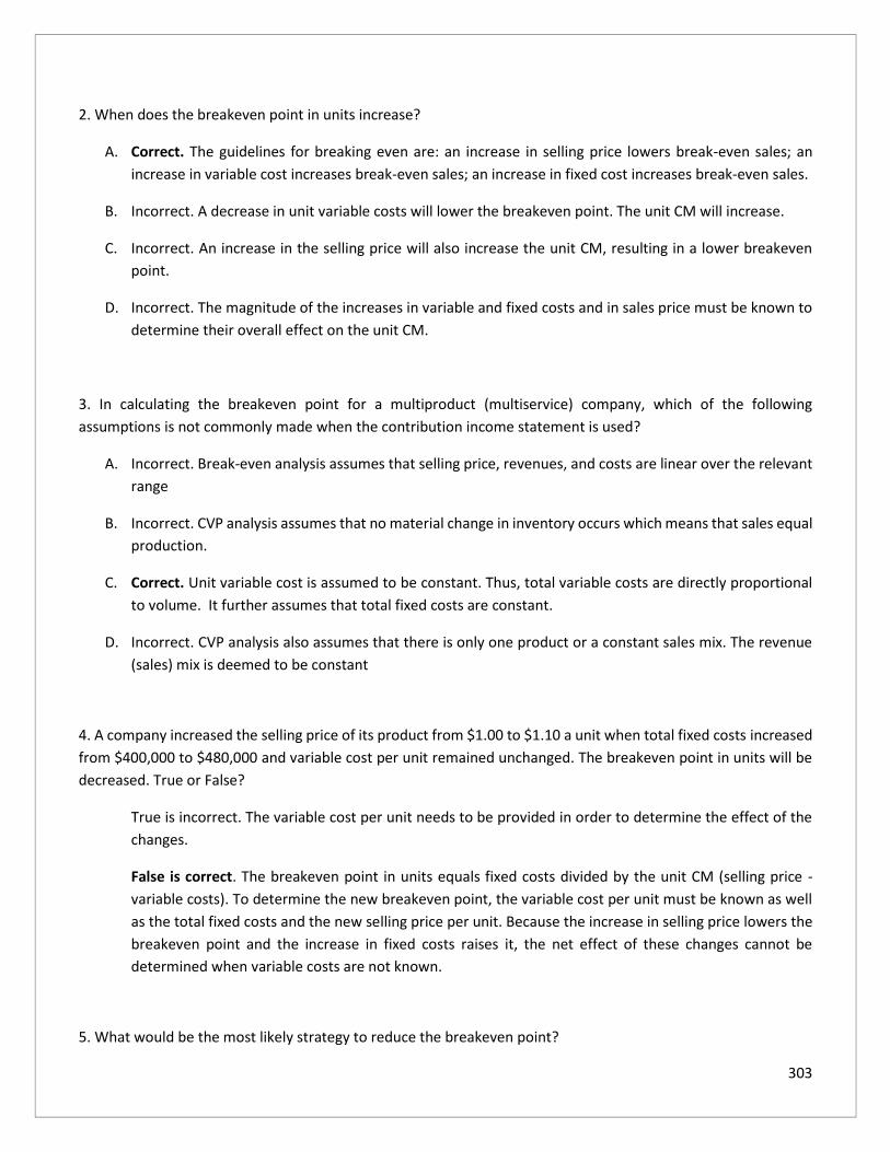
303

2. When does the breakeven point in units increase?

A. Correct. The guidelines for breaking even are: an increase in selling price lowers break-even sales; an

increase in variable cost increases break-even sales; an increase in fixed cost increases break-even sales.

B. Incorrect. A decrease in unit variable costs will lower the breakeven point. The unit CM will increase.

C. Incorrect. An increase in the selling price will also increase the unit CM, resulting in a lower breakeven

point.

D. Incorrect. The magnitude of the increases in variable and fixed costs and in sales price must be known to

determine their overall effect on the unit CM.

3. In calculating the breakeven point for a multiproduct (multiservice) company, which of the following

assumptions is not commonly made when the contribution income statement is used?

A. Incorrect. Break-even analysis assumes that selling price, revenues, and costs are linear over the relevant

range

B. Incorrect. CVP analysis assumes that no material change in inventory occurs which means that sales equal

production.

C. Correct. Unit variable cost is assumed to be constant. Thus, total variable costs are directly proportional

to volume. It further assumes that total fixed costs are constant.

D. Incorrect. CVP analysis also assumes that there is only one product or a constant sales mix. The revenue

(sales) mix is deemed to be constant

4. A company increased the selling price of its product from $1.00 to $1.10 a unit when total fixed costs increased

from $400,000 to $480,000 and variable cost per unit remained unchanged. The breakeven point in units will be

decreased. True or False?

True is incorrect. The variable cost per unit needs to be provided in order to determine the effect of the

changes.

False is correct. The breakeven point in units equals fixed costs divided by the unit CM (selling price -

variable costs). To determine the new breakeven point, the variable cost per unit must be known as well

as the total fixed costs and the new selling price per unit. Because the increase in selling price lowers the

breakeven point and the increase in fixed costs raises it, the net effect of these changes cannot be

determined when variable costs are not known.

5. What would be the most likely strategy to reduce the breakeven point?

304

A. Incorrect. Increasing fixed costs increases the breakeven point. Note that the breakeven point in units

equals fixed costs divided by the unit CM (selling price - variable costs). Fixed costs is in the numerator.

B. Incorrect. Decreasing the contribution margin increases the breakeven point. Note that the contribution

margin is in the denominator in the formula: fixed costs divided by the unit CM (selling price - variable

costs).

C. Correct. The breakeven point in units is equal to the fixed costs divided by the unit CM. The breakeven

point in sales equals the fixed costs divided by the contribution margin ratio. Because fixed costs are in

the numerator and the contribution margin is in the denominator, decreasing the fixed costs and

increasing the contribution margin reduces the breakeven point.

D. Incorrect. Increasing fixed costs and decreasing the contribution margin increases the breakeven point.

Note that the breakeven point in units equals fixed costs divided by the unit CM (selling price - variable

costs).


1. What are ‘relevant costs’?

A. Incorrect. Both fixed and variable costs can be either relevant or irrelevant depending upon the

circumstances. Fixed costs are usually irrelevant to a future decision.

B. Correct. The relevant costs are the future costs that differ between the decision alternatives. Therefore,

the sunk costs are not relevant to these decisions because they are past costs. The incremental or

differential costs are relevant because they are the ones that differ between the alternatives.

C. Incorrect. Relevant costs are expected future costs that differ among decision choices.

D. Incorrect. Past costs are sunk costs. Because they cannot be changed by management action, they are not

relevant.

2. There is a market for both product X and product Y. Which of the following costs and revenues would be most

relevant in deciding whether to sell product X or process it further to make product Y?

A. Incorrect. The cost of making X is a sunk cost (irrelevant). In addition, only X or Y, not both, can be sold.

B. Incorrect. Only the relevant, incremental costs are considered.

C. Correct. Incremental costs are the additional costs incurred for accepting one alternative rather than

another. Questions involving incremental costing (sometimes called differential costing) decisions are

based upon a variable costing analysis. The typical problem for which incremental cost analysis can be

305

used involves two or more alternatives, for example, selling or processing further. The decision will rely

exclusively on additional revenue compared to the additional costs incurred due to further processing.

D. Incorrect. Y is made only after X is completed.


1. The master budget ___________

A. Incorrect. The master budget does not contain actual results.

B. Correct. The master budget is classified broadly into two categories-the operational budget and the

financial budget. The operational budget reflects the results of operating decisions and provides data

needed to prepare a budgeted income statement.

C. Incorrect. The master budget reflects all applicable expected costs, whether or not controllable by

individual managers.

D. Incorrect. The master budget is not structured to allow determination of manufacturing cost variances,

which requires using the flexible budget and actual results.

2. What does the master budget process usually begin with?

A. Correct. The sales budget is the starting point in preparing the master budget since estimated sales

volume influences nearly all other items appearing in the master budget. The sales budget, which

ordinarily indicates the quantity of each product expected to be sold, allows all departments to plan their

needs. Once a firm can estimate sales, the next step is to decide how much to produce or purchase.

B. Incorrect. The production budget normally cannot be prepared until the expected sales are known. The

number of units expected to be manufactured to meet budgeted sales and inventory requirements is set

forth in the production budget.

C. Incorrect. The overhead budget is another term for the budget reflecting the results of operating

decisions. It cannot be prepared until after the sales and production budgets are prepared.

D. Incorrect. Preparation of the cash budget is the last step in the overall budgeting process. The cash budget

is determined after the operating budgets such as the sales and production budgets are prepared.

3. A company had sales last year of $10 million, with net income equal to 6% of sales. This year the sales are

expected to be $11.2 million. The accounts receivable balance was $1.5 million at the end of last year. Using the

percentage-of-sales method, what is the accounts receivable balance at the end of this year forecasted to be?

306

A. Incorrect. $1,572,000 is based on adding the percentage increase in net income to the previous amount

of receivables {[6% x ($11,200,000 - $10,000,000)] + $1,500,000}.

B. Correct. Percentage of sales is the most widely used method for projecting the company's financing needs.

This method involves estimating the various expenses, assets, and liabilities for a future period as a

percent of the sales forecast and then using these percentages, together with the projected sales, to

construct pro forma balance sheets. This method is based on the assumption that most balance sheet

amounts directly correlate with sales and that the current levels of all assets are optimal for the current

sales level. Thus, given that last year's receivables equaled 15% of sales ($1,500,000 ÷ $10,000,000), this

year's ending receivables balance is expected to be $1,680,000 (15% x $11,200,000).

C. Incorrect. $2,172,000 is based on adding profit as a percentage of sales to last year's receivables

[$1,500,000 + (6% x $11,200,000)].

D. Incorrect. $2,700,000 equals past receivables plus the additional sales.

4. Identify the statement below that represents a required underlying assumption for using the percentage-of-

sales technique to develop pro forma financial statements.

A. Incorrect. If economies of scale exist in the use of assets, the ratios of assets to sales are not constant.

B. Correct. This method states balance sheet amounts as percentages of sales and then multiplies future

sales by these percentages to develop pro forma financial statements. Your company is assumed to be

operating at full capacity. Based on this assumption, the firm does not have adequate production capacity

to absorb projected increases in sales and may require an additional investment in assets. Thus, a greater

amount of assets will be required for a greater amount of sales (e.g., receivables and cash requirements

will increase). The asset-to-sales ratios must be constant when applying the percentage-of-sales

forecasting method. If the current levels of assets are considered to be optimal for the current sales level,

that is, if assets are efficiently used, the asset-to-sales ratios are constant.

C. Incorrect. If fixed assets must be added in large, discrete amounts, the ratios are not constant.

D. Incorrect. If ratios vary with economic cycles, the percentage-of-sales method is inappropriate.


1. When preparing a performance report for a cost center using flexible budgeting techniques, what should the

budget cost column be based on?

A. Incorrect. The static (or fixed) budget amount is not useful for comparison purposes. The budget for the

actual activity level achieved is more important. You do not want to compare apples with oranges.

307

B. Incorrect. Prior-year figures are not useful if activity levels are different.

C. Correct. If a report is to be used for performance evaluation, the budget cost column should be based on

the actual level of activity for the period. The ability to adjust amounts for varying activity levels is the

primary advantage of flexible budgeting. Note that flexible budgets are primarily used to accurately

measure performance because they compare actual costs for a given output with the budgeted costs for

the same level of output.

D. Incorrect. A budget based on planned activity level is not as meaningful as one based on actual activity

level. Performance must be measured on an apple by apply basis.

2. A flexible budget is appropriate for ____________

A. Incorrect. Flexible budgets are useful for controlling variable costs, including selling and administrative

costs.

B. Incorrect. A flexible budget is prepared for a specific range of activity.

C. Correct. The flexible budget is geared toward a range of activities rather than a single level of activity. A

flexible budget employs budgeted figures at different capacity levels. This flexibility is important if costs

vary with the activity level. Thus, a flexible budget is particularly appropriate for control of direct labor

and direct materials (both variable costs), but it is not necessary for control of fixed factory overhead. By

definition, fixed overhead costs do not change as activity levels change.

D. Incorrect. Flexible budgets are useful for controlling variable costs, including variable factory overhead

and variable selling and administrative costs.

3. Which one of the following is true concerning standard costs?

A. Incorrect. Standard costs should be attainable under conditions of efficient operation.

B. Incorrect. A standard cost system is ideally suited to a costing system.

C. Correct. Standards are used as a norm against which actual results may be compared. One of the benefits

of a standard cost system is that it can be used to motivate employees to achieve specified goals.

D. Incorrect. All material variances should be investigated, whether favorable or unfavorable.

4. The standard unit cost is used in the calculation of materials price and materials quantity (usage) variances.

True or False?

308

True is correct. The materials price variance is calculated by multiplying the difference between the actual

price and standard price by the actual units purchased. The materials usage variance is calculated by

multiplying the difference between the actual usage and the standard usage by the standard price. Thus,

the standard unit cost is used to compute both the materials price variance and the materials usage

variance.

False is incorrect. Standard price is used in the calculation of both materials price variances and materials

usage variances: Materials Price Variance = (Standard price - Actual price) x Actual quantity; Materials

Quantity Variance = (Standard quantity - Actual quantity) x Standard price.

5. Under a standard cost system, who has responsibility for the materials price variances?

A. Incorrect. The production manager has no control over the price paid for materials.

B. Incorrect. The cost accounting manager has no control over the price paid for materials.

C. Incorrect. The sales manager has no control over the price paid for materials.

D. Correct. The materials price variance is the difference between the standard price and the actual price

paid for materials. This variance is usually the responsibility of the purchasing department. Thus, the

purchasing manager has an incentive to obtain the best price possible.

6. Under a standard cost system, who has responsibility for the materials usage (quantity) variances?

A. Correct. The materials quantity variance is the difference between actual and standard quantities used in

production, times the standard price. An unfavorable materials quantity variance is usually caused by

waste, shrinkage, or theft. Thus, it may be the responsibility of the production department because excess

usage occurs while the materials are in that department. Industrial engineering may also play a role

because it is responsible for the design of the production process.

B. Incorrect. Purchasing is less likely to affect the materials quantity variance.

C. Incorrect. Sales have no effect on the materials quantity variance.

D. Incorrect. The materials quantity variance =(Standard quantity - Actual quantity) x Standard price does

not use sales data.

7. Which of the following could cause an unfavorable direct labor efficiency variance?

A. Incorrect. A variable overhead spending variance may be affected by, but does not affect, the direct labor

efficiency variance. Variable overhead includes indirect, not direct labor.

309

B. Incorrect. Variable overhead includes indirect, not direct, labor. A variable overhead spending variance

does not influence the direct labor efficiency variance.

C. Incorrect. The volume variance is unrelated to the direct labor efficiency variance.

D. Correct. An unfavorable direct labor efficiency variance results when production requires more labor

hours than expected, for example, because employees take longer work breaks than anticipated when

the standards were established. The variance can also be the result of production delays, such as those

caused by poor quality materials or materials shortages. Thus, an unfavorable materials quantity variance

could indicate that excessive materials were used.

8. How is labor rate variance computed?

A. Incorrect. The actual hours must be used to determine the labor rate variance. Price (rate, spending)

variance is calculated as follows: (Standard price - Actual price) x Actual quantity

B. Incorrect. This formula gives no useful variances. Quantity (usage, efficiency) variance is formulated in the

following manner: (Standard quantity - Actual quantity) x Standard price

C. Correct. The labor rate variance is computed by finding the difference between the standard and the

actual rates and then multiplying by actual hours: AH(AR - SR).

D. Incorrect. The difference between standard and actual hours, times the difference between standard and

actual rates, is the rate/usage variance in a three-way analysis of labor variances (not widely used).


1. What is required to determine the appropriate level of working capital for a firm?

A. Incorrect. Management of fixed assets is not a factor in working capital management.

B. Incorrect. Capital structure and dividend policy are factors involved in capital structure finance, not in

working capital financial management.

C. Incorrect. Short-term debt is usually less expensive than long-term debt.

D. Correct. A company must maintain a level of working capital sufficient to pay bills as they come due.

Failure to do so is technical insolvency and can result in involuntary bankruptcy. Unfortunately, holding

current assets for purposes of paying bills is not profitable for a company because they usually offer a low

return compared with longer-term investments. Thus, the skillful management of working capital requires

a balancing of a firm's desire for profit with its need for adequate liquidity.

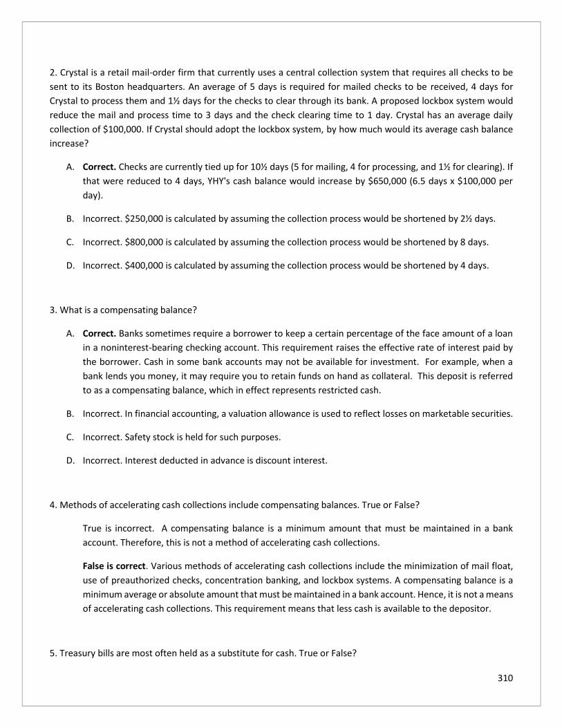
310

2. Crystal is a retail mail-order firm that currently uses a central collection system that requires all checks to be

sent to its Boston headquarters. An average of 5 days is required for mailed checks to be received, 4 days for

Crystal to process them and 1½ days for the checks to clear through its bank. A proposed lockbox system would

reduce the mail and process time to 3 days and the check clearing time to 1 day. Crystal has an average daily

collection of $100,000. If Crystal should adopt the lockbox system, by how much would its average cash balance

increase?

A. Correct. Checks are currently tied up for 10½ days (5 for mailing, 4 for processing, and 1½ for clearing). If

that were reduced to 4 days, YHY's cash balance would increase by $650,000 (6.5 days x $100,000 per

day).

B. Incorrect. $250,000 is calculated by assuming the collection process would be shortened by 2½ days.

C. Incorrect. $800,000 is calculated by assuming the collection process would be shortened by 8 days.

D. Incorrect. $400,000 is calculated by assuming the collection process would be shortened by 4 days.

3. What is a compensating balance?

A. Correct. Banks sometimes require a borrower to keep a certain percentage of the face amount of a loan

in a noninterest-bearing checking account. This requirement raises the effective rate of interest paid by

the borrower. Cash in some bank accounts may not be available for investment. For example, when a

bank lends you money, it may require you to retain funds on hand as collateral. This deposit is referred

to as a compensating balance, which in effect represents restricted cash.

B. Incorrect. In financial accounting, a valuation allowance is used to reflect losses on marketable securities.

C. Incorrect. Safety stock is held for such purposes.

D. Incorrect. Interest deducted in advance is discount interest.

4. Methods of accelerating cash collections include compensating balances. True or False?

True is incorrect. A compensating balance is a minimum amount that must be maintained in a bank

account. Therefore, this is not a method of accelerating cash collections.

False is correct. Various methods of accelerating cash collections include the minimization of mail float,

use of preauthorized checks, concentration banking, and lockbox systems. A compensating balance is a

minimum average or absolute amount that must be maintained in a bank account. Hence, it is not a means

of accelerating cash collections. This requirement means that less cash is available to the depositor.

5. Treasury bills are most often held as a substitute for cash. True or False?

311

True is correct. A treasury bill is a short-term U.S. government obligation that is sold at a discount from

its face value. A treasury bill is highly liquid and nearly risk-free, and it is often held as a substitute for

cash.

False is incorrect. A Treasury bill is almost as safe and liquid as cash.

6. Using a 360-day year, what is the opportunity cost to a buyer of NOT accepting terms 3/10, net 45?

A. Incorrect. 55.67% is based on terms of 3/10, net 30.

B. Correct. Payments should be made within discount periods if the return is more than the firm's cost of

capital. With terms of 3/10, net 45, the buyer is earning a 3% savings for paying on the tenth day, or 35

days earlier than would otherwise be required. For example, on a $1,000 invoice, the payment would be

only $970. The $30 savings is comparable to interest earned on a $970 loan to the vendor (the payment

is not due for another 35 days). The interest rate on this hypothetical loan is 3.09278% ($30/$970). That

return is for a 35-day period. Annualizing the return requires determining the number of 35-day periods

in a year. Multiplying the return for 35 days times the periods in a year results in an annual rate of return

of about 31.81% [3.09278% x (360 days/35 days)].

C. Incorrect. 22.27% is based on an earning period of 50 days.

D. Incorrect. 101.73% is based on a discount of 9%.

7. When a company offers credit terms of 2/10, net 30, the annual interest cost, based on a 360-day year, is 10.3%.

True or False?

True is incorrect. 10.3% is the annual interest cost for credit terms of 1/10, net/45.

False is correct. Assume that the gross amount of an invoice is $1,000. With a 2% discount, the buyer will

pay only $980 on the tenth day. Thus, the seller is forgoing $20 to receive payment 20 days sooner than

would otherwise be required. The 20-day interest rate is .0204 ($20/$980). The number of 20-day periods

in a year is 18 (360/20). If the interest rate is 2.04% for each 20-day period, the annual interest rate

(rounded to the nearest tenth) is 36.7% (18 x 2.04%).


1. When a company analyzes credit applicants and increases the quality of the accounts rejected, what is the

company is attempting to do?

A. Incorrect. Tightening credit will reduce sales.

B. Incorrect. Tightening credit will reduce bad debt losses.

312

C. Incorrect. Most likely, higher quality accounts will mean a shorter average collection period.

D. Correct. Increasing the quality of the accounts rejected means that fewer sales will be made. The company

is therefore not trying to maximize its sales or increase its bad debt losses. The objective is to reduce bad

debt losses and thereby maximize profits.

2. What does an aging of accounts receivable measure?

A. Incorrect. An aging schedule is used for receivables, not liabilities.

B. Incorrect. An aging schedule concerns specific accounts, not averages.

C. Incorrect. An aging schedule focuses on uncollected receivables.

D. Correct. The purpose of an aging of receivables is to classify receivables by due date. Those that are

current (not past due) are listed in one column, those less than 30 days past due in another column, etc.

The amount in each category can then be multiplied by an estimated bad debt percentage that is based

on a company's credit experience and other factors. The theory is that the oldest receivables are the least

likely to be collectible. Aging the receivables and estimating the uncollectible amounts is one method of

arriving at the appropriate balance sheet valuation of the accounts receivable account.

3. What does the average collection period for a firm measure?

A. Correct. The average collection period measures the number of days between the date of sale and the

date of collection. It should be related to a firm's credit terms. For example, a firm that allows terms of

2/15, net 30, should have an average collection period of somewhere between 15 and 30 days.

B. Incorrect. It describes the concept of float.

C. Incorrect. The average collection period includes the total time before a payment is received, including

the periods both before and after the end of the normal credit period.

D. Incorrect. It describes the normal credit period.


1. What is included in the carrying costs associated with inventory management?

A. Incorrect. Shipping costs are ordering costs, not carrying costs.

B. Correct. Carrying costs include storage costs, insurance costs, interest on capital invested, and

obsolescence.

313

C. Incorrect. It states various ordering (or manufacturing) costs.

D. Incorrect. The set-up costs for a production run are equivalent to ordering costs. Additionally, purchasing

costs are considered costs of ordering.

2. What is included in the ordering costs associated with inventory management?

A. Incorrect. Insurance costs and obsolescence are carrying costs.

B. Incorrect. Obsolescence and storage costs are carrying costs.

C. Correct. Ordering costs are costs incurred when placing and receiving orders. Ordering costs include

purchasing costs, shipping costs, clerical costs, setup costs for a production run, and quantity discounts

lost.

D. Incorrect. Obsolescence and capital invested are carrying costs.

3. Which of the following is an example of a carrying cost?

A. Incorrect. Disruption of production schedules may result from a stockout.

B. Incorrect. Quantity discounts lost are related to ordering costs or inventory acquisition costs.

C. Incorrect. Shipping and handling costs are included in acquisition costs.

D. Correct. Inventory costs fall into three categories: order or setup costs, carrying (holding) costs, and

stockout costs. Carrying costs include storage costs for inventory items plus opportunity cost (i.e., the cost

incurred by investing in inventory rather than making an income-earning investment). Examples are

insurance, spoilage, interest on invested capital, obsolescence, and warehousing costs.

4. In inventory management, which of the following will cause the safety stock to increase?

A. Incorrect. An increase in inventory carrying costs makes it less economical to carry safety stocks. Thus,

safety stocks will be reduced.

B. Incorrect. If the cost of stockouts declines, the incentive to carry large safety stocks is reduced.

C. Correct. A company maintains safety stocks to protect itself against the losses caused by inventory stock-

outs. These can take the form of lost sales or lost production time. Safety stock is necessary because of

the variability in lead time and usage rates. As the variability in lead time increases, a company will tend

to carry larger safety stocks.

314

D. Incorrect. A decline in the variability of usage makes it easier to plan orders, and safety stocks will be less

necessary.

5. What does the economic order quantity formula indicate?

A. Incorrect. The annual quantity of inventory demanded is an input into the formula, not the result.

B. Incorrect. Annual usage is a determinant of annual demand, which is an input into the formula.

C. Incorrect. Safety stock is not reflected in the basic EOQ formula.

D. Correct. The EOQ model is a deterministic model that calculates the ideal order (or production lot)

quantity given specified demand, ordering or setup costs, and carrying costs. The model minimizes the

sum of inventory carrying costs and either ordering or production setup costs.


1. John Watson's uncle recently passed away and included in the property that John inherited is a bond that pays

an 8% coupon, has a face value of $1,000, has 10 years to maturity, and the investors require a rate of return of

10%. Assuming annual coupon payments, what is the value of the bond?

A. Incorrect. $386 results from only taking into account the present value of the lump sum principal of the

bond.

B. Incorrect. $491.60 results from only taking into account the annuity of coupon payments.

C. Incorrect. $614.50 results from incorrectly multiplying the bond's $1,000 face value by the annuity interest

factor, 6.145, instead of the interest factor for the present value of the lump sum, 0.386.

D. Correct. The value of the bond is equal to the sum of (1) the product of the coupon payments and the

correct annuity factor, and (2) the product of the face value of the bond and the correct present value

factor. Because the bond has 10 periods to maturity and the effective interest rate is 10%, the interest

factor for the present value of the lump sum is 0.386, and the interest factor for the present value of the

annuity is 6.145. Therefore, multiplying the $80 annual interest payment by its interest factor of 6.145

equals a present value of $491.60. Also, the present value of the lump sum is equal to the $1,000 face

value of the bond multiplied by 0.386, which equals $386.00. Thus, the total value of the bond is the sum

of these two present values, or $877.60.

2. On November 1, 20X5, a company purchased a new machine that it does not have to pay for until November 1,

20X7. The total payment on November 1, 20X7 will include both principal and interest. Assuming interest at a 10%

rate, the cost of the machine would be the total payment multiplied by what time value of money concept?

315

A. Incorrect. The present value of an annuity determines the value today of a series of future payments (not

merely one payment).

B. Correct. The cost of the machine to the company on November 1, 20X5 is the present value of the

payment to be made on November 1, 20X7. To obtain the present value, i.e., today's price, the future

payment is multiplied by the present value of $1 for two periods at 10%.

C. Incorrect. The future value of an annuity determines the amount available at a specified time in the future

after a series of deposits (investments).

D. Incorrect. The future value of a dollar determines how much will be available at a specified time in the

future based on the single investment (deposit) today.

3. Pole Co. is investing in a machine with a 3-year life. The machine is expected to reduce annual cash operating

costs by $30,000 in each of the first 2 years and by $20,000 in year 3. Using a 14% cost of capital (discount rate),

what is the present value of these future savings? Note: The Present Values of $1 at 14% for period 1 = 0.88, for

period 2 = 0.77, and for period 3 = 0.68. The Present Values of an Annuity of $1 at 14% for period 1 = 0.88, for

period 2 = 1.65, and period 3 = 2.32. )

A. Incorrect. $59,600 equals the present value of a 3-year annuity for $30,000, minus $10,000.

B. Incorrect. The present value of a 3-year annuity of $30,000 is $69,600.

C. Correct. Using a 14% cost of capital and ignoring tax effects, the present value of a $30,000 annuity

discounted over a 2-year period is $49,500 ($30,000 x 1.65). The present value of $20,000 in year 3 is

$13,600 ($20,000 x 0.68). Hence, the total present value of the future savings is $63,100.

D. Incorrect. $69,500 equals the present value of a 2-year annuity for $30,000, plus $20,000.


1. Doro Co. is considering the purchase of a $100,000 machine that is expected to result in a decrease of $25,000

per year in cash expenses after taxes. This machine, which has no residual value, has an estimated useful life of

10 years and will be depreciated on a straight-line basis. For this machine, what would the accounting rate of

return (ARR) based on initial investment be?

A. Incorrect. 10% is the depreciation rate per year.

B. Correct. The ARR is based on the accrual method and does not discount future cash flows. Accordingly,

the ARR equals the decrease in annual cash expenses after taxes minus annual depreciation, divided by

the initial investment. Annual straight-line depreciation is $10,000 [($100,000 cost - $0 salvage value) ÷

10 years]. So the ARR would be ($25,000- $10,000) / $100,000 = 15%.

316

C. Incorrect. Depreciation must be deducted from the $25,000 of cash expenses.

D. Incorrect. Depreciation must be deducted from, not added to, the $25,000 of cash expenses.

2. Neu Co. is considering the purchase of an investment that has a positive net present value (NPV) based on Neu's

12% hurdle rate (minimum required rate of return). What would the internal rate of return be?

A. Incorrect. The IRR of 0 less than the 12% hurdle rate indicates that the NPV should be significantly

negative.

B. Incorrect. The NPV should be 0 when the IRR is equal to the hurdle rate of 12%.

C. Correct. Internal rate of return (IRR) is defined as the rate of interest that equates initial investment (I)

with the PV of future cash inflows. In other words, at IRR, I = PV or NPV = 0. As long as r is greater than

the NPV's hurdle rate, the NPV must be positive (greater than zero). Because Neu has a positive NPV based

on 12%, the IRR must be greater than 12%.

D. Incorrect. The NPV>0 means that the IRR should be greater than the minimum rate of return (12% in this

problem).


1. Which combination of changes in asset turnover and profit margin on sales will maximize the return on

investment?

A. Incorrect. A decrease in margin lowers the return on investment.

B. Correct. Asset turnover measures how efficiently assets are used to produce revenues by dividing sales

by the average total assets. The profit margin measures the net income produced by each dollar of

revenues. As assets are used more efficiently and as each dollar of revenues produces more income, the

return on investment is maximized.

C. Incorrect. As assets are used less efficiently, the return on investment decreases.

D. Incorrect. As assets are used less efficiently and as the profit margin on sales decreases, the return on

investment decreases.

2. Return on investment (ROI) may be calculated by dividing net profit after taxes by debt ratios. True or False?

True is incorrect. ROI cannot be determined using this ratio. A debt ratio is debt divided by total assets.

317

False is correct. The rate of return measures the ability of the company to earn a profit on its total assets.

The formula is: ROI = (net profit after taxes) / (total assets)

3. Return on investment (ROI) may be calculated by multiplying net profit margin by equity. True or False?

True is incorrect. The Du Pont formula (net profit margin times total asset turnover) shows how important

both margin and turnover are in enhancing return on investment (ROI).

False is correct. The Du Pont formula breaks down the return on investment (ROI) into net profit margin and

total asset turnover, as such: ROI = (net profit after taxes) / (total assets) =[(net profit after taxes) / Sales] x

[Sales / (total assets)] = net profit margin x total asset turnover.

4. An investor has been given several financial ratios for a firm but none of the financial reports. Which

combination of ratios can be used to derive return on equity?

A. Incorrect. The market-to-carrying-amount ratio and the total-debt-to-total-assets ratio do not provide any

information about net profit available to shareholders.

B. Correct. The net profit margin equals the net profit available to common shareholders divided by sales.

The total assets turnover equals sales divided by total assets, and the product of these two ratios is the

return on investment (ROI). This result is the basic Du Pont formula. In the extended Du Pont equation,

the ROI is multiplied by the leverage factor, also called the equity multiplier (total assets/common equity).

The extended Du Pont equation gives the return on common equity. This result is obtained because the

total assets and sales factors cancel in the multiplication of the three ratios. ROE = (net profit after taxes)

/ (stockholders’ equity) = [(net profit after taxes) / (total assets)] x [(total assets) / (stockholders’ equity)]

= ROI x Equity Multiplier = net profit margin x total asset turnover x equity multiplier.

C. Incorrect. The price-to-earnings ratio, EPS, and the net profit margin do not provide information about

the carrying amount of common equity.

D. Incorrect. The price-to-earnings ratio and the return-on-assets ratio do not provide information about the

carrying amount of common equity.

5. The following ratios relate to a company’s financial situation compared with that of its industry: The company

has an ROI = 7.9% and an ROE = 15.2%. The industry has an ROI = 9.2% and an ROE = 12.9%. What conclusion

could a financial analyst validly draw from these ratios?

A. Incorrect. The question gave no information about market share.

B. Correct. The use of financial leverage has a multiplier effect on the return on assets. The extended Du

Pont formula illustrates this point by showing that the return on equity equals the ROI times the leverage

318

factory, also called the equity multiplier (total assets/common equity). Thus, greater use of debt increases

the equity multiplier and the return on equity. In this example, the equity multiplier is 1.92 (15.2%

ROE/7.9% ROI), and the industry average is 1.40 (12.9% ROE/9.2% ROI). The higher equity multiplier

indicates that the company uses more debt than the industry average.

C. Incorrect. This comparison is with an industry average, not over time.

D. Incorrect. Share valuation is a response to many factors. The higher-than-average return on equity does

not mean that the company has a more favorable market-to-carrying-amount ratio.


1. What is a successful responsibility accounting reporting system dependent upon?

A. Incorrect. Fixed costs may also be controllable, and some costs not controllable may need to be assigned.

B. Incorrect. Knowledge about the incurrence of a cost rather than controllability may in practice be an

appropriate basis for delegation of responsibility.

C. Correct. Managerial performance should ideally be evaluated only on the basis of those factors

controllable by the manager. Managers may control revenues, costs, and/or investments in resources.

D. Incorrect. Fixed costs can be controllable.

2. When is a segment of an organization an investment center?

A. Incorrect. A profit center is responsible for controlling expenses and generating revenues.

B. Correct. In investment centers, managers are responsible for all activities, including costs, revenues, and

investments. An investment center is a profit center with significant control over the amount of capital

invested. This control extends to investments such as receivables and property, plant, and equipment, as

well as entry into new markets.

C. Incorrect. A cost center has authority only over the sources of supply.

D. Incorrect. A revenue center is responsible for developing markets and selling the firm's products.

3. Responsibility accounting defines an operating center that is responsible for revenue and costs as a(n) _____

A. Incorrect. A revenue center is responsible only for revenues, not costs.

319

B. Correct. A profit center is responsible for both revenues and costs, whereas a cost center is responsible

only for costs.

C. Incorrect. A division can be any type of responsibility center.

D. Incorrect. An operating unit can be organized as any type of center.

4. What is the residual income of an investment center?

A. Incorrect. The residual income equals divisional operating income less minimum return times total

operating assets.

B. Correct. Residual income is the excess of the return on an investment over a targeted amount equal to a

minimum required return on invested capital. The rate used is ordinarily the weighted-average cost of

capital. Thus, an investment center's residual income is the center's income minus the minimum required

return on its invested capital.

C. Incorrect. Residual income is the excess income, not contribution margin, over the minimum required

return.

D. Incorrect. Imputed interest is subtracted from income, not contribution margin. Contribution margin is

sales revenue minus variable costs.

5. Why is residual income (RI) a better measure for performance evaluation of an investment center manager than

return on investment (ROI)?

A. Incorrect. The methods use the same asset base.

B. Incorrect. Both approaches can use the gross book value of assets or any other measure for that matter.

C. Correct. Residual income is the excess of the amount of the ROI over a targeted amount equal to an

imputed interest charge on investment capital. The advantage of using residual income rather than

percentage ROI is that the former emphasizes maximizing a dollar amount instead of a percentage.

Managers of divisions with a high ROI are encouraged to accept projects with returns exceeding the cost

of capital even if those projects reduce the department’s ROI.

D. Incorrect. The use of the residual income method requires knowledge of the cost of capital; thus

arguments about the implicit cost of interest may escalate with use of the residual income method.

6. Residual income is a performance evaluation that is used in conjunction with, or instead of, return on

investment (ROI In many cases, why is residual income preferred to ROI?

320

A. Incorrect. Both measures represent the results for a single period.

B. Correct. Residual income equals earnings in excess of a minimum desired return. Thus, it is measured in

dollars. If performance is evaluated using ROI, a manager may reject a project that exceeds the minimum

return if the project will decrease overall ROI. For example, given a target rate of 20%, a project with an

ROI of 22% might be rejected if the current ROI is 25%.

C. Incorrect. The target rate for ROI is the same as the imputed interest rate used in the residual income

calculation.

D. Incorrect. The same investment base should be employed in both methods. The investment base must

be measured consistently: average investment or year-end investment. If the data is available, average

investment should be used.

7. The price that one division of a company charges another division for goods or services provided is called

negotiated pricing. True or False?

True is incorrect. There are several different approaches to determine a transfer price. Negotiated pricing

is an approach, along with the variable cost-based price and the market price.

False is correct. A transfer price is the price charged by one segment of an organization for a product or

service supplied to another segment of the same organization.

8. What is a limitation of transfer prices based on actual cost?

A. Incorrect. Inefficiencies are charged to the buying department. The transfer should be at standard variable

cost so as to isolate any variance resulting from the buyer.

B. Correct. The optimal transfer price of a selling division should be set at a point that will have the most

desirable economic effect on the firm as a whole while at the same time continuing to motivate the

management of every division to perform efficiently. Setting the transfer price based on actual costs

rather than standard costs would give the selling division little incentive to control costs (pass cost

efficiencies).

C. Incorrect. By definition, cost-based transfer prices are not adjusted by some markup.

D. Incorrect. Cost-based transfer prices provide the advantages of clarity and administrative convenience.

321


1. Which one of the following financial instruments generally provides the largest source of short-term credit for

small firms?

A. Incorrect. Installment loans are usually a longer-term source of financing and are more difficult to acquire

than short-term sources of financing.

B. Incorrect. Commercial paper is normally used only by large companies with high credit ratings.

C. Correct. Trade credit (accounts payable) refers to balances owed to suppliers. It is a spontaneous

(recurring) financing source, since it comes from normal operations, and is the least expensive form of

financing inventory. Because of its ease in use, trade credit is the largest source of short-term financing

for many firms both large and small.

D. Incorrect. Bankers' acceptances are drafts drawn on bank deposits; the acceptance is a guarantee of

payment at maturity. It is a popular source of short-term financing, albeit not the largest source.

2. If a firm borrows $500,000 at 10% and is required to maintain $50,000 as a minimum compensating balance at

the bank, what is the effective interest rate on the loan?

A. Incorrect. 10% is the nominal rate.

B. Correct. At 10%, the interest on a $500,000 loan is $50,000 per year. However, the $500,000 loan is

effectively reduced to $450,000 of usable funds by the compensating balance requirement. Thus, the

borrower pays $50,000 of interest for a $450,000 loan, an effective rate of 11.1% ($50,000/$450,000).

C. Incorrect. 9.1% equals $50,000 divided by $550,000.

D. Incorrect. 12.2% equals $55,000 divided by $450,000.

3. What is an example of secured short-term financing?

A. Incorrect. Commercial paper is a type of unsecured, short-term promissory note issued by large firms to

other firms, insurance companies, mutual funds, etc.

B. Correct. A document of title is usually issued by a bailee covering goods in the bailee's possession or care

(UCC 1-201). It represents ownership of the goods and is ordinarily needed to obtain the goods from the

bailee. The two major types of documents of title are bills of lading (issued by carriers) and warehouse

receipts. With a warehouse receipt, the lender receives an interest in the inventory stored at a public

warehouse; however, the fixed costs of this arrangement are high. There may be a field warehouse

arrangement in which the warehouse sets up a secured area directly at your location. You have access to

the goods but must continually account for them.

322

C. Incorrect. A revolving credit agreement is a formal line of credit, usually with a bank, that large firms often

use.

D. Incorrect. A line of credit is an arrangement, which may be formal or informal, between a commercial

bank and its customer concerning the maximum loan amount available.

4. How would a small retail business most likely finance its merchandise inventory?

A. Incorrect. Only large companies with excellent credit ratings have access to the commercial paper market.

B. Incorrect. A retail store must have instant access to its inventory to provide continuous services to

customers. Thus, a loan on a warehouse receipt loan would not be suitable because the inventory would

not be in the immediate possession of the seller.

C. Correct. A small retail store would not have access to major capital markets. In fact, the only options

available, outside of owner financing, are bank loans and a line of credit from suppliers. It is this latter

alternative that is most often used because it permits the store to finance inventories for 30 to 60 days

without incurring interest costs. A line of credit is an arrangement between a bank and a borrower in

which the bank commits itself to lend up to a certain maximum amount to the borrower in a given period.

D. Incorrect. A chattel mortgage is most often used for financing moveable equipment. It is not well-suited

to financing inventory of a small retailer with high turnover because of the difficulty of identification.

5. A manufacturing firm wants to obtain a short-term loan and has approached several lending institutions. All of

the potential lenders are offering the same nominal interest rate but the terms of the loans vary. Which of the

following combinations of loan terms will be most attractive for the borrowing firm?

A. Correct. The most desirable set of terms are those that result in the lowest cost of borrowing. Discount

interest results in a higher effective borrowing cost than simple interest because the bank deducts interest

in advance so the borrower receives less than the face value of the loan. A compensating balance results

in a higher effective borrowing cost because the compensating balance is an amount of cash that the firm

is unable to use. The cheapest terms, given that all options have the same nominal interest rate, will be

simple interest with no compensating balance.

B. Incorrect. Discount interest results in a higher effective borrowing cost than simple interest because the

bank deducts interest in advance so the borrower receives less than the face value of the loan.

C. Incorrect. A compensating balance results in a higher effective borrowing cost because the compensating

balance is an amount of cash that the firm is unable to use.

D. Incorrect. Discount interest and a compensating balance are disadvantageous to the borrower.

323


1. What is a major difference between operating and financial leases?

A. Incorrect. Operating leases usually provide for maintenance, but financial leases do not.

B. Incorrect. Operating lease contracts are written for a period less than the economic life.

C. Correct. Operating leases provide both financing and maintenance services to the lessee. An operating or

service lease is usually for a term less than the economic life of the asset, and the lease payments are for

an amount less than the full cost. Moreover, a cancellation clause in the agreement usually permits the

lessee to return the asset before expiration of the term, for example, because of technological change. A

financial lease is tantamount to a sale financed by the lessor. The payments are equal to the full cost of

the asset, cancellation is not permitted, and maintenance is ordinarily not provided.

D. Incorrect. The lessor finances the assets leased for an operating lease.


1. How do preferred and common stock differ?

A. Incorrect. Failure to pay dividends will not force the firm into bankruptcy, whether the dividends are for

common or preferred stock. Only failure to pay interest will force the firm into bankruptcy.

B. Incorrect. Preferred dividends are fixed.

C. Correct. In the event of bankruptcy, the claims of preferred shareholders must be satisfied before

common shareholders receive anything. The interests of common shareholders are secondary to those of

all other claimants.

D. Incorrect. Neither common nor preferred dividends are tax-deductible.

2. Which one of the following statements correctly compares bond financing alternatives?

A. Incorrect. Callable bonds sometimes pay a slightly higher rate of interest. Investors may demand a greater

return because of the uncertainty over the true maturity date.

B. Incorrect. Conversion is at the option of the investor.

C. Correct. A callable bond can be recalled by the issuer prior to maturity. A call provision is detrimental to

the investor because the issuer can recall the bond when market interest rates decline. It is usually

exercised only when a company wishes to refinance high-interest debt.

324

D. Incorrect. A sinking fund provision requires an issuer to retire a certain portion of its bonds each year or

set aside money for repayment in the future. Such a provision increases the probability of repayment for

bondholders but does not prohibit early redemption.

3. What are debentures?

A. Incorrect. Unlike, debentures must pay interest regardless of earnings levels.

B. Incorrect. Debentures are not subordinated except to the extent of assets mortgaged against other bond

issues. Debentures are a general obligation of the borrower and rank equally with convertible bonds.

C. Correct. Debentures are unsecured bonds. Although no assets are mortgaged as security for the bonds,

debentures are secured by the full faith and credit of the issuing firm. Debentures are a general obligation

of the borrower. Only companies with the best credit ratings can issue debentures because only the

company's credit rating and reputation secure the bonds.

D. Incorrect. Debentures are not secured by mortgages on specific assets.

4. Zero-coupon bonds issued by corporations _______________

A. Incorrect. These bonds are sold at a discount.

B. Incorrect. These bonds are sold at a discount, not at a premium.

C. Incorrect. These bonds are subject to taxes.

D. Correct. Zero-coupon bonds pay no interest but sell at a deep discount from their face value. A relatively

new type of bond, these instruments are very useful to both investors and investees. The need to reinvest

the interest on normal coupon bonds renders the final return uncertain because future reinvestment rates

are uncertain. With zero-coupon bonds, the investor knows exactly the return (s)he will earn. Investors

might, therefore, be willing to pay a premium for them, which in turn might lead firms to issue them. No

interest payments means the firm faces no additional insolvency risk from the issue until it matures.

5. What are junk bonds?

A. Correct. Junk bonds are high risk and therefore high-yield securities that are normally issued when the

debt ratio is very high. Thus, the bondholders have as much risk as the holders of equity securities. Such

bonds are not highly rated by credit evaluation companies. Junk bonds have become accepted because of

the tax-deductibility of the interest paid.

B. Incorrect. Junk bonds are not yet worthless; they simply bear high-interest rates and high risk.

325

C. Incorrect. Junk bonds typically offer high yields.

D. Incorrect. Junk bonds are not ones that have been downgraded; they were never high grade.

6. The characteristics of venture capital include all of the following EXCEPT:

A. Incorrect. Venture capital investments are typically private placements.

B. Correct. The concept of venture (risk) capital applies to new enterprises that might not be able to obtain

funds in the usual capital markets because of the riskiness of new products. Such companies sometimes

try to place securities, normally common stock, with venture capital firms. These are normally private

placements of the securities and thus not subject to SEC regulation. The venture capitalists risk low

liquidity for their investments until the young corporation becomes successful. The payoff may be

substantial if the company does succeed. There is no minimum holding period for venture capital

investments.

C. Incorrect. Common stock is usually a part of most venture capital deals. Venture capitalists want large

payoffs in exchange for the risk assumed.

D. Incorrect. Venture capital investments typically are not liquid for a substantial time after the investment

is made.


1. The basic financial statements include a balance sheet, income statement, and statement of activities. True or

False?

True is incorrect. The basic statements are the balance sheet, income statement, and statement of cash

flows.

False is correct. Under GAAP, the basic required statements are the balance sheet, income statement,

and statement of cash flows. A statement of cash flows is now a required part of a full set of financial

statements of all business entities (both publicly held and privately held).

2. What is the primary purpose of the balance sheet?

A. Incorrect. The measurement attributes of assets include but are not limited to fair value.

B. Incorrect. Financial statements reflect the going concern assumption. Hence, they usually do not report

forced liquidation values.

326

C. Correct. The balance sheet presents three major financial accounting elements: assets, liabilities, and

equity. Assets are probable future economic benefits resulting from past transactions or events. Liabilities

are probable future sacrifices of economic benefits arising from present obligations as a result of past

transactions or events. Equity is the residual interest in the assets after deduction of liabilities.

D. Incorrect. The future value of a company’s stock is more dependent upon future operations and investors’

expectations than on the data found in the balance sheet.

3. A financial statement includes all of the following items: operating activities, financial activities, and investing

activities. What financial statement is this?

A. Correct. A statement of cash flows is a required financial statement. Its primary purpose is to provide

information about cash receipts and payments by reporting the cash effects of an enterprise’s operating,

investing, and financing activities. Because the statement or a separate schedule reconciles net income

and net operating cash flow, depreciation, a noncash expense, is included in the presentation.

B. Incorrect. The balance sheet does not include periodic net income or depreciation expense.

C. Incorrect. The income statement does not have captions for operating and financing activities.

D. Incorrect. Retained earnings does not include captions for operating and investing activities, depreciation,

and net income.


1. What does the term "double-entry system" refer to?

A. Incorrect. The distinction between real and nominal accounts is based on the relative permanence of

accounts rather than the double entry, self-balancing attribute of accounting systems.

B. Correct. In the double-entry system, each transaction is composed of two parts, debits and credits. The

debits must equal the credits, and the sum of all debits for all transactions in a double-entry system must

equal the sum of all credits.

C. Incorrect. Many journals may be used, e.g., general journal, sales journal, cash receipts journal, and cash

payments journal.

D. Incorrect. Even though journals and ledgers are parts of all double entry systems, they have nothing to do

with the term "double entry."

2. What is a chart of accounts?

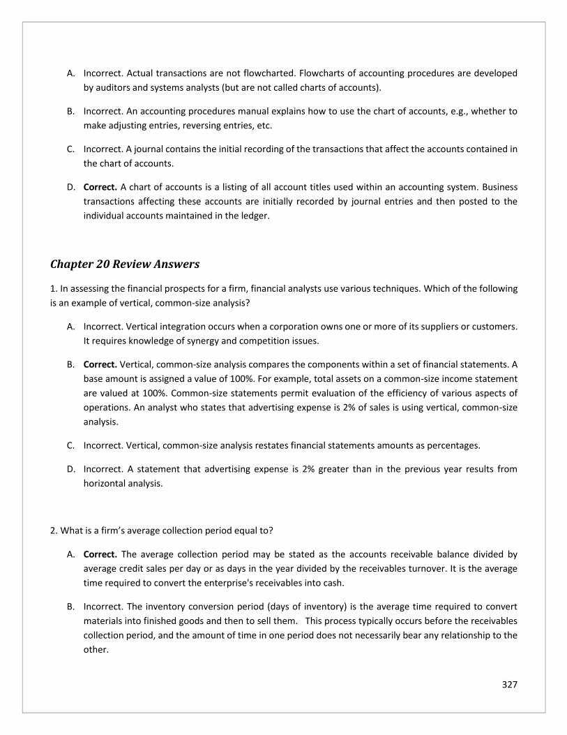
327

A. Incorrect. Actual transactions are not flowcharted. Flowcharts of accounting procedures are developed

by auditors and systems analysts (but are not called charts of accounts).

B. Incorrect. An accounting procedures manual explains how to use the chart of accounts, e.g., whether to

make adjusting entries, reversing entries, etc.

C. Incorrect. A journal contains the initial recording of the transactions that affect the accounts contained in

the chart of accounts.

D. Correct. A chart of accounts is a listing of all account titles used within an accounting system. Business

transactions affecting these accounts are initially recorded by journal entries and then posted to the

individual accounts maintained in the ledger.


1. In assessing the financial prospects for a firm, financial analysts use various techniques. Which of the following

is an example of vertical, common-size analysis?

A. Incorrect. Vertical integration occurs when a corporation owns one or more of its suppliers or customers.

It requires knowledge of synergy and competition issues.

B. Correct. Vertical, common-size analysis compares the components within a set of financial statements. A

base amount is assigned a value of 100%. For example, total assets on a common-size income statement

are valued at 100%. Common-size statements permit evaluation of the efficiency of various aspects of

operations. An analyst who states that advertising expense is 2% of sales is using vertical, common-size

analysis.

C. Incorrect. Vertical, common-size analysis restates financial statements amounts as percentages.

D. Incorrect. A statement that advertising expense is 2% greater than in the previous year results from

horizontal analysis.

2. What is a firm’s average collection period equal to?

A. Correct. The average collection period may be stated as the accounts receivable balance divided by

average credit sales per day or as days in the year divided by the receivables turnover. It is the average

time required to convert the enterprise's receivables into cash.

B. Incorrect. The inventory conversion period (days of inventory) is the average time required to convert

materials into finished goods and then to sell them. This process typically occurs before the receivables

collection period, and the amount of time in one period does not necessarily bear any relationship to the

other.

328

C. Incorrect. The cash conversion cycle equals the inventory conversion period, plus the receivables

collection period, minus the payables deferral period (average time between resource purchases and

payment of cash for them). It estimates the time between when the enterprise makes payments and when

it receives cash inflows.

D. Incorrect. The inventory divided by the sales per day is the inventory conversion period (days of

inventory).

3. What type of ratio is the profit margin ratio?

A. Incorrect. Activity ratios measure management’s efficiency in using specific resources.

B. Correct. Profit margin is a profitability ratio. Profit margin = (net income) / (net sales).

C. Incorrect. Liquidity ratios indicate the ability of a company to meet short-term obligations.

D. Incorrect. Leverage or equity ratios concern the relationship of debt to equity and measure the impact of

the debt on profitability and risk.

4. What is the times-interest-earned ratio primarily an indication of?

A. Incorrect. Liquidity ratios, e.g., the current ratio, indicate the relationship of current assets to current

liabilities.

B. Incorrect. Asset management ratios indicate how effectively the enterprise is using its assets.

C. Correct. The times-interest-earned ratio equals (Income from operations) / (Interest Expense). It

measures the extent to which operating profit can decline before the enterprise is unable to meet its

annual interest cost. Thus, it is a measure of debt-paying capacity (solvency).

D. Incorrect. Profitability ratios measure operating results.

5. A company has 100,000 outstanding common shares with a market value of 20 per share. Dividends of 2 per

share were paid in the current year, and the enterprise has a dividend-payout ratio of 40%. What is the price-to-

earnings ratio of the company?

A. Incorrect. 2.5 equals EPS divided-by dividends per share.

B. Incorrect. 10 equals share price divided by dividends per share.

329

C. Correct. The P-E ratio equals the share price divided by EPS. If the dividends per share equaled 2 and the

dividend-payout ratio was 40%, EPS must have been 5 (2/0.4). Accordingly, the P-E ratio is 4 (20 share

price/5 EPS).

D. Incorrect. 50 equals price per share divided by the dividend-payout percentage.

6. Horn Company paid out one-half of last year's earnings in dividends. Horn’s earnings increased by 20%, and the

amount of its dividends increased by 15% in the current year. What was Horn's dividend payout ratio for the

current year?

A. Incorrect. 50% is the prior-year payout ratio.

B. Incorrect. 57.5% is 115% of the prior-year payout ratio.

C. Correct. The prior-year dividend payout ratio was 50%. Hence, if prior-year net income was X, the total

dividend payout would have been 50%X. If earnings increase by 20%, current year income will be 120%X.

If dividends increase by 15%, the total dividends paid out will be 57.5%X (115% x 50%X), and the new

dividend payout ratio will be 47.9% (57.5%X ÷ 120%X).

D. Incorrect. 78% equals 65% of 120%.

7. Financial ratio analysis has no limitation when it comes to comparing financial fitness among firms. True or

False?

True is incorrect. Ratio analysis provides useful information regarding the efficiency of operations and the

stability of financial condition. Nevertheless, it has several inherent limitations, such as firms using

different accounting and operating policies, multiple lines of businesses, and different sources of

information. Each of these factors impairs the comparability of financial statement amounts and the ratios

derived from them.

False is correct. Financial ratios, for example, calculated based on different sources of information, can

lead to misleading interpretations.

for managers and entrepreneurs

Documents