for the p-50 industrial robot by

A Microprocessor Based Development System

for the

P-50 Industrial Robot

by

R. Rajkumar

Thesis submitted to the Faculty of the

Virginia Polytechnic Institute and State University

in partial fulfillment of the requirements for the degree of

Master of Science

in

Electrical Engineering

APPROVED:

Dr. Charles E. Nunnally

Dr. S. Wahid Zewari Dr. Paul M. Lapsa

June, 1985

Blacksburg, Virginia

A Microprocessor Based Development System

for the

P-50 Industrial Robot

by

R. Rajkumar

Dr. Charles E. Nunnally

Electrical Engineering

(ABSTRACT)

With the current interest in the control of robots, the

need for an industrial robot as a research tool has become

preeminent. This thesis presents the concepts and the design

for a microprocessor based development system for the P-50

Process Robot, in an effort to convert it into a Robot Con-

trol Development System.

Various control philosophies were reviewed to arrive at a

hierarchical control structure that provides maximum flexi-

bility and control over every degree of freedom of the robot

arm.

The working of the original controller of the P-50 robot

was studied in detail to facilitate design of interface cir-

cuits that transfer control of the arm to the augmented con-

troller. All the hardware required for the controller was

designed and tested. Guidelines for developing the software

as well as schematics for constructing the remaining hardware

circuits, are provided.

The conclusion discusses modifications that could be made

to this design and instructions for using the fully developed

controller.

iv

ACKNOWLEDGEMENTS

I thank Dr. Wahid Zewari, who conceived this project, for

his tremendous interest and support, for teaching me the

basics of robot kinematics &: control and for boosting my

morale at times, when everything seemed to go wrong.

Dr. Charles Nunnally not only guided me through the prep-

aration of this thesis, but also gave advice on the se-

lection of hardware for developing the system. I am thankful

to him for all the help and support he provided.

I would like to thank Dr. Paul Lapsa for serving on my

graduate committee.

The design of the servo for the development system would

never have been completed without the help from Doug Hopkins·,

in understanding the working of the original P-50 controller.

I also thank many others who made this work possible: Mark

Hopkins shared his experiences in designing a controller for

the Rhino robot;

immensely with

Frank Caldwell and Billy Shepherd helped

much-needed electronic components; Bob

Lineberry provided help with the design of some of the cir-

cuits; Greg Sherman, who could be called an 'IBM PC expert',

wrote programs for the user interface level of the control-

ler; Ashit Gandhi and Jayaram Sankar calculated the mechan-

ical parameters of the manipulator arm and simulated it using

the Interactive Simulation Language.

Acknowledgements V

TAB LE OF CONTENTS

1.0 Introduction. . . . . . . . . . . . . . 1

1.1 Classification of Robots. 1

1.2 System Requirements. 3

1. 3 The Control Structure. . . . 4

1.4 System Overview. 6

2.0 Kinematics, Trajectory Planning and Control of Manipulators. 11

2.1 Homogeneous Transformations and Coordinate Frames. 11

2.2 Forward Kinematic Solution of the P-50. 20

2.3 Inverse Kinematic Solution of the P-50. 23

2.4 Trajectory planning. 25

2.5 Joint Driving Functions. 29

2.6 Control of the Robot. 35

3.0 Study of the P-50 Robot.

3.1 System Configuration.

3.2 Working of the Controller.

3.3 Control Structure of the P-50.

4.0 System Design.

4.1 System Topology.

4.2 The Digital Servo.

4.3 The micro controller.

Table of Contents

39

39

43

51

54

54

55

62

vi

4.3.1 Position Decoding.

4.3.2 Velocity Feedback.

4.3.3 Driving Signal Generator.

4.4 The Master Controller.

5.0 Conclusion.

5.1 Modifications to the system.

5.2 Using the Augmented Controller.

Appendix A. Analog to digital converter specifications.

Appendix B. ISL Simulation of the servo system.

Appendix C. Serial Port Configuration.

Appendix D. Edge Connections for the Interface Card.

Appendix E. FX-31 Pin Connections.

Appendix F. 8031 Programs.

Bibliography

Vita

Table of Contents

70

75

78

81

85

87

88

93

95

98

104

105

106

115

117

vii

LIST OF ILLUSTRATIONS

Figure 1. Revolute Joint

Figure 2. Prismatic Joint

Figure 3. The 6R Manipulator

Figure 4. Line Diagram of the P-50

Figure 5. Attachment of the coordinates

Figure 6. Taylor's Algorithm

14

15

19

21

22

28

Figure 7. Cycloidal-Constant Velocity-Cycloidal Motion 32

Figure 8. Velocity vs. Joint Position 33

Figure 9. Acceleration vs. Joint Position 34

Figure 10. P-50 Robot Arm 41

Figure 11. Robot Arm Specifications 42

Figure 12. System Block Diagram 45

Figure 13. Servo motor specifications 52

Figure 14. Topology of the Robot Development System. 56

Figure 15. Proportional Integral Derivative control sys-tem 59

Figure 16. Programming the 8255 PIO 65

Figure 17. SM-31 Monitor Commands 66

Figure 18. Position Decoding Circuitry 72

Figure 19. State Diagram of Encoder Outputs and Eprom Data . . . . . . . 73

Figure 20. Velocity Feedback Circuit 77

Figure 21. Pulse Width Modulator 79

Figure 22. Crystal Oscillator 80

Figure 23. Alternate Circuit for Position Tracking 89

List of Illustrations viii

Figure 24. The P-50 Controller Interface

Figure 25. Control Schematic For One Link

Figure 26. Configuring Serial Port Addresses

List of Illustrations

91

97

99

ix

1.0 INTRODUCTION.

With the proliferation of industrial robots in the manu-

facturing industry, much interest has evolved on the control

of robots for their efficient and productive utilization.

Robotics is a multidisciplinary subject requiring profi-

ciency in different fields of technology. This, makes re-

searchers look at a robot from different perspectives. From

the control view point, robotic manipulators belong to the

family of redundant, multi variable, non-linear mechanisms.

They are essentially dynamically coupled systems whose con-

trol is also "dynamic" in nature. Most robots have this

control task implemented in software as control algorithms.

To develop and to test complex control algorithms, it is

essential to have complete access to each component of an

industrial grade robot.

This thesis represents the initial work done in designing

and implementing a comprehensive Robot Control Development

System, in the College of Engineering at Virginia Polytechnic

Institute and State University.

1.1 CLASSIFICATION OF ROBOTS.

Industrial Robots can be classified into three generations

[21]. The first generation is essentially the type of robot

Introduction. 1

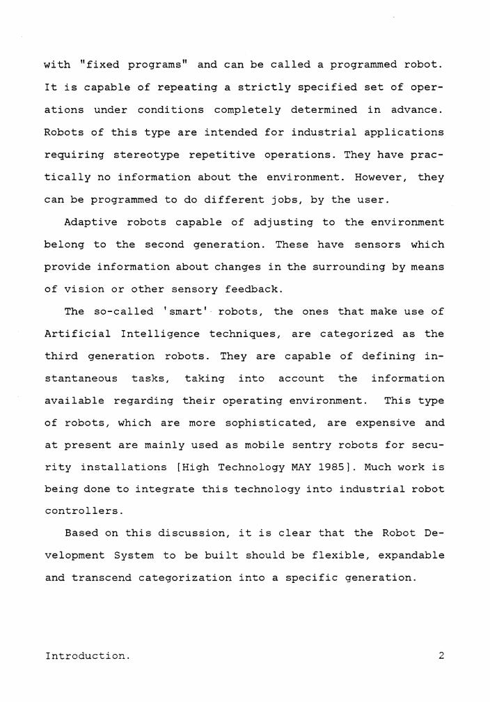
with "fixed programs" and can be called a programmed robot.

It is capable of repeating a strictly specified set of oper-

ations under conditions completely determined in advance.

Robots of this type are intended for industrial applications

requiring stereotype repetitive operations. They have prac-

tically no information about the environment. However, they

can be programmed to do different jobs, by the user.

Adaptive robots capable of adjusting to the environment

belong to the second generation. These have sensors which

provide information about changes in the surrounding by means

of vision or other sensory feedback.

The so-called 'smart'· robots, the ones that make use of

Artificial Intelligence techniques, are categorized as the

third generation robots. They are capable of defining in-

stantaneous tasks, taking into account the information

available regarding their operating environment. This type

of robots, which are more sophisticated, are expensive and

at present are mainly used as mobile sentry robots for secu-

rity installations [High Technology MAY 1985]. Much work is

being done to integrate this technology into industrial robot

controllers.

Based on this discussion, it is clear that the Robot De-

velopment System to be built should be flexible, expandable

and transcend categorization into a specific generation.

Introduction. 2

1. 2 SYSTEM REQUIREMENTS.

Before the design work began, the entire system was con-

ceptualized and the requirements for the RCDS (Robot Control

Development System) were clearly defined.

1. It should be possible to implement all the control algo-

rithms presently used by robots and provision should be

made to take into account future trends in control phi-

losophies.

2. The control structure should be modular to facilitate

easy modification, replacement or removal of different

control levels as explained later in this chapter.

3. Individual control of each joint must be available to the

user. This means, it should be possible to assign a dif-

ferent control structure to each axis of freedom.

4. System should be user friendly. The operator need not

know the actual system details to program a task. He/she

should be able to change all control constants and pa-

rameters in all the levels of control. If an unacceptable

constant is chosen, the system software must flash a

warning and go into a default mode to avoid damage or

injury. To lessen chances of a wrong entry, a menu

Introduction. 3

driven screen will be the interface between operator and

the machine.

5. If parts of a commercial robot are used to develop the

system, control should be easily transferable from the

original controller to the development system, and back .

. 1.3 THE CONTROL STRUCTURE.

Based on the system requirements, a hierarchical control

structure was chosen. This type of organization enables a

vertical integration of different control levels; each con-

trol level with wider aspect of the overall system than its

immediate lower level. A higher level will communicate with

the lower level, giving it instructions and at times receiv-

ing responses that help it to transmit the next instruction.

A structure like this allows for maximum flexibility and ex-

pandability. Maximum decoupling of hardware as well as soft-

ware is possible, enabling modular design of different

control levels and the communication between them. This also

provides for addition of more control levels at a later date

and removal or replacement of control levels with the minimum

of modifications.

The highest level is the man-machine interface level. At

this level, the operator programs the task and keeps track

of the data from the lower levels. The operator's decision

Introduction. 4

will always override the controller and so, emergency situ-

ations like collision avoidance will have to be controlled

at this level.

The remaining levels can be classified as follows [21].

• The highest level, after the user interface, is the one

that recognizes obstacles in the workspace by means of

external sensors.

• The next level is the strategical level that breaks down

the job/task into elementary moves of the tool center

point. Shifting and looping for repetitive operations are

done at this stage.

• The tactical level is usually the second from the lowest

level. Here trajectory planning, as discussed in chapter

two, takes place and the elemental displacements of each

joint with respect to time, is communicated to the lowest

level.

• Executive level forms the base of the hierarchy. This

lowest level is the servo system that executes the im-

posed motion of each degree of freedom. The task of the

executive level is the realization of a particular func-

tional movement. The basic control philosophy such as

Introduction. 5

Proportional Integral Derivative controller parameters

reside here.

1.4 SYSTEM OVERVIEW.

Instead of building the entire system from scratch, it was

decided to use the manipulator arm - the mechanical hardware,

actuators, feedback transducers and servo amplifier of an

available robot (General Electric P-50 process robot), as the

base, system.

The P-50 1 is an upgraded version of a welding robot and

is typical industrial robots. The controller supplied by the

manufacturer provides the user only with a restricted high

level command language to teach the robot different points

in the workspace. The robot can then be programmed to move

its Tool Center Point (TCP) through these points using ar-

ticulated, circular, or straight line motion. The speed of

the TCP can also be controlled. As such, the robot cannot

be used in research and development activities. The new

controller that was designed offers the user complete control

over the motion of each joint of the P-50.

To establish high speed computation at the highest control

level, a VAX 11/780 computer was the first choice. However,

l P-50 is the registered model number of the Process Robot marketed by General Electric, U.S.A.

Introduction. 6

due to geographical constraints, a hardwired line from the

VAX to the robotics laboratory was not available and the lo-

cal net, based on time sharing, cannot be tolerated in such

real-time dynamic systems. This prompted the use of an IBM

PC with 640 K Bytes of memory and an 8087 math coprocessor

to be used unti 1 something better becomes available at a

later date. The PC has an added advantage of easy availabil-

ity of inexpensive PC compatible hardware and software like

EPROM programmer, cross assembler for various microcontrol-

lers, and 8088, 8087 development systems.

It was decided to get the system working with three levels

-human interface, the tactical level and executive level -

and then add the other levels at a later date. In this three

level configuration, the IBM PC serves as the interface be-

tween the user and the system, as well as the tactical level.

A microcontroller for each joint forms the executive level

of the hierarchy. A survey of commonly available microcon-

trollers revealed the Intel 8031 to be ideal. The low cost,

availability as single board computers with serial and par-

allel ports, boolean operations at bit level, one micro sec-

ond instruction cycle, and multiply/divide instructions of

the I8031 made it the obvious choice. Chapter Four deals with

the system design and further details.

The executive level or the joint controllers are essen-

tially PID controllers. They receive position and velocity

feed back from each joint and send out a driving signal de-

Introduction. 7

pending on the reference position data and the actual posi-

tion. In order to design the software for this, the default

control parameters like Proportional Constant, Integral Con-

stant and Derivative Constant (K, K. and Kd) of P.I.D con-p l.

trol have to be determined, if the user prefers not to change

them. To do this, the weights and dimensions of each link was

measured and a highly simplified model of the robot was sim-

ulated on the computer using ISL ( Interactive Simulation

Language). Appendix B presents the results.

It must be pointed out that the model used, does not con-

sider the effect of gravity and friction on the coupled sys-

tern. The 'worst case', with the arm fully stretched

horizontally, is considered, as the intention was only to

arrive at approximate values for the constants.

The tactical level residing in the PC should compute joint

positions in real time or off-line computation mode. It was

decided that all computation be done prior to running the

robot and the data stored in a look-up table at this time.

When the robot is to be moved, the position data correspond-

ing to real-time situation is transmitted to each joint con-

troller which in turn executes the motion. The rate at which

the data is to be send and the position increments depend

entirely on the control algorithm used and the velocity with

which each joint is supposed to move.

Communication between the PC and the joint controllers are

through serial lines. This was selected as the mode of com-

Introduction. 8

munication since the PC can be replaced with a more powerful

computer without major modifications to the communication

protocol or the hardware of the joint controllers.

An EPROM programmer was procured as an integral part of

the system since different servo configurations for the

executive level can be stored as firmware on easily available

EPROMS that fit into the I8031 micro controller boards.

Since the original actuators and servo amplifiers of the

P-50 were used, it was necessary to find out where the feed-

back signals from the position encoders and the

tachogenerators could be tapped out. It was also necessary

to know the nature of the driving signal and where it could

be fed into the servo amplifier when the original controller

is disabled. This proved to be a difficult part of the

project. No schematics or other technical information were

available from the vendors since they were considered pro-

prietary information.

The only solution was to study the various signals on the

numerous circuit boards with an oscilloscope and to trace the

wiring on the printed circuits. This work was made all the

more difficult by the many custom designed hybrid circuits

that form the servo circuitry.

Finally, interface circuits were designed to decode and

condition the data from the position encoders and

tachogenerators. This data is the position and velocity

feedback to the joint controllers. A pulse width modulator

Introduction. 9

was built to give the acceptable driving signals to the servo

amplifiers of the P-50.

It must be stressed that this work has broken the ground

for further work on the Robot Control Development System. All

the hardware needed for one joint was designed and built.

They were tested as individual modules - position decoding,

velocity feed back and its analog to digital conversion, the

pulse modulator and the driving signal to the robot and the

serial communication between the joint controllers and the

IBM PC. These modules could not be integrated and tested due

to time constraints and the unforeseen break down of the ro-

bot. The software generated for this thesis was only for

testing individual parts of the joint controller and the

communication network.

The development of the entire software operating system

could be the topic of another thesis itself. A cross assem-

bler for the 8031 and a macro assembler for the 8088 were used

to develop some of the testing routines. The control algo-

rithm is meant to be written in a high level language, adding

to the user-friendliness of the system. Detailed schematics

required for constructing the remaining joint controllers are

included in the appendices.

Introduction. 10

2.0 KINEMATICS, TRAJECTORY PLANNING AND CONTROL OF

MANIPULATORS.

The purpose of a Robot system is to produce physical mo-

tion along the path prescribed by the user. Control of the

robot arm is required to maintain the specified motion of the

manipulator along a desired trajectory by applying corrective

compensation torque to the actuators to adjust for any devi-

ations of the manipulator from the planned trajectory

[12,15). Before any study or design of a robot controller

is undertaken, it is required to know the basics of robot

kinematics, dynamics and control. This chapter presents a

concise overview of these topics for a better understanding

of the present as well as the microprocessor based develop-

ment system for the P-50 robot.

2.1 HOMOGENEOUS TRANSFORMATIONS AND COORDINATE FRAMES.

Using the Denavit-Hartenberg representation of linkages a

simple yet efficient way of representing the position and

orientation of any link of a manipulator is presented

[28,16). Three dimensional coordinate frames with i,j and k

unit vectors as axes are assumed to be attached to each link

according to specified rules and from this, the orientation

Kinematics, Trajectory Planning and Control of Manipulators. 11

and position of one link with respect to another can be eas-

i 1 y computed. This will include a coordinate frame repres-

enting the inertial reference or ground.

A coordinate frame [C ] represents the coordinate frame n m "n" expressed relative to frame "m".

i n

0 0

k n

0

r on

1

Where in, k are 3Xl unit vectors representing the n orthogonal axes attached to frame n, whose components are

written relative to frame "m" and

r on is a vector from the origin of frame "m" to

the origin of frame "n".

This same matrix also known as "A" matrix can be inter-

preted as the one that transforms the frame "m" to frame "n".

[C l = [A l m m n [C ] is an identity matrix. m m

A transformation matrix [C] contains the complete infor-

mation needed to transform a coordinate frame from one lo-

cation and orientation to another. The upper left 3X3 sub

matrix of [C] gives the rotational information and the 4Xl

column vector, the last column of [CL

translational information of the frame.

Kinematics, Trajectory Planning and Control of Manipulators.

contains the

12

For a clearer presentation of how coordinate frames are

attached, consider Figure 1 on page 14 and Figure 2 on page

15.


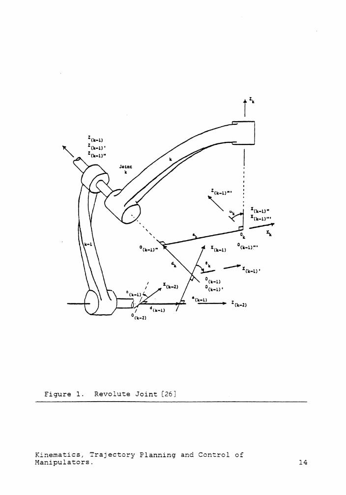
Figure 1.

%(k-l) %(k-1), %(k-1)"

Revolute Joint [26]

O (k•l) O(k-1)'

•ck-ll


1 Ck•l)" 1 (k•l)'" ___.

1c

14

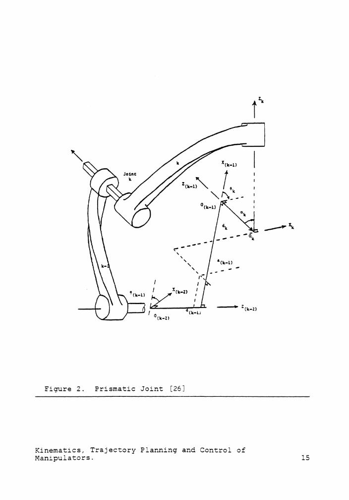
Figure 2. Prismatic Joint [26]


f

15

Figure 1 represents coordinate frames associated with a

revolute joint. The coordinate frames are attached to the

joint as follows.

1. The base or ground link is assigned the subscript 0.

2. The link attached to the base link is link 1 and the re-

maining links are numbered consecutively from the base

towards the tool center point (TCP).

3. The z axes are drawn along the joint axes and are as-

signed a subscript number, one less than the joint num-

ber.

4. Common perpendiculars to each pair of two axes are drawn.

These normals represent X-axes such that Xk is directed

If these axes intersect, orientation

of Xk is arbitrary or it can be in the direction of the

cross product+/- (Zk_ 1 ) X (Zk)

5. The Y-axes are defined by the right hand rule.

6. 0k is the directed angle from Xk-l to Xk measured around

Zk-l' positive by the right hand rule.


7. The twist angle ak is the directed angle from Zk-l to Zk

measured around Xk.

8. The perpendicular distance between Zk-l and Zk along Xk

is ak and is called the length of the link.

9. The signed number dk is the distance between Xk-l and Xk

along Zk-l and is positive in the direction of positive

10. The origin of the coordinate frames would be the inter-

section of corresponding X and Z axes.

11. The origin of the coordinate frame k would fall on the

intersection of Zk and Xk (along axis of joint k+l). If

Zk-l and Zk intersect each other, the origin would be at

the point of intersection of the two joint axes.

In the case of revolute joints (Figure 1 on page 14) 0 k is the joint variable and ak, dk, ak are the fixed quanti-

ties.

For prismatic joints (Figure 2 on page 15), dk is the

joint variable and ak, 0k, ak are fixed. To simplify the

matrix, ak can be made zero by relocating Zk-l as shown in

Figure 2 on page 15.


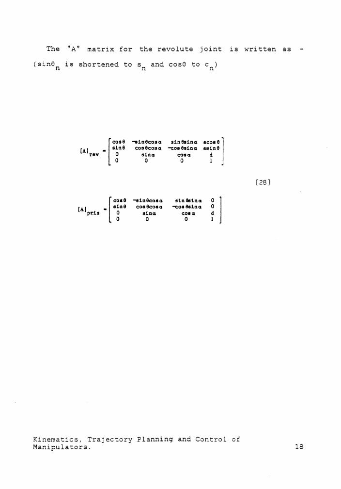
The "A" matrix for the revolute joint is written as

(sin0 is shortened to s and cos0 to c ) n n n

r~·· -sinecosa sin8sina acos el (Al rev

sine cosecosa -coaesina asine - 0 sina cosa d

0 0 0 l

[cosO -sinecosa si118sina 0 l (A]pris - sine cosecoaa -coseaina 0 0 sina coaa d 0 0 0 l


[28]

18

T

l ------- ---· "a

1'1•n.uJ.• I .. a I•'-~ IUB Jouc Cu-l

l I il . a 90 "t I l. I a : i2 . l6 0 a I 0 I L

J !3 . u 0 •3 0 I a I l.

• . 2• -90 •:. J I •l I 0

5 . ·5 . 90 90, I a 0 I l I 0 ., . 90 0 0 I ·; I 0 I

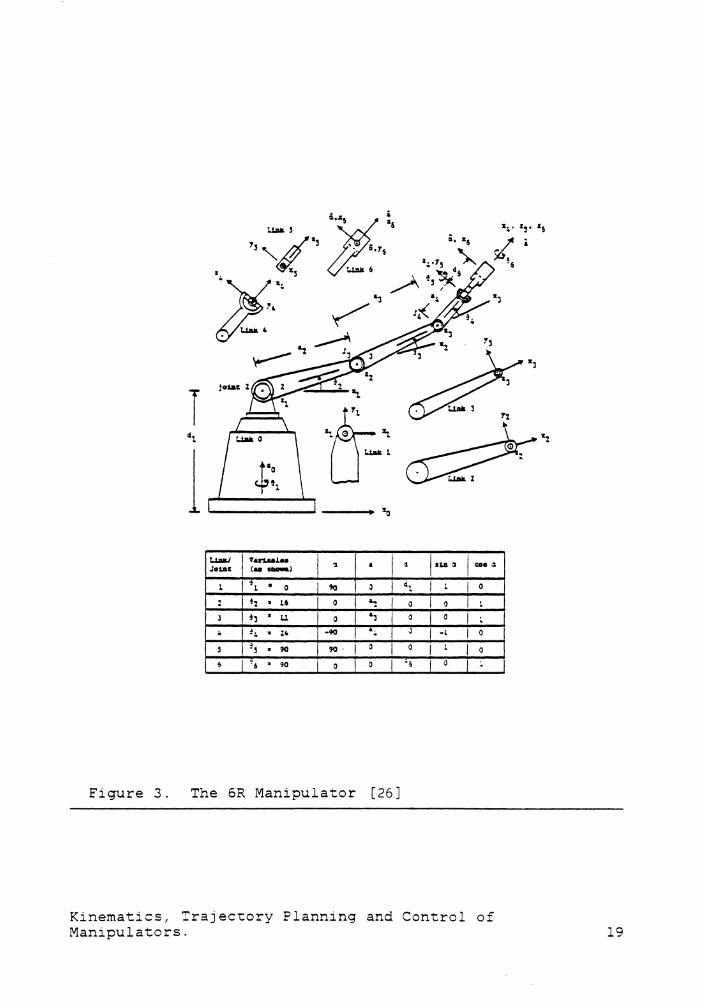
Figure 3. The 6R Manipulator [26]

Kinematics, Trajec~ory Planning and Control of Manipulators. 19

The 6R manipulator is shown in Figure 3 as an example of

how the coordinate frames are fixed and the elements of the

"C" matrix are computed.

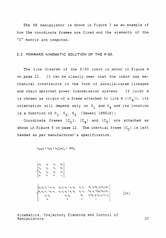
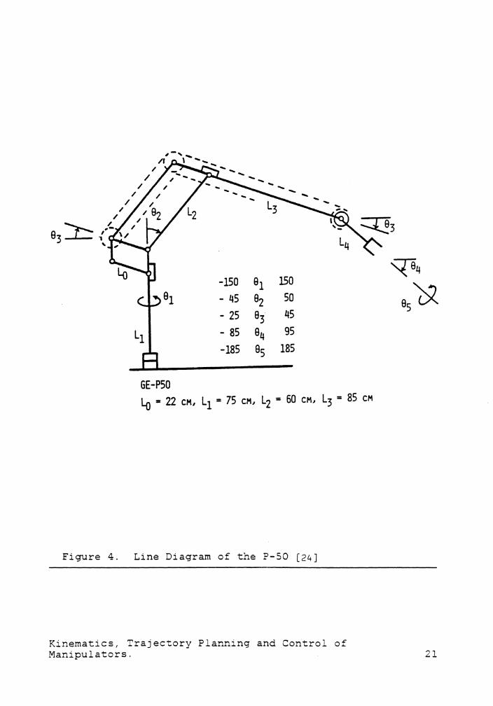
2.2 FORWARD KINEMATIC SOLUTION OF THE P-50.

The line diagram of the P-50 robot is shown in Figure 4

on page 21. It can be clearly seen that the robot has me-

chanical constr:-aints in the form of parallelogram linkages

and chain sprocket power transmission systems. If joint 4

is chosen as origin of a frame attached to link 4 ([C 4 ]), its

orientation will depend only on 0 1 and 0 4 and its location

is a function of 0 1 , 02 , 03 (Zewari 198S(b)].

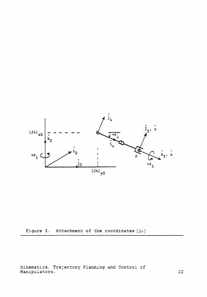
Coordinate frames [ c0 ], [ c4 ] and [ c5 ] are attached as

shown in Figure 5 on page 22. The inertial frame [C0 ] is left

handed as per manufacturer's specification.

.. .. .. p& . . y . y Py y .

' . '

. ' P,

0 0 0

s :5 t 4 s l • cl c, 1 4 , 1 c 5 - c:1 c 5 C:.4 1 1 (l,. c:4•.t2 •2~1i.:1)•1

I 5 S 4 C: 1 - I 1 C5 t 4 Ct C:5 + 1 l 1 5 c~ c:1 (l4 C4 •.t,•2+-½<1)cl

C:4 ., c4 C:5 .... .t1•12 c,-t) •3-14 '4

0 0 0


[24]

20

L4

-150 81 150 - 45 82 50 - 25 8 . 3 45 - 85 84 95 -185 85 185

GE-PS0 Lo= 22 CH1 Ll = 75 CH1 L2 = 60 CH, L3 = 85 CH

Figure 4. Line Diagram of the P-50 [24]


'(84

85iX

21

(J 4)zO

Figure 5. Attachment of the coordinates [24]


The last column of [ c5 ] 0 shows the location of the TCP

(Tool Center Point) and the third column the 'approach' of

the robot hand (axis z5 ). The first and second columns give

the 'normal' and 'orientation' vectors.

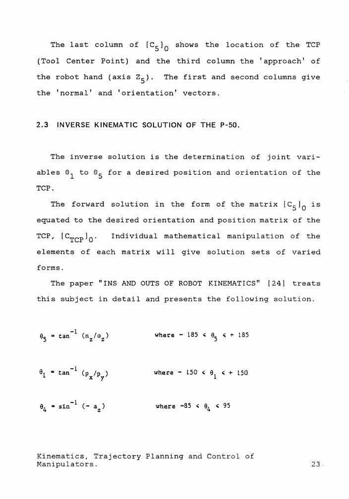
2.3 INVERSE KINEMATIC SOLUTION OF THE P-50.

The inverse solution is the determination of joint vari-

ables 0 1 to 05 for a desired position and orientation of the

TCP.

The forward solution in the form of the matrix [ c5 JO is

equated to the desired orientation and position matrix of the

Individual mathematical manipulation of the

elements of each matrix will give solution sets of varied

forms.

The paper "INS AND OUTS OF ROBOT KINEMATICS" [ 24] treats

this subject in detail and presents the following solution.

where - 185 < a5 ( + 185

where - 150 < a1 < + 150

a • sin- 1 (-a) 4 z where -85 ( e4 ( 95

Kinematics, Trajectory Planning and Control of Manipulators. 23.

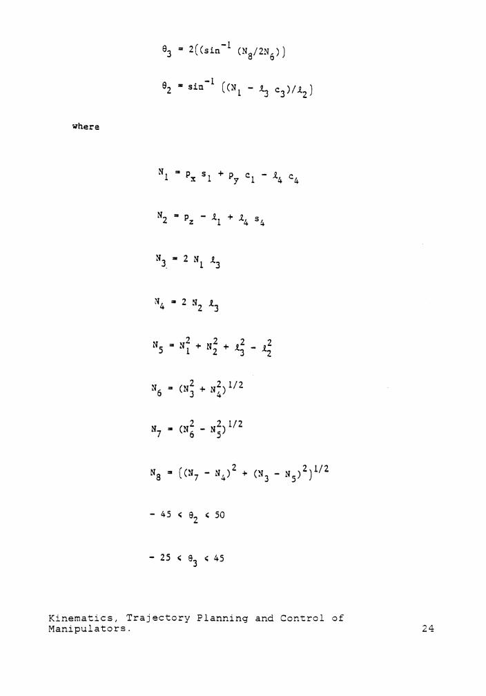
where

N l "' p s l + p cl - J.4 c X y 4


The forward linear velocities can be obtained by taking

the derivative of the position vectors. It must be noted

that although the TCP position and orientation is represented

as a 4X4 matrix, not all elements need be specified for

finding the inverse solution. The sum of the squares of the

components of each unit vector is one. This means only two

components of each unit vector need be specified. The cross

product of one component of a unit vector with the corre-

sponding component of another will give the component of the

third unit vector. Therefore, just by specifying the ele-

ments of the position vector and any four elements of the

upper 3X3 rotation sub-matrix, a computer program can deter-

mine the missing elements if needed and solve the inverse

kinematic equations to find the individual joint angles.

2.4 TRAJECTORY PLANNING.

While performing any task, the robot will move the Tool

Center Point from one specified location to another. The path

traced by the TCP between these two points is called the

trajectory. Trajectory planning is an important consider-

ation, especially in the case of painting and welding robots

where the movement of the TCP has to be under precise con-·

trol.


In a hierarchical control structure, as developed in

Chapter 1, trajectory planning is done in the level between

task computation level and the level that computes the in-

verse kinematic solutions. The trajectory planning program

usually divides the path between the present point and the

target point into small sections by adding intermediate

points along the path. These points are then used to compute

the inverse kinematic solution. The way in which these

intermediate points are selected depends on the trajectory

planning algorithm used or the individual 'joint-driving-

functions' [25].

The target point can be defined in two ways [10].

1. By the end point of the trajectory as defined by the task

program.

2. By a spatial displacement increment defined by its di-

rection and magnitude. Here, the target command is con-

tinuously changed in a random manner during the

trajectory interpolation. This method is usually employed

by Adaptive robots that have external sensors to guide

the TCP to the destination within a cluttered workspace.

When the path between the initial and final point is bro-

ken up into smaller parts or "splines" [ 23], the number of


splines depend on the location of work piece within the robot

workspace [23], precision of the path and complexity and ef-

ficiency of the algorithm used to compute the inverse

kinematic solution. Where precision is the main criterion,

more splines are required leading to greater amount of com-

putation which has an adverse effect on the speed of the TCP.

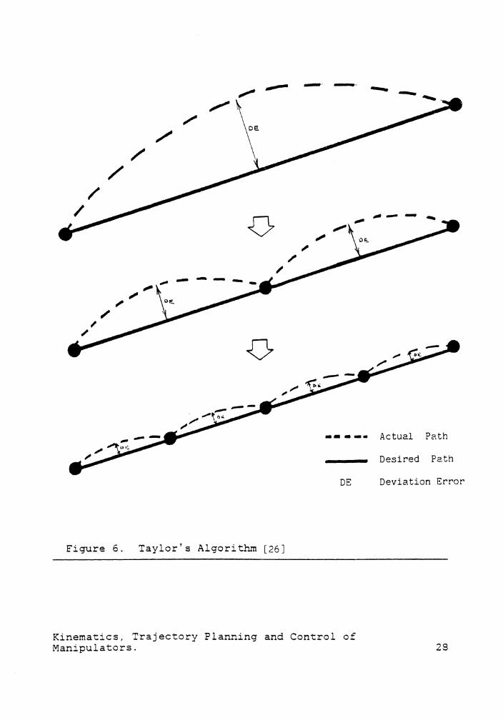
Taylor's algorithm is an example of how straight line

trajectory can be implemented. This algorithm determines the

distance between the location of the TCP at joint space mid

point and the straight line mid point (Figure 6 on page 28).

If this deviation is unacceptable, the mid point of the de-

-sired straight line path is selected as an intermediate node

and the path is divided into two splines. This algorithm is

run recursively util an acceptable deviation from the path

is reached.

One way of implementing such an algorithm in real-time is

to ignore the magnitude of deviation from the straight line.

The precision of the trajectory will depend on desired robot

speed and the speed of the computer. The computer can first

of all compute the number of times it can calculate the in-

verse kinematic solution within the time given for the TCP

to move from one point to the other. The number of splines

or segments into which the path can be broken up will be equal

to this number, no matter what the deviations are.


,,,- --------

•• • -• Actual Path

Desired Pa.th

DE Deviation Error

Figure 6. Taylor's Algorithm [26]


It must be noted that the trajectory need not always be

computed in real time. One common method is to have the pro-

gramming done off-line and the trajectory and inverse

kinematic calculations results stored in a look-up table in

the memory of the computer. When the robot is running, data

from the table can be fed to the joint controllers in real-

time.

Another method of accomplishing off-line programming is

to move the TCP over the required path manually, while the

joint positions are sampled and recorded at a fast rate.

These taught points can be 'played-back' at different veloc-

ities in real-time, as practiced in painting robots.

Both of the above methods preclude the use of vision or

other sensory feedback during operation of the robot and

hence are not suitable for adaptive control.

2.5 JOINT DRIVING FUNCTIONS.

When trajectory planning of the TCP is the main concern,

little attention is paid to the motion of the individual

joints. If the TCP is made to move in a straight line, in-

variably, the joints will be subjected to impulsive forces

that expedite the breakdown of the mechanical components.

In operations like 'pick-and-place' where the path of the TCP


is not of much importance, the joints can be driven with

special joint driving functions to reduce the wear and tear.

Currently, a variety of joint driving functions are in

vogue [25]. Some of them are described below.

1. Bang-Bang is misleadingly referred to as constant accel-

eration, constant deceleration driving function in

robotic work. This function is highly impulsive at the

boundaries and at midrange and should not be used in

driving actual robot joints except for comparison with

other functions.

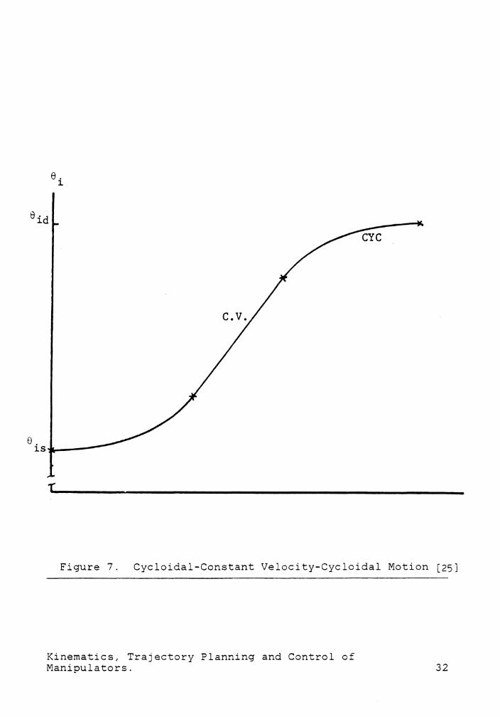
2. Third order polynomials. The position of the joint is

written as a third order function of time. As can be seen

from figure 2.8, the start point and end point are sub-

ject to abrupt change in angular acceleration which leads

to impulsive forces.

3. Fifth order polynomials. These are popular joint driving

functions. Their advantage being the ability to start

executing another segment of motion before coming to a

full stop. This is because the acceleration and velocity

at the boundary regions need not be zero. The disadvan-

tage is the longer computation time required.


4. Joint space interpolation. In this method, all the joints

start and stop at the same time. Their velocities are

constant during motion leading to large impulsive forces

at the end points.

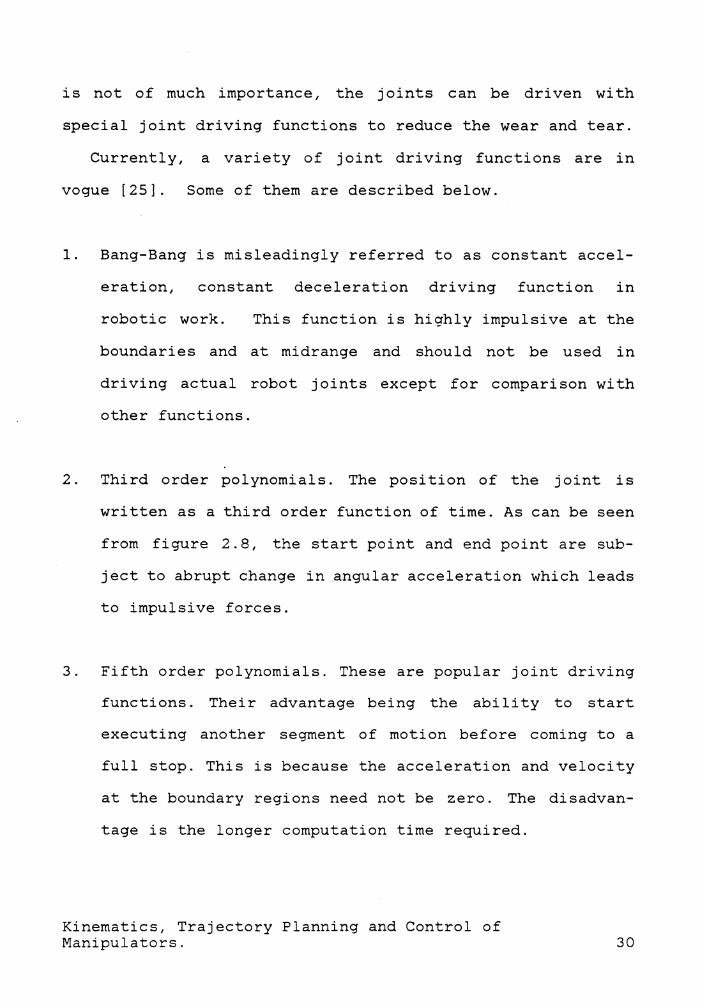
5. Cycloidal-constant velocity-cycloidal motion. This mo-

tion is best explained by Figure 7 on page 32. The con-

stant velocity part of this function reduces the peak

power required to move the joint. The computation re-

quired might be higher than the fifth order or higher

polynomials.

Figure 8 on page 33- shows a comparison of the velocity

vs. time and Figure 9 on page 34, has acceleration vs. time

for the different driving functions. A study of these plots

show the fifth order polynomial driving function to provide

the smoothest motion. A detailed mathematical study of these

driving functions and their effect on the joints of robots

could be the topic of another thesis. The results presented

in this section represent the work done in the Dept. of Me-

chanical Engineering [25,26].


e . 1

0 . 1s..,.------

Figure 7. Cycloidal-Constant Velocity-Cycloidal Motion [25]


~:;,<: Ill 1-'· pp ..... (1) 'd 9

Ill I-' rt Ill 1--'· rt () 0 (I}

tf -(I}

H 1-1 Ill

LJ. (1) () rt 0 tf '<

w w

tu I-' Ill p p ...... p ,Q

Ill p p.

0 0 p rt 1-1 0 I-'

0 H)

"1 ......

1-1 (1)

00

<! (1) I-' 0 () ...... rt '< <: (I}

rt ...... ;3 (1)

.. N V1 ._,

Bl IR

Ill IR

IQ ::I(\· ..... u 0 .JBI W, >m -.... t-,IR o· ·1!2

8

JI VELOCITY lOEG/SECl

+ ••• lRST ORDER POLY. x ••. 3RO ORDER POLY. •... STH ORDER POLY. -••• BANG - BANG z ••. CCC FUNCTION

·--~---,r----r----r----.----,.-----r----,-----,------• II .22 .93 .44 .B:i

NORMALIZED TIME

C)

U) . u u.J

U)

' 0 u.J C

l

J u.J u u a:. --,

• >-

J J

00 Z

a..a..oo z-

a: a: CI t-

W LLJ C

D U

C

lCl

Z 0: a::

I ::,

0 0

LL 0

Cl l:

Z U

0:1-C

IU

m U

J CD

U

. . I

e I

e . . . . . X

•

I N

a -Lu

-a Lu N

-..J ,;a:

'%:

a:: 0 z

m .

--0 1

K

, 1

, ::::::,,,._.

• ,

I 00•

21·0-r,-·,s

ct:sr oo·a

a,:s:-,,.·1E-

zt·~ N

O I lt:;~373::J'Jtj Ir

Figure 9.

Accleration

vs. tim

e [25]

Kinem

atics, Trajectory

Planning and

Control

of M

anipulators. 34

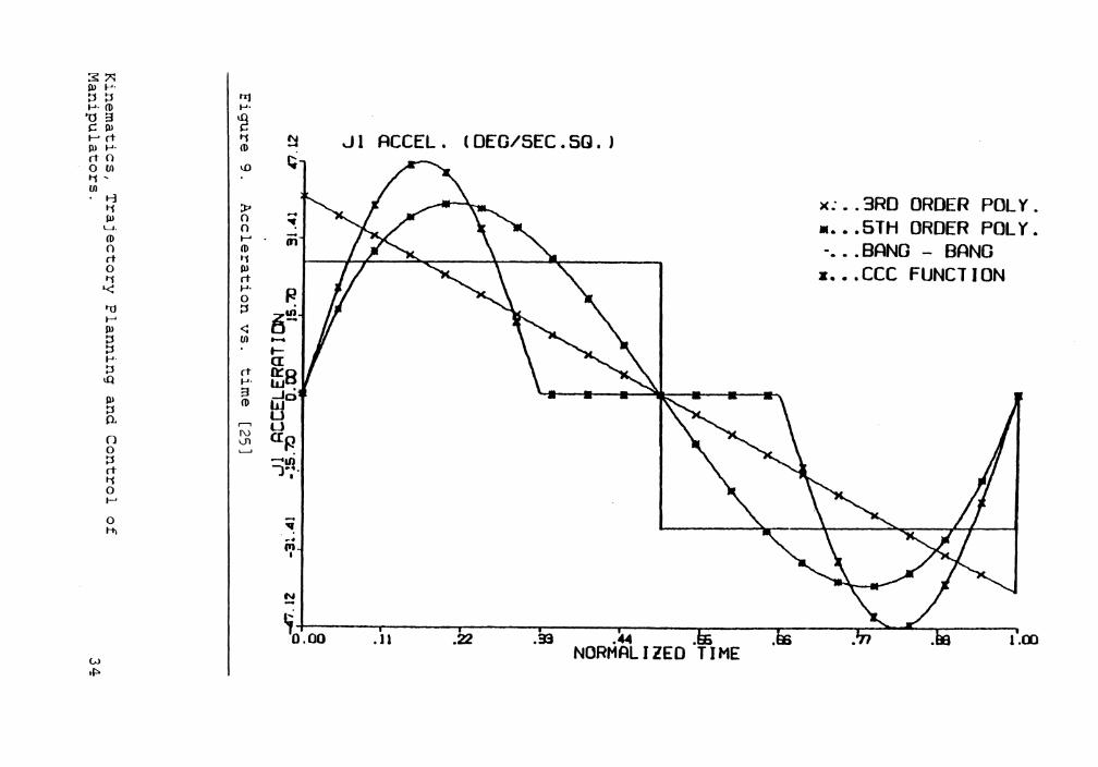
2.6 CONTROL OF THE ROBOT.

The design of a control system for a robot depends on a

number of factors [17).

1. The geometric design of the machine.

2. Specifications of speed and accuracy.

3. Type and structure of task to be performed.

4. External disturbances.

5. Accuracy in modelling the arm.

6. Method of teaching the task.

For a robot to perform well, full coordinated control of

each degree of freedom has to be effected by sophisticated

control algorithms. These algorithms take into account the

kinematics and dynamics of the system and compute the forces

and torques needed to drive the TCP along the desired tra-

jectory. Though this may be considered the 'Control-

Problem', the solution for manipulator control is complicated


by the gravitational loading of the arms, friction and the

coupling reaction between the joints.

Many control methods have been established [ 13] and in

fact this work is itself the development of a system to serve

as a tool for developing and testing different control phi-

losophies. The prominent control methods used today are the

Resolved Motion Rate Control (RMRC) [22], the Cerebellar

Model Articulation Control ( CMAC), Near-minimum-time con-

trol, the Computed Torque method and the Adaptive Control

techniques.

The RMRC is a technique by which the joint angle rates

required for the TCP to move in a certain direction with

respect to the inertial coordinate system is computed. To

find the angular velocities, the inverse of the Jacobian Ma-

trix is required and this computational effort and ocassional

singularity of the Jacobian matrix are the main disadvantages

of this method.

Cerebellar Model Articulation is a table look up control

method based on neurophysiological theory. Instead of solving

analytical equations, control functions are computed by

looking up a table stored in the computer memory.

Near-minimum technique is based on the linearisation of

the highly non-linear motion of the robot, around the nominal

trajectory and linear feedback is obtained analytically. For


manipulators with more than four joints this proves to be too

complex [ 13] .

Adaptive control methods can be used to maintain good

performance over a wide range of motions and payloads. Sta-

bility is the problem here since the dynamic equations of the

manipulator are complex arid non-linear. A good simulation

model is difficult to device and designing a stable adaptive

control law is neither simple nor easy.

The computed torque technique assumes that all the dynamic

and kinematic parameters of the manipulator are known. From

this, the driving signal required to move a joint from one

position to another with a particular velocity is computed

and applied. This is basically a feed forward system that

does not take into account the changes in payload or any ex-

ternal disturbances. An off shoot of this method is the Dual

Mode Control scheme which combines the inverse dynamics with

servo feedback [27). Here, the computed torque method is em-

ployed in conjunction with a servo feedback loop or until a

particular time when control is switched to a feed back servo

system. This way the steady state error inherent to the com-

puted torque method and the initial oscillations of a servo

are avoided. The main problem with the later version of this

scheme is determination of an optimum moment to switch over

to the servo.


This brief discussion on different control strategies is

in no way comprehensive. It gives a general idea of the con-

trol problem and shows the need for a robot research tool to

provide for experimental verification of different control

schemes. This chapter also shows the computational power

required of a robot controller.


3.0 STUDY OF THE P-50 ROBOT.

The Robotics Industry Directory [20] describes the P-50

as a continuous path, five degrees of freedom, point to point

linear interpolation process robot with a resolution of

0.2mm, accuracy of 0.2mm and a repeatability of 0.2mm. This

robot is manufactured by Hitachi Corporation of Japan and

marketed in the United States by General Electric. The P-50

is an upgraded welding robot with a load carrying capacity

of 10kg. Its typical applications, supported by the manufac-

turer, are machine tool loading/ unloading, parts transfer,

spray painting, plastic molding and welding.

3.1 SYSTEM CONFIGURATION.

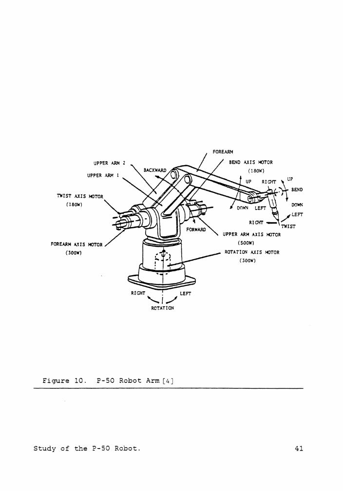
The main components [5] that make up the P-50 are

• The Robot Body. This part is the floor-mounted five axis

arm. The rotation unit, upper and forearm drive unit,

wrist drive unit, forearm rear unit and the forearm tip

unit make up the whole arm. Figure 10 on page 41 shows

a sketch of the robot arm and the different axes of

freedom. The rotation, upper arm and forearm axes are

driven directly by DC servo motors through harmonic

drives. In the case of the bend and twist axes, a system

Study of the P-50 Robot. 39

of chains and rigid bars are used along with the harmonic

drives to transfer the power from the actuators. The

rotation, upper arm and forearm axes motors are equipped

with electromechanical brakes for holding the arm in po-

sition when the servo system is deactivated. Each of

these axes are also equipped with proximity switches

which lets the controller unit determine the zero point

or the reference point. Figure 11 on page 42 gives the

specifications of the robot body [4].

• Controller Unit. The controller contains all the elec-

trical and electronics required to program, store and run

the robot. It also has the interfaces for input/output

functions and for operator communication. This is the

part that is being replaced by the development system.

Since the bubble memory and the analog servo circuits are

sensitive to electrical transients, an isolation trans-

former is used to protect it form any transient surge in

the incoming power line.

• The Teach Box. This is a portable "pendant" with membrane

keyboard. It is used as a portable programming unit that

determines the direction of robot arm movement and sets

various control conditions under which the movement is

to be performed. The teach box is connected to the con-

trol~er unit.


UPPER ARM 2

UPPER AAA 1

TWIST AXIS MOTOR (180W)

FOREARM A.~IS MOTOR (lOOW)

RIGHT . LEFT

"-.I/ ROTATION

Figure 10. P-50 Robot Arm [ 4]

Study of the P-50 Robot.

SEND AXIS MOTOR ( 180W)

RIGITT ~IJP

rt'~~=-~~• SEND o.-~....-. __,,,LL.._

DOWN

/LEFT

TWIST UPPER ARM AXIS 1-0TOR

(SOOW)

ROTATION AXIS MOTOR (300W)

41

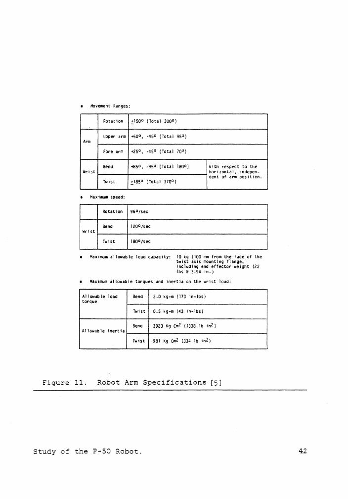
• Movement Ranges:

Ro tat ion +150° (Total 3000)

Upper arm +5QO, -450 (Tota I 95°) Arm

Fore arm +25°. -45° (Tota I 70°)

Bend +850, -950 (Total 1800) With respect to the Wrist hOrizontal, indepen-

dent of arm position. Twist +185° (Total 370°)

• Maxi,rum speed:

Rotation 960/sec

Bend 12001sec Wrist

Twist 1800/sec

• Maximum allowable load capacity: 10 kg (JOO mm from the face of the twist axis mounting flange, including end effector weight (22 lbs @ 3.94 in.)

• Maximum allowable torques and inertia on the wrist load:

Allowable load Bend 2.0 kg-m (173 in-lbs) torque

Twist 0.5 kg-m {43 1n-lbs)

Bend 3923 Kg cm2 (1338 lb in2) Allowable inertia

Twist 981 Kg cm2 (334 lb in2)

Figure 11. Robot Arm Specifications [5]


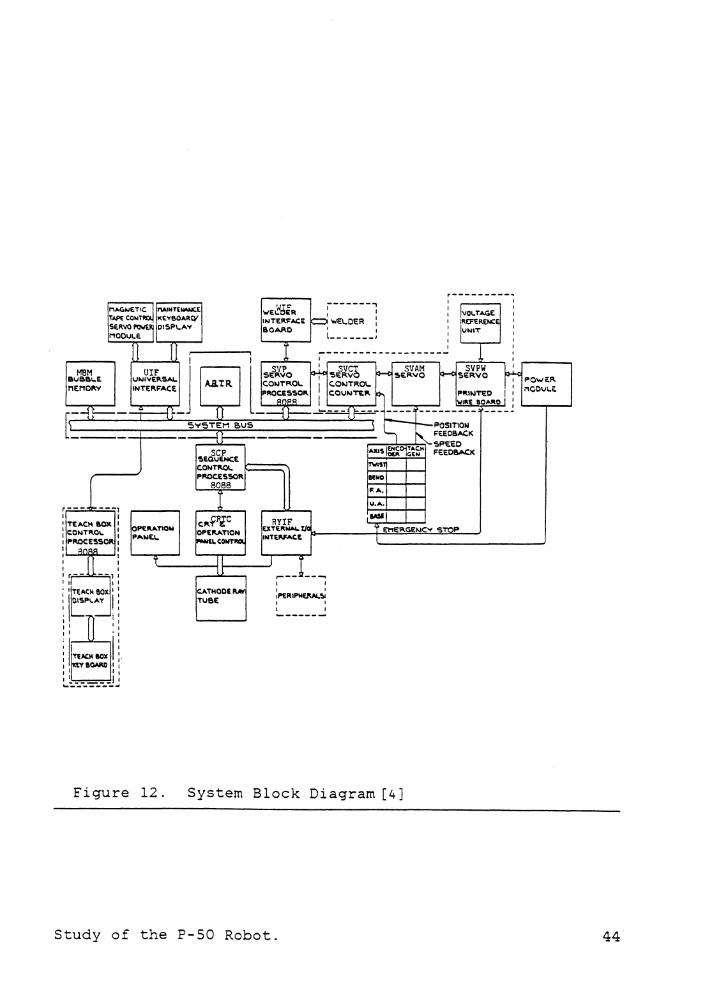
3.2 WORKING OF THE CONTROLLER.

Schematics of the electronic circuitry of the controller

or any other techical information about it is considered

proprietary. Hence a general idea of how the controller works

was culled from the system block diagram (Figure 12 on page

45 ) supplied by the venders and by observing signals at

various points on the circuit boards with an oscilloscope.

The first thing that is observed when the controller cir-

cuit board is exposed is that all the signals and data are

transmitted via two wire differential lines. In the mainte-

nance and installation manual the letters P and N are used

to denote the two wires assigned to each signal. This tech-

nique is used to develop immunity from electrical noise. The

servo pulse amplifiers and welding machines generate so much

electrical noise that it would cause havoc in the digital and

analog circuits of the controller. Noise is picked up by

wires carrying signals. Since differential lines are used

only the difference in voltage levels between the two lines

are considered as the actual signal. This will totally elim-

inate all the noise picked up because the noise levels on

both lines are the same.

Once the front panel of the controller is removed, a se-

ries of circuit boards can be seen mounted on the 'W-rack'.

These circuit boards bear a one to one relationship with the

blocks on Figure 12 on page 1)!5. wt.


MAGWE.TIC. MINTE:»'NC.E !TAP£ co .. no KEY80AR[V SERVO ~I CISPI.AV MODULE

wE2idiR INTERFACE 110"-RO

-------, I I

ioWELCER : ' I (_ ______ ,

r--------- .. I I I I

' VOLTAGE I

' RO'e.RENC:£ I I UNIT I I I I I

] I J I __ ..,__~ ;-r-------------~-- --r----_-_-_-_-..,----"'----, :

j l SI/P I SVCT SVAM SI/PW r: l I I

MBM euae.1.E MEMOfl.V

UIF SEF\VO SERVO jO-< SEFWO SERVO I PO'-'C:R u,NNT,:RE~!c"; AB.1:R. coNTR01. I CONTROi.. , _

.. •. .. PROCESSOI\ COUNTEF\ PIO.INTED I I ncou1. .. 0 ~ 00 I '--~---' ._ __ ,_,_ w11'r acA"O i : ----,----

[\_--n--_ -- ri-- 11 --n--=--=-=-f!==-- .::-- -------- ~-----,, S.,.STEt1 BUS I r-POSITION

•--l f---------•---- I f'_ FEEOa.t.CK -+---·- SPEEO

, ___ 1 ___ 1

I I 1 TtACH 80X I : CONTI0.01. : 1 l'IO.OCE5SOR 1 1 MM I

SCP SEQUENCt CONTI\OI. ~==:"\ PIIOC.ESSOR

8088

I

A1U$ 1~°1~~~M FEE08ACJ<

ltNO

F'.A.

U.A.

c,._f?iC OPEIO.ATION Jl'N,u COIITIOIIO

,IASI afU.f.... tic 't El"IERGe:Ncv STOP INTEI\FACE "l:1-------,Jr--"====-=="---'

I 1 : ~--n--,: t ii 11

't'------,![1---_,1 ~--!--~ . '!~:cw SOX I I

ILPl.:_!i §', :I T(KH SOX i i

'l'IIOAIO.Cl1 I l 1

~-----l I ________ _,

Figure 12.

CATHODE RM TUBE

1 I I I 11'ERIPMEIVll.!ol

System Block Diagram [4]


There are two CPUY boards; the SCP and SVP. These are t·wo

identical CPU boards with the 8088 microprocessor as the

central processing unit. The other LSI chips on this board

are a programmable interrupt controller 8259, a universal

asynchronous receiver/ transmitter 8251 for the serial com-

munication, an 8253 timer and an 8255 PIO (parallel input/

output) chip. The only difference between the SVP and SCP

boards are a set of differently set DIP switches. The system

monitor is placed in two eproms. The labels on the eproms on

the two circuit boards bear the same code, indicating that

the system monitor is also the same. Only the operating en-

vironment is changed by the settings of the DIP switches. The

sixty line finger connector at the edge of these cards plug

directly into the mother board which bears the main system

bus and the Bus Arbitrator. The job of the bus arbitrator is

to prevent contention of the bus between all the circuit

boards. A close study of the Mother Board connection diagram

(page 8.17 of the maintenance and installation manual) shows

that the finger connectors carry only the address and data

lines along with the power supply lines (+5V,+12V,-12V,Analog

Ground and Digital Ground). There are two edge connecters

on the outer edge of these boards. One of them brings out two

eight bit parallel port lines as well as the data bus. The

other is a serial port. All these observations lead one to

believe that the SCP and SVP are in effect single board com-

puters.


The parallel port and data lines from the SVP connect to

the SVCT or servo counter board. The serial lines are con-

nected to the welder interface board or WIF. SVCT or the

servo counter board is the only digital portion of the servo

circuitry. The inputs to this board are the digital data from

the SVP and the position feedback from the position encoders

of each joint. The output from the SVCT are a set of digital

lines marked VCO through VCll. In servo control parlance, the

position error signal is also called the velocity control

signal. From this it can be hypothesized that the SVP feeds

the position reference signal to the SVCT which conditions

and subtracts the actual position from the reference to get

the velocity control signal in 12 bit data format. It must

be noted that both the reference position input as well as

the velocity control output are time division multiplexed.

To decode the multiplexed signals, lines carrying the decod-

ing information are also supplied from one board to another.

SVAM is the name of the sevo amplifier or the analog part

of the servo circuitry. The inputs to this board are the ve-

locity control signals which are converted to analog data by

a D/A converter and demultiplexed; and the actual velocity

feedback from the tachogenerators attached to the shaft of

each actuator. There are five sealed hybrid micro circuits

on this board that determine the velocity error and send out

the driving signal. The output from this board is the driv-


ing signal in a pulse width modulated form, one for each de-

gree of freedom.

The SCP board, the other CPU board, has its parallel port

lines connected to the RYIF board. The RYIF board is the one

that takes care of all the external input/ output signals.

This board has banks of electromechanical relays that isolate

the electronics of the controller from external voltage

sources. There are also a set of timer ICs on this board. The

use of these I/0 lines can be explained as follows.

1. Input signal - Used as an interlock signal from a pe-

ripheral device to change the operating condition of the

robot or to stop/start robot motion.

2. Output signal-Used as a start signal for the peripheral

unit, from the robot. The peripheral unit can also be

controlled by the robot to a certain extent by using a

set of output lines to format a digital word and having

some electronics on the peripheral side to decode the

'meaning' of the word.

3. Timer - Used as a time limiting element for both the ro-

bot and the peripheral unit.

There are sixteen input lines and sixteen output lines


The serial port of the SCP board is connected to the CRTC.

This is nothing but the cathode ray tube controller. The

circuitry is similar to that of a video monitor. The data

coming in through the serial port is displayed on the CRT

screen. There are some optional output ports from this port

which can be used to run a printer.

UIF and MBM are the remaining circuit boards on the W-

rack. The UIF is a kind of universal interface board that

interfaces the Maintenance Keyboard (MKD) and the cassette

deck to the main system bus. To mention briefly about the

MKD, it is a keyboard and led display which can be used to

pinpoint faults and to rectify software faults in the case

of a breakdown. It is used to load system software from cas-

settes to the bubble memory. The MBM board has an onboard

DC to DC converter that takes in the +SV and -12V lines and

outputs a higher voltage needed by the magnetic bubble mem-

ory. The bubble memory is a technique of storing large den-

sities of data in a non-volatile form without the use of

moving parts. Usually rare earth garnets are used as the base

for making bubble memories. These materials have the prop-

erty of being able to trap magnetic domains within their

surface. The magnetic domains shrink into cylinders or 'bub-

bles' [2] when an external magnetic field is applied. With

suitable 'islands' of magnetic material placed on the surface

of the garnet and by means of conductors which generate a

revolving magnetic field, these bubbles can be moved around


within the material. If the presence of a bubble in a certain

location indicates a logical one and its absence a zero,

digital data can easily be stored. The technique of reading

the presence, creation and movement of a bubble is complex

and beyond the scope of this chapter. All that is required

to be known from the controller point of view is that the

magnetic bubble memory board acts as a non-volatile 128K byte

RAM. It may be mentioned in the passing that these devices

are extremely sensitive to transients in the supply voltages

and to external magnetic or electric fields.

SVPW is the servo pulse width modulator. This board can

be seen only if the back panel of the controller is laid back

on its hinges. Care should be taken while doing this since

two of the flat cables are not long enough and they have to

be detached from the connectors on the SVPW board. The only

input to this board are from the SVAM, the driving signals

for each joint, the brake control lines and servo on/ off

line. There are some interlock circuitry built into this

board to switch off power supply to the power amplifier if

conditions like over-current or damage to the power devices

occur.

The driving signal from the SVAM is an 18.658kHz pulse,

varying in amplitude from -2.Sv to +2.Sv. This signal and its

generation are discussed in the next chapter. The heavy-duty

de current for each motor is pulse modulated by the driving

signal. During the negative half of the pulse, current passes


through the motor in one direction. The positive half sends

the current in the opposite direction. The motors are of the

permanent magnet direct current type. Due to the high fre-

quency of the alternating current, the shaft remains sta-

tionary. To rotate the motor shaft in any one direction, the

duty cycle (the percentage of the period of the pulse for

which it is positive) of the pulses are changed. When the

duty cycle is less than 50%, there is more current passing

in the negative direction and the shaft rotates in that di-

rection. Similarly, with a duty cycle greater than 50%, ro-

tation is effected in the opposite direction. The motors,

being of the permanent magnet type, do not have the problem

of cross magnetization effects and empirically, the re-

lationship between the duty cycle of the driving signal and

the motor torque can be deduced as follows.

• 0% duty cycle equivalent to 100% torque in negative di-

rection.

• 50% duty cycle equivalent to no torque in either direc-

tion.

• 100% duty cycle equivalent to 100% torque in positive

direction.


Because of the bui 1 t in current feedback loop in the power

module (pulse amplifier) there is a linear relationship be-

tween the torque and duty cycle for all practical purposes.

Note that inductors are connected in series with the motors

to reduce the current pulsations in the motor drive circuit.

Al though the rated voltages of the motors are from 85V to

115V, all of them are driven from a lOOV DC bus. Figure 13

on page 52 gives all the parameters of the actuators.

As a protection measure, the servo goes into an emergency

stop if any fault is detected by the interlock circuits. In

the case of minor errors, the operator can reset the system,

however if the error is major ( as determined by the CPUY

cards), the power supply to the entire system will have to

be switched off, the error rectified and the system re-

powered. Techniques for overcoming these interlocks for

disabling the present controller without affecting the pulse

amplifiers are explained in the chapter on system design.

3.3 CONTROL STRUCTURE OF THE P-50.

From the above discussion on the working of the controller

it can be concluded that the controller emulates a four level

hierarchical control structure. The power modules, SVPW,

SVAM, and SVCT make up the lowest or the executive level. The

SVP and MBM boards form the tactical as well as the strate-

gical levels ( as discussed in the introduction). Certain


NAME MOTOR SIZE MOTOR REVOLUTION AXIS MOVING END

Rotation O.JOkW cw Left ccw Right

Upper Ann O.SOkW cw Rear ccw Fore

Foreann O.JOkW cw Down ccw Up

Bend D. 18kW cw Up ccw Down

Twist 0. 18kW cw Right ccw Left

Motor rewlution directions indicated In the above table were detennined when looking at the motor from the drive shaft end.

The output shaft of each hannonic drive moves in~ direction opposite to that of the motor.

~otor revolution: CW: Clockwise CCW: Counterclockwise

Figure 13. Servo motor specifications [4]


amount of adaptiveness is possible with the input output

lines and the SCP RYIF combination could be considered as the

fourth level of the hierarchy, from the bottom. The man -

machine interface is accomplished by the CRT display, the

controller keyboard and the teach box.


4.0 SYSTEM DESIGN.

This chapter deals with the design and development of the

development system for the P-50 Process Robot. As mentioned

earlier in the introduction, the goal was to provide for the

disabling of the original controller and to transfer control

of the manipulator arm to the new development system. How-

ever, to avoid duplication of hardware, the power amplifier

of the original controller is used in the design of the new

controller. Al though the entire Robot Control Development

System was conceptualized, only the hardware for the execu-

tive level and the communication link to the higher levels

could be built and tested. This in itself is no mean

achievement since, at the start of the project, there was no

technical information available on the P-50 and all the

interface hardware and software had to be designed and tested

in a sort of trial and error fashion. In this chapter, em-

phasis is placed on the work that has been done. The rest can

be considered as guide lines for developing the entire sys-

tem.

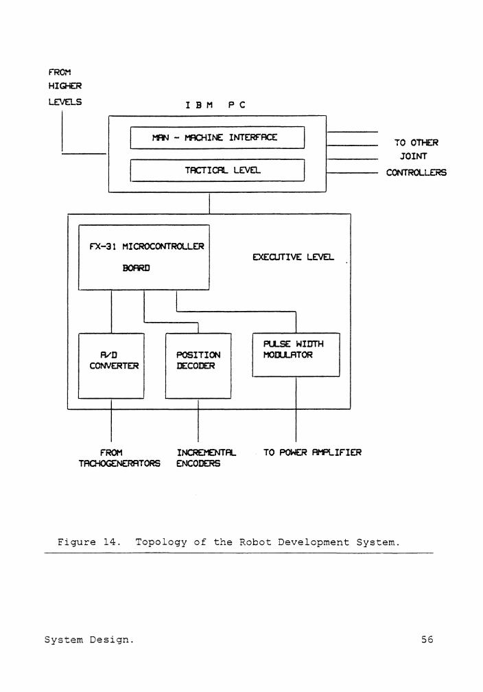
4.1 SYSTEM TOPOLOGY.

With the hardware presently available, a four level control

hierarchy is envisioned. The IBM PC integrates the human

System Design. 54

interface through its keyboard and color monitor, the stra-

tegical level and tactical level in a high level language

like FORTRAN and the communications to the executive level

through serial ports. Figure 14 on page 56 shows the ar-

rangement of the different levels of the control hierarchy.

The executive level is made up of five different microcon-

trollers. All of them operate independent of each other.

These microcontrollers get feedback signals from the manipu-

lator and the reference or 'set point' from the tactical

level in the IBM PC; their output is the driving signal to

the power amplifier of the P-50.

4.2 THE DIGITAL SERVO.

To begin at the lowest level of control, the executive

level can be split into four sections for a detailed study.

These sections are:

• The micro controller board .

• Position decoding circuitry .

• Velocity feedback signal .

• Driving signal generator .

System Design. 55

FROM HIGHER LEVELS I B M P C

I l'ff,.I - l"R:HINE INTERF"ACE I I TRCTICR. LEVEL I

F"X-31 MICROCONTROLLE:R EXECJTIVE LEVEL

BOARD

I PU.SE WIDTH

A/D POSITION MOill.ATOR CONVERTER DECODER

f"ROM INCRDOITFL TO POWER Al"A..If"IER TROIOG£NERATORS ENCODERS

TO OTHER JOINT

CONTROLLE:RS

Figure 14. Topology of the Robot Development System.

System Design. 56

Various control structures were considered for this level.

The simplest one utilizing all the feedback resources avail-

able was to be implemented at first, to test the servo and

then it is to be left to the researcher to develop any par-

ticular design, in the assembly language of the microcon-

troller used, to suit their research needs. Considering a

simple proportional controller, the equation could be written

as

DCP =(KP* DE)

where, DCP = proportional controller output

DE = the error

KP = proportional gain.

The disadvantage with the proportional controller is its in-

herent steady state error problem. Its equation shows that

the power applied to the motor is equal to a constant multi-

plied by the error. Now, for the arm to hold a load against

gravity requires a torque output from the motor. But if there

is no position error, there can be no torque and hence a

steady state error is inherent in this control configuration

to hold up a load or compensate for sustained disturbance.

The second problem with proportional controllers is over-

shoot. The joint has only friction to stop its movement. If

that frictional force is small, the joint will tend to over-

shoot the desired position and if its too large it may never

get to the desired set point.

System Design. 57

To avoid the steady state error problem, an integrating

controller could be added. The equation of a Proportional

Integral controller can be simplified and written as

DCPI =(KI* SUM* DT) + (KP*DE)

where DCPI= controller output

SUM= SUM+DE = summation of all the sampled errors

KI = integral controller constant

DT = time between samples

SUM*DT= area under the error-time curve.

The Proportional Integral controller is not without

faults. Although the steady state error is eliminated, the

overshoots become worse and could make the system unstable.

The solution to this problem lies in applying a large driving

signal when the error is large and the velocity is small. If

the error is small and the velocity is high, a negative drive

should be given to slow down the motion of the joint. This

leads to adding derivative control (velocity being the de-

rivative of displacement) to make it a Proportional Integral

Derivative (PID) controller. Figure 15 on page 59 shows the

PID control scheme.

The PID controller represents the ultimate in the execu-

tive level of the control of a continuous process for which

a specific system transfer function cannot be written. It

must be noted that the constants KI, KP, and KD as specified

in the equation

DCPID = KP*DE + KI*SUM*DT - KD*Velocity

System Design. 58

set p osition I/ + K I ·-,p -

' /

- r< I ' 1

Figure 15. Proportional system

System Design.

+ +

+ -

1 - - -s

driving si

l / K. s --I ·,,j

gnal

actual position

Integral Derivative control

59

are the same as those derived for an analog system (see sim-

ulation results in the appendix) [9]. The tuning of the PID

controller is complicated but the control that can be

achieved warrants its use.

The technique used to move a joint from one position to

another can be considered a "dog race" technique [ 18] . The

tactical level sends the set point to this servo and keeps

changing it to one further forward before the joint actually

reaches the desired position. However, the time required for

the joint to move from one point to another is affected by

its interactions with other joints, its own inertia and

friction and the inertia of any load its carrying. If the

robot is carrying a light load, it might tend to overshoot

the goal and stop. This will result in jerky start-stop

movement. On the other hand if the friction is too large,

the robot may not be able to keep up with the changes in the

desired position and the path executed by the tool center

point will not be the prescribed one. To solve these prob-

lems, the time between changes in the set point of each joint

should not exceed the mechanical time constant ( response

time) of the arm and loading should be computed at both ends

of the trajectory for adjusting the controller gains prop-

erly. The loading along the trajectory can be extrapolated.

For a heavy industrial robot, it is al 1 the more complex,

since the weight of its links calls for different control

constants for different positions of the arm.

System Design. 60

Of particular importance when implementing controller al-

gorithms in digital machines, is to see that the range

( length of the word with which it is represented) of the

variables and the constants are compatible with the hardware.

For instance, if the set point is a sixteen bit word and the

driving signal has to be represented as an eight bit word,

the data will have to be normalized to conform with such re-

quirements. Some other practical points to be considered

are,

• Polarity of the error. It is best to use an unsigned

number with the sign attached to a separate flag.

• Product overflow. When some constant is multiplied by a

controller constant, it could result in an overflow. As

an example, if a sixteen bit word is the result and the

actual result exceeds the range of sixteen bits, then the

value should be set to the maximum value.

• Sum overflow and underflow. If the variable is repres-

ented as a sixteen bit binary number, it can have a value

between OOOOH and FFFFH. Corrections from errors will be

added to or subtracted from this variable. An overflow

occurs when the addition causes the result to exceed the

sixteen bit range and it is an underflow when the sub-

traction leads to a number less than OOOOH. The program

System Design. 61

implementing the controller should be so written to out-

put the maximum value when an overflow occurs and the

minimum value in the case of an underflow.

• The polarity of the constants. This will determine

whether the action of the the control is direct or re-

verse. Direct implies that a positive error produces an

increase in the controlled variable output and the re-

verse produces a decrease in the output. The polarity of

the controller constant must be carefully accounted for

in some flag.

4.3 THE MICRO CONTROLLER.

To implement the PID controller, an Intel 8031 microcon-

troller was chosen. The 8031 belongs to the MCS-51 family of

microcontrollers designed and manufactured by Intel. The ma-

jor features of this microcontroller that led to its se-

lection are [8]:

1. Eight bit CPU

2. On-chip oscillator and clock circuit

3. 32 Input/ Output lines

System Design. 62

4. 64K address space for external data memory

5. 64K address space for external program memory

6. Two 16 bit timers/ counters

7. Five source interrupt structure

8. Full duplex serial port

9. Boolean processor

10. Built in multiply and divide instructions

11. Bit addressing capability

12. 128 bytes of internal RAM

The 8031 microcontroller was not used by itself. Instead,

a single board computer having the 8031 as CPU was procured

from Allen Systems, Columbus, Ohio. This assembled board is

a general purpose single board computer called the FX-31. A

22 / 44 pin standard finger connector brings out all the ad-

dress, data and control lines along with the power supply

pins (+5,+12,-12 & GND). Another 40 pin connector brings out

all the parallel port lines and the RS-232 connections. The

System Design. 63

program memory space is expandable up to 64K but at present

only a 4K 2732A EPROM is used. Data memory is configured to

start at 2000H and a 6116 RAM provides 2K but is expandable

to 64K. The 8031 has four parallel ports but two of these are

used for addressing the external memory. A 8255 PIO (Parallel

Input / Output) is used to bring out three parallel ports.

Portl of the 8031, which is bit addressable, is also avail-

able to the user. The 8255 ports have to be programmed for

input or output. The base address of the 8255 is wired up as

7000H. Figure 16 on page 65 shows the technique of program-

ming the 8255.

The on board clock frequency is 12MHz and this means an

average instruction cycle time of one micro second. The 1488

and 1489 integrated circuits raise the TTL level of the se-

rial port of the 8031 to RS-232 standard.

A system monitor software was also got from ALLEN SYSTEMS.

This monitor, the SM-31 resides in a 2732A Eprom and fits

into the program memory socket. This monitor enables the

FX-31 to be hooked up to any terminal via the RS-232 lines.

It must be mentioned that serial communication is accom-

plished on the 8031 by polling and hence only three lines,

the transmit, receive and ground are used for the communi-

cation. Once a terminal is connected to the FX-31, contents

of memory locations and registers can be examined or changed.

The G command can be used for executing instructions at any

particular address and S for single stepping. Figure 17 on

System Design. 64

The 8255 PIO has four port address. On the FX-31 board, they are:-7000H 7002H

Port A Port C

7001H Port B 7004H Control

This PIO can be programmed for three modes of operation by writing the appropriate control word to the Control Port address. The following figures show the different modes.

_., I Ila ...,.._CTL UNIII

Ill/OUT ,C,IIT A

IIICICll 1: IIIODI I: I 1/0 ,C,tlft,I CTL LIIIII I IIQ,C,IIT• CTL LINH

THE CONTROL WORD.

D7 A Control

D6 D5 D4 B Control

D3 D2 D1 DO I LPort C (lower) direction • Port B direction

1 =Input

Mode Selection 1=Mode1, O=ModeO Port C (upper) direction

·---------Port A direction '------------Mode Selection OO=ModeO, 01=Mode1, 1X=Mode2

•---------------Type of Control Word. 1=Mode Definition

Figure 16. Programming the 8255 PIO

System Design. 65

Command

DbYtel DbYtel,bYte2 DbYtel=bYte2,bYte3

Action

Examine 8031 internal RAM at address bYtel Examine internal RAN from address bYteel to bvte2 Chan•• data at bYtel to bvte2,at bYtel+l to bvte3,etc.

The D command assumes internal RAN locations ran•• from Oto 127 f 7FH ). If the oPerator enters an address value> 127, it is masked to a modulo 128 value. •

Eaddrl Eaddrl,addr2 Eaddr1•bvtel,bvte2

Caddrl Caddrl,addr2

0 Gaddrl Oaddr1,addr2

Naddrl=addr2,addr3

s

c:ntl S

cntl Q

ESC

Examine external RAN at address addr1 Examine external RAH from addrl to addr2 Chan•• data at addrl to bvte1, at addrl+l to bYte2,etc.

Examine Pro•ram memory at address addrl' Examine Pro•ram memory from addrl to addr2

DisPlav contents of user re•isters DisPlaYs re•ister contents for user software and oPtionallv allows chan•in, it Chan••• the value or a re•ister. Note that if a carria•• return is tvped followins the"<-" PromPt, the r••ister remains unchansed.

Start exec:utin, from address at user_' s PC Start executin• at addrl Start executin• at addrl and.break on addr2

Hove data from addr2 to addr3 to addrl

Prompt for new command

Figure 17. SM-31 Monitor Commands [1]

System Design. 66

is a list of instructions that can be used with the

SM-31 monitor.

This monitor was found to be extremely versatile for de-

veloping and debugging programs written for the 8031. It may

be noted that the communications routines in the monitor may

be used for communication between the IBM PC and the FX-31

boards. The protocol is simple and the same commamds as used

by the monitor, to change or examine contents of memory lo-

cations, could be used. The monitor code begins at OOOOH and

ends at 056FH. The remaining memory space, 0570H to OFFFH can

be used for writing the PID controller program.

For developing programs, a cross-assembler for the 8031

was used on the IBM PC and assembled code was down loaded to

the FX-31 board through the serial port. The protocol used

was the same as changing the contents of memory locations on

the FX-31. The program to down load, written in BASIC first

sends out the letter 'E' followed by the starting address and

then the character '=' This is followed by the code to be

loaded. Each byte of the code is separated by a','. The baud

rate is 1200. One problem faced with this down loading pro-

gram was the inability of the 8031 monitor program to keep

up with a steady stream of data entering through the serial

port. This problem was rectified by incorporating a small

delay between transmission of the bytes. To improve reli-

ability of the program, a new starting address is specified

by the program once every sixteen bytes of code. The end of

· System Design. 67

down loading is indicated by the PC sending a series of car-

riage returns. This program is at present being modified to

check the parity and to retransmit a character if it was not

properly received by the 8031. To use the down load program,

the user types in the file name to be down loaded (the program

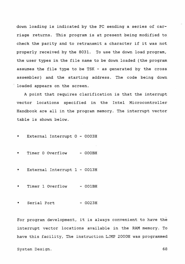
assumes the file type to be TSK - as generated by the cross

assembler) and the starting address. The code being down

loaded appears on the screen.

A point that requires clarification is that the interrupt

vector locations specified in the Intel Microcontroller

Handbook are all in the program memory. The interrupt vector

table is shown below.

• External Interrupt O - 0003H

• Timer O Overflow - OOOBH

• External Interrupt 1 - 0013H

• Timer 1 Overflow - OOlBH

• Serial Port - 0023H

For program development, it is always convenient to have the

interrupt vector locations available in the RAM memory. To

have this facility, The instruction LJMP 2000H was programmed

System Design. 68

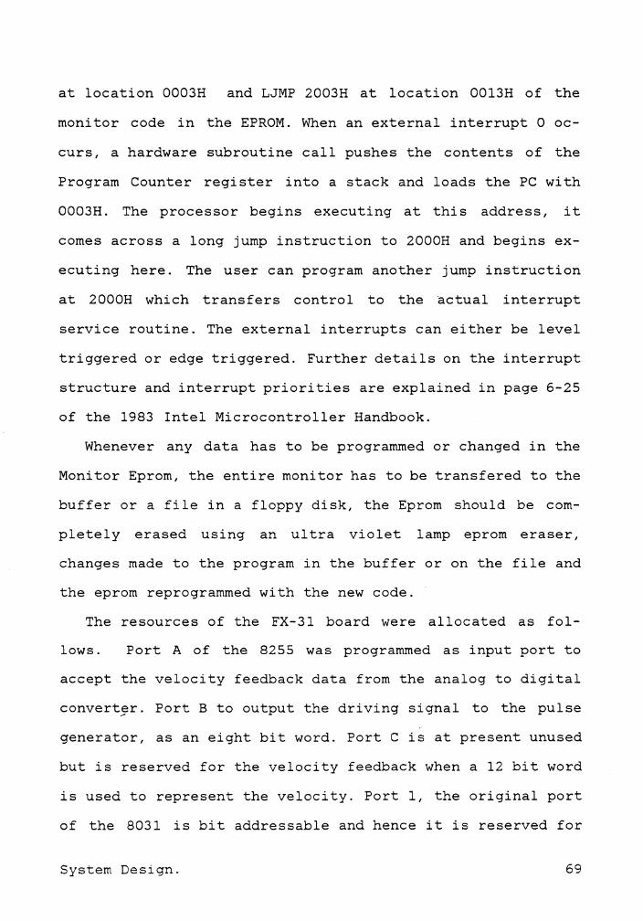
at location 0003H and LJMP 2003H at location 0013H of the

monitor code in the EPROM. When an external interrupt O oc-

curs, a hardware subroutine call pushes the contents of the

Program Counter register into a stack and loads the PC with

0003H. The processor begins executing at this address, it

comes across a long jump instruction to 2000H and begins ex-

ecuting here. The user can program another jump instruction

at 2000H which transfers control to the actual interrupt

service routine. The external interrupts can either be level

triggered or edge triggered. Further details on the interrupt

structure and interrupt priorities are explained in page 6-25

of the 1983 Intel Microcontroller Handbook.

Whenever any data has to be programmed or changed in the

Monitor Eprom, the entire monitor has to be transfered to the

buffer or a file in a floppy disk, the Eprom should be com-

pletely erased using an ultra violet lamp eprom eraser,

changes made to the program in the buffer or on the file and

the eprom reprogrammed with the new code.

The resources of the FX-31 board were allocated as fol-

lows. Port A of the 8255 was programmed as input port to

accept the velocity feedback data from the analog to digital

convert~r. Port B to output the driving signal to the pulse

generator, as an eight bit word. Port C is at present unused

but is reserved for the velocity feedback when a 12 bit word

is used to represent the velocity. Port 1, the original port

of the 8031 is bit addressable and hence it is reserved for

System Design. 69

control of the A/D converter and any other interface hardware

or peripheral to be added at a later date. INTO and INTl,

the external interrupt lines are used for position decoding.

The serial port, as mentioned earlier is the communication

link between the executive level and the higher levels of the

control hierarchy.

4.3.1 POSITION DECODING.

Position feedback data is available from each joint of the

manipulator arm. The position encoders are of the incremental

type [3] which produce 500 pulses per revolution of the motor

shaft. The incremental shaft encoder operates by translating

the rotation of the shaft into interruptions of a light

beam which are then output as electrical pulses. The standard

"Code Wheel" is a metal disc which has 500 equally spaced

apertures around its circumference. A matching pattern of

apertures is positioned ..._ on a stationary phase plate adj a-

cent to the Code Wheel. A light beam will be transmitted

through the apertures only when the apertures in the code

wheel and the phase plate line up; therefore during one ro-

tation of the shaft, there will be 500 alternating light and

dark periods. Photo diodes detect these light beams and

conVert it to an electric pulse. The light sources are light

emiit:ing diodes. The apertures for each pair of photo diodes

that. form a 'channel' are placed so that a light period on

System Design. 70

one corresponds to a dark period on the other. The distance

between apertures of the two 'channels' are such that there

is a 90 degree phase shift between the pulses from each

channel. An optional 'index channel' is the third. Index

pulse of typically 1 cycle width is generated for each rota-

tion of the code wheel. This channel is not used for position

decoding in the development system. Figure 18 on page 72

shows the different pulses generated by each incremental en-

coder as well as the decoding circuitry.

Channels A and Bat TTL level are derived by using an op-

tical isolator followed by a inverter gate. The pull up re-

sistor on the collector of the opto isolator transistor was

experimentally chosen so that the TTL pulse from the inverter

would have 50% duty cycle. The problem of decoding the di-

rection of rotation of the shaft, from these signals has an

interesting solution [ 19]. Figure 19 on page 73 shows the

four unique states of the encoder and the unique sequences

of possible encoder outputs for continuous motion in each

direction.

The goal was to get a "Count Up" pulse when the shaft rotated

in one direction and a "Count Down" pulse in the other di-

rection. An eprom was used in a feed back structure so that

it works as a finite state machine. Only four address lines

and four data lines are used. The remaining address lines are

grounded and the data lines left floating. These four ad-

dress lines can address sixteen memory locations and the data

System Design. 71

{/)

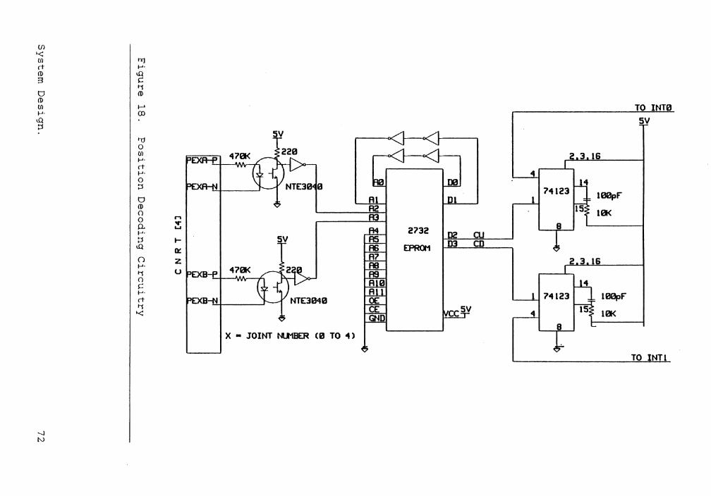
'< Ul rt (1) 3 t:J (1) Ul I-'·

I.Q ::1

--.J N

h:J I-'· I.Q s:: l"1 (1)

I-' 00

trj 0 Ul I-'· rt I-'· 0 ::1 t:J (1) 0 0 p. I-'· ::1

I.Q

0 I-'· l"1 0 s:: I-'· rt l"1 '<

5V

M .. .., .... 5V O! z u

X • JOINT Nlt1BER (0 TO 4)

TO INT0 5V

4 D0

l00pf"

101<

2732 OJ EPRCX1 CD

l 74123 l00pf"

101<

TO NTl

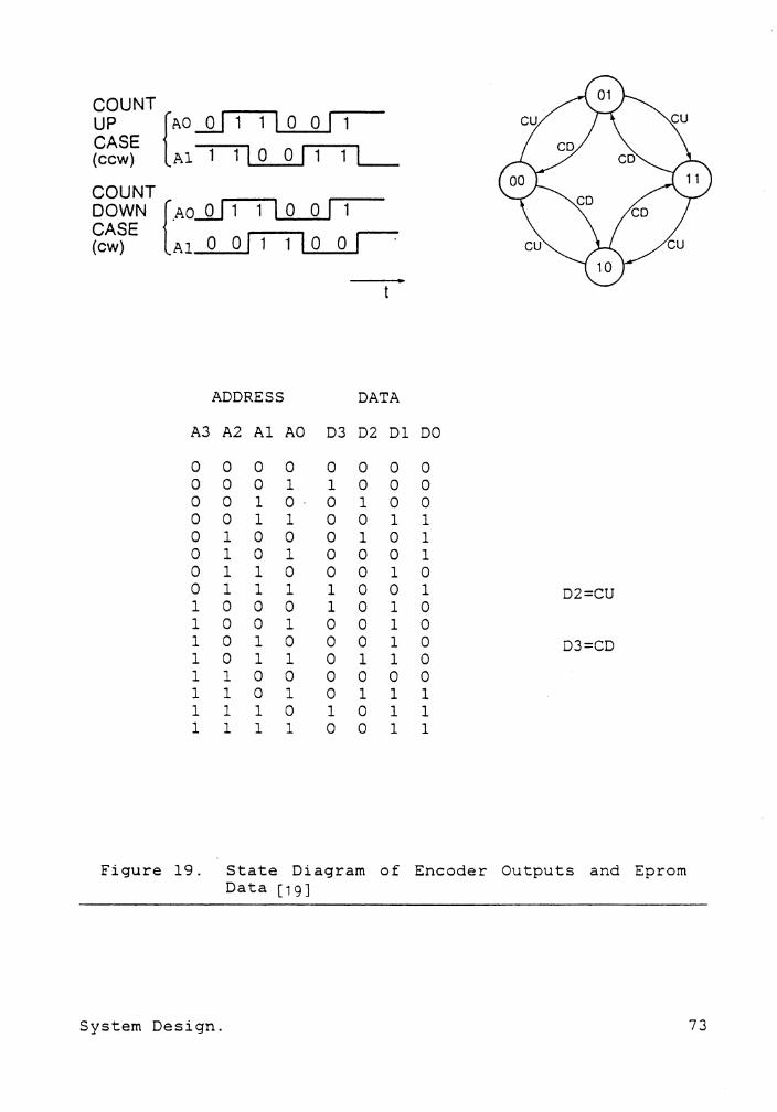
COUNT UP {P..0 _.Q.J 1 1 ! 0 0 ! 1 CASE (ccw) Al 1 1 I O O I 1 1 L_ COUNT DOWN {·Ao.JU 1 1 I o o I 1 CASE (cw) Al O O l 1 1 ! 0 0 !'

ADDRESS DATA

A3 A2 Al AO D3 D2 Dl

0 0 0 0 0 0 0 0 0 0 1 1 0 0 0 0 1 O· 0 1 0 0 0 1 1 0 0 1 0 1 0 0 0 1 0 0 1 0 1 0 0 0 0 1 1 0 0 0 1 0 1 1 1 1 0 0 1 0 0 0 1 0 1 1 0 0 1 0 0 1 1 0 1 0 0 0 1 1 0 1 1 0 1 1 1 1 0 0 0 0 0 1 1 0 1 0 1 1 1 1 1 0 1 0 1 1 1 1 1 0 0 1

DO

0 0 0 1 1 1 0 1 D2=CU 0 0 0 D3=CD 0 0 1 1 1

Figure 19. State Diagram of Encoder Outputs and Eprom Data [19]

System Design. 73

from the table in Figure 19 on page 73 is used to program

these locations. Address lines A2 and A3 receive the condi-

tioned signals from the encoder. Data lines D2 and D3 output

the "Count Down" and "Count Up" signals. DO and Dl are fed

back to AO and Al through a delay (two inverter gates in se-

ries).

The operation of the circuit is as follows. Consider the

inputs A2=1, A3=0 and assume the output to be 0010. Since the

lower two bits of the output form the lower bits of the ad-

dress, the effective address is 1010 and the data lines will

carry its contents - 0010. This represents a stable state

as AO / DO · and Al / Dl have the same value. Now, if A2

changes from O to 1, the input address becomes 1110. Data

lines will carry 1011 ( as per the table). After the delay

caused by the inverters in the feedback circuit, AO and Al

will be forced to the 11 state, changing the -input address

to 1111. Again a look up is done and the data corresponding

to this address - 0011 is output. This is again a stable

state. What actually transpired when A2A3 changed from 10

to 11 is that a pulse ( duration equal to the delay in the

feedback circuit) appeared on the "Count Down" line! Simi-

larly, if A2 now becomes 0, a pulse will appear on the "Count

Up" line. The table of data for the eprom is so devised that

if some malfunction occurs and A2A3 transits directly from

00 to 11 or from 01 to 10, no pulse will be generated by the

eprom.

System Design. 74

The position of each joint is to be kept track of, as a

count of the pulses from the encoder. The Count Up and Count

Down lines are connected to the INTO and INTl external in-

terrupt pins of the 8031. When a Count Up pulse occurs, the

interrupt service routine associated with interrupt O incre-

ments contents of a memory location in the FX-31 RAM desig-

nated as POSCOUNT. If a Count Down occurs, the contents of

POSCOUNT is decremented. POSCOUNT is a 16 bit word or double

byte. The disadvantage with this system is that when the

joint is moving with high speed, a large number of interrupts

will be generated, leaving the processor much less time to

do other computation. At its highest speed, one interrupt

will be generated every 30 micro seconds. Although the arm

will rarely be moved at its highest speed, this problem could

be alleviated, at the expense of accuracy, by placing flip-

flops (divide by 2) between the interrupt pins and the count

up/ count down lines.

A short program in 8031 assembly language is included in

the appendix. This will serve as the interrupt service rou-

tine and show how the interrupts are enabled and their modes

selected.

4.3.2 VELOCITY FEEDBACK.

The velocity or the derivative feedback is obtained from

the tachogenerators attached to each actuator. They are rated

System Design. 75

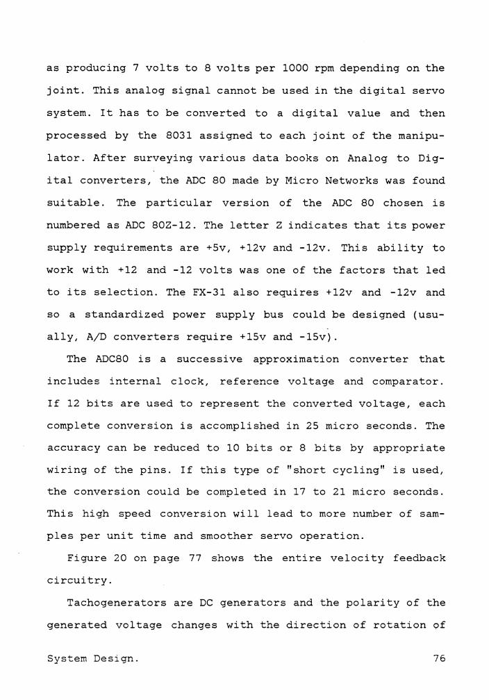
as producing 7 volts to 8 volts per 1000 rpm depending on the

joint. This analog signal cannot be used in the digital servo

system. It has to be converted to a digital value and then

processed by the 8031 assigned to each joint of the manipu-

lator. After surveying various data books on Analog to Dig-

ital converters, the ADC 80 made by Micro Networks was found

suitable. The particular version of the ADC 80 chosen is

numbered as ADC 802-12. The letter Z indicates that its power

supply requirements are +Sv, +12v and -12v. This ability to

work with +12 and -12 vol ts was one of the factors that led

to its selection. The FX-31 also requires +12v and -12v and

so a standardized power supply bus could be designed (usu-

ally, A/D converters require +lSv and -15v).

The ADC80 is a successive approximation converter that

includes internal clock, reference voltage and comparator.

If 12 bits are used to represent the converted voltage, each

complete conversion is accomplished in 25 micro seconds. The

accuracy can be reduced to 10 bits or 8 bits by appropriate

wiring of the pins. If this type of "short cycling" is used,

the conversion could be completed in 17 to 21 micro seconds.

This high speed conversion will lead to more number of sam-

ples per unit time and smoother servo operation.

Figure 20 on page 77 shows the entire velocity feedback

circuitry.

Tachogenerators are DC generators and the polarity of the

generated voltage changes with the direction of rotation of

System Design. 76

[/}

'< en trJ rt ...... Cl) '§ :3 t:1

11 (1)

(I) en N ...... 0 <Q ::,

<: (I) I-' 0 Cl ...... rt '< TG X A trJ (I)

.. N

(I)

Ill Cl

~:z l' lH .

I- lM ;,;' z 0 u ...... ' 11 Cl TG X B r:: ...... X•JOINT NO.C0 TO 4> rt

-..J -..J

-12V +12V

12 15 21

lH 30

I" 17

r 25 V 13

TL081 5V ...; :..

lH 101< .. 19

+l2V & -12V F'OR OP RP 20 9 7

31 32

l 2 3

N -,!, 4 IS) 5 m

6 16

10 15

22 18

I

LSB

HSB

==

0

..

a:

.0 luF'

C ONVERT ROM Pl.0 ~,

t. . 0 . C TO Pl.l

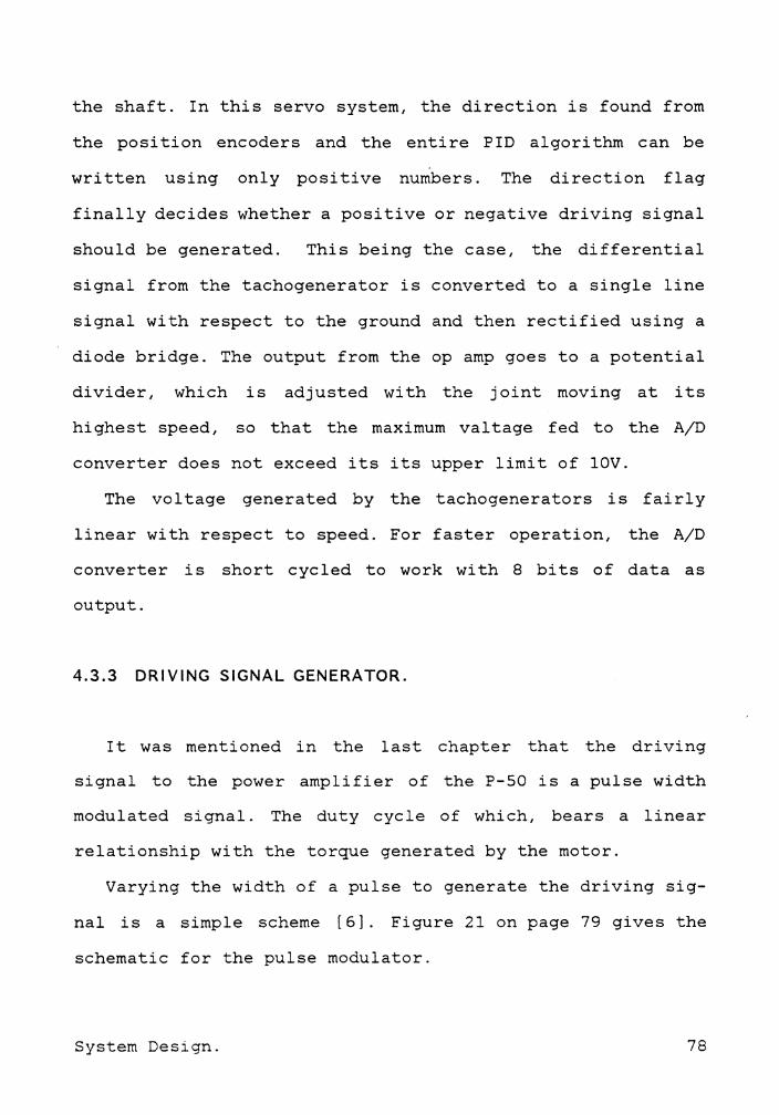
the shaft. In this servo system, the direction is found from

the position encoders and the entire PID algorithm can be

written using only positive numbers. The direction flag

finally decides whether a positive or negative driving signal

should be generated. This being the case, the differential

signal from the tachogenerator is converted to a single line

signal with respect to the ground and then rectified using a

diode bridge. The output from the op amp goes to a potential

divider, which is adjusted with the joint moving at its

highest speed, so that the maximum val tage fed to the A/D

converter does not exceed its its upper limit of lOV.

The voltage generated by the tachogenerators is fairly

linear with respect to speed. For faster operation, the A/D

converter is short cycled to work with 8 bi ts of data as

output.

4.3.3 DRIVING SIGNAL GENERATOR.

It was mentioned in the last chapter that the driving

signal to the power amplifier of the P-50 is a pulse width

modulated signal. The duty cycle of which, bears a linear

relationship with the torque generated by the motor.

Varying the width of a pulse to generate the driving sig-

nal is a simple scheme [ 6]. Figure 21 on page 79 gives the

schematic for the pulse modulator.

System Design. 78

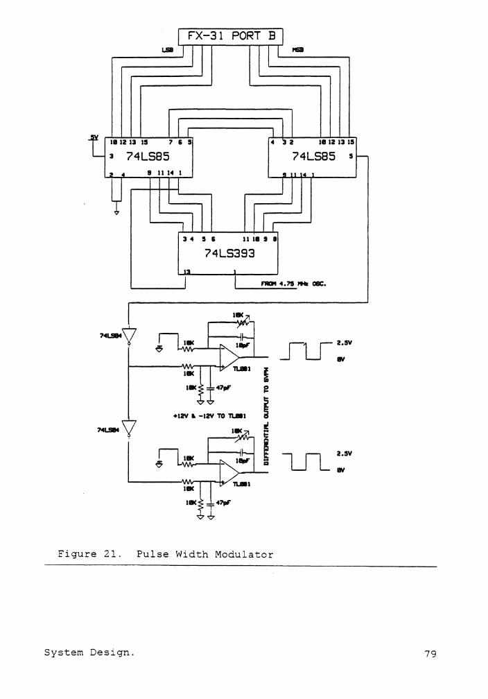
FX-31 PORT B I LSB

I I 1611

I I I t 181213 15 7 6 S 4 '3 2 18 12 13 IS

3 74LS85 74LS85 s ,-

1 • 9 II 14 I !I , • ,

I 741.S14y

741.S14

I

I I I 34 5 g II 18 9 8

74LS393 1:1 I

I I

I~.}'!_ --·

+l2V • -l2V TO n.m1

Ill<

F'ID'I 4. ,s ... O&C.

7 n a.sv LJ L"'

Figure 21. Pulse Width Modulator

System Design. 79

?4LS04

------ D 1-------1---.

4.75 MHz XTRL

0.00iul=""

Figure 22. Crystal Oscillator

4?0pF

System Design. 80

The signal output from the FX-31 board is an eight bit word.

If the word is OOH, then the duty cycle of the generated pulse

must be zero and the motor will give maximum torque in the

negative direction. If the word is 7FH, the duty cycle of the

pulse is 50% and the motor is in hold. A FFH would lead to

100% duty cycle and maximum torque in the positive direction.

To generate a pulse stream, a crystal oscillator oscil-

lating at 4.75MHz is used (Figure 22 on page 80). This is a

simple oscillator made of inverter gates and was found to

work very well. The output of the oscillator is fed to an

eight bit binary counter. The counter counts from OOH to FFH,

resets and begins the count again.

A digital magnitude comparator compares the count of the

counter and the 8 bit output from portB of the FX-31 at each

instance and indicates which input is higher. The logical

state of the line that indicates whether the counter is

higher than the set word is the actual pulse width modulated

signal. The frequency of this pulse is 18. 555kHz

( 4750kHz/256 = 18. 555kHz). The original controller uses a

pulse width modulated signal of 18.658kHz but the difference

does not matter.

4.4 THE MASTER CONTROLLER.

The master controller or the strategical/tactical level,

is basically software, written in some high level language

System Design. 81

like Fortran and operates on the IBM PC. The PC has two disk

drives and 256K of RAM on the mother board. An additional

384K bytes of RAM was added expanding the total memory to

640K. This memory expansion board (AST 6 PAK PLUS from AST

Research Inc.) has also got a real time clock as well as a

serial port and a parallel printer port. No problem was

faced in installing this board. However, when the serial

port was hooked up to the local net, it was found necessary

to force the CTS, DSR and DCD lines high before the terminal

emulation software (YTERM) could work. To make these pins a

logical high, each jumper pin on the block associated with

the serial port has to be shifted one pin to the right. This

particular serial port is configured as C0Ml (port 3F8H on

the PC) and was assigned solely for communication with higher

levels on main frame computers through the local net.

An 8087 math coprocessor was installed in the IBM PC to

extend its computation capability. This was tested using di-

agnostic routines and found to work well. The Fortran com-

piler (Microsoft Fortran 3. 2) makes use of the 8087 and is

claimed to execute numerical problems up to ten times faster

than without the coprocessor.

Greg Sherman of the Mechanical Engineering Dept., wrote

the user interface software in different high level lan-

guages. Surprisingly, compiled BASIC was found to execute the

fastest and moreover, the input/ output commands of the IBM

PC BASIC are tailored for the machine. In certain instances

System Design. 82

for better control of the CRT screen, routines were written

in 8086 assembly language and linked to the BASIC program.

This level presents the user with various options and sub-

options. The user will be able to change all the control

constants of the servo as well as display the position and

velocity feedback from each joint, on the screen.

To move the TCP of the robot (in the fully developed ver-

sion), the user can enter a serie.s of absolute coordinate

points through which it should move. The software that makes

up the strategical level then splits this job into different

moves. The tactical level (depending on how the control al-

gorithm is written) plans the trajectory of the TCP between

the end points of the move, and makes a table of the positions

of each joint with respect to time. When the robot is re-

quired to move, this table is looked up and data for each

joint is transmitted to the respective FX-31 board for exe-

cution of the movement. The time interval between consecutive

changes in these "set points" depend on the control algorithm

and actual timing could be done with the real time clock on

the AST SIX PAC board.

The communication between the IBM PC and the FX-31 boards

are through five individual serial lines. Serial communi-

cation was chosen to enhance the flexibility of the system.

This way, the IBM PC can be replaced with a more powerful

computer with no hardware changes. The reason for having five

separate serial lines instead of one running through all the

System Design. 83

boards was to lessen the number of interrupts on each

processor. If just one line was used, each time a message

appears on the line, all the processors will be interrupted

to check if that message is for them. Another main advantage

of having individual lines is that different joints could be

controlled by different computers if the need arises. Since

the communications routines in the monitor of the FX-31

boards are to be used, a simple communication protocol could

be developed from the commands already available in the mon-

itor.

The fully integrated Robot Control Development System

could be built using the guide lines in this chapter. Most

of the hardware for the servo was built and tested. What re-

mains is mainly the software for the strategic level, tac-

tical level, the PID controller and the communications. The

strategical and tactical level software will change with each

user, since the RDS is being built for testing the software

on an industrial grade robot.

System Design. 84

5.0 CONCLUSION.

The development system for the P-50 process robot, when

fully functional, will serve as the Robot Development System.

This controller was designed with maximum emphasis on flexi-

bility. The design represents the result of a study of vari-

ous, state of the art, control philosophies and the

hardware/software required to implement them in an industrial

robot.

To summarize the work done till the present: - The Robot

Control Development System is being designed and constructed

on the manipulator arm of the P-50 process robot. The choice

of this robot was entirely due to its availability for ex-

perimentation. The lack of circuit diagrams and other tech-

nical details about the controller of the P-50 proved to be

a major stumbling block. However after much probing and ex-

perimentation, techniques to disable the original controller

and transfer control to the development system were discov-

ered.

In the mean time, many control structures and ways of im-

plementing different control algorithms were studied. This

resulted in the conceptualization and design of a hierarchi-

cal control structure. The main components of this type of

structure are the executive level forming the lowest level

of the hierarchy, preceded by the tactical level, strategical

Conclusion. 85

level and the human interface level. This structure lends

so much flexibility to the controller that many other levels

can be incorporated depending on the need.

The advantages of sampled data control systems [ 11] like

improved sensitivity, better reliability, zero drift and high

flexibility weighed heavily in favor of an entirely digital

controller. Moreover, the high speed and performance of the

modern microprocessors make digital systems fast enough for

real time control purposes.

The hardware required for this project was chosen depend-

ing on the availability, cost and performance of each device.

An IBM PC with 640K bytes of RAM and an 8087 math coprocessor

became the master computer. Intel 8031 microcontrollers in

the form of single board computers (FX-31) were chosen to be

the slave units or the executive level that executed the ac-

tual motion of each joint.

Communication between the master computer and the slave

units are through three-wire serial lines. Five serial ports

were installed on the PC to provide individual lines to each

of the microcontrollers. The reasons for adopting such a

scheme are explained in Chapter 4.

It was decided to implement a PID controller as the servo

system in the executive level. Circuits were designed to

condition and interface the position / velocity feedback

signals to the micro controller. The analog voltage output

of the tachogenerators was found to be linear over most of

Conclusion. 86

its operating range and it is considered to be linear over

the entire range for easier computational purposes.

The PID controller on the 8031 boards receive the set

point or the reference position from the IBM PC through the

serial port. The output from the micro controller is an eight

bit word. Driving signal to the power amplifier of the P-50

is a pulse train. A pulse width modulator was designed and

built. The digital output of the PID controller is used to

modulate the duty cycle of the pulse train. There is a linear

relationship between the duty cycle of this pulse train and

the torque output of the motors.

5.1 MODIFICATIONS TO THE SYSTEM.

One area that might require refinement, is the way posi-

tion information is up dated. Currently, external interrupts

are generated for every pulse of the incremental position

encoders. This could lead to a large number of interrupts,

in extreme cases, that will prevent the processor from exe-

cuting its normal tasks of running the PID control algorithm.

At the expense of sacrificing accuracy, the pulses from the

decoding circuits could be divided by a factor of two, to

reduce the number of interrupts. In this case, the resolution

of the encoder will drop from 500 pulses per revolution to

250 pulses per revolution. Another way of overcoming this

problem is to have a counter external to the microcontroller

Conclusion. 87

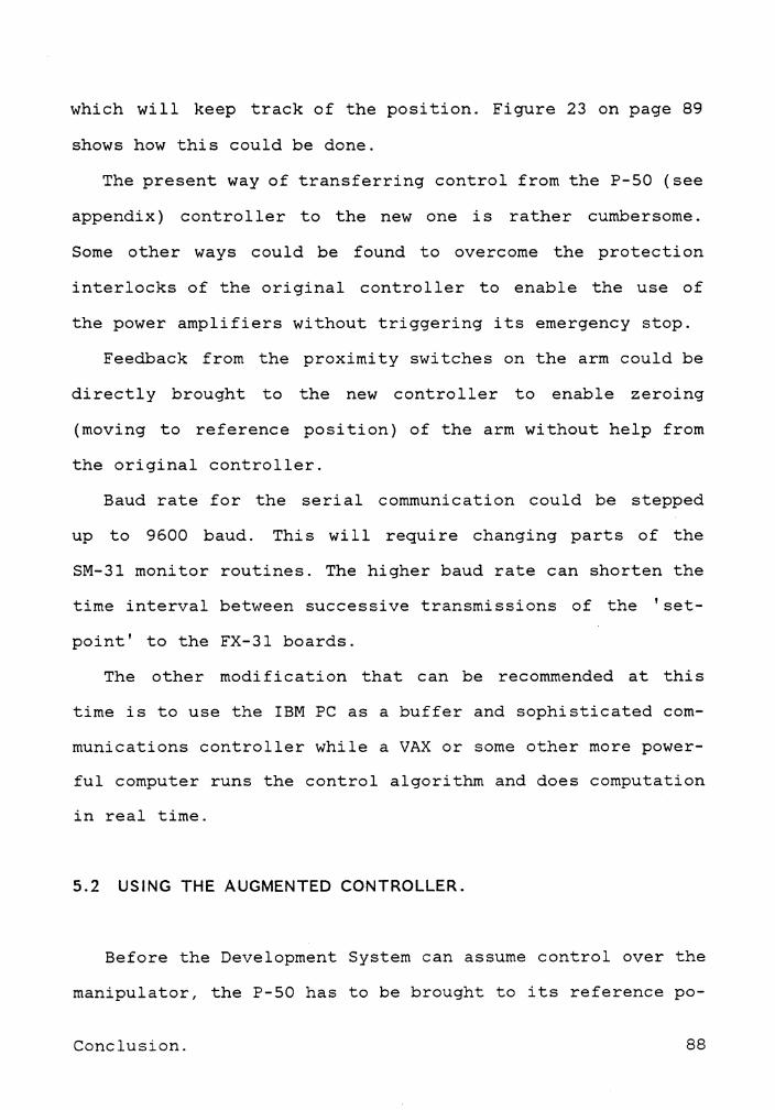
which will keep track of the position. Figure 23 on page 89

shows how this could be done.

The present way of transferring control from the P-50 (see

appendix) controller to the new one is rather cumbersome.

Some other ways could be found to overcome the protection

interlocks of the original controller to enable the use of

the power amplifiers without triggering its emergency stop.

Feedback from the proximity switches on the arm could be

directly brought to the new controller to enable zeroing

(moving to reference position) of the arm without help from

the original controller.

Baud rate for the serial communication could be stepped

up to 9600 baud. This will require changing parts of the

SM-31 monitor routines. The higher baud rate can shorten the

time interval between successive transmissions of the 'set-

point' to the FX-31 boards.

The other modification that can be recommended at this

time is to use the IBM PC as a buffer and sophisticated com-

munications controller while a VAX or some other more power-

ful computer runs the control algorithm and does computation

in real time.

5.2 USING THE AUGMENTED CONTROLLER.

Before the Development System can assume control over the

manipulator, the P-50 has to be brought to its reference po-

Conclusion. 88

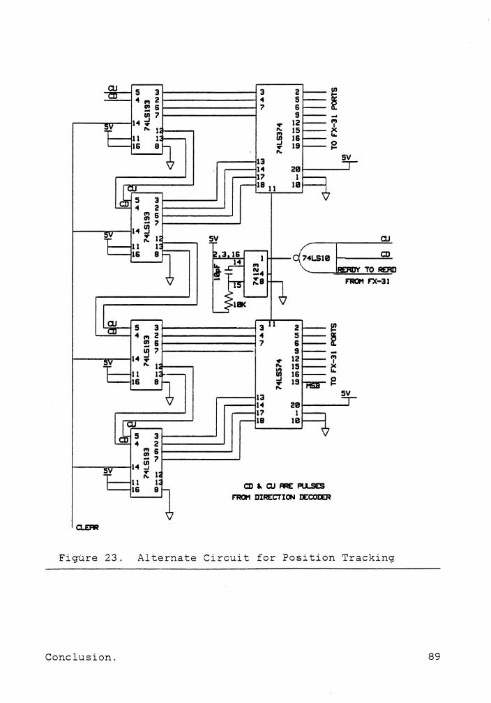
QJ

5V

~ir--t5 3--------~ OI 6 1----------t

? "' la----,

1 8

31--------' 2------' 1"161-------!!? ? 1---------'

1-----.. ......

3

?

2 i 5 6 9 -12 l"I y

"' 15 16

y 19 "' 5V

2B 1

1B

QJ

,;,:LSIB E CD TO READ

2 5 6 9

t 12 l:t 15 :l 16 y 19 "'

F'R0t1 F'X-31

l l 1 8 CD a. QJ PAE PU.SES

F'R0t1 DIRECTION IECOIER

Figure 23. Alternate Circuit for Position Tracking

Conclusion. 89

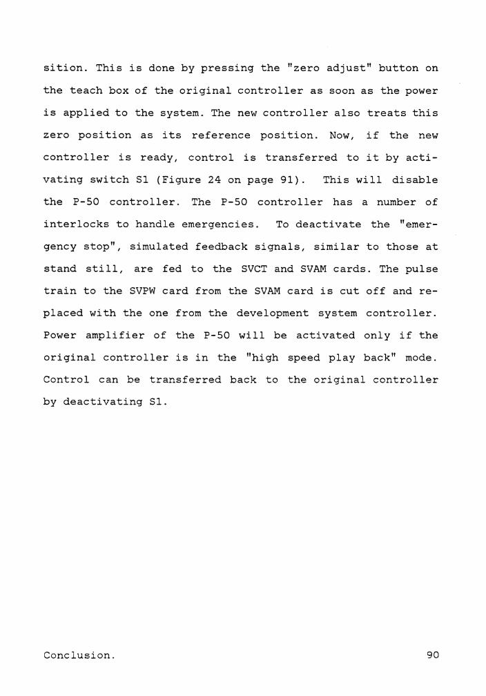
sition. This is done by pressing the "zero adjust" button on

the teach box of the original controller as soon as the power

is applied to the system. The new controller also treats this

zero position as its reference position. Now, if the new

controller is ready, control is transferred to it by acti-

vating switch S1 (Figure 24 on page 91). This will disable

the P-50 controller. The P-50 controller has a number of

interlocks to handle emergencies. To deactivate the "emer-

gency stop", simulated feedback signals, similar to those at

stand still, are fed to the SVCT and SVAM cards. The pulse

train to the SVPW card from the SVAM card is cut off and re-

placed with the one from the development system controller.

Power amplifier of the P-50 will be activated only if the

original controller is in the "high speed play back" mode.

Control can be transferred back to the original controller

by deactivating Sl.

Conclusion. 90

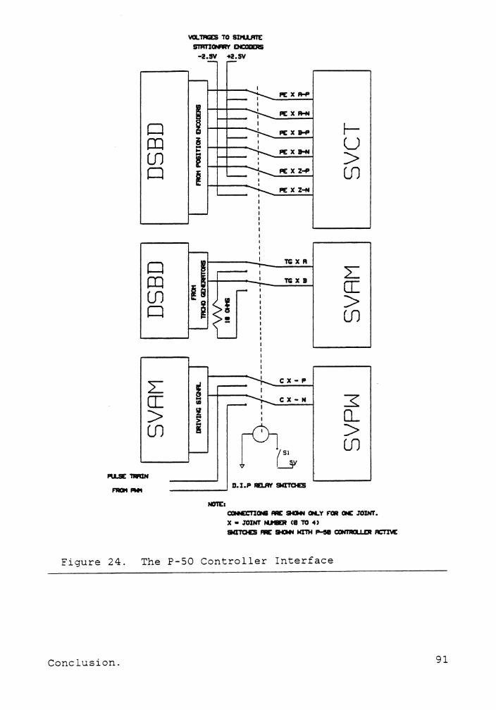
D CD lf1 D

Cl CD lf1 D

2:: er: > lf1

PU.SE'TIIIUN

FR0II .....

\la.TAGIES TO SDUJffE STRnCNR'I ENC0DER5

-2.IV +2.IV

I § .. ... ! I

-i ... .. -I

PE X A-fl

PE X 11-H

PE X &-49

PEX ...

PE X Z~

PE X

TG X A

TG XI

cx-P

CX-N

!i 0~ -___ __. D.I.P IIELIW SIGTO£S

Nln'Ea

r-u > lf1

2:: er: > lf1

Q_ > lf1

CIHETICNI flE SNMI CN.Y F'CII QC JODff. x • JOJNI' JU&R ca TO 4> aaTO£S .. 90N NI1H ..... c:cNTA0LL£R ACTnE

Figure 24. The P-50 Controller Interface

Conclusion. 91

This thesis presents the preliminary work done in concep-

tualizing and designing the hardware for the new P-5O con-

troller. One servo unit was constructed and tested to

validate the design. It was found to work well. The software

for the entire controller remains to be written. Once this

is done according to the design specified in this thesis, the

user of the system will be able to program motion of the tool

center point of the manipulator by specifying the coordinates

of the points through which it is supposed to move. The user

will also be able to change the constants of the servo system

and restructure the entire control scheme through software.

The position and velocity of each joint at any instance could

also be displayed on the CRT terminal to enhance the testing

and validation of complex control algorithms. The completed

system can be used to conduct research in other fields such

as human factors engineering (man-machine interface schemes),

kinematic and dynamic studies.

Conclusion. 92

APPENDIX A. ANALOG TO DIGITAL CONVERTER SPECIFICATIONS.

When connecting the A/D converter in the velocity feedback

circuit, proper attention to layout and decoupling is neces-

sary to ensure accuracy of the converted data. Analog and

Digital Ground pins are not connected internally, they should

be tied together to a large analog ground. plane under the

chip. Coupling between the analog inputs and digital signals

should be minimized to avoid noise pickup. Power supplies

should be decoupled with tantalum or electrolytic capacitors

located close to the ADC80. For optimum performance, accord-

ing to the manufacturer, 1 micro farad capacitors paralleled

with 0.01 micro farad ceramic capacitors should be connected

as shown in the figure next page.

For normal operation a positive, 100 nano second wide,

input pulse is applied to the Convert Command input. The

rising edge of the convert command will start the internal

clock and initiate conversion. The Convert Command input must

remain low until the End of Conversion output returns low,

indicating the end of conversion period. The External Clock

and Clock Inhibit inputs must be tied high for normal opera-

tion.

Further information about the ADC80 is available in the

1984 Micro Networks (Division of Unitrode) catalog.

Appendix A. Analog to digital converter specifications. 93

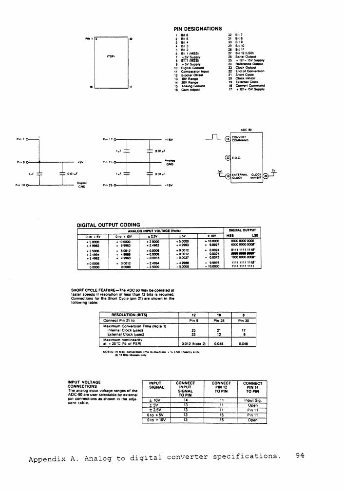
Pin 7

Pi" 9

Pin 100

l,1F

T

PIN DESIGNATIONS 8116 32 Bit 7

""'' . 811 5 31 8118 BIi, 30 Bit 9

• Bil 3 29 Bil 10 5 811 2 28 81111 6 8111 (MSB) 27 Bit 12 ILSB)

110,i 7 26 Se,1a1 Oulpul 8 25 - 12/ - 15V Supply 9 + SV Supply 2, Reference Oulpul

10 Otg11a1 Ground 23 Clock Oulpul 11 Comparator lnpul 22 End of Com,e,saon 12 21 Shon Cycle 13 t0V Range 20 Clock lnh&bil 1, 20V Range 19 Exlemal Clock

ti 17 15 Anatog Ground 18 COnwtfl Command 18 Gain Ad1usl 17 + 12/ • 15V Supply

AOC 80

P,n 1701•, 1 CONVfRT I +ISV COMMAND

+SY ...... I f" GNO

001-,F

..... 100

'•' I oo1••-,sv T o, ..... P,n250 I EXTERNAL CLOCK 20 CLOCK INHIBIT

GNO

DIGITAL OUTPUT CODING ANALOG INPUT VOL TAQE (Yottal DIGITAL OUTl'UT

0 lo +SY Oto+ 10V s:2.5V •5Y • 10V MSB LSB

+ 5.0000 + 100000 +2.5000 +. 99112 9.9983 + 2.4912 + 25006 + 50012 +0.0008 + 2.4994 + ,.9988 -o.oooe + 2 4982 + • 9963 -0.0018

+0.0008 + 0.0012 -2.,994 0.0000 0.0000 -2.5000

SHORT CYCLE FEATURE-The ADC 80 may lie operaled at laster speeds If resolullon of leas lhan 12 bits Is required. Connec:llons for the Short Cycle (p,n 21) are snown In Ille follow1ng lable:

RESOLUTION (BITS) Connecl Pin 21 to Maximum Conve,slon Time (Nole 1)

Internal Clock <,.sec) External Clock ~,sec)

Maximum nonhneanty

+ 5.0000 10.0000 .,.9983 + 9.11927 +0.0012 + 0.0024 -0.0012 - 0.002, -0.0037 - 0.0073 -·- - 9.9978 -5.0000 - 10.0000

12 10 Ptn 9 Pin 28

25 21 23 12

al + 25 •c (¾ ol FSR) 0.012 (Note 2) 0.048

NOTES IH Me•. conwetsM>n II~ 10 ma1nt .. n :t 'It LSB llnee,Uy eno,. 121 12 Bits MOOets only

INPUT VOLTAGE CONNECTIONS The analog input voltage ranges of the AOC-80 are user selectable by ex1ernal pm connections as shown in the adja-cent 1able.

INPUT SIGNAL

:t lOV + SV :!: 2.SV

Oto +SV Oto +10V

CONNECT INPUT

SIGNAL TOPIN

14 13 13 13 13

CONNECT PIN 12 TOPIN

11 11 11 15 1,

0000 0000 0000 0000 0000 ooo,• 01111111 ,,,,. ---· 1000 0000 ooo,· 11111111 ,,,,. 111111111111

a Pin 30

17 6

0.C..8

CONNECT PIN 14 TOPIN

lnpu1 Sig. Open Pin 11 Pin 11 Open

sv

Appendix A. Analog to digital converter specifications. 94

APPENDIX B. ISL SIMULATION OF THE SERVO SYSTEM.

This simulation and modelling of the PID controller for

each joint (with the arm stretched horizontally - worst case)

of the manipulator was done by Ashi t Gandhi and Jayaram

Sankar. The dimensions of all the links of the P-50 were

measured and the volumes and masses calculated. From this the

mass moments of inertia for the links were found, about the

axes fixed to the links. Figure 25 on page 97 shows the

control schematic for each kinematic link, driven by an

electric motor.

Modelling of a robot arm is a highly complex task. The

model used here is for illustrative purpose and does not

consider friction or gravitational effects on the coupled

system. The goal of this simulation was to find out the ap-

proximate magnitude of the constants.

The ISL (Interactive Simulation Language) package was used

to find the best values of the control parameters of each

joint. It must be noted that the moment of inertia about axis

of joint 1 depends on the orientation of joints 2 and 3; that

of joint 2 depends on joint 3. Optimum values of the control

constants (K, K., Kd and K) for an input of 0 =0.2 radians p 1 a r and 0 1 , 02 , 03 equal to 1.047, -0.5236, -0.5236 radians, re-

spectively. Their values are tabulated in the next page.

Appendix B. ISL Simulation of the servo system. 95

K Kd K. K p l. a

I Joint 1 29 2 78 50

Joint 2 900 20 500 200

Joint 3 900 30 700 200

Appendix B. ISL Simulation of the servo system. 96

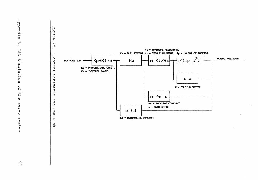
::i:, 'O 'O (1) ::s p_. I-'·

tp

H (/) t-1 (/) I-'· 3 C r' Ill rt I-'· 0 ::i

0 Mi

rt :::r (1)

en (1) ti <: 0

m '< m rt (D

3

I.O --..J

til I-'· IQ C ti (1)

N V1

0 0 ::i SET POSITIQ-1 rt ti 0 r'

(/) 0 :::r (1) 3 Ill rt I-'· 0

til 0 ti

0 ::i (1)

t-1 I-'· ::i

- Kp+Ki/s --l(p K

• ~TIClft.. CONST. I• lNTEGRFL CONST,

-

Ra • fRflTlR: RESISTRa Ka • Rt". FACTOR K\ • TORa..E CXINSTflrr Ip • t10t£NT CF Il€RTIR

Ka Kt/Ra --141 / C Ip s2) I R:TI..R.. POSITia-4 -- n I

C s

C • IRflNCi FACTOR

- n Ke s Ke • IRl< DF COHS1RlT n • CiEFR fffTIO

s Kd Kd IERIIIRTIVE COHS1RlT

APPENDIX C. SERIAL PORT CONFIGURATION·.

The serial port modules used for communications, are man-

ufactured by Maynard Electronics, Casselberry, Florida. These

modules use the 8250 UART (Universal Asynchronous Receiver/

Transmitter) which can be programmed for different baud rates

and has double buffering to eliminate need for synchroniza-

tion. These modules (maximum of six) plug into a "multi-

function card" which, in turn, plug into the expansion slots

on the IBM PC mother board.

The base address for each serial port module can be pro-

grammed by using shorting jumpers on the bank of connector

pins located on the edge of each module. Figure 26 on page

99 shows how this can be done.

It must be noted that the Eprom Programmer uses the port

address 0280H. The addresses recommended for use are under-

lined.

These serial ports are fully programmable and supports

asynchronous communications only. It can add and remove start

bits, stop bits, and parity bits. Baud rate can be programmed

for 50 to 9600 baud with five, six, seven or eight bit char-

acters [ 7].

Since the FX-31 serial port uses only pins 2, 3 and 7

(Transmitted Data, Received Data and Signal Ground), the in-

terrupts and modem control lines on these modules are not

Appendix C. Serial Port Configuration. 98

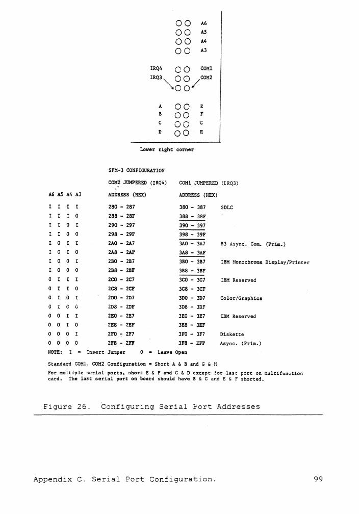
A6 AS A4 AJ

I I I I I I I 0 I I 0 I I I 0 0

I 0 I I I 0 I 0

00 A6

00 AS 00 A4 0 0 A3

IRQ4 Q O COMl IRQ3'\,_ 0 Q /COM2

'a00

A 00 E B 00 F C 00 ·G D oo H

Lower right corner

SPM-3 CONFIGURATION

COM2 JllMPERED (IRQ4)

ADDRESS (BEX)

COMl JUMPERED (IRQJ)

ADDRESS (HEX)

280 - 287 380 - 387 SDLC 288 - 28F 388 - 38F 290 - 297 390 - 397 298 - 29F 398 - 39F 2AO - 2A7 3AO - 3A7 BJ Async. Com. 2A8 - 2A1' 3A8 - JAF

(Prim.)

I 0 0 I 2BO - 2B7 3BO - 3B7 IBM Monochrome Display/Printer I 0 0 0 2B8 - 2BF 3B8 - 3BF 0 I I I 2CO - 2C7 3CO - JC7 IBM Reserved 0 I I 0 2C8 - 2CF 3C8 - 3CF 0 I 0 I 2D0 - 2D7 3D0 - 3D7 Color/Graphics 0 I C 0 2D8 - 2DF 3D8 - 3DF 0 0 I I 2EO - 2E7 3EO - 3!7 IBM Reserved 0 0 I 0 2E8 - 2EF 3E8 - 3EF 0 0 0 I 2FO-:- 2F7 3FO - 3F7 Diskette 0 0 0 0 2F8 :- 2FF 3F8 - EFF Async. (Prim.) NOTE: I - Insert Jwaper 0 - Leave Open

Standard COMl, COM2 Configuration• Short A & Band G & H For multiple serial ports, short E & F and C & D except for last port on multifunction card. The last serial port on board should have B & C and E & F shorted.

Figure 26. Configuring Serial ~ort Addresses


used. The section on IBM Asynchronous Communication Adapter

in [7] deals with serial ports and their programming. How-

ever, a concise description of how to initialize the ports

for 1200 baud, 7 data bits, 1 stop bit, one start bit and even

parity (SM-31 specifications), follows.

DLAB (Divisor Latch Access Bit) is bit 7 of the Line Con-

trol Register. The following registers are associated with

each serial port.

Port Address

Base Address+ 0

Base Address+ 0

Base Address+ 0

Base Address+ 1

Base Address+ 1

Base Address+ 2

Base Address+ 3

Base Address+ 4

Base Address+ 5

Base Address+ 6

Register

TX Buffer

RX Buffer

Divisor Latch LSB

Divisor Latch MSB

Interrupt Enable Reg.

Interrupt Identification

Line Control Register

Modem Control Register

Line Status Register

Modem Status Register

DLAB State

DLAB=O

DLAB=O

DLAB=l

DLAB=l

DLAB=O

XX

XX

XX

XX

XX

• Set DLAB=l by writing 80H into Line Control Register.

• To program baud rate for 1200 baud, OOH is written into

Divisor Latch MSB and 60H into Divisor Latch LSB.


• Reset DLAB and program the 8250 for even parity, 7 bit

word, and 1 stop bit by writing 3AH into Line Control

Register.

• Interrupts are disabled by setting all bits of Interrupt

Enable Register to 0.

The Line Status Register gives all the information regarding

the status of the port.

• Bit 0 when logical 1, indicates that an incoming charac-

ter has been received and transfered to the receive

buffer. It is reset when the processor reads the receive

buffer. By polling this bit, the processor will know when

to read the RX buffer.

• Bit 2 indicates parity error when set to logical 1.

• Bit 6 is the bit that shows the transmitter shift regis-

ter is empty. Any character for transmission must be sent

to the TX Buffer only when this bit is a logical 1. It

is reset upon a data transfer from the transmitter hold-

ing register to the shift register.

Information on the working of the 8031 serial port can be

found in the Intel Microcontroller Handbook [8].


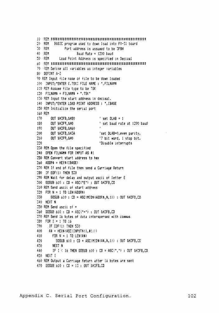
10 REM tttttttlttttttttttttttttttttttttttttttttttttttttt!ttt!t 20 REM BASIC progra~ used to da~n load into Fl-31 beard 30 REM Port address is assumed ta be 3F8H 40 RE:'! Baud Rate = 1200 baud 50 REM Load Point Address is specified in Decimal 60 REM ttttttttltSttltlttttttttttttttttttttttttttttttttttlttll 71) ?.EM Define all variables as integer variables 80 DEFINT A-Z 90 REM Input file name of file to be down loaded 100 IMPUT; 'EIHER (. TSKJ FILE NAME : ", FILNAMS 1!0 REM A~sute file type to be TSK 120 F!LNAM$ = FILNAMS • ".TSK" !30 RE~ Input the start address in decimal. 140 INPUT;"ENTER LOAD POINT ADDRESS: ',IBASE 150 REM Initialize the serial port 160 REM 170 OUT ~H3FB,~H80

OUT &H3F9,&HO 190 OUT &H3F8,&H60 200 OUT ~H3FB,&H3A 210 OUT ~H3F9,&HO 220 230 REM Open the file specified 240 OPEN F!LNAMS FOR INPUT AS 11 250 REM Convert start address to hex 260 ADDP.S = HEXS(IBASEJ

set DLAB = t set baud rate at 1200 baud

'set DLAB=O,even parity, '7 bit word, 1 stop bit. 'Disable interrupts

270 REN If end of file then send a Carriage Return 280 IF EOF(!l THEN 530 290 REN Wait for delay and output ascii of letter E 300 GOSUB 610 : CD = ASC ( • E • l : OUT &H3F8, CD 310 REM Send ascii of start address 320 FOR N = 1 TO LEN(ADDRSl 330 GOSUB 610 : CD= ASC!NIDS(ADDRS,M, ll l OUT ~H3FS,CD 340 flElT N 350 REN Send ascii of = 360 GOSUB 610 : CD= ASCl'="i : OUT &H3F8,CD 370 REM Send 16 bytes af data interspersed with commas 380 FOR I = t TO 16 390 IF EOF ! 1) THEN 530 400 Al= HEXS!ASCIINPUTSll,t!lll 410 FOR N = 1 TO LENIASI 420 50SUB 610: CD= ASC(NIDS(AS,N,111 : OUT &H3FB,CC 430 NEXT N 440 IF I< 16 THEN GOSUB 610: CD= ASC!',"l: OUT ~H3FS,CD 45(1 NEXT I 460 REM Output a Carriage Return after !6 bytes are sent 470 SOSUB 610: CD= 13 : &H3F8,CD


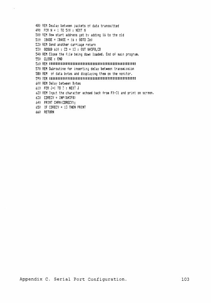
480 REM Dealay bebleen packets of data transmitted 490 FDR N = 1 TO 5(10 : tiEXT !l 500 REM New start address got by adding 16 to the old 510 !BASE= IBASE + !6: GOTO 260 520 REM Send another carriage return 530 GOSUB 610 : en= 13: OUT ~H3F8,CD 540 REM Close the file being down loaded. End of main program. 550 CLOSE: END 560 REM tt!tttttttttttttttttttttt!lttttitttttttttttttttttttt 570 REM Subroutine for inserting delay betNeen transmission 580 REM of data bytes and displaying them on the monitor. 590 REM tttttttttttttttttttt!tfttttttttttttttttttttttttttt!t 600 REM Delay between Bytes 610 FOR J=l TO:: NEXT J 620 REM Input the character echoed back from FX-31 and print on screen. 630 CDRECV = INP(~H3FBl 640 PR INT CHR$ ( CDRW/l ; 65(! IF CDRWJ = 13 THEN PRINT 660 RETURN


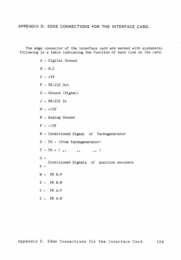
APPENDIX D. EDGE CONNECTIONS FOR THE INTERFACE CARD.

The edge connector of the interface card are marked with alphabets; following is a table indicating the function of each line on the card.

A - Digital Ground

B - N.C

C - +5V

F - RS-232 Out

G - Ground (Signal)

J - RS-232 In

M - +12V

N - Analog Ground

p - -12V

R - Conditioned Signal of Tachogenerator

S - TG - (from Tachogenerator)

T - TG + ( , , , , , , )

u -

V -Conditioned Signals of position encoders

W - PE B-P

X - PE B-N Y - - PE A_:P

Z - PE A-N

Appendix D. Edge Connections for the Interface Card. 104

APPENDIX E. FX-31 PIN CONNECTIONS.

22/44 Pin Connector SPecification

Pin for the 22/44 Pin connector is silkscreened on the component side of the board. With the board uPrisht and· the comPonent side showins, Pin 1 is on the left and Pin 22 on the

With th• board uPrisht and the solder side disPlaved < no silkscreen>, the Pin 23 is on the left and Pin 44 on the risht.

Pin# Function Pin# Function

1 +5V 23 GND0

2 N.C. 24 INTO 3 +12V 25 RD 4 PSEN 26 T1 5 -12v 27 TxD 6 ADO 28 A15 7 AD2 29 A13 • 8 AD4 30 A11 9 AD6 31 A9

10 AO 32 A7 11 A2 33 A5 12 A4 34 A3 13 A6 35 Al 14 A8 36 AD7 15 A10 37 AD5 16 A12 38 AD3 17 A14 39 AD1 18 RxD 40 -12v 19 TO 41 ALE• 20 WR 42 +12V 21 INT1 43 N.C. 22 ONO 44 +5V

40 Pin I/0 Connector Specification

Pin numberins for this connector is silkscreened on the board. Ports lines are abbreviated as shown on the schematic,

Pin•

1 2 3 4 5 6 7 8 9

10 11 12 13 14 15 16 17 18 19 20

Function

PA1 PA3 PA5 PA7 PC1 PC3 PCS PC7 +5V RS-232C TTL Out +5V PB1 PB3 PB5 PB7 Pl. 1 Pl.3 Pl.5 Pl. 7

Pin• Function

21 PAO 22 PA2 23 PA4 24 PA6

PCO 26 PC2 27 PC4 28 PC6 29 GND

Out 30 RS-232C 31 TTL In 32 GND 33 PBO 34 PB2 35 PB4 36 PB6 37 Pl.O 38 Pl.2 · 39 Pl.4 40 Pl.6 ·

Appendix E. FX-31 Pin Connections.

In

[ 1 ]

105

APPENDIX F. 8031 PROGRAMS.

The 8031 programs in the following pages were written to

test the hardware of the individual parts of the digital

servo system. Programs were edited using PCX editor on the

IBM PC, assembled using the 2500AD SOFTWARE INC. 8051 cross

assembler and down loaded into the FX-31 RAM.

The position encoding is tested by running the position

encoder testing program on the FX-31 board, with the IBM PC

configured as a dumb terminal (with Tech Term Software) and

linked to the micro controller board via the RS 232 lines.

When the robot arm is made to move, with the teach box, the

position count appearing on the terminal should increment or

decrement, depending on the direction of rotation of the

joint.

The velocity feedback is tested by applying a de voltage

between zero and ten vol ts, to the input of the A/D con-

verter. The digital equivalent of this analog signal should

appear on the terminal.

To test the pulse width modulator, an increasing count

(digital) is applied to the input of the PWM. The pulse width

of the pulse train from the PWM, seen on an oscilloscope

should vary from 0% to 100%.

Appendix F. 8031 Programs. 106

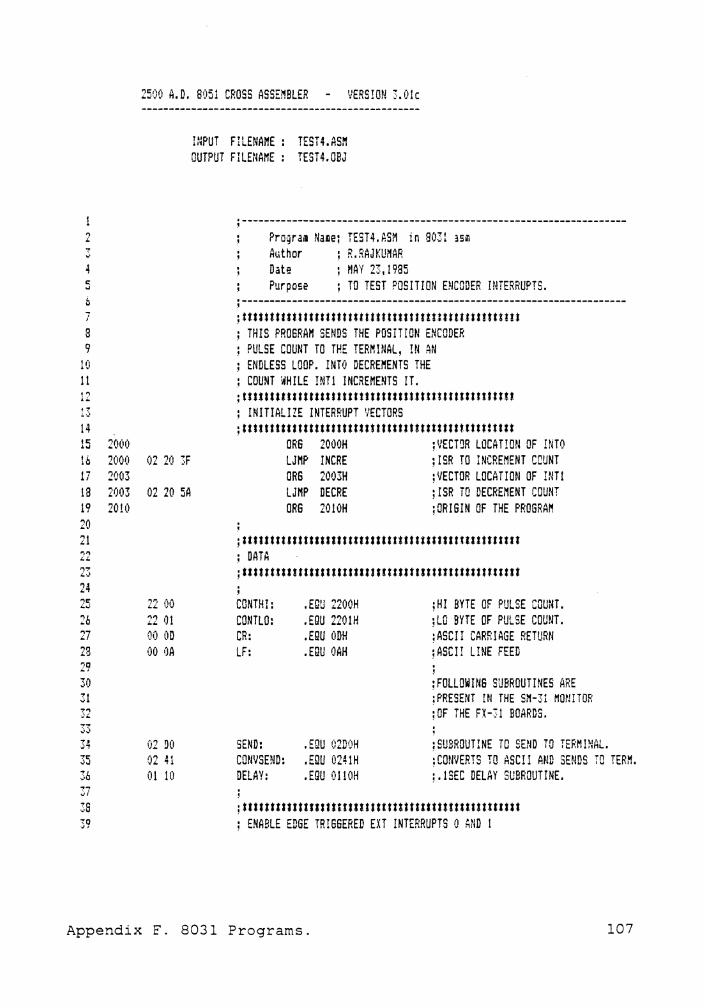
., i.. ,.

4 C: .., 6 ; I

3 9

1 (i 11 ,., ' .. ,.,.

14 15 20(H)

16 200(1 17 20(13 18 2003 19 2010 20 21 ,.,,, ..... ,.,.,. ;;..,.\

24 ,.,c: '-"' 26 27 .,!J •w 29 30 31 ~., .. , ... .,..,. .,;,,~

34 "'.'r ..)..!

36 ~"7 ..,, 39 39

2500 A.D. 8051 CROSS ASSEMBLER - VERSION 3.0lc

02 zrj 3F

02 20 5A

22 OIJ .,., ,Jl ...... DO OD 00 QA

02 DO 02 41 01 I (l

INPUT FILENAME: TEST4.ASM OUTPUT FILENAME: TESH.OBJ

·---------------------------------------------------------------------!

Prograa Name; TEST4.ASM in 8031 35~ Author R.RAJKUMAR Date MAY 23, 1985 Purpose TO TEST POSITION ENCODER INTERRUPTS .

·---------------------------------------------------------------------' ;tttttttttltttttttttt,ltttttttttttttttttt!tt!ttt!!t THIS PROSRAH SENDS THE POSITION ENCODER

; PULSE COU~H TO THE TEF:MHlAL, IN AN ; ENDLESS LOOP. INTO DECREMENTS THE ; COUNT WHILE INTI INCREMENTS IT. :ttttttttltttStttttttttttttttttttttttttttttttttttt ; INITIAL! ZE INTERRUPT \'ECTORS ;ttttttttttttttttttttttttttttttttttttttttttttttttt

ORS 2000H ;VECTQR LOCAT!ml OF HiTO LJMP INCRE ;ISR TO INCREMENT CCUNT ORS 2003H ; I/ECTOR LOCATION OF INT! LJMP DECRE ; ISR TO DECREMENT COUNT ORS 2010H ;ORIGIN OF THE PROGRA~

;ttttttttfttttttttttttttttttttttttttttttttltttltttl : DATA ;tttttttlttttttttttttttttt!ttttttSttttttttttttttttt

CONTHI: CONTLO: CR: LF:

SEND: COliVSEND: DELAY:

,EQU 2200H .mu 2201H .EQU ODH .mu rJAH

.EQU 02DOH

.EQU 0241H

.rnu 01 !0H

;HI BYTE OF PULSE COUNT. ;LG BYTE OF PULSE COUNT. ;ASCII CARRIAGE RETURN ;ASCII LINE FEED

; FOLLOW ms SUBR!lUTI NES ARE ; PRESENT IN THE SN-31 MONITOR ;OF THE FX-31 BOARDS.

: SUBROUTINE TD SEND TO TERM! NAL. ;CONVERTS TO ASCII AND SENDS TO TERM. ;.!SEC DELAY SUBROUTINE.

;tttttttlttttllttttttttttttttttttttttt!tttt!tlttttt ; ENABLE EDGE TRIGGERED EXT INTERRUPTS O AND I


42 201C D2 88 43 2012 D2 A8 44 2014 02 8A 45 2016 02 AA 46 47 48 49 50 c:, "'

54 55

2018 201B 20!C

90 22 00 E(!

12 (!2 41

56 20 !F A3 57 2020 EO 58 2021 12 02 41 59 60 2024 61 2026 62 2029 63 202B 64 65 202E 66 2031 67 2034 68 2037 69 2•)3A 70 203D 71 72 1'"'.! I._,

74 75

74 OD 12 02 DC 74 OA 12 02 DO

12 01 10 12 01 10 12 01 10 12 01 10 12 01 1 (! 01 18

76 203F CO DO 77 2041 CO EO 78 2043 C2 AS 79 2045 C2 AA so 81 2(!47 90 22 01 82 204A EO 83 204B 24 01 84 2040 FO 85 204E 50 24 86 2050 90 22 00 87 2053 EO

BE6IN: SETB ITO SETB EXO SETB IT! SETB EX!

;INTO TRANSITION ACTIVATED ; INTO ENABLED ;INTl TRANSITION ACTIVATED ; INT 1 ENABLED

;ttlttlttt!tttttttttltttt!tt!tttttttttttttttttt!ttl ; KEEP SENDING COUNT DATA TO SCREEN ;ttttttttttttttttttttttttlttttttt!!tttt!t!tt!!!tt!l

START: MOV OPTR,tCDNTHI ;CONVERT THE CONTENTS OF MOVI A,iDPTR ;CONTHI TO ASCII AND L CALL CONVSEND : SEND TO TERM HJAL.

INC DPTR MOVX A,~DPTR LCALL CONVSEND

MOV A,#CR LCALL SEND MOV A,ILF LCALL SEND

LCALL DELAY LC/ILL DELAY LCALL DELAY LCALL DELAY LCALL DELAY JMP START

;CONVERT CONTENTS OF ;CONTLO TO ASCII AND ;SEND TO TERMINAL.

;SEND CR&LF.

:.1 SEC DELAY

; LOOP BACK TO START.

:ttttttttttttttttttlttttttttttttt!ltttttttttttttttt , INTERRUPT SERVICE ROUTINES ;ttt!tttttttttttttttittttttttitttttttttrtttttttttst

INCRE: PUSH PSW PUSH A CLR E!O CLR EX 1

MOV DPTR,iCONTLO 110\IX A,ilDPTR ADD A,#01H MOVX aDPTR, A JNC BOBAK MOV DPTR,ICONTHI MOVX A,iDPTR

; SAVE PS\!! ON STACr-: ;SA\/E ACCUMULATOR ;DISABLE INTO :DISABLE INTl

; INCREMENT THE LO BYTE ;OF THE POSITION ;COUtHEF:. ;IF NO OVERFLOW, THEN RETURN. ; !F OVERFLOW, THEN : INCREMENT HI BYTE.


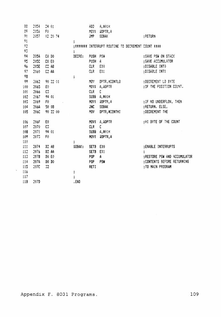
BB 2054 24 ()! ADD A,101H 89 2056 FO MOVX iDPTR,A 9(! 2057 02 20 74 Jl'!P GOBAK ;RETURN 91 92 ;!!ttlSt INTERRUPT ROUTINE TO DECREMENT COUNT tttS Q~ ,_,

94 205A CO DO DECRE: PUSH PSW :SAVE PSW ON STACK qr: ,,J 205C CO EO PUSH A ;SAVE ACCUMULATOR 96 20SE C2 AB CLR E!O ; DI SABLE INTO 97 2060 C2 AA CLR EX! ;DISABLE !NT1 98 99 2062 90 22 01 MOV DPTR,iCONTLO ;DECRE~ENT LO BYiE

100 2065 EO MOI/X A,;iDPTR ;CF THE POSITION COUNT. 101 2066 C3 CLR C 102 2067 94 01 SUBB A,IO!H lc)3 2069 FO MOVX ,DPTR,A ; IF r-m UNDERFLOW, THEM 104 206A so 08 JNC GOBAK ;RETURN. ELSE, 105 206C 90 22 00 MOV DPTR, IC!JtHH I ;DECRE!!ENT THE

106 206F EO MOVX A,,DPTR ;HI BYTE OF THE COUNT 107 2070 C3 CLR C !08 207! 94 01 SUBB A,IOlH 109 2073 FO 1101/X iDPTR,A 110 111 2074 D2 AS GOBAK: SETB EXO ;ENABLE INTERRUPTS 112 207b D2 AA SETB EX! i 113 2078 DO EO POP A ;RESTORE PSW AND ~CCUMULATOR 114 207A DO DO POP PSN ;CONTENTS BEFORE RETURNING 115 2•)7C 32 RETI ;TO MAIN PROGRAM 116 117 118 207D .END


tltltttltltlt SY MB Q L IC REFERENCE r ABLE lttt!tt!ttttt

BEGIN 2(110 CONTHI = 2200 cormo = 2201 CON\JSEND = 0241 CR = OOOD DECRE 205A DELAY = 0110 GOBAK 2074 !NCRE 203F LF = OOOA SEND = 02DO START 2018

LINES ASSEMBLED 118 ASSEMBL '{ ERRORS :


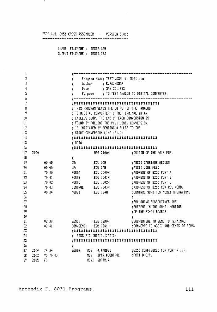
2500 A.D. 8051 CROSS ASSEMBLER - VERSION 3.0!c

' l 2

4 5 6 7 8 9

!Q 11 1" . ,. 13 !4 15 16 17 2100 18 !9

21

24 25 'H ~u

27

29 30 31

34 "'" ~•J -,L ·JU

00 OD 0(1 OA 70 00 70 01 70 02 70 03 00 B4

02 DO 02 41

J7 2100 74 B4 38 2102 90 70 03 39 2105 FO

INPUT FILENAME : TEST5.ASM OUTPUT FILENAME: TESTS.OBJ

·---------------------------------------------------------------------' Progra11 Na111e; TE5T4.ASM in 8031 asm Author Date Purpose

; R.RAJKUMAR ; MAY 25,1985 ; TO TEST ANALOG TO DIGITAL COl!\JERTER.

·---------------------------------------------------------------------' ;ttttttttttttttttttttttttttttt!tttttttittttttlttttt ; THIS PROGRAM SENDS THE OUTPUT OF THE ANALOG ; TO DIGITAL CONVERTER TO THE TERMINAL IN AN ; ENDLESS LOOP. THE END OF EACH CONVERSION IS ; FOUND BY POLLING THE Pl.! LINE. CONVERSION ; IS INITIATED BY SENDING A PULSE TO THE ; START CONVERSION LINE (Pl.Ol ;ttttttttttttttttttttttttttttttttttttttttttttttttt ; DATA ;ttttttttttttttttttttttttttttttttttttttttltttttttt

ORS 2100H ;ORIGIN OF THE ~AIN PGN.

CR: ,EQU OOH ;ASCII CARRIAGE RETURN LF: .EGU OAH ;ASCII LINE FEED PORTA .EQU 7000H ;ADDRESS OF 8255 PORT A PORTB .mu ?OO!H ;ADDRESS OF 8255 PORT B PORTC .EQU 7002H ;ADDRESS OF 8255 PORT C CONTROL . EQU 7003H ;ADDRESS OF 8255 CONTROL WORD .

;CONTROL ~ORD FOR MODE! OPERAiIOrt MOOE! .mu OB4H

:FOLLOWING SUBROUTINES ARE ;PRESENT IN THE SM-31 ;OF THE FX-31 BOARDS.

SDJD: .EOU 02DOH ;SUBROUTINE TO SEND TO TERMINAL. COMVSEND: . mu 0241H ; CONVERTS TO ASCII AND SENDS TO TERN. ;ttttttttltttttlttttttttttttttJtlt!ttt!tttttttttlt ; 8255 PIO INITIALIZATION ;ttttltttttttittlttttttttttttttttttttttttttttttttt

BE6IN: MOY A,#MODE! MOV DPTR,ICONTROL MG'IX @DPTR,A

: 8255 CONFIGURED FOR PORT A I/P, :PCRT B 0/P,


40 41 4Z

44 2106 45 210S

r"J Of! ...... ,· .• ·

D2 90 4b 210A 00 47 2108 C2 90

49 210D A2 91 50 210F 40 FC 51 52

55

2il4 2115

9r1 70 00 EO 12 (12 41

56 2118 74 OD 57 58 59

211A 211.!) 2l!F

12 02 DO 74 OA 12 02 DO

61 2122 21 06 62 63 2124

;if.tI!tf.tttttt!tttttt!ttttttlttt!ttt!tt!ttttttttit , '1AIN PROSRAN ;tttttt!tttttttttt!tttttttt!ttttttttttt!tttttttt!t START: CLR Pl.:)

SETS Pl I\ '••\.•

NOP CLR P1 /l

POLL: MOU C,Pl.1

.END

JC POLL

MOY DPTR,IPORTA MOVX A,~DPTR LCALL COtlVSEND

MOV A,llCR LCALL SEND MO\/ A,#LF LCALL SEND

Jl1P START

;SEND A PULSE TO ?1.0 :TO START CONVERSION.

;PDLL ECC T!LL LO.

;SEND THE CONVERTER Q/P ; FROM FORT A, ~FTER CONVERSION ;TO ASCII, TO THE TERM!NAL.

;SEND CR&LF.

;LOOP BACK TO START.

ttttlttlltttt SYN BO L IC REFERENCE TABLE ltttttttttltt

BESIN 2100 CONTROL = 7003 CONVSEND = 0241 CR = OOOD LF = OOOA MODEi = 0084 POLL 2100 PORTA = 7000 FORiB = 7001 PORTC = 7002 SEND = 02D0 START 2106

INES ASSEMBLED : 63 HSSE!'IBL Y ERRORS : 0


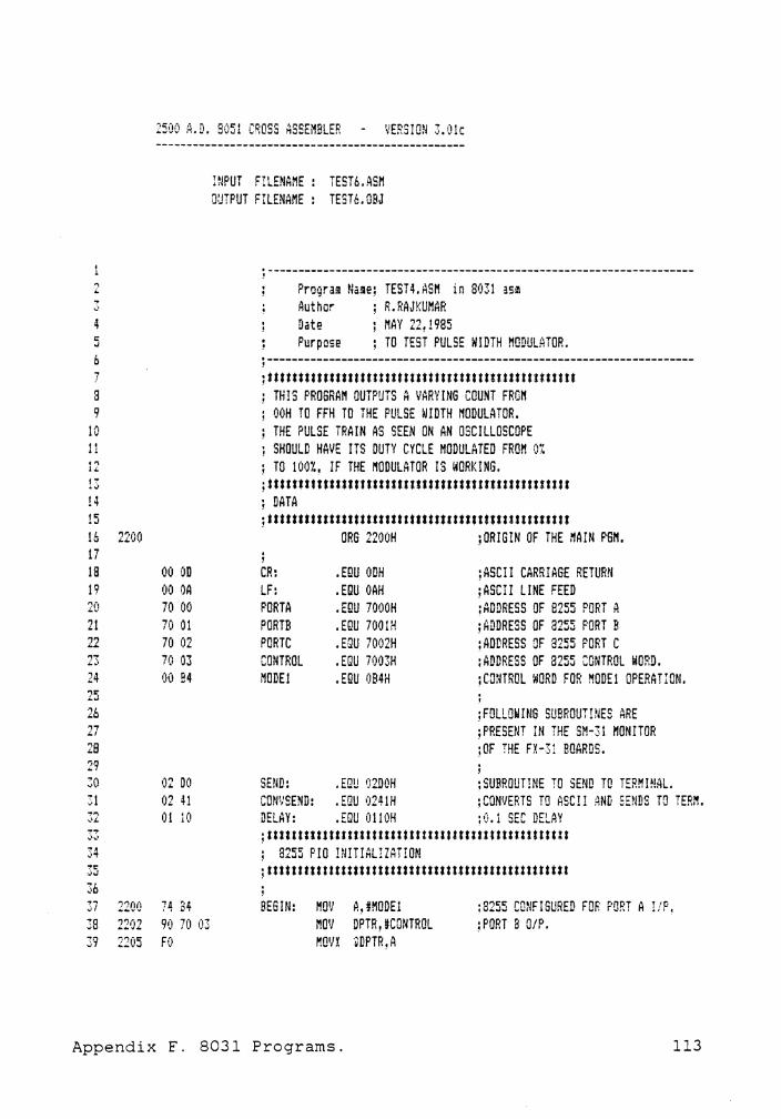
2500 A.D. 8051 CROSS ASSEMBLER - VERSION 3.0lc

4 5 6

8 9

14 15 16 221j(I 17 1B 00 OD 19 00 OA 20 70 00 21 70 01 22 70 02 23 70 03 24 00 B4

'17 .. , 2B 29 30 31

34

36 37 2200 38 22,)2 39 2205

02 DO 02 41 01 1(!

9(1 70 03 FO

INPUT FI LENA ME : TEST 6. ASM OUTPUT FILENAME: TEST6.0BJ

·---------------------------------------------------------------------!

Program Narae; TEST4.A5M in 8031 asi!I Author ; R. RAJ KUMAR Date Purpose

; MAY 22,1985 : TO TEST PULSE WIDTH MODULATOR.

·---------------------------------------------------------------------' ;ttttttttStttttttttttttttrttttJtttttttltttttttttttt THIS PROGRAM OUTPUTS A VARYING COUNT FR!JM

; OOH TO FFH TO THE PULSE ~J!DTH MODULATOR. ; THE PULSE TRAIN AS SEEN ON AN OSCILLOSCOPE ; SHOULD HAVE ITS DUTY CYCLE MODULATED FROM O'.! ; TO 10rJ%, IF THE NODULATOR IS WORKING. ;ttSStttttttttttttttttltttttttlttttlttSttlttt!tttt ; DATA ;lttStttttlttllttttttlttttltttlttttt!ttt!ltllttttt

CR: LF: PORTA PORTB PCP.TC CONTROL MODE!

ORS 2200H ;ORIS!N OF THE MAIN P6M.

.mu ODH

.mu OAH

.E9U 7000H

.mu 1001H

. mu 7002H • 7003H .mu OB4H

;ASCII CARRIAGE RETURN ;ASCII LINE FEED ;ADDRESS OF 8255 PORT A ;ADDRESS OF 8255 PORT B ;ADDRESS OF 8255 PORT C :ADDRESS OF 8255 CONTROL WORD . ; CONTROL WORD FOR MOOE! OPERATION.

;FOLLOWINS SUBROUTINES ARE ;PRESENT IN THE SM-31 MONITOR ;OF THE FY.-31 BOARDS.

SEND: . EQU 02DOH : SUBROUT! NE TO SEND TO TERM !Nill. CON\/SEND: .mu 0241H :CON\JERTS TO ASCII AND mrns TO TERl'!. DELAY: .mu 0110H :0.1 SEC DELAY ;tttttttttttttttttttttttttttlttlttttlttttttttttttt ; 8255 PIO INITIAL!ZAT!ON ;tttttttttttttttttttttttttttttttlttttttttttttttttt

MDV A,#MODE1 MDV DPTR,#CONTROL M01H ~DPTR, A

: 3255 CONF I SURED FOF: PORT A !/ P, ;PORT B 0/P.


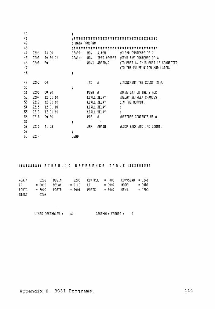
40 41 42 43 44 1206 74 0(1

45 46 47 48

49 5() 51 .,.,. .J,j

54 55 C:L wU

57 59 59 60

2208

2200 220F 2212 2215 2218 221B

2210

90 70 O! FO

CO EO 12 01 10 !2 01 10 12 01 10 12 01 ! 0 00 E(l

41 08

;itttttttSttttit!lttttttt!tt!titttittttt!ttttttttt , MAIN PROGRAM ;!tttttttlttttttttlttttt!i!tttttttltttttttttttt!St START: MDV A,IOH ;CLEAR CONTENTS QF A

.END

MO!/ DPTR,#POP.TB MOVX ~DPTR,A

PUSH A LCALL DELAY LCALL DELAY LCALL DELAY LCALL DELAY POP A

JMP AGAIN

;SEND THE CONTENTS OF A ;TO PORT A. THIS PORT IS CONNECTED ;TO THE PULSE WIDTH MODULATOR.

;INCREMENT THE CCUNT !NA.

;SAVE (AJ ON THE STACK ;DELAY BETWEEN CHANGES ; IN THE OUTPUT .

; RESTORE COIHEtHS OF A

;LOOP BACK AND !NC COUNT.

tltttttattttt SYMBOLIC REFERENCE TABLE ttttttttttltt

AGAIN 2208 BEGIN 2200 CONTROL = 7003 CONVSEND = !)241 ci;; " = 000D DELAY = 0110 LF = OOOA f10DE! = OOB4

PORTA = 70(!0 PORTB = 7001 PORTC = 7002 SEMD = 0200 START 2206

LINES ASSEMBLED : 60 ASSEMBLY ERRORS : i)


BIBLIOGRAPHY

1. Allen Systems FX-31 Users Manual Allen Systems, Columbus, Ohio. 1984.

2. Berk,A.A. The Art of Micro Design. Published by Newness, U.K. 1984.

3. Coiffet,P. and Chirouze,M. 1982 - An Introduction to Robot Technology. Published by Hermes Publishing. 1982.

4. General Electric P-50 Process Robot Maintenance and Installation Manual 1984.

5. General Electric P-50 Process Robot Operator's Manual 1983.

6. Hopkins,M.A. 1984 - An Improved Controller for the Rhino Robot Arm. Masters Thesis, Virginia Tech. 1984.

7. IBM PC Technical Reference. Published by IBM Corp. 1983.

8. Intel 1983.Microcontroller Handbook. Published by Intel Corporation. 1983.

9. Johnson,C. 1984 - Microprocessor Based Control Systems. Published by Prentice Hall,Inc. 1984.

10. Koren,Yoram. 1985 - Robotics for Engineers. Published by McGraw Hill Book Company.

11. Kuo,C.B. 1980 - Digital Control Systems. Published by Holt, Rinehart and Wingly, Inc. 1980.

12. Lee,C.S.G. 1983 - "On the Control Of Robot Manipula-tor". Proc. of 13th International Symposium on Indus-trial Robots 1983.

13. Lee,C.S.G. 1982 - "Robot Arm Kinematics, Dynamics and Control". IEEE COMPUTER Magazine Dec 1982 .

14. Lee,C.S.G et al. 1983 - Tutorial on Robotics. Published by IEEE Computer Society Press. 1983.

15. Lumelsky, Vladmir J. 1983 - "Control of Robot Motion". Pree.13th International Symposium on Industrial Robots 1983.

Bibliography 115

16. Paul, R. 1981- Robot Manipulators; Mathematics, Pro-gramming and Control. Published by MIT Press 1981.

17. Pugh,A. 1983 - Robotic Technology. Published by Peter Peregrinus Ltd; London, U.K.

18. Snyder, W. 1980 - "Micro-Computer Based Path Control".

19.

Robotics Age, Vol 2, Number 1, Spring 1980.

Snyder,W. Encoders".

and Schott, J. 1980 - "Using Optical Shaft Robotics Age, Vol 2, Number 3, Fall 1980.

20. Technical Data Base Corp. Robotics Industry Directory 1982.

21. Vukobratovic, M and Stokic ,D. Scientific Fundamentals of Robotics Vol2. Published by Springer-Verlag 1982.

22. Whitney,D.E 1969 - "Resolved Motion Rate Control of Manipulators and Human Prosthesis". IEEE Trans. Man-Machine Systems June 1969.

23. Zewari,S.W Planning".

1985(a)- "Robot's Kinetics and Trajectory Proc. Robots 9, June 2-6 1985, Detroit.

24. Zewari,S.W 1985(b)- "The Ins and Outs of Robot Kinematics". Proc. 1985 ASME International, Computers in Engineering, Conference and Exhibition.

25. Zewari, S. W 1984 - "Side Effects of Trajectory Plan-ning". Proc. 1984 ASME International, Computers in Engineering Conference and Exhibition.

26. Zewari, S. W 1984 - Class Notes of "Introduction to Robotics" at Virginia Polytechnic Institute and State University.

27. Zewari, S. W 1984 - "Dual Mode Servo Control System". Proc. American Control Conference, San Diego, June 6-8 1984.

28. Zewari,S.W 1984 - "Robot Positioning as a Transforma-tion Problem". Proc. 1984 ASME International, Computers in Engineering, Conference and Exhibition. Vol2.

Bi]?liography 116

The vita has been removed from the scanned document

for the p-50 industrial robot by

Documents