forces - rice university · pdf fileit is a non‐procedural ... you need to write as many...

Bedford, Fowler: Statics. Chapter 3: Forces, Examples via TK Solver

Copyright J.E. Akin. All rights reserved. of 23

Forces

Introduction

In this chapter, solutions are obtained by direct application of Newton’s Laws. In a later chapter, an alternate solution approach based on “Energy Methods” will be introduced. Modern numerical methods for solving mechanics problems often rely primarily on energy methods, and use Newton’s Laws only as necessary validation checks. However, for small or simple systems, like those illustrated in this chapter, direct application of Newton’s Laws is usually the quickest way to reach a solution.

Example 3.1

The system of plane, automobile, and cable represent a resultant system of three forces that are concurrent (pass through a common point). They are shown in Figure 1. The system is at rest, so the acceleration is zero, and so it is referred to as a statics problem. The plane actually applies normal (perpendicular) forces to the front and rear wheels. However, they combine to form a single normal force, N. (Later you will learn how to find both of the normal wheel forces.) The plane makes an angle of 20 degrees up from horizontal. Thus, the normal force is at an angle of 20 degrees to the left of vertical. This is a two‐dimensional model with a single free body diagram (FBD), which is given in Figure 2. Therefore, you have only three laws (rules) available: gravity and equilibrium in the horizontal (x‐) and vertical (y‐) directions.

Figure 1 Inclined automobile sketch Figure 2 FBD of concurrent forces

Later you will have many FBD’s to employ with several rules that apply to each. Therefore, it is desirable to have a computer tool for crunching numbers, while you concentrate on the mechanics principles that give you the rules that are necessary to solve a statics or dynamics problem.

TK Solver is just such a tool. It is a non‐procedural “case solver”, and not a programming language. Modern engineering programming languages like, Fortran 2003, and C++ (as well as the Matlab environment), require all their statements to be in a strict procedural (sequential) order. Any current statement can only refer to variables defined by previous statements. Furthermore, a programming statement can have only one variable to the left of the equals (=) assignment sign. None of those programming restrictions applies to TK rules. TK Solver rules can (and should) be written as you



think of them as governing principles. The equals (=) sign can be anywhere in the rule. So, place it where you are used to seeing it in a governing principle. Also, remember that any good engineering coding style should contain about 50% comments as self‐documentation. In TK, a semi‐colon (;) precedes a comment at the end of a rule.

TK Solver is called a ‘case‐solver’ because it counts the number of unknowns and searches the rules to find enough equations to compute them. It also does that search in an efficient way. It first looks for a single valid equation to solve. Finding none it would search for two simultaneous equations to solve. If that fails it searches for three, and so on. When it solves a case, its successful solution reduces the number of unknowns, so it repeats its case search. Sometimes the system of simultaneous equations is solved by iteration and you start that process by assigning a Guess value to one or more selected variables.

You should always try to count the number of unknowns. You need to write as many equilibrium equations as there are unknowns. Here, there are two unknowns: the cable force and the resultant normal force from the plane. For the class of problems in this chapter, there are two equilibrium equations per FBD. Thus, you need (and have) only one FBD. The TK rules for this example are shown in Figure 3. As each rule is completed (by an ‘Enter’ key), the name of each new variable automatically begins the population of the variable sheet. The initial variable sheet appears in Figure 4. Applying the usual Windows ‘cut‐and‐paste’ procedures, you can move rows around later for a pretty report. The variable sheet shows that any variable could be selected as a known quantity to have an input numerical value assigned to it. If a variable is not input, then TK Solver will try to compute its output value.

Figure 3 Rules for the inclined automobile

There is one important aspect of assigning units to a variable. TK Solver allows you to compute using one set of consistent units, and display the (input or output) in any other units. You can use any units (within reason as described below), BUT the first time you put a unit (symbol) in the Unit column of the Variable Sheet, that unit is the one used for calculation unit. Here, that is important because you are using trigonometric functions that expect radians as arguments. Therefore, you must enter ‘radians’ or ‘rad’ as the computation (first) unit for the variable angle.



Figure 4 The initial variables sheet

A completed Variables Sheet is in Figure 5. After first entering the calculation units, you can re‐enter display units for any variable. Select enough input items to make the problem solvable, and assign them numerical input values.

Attempt to find the outputs by executing a TK ‘direct solve’, by clicking on the light bulb icon, . Then, all the output variables found will appear. It is important to note here that the output forces had positive signs. That means that the corresponding assumption of tension or compression was correct. When in doubt, it is a good practice to assume any unknown force is in tension. Then, a negative output value would show that it is actually in compression. Remember, that the usable number of significant figures in the output cannot exceed the number available in the inputs. The bottom three comment lines in Figure 5 illustrate the power of TK to let you play the necessary engineering game of “what‐if”. What‐if the cable has a safe load limit of 5,000 N.? What is the maximum angle for building the ramp?

Figure 5 Variables with input choices and display unit choices

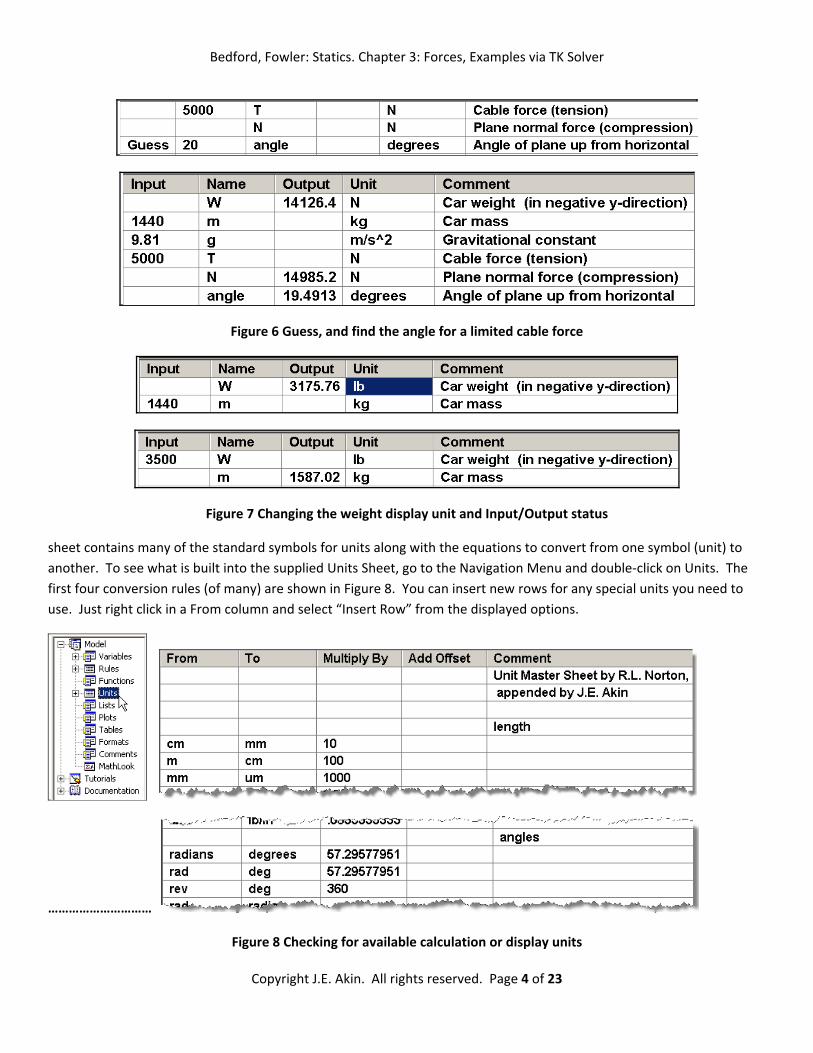
The result of such an engineering study is given in Figure 6. Likewise, the TK model can be used to check your common sense expectations for the mechanics principles. What would you expect the cable and plane forces to become if you set the angle to zero? (Try it.) Likewise, your boss may ask, what is the weight in pounds? Figure 7 shows that you just have to change the output unit to lb to see that the answer is about 3,176 lb. Or, you can specify the weight in pounds and solve for its mass. You can download this completed example workbook from file Bedford_Chap_3_1.tkw. Better still, begin with a blank workbook containing just the most common units symbols sub‐sheet, and add your own rules like shown above. That file name is Units_only.tkw. Just save it with a new name after you have begun your application.

Now, some more words to the wise about units in TK Solver. Units are just character strings or symbols. Therefore, if you make a typo in entering units you have defined a new engineering unit. If TK cannot find a conversion in the Units Sheet you will see a question mark (?) before a numerical value showing that the value is probably wrong. The units



Figure 6 Guess, and find the angle for a limited cable force

Figure 7 Changing the weight display unit and Input/Output status

sheet contains many of the standard symbols for units along with the equations to convert from one symbol (unit) to another. To see what is built into the supplied Units Sheet, go to the Navigation Menu and double‐click on Units. The first four conversion rules (of many) are shown in Figure 8. You can insert new rows for any special units you need to use. Just right click in a From column and select “Insert Row” from the displayed options.

…………………………

Figure 8 Checking for available calculation or display units



Sometime you will forget to enter the calculation unit first into the Variable Sheet. Then, you will need to change it. To do so, right‐click on the variable name and select its Sub sheet. There, you can assign any symbol in the Units Sheet to be the calculation and/or display unit. They are shown in Figure 9.

Figure 9 Define or change a variable calculation or display unit TK Solver includes a “Report Wizard” (File Create Report) to provide neat written reports. See the help file for the options. A simple default report for this example is given in the Appendix. Example 3.2

Again, the system in this example is three concurrent forces in a vertical plane. The same three principles apply, just the two equilibrium rules change. The engine block support ropes and their FBD are given in Figure 10. Here, there are two unknowns: the forces in the inclined ropes. (By inspection, you should see that the vertical force carries the full weight. If you do not see that, draw a second FBD of just the weight and the vertical cable.) Like the prior example, you need only one FBD to define the equilibrium rules. The corresponding Rule Sheet is in Figure 11 and the assigned units are in

Figure 12. Executing by clicking solve, , gives the results in Figure 13.

Figure 10 Cable supported engine block

Again, it is always wise to check a model with common sense tests. For example, if the left cable was vertical you should expect it to support the entire weight. Then the right cable should carry no portion of the weight (unless the wind blows and we modify the FDB). Check that case by setting the left angle to 90 degrees, and solve again (as in Figure 14). The



completed worksheet for this example has file name Bedford_Chap3_2.tkw. While you can use it to duplicate these figures, you will learn more by building your own worksheet by starting with the default work sheet (Units_only.tkw).

Figure 11 Gravity and equilibrium rules

Figure 12 Initially populated Variable Sheet with an initial guess

Figure 13 A solution for a pair of active ropes

Figure 14 The solution for the left rope vertical



Hint for Debugging Rules

Everyone makes a mistake sometime, so consider a debugging trick. If an expression should equal zero, equate it equal to an error variable name instead. You can always input the error variable as zero. When your rules are debugged, you can equate the expression exactly to zero, in the Rules Sheet, and delete the rows with the error variables, in the Variable Sheet. To illustrate such an approach let the last rule have a sign error in the second term, as in Figure 15 (top). The horizontal equilibrium equation is the simplest. Try setting its error to zero and guess a value of 100 N for T_AC. While a solution is obtained, there is a large negative (downward) error in the y‐direction, as seen at the bottom of Figure 15. That suggests that one (or both) of the vertical cable forces may be in error. Correcting the AB tension vertical sign and setting both error variables to zero yields the results in the text, and in Figure 13 above.

Figure 15 Correcting the sign error and setting both error values to zero yields a solution

List Solves and Graphs

You may be interested in looking at the results for a range of angles for the rope AB. You may also wish to graph those results. To illustrate that process assume you wish to vary the AB angle from 45 to 90 degrees while keeping the weight and AC angle constant (by changing the length of AC). Clearly, forces T_AB and T_AC will vary as angle BA varies. In other words, there will be one input list (for angle_BA) and two output lists (for T_AB and T_AC). To indicate that task,



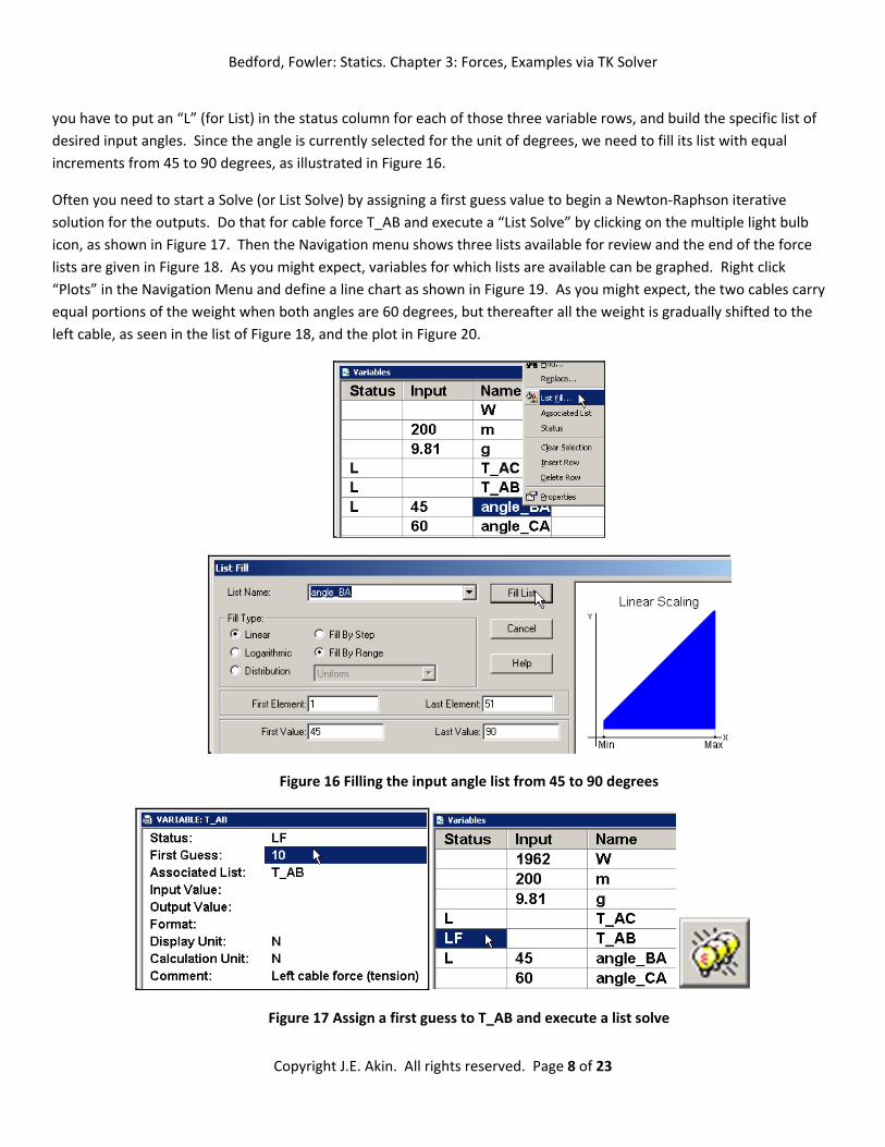
you have to put an “L” (for List) in the status column for each of those three variable rows, and build the specific list of desired input angles. Since the angle is currently selected for the unit of degrees, we need to fill its list with equal increments from 45 to 90 degrees, as illustrated in Figure 16.

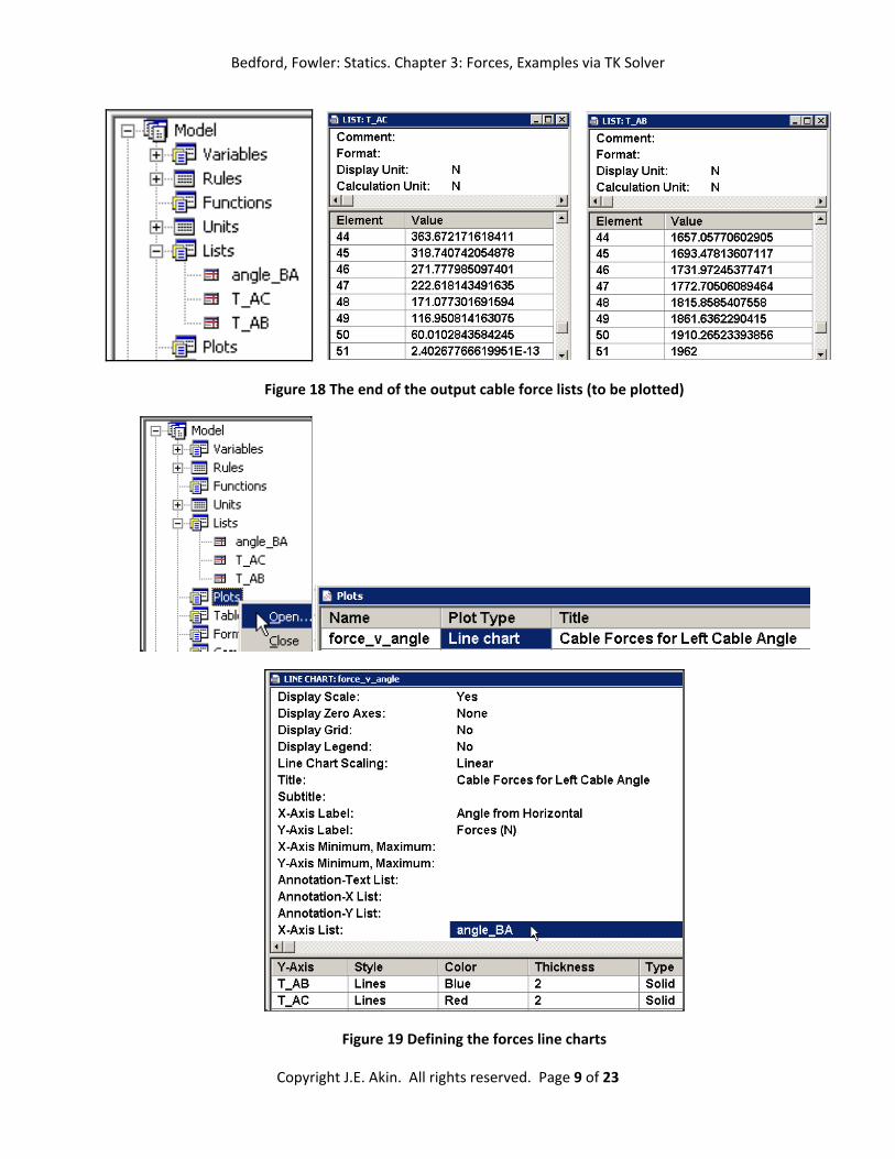
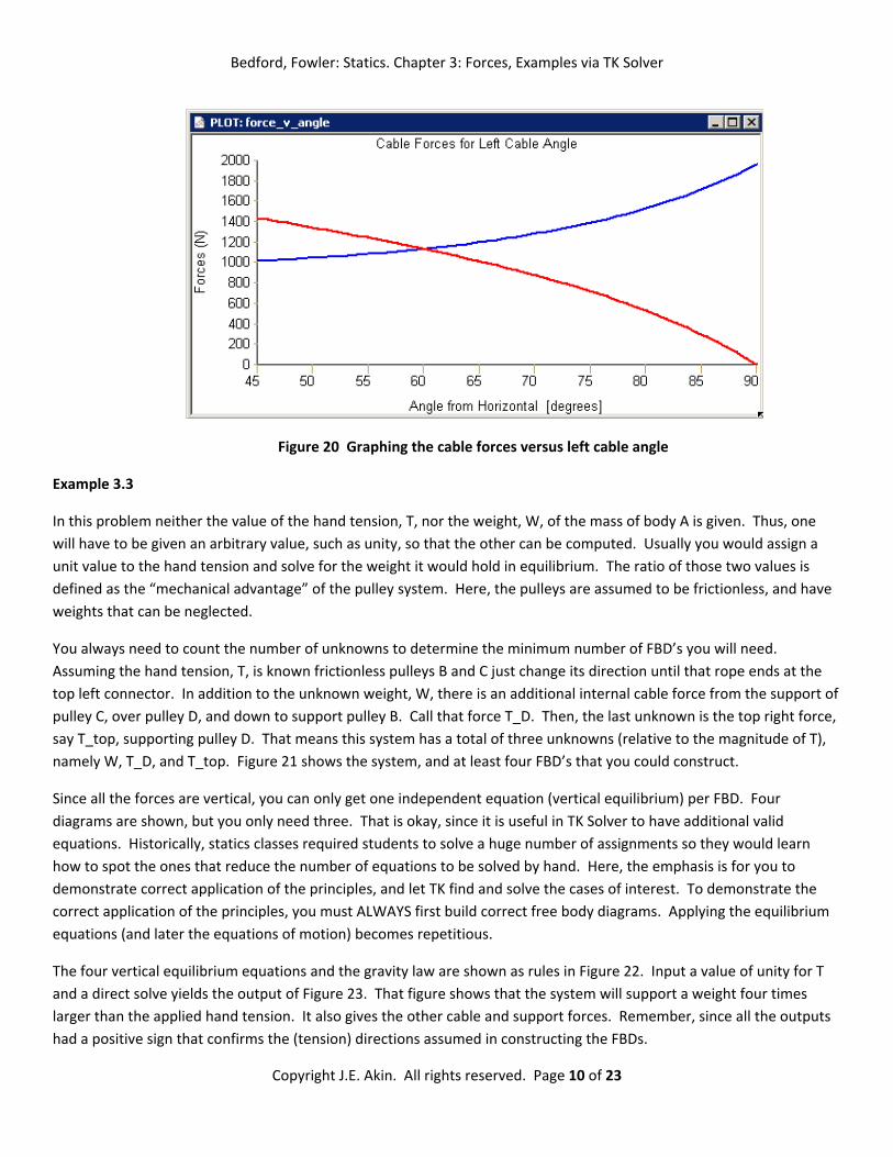
Often you need to start a Solve (or List Solve) by assigning a first guess value to begin a Newton‐Raphson iterative solution for the outputs. Do that for cable force T_AB and execute a “List Solve” by clicking on the multiple light bulb icon, as shown in Figure 17. Then the Navigation menu shows three lists available for review and the end of the force lists are given in Figure 18. As you might expect, variables for which lists are available can be graphed. Right click “Plots” in the Navigation Menu and define a line chart as shown in Figure 19. As you might expect, the two cables carry equal portions of the weight when both angles are 60 degrees, but thereafter all the weight is gradually shifted to the left cable, as seen in the list of Figure 18, and the plot in Figure 20.

Figure 16 Filling the input angle list from 45 to 90 degrees

Figure 17 Assign a first guess to T_AB and execute a list solve



Figure 18 The end of the output cable force lists (to be plotted)

Figure 19 Defining the forces line charts



Figure 20 Graphing the cable forces versus left cable angle

Example 3.3

In this problem neither the value of the hand tension, T, nor the weight, W, of the mass of body A is given. Thus, one will have to be given an arbitrary value, such as unity, so that the other can be computed. Usually you would assign a unit value to the hand tension and solve for the weight it would hold in equilibrium. The ratio of those two values is defined as the “mechanical advantage” of the pulley system. Here, the pulleys are assumed to be frictionless, and have weights that can be neglected.

You always need to count the number of unknowns to determine the minimum number of FBD’s you will need. Assuming the hand tension, T, is known frictionless pulleys B and C just change its direction until that rope ends at the top left connector. In addition to the unknown weight, W, there is an additional internal cable force from the support of pulley C, over pulley D, and down to support pulley B. Call that force T_D. Then, the last unknown is the top right force, say T_top, supporting pulley D. That means this system has a total of three unknowns (relative to the magnitude of T), namely W, T_D, and T_top. Figure 21 shows the system, and at least four FBD’s that you could construct.

Since all the forces are vertical, you can only get one independent equation (vertical equilibrium) per FBD. Four diagrams are shown, but you only need three. That is okay, since it is useful in TK Solver to have additional valid equations. Historically, statics classes required students to solve a huge number of assignments so they would learn how to spot the ones that reduce the number of equations to be solved by hand. Here, the emphasis is for you to demonstrate correct application of the principles, and let TK find and solve the cases of interest. To demonstrate the correct application of the principles, you must ALWAYS first build correct free body diagrams. Applying the equilibrium equations (and later the equations of motion) becomes repetitious.

The four vertical equilibrium equations and the gravity law are shown as rules in Figure 22. Input a value of unity for T and a direct solve yields the output of Figure 23. That figure shows that the system will support a weight four times larger than the applied hand tension. It also gives the other cable and support forces. Remember, since all the outputs had a positive sign that confirms the (tension) directions assumed in constructing the FBDs.



Figure 21 A vertical pulley system and some FBD’s

Figure 22 Rules for the three‐pulley system

Figure 23 The system has a mechanical advantage of four (W/T)

If you had only cared about the value of the supported weight, then an experienced analyst would have seen that you only needed two FBD’s (2 and 3) and two rules. That experience will come in time, but now just concentrate on the principles and let TK solve the systems. If you fail to provide enough rules, then TK will not provide outputs. That will be



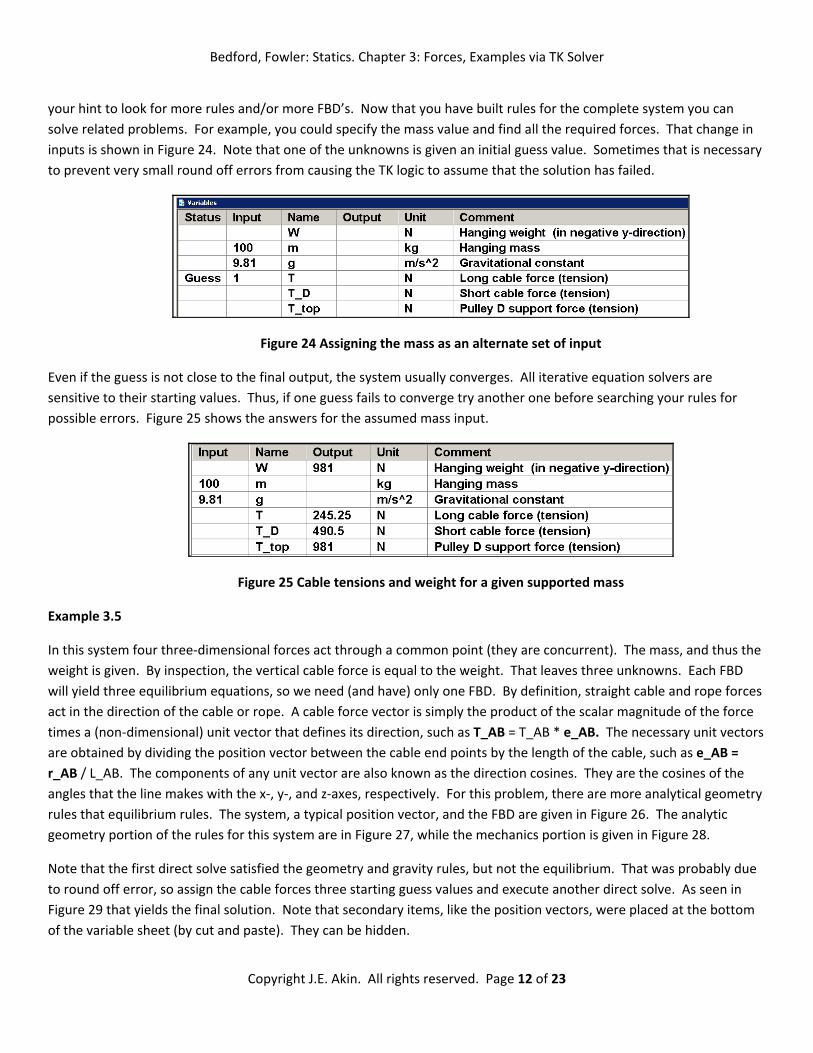
your hint to look for more rules and/or more FBD’s. Now that you have built rules for the complete system you can solve related problems. For example, you could specify the mass value and find all the required forces. That change in inputs is shown in Figure 24. Note that one of the unknowns is given an initial guess value. Sometimes that is necessary to prevent very small round off errors from causing the TK logic to assume that the solution has failed.

Figure 24 Assigning the mass as an alternate set of input

Even if the guess is not close to the final output, the system usually converges. All iterative equation solvers are sensitive to their starting values. Thus, if one guess fails to converge try another one before searching your rules for possible errors. Figure 25 shows the answers for the assumed mass input.

Figure 25 Cable tensions and weight for a given supported mass

Example 3.5

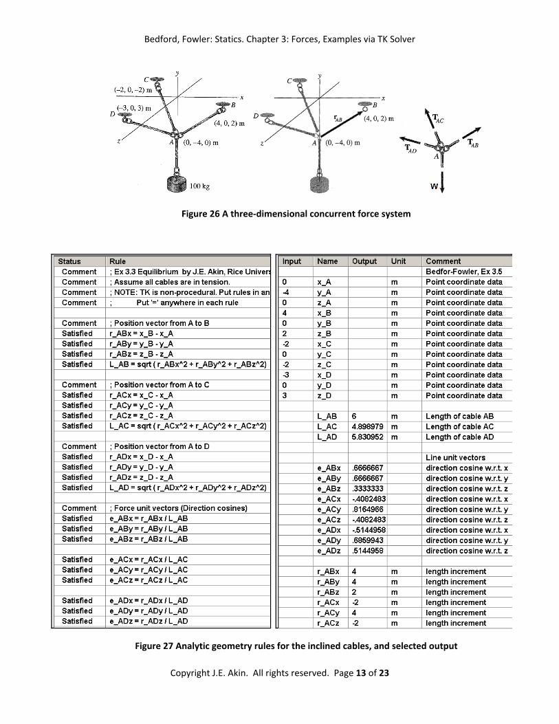
In this system four three‐dimensional forces act through a common point (they are concurrent). The mass, and thus the weight is given. By inspection, the vertical cable force is equal to the weight. That leaves three unknowns. Each FBD will yield three equilibrium equations, so we need (and have) only one FBD. By definition, straight cable and rope forces act in the direction of the cable or rope. A cable force vector is simply the product of the scalar magnitude of the force times a (non‐dimensional) unit vector that defines its direction, such as T_AB = T_AB * e_AB. The necessary unit vectors are obtained by dividing the position vector between the cable end points by the length of the cable, such as e_AB = r_AB / L_AB. The components of any unit vector are also known as the direction cosines. They are the cosines of the angles that the line makes with the x‐, y‐, and z‐axes, respectively. For this problem, there are more analytical geometry rules that equilibrium rules. The system, a typical position vector, and the FBD are given in Figure 26. The analytic geometry portion of the rules for this system are in Figure 27, while the mechanics portion is given in Figure 28.

Note that the first direct solve satisfied the geometry and gravity rules, but not the equilibrium. That was probably due to round off error, so assign the cable forces three starting guess values and execute another direct solve. As seen in Figure 29 that yields the final solution. Note that secondary items, like the position vectors, were placed at the bottom of the variable sheet (by cut and paste). They can be hidden.



Figure 26 A three‐dimensional concurrent force system

Figure 27 Analytic geometry rules for the inclined cables, and selected output



Figure 28 Mechanics rules for the hanging mass

Figure 29 Final iterative three‐dimensional concurrent system cable results

This example is available as file name Bedford_Chap_3_5.tkw. Having verified a valid model it can be used for other purposes. Assume that you measured the force in cable AC to be 700 N, and you need to know the weight (and/or other two cable forces). The resulting four outputs are given in Figure 30, for that case.

Figure 30 Using a measured cable force to find the mass



Example 3.6

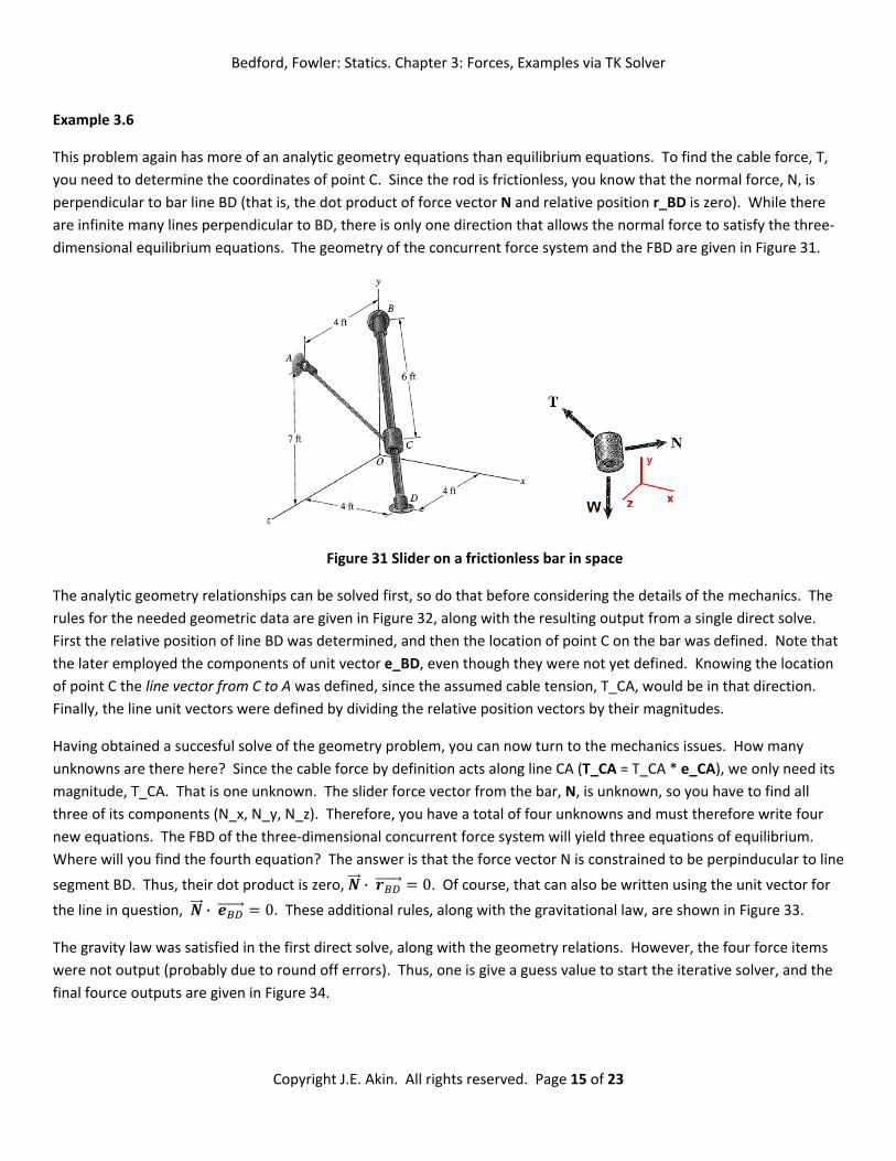
This problem again has more of an analytic geometry equations than equilibrium equations. To find the cable force, T, you need to determine the coordinates of point C. Since the rod is frictionless, you know that the normal force, N, is perpendicular to bar line BD (that is, the dot product of force vector N and relative position r_BD is zero). While there are infinite many lines perpendicular to BD, there is only one direction that allows the normal force to satisfy the three‐dimensional equilibrium equations. The geometry of the concurrent force system and the FBD are given in Figure 31.

Figure 31 Slider on a frictionless bar in space

The analytic geometry relationships can be solved first, so do that before considering the details of the mechanics. The rules for the needed geometric data are given in Figure 32, along with the resulting output from a single direct solve. First the relative position of line BD was determined, and then the location of point C on the bar was defined. Note that the later employed the components of unit vector e_BD, even though they were not yet defined. Knowing the location of point C the line vector from C to A was defined, since the assumed cable tension, T_CA, would be in that direction. Finally, the line unit vectors were defined by dividing the relative position vectors by their magnitudes.

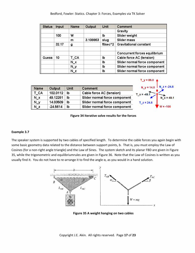
Having obtained a succesful solve of the geometry problem, you can now turn to the mechanics issues. How many unknowns are there here? Since the cable force by definition acts along line CA (T_CA = T_CA * e_CA), we only need its magnitude, T_CA. That is one unknown. The slider force vector from the bar, N, is unknown, so you have to find all three of its components (N_x, N_y, N_z). Therefore, you have a total of four unknowns and must therefore write four new equations. The FBD of the three‐dimensional concurrent force system will yield three equations of equilibrium. Where will you find the fourth equation? The answer is that the force vector N is constrained to be perpinducular to line

segment BD. Thus, their dot product is zero, · 0. Of course, that can also be written using the unit vector for the line in question, · 0. These additional rules, along with the gravitational law, are shown in Figure 33.

The gravity law was satisfied in the first direct solve, along with the geometry relations. However, the four force items were not output (probably due to round off errors). Thus, one is give a guess value to start the iterative solver, and the final fource outputs are given in Figure 34.



Figure 32 Slider‐bar analytic geometry rules and outputs

Figure 33 Equilibrium and force constraint relationships

Since the three‐dimensional FBD is difficult to visualize, you may want to draw the true shape projections of the FBD onto the XY, XZ, and YZ planes. To do that you need additional rules to get the components of tension T_CA (try it). This worksheet is stored with file name Bedford_Chap_3_6.tkw.



Figure 34 Iterative solve results for the forces

Example 3.7

The speaker system is supported by two cables of specified length. To determine the cable forces you again begin with some basic geometry data related to the distance between support points, b. That is, you must employ the Law of Cosines (for a non‐right angle triangle) and the Law of Sines. The system sketch and its planar FBD are given in Figure 35, while the trigonometric and equilibriumrules are given in Figure 36. Note that the Law of Cosines is written as you usually find it. You do not have to re‐arrange it to find the angle α, as you would in a hand solution.

Figure 35 A weight hanging on two cables



Figure 36 Equilibrium and trigonometry relations

You should observe that as the angles approach zero the cable forces would have to approach infinity. No material is that strong. Here it is given that cable forces may not exceed the value of the weight. As a reminder of that design limit, two extra variables (Ratio_AB, Ratio_AC) were defined to give the ratio of each cable force and the weight. To find the minimum angles (and lengths) that could be used, the two ratios were set equal to unity and the problem was solved, as seen in Figure 37. The two angles were 30 degrees, the length were about 1.16 m, and the two cable forces indeed equaled the weight.

Figure 37 Find the minimum design angles

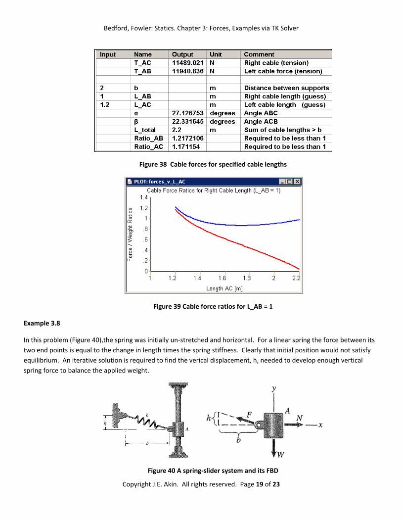
When the example cable lengths are specified to be 1 and 1.2 m, as in Figure 38, then the cable forces are above the given design limit. By varying the length of AC you can graph the the cable force to ratios as in Figure 39.



Figure 38 Cable forces for specified cable lengths

Figure 39 Cable force ratios for L_AB = 1

Example 3.8

In this problem (Figure 40),the spring was initially un‐stretched and horizontal. For a linear spring the force between its two end points is equal to the change in length times the spring stiffness. Clearly that initial position would not satisfy equilibrium. An iterative solution is required to find the verical displacement, h, needed to develop enough vertical spring force to balance the applied weight.

Figure 40 A spring‐slider system and its FBD



The simple geometry and equibrium rules are in Figure 41. To start an iterative solution for the vertical deflection of the weight just assign a guess value to h. Then you obtain the results in Figure 42.

Figure 41 Spring‐slider equiblirum

Figure 42 Starting a iterative solution and obtaining the deflection and forces



You probably recall from physics that you can describe the energy stored in the spring and the mechanical work done by lowering the weight. You could add rules for those items to the TK model, and plot them for a range of displacement values. Those actions are given in Figure 43. Note that the value of h (0.451 ft) obtained above as the equilibrium position is also the h value for the minimum position on the graph. The important preview here is that the state of equilibrium mimimizes the Total Potential Energy of a system. That principle will be used in later chapters as an alternative to the direct application of Newton’s Laws. The Principle of Minimum Total Potential Energy has the advantage that it can be applied to systems that are statically indeterminant. Such systems require consideration of the deformation of bodies in the system, like the spring in this example.

Figure 43 Equilibrium minimizes the total potential energy



Appendix: Creating quick reports or hardcopies

forces - rice university · pdf fileit is a non‐procedural ... you need to write as many...

Documents