Forecasting with an Economic Model and the Role of Adjustments

Andrew P. Blake

CCBS/HKMA May 2004

What is a forecast?• An assessment of the unknown

– Usually of variables only known in the future– Often probabilistic

• Forecast could be just a series of numbers

• Could be a forecast of the distribution of possible outcomes

• Forecasters therefore produce point, interval and density forecasts– Bank of England fan chart is a density forecast

What are adjustments?

• Adjustments are needed because we use judgement

• This may be imposed using information from outside the model– It may reflect model inadequacy– It may reflect data inadequacy– It may reflect expert opinion

Forecasting framework• How could we make forecasts?

– ‘Make them up’• Assess (a subset of) available data and judgement to produce

forecast

– Use a (statistical) model

• Forecast horizons– ‘Nowcasting’: forecasting current or past but unknown

data– Otherwise one minute to a hundred years

• Hundred year horizon unlikely to be very accurate

Modeling framework• What kinds of models are relevant?

– Statistical and econometric– Univariate and multivariate– Structural and reduced form

• Tools– Spreadsheets– Eviews, TSP, PcGive– Gauss, Matlab, Ox– WinSolve, Troll, Dynare

The process of forecasting

• Where do you start?– Previous forecast:

• Existing data, existing model

• New data, new model?

– ‘From scratch’

• What has changed since the last time?– Impact of ‘news’

• Sources of shocks

The process of forecasting (cont.)

• How do we incorporate news?– Updates to historical data– Previously unavailable data– Revisions to the model

• Previous failures may need correcting

– ‘Adjustments’ to the forecast• From non-model data

• Judgement

Simple forecasting

• Univariate models– ARIMA modeling– Exponential smoothing (more weight on recent

observations)

• Clements and Hendry suggest that

fits economic data well. For forecasting use:ttt yy 1

02 ty

Simple forecasting (cont.)

• Simple multivariate models– VAR widely used– Easy to re-estimate/update– Models have straightforward interpretation

• Minimum intervention needed– Properties depend on few choice variables– Benchmark forecast

VAR forecast

Data Residuals Forecast

Interest rate

Inflation rate

What do the residuals tell us?

• Tell us about the goodness-of-fit of the model

• Very useful over the recent past which may not be used in model estimation– May be going ‘off-track’

• Use in determining adjustments for a forecast

More sophisticated forecasting

• Structural Economic Model (SEM)– Multiple equations (2 to 5000)– Estimated/calibrated/imposed coefficients– Rich dynamics– Expectations – Complex accounting structures

• Complicated to use– Institutional and technical considerations

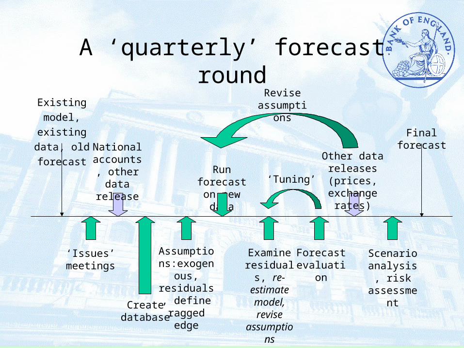
Existing model,

existing data, old

forecast Final forecastNational accounts, other data

release

Run forecast on new data

Examine residuals,

re-estimate model, revise

assumptions

Other data releases (prices, exchange rates)

A ‘quarterly’ forecast round

Assumptions:exogenous, residuals,

define ragged edge

‘Issues’ meetings

Create database

Forecast evaluation

Scenario analysis,

risk assessment

‘Tuning’

Revise assumptions

‘Week 0’

New data, same old problems• ‘Issues’ meetings

– Where have previous forecast failed?

– Where has the forecast model failed?

• New data– Start of forecast often determined by release dates, e.g.

National Accounts

– Create model database (transforms etc)

– Make ‘first quarter’ assumptions• Expert analysis

• Partial information

The ‘ragged edge’

Old data New/revised data Assumptions

Forecast date

Time

Dealing with the ragged edge

• Exogenise all past true data values– Incorporate historical add factors

• Exogenise ‘first quarter’ assumed data

• Exogenise future assumptions

• Solve the model from far enough back

News: data revisions• The past isn’t always what it used to be

– ‘Real time’ data sets show significant changes• Eggington, Pick & Vahey, 2002

• Castle & Ellis, 2002, Band of England QB

• Question of what you wish to forecast– Do you wish to forecast the first outturn or final

estimate?– Markets may react less strongly to revised data

than ‘new’ data

Data revisions

‘Week 1’

Old model, same old problems• Exogenous variable assumptions

– All things exogenous to the model– Rest of the world, policy variables, fiscal authorities

• ‘Residuals’– Adjustments or add-factors– Constant values, future profiles– Helps robustify to structural breaks (Clements and

Hendry)• ECMs helpful in this respect

Adjustments

• What does the model tell us about how our forecast may be failing?

• Need to look at the implicit residuals

• We need to ensure that any adjustments are consistent with the model – or have a good reason why not

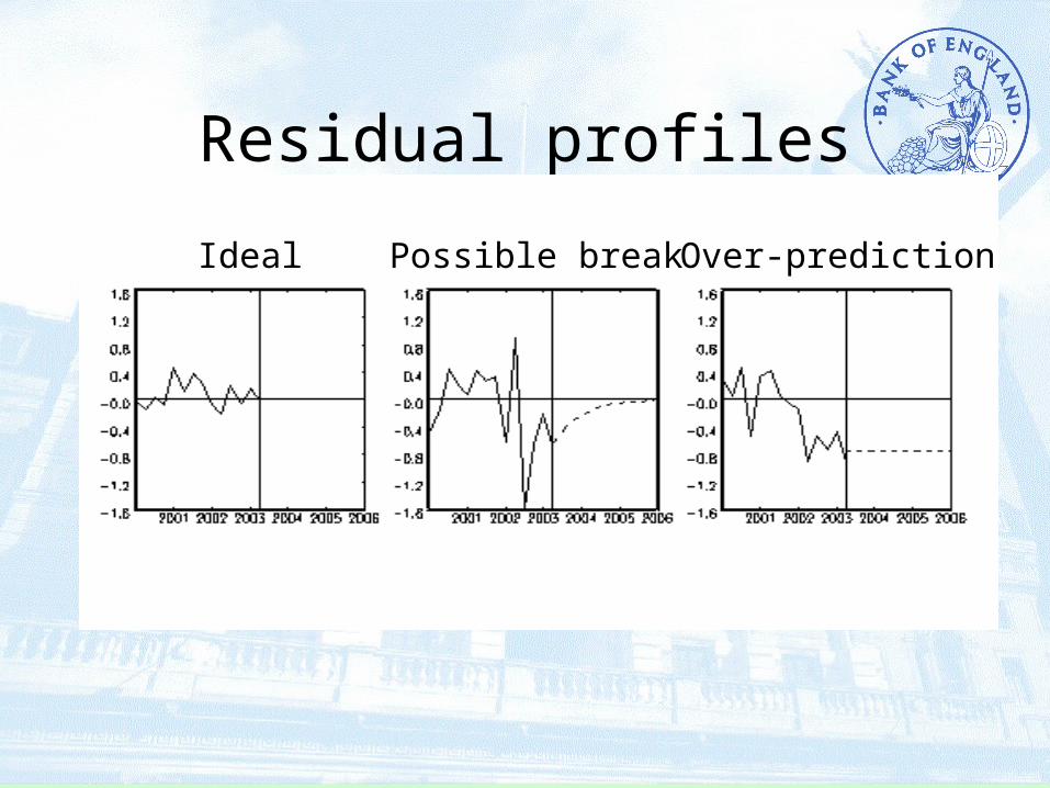
Residual profiles

Ideal Possible break Over-prediction

Evaluating the model forecast• Check performance of individual equations

– Implicit residuals a guide to how well equations track the recent past

– Forecast residuals may be averages of last one or two years, may fade back

• Alternate/revised equations– Models may have alternate equations, perhaps on a trial

basis – Equations may need to be re-estimated if data

sufficiently revised or latest data inconsistent

Evaluating the forecast (cont.)• Check assumptions

– Are the exogenous variables consistent with the forecast?

• i.e. are productivity trends consistent with growth

• Does the forecaster like the forecast?

• Does the MPC like the forecast?– Question of ownership

• Iterate

‘Week 2’

More news• For any lengthy forecast process will usually

need to incorporate additional data– More data on exogenous variables may be available

• Perhaps the world forecast updated

– Perhaps non-National Accounts data becomes available

• Price, wage and production indices

• Monthly data

– Financial market data needs updating

More news (cont.)• Impacts on:

– Exogenous variables– Adjustment/residual settings– Equation fit

• Do everything you did in Week 1 (again)

• Iterate– Incorporate new data– New or different judgments

‘Week n’

Finalise forecast• Agree on final numbers

• Assess impact of news

• Decide main risks to the forecast– Part of the whole forecast process: the

forecaster learns what drives the forecast– Scenario analysis– Perhaps present results using formal density

forecast or provide standard errors

Existing model,

existing data, old

forecast Final forecastNational accounts, other data

release

Run forecast on new data

Examine residuals,

re-estimate model, revise

assumptions

Other data releases (prices, exchange rates)

A ‘quarterly’ forecast round

Assumptions:exogenous, residuals,

define ragged edge

‘Issues’ meetings

Create database

Forecast evaluation

Scenario analysis,

risk assessment

‘Tuning’

Revise assumptions

Forecasting with rational expectations

• Models such as the new BEQM

• Expectations may be structurally important– Exchange rates – Consumption Euler equations, etc.

• Forecast values affect current behaviour– Any updates to path of exogenous variables

become news and affect ‘jump variables’– No news no jumps

Forecasting with rational expectations (cont.)

• How does the forecasting process change?– Variables ‘jump about’ more– Seemingly trivial changes have big effects– Residual adjustments need to be made much

more carefully• Future residuals affect current behaviour

– Up-to-the-minute data may incorporate the news already

• Jumps adjusted to where you are now

Forecasting with leading indicators

• Nothing essentially different– Indicator variables often available at different

frequency to main forecast– Used as alternative ‘satellite’ models

• Dynamic factor modeling(unobserved components)– Stock and Watson (2002)– Camba-Medez et al. (2001)

Forecast post mortem

• Part of the process is to see what went wrong– Informal judgement when the model is

deficient – Tests of forecast accuracy

• Diebold and Mariano (1995)

• Does the forecaster add value?

• Camba-Mendez, G. et al. (2001) ‘An Automatic Leading Indicator of Economic Activity: Forecasting GDP Growth for European Countries’, Econometrics Journal 4(1), S56-90.

• Clements, M.P and D. Hendry (1995) ‘Macro-economic Forecasting and Modelling’, Economic Journal 105(431), 1001-1013.

• Diebold, F.X and R. Mariano (1995) ‘Comparing Predictive Accuracy’, Journal of Business and Economic Statistics 13(3), 253-63

• Egginton, D., A. Pick and S.P. Vahey (2002) ‘‘Keep It Real!’: A Real-Time UK Macro Data Set’, Economics Letters 77(1), 15-22.

• Stock, J.H and M. Watson (2002) ‘Macroeconomic Forecasting Using Diffusion Indexes’, Journal of Business and Economic Statistics 20(2), 147-162