form and function in hillslope hydrology: characterization...

Hydrol. Earth Syst. Sci., 21, 3727–3748, 2017https://doi.org/10.5194/hess-21-3727-2017© Author(s) 2017. This work is distributed underthe Creative Commons Attribution 3.0 License.

Form and function in hillslope hydrology: characterization ofsubsurface flow based on response observationsLisa Angermann1,2, Conrad Jackisch3, Niklas Allroggen2, Matthias Sprenger4,5, Erwin Zehe3, Jens Tronicke2,Markus Weiler4, and Theresa Blume1

1Helmholtz Centre Potsdam, GFZ German Research Centre for Geosciences, Section Hydrology, Potsdam, Germany2University of Potsdam, Institute of Earth and Environmental Science, Potsdam, Germany3Karlsruhe Institute of Technology (KIT), Institute for Water and River Basin Management,Chair of Hydrology, Karlsruhe, Germany4University of Freiburg, Institute of Geo- and Environmental Natural Sciences, Chair of Hydrology, Freiburg, Germany5University of Aberdeen, School of Geosciences, Geography & Environment, Aberdeen, Scotland, UK

Correspondence to: Lisa Angermann ([email protected])

Received: 22 April 2016 – Discussion started: 10 May 2016Revised: 29 April 2017 – Accepted: 22 May 2017 – Published: 21 July 2017

Abstract. The phrase form and function was established inarchitecture and biology and refers to the idea that form andfunctionality are closely correlated, influence each other, andco-evolve. We suggest transferring this idea to hydrologicalsystems to separate and analyze their two main character-istics: their form, which is equivalent to the spatial struc-ture and static properties, and their function, equivalent tointernal responses and hydrological behavior. While this ap-proach is not particularly new to hydrological field research,we want to employ this concept to explicitly pursue thequestion of what information is most advantageous to un-derstand a hydrological system. We applied this concept tosubsurface flow within a hillslope, with a methodological fo-cus on function: we conducted observations during a natu-ral storm event and followed this with a hillslope-scale irri-gation experiment. The results are used to infer hydrologi-cal processes of the monitored system. Based on these find-ings, the explanatory power and conclusiveness of the dataare discussed. The measurements included basic hydrologi-cal monitoring methods, like piezometers, soil moisture, anddischarge measurements. These were accompanied by iso-tope sampling and a novel application of 2-D time-lapseGPR (ground-penetrating radar). The main finding regard-ing the processes in the hillslope was that preferential flowpaths were established quickly, despite unsaturated condi-tions. These flow paths also caused a detectable signal in thecatchment response following a natural rainfall event, show-

ing that these processes are relevant also at the catchmentscale. Thus, we conclude that response observations (dynam-ics and patterns, i.e., indicators of function) were well suitedto describing processes at the observational scale. Especiallythe use of 2-D time-lapse GPR measurements, providing de-tailed subsurface response patterns, as well as the combina-tion of stream-centered and hillslope-centered approaches,allowed us to link processes and put them in a larger con-text. Transfer to other scales beyond observational scale andgeneralizations, however, rely on the knowledge of structures(form) and remain speculative. The complementary approachwith a methodological focus on form (i.e., structure explo-ration) is presented and discussed in the companion paper byJackisch et al. (2017).

1 Introduction

Characterizing subsurface flow is the aim of many hydro-logical field and modeling studies. In hillslopes with steepslopes and structured soils, subsurface flow is controlled byhigh gradients and high heterogeneity of hydraulic proper-ties of the soil, resulting in a highly heterogeneous flow fieldand preferential flow paths (e.g., Scaini et al., 2017). Thespecific challenge of investigating preferential flow lies inits manifestation across scales, its high spatial variability,and pronounced temporal dynamics. A considerable number

Published by Copernicus Publications on behalf of the European Geosciences Union.

3728 L. Angermann et al.: Temporal dynamics of preferential flow

of experimental and model approaches have been proposedto investigate the issue (Beven and Germann, 1982, 2013;Šimunek et al., 2003; Gerke, 2006; Weiler and McDonnell,2007; Köhne et al., 2009; Germann, 2014). However, rapidflow in structured soils is still a challenge to current meansof observation, process understanding, and modeling.

In previous studies at the hillslope scale, the focus wasoften on lateral flow processes and the establishment of over-all connectivity. Hillslope-scale excavations yield informa-tion on spatial extent and characteristics of preferential flowpaths in 3-D (Anderson et al., 2009; Graham et al., 2010),but are highly destructive and lack the temporal compo-nent. Hillslope-scale tracer experiments in contrast resolvetemporal dynamics and velocities (Wienhofer et al., 2009;McGuire and McDonnell, 2010) but lack the spatial infor-mation. Hillslope-scale experiments are usually very laborintensive and require high technical effort, and most stud-ies are concentrated on well-monitored trenches (McGlynnet al., 2002; Tromp-Van Meerveld and McDonnell, 2006;Vogel et al., 2010; Zhao et al., 2013; Bachmair and Weiler,2012). Blume and van Meerveld (2015) give a thorough re-view of investigation techniques for subsurface connectivityand find experimental studies on this topic underrepresentedin hydrological field research.

In recent years, a trend towards non-invasive methodsfor hillslope-scale observations has emerged (Gerke et al.,2010), which has been an important improvement with re-gard to repeatability and spatial and temporal flexibility ofobservations (Beven and Germann, 2013). In this contextvarious geophysical methods have been applied for subsur-face exploration (e.g., Wenninger et al., 2008; Garré et al.,2013; Hübner et al., 2015). From all applied geophysicaltechniques ground-penetrating radar (GPR) is known as thetool providing the highest spatial and temporal resolution.GPR provides information on subsurface structures at mini-mal invasive cost (e.g., Lambot et al., 2008; Bradford et al.,2009; Jol, 2009; Schmelzbach et al., 2011, 2012; Steelmanet al., 2012). Its short measurement times and high sensitivitytowards soil moisture predestine GPR for monitoring subsur-face flow processes. Nevertheless, only few field studies existwhich have successfully applied surface-based GPR for theinvestigation of preferential flow paths or subsurface flow ingeneral (Truss et al., 2007; Haarder et al., 2011; Guo et al.,2014; Allroggen et al., 2015b). Previous GPR monitoringstudies rely on two different principles. The first approach re-lies on interpreting selected reflection surfaces and compar-ing this interpretation result between the individual recordedGPR surveys (Truss et al., 2007; Haarder et al., 2011). Theresult is a shift in GPR signal travel time, which can be inter-preted in terms of soil moisture changes, using a petrophysi-cal relation (e.g., the CRIM model, Allroggen et al., 2015b).The second approach relies on calculating difference imagesbetween individual GPR surveys (e.g., Birken and Versteeg,2000; Trinks et al., 2001; Guo et al., 2014; Allroggen andTronicke, 2015) and thereby highlighting areas of increased

changes in the subsurface. Due to the usually high noise levelof field data, such difference calculations are critical and re-quire sophisticated processing techniques (Guo et al., 2014;Allroggen and Tronicke, 2015).

Especially in structured soils, where subsurface flow islikely dominated by preferential flow paths, methods arerequired which are capable of covering the existing het-erogeneity. Point measurements and integrated observationsalone are barely able to meet this requirement. Structuralchanges of the subsurface as revealed by difference imagesobtained from GPR measurements, in contrast, reveal spa-tially discrete flow paths. We therefore applied and testedtime-lapse GPR measurements to investigate subsurface flowprocesses within a hillslope with shallow and highly struc-tured soils.

We chose a combination of conventional hydrologicalmethods and non-invasive GPR measurements to exploreflow processes by means of observations at the hillslope(hillslope-centered approach according to Blume and vanMeerveld, 2015). This hillslope-centered approach was sup-ported by stream-centered process observations, includinga basic hydrograph analysis and surface water stable iso-tope sampling during the natural rainfall event. Besides the2-D time-lapse GPR measurements, the hydrological meth-ods at the hillslope include surface runoff collectors, a densenetwork of soil moisture observation profiles, stable isotopesamples, and piezometers.

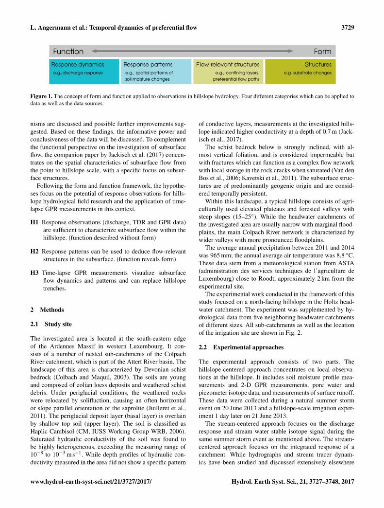
All methods and experimental results were subsumed un-der the framework of form and function as shown in Fig. 1.This framework was developed to analyze the explanatorypower of the different observations. The idea of the form andfunction dualism was established in architecture (form fol-lows function, Sullivan, 1896), is commonly used in biology(e.g., Thompson, 1942), and describes the link, mutual influ-ence, and co-evolution of the outer appearance and functionalpurpose of a (research) object.

In our case, form includes all static properties and spa-tial structures, such as topography, geology, and subsur-face structures, but also porosity, hydraulic conductivity, andstone content of the soil. Function summarizes all dynamicsand processes, including soil moisture dynamics, dischargebehavior, and preferential flow. These two are closely relatedand co-evolve. Based on this idea, Sivapalan (2005) sug-gested that patterns, responses, and functions are the basickey to understanding and describing a hydrological system,as they incorporate the morphogenetic processes that led tothe spatial structures. While this approach refers to the largerscale and the development of a general theory, our aim is toapply the form–function framework to observations at the lo-cal scale.

Starting on the left side of the spectrum presented in Fig. 1,we focus on the observation of response dynamics and re-sponse patterns. The potential of the methods for the inves-tigation of subsurface flow processes at the hillslope scaleand the characterization of typical runoff generation mecha-

Hydrol. Earth Syst. Sci., 21, 3727–3748, 2017 www.hydrol-earth-syst-sci.net/21/3727/2017/

L. Angermann et al.: Temporal dynamics of preferential flow 3729

R R F S

Figure 1. The concept of form and function applied to observations in hillslope hydrology. Four different categories which can be applied todata as well as the data sources.

nisms are discussed and possible further improvements sug-gested. Based on these findings, the informative power andconclusiveness of the data will be discussed. To complementthe functional perspective on the investigation of subsurfaceflow, the companion paper by Jackisch et al. (2017) concen-trates on the spatial characteristics of subsurface flow fromthe point to hillslope scale, with a specific focus on subsur-face structures.

Following the form and function framework, the hypothe-ses focus on the potential of response observations for hills-lope hydrological field research and the application of time-lapse GPR measurements in this context.

H1 Response observations (discharge, TDR and GPR data)are sufficient to characterize subsurface flow within thehillslope. (function described without form)

H2 Response patterns can be used to deduce flow-relevantstructures in the subsurface. (function reveals form)

H3 Time-lapse GPR measurements visualize subsurfaceflow dynamics and patterns and can replace hillslopetrenches.

2 Methods

2.1 Study site

The investigated area is located at the south-eastern edgeof the Ardennes Massif in western Luxembourg. It con-sists of a number of nested sub-catchments of the ColpachRiver catchment, which is part of the Attert River basin. Thelandscape of this area is characterized by Devonian schistbedrock (Colbach and Maquil, 2003). The soils are youngand composed of eolian loess deposits and weathered schistdebris. Under periglacial conditions, the weathered rockswere relocated by solifluction, causing an often horizontalor slope parallel orientation of the saprolite (Juilleret et al.,2011). The periglacial deposit layer (basal layer) is overlainby shallow top soil (upper layer). The soil is classified asHaplic Cambisol (CM, IUSS Working Group WRB, 2006).Saturated hydraulic conductivity of the soil was found tobe highly heterogeneous, exceeding the measuring range of10−8 to 10−3 ms−1. While depth profiles of hydraulic con-ductivity measured in the area did not show a specific pattern

of conductive layers, measurements at the investigated hills-lope indicated higher conductivity at a depth of 0.7 m (Jack-isch et al., 2017).

The schist bedrock below is strongly inclined, with al-most vertical foliation, and is considered impermeable butwith fractures which can function as a complex flow networkwith local storage in the rock cracks when saturated (Van denBos et al., 2006; Kavetski et al., 2011). The subsurface struc-tures are of predominantly geogenic origin and are consid-ered temporally persistent.

Within this landscape, a typical hillslope consists of agri-culturally used elevated plateaus and forested valleys withsteep slopes (15–25◦). While the headwater catchments ofthe investigated area are usually narrow with marginal flood-plains, the main Colpach River network is characterized bywider valleys with more pronounced floodplains.

The average annual precipitation between 2011 and 2014was 965 mm; the annual average air temperature was 8.8 ◦C.These data stem from a meteorological station from ASTA(administration des services techniques de l’agriculture deLuxembourg) close to Roodt, approximately 2 km from theexperimental site.

The experimental work conducted in the framework of thisstudy focused on a north-facing hillslope in the Holtz head-water catchment. The experiment was supplemented by hy-drological data from five neighboring headwater catchmentsof different sizes. All sub-catchments as well as the locationof the irrigation site are shown in Fig. 2.

2.2 Experimental approaches

The experimental approach consists of two parts. Thehillslope-centered approach concentrates on local observa-tions at the hillslope. It includes soil moisture profile mea-surements and 2-D GPR measurements, pore water andpiezometer isotope data, and measurements of surface runoff.These data were collected during a natural summer stormevent on 20 June 2013 and a hillslope-scale irrigation exper-iment 1 day later on 21 June 2013.

The stream-centered approach focuses on the dischargeresponse and stream water stable isotope signal during thesame summer storm event as mentioned above. The stream-centered approach focuses on the integrated response of acatchment. While hydrographs and stream tracer dynam-ics have been studied and discussed extensively elsewhere

www.hydrol-earth-syst-sci.net/21/3727/2017/ Hydrol. Earth Syst. Sci., 21, 3727–3748, 2017


Figure 2. Map of the investigated Colpach River catchment and thefour gauged sub-catchments. The site of the hillslope-scale irriga-tion experiment is located in the Holtz 2 catchment and is indicatedin red.

(Wrede et al., 2015; Martínez-Carreras et al., 2016, in thesame area), we wanted to use these data to position our hills-lope observation in the bigger picture of the catchment-scaledynamics. An overview of approaches, methods, and theirfoci is given in Fig. 3.

2.3 Stream-centered approach

The hydrological response behavior of several nested sub-catchments was investigated. At four locations v-notch ortrapezoidal gauges were installed and equipped with pres-sure transducers, measuring water level, electric conductiv-ity, and temperature (CTD sensors, Decagon Devices Inc.).Water levels were measured every 15 min. Precipitation wasmonitored with tipping buckets (Davis Instruments Corp.) inthe Holtz 1 headwater. All data were logged with CR1000data loggers (Campbell Scientific Inc.).

At the same locations and additionally close to the sourceof the Holtz River (Holtz 1 in Fig. 2), water samples weretaken with auto samplers (ISCO 3700, Teledyne). The bot-tles of the auto samplers were pre-filled with styrofoam beadsto avoid evaporation from the sample bottles. Samples werethen transferred to glass bottles and analyzed in the labo-

GPR patterns

GPR dynamicsSoil moisture dynamicsPiezometersPore water isotopesSurface runoff

GPR patternsSoil moisture profiles

Literature

Literature

Basic topography

Back

grou

ndIrr

igat

ion

Rain

eve

nt

Stream-centered Hillslope-centered

Response dynamics Response patterns Flow-relevant structures Structures

LiteraturePiezometer isotopesSurface water isotopesDischarge

Figure 3. Experimental methods applied in the stream-centered andhillslope-centered approaches, divided into the sampling during thenatural rain event and the irrigation experiment. Additionally, somestructural background information was obtained from the literatureand a digital elevation model.

ratory at the Chair of Hydrology, University of Freiburg.The isotopic composition (δ18O and δ2H) of the water sam-ples was measured by wavelength-scanned cavity ring-downspectrometry (Picarro L2120-iWS-CRDS). The results aregiven in δ-notation in ‰, describing the deviation of the ra-tio between heavy and light isotopes (2H/1H and 18O/16O)relative to the ratio of the Vienna Standard Mean Ocean Wa-ter (VSMOW). For liquid analysis the accuracy is given as0.1 ‰ for δ18O and 0.5 ‰ for δ2H (according to the manu-facturer).

In addition to the stream water, rainfall water was sam-pled. Bulk samples were collected during the rainfall eventsright next to the experimental site. The water from the satu-rated zone was manually sampled on a monthly basis over thecourse of 1 year from piezometers close to the sub-catchmentgauges. Samples were taken with a peristaltic pump fromfresh water flowing into the piezometers, after they had beenpumped empty (Fig. 2).

To calculate the event water contribution, we applied asimple hydrograph separation (Pearce et al., 1986). Equa-tion (1) shows the calculation of the discharge attributed tothe natural rain event Qe, based on the isotopic compositionof the base flow (cb) 3 days before the storm event, the riverwater during and after the event (ct), and the rain water (ce)(Leibundgut et al., 2011).Qt is the total discharge during and



●

●●●●●

●

●

●

●

●

●

●

●

●

● ●● ● ●

●

●

●

●

P

C

C

C

S

V(a)

(b)

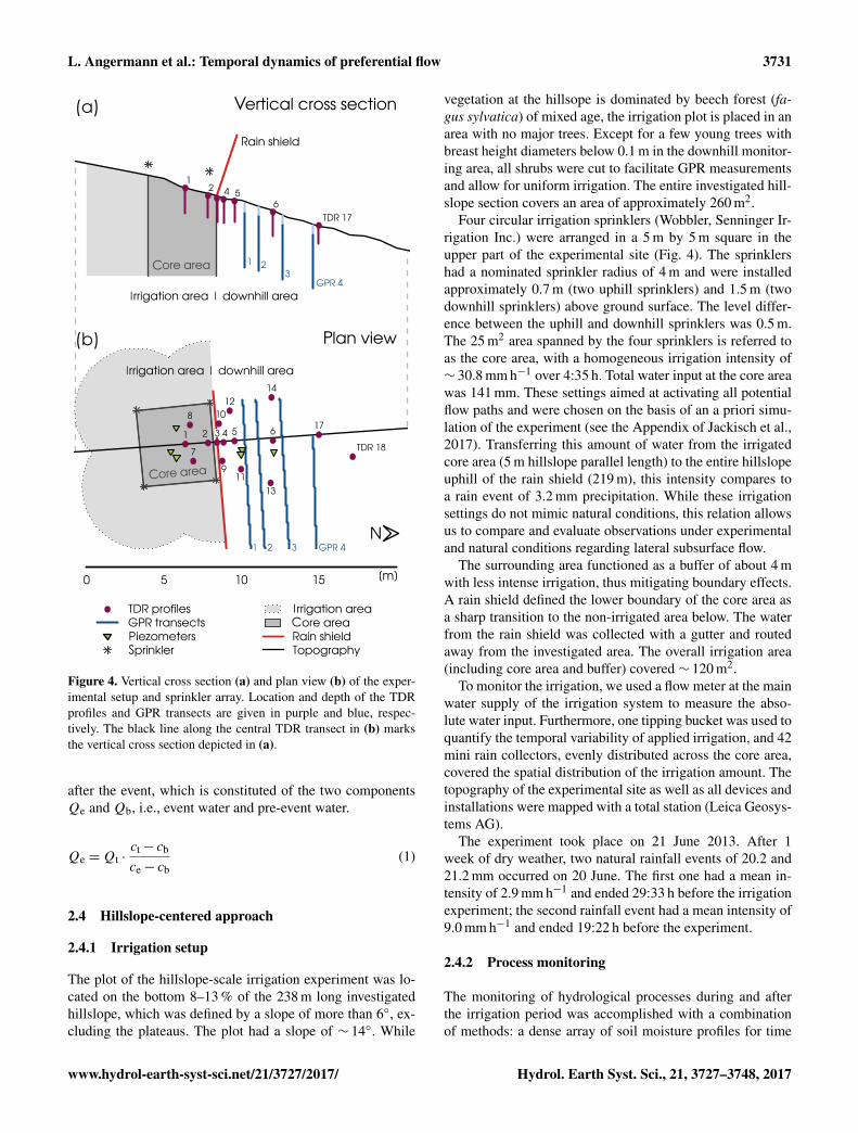
Figure 4. Vertical cross section (a) and plan view (b) of the exper-imental setup and sprinkler array. Location and depth of the TDRprofiles and GPR transects are given in purple and blue, respec-tively. The black line along the central TDR transect in (b) marksthe vertical cross section depicted in (a).

after the event, which is constituted of the two componentsQe and Qb, i.e., event water and pre-event water.

Qe =Qt ·ct− cb

ce− cb(1)

2.4 Hillslope-centered approach

2.4.1 Irrigation setup

The plot of the hillslope-scale irrigation experiment was lo-cated on the bottom 8–13 % of the 238 m long investigatedhillslope, which was defined by a slope of more than 6◦, ex-cluding the plateaus. The plot had a slope of ∼ 14◦. While

vegetation at the hillsope is dominated by beech forest (fa-gus sylvatica) of mixed age, the irrigation plot is placed in anarea with no major trees. Except for a few young trees withbreast height diameters below 0.1 m in the downhill monitor-ing area, all shrubs were cut to facilitate GPR measurementsand allow for uniform irrigation. The entire investigated hill-slope section covers an area of approximately 260 m2.

Four circular irrigation sprinklers (Wobbler, Senninger Ir-rigation Inc.) were arranged in a 5 m by 5 m square in theupper part of the experimental site (Fig. 4). The sprinklershad a nominated sprinkler radius of 4 m and were installedapproximately 0.7 m (two uphill sprinklers) and 1.5 m (twodownhill sprinklers) above ground surface. The level differ-ence between the uphill and downhill sprinklers was 0.5 m.The 25 m2 area spanned by the four sprinklers is referred toas the core area, with a homogeneous irrigation intensity of∼ 30.8 mm h−1 over 4:35 h. Total water input at the core areawas 141 mm. These settings aimed at activating all potentialflow paths and were chosen on the basis of an a priori simu-lation of the experiment (see the Appendix of Jackisch et al.,2017). Transferring this amount of water from the irrigatedcore area (5 m hillslope parallel length) to the entire hillslopeuphill of the rain shield (219 m), this intensity compares toa rain event of 3.2 mm precipitation. While these irrigationsettings do not mimic natural conditions, this relation allowsus to compare and evaluate observations under experimentaland natural conditions regarding lateral subsurface flow.

The surrounding area functioned as a buffer of about 4 mwith less intense irrigation, thus mitigating boundary effects.A rain shield defined the lower boundary of the core area asa sharp transition to the non-irrigated area below. The waterfrom the rain shield was collected with a gutter and routedaway from the investigated area. The overall irrigation area(including core area and buffer) covered ∼ 120 m2.

To monitor the irrigation, we used a flow meter at the mainwater supply of the irrigation system to measure the abso-lute water input. Furthermore, one tipping bucket was used toquantify the temporal variability of applied irrigation, and 42mini rain collectors, evenly distributed across the core area,covered the spatial distribution of the irrigation amount. Thetopography of the experimental site as well as all devices andinstallations were mapped with a total station (Leica Geosys-tems AG).

The experiment took place on 21 June 2013. After 1week of dry weather, two natural rainfall events of 20.2 and21.2 mm occurred on 20 June. The first one had a mean in-tensity of 2.9 mm h−1 and ended 29:33 h before the irrigationexperiment; the second rainfall event had a mean intensity of9.0 mm h−1 and ended 19:22 h before the experiment.

2.4.2 Process monitoring

The monitoring of hydrological processes during and afterthe irrigation period was accomplished with a combinationof methods: a dense array of soil moisture profiles for time



domain reflectrometric (TDR) measurements arranged as di-verting transects along the slope line, and four GPR transectslocated downhill of the core area and oriented parallel to thecontour lines and the rain shield for time-lapsed GPR mea-surements. The latter yielded vertical cross sections of thesubsurface.

A surface runoff collector was installed across 2 m at thelower boundary of the core area. Surface runoff was collectedby a plastic sheet installed approximately 1 cm below the in-terface between the litter layer and the Ah horizon of the soilprofile and routed to a tipping bucket.

An array of 16 access tubes for manual soil moisture mea-surement with TDR probes (Pico IPH, IMKO GmbH) cov-ered the depth down to 1.7 m below ground. The layout con-sisted of three diverging transects with four TDR profiles inthe lower half of the core area, the highest density of pro-files just downslope of the rain shield, and the furthest profileabout 9 m downhill (Fig. 4b). This setup allows for the sep-arate observation of predominantly vertical flow at the corearea and lateral flow processes at the downhill monitoringarea.

Soil moisture was measured manually. To increase thetemporal resolution of the measurements, three probes wereused in parallel. While these probes were identical with re-gard to measuring technique and manufacturing, they dif-fered slightly in sensor design: two TDR probes had an in-tegration depth (i.e., sensor head length) of 0.12 m, and oneprobe had an integration depth of 0.18 m. These sensors weremanually lowered to different depths into the 16 access tubes,where they measured the dielectric permittivity of the sur-rounding soil in the time domain through the access tubes.Given a mean penetration depth of 5.5 cm and a tube diame-ter of 4.2 cm, this yields an integration volume of ∼ 0.72 and1.05 L, respectively. The manual measurements were con-ducted in 0.1 m depth increments and followed a flexiblemeasuring routine with regard to the sequence in which theaccess tubes were measured. Thus, active profiles were cov-ered with higher frequency.

In addition to the hydrological methods, GPR was usedto monitor the shallow subsurface. Two-dimensional time-lapse GPR measurements were conducted along four tran-sects across the downhill monitoring area. The transects haddistances of ∼ 2, 3, 5, and 7 m to the lower boundary of thecore area and were arranged approximately perpendicularlyto the topographic gradient. Each transect was measured ninetimes. One measurement was taken before irrigation startedand the last one about 24:00 h after irrigation start.

The GPR system consisted of a pulseEKKO PRO acquisi-tion unit (Sensors and Software Inc.) equipped with shielded250 Mhz antennas. The data were recorded using a constantoffset of 0.38 m, a sampling interval of 0.2 ns, and a timewindow of 250 ns. For accurate positioning, a kinematic sur-vey strategy was employed. The positioning was based ona self-tracking total station (Leica Geosystems AG), whichrecorded the antenna coordinates as described by Boeniger

and Tronicke (2010). To guarantee the repeatability of the 2-D time-lapse GPR measurements, all four transects were de-fined by wooden guides for an exact repositioning of the an-tennas. The measurement of one transect took approximately2 min and measurements of all four transects were taken ev-ery 40–120 min during and after irrigation as well as 18:00and 24:00 h after irrigation start.

2.4.3 Isotope sampling

The stable isotope sampling included samples taken fromfive soil cores (pore water), piezometers (percolating porewater), as well as irrigation and rain water (input water). Thesoil cores were taken with a percussion drill with a head di-ameter of 7 cm and split into 5 cm increments to get depthprofiles of the stable isotopic composition (δ18O and δ2H) ofthe pore water. Two profiles were taken before the rainfallevents, one after the first minor rain event on 20 June, andtwo more after the irrigation experiment (at the core area andthe downhill monitoring area). All profiles covered a depthof ∼ 1.7 m below ground.

At the locations of the pre-irrigation soil cores, piezome-ters were installed. Additionally, three more piezometerswere installed at a depth of ∼ 1.0 m. This depth was chosenbased on observations in the core samples, which showed wetareas at the depths between 0.8 and 1.2 m, right above the Cvhorizon. All piezometers consist of PVC tubes of 5 cm di-ameter and were screened at the bottom 20 cm. They wereequipped with pressure transducers (CTD sensors, DecagonDevices Inc.). As only a few mL of water were seeping intothe piezometers, water tables could not be properly moni-tored, and the data will not be shown. However, the watercould be sampled using a peristaltic pump. In addition to thepore water and piezometer samples, bulk samples of rain-fall water were collected during the rainfall events prior tothe irrigation experiment and directly next to the irrigationplot. Water samples were also taken from the irrigation waterreservoir five times during irrigation.

The soil samples were prepared following the direct equi-libration method as proposed by Wassenaar et al. (2008) anddescribed in detail by Sprenger et al. (2016). The precisionfor the method is reported to be 0.31 ‰ for δ18O and 1.16 ‰for δ2H (Sprenger et al., 2015). All water samples were ana-lyzed following the same procedure as described in Sect. 2.3.

2.5 Data analysis

2.5.1 TDR data analysis

Almost 5000 individual soil moisture measurements weretaken during the irrigation experiment. As the three TDRprobes had different integration depths (0.12 and 0.18 m),the measurements had a different depth offset relative to theground surface when referenced to the center of the probe,and had to be aligned. To do so, the measurements, which



were originally taken in 0.1 m increments, were resampled atdepths by linear interpolation. Due to the potentially shortcorrelation length of soil moisture (Zehe et al., 2010), in-verse distance interpolation between two locations is gener-ally not appropriate. In the case of the vertical profiles, how-ever, the integration depths of the probes exceeded the mea-suring increments. Due to the resulting overlap of the inte-gration volumes, this procedure was assumed to be adequate.The measurement of one depth increment took between ap-proximately 10 and 30 s. While the data were interpolatedin time for better visualization, all data analyses were per-formed with the uninterpolated data.

All TDR measurements were referenced to the last mea-surement before irrigation. The resulting data set of rela-tive soil moisture changes 1θ was used for the discussionof soil moisture dynamics and response velocity calculation(Sect. 2.5.4). The storage changes (mm) in the top 1.4 m ofthe core area were estimated based on the four core area TDRprofiles TDR1, TDR2, TDR7, and TDR8, by multiplying the1θ (%) of each depth increment by the respective depth in-terval (mm). Together with the time series of water input,these data were used to estimate the mass balance dynamicsof the core area.

2.5.2 Data processing of 2-D time-lapse GPRmeasurements

The time-lapse GPR survey comprised repeated recordingsof vertical 2-D GPR data along the four transects. The dataprocessing of each measurement relied on a standard pro-cessing scheme, including bandpass filtering, zero time cor-rection, exponential amplitude preserving scaling, inline fk-filtering, and a topographic migration approach, as presentedby Allroggen et al. (2015a). The GPR data were analyzedusing an appropriate constant velocity and gridded to a 2-Dtransect with a regular trace-spacing of 0.02 m.

There is no standard interpretation procedure for the anal-ysis of time-lapse GPR data. Most approaches are based oncalculating trace-to-trace differences (Birken and Versteeg,2000; Trinks et al., 2001) or picking and comparing selectedreflection events in the individual time-lapse transects (All-roggen et al., 2015b; Haarder et al., 2011; Truss et al., 2007).In the context of this study, however, both approaches pro-vided only limited interpretable information. Considering themethodological uncertainty, the highly heterogeneous soildid not provide reflectors which were a suitable reference.Therefore, we used a time-lapse structural similarity attributepresented by Allroggen and Tronicke (2015), which is basedon the structural similarity index known from image pro-cessing (Wang et al., 2004). This approach incorporates acorrelation-based attribute for highlighting differences be-tween individual GPR transects and has been shown to im-prove imaging, especially for noise data and limited surveyrepeatability.

The calculated structural similarity attributes are a qualita-tive indicator of relative deviations from the reference state.The GPR data indicated remaining water from the naturalrain event when the experiment was started. Therefore, thelast acquisition time 24:00 h after irrigation start was cho-sen as the reference time for all GPR transects. Based on theassumption that the reference state is the one with the low-est water content, decreasing structural similarity was inter-preted as an increase in soil moisture.

To convert GPR two-way travel time (TWT) into depth,we used the average measured GPR propagation velocity of0.07 m ns−1. This velocity is based on additional commonmidpoint data and the assumption of static conditions dur-ing the experiment. Using this velocity, the GPR transectscovered a TWT of 120 ns, which corresponds to a depth of∼ 4.2 m below ground surface. Approximately the first 20 nsof each transect are influenced by the interfering arrival ofthe direct wave and the ground wave. Consequently, we ob-serve no interpretable reflected energy in the uppermost timewindow. Thus, the 2-D GPR measurements imaged the sub-surface between ∼ 0.7 and 4.2 m depth below ground.

2.5.3 Comparison of a natural event vs. irrigationbased on 2-D GPR data

To interpret the structural similarity attribute images, we dis-criminated between the signal of the natural rain event andthe irrigation. The discrimination was based on the tempo-ral dynamics of each pixel of the GPR transects (i.e., everysingle value in the matrix of distance along the GPR transectand depth/TWT). The first GPR measurements were taken12:52 h after the end of the second rainfall event (i.e., 6:30 hbefore irrigation start) and the observed responses were at-tributed to the natural rain event. Once the structural similar-ity attribute value of a pixel decreased more than 0.15 afterirrigation start, the signal of that pixel was attributed to the ir-rigation. The threshold of 0.15 was chosen based on the noiseof the last measurement 18:00 h after irrigation start and ex-ceeds the standard deviation of that measurement by a factorof 3. The same procedure was applied to infer the time of firstresponse to the irrigation signal, which was used to calculateresponse velocities.

This procedure yields 2-D maps of response patterns, witheach pixel being attributed to either the irrigation or the nat-ural rain event. The structural similarity values are a semi-quantitative measure of soil moisture and thus no reliableindicator to directly compare actual soil moisture responsesrecorded at different locations or at different times. We there-fore used the areal share of the monitored cross sections tocompare the impact of the two input events. To do so, all pix-els of one of the two categories (natural rainfall or irrigation)which fell below the value of 0.85 (i.e., maximum similar-ity 1 minus threshold 0.15) were counted and expressed as afraction of the entire cross section. The resulting areal sharedoes not represent the actual share of activated flow paths,



but is a semi-quantitative indicator of the hillslope cross sec-tion impacted by active flow paths.

2.5.4 Response velocity calculation

As no tracers were used for irrigation, dynamic processes hadto be inferred from changes in state. For TDR measurements,the time of first response was defined as an increase in soilmoisture by 2 % vol relative to initial conditions. This thresh-old was chosen based on the standard deviation of measure-ments under presumably constant conditions. The time offirst response was identified for each TDR profile and depthincrement.

Due to the experimental setup, soil moisture dynamics onthe core area were dominated by vertical processes, while lat-eral processes controlled the dynamics at the downhill moni-toring area. Accordingly, vertical and lateral response veloc-ities were calculated from core area and downhill monitoringarea TDR profiles, respectively.

As a continuous wetting of the soil profile could not beassumed, all response velocities were calculated for the en-tire depth (or distance) instead of depth increments. Re-sponse velocities are therefore integrated values describingprocesses in the entire soil column above. This procedurealso accounts for heterogeneous processes and preferentialflow paths, which may bypass shallower depths without leav-ing a detectable soil moisture signal.

Lateral response velocities account for the depth and dis-tance between soil surface at the rain shield and TDR profilein question and, therefore, integrate lateral and vertical flow.They were calculated for every depth of the soil moistureprofiles at the downhill monitoring area. The time of the veryfirst response signal measured on the core area was used asreference time t0, which was 15 min after irrigation start. Dueto the slope-parallel or horizontal orientation of the sapro-lite, we assumed that the water flows either vertically or lat-erally rather than diagonally. Based on this assumption, thedistances were calculated from the slope parallel distance ofeach profile from the lower boundary of the core area plusthe depth of every measuring point. The distance assump-tions for both, vertical and lateral velocity calculations, donot resolve tortuosity of flow paths and, therefore, drasticallyreduce the complexity of the flow path network to its inte-gral behavior. The calculated response velocities are thus notto be interpreted as in situ flow velocities in the flow paths,but rather as the minimum necessary velocity explaining theobserved arrival of the wetting signal.

The same holds true for the lateral response velocities cal-culated from GPR data. In accordance with the separation ofthe natural rain event signal and the irrigation signal, the firstdecrease in structural similarity of more than 0.15 was inter-preted as the arrival of the irrigation signal. Single structuresand flow paths are not the focus of this article and will bediscussed in the companion study by Jackisch et al. (2017).Here, we therefore simplified the 2-D patterns to a depth dis-

tribution of occurring response velocities. To do so, all areasthat were newly activated at the time of one measurementwere accumulated by depth and given as a portion of the en-tire width of each GPR transect. Comparable to the proce-dure applied to the TDR data, the response velocities werethen calculated from the respective measuring time, the dis-tance between transect and irrigation area, and the depth. Theresulting patterns show the spatial fraction of the depth in-crement which is connected to flow paths of the calculatedvelocity or faster and give an idea of the spatial distributionof the GPR response velocities.

3 Results

3.1 Response to the natural rainfall

3.1.1 Stream-centered approach: hydrograph andsurface water isotopes

In response to the summer storm event just beforethe hillslope-scale irrigation experiment, all gauged sub-catchments showed double-peak hydrographs, with one im-mediate short peak, and one prolonged peak delayed by sev-eral hours (second rainfall event, Fig. 5). In the headwa-ter catchments (Holtz 2, Weierbach 1 and 2), the first peakoccurred almost instantly, while the more distant Colpachgauge showed a delay of approximately 3:00 h. The secondresponse was prolonged, with a maximum approximately36:00 h after the event. The strength and ratio of the twopeaks varied across different sub-catchments and accordingto hydrological conditions, but the general pattern is char-acteristic of the hydrological behavior of the Colpach Rivercatchment. Similar behavior was also reported by Feniciaet al. (2014), Wrede et al. (2015), and Martínez-Carreraset al. (2016), whose investigations focused on the Weier-bach 1 catchment.

A simple mass balance calculation revealed that the firstpeak constituted 7.5 % of the total event runoff at gaugeHoltz 2. The total event runoff coefficient was 0.44. Refer-enced to the precipitation amount, about 3.3 % of the inputleft the headwater within 7:00 h after the rain event (Table 1).In the neighboring Weierbach catchment and the Colpach,the first peak contributed more strongly to the total eventrunoff (14.2 and 12.9 % at Weierbach 1 and 2, and 19.7 %at Colpach, Table 1).

The δ18O signature of the stream water is indicative ofthe origin of the water. It showed strong dynamics dur-ing the discharge response to the rain events on 20 June(Fig. 5). The results of the hydrograph separation show thatthe event water contributed up to 67.6 % to the event runoffduring the response to the first rain event in the morningof 20 June (Colpach, 6:00 h). After that, the total dischargedropped again, with the event water contribution decreasingto 31.6 %. With the onset of the first peak caused by the sec-



-1

S

WP

P

TD

P -1

Figure 5. The figure shows the natural storm event on 20 June 2013 in the Colpach River catchment and the local intensity of the irrigationon 21 June 2013. The hydrographs below show the discharge response of four nested catchments (solid lines), in combination with thedynamics of the δ18O isotopic composition of the surface water (dots). The isotopic composition of the groundwater (annual mean) andthe precipitation (daily values) are given by the dashed lines. Furthermore, the dynamic response of the GPR signal to natural and artificialrainfall is given in green and blue. While the first minor rain event caused only a weak response, the second event caused a double-peakdischarge response in all sub-catchments. The irrigation experiment took place 19:22 h after the rain event.

ond rain event at 19:20 h, the event water contribution in-creased again and reached values of over 50 % (58.0 % in theColpach at 22:00 h, 55.2 % in the Holtz 1 catchment, 21:51 hon 20 June; Fig. 5). δ18O values then declined, indicatingevent water contributions of around 20.0 % (24.8 % at 4:00 hin the Colpach, 18.1 % at 13:03 h in Holtz 2, and 16.2 % at21:28 h in Holtz 1 on 21 June). Weierbach 1 and 2 showedthe same pattern, with event water contributions well above50.0 % for the first peak of the second rainfall event.

Uncertainty in hydrograph separation was caused by theuncertainty of the stable isotopic composition of the precipi-tation input. The uncertainty due to spatial variability of theprecipitation input was kept minimal for Holtz 2, by sam-pling the precipitation within the small catchment (45.9 ha).While we could not sample the isotopic input at high tempo-ral frequency, the bulk sample of the precipitation data rep-resents a weighted average of the input isotopic signal.

3.1.2 Hillslope-centered approach: subsurface responsepatterns

The 2-D time-lapse GPR measurements yield images ofstructural similarity referenced to the last measurement,which were taken 24:00 h after irrigation start, which trans-lates to 43:22 h after the second natural rain event. The first

GPR measurements were taken about 12:52 h after the sec-ond rain event and can be interpreted as the subsurface re-sponse patterns of this event (Fig. 6a). The subsequent GPRmeasurements furthermore show the temporal dynamics ofthe rainfall signal, overlain by the irrigation signal. The highinitial signals, as well as the high but decreasing areal shareof active regions in all transects during the first measure-ments until 1:30 h after irrigation start (Fig. 6b), indicatedfree water remaining from the preceding natural rain eventwhich slowly disappeared.

While transect 1 showed only a weak signal of the natu-ral event in the first measurement, transects 2 and 3 exhib-ited stronger and longer lasting signals. The areal share ofactive regions of the four transects in the measurement pre-ceding the irrigation experiment was 38.5, 51.6, 64.4, and50.5 % from upslope to downslope. Except for transect 2,which even showed a slight increase in the areal share of ac-tive regions between the first and second measurements, thesignal of the natural rain event was continuously vanishing(Fig. 6b).



(a)

(b) T

RD

A

T

FN

N

S

L

Figure 6. (a) Two-dimensional GPR data showing the subsurface response patterns caused by the natural rainfall event. The data show thestructural similarity between the first GPR measurement (approximately 6:30 h before irrigation start and 12:52 h after the second rainfallevent) and the last one. Low values of structural similarity are interpreted as high changes in soil moisture. (b) Temporal dynamics of theareal share of active regions attributed to the natural rain event and the irrigation. Activated regions were identified by a structural similarityattribute of less than 0.85. Data were interpolated linearly between the measurements for visualization. The measurements shown in (a) showthe data used to calculate the first data point shown in (b).

3.2 Hillslope-scale irrigation experiment

3.2.1 Core area water balance dynamics

The irrigation intensity was relatively constant over time,with only weak fluctuations due to gradual clogging of theintake filter. The spatial distribution of the irrigation inten-sity on the core area was influenced by the sprinkler setupand the slope of the experimental site. The mean intensityon the core area was 30.8± 73 mm h−1, with slightly highervalues in the vicinity of the four sprinklers. Surface runoffat the lower boundary of the core area started 20 min afterirrigation start and ceased with the same time lag. In total,surface runoff amounted to 0.5 L, which equals only 0.02 %of the water balance.

The core area mass balance is shown in Fig. 7, depictingthe storage increase in the top 1.4 m of the soil. All profilesshowed a mass recovery of more than 100 % (i.e., higher stor-age increase than water input at measuring time; see Fig. 7)in the first 60 min of the irrigation period. In profiles TDR1,TDR2, and TDR8 mass recovery then decreased and droppedbelow 100 %, while TDR7 increased further, with a maxi-mum overshoot of almost 50 % approximately 2:00 h afterirrigation start. The last measurement during irrigation wastaken approximately 50 min before the end of the irrigationperiod. At this time, the average storage increase was morethan 20 % lower than the input mass.

●

●

●●

● ●

●

●

●

● ●

●

●

●

● ●

●

●

●

●●

●

●

●

●

●

●

●

●

●●

●

● ●

●

●●

●

● ●

●

●

●

●

W

W

Figure 7. Water balance of the top 1.4 m of the soil column forthe four core area TDR profiles. Dashed lines indicate the storageincrease at the last measurement before irrigation ended. The vari-ability between the four profiles shows the high heterogeneity andcauses uncertainty regarding the average mass balance of the corearea.

The first measurement after irrigation (6–19 min after irri-gation stopped) showed a mean deficit of 54.7 %, indicatingthat on average 31.2 % (between 18.6 and 43.9 %) of the wa-ter that has been recorded at the last measurements beforeirrigation stop was freely percolating and had left the mon-itored depth immediately. After this fast instantaneous reac-tion, the water content decreased equably. Mean total massrecovery dropped to 8.9 % after 18:24 h after irrigation start



●

●

●

●

● ●

●●●

●

● ●

●

TTT

D

D

D

D

D

D

S

MP

C

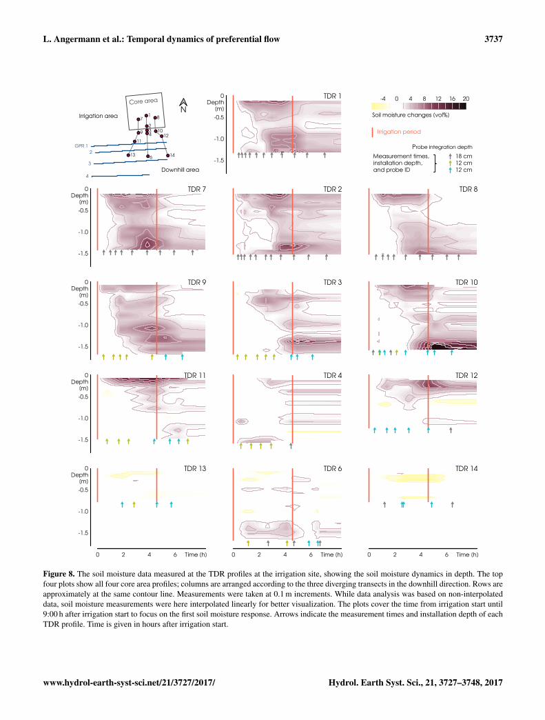
Figure 8. The soil moisture data measured at the TDR profiles at the irrigation site, showing the soil moisture dynamics in depth. The topfour plots show all four core area profiles; columns are arranged according to the three diverging transects in the downhill direction. Rows areapproximately at the same contour line. Measurements were taken at 0.1 m increments. While data analysis was based on non-interpolateddata, soil moisture measurements were here interpolated linearly for better visualization. The plots cover the time from irrigation start until9:00 h after irrigation start to focus on the first soil moisture response. Arrows indicate the measurement times and installation depth of eachTDR profile. Time is given in hours after irrigation start.



and almost returned to initial conditions (1.6 %) after 24:00 hafter irrigation start.

3.2.2 Soil moisture profiles and dynamics

The high variability in soil moisture dynamics observed inthe TDR profiles is summarized in Fig. 8. The four upper-most panels (rows 1 and 2) show the core area profiles.Columns represent the three diverging TDR transects. Thegeneral pattern observed at the core area was characterizedby a strong and comparably fast response in the top 0.4 m ofthe soil and below the depths of approximately 1.2 m. The re-sponse in between these active layers was more diverse andgenerally weaker.

Soil moisture in the top 0.4 m of the soil of TDR1, TDR7,and TDR8 quickly stabilized around constant values, indicat-ing the establishment of quasi steady-state conditions. Afterthe end of the irrigation, the soil moisture quickly declineddown to a 1θ of 4 % vol, indicating a very fast response tothe dynamics of the water input. In contrast to the fast es-tablishment of steady-state conditions and the fast decline, aslightly increased water content of up to 4 % vol above ini-tial conditions was persistent in distinct depth increments andwas also measured even 24:00 h after irrigation stopped.

The soil moisture patterns at the downhill monitoring areawere more diverse. Profiles located directly below the rainshield (TDR9, TDR3, and TDR10 with a distance to corearea of 0.2–0.5 m, Fig. 8) exhibited dynamics that resem-ble the reaction at the core area, but with mostly lower in-tensities and higher variability in depth. More distant TDRprofiles however showed a highly variable picture. Distinctlayers in variable depths were activated, while no change inthe water content was seen at the other soil depths. Espe-cially noteworthy are TDR10 and TDR11, which showed astrong soil moisture increase of up to 18 % vol below 1.4 mdepth and around 10 % vol in the top 0.3 m of the soil. Pro-files TDR13, TDR6, and TDR14 showed only weak signals,with the strongest response below 1.4 m below ground inTDR6. Profiles TDR6, TDR12, TDR13, and TDR14 showedthe strongest decrease in soil moisture over the course of themeasurements, with 1θ of −3.7, −4.4, −5.8, and −6.2 %vol at certain depths, indicating vanishing free water from thestorm event. While the results from the left (TDR7, TDR9,and TDR11) and right (TDR8, TDR10, and TDR12; seeFig. 8) transects suggested lateral flow at different depths,the central transect (TDR1 through TDR6) did not indicatelateral flow.

3.2.3 Time-lapse GPR dynamics

The TDR measurements at the downhill monitoring areawere complemented by the 2-D time-lapse GPR measure-ments (see Fig. 4), yielding 2-D images of structural similar-ity attributes referenced to the last measurement 24:00 h afterirrigation start (Fig. 9). The first irrigation signals (shown in

blue in Fig. 9) appeared in the first measurement after irri-gation start (1:28 h), with transect 1 showing the clearest re-sponse. After about 3:23 h strong, localized signals occurredand increased in intensity over time. The general maximumwas reached approximately 5:18 h after irrigation start, show-ing distinct activated flow paths. Most signals started to de-cline after 6:45 h, which is 2:10 h after the end of the irriga-tion period.

In transect 2 some weak signals appeared at the depth be-low 2.5 m 1:30 h after irrigation start. At this time, the signalwas close to the noise level, but the pattern became strongerand more distinct in the following measurements. At tran-sect 3, the persisting signal of the natural rain event made itdifficult to identify the irrigation-induced response. However,a weak irrigation signal appeared after 1:28 h and reachedits maximum at 6:45 h after irrigation start. At transect 4the structural similarity attribute values were generally low,which indicates a low deviation from the reference state. Ei-ther the mobile water showed low dynamics (with regard tototal mass over time) or water was less confined to specificstructures and local changes are less pronounced. Both inter-pretations suggest that this transect was generally wetter dueto its proximity to the river. Overall, the experiment does notappear to have affected this transect much.

The overview of all GPR measurements in Figs. 6b and 9visualizes the dynamics of the hillslope section. The greennatural rainfall signal faded from uphill to downhill, with thehighest intensity and duration in transect 3. After irrigationstart, the blue irrigation signal appeared, gradually propagat-ing downhill and eventually overpowering the natural rainsignal; 18:00 h after irrigation start (i.e., 13:25 h after irriga-tion ended), no changes in the GPR signal could be observedanymore. This suggests steady soil moisture conditions and,thus, the absence of highly mobile water in all transects. Themobile water either left the monitored area or dispersed bydiffusion into the matrix surrounding preferential flow paths,where it remained beyond the time of the reference measure-ment and thus would not have been visible by means of struc-tural similarity attributes.

3.2.4 Pore water and piezometer isotope responses

The temporal dynamics of the stable isotope compositions ofthe pore water (selected depths shown as circles in Fig. 10a)partially traced the signals of the rainfall and irrigation waterinput (green lines and blue triangles). The high δ2H signalof the first minor rainfall event (dark green) was clearly vis-ible in the top 10 cm below ground in the profile sampled atthe downhill monitoring area 24:00 h before irrigation and5:30 h after this rainfall event (Fig. 10a and c). Similarly, theisotope signal of the second rainfall event (light green) andthe irrigation water (blue triangles) could be seen in the top10 cm of the soil at the core area and the downhill monitor-ing area, respectively. Especially the isotope profile taken atthe core area after irrigation showed an increase in δ2H in the



L

E

T

M

SPI

Figure 9. Structural similarity attributes calculated from time-lapse GPR data. All measurements were referenced to the last one 24:00 hafter irrigation start, indicating changes in the GPR reflection patterns associated with soil moisture changes. A structural similarity attributevalue of 1 indicates full similarity; lower values signify higher deviation from the reference state. Water from the preceding natural rain event(green) was identified by constant or increasing structural similarity attributes. Water from the experimental irrigation (blue) was identifiedby decreasing values after irrigation start by more than 0.15. Within one column the rows give a sequence over time (after irrigation start).Columns proceed downhill, with increasing distance from the rain shield.



Figure 10. Stable isotope data from precipitation, irrigation, piezometers, and pore water samples. (a) Temporal dynamics of pore water andpiezometer δ2H in relation to water input by precipitation (bulk samples) and irrigation. Pore water data are shown only for the depths ofpiezometer filters (compare with panels (b) and (c) for depths) and the top soil (0.1 m below ground). The graph shows the direct impactof the water input (dashed lines) on the pore water isotope composition of the top soil. (b, c) Pore water and piezometer data over depths,separated by core area and monitoring area. Water input stable isotope data are indicated at the soil surface.

top 0.85 m below ground, showing the influence of both, theirrigation and the event water. Below the depth of approx-imately 1.2 m of all profiles, the soil water isotope compo-sition seemed not to be impacted by the rainfall events andirrigation.

Only a few mL of water were seeping into the piezometers,with piezometer B being the only one that could be sampledmore than once. Piezometer B was sampled first shortly afterthe irrigation ended (0:20 h) and showed a composition thatwas close to the irrigation water. The other two samples 1:32and 13:38 h after irrigation ended showed a decrease in δ2H,towards the composition of the soil water (red and orangediamonds in Fig. 10).

Piezometers A, C, G, and H were sampled once 13:38 hafter irrigation ended. The water sampled from piezometersat the core area (A and C, pink diamonds) showed the samecomposition as the irrigation water. Piezometers located atthe downhill monitoring area (G and H, purple diamonds) incontrast showed an isotopic composition similar to the rain-fall water and different to the pore water in the depth profiles.

3.2.5 Response velocities

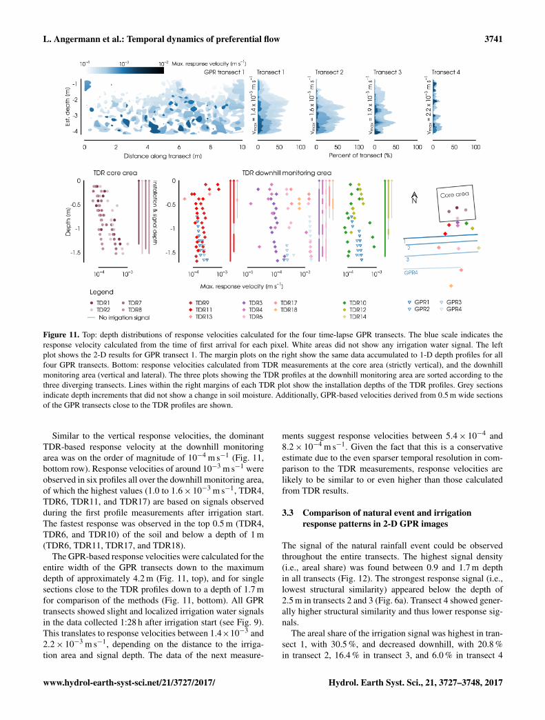
The results of the calculated response velocities from TDRand GPR measurements are summarized in Fig. 11. The toprow shows the depth distribution of observed response ve-locities for all GPR transects. The bottom row shows theTDR-based results, separated into core area profiles and thethree diverging transects. In addition to the TDR-based re-sponse velocities, GPR-based velocities observed in 0.5 mwide sections of the GPR transects which were closest to thedisplayed TDR profiles are shown in the plot.

At the core area, the dominating vertical response velocitywas around 10−4 m s−1, with a tendency to increasing veloc-ities with depth (Fig. 11, bottom left). As response velocitieswere calculated for the entire soil profile above the measuringdepth, this increase indicates a bypass of intermediate depthsthrough preferential flow paths, and a limited and slow inter-action with the matrix. The highest observed vertical velocitywas 10−3 m s−1 at the depth of 1.4 m below ground. The re-spective soil moisture signal was recorded in the very firstmeasurement after irrigation start, which indicates that wemight have even missed the first response.



Figure 11. Top: depth distributions of response velocities calculated for the four time-lapse GPR transects. The blue scale indicates theresponse velocity calculated from the time of first arrival for each pixel. White areas did not show any irrigation water signal. The leftplot shows the 2-D results for GPR transect 1. The margin plots on the right show the same data accumulated to 1-D depth profiles for allfour GPR transects. Bottom: response velocities calculated from TDR measurements at the core area (strictly vertical), and the downhillmonitoring area (vertical and lateral). The three plots showing the TDR profiles at the downhill monitoring area are sorted according to thethree diverging transects. Lines within the right margins of each TDR plot show the installation depths of the TDR profiles. Grey sectionsindicate depth increments that did not show a change in soil moisture. Additionally, GPR-based velocities derived from 0.5 m wide sectionsof the GPR transects close to the TDR profiles are shown.

Similar to the vertical response velocities, the dominantTDR-based response velocity at the downhill monitoringarea was on the order of magnitude of 10−4 m s−1 (Fig. 11,bottom row). Response velocities of around 10−3 m s−1 wereobserved in six profiles all over the downhill monitoring area,of which the highest values (1.0 to 1.6× 10−3 m s−1, TDR4,TDR6, TDR11, and TDR17) are based on signals observedduring the first profile measurements after irrigation start.The fastest response was observed in the top 0.5 m (TDR4,TDR6, and TDR10) of the soil and below a depth of 1 m(TDR6, TDR11, TDR17, and TDR18).

The GPR-based response velocities were calculated for theentire width of the GPR transects down to the maximumdepth of approximately 4.2 m (Fig. 11, top), and for singlesections close to the TDR profiles down to a depth of 1.7 mfor comparison of the methods (Fig. 11, bottom). All GPRtransects showed slight and localized irrigation water signalsin the data collected 1:28 h after irrigation start (see Fig. 9).This translates to response velocities between 1.4×10−3 and2.2× 10−3 m s−1, depending on the distance to the irriga-tion area and signal depth. The data of the next measure-

ments suggest response velocities between 5.4× 10−4 and8.2× 10−4 m s−1. Given the fact that this is a conservativeestimate due to the even sparser temporal resolution in com-parison to the TDR measurements, response velocities arelikely to be similar to or even higher than those calculatedfrom TDR results.

3.3 Comparison of natural event and irrigationresponse patterns in 2-D GPR images

The signal of the natural rainfall event could be observedthroughout the entire transects. The highest signal density(i.e., areal share) was found between 0.9 and 1.7 m depthin all transects (Fig. 12). The strongest response signal (i.e.,lowest structural similarity) appeared below the depth of2.5 m in transects 2 and 3 (Fig. 6a). Transect 4 showed gener-ally higher structural similarity and thus lower response sig-nals.

The areal share of the irrigation signal was highest in tran-sect 1, with 30.5 %, and decreased downhill, with 20.8 %in transect 2, 16.4 % in transect 3, and 6.0 % in transect 4



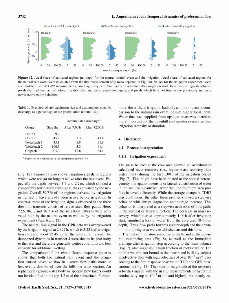
Figure 12. Areal share of activated regions per depth for the natural rainfall event and the irrigation. Areal share of activated regions forthe natural rain event were calculated from the first measurement only (also depicted in Fig. 6a). Values for the irrigation experiment wereaccumulated over all GPR measurements, counting every pixel that had been activated after irrigation start. Here, we distinguish betweenpixels that had been active before irrigation start and were re-activated again, and pixels which have not been active previously and werenewly activated by irrigation.

Table 1. Overview of sub-catchment size and accumulated specificdischarge as a percentage of the precipitation amount (%).

Accumulated discharge∗

Gauge Size (ha) After 7:00 h After 72:00 h

Holtz 1 9.2 – –Holtz 2 45.9 3.3 43.8Weierbach 1 45.1 8.8 61.8Weierbach 2 106.3 5.3 41.4Colpach 1903.3 12.6 64.1

∗ Expressed as a percentage of the precipitation amount (%).

(Fig. 12). Transect 1 also shows irrigation signals in regionswhich were not (or no longer) active after the rain event. Es-pecially the depth between 1.7 and 2.2 m, which showed acomparably low natural rain signal, was activated by the irri-gation. Overall 39.7 % of the regions activated by irrigationin transect 1 have already been active before irrigation. Incontrast, most of the irrigation signals observed in the threedownhill transects consist of re-activated flow paths. Here,72.5, 86.1, and 76.7 % of the irrigation patterns were acti-vated both by the natural event as well as by the irrigationexperiment (Figs. 6 and 12).

The natural rain signal in the GPR data was overpoweredby the irrigation signal at 20:27 h, which is 3:23 h after irriga-tion start and about 22:45 h after the natural rain event. Thedampened dynamics in transect 4 were due to its proximityto the river and therefore generally wetter conditions and lesscapacity for additional wetting.

The comparison of the two different response patternsshows that both the natural rain event and the irriga-tion caused advective flow in discrete flow paths more orless evenly distributed over the hillslope cross section. An(ephemeral) groundwater body or specific flow layers couldnot be identified in the top 4.2 m of the subsurface. Further-

more, the artificial irrigation had only a minor impact in com-parison to the natural rain event, despite higher local input.Water that was supplied from upslope areas was thereforemore important for the downhill soil moisture response thanirrigation intensity or duration.

4 Discussion

4.1 Process interpretation

4.1.1 Irrigation experiment

The mass balance at the core area showed an overshoot incalculated mass recovery (i.e., higher mass recovery thanwater input) during the first 1:00 h of the irrigation period(Fig. 7). This might have been related to the spatial hetero-geneity in irrigation intensity or lateral redistribution of waterin the shallow subsurface. After that, the four core area pro-files behaved differently. While the storage change in TDR7was continuous, the other three profiles showed a stepwisebehavior with abrupt stagnation and storage increase. Thisbehavior is interpreted as a stepwise activation of flow pathsin the vertical or lateral direction. The decrease in mass re-covery, which started approximately 1:00 h after irrigationstart, signified a loss of water from the core area (0–1.4 mdepth). Thus, flow paths towards greater depth and the down-hill monitoring area were established around this time.

The fast soil moisture response in depth and at the down-hill monitoring area (Fig. 8), as well as the immediatedrainage after irrigation stop according to the mass balance(Fig. 7), also suggested a high fraction of mobile water. Themobile water is not bound to the matrix and is likely subjectto advective flow with high velocities of over 10−3 m s−1, ac-cording to the first response observed in TDR and GPR mea-surements (Fig. 11). The order of magnitude of the responsevelocities agreed with the in situ measurements of hydraulicconductivity (up to 10−3 m s−1 and higher), but clearly ex-



ceeded the potential of matrix flow for the silty matrix mate-rial (Jackisch et al., 2017). Similarly high preferential flowvelocities are reported for the well-studied MaiMai hills-lope, with initial breakthrough velocities between 6.7×10−3

and 3.3× 10−2 m s−1, being at least 2 orders of magnitudehigher than matrix flow, which ranges between 3.8× 10−6

and 1.04× 10−4 m s−1 (Graham et al., 2010).Various studies report a concentration of lateral preferen-

tial flow at a more or less impermeable bedrock interface forother sites (e.g., Graham et al., 2010; Tromp-Van Meerveldand McDonnell, 2006), which has also been hypothesizedfor the Colpach River catchment (e.g., Fenicia et al., 2014).However, none of the piezometers showed a significant re-action, despite being installed at the depths with the high-est observed soil moisture responses. Instead, both TDR pro-files and the time-lapse GPR transects revealed very hetero-geneous patterns and a soil moisture response at multipledepths, as was also reported by Wienhofer et al. (2009) for amountainous hillslope with young, structured soils.

The heterogeneous flow patterns observed with both TDRand GPR (Figs. 8 and 9) and the delayed signal at the in-termediate depth at the core area (Fig. 8) suggest a hetero-geneous network of preferential flow paths which bypasseda large portion of the unsaturated soil (see also Jackischet al., 2017). The water passes either through the intermediatedepth outside of the monitored soil volume or through smallpreferential flow paths. If the volume of these flow paths issmall in comparison with the soil volume monitored by theTDR probes, they will only become visible (by means of soilmoisture changes) if the water leaks into the surrounding ma-trix and effectively increases the soil moisture content of theintegration volume. While we can not distinguish betweenthese processes by means of the data presented here, both arepreferential flow processes acting at different scales.

The pore water and piezometer stable isotope composi-tion at the core area showed that the freely percolating wa-ter on the core area was predominantly constituted of ir-rigation water (Fig. 10a and b). Piezometer B, which wasthe only piezometer to be sampled more than once, showeda trend from irrigation water composition shortly after irri-gation stop, towards pore water composition, 14:38 h later.This trend indicates that the irrigation water first percolatedthrough the preferential flow paths without significant mix-ing with old water. After the water supply ended, however,preferential flow is (partially) fed by pore water, suggestingmixing and interaction between matrix and preferential flowas suggested by Klaus et al. (2013).

The piezometers at the downhill monitoring area in con-trast had water with the same isotopic composition as rainwater of the second rainfall event prior to the irrigation exper-iment (Fig. 10c). This water has been re-mobilized, as it onlyseeped into the piezometers after the irrigation, but showsno signs of interaction with the soil matrix or the irrigationwater. While this observation has previously been made inother soils with well-developed macropore systems (Leaney

et al., 1993), it contradicts the observations at the core areaand rather suggests dual flow domains.

4.1.2 Natural rainfall event observations

The subsurface response patterns revealed by the GPR mea-surements after the natural rainfall events were similar to theirrigation-induced patterns with regard to their patchiness,but showed a slightly different spatial distribution (Fig. 12).The GPR measurements 12:52 h after the second rain eventshowed the highest density of response signals at the depthsbetween 0.8 and 1.7 m (Figs. 6a and 12). The higher responsein the shallow depth could be interpreted as the signal of ver-tically infiltrating rain water, which did not occur during theirrigation. This depth also correlated with high stone contentand the periglacial cover beds, which are characteristic of thearea (e.g., Juilleret et al., 2011) and have also been observedat the investigated hillslope (Jackisch et al., 2017). While no(transient) water table could be detected at the monitoreddepth, the patterns indicated a concentration of preferentialflow paths at this depth.

The TDR measurements also showed high initial soilmoisture content and a strong reaction to irrigation at thisdepth. However, except for the slight decrease in soil watercontent in the most downhill located TDR profiles TDR6,TDR13, and TDR14 (Fig. 8), soil moisture values barely fellbelow the initial values measured between rainfall events andirrigation. This means that the signal of the natural rainfallevents was already gone in the shallow subsurface, and thatno information on the natural rain signal in this depth can bederived from the TDR data.

The timing of the response dynamics observed with theGPR measurements and the discharge response also shedlight on the prevalent processes. The natural rainfall eventsended at 21:35 h on 20 June 2013. The first GPR measure-ments were taken at 10:42 h on 21 June 12:52 h later (Fig. 5).Located at the lower section of the hillslope, they were in-terpreted to show a declining soil moisture signal, whichwas mostly gone 37:22 h after the second rainfall event (i.e.,18:00 h after irrigation start; see Figs. 6b and 9). Followingthe hypothesis of a top-to-bottom drainage of the hillslope,and considering the downslope location of the study site, therecorded signal represented the tailing of the shallow subsur-face flow response to the natural rainfall event.

At the time of the first GPR measurements, the first peakof the hydrograph was already gone, while the second peakwas on its rising limb and reached its maximum 12:00 h later(24:52 h after the rainfall event, Fig. 5). Thus, the followingdecline in subsurface response was observed after the firstpeak and coincided with the rise of the second peak. Thistiming provides strong evidence that the second hydrographpeak was not primarily caused by the activation of the ob-served preferential flow paths in the shallow subsurface.

Several studies investigated the double-peak hydrographsof the Weierbach catchment. Wrede et al. (2015) used dis-



solved silica and electrical conductivity and found that thefirst peak was dominated by event water, while the secondpeak mainly consisted of pre-event water and strongly de-pended on antecedent conditions. Based on these observa-tions, the first peak was attributed to fast overland flow fromnear-stream areas, while the second peak was attributed tosubsurface flow where antecedent water was mobilized. Feni-cia et al. (2014) came to a similar conclusion and identified ariparian zone reservoir as the origin of the first peak.

The stable isotope data collected during the rainfall eventprior to the irrigation experiment showed the same dynam-ics as observed by Wrede et al. (2015) (Fig. 5). The iso-topic composition of the first peak suggested a mixture ofevent water and pre-event water, while the composition ofthe second peak indicated the dominance of pre-event water.A simple water balance revealed that the total mass of thefirst peak of the event runoff accounted for about 4 % of theprecipitation amount in the Holtz 2 catchment. Based on arough delineation, the existing wetland patches in the catch-ment amounted to approximately 800 m2 in the source area.Thus, the specific discharge of the first peak exceeded theexisting wetland patches or riparian zones of the headwatercatchment by a factor of 27, and suggests that overland flowfrom near-stream saturated areas could not solely explain theobserved discharge response.

4.1.3 Synthesis: functioning of the investigated hillslope

Comparison of the GPR data of the natural rainfall event andthe irrigation reveals that the response in the shallow sub-surface was stronger after the natural event, even though theinput per square meter was much lower than during the irri-gation (Figs. 6 and 12). The observed response could only becaused by the accumulated water input of the (entire) hills-lope draining through the shallow subsurface. Thus, the hill-slope is prone to a substantial amount of lateral flow, whichquickly ceases after water supply stops.

In combination with this finding, the high potential re-sponse velocities (Fig. 11) revealed by the TDR and GPRmeasurements show that fast, lateral subsurface flow is animportant process in the investigated hillslope. The timing ofthe hydrograph dynamics and the declining response in theGPR measurements described above (Fig. 5), as well as thefreely percolating rainfall event and irrigation water shownby the stable isotope data, give further evidence that the ac-tivation of preferential flow paths within the shallow sub-surface was contributing to the first immediate peak of thestream hydrograph.

Preferential flow paths were established quickly, and highresponse velocities have the potential to route water from thehillslopes towards the river within a few hours. The presenceof preferential flow paths and the steep slopes in the ColpachRiver catchment were reported to enable subsurface runoff,even at times when the soil and weathered zone are not yet atfield capacity (Van den Bos et al., 2006; Nimmo, 2012).

Many catchments reportedly showing double-peak hydro-graphs are headwater catchments with predominantly steepslopes and shallow soils, and in many cases with periglacialslope deposits (Burt and Butcher, 1985; Onda et al., 2001;Graeff et al., 2009; Birkinshaw and Webb, 2010; Feniciaet al., 2014; Wrede et al., 2015; Martínez-Carreras et al.,2016). Such systems are characterized by pronounced sub-surface structures and therefore are prone to heterogeneousflow patterns and preferential flow at the plot and hills-lope scale. The results on subsurface structures presented inthe companion study by Jackisch et al. (2017) also supportthis interpretation. Inter-aggregate flow paths at the scale of5× 10−3 to 5× 10−2 m are the reason for the highly vari-able hydraulic conductivities found in the investigated areaand enable such high flow velocities. While these structurescould only be revealed at the plot scale by excavation anddirect observation, the related patterns in soil moisture re-sponse were similar (with regard to activated depths and re-sponse velocities) also for lateral flow at the hillslope scale.

The processes causing the second peak could not be re-solved with this study, but it is hypothesized that deep per-colating water from hillslopes and plateaus caused the de-layed response. This hypothesis is backed by a study com-paring catchments of different geology (Onda et al., 2001),where the prolonged response of double-peak hydrographswas identified as an indicator of deeply percolating subsur-face flow through bedrock fissures. This theory might alsoapply to the catchment investigated here, with its fracturedschist bedrock (Kavetski et al., 2011). Furthermore, deepsubsurface storage overflow (Zillgens et al., 2007) and fastgroundwater displacement (Graeff et al., 2009) are processeswhich may play a role in the behavior of the Colpach Rivercatchment. These hypotheses are also backed by the isotopiccomposition of the second peak, suggesting the dominance ofpre-event water (Fig. 5), and could explain the dependency ofthe occurrence of double-peak hydrographs on groundwaterstorage as described by Wrede et al. (2015) and Martínez-Carreras et al. (2016). They could only observe the secondpeak if the groundwater storage was sufficiently filled, re-sulting in a hysteretic threshold behavior for the occurrenceof the second, delayed peak.

4.2 Form and function in hillslope hydrology

Similar to the categorization of methods and observation data(see Figs. 1 and 3), we also subsumed the results and findingsunder the form–function framework. By doing so it becomesclear that observations and results are not always linearly ob-tained. Function is not necessarily described best by mereprocess observations. We thus want to discuss our data withregard to their value for the findings of the different form andfunction categories.

As elaborated in Sect. 4.1.3, the response observations de-scribed the functioning of the investigated hillslope well. Re-sponse dynamics and their temporal relation to each other



across scales were a valuable source of information, sheddinglight on the characteristics of subsurface flow processes. Re-sponse patterns and spatially distributed point observationshelped to develop a conceptual idea of the spatial organiza-tion and the functional network of the system. They werenecessary to provide the spatial context to calculate responsevelocities and develop an idea of the establishment of flowpaths. As such, response observations were the major keystep towards understanding the investigated system, support-ing hypothesis H1: the function of a system can be describedby response observations.

In addition to pure response observations, however, basicknowledge about structures and local characteristics stronglyimproved the interpretability of our data and reduced theambiguity. This basic knowledge included the presence ofperiglacial slope deposits, the downslope position at the hill-slope, and the hydraulic conductivity of the subsurface. Thisinformation was easily obtained from the literature and in thefield. It allowed us to close gaps in observational scales andlink local observations at the hillslope to the overall systemresponses, and was thus the basis for more reliably relatingthe hillslope-centered and stream-centered observations.

Without this structural knowledge, the informative scopeof response observations is limited to their observation scale.Transfer to other scales remains speculative. This fact is animportant aspect, as most in situ response observations sufferfrom limitations in spatial resolution. Soil moisture measure-ments are restricted by their integration volume, and pointmeasurements in general struggle to cover the entire domain.Here, more detailed information on (flow-relevant) structuresmight greatly improve our process understanding.

While we were able to describe processes in the investi-gated hillslope in great detail, new findings on structure in-ferred from function observations are scarce. Any details onthe form of the investigated hillslope we concluded from ourobservations were mere confirmations of previous knowl-edge. The only knowledge on form that was gained from thepresented data concerns the flow relevance of structures. Wefound that substantial lateral flow occurred at an intermedi-ate depth, most likely associated with the periglacial slopedeposits. We also found that distinct preferential flow pathsoccurred at greater depth, which suggests that the bedrockmight not be as impermeable as previously assumed (Feniciaet al., 2014).

A conclusive picture of subsurface structures could not bedrawn from process observations, partially refuting hypoth-esis H2, stating that function helps to reveal form. However,the observed response patterns were helpful in characterizingknown structures with regard to their flow relevance.

4.3 Two-dimensional time-lapse GPR measurements aslink between form and function

The interpretation of the time-lapse 2-D GPR measurementsis difficult and requires a thorough understanding of the ex-

pressiveness of the recorded data. While changes in structuralsimilarity at a short timescale can be attributed to variationsin soil moisture content, these changes contain no informa-tion on where the soil moisture content increases or decreases(i.e., the direction of the change). The data are qualitative in-formation only, and supportive measurements are necessary.Therefore, GPR measurements need to be accompanied byother methods, such as TDR measurements or trenches, toprovide a reference for the observed changes.

In the correct setup, however, 2-D time-lapse GPR mea-surements are a very powerful tool and a valuable source ofinformation. Especially in highly heterogeneous hillslopes,the spatial context provided by the GPR measurements iscrucial for the investigation of complex preferential flow net-works. This spatial context can not be provided by ERTmeasurements with their comparably low spatial resolution,highly invasive excavated trenches, or by point measure-ments. In contrast to dye tracer excavations, time-lapse GPRmeasurements yield the temporal component, which is nec-essary to cover the highly dynamic processes. They allow forrepetitions in time and space and avoid the manipulating ef-fect of a trench face on flow through the unsaturated zone(Atkinson, 1978).

Within the form and function framework, the biggest ad-vantage of 2-D time-lapse GPR measurements lies in thecombination of high-resolution spatial response patterns anddynamics. The method provides a direct link between flow-relevant structures and processes. It allows us to map re-sponse patterns in high temporal resolution, without manipu-lating the subsurface flow field. As such, this method has thepotential to visualize the gradual establishment of flow paths,localize them, and calculate response velocities (hypothesisH3).

5 Conclusions

The study site is an example of headwater catchments withsteep slopes and young and highly structured soils, typical oflandscapes that formed under periglacial conditions. Here,preferential flow paths quickly developed in the unsaturatedzone within minutes after the onset of an intense irrigation orrain event, causing lateral flow across the hillslope. In combi-nation with the high response velocities of up to 10−3 m s−1

or faster, and the large fraction of mobile water, these flowpaths have the potential to quickly route water from the hill-slopes towards the stream.

The strong dynamics and high spatial variability of pref-erential flow challenge the investigation of these processes.While we were able to describe the overall flow dynamics,the spatio-temporal resolution of our monitoring setup wasnot sufficient to reliably quantify the maximum response ve-locities. Our study has furthermore shown that causes andimportance of observations can only be evaluated if the nec-essary context is known. This context includes knowledge of



the spatio-temporal patterns on the one hand, and relevantprocess scales on the other.

The spatio-temporal context is provided by a combinationof quantitative point measurements (TDR), qualitative map-ping of patterns and dynamics (2-D time-lapse GPR), andthe observation of integrated system response (hydrographsand stable isotopes). Either of these approaches provides asubstantial piece to the puzzle, while neither of them on itsown would have provided the full picture. The experimenthas shown that time-lapse GPR measurements are a power-ful tool which provides new perspectives for the investigationof preferential flow processes in hillslopes. The methodol-ogy’s flexibility and minimally invasive character allow forrepetitions in time and space, and, thus, the direct obser-vation of processes under driven conditions. Depending onthe research question, the method can replace labor-intensivetrenches and increase the observation density.

The observation of response patterns and dynamics bymeans of the TDR and GPR measurements was shown tosuffice to characterize subsurface flow within the hillslope.Processes were identified and characterized without any con-crete information about spatial structures. However, despitethe high number of TDR observations and the 2-D responsepatterns obtained from the time-lapse GPR measurements,our observations were methodologically limited in spatialand temporal resolution. Measuring intervals and integrationvolumes of the methods are restricted, and interpretations be-yond observation scale remain speculative. Conclusions onor links to larger or smaller scales are not reliable. Here, moredetailed information on spatial structures and their impact onflow processes might improve our understanding of the in-vestigated area and will improve the ability to transfer find-ings to other scales by providing the physical basis behindthe observed processes.

The observed response patterns, revealed by the GPR andTDR measurements, allowed us to develop a conceptual de-scription of the flow path network, which is linked to sub-surface structures. Certain spatial characteristics of the flowpath network such as layers prone to preferential flow couldbe inferred from the response patterns. However, actual struc-tural features, such as the delineation of the deposit layer orthe bedrock interface, could not be localized. All structure-related conclusions merely confirm previous findings. Thetopic of structural exploration is taken up in the companionpaper by Jackisch et al. (2017) to further elaborate and dis-cuss the methodological aspects linking form and function inhillslope hydrology.

Data availability. All data used in this study are foreseen to be pub-lished in Earth System Science Data (ESSD) as a concise outcomeof the research project. Until then they are available from the au-thors on request.

Competing interests. The authors declare that they have no conflictof interest.

Acknowledgements. We are grateful to Marcel Delock, Lisei Köhn,and Marvin Reich for their support during fieldwork, as well asMarkus Morgner and Jean Francois Iffly for technical support,Britta Kattenstroth for hydrometeorological data acquisition andisotope sampling, and Barbara Herbstritt and Begoña LorenteSistiaga for laboratory work. Laurent Pfister and Jean-FrancoisIffly from the Luxembourg Institute of Science and Technology(LIST) are acknowledged for organizing the permissions for theexperiments and providing discharge data for Weierbach 1 andColpach. We also want to thank Frauke K. Barthold and the twoanonymous reviewers, whose thorough remarks greatly helped toimprove the manuscript. This study is part of DFG-funded CAOSproject “From Catchments as Organised Systems to Models basedon Dynamic Functional Units” (FOR 1598).

The article processing charges for this open-accesspublication were covered by a ResearchCentre of the Helmholtz Association.

Edited by: Ross WoodsReviewed by: Frauke K. Barthold and two anonymous referees

References

Allroggen, N. and Tronicke, J.: Attribute-based analysis of time-lapse ground-penetrating radar data, Geophysics, 81, H1–H8,https://doi.org/10.1190/geo2015-0171.1, 2015.

Allroggen, N., Tronicke, J., Delock, M., and Böniger, U.: Topo-graphic migration of 2D and 3D ground-penetrating radar dataconsidering variable velocities, Near Surf. Geophys., 13, 253–259, https://doi.org/10.3997/1873-0604.2014037, 2015a.

Allroggen, N., van Schaik, L., and Tronicke, J.: 4Dground-penetrating radar during a plot scale dyetracer experiment, J. Appl. Geophys., 118, 139–144,https://doi.org/10.1016/j.jappgeo.2015.04.016, 2015b.

Anderson, A. E., Weiler, M., Alila, Y., and Hudson, R.O.: Dye staining and excavation of a lateral preferen-tial flow network, Hydrol. Earth Syst. Sci., 13, 935–944,https://doi.org/10.5194/hess-13-935-2009, 2009.

Atkinson, T.: Techniques for measuring subsurface flow on hill-slopes, Hillslope Hydrology, 73–120, 1978.

Bachmair, S. and Weiler, M.: Hillslope characteristics as controls ofsubsurface flow variability, Hydrol. Earth Syst. Sci., 16, 3699–3715, https://doi.org/10.5194/hess-16-3699-2012, 2012.

Beven, K. and Germann, P.: Macropores and water flow in soils,Water Resour. Res., 18, 1311–1325, 1982.

Beven, K. and Germann, P.: Macropores and water flowin soils revisited, Water Resour. Res., 49, 3071–3092,https://doi.org/10.1002/wrcr.20156, 2013.

Birken, R. and Versteeg, R.: Use of four-dimensional ground pene-trating radar and advanced visualization methods to determinesubsurface fluid migration, J. Appl. Geophys., 43, 215–226,2000.


https://doi.org/10.1190/geo2015-0171.1

https://doi.org/10.3997/1873-0604.2014037

https://doi.org/10.1016/j.jappgeo.2015.04.016

https://doi.org/10.5194/hess-13-935-2009


https://doi.org/10.1002/wrcr.20156


Birkinshaw, S. J. and Webb, B.: Flow pathways in the Slapton Woodcatchment using temperature as a tracer, J. Hydrol., 383, 269–279, https://doi.org/10.1016/j.jhydrol.2009.12.042, 2010.

Blume, T. and van Meerveld, H. I.: From hillslope tostream: methods to investigate subsurface connectiv-ity, Wiley Interdisciplinary Reviews: Water, 2, 177–198,https://doi.org/10.1002/wat2.1071, 2015.

Boeniger, U. and Tronicke, J.: On the Potential of Kinematic GPRSurveying Using a Self-Tracking Total Station: Evaluating Sys-tem Crosstalk and Latency, IEEE T. Geosci. Remote, 48, 3792–3798, https://doi.org/10.1109/TGRS.2010.2048332, 2010.

Bradford, J. H., Harper, J. T., and Brown, J.: Complex dielectricpermittivity measurements from ground-penetrating radar data toestimate snow liquid water content in the pendular regime, WaterResour. Res., 45, 1–12, https://doi.org/10.1029/2008WR007341,2009.

Burt, T. and Butcher, D.: Topographic controls of soil moisture dis-tributions, J. Soil Sci., 36, 469–486, 1985.

Colbach, R. and Maquil, R.: Carte géologique du Luxembourg1 : 25 000-Feuille no. 7 Rédange, Service Géologique du Lux-embourg, Luxembourg, 2003.

Fenicia, F., Kavetski, D., Savenije, H. H. G., Clark, M. P., Schoups,G., Pfister, L., and Freer, J.: Catchment properties, function,and conceptual model representation: is there a correspondence?,Hydrol. Proc., 28, 2451–2467, https://doi.org/10.1002/hyp.9726,2014.

Garré, S., Coteur, I., Wongleecharoen, C., Kongkaew, T.,Diels, J., and Vanderborght, J.: Noninvasive Monitoring ofSoil Water Dynamics in Mixed Cropping Systems: A CaseStudy in Ratchaburi Province, Thailand, Vadose Zone J., 12,https://doi.org/10.2136/vzj2012.0129, 2013.

Gerke, H. H.: Preferential flow descriptions for struc-tured soils, J. Plant Nutr. Soil Sci., 169, 382–400,https://doi.org/10.1002/jpln.200521955, 2006.

Gerke, H. H., Germann, P., and Nieber, J.: Preferential and UnstableFlow: From the Pore to the Catchment Scale, Vadose Zone J., 9,207, https://doi.org/10.2136/vzj2010.0059, 2010.

Germann, P. F.: Preferential Flow, Geographica Bernensia, Instituteof Geography, University of Bern, Bern, 2014.

Graeff, T., Zehe, E., Reusser, D., Lück, E., Schröder, B., Wenk,G., John, H., and Bronstert, A.: Process identification throughrejection of model structures in a mid-mountainous rural catch-ment: observations of rainfall–runoff response, geophysical con-ditions and model inter-comparison, Hydrol. Proc., 23, 702–718,https://doi.org/10.1002/hyp.7171, 2009.

Graham, C. B., Woods, R. A., and McDonnell, J. J.:Hillslope threshold response to rainfall: (1) A fieldbased forensic approach, J. Hydrol., 393, 65–76,https://doi.org/10.1016/j.jhydrol.2009.12.015, 2010.

Guo, L., Chen, J., and Lin, H.: Subsurface lateral preferen-tial flow network revealed by time-lapse ground-penetratingradar in a hillslope, Water Resour. Res., 50, 9127–9147,https://doi.org/10.1002/2013WR014603, 2014.

Haarder, E. B., Looms, M. C., Jensen, K. H., and Nielsen, L.: Vi-sualizing Unsaturated Flow Phenomena Using High-ResolutionReflection Ground Penetrating Radar, Vadose Zone J., 10, 84–97,https://doi.org/10.2136/vzj2009.0188, 2011.

Hübner, R., Heller, K., Günther, T., and Kleber, A.: Monitoringhillslope moisture dynamics with surface ERT for enhancing

spatial significance of hydrometric point measurements, Hydrol.Earth Syst. Sci., 19, 225–240, https://doi.org/10.5194/hess-19-225-2015, 2015.

IUSS Working Group WRB: World reference base for soil re-sources, World Soil Resources Report, 103, 2006.

Jackisch, C., Angermann, L., Allroggen, N., Sprenger, M., Blume,T., Tronicke, J., and Zehe, E.: Form and function in hills-lope hydrology: in situ imaging and characterization of flow-relevant structures, Hydrol. Earth Syst. Sci., 21, 3749–3775,https://doi.org/10.5194/hess-21-3749-2017, 2017.

Jol, H. M. (Ed.): Ground penetrating radar theory and applications,Elsevier Science, Amsterdam, 1st Edn., 2009.

Juilleret, J., Iffly, J., Pfister, L., and Hissler, C.: RemarkablePleistocene periglacial slope deposits in Luxembourg (Oesling):pedological implication and geosite potential, Bulletin de la So-ciété des Naturalistes Luxembourgeois, 112, 125–130, 2011.

Kavetski, D., Fenicia, F., and Clark, M. P.: Impact of tempo-ral data resolution on parameter inference and model iden-tification in conceptual hydrological modeling: Insights froman experimental catchment, Water Resour. Res., 47, W05501,https://doi.org/10.1029/2010WR009525, 2011.

Klaus, J., Zehe, E., Elsner, M., Külls, C., and McDonnell, J. J.:Macropore flow of old water revisited: experimental insightsfrom a tile-drained hillslope, Hydrol. Earth Syst. Sci., 17, 103–118, https://doi.org/10.5194/hess-17-103-2013, 2013.

Köhne, J. M., Köhne, S., and Šimunek, J.: A review ofmodel applications for structured soils: a) Water flowand tracer transport, J. Contam. Hydrol., 104, 4–35,https://doi.org/10.1016/j.jconhyd.2008.10.002, 2009.

Lambot, S., Binley, A., Slob, E., and Hubbard, S.: Ground Pene-trating Radar in Hydrogeophysics, Vadose Zone J., 7, 137–139,https://doi.org/10.2136/vzj2007.0180, 2008.

Leaney, F., Smettem, K., and Chittleborough, D.: Estimating thecontribution of preferential flow to subsurface runoff from a hill-slope using deuterium and chloride, J. Hydrol., 147, 83–103,1993.

Leibundgut, C., Maloszewski, P., and Külls, C.: Tracers in hydrol-ogy, John Wiley & Sons, 2011.

Martínez-Carreras, N., Hissler, C., Gourdol, L., Klaus, J., Juilleret,J., Iffly, J. F., and Pfister, L.: Storage controls on the generationof double peak hydrographs in a forested headwater catchment,J. Hydrol., https://doi.org/10.1016/j.jhydrol.2016.10.004, 2016.

McGlynn, B. L., McDonnell, J. J., and Brammer, D. D.: A reviewof the evolving perceptual model of hillslope flowpaths at theMaimai catchments, New Zealand, J. Hydrol., 257, 1–26, 2002.

McGuire, K. J. and McDonnell, J. J.: Hydrological con-nectivity of hillslopes and streams: Characteristic timescales and nonlinearities, Water Resour. Res., 46, W10543,https://doi.org/10.1029/2010WR009341, 2010.

Nimmo, J. R.: Preferential flow occurs in unsaturated conditions,Hydrol. Proc., 26, 786–789, https://doi.org/10.1002/hyp.8380,2012.

Onda, Y., Komatsu, Y., Tsujimura, M., and Fujihara, J. I.: The roleof subsurface runoff through bedrock on storm flow generation,Hydrol. Proc., 15, 1693–1706, https://doi.org/10.1002/hyp.234,2001.

Pearce, A. J., Stewart, M. K., and Sklash, M. G.: Storm runoff gen-eration in humid headwater catchments: 1. Where does the watercome from?, Water Resour. Res., 22, 1263–1272, 1986.


https://doi.org/10.1016/j.jhydrol.2009.12.042

https://doi.org/10.1002/wat2.1071

https://doi.org/10.1109/TGRS.2010.2048332

https://doi.org/10.1029/2008WR007341

https://doi.org/10.1002/hyp.9726

https://doi.org/10.2136/vzj2012.0129

https://doi.org/10.1002/jpln.200521955

https://doi.org/10.2136/vzj2010.0059



https://doi.org/10.1002/2013WR014603

https://doi.org/10.2136/vzj2009.0188




https://doi.org/10.1029/2010WR009525


https://doi.org/10.1016/j.jconhyd.2008.10.002

https://doi.org/10.2136/vzj2007.0180


https://doi.org/10.1029/2010WR009341




Scaini, A., Audebert, M., Hissler, C., Fenicia, F., Gourdol, L., Pfis-ter, L., and Beven, K. J.: Velocity and celerity dynamics at plotscale inferred from artificial tracing experiments and time-lapseERT, J. Hydrol., 546, 28–43, 2017.

Schmelzbach, C., Tronicke, J., and Dietrich, P.: Three-dimensional hydrostratigraphic models from ground-penetratingradar and direct-push data, J. Hydrol., 398, 235–245,https://doi.org/10.1016/j.jhydrol.2010.12.023, 2011.

Schmelzbach, C., Tronicke, J., and Dietrich, P.: High-resolutionwater content estimation from surface-based ground-penetratingradar reflection data by impedance inversion, Water Resour. Res.,48, W08505, https://doi.org/10.1029/2012WR011955, 2012.

Sivapalan, M.: Pattern, process and function: elements of a unifiedtheory of hydrology at the catchment scale, Enc. Hydrol. Sci.,2005.

Sprenger, M., Herbstritt, B., and Weiler, M.: Established methodsand new opportunities for pore water stable isotope analysis, Hy-drol. Proc., 29, 5174–5192, https://doi.org/10.1002/hyp.10643,2015.

Sprenger, M., Seeger, S., Blume, T., and Weiler, M.: Travel times inthe vadose zone: Variability in space and time, Water Resour.Res., 52, 5727–5754, https://doi.org/10.1002/2015WR018077,2016.

Steelman, C. M., Endres, A. L., and Jones, J. P.: High-resolution ground-penetrating radar monitoring of soil mois-ture dynamics: Field results, interpretation, and comparisonwith unsaturated flow model, Water Resour. Res., 48, 1–17,https://doi.org/10.1029/2011WR011414, 2012.

Sullivan, L. H.: The tall office building artistically considered, Lip-pincott’s Magazine, 57, 406, 1896.

Thompson, D. W.: On growth and form., Cambridge Univ. Press,1942.

Trinks, I., Stümpel, H., and Wachsmuth, D.: Monitoring water flowin the unsaturated zone using georadar, First Break, 19, 679–684,2001.

Tromp-Van Meerveld, H. J. and McDonnell, J. J.: Thresh-old relations in subsurface stormflow: 2. The filland spill hypothesis, Water Resour. Res., 42, 1–11,https://doi.org/10.1029/2004WR003800, 2006.

Truss, S., Grasmueck, M., Vega, S., and Viggiano, D. A.: Imagingrainfall drainage within the Miami oolitic limestone using high-resolution time-lapse ground-penetrating radar, Water Resour.Res., 43, W03405, https://doi.org/10.1029/2005WR004395,2007.

Van den Bos, R., Hoffmann, L., Juilleret, J., Matgen, P., and Pfister,L.: Regional runoff prediction through aggregation of first-orderhydrological process knowledge: a case study, Hydrol. Sci. J., 51,1021–1038, https://doi.org/10.1623/hysj.51.6.1021, 2006.

Vogel, T., Sanda, M., Dusek, J., Dohnal, M., and Votrubova, J.: Us-ing Oxygen-18 to Study the Role of Preferential Flow in theFormation of Hillslope Runoff, Vadose Zone J., 9, 252–259,https://doi.org/10.2136/vzj2009.0066, 2010.

Šimunek, J., Jarvis, N. J., van Genuchten, M. T., and Garde-nas, A.: Review and comparison of models for describing non-equilibrium and preferential flow and transport in the vadosezone, J. Hydrol., 272, 14–35, https://doi.org/10.1016/S0022-1694(02)00252-4, 2003.

Wang, Z., Bovik, A. C., Sheikh, H. R., and Simoncelli, E. P.: Imagequality assessment: from error visibility to structural similarity,IEEE T. Image Process., 13, 600–612, 2004.

Wassenaar, L., Hendry, M., Chostner, V., and Lis, G.: High resolu-tion pore water δ2H and δ18O measurements by H2O (liquid)-H2O (vapor) equilibration laser spectroscopy, Environ. Sci.Technol., 42, 9262–9267, https://doi.org/10.1021/es802065s,2008.

Weiler, M. and McDonnell, J. J.: Conceptualizing lateral prefer-ential flow and flow networks and simulating the effects ongauged and ungauged hillslopes, Water Resour. Res., 43, 1–13,https://doi.org/10.1029/2006WR004867, 2007.

Wenninger, J., Uhlenbrook, S., Lorentz, S., and Leiundgut, C.: Iden-tification of runoff generation processes using combined hydro-metric, tracer and geophysical methods in a headwater catchmentin South Africa, Hydrol. Sci. J., 53, 65–80, 2008.

Wienhöfer, J., Germer, K., Lindenmaier, F., Färber, A., and Zehe,E.: Applied tracers for the observation of subsurface stormflowat the hillslope scale, Hydrol. Earth Syst. Sci., 13, 1145–1161,https://doi.org/10.5194/hess-13-1145-2009, 2009.

Wrede, S., Fenicia, F., Martínez-Carreras, N., Juilleret, J., Hissler,C., Krein, A., Savenije, H. H. G., Uhlenbrook, S., Kavetski, D.,and Pfister, L.: Towards more systematic perceptual model devel-opment: a case study using 3 Luxembourgish catchments, Hy-drol. Proc., 29, 2731–2750, https://doi.org/10.1002/hyp.10393,2015.

Zehe, E., Blume, T., and Blöschl, G.: The principle of “maximumenergy dissipation”: a novel thermodynamic perspective on rapidwater flow in connected soil structures, Philos. T. R. Soc. B, 365,1377–1386, 2010.

Zhao, P., Tang, X., Zhao, P., Wang, C., and Tang, J.:Tracing water flow from sloping farmland to streams us-ing oxygen-18 isotope to study a small agricultural catch-ment in southwest China, Soil Till. Res., 134, 180–194,https://doi.org/10.1016/j.still.2013.08.005, 2013.

Zillgens, B., Merz, B., Kirnbauer, R., and Tilch, N.: Analy-sis of the runoff response of an alpine catchment at dif-ferent scales, Hydrol. Earth Syst. Sci., 11, 1441– 1454,https://doi.org/10.5194/hess-11-1441-2007, 2007.



https://doi.org/10.1029/2012WR011955


https://doi.org/10.1002/2015WR018077

https://doi.org/10.1029/2011WR011414

https://doi.org/10.1029/2004WR003800

https://doi.org/10.1029/2005WR004395

https://doi.org/10.1623/hysj.51.6.1021

https://doi.org/10.2136/vzj2009.0066

https://doi.org/10.1016/S0022-1694(02)00252-4

https://doi.org/10.1016/S0022-1694(02)00252-4

https://doi.org/10.1021/es802065s

https://doi.org/10.1029/2006WR004867



https://doi.org/10.1016/j.still.2013.08.005


form and function in hillslope hydrology: characterization...

Documents