formation mechanisms for north paciﬁc central and eastern...

868 VOLUME 30J O U R N A L O F P H Y S I C A L O C E A N O G R A P H Y

q 2000 American Meteorological Society

Formation Mechanisms for North Pacific Central and Eastern SubtropicalMode Waters

CAROL LADD AND LUANNE THOMPSON

School of Oceanography, University of Washington, Seattle, Washington

(Manuscript received 4 September 1998, in final form 10 May 1999)

ABSTRACT

The effects of one-dimensional processes on the formation of deep mixed layers in the central mode water(CMW) and eastern subtropical mode water (ESMW) formation regions of the North Pacific have been analyzedusing a mixed layer model. By running the model with various combinations of initial (August) backgroundstratification and forcing fields (heat flux, E 2 P, and wind stress), and comparing the resultant March mixedlayer depths, the relative importance of these effects on creating deep mixed layers was diagnosed. Model resultssuggest that the contributions of evaporation minus precipitation and wind mixing to mixed layer depth in boththe CMW and the ESMW formation regions are negligible.

In the ESMW formation region (centered at approximately 308N, 1408W), the initial stratification is veryimportant in determining where deep mixed layers form. Summer heating is quite weak in this region, resultingin a weak (or even nonexistent) seasonal pycnocline at the end of the summer at about 308N. It is this lack ofshallow seasonal stratification that allows a local maximum of winter mixed layer depth even though thewintertime cooling is much weaker than other regions of locally deep mixed layers.

In the CMW formation region (approximately 408N between 1708E and 1608W), in contrast to the ESMWformation region, wintertime cooling is strong enough to erode through the shallow seasonal pycnocline. In theregion of deepest mixed layers in the CMW region, the deeper stratification (150–400 m) is quite weak. Oncethe seasonal pycnocline has been eroded away, the lack of deeper stratification becomes important in allowingthe mixing to penetrate further.

1. Introduction

The link between the atmosphere and the subsurfaceocean is largely dependent on processes affecting ven-tilation of the thermocline. When mixed layer water isdetrained from the mixed layer into the thermocline, itbrings with it properties (such as temperature, salinity,potential vorticity, chemical tracers) formed through in-teraction with the atmosphere. If this mixed layer watersubducts into the permanent thermocline, those prop-erties are insulated from further interaction with the at-mosphere, thus modifying water properties and circu-lation patterns in the permanent thermocline. The for-mation of mode water may be an important source oflow potential vorticity to the thermocline.

Mode water formation may be an important methodof transmitting the effects of atmospheric forcing to thesubsurface ocean. Worthington (1959) first recognizedthe importance of mode water with his study of 188Water in the subtropical North Atlantic. Since then,

Corresponding author address: Ms. Carol Ladd, School of Ocean-ography, University of Washington, Box 357940, Seattle, WA 98195-7940.E-mail: [email protected]

mode water has also been identified in the western NorthPacific (Masuzawa 1969) and South Pacific (Roemmichand Cornuelle 1992), the central North Pacific (Naka-mura 1996; Suga et al. 1997), and the eastern subtropicalNorth Atlantic (Siedler et al. 1987). Most recently, Hau-tala and Roemmich (1998, hereafter HR98) have iden-tified a region of weak mode water formation in theeastern subtropical North Pacific.

Mode water formation depends crucially on the sea-sonal cycle of the mixed layer. The canonical view ofmode water formation begins with a large heat loss tothe atmosphere during the winter resulting in a deepmixed layer. In addition to heat fluxes, wind mixing,transport convergences, and the background structure ofthe stratification can play a role in the formation of deepmixed layers. When the mixed layer restratifies due toheat gain during the summer, the deeper part of thewinter mixed layer is detrained into the seasonal ther-mocline. If the mixed layer reached the same depth ev-ery winter everywhere, all of the water in the seasonalthermocline would be reentrained into the mixed layerduring the succeeding winter. However, due to the tem-poral and spatial dependence of the depth of the latewinter mixed layer, water can be subducted into thepermanent thermocline by advecting along sloping is-

MAY 2000 869L A D D A N D T H O M P S O N

opycnals to depths deeper than the winter mixed layer.The influence of temporal and spatial variations inmixed layer depth (MLD) on subduction and the re-sulting impact on formation of thermocline waters hasbeen examined by numerous investigators, includingStommel (1979), Woods (1985), Cushman-Roisin(1987), and Alexander and Deser (1995).

When a thick layer of nearly homogeneous water en-ters the permanent thermocline, it is called mode water.The rate of mass exchange from the mixed layer/sea-sonal pycnocline into the permanent pycnocline hasbeen termed the subduction rate (Marshall et al. 1993;Huang and Qiu 1994; Qiu and Huang 1995). Mode waterformation regions occur where the subduction rate islarge.

The North Pacific subtropical mode water (STMW)is the most intensively studied mode water mass in theNorth Pacific. Worthington (1959), in his study of theNorth Atlantic Eighteen Degree Water, first noted theexistence of a thermostad at 16.58C in the North Pacific.Masuzawa (1969, 1972) later described distributions ofthis North Pacific variety of STMW. Masuzawa found,in a volumetric census of the subtropical gyre, a bivar-iate mode at 16.58C, 34.75 psu. He also found significantthickening of isotherm spacing for the temperature rangebetween 168 and 198C. By defining mode water as thewater mass with a vertical potential temperature gradientless than 1.58C/100 m, Suga et al. (1997) estimate acharacteristic temperature range of 158–188C. Nakamura(1996) estimates a temperature range of 15.58–17.58Cand a salinity range of 34.65–34.80 psu by analyzingT–S diagrams limited to parcels of water with potentialvorticity (PV) less than 1.5 3 10210 m21 s21.

The North Pacific central mode water (CMW) hasonly recently been identified (Nakamura 1996; Suga etal. 1997). The CMW pycnostad is identified by low PVon the su 5 26.2 kg m23 isopycnal surface in the centralsubtropical gyre [see Fig. 4 in Talley (1988)]. By an-alyzing T–S diagrams limited to parcels of water withPV less than 1.5 3 10210 m21 s21, Nakamura (1996)estimates characteristic potential temperature, salinity,and su ranges of 8.58–11.58C, 34.10–34.35 psu, and26.0–26.5 kg m23, for CMW. Suga et al. (1997) esti-mates a potential temperature range of 98–138C.

Talley (1988) identifies a lateral minimum in potentialvorticity in the eastern Pacific centered at approximately308N, 1408W. She points out that this minimum liesunder a region of maximum Ekman downwelling [cal-culated from Han and Lee’s (1981) wind stress analysis].HR98 study this potential vorticity minimum in moredetail and identify it as eastern subtropical mode water(ESMW), a mode water mass distinct from both thewestern subtropical mode water (Masuzawa 1969) andthe central mode water (Nakamura 1996; Suga et al.1997).

Because the CMW and the ESMW have only recentlybeen identified, they have not been very thoroughlystudied as yet. The above referenced studies primarily

concentrated on identifying the water properties and cir-culation of the mode water masses. Suga et al. (1997)and Nakamura (1996) estimate a formation region forthe CMW, but the region is probably not as well definedas it could be and the formation mechanisms have notbeen thoroughly studied. Formation mechanisms areparticularly unclear for the ESMW because the heatfluxes are not as strong in the ESMW formation regionas in the STMW and CMW formation regions (Fig. 1).During winter cooling, heat losses reach only as highas 130 W m22 at 308N, 1408W (ESMW formation re-gion), while heat losses in the CMW region exceed 175W m22 and near the Kuroshio in the western Pacific aregreater than 400 W m22 (da Silva et al. 1994). In thisstudy, we will be concentrating on the formation mech-anisms important in forming the deep late winter mixedlayers associated with the CMW and ESMW formationregions.

The depth of the late winter mixed layer is dependenton a variety of factors including buoyancy fluxes, windmixing, Ekman pumping, the background stratification,and advection. By using temperature and salinity (Lev-itus and Boyer 1994; Levitus et al. 1994) and heat flux(da Silva et al. 1994) climatologies to initialize and forcea one-dimensional mixed layer model (Price et al. 1986),we hope to shed light on the interactions between someof these factors in forming the deep mixed layers ob-served in mode water formation regions.

The remainder of the paper is organized as follows:Section 2 provides a description of the mixed layer mod-el. Section 3 discusses factors influencing mixed layerdepth (MLD) in the ESMW region. Section 4 discussesfactors influencing MLD in the CMW region. Section5 discusses the negligible influence of wind mixing andfreshwater fluxes on mixed layer depth. Section 6 pro-vides discussion and conclusions.

2. Model

This study concentrates on the one-dimensional pro-cesses that contribute to the formation of deep mixedlayers. In order to evaluate the relative importance ofone-dimensional processes to mixed layer depth, a one-dimensional mixed layer model (Price et al. 1986) wasused. The model calculates the density and wind-drivenvelocity profile in response to imposed atmosphericforcing (discussed below). Vertical mixing occurs in or-der to satisfy three stability criteria:

1) static stability:

]r$ 0,

]z

2) mixed layer stability:

gDrhR [ $ 0.65,b 2r (DV )0

3) shear flow stability:


FIG. 1. Net downward heat flux from da Silva et al. (1994) (a) averaged over winter cooling season of Oct–Mar (contour interval: 25 Wm22), (b) averaged over summer warming season of Jul–Sep (contour interval: 25 W m22), and (c) two meridional sections (140.58W and1798E) averaged over Oct–Mar (in W m22).

]rg

]zR [ $ 0.25,g 2

]Vr01 2]z

where h is the mixed layer depth and D( ) is thedifference between the mixed layer and the level justbeneath (Price et al. 1986). Whenever any of these cri-teria is violated, the model mixes properties at neigh-boring (in the vertical) points on the model grid untilthe criteria are satisfied.

The model is run with a vertical resolution of Dz 51.0 m to a depth of 400 m (well below the mixed layerin the region of interest) and a time step of Dt 5 864s. A control run was initialized with August temperatureand salinity values from the World Ocean Atlas 1994monthly climatologies (Levitus and Boyer 1994; Lev-itus et al. 1994, hereafter WOA). The level data fromthe WOA were linearly interpolated to the vertical res-olution of the model. Comparisons between the controlrun and test runs using various initial stratification pat-terns are discussed in sections 3 and 4. In addition, data

from a July WOCE section at 1798E were used to ini-tialize a model run in order to give insight into theeffects of smoothing in the WOA data on our results.These results are discussed in section 4.

The Atlas of Surface Marine Data 1994 (da Silva etal. 1994, hereafter ASMD) monthly climatologies ofsurface heat fluxes (shortwave, longwave, sensible, andlatent), evaporation minus precipitation (E 2 P), andwind stresses were used as surface forcing for the mixedlayer model. The monthly surface forcing from theASMD was linearly interpolated to daily values in orderto force the model. The model was run for 8 months,from August when the seasonal pycnocline is the shal-lowest to March when the mixed layer is the deepest.

In order to evaluate the effectiveness of this one-dimensional model in reproducing the MLD in a systemwhere three-dimensional processes are obviously im-portant (more so in some regions than others), we rana control run at each point over a large region of theNorth Pacific (20.58–46.58N, 149.58E–130.58W) forcomparison with the ‘‘observed’’ MLD. At a 28 3 28horizontal resolution, the model was run independently


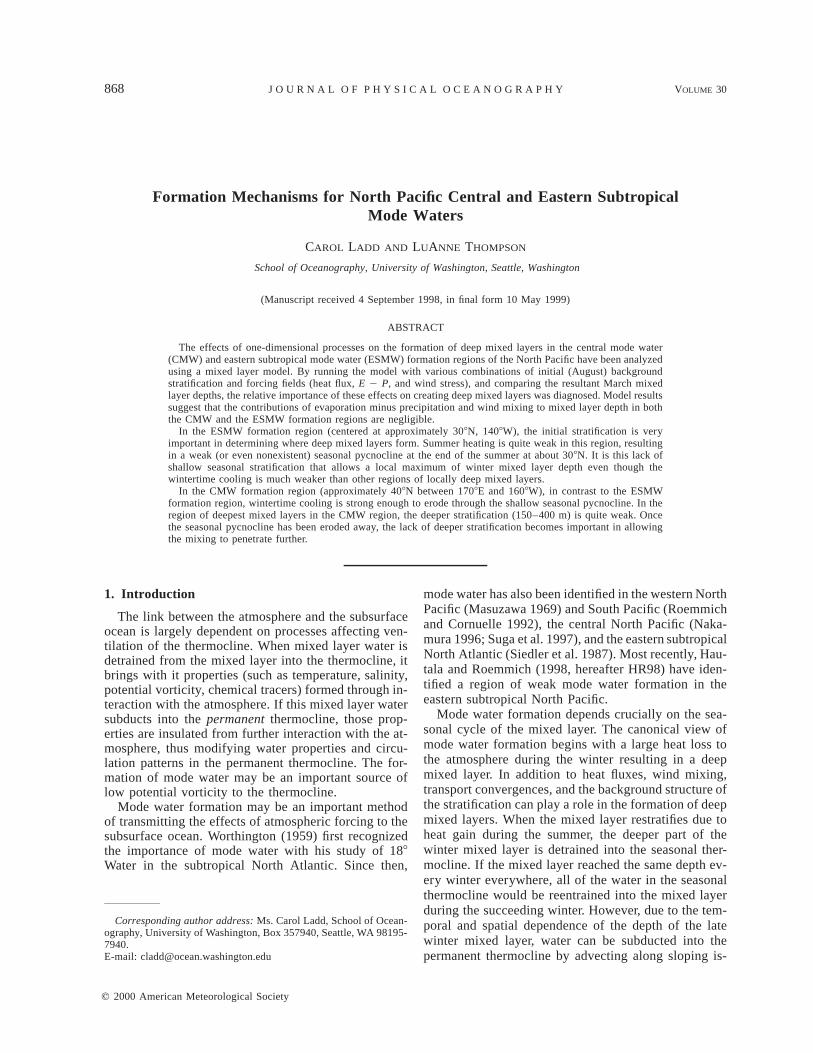
FIG. 2. Seasonal cycle (averaged along 28.58N, 149.58E–130.58W) of net heat flux from da Silva et al. (1994),mixed layer depth calculated from the World Ocean Atlas 1994, and mixed layer depth calculated by the model.

for each grid point (the results at each horizontal gridpoint do not effect the other grid points).

We have defined the MLD as the depth at which su

is 0.125 kg m23 different from the sea surface (followingQiu and Huang 1995). As the heat flux changes frompositive (into the ocean) to negative (out of the ocean)in the autumn, the mixed layer begins to deepen (Fig.2). The maximum heat flux out of the ocean averagedalong 28.58N occurs in December and does not becomepositive (into the ocean) until April. Averaged along28.58N, the MLD calculated by the model deepens morequickly than the MLD calculated from the WOA cli-matology resulting in a difference of roughly 90 m bythe end of the run (March).

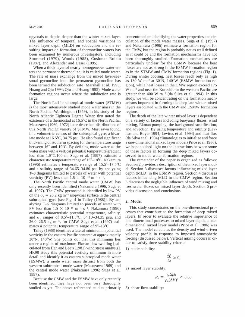
Both the March MLDs calculated from the WOA cli-matology (Fig. 3a) and those resulting from the controlrun (Fig. 3b) exhibit features thought to be associatedwith mode water formation regions. A maximum inMarch MLD (.220 m, Fig. 3a) south of the Kuroshio(308–358N, 1408–1558E) is associated with the westernsubtropical mode water (Masuzawa 1969). The STMWformation region is just outside of the model domain tothe west. A local maximum associated with the ESMWformation region is apparent in both the MLD calculatedfrom the WOA climatology (.120 m) and those cal-culated by the model (.160 m). This ESMW formationregion is centered at approximately 308N, 1408W in theeastern Pacific between Hawaii and the west coast ofNorth America. In addition, a broad band of deep mixedlayer (.240 m), associated with the central mode water(Nakamura 1996; Suga et al. 1997) is apparent in bothcalculations centered on approximately 408N extendingfrom about 1508E to the date line.

Although the spatial patterns are similar, the mag-nitudes are quite different, especially in the western Pa-cific. The model tends to overestimate MLDs and un-derestimate SST over most of the model domain relativeto the WOA climatology. This overestimation is prob-ably partially attributable to the effects of advection,especially in the western Pacific where the path of theKuroshio, bringing warm water north, would be ex-pected to have a large impact. An influx of warm surfacewater would tend to increase the stratification, whichwould decrease convective mixing.

In addition, due to the heavy spatial and temporal

smoothing in the WOA climatology, maxima in MLDcalculated from the climatology would tend to be un-derestimated. Spatial averaging tends to smooth out ex-tremes in gradients resulting in overestimates of minimaand underestimates of maxima. This results in an un-derestimate of MLD and an overestimate of stratificationin the weakly stratified part of the water column at depth.In fact, mixed layer depths calculated from WOCEP16N CTD data taken along 1528W in the North Pacificin March (McTaggart and Mangum 1995) show maxi-mum mixed layer depths reaching as deep as 140 m(around 308–358N), while those calculated from theWOA in the same region are less than 100 m. Thus,smoothing in the WOA and the resulting underestimateof MLDs may be partially responsible for the differencesbetween MLDs calculated from the WOA and thosecalculated by the model. However, the effects of ad-vection and other three-dimensional processes (neglect-ed by the model) are probably much more important inexplaining these differences.

An additional source of error comes from the fact thatheat fluxes are notoriously difficult to determine. Heatflux climatologies such as the ASMD can be expectedto have errors on the order of 20 W m22 (D. E. Harrison1998, personal communication). So some of the differ-ence between the model results and the WOA clima-tology may be due to errors in the heat flux forcing. Toanalyze the effects of possible errors in the heat fluxclimatology, we ran the model for two separate merid-ional sections with cooling reduced by 10 W m22.Throughout this work, we will be concentrating on twomeridional sections: 1) along 179.58E, slicing throughthe MLD maximum associated with the CMW, and 2)along 140.58W, associated with the ESMW. The differ-ences between the model March MLD and SST andthose calculated from the WOA average almost 46 mand 0.758C, averaged along 179.58E, with the modelmixed layer deeper and colder than the WOA mixedlayer. When the model is run with reduced cooling, thedifferences are reduced to about 24 m and 0.368C, abouthalf the original differences. Along 140.58W, the dif-ferences were smaller than along 179.58E: almost 33 min MLD and 0.638C in SST. The results of reducing thecooling reduced the difference in MLD to about 21 mand SST to 0.168C. Thus errors in the heat flux cli-


←

FIG. 3. March mixed layer depth (color ; in meters) and sea surface temperature (black contours; contour interval: 28C). Red contoursshow Mar outcrops of the su 5 26.25 and 25.0 kg m23 surfaces. Mixed layer depth is defined as the depth at which su is 0.125 kg m23

different from the sea surface. (a) Calculated from the World Ocean Atlas 1994. The black box illustrates the model domain. (b) Calculatedfrom the model.

matology could certainly be a substantial part of thedifference between modeled and observed MLD andSST.

The fact that the model gives deep mixed layers inthe right places (as compared to the WOA) is encour-aging. Since the model is initialized in late summerwhen the shallow stratification is the strongest, the one-dimensional processes, along with the initial stratifica-tion, included in the model must be at least partly re-sponsible for the locations of the maxima in MLD. Ourgoal is to quantify the relative importance of wind mix-ing, buoyancy fluxes, and stratification on creating deepmixed layers in certain regions. Because of the simpleone-dimensional nature of the model, it can be quiteuseful for analyzing the various effects of these pro-cesses and features on MLD, especially away from thewestern boundary where advection plays a very im-portant role.

3. Eastern subtropical mode water (140.58W)

Using XBT data, HR98 identify the eastern subtrop-ical mode water by a zone of minimum PV (defined interms of temperature: PV 5 f ]T/]z) in the vertical cen-tered at slightly more than 100-m depth. The PV min-imum (calculated here in terms of density: PV 5

f ]su/]z) is apparent in a zonal section of annually21r0

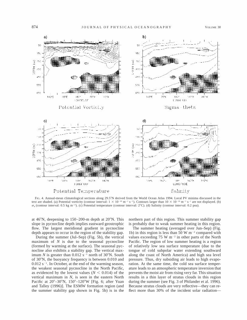
averaged WOA data at 29.58N [Fig. 4a: after Nakamura(1996)]. The ESMW appears as a bullet of PV less than3.0 3 10210 m21 s21 located at 1408W at about 100-mdepth. The associated su (25.0–25.5 kg m23) (Fig. 4b)and temperature (178–198C) (Fig. 4c) ranges of this localPV minimum are consistent with those calculated byHR98 (24.0–25.4 kg m23; 168–228C). The salinity rangeof the ESMW is approximately 34.4–35.0 psu (Fig. 4d).The ESMW PV minimum lies just to the west of asalinity front associated with a tongue of fresh subpolarwater extending southward along the coast of NorthAmerica. To the west of this front, salinity has a desta-bilizing effect on the water column (saltier water over-lying fresher water) while to the east of the front, salinitycontributes to the stability of the water column. Fartherto the east and deeper are stronger minima (PV , 2.03 10210 m21 s21) associated with the CMW (discussedin section 4) and STMW.

By superimposing contours of annual-mean acceler-ation potential on maps of PV on ESMW isopycnals,HR98 show that the mode water is circulated southwardin the eastern part of the subtropical gyre away fromthe wintertime outcrop (the presumed formation region).Over the course of the year, the PV minimum shifts

toward the southwest and weakens. The remains of thePV minimum water is found at 208–258N, 1558–1308Win early winter. (The PV minimum can be seen in theWOA data as far south as 248N.) The PV minimumshifts roughly 78–88 latitude in 8 months, giving a roughpropagation speed of 4 cm s21 (assuming purely merid-ional flow).

The formation region for ESMW is readily apparentby superimposing March SST contours and su outcropson a map of MLD (all derived from the WOA) (Fig.3a). In a region centered at approximately 308N, 1408Wa locally deep mixed layer (MLD . 120 m) coincideswith March surface temperatures between 168 and 208Cand lies just north of the su 5 25.0 kg m23 outcrop.

In the ESMW formation region (centered at 308N,1408W) winter cooling (Oct–Mar) averages only 90 Wm22 (da Silva et al. 1994). Because winter heat fluxesare small in the ESMW formation region (as comparedto the CMW and STMW formation regions), the causeof the deep mixed layer has been unclear. HR98 suggestthat the moderate winter heat loss observed in this re-gion could induce convective mixed layer deepening ifthe water column was preconditioned toward lower sta-bility.

Roden (1970, 1972) first identified a lateral minimumin the vertical stability in the North Pacific and termedit the ‘‘stability gap.’’ This region of reduced stabilityoccurs in the subarctic–subtropical transition zone.North of the transition zone, stability is dictated by astrong permanent halocline. In the subtropical waterssouth of the transition zone, a strong thermocline resultsin high stability. In the transition zone in between, sub-polar and subtropical water masses are both present,resulting in weaker stability. The reduced stability mayallow vertical mixing to penetrate much deeper andcould be one factor allowing the formation of modewaters in certain regions. Yuan and Talley (1996) cal-culate the horizontal minimum of vertical maximumbuoyancy frequency from the Levitus (1982) winterdata. They find that the stability gap occurs around 408Nin the western and central North Pacific. Another branchof the minimum is found near 308N, coinciding withthe ESMW formation region in the eastern Pacific.

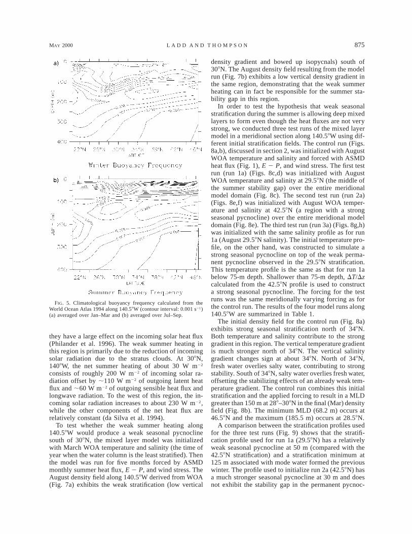
The buoyancy frequency (N) along 140.58W calcu-lated from WOA (Fig. 5) shows the stability gap quiteclearly. Averaged over the winter (Jan–Mar) (Fig. 5a),the maximum (in the vertical) buoyancy frequency isgreater than 0.009 s21 except between 288 and 318N—the stability gap—where N is between 0.008 and 0.009s21. This maximum is associated with the main pyc-nocline and is observed at depth approximately 125 m


FIG. 4. Annual-mean climatological sections along 29.58N derived from the World Ocean Atlas 1994. Local PV minima discussed in thetext are shaded. (a) Potential vorticity (contour interval: 1 3 10210 m21 s21). Contours larger than 10 3 10210 m21 s21 are not displayed. (b)su (contour interval: 0.5 kg m23). (c) Potential temperature (contour interval: 28C). (d) Salinity (contour interval: 0.2 psu).

at 468N, deepening to 150–200-m depth at 208N. Thisslope in pycnocline depth implies eastward geostrophicflow. The largest meridional gradient in pycnoclinedepth appears to occur in the region of the stability gap.

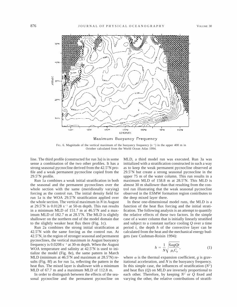
During the summer (Jul–Sep) (Fig. 5b), the verticalmaximum of N is due to the seasonal pycnocline(formed by warming at the surface). The seasonal pyc-nocline also exhibits a stability gap. The vertical max-imum N is greater than 0.012 s21 north of 308N. Southof 308N, the buoyancy frequency is between 0.010 and0.012 s21. In October, at the end of the warming season,the weakest seasonal pycnocline in the North Pacific,as evidenced by the lowest values (N , 0.014) of thevertical maximum in N, is seen in the eastern NorthPacific at 208–308N, 1508–1208W [Fig. 6; after Yuanand Talley (1996)]. The ESMW formation region (andthe summer stability gap shown in Fig. 5b) is in the

northern part of this region. This summer stability gapis probably due to weak summer heating in this region.

The summer heating (averaged over Jun–Sep) (Fig.1b) in this region is less than 50 W m22 compared withvalues exceeding 75 W m22 in other parts of the NorthPacific. The region of low summer heating is a regionof relatively low sea surface temperature (due to thetongue of cold subpolar water extending southwardalong the coast of North America) and high sea levelpressure. Thus, dry subsiding air leads to high evapo-ration. At the same time, the cold sea surface temper-ature leads to an atmospheric temperature inversion thatprevents the moist air from rising very far. This situationresults in a thin layer of stratus clouds in this regionduring the summer (see Fig. 3 of Philander et al. 1996).Because stratus clouds are very reflective—they can re-flect more than 30% of the incident solar radiation—


FIG. 5. Climatological buoyancy frequency calculated from theWorld Ocean Atlas 1994 along 140.58W (contour interval: 0.001 s21)(a) averaged over Jan–Mar and (b) averaged over Jul–Sep.

they have a large effect on the incoming solar heat flux(Philander et al. 1996). The weak summer heating inthis region is primarily due to the reduction of incomingsolar radiation due to the stratus clouds. At 308N,1408W, the net summer heating of about 30 W m22

consists of roughly 200 W m22 of incoming solar ra-diation offset by ;110 W m22 of outgoing latent heatflux and ;60 W m22 of outgoing sensible heat flux andlongwave radiation. To the west of this region, the in-coming solar radiation increases to about 230 W m22,while the other components of the net heat flux arerelatively constant (da Silva et al. 1994).

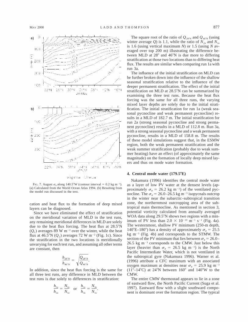
To test whether the weak summer heating along140.58W would produce a weak seasonal pycnoclinesouth of 308N, the mixed layer model was initializedwith March WOA temperature and salinity (the time ofyear when the water column is the least stratified). Thenthe model was run for five months forced by ASMDmonthly summer heat flux, E 2 P, and wind stress. TheAugust density field along 140.58W derived from WOA(Fig. 7a) exhibits the weak stratification (low vertical

density gradient and bowed up isopycnals) south of308N. The August density field resulting from the modelrun (Fig. 7b) exhibits a low vertical density gradient inthe same region, demonstrating that the weak summerheating can in fact be responsible for the summer sta-bility gap in this region.

In order to test the hypothesis that weak seasonalstratification during the summer is allowing deep mixedlayers to form even though the heat fluxes are not verystrong, we conducted three test runs of the mixed layermodel in a meridional section along 140.58W using dif-ferent initial stratification fields. The control run (Figs.8a,b), discussed in section 2, was initialized with AugustWOA temperature and salinity and forced with ASMDheat flux (Fig. 1), E 2 P, and wind stress. The first testrun (run 1a) (Figs. 8c,d) was initialized with AugustWOA temperature and salinity at 29.58N (the middle ofthe summer stability gap) over the entire meridionalmodel domain (Fig. 8c). The second test run (run 2a)(Figs. 8e,f) was initialized with August WOA temper-ature and salinity at 42.58N (a region with a strongseasonal pycnocline) over the entire meridional modeldomain (Fig. 8e). The third test run (run 3a) (Figs. 8g,h)was initialized with the same salinity profile as for run1a (August 29.58N salinity). The initial temperature pro-file, on the other hand, was constructed to simulate astrong seasonal pycnocline on top of the weak perma-nent pycnocline observed in the 29.58N stratification.This temperature profile is the same as that for run 1abelow 75-m depth. Shallower than 75-m depth, DT/Dzcalculated from the 42.58N profile is used to constructa strong seasonal pycnocline. The forcing for the testruns was the same meridionally varying forcing as forthe control run. The results of the four model runs along140.58W are summarized in Table 1.

The initial density field for the control run (Fig. 8a)exhibits strong seasonal stratification north of 348N.Both temperature and salinity contribute to the stronggradient in this region. The vertical temperature gradientis much stronger north of 348N. The vertical salinitygradient changes sign at about 348N. North of 348N,fresh water overlies salty water, contributing to strongstability. South of 348N, salty water overlies fresh water,offsetting the stabilizing effects of an already weak tem-perature gradient. The control run combines this initialstratification and the applied forcing to result in a MLDgreater than 150 m at 288–308N in the final (Mar) densityfield (Fig. 8b). The minimum MLD (68.2 m) occurs at46.58N and the maximum (185.5 m) occurs at 28.58N.

A comparison between the stratification profiles usedfor the three test runs (Fig. 9) shows that the stratifi-cation profile used for run 1a (29.58N) has a relativelyweak seasonal pycnocline at 50 m (compared with the42.58N stratification) and a stratification minimum at125 m associated with mode water formed the previouswinter. The profile used to initialize run 2a (42.58N) hasa much stronger seasonal pycnocline at 30 m and doesnot exhibit the stability gap in the permanent pycnoc-


FIG. 6. Magnitude of the vertical maximum of the buoyancy frequency (s21) in the upper 400 m inOctober calculated from the World Ocean Atlas 1994.

line. The third profile (constructed for run 3a) is in somesense a combination of the two other profiles. It has astrong seasonal pycnocline derived from the 42.58N pro-file and a weak permanent pycnocline copied from the29.58N profile.

Run 1a combines a weak initial stratification in boththe seasonal and the permanent pycnoclines over thewhole section with the same (meridionally varying)forcing as the control run. The initial density field forrun 1a is the WOA 29.58N stratification applied overthe whole section. The vertical maximum in N in Augustat 29.58N is 0.0128 s21 at 50-m depth. This run resultsin a minimum MLD of 151.7 m at 46.58N and a max-imum MLD of 182.7 m at 28.58N. The MLD is slightlyshallower on the northern end of the model domain dueto the slightly weaker heat flux there (Fig. 1c).

Run 2a combines the strong initial stratification at42.58N with the same forcing as the control run. At42.58N, in the region of stronger seasonal and permanentpycnoclines, the vertical maximum in August buoyancyfrequency is 0.0208 s21 at 30-m depth. When the AugustWOA temperature and salinity at 42.58N is used to ini-tialize the model (Fig. 8e), the same pattern in MarchMLD (minimum at 46.58N and maximum at 28.58N) re-sults (Fig. 8f) as for run 1a, reflecting the pattern in theheat flux. The mixed layer is shallower with a minimumMLD of 67.7 m and a maximum MLD of 112.8 m.

In order to distinguish between the effects of the sea-sonal pycnocline and the permanent pycnocline on

MLD, a third model run was executed. Run 3a wasinitialized with a stratification constructed in such a wayas to keep the weak permanent pycnocline observed at29.58N but create a strong seasonal pycnocline in theupper 75 m of the water column. This run results in amaximum MLD of 158.8 m at 28.58N. This MLD isalmost 30 m shallower than that resulting from the con-trol run illustrating that the weak seasonal pycnoclineobserved in the ESMW formation region contributes tothe deep mixed layer there.

In these one-dimensional model runs, the MLD is afunction of the heat flux forcing and the initial strati-fication. The following analysis is an attempt to quantifythe relative effects of these two factors. In the simplecase of a water column that is initially linearly stratifiedand subject to a constant surface cooling Q over a timeperiod t, the depth h of the convective layer can becalculated from the heat and the mechanical energy bud-gets (see Cushman-Roisin 1994):

1 6agQth 5 , (1)!N r C0 p

where a is the thermal expansion coefficient, g is grav-itational acceleration, and N is the buoyancy frequency.In this simple case, the influences of stratification (N 2)and heat flux (Q) on MLD are inversely proportional toeach other. Therefore, by keeping N 2 or Q fixed andvarying the other, the relative contributions of stratifi-


FIG. 7. August su along 140.58W (contour interval 5 0.2 kg m23).(a) Calculated from the World Ocean Atlas 1994. (b) Resulting fromthe model run discussed in the text.

cation and heat flux to the formation of deep mixedlayers can be diagnosed.

Since we have eliminated the effect of stratificationon the meridional variation of MLD in the test runs,any remaining meridional differences in MLD are solelydue to the heat flux forcing. The heat flux at 28.58N(Q1) averages 89 W m22 over the winter, while the heatflux at 46.58N (Q2) averages 72 W m22 (Fig. 1c). Sincethe stratification in the two locations is meridionallyunvarying for each test run, and assuming all other termsare constant, then

h Q288N 288N5 .!h Q468N 468N

In addition, since the heat flux forcing is the same forall three test runs, any difference in MLD between thetest runs is due solely to differences in stratification:

h N h N1a 2a 1a 3a5 or 5 .h N h N2a 1a 3a 1a

The square root of the ratio of Q288N and Q468N (usingwinter average Q) is 1.1, while the ratio of N2a and N1a

is 1.6 (using vertical maximum N) or 1.5 (using N av-eraged over top 200 m) illustrating the difference be-tween MLD at 288 and 468N is due more to differingstratification at those two locations than to differing heatflux. The results are similar when comparing run 1a withrun 3a.

The influence of the initial stratification on MLD canbe further broken down into the influence of the shallowseasonal stratification relative to the influence of thedeeper permanent stratification. The effect of the initialstratification on MLD at 28.58N can be summarized byexamining the three test runs. Because the heat fluxforcing was the same for all three runs, the varyingmixed layer depths are solely due to the initial strati-fication. The initial stratification for run 1a (weak sea-sonal pycnocline and weak permanent pycnocline) re-sults in a MLD of 182.7 m. The initial stratification forrun 2a (strong seasonal pycnocline and strong perma-nent pycnocline) results in a MLD of 112.8 m. Run 3a,with a strong seasonal pycnocline and a weak permanentpycnocline, results in a MLD of 158.8 m. The resultsof these model simulations suggest that, in the ESMWregion, both the weak permanent stratification and theweak summer stratification (probably due to weak sum-mer heating) have an effect (of approximately the samemagnitude) on the formation of locally deep mixed lay-ers and thus on mode water formation.

4. Central mode water (179.58E)

Nakamura (1996) identifies the central mode wateras a layer of low PV water at the densest levels (ap-proximately su 5 26.2 kg m23) of the ventilated pyc-nocline. The su 5 26.0–26.5 kg m23 isopycnals outcropin the winter near the subarctic–subtropical transitionzone, the northernmost outcropping area of the sub-tropical main thermocline. As mentioned in section 3,potential vorticity calculated from annually averagedWOA data along 29.58N shows two regions with a min-imum of PV less than 2.0 3 10210 m21 s21 (Fig. 4a).The westernmost, shallow PV minimum (250-m depth,1408E–1808) has a density of approximately su 5 25.5kg m23 (Fig. 4b) and corresponds to the STMW. Thesection of the PV minimum that lies between su 5 26.0–26.5 kg m23 corresponds to the CMW. Just below thislayer (heavier than su 5 26.5 kg m23) is the NorthPacific Intermediate Water, which is not ventilated inthe subtropical gyre (Nakamura 1996). Warner et al.(1996) attribute a CFC maximum with an associatedoxygen maximum at densities near su 5 25.9 kg m23

(118–148C) at 248N between 1608 and 1408W to theCMW.

The entire CMW thermostad appears to lie in a zoneof eastward flow, the North Pacific Current (Suga et al.1997). Eastward flow with a slight southward compo-nent is dominant over the formation region. The typical


←

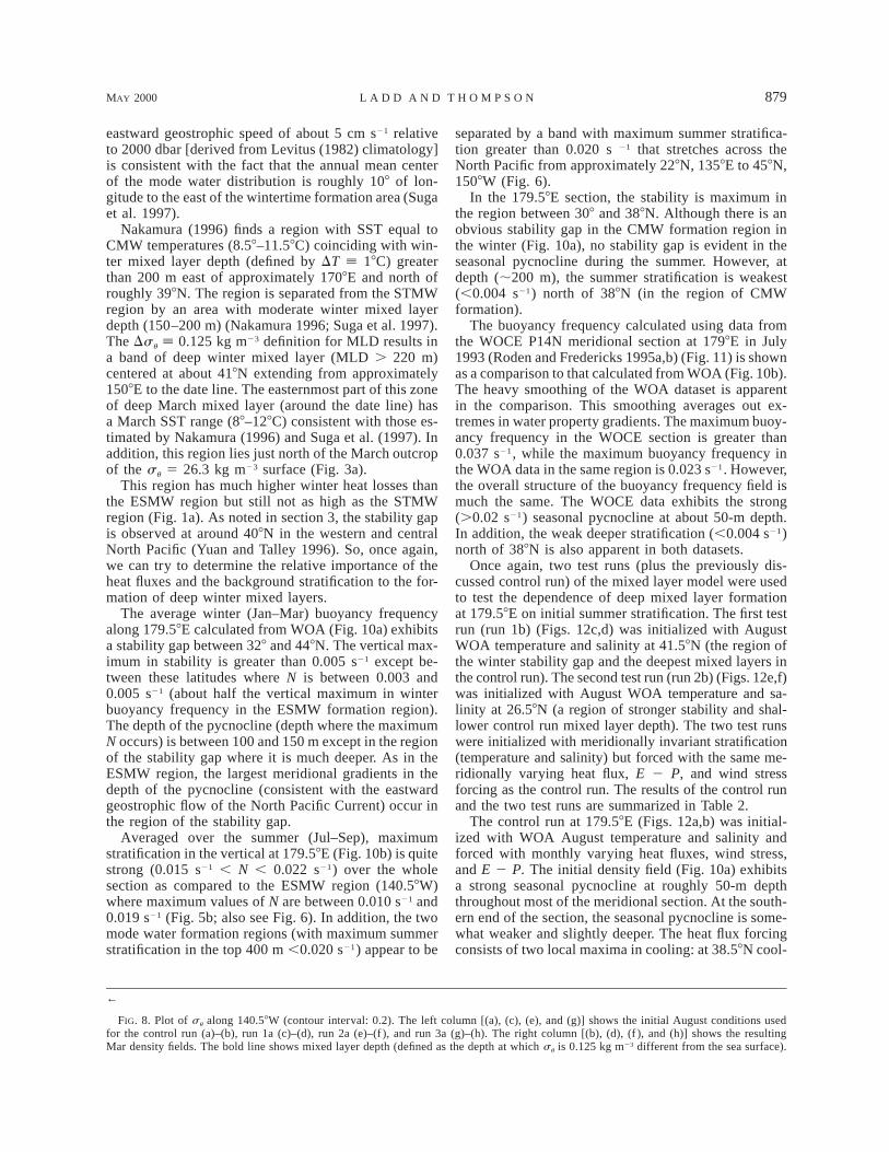
FIG. 8. Plot of su along 140.58W (contour interval: 0.2). The left column [(a), (c), (e), and (g)] shows the initial August conditions usedfor the control run (a)–(b), run 1a (c)–(d), run 2a (e)–(f ), and run 3a (g)–(h). The right column [(b), (d), (f ), and (h)] shows the resultingMar density fields. The bold line shows mixed layer depth (defined as the depth at which su is 0.125 kg m23 different from the sea surface).

eastward geostrophic speed of about 5 cm s21 relativeto 2000 dbar [derived from Levitus (1982) climatology]is consistent with the fact that the annual mean centerof the mode water distribution is roughly 108 of lon-gitude to the east of the wintertime formation area (Sugaet al. 1997).

Nakamura (1996) finds a region with SST equal toCMW temperatures (8.58–11.58C) coinciding with win-ter mixed layer depth (defined by DT [ 18C) greaterthan 200 m east of approximately 1708E and north ofroughly 398N. The region is separated from the STMWregion by an area with moderate winter mixed layerdepth (150–200 m) (Nakamura 1996; Suga et al. 1997).The Dsu [ 0.125 kg m23 definition for MLD results ina band of deep winter mixed layer (MLD . 220 m)centered at about 418N extending from approximately1508E to the date line. The easternmost part of this zoneof deep March mixed layer (around the date line) hasa March SST range (88–128C) consistent with those es-timated by Nakamura (1996) and Suga et al. (1997). Inaddition, this region lies just north of the March outcropof the su 5 26.3 kg m23 surface (Fig. 3a).

This region has much higher winter heat losses thanthe ESMW region but still not as high as the STMWregion (Fig. 1a). As noted in section 3, the stability gapis observed at around 408N in the western and centralNorth Pacific (Yuan and Talley 1996). So, once again,we can try to determine the relative importance of theheat fluxes and the background stratification to the for-mation of deep winter mixed layers.

The average winter (Jan–Mar) buoyancy frequencyalong 179.58E calculated from WOA (Fig. 10a) exhibitsa stability gap between 328 and 448N. The vertical max-imum in stability is greater than 0.005 s21 except be-tween these latitudes where N is between 0.003 and0.005 s21 (about half the vertical maximum in winterbuoyancy frequency in the ESMW formation region).The depth of the pycnocline (depth where the maximumN occurs) is between 100 and 150 m except in the regionof the stability gap where it is much deeper. As in theESMW region, the largest meridional gradients in thedepth of the pycnocline (consistent with the eastwardgeostrophic flow of the North Pacific Current) occur inthe region of the stability gap.

Averaged over the summer (Jul–Sep), maximumstratification in the vertical at 179.58E (Fig. 10b) is quitestrong (0.015 s21 , N , 0.022 s21) over the wholesection as compared to the ESMW region (140.58W)where maximum values of N are between 0.010 s21 and0.019 s21 (Fig. 5b; also see Fig. 6). In addition, the twomode water formation regions (with maximum summerstratification in the top 400 m ,0.020 s21) appear to be

separated by a band with maximum summer stratifica-tion greater than 0.020 s 21 that stretches across theNorth Pacific from approximately 228N, 1358E to 458N,1508W (Fig. 6).

In the 179.58E section, the stability is maximum inthe region between 308 and 388N. Although there is anobvious stability gap in the CMW formation region inthe winter (Fig. 10a), no stability gap is evident in theseasonal pycnocline during the summer. However, atdepth (;200 m), the summer stratification is weakest(,0.004 s21) north of 388N (in the region of CMWformation).

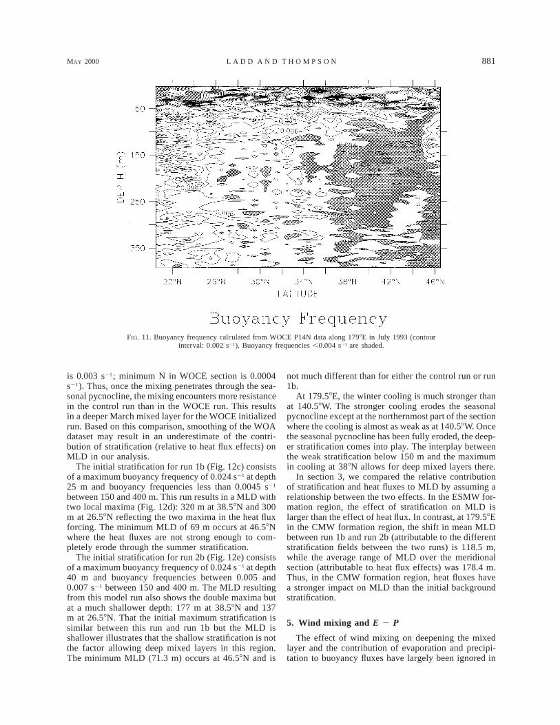
The buoyancy frequency calculated using data fromthe WOCE P14N meridional section at 1798E in July1993 (Roden and Fredericks 1995a,b) (Fig. 11) is shownas a comparison to that calculated from WOA (Fig. 10b).The heavy smoothing of the WOA dataset is apparentin the comparison. This smoothing averages out ex-tremes in water property gradients. The maximum buoy-ancy frequency in the WOCE section is greater than0.037 s21, while the maximum buoyancy frequency inthe WOA data in the same region is 0.023 s21. However,the overall structure of the buoyancy frequency field ismuch the same. The WOCE data exhibits the strong(.0.02 s21) seasonal pycnocline at about 50-m depth.In addition, the weak deeper stratification (,0.004 s21)north of 388N is also apparent in both datasets.

Once again, two test runs (plus the previously dis-cussed control run) of the mixed layer model were usedto test the dependence of deep mixed layer formationat 179.58E on initial summer stratification. The first testrun (run 1b) (Figs. 12c,d) was initialized with AugustWOA temperature and salinity at 41.58N (the region ofthe winter stability gap and the deepest mixed layers inthe control run). The second test run (run 2b) (Figs. 12e,f)was initialized with August WOA temperature and sa-linity at 26.58N (a region of stronger stability and shal-lower control run mixed layer depth). The two test runswere initialized with meridionally invariant stratification(temperature and salinity) but forced with the same me-ridionally varying heat flux, E 2 P, and wind stressforcing as the control run. The results of the control runand the two test runs are summarized in Table 2.

The control run at 179.58E (Figs. 12a,b) was initial-ized with WOA August temperature and salinity andforced with monthly varying heat fluxes, wind stress,and E 2 P. The initial density field (Fig. 10a) exhibitsa strong seasonal pycnocline at roughly 50-m depththroughout most of the meridional section. At the south-ern end of the section, the seasonal pycnocline is some-what weaker and slightly deeper. The heat flux forcingconsists of two local maxima in cooling: at 38.58N cool-


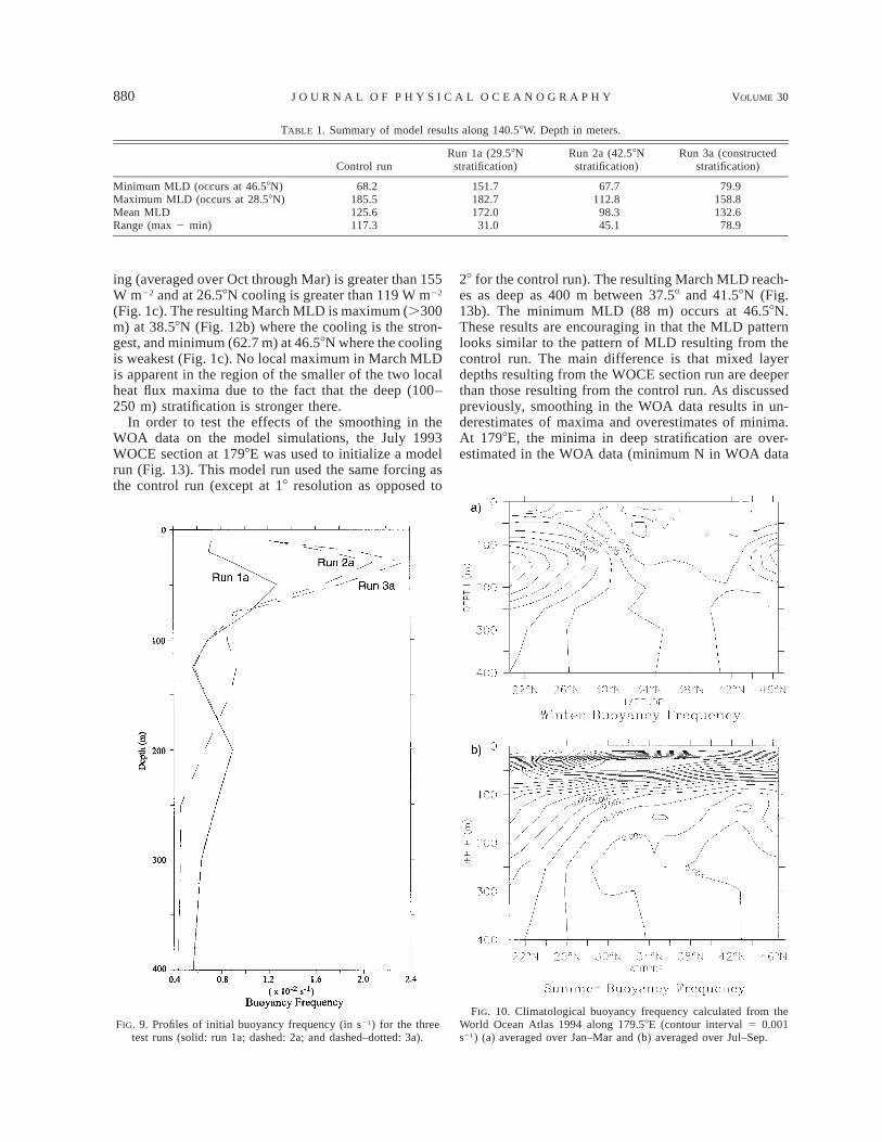
TABLE 1. Summary of model results along 140.58W. Depth in meters.

Control runRun 1a (29.58N

stratification)Run 2a (42.58N

stratification)Run 3a (constructed

stratification)

Minimum MLD (occurs at 46.58N) 68.2 151.7 67.7 79.9Maximum MLD (occurs at 28.58N) 185.5 182.7 112.8 158.8Mean MLD 125.6 172.0 98.3 132.6Range (max 2 min) 117.3 31.0 45.1 78.9

FIG. 10. Climatological buoyancy frequency calculated from theWorld Ocean Atlas 1994 along 179.58E (contour interval 5 0.001s21) (a) averaged over Jan–Mar and (b) averaged over Jul–Sep.

FIG. 9. Profiles of initial buoyancy frequency (in s21) for the threetest runs (solid: run 1a; dashed: 2a; and dashed–dotted: 3a).

ing (averaged over Oct through Mar) is greater than 155W m22 and at 26.58N cooling is greater than 119 W m22

(Fig. 1c). The resulting March MLD is maximum (.300m) at 38.58N (Fig. 12b) where the cooling is the stron-gest, and minimum (62.7 m) at 46.58N where the coolingis weakest (Fig. 1c). No local maximum in March MLDis apparent in the region of the smaller of the two localheat flux maxima due to the fact that the deep (100–250 m) stratification is stronger there.

In order to test the effects of the smoothing in theWOA data on the model simulations, the July 1993WOCE section at 1798E was used to initialize a modelrun (Fig. 13). This model run used the same forcing asthe control run (except at 18 resolution as opposed to

28 for the control run). The resulting March MLD reach-es as deep as 400 m between 37.58 and 41.58N (Fig.13b). The minimum MLD (88 m) occurs at 46.58N.These results are encouraging in that the MLD patternlooks similar to the pattern of MLD resulting from thecontrol run. The main difference is that mixed layerdepths resulting from the WOCE section run are deeperthan those resulting from the control run. As discussedpreviously, smoothing in the WOA data results in un-derestimates of maxima and overestimates of minima.At 1798E, the minima in deep stratification are over-estimated in the WOA data (minimum N in WOA data


FIG. 11. Buoyancy frequency calculated from WOCE P14N data along 1798E in July 1993 (contourinterval: 0.002 s21). Buoyancy frequencies ,0.004 s21 are shaded.

is 0.003 s21; minimum N in WOCE section is 0.0004s21). Thus, once the mixing penetrates through the sea-sonal pycnocline, the mixing encounters more resistancein the control run than in the WOCE run. This resultsin a deeper March mixed layer for the WOCE initializedrun. Based on this comparison, smoothing of the WOAdataset may result in an underestimate of the contri-bution of stratification (relative to heat flux effects) onMLD in our analysis.

The initial stratification for run 1b (Fig. 12c) consistsof a maximum buoyancy frequency of 0.024 s21 at depth25 m and buoyancy frequencies less than 0.0045 s21

between 150 and 400 m. This run results in a MLD withtwo local maxima (Fig. 12d): 320 m at 38.58N and 300m at 26.58N reflecting the two maxima in the heat fluxforcing. The minimum MLD of 69 m occurs at 46.58Nwhere the heat fluxes are not strong enough to com-pletely erode through the summer stratification.

The initial stratification for run 2b (Fig. 12e) consistsof a maximum buoyancy frequency of 0.024 s21 at depth40 m and buoyancy frequencies between 0.005 and0.007 s21 between 150 and 400 m. The MLD resultingfrom this model run also shows the double maxima butat a much shallower depth: 177 m at 38.58N and 137m at 26.58N. That the initial maximum stratification issimilar between this run and run 1b but the MLD isshallower illustrates that the shallow stratification is notthe factor allowing deep mixed layers in this region.The minimum MLD (71.3 m) occurs at 46.58N and is

not much different than for either the control run or run1b.

At 179.58E, the winter cooling is much stronger thanat 140.58W. The stronger cooling erodes the seasonalpycnocline except at the northernmost part of the sectionwhere the cooling is almost as weak as at 140.58W. Oncethe seasonal pycnocline has been fully eroded, the deep-er stratification comes into play. The interplay betweenthe weak stratification below 150 m and the maximumin cooling at 388N allows for deep mixed layers there.

In section 3, we compared the relative contributionof stratification and heat fluxes to MLD by assuming arelationship between the two effects. In the ESMW for-mation region, the effect of stratification on MLD islarger than the effect of heat flux. In contrast, at 179.58Ein the CMW formation region, the shift in mean MLDbetween run 1b and run 2b (attributable to the differentstratification fields between the two runs) is 118.5 m,while the average range of MLD over the meridionalsection (attributable to heat flux effects) was 178.4 m.Thus, in the CMW formation region, heat fluxes havea stronger impact on MLD than the initial backgroundstratification.

5. Wind mixing and E 2 P

The effect of wind mixing on deepening the mixedlayer and the contribution of evaporation and precipi-tation to buoyancy fluxes have largely been ignored in


TABLE 2. Summary of model results along 179.58E. Depth inmeters.

Controlrun

Run 1b (41.58Nstratification)

Run 2b (26.58Nstratification)

Minimum MLD(occurs at 46.58N)

62.7 69.0 71.3

Maximum MLD(occurs at 38.58N)

303.0 319.9 177.2

Mean MLD 164.2 247.7 129.2Range (max 2 min) 240.3 250.9 105.9

←

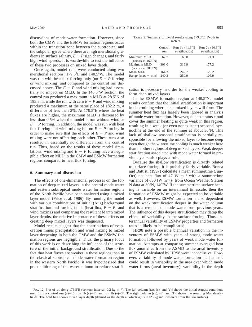
FIG. 12. Plot of su along 179.58E (contour interval: 0.2 kg m23). The left column [(a), (c), and (e)] shows the initial August conditionsused for the control run (a)–(b), run 1b (c)–(d), and run 2b (e)–(f ). The right column [(b), (d), and (f )] shows the resulting Mar densityfields. The bold line shows mixed layer depth (defined as the depth at which su is 0.125 kg m23 different from the sea surface).

discussions of mode water formation. However, sinceboth the CMW and the ESMW formation regions occurwithin the transition zone between the subtropical andthe subpolar gyres where there are high meridional gra-dients in surface salinity, E 2 P sign changes, and fairlyhigh wind speeds, it is worthwhile to test the influenceof these two processes on mixed layer depth.

Once again, model runs were conducted along twomeridional sections: 179.58E and 140.58W. The modelwas run with heat flux forcing only (no E 2 P forcingor wind mixing) and compared to the control run dis-cussed above. The E 2 P and wind mixing had essen-tially no impact on MLD. In the 140.58W section, thecontrol run produced a maximum in MLD at 28.58N of185.5 m, while the run with zero E 2 P and wind mixingproduced a maximum at the same place of 182.2 m, adifference of less than 2%. At 179.58E where the heatfluxes are higher, the maximum MLD is decreased byless than 0.5% when the model is run without wind orE 2 P forcing. In addition, the model was run with heatflux forcing and wind mixing but no E 2 P forcing inorder to make sure that the effects of E 2 P and windmixing were not offsetting each other. These runs alsoresulted in essentially no difference from the controlrun. Thus, based on the results of these model simu-lations, wind mixing and E 2 P forcing have a negli-gible effect on MLD in the CMW and ESMW formationregions compared to heat flux forcing.

6. Summary and discussion

The effects of one-dimensional processes on the for-mation of deep mixed layers in the central mode waterand eastern subtropical mode water formation regionsof the North Pacific have been analyzed using a mixedlayer model (Price et al. 1986). By running the modelwith various combinations of initial (Aug) backgroundstratification and forcing fields (heat flux, E 2 P, andwind mixing) and comparing the resultant March mixedlayer depths, the relative importance of these effects oncreating deep mixed layers was diagnosed.

Model results suggest that the contributions of evap-oration minus precipitation and wind mixing to mixedlayer deepening in both the CMW and the ESMW for-mation regions are negligible. Thus, the primary focusof this work is on describing the influence of the struc-ture of the initial background stratification. Due to thefact that heat fluxes are weaker in these regions than inthe classical subtropical mode water formation regionin the western North Pacific, it was hypothesized thatpreconditioning of the water column to reduce stratifi-

cation is necessary in order for the weaker cooling toform deep mixed layers.

In the ESMW formation region at 140.58N, modelresults confirm that the initial stratification is importantin determining where deep mixed layers will form. Thesummer heat flux has largely been ignored in analysisof mode water formation. However, due to stratus cloudcover the summer heating is quite weak in this region,resulting in a weak (or even nonexistent) seasonal pyc-nocline at the end of the summer at about 308N. Thislack of shallow seasonal stratification is partially re-sponsible for allowing the mixed layer to become deepeven though the wintertime cooling is much weaker herethan in other regions of deep mixed layers. Weak deeperstratification associated with mode water formed in pre-vious years also plays a role.

Because the shallow stratification is directly relatedto surface forcing, it is probably fairly variable. Roncaand Battisti (1997) calculate a mean summertime (Jun–Oct) net heat flux of 47 W m22 with a summertimevariance of 650 (W m22)2 from Ocean Weather StationN data at 308N, 1408W. If the summertime surface heat-ing is variable on an interannual timescale, then theformation of ESMW might be expected to be variableas well. However, ESMW formation is also dependenton the weak stratification deeper in the water columnthat is a remnant of mode water from previous years.The influence of this deeper stratification may damp theeffects of variability in the surface forcing. Thus, in-terannual variability of ESMW properties and formationrates is likely to be complicated.

HR98 note a possible biannual variation in the in-ventory of ESMW with years of strong mode waterformation followed by years of weak mode water for-mation. Attempts at comparing summer averaged heatflux anomalies from the ASMD to the areal inventoryof ESMW calculated by HR98 were inconclusive. How-ever, variability of mode water formation mechanismscould result in variability in the area over which modewater forms (areal inventory), variability in the depth


FIG. 13. Plot of su along 1798E (contour interval: 0.2 kg m23) (a) from WOCE P14N data in Jul 1993 and (b) resulting Mar density fieldfrom model run that was initialized with WOCE P14N data. The bold line shows mixed layer depth (defined as the depth at which su is0.125 kg m23 different from the sea surface).

to which it forms (magnitude of the PV minimum), var-iability in the temperature of mode water formed, ormore likely a combination of the three. It would prob-ably be more appropriate to compare the strength ofheat flux anomalies with the strength of the PV mini-mum.

Mixing between currently forming mode water andmode water formed in previous years may effect modewater properties. Namias and Born (1970, 1974) firstnoted a tendency for midlatitude SST anomalies to recurin succeeding winters without persisting through theintervening summer. They speculated that temperatureanomalies in the deep winter mixed layer could remainintact in the seasonal thermocline during the summer,insulated from surface processes by the shallow summerstratification. These anomalies could then affect the tem-perature of the succeeding winter’s deep mixed layer.In fact, Alexander and Deser (1995), using a one-di-mensional mixed layer model similar to the one usedin this study, find that vertical mixing processes allowocean temperature anomalies created over a deep wintermixed layer to be preserved below the surface in sum-mer to reappear in the mixed layer in the followingautumn. Using a three-dimensional model of the NorthPacific, Miller et al. (1994) find that this reemergencemechanism is weak over most of the central Pacific (inthe region of the California Current and the KuroshioExtension) but does occur in the vicinity of the ESMWformation region.

In the CMW formation region, in contrast to theESMW formation region, wintertime cooling is strongenough to erode through the shallow seasonal pycnoc-line. In the region of deepest mixed layers in the CMW

region, the deeper stratification (150–400 m) is quiteweak. Once the seasonal pycnocline has been fully erod-ed, the deeper stratification becomes important in al-lowing the mixing to penetrate further.

Of course this analysis, using the one-dimensionalmixed layer model, has ignored any advective effects.These effects are likely to be quite important in somelocations. In fact, a local maximum in WOA Marchmixed layer depth (Fig. 3a) of over 290 m occurs around1608E, approximately 198 to the west of the maximumMLD we have associated with the CMW formation re-gion. Suga et al. (1997) estimate an eastward geostroph-ic speed of approximately 5 cm s21 (;198 long. yr21)relative to 2000 dbar over this region. If the weak sub-surface stratification formed by the deep March mixedlayer at 1608E advected approximately 198 of longitudein a year, it could be responsible for the weak deepstratification that contributes to the formation of CMW.Attempts to follow up on this hypothesis by analyzingWOA data were unsuccessful. Some factors that maybe responsible for our lack of success in tracking theadvection of subsurface stratification include effects ofthe meridional component of currents or of verticalshear in the water column, which were not taken intoaccount in the analysis. In addition, the effects of tem-poral and spatial smoothing on the WOA data may havehad some influence.

The influence of horizontal advection on ESMW for-mation is not likely to be as important as to the CMWformation for a couple of reasons: 1) the shallow sea-sonal stratification is important to ESMW formation andthis weak stratification is more recently and locallyformed than the deeper stratification important to CMW


formation and 2) the ESMW formation region is in thebroad region of weaker southward flowing currents.

In addition to horizontal advection, Ekman pumpingmay also be important to deep mixed layer formation.In fact, Talley (1988) notes that the lateral minimum inpotential vorticity associated with the ESMW lies undera region of maximum Ekman downwelling [calculatedfrom Han and Lee’s (1981) wind stress analysis]. Onthe other hand, Nakamura (1996) points out that theCMW formation region lies in the subtropical gyre southof the zero Sverdrup function but in the upwelling re-gion north of the zero in Ekman pumping. He concludesthat Ekman pumping cannot be important in the sub-duction of CMW.

These conclusions are supported by Huang and Qiu(1994). They calculate subduction rates from Levitus(1982) climatology and Hellerman and Rosenstein(1983) wind stress data. Their calculations show a localmaximum in subduction rate greater than 25 m yr21

around 428N, 1608E that may be associated with CMWformation. This maximum is almost completely due tolateral induction (where water parcels move laterallyacross the sloping base of the mixed layer). In addition,a double maximum in subduction rate greater than 50m yr21 that may be associated with the ESMW is evidentin the region 208–308N, 1408–1208W. This maximum isdue to both lateral induction and vertical pumping inapproximately equal parts.

Formation of mode waters is obviously a complicatedprocess depending on the interplay of various oceanicand atmospheric factors. We have only focused on theone-dimensional processes that lead to deep mixed lay-ers, an important feature in mode water formation. Theformation and circulation of mode water is much morecomplex than this analysis would suggest.

Yasuda and Hanawa (1997) study decadal changes inthe STMW and the CMW by averaging together (sea-sonally) all data from the decade 1966–75 and com-paring it to data averaged over 1976–85. In the mid-1970s, a well-documented transition occurred in theNorth Pacific (Douglas et al. 1982; Nitta and Yamada1989; Graham 1994; Deser et al. 1996). This transitionresulted in a decrease in SST in the central North Pacificthat lasted into the 1980s. The transition has been shownto have a connection with variations in atmospheric cir-culation characterized by the Pacific–North American(PNA) pattern (Trenberth 1990; Wallace et al. 1990;Trenberth and Hurrel 1994). Yasuda and Hanawa (1997)find that the CMW was colder and more widely dis-tributed during 1976–85 compared to the previous de-cade. They attribute this cooling to increased Ekmanheat divergence in the CMW formation region causedby intensification of the westerlies (associated with anenhanced Aleutian low).

Zhang and Levitus (1997) provide observational ev-idence of decadal variability in the thermal structure ofthe subsurface ocean. They present evidence that thetemperature anomaly patterns rotate anticyclonically

around the subtropical gyre with a characteristic time-scale of approximately 20 yr. Maxima in the spatialpattern of this variability shows good correspondencewith the formation regions of the CMW and the ESMW,suggesting that variability in mode water formation inthese two regions may be related to decadal variabilityin the North Pacific.

Recent studies have suggested that water parcels sub-ducted in the subtropical North Pacific may provide alink between the midlatitude and the tropical ocean. Thislink may influence subtropical and tropical variabilityon decadal timescales (Gu and Philander 1997; Zhanget al. 1998). It has been hypothesized that subductedthermal anomalies can propagate equatorward in thethermocline (Gu and Philander 1996; Schneider et al.1999), eventually upwelling and affecting sea surfacetemperatures in the Tropics and perhaps the frequencyor magnitude of El Nino events. The atmosphere couldthen respond to the anomalous SST and, through tele-connections (Bjerknes 1966; Alexander 1992; Philander1990), affect the surface ocean in the subtropics thusinfluencing decadal variability. In fact, Schneider et al.(1999), using a dataset of BT, XBT, and CTD stationscompiled by White (1995), succeed in tracking anom-alies in the depth of the 128–188C isothermal layer fromthe central North Pacific to approximately 208N.

Because the western subtropical mode water isformed in, and primarily confined to, the recirculationregion of the western subtropical gyre, it is not likelyto be a participant in the subtropical–tropical exchange.General circulation models have been used to deducethe pathways taken by subducted water parcels (Gu andPhilander 1997). Results suggest that the water massesformed farther to the east, such as the ESMW, are themost likely to have an influence on the Tropics. Thus,an understanding of the circulation and variability ofthese mode waters is important to our understanding ofdecadal variability.

Acknowledgments. We are grateful to Susan Hautala,Sabine Mecking, and Kathryn Kelly for many helpfuldiscussions. Comments from two anonymous reviewershelped to improve the original manuscript. This workwas supported by the National Aeronautics and SpaceAdministration through an Earth System Science Grad-uate Fellowship (Ladd) and Contract 960888 with theJet Propulsion Laboratory (TOPEX/Poseidon ScienceWorking Team) (Thompson).

REFERENCES

Alexander, M. A., 1992: Midlatitude atmosphere ocean interactionduring El Nino. Part I: The North Pacific Ocean. J. Climate, 5,944–958., and C. Deser, 1995: A mechanism for the recurrence of win-tertime midlatitude SST anomalies. J. Phys. Oceanogr., 25, 122–137.

Bjerknes, J., 1966: A possible response to the atmospheric Hadley


circulation to equatorial anomalies of temperature. Tellus, 18,820–829.

Cushman-Roisin, B., 1987: On the role of heat flux in the GulfStream–Sargasso Sea subtropical gyre system. J. Phys. Ocean-ogr., 17, 2189–2202., 1994: Introduction to Geophysical Fluid Dynamics. Prentice-Hall, 320 pp.

da Silva, A. M., C. C. Young, and S. Levitus, 1994: Atlas of SurfaceMarine Data 1994. Vol. 1: Algorithms and Procedures. NOAAAtlas NESDIS 6, 51 pp.

Deser, C., M. A. Alexander, and M. S. Timlin, 1996: Upper-oceanthermal variations in the North Pacific during 1970–1991. J.Climate, 9, 1840–1855.

Douglas, A. V., D. R. Cayan, and J. Namias, 1982: Large-scale chang-es in North Pacific and North American weather patterns inrecent decades. Mon. Wea. Rev., 110, 1851–1862.

Graham, N. E., 1994: Decadal-scale climate variability in the tropicaland North Pacific during the 1970s and 1980s: Observations andmodel results. Climate Dyn., 6, 135–162.

Gu, D., and S. G. H. Philander, 1997: Interdecadal climate fluctuationsthat depend on exchanged between the tropics and extratropics.Science, 275, 805–807.

Han, Y. J., and S. W. Lee, 1981: A new analysis of monthly meanwind stress over the global ocean. Climatic Research InstituteRep. No. 26, Oregon State University, 148 pp.

Hautala, S. L., and D. H. Roemmich, 1998: Subtropical mode waterin the Northeast Pacific Basin. J. Geophys. Res., 103, 13 055–13 066.

Hellerman, S., and M. Rosenstein, 1983: Normal monthly wind stressover the world ocean with error estimates. J. Phys. Oceanogr.,13, 1093–1104.

Huang, R. X., and B. Qiu, 1994: Three-dimensional structure of thewind driven circulation in the subtropical North Pacific. J. Phys.Oceanogr., 24, 1608–1622.

Levitus, S., 1982: Climatological Atlas of the World Ocean. NOAAProf. Paper No. 13, U.S. Govt. Printing Office, Washington, DC,173 pp., and T. P. Boyer, 1994: World Ocean Atlas 1994. Vol. 4: Tem-perature. NOAA Atlas NESDIS 4, 117 pp., R. Burgett, and T. P. Boyer, 1994: World Ocean Atlas 1994.Vol. 3: Salinity. NOAA Atlas NESDIS 3, 99 pp.

Marshall, J. C., A. J. G. Nurser, and R. G. Williams, 1993: Inferringthe subduction rate and period over the North Atlantic. J. Phys.Oceanogr., 23, 1315–1329.

Masuzawa, J., 1969: Subtropical mode water. Deep-Sea Res., 16, 463–472., 1972: Water characteristics of the North Pacific Central Region.Kuroshio—Its Physical Aspects, H. Stommel and K. Yoshida,Eds., University of Tokyo Press, 235–352.

McTaggart, K. E., and L. J. Mangum, 1995: CTD measurementscollected on a climate and global change cruise (WOCE sectionP16N) along 1528W during February–April, 1991. NOAA DataReport ERL PMEL-53, 227 pp.

Miller, A. J., D. R. Cayan, and J. M. Oberhuber, 1994: On the re-emergence of midlatitude SST anomalies. Proc. 18th AnnualClimate Diagnostic Workshop, Boulder, CO, NOAA, 149–152.

Nakamura, H., 1996: A pycnostad on the bottom of the ventilatedportion in the central subtropical North Pacific: Its distributionand formation. J. Oceanogr., 52, 171–188.

Namias, J., and R. M. Born, 1970: Temporal coherence in NorthPacific sea surface temperatures. J. Geophys. Res., 79, 797–798., and , 1974: Further studies of temporal coherence in NorthPacific sea-surface temperature patterns. J. Geophys. Res., 75,5952–5955.

Nitta, T., and S. Yamada, 1989: Recent warming of tropical sea sur-face temperature and its relationship to the Northern Hemispherecirculation. J. Meteor. Soc. Japan, 67, 375–383.

Philander, S. G. H., 1990: El Nino, La Nina and the Southern Os-cillation. Academic Press, 293 pp., D. Gu, D. Halpern, G. Lambert, N.-C. Lau, T. Li, and R. C.Pacanowski, 1996: Why the ITCZ is mostly north of the equator.J. Climate, 9, 2958–2972.

Price, J. F., R. A. Weller, and R. Pinkel, 1986: Diurnal cycling: Ob-servations and models of the upper ocean response to diurnalheating, cooling and wind mixing. J. Geophys. Res., 91, 8411–8427.

Qiu, B., and R. X. Huang, 1995: Ventilation of the North Atlanticand North Pacific: Subduction versus obduction. J. Phys. Ocean-ogr., 25, 2374–2390.

Roden, G. I., 1970: Aspects of the mid-Pacific transition zone. J.Geophys. Res., 75, 1097–1109., 1972: Temperature and salinity fronts at the boundary of thesubarctic-subtropical transition zone in the western Pacific. J.Geophys. Res., 77, 7175–7187., and W. J. Fredericks, 1995a: World Ocean Circulation Exper-iment. Pacific Ocean, WOCE P14N, R/V Thomas G. ThompsonCruise 5 July–1 September 1993. CTD Data Report Part 1: List-ings. University of Washington School of Oceanography Con-tribution 2111, 388 pp., and , 1995b: World Ocean Circulation Experiment. PacificOcean, WOCE P14N, R/V Thomas G. Thompson Cruise 5 July–1 September 1993. CTD Data Report Part 2: Profiles. Universityof Washington School of Oceanography Contribution 2111, 586pp.

Roemmich, D., and B. Cornuelle, 1992: The subtropical mode watersof the South Pacific Ocean. J. Phys. Oceanogr., 22, 1178–1187.

Ronca, R. E., and D. S. Battisti, 1997: Anomalous sea surface tem-peratures and local air–sea energy exchange on intraannual time-scales in the northeastern subtropical Pacific. J. Climate, 10,102–117.

Schneider, N., A. J. Miller, M. A. Alexander, and C. Deser, 1999:Subduction of decadal North Pacific temperature anomalies: Ob-servations and dynamics. J. Phys. Oceanogr., 29, 1056–1070.

Siedler, G., A. Kuhl, and W. Zenk, 1987: The Madeira mode water.J. Phys. Oceanogr., 17, 1561–1570.

Stommel, H., 1979: Determination of watermass properties of waterpumped down from the Ekman layer to the geostrophic flowbelow. Proc. Natl. Acad. Sci. U.S.A., 76, 3051–3055.

Suga, T., Y. Takei, and K. Hanawa, 1997: Thermostad distribution inthe North Pacific subtropical gyre: the central mode water andthe subtropical mode water. J. Phys. Oceanogr., 27, 140–152.

Talley, L. D., 1988: Potential vorticity distribution in the North Pa-cific. J. Phys. Oceanogr., 18, 89–106.

Trenberth, K. E., 1990: Recent observed interdecadal climate changes inthe Northern Hemisphere. Bull. Amer. Meteor. Soc., 71, 988–993., and J. W. Hurrell, 1994: Decadal atmosphere–ocean variationsin the Pacific. Climate Dyn., 9, 303–319.

Wallace, J. M., C. Smith, and Q. Jiang, 1990: Spatial patterns ofatmosphere–ocean interaction in the northern winter. J. Climate,3, 990–998.

Warner, M. J., J. L. Bullister, D. P. Wisegarver, R. H. Gammon, andR. F. Weiss, 1996: Basin-wide distributions of chlorofluorocar-bons CFC-11 and CFC-12 in the North Pacific: 1985–1989. J.Geophys. Res., 101, 20 525–20 542.

White, W. B., 1995: Design of a global observing system for gyre-scale upper ocean temperature variability. Progress in Ocean-ography, Vol. 36, Pergamon, 169–217.

Woods, J. D., 1985: The physics of thermocline ventilation. CoupledOcean–Atmosphere Models, J. C. J. Nihoul, Ed., Elsevier Sci-ence, 543–590.

Worthington, L. V., 1959: The 188C water in the Sargasso Sea. Deep-Sea Res., 5, 297–305.


Yasuda, T., and K. Hanawa, 1997: Decadal changes in the modewaters in the midlatitude North Pacific. J. Phys. Oceanogr., 27,858–870.

Yuan, X., and L. D. Talley, 1992: Shallow salinity minima in theNorth Pacific. J. Phys. Oceanogr., 22, 1302–1316., and , 1996: The subarctic frontal zone in the North Pacific:Characteristics of frontal structure from climatological data and

synoptic surveys. J. Geophys. Res., 101, 16 491–16 508.Zhang, R.-H., and S. Levitus, 1997: Structure and cycle of decadal

variability of upper-ocean temperature in the North Pacific. J.Climate, 10, 710–727., L. M. Rothstein, and A. J. Busalacchi, 1998: Origin of upper-ocean warming and El Nino change on decadal scales in thetropical Pacific Ocean. Nature, 391, 879–883.

formation mechanisms for north paciﬁc central and eastern...

Documents