formation types of multiple steerable 1-trailer mobile robots via split

NEW ZEALAND JOURNAL OF MATHEMATICSVolume 43 (2013), 7-21

FORMATION TYPES OF MULTIPLE STEERABLE 1-TRAILER MOBILE

ROBOTS VIA SPLIT/REJOIN MANEUVERS

Krishna Raghuwaiya and Shonal Singh

(Received 19 April, 2012)

Abstract. This paper considers the design of a motion planner that governs the motion of a flockof steerable 1-trailer nonholonomic robots, wherein each robot forms a three axle system. A setof artificial potential field functions is proposed for split/rejoin maneuvers of the flock within a

constrained environment via a Lyapunov-based control scheme, essentially an artificial potentialfields method, for the avoidance of obstacles and attraction to designated targets. The control

scheme utilizes the artificial potential fields, within a leader-follower strategy, to accomplishdesired formations and reformations of the flock. The effectiveness of the proposed nonlinearacceleration control laws is demonstrated through computer simulations of different formation

shapes, namely, arrowhead, platoon, line, and column formations.

1. Introduction

Mechanical systems subjected to nonintegrable kinematic and dynamic constraints are classi-fied as nonholonomic systems. These constraints are known as the nonholonomic constraints andimpose velocity restrictions on nonholonomic systems. Systems that contain no-slip constraints(example, rolling constraints on the wheels of a mobile robot) or conservation of angular mo-mentum constraints or are underactuated typically contain nonholonomic constraints [35]. Thenonholonomy of robotic mechanical systems plays an important role in the design of algorithmsand control schemes for controlling a mobile robot for a single operation or multiple robots for acollective task. Generally, the literature harbors discontinuous, time-varying and hybrid controllersfor (asymptotic) stabilization of nonholonomic systems [1, 3, 7, 11, 16, 15, 18, 25, 30, 36].Notwithstanding Brockett’s result [4], continuous time-invariant control laws have also appearedin literature for navigation, steering, and point and posture stabilities of nonholonomic systems[28, 26, 31, 32]. In [28], a Lyapunov-based control scheme, essentially an artificial potentialfields method, was utilized to guarantee point and posture stabilities in the Lyapunov sense fornonholonomic systems, such as car-like robotic systems, mobile manipulators, and tractor-trailersystems.

This research paper considers the tractor-trailer system. The trailer-like system is a mobilerobot composed of a car-like tractor robot which pulls an array of trailers connected by revolutejoints. Multiple tractor-trailer systems are widely used in practice in manufacturing plants, nuclearpower plants, or environments that are unsafe for human activity or operation. Steerable trailersystems and trailers with active steering abilities, as in fire-trucks, are equally important andhave vast applications, and have great maneuverability through narrow passages due to the extrasteering on the third axle [5, 6, 13, 33, 22]. Steerable axles on trailers improve access of longervehicles in road systems and facilitate the operation of longer trailers within the road systemconstraints, however, steerable tractor-trailer systems have a high cost of fabrication and operation.

While copious applications of mechanical systems exist in literature, which employ either asingle robot or multiple robots, the concept of formation control of mechanical systems, an inte-grated branch of motion planning and control of multi-robot systems, is receiving unprecedentedattention from researchers all over, for real-world applications. A few prominent applications in-clude surveillance; transportation; health-care; reconnaissance; save and rescue; pursuit-evasion;and explorations in either fully known or partially known environments [28]. These applicationsinvariably demand a high rate of system effectiveness [2], thus, this requirement is one of the

2010 AMS Mathematics Subject Classification: 34D20; 37J60; 68T40; 70E60; 93C85; 93D05.Key words and phrases: Lyapunov-based control scheme; split/rejoin; flocking; 1-trailer nonholonomic system.

8 KRISHNA RAGHUWAIYA and SHONAL SINGH

main motivations of employing multi-agents. Also, instead of utilizing a single powerful robot (orsuperbot) to perform a complex task, coordinated multi-robots can be easier and cheaper, andcan also provide flexibility to task execution and robustness [2]. To successfully navigate in adynamic environment, robots assigned to multi-robot tasks must alter their formation accordingto the changing environment. The ability of mobile robots to autonomously navigate in stableconfigurations whilst avoiding obstacles is also central to real-world applications. Examples of for-mation control tasks include delegation of feasible formations, getting into formations, maintainingdifferent formation shapes, and switching between formations.

Formation behaviors seen in nature, like flocking and schooling, benefit individuals like animalsthat use them in various ways. Flocking is a coordinated and cooperative motion of groups, orflocks, of entities or beings, ranging from simple bacteria to mammals [14, 34, 24, 37]. Commonexamples include schools of fishes, flocks of birds, and herds of land animals, to name a few.This outstanding behavior is based on the principle that there is safety and strength in numbers[10, 19]. Conversely, if a flock is attacked, the members can disperse, thus avoiding being capturedand rejoin later at a safe distance. Additionally, flocking behaviors contribute to safer long rangemigrations [12].

There are numerous approaches in literature in relation to the strict observance of a prescribedformation of a flock during motion [28], however, split/rejoin maneuvers and tight formations arethe prevalent approaches. The split/rejoin maneuvers are frequently cited in flocks of birds, swarmsof insects and ants, and herds of animals. The applications of split/rejoin maneuvers in the fieldof robotics include reconnaissance, sampling and surveillance. In contrast, tight formations arerequired in many engineering applications, for example, parallel and simultaneous transportationof vehicles or delivery of payloads [28, 8, 17, 21].

In recent years, split/rejoin maneuvers in robotic applications have become progressively morepopular [8, 21, 20, 9]. Many researchers have utilized copious techniques to create swarming andflocking behaviors for multi-agent systems operating within constrained environments clutteredwith obstacles. In [23], Raghuwaiya et al. considered the autonomous control problem of a flock ofsix 1-trailer (passive) robots in an arrowhead formation. Continuous acceleration control laws werederived from a Lyapunov-based control scheme, essentially an artificial potential fields method.This paper extends the earlier work presented in [23] to formation types of a flock of steerable1-trailer mobile robots.

In this paper, we adopt the architecture of the Lyapunov-based control scheme of [28] anddesign attractive and repulsive potnetial field functions to control the flocking motion of a groupof steerable standard 1-trailer robots. The attractive potential field functions enable the flock oftractor-trailer robots to move towards a designated target. The repulsive potential field functions,on the other hand, ensure a collision free avoidance in the workspace. A common reference typewidely used in formation control of mobile robots is the leader-follower strategy. The split/rejoinmaneuvers for a flock of n 1-trailer robotic systems in this research is also guided by the abovestrategy. The flock maintains a prescribed formation, splits and maneuvers around obstacles andthen returns to its original position in the prescribed formation.

The remainder of this paper is structured as follows: in Section 2, the robot model is defined;in Section 3, the artificial potential field functions are defined under the influence of kinodynamicconstraints; in Section 4, the acceleration-based control laws are derived and stability analysisof the robotic system is also carried out; in Section 5, we demonstrate the effectiveness of theproposed controllers via computer simulations; and finally, Section 6 concludes the paper andoutlines future work in the area.

2. Vehicle Model

In literature, the standard and general trailer systems constitute the two main models of tractor-trailer systems. The key difference between these two models arises from their different hookingschemes [27]. The steerable standard 1-trailer system embodies a car-like tractor robot and anon-axle hitched one wheeled active trailer, while the joint of the general n-trailer is located off theaxle. Mathematically, this could be viewed as two planar rigid robots supported by three axles.

FORMATION TYPES OF MULTIPLE STEERABLE 1-TRAILER MOBILE ROBOTS 9

The support of the trailer, or rear body, is located at the center of the tractor’s, or front body’s,rear axle. While the first and third axles are allowed to pivot, the middle axle is rigidly fixed tothe front and rear bodies.

We will consider n, n ∈ N, steerable standard 1-trailer systems in the Euclidean plane, thus, welet Ai, i ∈ {1, 2, . . . , n}, be the ith steerable standard 1-trailer system. With reference to Figure1 and for m = 1, 2, (xim, yim) represents the Cartesian coordinates and gives the reference pointof each solid body of the articulated robot, θim gives the orientation of the mth body of Ai withrespect to the z1-axis of the z1z2-plane. Moreover, for m = 1, 2, φim gives the steering angleof the mth body of Ai with respect to its longitudinal axis. For simplicity, we assume that thedimensions of the robots are kept the same. Therefore, L1 is the distance between the centers ofthe front and rear axles of Ai’s tractor, L2 is the distance between the centers of the front andrear axles of the attached trailer, and w is the length of each axle. The connections between thetwo bodies give rise to the following holonomic constraints on the system:

xi2 = xi1 −L1

2cos θi1 −

L2 + 2d

2cos θi2,

yi2 = yi1 −L1

2sin θi1 −

L2 + 2d

2sin θi2.

We define d := ǫ1 + c, where c is a small offset, see Figure 1. Furthermore, we assume no slippagecondition of the rear and front wheels of the tractor of Ai when in contact with a rigid surface, thatis, the lateral (or tangential) velocities of the wheels of the tractor are assumed to be zero. Thesegenerate the nonholonomic constraints on the system. The kinodynamic model of Ai, adoptedfrom [27], is then derived as

xi1 = vi cos θi1 −L1

2 ωi1 sin θi1,

yi1 = vi sin θi1 + L1

2 ωi1 cos θi1,

θi1 = vi

L1

tan φi1 =: ωi1,

θi2 = − 1L2

sec φi2 sin(φi2 − θi1 + θi2) =: ωi2,

vi := σi1, ωi1 := σi2, ωi2 := σi3,

(1)

for i ∈ {1, 2, . . . , n}. Here, vi and ωi1 are, respectively, the instantaneous translational androtational velocities, while σi1 and σi2 are the instantaneous translational and rotational ac-celerations of the tractor of Ai. Moreover, ωi2 and σi3 are, respectively, the instantaneousrotational velocity and the instantaneous rotational acceleration of Ai’s trailer. Without anyloss of generality, we assume that φim = θim. The state of Ai is then described by xi :=(xi1, yi1, θi1, θi2, vi, ωi1, ωi2) ∈ R

7, for i = 1, 2, . . . , n. For the n members constituting the flock,we further define x := (x1,x2, . . . ,xn) ∈ R

7n.Next, to ensure that each articulated body of Ai safely steers past an obstacle, we adopt

the nomenclature of [28] and construct circular regions that protect the robot. With reference toFigure 1, given the clearance parameters ǫ1 > 0 and ǫ2 > 0, we enclose the first solid body of Ai bya protective circular region centered at (xi1, yi1) with radius r1 = 1

2

√

(L1 + 2ǫ1)2 + (w + 2ǫ2)2 =L1+2d

2 . Also, for the second solid body of Ai, we use a circular protective region centered at

(xi2, yi2) with radius r2 = 12

√

(L2 − 2c)2 + (w + 2ǫ2)2.

3. Artificial Potential Field Functions

This section formulates collision free trajectories of a flock of n steerable 1-trailer mobile robotsoperating in a fixed and bounded workspace. We assume that each Ai has a priori knowledgeof the entire workspace. In essence, the principal objective is to design artificial potential fieldfunctions from a recently developed Lyapunov-based control scheme found in [28] and accordingly,derive the nonlinear acceleration controllers, σi1, σi2, and σi3, so that the ith member of the flock


2z

1 1,i i

x y

2 2,i ix y

iv

1i 2i

1L2L

2

1

1r

1z

d

c

2r

w

1i

2i

Figure 1. Kinematic model of Ai.

navigates safely within the workspace and converges to its target whilst adhering to kinodynamicconstraints.

In the following subsections, we will design attractive functions that will govern the flock’smotion towards a designated target, and repulsive functions for the generation of collision andobstacle avoidance maneuvers.

3.1. Attractive potential field functions.

3.1.1. Attraction to target. For the establishment and advancement of the flock of n 1-trailermobile robots, we incorporate the leader-follower scheme of [29] within the framework of theLyapunov-based control scheme.

To establish an attractive force between the leader, denoted as A1, and the follower Ai (i =2, 3, . . . , n) via the leader-follower scheme, the follower robots are required to follow A1 via aconcept known as mobile ghost targets, see Figure 2. For Ai, we define a stationary target as the setTi =

{

(z1, z2) ∈ R2 : (z1 − pi1)

2 + (z2 − pi2)2 ≤ rt2i

}

, which is a circular disk with center (pi1, pi2)and radius rti, for i = 1, 2, . . . , n. The leader A1 will move towards its defined target with center(p11, p12), while the ghost targets move relative to the leader’s position and the follower robotsmove towards their designated ghost targets [29]. For the ith follower robot, the correspondingmobile ghost target is positioned relative to the position of A1, whose center is given by (pi1, pi2) =(x11 − ai, y11 − bi), for ai, bi ∈ R and i = 2, 3, . . . , n.

For Ai to be attracted to its respective target/ghost target, we consider the attractive potentialfield function

Vi(x) =1

2

[

(xi1 − pi1)2 + (yi1 − pi2)

2 + v2i +

2∑

m=1

ω2im

]

, (2)

for i = 1, 2, . . . , n. This function is not only a measure of the Euclidean distance between thecenter of the first body of Ai and its target but also a measure of its convergence to the targetwith the inclusion of the velocity components [28].


11 11

Ghost Target of :

,

i

i i

A

x a y b

11 11,x y

1 1,i i

x y

iA

1A

Figure 2. Positioning of the mobile ghost target of Ai, for i = 2, 3, . . . , n, relativeto the leader A1.

3.1.2. Auxiliary function. To guarantee the convergence of Ai to its designated target, we considerthe auxiliary function

Gi(x) =1

2

[

(xi − pi1)2 + (yi − pi2)

2 +

2∑

m=1

(θim − pi m+2)2

]

, (3)

for i = 1, 2, . . . , n, where pi3 and pi4 are the prescribed final orientations of the ith tractor andtrailer, respectively. This auxiliary function is then multiplied to the repulsive potential fieldfunctions to be designed in the following subsections.

3.2. Repulsive potential field functions. We desire the members of the flock to avoid all fixedand moving obstacles intersecting their paths. Hence, we construct obstacle avoidance functionsthat merely measure the Euclidean distances between each articulated body of Ai and the obstaclesin the workspace. To obtain the desired avoidance, we generate repulsive potential field around theobstacles by designing a repulsive potential field function for each obstacle. The repulsive potentialfields function is an inverse function that encodes the avoidance function to the denominator anda control parameter in the numerator [29].

3.2.1. Fixed obstacles in the workspace. Let us fix q ∈ N solid obstacles within the boundaries ofthe workspace. We assume that the lth obstacle is a circular disk with center (ol1, ol2) and radiusrol. For the mth body of Ai to avoid the lth obstacle, we consider

FOiml(x) =1

2

[

(xim − ol1)2 + (yim − ol2)

2 − (rol + rm)2]

, (4)

as an avoidance function, where i = 1, 2, . . . , n, m = 1, 2, and l = 1, 2, . . . , q.Consider, for example, the presence of two obstacles (that is, l = 2) within the workspace, with

0 < z1 < 70 and 0 < z2 < 70. The total potential field that governs the motion of the leader A1 is

V1(x) +2

∑

m=1

2∑

l=1

α1ml

FO1ml(x), (5)

where α1ml > 0 is a control parameter.Figure 3 presents a three-dimensional view of the total potentials and the corresponding contour

plot produced by equation (5).


(a) 3D Visualization

z1

z 2

0 10 20 30 40 50 60 700

10

20

30

40

50

60

70

Fixed Obstacle 1

Fixed Obstacle 2

Target

(b) Contour Plot

Figure 3. The total potentials generated for target attraction and avoidance of twostationary disk-shaped obstacles. For better visualization, the target is located at(p11, p12) = (35, 35), and the disks are fixed at (o11, o12) = (20, 20), (o21, o22) = (20, 50)with radii of ro1 = ro2 = 2.5, while α1ml = 20, m, l = 1, 2. Also, the velocity andangular components of the robot have been treated as constants such that v1 = 0.5,ω11 = ω12 = π/360, and θ11 = θ12 = 0.

3.3. Moving obstacles. To generate feasible trajectories, we consider moving obstacles of whichthe system has a priori knowledge. Here, each member of the flock has to be treated as a movingobstacle for all the other members. Therefore, for each mth component of Ai to avoid the uthmoving solid body of Aj , we consider the avoidance function

MOmuij(x) =1

2

[

(xim − xju)2 + (yim − yju)2 − (rm + ru)2]

, (6)

for i, j = 1, 2, . . . , n with j 6= i and m,u = 1, 2.

3.3.1. Dynamic constraints. From a practical viewpoint, the translational and rotational veloci-ties of Ai are limited, so we include additional constraints:(i) |vi| < vmax, where vmax is the maximal achievable speed ;(ii) |ωi1| < vmax

|ρmin|, where ρmin := L1

tan(φmax) . This condition arises due to the boundness of the

steering angle φi1. That is, |φi1| ≤ φmax, where φmax is the maximal steering angle;(iii) |ωi2| < vmax

L2

=: ω2 max, where ω2 max is the maximal rotational velocity of the trailer;

(iv) |θi1−θi2| ≤ θmax < π/2, where θmax is the maximum bending angle of the trailer with respectto the orientation of the tractor. That is, the trailer is free to rotate within (−π/2, π/2), thuscircumventing a jack knife situation.

Remark 1. For simplicity, the values of vmax, φmax, and θmax will be kept the same for each Ai.

As per the requirements of the Lyapunov-based control scheme, for each dynamic constraintwe design a corresponding artificial obstacle. For example, we consider the artificial obstacleAOi1 = {vi ∈ R : vi ≤ −vmax or vi ≥ vmax} for the constraint tagged to vi. We can easily createsimilar artificial obstacles for the other limitations as well. Hence, we consider the following


avoidance functions:

DCi1(x) =1

2(vmax − vi) (vmax + vi) , (7)

DCi2(x) =1

2

(

vmax

|ρmin|− ωi1

)(

vmax

|ρmin|+ ωi1

)

, (8)

DCi3(x) =1

2(ω2 max − ωi2) (ω2 max + ωi2) , (9)

DCi4(x) =1

2[θmax − (θi2 − θi1)] [θmax + (θi2 − θi1)] , (10)

for i = 1, . . . , n. These positive functions would guarantee the adherence to the limitations imposedupon the steering angle and the velocities of Ai when encoded appropriately into the Lyapunovfunction candidate.

4. Design of the Acceleration Controllers and Stability Analysis

The nonlinear acceleration control laws for system (1) will be designed using the Lyapunov-based control scheme. In parallel, the control scheme will in turn utilize Lyapunov’s Direct Methodto provide a mathematical proof of stability of the kinodynamic system (1).

4.1. Lyapunov function. We now construct the total potentials, that is, a Lyapunov functionfor system (1). First, for i = 1, 2, . . . , n, we introduce the following control parameters that wewill use in the repulsive potential functions:(i) αiml > 0, l = 1, . . . , q, for the avoidance of q disk-shaped obstacles;(ii) βmuij > 0, j = 1, 2, . . . , n, j 6= i, for the collision avoidance between any two 1-trailer robots;(iii) γis > 0, s = 1, . . . , 4, for the avoidance of the artificial obstacles from dynamic constraints.Using these, we now propose the following Lyapunov function for system (1) with two components,namely, the attractive and repulsive potential field components:

L(1)(x) =

n∑

i=1

Vi(x) + Gi(x)

2∑

m=1

q∑

l=1

αiml

FOiml(x)+

n∑

j=1

j 6=i

2∑

m=1

2∑

u=1

βmuij

MOmuij(x)

+4

∑

s=1

γis

DCis(x)

.

4.2. Nonlinear acceleration controllers. The process of designing the feedback controllersbegins by noting that the functions fi1 to fi4 and gi1 to gi5 are defined as (on suppressing x):

f11 =

1 +

q∑

l=1

γ11l

FO11l

+n

∑

j=2

2∑

u=1

β1u1j

MO1u1j

+4

∑

s=1

γ1s

DC1s

(x11 − p11)

−n

∑

i=2

1 +

q∑

l=1

γi1l

FOi1l

+n

∑

j=1

j 6=i

2∑

u=1

β1u1j

MO1u1j

+4

∑

s=1

γis

DCis

(xi1 − pi1)

−G1

q∑

l=1

α11l

FO211l

(x11 − ol1) +n

∑

j=2

2∑

u=1

β1u1j

MO21u1j

(x11 − xju)

,


f12 =

1 +

q∑

l=1

γ11l

FO11l

+

n∑

j=2

2∑

u=1

β1u1j

MO1u1j

+

4∑

s=1

γ1s

DC1s

(y11 − p12)

−

n∑

i=2

1 +

q∑

l=1

γi1l

FOi1l

+

n∑

j=1

j 6=i

2∑

u=1

β1u1j

MO1u1j

+

4∑

s=1

γis

DCis

(yi1 − pi2)

−G1

q∑

l=1

α11l

FO211l

(y11 − ol2) +

n∑

j=2

2∑

u=1

β1u1j

MO21u1j

(y11 − yju)

,

and for i = 2, 3, . . . , n

fi1 =

1 +

q∑

l=1

αi1l

FOi1l

+

4∑

s=1

γis

DCis

+

n∑

j=1

j 6=i

2∑

u=1

β1uij

MO1uij

(xi1 − pi1)

−Gi

q∑

l=1

αi1l

FO2i1l

(xi1 − ol1) +

n∑

j=1

j 6=i

2∑

u=1

[

Gj

βu1ji

MO2u1ji

(xju − xi1) − Gi

β1uij

MO21uij

(xi1 − xju)

]

,

fi2 =

1 +

q∑

l=1

αi1l

FOi1l

+4

∑

s=1

γis

DCis

+n

∑

j=1

j 6=i

2∑

u=1

β1uij

MO1uij

(yi1 − pi2)

−Gi

q∑

l=1

αi1l

FO2i1l

(yi1 − ol2) +

n∑

j=1

j 6=i

2∑

u=1

[

Gj

βu1ji

MO2u1ji

(yju − yi1) − Gi

β1uij

MO21uij

(yi1 − yju)

]

.

Moreover, for i = 1, 2, . . . , n

fi3 = −Gi

q∑

l=1

αi2l

FO2i2l

(xi2 − ol1) +n

∑

j=1

j 6=i

2∑

u=1

[

Gj

βu2ji

MO2u2ji

(xju − xi2) − Gi

β2uij

MO22uij

(xi2 − xju)

]

,

fi4 = −Gi

q∑

l=1

αi2l

FO2i2l

(yi2 − ol2) +

n∑

j=1

j 6=i

2∑

u=1

[

Gj

βu2ji

MO2u2ji

(yju − yi2) − Gi

β2uij

MO22uij

(yi2 − yju)

]

,

gi1 =

2∑

m=1

q∑

l=1

αiml

FOiml

+n

∑

j=1

j 6=i

2∑

m=1

2∑

u=1

βmuij

MOmuij

+4

∑

s=1

γis

DCis

(θi1 − pi3) − Gi

γi4

DC2i4

(θi2 − θi1),

gi2 =

2∑

m=1

q∑

l=1

αiml

FOiml

+n

∑

j=1

j 6=i

2∑

m=1

2∑

u=1

βmuij

MOmuij

+4

∑

s=1

γis

DCis

(θi2 − pi4) + Gi

γi4

DC2i4

(θi2 − θi1),

gi3 = 1 + Gi

γi1

DC2i1

, gi4 = 1 + Gi

γi2

DC2i2

, gi5 = 1 + Gi

γi3

DC2i3

.

So, we design the following theorem:

Theorem 1. Consider a flock of nonholonomic 1-trailer mobile robots whose motion is governed bythe ODEs described in system (1). The principal goal is to establish and control a prescribed forma-tion, facilitate split/rejoin maneuvers of the robots within a constrained environment and reach thetarget configuration with the original formation. The subtasks include; restrictions placed on theworkspace, convergence to predefined targets, and consideration of kinodynamic constraints. Uti-lizing the attractive and repulsive potential field functions, the following continuous time-invariant


acceleration control laws can be generated for Ai, i ∈ {1, 2, . . . , n}:

σi1 = −[δi1vi + (fi1 + fi3) cos θi1 + (fi2 + fi4) sin θi1]/gi3,

σi2 = −[

δi2ωi1 + L1

2 (fi2 cos θi1 − fi1 sin θi1) + gi1

]

/gi4,

σi3 = −[

δi3ωi2 + L2+2d2 (fi3 sin θi2 − fi4 cos θi2) + gi2

]

/gi5,

(11)

for i = 1, . . . , n, where δi1, δi2, δi3 > 0 are constants commonly known as convergence parameters.

4.3. Stability analysis.

Theorem 2. If a fixed point x∗i = (pi1, pi2, pi3, pi4, 0, 0, 0) ∈ R

7 is an equilibrium point for thetractor of Ai, i ∈ {1, 2, . . . , n}, then x∗ = (x∗

1,x∗2, . . . ,x

∗n) ∈ D(L(1)(x)) is a stable equilibrium

point of system (1).

Proof. One can easily verify the following, for i ∈ {1, 2, . . . , n} and m ∈ {1, 2}:(1) L(1)(x) is defined, continuous and positive over the domain D(L(1)(x)) = {x ∈ R

7n :FOiml(x) > 0, l = 1, . . . , q;MOmuij(x) > 0, j = 1, . . . , n, j 6= i;DCis(x) > 0, s = 1, . . . , 4};

(2) L(1)(x∗) = 0;

(3) L(1)(x) > 0 ∀x ∈ D(L(1)(x))/x∗.Next, consider the time derivative of the candidate Lyapunov function along a particular trajectoryof system (1):

L(1)(x) =

n∑

i=1

[

fi1xi1 + fi2yi1 + fi3xi2 + fi4yi2 +

2∑

m=1

(

gimθim + gi m+3ωimωim

)

+ gi3vivi

]

.

Substituting the controllers given in (11) and the governing ODEs for system (1), we obtain thefollowing semi-negative definite function

L(1)(x) = −

n∑

i=1

(

δi1v2i + δi2ω

2i1 + δi3ω

2i2

)

≤ 0.

Thus, L(1)(x) ≤ 0 ∀x ∈ D(L(1)(x)) and L(1)(x∗) = 0. Finally, it can be easily verified that

L(1)(x) ∈ C1(

D(L(1)(x)))

, which makes up the fifth and final criterion of a Lyapunov function.Hence, L(1)(x) is classified as a Lyapunov function for system (1) and x∗ is a stable equilibriumpoint in the sense of Lyapunov.

2

Remark 2. This result is in no contradiction with Brockett’s Theorem [4] as we have not provenasymptotic stability.

5. Simulation Results

In this section, we illustrate the effectiveness of the proposed continuous time-invariant con-trollers within the framework of the Lyapunov-based control scheme by simulating virtual scenar-ios. We present four different split/rejoin maneuvers for a flock of six 1-trailer nonholonomic robotsclustered at the starting line. The 1-trailer robots in each scenario merge into a distinct prescribedformation and move in the directions of their elected targets/ghost targets. Upon encounteringan obstacle, the articulated robots fixed in formation split and circumnavigate the obstacle for acollision free avoidance. The robots then rejoin their coherent group and the original formation isre-established before reaching the final target configuration.

The four different formations are:(i) arrowhead formation – the robots travel in an arrowhead formation;(ii) double platoon formation – the robots travel in a double platoon;(iii) line formation – the robots travel line-abreast;(iv) column formation – the robots travel one after the other.


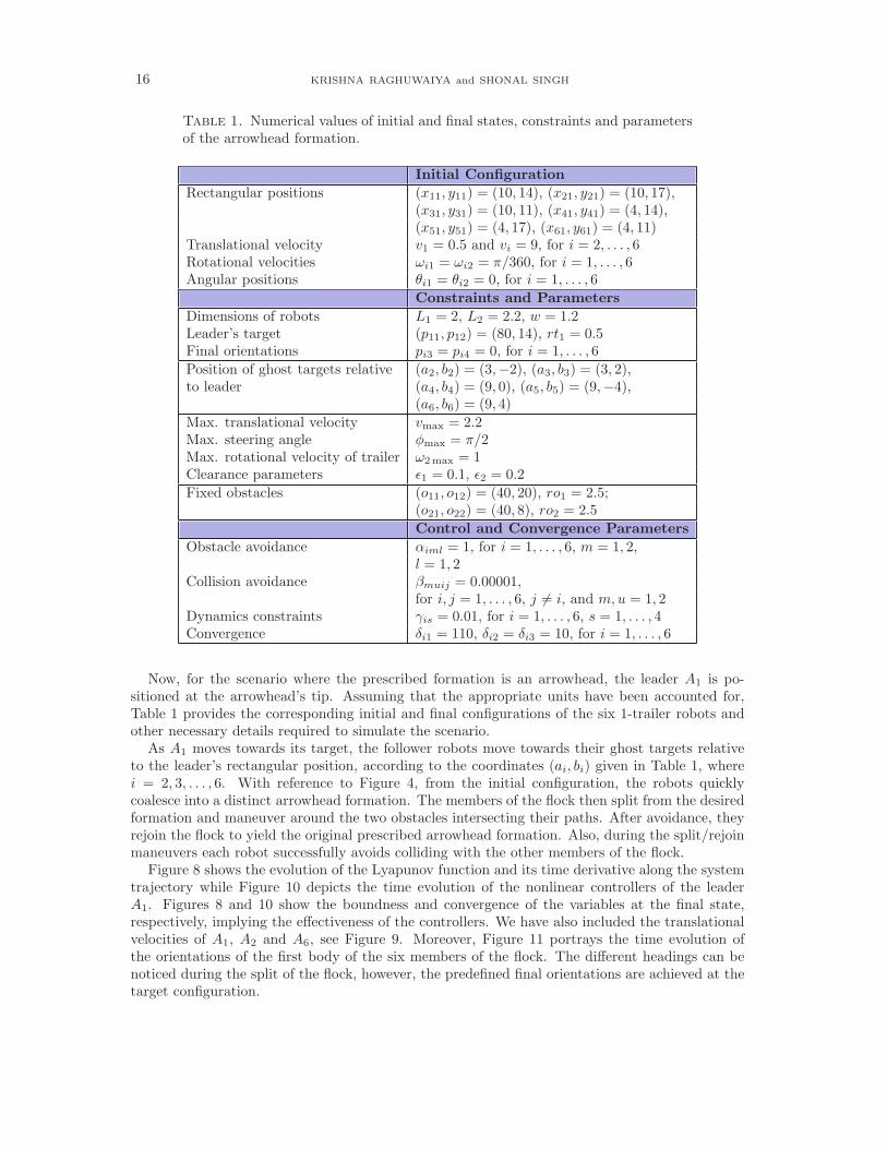
Table 1. Numerical values of initial and final states, constraints and parametersof the arrowhead formation.

Initial Configuration

Rectangular positions (x11, y11) = (10, 14), (x21, y21) = (10, 17),(x31, y31) = (10, 11), (x41, y41) = (4, 14),(x51, y51) = (4, 17), (x61, y61) = (4, 11)

Translational velocity v1 = 0.5 and vi = 9, for i = 2, . . . , 6Rotational velocities ωi1 = ωi2 = π/360, for i = 1, . . . , 6Angular positions θi1 = θi2 = 0, for i = 1, . . . , 6

Constraints and Parameters

Dimensions of robots L1 = 2, L2 = 2.2, w = 1.2Leader’s target (p11, p12) = (80, 14), rt1 = 0.5Final orientations pi3 = pi4 = 0, for i = 1, . . . , 6

Position of ghost targets relative (a2, b2) = (3,−2), (a3, b3) = (3, 2),to leader (a4, b4) = (9, 0), (a5, b5) = (9,−4),

(a6, b6) = (9, 4)

Max. translational velocity vmax = 2.2Max. steering angle φmax = π/2Max. rotational velocity of trailer ω2 max = 1Clearance parameters ǫ1 = 0.1, ǫ2 = 0.2

Fixed obstacles (o11, o12) = (40, 20), ro1 = 2.5;(o21, o22) = (40, 8), ro2 = 2.5

Control and Convergence Parameters

Obstacle avoidance αiml = 1, for i = 1, . . . , 6, m = 1, 2,l = 1, 2

Collision avoidance βmuij = 0.00001,for i, j = 1, . . . , 6, j 6= i, and m,u = 1, 2

Dynamics constraints γis = 0.01, for i = 1, . . . , 6, s = 1, . . . , 4Convergence δi1 = 110, δi2 = δi3 = 10, for i = 1, . . . , 6

Now, for the scenario where the prescribed formation is an arrowhead, the leader A1 is po-sitioned at the arrowhead’s tip. Assuming that the appropriate units have been accounted for,Table 1 provides the corresponding initial and final configurations of the six 1-trailer robots andother necessary details required to simulate the scenario.

As A1 moves towards its target, the follower robots move towards their ghost targets relativeto the leader’s rectangular position, according to the coordinates (ai, bi) given in Table 1, wherei = 2, 3, . . . , 6. With reference to Figure 4, from the initial configuration, the robots quicklycoalesce into a distinct arrowhead formation. The members of the flock then split from the desiredformation and maneuver around the two obstacles intersecting their paths. After avoidance, theyrejoin the flock to yield the original prescribed arrowhead formation. Also, during the split/rejoinmaneuvers each robot successfully avoids colliding with the other members of the flock.

Figure 8 shows the evolution of the Lyapunov function and its time derivative along the systemtrajectory while Figure 10 depicts the time evolution of the nonlinear controllers of the leaderA1. Figures 8 and 10 show the boundness and convergence of the variables at the final state,respectively, implying the effectiveness of the controllers. We have also included the translationalvelocities of A1, A2 and A6, see Figure 9. Moreover, Figure 11 portrays the time evolution ofthe orientations of the first body of the six members of the flock. The different headings can benoticed during the split of the flock, however, the predefined final orientations are achieved at thetarget configuration.


0 20 40 60 800

5

10

15

20

25

30

z1

z2

Initial ConfigurationDesired formation

is achieved

Leader

FO 1

FO 2

The flock splits

The flock rejoinsFinal Configuration

Target

FO: Fixed Obstacle

Figure 4. Arrowhead formation.

0 20 40 60 800

5

10

15

20

25

30

z1

z2


Desired formation

is achieved

Leader FO 1

The flock splits

The flock rejoins

and attains its final configuration

FO: Fixed Obstacle

Figure 5. Double platoon formation.

6. Conclusion

This paper presents a set of artificial potential field functions, derived from a Lyapunov-basedcontrol scheme, for the generation and advancement of a flock fixed in a prescribed formationof steerable 1-trailer nonholonomic robots via split/rejoin maneuvers. The advancement of theprescribed formation was from the inclusion of moving ghost targets positioned relative to theposition of the leader, a variant of the leader-follower strategy.

The continuous time-invariant acceleration controllers, derived within the framework of theLyapunov-based control scheme, generates split/rejoin maneuvers of the flock of 1-trailer mobile


0 20 40 60 800

5

10

15

20

25

30

z1

z2


Leader

Desired formation

is achieved

FO 1

FO 2

The flock splits

The flock rejoins Final Configuration

FO: Fixed Obstacle

Figure 6. Line formation.

0 50 100 1500

5

10

15

20

25

30

z1

z2


Desired formation

is achieved

Leader

The flock rejoins and attains

its final configuration

The flock splits

The disks represent

the fixed obstacles

Figure 7. Column formation.

robots in the vicinity of obstacles. The effectiveness of the proposed controllers was demonstratedvia computer simulations of different formation types, where the mobile robots operate within anobstacle-ridden environment. In each scenario, the derived controllers produced feasible trajec-tories and ensured a nice convergence of the system to its equilibrium state while satisfying thenecessary kinematic and dynamic constraints tagged to the mobile robots. We note here thatconvergence is only guaranteed from a number of initial states of the system.


0 2000 4000 6000 8000 10 000 12 000 14 000

0

1000

2000

3000

4000

5000

L(1)(x)

L(1)(x)

Time

Lyapunov

Functi

on

Figure 8. Behaviorof the Lyapunov func-tion L(1)(x) and itstime derivativeL(1)(x).

0 20 40 60 80 100 120 140-0.3

-0.2

-0.1

0.0

0.1

0.2

0.3

v1

v2

v6

Time

Velo

cit

ies

Figure 9. Evolutionof the translational ve-locities of A1, A2, andA6.

0 20 40 60 80 100 120 140

-0.06

-0.04

-0.02

0.00

0.02

0.04

0.06

σ11

σ12

σ13

Time

Contr

ollers

Figure

10. Evolution ofthe accelerationcomponents of A1.

0 20 40 60 80 100

-0.5

0.0

0.5

θ11

θ21

θ31

θ41

θ51

θ61

Time

Ori

enta

tions

Figure

11. Orientationsof the first solid bodyof the leader A1 andits followers.

Future research work includes applying the Lyapunov-based control scheme motion plannerto address the motion planning and control problem of flocks of steerable general tractor-trailersystems.

References

[1] A.P. Aguiar and A. Pascoal, Stabilization of the extended nonholonomic double integratorvia logic based hybrid control, In Proceedings of 6th International IFAC Symposium on RobotControl, Vienna, Austria, September 2000.

[2] F. Arrichiello. Coordination Control of Multiple Mobile Robots. PhD thesis, Universita DegliStudi Di Cassino, Cassino, Italy, November 2006.


[3] C. Bohm, M. Lazar, and F. Allgower, Stability analysis of periodically time-varying systemsusing periodic Lyapunov functions, In Proceedings of the IFAC Workshop on Periodic ControlSystems (PSYCO), Antalya, Turkey, 2010.

[4] R.W. Brockett, Differential Geometry Control Theory, chapter Asymptotic Stability andFeedback Stabilisation, Springer-Verlag, 1983, 181–191.

[5] L.G. Bushnell, D.M. Tilbury, and S.S. Sastry, Steeing chained form nonholonomic systemsusing sinusoids: The firetruck example, In The European Control Conference, Groningen, TheNetherlands, 1993, 1432–1437.

[6] L.G. Bushnell, D.M. Tilbury, and S.S. Sastry, Steering three-input nonholonomic systems: thefire truck example, The International Journal of Robotics Research, 14 (1995), 1428–1431.

[7] C. Cai, A.R. Teel, and R. Goebel, Smooth Lyapunov functions for hybrid systems part II:(Pre)asymptotically stable compact sets, IEEE Transactions on Robotics and Automation, 53(3) (2008), 734–748.

[8] D.E. Chang, S.C. Shadden, J.E. Marsden, and R. Olfati-Saber, Collision avoidance for mul-tiple agent systems, In Proceedings of the 42nd IEEE Conference on Decision and Control,Maui, Hawaii, USA, December 2003.

[9] Z. Chen, T. Chu, and J. Zhang, Swarm splitting and multiple targets seeking in multi-agentdynamic systems, In Proceedings of the 49th IEEE Conference on Decision and Control,Atlanta, GA, USA, December 2010, 4577–4582.

[10] D. Crombie. The Examination and Exploration of Algorithms and Complex Behavior to Re-alistically Control Multiple Mobile Robots, Master’s thesis, Australian National University.1997.

[11] W.E. Dixon, Z.P. Jiang, and D.M. Dawson, Global exponential setpoint control of wheeledmobile robots: a Lyapunov approach, Automatica, 36 (2000), 1741–1746.

[12] L. Edelstein-Keshet, Mathematical models of swarming and social aggregation, In Proceedings2001 International Symposium on Nonlinear Theory and Its Applications, Miyagi, Japan,October-November 2001, 1–7.

[13] E.F. Fukushima, S. Hirose, and T. Hayashi, Basic considerations for the articulated bodymobile robot, IROS 1998, 386–393.

[14] V. Gazi, Swarm aggregations using artificial potentials and sliding mode control, In Proceed-ings IEEE Conference on Decision and Control, Maui, Hawaii, December 2003, 2041–2046.

[15] Z.P. Jiang and H. Nijimeijer, Tracking control of mobile robots: a case study in backstepping,Automatica, 33 (7) (1997), 1393–1399.

[16] Z.P. Jiang, E. Lefeber, and H. Nijimeijer, Saturated stabilization and tracking of a nonholo-nomic mobile robot, Systems & Control Letters, 42 (2011), 327–332.

[17] W. Kang, N. Xi, J. Tan, and Y. Wang, Formation control of multiple autonomous robots:theory and experimentation, Intelligent Automation & Soft Computing, 10 (2) (2004), 1–17.

[18] F. Mnif and F. Touati, An adaptive control scheme for nonholonomic mobile robots withparametric uncertainty, International Journal of Advanced Robotic Systems, 2 (2005), 59–63.

[19] P. Ogren, Formations and Obstacle Avoidance in Mobile Robot Control, Master’s thesis, RoyalInstitute of Technology, Stockholm, Sweden, June 2003.

[20] R. Olfati-Saber and R.M. Murray, Flocking with obstacle avoidance: cooperation with limitedinformation in mobile networks, In Proceedings of the 42nd IEEE Conference on Decisionand Control, volume 2, Maui, Hawaii, USA, December 2003, 2022–2028.

[21] R. Olfati-Saber, Flocking of multi-agent dynamic systems: algorithms and theory, IEEETransactions on Automatic Control, 51 (3) (2006), 401–420.

[22] H. Prem and K. Atley, Performance evaluation of the trackaxle steerable axle system, InProceedings of the 7th International Symposium on Heavy Vehicle Weights and Dimensions,Delft, The Netherlands, June 2002.

[23] K. Raghuwaiya, S. Singh, B. Sharma, and J. Vanualailai, Autonomous control of a flockof 1-trailer mobile robots, In Proceedings of the 2010 International Conference on ScientificComputing, Las Vegas, USA, July 2010, 153–158.


[24] W. Ren, R. Beard, and E. Atkins, Information consensus in multivehicle cooperative control:collective group behavior through local interaction, International Journal of Robotics Research,27 (2) (2007), 71–82.

[25] S. Samson, Time-varying feedback stabilisation of car-like wheeled mobile robots, InternationalJournal of Robotics Research, 12 (1) (1993), 55–64.

[26] B. Sharma and J. Vanualailai, Lyapunov stability of a nonholonomic car-like robotic system,Nonlinear Studies, 14 (2) (2007), 143–160.

[27] B. Sharma, J. Vanualailai, K. Raghuwaiya, and A. Prasad, New potential field functions formotion planning and posture control of 1-trailer systems, International Journal of Mathemat-ics and Computer Science, 3 (1) (2008), 45–71.

[28] B. Sharma, New Directions in the Applications of the Lyapunov-based Control Scheme to theFindpath Problem. PhD thesis, The University of the South Pacific, Suva, Fiji Islands, July2008.

[29] B. Sharma, J. Vanualailai, and U. Chand, Flocking of multi-agents in constrained environ-ments, European Journal of Pure and Applied Mathematics, 2 (3) (2009), 401–425.

[30] Z. Song, D. Zhao, J. Yi, and X. Li, Robust motion control for nonholonomic constrained me-chanical systems: sliding mode approach, In Proceedings of the American Control Conference,June 2005, 2883–2888.

[31] J. Vanualailai, J. Ha, and S. Nakagiri, A collision and attraction problem for a vehicle, InRIMS Symposium, Kyoto University, Japan, November 2003.

[32] J. Vanualailai and B. Sharma, Moving a robot arm: an interesting application of the directmethod of Lyapunov, CUBO: A Mathematical Journal, 6 (3) (2004), 131–144.

[33] T. Vidal-Calleja, M. Velasco, and E. Aranda, Artificial potential fields for trailer-like systems,In X Congreso Latinoamericano de Control Automtico, Guadalajara, Mxic, November 2002,1–6.

[34] Q. Wang, H. Fang, J. Chen, Y. Mao, and L. Dou, Flocking with obstacle avoidance and con-nectivity maintenance in multi-agent systems, In Proceedings IEEE 51st Annual Conferenceon Decision and Control, Decemeber 2012, 4009–4014.

[35] J. Wen, Control of Nonholonomic systems. March 31 1998.[36] X. Xin, T. Mita, and M. Kaneda, The psoture control of a 2-link free flying acrobot with initial

angular momentum, In Proceedings of the 41st IEEE Conference on Decision and Control,Las Vegas, Nevada, USA, December 2002, 2068–2073.

[37] Z. Xue, Z. Liu, C. Feng, and J. Zeng, Target tracking for multi-agent systems with leader-following strategy, In Proceedings of the third International Symposium on Electronic Com-merce and Security Workshops, Guangzhou, China, July 2010, 240–243.

Krishna RaghuwaiyaThe University of the South PacificSuva,Fiji

[email protected]

Shonal SinghThe University of the South PacificSuva,

Fiji

formation types of multiple steerable 1-trailer mobile robots via split

Documents