fourier methods of seismic data regularisationsep · fourier methods of seismic data regularisation...

Fourier methods of seismic data regularisation

Chris Leader and Sjoerd de Ridder

ABSTRACT

Acquisition geometries of seismic data invariably lead to an irregular sampling inspace of midpoint, offset and azimuth, however many seismic processing theoriesand algorithms work best if not exclusively on regularly sampled data. Here,three methods of Fourier regularisation are implemented and contrasted eachwith their own benefits and drawbacks. Standard theory is extended to the useof discrete spheroidal prolate sequence multitapers to help to diminish spectralcontamination caused by an irregular input grid. Early results show that theuse of multitapers alone have not yet proved to adequately reconstruct the inputdata, however the use of these to augment other types of Fourier regularisationhave shown promise in increasing accuracy and reducing the number of requirediterations.

INTRODUCTION

Regularisation of input data is required, or at least assumed, for a variety of ad-vanced seismic data processing methods. Consequently if the input data is irregu-larly sampled then the effectiveness of many methods are compromised. Particularlyalgorithms such as 3D surface related multiple elimination (SRME) and pre-stackwave-equation depth migration have been shown to suffer considerably when appliedto irregular data, and often induce new processing artifacts (Canning and Gardner,1996). Furthermore irregular sampling can also lead to poor repeatability between4D seismic surveys (at least for conventional 4D processing). To help alleviate theseproblems a common seismic data processing step involves some form of regularisationand/or interpolation.

Whilst precise definitions can vary, the concept of regularisation involves transfer-ring samples from their irregular input grid to new locations on a regular output grid.Often interpolation will follow regularisation, whereby missing samples in the outputgrid are filled in; this is also often used to interpolate to a finer grid. A regularisationoperator that can handle aliased and non-stationary events is desired, as this willassist in the preservation of all signal.

Several advanced regularisation methods have been suggested to overcome theproblem of irregularly sampled data. One such technique is to use convolution opera-tors known as prediction error filters (PEFs) that can predict absent traces honouring

SEP–140

Leader and de Ridder 2 ALFT and Slepian tapers

the spectra of known traces, however this can be limited due to an assumption of locallinearity (Abma, 1995). As discussed in Biondi (2005) the problem can also be solvedby AMO regularisation, whereby data is reconstructed at an arbitrary (regular) az-imuth.

Fourier based methods can also be used, where the regularisation is performedby preserving the spectrum of the data and inverse transforming to a desired grid;however this suffers from the phenomena known as spectral leakage. The problemarises due to the non-orthogonality of the global basis functions (the sinc function)that are exhibited by an irregular grid (Xu and Pham, 2004a) and is discussed indetail in the next section. This phenomenon has been addressed by many disciplinesthat involve time series analysis, and several solutions to remove or reduce spectralleakage have been created.

A further possibility is to design an appropriate taper to minimise spectral leakageabout a certain frequency or band of frequencies, and these are known as Slepiantapers, as discussed in Slepian (1978) and Percival and Walden (1993). The conceptis that the taper parameters are designed to maximise spectral concentration within apredefined resolution bandwidth window, and so the use of these should help to greatlyreduce the number of iterations required in other Fourier regularisation methods, orpossibly replace them altogether. Such methods have been shown to work on randomsignals, synthetic earthquake signals and for bathymetry profiles (Prieto, 2007), andso the extension of this concept to active seismic data could help the solve the problemof Fourier regularisation.

SPECTRAL LEAKAGE

The occurence of spectral leakage is a fundamental product of data reconstructiontheory, which can be summarised to say that if a coninuous function is sampled byat least the Nyquist interval, such that ∆t ≤ π/ωNy, then total reconstuction ofthe input series is completely determined. However a fundamental assumption ofthis theory is that the basis functions used for reconstruction are orthogonal, and tosummarise this assumption can be described as

〈ϕk, ϕl〉 =

∫ ∞

−∞sinc(

x

T− k)sinc(

x

T− l) dx, (1)

= sinc(k − l) = δkl (2)

where δkl is the Kronecker delta function and k, l are integers (Xu and Pham, 2004b).On a regular grid this ensures that the sinc function has value 1 on the original dataposition, and 0 elsewhere. However, on an irregular grid this condition is violated,and indeed the Nyquist concept is less meaningful. The non-orthoganality of these

SEP–140


basis functions leads to a non-orthogananilty of Fourier coefficients, and this causesenergy from large Fourier coefficients to ‘leak’ to others in the frequency domain,resulting in a denser, noisier spectrum. An example of this can be seen in Figure 2.

In light of fact that for real data there is always irregularity, whether it is dueto cable feathering, obstacles or statics, Fourier regularisation methods must try andreduce or remove spectral leakage. To do this an irregular Fourier transform, itsinverse and an appropriate weighting scheme must be devised.

IRREGULAR FOURIER TRANSFORM

The regular unitary discrete Fourier transform can be expressed as follows

F (k) =1√N

N−1∑l=0

f(xl) e−2πikxl , k = 0,±1,±2, ...,±N (3)

where F (k) denotes the size of the kth Fourier coefficient, xl is the position of theinput data and f(xl) denotes the value of the input data series corresponding to thisposition. To extend this expression to handle an irregular xl series we must definea new transform, and care must be taken with the transform weights to ensure theforward and inverse transforms are unitary; this is simply done by dividing by

√N

in the regular case.

The weights must be related to the relative positioning of xl on the input axis,with some form of normalisation. This can be done by letting

F (k) =1√N

N−1∑l=0

f(xl)∆xl

∆xav

e−2πikxl , (4)

=1√N

N−1∑l=0

1

∆xav

N−1∑l=0

f(xl)∆xl e−2πikxl , (5)

=

√N

∆X

N−1∑l=0

f(xl)∆xl e−2πikxl , (6)

∆X is the range of the input axis, xN − x1. The weighting here has taken intoaccount the data range, size, and relative irregularity. Upon multiple tests it is easyto show that this transform is indeed unitary, and corretly preserves amplitudes afterhundreds of domain transformations. The ∆xl values are calculated using a symmetricdifferencing star for stability, such that

∆xl =1

2(xl+1 − xl−1) (7)

SEP–140


a weighting scheme for applying the transform in multiple dimensions is more diffi-cult to estimate, but the problem can be broken down and each dimension consideredseparately for this application.

However designing an appropriate weight does not alleviate spectral leakage. Onefirst method used was setting up the problem as a least squares inverse, using theCauchy norm of F (k) as a regularisation term within the cost function (Saachi andUlrych, 1995), however a key problem with this approach was that the data is notsufficiently honoured.

ANTI-LEAKAGE FOURIER TRANSFORM

The first documented solution to the leakage problem was performed by Hogbom(1974) as a solution within Astrophysics. The situation was similar to that of seismicdata regularisation - radio interferometric baselines after aperture synthesis did notfall on a regular grid as desired, and the adaptive process known as ‘The CLEANAlgorithm’ was devised.

An adaptation of this can give a robust solution to Fourier regularisation, as dis-cussed by Xu and Pham (2004a), Xu and Pham (2004b) and Schonewille (2009), andhas been named the ‘anti-leakage Fourier transform’ due to its ability to suppressspectral leakage. This is an iterative algorithm, which exploits the fact that leakageis caused by high energy components contaminating other Fourier components. Themaximum component of a given spectrum is calculated and added to an ‘estimated’spectrum, then the contribution of this component is removed from the input datain data space, by inverse transforming the single component (taking care to recon-struct the same irregular axis) and subtracting. The new spectrum will see this peakremoved, and then the next highest energetic component is found, added to the esti-mated spectrum and removed from the input data, and then iterations continue. Thenumber of iterations is problem dependent, but the maximum required to rebuild aleakage free spectrum will be N , the number of Fourier components, and often farfewer will be required. The final spectrum is free of leakage, however some attentionmust be paid to Fourier artifacts; in this case cosine tapering is applied to the edgesof the data

This algorithm can be summarised as follows

1. Compute the irregular, weighted DFT of the input data

2. Select the strongest Fourier component

3. Add this value to the estimated spectrum

4. Inverse irregular DFT this component (onto the irregular input axis)

SEP–140


5. Subtract this component from the input data

6. Iterate until the desired number of Fourier components have been estimated

It is clear from this set up that this algorithm is very limited by problem size. If theinput axis is of length N and Nk components are to be estimated then O(NxNxNk)operations are required. Weights are only axis dependent so these are calculated andstored outside of the main loop.

One Dimensional Example

The power of the ALFT is best observed using a 1-D example and examining how theinput series and corresponding spectra evolve with iterations. A 1-D irregular axis isconstructed, where the irregularity is limited to half a bin size about the corresponding‘regular’ position such that x(ix) = ox + (ix − 1) ∗ dx + (rand − 0.5) ∗ dx, where ixin the position index, ox an arbitrary origin, dx the receiver/trace spacing and randa random number between 0 and 1. This is representative of the problem for landdata.

Using this axis a superposition of sine waves is created of varying frequencies,amplitude and phase. For the presented example two different waves are used forviewing simplicity.

Figure 1: Part of the irregularlysampled sine wave superpositionused as input data/ [ER]

As can be seen in Figure 3 the ALFT has perfectly reconstructed a regular signalfrom the irregular input, and the spectrum is free from leakage except for adjacentto the main peaks. In this oversimplified example only four iterations are reallyrequired. Also note the amplitude preservation between Figure 2 and Figure 3. Forfurther insight a more complicated, higher dimensional example is required.

SEP–140


Figure 2: A section of the DFT reconstructed sine wave and its corresponding spec-trum. [ER]

Figure 3: A section of the ALFT reconstructed sine wave and its correspondingspectrum. [ER]

SEP–140


Two Dimensional Plane Wave Example

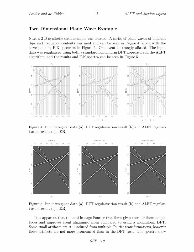
Next a 2-D synthetic data example was created. A series of plane waves of differentdips and frequency contents was used and can be seen in Figure 4, along with thecorresponding F-K spectrum in Figure 6. One event is strongly aliased. The inputdata was regularised using both a standard nonuniform DFT approach and the ALFTalgorithm, and the results and F-K spectra can be seen in Figure 5

Figure 4: Input irregular data (a), DFT regularisation result (b) and ALFT regular-isation result (c). [ER]

Figure 5: Input irregular data (a), DFT regularisation result (b) and ALFT regular-isation result (c). [ER]

It is apparent that the anti-leakage Fourier transform gives more uniform ampli-tudes and improves event alignmnet when compared to using a nonuniform DFT.Some small artifacts are still induced from multiple Fourier transformations, howeverthese artifacts are not more pronounced than in the DFT case. The spectra show

SEP–140


Figure 6: FK Spectra of the input data (a), data with DFT regularisation (b) anddata with ALFT regularisation (c). [ER]

that most of the incoherent noise in the ALFT regularised image is induced fromthe aliased event, giving a mostly clean spectrum elsewhere. Wrongly dipping eventsand noise in the corresponding DFT spectrum is significantly reduced in the ALFTspectrum.

QDome Data Example

To use a more realistic seismic example the QDome synthetic data from Claerbout’sImage Estimation By Example (Claerbout, 1995) was adapted to contain an irregu-lar x-axis, details of the data computation can be found in Claerbout (1995). Thisdataset features flat beds at the surface, a Gaussian centre with a fault and dippingbeds at the bottom - this model is useful since it incorporates events that are flat,dipping, curving, aliased and discontinuous, and so is an appropriate model to testthe robustness of the algorithm.

An irregular axis was created as in the previous examples and the QDome datawas calculated for this irregular axis. A 3D cube of data was created and presentedherein are two slices from the cube orthogonal to the (regular) y axis - one slice con-taining strongly aliased events and one containing a discontinous fault

The ALFT shows a much improved result in both of these cases. In this examplethe DFT particularly struggles with the amplitudes of the traces and some appearmuch diminished - these are the traces that were the most irregular. The fault appearsmore continuous and defined in the ALFT result than in the irregular input image,as do the steep events in Figure 8. However the algorithm still struggles somewhat

SEP–140


Figure 7: QDome slice containing aliased data (a), DFT regularisation result (b) andALFT regularisation result (c). [ER]

Figure 8: QDome slice containing a fault (a), DFT regularisation result (b) and ALFTregularisation result (c). [ER]

SEP–140


in the aliased sections of the data, and the spectrum (as seen in Figure 7), is noisierin aliased regions. Schonewille (2009) discusses how this problem can be addressed,and this can be done by extrapolating the known spectrum to higher ω and k values,estimating weights for these higher frequencies and computing the ALFT for these.

Whilst the results of using the ALFT show a marked improvement over DFTregularisation and a robustness in the presence of aliased and discontinuous eventsit is fundamentally limited by its reliance on multiple domain transformations. Forlarge datasets the number of operations required by this technique is unreasonableand so a different method, or maybe one that augments the ALFT to require fewertransforms, is desired. It is possible that the answer to this problem lies in taperingthe input data in such a way that Fourier components can be made more orthogonal.This is discussed in the subsequent section.

SLEPIAN TAPERS

Equation 6 can be slightly modified to include a new series of weights, or tapers,a(xl),

Fw(k) =

√N

∆X

N−1∑l=0

f(xl)aw(xl)∆xl e−2πikxl , (8)

if a(xl) is a boxcar then equation 8 will reduce to 6. It is possible to design a seriesof tapers a(xl) in order to reduce spectral leakage, and this is a classical time seriesanalysis solution. Each w subscript indicates a possible different taper.

Thomsen (1982) proposed the multitaper method, which is now widely used ingeophysical applications. In this method a(xl) represents a set of orthogonal tapersthat can be averaged over to give an estimation of the power spectral density func-tion (the absolute value squared of the Fourier sequence.) This can outperfrom usinga single taper method for several reasons; one being that using a single taper candiscard a significant amount of the signal. When using the multitaper method this isless of a problem since information discarded by one taper can be (at least partially)recovered by the others (Prieto, 2007).

Slepian (1978) showed that by stipulating a requirement of spectral leakage min-imisation the design of the tapers becomes an eigenfunction problem. Ultimately theend result resembles

Da− λa = 0, (9)

where D is the matrix desrcibed by:

SEP–140


Dn,m =sin 2πW (n−m)

π(n−m)n, m = 0, 1, 2, ...N − 1, (10)

where W is a predefined resolution bandwidth such that 1 < NW < N/2, and NW isknown as the time bandwidth product (or the number of Rayleigh bins) and controlsthe amount of smoothing in the frequency domain. λ here represents a measure ofspectral concentration and a the set of eigenfunctions associated with (4), which willbe the components of the multitaper estimate (Percival and Walden (1993)). Thecloser that λ is to 1 then the greater the expected suppression of spectral leakage is,and indeed 1− λ is a good measure of taper ’strength’ and will be a core componentof the weighting scheme used. The resulting sequence of tapers are known as Slepiantapers, or Discrete Prolate Spheroidal Sequences (DPSSs), each DPSS is dependenton the choice of NW. The first four tapers in the sequence NW=4 are shown in Fig-ure 9.

Figure 9: The first 4 Slepian tapers calculated with NW=4, also known as the 4πSlepian sequence. [ER]

Using a very similar method Prieto (2007) showed that this can be effective indetermining and quantifying the spectra of earthquake and bathymetry data. Whilstit is true that estimating the tapers from the data is computationally intensive, onceestimated the tapers are stored and reused (if iterations are required,) and so a sub-stantially improved run time relative to the ALFT is shown.

As can be seen from Eq. (5) the matrix D is dense and symmetric. This symmetryexists because the matrix can be rewritten as Dn,m = 2W sinc 2πW (n−m) and thesinc function is symmetric. The eigenfunctions need to be found and so D is reduced

SEP–140


to tridiagonal form using Householder’s reduction. Then using QL decompositionthe eigenvalues and eigenvectors of this real, symmetric, tridiagonal matrix can becomputed and hence the tapers calculated (Sparks and Todd, 1973).

However the manner in which these tapers are computed does not easily lead tocalculating the tapers over an irregular grid, and since the tapers are applied withinthe forward Fourier transform kernel they must lie on the same grid as the input data.This problem can be solved be creating a very dense taper and then subsampling tothis to the input transformation axis. Moreover this process is made more accurateby linearly interpolating the irregular taper value between the two known values onthe dense grid. Since the tapers only require calculating once for a given time serieslength and time bandwidth product, creating a dense series of tapers does not causeany significant computation time.

One issue that requires much thought is the design of weighting functions for theprocedure that will not cause local bias within the data. A well designed weightingfunction will generate a smooth estimate from the mutlitaper scheme, with less vari-ance than the corresponding single taper method and also will try and reduce anylocal bias. Several methods have been suggested such as that by Thomsen (1982),Riedel and Sidorenko (1995) and Prieto (2007). The method used herein follows thederivation by Thomsen, where the taper weights are frequency dependent and arecalculated using λ.

|F (k)|2 =

N−1∑w=0

d2k|Fw(k)|2

N−1∑w=0

d2k

, (11)

dw(k) =

√λk|Fw(k)|2

λk|Fw(k)|2 + (1− λk)σ2(12)

(13)

where as before Fw(k) the result of Fourier transforming the product of the inputseries with the taper aw, λ is the eigenvalue of the given taper and σ is the varianceof the input series. This can be proved by seeking to estimate the discrepency of thedifferent eigencomponents, Fw(k), and an involved proof can be seen in Percival andWalden (1993).

These classical weights are designed for weighting the power spectral density func-tion (PSD), which is the square of the amplitudes of the spectrum. However in takingthe power of the spectrum the phase information is lost, and so the phase spectrumis computed and stored before the PSD is computed and weighted, and now theweighted spectrum can be (roughly) estimated by combining the root of the powerwith the unweighted phases.

SEP–140


Results using Slepian tapers

The use of Slepian tapers for seismic data regularisation requires some initial inge-nuity, since previously their purpose has been in estimating the spectra of complexprocesses and not in reconstructing data. Figure 10 shows a windowed irregular spec-trum containg two main frequencies and its equivalent spectrum after applying four πSlepian tapers and weighting appropriately. The irregular spectum indicates leakagehas occured, both around the peak and at higher frequencies, whilst the spectrum af-ter tapering shows less contamination around the frequencies of interest and an overlycleaner spectrum. In this case the tapering has reduced the spectral leakage with lit-tle computation time. It should be noted that the ALFT can often not remove theleaked frequencies surrounding the main peaks, whilst the DPSS tapers have reducedthis.

Figure 10: The result of applying the four tapers in the π DPSS sequence to aspectrum exhibiting leakage. [ER]

The choice of number of tapers and the time bandwidth product is very situationdependent. In a lot of cases a poor choice of the time bandwidth product merely servesthe smear spectral peaks and enhance leakage, even giving zero frequency energies.

The taper weights are designed to reduce the bias of the power spectrum, and notthe amplitude. Using these weights on the amplitude gives peak splitting, which the-ory tells us should happen, and if the root of the power is used then phase informationof the data is lost. Ongoing efforts involve calculating amplitude and/or phase weightsto reduce bias, rather than within the power. Currently in data reconstruction taperimprints are still visible, which again was expected by theory. Increasing the numberof tapers alters this problem, and a method of amplitude preservation is yet to befinalised. Currently the method outlined by Park (1992) where the reconstruction isposed as an inverse problem is being attempted.

SEP–140


CONCLUSIONS

This paper has shown that Fourier methods of seismic data regularisation can be apowerful and robust method in regularising data, which is useful for future processingsteps and for image viewing. A standard irregular DFT has limited application sincethe contaminated spectra lead to a large number of artifacts and amplitudes are notreconstructed correctly. Using a recursive ALFT approach gives a much improvedresult - amplitudes are now correct along events, events are exactly aligned in thecorrect places and there is a slight reduction in artifacts. Discontinuous events areimaged and whilst aliased events are not perfectly reconstructed they do not contam-inate the image as strongly as in the standard DFT case, and this method can beextended to handle these sorts of frequencies. However the ALFT approach is slow,and could be improved by implementing a non-uniform FFT and better taperingbetween transforms, to help reduce artifacts.

Examination of multitaper methods with Slepian tapers has yielded some intrigu-ing results - the spectra after tapering and stacking are shown to have reduced spec-tral leakage without iterations around frequencies of interest, however leakage noiseat higher frequencies is preserved.

Key issues that still require resolving before this is proved to be a viable reg-ularisation method are those of adapting taper weights to optimise the amplitudespectrum and not the power, a better method of reconstructing and weighting thephase spectrum and a more robust method of removing the taper imprints in thereconstruced data. Early tests are showing that these problems are gradually beingovercome.

ACKNOWLEDGMENTS

I would like to thank Jim Berryman for his insightful discussions about spectral tapersand his useful literary recommendations.

REFERENCES

Abma, R, C. J., 1995, Lateral prediction for noise attenuation by t-x and f-x tech-niques: Geophysics, 60, 1887–1896.

Biondi, B., 2005, 3d seismic imaging: Society of Exploration Geophysicists.Canning, A. and G. Gardner, 1996, Another look at the question of azimuth: The

Leading Edge, 15, 821–823.Claerbout, J., 1995, Image estimation by example: Society of Exploration Geophysi-

cists.Hogbom, J., 1974, Aperture synthesis with a non-regular distribution of interferom-

eter baselines: Astronomy and Astrophysics, 15, 417–426.

SEP–140


Park, J., 1992, Enevlope estimation for quasi-periodic geophysical signals in noise: amultitaper approach: Edward Arnold, London.

Percival, D. and A. Walden, 1993, Spectral analysis for physical applications: Cam-bridge University Press.

Prieto, G. e. a., 2007, Reducing the bias of multiptaper spectrum estiamtes: Interna-tional Journal of Geophysics, 171, 1269–1281.

Riedel, K. and A. Sidorenko, 1995, Mimimum bias multiple taper spectral estimation:IEEE Transactions on Signal Processing, 43, 188–195.

Saachi, M. and T. Ulrych, 1995, High-resolution velocity gathers and offset spacereconstruction: Geophysics, 60, 1169–1177.

Schonewille, M. e. a., 2009, Sesimic data regularisation wtih the anti-alias anti-leakagefourier transform: The First Break, 27, 85–92.

Slepian, D., 1978, Prolate, spheroidal wavefunctions, fourier analysis and uncertaintyv: the discrete case: Bell System Technical Journal, 57, 1371–1430.

Sparks, D. and A. Todd, 1973, Latent roots and vectors of a symmetric matrix:Applied Statistics, 22, 260–265.

Thomsen, D., 1982, Spectrum estimation and harmonic analysis: Procedings of theIEEE, 70, 1055–1096.

Xu, S. and D. Pham, 2004a, Seismic data regularisation with anti-leakge fouriertransform: EAGE 66th Conference and Exhibition.

Xu, S, Z. Y. and D. Pham, 2004b, On the orthogonality of anti-leakage fourier trans-form based sesimic trace interpolation: SEG Int’l Exposition and 74th AnnualMeeting.

SEP–140

16

SEP–140 271

Mandy Wong graduated in 2004 with a B.Sc. in Physics andMathematics from the University of British Columbia (UBC) inVancouver, Canada. In 2006, she obtained a M.Sc. degree inCondensed Matter Thoery at UBC. Afterward, Mandy workedfor a geophysical consulting company, SJ Geophysics, based inVancouver, Canada. Mandy joined SEP in 2008, and is workingtowards a Ph.D. in Geophysics. Her main research interest isimaging with multiples.

Yang Zhang graduated from Tsinghua University in July 2007with a B.E. in Electrical Engineering. He took an internship inMicrosoft Research Asia during 2007-2008. He joined SEP in2009, and is currently pursuing a Ph.D. in Geophysics.

fourier methods of seismic data regularisationsep · fourier methods of seismic data regularisation...

Documents