FPBH.jl: A Feasibility Pump Based Heuristic forMulti-objective Mixed Integer Linear Programming in Julia

Aritra Pal and Hadi Charkhgard

Department of Industrial and Management System Engineering, University of SouthFlorida, Tampa, FL, 33620 USA

September 8, 2017

Abstract

Feasibility pump is one of the successful heuristic solution approaches developed almost adecade ago for computing high-quality feasible solutions of single-objective integer linear pro-grams, and it is implemented in exact commercial solvers such as CPLEX and Gurobi. In thisstudy, we present the first Feasibility Pump Based Heuristic (FPBH) approach for approximatelygenerating nondominated frontiers of multi-objective mixed integer linear programs with an ar-bitrary number of objective functions. The proposed algorithm extends our recent study forbi-objective pure integer programs that employs a customized version of several existing algo-rithms in the literature of both single-objective and multi-objective optimization. The methodhas two desirable characteristics: (1) There is no parameter to be tuned by users other thanthe time limit; (2) It can naturally exploit parallelism. An extensive computational study showsthe efficacy of the proposed method on some existing standard test instances in which the truefrontier is known, and also some randomly generated instances. We also numerically show theimportance of parallelization feature of FPBH and illustrate that FPBH outperforms MDLS de-veloped by Tricoire [39] on instances of multi-objective (1-dimensional) knapsack problem. Wetest the effect of using different commercial and non-commercial linear programming solvers forsolving linear programs arising during the course of FPBH, and show that the performance ofFPBH is almost the same in all cases. It is worth mentioning that FPBH is available as an opensource Julia package, named as ‘FPBH.jl’, in GitHub. The package is compatible with the pop-ular JuMP modeling language (Dunning et al. [16] and Lubin and Dunning [27]), supports inputin LP and MPS file formats. The package can plot nondominated frontiers, can compute differ-ent quality measures (hypervolume, cardinality, coverage and uniformity), supports execution onmultiple processors and can use any linear programming solver supported by MathProgBase.jl(such as CPLEX, Clp, GLPK, etc).

Keywords. Multi-objective mixed integer linear programming, feasibility pump, local search,local branching, parallelization

1

1 Introduction

Multi-objective optimization provides decision-makers with a complete view of the trade-offs betweentheir objective functions that are attainable by feasible solutions. It is thus a critical tool in engineer-ing and management, where competing goals must often be considered and balanced when makingdecisions. For example, in business settings, there may be trade-offs between long-term profits andshort-term cash flows or between cost and reliability, while in public good settings, there can betrade-offs between providing benefits to different communities or between environmental impacts andsocial good. Especially when such trade-offs are difficult to make, enabling decision-makers to see therange of possibilities offered by the nondominated frontier (or a portion of the nondominated frontier),before selecting their preferred solution, can be highly valuable. Combined with the fact that manyengineering problems can be formulated as mixed integer linear programs, the development of efficientand reliable multi-objective mixed integer linear programming solvers may have significant benefitsfor problem solving in industry and government.

In recent years, several studies have been conducted on developing exact algorithms for solvingmulti-objective optimization problems, see for instance Dachert et al. [13], Dachert and Klamroth[14], Kirlik and Sayın [23], Koksalan and Lokman [24], Ozlen et al. [29], Przybylski and Gandibleux[33], Przybylski et al. [34], Soylu and Yıldız [38], and Boland et al. [5, 6, 7]. This resurgence of intereston exact solution approaches for solving multi-objective optimization problems in the last decade ispromising. However, there is still a large proportion of multi-objective optimization problems thateither no exact method is known for them (such as mixed integer linear programs with more than twoobjective functions) or exact solutions approaches cannot solve them in reasonable time (for example,large size instances of NP-hard problems).

Consequently, developing heuristic solution approaches for multi-objective optimization problemsis worth studying. We note that in the last two decades, significant advances have been made ondeveloping evolutionary methods for solving multi-objective optimization problems. A website main-tained by Carlos A. Coello Coello (http://delta.cs.cinvestav.mx/~ccoello/EMOO/), for example,lists close to 4,700 journal papers and around 3,800 conference papers on the topic (inducing but notlimited to [10, 12, 15, 19, 25, 28, 40]).

Surprisingly, most of these methods are not specifically designed for problems with integer decisionvariables. Even if they can directly handle integer decision variables, they are often problem-dependentalgorithms. This means that they are usually designed for solving a certain class of optimizationproblems, for example, multi-objective facility location problem. Moreover, many of the existinggeneric heuristics are designed to solve unconstrained multi-objective optimization problems. So, ifthere are some constraints in the problem, these methods will usually remove them by penalizing themand adding them to the objective functions.

In light of the above, the literature of multi-objective mixed integer programming is sufferingfrom the lack of studies on generic heuristic approaches. Three of very few studies in this scope areconducted by Tricoire [39], Lian et al. [26] and Paquete et al. [32]. In these studies, two successfulheuristics, the so-called Multi-Directional Local Search (MDLS) and Pareto Local Search (PLS), aredeveloped that can solve multi-objective pure integer linear programs. We note that, these methodshave been shown to be successful in practice, but they have two main weaknesses: (1) It is not clearwhether they can handle mixed integer linear programs with multiple objectives since they are notspecifically designed to do so; (2) Users have to customize these algorithms to be able to solve theirspecific problems. In other words, only the framework of these algorithms is generic.

2

In this study, we develop an algorithm that overcomes both of these weaknesses. The proposedheuristic is generic, easy-to-use, and can approximate the nondominated frontier of any multi-objectivemixed (or pure) integer linear program with an arbitrary number of objective functions. The proposedmethod has two other desirable characteristics as well. (1) There is no parameter to be tuned by usersother than the time limit. (2) It can naturally exploit parallelism.

The engine of the proposed algorithm is basically the well-known feasibility pump heuristic [3, 20,1, 8, 22]. The feasibility pump is one of the successful heuristic solution approaches that developedjust a decade ago for solving single-objective mixed integer linear programs. The approach is sosuccessful and easy-to-implement that quickly after its invention it found its way into commercialoptimization solvers such as CPLEX and Gurobi. Consequently, the main motivation of our study isthat developing a similar technique for multi-objective mixed integer linear programs may follow thesame path in the future.

This is highlighted by the fact in our recent study, we developed a feasibility pump based heuris-tic for solving bi-objective pure integer linear programs (see Pal and Charkhgard [31]), and obtainpromising computational results. So, in this study, we extend our previous work to multi-objectivemixed integer linear programs with an arbitrary number of objective functions. The algorithm de-veloped, in our previous study, combines the underlying ideas of several exact/heuristic algorithmsin the literature of both single and multi-objective optimization including the perpendicular searchmethod [11, 4], a local search approach [39], and the weighted sum method [2] as well as the feasi-bility pump. Although our new method inherit the key components of our previous study, but it iscompletely different and novel. The following are some of the main differences:

• In the new method, the underlying idea of another well-known technique, the so-called localbranching [21], is also added to the algorithm. This is motivated by the observation that localbranching can align well with the feasibility pump for single-objective optimization problems[36]. In this study, we show that the same observation is true for multi-objective optimizationproblems as well.

• The weighted sum method used in the previous study does not work for instances with morethan two objectives. So, we develop a different weighted sum method for those instances.

• The underlying decomposition technique of the perpendicular search method used in the previousstudy does not work for problems with more than two objectives. So, in this study, we employa different but effective decomposition technique that does not dependent on the number ofobjective functions.

• The local search method developed in the previous study is used in this study as well. However,in addition to that, we develop a new local search technique that should be activated if thereexist continuous variables in an instance.

We conduct an extensive computational study that has three parts. In the first part, we test ouralgorithm on bi-objective mixed integer linear programs. In the second part, the performance of thenew algorithm is tested on multi-objective pure integer programs. Finally, in the third part, a set ofexperiments is conducted to show the performance of the algorithm on mixed integer linear programswith more than two objectives. In each of these parts, the importance of different components ofthe algorithm as well as its parallelization feature are shown. Furthermore, in each part, the effect

3

of using different linear programming solvers, including CPLEX, GUROBI, SCIP, GLPK and Clp, atthe heart of the proposed algorithm is illustrated. It is shown that the proposed algorithm performsalmost the same with any of these solvers. Finally, since the implementation of MDLS developed for(1-dimensional) knapsack problem is publicly available, we compare the performance of our algorithmagainst MDLS on some existing instances for this class of optimization problem, and show that ouralgorithm performs better.

The remainder of the paper is organized as follows. In Section 2, we introduce notation and somefundamental concepts. In Section 3, we provide the general framework of our algorithm. In Section 4,we introduce the proposed weighted sum operation. In Section 5, we introduce the proposed feasibilitypump operation. In Section 6, the proposed local search operation is explained. In Section 7, weconduct an extensive computational study. Finally, in Section 8, we give some concluding remarks.

2 Preliminaries

A multi-objective mixed integer linear program (MOMILP) can be stated as follows:

min(x1,x2)∈X

{z1(x1,x2), . . . , z2(x1,x2)}, (1)

where X :={

(x1,x2) ∈ Zn1≥ ×Rn2

≥ : A1x1 +A2x2 ≤ b}

represents the feasible set in the decision space,Zn1≥ := {s ∈ Zn1 : s ≥ 0}, Rn2

≥ := {s ∈ Rn2 : s ≥ 0}, A1 ∈ Rm×n1 , A2 ∈ Rm×n2 , and b ∈ Rm. It isassumed that zi(x1,x2) = cᵀix1 +dᵀ

ix2 where ci ∈ Rn1 and di ∈ Rn2 for i = 1, . . . , p represents a linearobjective function. The image Y of X under vector-valued function z := (z1, . . . , zp)

ᵀ represents thefeasible set in the objective/criterion space, i.e., Y := {o ∈ R2 : o = z(x1,x2) for all (x1,x2) ∈ X}.We denote the linear programming (LP) relaxation of X by LP (X ), and we assume that it is bounded.

Since we assume that LP (X ) is bounded, for any integer decision variable x1,j where j ∈ {1, . . . , n1},there must exist a finite global upper bound uj. So, it is easy to show that any MOMILP can bereformulated as a MOMILP with only binary decision variables. For example, we can replace any

instance of x1j by∑blog2 ujc

k=0 2kx′1,j,k where x′1,j,k ∈ {0, 1} in the mathematical formulation. So, in thispaper, without loss of generality, we assume that the mathematical formulation contains only binarydecision variables, i.e., X ⊆ {0, 1}n1 × Rn2 .

Definition 1. A feasible solution (xI1,xI2) ∈ X is called ideal if it minimizes all objectives simultane-

ously, i.e., if (xI1,xI2) ∈ arg min(x1,x2)∈X zi(x1,x2) for all i = 1, . . . , p.

Definition 2. The point zI ∈ Rp is the ideal point if zIi = minx∈X zi(xI1,x

I2) for all i ∈ {1, . . . , p}.

Note that the ideal point zI is an imaginary point in the criterion space unless an ideal solution exists.Obviously, if an ideal solution (xI1,x

I2) exists then zI = z(xI1,x

I2). However an ideal solution does not

often exist in practice.

Definition 3. A feasible solution (x1,x2) ∈ X is called efficient or Pareto optimal, if there is no other(x′1,x

′2) ∈ X such that zi(x

′1,x

′2) ≤ zi(x1,x2) for i = 1, . . . , p and z(x′1,x

′2) 6= z(x1,x2). If (x1,x2)

is efficient, then z(x1,x2) is called a nondominated point. The set of all efficient solutions is denotedby XE. The set of all nondominated points is denoted by YN and referred to as the nondominatedfrontier.

4

First objective value

Sec

ond

obje

ctiv

eva

lue

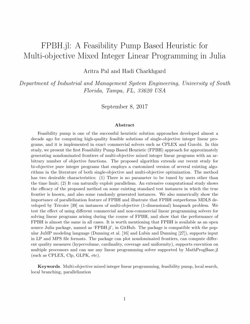
Figure 1: An illustration of the nondominated frontier of a MOMILP with p = 2

Overall, multi-objective optimization is concerned with finding a full representation of the non-dominated frontier. Specifically, min(x1,x2)∈X z(x1,x2) is defined to be precisely YN . An illustrationof the nondominated frontier of a MOMILP when p = 2 is shown in Figure 1 [5]. We observe thatsolving a MOMILP even when p = 2 is quite challenging since its nondominated frontier is not convexand it may contain some points, line segments, and even half-open (or open) line segments. It isevident that for p > 2, there may exist (hyper)plane segments in the nondominated frontier as well.

In light of the above, in this study, we develop a heuristic approach, i.e., FPBH, for approximatelyrepresenting the nondominated frontier of a MOMILP. FPBH simply approximates the nondominatedfrontier of a MOMILP by generating a finite set of feasible points. Since our algorithm is a heuristicmethod, there is no guarantee that the set of points generated by the method to be a subset of theexact nondominated points of the problem. However, the goal is that the set to be a high-qualityapproximation for the exact nondominated frontier in practice. Next, we introduce concepts andnotation that will facilitate the presentation and discussion of the proposed approach.

In FPBH, we often deal with a finite subset of feasible solutions, S ⊆ X , of which we would like toremove dominated solutions (those that are dominated by other feasible solutions of S). We denotethis operation by Pareto(S), and it simply returns the following set,

{(x1,x2) ∈ S : @(x′1,x′2) ∈ S with zi(x

′1,x

′2) ≤ zi(x1,x2) for i = 1, . . . , p ,z(x′1,x

′2) 6= z(x1,x2)}.

Note that in this operation, we make sure that the created set is minimal in a sense that if there aremultiple solutions with the same objective values then only one of them can be in the set. Let S ⊆ Xbe a finite subset of feasible solutions. Obviously, ∪(x1,x2)∈S{z(x1,x2) + Rp

≥} is the set of all pointsof the criterion space dominated by solutions in set S (of course the only exceptions are the points inset ∪(x1,x2)∈S{z(x1,x2)}). For example, suppose that S = {(x1

1,x12), (x2

1,x22)} and let y1 := z(x1

1,x12)

and y2 := z(x21,x

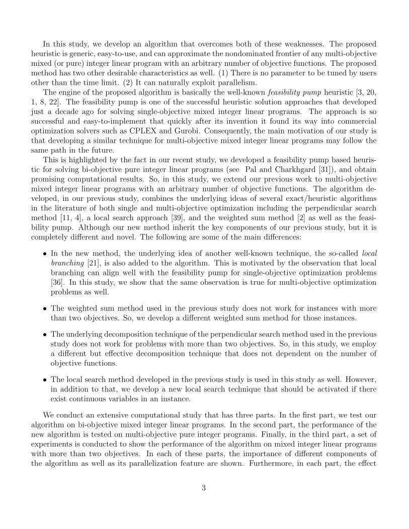
22). An illustration of the feasible points y1 and y2 and ∪(x1,x2)∈S{z(x1,x2) + Rp

≥}when p = 2 can be found in Figure 2a. Kirlik and Sayın [23] introduce a simple recursive algorithmfor finding the minimum set of points denoted by u1, . . . ,uK with the property that ∪Kk=1{uk − Rp

>}defines the set of all points in the criterion space that are not dominated by solutions in S. We callu1, . . . ,uK as the set of upper bound points, and use the operation Decompose(S) to compute them.An illustration of the upper bound points corresponding to y1 and y2, and also ∪Kk=1{uk −Rp

>} whenp = 2 can be found in Figure 2b. We next briefly explain how the recursive algorithm works.

5

y1

y2

+∞

+∞−∞ First objective value

Sec

on

dob

ject

ive

valu

e

(a) Dominated regions by y1 and y2

y1

y2

+∞

+∞−∞

u1

u2

u3

First objective value

Sec

ond

obje

ctiv

eva

lue

(b) Regions not dominated by y1 and y2

Figure 2: An illustration of the upper bound points when p = 2 and two feasible points y1 and y2 areknown

Let S = S ′ ∪ {(x1,x2)} and |S| = |S ′| + 1. Now, suppose that the minimum set of upper boundpoints corresponding to set S ′, denoted by u1, . . . ,uK , is known. As an aside, if S ′ = ∅ then weconsider +∞ := (+∞, . . . ,+∞) as the only upper bound point of the set S ′. Now, to compute theminimum set of upper bound points corresponding to set S, two steps should be taken:

• Step 1: For each k ∈ {1, . . . , K} with z(x1,x2) ≤ uk and z(x1,x2) 6= uk, we replace uk by pnew upper bound points denoted by uk,1, . . . ,uk,p. For each i = 1, . . . , p, we set uk,ii = zi(x1,x2)and uk,il = ukl for each l ∈ {1, . . . , p}\{i}.

• Step 2: Redundant elements of the set generated in Step 1 should be removed one by one inthis step. An upper bound uv is redundant if there exists another upper bound point uw suchthat uv ≤ uw.

Interested readers may refer to the study of Kirlik and Sayın [23] for further details about therecursive method for generating the upper bound points. It is worth mentioning that there are moreefficient but more complicated approach in order to compute the upper bound points (see for instance[17]). However, in this study, we use the simple approach explained above since it is easier to implement(and performs well in practice).

3 The framework of the proposed algorithm

The algorithm is a two-stage approach and it maintains a list of all x1 ∈ {0, 1}n1 that based onwhich the algorithm was not able to obtain a feasible solution. We call this list as Tabu and at thebeginning of the algorithm, this list is empty. The algorithm uses this list in all feasibility pumpoperations to avoid cycles. Since the size of the Tabu list becomes large during the course of the firststage, we make this list empty before starting the second stage to save the valuable computationaltime. The algorithm also maintains a set of feasible solutions, denoted by X , during the course of

6

Algorithm 1: The framework of the Algorithm

1 List.create(Tabu)

2 X ← 03 Time Limit Stage1← γ × Total T ime Limit4 Time Limit Stage2← (1− γ)× Total T ime Limit5 (X , Tabu)← Stage1 Algorithm

(X , Tabu, T ime Limit Stage1

)6 List.EraseElements(Tabu)

7 X ← Stage2 Algorithm(X , Tabu, T ime Limit Stage2)

8 return X

the algorithm. When the algorithm terminates this set will be reported as the set of approximateefficient solutions of the problem. In other words, when the algorithm terminates any two distinctsolutions (x1,x2), (x′1,x

′2) ∈ X do not dominate each other, i.e., there exist i, j ∈ {1, . . . , p} such that

zi(x1,x2) > zi(x′1,x

′2) and zj(x1,x2) < zj(x

′1,x

′2).

The algorithm takes two inputs including the total run time and the parameter γ ∈ (0, 1], whichis basically the ratio of the total run time that should be assigned to Stage 1 of the Algorithm.Consequently, (1 − γ) is the ratio of the total run time that should be assigned to Stage 2 of theAlgorithm. Since the second stage of the algorithm is only designed to further improve the results ofthe first stage, we have computationally observed that γ is better to be set to 2

3. Algorithm 1 shows

a precise description of the proposed method. We now make one final comment:

• Algorithms proposed in Stages 1 and 2 are similar and they are both feasibility pump basedheuristics. However, in Stage 1, the focus is more on the diversity of the points in the approximatenondominated frontier but, in Sage 2, the focus is more on the quantity of the points in theapproximate nondominated frontier. Consequently, the main technical difference between thesetwo stages is that, in Stage 1, the search for finding locally efficient solutions will continue inthe not yet dominated regions of the criterion space in each iteration. In order to do so, the setof upper bound points will be updated frequently during the course of Stage 1. However, in thesecond stage, this condition is relaxed with the hope of finding more locally efficient solutions.Moreover, a variation of the local branching heuristic (see for instance [21, 36]) is incorporatedin the second stage for the same purpose.

3.1 Stage 1

The heuristic algorithm (of Stage 1) is specifically designed for finding locally nondominated pointsfrom different parts of the criterion space. In other words, the focus of this stage is on the diversityof the points in the approximate nondominated frontier. The heuristic algorithm in this stage isinitialized by X , the Tabu list, and the time limit for stage 1. The algorithm maintains a queue ofupper bound points, denoted by Q. The queue will be initialized by the point +∞ = (+∞, . . . ,+∞).The algorithm terminates when the run time violates the imposed time limit or when the queue isempty. Next we explain the workings of the heuristic algorithm (of Stage 1) at any arbitrary iteration.

In each iteration, the algorithm pops out an element, i.e., an upper bound point, from thequeue, which is denoted by u. Note that when an element is popped out then that element does

7

+∞

+∞−∞

u

First objective value

Sec

on

dob

ject

ive

valu

e

(a) The search regioin defined by u

+∞

+∞−∞

u

First objective value

Sec

on

dob

ject

ive

valu

e

(b) The outcome of the feasibilitypump operation

+∞

+∞−∞

u

First objective value

Sec

on

dob

ject

ive

valu

e

(c) The outcome of the local searchoperation

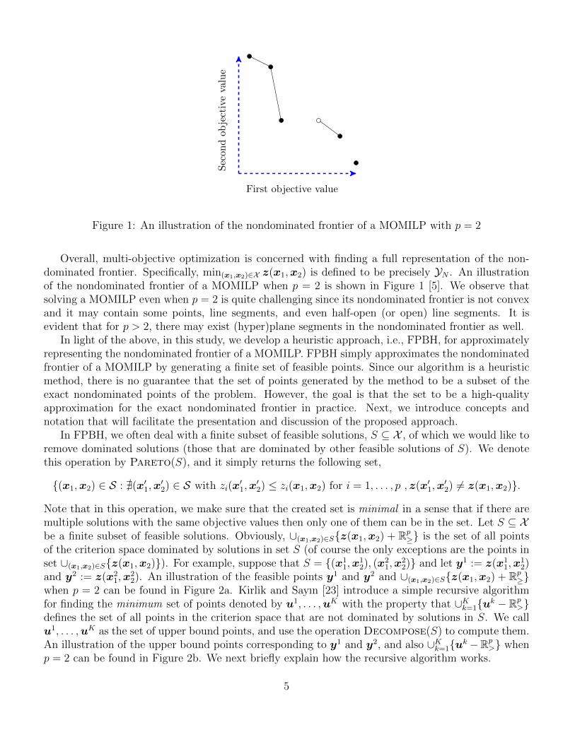
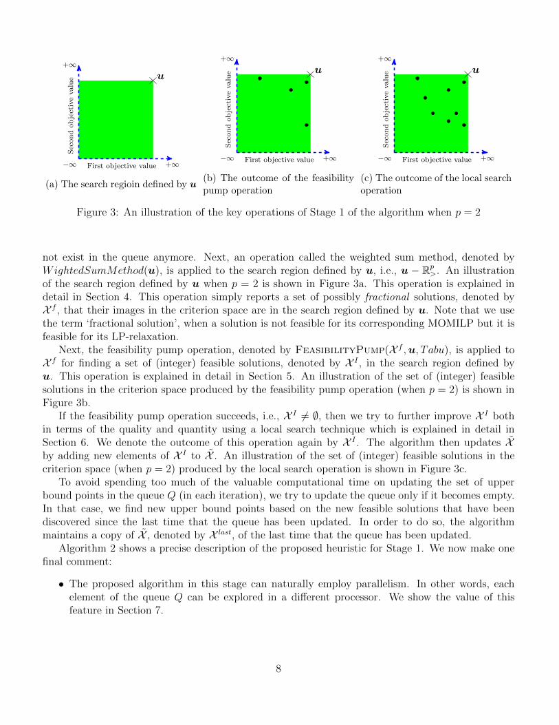
Figure 3: An illustration of the key operations of Stage 1 of the algorithm when p = 2

not exist in the queue anymore. Next, an operation called the weighted sum method, denoted byWightedSumMethod(u), is applied to the search region defined by u, i.e., u − Rp

>. An illustrationof the search region defined by u when p = 2 is shown in Figure 3a. This operation is explained indetail in Section 4. This operation simply reports a set of possibly fractional solutions, denoted byX f , that their images in the criterion space are in the search region defined by u. Note that we usethe term ‘fractional solution’, when a solution is not feasible for its corresponding MOMILP but it isfeasible for its LP-relaxation.

Next, the feasibility pump operation, denoted by FeasibilityPump(X f ,u, Tabu), is applied toX f for finding a set of (integer) feasible solutions, denoted by X I , in the search region defined byu. This operation is explained in detail in Section 5. An illustration of the set of (integer) feasiblesolutions in the criterion space produced by the feasibility pump operation (when p = 2) is shown inFigure 3b.

If the feasibility pump operation succeeds, i.e., X I 6= ∅, then we try to further improve X I bothin terms of the quality and quantity using a local search technique which is explained in detail inSection 6. We denote the outcome of this operation again by X I . The algorithm then updates Xby adding new elements of X I to X . An illustration of the set of (integer) feasible solutions in thecriterion space (when p = 2) produced by the local search operation is shown in Figure 3c.

To avoid spending too much of the valuable computational time on updating the set of upperbound points in the queue Q (in each iteration), we try to update the queue only if it becomes empty.In that case, we find new upper bound points based on the new feasible solutions that have beendiscovered since the last time that the queue has been updated. In order to do so, the algorithmmaintains a copy of X , denoted by X last, of the last time that the queue has been updated.

Algorithm 2 shows a precise description of the proposed heuristic for Stage 1. We now make onefinal comment:

• The proposed algorithm in this stage can naturally employ parallelism. In other words, eachelement of the queue Q can be explored in a different processor. We show the value of thisfeature in Section 7.

8

Algorithm 2: Stage1 Algorithm(X , Tabu, T ime Limit Stage1

)1 Queue.create(Q);2 Queue.add

(Q,+∞

)3 X last ← ∅4 while time ≤ Time Limit Stage1 & not Queue.empty(Q) do5 Queue.pop(Q,u)

6 X f ←WeightedSumMethod(u)

7 (X I , Tabu)← FeasibilityPump(X f ,u, Tabu)8 if X I 6= ∅ then9 X I ← LocalSearch(X I ,u)

10 X ← X ∪ X I

11 if Queue.empty(Q) then

12 U ← Decompose(X \X last)13 foreach u′ ∈ U do14 Queue.add

(Q,u′

)15 X last ← X

16 return(Pareto(X ), Tabu

)3.2 Stage 2

Two key differences of this stage with the previous one are that:

• Instead of using the weighted sum method for generating a set of fractional solutions, a variationof the local branching approach (see for instance [21, 36]) is used.

• The upper bound points are not computed in this stage and so the search is not limited to theregions defined by these points.

Overall, these two key differences help us find more feasible solutions. So, the focus of Stage 2 is onthe quantity of the points in the approximate nondominated frontier. Before presenting the details ofthe algorithm, we explain the local branching operation which is denoted by

LocalBranching(S, UpperLimit, Step),

where X new ⊆ X and UpperLimit, Step ∈ Z≥ are its inputs. The output of this operation is a set ofpossibly fractional solutions denoted by X f . In this operation, for each (x′1,x

′2) ∈ X new, the following

optimization problem should be solved:

(x∗1,x∗2) = arg min

{ p∑i=1

zi(x1,x2) : (x1,x2) ∈ LP (X ),

UpperLimit− Step ≤n1∑

j=1: x′1,j=0

x1,j +

n1∑j=1: x′1,j=1

(1− x1,j) ≤ UpperLimit}.

9

It is evident that this optimization problem seeks to produce a (possibly fractional) solution in the LP-relaxation of the problem such that the difference between its values of the integer decision variablesfrom those of solution (x′1,x

′2) to be within a specific neighborhood. The objective function of the

optimization problem ensures that the new (possibly fractional) solution to be close to the exactnondominated frontier of the corresponding MOMILP. If (x∗1,x

∗2) exists and it is not already in X f

then we add it to X f .We now explain the heuristic algorithm (of Stage 2) in detail. The algorithm is initialized by

X , the Tabu list, and the time limit for Stage 2. The initial values of UpperBound and Step areset to 2 and 1, respectively. It is worth mentioning that we could initialize UpperBound = 1 andStep = 0, but this case will be naturally explored in the feasibility pump operation (and so we havetried to remove any redundant calculation). The algorithm terminates when the run time violatesthe imposed time limit or UpperLimit > n1. In each iteration, the algorithm makes a copy of Xand denote it by X new. Also, the algorithm measures the cardinality of X at the beginning of eachiteration and denote it by InitialCardinality. It then explores and updates the set X new by using aset of operations until it becomes empty. Afterwards, it updates the values of Step and UpperLimit(based on InitialCardinality) before starting the next iteration.

Algorithm 3: Stage2 Algorithm(X , Tabu, T ime Limit Stage2)

1 UpperLimit← 22 Step← 13 while UpperLimit ≤ n1 & time ≤ Time Limit Stage2 do

4 X new ← X5 InitialCardinality ← |X |6 SearchDone← False7 while SearchDone = False do8 X f ← LocalBranching(X new, UpperLimit, Step)9 (X I , Tabu)← FeasibilityPump(X f ,+∞, Tabu)

10 if X I 6= ∅ then11 X I ← LocalSearch(X I ,+∞)

12 X new ← NewSolutions(X I , X )

13 X ← X ∪ X I

14 else15 X new ← ∅16 if X new = ∅ then17 SearchDone← True

18 if |X | − InitialCardinality ≤ UpperLimit then19 Step← Step+ 1

20 UpperLimit← UpperLimit+ Step+ 1

21 return Pareto(X )

In particular, to explore and update the set X new in each iteration, the following steps are con-ducted. The algorithm first calls LocalBranching(X new, UpperLimit, Step) to compute a set ofpossibly fractional solutions X f . Next, it calls FeasibilityPump(X f ,+∞, Tabu) for finding a set

10

of (integer) feasible solutions, i.e., X I . If the feasibility pump operation fails, i.e., X I = ∅, then thealgorithm sets X new = ∅ since it was not able to find new feasible solutions. Otherwise, i.e., X I 6= ∅,the algorithm attempts to further improve X I both in terms of the quality and quantity by calling thelocal search operation. We denote the outcome of this operation again by X I . The algorithm then setsX new to the solutions of X I in which their corresponding images in the criterion space are differentfrom those in the set X . This operation is denoted by NewSolutions(X I , X ). The algorithm thenupdates X by adding new elements of X I to X .

If X new 6= ∅ then all the steps (mentioned above) will be repeated for the updated X new. Otherwise,the values of Step and UpperLimit should be increased. In order to do so, we have employed a simpletechnique that ensures that if the the number of the new solutions produced in each iteration is notlarge enough then the value of UpperLimit increases with a higher speed. In order to do so, we firstcheck whether

|X | − InitialCardinality ≤ UpperLimit.

If this is the case then we increase the Step by one. Finally, we increase the size of UpperLimit byStep+1. Algorithm 3 shows a precise description of the proposed heuristic for Stage 2. We now makeone final comment:

• The proposed algorithm in this phase can also employ parallelism. In our implementation, if wehave p different processors, we simply split X new into p subsets with (almost) equal size. Wethen assign each subset to a different processor and apply the local branching, feasibility pumpand local search operations on that subset. We show the value of this feature in Section 7.

yT

yB

First objective value

Sec

ond

obje

ctiv

eva

lue

(a) The endpoints of the nondominated frontier

yT

yBy∗

First objective value

Sec

ond

obje

ctiv

eva

lue

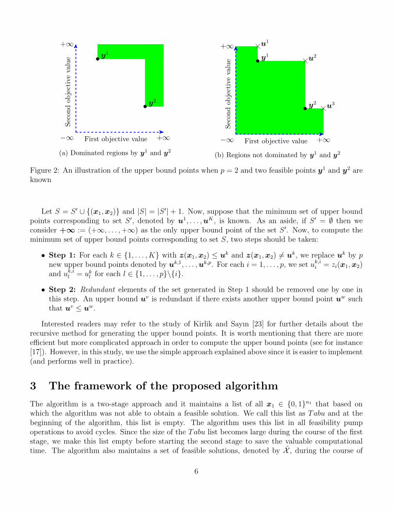
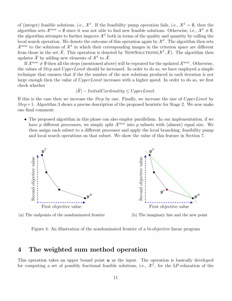
(b) The imaginary line and the new point

Figure 4: An illustration of the nondominated frontier of a bi-objective linear program

4 The weighted sum method operation

This operation takes an upper bound point u as the input. The operation is basically developedfor computing a set of possibly fractional feasible solutions, i.e., X f , for the LP-relaxation of the

11

problem that their images in the criterion space lie within the search region defined dy u, i.e., u−Rp>.

Specifically, the operation generates and return some of the efficient solutions of the following problem:

min{z1(x1,x2), . . . , zp(x1,x2) : (x1,x2) ∈ LP (X ), zi(x1,x2) < ui for all i ∈ {1, . . . , p}

}. (2)

It is worth mentioning that Problem (2) is basically a multi-objective linear program and it iswell-known that the nondominated frontier of such a problem is connected. An illustration of thenondominated frontier of a multi-objective linear program with p = 2 can be found in Figure 4a.Overall, the main goal of the weighted sum method operation is that the generated efficient solutions(mainly) correspond to the extreme nondominated points of Problem (2), i.e., circles in Figure 4a.Based on the theory of multi-objective linear programming (see for instance [18]), for any efficientsolution (x∗1,x

∗2) of Problem (2), there exists a weight vector λ ∈ Rp

> such that:

(x∗1,x∗2) ∈ arg min

{ p∑i=1

λizi(x1,x2) : (x1,x2) ∈ LP (X ), zi(x1,x2) < ui for all i ∈ {1, . . . , p}}. (3)

We denote this operation by ArgWeightedMin(λ,u). So, in order to generate X f , we onlyneed to update λ and solve Problem (3) in each iteration. It is worth mentioning that we havecomputationally observed that the performance of FPBH improves, if we terminate the weighted summethod operation as soon as the cardinality of X f does not satisfy the following condition:

|X f | ≤ CardinalityBound := dmin{10

pdlogp he,

100

p}e,

where h := max{m,n1 + n2}. Note that based on our discussion in Section 2, m is the number ofconstraints and n1 +n2 is the number of variables. So, this observation is taken into account in FPBH.

4.1 Instances with two objectives

It is well-known (see for instance [2]) that when p = 2, updating λ can be done efficiently if the topand bottom endpoints of the nondominated frontier are known. So, when p = 2, we first find theendpoints of the nondominated frontier by using a lexicographical technique. For example, the topendpoint, denoted by yT := z(xT1 ,x

T2 ), can be computed by first solving,

(x1, x2) ∈ arg min{z1(x1,x2) : (x1,x2) ∈ LP (X ), zi(x1,x2) < ui for all i ∈ {1, 2}

},

and if it is feasible, it needs to be followed by solving,

(xT1 ,xT2 ) ∈ arg min

{z2(x1,x2) : z1(x1,x2) ≤ z1(x1, x2),

(x1,x2) ∈ LP (X ), zi(x1,x2) < ui for all i ∈ {1, 2}}.

We denote this operation by ArgLexMin(1, 2,u). By computing (xT1 ,xT2 ), the first potential

fractional solution has been generated and so it should be added to X f . The bottom endpoint,denoted by yB := z(xB1 ,x

B2 ), can be obtained similarly and so (xB1 ,x

B2 ) should also be added to X f

(if yT 6= yB). We denote the operation of finding a solution corresponding to the bottom endpoint byArgLexMin(2, 1,u). These two points form the first pair of points (yT ,yB) and they will be addedto a queue of pairs of points (if yT 6= yB and |X f | ≤ CardinalityBound).

12

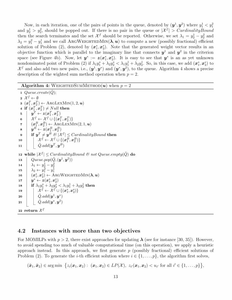
Now, in each iteration, one of the pairs of points in the queue, denoted by (y1,y2) where y11 < y2

1

and y12 > y2

2, should be popped out. If there is no pair in the queue or |X f | > CardinalityBoundthen the search terminates and the set X f should be reported. Otherwise, we set λ1 = y1

2 − y22 and

λ2 = y21 − y1

1 and we call ArgWeightedMin(λ,u) to compute a new (possibly fractional) efficientsolution of Problem (2), denoted by (x∗1,x

∗2). Note that the generated weight vector results in an

objective function which is parallel to the imaginary line that connects y1 and y2 in the criterionspace (see Figure 4b). Now, let y∗ := z(x∗1,x

∗2). It is easy to see that y∗ is an as yet unknown

nondominated point of Problem (2) if λ1y∗1 + λ2y

∗2 < λ1y

11 + λ2y

12. So, in this case, we add (x∗1,x

∗2) to

X f and also add two new pairs, i.e., (y1,y∗) and (y∗,y2), to the queue. Algorithm 4 shows a precisedescription of the wighted sum method operation when p = 2.

Algorithm 4: WeightedSumMethod(u) when p = 2

1 Queue.create(Q);

2 X f ← ∅3 (xT1 ,x

T2 )← ArgLexMin(1, 2,u)

4 if (xT1 ,xT2 ) 6= Null then

5 yT ← z(xT1 ,xT2 )

6 X f ← X f ∪ {(xT1 ,xT2 )}7 (xB1 ,x

B2 )← ArgLexMin(2, 1,u)

8 yB ← z(xB1 ,xB2 )

9 if yT 6= yB & |X f | ≤ CardinalityBound then10 X f ← X f ∪ {(xB1 ,xB2 )}11 Q.add(yT ,yB)

12 while |X f | ≤ CardinalityBound & not Queue.empty(Q) do

13 Queue.pop(Q, (y1,y2))14 λ1 ← y1

2 − y22

15 λ2 ← y21 − y1

1

16 (x∗1,x∗2)← ArgWeightedMin(λ,u)

17 y∗ ← z(x∗1,x∗2)

18 if λ1y∗1 + λ2y

∗2 < λ1y

11 + λ2y

12 then

19 X f ← X f ∪ {(x∗1,x∗2)}20 Q.add(y1,y∗)

21 Q.add(y∗,y2)

22 return X f

4.2 Instances with more than two objectives

For MOMILPs with p > 2, there exist approaches for updating λ (see for instance [30, 35]). However,to avoid spending too much of valuable computational time (on this operation), we apply a heuristicapproach instead. In this approach, we first generate p (possibly fractional) efficient solutions ofProblem (2). To generate the i-th efficient solution where i ∈ {1, . . . , p}, the algorithm first solves,

(x1, x2) ∈ arg min{zi(x1,x2) : (x1,x2) ∈ LP (X ), zi′(x1,x2) < ui′ for all i′ ∈ {1, . . . , p}

},

13

and if it is feasible, it needs to be followed by solving,

(x∗1,x∗2) ∈ arg min

{ p∑i′=1

zi′(x1,x2) : zi(x1,x2) ≤ zi(x1, x2),

(x1,x2) ∈ LP (X ), zi′(x1,x2) < ui′ for all i′ ∈ {1, . . . , p}}.

We denote this operation by TwoPhase(i,u) where i ∈ {1, . . . , p} and its corresponding efficientsolution (x∗1,x

∗2) should be added to X f [23]. The remaining necessary efficient solutions are generated

randomly by creating a set of weight vectors denoted by Λ. Components of each weight vector λ ∈ Λare generated randomly from the standard normal distribution, denoted by RandNormal(0, 1), butwe use the absolute value of the generated random numbers. We also normalize the components ofeach weight vector to assure that the summation of its components is equal to one.

Algorithm 5: WeightedSumMethod(u) when p > 2

1 X f ← ∅2 foreach i ∈ {1, . . . , p} do3 if CardinalityBound > 0 then4 (x∗1,x

∗2)← TwoPhase(i,u)

5 X f ← X f ∪ {(x∗1,x∗2)}6 CardinalityBound← CardinalityBound− 1

7 Λ← ∅8 while |Λ| ≤ CardinalityBound do9 foreach i ∈ {1, . . . , p} do

10 λi ← |RandNormal(0, 1)|11 foreach i ∈ {1, . . . , p} do12 λi ← λi∑p

j=1 λj

13 Λ← Λ ∪ {λ}14 foreach λ ∈ Λ do15 (x∗1,x

∗2)← ArgWeightedMin(λ,u)

16 X f ← X f ∪ {(x∗1,x∗2)}17 X f ← Distinct(X f )

18 return X f

Next, for each λ ∈ Λ, we call ArgWeightedMin(λ,u) to compute a new (possibly fractional)efficient solution for Problem (2), denoted by (x∗1,x

∗2), and add it to X f . Algorithm 5 shows a precise

description of the weighted sum method operation when p > 2. During the course of the algorithm,the number of efficient solutions generated by the algorithm is no more than CardinalityBound.Moreover, the algorithm removes equivalent solutions, meaning if there are several efficient solutionswith the same image in the criterion space, only one of them will be reported. This operation isdenoted by Distinct(X f ) in Algorithm 5.

14

5 The feasibility pump operation

Our proposed feasibility pump approach is similar to the feasibility pump approach used for single-objective integer linear programs. The single-objective version of the feasibility pump works on a pairof solutions (xf1 ,x

f2) and (xI1,x

I2). The first one is feasible for the LP-relaxation of the problem, and so

it may be fractional. However, the latter is integer but it is not necessarily feasible for Problem (1), i.e.,geometrically it may lie outside the polyhedron corresponding to the LP-relaxation of the problem.The feasibility pump iteratively updates (xf1 ,x

f2) and (xI1,x

I2), and in each iteration, the hope is

to further reduce the distance between them. Consequently, ultimately, we can hope to obtain an(integer) feasible solution.

In light of the above, we now present our proposed feasibility pump operation. This operationtakes a set of possibly fractional solutions X f , an upper bound point u, and the Tabu list as inputs,and returns the updated Tabu list, and a set of (integer) feasible solutions, X I . At the beginning, weset X I = ∅. Also, at the end, we call Distinct(X I) to remove the equivalent solutions of X I beforereturning it.

The feasibility pump operation attempts to construct some integer feasible solutions in the searchregion defined by u, i.e., u − Rp

>, based on each (x1, x2) ∈ X f . By construction of FPBH, if x1 ∈{0, 1}n1 then we must have that (x1, x2) ∈ X , zi(x1, x2) < ui for all i = 1, . . . , p. So, in that case,(x1, x2) is an integer feasible solution in the search region defined by u, and so (x1, x2) should beadded to X I .

Let e be the base of the natural logarithm. If x1 /∈ {0, 1}n1 then the algorithm attempts toconstruct at most |Θ| = p+ 1 integer feasible solutions based on (x1, x2) where,

Θ := {0, e1∑pj=1 e

j, . . . ,

ep∑pj=1 e

j},

is a set of weights to modify the distance function in the feasibility pump operation (at the end ofthis section, the details of the distance function are explained). Specifically, for each θ ∈ Θ, we setthe maximum number of attempts for constructing an integer feasible solution based on (x1, x2) to beequal to the number of variables with fractional values in x1, denoted by FractionalDegree(x1).For a given (x1, x2) and θ, before starting the set of attempts to generate an integer feasible solution,we make a copy of (x1, x2) and denote it by (xf1 ,x

f2). The set of attempts will be conducted on

(xf1 ,xf2). As soon as an integer feasible solution is found, the algorithm will terminate its search for

constructing integer feasible solutions based on (x1, x2) and θ. Next, we explain the workings of thealgorithm during each attempt for constructing an integer feasible solution based on (x1, x2) and θ.Note that in the remaining, whenever we say that ‘the search will terminate’, we mean that the searchfor constructing an integer feasible solution based on (x1, x2) and θ will terminate.

During each attempt, the algorithm first rounds each component of xf1 . This operation is de-noted by Round(xf1). We define (xI1,x

I2) := (Round(x1),xf2). Next, the algorithm checks whether

(xI1,xI2) ∈ X and zi(x

I1,x

I2) < ui for all i ∈ {1, . . . , p}. If that is the case then the algorithm has

found an integer feasible solution in the search region defined by u. So, the search will terminateafter adding (xI1,x

I2) to X I . So, in the remaining we assume that the search does not terminate after

computing (xI1,xI2).

In this case, the algorithm first checks whether xI1 is in the Tabu list. If it is then the algorithm triesto modify xI1 by using a flipping operation that flips some components of xI1, i.e., if a component has

15

Algorithm 6: FeasibilityPump(X f ,u, Tabu)

1 X I ← ∅2 foreach (x1, x2) ∈ X f do3 if x1 ∈ {0, 1}n1 then4 X I ← X I ∪ {(x1, x2)}5 else6 Max Iteration← FractionalDegree(x1)7 foreach θ ∈ Θ do8 SearchDone← False9 t← 1

10 (xf1 ,xf2)← (x1, x2)

11 while SearchDone = False & t ≤Max Iteration do

12 (xI1,xI2)←

(Round(xf1),xf2

)13 if (xI1,x

I2) ∈ X & z1(xI1,x

I2) < u1 & . . . & zp(x

I1,x

I2) < up then

14 X I ← X I ∪ {(xI1,xI2)}15 SearchDone← True

16 else17 if xI1 ∈ Tabu then

18 xI1 ← FlippingOperation(xf1 ,xI1, Tabu)

19 if xI1 = Null then20 SearchDone← True

21 else22 if (xI1,x

I2) ∈ X & z1(xI1,x

I2) < u1 & . . . & zp(x

I1,x

I2) < up then

23 X I ← X I ∪ {(xI1,xI2)}24 SearchDone← True

25 if SearchDone = False then26 Tabu.add(xI1)

27 (xf1 ,xf2)← FeasibilitySearch(xI1,u, θ)

28 t← t+ 1

29 X I ← Distinct(X I)30 return (X I , Tabu)

16

the value of zero then we may change it to one, and the other way around. We explain the details of thisoperation in Section 5.1. We denote the flipping operation by FlippingOperation(Tabu,xf1 ,x

I1),

and it returns an updated xI1. If xI1 = Null then the flipping operation has failed and in this case, thealgorithm will terminate its search. However, if xI1 6= Null then there is a possibility that (xI1,x

I2) to

be an integer feasible solution. So, we again check whether (xI1,xI2) ∈ X and zi(x

I1,x

I2) < ui for all

i ∈ {1, . . . , p}. If that is the case then we have found an integer feasible solution. So, again the searchwill terminate after adding (xI1,x

I2) to X I .

Finally, regardless of whether xI1 is in the Tabu list or not, if the search has not terminated yet,the algorithm takes two further steps:

• It adds xI1 to the Tabu list; and

• It updates (xf1 ,xf2) using xI1 by solving the following optimization problem,

(xf1 ,xf2) = arg min

{(1− θ)∆(xI1) + θ

∑pi=1 zi(x1,x2)√∑n1

j=1(∑p

i=1 cij)2 +

∑n2

j=1(∑p

i=1 dij)2

:

(x1,x2) ∈ LP (X ),

zi(x1,x2) < ui for all i ∈ {1, . . . , p}},

where

∆(xI1) :=

n1∑j=1: xI1,j=0

x1,j +

n1∑j=1: xI1,j=1

(1− x1,j).

The goal of this optimization problem is to find a (possibly fractional) solution, which is closerto (xI1,x

I2). We denote this optimization problem by FeasibilitySearch(xI1 u, θ), and its

objective function is the distance function that we have used in our study. The first part of thedistance function tries to minimize the distance between the new xf1 and xI1, but the second partis only for modifying the distance function based on the normalized value of

∑pi=1 zi(x1,x2).

Note that the distance function that we have used is similar to the typical distance functionused in the feasibility pump heuristic for single-objective optimization problems [20, 22]. Onlythe second part of the distance function is modified here since we are dealing with multipleobjectives. Note too that the set Θ introduced at the beginning of this section performs the bestfor our test instances. In practice, we realized that the existence of a linear relationship betweenelements of Θ does not help. So, we generated Θ such that there is a non-linear relationshipbetween its elements.

Algorithm 6 shows a precise description of the proposed feasibility pump operation. We now makeone final comment:

• In practice, we have observed that if it turns out that xI1 = ∅ at Line 19 of Algorithm 6 then itis unlikely to find any feasible solution for the remaining elements of Θ. So, in this case, it isbetter to directly return to Line 2 of the code for selecting a new element of X f .

17

5.1 The flipping operation

The flipping operation takes the Tabu list, xf1 (which is fractional), and the integer solution xI1 asinputs. Obviously, by construction, xI1 is in the Tabu list. So, this operation attempts to flip thecomponents of xI1 with the hope that the outcome to not be an element of the Tabu list. As soon asone is found, the flipping operation terminates, and the updated xI1 will be returned.

At the beginning of the operation, we construct two vectors of variables denoted by x∗1 and xI1.Specifically, we set x∗1 = null at the beginning of the operation, but at the end, this vector containsthe updated value of xI1 (if we find any) that should be reported. The vector xI1 is a copy of (initialvalue) of xI1 and all necessary flips will be conducted on xI1.

Overall, the flipping operation, contains two parts including a deterministic procedure and astochastic procedure. The stochastic procedure will be activated only if the deterministic fails toupdate xI1, i.e., if x∗1 is still null after the deterministic procedure. It is worth mentioning that wehave computationally observed that this order performs better than first doing the stochastic proce-dure and then deterministic procedure.

Before explaining these two procedures, a new operation denoted by SortIndex(xf1 ,xI1) is intro-

duced. This operation simply sorts the set {j ∈ {1, . . . , n} : |xf1,j − xI1,j| 6= 0} based on the value of

|xf1,j − xI1,j| from large to small. Note that, by construction, if xf1,j is not fractional then xI1,j = xf1,j(because xI1,j is the rounded value of xf1,j). This implies that this operation sorts the index set of

fractional components of xf1 . We denote the result of this operation by {s1, . . . , sM} where

|xf1,sk− xI1,sk | ≥ |x

f1,sk+1 − xI1,sk+1|

for each k = 1, . . . ,M − 1.The deterministic procedure attempts at most M times to update xI1. At the beginning, we set

xI1 = xI1. During attempt j ≤ M , we flip the component xI1,sj . This implies that if xI1,sj = 1 then

we make it equal to zero, and the other way around. We denote this operation by Flip(xI1, sj). If

the result is not in the Tabu list then the algorithm terminates, and we set x∗1 to xI1. Otherwise, (ifpossible) a new attempt will be started.

The stochastic procedure also attempts at most M times to construct an integer solution. Ateach attempt, we first set xI1 = xI1 and then we randomly select an integer number from the interval[dM

2e,M − 1]. This operation is denoted by RandBetween(dM

2e,M − 1), and its result is denoted

by Num. We then randomly generate a set denoted by R such that R ⊆ {1, . . . ,M} and |R| = Num.The operation is denoted by RandomlyChoose(Num, {1, . . . ,M}). We then flip the componentxI1,sr for each r ∈ R. If the result is not in the Tabu list then the algorithm terminates, and we set x∗1to xI1. Otherwise, (if possible) a new attempt will be started.

Algorithm 7 shows a precise description of FlippingOperation(xf1 ,xI1, Tabu).

6 The local search operation

The local search operation (that we have developed) has two stages. The operation takes X I (whichis a subset of the feasible solutions of Problem (1)) and u as inputs, and reports an updated X I . Thefirst stage will be only activated when n1 > 0 and n2 > 0, i.e., the instance is a mixed integer linearprogram. The second stage will be immediately called after the first stage regardless of whether the

18

instance is a pure integer program or mixed integer program. A precise description of the local searchoperation can be found in Algorithm 8.

Algorithm 7: FlippingOperation(xf1 ,xI1, Tabu)

1 {s1, . . . , sM} ← SortIndex(xf1 ,xI1)

2 x∗1 ← Null

3 xI1 ← xI14 j ← 15 while j ≤M and x∗1 = Null do

6 xI1 ← Flip(xI1, sj)

7 if xI1 /∈ Tabu then

8 x∗1 ← xI1

9 else10 j ← j + 1

11 j ← 112 while j ≤M and x∗1 = Null do

13 xI1 ← xI114 Num← RandBetween(dM2 e,M − 1)15 R← RandomlyChoose(Num, {1, . . . ,M})16 foreach r ∈ R do

17 xI1 ← Flip(xI1, sr)

18 if xI1 /∈ Tabu then

19 x∗1 ← xI1

20 else21 j ← j + 1

22 xI1 ← x∗123 return xI1

6.1 The local search - Stage 1

The operation developed for Stage 1 takes X I (which is a subset of the feasible solutions of Problem (1))and u as inputs, and reports an updated X I . The key idea behind this operation comes from thefact that any (x1,x2) ∈ X I is an integer feasible solution for Problem (1). So, if we set the integerdecision variables of the corresponding MOMILP to x1, a multi-objective linear program will beconstructed. Obviously, all feasible solutions of such a multi-objective linear program are also feasiblefor the corresponding MOMILP. Consequently, we can attempt to enumerate some of the extremenondominated points of such a multi-objective linear program since they may be part of the truenondominated frontier of the corresponding MOMILP.

In light of the above, in this operation, we first make a copy of X I and denote it by X . We start byfirst removing redundant elements of X . This implies that for any (x1, x2), (x′1, x

′2) ∈ X with x1 = x′1

only one of them should remain in the set. We denote this operation by Unique(X ) and its outcome

19

Algorithm 8: LocalSearch(X I ,u)

1 if n1 > 0 and n2 > 0 then2 X I ← LocalSearch-Stage1(X I ,u)

3 X I ← LocalSearch-Stage2(X I ,u)4 return X I

is denoted by X again.We also denote the set of new feasible solutions by X ∗ which is empty at the beginning of the opera-

tion. For each (x1, x2) ∈ X , we call an operation entitled ModifiedWeightedSumMethod(x1,u)which is precisely the weighted sum operation that we explained in Section 4 with two small differ-ences. Basically, the first difference is that the following constraints should be added to any modelthat should be solved in the weighted sum operation:

x1,j = x1,j ∀j ∈ {1, . . . , n1}.

The second difference is that to avoid spending too much of valuable computational time on themodified wighted sum method, we set

CardinalityBound = dmin{10

pdlogp he,

100

p}

|Unique(X I)|e.

The set of solutions found by ModifiedWeightedSumMethod(x1,u) must be feasible for Prob-lem (1) (and lie within the search region defined by u), and so they will be added to X ∗. Finally, wecall Distinct(X I ∪X ∗) to compute the distinct elements of X I ∪X ∗ and report them as the updatedX I .

A precise description of Stage 1 of the local search operation can be found in Algorithm 9.

Algorithm 9: LocalSearch-Stage1(X I ,u)

1 X ← X I

2 X ← Unique(X )3 X ∗ ← ∅4 foreach (x1, x2) ∈ X do5 X ∗ ← X ∗ ∪ModifiedWeightedSumMethod(x1,u)

6 X I ← Distinct(X I ∪ X ∗)7 return X I

6.2 The local search - Stage 2

The operation developed for Stage 2 also takes X I (which is a subset of the feasible solutions ofProblem (1)) and u as inputs, and reports an updated X I after calling Pareto(X I). In this operation,

the algorithm first makes a copy of X I and denote it by X . For each (x1, x2) ∈ X , the algorithm tries

20

to generate at most n1 new (integer) feasible solutions for Problem (1) that lie within the search region

defined by u, and add them to X l. More precisely, for each (x1, x2) ∈ X and each j ∈ {1, . . . , n1}, thealgorithm first makes a copy of (x1, x2), denoted by (xnew1 ,xnew2 ). It then explores the consequenceof flipping component xnew1,j . Obviously, if xnew1,j = 1 and c1,j > 0 or c2,j > 0 or . . . or cp,j > 0 thenthe flipping can improve the value of at least one objective function. So, in this case, the algorithmchecks whether the new solution after flipping is feasible for Problem (1) and lies within the searchregion defined by u, and if that is the case then the algorithm adds it to X I . Similarly, if xnew1,j = 0and either c1,j < 0 or c2,j < 0 or . . . or cp,j < 0, then the flipping can improve the value of at leastone objective function. So, again, in this case, it checks whether the new solution after flipping isfeasible for Problem (1) and lies within the search region defined by u, and if that is the case thenthe algorithm adds it to X I .

Algorithm 10: LocalSearch-Stage2(X I ,u)

1 X ← X I

2 foreach (x1, x2) ∈ X do3 foreach j ∈ {1, . . . , n1} do4 (xnew1 ,xnew2 )← (x1, x2)5 if x1,j = 1 and (c1,j > 0 or . . . or cp,j > 0) then6 xnew1,j ← 0

7 if (xnew1 ,xnew2 ) ∈ X and z1(xnew1 ,xnew2 ) < u1 and . . . and zp(xnew1 ,xnew2 ) < up then

8 X I ← X I ∪ {(xnew1 ,xnew2 )}

9 else10 if x1,j = 0 and (c1,j < 0 or . . . or cp,j < 0) then11 xnew1,j ← 1

12 if (xnew1 ,xnew2 ) ∈ X and z1(xnew1 ,xnew2 ) < u1 and . . . and zp(xnew1 ,xnew2 ) < up then

13 X I ← X I ∪ {(xnew1 ,xnew2 )}

14 X I ← Pareto(X I)15 return X I

Algorithm 10 shows a precise description of LocalSearch-Stage2(X I ,u). We note that if thereare too many equality constraints in Problem (1), the second stage of the local search operation mostlikely will fail to generate any new integer feasible solution. So, we only activate this stage if at least5% of constraints are inequalities.

7 Computational Study

To evaluate the performance of the proposed method, we conduct a comprehensive computationalstudy. We use the Julia programming language to implement the proposed approach, and employCPLEX 12.7 as the single-objective linear programming solver. All computational experiments arecarried out on a Dell PowerEdge R630 with two Intel Xeon E5-2650 2.2 GHz 12-Core Processors(30MB), 128GB RAM, operating on a RedHat Enterprise Linux 6.8 operating system. It is worth

21

mentioning that FPBH and the instances are available as open source Julia packages at https:

//goo.gl/fwgHjO and https://goo.gl/mevqbk, respectively. The Julia package is compatible withthe popular JuMP modeling language (Dunning et al. [16], Lubin and Dunning [27]), supports inputin LP and MPS file formats, can plot nondominated frontiers, can compute different quality measures(hypervolume, cardinality, coverage and uniformity), supports execution on multiple processors andcan use any linear programming solver supported by MathProgBase.jl (such as CPLEX, Clp, GLPK,etc). An efficient implementation of FPBH specifically using CPLEX.jl for CPLEX is also availableas an open source Julia package at https://goo.gl/Yne4eU. Note that the default version used inthis paper is the efficient implementation of FPBH using CPLEX.jl, since during the course of thealgorithm, it does not have to rebuild the linear programming models (used in FPBH) repetitively.All experimental results and the nondominated frontiers of all instances computed in this study areavailable at https://goo.gl/xYxtiq and https://goo.gl/P4rPrB, respectively.

In total, 351 instances are used in this study. Some necessary information about these instancessuch as the size and some studies that have used them can be found in Table 1 where ‘#Const’ and‘#Ins’ are the number of constraints and instances, respectively. The true nondominated frontier of291 out of 366 instances are known and have been generously provided to us by the authors listedin Table 1. It is worth mentioning that only 60 out of 351 instances are randomly generated in thisstudy based on the procedure explained in Boland et al. [5]. For these 60 random instances, we havethat p > 2 and n1, n2 > 0. Unfortunately, for these instances the true nondominated frontier isunknown since (to the best of our knowledge) there is no exact algorithm that can generate the truenondominated frontier of MOMILP with p > 2 and n1, n2 > 0 in general.

To show the performance of FPBH, we use different versions of the proposed algorithm in thiscomputational study:

• V1: This version is designed for showing the importance of the proposed feasibility pump oper-ation. So, the underlying question/idea is that if we want to run just the feasibility pump oper-ation once when θ = 0, then how good would be the solutions obtained by this operation usinga single thread (i.e., the parallelization option is off)? So, we define V1 precisely as first callingWeightedSumMethod(+∞) to obtain X f and then calling FeasibilityPump(X f ,+∞, ∅)by imposing θ = 0 to obtain X I .

• V2: This version is designed for showing the importance of the set Θ. So, we define V2 preciselyas V1 but imposing θ ∈ Θ to obtain X I when using a single thread (i.e., the parallelization optionis off);

• V3: This version is designed for showing the importance of the local search operation. Wedefine V3 precisely as V2 to obtain X I but calling LocalSearch(X I ,+∞) immediately afterthat to obtain an updated X I when using a single thread (i.e., the parallelization option is off).

• V4: Note that V3 can be viewed as the first iteration of the Stage 1 of FPBH. So, we define V4precisely as the entire Stage 1 of FPBH when using a single thread. In other words, we basicallyimpose γ = 1 in Algorithm 1.

• V5T1: We define V5T1 precisely as FPBH, i.e., Algorithm 1 with γ = 23, when using a single

thread (i.e., the parallelization option is off).

22

Table 1: The list of instances used in this study

Problem Type #Obj #Continuous Var #Binary Var #Const #Ins Source

Mixed Binary

2

10 10 20

5

Boland et al. [5]

20 20 4040 40 8080 80 160160 160 320

Facility Location800 16 850

41,250 25 1,3002,500 50 2,550

Assignment 3

0

25 10

10

Kirlik and Sayın [23]

100 20225 30400 40625 50900 60

1,225 701,600 802,025 902,500 100

Knapsack

3

10

1

2030405060708090100

4

10203040 5

510 1020 9

Mixed Binary

3

40 40 80

5 Random (Boland et al. [5])

80 80 160160 160 320320 320 640

4

40 40 8080 80 160160 160 320320 320 640

5

40 40 8080 80 160160 160 320320 320 640

23

• V5T2: We define V5T2 precisely as FPBH, i.e., Algorithm 1 with γ = 23, when using two

threads (i.e., the parallelization option is on).

• V5T3: We define V5T3 precisely as FPBH, i.e., Algorithm 1 with γ = 23, when using three

threads (i.e., the parallelization option is on).

• V5T4: We define V5T4 precisely as FPBH, i.e., Algorithm 1 with γ = 23, when using four

threads (i.e., the parallelization option is on).

Note that in this computational study, for almost all, i.e., 291 out of 351, instances, the truenondominated frontier, i.e., YN , is known. Also, FPBH and the benchmark algorithm employed inthis computational study are all heuristics, and so they just generate an approximate nondominatedfrontier, denoted by YAN . However, since YAN is not necessarily equal to YN (in fact YAN may not beeven a subset of YN), evaluating the quality of YAN is crucial [37]. In order to do so, it is common tonormalize the points in YN and YAN . We assume that an arbitrary point y ∈ Rp in the criterion spaceshould be normalized as follows:

(y1 −miny∈YN y1

maxy∈YN y1 −miny∈YN y1

, . . . ,yp −miny∈YN yp

maxy∈YN yp −miny∈YN yp).

Obviously this guarantees that if y ∈ YN then the components of its corresponding normalized pointtake on values from the interval [0, 1]. So, in the remaining, we assume that all points in YN and YANare already normalized. We next review a few techniques that can be used to evaluate the qualityof an approximate nondominated frontier when the true nondominated frontier is known (for furtherdetails please refer to [6]). However, before that, we have to first introduce some new notation. Wedenote the Euclidean distance between two points y and y′ by d(y,y′). Define k(y) to be the closestpoint in the approximate frontier to a true nondominated point y ∈ YN . Finally, for each y ∈ YAN ,define n(y) to be the number of (true) nondominated points y′ ∈ YN \ YAN with k(y′) = y.

• Hypervolume gap. One of the best-known measures for assessing and comparing approximatefrontiers is the hypervolume indicator (or S-metric), which is the volume of the dominated partof the criterion space with respect to a reference point [41, 42]. As the reference point impactsthe value of the hypervolume indicator, we use the nadir point, i.e., zNi := max{yi : y ∈ YN}for i = 1, . . . , p, as the reference point, which is the best possible choice for the reference point.Note that computing the nadir point is not easy in general, but trivial once the nondominatedfrontier is known. Given that the entire nondominated frontier is known for all our instances,we define the hypervolume gap as follows,

100× ( Hypervolume of YN − Hypervolume of YAN)

Hypervolume of YN.

As a consequence, an approximate nondominated frontier with smaller hypervolume gap is moredesirable. In this study, we use the package PAGMO (https://esa.github.io/pagmo2/index.html) to compute hypervolume [9].

• Cardinality. We define the cardinality of an approximate frontier simply as the percentage of

the points of the true nondominated points it contains, i.e.,100|YA

N∩YN ||YN |

. As a consequence, anapproximate nondominated frontier with larger cardinality is more desirable.

24

• Coverage. A simple coverage indicator can be defined as

fa :=

∑y∈YN\YA

Nd(k(y),y)

|YN\YAN |,

i.e., the average distance to the closest point in the approximate frontier. Observe that fa canbe viewed as a measure of dispersion of the points in the nondominated frontier. Smaller valuesof fa indicate that the nondominated points in the approximate frontier are in different parts ofthe criterion space. As a consequence, an approximate nondominated frontier with smaller fa

is more desirable.

• Uniformity. A uniformity indicator should capture how well the points in an approximatefrontier are spread out. Points in a cluster do not increase the quality of an approximatefrontier. We define the uniformity indicator to be

µ :=

∑y∈YA

Nn(y)

|YAN |.

As a consequence, an approximate nondominated frontier with smaller µ is more desirable.

7.1 MOMILPs with two objective functions

In this section, we compare the performance of V1 to V5T4 on 37 instances of MOMILPs with p = 2,i.e., instances of Mixed Binary and Facility Location problems listed in Table 1. A run time limit of2 minutes is imposed for all experiments in this section. It is worth mentioning that large instancesin this section may take over an hour to be solved by an exact method, the so-called the TriangleSplitting Method [5].

Figure 5 shows the approximate nondominated frontiers obtained by V1, V2, V3, V4, V5T1 andthe true nondominated frontier for one of 37 instances in this section. Observe that the approximatenondominated frontier of V2 is better than V1, and V3 is better than V2, V4 is better than V3, andV5T1 is better than V4. Observe too that V5T1 has captured the form of the true nondominatedfrontier.

Figure 6 shows the performance of V1 to V5T4 for all 37 instances. In Figure 6a, we observe that,on average, V1, V2, and V3 are terminated in a fraction of a second. Not surprisingly, in Figure 6b, weobserve that more points exist in the approximate nondominated frontier of the sophisticated versionsin general. Overall, the existence of more points implies better approximations but sometimes this isnot true and this is exactly what we observe by comparing V4 and V5T1 (in Figure 6b). In particular,we observe from Figure 6c-6e that the approximate nondominated frontier generated by V5T1 reachesa better value for the hypervolume gap, coverage, and uniformity indicators in comparison with V1 toV4. It is worth mentioning that we have not included the ‘cardinality indicator’ in this section sincethere exists infinite number of nondominated points in the true nondominated frontier of a MOMILP(in general). Finally, we note that the quality of approximate nondominated frontiers generatedby FPBH becomes slightly better by activating parallelization option and increasing the number ofthreads. For example, we see from Figure 6c that the hypervolume gap is less than 0.5% on averagefor V5T4.

25

−800 −600 −400 −200 0 200Z1

−1000

−800

−600

−400

−200

0

Z 2

V1 V2 V3

(a) V1 vs V2 vs V3

−800 −600 −400 −200 0 200Z1

−1000

−800

−600

−400

−200

0

Z 2

V3 V4

(b) V3 vs V4

−800 −600 −400 −200 0 200Z1

−1000

−800

−600

−400

−200

0

Z 2

V4 V5

(c) V4 vs V5T1

−800 −600 −400 −200 0 200Z1

−1000

−800

−600

−400

−200

0

Z 2

True Frontier V5

(d) V5T1 vs the true nondominated frontier

Figure 5: A small example (Instance #18 in [5])

26

V1 V2 V3 V4 V5 T1 V5 T2 V5 T3 V5 T4Algorithms

10−3

10−2

10−1

100

101

102

Compu

ting tim

e (Sec

.)

(a) Solution time

V1 V2 V3 V4 V5 T1 V5 T2 V5 T3 V5 T4Algorithms

100

101

102

103

104

Loca

l non

dominated

points

(b) The number of points

V1 V2 V3 V4 V5 T1 V5 T2 V5 T3 V5 T4Algorithms

10−1

100

101

102

Hype

rvolum

e ga

p

(c) Hypervolume gap

V1 V2 V3 V4 V5 T1 V5 T2 V5 T3 V5 T4Algorithms

10−3

10−2

10−1

100

101

Cove

rage

(d) Coverage

V1 V2 V3 V4 V5 T1 V5 T2 V5 T3 V5 T4Algorithms

10−2

10−1

100

101

102

Unifo

rmity

(e) Uniformity

Figure 6: Performance of V1 to V5T4 on MOMILPs with two objectives

27

Clp

GLPK

*

SCIP

*

Gurobi

CPLE

X

CPLE

XEfficie

nt

LP Solver

10−1

100

101

102

Compu

ting tim

e (Sec

.)

(a) Solution time

Clp

GLPK

*

SCIP

*

Gurobi

CPLE

X

CPLE

XEfficie

nt

LP Solver

102

103

Loca

l non

dominated

points

(b) The number of points

Clp

GLPK

*

SCIP

*

Gurobi

CPLE

X

CPLE

XEfficie

nt

LP Solver

10−1

100

101

Hype

rvolum

e ga

p

(c) Hypervolume gap

Clp

GLPK

*

SCIP

*

Gurobi

CPLE

X

CPLE

XEfficie

nt

LP Solver

10−3

10−2

10−1

Cove

rage

(d) Coverage

Clp

GLPK

*

SCIP

*

Gurobi

CPLE

X

CPLE

XEfficie

nt

LP Solver

10−1

100

Unifo

rmity

(e) Uniformity

Figure 7: Performance of V5T1 using different linear programming solvers on MOMILPs with twoobjectives

28

We now show that the effect of using different linear programming solvers for solving linear pro-grams arising during the course of the FPBH. As mentioned earlier, we have two implementations ofFPBH, one that supports any LP solver (including CPLEX) through MathProgBase.jl [27, 16] andthe other implemented specifically for CPLEX using CPLEX.jl, denoted as CPLEXEfficient. Figure 7shows the performance of V5T1 on all 37 instances for FPBH with different LP solvers (CPLEX 12.7,Gurobi 7.5, SCIP 4.0, Clp 1.15, and GLPK 4.61) and for the efficient implementation of FPBH withCPLEX.jl. Overall, from Figure 7, we observe that all solvers are competitive but the commercialsolvers including CPLEX and Gurobi generate slightly better approximations with respect to all qual-ity indicators. We also note that in Figure 7, there is a ‘star symbol’ in front of the terms GLPK andSCIP since these two solvers went out of memory when solving instances of the facility location prob-lem. So, the boxplots corresponding to these solvers do not contain instances of the facility locationproblem.

7.2 MOMILPs with no continuous variables

In this section, we compare the performance of V1 to V5T4 on 254 instances of MOMILPs with p > 2and n2 = 0, i.e., instances of knapsack and assignment problems listed in Table 1. A run time limit of2 minutes is imposed for all experiments in this section. It is worth mentioning that large instancesin this section may take several hours to be solved by an exact method [23]. We also do not considerany instance of MOMILPs with p = 2 and n2 = 0 in this section since we have shown in our previousstudy that a feasibility pump based algorithm works well for such instances [31].

Figure 8 shows the performance of V1 to V5T4 for all 254 instances. The quality of approximatenondominated frontiers generated can be clearly observed from Figure 8 with respect to all qualityindicators. The cardinality indicator shows that around 40% of the true nondominated points arecomputed using V5T1. Also, the quality of approximate nondominated frontiers generated by FPBHbecomes slightly better by activating parallelization option and increasing the number of threads. Forexample, we see from Figure 8c that the hypervolume gap is less than 1% on average for V5T4.

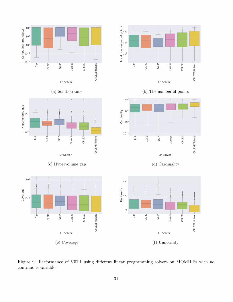
Figure 9 shows the performance of V5T1 on all 254 instances when the algorithm is built at thetop of different linear programming solvers. Overall, we observe that the solvers are competitive but‘CPLEXEfficient’ generates better approximations with respect to all quality indicators.

We now compare the performance of V1 to V5T1 with MDLS [39]. For this comparison, we haveused the C++ implementation of MDLS which is publicly available at http://prolog.univie.ac.

at/research/MDLS. It is worth mentioning that this implementation is problem-dependent in a sensethat some of its source/header files should be specifically defined for any problem that we are tryingto solve. Fortunately, we are able to employ MDLS for all 154 instances of knapsack problem . Thisis because in the available implementation, the corresponding header/source files for solving suchinstances exist.

We use the default setting of MDLS in which it repeats for 10 runs for each instance, and reportsthe results of each run. For comparison purposes, we accumulate the results of all 10 runs for eachinstance. We again impose a time limit of 120 seconds for different version of our algorithm but donot impose any time limit for MDLS since it naturally terminates within 120 seconds. Figure 10 showthe performance of V1 to V5T1 on the instances of the knapsack problem. Overall, we see that evenV1 outperforms MDLS.

29

V1 V2 V3 V4 V5 T1 V5 T2 V5 T3 V5 T4Algorithms

10−3

10−2

10−1

100

101

102

Compu

ting tim

e (Sec

.)

(a) Solution time

V1 V2 V3 V4 V5 T1 V5 T2 V5 T3 V5 T4Algorithms

100

101

102

103

Loca

l non

dominated

points

(b) The number of points

V1 V2 V3 V4 V5 T1 V5 T2 V5 T3 V5 T4Algorithms

100

101

102

Hype

rvolum

e ga

p

(c) Hypervolume gap

V1 V2 V3 V4 V5 T1 V5 T2 V5 T3 V5 T4Algorithms

100

101

102

Cardinality

(d) Cardinality

V1 V2 V3 V4 V5 T1 V5 T2 V5 T3 V5 T4Algorithms

10−2

10−1

100

Cove

rage

(e) Coverage

V1 V2 V3 V4 V5 T1 V5 T2 V5 T3 V5 T4Algorithms

10−1

100

101

102

Unifo

rmity

(f) Uniformity

Figure 8: Performance of V1 to V5T4 on MOMILPs with no continuous variables

30

Clp

GLPK

SCIP

Gurobi

CPLE

X

CPLE

XEfficie

nt

LP Solver

10−2

10−1

100

101

102

Compu

ting tim

e (Sec

.)

(a) Solution time

Clp

GLPK

SCIP

Gurobi

CPLE

X

CPLE

XEfficie

nt

LP Solver

101

102

103

Loca

l non

dominated

points

(b) The number of points

Clp

GLPK

SCIP

Gurobi

CPLE

X

CPLE

XEfficie

nt

LP Solver

100

101

Hype

rvolum

e ga

p

(c) Hypervolume gap

Clp

GLPK

SCIP

Gurobi

CPLE

X

CPLE

XEfficie

nt

LP Solver

10−1

100

101

102

Cardinality

(d) Cardinality

Clp

GLPK

SCIP

Gurobi

CPLE

X

CPLE

XEfficie

nt

LP Solver

10−1

100

Cove

rage

(e) Coverage

Clp

GLPK

SCIP

Gurobi

CPLE

X

CPLE

XEfficie

nt

LP Solver

100

101

102

Unifo

rmity

(f) Uniformity

Figure 9: Performance of V5T1 using different linear programming solvers on MOMILPs with nocontinuous variable

31

MDLS V1 V2 V3 V4 V5 T1Algorithms

10 3

10 2

10 1

100

101

102

Com

puting tim

e (Sec.)

(a) Solution time

MDLS V1 V2 V3 V4 V5 T1Algorithms

100

101

102

103

Local non

dominated

points

(b) The number of points

MDLS V1 V2 V3 V4 V5 T1Algorithms

100

101

102

Hypervolume ga

p

(c) Hypervolume gap

MDLS V1 V2 V3 V4 V5 T1Algorithms

10−1

100

101

102

Cardina

lity

(d) Cardinality

MDLS V1 V2 V3 V4 V5 T1Algorithms

10−2

10−1

100

101

Coverag

e

(e) Coverage

MDLS V1 V2 V3 V4 V5 T1Algorithms

100

101

102

103

Uniform

ity

(f) Uniformity

Figure 10: Performance comparison of V1 to V5T1 with MDLS on MOMILPs with no continuousvariable

32

V1 V2 V3 V4 V5 T1 V5 T2 V5 T3 V5 T4Algorithms

10−1

100

101

102

Compu

ting tim

e (Sec

.)

(a) Solution time

V1 V2 V3 V4 V5 T1 V5 T2 V5 T3 V5 T4Algorithms

101

102

103

104

Loca

l non

dominated

points

(b) The number of points

V1 V2 V3 V4 V5 T1 V5 T2 V5 T3 V5 T4Algorithms

10−1

100

101

Hype

rvolum

e ga

p

(c) Hypervolume gap

V1 V2 V3 V4 V5 T1 V5 T2 V5 T3 V5 T4Algorithms

10−2

10−1

100

101

Cardinality

(d) Cardinality

V1 V2 V3 V4 V5 T1 V5 T2 V5 T3 V5 T4Algorithms

10−3

10−2

10−1

Cove

rage

(e) Coverage

V1 V2 V3 V4 V5 T1 V5 T2 V5 T3 V5 T4Algorithms

100

101

102

103

Unifo

rmity

(f) Uniformity

Figure 11: Performance V1 to V5T4 on MOMILPs with more than two objectives

33

Clp

GLPK

SCIP

Gurobi

CPLE

X

CPLE

XEfficie

nt

LP Solver

10−2

10−1

100

101

102

Compu

ting tim

e (Sec

.)

(a) Solution time

Clp

GLPK

SCIP

Gurobi

CPLE

X

CPLE

XEfficie

nt

LP Solver

101

102

103

Loca

l non

dominated

points

(b) The number of points

Clp

GLPK

SCIP

Gurobi

CPLE

X

CPLE

XEfficie

nt

LP Solver

100

101

Hype

rvolum

e ga

p

(c) Hypervolume gap

Clp

GLPK

SCIP

Gurobi

CPLE

X

CPLE

XEfficie

nt

LP Solver

101

102

Cardinality

(d) Cardinality

Clp

GLPK

SCIP

Gurobi

CPLE

X

CPLE

XEfficie

nt

LP Solver

10−1

100

Cove

rage

(e) Coverage

Clp

GLPK

SCIP

Gurobi

CPLE

X

CPLE

XEfficie

nt

LP Solver

100

101

102

Unifo

rmity

(f) Uniformity

Figure 12: Performance of V5T1 using different linear programming solvers on MOMILPs with morethan two objectives

34

7.3 MOMILPs with more than two objective functions

In this section, we compare the performance of V1 to V5T4 on 60 instances of MOMILPs with p > 2and n1, n2 > 0, i.e., instances of mixed binary problems listed in Table 1. A run time limit of 2 minutesis imposed for all experiments in this section. We again note that (to the best of our knowledge) thereexists no exact solution approach for solving instances in this section. So, for each instance, we runV5T1 for 15 minutes and treat its outputs as the true nondominated frontier.

Figure 11 shows the performance of V1 to V5T4 for all 60 instances. Again, we observe that usingmore sophisticated versions and more number of threads can result in generating better approxima-tions. For example, we see from Figure 11c that the hypervolume gap is less than 1% on average forV5T4. Figure 12 shows the performance of V5T1 on all 5 instances when the algorithm is built at thetop of different linear programming solvers. Again, we observe that the solvers are competitive but‘CPLEXEfficient’ generates better approximations with respect to all quality indicators.

8 Final Remarks

We extended our recent algorithm for computing approximate nondominated frontiers of bi-objectivepure integer linear programs to multi-objective mixed integer linear programs with an arbitrary num-ber of objective functions. To the best of our knowledge, we are the first authors introducing afeasibility pump based heuristic for solving multi-objective mixed integer linear programs. In addi-tion to the feasibility pump method, the proposed algorithm exploits the underlying ideas of severalother algorithms in the literature of both single-objective and multi-objective optimization includinga weighted sum method, a local search approach, and a local branching method. The algorithm alsoemploys a decomposition technique for generating approximate nondominated points from differentparts of the criterion space. We showed numerically that: (1) the performance of the algorithm isalmost independent of the type of linear programming solver embedded in the algorithm; (2) Thealgorithm produces high-quality approximate nondominated frontiers in a short time; (3) It can natu-rally exploits parallelism and compute even better approximations if this option is activated; and (4)It outperforms MDLS on instances of multi-objective knapsack problem.

References

[1] Achterberg, T. and Berthold, T. (2007). Improving the feasibility pump. Discrete Optimization,4(1):77 – 86. Mixed Integer ProgrammingIMA Special Workshop on Mixed-Integer Programming.

[2] Aneja, Y. P. and Nair, K. P. K. (1979). Bicriteria transportation problem. Management Science,27:73–78.

[3] Berthold, T., Lodi, A., and Salvagnin, D. (2017). Ten years of feasibility pump andcounting. Preprint. http://cerc-datascience.polymtl.ca/wp-content/uploads/2017/08/

Technical-Report_DS4DM-2017-009.pdf.

[4] Boland, N., Charkhgard, H., and Savelsbergh, M. (2015a). A criterion space search algorithm forbiobjective integer programming: The balanced box method. INFORMS Journal on Computing,27(4):735–754.

35

[5] Boland, N., Charkhgard, H., and Savelsbergh, M. (2015b). A criterion space search algorithmfor biobjective mixed integer programming: The triangle splitting method. INFORMS Journal onComputing, 27(4):597–618.

[6] Boland, N., Charkhgard, H., and Savelsbergh, M. (2016a). The L-shape search method for triob-jective integer programming. Mathematical Programming Computation, 8(2):217–251.

[7] Boland, N., Charkhgard, H., and Savelsbergh, M. (2016b). The quadrant shrinking method:A simple and efficient algorithm for solving tri-objective integer programs. European Journal ofOperational Research. available online.

[8] Boland, N. L., Eberhard, A. C., Engineer, F. G., Fischetti, M., Savelsbergh, M. W. P., andTsoukalas, A. (2014). Boosting the feasibility pump. Mathematical Programming Computation,6(3):255–279.

[9] Bringmann, K. and Friedrich, T. (2010). Approximating the volume of unions and intersectionsof high-dimensional geometric objects. Computational Geometry, 43(6):601 – 610.

[10] Castillo Tapia, M. and Coello Coello, C. A. (2007). Applications of multi-objective evolutionaryalgorithms in economics and finance: A survey. In Evolutionary Computation, 2007. CEC 2007.IEEE Congress on, pages 532–539.

[11] Chalmet, L. G., Lemonidis, L., and Elzinga, D. J. (1986). An algorithm for bi-criterion integerprogramming problem. European Journal of Operational Research, 25:292–300.

[12] Coello Coello, C. A., Lamont, G. B., and Van Veldhuizen, D. A. (2007). Evolutionary Algorithmsfor Solving Multi-Objective Problems. Springer, New York.

[13] Dachert, K., Gorski, J., and Klamroth, K. (2012). An augmented weighted Tchebycheff methodwith adaptively chosen parameters for discrete bicriteria optimization problems. Computers &Operations Research, 39:2929–2943.

[14] Dachert, K. and Klamroth, K. (2014). A linear bound on the number of scalarizations needed tosolve discrete tricriteria optimization problems. Journal of Global Optimization, pages 1–34.

[15] Deb, K., Pratap, A., Agarwal, S., and Meyarivan, T. (2002). A fast and elitist multiobjectivegenetic algorithm: Nsga-ii. IEEE Transactions on Evolutionary Computation, 6(2):182–197.

[16] Dunning, I., Huchette, J., and Lubin, M. (2017). Jump: A modeling language for mathematicaloptimization. SIAM Review, 59(2):295–320.

[17] Dchert, K., Klamroth, K., Lacour, R., and Vanderpooten, D. (2017). Efficient computation of thesearch region in multi-objective optimization. European Journal of Operational Research, 260(3):841– 855.

[18] Ehrgott, M. (2005). Multicriteria optimization. Springer Berlin Heidelberg, second edition.

[19] Ehrgott, M. and Gandibleux, X. (2004). Approximative solution methods for multiobjectivecombinatorial optimization. Top, 12(1):1–63.

36

[20] Fischetti, M., Glover, F., and Lodi, A. (2005). The feasibility pump. Mathematical Programming,104(1):91–104.

[21] Fischetti, M. and Lodi, A. (2003). Local branching. Mathematical Programming, 98(1):23–47.

[22] Fischetti, M. and Salvagnin, D. (2009). Feasibility pump 2.0. Mathematical Programming Com-putation, 1(2):201–222.

[23] Kirlik, G. and Sayın, S. (2014). A new algorithm for generating all nondominated solutions of mul-tiobjective discrete optimization problems. European Journal of Operational Research, 232(3):479– 488.

[24] Koksalan, M. and Lokman, B. (2014). Finding nadir points in multi-objective integer programs.Journal of Global Optimization, pages 1–23.

[25] Lei, D. (2009). Multi-objective production scheduling: a survey. International Journal of Ad-vanced Manufacturing Technology, 43(9):926–938.

[26] Lian, K., Milburn, A. B., and Rardin, R. L. (2016). An improved multi-directional local searchalgorithm for the multi-objective consistent vehicle routing problem. IIE Transactions, 48(10):975–992.

[27] Lubin, M. and Dunning, I. (2015). Computing in operations research using Julia. INFORMSJournal on Computing, 27(2):238–248.

[28] Lust, T. and Teghem, J. (2010). The multiobjective traveling salesman problem: A survey anda new approach. In Coello Coello, C. A., Dhaenens, C., and Jourdan, L., editors, Advances inMulti-Objective Nature Inspired Computing, volume 272 of Studies in Computational Intelligence,pages 119–141. Springer Berlin Heidelberg.

[29] Ozlen, M., Burton, B. A., and MacRae, C. A. G. (2013). Multi-objective integer programming: Animproved recursive algorithm. Journal of Optimization Theory and Applications. 10.1007/s10957-013-0364-y.

[30] Ozpeynirci, O. and Koksalan, M. (2010). An exact algorithm for finding extreme supportednondominated points of multiobjective mixed integer programs. Management Science, 56(12):2302–2315.

[31] Pal, A. and Charkhgard, H. (2017). A feasibility pump and local search based heuristic for bi-objective pure integer linear programming. Preprint. http://www.optimization-online.org/DB_FILE/2017/03/5902.pdf.

[32] Paquete, L., Schiavinotto, T., and Stutzle, T. (2007). On local optima in multiobjective combi-natorial optimization problems. Annals of Operations Research, 156(1):83.

[33] Przybylski, A. and Gandibleux, X. (2017). Multi-objective branch and bound. European Journalof Operational Research, 260(3):856 – 872.

37

[34] Przybylski, A., Gandibleux, X., and Ehrgott, M. (2010a). A two phase method for multi-objectiveinteger programming and its application to the assignment problem with three objectives. DiscreteOptimization, 7(3):149 – 165.

[35] Przybylski, A., Gandibleux, X., and Ehrgott, M. (2010b). A two phase method for multi-objectiveinteger programming and its application to the assignment problem with three objectives. DiscreteOptimization, 7(3):149 – 165.

[36] Requejo, C. and Santos, E. (2017). A Feasibility Pump and a Local Branching Heuristics forthe Weight-Constrained Minimum Spanning Tree Problem, pages 669–683. Springer InternationalPublishing, Cham.

[37] Sayın, S. (2000). Measuring the quality of discrete representations of efficient sets in multipleobjective mathematical programming. Mathematical Programming, 87(3):543–560.

[38] Soylu, B. and Yıldız, G. B. (2016). An exact algorithm for biobjective mixed integer linearprogramming problems. Computers & Operations Research, 72:204 – 213.

[39] Tricoire, F. (2012). Multi-directional local search. Computers & Operations Research, 39(12):3089– 3101.

[40] Zhou, A., Qu, B.-Y., Li, H., Zhao, S.-Z., Suganthan, P. N., and Zhang, Q. (2011). Multiobjectiveevolutionary algorithms: A survey of the state of the art. Swarm and Evolutionary Computation,1(1):32–49.

[41] Zitzler, E., Brockhoff, D., and Thiele, L. (2007). The hypervolume indicator revisited: On thedesign of Pareto-compliant indicators via weighted integration. In Obayashi, S., Deb, K., Poloni,C., Hiroyasu, T., and Murata, T., editors, Evolutionary Multi-Criterion Optimization, volume 4403of Lecture Notes in Computer Science, pages 862–876.

[42] Zitzler, E., Thiele, L., Laumanns, M., Fonseca, C., and Grunert da Fonseca, V. (2003). Perfor-mance assessment of multiobjective optimizers: an analysis and review. Evolutionary Computation,IEEE Transactions on, 7(2):117–132.

38