fracking, renewables & mean field gameshow opec sets production. the organization of petroleum...

FRACKING, RENEWABLES & MEAN FIELD GAMES

PATRICK CHAN∗ AND RONNIE SIRCAR†

Abstract. The dramatic decline in oil prices, from around $110 per barrel in June 2014 toless than $40 in March 2016, highlights the importance of competition between different energysources. Indeed, the sustained price drop has been primarily attributed to OPEC’s strategic decisionnot to curb its oil production in the face of increased supply of shale oil in the US, spurred bythe technological innovation of “fracking”. We study how continuous time Cournot competitions,in which firms producing similar goods compete with one another by setting quantities, can beanalyzed as continuum dynamic mean field games. In this context, we illustrate how the traditionaloil producers may react in counter-intuitive ways in face of competition from alternative energysources.

1. Introduction. The recent rapid fall in the price of oil is arguably the biggestenergy story of the past two years. Back in June 2014, the price of Brent crude wasup around $115 per barrel. As of January 23, 2015, it had fallen by more than half,down to $49 per barrel, and fell into the $30 range in March 2016 (see Figure 1). The

Fig. 1: End of day Commodity Futures Price Quotes for Crude Oil. Source:www.nasdaq.com

dramatic decline in oil prices illustrates the evolution of the global energy market ascompetition between different energy sources expands. Indeed, the sustained pricedrop was prompted in large part by OPEC’s decision not to curb its oil productionin the face of increased supply of shale gas and oil in the US, itself arising fromtechnological advances such as hydraulic fracturing and horizontal drilling, collectivelyreferred to as fracking.

∗Applied and Computational Mathematics, Princeton University. ([email protected]).Work partially supported by NSF grant DMS-1211906.

†ORFE Department, Princeton University. ([email protected]). Work partially supported byNSF grant DMS-1211906.

1

www.nasdaq.com

mailto:[email protected]

mailto:[email protected]

2 Patrick Chan and Ronnie Sircar

The goal of the present paper is to explain how dynamic game theory, in particularmean field games proposed by Lasry and Lions [17] and Huang et al. [14, 15], can beused to explain some of the strategic interactions between various energy producers.

How OPEC sets production. The Organization of Petroleum Exporting Countries(OPEC) is a cartel of oil-producing nations that accounts for about 40% of the world’soil production. Comprising of twelve member countries (including key oil nations likeSaudi Arabia, Iran, Iraq, and the UAE), OPEC mandates to “coordinate and unifythe petroleum policies” of its members and to “ensure the stabilization of oil marketsin order to secure an efficient, economic and regular supply of petroleum to consumers,a steady income to producers, and a fair return on capital for those investing in thepetroleum industry.”1 OPEC typically meets twice a year to set production quotas.As with most commodities, the price of oil is mainly dictated by supply and demand.Since the supply of oil was determined in large part by OPEC, the higher they settheir quotas, the lower the oil price.

Oil prices had been high since 2010 through the middle of 2014, bouncing around$110 per barrel because of escalating oil consumption in countries like China andpolitical instability in key oil nations like Iraq. Given the high oil prices, manyenergy companies (most notably Chevron Corporation, Exxon Mobil Corp and Cono-coPhillips Co) found it profitable to begin extracting oil from difficult-to-drill places.In the United States, companies began using techniques like hydraulic fracturing andhorizontal drilling to extract oil from shale formations in North Dakota and Texas.

Plummeting oil price. Hydraulic fracturing, or “fracking”, is the process throughwhich oil and gas are released from shale deposits deep underground by means ofdrilling and injecting pressurized liquid made of water, sand, and chemicals. Ac-cording to the US Energy Information Administration, there are over 500,000 activenatural gas wells in the US as of 2011, adding significantly to the world oil supply. Toput this in context, the US fracking industry has added nearly 4 million extra barrelsof crude oil per day to the global market since 2008 (compared to global productionof about 75 million barrels per day). This surge in supply, together with a lack ofdemand due to sluggish global economic growth, led to a fall in oil price of nearly50% over the second half of 2014. As oil prices tumbled, most observers expected tosee OPEC, the world’s largest oil cartel, cut back on production to push prices backup.

OPEC’s war on fracking. This brings us to the OPEC Conference in Vienna on27 November 2014. Some countries, like Venezuela and Iran, wanted the cartel to cutback on production in order to boost the price. On the other side of the debate, SaudiArabia didn’t want to give up market share and refused to reduce production – inthe hopes that lower oil prices would help impede expansion of the fracking industry.In the end, despite the oversupply on the world market, OPEC failed to agree ona response and ended up keeping production unchanged. So the price of oil begandeclining even further.

The price of oil has hovered in the $40-55/barrel range for most of the first halfof 2015, but it is estimated that many fracking companies need prices above $60-80to break even. There is now speculation that many fracking operations may be forcedinto closure. The theory is that OPEC is now engaged in a “price war” with theUS frackers. Led by powerful oil nations such as Saudi Arabia, OPEC is seeking todrive the fracking industry out of business, once again regain its place as the world’s

1Source: http://www.opec.org/opec_web/en/publications/345.htm

http://www.opec.org/opec_web/en/publications/345.htm

Fracking, Renewables & Mean Field Games 3

pre-eminent source of oil, and stabilize oil prices well above the present level. This isthe central issue of blockading we want to model using dynamic game theory.

1.1. Competitive oligopolistic view. We take a competitive oligopolistic viewof an idealized global energy market, in which game theory describes the outcome ofcompetition. Oligopoly models of markets with a small number of competitive play-ers go back to the classical works of Cournot [5] and Bertrand [2] in the 1800s. TheCournot and Bertrand models differ on the assumptions about the strategic variablesa firm chooses to compete with its rivals. The Bertrand model assumes that firmscompete on price while the Cournot model assumes that the competition is on outputquantity. The Cournot framework of oligopoly is appropriate for energy productionin which major players determine their output relative to their production costs, as inthe expected scenario that OPEC will cut production in order to increase the marketprice of oil.

In the context of nonzero-sum dynamic games between N players, each withtheir own resources, the computation of a Nash equilibrium is a challenging problem,typically involving coupled systems of N nonlinear Hamilton-Jacobi-Bellman (HJB)partial differential equations (PDEs), with one value function per player. This isfurther complicated by the fact that the players’ resources are exhaustible and themarket structure changes over time as players deplete their reserves and exit themarket. Harris et al. [12] study a Cournot version of the problem, and Ledvina andSircar [18] study a similar problem in the Bertrand framework.

Meanwhile, mean field games proposed by Lasry and Lions [17] and independentlyby Huang et al. [14, 15] allow one to handle certain types of competition in the con-tinuum limit of an infinity of small players by solving a coupled system of two PDEs.The interaction here is such that each player only sees and reacts to the statisticaldistribution of the states or actions of other players. Optimization against the distri-bution of other players leads to a backward HJB equation; and in turn their actionsdetermine the evolution of the state distribution, encoded by a forward Kolmogorovequation. This continuum approximation allows for analytical and computationalresults which are hard to obtain from the N -player system.

Our goal is to extend the basic Cournot mean field game (MFG) model in [4],and study the competition between the traditional energy producers and alternativesources. In this setting, the economy is framed as a Cournot competition where themarket model is specified by inverse demand functions, which give prices as a functionof quantities produced. In the context of a global energy market, we model OPEC by acontinuum of oil producers with low costs of production, but each member nation hasa finite reserve. The other side of the economy is represented by an alternative energyproducer (e.g. the fracking industry in the US or renewable production such as fromsolar technology) with relatively costly production. However, the alternative energyproducer is distinguished from the traditional oil producers by its relative abundanceof production capacity. Throughout this paper, we make the simplifying assumptionthat the alternative energy source is inexhaustible relative to the traditional source.

“The Stone Age did not end for lack of stone, and the Oil Age will end long beforethe world runs out of oil.” With recent technological advances such as renewablesand fracking, this intriguing quote of former Saudi oil minister Sheikh Zaki Yamanimay not be far-fetched and the end of the traditional oil age may be upon us. In thispaper, our central innovation is to consider the interaction and competition betweentraditional and alternative energy producers. We do so by considering three distincttime scales representing different idealizations of the global energy market. Table


1 describes the three time scales under consideration and the main features of eachhorizon.

Table 1: Three distinct time scales representing different idealizations of the globalenergy market.

Horizon Global Energy Market

Long-term Over a longer horizon, alternative energy sources become more com-petitive as their production costs decrease further due to technologicaladvances. While traditional fossil fuels are not necessarily depleted,renewable energy gains considerable market share due to increasing(scarcity) costs of fossil fuel extraction. We study how the globaleconomy transitions from the traditional/exhaustible energy produc-tion to its renewable counterpart (Section 3).

Intermediate Over an intermediate horizon, the production of traditional energy(fossil fuels e.g. oil) is still the cheapest. However, alternative en-ergy sources (shale oil or solar power) are gaining market share dueto decreasing production costs. Traditional energy producers maystrategically increase their production rate to compete for marketshare with the alternative energy producers. This may be the logicbehind OPEC’s decision not to cut crude oil output. Section 1.3 be-low illustrates the issue of blockading in the simplest setting of staticgames. Competition between exhaustible fossil fuels and renewablealternatives is studied in a dynamic model in Section 4.

Short-term Over a short time frame, traditional energy sources are not going torun out. The major determinant of the energy price level is supplyshocks due to exploration successes, itself arising from investment inresearch and development. We model the joint strategic decision of(costly) exploration effort and production rate in this context (Section5).

1.2. Market Structure and Participants. Typically we are interested in com-petition between traditional oil producers and an alternative energy producer. In thissetting there is a continuum of traditional oil producers labelled by “position” x anddensity m(x). We denote the quantity of the traditional (resp. alternative) producersby q(x) (resp. q), and the average production of the traditional producers by Q:

Q =

∫q(x)m(x) dx.

The (Cournot) market structure is defined by a decreasing inverse demand function P .The price p = P (q+ ǫQ+ δq) received by an oil producer is decreasing in his own

production quantity q, the average quantity Q produced by the other players, and thequantity q of the alternative energy producer. Here ǫ, δ ≥ 0 are interaction parametersthat measure the impact of the other players. Similarly, the price p = P (q + δQ) re-ceived by the alternative energy producer is decreasing in his own production quantityq as well as the average production quantity Q of the oil producers.

Often we will take P to be linear and ǫ and δ to be equal to one to make variousformulas easier to read and for illustration. We note that Q is the average production


so the impact of the other players on the representative player’s price is different fromthe impact of his own price q even when ǫ = 1.

1.3. Static MFG and blockading. To illustrate the effect of blockading in thesimplest setting, we consider a static (one-period) competition between traditional oilproducers and an alternative energy producer. We consider linear inverse demandfunction P (ξ) = 1 − ξ. The producer at position x has cost of production c(x). Inaddition, there is an alternative energy producer with cost c0.

In a Nash equilibrium (q∗(x), q∗) for the “∞ + 1” players, each one maximizesprofit as a best response to the other players’ equilibrium strategies:

supq≥0

q(1− q −Q− q∗ − c(x)), supq≥0

q(1− q −Q− c0),

where now Q =∫q∗m. If there is an interior maximum (i.e. each player having

positive equilibrium production), then we have

(1.1) q∗(x) =1

2(1−Q− q∗ − c(x)) , q∗ =

1

2(1−Q− c0).

Integrating q∗ against m and solving for Q using the above expression for q∗ yields

Q =1

3(1− q∗ − 〈c〉) =

1

5(1 + c0 − 2〈c〉) , where 〈c〉 =

∫

R+

c(x)m(x) dx.

Consequently, from (1.1) we derive

q∗ =1

5(2− 3c0 + 〈c〉) , q∗(x) =

1

5

(1−

5

2c(x) + c0 +

1

2〈c〉

).

Blockading of the alternative producer occurs when q∗ ≤ 0, or equivalently whenc0 ≥ (2 + 〈c〉) /3 in terms of production costs. The interpretation is that the alterna-tive energy producer is blockaded when his cost c0 is too high compared to the averageproduction cost 〈c〉 of the traditional producers. In this case the alternative producerproduces nothing q∗ = 0, and the traditional producers take over the market

Q =1

3(1− 〈c〉) , which leads to q∗(x) =

1

3

(1−

3

2c(x) +

1

2〈c〉

).

In this case, we say that the alternative energy producer is blockaded from production.Figure 2 shows that as c0 decreases (representing increased competitiveness of thecostly alternative energy source), the traditional low-cost producer may strategicallychoose not the reduce production in an attempt to keep the alternative producerblockaded. In our context, this may be OPEC holding back on cuts in production todrive shale oil producers out of the market and into bankruptcy.

We study in Section 4 a dynamic version of this game incorporating exhaustibilityof the traditional fuel.

1.4. Related Literature. Our paper is related to two different strands of lit-erature: the literature of dynamic oligopoly with exhaustibility, and the literature onthe use of mean field games in economic applications.


(a) Types of game equilibrium in(〈c〉, c0) space

(b) Average production quantity Q

Fig. 2: Static Cournot duopoly with linear demand P (ξ) = 1 − ξ. When c0 is largerelative to fixed 〈c〉, the alternative energy producer is blockaded from production,and the traditional oil producers take over the entire market.

Dynamic Oligopoly. The study of static oligopoly models of markets with a smallnumber of competitive players goes back to the classical works of Cournot [5] andBertrand [2] in the 1800s. More recently, energy markets have been modeled throughdynamic games. Harris et al. [12] characterize a dynamic Cournot game in an oligopolymarket by systems of nonlinear Hamilton-Jacobi PDEs. Ledvina and Sircar [18] studythe corresponding Bertrand game in which firms compete with one another by settingprices. We refer to Dockner [8] for an introduction to the applications of dynamicgames in economics and management science.

Hotelling [13] introduced one of the first models for the management of an ex-haustible resource. In a monopoly setting, Hotelling solved a calculus-of-variationsproblem and showed that the marginal value of reserves grows at the discount ratealong the optimal extraction path, which is now referred to as Hotelling’s rule. Thecompetition between a single exhaustible producer and N−1 renewable producers hasbeen considered by Ledvina and Sircar [19]. This simplified setup provides insightsinto the effect of blockading: how low must oil reserves go before it becomes profitablefor the renewable producers to enter the market. It also leads to a modified piecewiseversion of Hotelling’s rule.

Other aspects of the exhaustibility issue are renewability and exploration. Forexample, while fossil fuels are ultimately exhaustible, they are also replenishable by(costly) exploration efforts. The optimal planning of exploration effort has been con-sidered by Pindyck [25] and many others in the monopoly context, and Ludkovskiand Sircar [21] in a dynamic duopoly. Dynamic Cournot games when the demandfunction is stochastic are studied in Ludkovski and Yang [24]. For a recent survey ofgame theoretic models for energy production, we refer to Ludkovski and Sircar [22].

Mean Field Games. Second, there is also a literature on the use of mean fieldgames to economic applications. Since the seminal papers by Lasry and Lions [17]and Huang et al. [14, 15], this approximation technique has attracted considerableinterest recently as the corresponding N -player dynamic games are almost always


intractable using PDE methods. In the context of energy production, Gueant etal. [10, 11] have considered a mean field version of a Cournot game with a quadraticcost function; while Chan and Sircar [4] apply asymptotic and numerical methods tostudy how substitutability affects the market equilibrium in Bertrand and Cournotmean field games.

There are many other applications of mean field games in economics, and we listonly a few. Lucas and Moll [20] study knowledge growth in an economy with manyagents of different productivity levels. In particular, what they call a “balanced growthpath” resembles our sustainable economy in Section 5. Carmona et al. [3] present amean field game model for analyzing systemic risk. Mean field games analysis has beenadopted to study the optimal execution problem in algorithmic trading by Jaimungaland Nourian [16]. For a comprehensive study of the uniqueness and existence ofequilibrium strategies of a general class of mean field games, including the linear-quadratic framework, we refer to Bensoussan et al. [1]. We explain the differencesbetween the type of problem considered in the bulk of this literature and our type ofproblem in Section 2.1, and what is known about existence and uniqueness for thiskind of system in Appendix A.

1.5. Organization and Results. We study the interaction between the tradi-tional and alternative energy producers from three perspectives: competition, transi-tion, and exploration.

In Section 2, we revisit the basic framework for dynamic Cournot mean fieldgames with exhaustible resources and extend the results of [4] to include nonlineardemand functions. Section 3 considers an economy in which the exhaustible producerscan transition to an alternative energy source (e.g. solar or hydroelectric power) whenthey run out of reserves. This essentially introduces a Neumann boundary condition tothe PDE problem. We provide explicit leading-order correction to the value functionin the regime of small exhaustibility.

Section 4 investigates the competitive interaction between the exhaustible oilproducers with an alternative energy producer, who has marginal cost of productionc > 0, but inexhaustible supplies. We shall see the blockading of the renewableproducer when his production cost c is high enough and when the exhaustible resourceis still abundant. Section 5 deals with exploration and exhaustibility. Incorporatingthe stochastic effect of resource exploration into the dynamic Cournot framework, westudy the equilibrium production rate and exploration effort in a sustainable economy.This corresponds to a steady-state solution to the MFG PDE problem. We concludein Section 6. Appendix A discusses an existence and uniqueness theorem for a classicalsolution to the type of MFG system considered here.

2. Dynamic Cournot model. The basic mean field game model in [4] will serveas a baseline for our analysis of competition between the traditional energy producersand the alternative sources. While the exposition there focuses on a Bertrand (price-setting) model, it is shown in their Appendix B that in the continuum mean fieldsetting, the dynamic Cournot and Bertrand games are identical. Since our focusin this paper is the global energy market in which the Cournot framework is moreappropriate, we elaborate on and extend the dynamic Cournot mean field game modelto nonlinear demand functions in this section. To introduce notation and ideas, weconcentrate in this section only on the exhaustible oil producers without competitionfrom the alternative producers, which are introduced in Section 3.


2.1. Dynamic continuum mean field games. In the dynamic problem, firmsproduce energy by depleting their reserves of a fossil fuel, and different producers havedifferent levels of initial reserves. When they exhaust their reserves, they no longerparticipate and the market shrinks. There is an infinity of players labelled by theirreserves x > 0, with initial density of reserves M(x). They choose production ratesqt which deplete the remaining reserve Xt; moreover the reserve level may be subjectto random fluctuations (e.g. due to noisy seismic estimation of the oil or gas well).The reserve level Xt follows the dynamics

dXt = −qt dt+ σ dWt,

as long as Xt > 0, and Xt is absorbed at zero. Here W is a standard Brownianmotion, and σ ≥ 0 is a constant.

A firm that starts with reserve x > 0 at time t ≥ 0 sets quantities to maximize thelifetime profit discounted at constant rate r > 0 over Markov controls qt = q(t,Xt),with the corresponding price pt = p(t,Xt) given by the inverse demand to be specifiedbelow. Hence the value function of the firm is defined by

(2.1) v(t, x) = supq

E

{∫ ∞

t

e−r(s−t)psqs1{Xs>0} ds

∣∣∣∣Xt = x

}, x > 0.

The game runs till some exhaustion time T (which may be infinite) when all producershave exhausted their reserves, and T has to be determined endogenously as part ofthe problem.

The price received by the player depends on his own production quantity qt aswell as the mean production rate Q(t), according to

(2.2) pt = P (qt + εQ(t)), Q(t) =

∫

R+

q(t, x)m(t, x) dx,

where m(t, x) denotes the density of producers’ reserves at time t > 0, and P is adecreasing inverse demand function. We note that the price received by a represen-tative producer depends on the other players through their mean production rate Q,and so the interaction is of mean field type. The parameter ε measures the degreeof interaction or product substitutability, in the sense that the price received by anindividual firm decreases as the other firms increase production of their goods.

In [4], the inverse demand function is taken to be linear: P (Q) = 1−Q. In thissection, we extend their results to nonlinear inverse demand function P of power type:

(2.3) P (Q) =

η1−ρ

(1−

(Qη

)1−ρ), ρ 6= 1,

η (log η − logQ) , ρ = 1.

The parameter ρ is known as the relative prudence. Notice that we recover the specialcase of linear demand by setting ρ = 0 and η = 1. Following [18], we focus on thecase where ρ < 1 in which the choke price P (0+) = η/(1− ρ) is finite. This family ofpricing function is shown in [12] to be particularly tractable for the computation ofNash equilibrium in the static Cournot game. It is further analyzed in [23].

2.2. Dynamic programming and the HJB equation. The HJB equationassociated to (2.1) is

(2.4) ∂tv +1

2σ2∂2

xxv − rv +maxq≥0

q (P (q + εQ(t))− ∂xv) = 0, x > 0,


where the inverse demand P is given by (2.3). Notice that the embedded optimiza-tion can be interpreted as a static profit maximization problem for a producer with(shadow) cost ∂xv facing competitors’ productionQ(t). The optimal production quan-tity q∗ is given (implicitly) by the first order condition

(2.5) P ′(q∗+εQ(t))q∗+P (q∗+εQ(t))−∂xv(t, x) = 0, Q(t) =

∫

R+

q∗(t, x)m(t, x) dx.

When a player runs out of reserves, he no longer produces or makes income, and so wehave the boundary condition v(t, 0) = 0. At the exhaustion time T , v(T, x) = 0, butas mentioned before, the terminal time T when all oil runs out has to be determinedendogenously.

Given the rate of depletion q∗(t, x), we can determine the ‘population dynamics’of the producers by the forward Kolmogorov equation

(2.6) ∂tm−1

2σ2∂2

xxm− ∂x (q∗m) = 0,

with m(0, x) = M(x). The system (2.4) and (2.6) is an example what Lasry andLions [17] have called a mean field game. The backward evolution equation (2.4)represents the firms’ decisions based on anticipating how the game unfolds in thefuture; and the forward evolution equation (2.6) represents where they actually endup, based on their strategic decision and initial distribution. The forward/backwardsystem of PDEs is coupled through the dependence of Q in the HJB equation (2.4)on m, and the dependence of q∗ in the forward Kolmogorov equation (2.6) on ∂xv.

Remark 2.1. After solving for the internal maximization provblem in the HJBequation (2.4), the system (2.4) and (2.6) is of the form

∂tv +1

2σ2∂2

xxv − rv +H(t, ∂xv, [h(∂xv)m]) = 0,(2.7)

∂tm−1

2σ2∂2

xxm− ∂xG (t, ∂xv, [h(∂xv)m]) = 0,

for some functions H, G and h. Here, H and G depend on h(∂xv)m nonlocally,specifically [h(∂xv)m] =

∫h(∂xv)mdx.

The vast majority of the MFG literature studies mean field game models of theform

∂tv +1

2σ2∂2

xxv − rv +H(t, x, ∂xv) = V [m],

∂tm−1

2σ2∂2

xxm− ∂x (G(t, x, ∂xv)) = 0,

(2.8)

where V [m] is a monotone operator. But in the systems (2.7) arising in this paper,the coupling between ∂xv and m is non-local.

The models leading to systems of the form (2.8) have interaction through thestates, namely

∫xm, whereas for Cournot oligopoly models, interaction is through the

controls, that is∫qm, which leads to equations of the form (2.7). However, motivated

by our previous paper [4], the recent preprint of Graber & Bensoussan [9] addressesexistence and uniqueness of a classical solution to systems of the type (2.7), specificallywhen the inverse demand function P , and hence h, is linear. We discuss in AppendixA how their theorem can be applied to validate the numerical work in the model weconsider in Section 4.


2.3. Small competition asymptotics. Solving this coupled system of equa-tions is highly non-trivial. In this section, we focus on the deterministic setting σ = 0.The main goal is to determine the principal effect of competitiveness on the marketequilibrium.

From the inverse demand function (2.2), we see that ε parameterizes the degree ofinteraction among firms; the limit ε = 0 corresponds to independent markets, whereeach firm has a monopoly in his own market. In the small competition regime, onecan formally look for an approximation to the PDE system of the form

v(t, x) = v0(t, x) + εv1(t, x) + ε2v2(t, x) + · · · ,

m(t, x) = m0(t, x) + εm1(t, x) + ε2m2(t, x) + · · · .

Solving for the value function v and the density m perturbatively leads to approxi-mations to q∗ and Q in (2.5):

q∗(t, x) = q0(t, x) + εq1(t, x) + · · · , Q(t) = Q0(t) + εQ1(t) + · · · .

2.3.1. Monopoly value function and production rate. The monopoly valuefunction v0 is determined by setting ε = 0 in the HJB equation (2.4), and afterperforming the maximization, we have:

(2.9) ∂tv0 − rv0 + C

(η

1− ρ− ∂xv0

)β

= 0, v0(t, 0) = 0,

where C = β−βη−ρ

1−ρ and β =2− ρ

1− ρ, and we recall that we only consider the cases

where ρ < 1. The solution to (2.9) is given in the following proposition, which can beverified by direct substitution.

Proposition 2.2. The leading order (monopoly) value function is time-independentv0(t, x) = v0(x), and it is implicitly given by

(2.10)βC

r

(1− ρ

η

)1−β

B

(1− ρ

η

( r

C

)1/βv1/β0 ;β, 0

)= x,

where the incomplete beta function B(z; a, b) is defined by

B(z; a, b) =

∫ z

0

ta−1(1− t)b−1 dt.

In particular, we recover the case of linear inverse demand studied in [4] if we setρ = 0 since in this case β = 2, B(z; 2, 0) = −z − log(1 − z), and so v0 can be writtenin terms of the Lambert-W function.

Production trajectory and Hotelling’s rule. In the monopoly case, the optimalproduction quantity q0 for each individual firm is given by setting ε = 0 in (2.5):

(2.11) P ′(q0)q0 + P (q0)− v′0 = 0.

It follows from (2.11) that

(2.12) q0(x) =

(P (0)− v′0(x)

βηρ

) 11−ρ

.


It is easy to show that v0(x) is an increasing concave function, with v0(0) = 0 andv0(∞) = η2(2 − ρ)−β/r. Therefore, v′0(x) is a decreasing function, with v′0(0) =P (0) = η

1−ρ and v′0(∞) = 0. Consequently, q0(x) is an increasing function of x, with

q0(0) = 0 and q0(∞) = η(2− ρ)−1

1−ρ . Therefore, players produce at a finite rate, andas they run out of reserves, they decrease their production rate to zero at x = 0.

Let x0(t;x) denote the optimal monopoly production trajectory starting from x:

x′0(t) = −q0(x0(t)), x0(0) = x, and define S(t) = v′0(x0(t)),

so S(t) is the shadow cost along the optimal production trajectory x0(t).Proposition 2.3. The classical Hotelling’s rule holds also for the continuum

mean field monopoly, i.e. the shadow cost grows at the discount rate r along theoptimal production trajectory: S ′(t) = rS(t). It follows that the market price P(t) =P (q0(x0(t))) satisfies the following linear ODE:

(2.13) P ′(t) = r

(P(t)−

η

2− ρ

).

Proof. First we write the monopoly ODE (2.9) as rv0 = q0(P (q0)− v′0), where q0satisfies the first order condition (2.11). Then differentiating the ODE with respectto x, and using (2.11), we obtain rv′0 = −q0v

′′0 . Now we compute the growth rate of

the shadow cost S(t) along the optimal production trajectory:

S ′(t) =d

dtv′0(x0(t)) = −v′′0 (x0(t)) q0 (x0(t)) = rS(t).

By direct calculation, the market price is a linear function of v′0: P (q0(x)) =η+v′

0(x)2−ρ .

It follows easily that P also satisfies a linear ODE, which is given by (2.13).

2.3.2. Monopoly exhaustion times. We define the hitting time τ : R+ → R+

to be the time to exhaustion in the deterministic monopoly market starting at initialreserve x:

(2.14) τ(x) = inf{t ≥ 0 | x0(t;x) = 0}.

Even though there does not seem to be an explicit expression for the reserve trajectory,the exhaustion time τ(x) can be given explicitly in the following proposition.

Proposition 2.4. The exhaustion time τ(x) is given explicitly by

(2.15) τ(x) =1

rlog

(P (0)

v′0(x)

).

Moreover, the exhaustion time τ can be inverted in closed-form to give

(2.16) τ−1(t) =βC

rP (0)β−1B

(1− e−rt;β, 0

).

Proof. From the definition (2.14) of τ(x), and using that v′0 is a monotonicfunction with v′0(0) = P (0), we write

τ(x) = inf{t ≥ 0 | v′0(x0(t)) = P (0)} = inf{t ≥ 0 | v′0(x)ert = P (0)},


where we have used Hotelling’s rule given in Proposition 2.3. The expression (2.15)follows. From the HJB equation (2.9), we derive

v0(x) =C

rP (0)β

(1− e−rτ(x)

)β.

Plugging this into the expression (2.10), and identifying x = τ−1(t) lead to (2.16).In the special case of linear inverse demand (where ρ = 0 and η = 1), we

have τ(x) = −r−1 log [−W(θ(x))], where W is the Lambert-W function, and θ(x) =−e−2rx−1, which recovers the one found in [4].

When the initial density M(x) has compact support [0, xmax], all oil reserves areexhausted at finite time T = τ(xmax); otherwise T = ∞.

2.3.3. Monopoly density function. In the deterministic monopoly setting,the forward Kolmogorov equation (2.6) reads

(2.17) ∂tm0 − ∂x[q0m0] = 0, m0(t, x) = M(x).

Proposition 2.5. The monopoly density is given by

(2.18) m0(t, x) =q0(τ−1 (t+ τ(x))

)

q0(x)M(τ−1 (t+ τ(x))

)=

d

dxF (τ−1(t+ τ(x))),

where F denotes the cumulative distribution function (CDF) of the initial density M .Moreover, the proportion η0 : R+ → [0, 1] of remaining firms is given by

η0(t) =

∫

R+

m0(t, x) dx = 1− F (τ−1(t)).

Proof. The explicit solution to (2.17) follows from the method of characteristics;while the second expression for m0 in (2.18) follows from straightforward manipula-tion. The computation of η0 follows similarly to [4, Proposition 6].

2.3.4. First order asymptotics. Let G be the supremum in the PDE (2.4):G(ε) = maxq≥0 q (P (q + εQ)− ∂xv). The first order condition is given in (2.5), andso, to first order in ε, we have G ≈ G(0) + εG′(0), where

G′(0) = (P (q0)− v′0)q1 + q0(q1 +Q0)P′(q0)− q0∂xv1 = q0 (Q0P

′(q0)− ∂xv1) .

This leads to the equation satisfied by the first order correction v1:

∂tv1 − rv1 − q0∂xv1 = −q0P′(q0)Q0, v1(t, 0) = 0.

Proposition 2.6. The first-order correction to the value function v1 is given by

v1(t, x) = −η

2− ρ

∫ τ(x)

0

(e−rs − e−rτ(x)

)Q0(t+ s) ds.

Proof. The proof follows similarly to [4, Proposition 8].


Clearly v1 < 0, so that competition reduces the value function from the monopolylimit v0, as is expected. The first order correction q1 to the optimal productionquantity is

(2.19) q1 =∂xv1 −Q0 (P

′(q0) + q0P′′(q0))

2P ′(q0) + q0P ′′(q0)=

∂xv1 − (1− ρ)Q0P′(q0)

(2− ρ)P ′(q0).

The first-order correction to density m1 satisfies the following equation

∂tm1 − ∂x [q0m1 + q1m0] = 0, m1(0, x) = 0.

Proposition 2.7. The first-order correction to density m1 is given by

m1(t, x) =

∫ t

0

q0 (x0(s− t;x))

q0(x)g (s, x0(s− t;x)) ds,

where the inhomogeneous term is given by g = ∂xq1m0 + q1∂xm0.Proof. The proof follows similarly to [4, Proposition 9].The following proposition demonstrates that the principal effect of competitive

interaction is that firms slow down production and increase the exhaustion time.Proposition 2.8. For concave pricing functions P (i.e. ρ < 0), the first order

correction q1 to the equilibrium production rate is negative.Proof. From the expression (2.19) for q1, it suffices to show that

∂xv1 − (1− ρ)Q0P′(q0) ≥ 0.

Indeed, defining F = βq0 [∂xv1 − (1− ρ)Q0P′(q0)], a straightforward calculation leads

to

F (t, x) = −rv′0(x)

∫ τ(x)

0

Q0(t+ s) ds+ (1− ρ)Q0(t) (P (0)− v′0(x)) .

One can readily check that F (t, 0) = 0 and ∂xF (t, x) ≥ 0 for concave P , and so from(2.19), q1 ≤ 0.

3. Transition to renewable resources. In this section, we consider a modelin which the exhaustible producers can switch to a more expensive alternative energysource (e.g. solar or hydroelectric power) when they run out of reserves. This modelcorresponds to the long horizon in Table 1. This yields a continuum mean field versionof the continuous-time Cournot model of Harris et al. [12]. In the context of energyproduction, resources, such as oil or natural gas, have finite supply, and exhaustibilityenters as boundary conditions for the PDEs. As we shall see, this essentially intro-duces a Neumann boundary condition to the PDE problem. We suppose there is analternative, but costly, technology (for example solar power), and study the systemusing asymptotic approximation. In the regime of small costs for the alternative,the first order correction to the value function satisfies a partial integro-differentialequation which is explicitly solvable.

3.1. Deterministic model setup. The energy market is modeled by a Cournotgame which is specified by the inverse demand: P (q,Q) = 1 − q −Q, where Q is themean energy production (from both traditional and alternative sources). A firm with


reserves x > 0 at time t ≥ 0 sets quantities to maximize lifetime discounted profits.Its value function is given by

(3.1) v(t, x) = supq

∫ ∞

t

e−r(s−t)psqs1{Xs>0} ds, Xt = x,

subject to the deterministic dynamics dXt = −qt dt.The HJB equation associated to (3.1) reads

∂tv − rv +maxq≥0

q (1− q −Q− ∂xv) = 0.

Plugging in the optimal strategy (in feedback form)

(3.2) q∗(t, x) =1

2(1−Q(t)− ∂xv(t, x)) ,

the HJB equation becomes

(3.3) ∂tv − rv +1

4(1−Q(t)− ∂xv(t, x))

2= 0.

On hitting the boundary x = 0, the player switches to an alternative inexhaustiblesource at marginal cost of production c. Playing against the mean production Q, hisequilibrium strategy is q∗(t, 0) = 1

2 (1 − Q − c). Assuming continuity of the equilib-rium production rates qt up to the boundary x = 0 leads to the Neumann boundarycondition ∂xv(t, 0) = c. The interpretation is that, on running out of the exhaustibleresource, the shadow cost ∂xv(t, x) of the player turns into the real cost c.

The mean production Q(t) comes from two sources: the exhaustible and inex-haustible parts. We assume that no player produces from the more expensive sourceas long as the cheaper one is available. Thus we can write

(3.4) Q(t) =1

2(1−Q(t)− c) (1− η(t)) +

∫

R+

q∗(t, x)m(t, x) dx,

where η is the proportion of players using the cheap energy source:

(3.5) η(t) =

∫

R+

m(t, x) dx,

and so (1−η) is the fraction of firms who have exhausted their traditional fuel reservesand are now producing from the alternative inexhaustible source at marginal cost c.Solving for Q in (3.4), and using (3.2), we obtain

(3.6) Q =1

3

(1− c(1− η)−

∫

R+

m∂xv dx

).

The forward Kolmogorov equation for m is

(3.7) ∂tm−1

2∂x ((1−Q− ∂xv)m) = 0,

with m(0, x) = M(x).

3.2. Small cost expansion.


Inexhaustible limit. In the limit where c = 0, the firms are indifferent to usingoil or alternative energy sources, and so costless energy is effectively inexhaustible.Consequently, the value function v0 is a constant. From (3.6) with c = 0 and ∂xv0 = 0,we derive a constant mean production Q0 = 1/3, which from the HJB equation (3.3)gives v0(t, x) = (9r)−1, also satisfying the boundary condition ∂xv0(t, 0) = 0. From(3.7), the density m is transported at constant speed m0(t, x) = M (x+ t/3).

We are interested in the case when c is small but non-zero. To this end we formallylook for an expansion in the small c regime:

v(t, x) = v0(t, x) + cv1(t, x) +O(c2),

m(t, x) = m0(t, x) + cm1(t, x) +O(c2).(3.8)

Of course, we have just found that v0 is independent of t and x and is given by (9r)−1.First order correction: value function. Plugging the formal expansion (3.8) into

the HJB equation (3.3) we get

∂tv1 − rv1 −1

3(Q1 + ∂xv1) = 0,

with ∂xv1(t, 0) = 1. Here Q1 is the first order correction to the mean production,given by

Q1 = −1

3

(1− η0 +

∫

R+

m0∂xv1 dx

).

Therefore, we obtain the partial integro-differential equation (PIDE) for v1

(3.9) ∂tv1 − rv1 −1

3∂xv1 +

1

9

(1−

∫

R+

m0(1− ∂xv1) dx

)= 0, ∂xv1(t, 0) = 1.

By considering an additively separable solution of the form v1(t, x) = f(x)+ g(t), thesolution to the above PIDE can be readily computed:

(3.10) v1(t, x) = −1

3re−3rx −

∫ t

0

I(s)er(t−s) ds,

where I(t) =1

9

(1−

∫ ∞

0

M(x+ t/3)(1− e−3rx

)dx

). That v1 is additively separa-

ble simplifies the expression for Q1 considerably:

(3.11) Q1(t) = −1

3

(1− η0 +

∫

R+

m0∂xv1 dx

)= −3I(t).

In particular, we see that Q1 is always negative. The economic interpretation isthat increasing the costs of inexhaustible energy source slows down production of theexhaustible one. From (3.2), we can compute the equilibrium production rate:

q∗(t, x) =1

3−

c

2

(Q1(t) + e−3rx

)+O(c2).

First order correction: density. The first order correction to density m1 satisfies

(3.12) ∂tm1 −1

3∂xm1 +

1

2∂x ((Q1 + ∂xv1)m0) = 0, m1(0, x) = 0.

Having already solved for v1, we can write down the solution analytically

(3.13) m1(t, x) =

∫ t

0

h

(s, x+

t− s

3

)ds, h(t, x) = −

1

2∂x ((Q1 + ∂xv1)m0) .


3.3. Numerical illustration. We illustrate the effect of exhaustibility using anumerical example. Suppose the initial distribution of reserves is given by an expo-nential distribution with parameter λ (i.e. M(x) = λe−λx). Then we can computethe value function correction

v1(t, x) = −1

9

(ert − 1

)(1

r−

3e−λt/3

λ+ 3r

)−

e−3rx

3r,

and the density correction

m1(t, x) =1

2λe−λ(x+t/3)

(r(3− 3e−λt/3

)

λ+ 3r+

(λ + 3r) (1− e−rt) e−3rx

r−

λt

3

).

The leading order correction to the mean production rate is

Q1(t) = −1

3

(1−

3re−λt/3

λ+ 3r

).

Observe that the correction to the mean quantity Q1 is always negative, in otherwords, exhaustibility shows down production, as shown in Figure 3.

c � 0

c � 0.2

c � 0.4

c � 0.6

0 1 2 3 4t

0.05

0.10

0.15

0.20

0.25

0.30

0.35

Q0+cQ1

(a) Mean production

c � 0

c � 0.2

c � 0.4

c � 0.6

2 4 6 8 10t

0.2

0.4

0.6

0.8

1.0

✁

(b) Proportion of exhaustible firms

Fig. 3: Effects of exhaustibility when the exhaustible producers can transition toproduction of renewable resources, parameters used for numerical simulation are λ = 1and r = 0.2.

3.4. Variable production costs. We illustrate that the technique of asymp-totic expansion can be applied to the variable production cost model in [6]. In theirsetting, instead of an abrupt transition to the alternative technology, a firm’s marginalproduction cost c(x) gradually increases up to c as the traditional energy reserve runsout x → 0. For illustrative purpose, we will take the variable production costs to bec(x) = ce−γx. The interpretation is that the exhaustible producer has non-zero cost ofextraction; in particular, as reserves begin to run out, costs for exhaustible producersoften increase (deeper drilling, more expensive extraction technology required), andthe exhaustible producer may choose to invest in R&D (research and development,including exploration) which adds to the marginal production costs.

Model setup. With non-zero production cost c(x), the value function of a repre-sentative firm is

(3.14) v(t, x) = supq

∫ ∞

t

e−r(s−t)(ps − c(Xs))qs1{Xs>0} ds, Xt = x,


subject to the dynamics dXt = −qt dt. The associated HJB equation is

(3.15) ∂tv − rv +maxq≥0

q (1− q −Q− ∂xv − c(x)) = 0,

with ∂xv(t, 0) = 0. The forward Kolmogorov equation for m is

(3.16) ∂tm−1

2∂x ((1−Q− ∂xv − c(x))m) = 0,

with m(0, x) = M(x), where the mean production Q(t) comes from both the ex-haustible and inexhaustible producers:

(3.17) Q =1

3

(1− c(1− η)−

∫

R+

m(∂xv + c(x)) dx

).

Small exhaustibility expansion. We formally look for an asymptotic expansion(3.8) in the small c regime. The inexhaustible limit c = 0 in the present model admitsa solution of a constant mean production Q0 = 1/3 with v0(t, x) = (9r)−1. Thedensity m0 is transported at constant speed m0(t, x) = M (x+ t/3). The leading-order corrections to the value function and density in the expansion (3.8) are givenby the following proposition.

Proposition 3.1. The leading-order correction to the value function v1 is addi-tively separable:

v1(t, x) = f(x) + g(t), where(3.18)

f(x) =3re−γx + γe3rx

9r2 + 3γr, g(t) =

1

3

∫ t

0

Q1(s)er(t−s) ds,(3.19)

Q1(t) = −1

3

(1−

∫

R+

M(x+ t/3)(1− e−γx − f ′(x)

)dx

).(3.20)

Moreover, the leading-order correction to the density m1 is given explicitly by(3.21)

m1(t, x) =

∫ t

0

h

(s, x+

t− s

3

)ds, h(t, x) = −

1

2∂x((Q1(t) + f ′(x) + e−γx

)m0

).

Proof. Plugging the formal expansion (3.8) into the HJB equation (3.15) we get

∂tv1 − rv1 −1

3

(Q1 + ∂xv1 + e−γx

)= 0,

with ∂xv1(t, 0) = 0. Here Q1 = −1

3

(1− η0 +

∫

R+

m0(∂xv1 + e−γx) dx

)is the first

order correction to the mean production. Therefore, we obtain the PIDE for v1:

∂tv1−rv1−1

3∂xv1+

1

9

(1−

∫

R+

m0(1− ∂xv1 − e−γx) dx

)=

1

3e−γx, ∂xv1(t, 0) = 0.

By considering the additively separable solution of the form (3.18), the solution tothe above PIDE can be readily computed to give (3.19) and (3.20).

As for the density, the first order correction m1 satisfies

∂tm1 −1

3∂xm1 +

1

2∂x((Q1 + ∂xv1 + e−γx

)m0

)= 0, m1(0, x) = 0.

Using the method of characteristics, we obtain the solution (3.21) analytically.Notice in particular that as the transition rate γ goes to infinity, the total pro-

duction rate Q1 in this case reduces to (3.11) as 1− e−γx − f ′(x) →γ→∞

1− e−3rx.


Numerical illustration. We illustrate the effect of exhaustibility using a numericalexample, where we assume that the initial reserves have an exponential density withparameter λ. Figure 4 shows the effect of the transition rate γ on the mean productionrate Q ≈ Q0 + cQ1. Notice that a smoother transition (i.e. decreasing γ) leads tohigher production rate.

Fig. 4: Effect of the transition rate γ on the mean production rate Q ≈ Q0 + cQ1.Parameters used are r = 0.2, λ = 1, c = 0.2.

4. Competition with a renewable Producer. In this section we consider thecompetition between the traditional oil producers with an alternative energy producer.This model corresponds to the intermediate time horizon in Table 1. The economyconsists of a continuum of firms depleting a non-renewable energy source with zeromarginal cost, and an alternative producer with inexhaustible reserves, but highercost of production c > 0. This corresponds to sustainable production from “green”sources (e.g. solar power, or to leading order approximation, the fracking industryin the US). The two classes of producers compete against each other through theCournot game equilibrium.

For the exhaustible producers, the remaining reserves (Xt) follow the dynamics

dXt = −qt dt+ σ dWt,

as long as Xt > 0, where W is a standard Brownian motion and qt = q(t,Xt) is hisrate of production at time t. Each exhaustible producer has oil resources which heextracts at zero costs, and which is subject to random fluctuation (e.g. due to noisyseismic estimates of oil reserves). When he runs out, he cannot produce anymoreand we have q(t, 0) = 0. The renewable player produces from an alternative sourcewhich is expensive but abundant: his marginal cost of production is c > 0. His rateof production is denoted by q(t).

The Cournot market is specified by linear inverse demand functions. The in-verse demand faced by an exhaustible producer producing at rate q unit is given byP (q, q, Q) = 1− q− δq − εQ, where Q is the mean production rate of the exhaustibleproducers, and q is the production rate of the renewable producer. The inverse de-mand faced by the renewable producer is similarly given by P (q, Q) = 1−q−δQ. Hereε is the interaction parameter between exhaustible producers, and δ is the interactionparameter between exhaustible producers and the renewable producer.


The value functions for the traditional and alternative producers are their dis-counted lifetime profit, respectively given by:

v(t, x) = supq≥0

E

{∫ ∞

t

e−r(s−t)qsps1{Xs>0} dt

∣∣∣∣Xt = x

},

g(t) = supq≥0

∫ ∞

t

e−r(s−t)qs(ps − c)1{η(s)>0} ds+

∫ ∞

t

e−r(s−t) 1

4(1− c)21{η(s)=0} ds,

(4.1)

where η is the fraction of exhaustible producers with reserves remaining, given by(3.5). The second term in the definition of g expresses that the renewable producerhas a monopoly when all the exhaustible producers are out of reserves.

We also stress that q must be non-negative: for large enough c, we will see thatthe renewable player is blockaded in that his cost of producer is so high and hiscompetitors’ reserves of the cheaper resource are so plentiful, that his equilibriumstrategy is not to produce anything until the exhaustible producers have run downtheir reserves some more. When c = 1, the renewable player never participates in thegame, and the above model reduces to the standard Cournot mean field game studiedin Section 2.

Dynamic programming and HJB equations. The HJB equations associated to(4.1) read

∂tv +1

2σ2∂2

xxv + supq

[q (1− q − εQ(t)− δq(t)− ∂xv)] = rv,

g′(t) + supq

[q (1− q − δQ(t)− c)] = rg.(4.2)

From the optimal feedback control q∗(t,Xt) of the exhaustible producer, the densitym of reserves Xt follows the forward Kolmogorov equation

(4.3) ∂tm−1

2σ2∂2

xxm− ∂x (q∗m) = 0,

with m(0, x) = M(x). The total production by exhaustible producer is given by

(4.4) Q(t) =

∫

R+

q∗(t, x)m(t, x) dx.

(a) If the renewable producer is not blockaded, the feedback production rates are

q∗nb(t, x) =1

4

(2− δ − (2ε− δ2)Q(t) + δc− 2∂xv

), q∗(t) =

1

2(1− δQ(t)− c) ,

and the HJB equations become

∂tv +1

2σ2∂2

xxv +1

16

(2− δ − (2ε− δ2)Q(t) + δc− 2∂xv

)2= rv,

g′(t) +1

4(1− δQ(t)− c)

2= rg.

(b) If the renewable producer is blockaded, we have q∗ = 0 and

q∗b (t, x) =1

2(1− εQ(t)− ∂xv) .

In this case the HJB equation becomes

∂tv +1

2σ2∂2

xxv +1

4(1− εQ(t)− ∂xv)

2= rv, g′(t) = rg.


Forward Kolmogorov equation. Combining the two cases, we can write the forwardKolmogorov equation of the reserves density as

(4.5) 0 = ∂tm−1

2σ2∂2

xxm− ∂x [m (1Bq∗b (t, x) + 1

cBq

∗nb(t, x))] ,

where 1B is the blockading indicator function.

4.1. Numerical solutions. To study the full MFG equation system (4.2) and(4.5), we need to solve a coupled system of forward/backward PDE system with afree boundary. We propose an iterative algorithm to calculate the MFG solution andoptimal production rate. Starting with an initial guess Q0 for the total production,we follow for n = 1, 2, . . .

Step 1. Given the mean production Qn−1 from the previous iteration, solve theoptimal control problem by numerically solving the HJB equations:(a) The optimal strategy of the renewable producer is simply

qn(t) =1

2

(1− δQn−1(t)− c

)+.

The renewable producer is “blockaded” whenever 1− δQ(t)− c < 0.(b) The exhaustible producer solves the optimal control problem

∂tvn +

1

2σ2∂2

xxvn +

1

4

(1− εQn−1(t)− ∂xv

n)2

1B

+1

16

(2− δ − (2ε− δ2)Qn−1(t) + δc− 2∂xv

n)2

1cB = rvn.

The feedback production strategy of the exhaustible producer is

qn(t, x) =1

2

(1− εQn−1(t)− ∂xv

n)1B+

1

4

(2− δ − (2ε− δ2)Qn−1(t) + δc− 2∂xv

n)1cB.

Step 2. Given the optimal production strategy qn, we can solve the forward Kol-mogorov equation

∂tmn −

1

2σ2∂2

xxmn − ∂x [m

nqn] = 0.

and determine the nth-iteration mean production Qn(t) =

∫

R+

qn(t, x)mn(t, x) dx.

As observed in [4], it is computationally convenient to consider the tail distributionfunction

(4.6) η(t, x) =

∫ ∞

x

m(t, y) dy.

The forward Kolmogorov equation in terms of η reads

∂tη(t, x)−1

2σ2∂2

xxη(t, x)− q(t, x)∂xη(t, x) = 0,

with initial condition (4.6) evaluated at t = 0, which allows us to handle point massesin the initial distribution M .

4.2. Results and discussion. We take the deterministic setting σ = 0 andchoose ε = δ = 1 for the following numerical illustrations.


Initialization and convergence of algorithm. The initial guess of the mean pro-duction Q0 is taken to be the explicit result (2.10) derived in the context of monopolyCournot competition (without the renewable producer). We observe that our itera-tive algorithm converges rapidly, typically within 10 iterations. From the left panelof Figure 5, we notice that the exhaustible producers slow down production in thepresence of a renewable competitor.

Blockading of renewable producer. If the constant marginal cost of production cis high enough, the renewable producer can be blockaded and produces nothing. Theidea is that when the marginal cost of production is high, and when the exhaustibleresource is plentiful, it may be advantageous for the renewable producer to holdback production and wait until the exhaustible players diminish their reserves. Wesee numerical evidence that blockading occurs when the marginal cost of productionc = 0.9.

2 4 6 8 10t

0.05

0.10

0.15

0.20

Q

(a) Exhaustible producers

2 4 6 8 10t

0.01

0.02

0.03

0.04

0.05

q�

(b) Renewable producer

Fig. 5: Production rates for the exhaustible (left) and renewable (right) producers.Notice the renewable producer is blockaded until about t = 1.5. The parameter areε = δ = 1, r = 0.2,M ∼ Beta(2, 4) and c = 0.9.

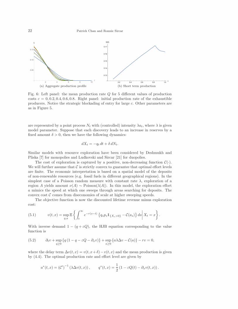
4.3. Strategic blockading entry of renewable resources. We now returnto OPEC’s strategic decision not to curb its oil production in face of increased supplyof shale gas and oil in the US. In Figure 6, we consider the mean production rate Q ofthe exhaustible producers when they are rivaled with an alternative source of differentmarginal costs c. The left panel shows the production profile Q(t) over time; while theright panel plots the short term production Q(0) as a function of the renewable energycost c. When c = 1, we know that the alternative energy producer does not participateand the traditional energy producers have the entire market to themselves. However,we see that as c decreases from 1, the exhaustible producers may strategically increasetheir mean production in the short run (and hence driving energy price down) to keepthe renewable energy out of the market. Therefore, our model is capable of providinga dynamical explanation to OPEC’s decision to maintain oil production in order tocompete for market share with the fracking industry in the US.

5. Resource Discovery. In this section, we study the stochastic effect of re-source exploration in dynamic Cournot mean field game models of exhaustible re-sources. This model corresponds to the short horizon in Table 1. The exhaustibleproducers may invest in exploration, with effort level indicated by at ≥ 0 and costC(at). The production capacity Xt decreases at a (controlled) production rate qt ≥ 0,and increases through jumps thanks to discrete new discoveries. Exploration successes


2 4 6 8 10t

0.05

0.10

0.15

Q

(a) Aggregate production profile

0.2 0.4 0.6 0.8 1.0c

0.13

0.14

0.15

0.16

0.17

Q(0)

(b) Short term production

Fig. 6: Left panel: the mean production rate Q for 5 different values of productioncosts c = 0, 0.2, 0.4, 0.6, 0.8. Right panel: initial production rate of the exhaustibleproducers. Notice the strategic blockading of entry for large c. Other parameters areas in Figure 5.

are represented by a point process Nt with (controlled) intensity λat, where λ is givenmodel parameter. Suppose that each discovery leads to an increase in reserves by afixed amount δ > 0, then we have the following dynamics:

dXt = −qt dt+ δ dNt.

Similar models with resource exploration have been considered by Deshmukh andPliska [7] for monopolies and Ludkovski and Sircar [21] for duopolies.

The cost of exploration is captured by a positive, non-decreasing function C(·).We will further assume that C is strictly convex to guarantee that optimal effort levelsare finite. The economic interpretation is based on a spatial model of the depositsof non-renewable resources (e.g. fossil fuels in different geographical regions). In thesimplest case of a Poisson random measure with constant rate λ, exploration of aregion A yields amount ν(A) ∼ Poisson(λ|A|). In this model, the exploration efforta mimics the speed at which one sweeps through areas searching for deposits. Theconvex cost C comes from diseconomies of scale at higher sweeping speeds.

The objective function is now the discounted lifetime revenue minus explorationcost:

(5.1) v(t, x) = supq,a

E

{∫ ∞

t

e−r(s−t){qsps1{Xs>0} − C(as)

}ds

∣∣∣∣Xt = x

}.

With inverse demand 1 − (q + εQ), the HJB equation corresponding to the valuefunction is

(5.2) ∂tv + supq≥0

{q (1− q − εQ− ∂xv)}+ supa≥0

{aλ∆v − C(a)} − rv = 0,

where the delay term ∆v(t, x) = v(t, x+ δ)− v(t, x) and the mean production is givenby (4.4). The optimal production rate and effort level are given by

a∗(t, x) = (C′)−1

(λ∆v(t, x)) , q∗(t, x) =1

2(1− εQ(t)− ∂xv(t, x)) .


Given the optimal controls, the population dynamics m(t, x) is governed by the for-ward Kolmogorov equation:(5.3)∂tm(t, x)− ∂x (q

∗(t, x)m(t, x)) − λ {a∗(t, x− δ)m(t, x− δ)− a∗(t, x)m(t, x)} = 0.

Note that the introduction of random jumps leads to a system of non-local PDEs.

5.1. Sustainable economy. Motivated by what Lucas and Moll [20] call a “bal-anced growth path”, we look for stationary solution to the above mean field gameequation system. The interpretation is a sustainable energy market in which resourceextraction is balanced by the exploration successes. The stationary equations are

rv(x) = supq≥0

{q (1− q − εQ− v′(x))}+ supa≥0

{aλ∆v − C(a)} ,

0 = −d

dx(q∗(x)m(x)) − λ {a∗(x− δ)m(x − δ)− a∗(x)m(x)} ,

a∗(x) = (C′)−1

(λ∆v(x)) , q∗(x) =1

2(1− εQ− v′(x)) , Q =

∫

R+

q∗(x)m(x) dx.

(5.4)

5.2. Computational algorithm. Following [21], we take power costs

C(a) =1

βaβ + κa, β > 1, κ > 0.

Since C′(0) = κ, a strictly positive κ guarantees a finite saturation point xsat < ∞such that a∗(x) = 0 for x > xsat, and (Xt) does become arbitrarily large infinitely

often. In this case, the optimal effort is given by a∗(x) = (λ∆v(x) − κ)γ−1+ , where

γ = β/(β − 1). The HJB equation can be written as

rv(x) =1

4(1− εQ− v′(x))

2+

1

γ(λ∆v(x) − κ)

γ+ .

The boundary condition v(0) is determined by optimizing the level of explorationeffort a while the producer is stuck at x = 0 waiting for his first exploration success,which his waiting time exponentially distributed with mean (λa)−1. This leads to

(5.5) v(0) = supa≥0

E

[e−rτv(δ)−

∫ τ

0

e−rtC(a) dt

]= sup

a≥0

aλv(δ)− C(a)

λa+ r.

Numerically solving for the value function v is challenging due to the implicitboundary condition and the presence of a “forward” delay term on the semi-infinitedomain R+. We resolve this difficulty by using an iterative scheme. Starting withan initial guess of the value function v0 and mean production rate Q0, for n ≥ 1 wenumerically solve the following inductively.

Value function. We replace the forward delay term by the its counterpart fromthe previous iteration:

(5.6) rvn(x) =1

4(1− εQn−1 − v′n(x))

2+

1

γ(λ (vn−1(x + δ)− vn(x)) − κ)

γ+ ,

with boundary condition

vn(0) = supa≥0

aλvn−1(δ)− C(a)

λa+ r.


Observe that (5.6) is a standard first-order nonlinear ordinary differential equationwith “source” term vn−1(·+δ) and can be solved using standard tools, such as Runge-Kutta methods.

Density. Given the value function vn we can determine the optimal productionrate q∗n(x) and optimal exploration level a∗n(x):

a∗n(x) = (λ∆vn(x)− κ)γ−1+ , q∗n(x) =

1

2(1− εQn−1 − v′n(x)) .

The stationary solution to the forward Kolmogorov equation (5.3) is determined by

0 = −d

dx(q∗n(x)mn(x)) − λ {a∗n(x− δ)mn−1(x− δ)− a∗n(x)mn(x)} .

We obtain the stationary solution by solving the time-dependent problem (5.3) andtake the large time limit. By using the finite volume method we ensure that thedensity integrates to one. Now we integrate mn over the optimal feedback production

rate q∗n to update the mean production Qn =

∫

R+

q∗n(x)mn(x) dx.

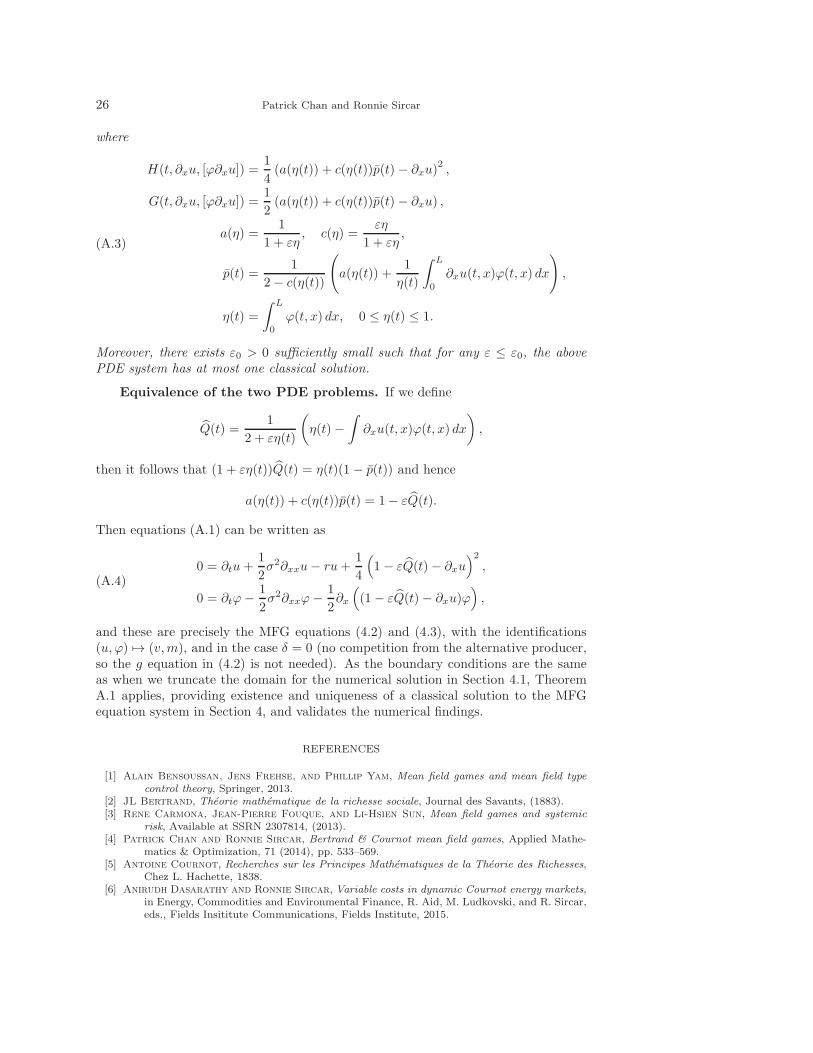
5.3. Numerical illustration. Figure 7 illustrates the numerical solution forthe sustainable economy (5.4). We observe in Figure 7a that while the productionrate q∗ is monotone increasing in x, the exploration level a∗ is monotone decreasing.Figures 7b, 7c and 7d show the sample path for the evolution of the game solution overtime. The system state is described by (Xt) in the top right panel which drives thefeedback controls q∗(Xt) and a∗(Xt) in the bottom panels. One can readily observethat higher reserves lower exploration rates and increase production. The recurrentbehavior of (Xt) is apparent, as the resource is repeatedly exhausted until a newdiscovery replenishes reserves and allows to restart production.

6. Conclusion. In this paper, we apply the Cournot mean field game model tothe global energy market. We focus on the interaction between traditional oil produc-ers and alternative sources (e.g. solar, hydroelectric power, or fracking). Specifically,we investigate the issue from three perspectives: competition, transition, and explo-ration. This leads to three extensions of the basic Cournot MFG model.Transition As the traditional oil producers run out of reserves, they can transition

to energy production with alternative sources. This essentially introduce aNeumann boundary condition to our PDE problem. In the regime of smallexhaustibility, we find explicit correction to the value function and optimalproduction rate by solving a partial integro-differential equation.

Competition We find that if the alternative energy source has a high enough costof production, the traditional energy producers may strategically increaseproduction rate (and hence lowering the energy price ever further) to keepthe alternative energy producer blockaded. This explains OPEC’s strategicdecision not to reduce production quotas in the face of falling oil prices duein large part to the US fracking boom.

Exploration We have studied the impact of exploration and discovery in Cournotmodels of exhaustible resources. We characterize a sustainable energy marketas a stationary solution to the forward Kolmogorov equation. We find thathigher reserves lower exploration rates and increase production.

Appendix A. Existence and Uniqueness. We demonstrate existence anduniqueness of the PDE system (4.2) and (4.3) in the case δ = 0 thanks to the remark-able results by Graber and Bensoussan [9], which were motivated by our prior paper


�*(✁)

✂*(✁)

✄ ☎ ✆ ✝ ✞ ✟ ✠

✄✡☎

✄✡✆

✄✡✝

✄✡✞

(a) Reserves trajectory (b) Production rates

(c) Exploration effort (d) Instantaneous profit

Fig. 7: Trajectory of the game solution over time. Top panel: reserves (Xt) of arepresentative player; middle panel: production rate q∗(Xt); bottom panel: explo-ration rate a∗(Xt). The parameters are δ = 1, λ = 1, r = 0.1, C(a) = 0.1a+ a2/2 andε = 0.25.

[4] on mean field games of Bertrand-type. We first state their thorem, and then showhow the Bertrand problem can be transformed to the Cournot system that we studyin Section 4.

Theorem A.1 (Graber and Bensoussan). Assuming the following on the data:1. uT (x) and m0(x) are functions in C2+γ([0, L]) for some γ > 0;2. uT and m0 satisfy compatible boundary conditions: uT (0) = u′

T (L) = 0 andm0(0) = m0(L) = m′

0(L) = 0;

3. m0 ≥ 0 and∫ L

0 m0(x) dx = 1, i.e. m0 is a probability density;4. uT ≥ 0 and u′

T ≥ 0, i.e. uT is non-negative and non-decreasing.Then there exists a classical solution to the system

∂tu+1

2σ2∂xxu− ru +H(t, ∂xu, [ϕ∂xu]) = 0, 0 < t < T, 0 < x < L,

∂tϕ−1

2σ2∂xxϕ− ∂x (G(t, ∂xu, [ϕ∂xu])ϕ) = 0, 0 < t < T, 0 < x < L,

(A.1)

subject to boundary conditions

ϕ(0, x) = ϕ0(x), u(T, x) = uT (x), 0 ≤ x ≤ L,

u(t, 0) = ϕ(t, 0) = 0, ∂xu(t, L) = 0, 0 ≤ t ≤ T,

1

2σ2∂xϕ(t, L) +G(t, ∂xu(t, L), [ϕ∂xu])ϕ(t, L) = 0, 0 ≤ t ≤ T,

(A.2)


where

H(t, ∂xu, [ϕ∂xu]) =1

4(a(η(t)) + c(η(t))p(t)− ∂xu)

2,

G(t, ∂xu, [ϕ∂xu]) =1

2(a(η(t)) + c(η(t))p(t)− ∂xu) ,

a(η) =1

1 + εη, c(η) =

εη

1 + εη,

p(t) =1

2− c(η(t))

(a(η(t)) +

1

η(t)

∫ L

0

∂xu(t, x)ϕ(t, x) dx

),

η(t) =

∫ L

0

ϕ(t, x) dx, 0 ≤ η(t) ≤ 1.

(A.3)

Moreover, there exists ε0 > 0 sufficiently small such that for any ε ≤ ε0, the abovePDE system has at most one classical solution.

Equivalence of the two PDE problems. If we define

Q(t) =1

2 + εη(t)

(η(t)−

∫∂xu(t, x)ϕ(t, x) dx

),

then it follows that (1 + εη(t))Q(t) = η(t)(1 − p(t)) and hence

a(η(t)) + c(η(t))p(t) = 1− εQ(t).

Then equations (A.1) can be written as

0 = ∂tu+1

2σ2∂xxu− ru+

1

4

(1− εQ(t)− ∂xu

)2,

0 = ∂tϕ−1

2σ2∂xxϕ−

1

2∂x

((1− εQ(t)− ∂xu)ϕ

),

(A.4)

and these are precisely the MFG equations (4.2) and (4.3), with the identifications(u, ϕ) 7→ (v,m), and in the case δ = 0 (no competition from the alternative producer,so the g equation in (4.2) is not needed). As the boundary conditions are the sameas when we truncate the domain for the numerical solution in Section 4.1, TheoremA.1 applies, providing existence and uniqueness of a classical solution to the MFGequation system in Section 4, and validates the numerical findings.

REFERENCES

[1] Alain Bensoussan, Jens Frehse, and Phillip Yam, Mean field games and mean field type

control theory, Springer, 2013.[2] JL Bertrand, Theorie mathematique de la richesse sociale, Journal des Savants, (1883).[3] Rene Carmona, Jean-Pierre Fouque, and Li-Hsien Sun, Mean field games and systemic

risk, Available at SSRN 2307814, (2013).[4] Patrick Chan and Ronnie Sircar, Bertrand & Cournot mean field games, Applied Mathe-

matics & Optimization, 71 (2014), pp. 533–569.[5] Antoine Cournot, Recherches sur les Principes Mathematiques de la Theorie des Richesses,

Chez L. Hachette, 1838.[6] Anirudh Dasarathy and Ronnie Sircar, Variable costs in dynamic Cournot energy markets,

in Energy, Commodities and Environmental Finance, R. Aid, M. Ludkovski, and R. Sircar,eds., Fields Insititute Communications, Fields Institute, 2015.


[7] Sudhakar D Deshmukh and Stanley R Pliska, Optimal consumption and exploration of

nonrenewable resources under uncertainty, Econometrica, (1980), pp. 177–200.[8] Engelbert Dockner, Differential games in economics and management science, Cambridge

University Press, 2000.[9] P Jameson Graber and Alain Bensoussan, Existence and uniqueness of solutions for

Bertrand and Cournot mean field games, arXiv preprint arXiv:1508.05408, (2015).[10] Olivier Gueant, Mean field games and applications to economics, PhD thesis, PhD thesis,

Universite Paris-Dauphine, 2009.[11] Olivier Gueant, Jean-Michel Lasry, and Pierre-Louis Lions, Mean field games and ap-

plications, in Paris-Princeton Lectures on Mathematical Finance 2010, Springer, 2011,pp. 205–266.

[12] Chris Harris, Sam Howison, and Ronnie Sircar, Games with exhaustible resources, SIAMJournal on Applied Mathematics, 70 (2010), pp. 2556–2581.

[13] H. Hotelling, The economics of exhaustible resources, The Journal of Political Economy, 39(1931), pp. 137–175.

[14] Minyi Huang, Peter E Caines, and Roland P Malhame, Individual and mass behaviour

in large population stochastic wireless power control problems: centralized and nash equi-

librium solutions, in Decision and Control, 2003. Proceedings. 42nd IEEE Conference on,vol. 1, IEEE, 2003, pp. 98–103.

[15] Minyi Huang, Roland P Malhame, Peter E Caines, et al., Large population stochastic

dynamic games: closed-loop McKean-Vlasov systems and the Nash certainty equivalence

principle, Communications in Information & Systems, 6 (2006), pp. 221–252.[16] Sebastian Jaimungal and Mojtaba Nourian, Mean-field game strategies for a major-minor

agent optimal execution problem, Available at SSRN 2578733, (2015).[17] Jean-Michel Lasry and Pierre-Louis Lions, Mean field games, Japanese Journal of Math-

ematics, 2 (2007), pp. 229–260.[18] Andrew Ledvina and Ronnie Sircar, Dynamic Bertrand oligopoly, Applied Mathematics &

Optimization, 63 (2011), pp. 11–44.[19] , Oligopoly games under asymmetric costs and an application to energy production,

Mathematics and Financial Economics, 6 (2012), pp. 261–293.[20] Robert E Lucas and Benjamin Moll, Knowledge growth and the allocation of time, tech.

report, National Bureau of Economic Research, 2011.[21] Michael Ludkovski and Ronnie Sircar, Exploration and exhaustibility in dynamic Cournot

games, European Journal of Applied Mathematics, 23 (2012), pp. 343–372.[22] , Game theoretic models for energy production, in Energy, Commodities and Environmen-

tal Finance, R. Aid, M. Ludkovski, and R. Sircar, eds., Fields Insititute Communications,Fields Institute, 2015.

[23] , Technology ladders and R&D in dynamic Cournot markets, J. Economic Dynamics &Control, (2016). To appear.

[24] Michael Ludkovski and Xuwei Yang, Dynamic Cournot models for production of exhaustible

commodities under stochastic demand, in Energy, Commodities and Environmental Fi-nance, R. Aid, M. Ludkovski, and R. Sircar, eds., Fields Insititute Communications, FieldsInstitute, 2015.

[25] Robert S Pindyck, The optimal exploration and production of nonrenewable resources, TheJournal of Political Economy, (1978), pp. 841–861.

fracking, renewables & mean field gameshow opec sets production. the organization of petroleum...

Documents