arX

iv:1

303.

5329

v2 [

mat

h-ph

] 2

Mar

201

4

Forward-Backward Stochastic Differential Systems Associated to

Navier-Stokes Equations in the Whole Space ∗

Freddy Delbaen Jinniao Qiu Shanjian Tang

March 6, 2018

Abstract

A coupled forward-backward stochastic differential system (FBSDS) is formulated in spaces of

fields for the incompressible Navier-Stokes equation in the whole space. It is shown to have a unique

local solution, and further if either the Reynolds number is small or the dimension of the forward

stochastic differential equation is equal to two, it can be shown to have a unique global solution. These

results are shown with probabilistic arguments to imply the known existence and uniqueness results for

the Navier-Stokes equation, and thus provide probabilistic formulas to the latter. Related results and

the maximum principle are also addressed for partial differential equations (PDEs) of Burgers’ type.

Moreover, from truncating the time interval of the above FBSDS, approximate solution is derived for

the Navier-Stokes equation by a new class of FBSDSs and their associated PDEs; our probabilistic

formula is also bridged to the probabilistic Lagrangian representations for the velocity field, given by

Constantin and Iyer (Commun. Pure Appl. Math. 61: 330–345, 2008) and Zhang (Probab. Theory

Relat. Fields 148: 305–332, 2010) ; finally, the solution of the Navier-Stokes equation is shown to be

a critical point of controlled forward-backward stochastic differential equations.

Keywords: forward-backward stochastic differential system, Navier-Stokes equation, Feynman-Kac for-

mula, strong solution, Lagrangian approach, variational formulation.

1 Introduction

Consider the following Cauchy problem for deterministic backward Navier-Stokes equation for the velocity

field of an incompressible, viscous fluid:

∂tu+

ν

2∆u+ (u · ∇)u+∇p+ f = 0, t ≤ T ;

∇ · u = 0, u(T ) = G,(1.1)

which is obtained from the classical Navier-Stokes equation via the time-reversing transformation

(u, p, f)(t, x) 7−→ (−u, p, f)(T − t, x), for t ≤ T.

Here, T > 0, u is the d-dimensional velocity field of the fluid, p is the pressure field, ν ∈ (0,∞) is the

kinematic viscosity, and f is the external force field which, without any loss of generality, is taken to

be divergence free. It is well-known that the Navier-Stokes equation was introduced by Navier [36] and

Stokes [49] via adding a dissipative term ν∆u as the friction force to Euler’s equation, which is Newton’s

law for an infinitesimal volume element of the fluid.∗This research is supported by the Natural Science Foundation of China (Grants #10325101 and #11171076), the Science

Foundation for Ministry of Education of China (No.20090071110001), and the Chang Jiang Scholars Programme. Part of

the work was done when the second author visited Department of Mathematics, ETH, Zurich in the summer of 2011. The

hospitality of ETH is greatly appreciated. He also would like to thank Professors Michael Struwe and Alain-Sol Sznitman

for very helpful discussions and comments related to Navier-Stokes equations. E-mail : delbaen@math.ethz.ch (Freddy

Delbaen), qiujinn@gmail.com (Jinniao Qiu), sjtang@fudan.edu.cn (Shanjian Tang).

1

Forward-backward stochastic differential equations (FBSDEs) are already well-known nowadays to

be connected to systems of nonlinear parabolic partial differential equations (PDEs) (see among many

others [2, 10, 17, 29, 34, 40, 41, 50, 56]). Within such a theory, the d-dimensional Burgers’ equation (in

the backward form) ∂tv +

ν2∆v + (v · ∇)v + f = 0, t ≤ T ;

v(T ) = φ,(1.2)

as a simplified version of Naview-Stokes equation (1.1), is associated in a straightforward way to the

following coupled FBSDE:

dXs(t, x) = Ys(t, x) ds+√ν dWs, s ∈ [t, T ];

Xt(t, x) = x;

−dYs(t, x) = f(s,Xs(t, x)) ds −√νZs(t, x) dWs;

YT (t, x) = G(XT (t, x)).

(1.3)

They are related to each other by the following:

Ys(t, x) = v(s,Xs(t, x)), Zs(t, x) = ∇v(s,Xs(t, x)), s ∈ [t, T ]× Rd (1.4)

and (see [50])

Ys(t,X−1s (t, x)) = v(s, x), Zs(t,X

−1s (t, x)) = ∇v(s, x), s ∈ [t, T ]× Rd (1.5)

with X−1· (t, x) being the inverse of the homeomorphism X·(t, x), x ∈ Rd.

It is a tradition to represent solutions of PDEs as the expected functionals of stochastic processes. The

history is long and the literature is huge. Many studies have been devoted to probabilistic representation

to solution of Navier-Stokes equation (1.1), with the following three methodologies. The first is the

vortex method, which aims to give a probabilistic representation first for the vorticity field, and then

for the velocity field via the Biot-Savart law (which associates the vorticity field directly to the velocity

field, see [35, pages 71-73]). In the two-dimensional case (d = 2), the vorticity turns out to obey

a Fokker-Planck type parabolic PDE, and its probabilistic interpretation is straightforward. In this

line, see Chorin [11] who used random walks and a particle limit to represent the vorticity field, and

Busnello [8] who used the Girsanov transformation to give a probabilistic representation of the vorticity

field, and used the Bismut-Elworthy-Li formula to derive a probabilistic interpretation for the Biot-

Savart law. In the three-dimensional case (d = 3), the vorticity field is still found to evolve as a parabolic

PDE, but it is complicated by the addition of the stretching term; Esposito et al. [24, 23] proposed

a probabilistic representation formula for the vorticity field and then for the velocity field without any

further probabilistic representation for the Biot-Savart law. Busnello et al. [9] used the Bismut-Elworthy-

Li formula to give a probabilistic interpretation for the Biot-Savart law and then for the velocity field.

The second is the Fourier transformation method. Le Jan and Sznitman [31] interpreted the Fourier

transformation of the Laplacian of the three-dimensional velocity field in terms of a backward branching

process and a composition rule along the associated tree, and got a new existence theorem, and their

approach was extensively studied and generalized by others (see, for instance [6, 38]). The third is the

Lagrangian flows method, and see Constantin and Iyer [13] and Zhang [57].

Navier-Stokes equation (1.1) typically has a divergence-free constraint and contains a pressure poten-

tial to complement the thus-lost degree of freedom. Since the pressure in equation (1.1) turns out to be

determined by the Poisson equation (as a consequence of the incompressibility):

∆p = −div div (u⊗ u),

the Navier-Stokes equations (1.1) has the following equivalent form:

∂tu+ ν

2∆u+ (u · ∇)u +∇(−∆)−1div div (u⊗ u) + f = 0, t ≤ T ;

u(T ) = G.(1.6)

2

In comparison with Burgers’ equation (1.2), it has an extra nonlocal operator appearing in its dynamic

equation. To give a fully probabilistic representation for the Navier-Stokes equations, we have to incor-

porate this additional term. In this paper, we associate the Navier-Stokes equation (1.1) to the following

coupled forward-backward stochastic differential system (FBSDS):

dXs(t, x) = Ys(t, x) ds +√ν dWs, s ∈ [t, T ];

Xt(t, x) = x;

−dYs(t, x) =[f(s,Xs(t, x)) + Y0(s,Xs(t, x))

]ds−

√νZs(t, x) dWs;

YT (t, x) = G(XT (t, x));

−dYs(t, x) =d∑

i,j=1

27

2s3Y it Y

jt (t, x +Bs)

(Bi

2s3−Bi

s3

)(Bj

s −Bj2s3

)B s

3ds

− Zs(t, x)dBs, s ∈ (0,∞);

Y∞(t, x) = 0.

(1.7)

Here, B andW are two independent d-dimensional standard Brownian motions, Y and Y satisfy backward

stochastic differential equations and X satisfies a forward one. The forward SDE describes a stochastic

particle system, and the BSDE in the finite time interval specifies the evolution of the velocity. The

drift part of Ys(t, x), s ∈ [t, T ] (see the third equality of FBSDS (1.7)) at time s depends on Y0, and

that of Ys(t, x), s ∈ (0,∞) depends on Yt(t, x + Bs), which make our system (1.7) differ from the

conventional coupled forward-backward stochastic differential equations (FBSDEs) (see [2, 29, 34, 40, 43,

41, 56]). Furthermore, a BSDE in the infinite time interval is introduced to express the integral operator

∇(−∆)−1div div in a probabilistic manner, and both backward stochastic differential equations (BSDEs)

in FBSDS (1.7) are defined on two different time-horizons [t, T ] and (0,∞).

We have

Theorem 1.1. Let G ∈ Hmσ , and f ∈ L2(0, T ;Hm−1

σ ) with m > d/2. Then there is T0 < T which

depends on ‖f‖L2(0,T ;Hm−1), ν, m, d, T and ‖G‖m, such that FBSDS (1.7) admits a unique Hm-solution

(X,Y, Z, Y0) on (T0, T ]. For the solution, there hold the following representations

Zt(t, ·) = ∇Yt(t, ·), Ys(t, ·) = Ys(s,Xs(t, ·)) and Zs(t, ·) := Zs(s,Xs(t, ·)), (1.8)

for T0 < t ≤ s ≤ T . Moreover, there exists some scalar-valued function p such that ∇p = Y0, and (u, p)

with u(t, x) := Yt(t, x) coincides with the unique strong solution to the Navier-Stokes equation (1.1).

In the last theorem, all unknown forward and backward states of the concerned FBSDS evolve in

spaces of fields, and the conditions on f and G are much weaker than those of the existing related results

on coupled FBSDEs (see [2, 17, 29, 34, 41, 45, 56])—which usually require that f and G are either

bounded or uniformly Lipschitz continuous in the space variable x. Related results and the maximum

principle for PDEs of Burgers’ type are also presented in this paper.

FBSDS (1.7) is a complicated version of FBSDE (1.3), including an additional nonlinear and nonlocal

term in the drift of the BSDE to keep the backward state living in the divergence-free subspace. While

the additional term causes difficulty in formulating probabilistic representations, it helps us to obtain the

global solutions if either the Reynolds number is small or the dimension is equal to two.

Our relationship between FBSDS (1.7) and Navier-Stokes equation (1.1) is shown to imply a prob-

abilistic Lagrangian representation for the velocity field, which coincides with the formulas given by

[13, 14, 57] and weakens the regularity assumptions required in the references (see Remark 7.1 below).

On the other hand, in the spirit of the variational interpretations for Euler equations by Arnold [3], Ebin

and Marsden [21] and Bloch et al. [7], Inoue and Funaki [30], Yasue [55] and Gomes [28] formulated

different stochastic variational principles for the Navier-Stokes equations. Along this direction, we give

a new stochastic variational formulation for the Navier-Stokes equations on basis of our probabilistic

Lagrangian representation.

3

Other quite related works include Albeverio and Belopolskaya [1] who constructed a weak solution of

the 3D Navier-Stokes equation by solving the associated stochastic system with the approach of stochastic

flows, Cruzeiro and Shamarova [15] who established a connection between the strong solution to the

spatially periodic Navier-Stokes equations and a solution to a system of FBSDEs on the group of volume-

preserving diffeomorphisms of a flat torus, and Qiu, Tang and You [46] who considered a similar non-

Markovian FBSDS to ours (1.7) in the two-dimensional spatially periodic case, and studied the well-

posedness of the corresponding backward stochastic PDEs.

The rest of this paper is organized as follows. In Section 2, we introduce notations and functional

spaces, and give auxiliary results. In Section 3, the solution to FBSDS (1.7) is defined in suitable spaces

of fields, and our main result (Theorem 3.1) is stated on the FBSDS associated to the Navier-Stokes

Equation. In Section 4, we discuss the coupled FBSDEs for PDEs of Burgers’ type, and related results

and the maximum principle are presented. In Section 5, Theorem 3.1 is proved, and the global existence

and uniqueness of the solution is given if either the Reynolds number is small or the dimension of the

forward SDE is equal to two. By truncating the time interval of the FBSDS, we approximate in Section 6

the Navier-Stokes equation by a class of FBSDSs and associated PDEs. In Section 7, from our relationship

between FBSDS and the Navier-Stokes equation, we derive a probabilistic Lagrangian representation for

the velocity field, which is shown to imply those of [13, 57], and we also give a variational characterization

of the the Navier-Stokes equation. Finally in Section 8 as an appendix, we prove Lemmas 2.2 and 4.1.

2 Preliminaries

2.1 Notations

Let (Ω, F , Ftt≥0,P) be a complete filtered probability space on which are defined two independent

d-dimensional standard Brownian motions W = Wt : t ∈ [0,∞) and B = Bt : t ∈ [0,∞) such that

Ftt≥0 is the natural filtration generated by W and B, and augmented by all the P-null sets in F . By

Ft≥0 and FBt≥0, we denote the natural filtration generated by W and B respectively, and they are

both augmented by all the P-null sets. P is the σ-algebra of the predictable sets on Ω× [0, T ] associated

with Ftt≥0.

The set of all the integers is denoted by Z, with Z+ the subset of the positive elements and N :=

Z+∪0. Denote by |·| (respectively, 〈·, ·〉 or ·) the norm (respectively, scalar product) in finite-dimensional

Hilbert space such as R,Rk,Rk×l, k, l ∈ Z+ and

|x| :=(

k∑

i=1

x2i

)1/2

and |y| :=

k∑

i=1

l∑

j=1

y2ij

1/2

for (x, y) ∈ Rk × Rk×l.

For each Banach space (X , ‖ · ‖X) and real q ∈ [1,∞], we denote by Sq([t, τ ];X ) the set of X -valued,

Ft-adapted and cadlag processes Xss∈[t,τ ] such that

‖X‖Sq([t,τ ];X ) :=

E[sups∈[t,τ ] ‖Xs‖qX

]1/q<∞, q ∈ [1,∞);

ess supω∈Ω sups∈[t,τ ] ‖Xs‖X <∞, q = ∞.

LqF(t, τ ;X ) denotes the set of (equivalent classes of) X -valued predictable processes Xss∈[t,τ ] such that

‖X‖Lq

F(t,τ ;X ) :=

E[ ∫ τ

t ‖Xs‖qX ds]1/q

<∞, q ∈ [1,∞);

ess sup(ω,s)∈Ω×[t,τ ] ‖Xs‖X <∞, q = ∞.

Both(Sq([t, τ ];X ), ‖ · ‖Sq([t,τ ]X )

)and

(Lq

F(t, τ ;X ), ‖ · ‖Lq

F(t,τ ;X )

)are Banach spaces.

Define the set of multi-indices

A := α = (α1, · · · , αd) : α1, · · · , αd are nonnegative integers.

4

For any α ∈ A and x = (x1, · · · , xd) ∈ Rd, denote

|α| =d∑

i=1

αi, xα := xα1

1 xα22 · · ·xαd

d , Dα :=∂|α|

∂xα11 ∂xα2

2 · · ·∂xαd

d

.

For differentiable transformations φ, ψ on Rd, define the Jacobi matrix ∇φ of φ:

∇φ =

∂x1φ1, ∂x2φ

1, · · · , ∂xdφ1

∂x1φ2, ∂x2φ

2, · · · , ∂xdφ2

· · · , · · · , · · · , · · ·∂x1φ

d, ∂x2φd, · · · , ∂xd

φd

whose transpose is denoted by ∇T φ, the divergence divφ = ∇ · φ, and the matrix

φ⊗ ψ =

φ1ψ1, φ1ψ2, · · · , φ1ψd

φ2ψ1, φ2ψ2, · · · , φ2ψd

· · · , · · · , · · · , · · ·φdψ1, φdψ2, · · · , φdψd

.

Now we extend several spaces of real-valued functions to those of vector-valued functions. For l, k ∈Z+, we denote by C∞

c (Rl;Rk) the set of all infinitely differentiable Rk-valued functions with compact

supports on Rl and by D ′(Rl;Rk) the totality of all the Rk-valued general functions with each component

being Schwartz distribution. For simplicity, we write C∞c and D ′ for the case l = k = d. On Rd we denote

by S (S ′, respectively) the set of all the Rd-valued functions whose elements are Schwartz functions

(tempered distributions, respectively). Then the Fourier transform F(f) of f ∈ S is given by

F(f)(ξ) = (2π)−d/2

∫

Rd

exp(−√−1〈x, ξ〉

)f(x) dx, ξ ∈ Rd,

and the inverse Fourier transform F−1(f) is given by

F−1(f)(x) = (2π)−d/2

∫

Rd

exp(√

−1〈x, ξ〉)f(ξ) dξ, x ∈ Rd.

Extended to the general function space S ′, the Fourier transform defines an isomorphism from S ′ onto

itself. As usual, for each s ∈ R and f ∈ S ′, we denote the Bessel potential Is(f) := (1 − ∆)s/2f =

F−1((1 + |ξ|2)s/2F(f)(ξ)).

For l ∈ Z+, m ∈ N, q ∈ [1,∞) and s ∈ [1,∞], by Ls(Rl) and Hm,q(Rl) (Ls and Hm,q, with a little

notional abuse), we denote the usual Rl-valued Lebesgue and Sobolev spaces on Rd, respectively. Hm,q

is equipped with the norm:

‖φ‖m,q :=

(‖φ‖qLq +

m∑

|α|=1

‖Dαφ‖qLq

)1/q

, φ ∈ Hm,q,

which is equivalent to the norm:

‖φ‖m,q := ‖(1−∆)m2 φ‖Lq , φ ∈ Hm,q, for q ∈ (1,∞).

Both norms will not be distinguished unless there is a confusion. In particular, for the case of q = 2,

Hm,2 is a Hilbert space with the inner product:

〈φ, ψ〉m :=

∫

Rd

〈Im/2φ(x), Im/2ψ(x)〉 dx, φ, ψ ∈ Hm,2.

5

We define the duality between Hs,q and Hr,q′ for q ∈ (1,∞) and q′ = q/(q − 1) as:

〈φ, ψ〉s,r :=

∫

Rd

〈Is/2φ(x), Ir/2ψ(x)〉 dx, φ ∈ Hs,q, ψ ∈ Hr,q′ .

For simplicity, we write the space Hm and the norm ‖ · ‖m for Hm,2 and ‖ · ‖m,2, respectively.

Define

Dσ := φ ∈ C∞c : ∇ · φ = 0 .

Denote by Hm,qσ the completion of Dσ under the norm ‖ · ‖m,q, which is a complete subspace of Hm,q.

Now we introduce several spaces of continuous functions. For l ∈ Z+, k ∈ N and domain O ⊂ Rd, we

denote by C(O,Rl), Ck(O,Rl) and Ck,δ(O,Rl) with δ ∈ (0, 1) the continuous function spaces equipped

with the following norms respectively:

‖φ‖C(O,Rl) := supx∈O

|φ(x)|, ‖φ‖Ck(O,Rl) := ‖φ‖C(O,Rl) +

k∑

|α|=1

‖Dαφ‖C(O,Rl),

‖φ‖Ck,δ(O,Rl) := ‖φ‖Ck(O,Rl) +∑

|α|=k

supx,y∈O,x 6=y

|Dαφ(x) −Dαφ(y)||x− y|δ ,

with the convention that C0(O,Rl) ≡ C(O,Rl). Whenever there is no confusion, we write C(Rd), Ck,

and Ck,δ for C(Rd,Rl), Ck(Rd,Rl) and Ck,δ(Rd,Rl), respectively.

In an obvious way, we define spaces of Banach space valued functions such as C(0, T ;Hm,q) and

Lr(0, T ;Hm,q) for m ∈ Z, r, q ∈ (1,∞), and related local spaces like the following ones:

Lrloc(T0, T ;H

m,q) : =⋂

T1∈(T0,T ]

Lr(T1, T ;Hm,q),

Cloc((T0, T ];Hm,q) : =

⋂

T1∈(T0,T ]

C([T1, T ];Hm,q).

2.2 Auxiliary results

In the remaining part of the work, we shall use C to denote a constant whose value may vary from line to

line, and when needed, a bracket will follow immediately after C to indicate what parameters C depends

on. By A → B we mean that normed space (A, ‖ · ‖A) is embedded into (B, ‖ · ‖B) with a constant C

such that

‖f‖B ≤ C‖f‖A, ∀f ∈ A.

Lemma 2.1. There holds the following assertions:

(i) For integer n > d/q + k with k ∈ N and q ∈ (1,∞), we have Hn,q → Ck,δ , for any δ ∈(0, (n− d/q − k) ∧ 1).

(ii) If 1 < r < s <∞ and m,n ∈ N such that ds −m = d

r − n, then Hn,r → Hm,s.

(iii) For any s > d/2, Hs is a Banach algebra, i.e., there is a constant C > 0 such that,

‖φψ‖s ≤ C‖φ‖s‖ψ‖s, ∀φ, ψ ∈ Hs.

The first two assertions are borrowed from the well-known embedding theorem in Sobolev space

(see [53]), and the last one is referred to [35, Lemma 3.4, Page 98].

Remark 2.1. Note that d = 2 or 3 throughout this work. For any h, g ∈ H2, we have

‖h · g‖21

= ‖h · g‖20 +d∑

i=1

‖∂xih · g‖20 +

d∑

i=1

‖h · ∂xig‖20

6

≤C‖h‖2C(Rd)‖g‖20 + ‖∇h‖2β0 ‖∇h‖2−2β

1 ‖g‖2β0 ‖g‖2−2β1 + ‖h‖2C(Rd)‖g‖21

(using Gagliardo-Nirenberg Inequality (see [26, 33, 37])

)

≤C‖h‖22‖g‖21,

where β := 1 − d/4, and H2 → C0,δ for some δ ∈ (0, 1). In view of Lemma 2.1, we have for any integer

m > d/2,

‖hg‖m−1 ≤ C(m, d)‖h‖m‖g‖m−1, ∀h ∈ Hm, g ∈ Hm−1.

Next, we discuss the the composition of generalized functionals with stochastic flows with Sobolev

space-valued coefficients. Assume that ν > 0 and that

b ∈ C([0, T ];Hm) ∩ L2(0, T ;Hm+1), φ ∈ L2(0, T ;L2(Rd)), ψ ∈ L2(Rd), (2.1)

for some integer m > d/2. Consider the following FBSDE:

dXs(t, x) = b(s,Xs(t, x)) ds+√ν dWs, s ∈ [t, T ];

Xt(t, x) = x;

−dYs(t, x) = φ(s,Xs(t, x)) ds−√νZs(t, x) dWs, s ∈ [t, T ];

YT (t, x) = ψ(XT (t, x)).

(2.2)

Since Hm → C0,δ and Hm+1 → C1,δ for m > d/2, in view of [32, Theorems 3.4.1 and 4.5.1], the forward

SDE is well posed for each (t, x) ∈ [0, T ] × Rd, and the unique solution in relevance to the initial data

(t, x) ∈ [0, T ]×Rd defines a stochastic flow of homeomorphisms. Since the function φ is only measurable,

the following lemma serves to justify the composition φ(s,Xs(t, x)).

Lemma 2.2. Assume that m > d/2 and b ∈ C([0, T ];Hm) ∩L2(0, T ;Hm+1). Then for all t ∈ [0, T ], s ∈[t, T ], (ϕ, η) ∈ L1(Rl)× L1([0, T ]× Rd;Rl), l ∈ Z+, we have

κ‖ϕ‖L1(Rl) ≤∫

Rd

E[|ϕ(Xs(t, x))|

]dx ≤ κ−1‖ϕ‖L1(Rl), (2.3)

λ‖η‖L1([t,T ]×Rl) ≤∫

Rd

∫ T

t

E[|η(s,Xs(t, x))|

]dsdx ≤ λ−1‖η‖L1([t,T ]×Rl), (2.4)

with κ = e−‖div b‖L1(t,s;L∞) and λ = e−‖div b‖L1(t,T ;L∞) .

Lemma 2.2 weakens the assumptions on b of [4, Theorem 14.3], where b(t, ·) ≡ b(·) is time invariant

and is required to lie in C1(Rd) ∩ L2(Rd). Since b(t, x) is not necessarily uniformly Lipschitz continuous

in x, the stability of X with respect to the coefficient b has to be proved very carefully and the proof of

[4, Theorem 14.3] has to be generalized accordingly. We give a probabilistic proof in the appendix.

Remark 2.2. From Lemma 2.2, we see that Lebesgue’s measure transported by the flow Xs(t, x), s ∈[t, T ] results in a group of measures µs, s ∈ [t, T ] satisfying for any Borel measurable set A ⊂ Rd,

µs(A) =

∫

Rd

E [1A(Xs(t, x))] dx.

These measures are all equivalent to Lebesgue measure and the exponential rate of compression or dilation

are governed by the divergence of b. In particular, when b is divergence free,Xs(t, ·) preserves the Lebesguemeasure for all times. This is similar to that of a system of ordinary differential equations (see [20]). On

the other hand, thanks to Lemma 2.2, our FBSDE (2.2) makes sense under assumption (2.1), i.e., the

forward SDE is well posed for each (t, x) ∈ [0, T ]×Rd and for each t ∈ [0, T ] the BSDE is well posed for

almost every x ∈ Rd.

7

3 FBSDS associated with Navier-Stokes Equation

Definition 3.1. Let T0 < T . (X,Y, Z, Y0) is called an Hm-solution to FBSDS (1.7) in [T0, T ] if for

almost every (t, x) ∈ [T0, T ]× Rd,

(X·(t, x), Y·(t, x), Z·(t, x)) ∈ S2([t, T ];Rd)× S2([t, T ];Rd)× L2F (t, T ;Rd×d)

and for each t ∈ [T0, T ] and almost every x ∈ Rd, Ys(t, x), s ∈ [t, T ] ∈ L2(t, T ;L∞(Ω;Rd)), such that

all the stochastic differential equations of (1.7) hold in Ito’s sense and Y0(t, x) := limε↓0 EYε(t, x) exists

for almost every (t, x) ∈ (T0, T ]× Rd with Y0 ∈ L2loc(T0, T ;H

m−1).

Our main result is stated as follows.

Theorem 3.1. Let ν > 0, G ∈ Hmσ , and f ∈ L2(0, T ;Hm−1

σ ) with m > d/2. Then there is T0 < T which

depends on ‖f‖L2(0,T ;Hm−1), ν, m, d, T and ‖G‖m, such that FBSDS (1.7) has a unique Hm-solution

(X,Y, Z, Y0) on (T0, T ] with the function

Yt(t, x), (t, x) ∈ (T0, T ]× Rd ∈ Cloc((T0, T ];Hmσ ) ∩ L2

loc(T0, T ;Hm+1σ ).

Moreover, we have the following representations

Zt(t, ·) = ∇Yt(t, ·), Ys(t, ·) = Ys(s,Xs(t, ·)) and Zs(t, ·) := Zs(s,Xs(t, ·)), (3.1)

for T0 < t ≤ s ≤ T , and there is some scalar-valued function p such that ∇p = Y0 and (Y, Z, p) satisfies

Yr(r,Xr(t, x)) =G(XT (t, x)) +

∫ T

r

[f(s,Xs(t, x)) +∇p(s,Xs(t, x))] ds

−√ν

∫ T

r

Zs(s,Xs(t, x)) dWs, T0 < t ≤ r ≤ T, a.e.x ∈ Rd, a.s., (3.2)

and (u, p) with u(t, x) := Yt(t, x) is the unique strong solution to Navier-Stokes equation (1.1) on (T0, T ].

As indicated in the introduction, Navier-Stokes equation (1.1) is equivalent to (1.6):

∂tu+ ν

2∆u+ (u · ∇)u +∇(−∆)−1div div (u⊗ u) + f = 0, t ≤ T ;

u(T ) = G.

To give a fully probabilistic solution of Navier-Stokes equation (1.1), we shall first give a probabilistic

representation for the nonlocal operator ∇(−∆)−1div div. Note that a different probabilistic formulation

for ∇p = ∇(−∆)−1div div (u⊗ u) was given by Albeverio and Belopolskaya [1] for d = 3.

Lemma 3.2. For φ, ψ ∈ Hm with m > d2 + 1, the following BSDE :

−dYs(x) =27

2s3

d∑

i,j=1

φiψj(x+Bs)(Bj

s − Bj2s3

)(Bi

2s3−Bi

s3

)B s

3ds

− Zs(x)dBs, s ∈ (0,∞);

Y∞(x) = 0

(3.3)

is well-posed on (0,∞) and Y0(x) := limε↓0 EYε(x) exists for each x ∈ Rd. Moreover, Y0 ∈ C(Rd) and

Y0(x) = ∇(−∆)−1div div(φ⊗ ψ)(x) =

d∑

i,j=1

∇(−∆)−1∂xi∂xj (φi(x)ψj(x)), ∀x ∈ Rd.

8

Proof. For m > d/2 + 1, Hm is a Banach algebra embedded into H2,γ for some γ > d and also into

C1,δ(Rd) for some δ ∈ (0, 1). Thus, φiψ ∈ Hm ∩ Hm,1 and ∂xi∂xj (φi(x)ψj(x)) ∈ H0,γ(R) ∩ H0,1(R),

i, j = 1, · · · , d.For each ε > 0,

E

[∫ ∞

ε

27

2s3

∣∣∣φiψj(x+Bs)(Bi

2s3−Bi

s3

)(Bj

s − Bj2s3

)B s

3

∣∣∣ ds]

≤ ‖φiψj‖L∞

∫ ∞

ε

27

2s3E[∣∣∣(Bi

2s3−Bi

s3

)(Bj

s −Bj2s3

)B s

3

∣∣∣]ds

≤ C ‖φ⊗ ψ‖2∫ ∞

ε

1

s3/2ds <∞, i, j = 1, · · · , d.

Thus, BSDE (3.3) is well-posed on [ε,∞].

Note that

Yε(x) = E

∫ ∞

ε

27

2s3

d∑

i,j=1

φiψj(x+Bs)(Bi

2s3−Bi

s3

)(Bj

s −Bj2s3

)B s

3ds∣∣∣FB

ε

.

Applying the integration-by-parts formula, we obtain

E

[27

2s3φiψj(x+Bs)

(Bi

2s3−Bi

s3

)(Bj

s −Bj2s3

)B s

3

]

=27

2s3

∫

Rd

∫

Rd

∫

Rd

φiψj(x+ y + z + r)yizjrk(2πs/3)−3d/2e−3(|y|2+|z|2+|r|2)

2s dydzdr

=− 9

2s2

∫

Rd

∫

Rd

∫

Rd

φiψj(y)zjrk(2πs/3)−3d/2∂yie−3(|y−x−z−r|2+|z|2+|r|2)

2s dydzdr

= · · ·

=1

2s

∫

Rd

∂xi∂xj (φiψj)(y + x)yk(2πs)−d/2e−|y|2

2s dy

=1

2sE[∂xi∂xj (φiψj)(x+ Bs)B

ks

], s > 0, i, j, k = 1, · · · , d.

As for i, j = 1, · · · , d

s−1

∫

Rd

|∂xi∂xj (φiψj)(y + x)y(2πs)−d/2e−|y|2

2s | dy

≤C s−d2−1‖∂xi∂xj (φiψj)‖0,q

√ss

d2 (1−

1q)

≤C ‖∂xi∂xj (φiψj)‖0,qs−12−

d2q , q ∈ [1, γ],

(3.4)

and∫ ∞

0

s−1E[∣∣∂xi∂xj (φiψj)(x+Bs)B

ks

∣∣] ds

=

∫ ∞

0

s−1

∫

Rd

|∂xi∂xj (φiψj)(y + x)yk(2πs)−d/2e−|y|2

2s | dy ds

≤C

∫ 1

0

‖∂xi∂xj (φiψj)‖0,γ s−12−

d2γ ds+ C

∫ ∞

1

‖∂xi∂xj (φiψj)‖0,1 s−d+12 ds

≤C(‖∂xi∂xj (φiψj)‖m−2 + ‖∂xi∂xj (φiψj)‖m−2,1

), (3.5)

we have

limε↓0

E[Y kε (x)

]= lim

ε↓0

∫ ∞

ε

1

2s

∫

Rd

∂xi∂xj (φiψj)(y + x)yk(2πs)−d/2e−|y|2

2s dyds

9

=

∫ ∞

0

1

2s

∫

Rd

∂xi∂xj(φiψj)(y + x)yk(2πs)−d/2e−|y|2

2s dyds

(by (3.5) and Fubini Theorem)

=

∫

Rd

∂xi∂xj (φiψj)(x + y)yk∫ ∞

0

1

2s(2πs)−d/2e−

|y|2

2s dsdy

=Γ(d/2)

2πd/2

∫

Rd

∂xi∂xj (φiψj)(x + y)yk

|y|d dy

= ∂xk(−∆)−1∂xi∂xj (φiψj)(x),

which coincides with the convolution representation of the operator ∇(−∆)−1 described in [35, Page 31].

Hence, BSDE (3.3) are well-posed on (0,∞) and by (3.5), one has Y0 ∈ C(Rd) due to the continuity of

the translation operator on Lp(Rd), p ∈ [1,∞). Moreover, we have

Y0(x) = ∇(−∆)−1∂xi∂xj (φi(x)ψj(x)) = limε↓0

E[Yε(x)

], ∀x ∈ Rd.

The proof is complete.

Remark 3.1. Applying the integration-by-parts formulas in the above proof, we see that BSDE (3.3)

gives a probabilistic representation for the operator∇(−∆)−1div div in the spirit of the Bismut-Elworthy-

Li formula (see [22]). Its generator does not contain any of its own unknowns and is trivial in its form,

while the existence of its solution goes beyond existing results on infinite horizon BSDEs (see [44] and

references therein) as the generator may fail to be integrable on the whole time horizon [0,∞). In fact, the

operator P := I−∇∆−1div is the Leray-Hodge projection onto the space of divergence free vector fields,

where I is the identity operator. Define P⊥ := I−P. We have in Lemma 3.2 that Y0 = −P⊥(div(φ⊗ψ)).Indeed, the singular integral operator P (see [35, 48]) is a bounded transformation in Hn,q for q ∈ (1,∞)

and n ∈ Z. Note that for any g ∈ Hmσ , integration-by-parts formula yields

〈P⊥(div(φ⊗ ψ)), g〉m−2,m = 0.

Remark 3.2. There is a scalar function η such that Y0 = ∇η. It is sufficient to take

η(x) =: (−∆)−1∂xi∂xj (φiψj)(x) ∈ Hm,2(R)

by the theory of second order Elliptic PDEs (see [27]).

Remark 3.3. For any ε > 0, we have by Minkowski inequality

∥∥∥E[Yε

]∥∥∥0=

∥∥∥∥∥∥

d∑

i,j=1

E

[∫ ∞

ε

27

2s3φiψj(·+Bs)

(Bi

2s3−Bi

s3

)(Bj

s −Bj2s3

)B s

3ds

]∥∥∥∥∥∥0

≤d∑

i,j=1

‖φiψj‖0E∫ ∞

ε

27

2s3

∣∣∣(Bi

2s3−Bi

s3

)(Bj

s −Bj2s3

)B s

3

∣∣∣ ds

≤ 27√ε

d∑

i,j=1

‖φiψj‖0. (3.6)

Putting

Pε(φ⊗ ψ) = E[Yε

], ∀φ, ψ ∈ Hm, m > d/2 + 1,

we have

‖Pε(φ ⊗ ψ)‖k ≤ C√ε‖φ⊗ ψ‖k, ∀ 0 ≤ k ≤ m,

with the constant C being independent of ε. Then, the operatorPε can be seen as a regular approximation

of −P⊥div. This approximation will be used to study approximate solution of Navier-Stokes equation in

Section 6.

10

4 FBSDEs for PDEs of Burgers’ type

The PDE of Burgers’ type:

∂tu+ ν

2∆u+((b+ αu) · ∇

)u+ cu+ φ = 0, t ≤ T ;

u(T ) = ψ,(4.1)

is easily connected to the following coupled FBSDE:

dXs(t, x) = [b(s,Xs(t, x)) + αYs(t, x)] ds+√ν dWs, s ∈ [t, T ];

Xt(t, x) = x;

−dYs(t, x) = [φ(s,Xs(t, x)) + c(s,Xs(t, x))Ys(t, x)] ds−√νZs(t, x) dWs, s ∈ [t, T ];

YT (t, x) = ψ(XT (t, x)),

(4.2)

where ν > 0 and α are constants. The classical Burgers’ equation is the case where α = 1, b ≡ 0 and

c ≡ 0.

Definition 4.1. Let T0 < T . We say (X,Y, Z) is a solution to FBSDE (4.2) on [T0, T ] if for each

t ∈ [T0, T ] and almost every x ∈ Rd,

(X·(t, x), Y·(t, x), Z·(t, x)) ∈ S2([t, T ];Rd)× S2([t, T ];Rd)× L2F (t, T ;Rd×d)

and such that the forward SDE and BSDE on [t, T ] hold in Ito’s sense. If for each t ∈ [T0, T ] and almost

every x ∈ Rd, we further have

Y·(t, x) ∈ L2(t, T ;L∞(Ω;Rd)), (4.3)

then (X,Y, Z) is called a strengthened solution.

Lemma 4.1. Let b ∈ C([T0, T ];Hm) ∩ L2(T0, T ;H

m+1), φ ∈ L2(T0, T ;Hm−1), and ψ ∈ Hm, with

m > d/2 and T0 ∈ [0, T ). Then, the following FBSDE:

dXs(t, x) = b(s,Xs(t, x)) ds+√ν dWs, T0 ≤ t ≤ s ≤ T ;

Xt(t, x) = x;

−dYs(t, x) = φ(s,Xs(t, x)) ds−√νZs(t, x) dWs, s ∈ [t, T ];

YT (t, x) = ψ(XT (t, x))

(4.4)

has a unique solution (X,Y, Z) such that the function

Yt(t, x), (t, x) ∈ [T0, T ]× Rd ∈ C([T0, T ];Hm) ∩ L2(T0, T ;H

m+1).

For each t ∈ [T0, T ], almost all x ∈ Rd and all r ∈ [t, T ], we have

Yr(r,Xr(t, x)) = ψ(XT (t, x)) +

∫ T

r

φ(s,Xs(t, x)) ds−√ν

∫ T

r

Zs(s,Xs(t, x)) dWs, a.s., (4.5)

Zt(t, x) = ∇Yt(t, x), (Yr(t, x), Zr(t, x)) = (Yr , Zr)(r,Xr(t, x)), a.s.. (4.6)

Moreover, for any t ∈ [T0, T ]

‖Yt(t)‖2m + ν

∫ T

t

‖Zs(s)‖2m ds = ‖YT (T )‖2m + 2

∫ T

t

〈φ(s) + Zsb(s), Ys(s)〉m−1,m+1 ds. (4.7)

A proof is sketched in the appendix for the reader’s convenience, though it might exist elsewhere.

Proposition 4.2. Assume that ψ ∈ Hm, b ∈ C([0, T ];Hm) ∩ L2(0, T ;Hm+1), c ∈ L2(0, T ;Hm(Rd×d))

and φ ∈ L2(0, T ;Hm−1) with m > d/2. Then there is T0 < T which depends on ‖ψ‖m, ‖b‖C([0,T ];Hm),

11

‖c‖L2(0,T ;Hm), ‖φ‖L2(0,T ;Hm−1), α, ν, m, d and T , such that FBSDE (4.2) has a unique strengthened

solution on (T0, T ] and if α = 0, the existence time interval is [0, T ]. Moreover,

(i) Yt(t, x), (t, x) ∈ (T0, T ]× Rd

∈ Cloc((T0, T ];H

m) ∩ L2loc(T0, T ;H

m+1);

(ii) for almost every x ∈ Rd and all s ∈ [t, T ],

Ys(s,Xs(t, x)) =ψ(XT (t, x)) +

∫ T

s

(φ+ cYr) (r,Xr(t, x)) dr −√ν

∫ T

s

Zr(r,Xr(t, x)) dWr , a.s., (4.8)

Zt(t, x) =∇Yt(t, x), (Ys(t, x), Zs(t, x)) = (Ys, Zs)(s,Xs(t, x)), a.s.; (4.9)

(iii) for any t ∈ (T0, T ], we have the following energy equality:

‖Yt(t)‖2m =‖ψ‖2m + 2

∫ T

t

〈Zs(b+ αYs)(s), Ys(s)〉m−1,m+1 ds

+ 2

∫ T

t

〈c Ys(s) + φ(s), Ys(s)〉m−1,m+1 ds− ν

∫ T

t

‖Zs(s)‖2m ds.

(4.10)

In particular, if m > d/2+1, the strengthened solution on the time interval (T0, T ] is the unique solution

as well.

In addition, Yt(t, x) is the unique strong solution to PDE (4.1) on (T0, T ].

Remark 4.1. When α = 0, b ≡ 0 and c ≡ 0, PDE (4.1) becomes the classical d-dimensional Burgers’

equation. With the method of stochastic flows, Constantin and Iyer [13] and Wang and Zhang [54] give

different stochastic representations for the local regular solutions of Burgers’ equations based on stochastic

Lagrangian paths. Moreover, in Wang and Zhang [54] the global existence results are also presented under

certain assumptions on the coefficients. To focus on the Navier-Stokes equation, we shall not search such

global results for the PDEs of Burgers’ type in this work. Nevertheless, the conditions on the coefficients

herein are much weaker than those in [13, 54] where G and f(t, ·) are continuous in the space variable

and take values in Ck+1,α and Hk+3,q (→ Ck+2) with (k, α, q) ∈ N× (0, 1)× (d∨ 2,∞), respectively. We

also note that Cruzeiro and Shamarova [16] through a forward-backward stochastic system describes a

probabilistic representation of Hn-regular (n > d2 +2) solutions for the spatially periodic forced Burgers’

equations.

Remark 4.2. In Proposition 4.2, we see Yt(t, x) and Zt(t, x) are all deterministic functions on (T0, T ]×Rd.

Therefore, for each semi-martingale X ′s(t, x), s ∈ [t, T ] of the form

X ′s(t, x) = x+

∫ s

t

ϕr(t, x) dr +

∫ s

t

√ν dWr , T0 < t ≤ s ≤ T

with ϕs(t, x), s ∈ [t, T ] being bounded and predictable, it is interesting to understand (Ys, Zs)(s,

X ′s(t, x)) in FBSDE framework. Indeed, define the following equivalent probability measure:

dQt,x

dP:= exp

(1√ν

∫ T

t

[(b + αYs)(s,X

′s(t, x))− ϕs(t, x)

]dWs

− 1

2ν

∫ T

t

|(b+ αYs)(s,X′s(t, x)) − ϕs(t, x)|2 ds

).

Then in view of Girsanov theorem, there is a standard Brownian motion (W ′,Qt,x) such that

X ′s(t, x) = x+

∫ r

t

(b+ αYr)(r,X′r(t, x)) dr +

∫ s

t

√ν dW ′

r, T0 < t ≤ s ≤ T.

Then, we obtain

Yτ (τ,X′τ (t, x)) = ψ(X ′

T (t, x)) +

∫ T

τ

(φ+ c Ys) (s,X′s(t, x)) ds −

√ν

∫ T

τ

Zs(s,X′s(t, x)) dW

′s

12

= ψ(X ′T (t, x)) +

∫ T

τ

[φ+ c Ys + Zs(b+ αYs)

](s,X ′

s(t, x))− Zsϕs(t, x)ds

−√ν

∫ T

τ

Zs(s,X′s(t, x)) dWs.

of Proposition 4.2. Step 1. Existence of the solution. Choose (bn, cn, φn, ψn) ∈ C∞c (R1+d;Rd) ×

C∞c (R1+d;Rd×d)×C∞

c (R1+d;Rd)×C∞c (Rd;Rd) such that, putting (δbn, δcn, δφn, δψ) = (b−bn, c−cn, φ−

φn, ψ − ψn), we have

limn→∞

[‖δbn‖C([0,T ];Hm) + ‖δbn‖L2(0,T ;Hm+1) + ‖δcn‖L2(0,T ;Hm) + ‖δφn‖L2(0,T ;Hm−1) + ‖δψn‖m

]= 0,

‖bn‖C([0,T ];Hm) ≤ C‖b‖C([0,T ];Hm), ‖φn‖L2(0,T ;Hm−1) ≤ C‖φ‖L2(0,T ;Hm−1), ‖ψn‖m ≤ C‖ψ‖m,

‖cn‖L2(0,T ;Hm) ≤ C‖c‖L2(0,T ;Hm), and ‖bn‖L2(0,T ;Hm+1) ≤ C‖b‖L2(0,T ;Hm+1), where C is a universal

constant being independent of n. By the existing FBSDE theory (for instance, see [34]), for each n,

FBSDE (4.2) with (b, c, φ, ψ) being replaced by smooth triple (bn, cn, φn, ψn) admits a local solution

(Xn, Y n, Zn) on some time interval (τ, T ] such that (Y n, Zn) satisfies (4.9). Then we have by Lemma

4.1,

‖Y ns (s)‖2m + ν

∫ T

s

‖Znr (r)‖2m dr

= ‖ψn‖2m +

∫ T

s

2 (〈Znr (bn + αY n

r )(r), Y nr (r)〉m−1,m+1 + 〈(φn(r) + cnY

nr (r), Y n

r (r)〉m−1,m+1) dr

≤C

∫ T

s

(‖(bn + αY n

r )(r)‖m‖Znr (r)‖m−1‖Y n

r (r)‖m+1 + ‖cn(r)‖m‖Yr(r)‖2m + ‖φn(r)‖m−1‖Y nr (r)‖m+1

)dr

+ ‖ψn‖2m

≤ C

∫ T

s

(‖bn(r)‖2m + ‖cn(r)‖m + 1

)‖Y n

r (r)‖2m dr + α2

∫ T

s

‖Y nr (r)‖4m dr +

∫ T

s

‖φ(r)‖2m−1 dr

+ν

2

∫ T

s

‖Znr (r)‖2m dr + C‖ψ‖2m.

Gronwall inequality implies

‖Y ns (s)‖2m + ν

∫ T

s

‖Znr (r)‖2m dr

≤C exp

∫ T

0

(‖bn(r)‖2m + ‖cn(r)‖m + 1

)dr

(‖ψ‖2m + ‖φ‖2L2(0,T ;Hm) + α2

∫ T

s

‖Y nr (r)‖4m dr

)

≤C exp

∫ T

0

C(‖b(r)‖2m + ‖c(r)‖2m + 1

)dr

(‖ψ‖2m + ‖φ‖2L2(0,T ;Hm) + α2

∫ T

s

‖Y nr (r)‖4m dr

)

≤C0

(1 + α2

∫ T

s

‖Y nr (r)‖4m dr

)(4.11)

with the constant C0 depending only on ‖φ‖L2(0,T ;Hm−1), ‖b‖C([0,T ];Hm), ‖c‖L2(0,T ;Hm), ‖ψ‖m, ν, m, d

and T . Hence, applying Gronwall inequality again and setting

τ0 =

(T − 1

|C0α|2)∨ 0,

we have for any s ∈ (τ0, T ],

supr∈[s,T ]

‖Y nr (r)‖2m + ν

∫ T

s

‖Znr (r)‖2m dr ≤ C0

1− |αC0|2(T − s). (4.12)

13

As a consequence, we are allowed to choose a uniform existing time interval (τ, T ] for all (Xn, Y n, Zn),

n ∈ Z+.

Put

(Xnk, Y nk, Znk, bnk, cnk, φnk, ψnk) = (Xn, Y n, Zn, bn, cn, φn, ψn)− (Xk, Y k, Zk, bk, ck, φk, ψk).

Then for each ε ∈ (0, T − τ), we have, for any s ∈ (τ + ε, T ]

‖Y nks (s)‖2m + ν

∫ T

s

‖Znkr (r)‖2m dr

= ‖ψnk‖2m +

∫ T

s

2(〈(Zn

r bnk + Znkr bk + cnkY

nr + ckY

nkr + φnk)(r), Y

nkr (r)〉m−1,m+1

)dr

+

∫ T

s

2α〈Znr Y

nkr (r) + Znk

r Y kr (r), Y nk

r (r)〉m−1,m+1 dr

≤‖ψnk‖2m +ν

2

∫ T

s

(‖Znkr (r)‖2m + ‖Y nk

r (r)‖2m) dr

+ C

α2

∫ T

s

(‖Y nk

r (r)‖2m‖Y nr (r)‖2m + ‖Y nk(r)‖2m‖Y k

r (r)‖2m)dr

+

∫ T

s

(‖φnk‖2m−1 +

(‖bnk‖2m + ‖cnk‖2m)‖Y n

r ‖2m +(‖bk‖2m + ‖ck‖m

)‖Y nk

r ‖2m)(r) dr

≤ ‖ψnk‖2m +

∫ T

s

[ν

2‖Znk

r ‖2m + C(‖bnk‖2m + ‖cnk‖2m + ‖φnk‖2m−1 + (1 + ‖ck‖m)‖Y nk

r ‖2m) ]

(r) dr.

Consequently, for a constant C which is independent of n and k, we have

sups∈[T0+ε,T ]

‖Y nkr (s)‖2m + ν

∫ T

T0+ε

‖Znkr (r)‖2m dr

≤C

‖ψnk‖2m +

∫ T

0

(‖bnk‖2m + ‖cnk‖2m + ‖φnk‖2m−1

)(r) dr

−→ 0 as n, k → ∞.

(4.13)

Then (Y nr (r, x), Zn

r (r, x)), (t, x) ∈ [τ+ε, T ]×Rdn∈Z+ is a Cauchy sequence in C([τ+ε, T ];Hm)×L2(τ+

ε, T ;Hm) for any ε ∈ (0, T − τ), having a limit denoted by (ζ(r, x),∇ζ(r, x)).On the other hand, FBSDE

dXs(t, x) = [b(s,Xs(t, x)) + αζ(s,Xs(t, x))] ds+√ν dWs ;

Xt(t, x) = x;

−dYs(t, x) = (φ+ c ζ)(s,Xs(t, x)) ds−√νZs(t, x) dWs, s ∈ [t, T ];

YT (t, x) = ψ(XT (t, x)),

(4.14)

admits a unique solution (X,Y, Z) on (τ, T ], which by Lemma 4.1 satisfies (4.5) and (4.6). Setting

k → ∞ first and then n→ ∞ in (4.13), we have ζ(t, x) = Yt(t, x) and ∇ζ(t, x) = Zt(t, x) for almost every

(t, x) ∈ (τ, T ]×Rd. Again from Lemma 4.1, we see that the triple (Xs(t, x), ζ(s,Xs(t, x)), ∇ζ(s,Xs(t, x)))

solves FBSDE (4.2) and satisfies all the assertions of this proposition except the uniqueness and the

relation to PDE (4.1), which are left to the next steps. Moreover, through a bootstrap argument, we

can extend the existing interval to a maximal one denoted by (T0, T ] with T0 depending on ‖ψ‖m,

‖b‖C([0,T ];Hm), ‖c‖L2(0,T ;Hm), ‖φ‖L2(0,T ;Hm−1), α, m, d, ν and T . In particular, if α = 0, it follows from

estimates (4.11) and (4.12) that the existence time interval is [0, T ].

Step 2. Uniqueness. First, for m > d/2 + 1, as Hm−1 → C0,δ(Rd) for some δ ∈ (0, 1), our BSDE

is well-posed for each x ∈ Rd. Then Ito’s formula yields that for T0 < t ≤ s ≤ T ,

|Ys(t, x)|2 + E

[ν

∫ T

s

|Zr(t, x)|2dr∣∣∣Fs

]

14

= E

[|ψ(XT (t, x))|2 + 2

∫ T

s

〈Yr(t, x), φ(r,Xr(t, x)) + c(r,Xr(t, x))Yr(t, x)〉 dr∣∣∣Fs

]

≤ C(m, d)

‖ψ‖2m + ‖φ‖2L2(0,T ;Hm−1) +

∫ T

s

(1 + ‖c(r)‖m)E[|Yr(t, x)|2

∣∣Fs

]dr

,

which by Gronwall inequality implies that for each (t, x) ∈ (T0, T ]× Rd, there holds almost surely

|Ys(t, x)|2 ≤ C(m, d) expT + T 1/2‖c‖L2(0,T ;Hm)

(‖ψ‖2m + ‖φ‖2L2(0,T ;Hm−1)

), ∀ s ∈ [t, T ].

Thus, each solution turns out to be a strengthened one. Hence, we need only prove the uniqueness of the

strengthened solution for general m > d/2.

Let (X,Y, Z) be any strengthened solution of (4.2) on (T0, T ]. For each (t, x) ∈ (T0, T ]× Rd, define

the following equivalent probability measure:

dQt,x := exp

(− 1√

ν

∫ T

t

[b(s,Xs(t, x)) + αYs(t, x)] dWs

− 1

2ν

∫ T

t

|b(s,Xs(t, x)) + αYs(t, x)|2 ds)dP,

where we note that Y·(t, x) ∈ L2(t, T ;L∞(Ω;Rd)). Then FBSDE (4.2) reads

dXs(t, x) =√ν dW ′

s, s ∈ [t, T ];

Xt(t, x) = x;

−dYs(t, x) =[φ(s,Xs(t, x)) + c(s,Xs(t, x))Ys(t, x) + Zs(t, x)

(b(s,Xs(t, x)) + αYs(t, x)

)]ds

−√νZs(t, x) dW

′s, s ∈ [t, T ];

YT (t, x) = ψ(XT (t, x)),

where (W ′,Qt,x) is a standard Brownian motion.

Borrowing the notations from Step 1, define

Y ns (t, ·) = Y n

s (s,Xs(t, ·)) and Zns (t, ·) = Zn

s (s,Xs(t, ·)). (4.15)

For simplicity, we assume τ = T0. As m > d/2 and Hm → C0,δ(Rd) for some δ ∈ (0, 1), there is a

constant N t such that

supn

(sup

s∈[t,T ],x∈Rd

∣∣Y ns (s, x)| +

∫ T

t

supx∈Rd

∣∣Zns (s, x)

∣∣2 ds)

≤ N t.

By Remark 4.2, we have for almost all x ∈ Rd,

Y ns (t, x) =

∫ T

s

[Znr (t, x)

(bn(r,Xr(t, x)) + αY n

r (t, x))+ c(r,Xr(t, x))Y

nr (t, x) + φn(r,Xr(t, x))

]dr

+ ψn(XT (t, x)) −√ν

∫ T

s

Znr (t, x) dW

′r , t ≤ s ≤ T.

Note that both (Y n· (t, x), Zn

· (t, x)) and ((Y·(t, x), Z·(t, x))) belong to S2([t, T ];Rd) × L2F(t, T ;Rd×d).

Put (δY n, δZn) = (Y n − Y, Zn − Z). Then Ito’s formula yields

EQt,x

[|δY n

s (t, x)|2 + ν

∫ T

s

|δZnr (t, x)|2 dr

]

= 2EQt,x

∫ T

s

〈δY nr (t, x), Zn

r (t, x)(bn(r,Xr(t, x)) + αY n

r (t, x))+ cn(r,Xr(t, x))Y

nr (t, x) + δφn(r,Xr(t, x))

15

− Zr(t, x)(b(r,Xr(t, x)) + αYr(t, x)

)− c(r,Xr(t, x))Yr(t, x)〉 dr + EQt,x |δψn(XT (t, x))|2

= EQt,x |δψn(XT (t, x))|2 + 2EQt,x

∫ T

s

〈δZnr (t, x)b(r,Xr(t, x)) + Zn

r (t, x)δbn(r,Xr(t, x)) + αδZn

r Yr(t, x)

+ αZnr δY

nr (t, x) + c(r,Xr(t, x))δY

nr (t, x) + δcn(r,Xr(t, x))Y

nr (t, x) + δφn(r,Xr(t, x)), δY

nr (t, x)〉 dr

≤C‖δψn‖2m +ν

2EQt,x

∫ T

s

∣∣δZnr (t, x)

∣∣2 dr + CEQt,x

∫ T

s

(∣∣δφn(r,Xr(t, x))∣∣2 +

∣∣Znr (t, x)

∣∣2‖δbn‖2C([0,T ];Hm)

+∣∣Y n

r (t, x)∣∣2‖δcn(r)‖2m +

∣∣δY nr (t, x)

∣∣2(1 + ‖b(r)‖2m + ‖c(r)‖2m + ‖Znr (r)‖2C(Rd) + |Yr(t, x)|2

))dr

≤C‖δψn‖2m + CN t(‖δbn‖2C([0,T ];Hm) + ‖δcn‖2L2(0,T ;Hm)

)+ CEQt,x

∫ T

s

(∣∣δφn(r,Xr(t, x))∣∣2

+∣∣δY n

r (t, x)∣∣2(1 + ‖b(r)‖2m + ‖c(r)‖2m + ‖Zn

r (r)‖2C(Rd) + ‖Yr(t, x)‖2L∞(Ω;Rd)

))dr.

+ν

2EQt,x

∫ T

s

∣∣δZnr (t, x)

∣∣2 dr.

By Gronwall inequality, we obtain

sups∈[t,T ]

EQt,x

[|δY n

s (t, x)|2 + ν

∫ T

s

|δZnr (t, x)|2 dr

]

≤ C‖δψn‖2m + ‖δbn‖2C([0,T ];Hm) + ‖δcn‖2L2(0,T ;Hm) + EQt,x

∫ T

s

|δφn(r,Xr(t, x))|2 dr,

where the constant C depends only on N t, ‖Y (t, x)‖L2(t,T ;L∞(Ω;Rd)), T , ‖b‖C([0,T ];Hm), ‖c‖L2(0,T ;Hm), m,

d, ν and α, and is independent of n. As

∫

Rd

EQt,x

∫ T

s

|δφn(r,Xr(t, x))|2 drdx = ‖δφn‖2L2(t,T ;L2(Rd)) −→ 0, as n→ ∞,

extracting a subsequence if necessary, we have

sups∈[t,T ]

EQt,x

[|δY n

s (t, x)|2 + ν

∫ T

s

|δZnr (t, x)|2 dr

]−→ 0, a.e. x ∈ Rd, as n→ ∞.

Thus, in view of (4.15), we conclude that for each t ∈ (T0, T ] and almost every x ∈ Rd, there holds

almost surely

Ys(t, x) = ζ(s,Xs(t, x)) and Zs(t, x) = ∇ζ(s,Xs(t, x)), t ≤ s ≤ T.

Therefore, any strengthened solution of FBSDE (4.2) on (T0, T ] must have the form described as above.

Now, let (X,Y, Z) and (X, Y , Z) be any two strengthened solutions of FBSDE (4.2) on (T0, T ]. By

previous argument we have

Ys(t, x) = ζ(s,Xs(t, x)), Zs(t, x) = ∇ζ(s,Xs(t, x)),

Ys(t, x) = ζ(s,Xs(t, x)), Zs(t, x) = ∇ζ(s,Xs(t, x)).(4.16)

Hence, by Lemma 4.1 we must have (X,Y, Z) ≡ (X, Y , Z).

Finally, similar to the proof of Theorem 3.1, we verify that Yt(t, x) is the unique strong solution of

PDE (4.1) on (T0, T ]. The proof is complete.

Remark 4.3. From the proof of Proposition 4.2, we have

T0 ≤ 0 ∨[T − 1

|αC0|2].

If T |αC0|2 < 1 in (4.12), the existence time interval of the strengthened solution can be taken as [0, T ].

16

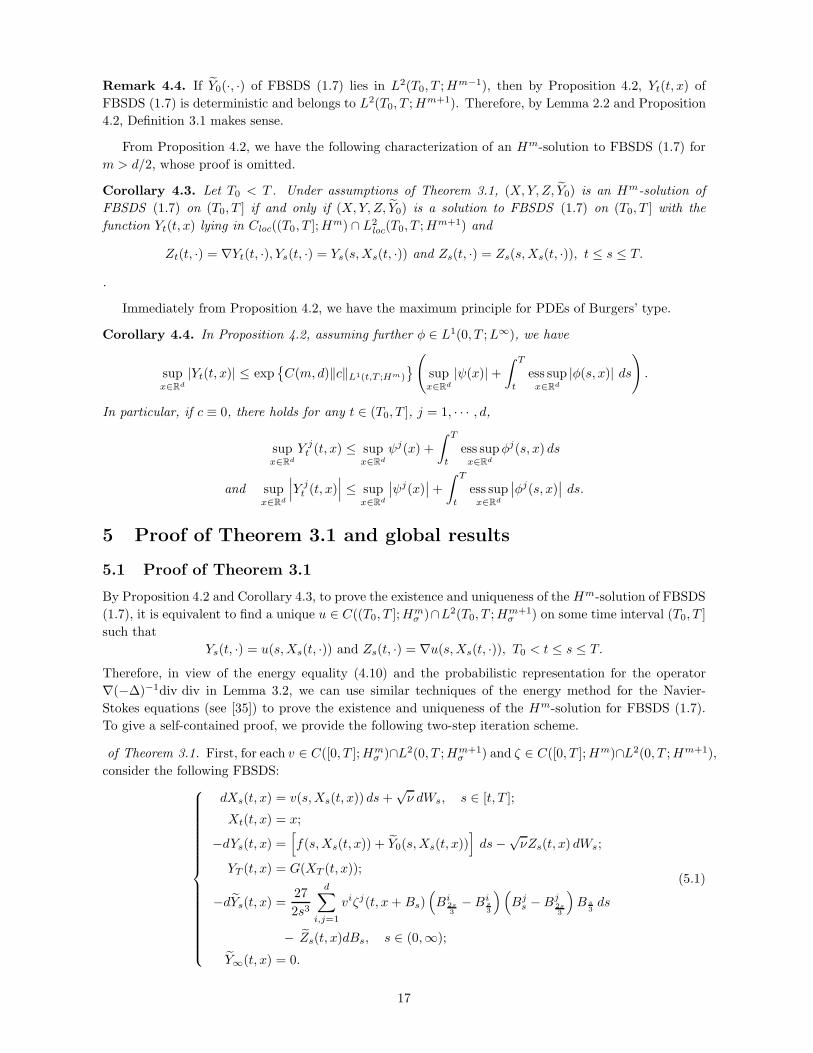
Remark 4.4. If Y0(·, ·) of FBSDS (1.7) lies in L2(T0, T ;Hm−1), then by Proposition 4.2, Yt(t, x) of

FBSDS (1.7) is deterministic and belongs to L2(T0, T ;Hm+1). Therefore, by Lemma 2.2 and Proposition

4.2, Definition 3.1 makes sense.

From Proposition 4.2, we have the following characterization of an Hm-solution to FBSDS (1.7) for

m > d/2, whose proof is omitted.

Corollary 4.3. Let T0 < T . Under assumptions of Theorem 3.1, (X,Y, Z, Y0) is an Hm-solution of

FBSDS (1.7) on (T0, T ] if and only if (X,Y, Z, Y0) is a solution to FBSDS (1.7) on (T0, T ] with the

function Yt(t, x) lying in Cloc((T0, T ];Hm) ∩ L2

loc(T0, T ;H

m+1) and

Zt(t, ·) = ∇Yt(t, ·), Ys(t, ·) = Ys(s,Xs(t, ·)) and Zs(t, ·) = Zs(s,Xs(t, ·)), t ≤ s ≤ T.

.

Immediately from Proposition 4.2, we have the maximum principle for PDEs of Burgers’ type.

Corollary 4.4. In Proposition 4.2, assuming further φ ∈ L1(0, T ;L∞), we have

supx∈Rd

|Yt(t, x)| ≤ expC(m, d)‖c‖L1(t,T ;Hm)

(supx∈Rd

|ψ(x)| +∫ T

t

ess supx∈Rd

|φ(s, x)| ds).

In particular, if c ≡ 0, there holds for any t ∈ (T0, T ], j = 1, · · · , d,

supx∈Rd

Y jt (t, x) ≤ sup

x∈Rd

ψj(x) +

∫ T

t

ess supx∈Rd

φj(s, x) ds

and supx∈Rd

∣∣∣Y jt (t, x)

∣∣∣ ≤ supx∈Rd

∣∣ψj(x)∣∣+∫ T

t

ess supx∈Rd

∣∣φj(s, x)∣∣ ds.

5 Proof of Theorem 3.1 and global results

5.1 Proof of Theorem 3.1

By Proposition 4.2 and Corollary 4.3, to prove the existence and uniqueness of the Hm-solution of FBSDS

(1.7), it is equivalent to find a unique u ∈ C((T0, T ];Hmσ )∩L2(T0, T ;H

m+1σ ) on some time interval (T0, T ]

such that

Ys(t, ·) = u(s,Xs(t, ·)) and Zs(t, ·) = ∇u(s,Xs(t, ·)), T0 < t ≤ s ≤ T.

Therefore, in view of the energy equality (4.10) and the probabilistic representation for the operator

∇(−∆)−1div div in Lemma 3.2, we can use similar techniques of the energy method for the Navier-

Stokes equations (see [35]) to prove the existence and uniqueness of the Hm-solution for FBSDS (1.7).

To give a self-contained proof, we provide the following two-step iteration scheme.

of Theorem 3.1. First, for each v ∈ C([0, T ];Hmσ )∩L2(0, T ;Hm+1

σ ) and ζ ∈ C([0, T ];Hm)∩L2(0, T ;Hm+1),

consider the following FBSDS:

dXs(t, x) = v(s,Xs(t, x)) ds +√ν dWs, s ∈ [t, T ];

Xt(t, x) = x;

−dYs(t, x) =[f(s,Xs(t, x)) + Y0(s,Xs(t, x))

]ds−

√νZs(t, x) dWs;

YT (t, x) = G(XT (t, x));

−dYs(t, x) =27

2s3

d∑

i,j=1

viζj(t, x+ Bs)(Bi

2s3−Bi

s3

)(Bj

s −Bj2s3

)B s

3ds

− Zs(t, x)dBs, s ∈ (0,∞);

Y∞(t, x) = 0.

(5.1)

17

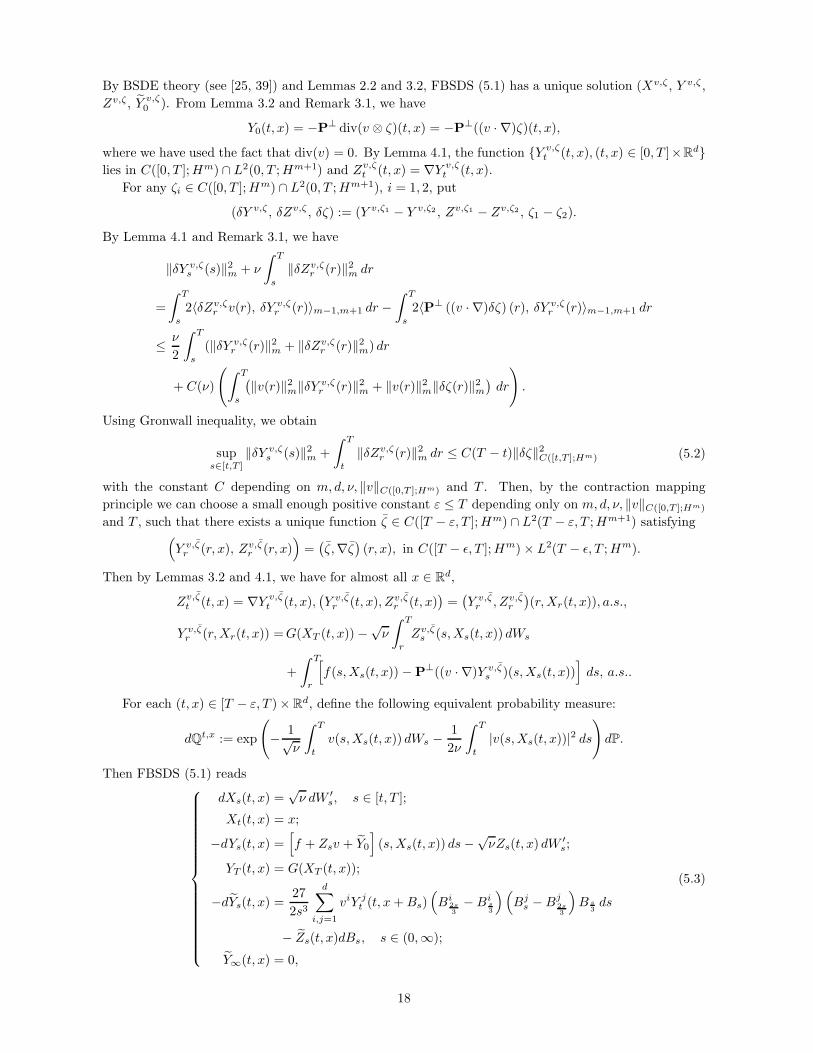
By BSDE theory (see [25, 39]) and Lemmas 2.2 and 3.2, FBSDS (5.1) has a unique solution (Xv,ζ , Y v,ζ ,

Zv,ζ, Y v,ζ0 ). From Lemma 3.2 and Remark 3.1, we have

Y0(t, x) = −P⊥ div(v ⊗ ζ)(t, x) = −P⊥((v · ∇)ζ)(t, x),

where we have used the fact that div(v) = 0. By Lemma 4.1, the function Y v,ζt (t, x), (t, x) ∈ [0, T ]×Rd

lies in C([0, T ];Hm) ∩ L2(0, T ;Hm+1) and Zv,ζt (t, x) = ∇Y v,ζ

t (t, x).

For any ζi ∈ C([0, T ];Hm) ∩ L2(0, T ;Hm+1), i = 1, 2, put

(δY v,ζ , δZv,ζ , δζ) := (Y v,ζ1 − Y v,ζ2 , Zv,ζ1 − Zv,ζ2 , ζ1 − ζ2).

By Lemma 4.1 and Remark 3.1, we have

‖δY v,ζs (s)‖2m + ν

∫ T

s

‖δZv,ζr (r)‖2m dr

=

∫ T

s

2〈δZv,ζr v(r), δY v,ζ

r (r)〉m−1,m+1 dr −∫ T

s

2〈P⊥ ((v · ∇)δζ) (r), δY v,ζr (r)〉m−1,m+1 dr

≤ ν

2

∫ T

s

(‖δY v,ζr (r)‖2m + ‖δZv,ζ

r (r)‖2m) dr

+ C(ν)

(∫ T

s

(‖v(r)‖2m‖δY v,ζ

r (r)‖2m + ‖v(r)‖2m‖δζ(r)‖2m)dr

).

Using Gronwall inequality, we obtain

sups∈[t,T ]

‖δY v,ζs (s)‖2m +

∫ T

t

‖δZv,ζr (r)‖2m dr ≤ C(T − t)‖δζ‖2C([t,T ];Hm) (5.2)

with the constant C depending on m, d, ν, ‖v‖C([0,T ];Hm) and T . Then, by the contraction mapping

principle we can choose a small enough positive constant ε ≤ T depending only on m, d, ν, ‖v‖C([0,T ];Hm)

and T , such that there exists a unique function ζ ∈ C([T − ε, T ];Hm) ∩ L2(T − ε, T ;Hm+1) satisfying(Y v,ζr (r, x), Zv,ζ

r (r, x))=(ζ,∇ζ

)(r, x), in C([T − ǫ, T ];Hm)× L2(T − ǫ, T ;Hm).

Then by Lemmas 3.2 and 4.1, we have for almost all x ∈ Rd,

Zv,ζt (t, x) = ∇Y v,ζ

t (t, x),(Y v,ζr (t, x), Zv,ζ

r (t, x))=(Y v,ζr , Zv,ζ

r

)(r,Xr(t, x)), a.s.,

Y v,ζr (r,Xr(t, x)) =G(XT (t, x))−

√ν

∫ T

r

Zv,ζs (s,Xs(t, x)) dWs

+

∫ T

r

[f(s,Xs(t, x)) −P⊥((v · ∇)Y v,ζ

s )(s,Xs(t, x))]ds, a.s..

For each (t, x) ∈ [T − ε, T )× Rd, define the following equivalent probability measure:

dQt,x := exp

(− 1√

ν

∫ T

t

v(s,Xs(t, x)) dWs −1

2ν

∫ T

t

|v(s,Xs(t, x))|2 ds)dP.

Then FBSDS (5.1) reads

dXs(t, x) =√ν dW ′

s, s ∈ [t, T ];

Xt(t, x) = x;

−dYs(t, x) =[f + Zsv + Y0

](s,Xs(t, x)) ds−

√νZs(t, x) dW

′s;

YT (t, x) = G(XT (t, x));

−dYs(t, x) =27

2s3

d∑

i,j=1

viY jt (t, x+Bs)

(Bi

2s3−Bi

s3

)(Bj

s −Bj2s3

)B s

3ds

− Zs(t, x)dBs, s ∈ (0,∞);

Y∞(t, x) = 0,

(5.3)

18

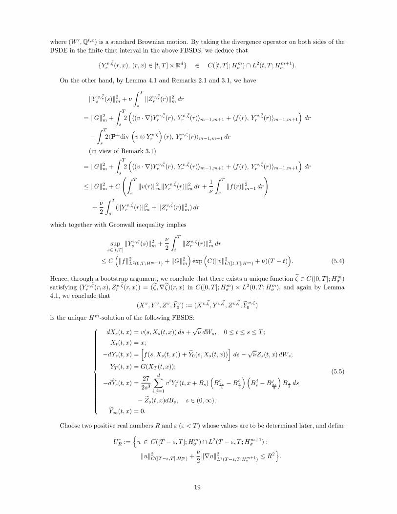
where (W ′,Qt,x) is a standard Brownian motion. By taking the divergence operator on both sides of the

BSDE in the finite time interval in the above FBSDS, we deduce that

Y v,ζr (r, x), (r, x) ∈ [t, T ]× Rd ∈ C([t, T ];Hm

σ ) ∩ L2(t, T ;Hm+1σ ).

On the other hand, by Lemma 4.1 and Remarks 2.1 and 3.1, we have

‖Y v,ζs (s)‖2m + ν

∫ T

s

‖Zv,ζr (r)‖2m dr

= ‖G‖2m +

∫ T

s

2(〈(v · ∇)Y v,ζ

r (r), Y v,ζr (r)〉m−1,m+1 + 〈f(r), Y v,ζ

r (r)〉m−1,m+1

)dr

−∫ T

s

2〈P⊥div(v ⊗ Y v,ζ

r

)(r), Y v,ζ

r (r)〉m−1,m+1 dr

(in view of Remark 3.1)

= ‖G‖2m +

∫ T

s

2(〈(v · ∇)Y v,ζ

r (r), Y v,ζr (r)〉m−1,m+1 + 〈f(r), Y v,ζ

r (r)〉m−1,m+1

)dr

≤ ‖G‖2m + C

(∫ T

s

‖v(r)‖2m‖Y v,ζr (r)‖2m dr +

1

ν

∫ T

s

‖f(r)‖2m−1 dr

)

+ν

2

∫ T

s

(‖Y v,ζr (r)‖2m + ‖Zv,ζ

r (r)‖2m) dr

which together with Gronwall inequality implies

sups∈[t,T ]

‖Y v,ζs (s)‖2m +

ν

2

∫ T

t

‖Zv,ζr (r)‖2m dr

≤ C(‖f‖2L2(0,T ;Hm−1) + ‖G‖2m

)exp

(C(‖v‖2C([t,T ];Hm) + ν)(T − t)

). (5.4)

Hence, through a bootstrap argument, we conclude that there exists a unique function ζ ∈ C([0, T ];Hmσ )

satisfying (Y v,ζr (r, x), Zv,ζ

r (r, x)) = (ζ ,∇ζ)(r, x) in C([0, T ];Hmσ ) × L2(0, T ;Hm

σ ), and again by Lemma

4.1, we conclude that

(Xv, Y v, Zv, Y v0 ) := (Xv,ζ, Y v,ζ , Zv,ζ , Y v,ζ

0 )

is the unique Hm-solution of the following FBSDS:

dXs(t, x) = v(s,Xs(t, x)) ds +√ν dWs, 0 ≤ t ≤ s ≤ T ;

Xt(t, x) = x;

−dYs(t, x) =[f(s,Xs(t, x)) + Y0(s,Xs(t, x))

]ds−

√νZs(t, x) dWs;

YT (t, x) = G(XT (t, x));

−dYs(t, x) =27

2s3

d∑

i,j=1

viY jt (t, x+Bs)

(Bi

2s3−Bi

s3

)(Bj

s −Bj2s3

)B s

3ds

− Zs(t, x)dBs, s ∈ (0,∞);

Y∞(t, x) = 0.

(5.5)

Choose two positive real numbers R and ε (ε < T ) whose values are to be determined later, and define

UεR :=

u ∈ C([T − ε, T ];Hm

σ ) ∩ L2(T − ε, T ;Hm+1σ ) :

‖u‖2C([T−ε,T ];Hmσ ) +

ν

2‖∇u‖2

L2(T−ε,T ;Hm+1σ )

≤ R2.

19

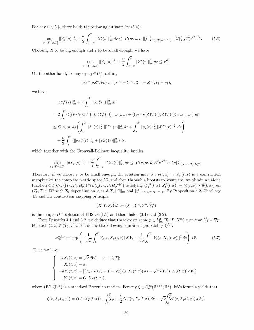
For any v ∈ UεR, there holds the following estimate by (5.4):

sups∈[T−ε,T ]

‖Y vs (s)‖2m +

ν

2

∫ T

T−ε

‖Zvs (s)‖2m dr ≤ C(m, d, ν, ‖f‖2L2(0,T ;Hm−1), ‖G‖2m, T )eCR2ε. (5.6)

Choosing R to be big enough and ε to be small enough, we have

sups∈[T−ε,T ]

‖Y vs (s)‖2m +

ν

2

∫ T

T−ε

‖Zvr (r)‖2m dr ≤ R2.

On the other hand, for any v1, v2 ∈ UεR, setting

(δY v, δZv, δv) := (Y v1 − Y v2 , Zv1 − Zv2 , v1 − v2),

we have

‖δY vs (s)‖2m + ν

∫ T

s

‖δZvr (r)‖2m dr

= 2

∫ T

s

(〈(δv · ∇)Y v1r (r), δY v

r (r)〉m−1,m+1 + 〈(v2 · ∇)δY vr (r), δY

vr (r)〉m−1,m+1) dr

≤ C(ν,m, d)

(∫ T

s

‖δv(r)‖2m‖Y v1r (r)‖2m dr +

∫ T

s

‖v2(r)‖2m‖δY vr (r)‖2m dr

)

+ν

2

∫ T

s

(‖δY vr (r)‖2m + ‖δZv

r (r)‖2m) dr,

which together with the Gronwall-Bellman inequality, implies

sups∈[T−ε,T ]

‖δY vs (s)‖2m +

ν

2

∫ T

T−ε

‖δZvr (r)‖2m dr ≤ C(ν,m, d)R2eR

2T ε‖δv‖2C([T−ε,T ];Hmσ ).

Therefore, if we choose ε to be small enough, the solution map Ψ : v(t, x) 7→ Y vt (t, x) is a contraction

mapping on the complete metric space UεR and then through a bootstrap argument, we obtain a unique

function u ∈ Cloc((T0, T ];Hmσ ) ∩ L2

loc(T0, T ;Hm+1σ ) satisfying (Y u

t (t, x), Z ut (t, x)) = (u(t, x),∇u(t, x)) on

(T0, T ]× Rd with T0 depending on ν,m, d, T, ‖G‖m and ‖f‖L2(0,T ;Hm−1). By Proposition 4.2, Corollary

4.3 and the contraction mapping principle,

(X,Y, Z, Y0) := (X u, Y u, Z u, Y u0 )

is the unique Hm-solution of FBSDS (1.7) and there holds (3.1) and (3.2).

From Remarks 3.1 and 3.2, we deduce that there exists some p ∈ L2loc(T0, T ;H

m) such that Y0 = ∇p.For each (t, x) ∈ (T0, T ]× Rd, define the following equivalent probability Qt,x:

dQt,x := exp

(− 1√

ν

∫ T

t

Ys(s,Xs(t, x)) dWs −1

2ν

∫ T

t

|Ys(s,Xs(t, x))|2 ds)dP. (5.7)

Then we have

dXs(t, x) =√ν dW ′

s, s ∈ [t, T ];

Xt(t, x) = x;

−dYs(t, x) = [(Ys · ∇)Ys + f +∇p] (s,Xs(t, x)) ds −√ν∇Ys(s,Xs(t, x)) dW

′s;

YT (t, x) = G(XT (t, x)),

where (W ′,Qt,x) is a standard Brownian motion. For any ζ ∈ C∞c (R1+d;Rd), Ito’s formula yields that

ζ(s,Xs(t, x)) = ζ(T,XT (t, x)) −∫ T

s

(∂r +ν

2∆)ζ(r,Xr(t, x))dr −

√ν

∫ T

s

∇ζ(r,Xr(t, x)) dW′r ,

20

and thus,

EQt,x [〈Yt, ζ〉(t, x)] + νE

[ ∫ T

t

〈∇ζ, ∇Ys〉(s,Xs(t, x)) ds

]

=EQt,x

[∫ T

t

(〈−∂sζ −ν

2∆ζ, Ys〉+ 〈ζ, (Ys · ∇)Ys +∇p+ f〉)(s,Xs(t, x)) ds

+ 〈ζ(T,XT (t, x)), G(xT (t, x))〉].

Integrating both sides in x, we obtain

〈ζ(t), Yt(t)〉0 =

∫ T

t

[− 〈∂sζ(s), Ys(s)〉0 + 〈ζ(s), ν

2∆Ys(s) + (Ys · ∇)Ys(s) +∇p(s) + f(s)〉0

]ds

+ 〈ζ(T ), G〉0

Hence, (Yt(t, x), p(t, x)) is a strong solution to Navier-Stokes equation (1.1) (see [51, 52]). Due to the

reversibility of the above procedure, the uniqueness of the Hm-solution of FBSDS (1.7) implies that of

the strong solution for Navier-Stokes equation (1.1) as well. The proof is complete.

Remark 5.1. In the above proof, Proposition 4.2 plays a crucial role in the characterization of the

solution of FBSDS (1.7) (see Corollary 4.3). This characterization together with the contraction principle

serves to guarantee the existence and uniqueness of the Hm-solution of FBSDS (1.7).

5.2 Global results

By Lemma 3.2, Proposition 4.2 and Corollary 4.3, basing on the energy equality (4.10) we can also obtain

the global results in a similar way to the energy method for the Navier-Stokes (see [35, Page 86–134]).

First, for the two dimensional case, we can obtain the following global result in a similar way to [35,

Section 3.3]. We omit the proof herein.

Proposition 5.1. Let d = 2, m ≥ 3 and G ∈ Hmσ . Then FBSDS (1.7) with f = 0 admits a unique

Hm-solution (X,Y, Z, Y0) on [0, T ].

The other global result is for the case of small Reynolds numbers. Let us work on the d-dimensional

torus Td = Rd/(L × Zd) where L > 0 is a fixed length scale. Denote by (Hn,qσ (Td;Rd), ‖ · ‖n,q;Td) the

Rd-valued Sobolev space on Td, each element of which is divergence free. For q = 2, write (Hnσ (T

d;Rd), ‖·‖n;Td) for simplicity. Let f = 0 and G ∈ Hm

σ (Td;Rd) of zero mean for m > d/2. In a similar way to

Theorem 3.1, FBSDS (1.7) defined on torus admits a unique Hm-solution (X,Y, Z, Y0) on some interval

(T0, T ]. Moreover, we have

‖Yt(t)‖2m;Td + ν

∫ T

t

‖Zs(s)‖2m;Td ds

= ‖G‖2m;Td + 2

∫ T

t

〈Zs(s)Ys(s), Ys(s)〉m−1,m+1;Td ds

≤ ‖G‖2m;Td + C

∫ T

t

‖Ys(s)‖m;Td‖Zs(s)‖m−1;Td‖Ys(s)‖m+1;Td ds

≤ ‖G‖2m;Td + C

∫ T

t

‖Ys(s)‖m;Td‖Zs(s)‖m−1;Td

(‖Ys(s)‖m;Td + ‖Zs(s)‖m;Td

)ds

≤ ‖G‖2m;Td + CL

∫ T

t

‖Ys(s)‖m;Td‖Zs(s)‖2m;Td ds,

where Zs(s, ·) = ∇Ys(s, ·) and we have used the Poincare inequality

‖Ys(s, ·)‖m;Td ≤ CL‖∇Ys(s, ·)‖m;Td , s ∈ [t, T ],

21

with Ys(s, ·) being mean zero and the constant C being independent of L. Thus,

‖Yt(t)‖2m;Td +

∫ T

t

(ν − CL‖Ys(s)‖m;Td)‖Zs(s)‖2m;Td ds ≤ ‖G‖2m;Td .

If we take the Reynolds number R := Lν−1‖G‖m;Td < C−1, then for this local solution (X,Y, Z, Y0) we

always have

‖Yt(t, ·)‖m;Td ≤ ‖G‖m;Td , t ∈ (T0, T ].

Using bootstrap arguments, the local solution can be extended to be a global one. In summary, we have

Proposition 5.2. Assume that f = 0 and G ∈ Hmσ (Td;Rd) (m > d/2) is mean zero. Then FBSDS (1.7)

admits a unique Hm-solution (X,Y, Z, Y0) on some time interval (T0, T ] with Yt(t, x) being spacial mean

zero. Moreover, there exists a positive constant R0 (= C−1 as above) such that if the Reynolds number

R < R0, the local Hm-solution can be extended to be a time global one and for this global Hm-solution

we have

‖Yt(t)‖m;Td ≤ ‖G‖m;Td , for any t ∈ [0, T ].

Remark 5.2. FBSDS (1.7) is a complicated version of FBSDE (1.3), including an additional nonlinear

and nonlocal term in the drift of the BSDE to keep the backward state living in the divergence-free

subspace. While the additional term causes difficulty in formulating probabilistic representations, it

helps us to obtain the global solutions in Propositions 5.1 and 5.2.

6 Approximation of the Navier-Stokes equation

In view of FBSDS (1.7) and Theorem 3.1, the Navier-Stokes equation is approximated in this section by

truncating the time interval of the BSDE associated with Y .

Lemma 6.1. For k ∈ N, γ, α ∈ (0, 1), γ ≤ α, there is a constant C such that

‖φ‖Ck,γ ≤ C‖φ‖Ck,α , ∀φ ∈ Ck,α,

‖φ‖Ck,α ≤ C (‖φ‖Ck,γ + ‖∇φ‖Ck) , ∀φ ∈ Ck+1.

It is an immediate consequence of the interpolation inequalities of Gilbarg and Trudinger [27, Lemma

6.32].

To approximate the Navier-Stokes equations, we truncate the time interval of the infinite-time-interval

BSDE of FBSDS (1.7).

Lemma 6.2. For any φ, ψ ∈ Ck,α, k ∈ Z+, α ∈ (0, 1), the following BSDE

−dYs(x) =27

2s3

d∑

i,j=1

φiψj(x+Bs)(Bj

s − Bj2s3

)(Bi

2s3−Bi

s3

)B s

3ds

− Zs(t, x)dBs, s ∈ (0,∞)

Y∞(x) = 0

(6.1)

is well-posed on the time interval (0,∞) and Y0(x) := limε↓0 EYε(x) exists for each x ∈ Rd. Moreover,

Y0 = ∇(−∆)−1div div(φ⊗ ψ) ∈ Ck−1,α2 ,

and

‖Y0‖Ck−1, α2≤ C‖φ‖Ck,α‖ψ‖Ck,α , (6.2)

with the positive constant C independent of φ and ψ.

22

Sketched only. For any ε ∈ (0, 1) and N ∈ (1,∞), in a similar way to the proof of Lemma 3.2,

∣∣∣∣E∫ N

ε

27

2s3φiψj(x+Bs)

(Bj

s −Bj2s3

)(Bi

2s3−Bi

s3

)B s

3ds

∣∣∣∣

=

∣∣∣∣E(∫ 1

ε

+

∫ N

1

)27

2s3φiψj(x +Bs)

(Bj

s −Bj2s3

)(Bi

2s3−Bi

s3

)B s

3ds

∣∣∣∣

=

∣∣∣∣E∫ 1

ε

9

2s2[∇(φiψj)(x+Bs)−∇(φiψj)(x)

] (Bj

s −Bj2s3

)(Bi

2s3−Bi

s3

)ds

+ E

∫ N

1

27

2s3φiψj(x+Bs)

(Bj

s −Bj2s3

)(Bi

2s3−Bi

s3

)B s

3ds

∣∣∣∣

≤C‖φ⊗ ψ‖C1,α

∫ 1

ε

1

s1−α2ds+ C‖φ⊗ ψ‖L∞

∫ N

1

1

s32

ds

≤C‖φ⊗ ψ‖C1,α

(2− ε

α2 − 1√

N

), i, j = 1, · · · , d. (6.3)

Letting N → ∞ and ε → 0, we conclude that BSDE (6.1) is well-posed on the time interval (0,∞) and

Y0(x) := limε↓0 EYε(x) exists for each x ∈ Rd.

On the other hand, for each x, y ∈ Rd, i, j = 1, · · · , d,∣∣∣∣E∫ N

1

27

2s3(φiψj(x+Bs)− φiψj(y +Bs)

) (Bj

s −Bj2s3

)(Bi

2s3−Bi

s3

)B s

3ds

∣∣∣∣

≤ C|x − y|α2 ‖φ⊗ ψ‖12

C1,α‖φ⊗ ψ‖12

L∞E

∫ N

1

1

s3

∣∣∣(Bj

s −Bj2s3

)(Bi

2s3−Bi

s3

)B s

3

∣∣∣ ds

≤ C|x − y|α2 ‖φ⊗ ψ‖C1,α

(1− 1√

N

)(6.4)

and∣∣∣∣E∫ 1

ε

9

2s2[∇(φiψj)(x+Bs)−∇(φiψj)(y +Bs)

] (Bj

s −Bj2s3

)(Bi

2s3−Bi

s3

)ds

∣∣∣∣

=

∣∣∣∣E∫ 1

ε

9

2s2∇[φi(x+Bs)

(ψj(x+Bs)− ψj(y + Bs)

)+(φi(x+Bs)− φi(y +Bs)

)ψj(y +Bs)

]

(Bj

s −Bj2s3

)(Bi

2s3−Bi

s3

)ds

∣∣∣∣

=

∣∣∣∣E∫ 1

ε

9

2s2∇[ (φi(x +Bs)− φi(x)

) (ψj(x+Bs)− ψj(y +Bs)

)

+ φi(x)(ψj(x+Bs)− ψj(x) − ψj(y +Bs) + ψj(y)

)

+(φi(x+Bs)− φi(y +Bs)

) (ψj(y +Bs)− ψj(y)

)

+ ψj(y)(φi(x+Bs)− φi(x)− φi(y +Bs) + φi(y)

) ] (Bj

s −Bj2s3

)(Bi

2s3−Bi

s3

)ds

∣∣∣∣

≤ C|x− y|α2 ‖φ‖C1,α‖ψ‖C1,αE

∫ 1

ε

1

s2

∣∣∣|Bs|α2

(Bj

s −Bj2s3

)(Bi

2s3−Bi

s3

)∣∣∣ ds

≤ C|x− y|α2 ‖φ‖C1,α‖ψ‖C1,α

(1− ε

α4

), (6.5)

where for h = φi, ∇φi, ψj or ∇ψj , we note that

|h(x+Bs)− h(x) − h(y +Bs) + h(y)|

≤ |h(x+Bs)− h(x) − h(y +Bs) + h(y)|12

(|h(x+Bs)− h(x)|

12 + |h(y +Bs) + h(y)|

12

)

≤4 ‖h‖C1,α |Bs|α2 |x− y|α2 .

23

Hence, combining (6.3), (6.4) and (6.5), we obtain

‖Y0‖C0, α2≤ C‖φ‖C1,α‖ψ‖C1,α .

Taking k − 1-th derivatives in the above arguments, we prove (6.2).

Remark 6.1. In view of (6.4) and (6.5) of the above proof, we can deduce easily that for any ε ∈ (0, 1)

and N ∈ (1,∞),

∥∥∥E[Yε − YN

]∥∥∥Ck−1, α

2

≤ C‖φ‖Ck,α‖ψ‖Ck,α

(2− ε

α4 − 1√

N

)

with the constant C independent of φ, ψ, ε and N . Moreover, in a similar way to the above proof, we

obtain

‖E[Yε − YN − Y0

]‖Ck−1, α

2≤ C

(ε

α4 +

1√N

)‖φ‖Ck,α‖ψ‖Ck,α ,

with the constant C independent of φ, ψ, ε and N .

Define the heat kernel

Hν(t, x) :=1

(2πνt)d2

exp(− |x|2

2νt

),

and the convolution

Hν(t) ∗ g(x) =∫

Rd

Hν(t, x− y)g(y) dy, ∀ g ∈ C(Rd).

Lemma 6.3. There is a constant C such that for any φ ∈ Ck,γ with k ∈ N and γ ∈ (0, 1),

‖Hν(t) ∗ φ‖Ck+1,γ ≤C

(1 +

1√νt

)‖φ‖Ck,γ ; (6.6)

d∑

i,j=1

‖∂xi∂xjHν(t) ∗ φ‖Ck ≤ C

(νt)1−γ4

‖φ‖Ck,

γ2; (6.7)

‖Hν(t) ∗ φ‖Ck+1,γ ≤C

(1 +

1√νt

+1

(νt)1−γ4

)‖φ‖

Ck,γ2. (6.8)

Sketched only. The estimate (6.6) follows from

|Hν(t) ∗ φ(x)| =∣∣∣∣∫

Rd

Hν(t, x− y)φ(y) dy

∣∣∣∣ ≤ ‖φ‖C(Rd), ∀x ∈ Rd

and for any x, z ∈ Rd,

|∇Hν(t) ∗ φ(x) −∇Hν(t) ∗ φ(z)| =∣∣∣∣∣

∫

Rd

y

(2π)d2 (νt)

d2+1

exp(− |y|2

2νt

)(φ(x − y)− φ(z − y)) dy

∣∣∣∣∣

≤ |x− z|γ‖φ‖C0,γ

∫

Rd

|y|(2π)

d2 (νt)

d2+1

exp(− |y|2

2νt

)dy

≤ C√νt

|x− z|γ‖φ‖C0,γ .

For any x ∈ Rd and i, j = 1, · · · , d,

|∂xi∂xjHν(t) ∗ φ(x)| =∣∣∣∣∣

∫

Rd

1

(2πνt)d2

( |y|2(tν)2

− 1

νt

)exp(− |y|2

2νt

)(φ(x − y)− φ(x)) dy

∣∣∣∣∣

24

≤‖φ‖C0,

γ2

∫

Rd

|y| γ2(2πνt)

d2

( |y|2(tν)2

+1

νt

)exp(− |y|2

2νt

)dy

≤ C

(νt)1−γ4

‖φ‖C0,

γ2,

which implies estimate (6.7).

Finally,

‖Hν(t) ∗ φ‖Ck+1,γ ≤C(‖Hν(t) ∗ φ‖

Ck+1,γ2+ ‖∇Hν(t) ∗ φ‖Ck+1

)(by Lemma 6.2)

≤C

‖Hν(t) ∗ φ‖

Ck+1,γ2+

d∑

i,j=1

‖∂xi∂xjHν(t) ∗ φ‖Ck

≤C

(1 +

1√νt

+1

(νt)1−γ4

)‖φ‖

Ck,γ2

(by estimates (6.6) and (6.7)).

The proof is completed.

For each N ∈ (1,∞), define

PN (φ⊗ ψ) = E[Y 1

N− YN

], φ, ψ ∈ Hm, m >

d

2+ 1,

where Y· satisfies BSDE (6.1). In view of Remark 3.3, we have

‖PN (φ⊗ ψ)‖k ≤ C

(1√N

+√N

)‖φ⊗ ψ‖k, 0 ≤ k ≤ m. (6.9)

In a similar way to Theorem 3.1, we have

Theorem 6.4. Let ν > 0, G ∈ Hm, and f ∈ L2(0, T ;Hm−1) with m > d/2. Then there is T0 < T which

depends on ‖f‖L2(0,T ;Hm−1), ν, m, d, T , N and ‖G‖m, such that FBSDS

dXs(t, x) = Ys(t, x) ds+√ν dWs, s ∈ [t, T ];

Xt(t, x) = x;

−dYs(t, x) =[f(s,Xs(t, x)) + Y0(s,Xs(t, x))

]ds−

√νZs(t, x) dWs;

YT (t, x) = G(XT (t, x));

−dYs(t, x) =d∑

i,j=1

27

2s3Y it Y

jt (t, x+Bs)

(Bi

2s3−Bi

s3

)(Bj

s −Bj2s3

)B s

3I[ 1

N,N](s) ds

− Zs(t, x)dBs, s ∈ (0,∞);

Y∞(t, x) = 0.

(6.10)

has a unique Hm-solution (X,Y, Z, Y0) on (T0, T ] with

Yt(t, x), (t, x) ∈ (T0, T ]× Rd ∈ Cloc((T0, T ];Hm) ∩ L2

loc(T0, T ;Hm+1).

Moreover, we have

Zt(t, ·) = ∇Yt(t, ·), Ys(t, ·) = Ys(s,Xs(t, ·)) and Zs(t, ·) = Zs(s,Xs(t, ·)), (6.11)

for T0 < t ≤ s ≤ T , (Y, Z, Y0) satisfies

Yr(r,Xr(t, x)) =G(XT (t, x)) +

∫ T

r

[f(s,Xs(t, x)) + Y0(s,Xs(t, x))

]ds

25

−√ν

∫ T

r

Zs(s,Xs(t, x)) dWs, T0 < t ≤ r ≤ T, a.e.x ∈ Rd, a.s., (6.12)

and uN(r, x) := Yr(r, x) is the unique strong solution of the following PDE:

∂tu

N + ν2∆u

N + (uN · ∇)uN +PN (uN ⊗ uN) + f = 0, T0 < t ≤ T ;

uN(T ) = G.(6.13)

The proof is similar to that of Theorem 3.1, and is omitted here.

Letting r = t, using Girsanov transformation in a similar way to (5.1) of the proof for Theorem 3.1

and then taking expectations on both sides of (6.12), we have

uN (t, x) = Hν(T − t) ∗G(x) +∫ T

t

Hν(s− t) ∗(f + (uN · ∇)uN +PN (uN ⊗ uN )

)(s, x) ds. (6.14)

Assume

G ∈ Ck,α, f ∈ C([0, T ];Ck−1,α), k ∈ Z+, α ∈ (0, 1). (6.15)

By Lemmas 6.2 and 6.3 and in view of Remark 6.1, we get

‖uN(t)‖Ck,α ≤C‖G‖Ck,α + C

∫ T

t

[(1 +

1√s− t

)(‖f(s) + (uN · ∇)uN (s)‖Ck−1,α

+(1 +

1√s− t

+1

(s− t)1−α4

)‖PN (uN ⊗ uN)(s)‖

Ck−1, α2

]ds

≤C‖G‖Ck,α + C

∫ T

t

[(1 +

1√s− t

)(‖f(s)‖Ck−1,α + ‖uN(s)‖2Ck,α

)

+(1 +

1√s− t

+1

(s− t)1−α4

)‖uN(s)‖2Ck,α

]ds

≤C‖G‖Ck,α + C‖f‖C([0,T ];Ck−1,α) + C

∫ T

t

(1 +

1

(s− t)1−α4

)‖uN(s)‖2Ck,α ds, (6.16)

which by Gronwall inequality implies that

sups∈[t,T ]

‖uN(s)‖Ck,α ≤C(‖G‖Ck,α + ‖f‖C([0,T ];Ck−1,α)

)

1− C2(‖G‖Ck,α + ‖f‖C([0,T ];Ck−1,α))[(T − t) + (T − t)

α4

] , (6.17)

where T − t is small enough and the constant C is independent of t and N . In view of (6.7) of Lemma

6.3, we further have uN (t) ∈ Ck+1 when t is away from T .

From estimate (6.17) and Theorem 6.4, similar to Theorem 3.1, we have the following corollary.

Corollary 6.5. Let ν > 0. Under assumption (6.15), there is T1 < T which depends on ‖f‖C([0,T ];Ck−1,α),

ν, T and ‖G‖Ck,α, such that FBSDS (6.10) has a unique solution (X,Y, Z, Y0) on (T1, T ] with

Yr(r, x), (r, x) ∈ (T1, T ]× Rd ∈ Cloc((T1, T ];Ck,α) ∩ Cloc((T1, T );C

k+1) and Zr(r, x) = ∇Yr(r, x).

Moreover, we have (6.11), (Y, Z, Y0) satisfies BSDE (6.12), and uN(r, x) := Yr(r, x) is the unique solution

of the PDE (6.13).

Since Cl,α∩Hm is dense in Cl,α for any m > d2 and l ∈ N, by Theorem 6.4 we can prove the existence

of the solution (X,Y, Z, Y0) through standard density arguments. In view of representation (6.14), we can

prove the uniqueness of the solution through a priori estimates in a similar way to (6.16). From estimate

(6.17), the unique solution can be extended to the maximal time interval (T1, T ]. The proof of Corollary

6.5 is omitted. It is worth noting that T1 is independent of N in Corollary 6.5, while in Theorem 6.4 T0depends on N .

Now we shall use the solution uN of PDE (6.13) to approximate the velocity field u of Navier-Stokes

equation (1.1).

26

Theorem 6.6. Let ν > 0, G ∈ Hmσ , and f ∈ C([0, T ];Hm−1

σ ) with m > d2 + 1. Let

u ∈ Cloc((T0, T ];Hmσ ) ∩ L2

loc(T0, T ;Hm+1σ )

be the strong solution of Navier-Stokes equation (1.1) in Theorem 3.1. Since

Hm → Ck−1,α, for some k ∈ Z+ and α ∈ (0, 1),

we are allowed to assume that uN ∈ Cloc((T1, T ];Ck,α)∩Cloc((T1, T );C

k+1) be the solution of PDE (6.13)

in Corollary 6.5. Then, for any t ∈ (T0 ∧ T1, T ], there exists a constant C independent of N such that

∥∥u− uN∥∥C(t,T ;Ck,α)

≤ C

Nα4. (6.18)

Proof. In a similar way to (6.14), we get for any τ ∈ [t, T ]

u(τ, x) = Hν(T − τ) ∗G(x) +∫ T

τ

Hν(s− τ) ∗(f + (u · ∇)u −P⊥ div (u⊗ u)

)(s, x) ds.

Putting δu = uN − u, we have for τ ∈ [t, T ]

δu(τ, x)

=

∫ T

τ

Hν(s− τ) ∗((uN · ∇)uN − (u · ∇)u+PN (uN ⊗ uN) +P⊥ div (u⊗ u)

)(s, x) ds

=

∫ T

τ

Hν(s− τ) ∗((δu · ∇)uN+ (u · ∇)δu + (PN+P⊥ div )(u ⊗ u) +PN (δu⊗ uN+ u⊗ δu)

)(s, x) ds.

From Lemmas 6.2 and 6.3 and Remark 6.1, it follows that

‖δu(τ)‖Ck,α

≤C

∫ T

τ

(1 +

1

(s− τ)1−α4

)(∥∥(δu · ∇)uN (s) + (u · ∇)δu(s) + (PN+P⊥ div )(u ⊗ u)(s)

+PN (δu⊗ uN+ u⊗ δu)(s)∥∥Ck−1, α

2

)ds

≤C

∫ T

τ

(1 +

1

(s− τ)1−α4

)( (‖u(s)‖Ck,α +

∥∥uN(s)∥∥Ck,α

)‖δu(s)‖Ck,α +

1

Nα4‖u(s)‖2Ck,α

)ds

≤C

∫ T

τ

(1 +

1

(s− τ)1−α4

)(‖δu(s)‖Ck,α +

1

Nα4

)ds,

which implies the estimate (6.18) by Gronwall inequality. We complete the proof.

Remark 6.2. In view of Theorem 6.6, we can approximate numerically the strong solution of Navier-

Stokes equation (1.1), by approximating the PDE (6.13). By Theorem 6.4 and Corollary 6.5, we rewrite

FBSDS (6.10) into the following form

dXs(t, x) = Ys(s,Xs(t, x)) ds +√ν dWs, s ∈ [t, T ];

Xt(t, x) = x;

−dYs(s,Xs(t, x)) =[f(s,Xs(t, x)) +PN (Ys ⊗ Ys)(s,Xs(t, x))

]ds−

√νZs(t, x) dWs;

YT (T, x) = G(x);

PN (Ys ⊗ Ys)(s, x) =

d∑

i,j=1

E

∫ N

1N

27

2r3Y is Y

js (s, x+Br)

(Bi

2r3−Bi

r3

)(Bj

r −Bj2r3

)B r

3dr;

=

d∑

i,j=1

E

∫ N3

13N

3

2r3Y is Y

js (s, x+ Br + Br + Br)B

irB

jrBr dr,

(6.19)

27

where B, B and B are three independent d-dimensional Brownian motions. For the numerical approxi-

mation theory of FBSDEs, we refer to [5, 18, 19] and references therein. Indeed, in the spirit of Delarue

and Menozzi [18, 19], we can define roughly the following algorithm:

∀x ∈ Rd, uN (T, x) = G(x),

∀ k ∈ [0, N − 1] ∩ Z, ∀x ∈ Ξ,

J (tk, x) = uN(tk+1, x)h+√ν∆Wtk ,

PN(tk, x) =

d∑

i,j=1

E

∫ N3

13N

3

2r3(uN )i(uN)j(tk+1, x+ Br + Br + Br)B

irB

jrBr dr,

uN(tk, x) = EuN(tk+1, x+ J (tk, x)) + h(f(tk, x) + PN(tk, x)

),

where h = TN, tk = kh (k ∈ [0, N − 1] ∩ Z) and Ξ = δZd is the infinite Cartesian grid of step δ > 0.

Compared with Delarue and Menozzi [18, 19], we omit the projection mapping on the grid, quantized

algorithm for the Brownian motions and the approximations for the diffusion coefficient of the BSDEs in

(6.19). We can analyse the above algorithm in a similar way to Delarue and Menozzi [18, 19], nevertheless,

we shall not search such numerical applications in this work. For more details on the forward-backward

algorithms for quasi-linear PDEs and associated FBSDEs, we refer to Delarue and Menozzi [18, 19], where

the Burgers’ equation and the deterministic KPZ equation are analyzed as numerical examples.

7 Two related topics

7.1 Connections with the Lagrangian approach

With the Lagrangian approach, Constantin and Iyer [13, 14] derived a stochastic representation for the

incompressible Navier-Stokes equations based on stochastic Lagrangian paths and gave a self-contained

proof of the existence. Later, Zhang [57] considered a backward analogue and provided short elegant

proofs for the classical existence results. In this section, we shall derive from our representation (see

Theorem (3.1)) an analogous Lagrangian formula, through which we show the connections with the

Lagrangian approach.

Let ν > 0, G ∈ Hmσ , and f ∈ L2(0, T ;Hm−1

σ ) with m > d/2. By Theorem 3.1, the following FBSDS

dXs(t, x) = Ys(t, x) ds +√ν dWs, s ∈ [t, T ];

Xt(t, x) = x;

−dYs(t, x) =[f(s,Xs(t, x)) + Y0(s,Xs(t, x))

]ds−

√νZs(t, x) dWs;

YT (t, x) = G(XT (t, x));

−dYs(t, x) =d∑

i,j=1

27

2s3Y it Y

jt (t, x +Bs)

(Bi

2s3−Bi

s3

)(Bj

s −Bj2s3

)B s

3ds

− Zs(t, x)dBs, s ∈ (0,∞);

Y∞(t, x) = 0.

(7.1)

admits a unique Hm-solution (X,Y, Z, Y0) on some time interval (T0, T ], with

Zt(t, ·) = ∇Yt(t, ·), Ys(t, ·) = Ys(s,Xs(t, ·)) and Zs(t, ·) := Zs(s,Xs(t, ·)), (7.2)

and there exists p ∈ L2(T0, T ;Hm) such that ∇p := Y0 and (u, p) coincides with the unique strong

solution to Navier-Stokes equation:

∂tu+ ν

2∆u+ (u · ∇)u+∇p+ f = 0, T0 < t ≤ T ;

∇ · u = 0, u(T ) = G.(7.3)

28

For each t ∈ (T0, T ] a.e. x ∈ Rd, define the following equivalent probability Qt,x:

dQt,x := exp

(− 1√

ν

∫ T

t

Ys(s,Xs(t, x)) dWs −1

2ν

∫ T

t

|Ys(s,Xs(t, x))|2 ds)dP. (7.4)

Then we have

dXs(t, x) =√ν dW ′

s, s ∈ [t, T ];

Xt(t, x) = x;

−dYs(t, x) = [(Ys · ∇)Ys + f +∇p] (s,Xs(t, x)) ds −√ν∇Ys(s,Xs(t, x)) dW

′s;

YT (t, x) = G(XT (t, x)),

where (W ′,Qt,x) is a standard Brownian motion.

Consider the following BSDE

−dY s(t, x) = [f(s,Xs(t, x)) + ZTs (t, x)Y s(t, x)] ds−

√ν Zs(t, x)dWs, T0 < t ≤ s ≤ T ;

Y T (t, x) =G(XT (t, x)).(7.5)

Putting

(δY, δZ)s(t, x) = (Y − Y , Z − Z)s(t, x),

we have δYT (t, x) = 0 and

−dδYs(t, x)=[Y0(s,Xs(t, x))− ZT

s

(Y − δY

)s(t, x)

]ds−

√ν δZs(t, x)dWs

=[(∇p−∇T YsYs)(s,Xs(t, x)) +∇T Ys(s,Xs(t, x))δYs(t, x)

]dt−

√ν δZs(t, x)dWs

=[∇(p− 1

2|Ys|2

)(s,Xs(t, x)) +∇T Ys(s,Xs(t, x))δYs(t, x)

]dt−

√ν δZs(t, x)dWs

=[∇(p− 1

2|Ys|2

)(s,Xs(t, x)) +∇T Ys(s,Xs(t, x))δYs(t, x) + δZs(t, x)Ys(s,Xs(t, x))

]dt

−√ν δZs(t, x)dW

′s,

=[∇(p− 1

2|Ys|2

)(s,Xs(t, x)) +∇T YsδYs(s,Xs(t, x)) + δZsYs(s,Xs(t, x))

]dt

−√ν δZs(t, x)dW

′s,

where by Proposition 4.2, we have

δZt(t, ·) = ∇δYt(t, ·), δYs(t, ·) = δYs(s,Xs(t, ·)) and δZs(t, ·) := δZs(s,Xs(t, ·)). (7.6)

On the other hand, through basic calculations it is easy to check that

v(r, x) := E

∫ T

r

(p− 1

2|Ys|2

)(s,Xs(r, x)) ds, ∀ r ∈ (T0, T ], (7.7)

satisfies BSDE

−dv(s,Xs(t, x)) =[p− 1

2|Ys|2 +∇vYs

](s,Xs(t, x)) ds−

√ν∇v(s,Xs(t, x))dW

′s

=[p− 1

2|Ys|2

](s,Xs(t, x)) ds −

√ν∇v(s,Xs(t, x))dWs;

v(T, x) =0.

(7.8)

In view of the following relation

∇(∇v)Yt(t, x) +∇T Yt∇v(t, x) = ∇ ((Yt · ∇)v(t, x)) ,

we further check that ∇v(t, x) = δYt(t, x). Therefore, we have

29

Proposition 7.1. Let ν > 0, G ∈ Hmσ , and f ∈ L2(0, T ;Hm−1

σ ) with m > d/2. Let (X,Y, Z, Y0) be

the unique Hm-solution of FBSDS (7.1) on some time interval (T0, T ] and (Y , Z) satisfy BSDE (7.10).

Then, the strong solution of Navier-Stokes equation (7.3) admits a probabilistic representation:

u(t, x) = Yt(t, x) = Y t(t, x) +∇v(t, x) = PY t(t, x), (t, x) ∈ (T0, T ]× Rd, (7.9)

with Y and v satisfying BSDEs (7.5) and (7.8) respectively.

Remark 7.1. In view of the relation (7.2), we rewrite (7.5) into

−dY s(t, x) = [f(s,Xs(t, x)) +∇T u(s,Xs(t, x))Y s(t, x)] ds −√ν Zs(t, x)dWs;

Y T (t, x) =G(XT (t, x)).(7.10)

It follows that

Y t(t, x) = E

[∇TXT (t, x)G(XT (t, x)) +

∫ T

t

∇TXs(t, x)f(s,Xs(t, x)) ds

], T0 < t ≤ T,

and thus,

u(t, x) = PE

[∇TXT (t, x)G(XT (t, x)) +

∫ T

t

∇TXs(t, x)f(s,Xs(t, x)) ds

], T0 < t ≤ T, (7.11)

with

dXs(t, x) = u(s,Xs(t, x)) ds +√ν dWs, s ∈ [t, T ]; Xt(t, x) = x; (7.12)

and

d∇TXs(t, x) = ∇TXs(t, x)∇T u(s,Xs(t, x)) ds, s ∈ [t, T ]; ∇TXt(t, x) = Id×d.

Hence, by the relation (7.9) or (7.11), we derive a probabilistic representation along the stochastic particle

systems for the strong solutions of Navier-Stokes equations. In fact, the representation formula (7.11)

is analogous to those of Constantin and Iyer [13] and Zhang [57] with the stochastic flow methods.

Nevertheless, for the coefficients we only need G ∈ Hm and especially, f ∈ L2(0, T ;Hm−1) which fails to

be continuous when m = 2, and these conditions are much weaker than those of [13, 57] where G and

f(t, ·) are spatially Lipschitz continuous and valued in Ck+1,α and Hk+2,q(Rd) (→ Ck+1,α) respectively,

with some (k, α, q) ∈ N× (0, 1)× (d,∞).

Remark 7.2. The relation (7.9) of Proposition 7.1 gives the Helmholtz-Hodge decomposition of u.

Y t(t, x) is called the magnetization variable (see [12]) or impulse density borrowed from notions for Euler

equation (see [47]). For more different choices of the decompositions like (7.9), we refer to [47].

7.2 A stochastic variational formulation for Navier-Stokes equations

Euler equation has an interesting variational interpretation (see Arnold [3], Ebin and Marsden [21] and

Bloch et al. [7]). The Navier-Stokes equation has been interpreted from various variational viewpoints

by Inoue and Funaki [30] (on the group of random orientation preserving diffeomorphisms for the weak

solutions), Yasue [55] (on a certain class of volume preserving diffusion processes on a compact manifold),

and Gomes [28] (on the divergence-free fields and the random fields which satisfy ordinary differential

equations with random coefficients for the smooth solutions). In what follows, we shall interpret the

strong solution to the Cauchy problem of the Navier-Stokes equation as a critical point to our controlled

FBSDEs. Such a formulation is based on the probabilistic representation of Proposition 7.1 and seems

to be new.

Assume that real number ν > 0, integer m > d/2, and the deterministic function G ∈ ∩k>0Hkσ of a

compact support. Consider the following cost functional:

J(u, b, g) =1

2

∫

Rd

∫ T

0

|u(t, x)|2 dtdx+ E

∫

Rd

∫ T

0

〈Y (t, x), b(t, x)− u(t,X(t, x))〉 dtdx

− E

∫

Rd

〈G(X(T, x)), X(T, x)〉 dx(7.13)

30

subject to

(i) u ∈ L2(0, T ;Hm+1σ ) ∩ C([0, T ];Hm

σ ), g ∈ L2F(0, T ;Hm) and b ∈ L2

F(0, T ;Hm+1);

(ii) (X,Y, Z) ∈ L2F(0, T ;L2

loc)× S2F(0, T ;L2)× L2

F(0, T ;L2) satisfies the following FBSDE:

X(t, x) = x+

∫ t

0

b(s, x) ds+√ν Wt;

Y (t, x) =G(X(T, x)) +

∫ T

t

g(s, x) ds−∫ T

t

Z(s, x) dWs.

Sincem > d/2, by Sobolev embedding theorem we haveHm+1 → C1,δ and Hm → Cδ for some δ ∈ (0, 1),

and it is easy to check that all the terms involved above make senses. In addition, the cost functional

J(u, b, p) herein is defined in a similar way to that in [28, Theorem 2] and [7, Theorem 4] and in fact, we

just add the terminal cost in form, but we shall discuss under a different framework.

Proposition 7.2. (u, b, g) is a critical point of the above cost functional (7.13), if and only if b(t, x) =

u(t,X(t, x)), g(t, x) = ∇T u(t,X(t, x))Y (t, x), and u together with some pressure p constitutes a strong

solution to the Navier-Stokes equation (1.1).

Proof. For any δu ∈ L2(0, T ;Hm+1σ ) ∩ C([0, T ];Hm

σ ), δg ∈ L2F(0, T ;Hm) and δb ∈ L2

F(0, T ;Hm+1), let

(δX, δY, δZ) ∈ L2F(0, T ;L2

loc)× S2F(0, T ;L2)× L2

F(0, T ;L2) solves the following FBSDE:

δX(t, x) =

∫ t

0

δb(t, x) ds;

δY (t, x) =

∫ T

t

δg(s, x) ds−∫ T

t

δZ(s, x) dWs.

Ito’s formula yields that

E

∫

Rd

∫ T

0

〈Y (t, x), b(t, x)〉 dtdx − E

∫

Rd

〈G(X(T, x)), X(T, x)〉 dx

=

∫

Rd

E

(∫ T

0

(〈X(t, x), g(t, x)〉 −

√ν tr(Z(t, x))

)dt− 〈Y (0, x), x〉

)dx. (7.14)

Note that in the above equality, the meaning of the right hand is implied by the left hand. Then through

careful calculations we get the first variation

δJ :=dJ(u+ εδu, b+ εδb, g + εδg)

dε

∣∣∣ε=0

(7.15)

=E

∫

Rd

∫ T

0

(〈u, δu〉(t, x) − 〈Y, δu〉(t,X(t, x))) dtdx

+ E

∫

Rd

∫ T

0

〈δX(t, x), g(t, x)−∇T u(t,X(t, x))Y (t, x)〉 dtdx (7.16)

+ E

∫

Rd

∫ T

0

〈δY (t, x), b(t, x)− u(t,X(t, x))〉 dtdx

:=R1 +R2 +R3,

where we figure out (7.16) (or R2) by inserting (7.14) into the functional J . Then, by the arbitrariness

of δg,

R3 = E

∫

Rd

∫ T

0

〈δY (t, x), b(t, x)− u(t,X(t, x))〉 dtdx = 0,

which by standard denseness arguments implies that

b(t, x) = u(t,X(t, x)).

31

In a similar way, we obtain R2 = R1 = 0 and

g(t, x) = ∇T u(t,X(t, x))Y (t, x).

By the BSDE theory, there exists some Z ∈ L2F(0, T ;L2) such that (X,Y, Z) satisfies

X(t, x) =x+

∫ t

0

u(s,X(s, x)) ds+√ν Wt;

Y (t, x) =G(X(T, x)) +

∫ T

t

∇T u(s,X(s, x))Y (s, x) ds−∫ T

t

Z(s, x) dWs.

By Proposition 4.2, there exists some φ ∈ C([0, T ];Hm)∩L2(0, T ;Hm+1) such that Y (t, x) = φ(t,X(t, x)).

In fact, it is easy to check that φ(t, x) = Y t(t, x) where Y satisfies BSDE (7.5) (or (7.10)) with f = 0

and T0 = 0.

Since u is divergence free, by Lemma 2.2 and Remark 2.2, X(t, ·) preserves the Lebesgue measure for

all times. Noting that R1 = 0, we get

∫

Rd

∫ T

0

〈u, δu〉(t, x) dtdx =E

∫

Rd

∫ T

0

〈Y (t, x), δu(t,X(t, x))〉 dtdx

=E

∫

Rd

∫ T

0

〈Y t, δu〉(t,X(t, x)) dtdx

=

∫

Rd

∫ T

0

〈Y t, δu〉(t, x) dtdx.

Therefore,

u(t, x) = PY t(t, x),

since δu is divergence free and arbitrary. Hence, by Proposition 7.1, u together with some pressure p

constitutes a strong solution to the Navier-Stokes equation (1.1). The proof is complete.

8 Appendix

8.1 Proof of Lemma 2.2

It is sufficient for us to prove (2.3) with l = 1, from which (2.4) follows by Fubini Theorem.

First, taking a nonnegative function ϕ ∈ C∞c (Rd;R), we consider the following trivial FBSDE:

dXr(t, x) = b(r,Xr(t, x)) dr +

√ν dWr , t ≤ r ≤ s; Xt(t, x) = x;

dYr(t, x) =√νZr(t, x) dWr , r ∈ [t, s]; Ys(t, x) = ϕ(Xs(t, x)).

(8.1)

In view of Lemma 4.1 and the proof therein, FBSDE (8.1) is a particular case with φ = 0 therein, and

moreover, the assertions of Lemma 4.1 still hold for (8.1), as Lemma 2.2 will never be involved in the

proof of Lemma 4.1 if φ = 0. Therefore, FBSDE (8.1) admits a unique solution such that for almost all

x ∈ Rd, (X·(t, x), Y·(t, x), Z·(t, x)

)∈ S2(t, s;Rd)× S2(t, s;Rd)× L2

F (t, s;Rd),

and for this solution (X,Y, Z), Yr(r, x), (r, x) ∈ (t, s)× Rd ∈ L2(t, s;Hm+1),

Yr(r,Xr(t, x)) =ϕ(Xs(t, x)) −√ν

∫ s

r

Zτ (τ,Xτ (t, x)) dWτ , a.s.

and

Zt(t, x) = ∇Yt(t, x), (Yr(t, x), Zr(t, x)) = (Yr, Zr)(r,Xr(t, x)), a.s.. (8.2)

In an obvious way, we have almost surely

Yr(t, x) = E[ϕ(Xs(t, x))

∣∣Fr

]≥ 0, ∀ r ∈ [t, s].

32

Define the following equivalent probability measure

dQt,x =: exp

(−ν− 1

2

∫ s

t

b(r,Xr(t, x)) dWs −1

2ν−1

∫ T

t

|b(r,Xr(t, x))|2 ds)dP.

In view of (8.2), FBSDE (8.1) reads

dXr(t, x) =√ν dW ′

r, t ≤ r ≤ s; Xt(t, x) = x;

−dYr(t, x) = Zr(t, x)b(r,Xr(t, x)) dr −√νZr(t, x) dW

′r

= (b · ∇)Yr(r,Xr(t, x)) dr −√νZr(t, x) dW

′r , r ∈ [t, s];

Ys(t, x) = ϕ(Xs(t, x)),

(8.3)

where (W ′,Qt,x) is a standard Brownian motion. Therefore,

∫

Rd

Yr(r, x) dx =

∫

Rd

EQt,x [Yr(r,Xr(t, x))] dx

=

∫

Rd

EQt,x [ϕ(Xs(t, x))] dx+

∫

Rd

∫ s

r

EQt,x [(b · ∇)Yτ (τ,Xτ (t, x))] dτdx

=

∫

Rd

ϕ(x) dx +

∫

Rd

∫ s

r

(b · ∇)Yτ (τ, x) dτdx

=

∫

Rd

ϕ(x) dx −∫

Rd

∫ s

r

(div b)Yτ (τ, x) dτdx

≤∫

Rd

ϕ(x) dx +

∫ s

r

‖div b(τ)‖L∞

∫

Rd

Yτ (τ, x) dxdτ,

or

≥∫

Rd

ϕ(x) dx −∫ s

r

‖div b(τ)‖L∞

∫

Rd

Yτ (τ, x) dxdτ.

By Gronwall inequality, we have

κ

∫

Rd

ϕ(x) dx ≤∫

Rd

Yr(r, x) dx ≤ κ−1

∫

Rd

ϕ(x) dx, ∀r ∈ [t, s]

with

κ := e−‖div b‖L1(t,s;L∞) .

Taking r = t, we get (2.3).

For the general function ϕ ∈ C∞c (Rd;R) without the nonnegative assumption, we choose a positive

Schwartz function h and a nonnegative function ϕ ∈ C∞c (Rd;R) such that

suppϕ ⊂x ∈ Rd : ϕ(x) = 1

.

Set

ϕε :=(ϕ2 + εh

) 12 ϕ, for ε ∈ (0, 1).

Then in view of the above arguments, we have

κ‖ϕ‖L1(Rd) ≤ κ‖ϕε‖L1(Rd) ≤∫

Rd

E[|ϕε(Xs(t, x))|

]dx ≤ κ−1‖ϕε‖L1(Rd).

Letting ε → 0, we conclude from Lebesgue dominant convergence theorem that (2.3) holds for all ϕ ∈C∞

c (Rd;R).

Finally, for any ϕ ∈ L1, we choose a sequence ϕn, n ∈ Z+ ⊂ C∞c (Rd;R) such that limn→∞ ‖ϕ −

ϕn‖L1 = 0. Then, by (2.3), ϕn(Xs(t, x)) is a Cauchy sequence in L1(Ω × Rd;R). It remains to show

that ϕ(Xs(t, ·)) is the limit.

33

Through the above approximation, we can check that (2.3) holds for any continuous function of a

compact support. Therefore, if A ⊂ Rd is a measurable, bounded subset of zero Lebesgue measure, then

the dP × dx-measure of the set (ω, x) ∈ Ω × Rd : Xs(t, x) ∈ A is zero. Thus, the almost everywhere

convergence of ϕn to ϕ in Rd implies that of ϕn(Xs(t, ·)) to ϕ(Xs(t, ·)).Hence, ϕn(Xs(t, x)) converges to ϕ(Xs(t, x)) in L1(Ω × Rd; dP × dx). Since (2.3) holds for each ϕn,

passing to the limit, relation (2.3) holds for any ϕ ∈ L1. We complete the proof.

8.2 Proof of Lemma 4.1

For m > d/2, Hm → C0,δ, Hm+1 → C1,δ for some δ ∈ (0, 1). By Theorems 3.4.1 and 4.5.1 of [32], the

forward SDE is well posed for each (t, x) ∈ [T0, T ]×Rd and defines a stochastic flow of homeomorphisms.

Moreover, by Lemma 2.2 and Remark 2.2, the backward SDE is also well posed for every x ∈ Rd/Ft with

Lebesgue’s measure of Ft being zero. Therefore, FBSDE (4.4) has unique solution (X,Y, Z) such that

for each (t, x) ∈ [T0, T ]× (Rd/Ft),

(X·(t, x), Y·(t, x), Z·(t, x)

)∈ S2(T0, T ;R

d)× S2(T0, T ;Rd)× L2

F (T0, T ;Rd).

For each (t, x) ∈ [T0, T )× (Rd/Ft), define the following equivalent probability measure:

dQt,x := exp

(− 1√

ν

∫ T

t

b(s,Xs(t, x)) dWs −1

2ν

∫ T

t

|b(s,Xs(t, x))|2 ds)dP.

Then there is a standard brownian motion (W ′,Qt,x) such that FBSDE (4.4) is written into the following

form:

dXs(t, x) =√ν dW ′

s, T0 ≤ t ≤ s ≤ T ; Xt(t, x) = x;

−dYs(t, x) =(φ(s,Xs(t, x)) + Zs(t, x)b(s,Xs(t, x))

)ds−

√νZs(t, x) dW

′s;

YT (t, x) = ψ(XT (t, x)).

(8.4)

Choose (bn, φn, ψn) ∈ C∞c (R1+d;Rd)× C∞

c (R1+d;Rd)× C∞c (Rd;Rd) such that

limn→∞

‖bn − b‖C([T0,T ];Hm) + ‖bn − b‖L2(T0,T ;Hm+1) + ‖φn − φ‖L2(T0,T ;Hm−1) + ‖ψn − ψ‖m

= 0,

‖bn‖C([T0,T ];Hm) ≤ C‖b‖C([T0,T ];Hm), ‖φn‖L2(T0,T ;Hm−1) ≤ C‖φ‖L2(T0,T ;Hm−1), ‖ψn‖m ≤ C‖ψ‖m,

and ‖bn‖L2(T0,T ;Hm+1) ≤ C‖b‖L2(T0,T ;Hm+1), where C is a universal constant being independent of n. Let

(X,Y n, Zn) be the unique solution of FBSDE (8.4) with (b, φ, ψ) being replaced by (bn, φn, ψn). Then

for each n, we have by the standard relationship between Markovian BSDEs and PDEs (for instance, see

[2, 29, 34, 41, 42, 43]), Y nr (r, x), (r, x) ∈ [t, T ] × Rd ∈ C([t, T ];Hm) ∩ L2(t, T ;Hm+1), and for each

x ∈ Rd and all t ≤ r ≤ T,

Y nr (r,Xr(t, x)) = ψn(XT (t, x)) +

∫ T

r

(φn + Zns b

n) (s,Xs(t, x)) ds −√ν

∫ T

r

Zns (s,Xs(t, x)) dW

′s,

Znt (t, x) = ∇Y n

t (t, x), Y nr (t, x) = Y n

r (r,Xr(t, x)), Znr (t, x) = Zn

r (r,Xr(t, x)).

If we consider further

−dY n(s, x) = Im(φn + Zns b

n)(s,Xs(t, x)) ds −√νZn

s (t, x), t ≤ s ≤ T ;

YT (t, x) = Imψn(XT (t, x)),

it is not difficult to show that for almost every x ∈ Rd and all s ∈ [t, T ],

Y ns (t, x) = ImY

ns (s,Xs(t, x)) and Zn

s (t, x) = ImZns (s,Xs(t, x)), a.s..

34

Applying Ito’s formula, we have

EQt,x

[|Y n

t (t, x)|2 + ν

∫ T

t

|Zns (t, x)|2 ds

]

=2

∫ T

t

EQt,x

[〈Y n

s (t, x), Im(φn + Zns b

n)(s,Xs(t, x))〉]ds+ EQt,x

[|ImY n

T (T,XT (t, x))|2], a.e.x ∈ Rd.

Thus, integrating with respect to x on both sides of the last equality, we obtain

‖Y nt (t)‖2m + ν

∫ T

t

‖Zns (s)‖2m ds = ‖Y n

T (T )‖2m + 2

∫ T

t

〈φn(s) + Zns b

n(s), Y ns (s)〉m−1,m+1 ds. (8.5)

Put

(Y nk, Znk, bnk, φnk, ψnk) := (Y n − Y k, Zn − Zk, bn − bk, φn − φk, ψn − ψk).

For n, k ∈ Z+, we get by relation (8.5) and Remark 2.1

‖Y nks (s)‖2m + ν

∫ T

s

‖Znkr (r)‖2m dr

= ‖ψnk‖2m +

∫ T

s

2〈φnk(r) + Znr bnk(r) + Znk

r bk(r), Ynkr (r)〉m−1,m+1 dr

≤ ‖ψnk‖2m + C

∫ T

s

(‖bnk(r)‖2m‖Y n

r (r)‖2m + ‖φnk(r)‖2m−1 + ‖bk(r)‖2m‖Y nkr (r)‖2m

)dr

+ν

2

∫ T

s

(‖Znkr (r)‖2m + ‖Y nk

r (r)‖2m) dr

≤ ‖ψnk‖2m +

∫ T

s

[ν

2‖Znk

r (r)‖2m + C(‖bnk(r)‖2m + ‖φnk(r)‖2m−1 + ‖Y nk

r (r)‖2m) ]

dr,

where we have used the the following priori estimate by taking (bk, φk, ψk) = 0 in the above,

supr∈[t,T ]

‖Y nr (r)‖2m +

∫ T

t

‖Znr (r)‖2m dr ≤ C,

with the constant C being independent of n. Thus,

sups∈[t,T ]

‖Y nks (s)‖2m + ν

∫ T

t

‖Znkr (r)‖2m dr ≤ C

(‖ψnk‖2m +

∫ T

t

(‖bnk(r)‖2m + ‖φnk(r)‖2m−1

)dr

)

−→ 0 as n, k → ∞.

Hence, there exists ξ ∈ C([t, T ];Hm) ∩ L2(t, T ;Hm+1) such that

sups∈[t,T ]

‖Y ns (s)− ξ(s)‖20 + ν

∫ T

t

‖Znr (r)−∇ξ(r)‖20 dr

= sups∈[t,T ]

∫

Rd

EQt,x |(Y ns − ξ)(s,Xs(t, x))|2dx+ ν

∫ T

t

∫

Rd

EQt,x |(Znr −∇ξ)(r,Xr(t, x))|2 dxdr

= sups∈[t,T ]

∫

Rd

EQt,x |Y ns (t, x)− ξ(s,Xs(t, x))|2dx+ ν

∫ T

t

∫

Rd

EQt,x |Znr (t, x) −∇ξ(r,Xr(t, x))|2 dxdr

−→ 0, as n→ ∞. (8.6)

On the other hand, Ito’s formula yields that for each (s, x) ∈ [t, T ]× Rd/Ft

|Y ns (t, x) − Ys(t, x)|2 + ν

∫ T

s

∣∣Znr (t, x)− Zr(t, x)

∣∣2 dr

35

= −∫ T

s

2ν〈Y nr (t, x) − Yr(t, x), Z

nr (t, x)− Zr(t, x)〉 dW ′

r

+

∫ T

s

2〈Y nr (t, x)− Yr(t, x),

(φn − φ

)(r,Xr(t, x)) + Zn

r (t, x)bn(r,Xr(t, x))

− Zr(t, x)b(r,Xr(t, x))〉 dr + |ψ(XT (t, x)) − ψn(XT (t, x))|2. (8.7)

Using BDG and Holder inequalities, we get

EQt,x

[sup

τ∈[s,T ]

|Y nτ (t, x) − Yτ (t, x)|2 + ν

∫ T

s

∣∣Znr (t, x)− Zr(t, x)

∣∣2 dr]

≤EQt,x

[|ψ(XT (t, x)) − ψn(XT (t, x))|2 +

1

2sup

τ∈[s,T ]

|Y nτ (t, x) − Yτ (t, x)|2

+ C

∫ T

s

|Y nr (t, x)− Yr(t, x)|

(|φn − φ|(r,Xr(t, x)) + ‖b‖C([t,T ];Hm)|Zn

r (t, x)− Zr(t, x)|

+ ‖bn − b‖C([t,T ];Hm)|Znr (t, x)|

)dr + C

∫ T

s

∣∣∣Znr (t, x) − Zr(t, x)

∣∣∣2

dr], (8.8)

with the constants Cs being independent of n. Combining (8.7) and (8.8), we have

EQt,x

[sup

τ∈[t,T ]

|Y nτ (t, x) − Yτ (t, x)|2 + ν

∫ T

t

∣∣Znr (t, x)− Zr(t, x)

∣∣2 dr]

≤CEQt,x

[ ∫ T

t

(∣∣(φn − φ)(r,Xr(t, x))∣∣2 + ‖bn − b‖2C([t,T ];Hm)|Zn

r (t, x)|2)dr]

+ CEQt,x

[|ψ(XT (t, x)) − ψn(XT (t, x))|2,

and thus,

∫

Rd

EQt,x supτ∈[t,T ]

|Y nτ (t, x) − Yτ (t, x)|2dx+ ν

∫

Rd

∫ T

t

EQt,x

∣∣Znr (t, x)− Zr(t, x)

∣∣2 drdx

≤C

(‖ψ − ψn‖2m + ‖φn − φ‖2L2(T0,T ;Hm) + ‖bn − b‖2C([t,T ];Hm)

∫ T

T0

‖Znr (r)‖2mdr

)

−→ 0, as n→ ∞. (8.9)

Combining (8.9) and (8.6), we have for almost every x ∈ Rd, (Yt, Zt)(t, x) = (ξ,∇ξ)(t, x), and

(Y, Z)s(t, x) = (ξ,∇ξ)(s,Xs(t, x)), a.s., for all T0 ≤ t ≤ s ≤ T . Furthermore, by taking limits, we

prove (4.5), (4.6) and (4.7). The proof is complete.

References

[1] Albeverio, S., and Belopolskaya, Y. Generalized solutions of the cauchy problem for the

navier-stokes system and diffusion processes. Cubo (Temuco) 12, 2 (2010), 77–96.

[2] Antonelli, F. Backward-forward stochastic differential equations. Ann. Appl. Probab. 3, 3 (1993),

777–793.

[3] Arnold, V. Sur la geometrie differentielle des groupes de Lie de dimension infinie et ses applications

a l’hydrodynamique des fluides parfaits. Ann. Inst. Fourier (Grenoble) 16, 1 (1966), 319–361.

[4] Barles, G., and Lesigne, E. SDE, BSDE and PDE. In Backward Stochastic Differential Equa-

tions, vol. 364 of Pitman Research Notes in Mathematics Series. Harlow: Longman, 1997, pp. 47–80.

36

[5] Bender, C., and Zhang, J. Time discretization and Markovian iteration for coupled FBSDEs.

Ann. Appl. Probab. 18, 1 (2008), 143–177.

[6] Bhattacharya, R. N., Chen, L., Dobson, S., Guenther, R. B., Orum, C., Ossiander, M.,

Thomann, E., and Waymire, E. C. Majorizing kernels and stochastic cascades with applications

to incompressible Navier-Stokes equations. Trans. Amer. Math. Soc. 355, 12 (2003), 5003–5040.

[7] Bloch, A., Holm, D., Crouch, P., and Marsden, J. An optimal control formulation for

inviscid incompressible ideal fluid flow. In Decision and Control, 2000. Proceedings of the 39th IEEE

Conference on (2000), vol. 2, IEEE, pp. 1273–1278.

[8] Busnello, B. A probabilistic approach to the two-dimensional Navier-Stokes equations. Ann.

Probab. 27, 4 (1999), 1750–1780.

[9] Busnello, B., Flandoli, F., and Romito, M. A probabilistic representation for the vorticity of

a three-dimensional viscous fluid and for general systems of parabolic equations. Froc. Edinb. Math.

Soc. 48, 2 (2005), 295–336.

[10] Cheridito, P., Soner, H. M., Touzi, N., and Victoir, N. Second-order backward stochastic

differential equations and fully nonlinear parabolic PDEs. Commun. Pure Appl. Math. 60, 7 (2007),

1081–1110.

[11] Chorin, A. J. Numerical study of slightly viscous flow. J. Fluid Mech. 57, 4 (1973), 785–796.

[12] Chorin, A. J. Vorticity and turbulence. Springer, 1994.

[13] Constantin, P., and Iyer, G. A stochastic Lagrangian representation of the three-dimensional

incompressible Navier-Stokes equations. Commun. Pure Appl. Math. 61, 3 (2008), 330–345.

[14] Constantin, P., and Iyer, G. A stochastic Lagrangian approach to the Navier-Stokes equations

in domains with boundary. Ann. Appl. Probab. 21, 4 (2011), 1466–1492. DOI: 10.1214/10-AAP731.

[15] Cruzeiro, A. B., and Shamarova, E. Navier-Stokes equations and forward-backward SDEs on

the group of diffeomorphisms of a torus. Stoch. Proc. Appl. 119 (2009), 4034–4060.

[16] Cruzeiro, A. B., and Shamarova, E. On a forward-backward stochastic system associated to

the burgers equation. In Stoch. Anal. Financ. Appl. 2011, pp. 43–59.

[17] Delarue, F. On the existence and uniqueness of solutions to FBSDEs in a non-degenerate case.

Stoch. Proc. Appl. 99, 2 (2002), 209–286.

[18] Delarue, F., and Menozzi, S. A forward-backward stochastic algorithm for quasi-linear PDEs.

Ann. Appl. Probab. 16, 1 (2006), 140–184.

[19] Delarue, F., and Menozzi, S. An interpolated stochastic algorithm for quasi-linear PDEs. Math.

Comput. 77, 261 (2008), 125–158.

[20] DiPerna, R. J., and Lions, P.-L. Ordinary differential equations, transport theory and Sobolev

spaces. Invert. Math. 98 (1989), 511–547.

[21] Ebin, D., and Marsden, J. Groups of diffeomorphisms and the motion of an incompressible fluid.

Ann. Math. 92, 1 (1970), 102–163.

[22] Elworthy, K. D., and Li, X. Formulae for the derivatives of heat semigroups. J. Funct. Anal.

125 (1994), 252–286.

[23] Esposito, R., and Marra, R. Three-dimensional stochastic vortex flows. Math. Methods Appl.

Sci. II (1989), 431–445.

37

[24] Esposito, R., Marra, R., Pulvirenti, M., and Sciarretta, C. A stochastic Lagrangian

picture for the three dimensional Navier-Stokes equations. Comm. Partial Diff. Eq. 13, 12 (1988),

1601–1610.

[25] El Karoui, N., Peng, S., and Quenez, M. C. Backward stochastic differential equations in

finance. Math. Finance 7, 1 (1997), 1–71.

[26] Friedman, A. Partial Differential Equations. Holt, Rinehart and Winston, New York, 1969.

[27] Gilbarg, D., and Trudinger, N. S. Partial Differential Equations of Second Order, second

edition ed., vol. 224 of Grundlehren der Mathematischen Wissenschaften. Springer-Verlag, Berlin,

1983.

[28] Gomes, D. A variational formulation for the Navier-Stokes equation. Commun. Math. Phys. 257,

1 (2005), 227–234.

[29] Hu, Y., and Peng, S. Solution of forward-backward stochastic differential equations. Probab.

Theory Relat. Fields 103 (1995), 273–283.

[30] Inoue, A., and Funaki, T. On a new derivation of the Navier-Stokes equation. Commun. Math.

Phys. 65, 1 (1979), 83–90.

[31] Jan, Y. L., and Sznitman, A. S. Stochastic cascades and 3-dimensional Navier-Stokes equations.

Probab. Theory Relat. Fields 109 (1997), 343–366.

[32] Kunita, H. Stochastic Flows and Stochastic Differential Equations. Cambridge University Press,

World Publishing Corp, 1990.

[33] Ladyzenskaja, O. A., Solonnikov, V. A., and Ural’ceva, N. N. Linear and Quasi-linear

Equations of Parabolic Type. AMS, Providence, 1968.

[34] Ma, J., Protter, P., and Yong, J. Solving forward-backward stochastic differential equations

explicitly– a four step scheme. Probab. Theory Relat. Fields 98 (1994), 339–359.

[35] Majda, A. J., and Bertozzi, A. L. Vorticity and Incompressible Flow, vol. 27 of Cambridge

Texts in Applied Mathematics. Cambridge University Press, Cambridge, 2002.

[36] Navier, C. Memoire sur les lois du mouvement des fluides. Mem. Acad. Sci. Inst. France 6, 2

(1822), 375–394.

[37] Nirenberg, L. On elliptic partial differential equations. Annali della Scoula Norm. Sup. Pisa 13

(1959), 115–162.

[38] Ossiander, M. A probabilistic representation of solutions of the incompressible Navier-Stokes

equations in R3. Probab. Theory Relat. Fields 133 (2005), 267–298.

[39] Pardoux, E., and Peng, S. Adapted solution of a backward stochastic differential equation.

Systems Control Lett. 14, 1 (1990), 55–61.

[40] Pardoux, E., and Peng, S. Backward stochastic differential equations and quasilinear parabolic

partial differential equations. In Stochastic Partial Differential Equations and Their Applications

(1992), B. L. Rozovskii and R. S. Sowers, Eds., vol. 176 of Lect. Notes Control Inf. Sci., Berlin

Heidelberg New York: Springer, pp. 200–217.

[41] Pardoux, E., and Tang, S. Forward-backward stochastic differential equations and quasilinear

parabolic PDEs. Probab. Theory Relat. Fields 114 (1999), 123–150.

38

[42] Pardoux, E., and Zhang, S. Generalized BSDEs and nonlinear Neumann boundary value prob-

lem. Probab. Theory Relat. Fields 110 (1998), 535–558.

[43] Peng, S. Probabilistic interpretation for systems of quasilinear parabolic partial differential equa-

tions. Stoch. Stoch. Rep. 37 (1991), 61–74.

[44] Peng, S., and Shi, Y. Infinite horizon forward–backward stochastic differential equations. Stoch.

Proc. Appl. 85, 1 (2000), 75–92.

[45] Peng, S., and Wu, Z. Fully coupled forward-backward stochastic differential equations and appli-

cations to optimal control. SIAM J. Control Optim. 37, 3 (1999), 825–843.

[46] Qiu, J., Tang, S., and You, Y. 2D backward stochastic Navier-Stokes equations with nonlinear

forcing. Stoch. Proc. Appl. 122 (2012), 334–356.

[47] Russo, G., and Smereka, P. Impulse formulation of the Euler equations: general properties and

numerical methods. J. of Fluid Mech. 391 (1999), 189–209.

[48] Stein, E. M. Singular Integrals and Differentiability Properties of Functions. Princeton University

Press, Princeton, 1970.

[49] Stokes, G. On the theories of internal frictions of fluids in motion and of the equilibrium and

motion of elastic solids. Trans. Camb. Phil. Soc. 8 (1849), 287–319.

[50] Tang, S. Semi-linear systems of backward stochastic partial differential equations in Rn. Chin.

Ann. Math. 26B, 3 (2005), 437–456.

[51] Temam, R. Navier-Stokes Equations: Theory and Numerical Analysis, third ed. North-Holland-

Amsterdam, New York, Oxford, 1984.

[52] Temam, R. Navier-Stokes Equations and Nonlinear Functional Analysis, 2 ed. Society for Industrial

and Applied mathematics, 1995.

[53] Triebel, H. Theory of Function Spaces, vol. 78 of Monographs in Mathematics. Birkhauser, Basel,

Boston, Stuttgart, 1983.

[54] Wang, J., and Zhang, X. Probabilistic approach for systems of second order quasi-linear parabolic

pdes. J. Math. Anal. Appl. 388, 2 (2012), 676–694.

[55] Yasue, K. A variational principle for the navier-stokes equation. J. Funct. Anal. 51, 2 (1983),

133–141.

[56] Yong, J. Finding adapted solutions of forward-backward stochastic differential equations: Method

of continuation. Probab. Theory Relat. Fields 107 (1997), 537–572.

[57] Zhang, X. A stochastic representation for backward incompressible Navier-Stokes equations.

Probab. Theory Relat. Fields 148 (2010), 305–332.

39