free sp anning pipelines - rules and standards · free sp anning pipelines june 1998 ... 18 10....
TRANSCRIPT

FREE SP ANNING PIPELINES
JUNE 1998
DETNORSKE VERITAS
GUIDELINES No.14
Veiitasveien I, N-1322 H0vil<, Norway Tel.: +47 67 57 99 00 Fax: +47 67 57 99 11

FOREWORD DET NORSKE VERITAS (DNV) is an autonomous and independent Foundation with the object of safeguarding life, property and the environment at sea and ashore.
DET NORSKE VERITAS AS (DNV AS), a fully owned subsidiary Society of the Foundation, undertakes classification and certification and ensures the quality of ships, mobile offshore units, fixed offshore strnctures, facilities and systems, and carries out research in connection with these · functions. The Society operates a world-wide network of survey stations and is authorised by more than 120 national administrations to carry out surveys and, in most cases, issue certificates on their behalf.
Guidelines
Guidelines are publications which give infonnation and advice on technical and formal matters related to the design, building, operating, maintenance and repair of vessels and other objects, as well as the services rendered by the Society in this connection. Aspects concerning classification may be included in the publication.
An updated list of Guidelines is available on request. The list is also given in the Latest edition of the Introduction-booklets to the ''Rules for Classification of Ships", the "Rules for Classification of Mobile Offshore Units" and the "Rules for Classification of High Speed and Light Craft".
In "Rules for Classification of Fixed Offshore Installations", only those Guidelines which are relevant for this type of structure have been listed.
Comments may be sent by e-mail to [email protected]:om
For subscription orders or information about subscription terms, please use [email protected]
Comprehensive information about DNV and the Society's services i:; found at the Web site http://www.dnv.com
© Det Norske Veritas AS 1998
Data processed and typeset by Division Technology and Products, Det Norske Veritas AS
Printed in Norway by Det Norske Veritas AS
98-06-05 11:54 -Gul4.doc
6.98.2000
If any pe1SOn suffeis loss or damage wtllch is pro~ed to have been caused by any negligent act or omission of Del Norske Verilas, then Del Norske Ventas shall pay compensation to such person for his proved direct loss or damage. However, the oompensation shall not exceed an amoonl equal to ten times the fee chaiged for the seivice in queslion, provided Iha! lhe maximum compensaliOll shall never 8XCeOO USO 2 mHllon.
In lhis provision "Del Nocske vemas· shaO mean the FOUlldation Del Nolske V91i!as as weE as all ils subsidiaries, directors. officers, empk>yees, agenlS and any oUlef acting on behatt cl Del N01Ske Ventas.
CONTENTS
1. General ..................................................................... 4 S. Hydrodynamic Description .................................. 20 1.1 Introduction .... .................... .................................... ... 4 5.1 Flow Regilnes ............................. ............................ 20 1.2 Scope and Applicability ...... ......................... .............. 4 5.2 Hydrodynamic Parameters .......................... .... ........ 22 1.3 Structure of Guideline ............................................... S 5.3 Sea-bed Proxilnity ................ .. ................................. 22 1.4 Relationship to Other Rules ..................................... .. 6 6. Environmental conditions ..................................... 23 1.5 Safety Philosophy ...... ................................................ 6 6.1 General ................................................ .................... 23 l .6 Definitions ................................................................. 6 6.2 Current Conditions .................................................. 23 2. Free Span Classiftcation .......................................... 9 6.3 Short-tenn Wave Conditions .................. .. ............... 24 2.1 General ......................................................... ............. 9 6.4 Long-Tenn Statistics .. ...... ............ ....... ............. ..... .. 27 2.2 Morphological Classification .. ............. .... ..... ............ . 9 7. Fatigue Analysis .................................................... 28 2.3 Temporal Classification ........................................... I 1 7.1 General ...................................................... .... .......... 28 3. Free Span Analysis ................................................ 11 7.2 Fatigue Criteria ....................................................... 28 3.1 General ........... ...... ... ............................................... . 11 7.3 SN-Curves ..... .... .... ................ .. .. ............ ......... ........ . 29 3.2 Structural Modelling ....................... ......................... 11 7.4 Safety Factors ........................ .. ................................ 30 3.3 Loads ....................................................................... 12 8. Amplitude Response Models ................................ 31 3.4 Static Analysis .................................. ....................... 12 8.1 General .................................................................... 31 3.5 Eigen-value Analyses ................................ .............. 13 8.2 In-line VIV in Current Dominated Conditions ........ 31 3 .6 Damping .............................. ........................ .......... .. 13 8.3 Cross-Flow VIV from Combined Wave and Current34 3 .7 Approximate Response Quantities ........................ .. . 15 9. Force Models ......................................................... 36 4. Geotechnical Conditions ....................................... 16 9. I General ................................... ........................ ......... 36 4.1 General ........... .............. ......... ... ......... ........ .............. 16 9.2 In-line Direction ....................................... ........... .. .. 3 6 4.2 Modelling of Soil Interaction ............. ........... ........... 17 9 .3 Cross-Flow Direction ............... ................ ............... 38 4.3 Approximate Soil Stiffness ........................ .............. 18 10. References .............................................................. 38 4.4 Artificial Supports ............................. ...................... 20
DET NORSKE VERJTAS

4
1. General
1.1 Introduction The present Guideline considers fatigue of free spanning pipelines subjected to combined wave and current loading. The premises for the Guideline are based on the technical development within pipeline free span technology in recent R&D projects as well as design experience from recent and ongoing projects, i.e.
• The sections regarding Geotechnical Conditions and part of the hydrodynamic model are based on the research perfonned in the GUDESP project, see Tura et al., (1994). The GUDESP project is a JIP sponsored by EEC-General Directorate for Energy, Exxon Production Research, Statoil and Snam SpA and perfonned by Danish Hydraulic Institute, Snamprogetti SpA and Det Norske Veritas.
• The sections regarding Free Span Analysis and in-line VIV fatigue analyses are based on the published results from the MULTI SPAN project, see Merk et al., (1997). The MUL TISPAN project is a JTP sponsored by Statoil and Norsk Agip and performed by Snamprogetti SpA, SINTEF, Danish Hydraulic Institute and Det Norske Veritas.
• Further, recent R&D and design experience e.g. from Asgard Transport, ZEEPIPE, NORFRA and TROLL OIL pipeline projects are implemented.
The basic principles applied in this Guideline are in agreement with most recognised rules and reflect state-ofthe-art industry practice and latest research.
1.2 Scope and applicability
1.2.1
The objective of this Guideline is to provide rational design criteria and guidance on fatigue analyses of free pipeline spans subjected to combined wave and current loading. Detailed design criteria are specified for fatigue analyses due to in-line and cross-flow Vortex Induced Vibrations (VIV). Functional requirements are given for direct wave loading.
The following topics are considered:
• methodologies for free span analysis • requirements for structural modelling • geotechnical conditions • environmental conditions & loads • requirements for fatigue analysis • response and direct wave force analysis models • acceptance criteria.
1.2.2
The following environmental flow conditions are described in this document:
• steady flow due to current • oscillatory flow due to waves • combined flow due to current and waves.
Guidelines No. 14
June 1998
The flow regimes are discussed in section 5.1.
1.2.3
The foJlowing soils are considered:
• cohesive soils (clay) • cohesionless soils (sand).
The geotechnical conditions are discussed in section 4.
1.2.4
The free span analysis may be based on a simple structural model or a refined FE approach depending on the free span classification, see section 2. The following cases are considered:
• single spans • spans interacting with adjacent/side spans.
1.2.5
Free spans may be caused by:
• seabed unevenness • change of seabed topology (e.g. scouring, sand waves).
1.2.6
The following analysis models are considered:
• response models • force models.
An amplitude response model is applicable when the vibration of the free span is dominated by vortex induced resonance phenomena. A force model may be used when the free span response can be found through application of calibrated hydrodynamic loads. The selection of an appropriate model may be based on the prevailing flow regimes, see section 5 .1.
t.2.7 The loads to be considered for fatigue analysis of free spanning pipelines includes:
• functional loads • environmental loads, comprising
direct loads from wave and current loads induced by hydro-elastic phenomena.
Fatigue loads from trawl impact, cyclic loads during installation or pressure variations are not considered herein but must be considered as a part of the integrated fatigue damage assessment.
1.2.8
An explicit criterion for onset of cross-flow VIV is not included in this Guideline. Design recommendations in case of current dominated conditions can be found in MUL TrSPAN ( l 996) and M0rk et al., ( 1997).
DETNORSKE VERITAS

Guidelines No. 14
June 1998
1.2.9 1.3 Structure of Guideline Static design check and combined stress check from static and dynamic bending moment induced peak stress, axial force and pressure shall be performed in compliance with the Rules for Submarine Pipeline Systems, 1996.
1.3.l
The structure of this Guideline illustrating the components entering the fatigue analyses is given in the figure below.
FLOW CHART FOR FATIGUE ANALYSES
Project Da1a
Design Conditions
Current Conditions
Structural Modtlling
mode shapes
Hydrodynamic Paramete . reduced velocity
Keulcgan-Carpenter numbe
RESPONSE MODEL
Free Span Scenario
DESIGN BASJS Safety Philosophy
ENVIRONMENTAL CONDITION Wave Conditions
FR.1£E SPAN ANALYSES ::£---j Geotechnical Conditions
-----..... ------------Static Analyses
frequencies
Eigenvalue Analyses
PIPE RESPONSF: (STRESS RANGES &. CYCLES)
SN CURVF.S (Tl!ST DATA, LITERATIJRE, l'MA)
SAFETY FACTORS (SAFETY CLASS. ADD. DATA)
Full FE-simulation
Simplified Assessment
damping
Hydrodynamic Forces vave velocity
FORCl!:MODEL TIME DOMAIN v~ FREQUENCY DOMAIN
DET NORSKE VERlT AS
5

6
1.4 Relationship to other Rules
1.4.1
This Guideline formally supports and complies with the Rules for Submarine Pipeline Systems, 1996, hereafter called the Rules for Pipelines, and is considered.to be a supplement to relevant National Rules and Regulations.
1.4.2
This guideline is supported by other DNV documents as follows:
• Classification Note No. 30.2 "Fatigue Strength Analysis for Mobile Offshore Units", 1984.
• Classification Note No. 30.5 "Environmental Conditions and Environmental Loads", 1991.
• The MUL TISPAN Project: Guideline. VIV of Free Spanning Pipelines. Part I Steady Current Loading, 1996.
ln case of discrepancies in the recommendation, this Guideline supersedes the Classification Notes listed above.
1.5 Safety philosophy
1.5.1
The safety philosophy adopted herein is in full compliance with section 3 in the Rules for Pipelines.
Pipeline design is nonnally to be based on Location Class, Fluid Category and potential failure consequence for each failure mode, and to be classified into one of the following Safety Classes:
• Low Safety Class, where failure implies no risk of human injury and minor environmental and economic consequences.
• Normal Safety Class, classification for temporary conditions where failure implies risk of human injury, significant environmental pollution or very high economic or political consequences. Normal classification for Operation.
• High Safety Class, classification for operating conditions where failure implies risk of human injury, significant environmental pollution or very high economic or political consequences.
For a definition of location class and fluid category, see the Rules for Pipelines.
1.5.2
The reliability of the pipeline against fatigue failure is ensured by use of a safety factor fonnat (also known as a Load and Resistance Factors Design Format (LRFD)).
• For the in-line VIV acceptance criterion the set of safety factors is calibrated to acceptable target reliability levels using reliability based methods.
• For all other acceptance criteria the recommended safety factors are based on a "soft calibration" and engineering
Guidelines No. 14
June 1998
judgement in order to obtain a safety level equivalent to modem industry practice.
1.6 Definitions The international system of units (ST system) is applied throughout the Guideline. Further, the following definitions apply:
A;
(Av/D)
(Az/D)
b
c
c. Co
c(s)
0
Drat
E
EI
e
(e/D)
fo
PO g
G
0(<0)
external cross-section area
internal cross-section area
pipe steel cross section area
normalised in-line VIV amplitude
normalised cross-flow VIV amplitude
chord corresponding to pipe embedment equal tov
characteristic fatigue strength constant
added mass coefficient
drag coefficient
(C3+\) is the inertia coefficient
soil dampjng per unit length
pipe outer diameter (including any coating)
detenninistic (design) fatigue damage
outer steel diameter
Young's modulus
bending stiffuess
gap between the pipe bottom and the sea-floor
seabed gap ratio
in-line (fo.W or cross-flow (fo,cr) natural frequency
S1 U is the vortex shedding frequency D
(Strouhal frequency)
dominating vibration frequency
wave frequency
distribution function
gravity
soil parameter
frequency transfer function
DET NORSKE VERIT AS
Guidelines No. 14 7
June 1998
Heir effective lay tension Pc external pressure
Hs significant wave height P• internal pressure
h water depth, i.e. distance from the mean sea .1pi internal pressure difference relative to laying level to the pipe
Q deflection load per unit length le turbulence intensity over 30 minutes
OCR over-consolidation ratio (only clays) Ip plasticity index, cohesive soils
PE Euler load k wave number
R. axial soil reaction kc soil parameter
Re current reduction factor ks soil parameter
Ro reduction factor from wave direction and kw nonnalisation constant spreading
K L lateral (horizontal) dynamic soil stiffness Rv vertical soil react1on
Kv vertical dynamic soil stiffness Rio reduction factor from turbulence and flow direction
(k/D) pipe roughness Rt reduction factor from damping
KC ~; is the Keulegan Carpenter numper UD is the Reynolds number w Re v
Ks 41tme£;r is the stability parameter s abscissa co-ordinate along the pipe axis or
pD2 spreading parameter
L free span length, (apparent) s stress range, i.e. double stress amplitude
La length of adjacent span Setr effective axial force
Leff effectivespanlength s~~ wave spectral density
Ls span length with vortex shedding loads Suu wave velocity spectra at pipe level
L sh length of span shoulders Su undrained shear strength, cohesive soils
fie effective mass per unit length SA-ID unit amplitude stress (stress induced by a pipe (vibration mode) deflection equal to an outer
m fatigue exponent diameterD)
m(s) mass per unit length including structural SCF Stress Concentration Factor due to geometrical
mass, added mass and mass of internal fluid imperfections in the welded area not implemented in the applied SN-curve.
Mn spectral moments of order n S, Strauhal nwnber
MSL mean (surface) water level pipe wall thickness or time
n· number of stress cycles I
T temperature N number of cycles to failure
Tn nonnalisation period N1r true steel wall axial force
T11fe time of exposure to fatigue load effects Ne soil bearing capacity
T" peak period Nq soil bearing capacity
Tu mean zero upcrossing period of oscillating Ny soil bearing capacity flow
DET NORSKE VERIT AS

8
ilT
u
u
v
v• w
Wsou
z
Zo
z
temperature difference relative to laying
Uc +Uw is the maximum flow velocity
mean flow velocity
current velocity nonnal to the pipe
significant wave velocity
wave induced velocity amplitude
significant wave induced flow velocity corrected for wave direction and spreading
vertical soil settlement (pipe embedment)
Uc + U w is the reduced velocity f0 D
friction velocity
wave energy spreading function
submerged wiit weight of soil
height above seabed
height to the mid pipe
sea-bottom roughness
reference (measurement) height
Uc - ---''--- current flow velocity ratio Uc + Uw
Weibull distribution parameter
temperature expansion coefficient
Weibull distribution parameter
Weibull distribution parameter
pipe eccentricity
t band-width parameter
\f/mod mode shape parameter
~ reduction factor
r gamma function
y peakedness parameter, JONSWAP spectrum
'Ys safety factor on stress amplitude
Yr safety factor on natural frequency
'Yk safety factor on stability parameter
K
T]
v
p
pJp
e
~voiJ
DETNORSKE VERITAS
Guidelines No. 14
June 1998
von Karmans constant or curvature
usage factor
factor transforming standard deviations to maximum response
axial friction coefficient
Poisson's ratio or kinematic viscosity
mode shape
angle of friction, cohesion less soils
density of water
spedfic mass ratio between the pipe mass (not including added mass) and the displaced water,
7t 0 2 P4
effective soil stress
environmental sea state vector E>=[H., Tv, Sw]T
flow angle relative to pipe
direction perpendicular to the pipeline
mean/main wave direction
spreading angle measured from the mean wave direction
total modal damping ratio
soil modal damping ratio
structural modal damping ratio
hydrodynamic modal damping ratio
angular wave frequency
soil shear strength.
Guidelines No. 14 9
June 1998
2. Free Span Classification • scour induced or unevenness induced free span, see 2.3.
2.1.2 2.1 General
2.1.l
Jn the present chapter the free span scenario in classified into
• single (isolated) or multi-spanning free spans, see 2.2
ln the table below an overview of typical free span characteristics are given as a function of the free span length. The ranges indicated for the normalised free span length in tenns of (LID) are tentative and given for illustration only.
UD Response description
< 30 Very little dynamic amplification. Not considered a free span
30-lOO Response dominated by beam behaviour
100-200/250 Response dominated by combined beam and cable behaviour
> 200/250 Response dominated by cable behaviour
2.2 Morphological classification
2.2.l
Characteristics
It is nonnally not required to perfonn comprehensive fatigue design check. Insignificant dynamic response from envirorunental loads expected and unlikely to experience VIV.
Typical span length for operating conditions.
Natural frequencies sensitive to boundary conditions (and effective axial force). Maximum stress amplitudes normally at span support.
Relevant for free spans at uneven seabed in temporary conditions. Natural frequencies sensitive to boundary conditions, effective axial force (including initial deflection, geometric stiffness) and pipe "feed in" for scour induced free spans in operation. Maximum stress amplitudes at span support or at mid span
Relevant for small diameter pipes in temporary conditions. Natural frequencies governed by detlected shape and effective axial force. Maximum stress amplillldes at mid span.
The objective of the morphological classification is to defme whether the free span is isolated or interacting. The morphological classification determines the degree of complexity required of the free span analysis:
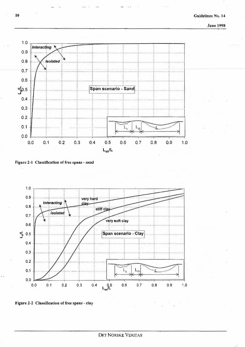
If detailed information is not available Figure 2-1 or figure 2-2 may be used to classify the spans into isolated or interacting dependent on the soil types and span and support lengths. The figures are in a narrow sense only valid for the vertical (in-line) dynamic response but may also be used for assessment of the horizontal (cross-flow) response. In this case the effective lateral soil stiffuess should be used to select the appropriate curve.
• Two or more consecutive free spans are considered to be isolated (i.e. single span) if the static and dynamic behaviour are unaffected by neighbouring spans.
• A sequence of free spans is interacting (i.e. multispanning) if the static and dynamic behaviour is affected by the presence of neighbouring spans. If the free span is interacting, more than one span must be included in the pipe/seabed model.
2.2.2
The morphological classification should in general be detennined based on detailed static and dynamic analyses. The classification may be useful for evaluation of scour induced free spans or in deriving approximate response quantities.
DETNORSKE VERITAS
10
1.0 ·c---:----:-:--=:::::;:=~=--:--:---:--:--:----, lnterac~ng .
0.9
0.8
0.7
0.6
. . . . ............... ·i .. .. ... .... .;. .............. ; ......... .. .. . ; ....... . .... .. : ........... . ... ........ : ............... . ; .............. . . . . . . . . . . . . . . . . . .... ·······:············...:-····· ...... . .
. . . . . .
T- .. . : ······:: T :· : : :·;:· :::~:.:::.:· ... . .... : .. :r.:.· ···-r::· ::·:::: .. . ..... . • ' o I f
~.5 ........... ~ .......... ) .......... ) ......... 1span scenario - Sandi) ......... .) ...................... . ...J
0.4
0.3
0.2
0.1
: : : • . ' . : ! • • • • • ' + . . . . . ' . o o I o o I I
. ....... ·-r···••oo••···~········ .. ··r· ......... r············r-········· ·-1 .. ··········1 ............ 1 .. ······· o I o t o
···········?··--·-······~······ .. ····r··········--~-- .. --··-· ·--:··-······ ~--······-···-~---·-·-·· ---~-·-····· .. . . . . . . . . . . t I ' o o . . .
···········~ ········--·:·············:-············:···---·-····
. : : ·( ) ·( )·(
· ......... ~ ...... --- l .. .) .......... ) ........... -;10::---.......... --::'"'L~·· ~I Ls~hl ~~ 0.0 -1-~~;._.~~~~__;,_.: ~~~:~~-!;::====::;=============;=======;:=====(
0.0 0.1 0.2 0.3 0.4 0.6 0.7 0.8 0.9 1.0
Figure 2-1 Classification of free spans - sand
0.9 r · v~ry h~rtl-··-··· ; ······ ..
0.8 ' .
i 0.7
. . . .: .......... : ............ ~. ········ . . . . . . . . . . . . . . . . . . .... ·:· ···········! ... ·· ······. ··t· ...... 0.6 . . . . . . .
~ 0.5 .J
..... + ... -jsp~n scen~rio - Cl.ay j ..... .J.- ........ + ........ . . . . . . . o o ' I o I t o I o o I ····t···-···-··· ~· ......... '-~ ···········1· ..... .. .. ··;···-········! ............... . 0.4 . - ........ ,.:... .. . .. . .. .. .. . . ~. . . .. .. . . . . . 0 o I I t t
I o o ' o j I f o I o I "'
0.3 ...... ···---~······· .. -~· .. ····· ····f ············~··········--~---······· - ~·-·· ···· ···-~·-·········-~ · -··········~·-····· : : : : : : : : i
0.2 . ········--~--·· o.•···l·· ········+···········+········· -.....,_-~~----:-~ . • I "" ....... L ... a • .-" I L..hl °''~ ... ·: ·········-'"!······ ..... ..
( )( )( 0.1
0.0 0.0 0.1 0.2 0.3 0.4 0.6 0.7 0.8 0.9 1.0
Figure 2-2 Classification of free spans - clay
DET NORSKE VERIT AS
Guidelines No. 14
June 1998
Guidelines No. 14
June 1998
2.3 Temporal classification
Z.3.1
The temporal criterion categorises the free span according to scour or unevenness induced free spans, i.e.
• Scour induced free spans are caused by seabed erosion or bed-form activities. The free span scenarios (span length, gap ratio etc.) may change with time.
• Unevenness induced free spans are caused by an irregular seabed profile. Normally the free span scenario is time invariant unless the operational parameters such as pressure and temperature change significantly.
2.3.2
The free span analysis shall take due account of the temporal classification in the application of the load sequence for the functional loads:
• Scour induced free spans: all loads may be applied in one step.
• Unevenness induced free spans: loading sequence in steps, see section 3.
2.3.3
In case of scour induced spans, where no detailed infonnation is available on the maximum expected span length, gap ratio and exposure time, the following apply:
• Where unifonn conditions exist and no large-scale mobile bed-fonns are present the maximum span length may be taken as the length resulting in a statically mid span deflection equal to one external diameter (including any coating).
• The exposure time may be taken as the remaining operational lifetime or the time duration until possible intervention works will take place. All previous damage accumulation must be included.
2.3.4
Additional information (e.g. free span length, gap ratio, natural frequencies) from surveys combined with an inspection strategy may be used to qualify scour induced free spans. These aspects are not covered herein. Guidance may be found in Fyrileiv et al., (1998).
3. Free Span Analysis
3.1 General
3.1.1
The following tasks normally have to be performed in the assessment of free spans:
• structural modelling • load modelling • a static analysis to obtain the static configuration of the
pipeline
11
• an eigenvalue analysis which provides natural frequencies and corresponding modal shapes for the inline and cross-flow vibrations of the free spans
• a response analysis using a response model or a force model in order to obtain the stress ranges from envirorunental actions.
3.2 Structural modelling
3.2.1
The structural behaviour of the pipeline shall be evaluated by modelling the pipeline, the seabed and relevant artificial supports and perfonning static and dynamic analyses. lo this section requirements to the structural modelling are given.
Soil-pipe interactions are treated in section 4.2.
3.2.2 A realistic characterisation of the cross-sectional behaviour of a pipeline can be based on the following assumptions:
• The pipe cross-sections remain circular and plane. • The two dimensional state of stress (axial and hoop)
should be considered. • The stresses may be assumed constant across the pipe
wall thickness. • A plasticity model based on the von Mises criterion and
associated flow rule may be adopted. • The internal pressure affects the bending response if
yielding takes place • Load effect calculation is normally to be performed
using nominal un-corroded cross section values.
3.2.3
The pressure differential causes hoop stresses to develop in the pipeline wall along with axial stresses. In case of yielding this bi-axial state of stress shall be represented in a consistent way to allow for a realistic cross-sectional behaviour. In particular the influence of the hoop stress and Poisson's effect on the bending stiffness must be considered.
3.2.4
The effect of coating is generally limited to increasing submerged weight, drag forces, added mass and buoyancy. The positive effect on the stiffness and strength is normally to be disregarded. If the contribution of the coating to the structural response is considered significant, appropriate models shall be used.
3.2.5 Non-homogeneity of the bending stiffness along the pipe, due to discontinuities of the coating across field joints or other effects, may imply strain concentrations that shall be taken into account.
3.2.6
The boundary conditions at the ends of the pipeline section modelled shall be able to simulate the pipe-soil interaction and the continuity of the whole pipeline length.
DET NORSKE VERITAS
l2
3.2.7
The element length to be used in a finite element model is dictated by the accuracy required. Typically an element length of I.120 (L is the span length) is sufficient.
3.3 Loads
3.3.1
The loads to be considered for fatigue analysis of free spanning pipelines includes:
• functional loads • environmental loads, comprising
direct loads from wave and current loads induced by hydro-elastic phenomena.
Fatigue loads from trawl impact, cyclic loads during installation or pressure variations are not considered herein but must be considered as a part of the integrated fatigue damage assessment.
3.3.2 The functional loads which shall be considered are:
• weight of the pipe and internal fluid • external and internal fluid pressure • soil pressure if the pipe is locaJJy buried • thennal expansion and contraction • installation forces.
3.3.3
Weight must account for the weight of the pipe considering coating and all attachments to the pipe, the weight of the internal fluid and the buoyancy.
3.3.4 Soil pressure, if the pipe is locally buried, is normally not considered explicitly in the free span analyses but rather implicitly by imposing appropriate soil restraints.
3.3.5
Thennal expansion and contraction loads and possible other changes in pipe behaviour caused by temperature differences shall be accounted for.
3.3.6
Installation forces are to include all forces acting on the pipe during installation . Typical installation forces are applied tension during laying and forces from the trenching machine if trenching is carried out after laying. Pre-stressing such as pennanent curvature or a permanent elongation introduced during installation must also be taken into account.
3.3.7
Response calculations must account for the relevant sequence of load application if important.
Guidelines No. 14
3.4 Static analysis
3.4.1
June 1998
The static configuration is to be detennined for different conditions:
• as-laid condition • flooded condition • pressure test condition • operating condition.
3.4.2
The static analysis should normally account for non-linear effects such as:
• large displacements (geometric non·linearity) • soil non·linear response • non-linear behaviour of the pipe cross-section • loading sequence.
3.4.3
The stiffuess of the pipeline consists of material stiffness plus geometrical stiffness. The effective axial force, Serf, shall be used to calculate the geometrical stiffness. This force is the true steel wall axial force, Nir, with corrections for the effect of external and internal pressures:
Where p; and Pe denotes the internal and external pressure, respectively and Ai and Ae are the corresponding cross· section areas.
For a completely unrestrained (axially) pipe the effective axial force becomes:
For a totally restrained pipe the following effective axial force apply:
where:
ti.T
3.4.4
effective lay tension
internal pressure difference relative to laying, see Rules for Pipelines
pipe steel cross section area
temperature difference relative to laying
temperature expansion coefficient.
The static environmental loads are in this guideline confined to those from on bottom current. The load may be disregarded in the analysis if much smaller than the vertical
DETNORSKE VERITAS
Guidelines No. 14
June 1998
functional loads. However, for light pipes it should be considered.
3.5 Eigen-value analyses
3.5.l The aim of the eigen-value analyses is to calculate the natural frequencies and corresponding mode shapes. In general the analysis is complex and depends on
• the temporal criterion • the pipeline condition (i.e. as-laid, water-filled, pressure
test and operation) • the pipe and soil properties • the seabed classification, effective free span length and
boundary conditions • the effective axial force and the initial deflected shape
after laying • the loading history and axial displacement ("feed-in") of
the pipe.
Jn general, it is recommended to assess the response quantities using non-linear FE-analyses conducted over an appropriate stretch of the pipeline. However, approximate response quantities may be applied in some cases, see section 3.7.
3.5.2
Using a FE-approach, the following comments apply:
• The eigenvalue analysis shall account for the static equilibrium configuration.
• In the eigenvalue analysis, a consistent linearisation of the problem must be made.
• The pipe-soil linearisation should be validated. • The effect of geometric non-linearity on the dynamic
response should be assessed. • The pipe support points may be assumed not to change
during Vortex-Induced Vibrations (VIV).
3.5.3
For a multi-spanning scenario, special care must be paid to the determination of the eigenvalues and associated eigenvectors due to the potential occurrence of very close eigenvalues, especially as concerns the identification of con-ect eigenvectors.
3.5.4
The stress ranges are derived from the mode shapes. The accuracy of the stress ranges is strongly affected by the fmite
13
element modelling. Thus, the element lengths must be short enough to ensure a sufficient number of elements over the free spans that are to be assessed.
3.6 Damping
3.6.l
Response amplitudes are affected by damping. The stability parameter, Ks, representing the damping for a given modal shape is given by:
where:
p
(psfp)
3.6.2
water density
total modal damping ratio at a given vibration mode comprising:
• structural damping, (m, see 3.6.4 • soil damping, Ssoih see 3.6.5 • hydrodynamic damping, Sh, see 3.6.6
specific mass (without added mass)
added mass coefficient.
The effective mass, m , is defined by e
m - ~L'--= _ _ _
[ Jm(s)~2 (s)dsl
e- J~2 (s)ds L
m(s) is the mass per unit length including structural mass, added mass and mass of internal fluid.
3.6.3
The added mass coefficient, Ca, as function of the gap ratio (e/D) is given by Figure 3-1. It applies for both smooth and rough pipe surfaces.
DETNORSKE VERITAS

14
2.00 ·- ......... ·: ......... ··: .................................... ··;· .......... ··1· ······ ····1········· ·; . . . . . . . . . . .
.... .... ~ ...... ·--- ---------- ·:····-······:·-·-·-·-·· ........... ···········:···········:···········:····· ······: l.90 ' . . . . . . . .. . . . ' . . . . . . . ' . . ................................ ............... ............................. ··········~······ ..... ...................... ~ .. .. 1.80 . . . . . . . ' ' ' ' ' ' ' ' . ' . ' ' . . . . ................. ! ............. :··········· ................... ·····:···········1···········1· ---·-····1
~ ~ ~ t ' ... ·····1··········· .......... : ........... : ........... : ... ...... ··········t· ........ t ....... ·1··--···· .. ·1 ... ·- ----- -··: ........ -·-. ! ... -- -- .... ;- .......•. ·······-- -·~- ...... -..... ~- ......... ;· ........... ~
' . . . ' . . ' ' . . . . ' . . ' . . . . . ' ····················-··· .............. . ......... . ................ ... ....... ... ... .. ......... ~-······· ' . . . . . .
.. u 1.70 .... Q Q,l ·o 1.60 e 4J 0
1.50 u "' "' = 1.40 ~ . . . ' ' . . . .
• • t • . . ' . ' ' ' t I ' '
········ ! ········· ··T···· :· : T ·: :::: :.:.:. ··;· : ::r:· :.L· . "" 4J l.30 "O
~ 1.20
. . . . . ' . . . ·····-··•·i·········-· ~ . .. ..... ········ ···~ ········ ••! ··········-~·· · ·······---~ 1.10
1.00
0 0.2 0.4 0.6 0.8 1.2 l.4 1.6 1.8 2
Gap Ratio (e/D)
Figure 3-1 Added mass coefficient versus gap ratio
3.6.4 Structural damping is due to internal friction forces of the pipe material and depends on the strain level and associated deflections. If no information is available, a structural modal damping ratio of
Sstr == 0.005
<'.;, pDC 0 C L-L~l
[
jU(s)cjl2(s)ds ]
h = \jl 4rrf0
- L-=-J m-(s-)$-2-(s-)-ds-
where:
Guidelines No. 14
June 1998
can be assumed. If concrete coating is present, the sliding at the interface between concrete and corrosion coating may further increase the damping to typically 0.01-0.02.
constant to be taken a:> 1.0 for in-line VIV and 0.5 for cross-flow VIV.
3.6.5
For screening purposes the following soil (modal) damping ratio can be assumed:
~I =0.01
For a more detailed analysis, see 4.2.
3.6.6
For VIV the hydrodynamic modal damping ratio ~.,is normally to be taken as zero, i.e.
For VIV the hydrodynamic damping, ~11, is the damping outside the lock-in region for the pipe. The contribution to hydrodynamic damping within the lock-in region shall be set to zero. Thus, ~h. may be taken from:
p
D
Co
fo
water density
outer pipe diameter (including any coating)
drag coefficient
natural frequency
lj>(s) mode shape
U(s)
m(s)
L
Ls
mean flow velocity normal to the pipe as a function of the pipe axis co-ordinate, s.
mass per Wlit length incl. structural mass, added mass and mass of internal tluid
free span length
span length with vortex shedding loads.
~his not to exceed 0.05.
DET NORSKE VERIT AS
Guidelines No. 14
June 1998
3.7 Approximate response quantities
3.7.1
The approximate response quantities specified in this section may be applied for free span assessment provided:
• conservative assumptions are applied with respect to boundary conditions, span length, effective axial force, etc.
• a sensitivity study is perfonned in order to quantify the criticality of the assumptions.
Approximate response quantities are considered relevant in performing efficient screening of FE or survey results in order to identify critical spans to be assessed with methods that are more accurate, see Fyrileiv & M0rk, (1998).
3.7.2
The fundamental natural frequency may be approximated by, see Bruschi & Vitali, (1991):
where:
E
I
M.
Q
Youngs modulus
moment of inertia
effective span length, see 3.7.4
effective mass, see 3.6.2
steel outer diameter of pipe
deflection load per unit length (submerged weight for cross-flow or static current loading for in-line)
s.rr effective axial force, see section 3.4.3
Euler buckling load"" n2EIIL2.rr.
3.7.3
The coefficients Ci. Cz and C3 are given in the table below for different idealised boundary conditions:
Boundary Condition C1 C2 C3
Pinned - Pinned 1.57 J.00 5.0 10·4 ~ 5.0 10·3
Pinned - Fixed 2.45 0.50 5.0 10·5 ~ 5.0 10·4
Fixed - Fixed 3.56 0.25 5.0 10"6 ~ 5.0 10-5
The coefficients C1 and C2 relate to the bending stiffness tenn and axial force tenn in section 3.7.2, respectively. They are theoretically correct for a rectilinear pipe while C3 is an
15
approximate coefficient related to the deflection (sagging) tenn. The higher value for C3 typically apply to as-laid condition and the lower to cases with significant feed-in e.g. during operation.
If more detailed infonnation is not available the following values are recommended:
C1~2.0, C2""0.50, C3,..J.0 10·4
C,,.,2.0, Cr:::0.50, C3,.,5.0 10·5
for as-laid condition.
for in-service condition.
The approximate equation for fo normally predicts frequencies within+/- 30% of the true natural frequency provided (C2 S.ffl'PE) > -0.5 and (LID) < 200.
3.7.4
The ratio between the effective span length, Leff, and apparent (visual) span length, L, depend on the soil and support conditions. If more detailed infonnation is not available it may be taken as:
L.;:r = 1.1 2-0.00{~ -40) 40 <UD< l60 {
1.12 LID < 40
1.0 L/D> l60
3.7.5
The unit diameter stress amplitude (stress due to unit outer diameter mode shape deflection) may be calculated by
where ~(s) is the assumed mode shape satisfying the boundary conditions, D is the outer pipe diameter (including any coating) and 0 5 is the steel pipe diameter. K is the curvature of the mode shape ~(s) at the point (s, ~(s)) to be calculated as ·
2 [ 2)-312 K(s) = .£...1 I+ (ap)
Bs2 Os
Alternatively, SA-io, can be calculated as the quasi-static
stress introduced by the inertia load m(s)~(s)(2nf0r.
3.7.6
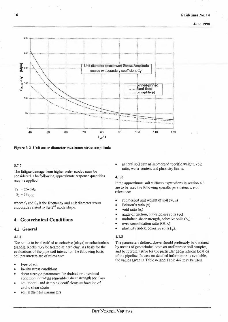
Jf detailed infonnation is not available, the (unit diameter) stress amplitude SA=ID may be taken from Figure 3-2 below. The figure provides SA=ID divided by the boundary coefficient C1 squared. Consistent boundary conditions for evaluation of f0 and SA=ID must be applied.
DET NORSKE VERIT AS
16 Guidelines No. 14
300 ·•••••••·•·•·•· ···········---,······································ ······················· ··· ········· ······ · , ••..••..••••••. . : : : : : . . . . . . . . . . . . . . . . 250 .............. ··········· · ···1··
. . . . . ··········:--··············~···············:············ ··1·············-·r··············
'iO Cl. 200 !.
\ \ ... , ..... .. . .............. , ............... . nt ame er max mum ress Ampll u e
scaled wrt boundary coefficient C1 2
N
~
\ \
' \ \
\ 0 150 ' . .. , • • •• __________ _.1 ........ - .. . -. :·-···---------·-: .. ···········-:·--r-----.---.--..--'-r-. .. ·. .. ..
\. : . , : ' ' ' : '' . . ' .... .
100 ......... : · ....... : ···--------~~---·· ·:·.. : .............
I o, I
. . --ptnne -ptnn · · . -... fixed .. fixed
- - - pinned-fixed . ' . . . .. .................................. ,, ....................... . . . . . . . . .
~ . ··- ... : '11.... .....
50 ....•..•.•..... ; ....•...••. .•• )::.-:.:::: . •.• -~.·: ·-~-~-~~~+ .. :":----- --.... · - -- ~·-·· -- -:-. ______ _ ... . .. .. .. ; ... .
. ........ .. ·: ........... .. ' ... ; ..... -: .~.- -
O +----~---~---.-;-----:-----::-----:-----:------l
40 50 60 70 90 100 110 120
Figure 3-2 Unit outer diameter maximum stress amplitude
June 1998
3.7.7 The fatigue damage from higher order modes must be considered. The following approximate response quantities may be applied:
• general soil data as submerged specific weight, void ratio, water content and plasticity limits.
f2 = (2-3)f0
S2 = 2SA=ID
where f2 and S2 is the frequency aud w1it diameter stress amplitude related to the 2"" mode shape.
4. Geotechnical Conditions
4.1 General
4.1.1
The soil is to be classified as cohesive (clays) or cohesion less (sands). Rocks may be treated as hard clay. As basis for the evaluations of the pipe-soil interaction the following basic soil parameters are ofrelevance:
• type of soil • in-situ stress conditions • shear strength parameters for drained or undrained
condition including remoulded shear strength for clays • soil moduli and damping coefficients as function of
cyclic shear strain • soil settlement parameters
4.1.2
If the approximate soil stiffness expressions in section 4.3 are to be used the following specific parameters are of relevance:
• submerged unit weight of soil ( w soit)
• Poisson's ratio (v) • void ratio ( e5)
• angle of friction, cohesionless soils ( q>5)
• undrained shear strength, cohesive soils (Su) • over-consolidation ratio (OCR) • plasticity index, cohesive soils (ip).
4.1.3
The parameters defined above should preferably be obtained by means of geotechnica\ tests on undisturbed soil samples, and be representative for the particular geographical location of the pipeline. In · case 110 detailed infonnation is available, the values given in Table 4-land Table 4-2 may be used.
DETNORSKE VERITAS

Guidelines No. 14
June 1998
Soil type <p. Wsoil
[kN/m3]
v es
Loose 30° 9.1 0.35 0.7
Medium 35" 9.6 0.35 0.5
Dense 40° 10. J 0.35 0.4
Table 4-1 Typical gcotech mcal parameters for sandy soils
Soil type Cu Wsoil v es Ip
[kN/m3] [kN/m3
] l%J
Very soft 5 4.4 0.45 2.0 60
Soft 17 5.4 0.45 1.8 55
Stiff 70 7.4 0.45 J.3 35
Hard 280 9.4 0.45 0.8 20
Table 4-2 Typical gcotechnical parameters for clay (OCR=l).
4.1.4
The uncertainties in the soil data should be co11sidered. lt may arise from variations in soil conditions along the pipeline route and difficulties in detennining reliable in-situ soil characteristics of the upper soil layer, say, 0.02-0.05 m for small diameter pipelines to 0.2-0.5 m for large diameter pipelines.
4.2 Modelling of soil interaction
4.2.1
The pipe-soil interaction is important in the evaluation of the static equilibrium configuration and the dynamic response of a free spanning pipeline. The following functional requirements apply for the modelling of soil resistance:
• The seabed topography along the pipeline route must be represented.
• The modelling of soil resistance must account for nonlinear contact forces nonnal to the pipeline and lift off.
• The modelling of soil resistance must account for sliding in the axial direction. For force models this also applies in the lateral direction.
• Appropriate (different) short- and long-tenn characteristics for stiffness and damping shall be applied, i.e. static and dynamic stiffiless and damping.
4.2.2
The seabed topography may be defined by a vertical profile along the pipeline route. The spacing of the data points characterising t11e profile should relate to the actual roughness of the seabed.
17
4.2.3
The axial and lateral frictional coefficients between the pipe and the seabed shall reflect the actual seabed condition, the roughness, the pipe, and the passive soil resistance.
4.2.4
The axial and lateral resistance is not always of a pure frictional type. Rapid changes in vertical stresses are (in low permeable soil) reacted by pore water and not by a change in effective contact sh·csses between the soil and the pipe. In addition, the lateral resistance will have a contribution due to the penetration of the pipe into the soil, which need to be accounted for.
4.2.5
For sands with low content of fines, the frictional component may be proportional to the vertical force at any time, whereas for clays the 'frictional' component is more related to the static vertical force for which the clay is consolidated.
4.2.6 Where linear soil stiffness have to be defined for the eigenvalue analysis, the soil stiffness should be selected conside1i11g the actual soil resistance and the amplitude of the oscillations.
4.2.7
The soil stiffness for vertical loading should be evaluated differently for static and dynamic analyses. The static soil response will mainly be governed by the maximum reaction, including some cyclic effects. Dynamic stiffness will mainly be characterised by the unloading/re-loading situation.
4.l.8 The soil damping is generally dependent on the dynamic loads acting on the soil. Two different types of soil damping mechanisms can be distinguished:
• Material damping associated with hysteresis taking place close to the yield zone in contact with the pipe.
• Radiation damping associated with propagation of elastic waves through the yield zone.
4.2.9
The material damping is dependent on the relative stress level in the soil, which again depends on the amplitude of the pipeline oscillations at the contact points with the soil. The contribution of material damping is more important for inline VIV than for cross-flow VIV, since in-line sliding between pipe and soil may give larg~ hysteresis effects.
4.2.10
The radiation damping may be evaluated from available solutions for elastic soils using relevant soil modulus reflecting the soil stress (or strain) levels. The radiation damping depends highly on the frequency of the oscillations, and is more important for high frequency oscillations.
DETNORSKE VERITAS
18
4.2.11
The modal soil damping ratio, ~oil> due to the soil-pipe interaction may be determined by:
where the soil damping per unit length, c(s), may be defined on the basis of an energy balance between the maximum elastic energy stored by the soil during an oscillation cycle and the energy dissipated by a viscous damper in the same cycle.
Alternatively, the modal soil damping ratio, ~oii. may be taken from Table 4-4 and Table 4-3. Interpolation is allowed.
LID Clay Sand
Soft Medium Hard Loose Medium Dense
< 40 5.0 2.0 1.4 3.0 1.5 1.5
100 3.5 1.4 1.0 2.0 1.5 1.5
> 160 2.0 0.8 0.6 1.0 1.5 1.5
Table 4-3 Modal soil damping ratios in[%). Horizontal (in-line) direction
LID Clay Sand
Soft Medium Hard Loose Medium Dense
< 40 3.0 1.2 0.7 2.0 1.2
JOO 2.0 1.0 0.6 1.4 1.0
> 160 1.0 0.8 0.5 0.8 0.8
Table 4-4 Modal soil damping ratios in[%]. Vertical (cross-flow) direction
1.2
l.O
0.8
Guidelines No. l4
June 1998
4.2.12
It should be emphasised that the determination of pipeline/soil interaction effects is encumbered with relatively large uncertainties stemming from the basic soil parameters and physical models. It is thus important that a sensitivity study is performed to investigate the effect of abovementioned uncertainties.
4,3 Approximate Soil Stiffness
4.3.1
The following expressions may be llScd for the static, vertical soil reaction per unit length as a function of the settlement, v:
where
b {2J(D - v)v forv 5 0.5 D D forv >0.5D
D outer pipe diameter (including any coating)
W 50n submerged unit weight of soil
Su undrained shear strength.
4.3.2
The bearing capacity factors Ne. N~ and N.1 versus internal friction angle cp., may be taken from Figure 4-1. For clayey soils the friction angle is set equal to O", i.e. N,
1 = 1.0 and
N0 =-= 5.l4.
DETNORSKE VERJTAS

Guidelines No. 14
June 1998
100 ~~~~~~~~~~~~~~~~~~~~··~~~ ···!· .. -:-··"···1·· ·•i .. .. ;. .... :.. •.. : .•.•...•
z .... 'C c Ill 10
D" z 0 z
1
0
•• •:• • • ·:• • •i••• i••• • • ·t · • ·f • • •j••., ~o • • o • •1•• • I 1 I ' ............. ...... ................. ,.. ... ,. .. ~-·· .. ............. ..... ............ .... .. . . ··~---·~···~- - -~··· ···!··-~··+ · .. ~··· ··-~··· ···~··+-·· ···l···i· .. -: .. ' ' ' . · ·1·4
• ·;-·· ~- • • ~- • • • • ·f ···r 0 ·1· ·· ~- · · · ·· ~ -·· · ·-r · --~------T · -~ - · · ·; ~- · · · ~---·(- -~·- -1··--- -:- ---:----:--·..f··· · · ·t···!- · ··!····'· · · ··-~··· ··-~--·;.-- - ·-;-- ..... - ·-. ···:---·:·-·-:·--~·-· : : : : : : : : : : : : . : ; : : : ·rr-r-r· ... ~···; · r ·-· · · ·1 · · ·r .. : ..... ; · · 1· ·!· · ... \ · i ... r·r ·· · ·r·r~·-· ... =···r r .. ?··· ...... T -r·:--·
' ..
10 20
. ... .... . . . . .... ' o o I
. .. . ........ ....... ..-.... _ ....... ..
. ... . . . . . .. . . . . . . .. . ..... .. ·· ·········· ... ,. ........ , ........ . . . . . .. . . . . .. . . . .. I • I ' ' . . . .. . . . .. . . . .. . . .. . . .. . . .. . . ..
30 40 50
<p[degreeJ
Figure 4-1 Bearing capacity factors N0, Nq and N1 versus the internal friction angle <p1
4.3.3 4.3.4
The ma.'<imum static, axial soil reaction per unit length may be taken as:
The dynamic soil stiffness in the vertical and horizontal (lateral) direction may be taken as:
- clayey soils: R ~ = min~ ~µ8 , bT max }
where: where:
Rvs vertical static soil reaction given by 4.3. l.
axial friction coefficient
G b given in section 4.3 . l
K = 0.88-G v 1-v
K1 =0.76 ·G·(l+v)
I + e $
{
1955-(2.97 -e,)2 .Jcr:
1300 ·(2.97-e,\2
,fci;(OCR)k, I +e,
sand
clay
19
{kN/m2
s~ -( O.S(l -bk,)R: )' is lhe soil shear strenglh effective soil stress in [kN/rn2] to be calculated as:
cr,= 0.75 WsoH b where b is given in section 4.3.1.
..fOCR(1-~)+(~) 2.61 200 200
OCR over-consolidation ratio
void ratio
The coefficient ks, may be taken from Figure 4-2.
D ET NORSKE VERIT AS

20
05
""'"' v _,./
/ 04
/ v
/ 7
,.V 0.3
~
/ "' 02
/ v -
,v v 01
/
0 v 0 20 60
Plasticity index, ip
Figure 4-2 k. versus plasticity index, ip
4.3.5
lfno information is available on the dynamic axial soil stiffness, it may be taken equal to the dynamic lateral soil stiffness as described above.
4.4 Artificial supports
4.4.J
Gravel sleepers can be modelled by modifying the seabed profile, considering the rock dump support shape and applying appropriate stiffness and damping characteristics.
4.4.2
The purpose of mechanical supports is generally to impose locally a pipeline configuration in the vertical and/or transverse directions. Such supports can be modelled by concentrated springs having a defi ned stiffness, taking into account the soil defonnation beneath the support and disregarding the damping effect.
5. Hydrodynamic Description
5.1 Flow regimes
5.1.1
The current flow velocity ratio, a=UJ<Uc+Uw}. see 5.2.6, may be applied to classify the flow regimes as follows:
i--........ -
80
CL< 0.5
0.5 <a < 0.8
DETNORSKE V ERITAS
Guidelines No. 14
June 1998
-
- 1-- 1--
100 120
wave dominant - wave superimposed by current.
ln-line direct ion: in-line loads may be described according to Morison's formulae, see section 9.2. In-line VIV due to vortex shedding is negligible.
Cross-flow direction: cross-flow loads are mainly due to asymmetric vo1tex shedding. A response model, see section 8.3, is recommended. Alternatively a force model may be applied, see section 9.3.
wave dominant- current superimposed by wave
In-line direction: in-line loads may be described according to Morison's formulae, see section 9.2. In-line VIV due to vortex shedding is negligible.
Cross-flow direction : cross-flow loads are mainly due to asymmetric vortex shedding and resemble the cu1Tent dominated situation. A response model, see section 8.3, is recommended. Alternatively a for~ model may be applied, see section 9 .3.

Guidelines No. 14
June 1998
a.> 0.8 current dominant
In-line direction: in-line loads comprises the following components :
a steady drag dominated component
a oscillatory component due to regular vortex shedding
For fatigue analyses a response model applies, see section 8.2. In-line loads according to Morison's formulae may, however, still be present.
Cross-flow direction: cross-flow loads are cyclic and due to vortex shedding and resembles the pure current situation. A response model, see section 8.3, is recommended. Alternatively a force model may be applied, see section 9.3.
Note that a=O correspond to pure oscillatory flow due to waves and a.=l correspond to pure (steady) current flow.
The flow regimes are illustrated in Figure 5-l.
21
6 ••••••••••••• •••• ··-·· •••••••• ··-········ · ••••• .•••••••••••••••..•.••••. ••• • •••• ••.••••••••••••••••••••
······1r-··--·······t··· .............. ·t ·····;···-····:: .. • • •• •• •• • current dominated • • • • '•.
' ' , ' 4 : ••••••••••••••••••••• ••• ,.tl.QW .......... .... .. / ·· ·· ·· ·· ······ ········ .. .-.. .................... ... ' , ,,.,,,,. " ,
wave dominated llow ' •,. . ,• • J a=-0.s J~ ,,. · . ._ .. ·' +······················ + .... : .... -,<.'. ....... ..... .............. ........ . . ·'" ~· · •<. ....... .
·1 ··········· ·····-············ ••. time
· 2 ............. . . ................. ... ............ .............................. ........... .
Figure 5-l Flow regimes
5.1.2
Oscillatory flow due to waves is stochastic in nature, and a random sequence of wave heights and associated wave. . periods generate a random sequence of near seabed orbital oscillations. The following definition oftl1e wave induced flow velocity amplitude, Uw, applies:
• In case of a fatigue analysis based on decomposition of sea states into single random waves, Uw corresponds to each single velocity amplitude at pipe level.
• In case of a fatigue analysis based on characteristic harmonic oscillation representing an entire sea state the characteristic velocity amplitude, Uw *, applies, see section 6.3.
DET NORSKE VERIT AS
22
5.2 Hydrodynamic parameters
5.2.1
Vortex induced vibrations (VIV) and direct wave actions are affected by several parameters, such as:
• Reynolds number, Re • Strouhal number, S1
• reduced velocity, VR • Keulegan-Carpenter number, KC • current flow velocity ratio, a • flow angle relative to the pipe. Herein, only the
component normal to the pipe axis is to be considered • pipe roughness, (k/D) • gap ratio (seabed proximity), (e!D).
Herein a brief introduction of the basic hydrodynamic parameters is given. For a thorough introduction see e.g. Sumer & Freds0e, (I 997) and Blevins ( 1994).
5.2.2 Vortex shedding from pipe is a function of Reynolds number:
R = UD e v
where U is the flow velocity, Dis the outer pipe diameter of the pipe (including any coating) and v is the kinematic viscosity ("'='l.5·10·6 [m2/s] ).
5.2.3 The vortex shedding frequency in steady cun·ent or regular wave flow with KC numbers greater than 30 is approximated by:
where fs is the vortex shedding frequency, Uc is the current velocity and Uw the wave induced velocity amplitude normal to the pipe. The Strouhal number, S" is a function of Reynolds number and other parameters.
5.2.4 The reduced velocity, YR, is in the general case with combined current and wave induced flow, defined as:
V _ Uc+Uw R - foD
where f0 is a natural frequency for a given vibration mode.
5.2.5 The Keulegan-Carpenter number, KC, is defined as:
Guidelines No. 14
June 1998
where fw is the wave frequency.
5.2.6
The current flow velocity ratio, a, is defined by:
5.2.7
The pipe roughness influences the boundary layer on the pipe and thereby the vortex shedding. The effect of pipe roughness in t11e range 0.005 < (k/D) < 0.02 is..implicit in the response models.
5.3 Seabed proximity
5.3.l
The gap is defmed as the distance between the pipe and the seabed. The gap used in design, as a single representative value, must be characteristic for the free span
• For in line VIV the gap may be calculated as the average value over the central third of the span.
• For cross-flow VIV, the gap may be taken as the maximum modal pipe deflection (vertical) allowed by the presence of the sea-bottom.
5.3.2 The presence of a fixed boundary near the pipe (proximity effect) has a pronounced effect on the response, e.g.:
• The physics of pipe vibrations close to a boundary (i.e. the seabed) is different from the physics of a vibrating free pipe.
• The alternating vortex shedding is suppressed for small gap ratio (typically for (e/D) < 0.3); however selfexcited vibrations (cross-flow) still take place initiated by fluctuations in the hydrodynamic lift force.
• Significant vertical oscillations exist for (e/D) < l at oscillatory flow conditions (i.e. a < 0.5) with a vibration frequency twice the wave frequency.
• The drag coefficient C0 and inertia coefficient CM increase in the proximity of the boundary.
5.3.3 Details on seabed proximity effect may be found in the literature, (see Sumer & Freds0e, 1997). Herein, the effect of the sea-bed proximity is treated conservatively, i.e.:
• For in-line VIV, any mitigation effect is ignored. • For cross-flow VIV the sea-bed effects (for e/D < 0.5) is
introduced conservatively in t~e Response Model using a simplified approach.
DET NORSKE VERIT AS
Guidelines No. 14
June 1998
6. Environmental Conditions
6.1 General
6.1.1
The objective of the present section is to provide guidance on:
• the long term current velocity distribution • short-term description of wave induced flow velocity
amplitude and period of oscillating flow at the pipe level • long term statistics
to be applied in fatigue assessment in section 7.
6.1.2
The environmental data to be used in the assessment of the long-term distributions shall be representative for the particular geographical location of tl1e pipeline free span.
6.1.3
The fl.ow conditions at the pipe level due to current and wave action gov em the response behaviour of free spanning pipelines. The principles and methods as described in Classification Note No. 30.5 may be used in addition to this Guideline as a basis when establishing the environmental load conditions.
6.1.4
Preferably, the environmental load conditions should be established near the pipeline using measurement data of acceptable quality and duration. The envirorunental data must be collected from periods that are representative for the long-term variation of the wave and current climate, respectively. In case of less reliable or limited number of, wave and current data the statistical uncertainty should be assessed and included in the analysis if significant.
6.1.5
The wave and current characteristics must be transferred (extrapolated) to the free span level and location using appropriate conservative assumptions. The level of the free span is defined relative to the mean water (surface) level (MSL) by the distance from the top of the pipe to the MSL. In case of large free span deflection, the top of the pipe should be taken as the average over the pipe span.
6.2 Current conditions
6.2.1 The steady current flow at the free span level may be a compound of:
• tidal cun-ent • wind induced current • stonn surge induced current • density driven current.
23
6.2.2
When detailed field measurements are not available, the tidal, wind and stonn surge driven current velocity components may be taken from Classification No. 30.5. For current measurements, data analyses and transfo1mations of current characteristics reference is given to the MUL TIS PAN Design Guideline, (1996).
6.2.3
For water depths greater than 100 m the ocean currents can be characterised in tenns of the driving and steering agents:
• The driving agents are tidal forces, pressure gradients due to surface elevation or density changes, wind and sto1m surge forces.
• The steering agents are topography and the rotation of the earth.
The modelling should account adequately for all agents.
6.2.4
The distribution type for the long-term current velocity distribution should be selected based on the physics and experience. Normally a 3-parameter Weibull distribution is considered representative:
where F( •) is the cumulative distribution function. a.c, Pc and Ye are Weibull distribution parameters and U0 is the current velocity.
6.2.5
Directional infonnation of the current velocity may be used in the analysis. If no such infonnation is available, the current should be assumed to act perpendicular to the axis of the pipeline.
6.2.6
The current velocity profile in the boundary layer in areas where flow separation does not occur may be taken as:
where:
V*
K
z
friction velocity
von Kannan's constant ( = 0.4)
elevation above the seabed
reference measurement height
Zo bottom roughness parameter to be taken as:
DET NO RS KE VERIT AS
24
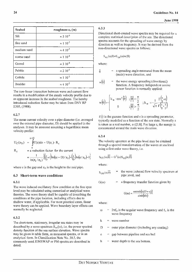
Seabed roughness 7<1 (m)
Silt :::::: 5 10"6
fine sand <::! l 10·5
medium sand ::::: 4 10-s
coarse sand :::::: 1 10·4
Gravel ~ 3 10·4
Pebble -"" 2 10"3
Cobble :::::: I 10·2
Boulder ""'4 10·2
The non-linear interaction between wave and current flow results in a modification of the steady velocity profile due to an apparent increase in the seabed roughness. The hereby introduced reduction factor may be taken from DNV RP E305, (1988).
6.2.7
The mean current velocity over a pipe diameter (i.e. averaged over the external pipe diameter, D) should be applied in the analyses. It may be assessed assuming a logarithmic mean velocity profile:
e+D
Uc(z0 ) = J U(z)dz = U(zr)· Re
e Re = a reduction factor for the current
= 1 {(..:.+1)1n((e + D)!z0}-(..:.)1n(e/ zo}-1}
ln(zr I z0) D D
where e is the gap and z0 is the height to the mid pipe.
6.3 Short-term wave conditions
6.3.1 The wave induced oscillatory flow condition at the free span level may be calculated using numerical or analytical wave theories. The wave theory shall be capable of describing the conditions at the pipe location, including effects due to shallow water, if applicable. For most practical cases, linear wave theory can be applied. Wave boundary layer effects can normally be neglected.
6.3.2 The short-term, stationary, irregular sea states may be described by a wave spectrum S~~(co), i.e. the power spectral density function of the sea surface elevation. Wave spectra may be given in table fo1m, as measured spectra, or in an analytical form. Jn Classification Note No. 30.5, the commonly used JONSWAP or PM spectra are described in detail.
Guidelines No. 14
June 1998
6.3.3
Directional short-crested wave spectra may be required for a complete statistical description of the sea. The directional spectra accounts for the spreading of wave energy by direction as well as frequency. It may be derived from the non-directional wave spectra as follows:
S,1,1 ( (l),O)=S,1,1 (co )w(O)
where:
a spreading angle measured from the mean (main) wave direction, and
the wave energy spreading (directional) function. A frequency independent cosine power function is normally applied:
r(-) is the gamma function ands is a spreading parameter, typically modelled as a function of the sea state. Normally s is lakcn as a real number, SE [2;8]. For larges, the energy is concentrated around the main wave direction.
6.3.4
The vclocily spcchUm at the pipe level may be obtained through a spectral transfonnation of the waves at sea level using a first order wave theory, i.e.
' - 2 -Suu(co,0) = G ((l))S'1 11(<o,0)
where:
Suu (co,6)
G(ro)
where:
k
D
e
h
the wave induced t1ow velocity spet:trum at pipe level, and
a frequency transfer function given by
G(ro) = oocosh{k(D + e)) sinh(kh)
2nfw is the angular wave frequency and t~v is the wave frequency
wave number
outer pipe diameter (including any coating)
gap between pipeline and sea bed
water depth to the sea bottom.
DETNORSKE VERITAS

Guidelines No. 14 25
June 1998
6.3.5 The spectral moments of order n is defined as:
"' M0 = JronSuu(ro)dro
0
• Bandwidth parameter:
f.=~1 - M~ MoM4 The following spectrally derived parameters appear:
• Significant flow velocity amplitude at pipe level:
• Mean zero upcrossing period of oscillating flow at pipe level:
The process (spectrum) is narrow-banded fore~ 0 and broad banded fore ~ l (in practice the process may be considered broad-banded fore larger than 0.6). Us, Tu and e may be taken fromFigure 6-1, Figure 6-2 and Figure 6-3 assuming linear wave theory. In the figures, Tn is a normalisation period and y is the JON SW AP spectrum peakedness parameter.
0.3
~ ~ p 0.2
0.5 .--·~--~····--· --- ·····-···· i ··········· · ··· · ··· · · · · ·· ···:·· · ··· · ··· · ··········· · ··· · ·~·-··························: .. ······ ... ·····················: -~~ ; j i i
~:i... : : : : : ": : : : :
......................... \..l~----·······-········· ·· ··· l ·· · ··· · ··· · ··· · ··· · ··· · · · · · -~·····························=··········· · ··········· ··· ···= ! ~ l : j ! ; ' - : ; ,, : . : '
........ .. ................. ; ............ '!\, ..... -·~ ···························i············· · ··············~·-··· · · · ·····················i
1 ~ '. I = :
: "\, : : . . ......................... , : r=l.0; 3.3; 5.0 rT~-~--·--·-----·--l··· .. .... .. ..... ·-.. ····-y---....................... ,
i ~ : i i
0.4
. . . . . . .................... -·---·---, -------- ---·-·-·-------·- ·--,·-·-·-·-·---·-·-· . . . . . . . . . -... -. -~- ....... -... -... ............ -~·...... . .................... -~ 0.1
. . . . . .
o.o L ___ j_ ___ _J_ ___ _i__=::::::l:::::::::::===d 0.0 0.1 0.2 0.3 0.4 0.5
Figure 6-1 Significant wave induced flow velocity amplitude, Us
DETNORSKE VERrTAS

26 Guidelines No. 14
June 1998
l.S -.. -- .......... -. -·-..... , ........................................ ---·--·· ..... --.... .. -·--· ... . -.......... ·- -...-· -.... .. .... ·---·--· ..... --.. . . . . . . . . . . . . . . . 1.4
1.3 ·······-·············--·1················-·--· ·····r···1 : : ~- ~~~~~~~~
. . ...................... ··:·········· ....... ·········:····· .......... ·········I· 1.2
. .
... ............ ........... ·-~· ..... ...................... . ·-·r .... ···--
.. ,..,. ..-". : _ '/" : o o I ........ ~ -~ -~;·:.:·:;~1 - · · ···················1·························1············· ····-······r··· ········· ···· ·· ·· ···1
,,.,,, : : : : : ··· ·· .. 1 .. ... · -· · ······· · ··· · -··r··-······ ····-· ··· ·· ·· i ·-·· ·· ·· ·· .. ·· · · ··· · · · · · -:-· ... :.r .. ;,;c'hi;;)·o:s .. ·--1 : ; : n ~ :
0.9
0.8
o o 0 I
' + o I
0.7+-~~~~~~+·~~~~~~-+-· ~~~~~~~·,__~~~~~--+~~~~~~-i
0.0 0.1 0.2 0.3 0.4 0.5
Figure 6-l Zero-up-crossing period, T"
0.8 .·. ·. : . . ... ::': .. :· ... ·.:.: ·_] ·_···:···_ ··:··:···: I :·· . . .. .. . . L . ··_ : ·_ . ·1 0.7 . . . . . . . . .
(.I) 0.4
. . . \; l I I I 0
..... .. ... ~-~~·· · .. --·1·· ········ .. -· .. -· .. ······r·························1·················· .. ·····+· ·· ·· ·· · · -· - · -- · -·· · · ·-~ -~, . : -~ .
· · · · •· · · • · · · · · ·· ·r~ '."' · ·· ·· -- -- ·· · · · · - ·-- ··· ~ ·: ·-·· ·· ·· ··· · ·· ·· · · · · ··· · · 1 • • ••• • ••• • •• • • • • • • • • ••• • • -:- • • • • • • • •• • • • • • • • • • • • •• • • -~
·~'\ y=l.0; ,3.3;5.0 I , j ········· ··· ···- · ···--·-{-·, ., . . . .. ··· ·· ···· ·····:--- .......... .. .. .. .. .. . ; ... ............ ................ ; .. ---------- .. -- ...... .... ,.: : Iii'" : : : : : ', ~ : : l
' .
0.6
0.5
0.3
0.2 ~--=-----......... ,.~ .
........ ........_....... I
........... ... ................ ~---········ ·· ·· ·· ··· · ·:- ··--···-··· ···- ···-·· ·--:-· · ··- ·· - · ··· ····-------·:··· · - ~- ...... -.. ;-..;,:
' . 0.1 .. ........ .............. l ... .. ............ · ··· ··-·1--··-··-··-···········l ··-··~-· ··-··-...... (. ·-T~;(higjo.s· ·· ··- · ~
. . ' . . . . . 0+-~~~~~~~·~~~~~~-+~~~~~~-+-' ~~~~~~-t-~~~~~---1·
0.0 0.1 0.2 0.3 0.4 0.5
Figure 6-3 Bandwidth parameter s
DETNORSKE VERITAS
Guidelines No. 14
June 1998
6.3.6 where:
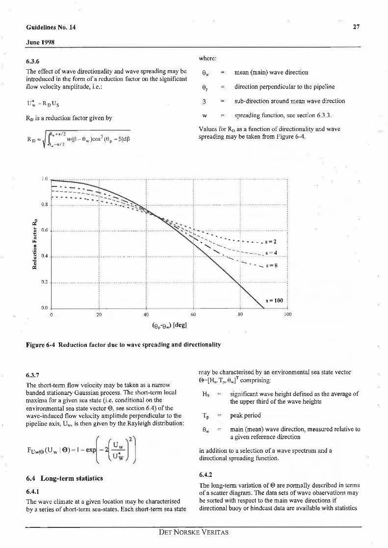
The effect of wave directionality and wave spreading may be introduced in the form of a reduction factor on the significant flow velocity amplitude, i.e.:
mean (main) wave direction
direction perpendicular to the pipeline
sub-direction around mean wave direction
Ro is a reduction factor given by w spreading function, see section 6.3.3.
Values for Ro as a function of directionality and wave spreading may be taken from Figure 6-4.
l.O r-"--·-----·-_ .. _ .. _········-·r ·---· ---·--·-- -- ·--·.l·-·····-···-···-.. ·-· .. r.·············· .. ··- .... !. ···-·······-·-· -_:: .:::.:.:-_::+ .... : : : .. - .. - .. - .. _ - .. ::- -~ ., : : : .
0.8 ---·------· - .. ......... -~ .•. : . :. _., . .. -::;.-t; ... . .. ~--------··· ............... -~· .............. ·------· ; .......... ---... -- -...... ... : ...... --:,~ · '
"'' t . ~ ~ .... ' o ~..... .. I '
::; 0.6 : : " ...... . • :. : ~ -- ........... .. ........... :···············-·--- ···:··-···-···-··· ..... .. ~~~ - ·.:. ·:···· ···········-~--- .......... . C'-1 : ,~ ..... , .................. •' ~ : I , .... , :· • • •• s=2 = : ' ........ , ·~ 0.4 .................... ·-·: ····· ............ ) ....................... f ......... >.~.::;-: .~:~- ~:: .":" . -:-. , .~ .~~ ..... : 1 : : . "":..._ : i:z:: ; ; ··-s=8 : . . . . . . . . . .
0.2 .. -·· .. . . . ... ···· · ·····-~·-···-· --·· ··· · ··· ·· ····~····· · ·-· · ·-··· --·---·--i-- - ·······--· - · ··-·-·· .f ......................... . : . . . . . . . . . . . . . . . . . . s = 100 :
0.0 -1-------1-------1-------1-------l----4.----4
0 20 40 60 80 100
Figure 6-4 Reduction factor due to wave spreading and directionality
6.3.7 may be characterised by an environmental sea state vector E>=(H., Tp, 9w)T comprising:
27
The short-tenn flow velocity may be taken as a narrow banded stationary Gaussian process. The short-term local maxima for a given sea state (i.e. conditional on the environmental sea state vector e, see section 6.4) of the wave-induced flow velocity amplitude perpendicular to the pipeline axis, Uw, is then given by the Rayleigh distribution:
Hs significant wave height defmed as the average of the upper third of the wave heights
6.4 Long-term statistics
6.4.1
The wave climate at a given location may be characterised by a series of short-term sea-states. Each short-term sea state
T P peak period
ew main (mean) wave direction, measured relative to a given reference direction
in addition to a selection of a wave spectrum and a directional spreading function.
6.4.2
The long-tenn variation of e are normally described in terms of a scatter diagram. The data sets of wave observations may be sorted with respect to the main wave directions if directional buoy or hindcast data are available with statistics
DET NORSKE VERIT AS
28
on the observations for different sectors. Otherwise, the statistical properties may be assumed identical for aJI sectors.
In some locations also the joint environmental probability density function providing a continuous representation for e or ranked sets of wave height and associated periods are available.
6.4.3
The fatigue analysis is normally most conveniently performed using a scatter diagram. Thus, the fatigue damage is evaluated in each cell in a scatter diagram in tenns ofHs, Tp and 8w times the probability of occurrence of the (shorttenn) sea-state followed by a summation over all sea-states, see 7.2.5.
6.4.4
Alternatively, the fatigue analysis may be based explicitly on the long-term wave induced flow velocity at the pipe level, see 7 .2.4. In this case, the long-tenn wave induced flow velocity distribution may be derived from a set of stationary short-term sea states:
fuw(Uw)= Jfuwie(Uw 19)dFe
E>
where f Uwl0 ( uw I e) is the conditional short tenn
probability density function for Uw defined by 6.3.7 and Fe is the distribution function for the environmental sea state vector 0, e.g. represented by a scatter diagram or given explicitly by a joint envirorunental probability distribution.
7. Fatigue Analysis
7.1 General
7.1.l
Vibrations due to vortex shedding and direct wave loads.are allowed provided the fatigue criteria specified herein are fulfilled.
7.1.2
The following functional requirements apply:
• The aim of fatigue design is to ensure an adequate safety against fatigue failure within the design life of the pipeline.
• The fatigue analysis should cover a period which is representative for the free span exposure period.
• All stress fluctuations imposed during the entire design life of the pipeline capable of causing fatigue damage shall be accounted for.
• The local fatigue design checks are to be performed at all free spanning pipe sections accowiting for damage contributions from all potential vibration modes related to the actual and neighbouring spans.
Guidelines No. 14
June 1998
7.1.3
The fatigue acceptance criteria in this guideline are based on the interaction free Palrngren-Miners damage rule. The fatigue analysis requires suitable SN-curves for the actual pipe. The SN- curves must be applicable for the material, construction detail, state of stress and corrosive environment
7.'1,4
The concept adopted for the fatigue analysis applies to both response models and force models. The stress ranges to be used may be detennined by:
• a response model, see section 8 • a force model, see section 9.
The stress ranges and natural frequencies should nonually be obtained from a FE-approach. Requirements to the structural modelling and free span analysis are given in section 3.
7 .2 Fatigue criteria
7.2.1
The fatigue damage assessment is to be based on the accumulation law by Palmgren-Mincr:
where:
Drai accumulated fatigue damage
Tl a llowable damage ratio
~ = summation over all stress fluctuations in the design life.
7.2.2
Ni is the number of cycles to failure at stress range S; defined by the SN curve (see section 7.3):
where:
m fatigue exponent (the inverse slope of the SN curve)
C characteristic fatigue strength constant.
7.2.3
ni is the number of cycles corresponding to the stress range S; given by:
where:
DETNORSKE VERITAS

Guidelines No. 14
June 1998
7.2.4
probability of a given flow condition
dominating vibration frequency of the considered pipe response
time of exposure to fatigue load effects (i.e. design life).
When several potential vibration modes may become active simultaneously at a given current velocity the mode associated with the largest contribution to the fatigue damage must be applied. Formally, the fatigue damage criteria may be assessed numerically as:
where:
A
S(A)
F,.. (A)
7.2.5
vector of environmental parameters. In the response model approach it comprises the non-dimensional hydrodynamic parameters: A=(VR, KC, o:)
stress range for a given outcome of A
long tenn probability distribution (vector-) function for A, e.g. derived from section 6.2 and 6.4.
For practical applications the following approximate fatigue damage criterion applicable to both in-line and cross-flow VIV is recommended:
00
Dra1 = T~e · L Pr(•) Jmax(rvs(v~;cx• ; Kc•f }Fuc ~11 H,,Tp,9w O
where
s
probability of occurrence for the given sea-state (Hs, Tp, 9w)·
stress range determined from the response models given in section 8.
dominating vibration frequency to be taken as (response model):
fv= 2fw: for (KC< 5) or gap ratio (e/D) < 0.3
fv = f0,c,: vortex induced cross-flow motion
fv= fo,cr: cross-flow induced in-line motion
fv= f0,u: vortex induced in-line motion,
where f0,n, fo,cr are the in-line and cross-flow natural frequencies
dFuc
29
long-term distribution function for the current velocity.
In the analyses, the reduced velocity, VR, the KeuleganCarpenter number, KC, and the current flow velocity ratio, «, are replaced by "significant" substitutes defined as:
v; Uc+ U~v foD
KC* u• ~
fwD
a . Uc
Uc+ u:v
An asterisk * indicate that the wave induced flow velocity Uw is represented by the significant flow velocity. Thus,
Kc• is assumed constant in each sea-state while Vi and«• will vary due to the variability in the current velocity. The following comments apply:
• The fatigue damage may be evaluated independently in each sea-state, i.e., the fatigue damage in each cell in a scatter diagram in tenns of Hs, Tp and 9w times the probability of occurrence for the individual sea state.
• In each sea-state (Hs, T P• 6w) is transformed into (Uw *, T0 , 9w) at the pipe level as described in section 6.3.
• The sea state is represented by a significant short-tenn flow induced velocity amplitude Uw * with mean zero upcrossing period Tu, i.e. by a train ofregular wave induced flow velocities with amplitudes equal to Uw * and period T0 • The effect of irregularity will reduce the number of large amplitudes. It may be accounted for if properly docwnented.
• Integration over the long-term current velocity distribution is perfonned in each sea-state.
7.2.6 Unless otherwise documented the following assumptions is recommended:
• The current and wave induced flow components at the pipe level are statistically independent.
• The current and wave-induced flow is co-linear. • Omni-directional environmental data are considered
appropriate.
7.3 SN-curves
7.3.l
The SN-curve is on the form
N=C .s-m
where:
DET NORSKE VERIT AS

30
N
s
SCF
m
number of cycles to failure at stress range S
stress range, i.e. the double stress amplitude S = (Smax - Smin) SCF
Stress Concentration Factor
fatigue exponent (the inverse slope of the SN curve)
C characteristic fatigue strength constant defined as the mean-minus-two-standard-deviation curve.
7.3.2 If not implicit in the applied SN-curve, a Stress Concentration Factor (SCF) due to potential geometrical imperfections in the welded area must be applied. Stress concentrations may be due to eccentricities resulting from different sources:
• concentricity i.e., difference in diameters of joined pipes • difference in thickness of joined pipes • pipe out of roundness or centre eccentricity.
The resulting eccentricity & may conservatively be evaluated by a direct summation of the contribution from the different sources. If no detailed information is available, the following conservative fonnula may be applied:
SCF = 1 + 3 . & -e- (D/t)--05
t
7.3.3 A cut-off (threshold) stress range below which no significant fatigue damage occurs is normally not to be used in the fatigue analyses.
7.3.4 The SN-curves may be determined from:
• dedicated laboratory test data, • fracture mechanics theory, or • accepted literature references, see e.g. NORSOK, (1998)
and Classification Note No. 30.2.
If the SN-curves are detennined by a fracture mechanics approach an accepted crack growth model with a conservative initial defect hypotheses must be documented. Guidelines for conducting an Engineering Criticality Assessment using a fracture mechanics approach may be found in BSI PD6493, (1991). Consideration should be given to the applied welding and Non - Destructive Testing specifications applicable to the weld.
7.3.5
If detailed infonnation is not available the following apply for cathodically protected carbon steel pipelines:
Guidelines No. 14
June J998
• For girth welds that are symmetric with respect to the weld root the F2 curve, with C=4.3-1011
, m=3.0 and SCF=l .O is recommended.
f • For girth welds that are not symmetric with respect to
the weld root the F2 curve with SCF accounting for (eccentricity) fabrication tolerances is recommended.
• The transition of the weld to base material on the outside of the pipe can normally be classified as E, with C=l.0·10 12
, m: 3.0 with SCF accounting for (eccentricity) fabrication tolerances.
7 .4 Safety factors
7.4.1
The reliability of the pipeline against fatigue loads is ensured by use of tl1e safety class concept. The safety class concept accounts for the failure consequences, see the Rules for Pipelines.
The following safety factor format are used:
7.4.2
Yr, Yt and Ys denote partial safety factors for the natural frequency, stability parameter and stress range respectively. The set of partial safety factor to be applied are specified in the table below for the individual safety classes:
Safety Class Safety Factor
Low l Normal I High
11 0.6
"ff 1.3
Yk 1.3
'Ys l.05 l 1.3 I 1.55
7.4.3
For the in-line VIV acceptance criterion the above set of safety factors have been calibrated to specified target reliability levels in compliance with the Rules for Pipelines using a reliability based approach, see M0rk et al., (1997). For the cross-flow VIV acceptance criterion the above set of safety factors normally apply. However, the applicability should be evaluated on a case to case basis.
The safety factors ri and Ys are considered to be valid in general and thus also applies for force models while appropriate values for Yr and Yk should be evaluated on a case to case basis.
DET NORSKE VERIT AS

Guidelines No. 14
June 1998
7.4.4
\llR is a reduction factor normally to be set to 1.0. It may be set to 0.9 if the free span is well defined. A well defined free span may be defined as:
• A free span scenario with well defined boundary conditions, i.e. where the free span length (or sequence of free span lengths) and consequently the natural frequency is insensitive to changes in the functional loads.
• A free span scenario with high precision artificial supports.
• A free span where a reduced variability (increased knowledge) can be documented through pre-intervention (post-operation) frequency measurements.
7.4.5
Comments:
Recent industry practice implies TJorr0.1 in case of no access and llotd=0.3 in case 9faccess combined with 'YF'Yk=rs=l.O using somewhat different response models e.g. as reflected in (DNV, 1981). Usually the case TJord=0.3 is not allowed for submarine pipelines in practice. Note that the present format does not explicitly distinguish between access and no access but rather implicitly using a safety class philosophy.
Detailed studies have revealed that existing practice, although acceptable on average, provides design with very varying reliability levels dependent on the stability parameter, natural frequency, stress amplitudes, etc.
The design format specified herein applies a set of 4 safety factors in order to control these dominant uncertainty sources rather than one usage factor, TJ. Due to this, the proposed design fonnat is more flexible and provides design with a more uniform reliability levels compared to industry practice. On average the difference in the resulting safety level is minor when applying appropriate response models for the "old" industry practice and the approach proposed herein.
8. Amplitude Response Models
8.1 General
8.1.1
Amplitude response models are empirical models providing the maximum steady state amplitude response as a function of the basic hydrodynamic and structural parameters. The response models provided herein have been derived based on available experimental laboratory test data and a limited amount of full-scale tests for the following flow conditions:
• in-line VIV from steady current ~ cross-flow VIV steady current • cross-flow VIV from combined wave and current.
The response models are in agreement with the generally accepted concept of VIV.
31
8.1.2 In the response models, in-line and cross-flow vibration are considered separately. Damage contributions from both first and second in-line instability regions in current dominated conditions are included. Cross-flow induced additional inline VIV resulting in possible increased fatigue damage is considered approximately, see 8.2.2.
8.2 In-line VIV in current dominated conditions
8.2.1 The fatigue criterion specified in this section applies to current dominated situations. In case of a <0.8 or equivalently a·<o.5 (see 7.2.5) in-line VIV may be ignored.
8.2.2
The in-line response of a pipeline span in current dominated conditions is associated with either alternating or symmetric vortex shedding. Contributions from both the first in-line instability region (1.0<VR<2.5) and the second instability region (2.5<V R<4.5) are included in this section. ff no other information is available the cross-flow induced in-line VIV should be accounted for approximately by taking the maximum of the in-line VIV amplitude or 50% of the crossflow VIV amplitude for the given V R· The cross-flow VIV amplitude may be taken from section 9.
8.2.3
The amplitude response depends mainly on the reduced velocity, VR, the stability parameter, Ks, the turbulence intensity, I" and the flow angle, 0 relative to the pipe. The Reynolds number, Re. is not explicit in the evaluation of response amplitudes. Further, mitigation effects from the seabed proximity, (e/D) is conservatively not included.
The stress range S is calculated by the In-line VlV Response Model:
S = 2 · SA~ID · R l6 ·(Ay I D)· A.rnax ·'I' mod · Ys · ljlR
where:
Rio
(Av/D)
'Ys
Amax
unit stress nmplitLlde (stress due to unit diameter in-line mode shape deflection)
amplitude reduction factor accounting for the turbulence intensity and flow angle
non-dimensional in-line VIV response amplitude
safety factor to be multiplied on the stress range, see section 7.4
factor depending on the free span scenario, see section 7.4
transformation factor to be taken as:
DET NORSKE VERIT AS

32
in case of a constant amplitude response ).. -. {I
max - r(I + m /2)11m in case of a narrow· banded Gaussian process
where m is the fatigue exponent.
8.2.4
The mode-shape parameter, !fmod, accounting for the flexibility of the span is defined as:
[ ]
1/2
f~2 (s)ds lj/mod =~max L.J 4 ~ (s)ds
L.
Typical mode shape values may be found in Classification Note No. 30.5. For a simply supported pipe in the first vibration mode, the mode-shape parameter equals 1.16.
Guidelines No. 14
June 1998
8.2.S
(Av/D) is the in-line VIV response amplitude as a function of V Rand Ks, see Figure 8- l . ln the evaluation of (Av/D) the design values for the reduced velocity and stability parameter shall be applied:
vR,d = VR 'Yr
Ks,d =Ks l'Yk
where Yr and yk are safety factors related to the natural frequency and damping respectively, see section 7.4.
Interpolation for different values of the stability parameter is allowed. The figure provides maximum values. The corresponding standard deviation may be obtained as (Av !D)/-f2.
0.20 ·········=···········=·········T······ ··i··········l··········1···· ······r··········1··········r·········
. . . . . . . ' ' ' -...... ·· 1·· ......... -~ ....... ·- -.. ~ ...... -..... : .......... .
' . ' ' . .
... ·····1·· ....... J '.'.'.~.110 I r-r--t-..1!_+-:-.:-:..;:-'··_· -. . ' . ·~ ....... -:· ...... -.. -. ~. . .... . . . .. . .. ~ -. . . -' ' . ' . '
~=1.s
0.00 -1----1.---i<-- --i-'--- +-'----l---+--'--+---'----f-L-----ll---I
0.0 0.5 l.O 1.5 2.0 2.5 3.0 3.5 4.0 4.5 5.0
Reduced Velocity V R,d (=VR Yr)
Figure 8-1 In-line VIV response amplitude
8.2.6 The characteristic vibration amplitude curves in Figure 8· l can be constructed as follows:
• The onset value for the reduced velocity in the 151
instability region is given by:
l 1.0 for
VR,oosct = 0. 6 + K s,d for
2.2 for
Ks,d < 0.4
0.4 < K s.,d < 1.6
Ks,d > 1.6
• The end value of the 2"d instability region is given by:
-{4.5-0.8Ks,d for Ks,d < 0.4 VR,eod - 3.7 for Ks,d;:::: 1.0
DETNORSKE VERITAS

Guidelines No. 14 33
June 1998
• A slope equal to (l /10) at the start of the 1st instability region and a slope equal to (- L/2) at the end of the 2nd instability region applies.
• The amplitude in the lst instability region for given Ks,d is not to be taken less than the amplitude in the 2nd instability region, see Figure 8-2.
• The maximum in-line vibration amplitude (AY,ntaxJD) as a function of the stability parameter is given by (see Figure 8-2):
{
0.15(1- Ks,d) 1st inst. region (Av.max /D)= i ·2
0.11(1-~) zod inst. region 1.8
0.16 .......... ., ............ , ............................ , ............. ,. ........... ., .................................................. . . i : : : : ; : ; i l l : . l l l ... ····· ·~········ .... r···· 1;.·i~~~~-~~;;fy·~~~i~~-· . ··r ···········t···· ······1 ..... ······r .............. ·······1 0.14
0.12 ·! .... ······~·--······· ·- ~------ -----~-----······~·-········ ·-~············~·-·········· ············~ . . . . . . . . . . . . . . o o I o I ' 0 . . . . . o o t I . . . .
0.1 ................... : ................ i-··········-~-----·-··---~ .............................. ;............ .. ................. • . . . . . . . . . . . . . . . . . . . . . . o o I o o '
··········~-.. .. ... -·:···········;············t······ ····1······ .... ··;· .... ······:············ ···········~
-8,. 0.08 • s
~
. . ; ·, Instability Region . . ............ -:-···········~·-··········~·······., ...... ··:· ............ ············:
$ 0.06
: . : ' : : : . ~ : :
0.04 ............ 1 ................ : ... ............. :. ................. ~ '-: ., ......... [... ..... .., ......................... t ....................... ; : : : : " : . : : : . . ' ' . . . . . ' ' . . . ' ' '
0.02 . . ' ' ' ~ . . ........................................................... -· ...... ------~ -\- -----..... ,, ___ ...... -... ... . . . . ' ; ' : : ' I ' ' . ' : ' : :
0 ' 'II ' '
0 0.2 0.4 0.6 0.8 1.2 l.4 1.6 1.8 2
Stability Parameter K s,d
Figure 8-2 Maximum in-line vibration amplitude
8.2.7
R10(Ic,9) is a reduction function accounting for the effect of the turbulence intensity, le, and angle of attack for the flow.
In the 151 instability region R10(Ic,9) is given by:
l 1.0 for 0=90°
R19(Ic ,6) = 1.0 - ( 36~0 )(45 ° -0.7 -0}1c for 30° < 0 <60°
0.0 for e = 0°
Linear interpqlation on 0 is allowed.
In the 2nd instability region R16(Jc,0) is independent of 8. It may be taken as
for le <5%
for 5% <le <20%
for le >20%
The reduction functions are illustrated in Figure 8-3 .
DET N ORS KE VERITAS

34 Guidelines No. 14
June 1998
. . .... ) .. --· ..... ~ ......... ; ........... ~ ..... . . i 9==90° v '
0.7 i..
.s t> 0.6 r: § 0.5 .
'£ = l 0.4
~ 0.3
0.2
0.1
0 2 4 6 8 10 12 14 16 18 20
Turbulence Intensity (%]
Figure 8-3 Reduction function wrt turbulence intensity and flow angle
8.3 Cross-flow VIV from combined wave and current
8.3.l
The fatigue criterion specified in this section applies to all flow conditions.
8.3.2
Cross-flow VlV are affected by several parameters, such as the reduced velocity V R> the Keulegan-Carpenter number, KC, the current flow velocity ratio, a , the stability parameter, Ks, the seabed gap ratio, (e/D). the Strouhal number, Si. and the pipe roughness, (k/D), among others. Note that Reynolds number, R.,, is not explicit in the model.
For steady current dominated fl ow situations, onset of crossflow VIV of significant amplitude occurs typically at a value of VR between 3.0 and 5.0, whereas maximum vibration levels occurs at a value between 5 and 7. For wave dominated flow situations or span scenarios with a low gap ratio, cross-flow vibration may be initiated for VR between 2 and 3 and are in this region apparently linked to the in-line motions. For high values of V R the motion are again decoupled.
8.3.3
The characteristic vortex shedding induced stress range S due to a combined current and wave flow is calculated by the Cross-Flow VIV Response Model
where:
SA• ID
~
(A2/D)
Ys
unit stress amplitude (stress due to unit diameter cross-flow mode shape deflection)
amplitude reduction factor due to damping
cross-flow VIV amplitude
safety factor to be multiplied on the stress range, see section 7 .4
factor depending on the free span scenario, see section 7 .4
transformation factor, see section 8.2.3.
The cross-flow VIV amplitude (Az/D) in combined current and wave flow conditions may be taken from Figure 8-4. The figure provides characteristic maximum values. The corresponding standard deviation may be obtained as (Az /D)/../2.
DET NORSKE VERIT AS
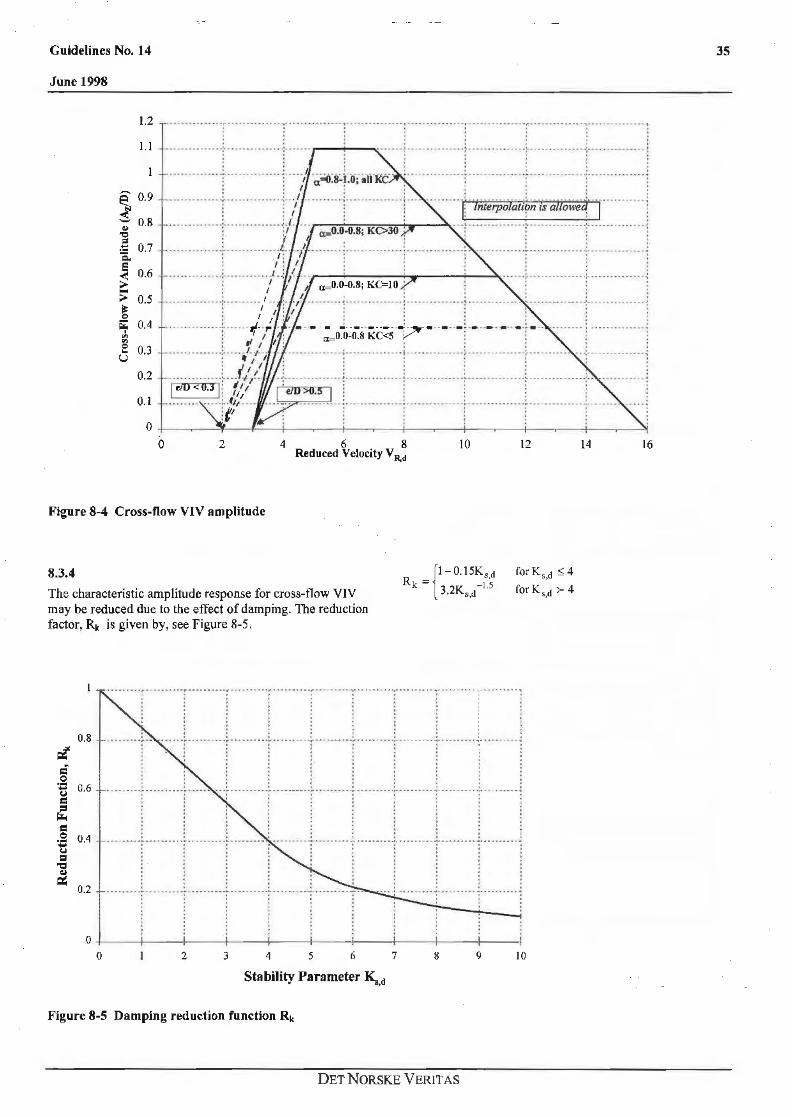
Guidelines No. 14
June 1998
1.2
l.I
,...... 0.9 e
~ 0.8 '-'
G>
"' = 0.7 .<:::: -a.
~ 0.6 -;;... 0.5 ~ ~ 0.4 J,
"' ~ 0.3 ... u
0.2
0. 1
2 4 6 8 Reduced Velocity VR.d
IO 12
Figure 8-4 Cross-flow VIV amplitude
8.3.4
The characteristic amplitude response for cross-flow VIV may be reduced due to the effect of damping. The reduction factor, Rk is given by, see Figure 8-5.
forKs,d ~ 4
for Ks,d >- 4
~
= 0 :e 0.6
~ c:
.Si 0.4 -c.i ::I
~ 0.2
0
· · · ·· · · · ., ....... ···: ·· · · · · · · · ·r · ·· · ·· · · ··: · ·· · · ·· · ·; ·--·-· ·· · ·r ·· · · · ··· · ····· · ···· .... :. · ·· · · ·-· · ··· ····· ·· · · ~ . . . . . . . . . . ·- ·· ·r· ·· .... -· ·-·r · · · -· ···· ·r ·· · ·· -----r-------·-·r· -· -· · ··· -~-· · · -· ----~------···· ~- ......... .: : : j •
. . I o t o
' > o o o o o I I o .... ...................... --·· ......................................................... ................................ ............... .... . . . . . . . . ' I t o o o ' 0 I 0 0 I . . . '
. . --- . ---- ·: ...... ·-. ·~-·. -··. -- -~--. - ·-· -- -:- -- · --· ---:- -·-····. --: . ··--·----:---- --- ·- --:-. ...... -.... ~
: : : l : : i : ~
. . . _________ ..... .......... ...... -----------······ .. ····-- ·-.. ··-·------ - .... ..... ........ . • I o o • o 0 • . . . . . . . . . . . . . . . . . . . . . . . . . . . . . . .
2 3 4 5 6 7 8 9 10
Stability Parameter ~,d
Figure 8-5 Damping reduction function Rk
DETNORSKE VERITAS
35
14 16
36
8.3.5
The normalised amplitude curves in Figure 8-4 to a large degree embody all available test result. However, the following comments apply:
• The response for (e/D < 0.5) is (in reality) not governed by vortex shedding and should in a narrow sense not be characterised by VIV parameters as VR and KC. Tue indicated response curve is considered conservative in general.
• The response for low KC values is associated with a large uncertainty and the number of test data is scarce. For KC< 5 the response is not governed by VIV but rather linked to wave induced water particle motions, and one sided vortex shedding. Typical maximum response at V R between 2.5 and 3 .0 occur at fo/fw.,. 2.
• In case f0 < 3fw the criticality should be assessed, e.g. from dedicated tests or applying a force model.
9. Force Models
9.1 General
9.1.1
In principle, force models may be used for both vortex induced and direct wave and current dominated loads if appropriate formulations of force models exist and reliable and consistent data are available for calibration.
9.1.2
The well-known Morison's equation is presented herein while functional requirements are provided for general force models for combined flow conditions.
Several analytical force models for cross-flow have been proposed and calibrated using experimental data, see e.g. Sumer & Freds0e, (1997) and Blevins, (1994) for a detailed introduction. However, generally applicable force models do not exist and an empirical response model reflecting observed pipeline response in a variety of flow conditions is at present superior.
9.1.3
The stress range to be applied in section 7.2 may be calculated explicitly introducing the force model as a loading term in the equation of motion for the free span scenario. The solution may apply time domain solutions or frequency domain solution using linearization techniques.
The set of safety factors given in section 7.4 is linked to a consistent definition of characteristic parameters and models. They have not been calibrated to the force model, and, if
Guidelines No. 14
June 1998
applied, the adequacy must be evaluated on a case to case basis.
9.2 In-line direction
9.2.1
The in-line force per unit length of a pipe free span is determined using the Morison's equation:
where:
p water density
D outer pipe diameter (including any coating)
U instantaneous (time dependent) flow velocity
y in-line displacement of the pipe
drag coeffici~nt.
ine11ia coefficient
(Ca+ l) where c. is the added mass coefficient
differentiation with respect to time.
9.2.2
In general, the drag and inertia coefficient is given by:
Co= Cn(Rc,KC,o.,(c/D),(k/D),(Az ID))
CM= CM(Rc,KC,a,(e/D), (klf)))
where Re is the Reynolds number, KC is the Keulegan· Carpenter number, a is the current velocity ratio, (e/D) is the gap ratio, (k/D) is the pipe roughness and (Az/D) is the crossflow vibration amplitude. Definitions are given in section 5.
9.2.3
In Figure 9-1 and Figure 9-2 drag and inertia coefficients are given as function of KC and ex., i.e. CL>(KC,a.) and CM(KC,cx.). Corrections due to the influence of the seabed may be taken from Figure 5-1. Fuither, the effect of the pipe roughness and increase oft11e drag coefficient due to cross-flow vibration may be taken from Classification Note No. 30.5.
DET NORSKE VERITAS

Guidelines No. 14
June 1998
2.0 ..,....----...· .................... ;·····--· .. ···-- ·· ·--1·--... ............. .
Q
u
1.8
l.6
1.4
c 1.2 ~ ·o e 1.0 ~ Q
u Oil 0.8 <I'S N
~ 0.6 .
0.4
0.2
: I i . . ...................... , ..... ········-·······1·············· ....... .
: :
····-···············r····················!····-··············· . . ····················t···················-.:····················
f ; ... ··············f····················i···················· . . .... a .......... ..
0.0
. . . . . . . ...................... . ...... ............. ................. .............................................. ... . ...... .................. ............. ..... .... . ........ . : ! i : i <0.5
gap ratio .e > . . . ·· roughness (k/D)=l/200 .. i ..................... f ................... T" ................. T ................ .
t t I o . . . . t t I I
o o 0 0 I ... ..................... ................................ --·····--~--·········.-······ -· ······· .......... --·- ···-···----.................................. .. . . . . . . . . . . . . o.o ..._ ____ _,_· ___________ _,_ ____ _,_· __________ ~
0 10 20 30
KC 40 50 60
Figure 9-1 Drag coefficient C0 versus KC and«
2.0 i-----=··--··~···--····--····------~---------·--·--------:--···---- · ·-- · ·----··;·-- · ·------······--··:··· · · ·· · ·· · · -- · ·--···, . . . . . . . . . ; .. ------· ---·---·---- ~-- · -- · · -- ---- ---- · ---r --- ----- --- ---- ---- --~----~- -- ------- ---1 . . . ~o .
1.8
;:oo,.........,..._ ....... ____ ~---.-;: .. !:P .... ........ 1 ~ 0.2
1.4 ................ .. ................ . . . . ' . .................................... ............... .... P-••·--··""······ ·--··--·· --· --· -- ....... .. > • •
: : 0.3 : ' . . . .
~ 1.2 .............. ---·~· ·· .... . ...... . .. ~ ............ ....... ~ .. . .................. :... ................... ; .................. j ·u : : · o 4 e : ---~~~: ~~~~~~~~____..: . ~ t.o -1----~-- .... ~ ................ - ~ - .. -· ......... ---:--· ...................................... T .............. ----j u 'f 0.8
. . • • I j • ~ ..................... ~ ..................... f .................... T.<o:s--· ........ j
~
= ' o I ' '
... 0.6 . ' ' . ' o • I I o ---· ..................................................... ~ ................ - .................................. _ ............................................. -·····-······· .............. . . . . ' . .
gap ratio e > . : : ! : : : : i I :
0.4 .... roughness (k/D)=l/200 "j" ................... ( ................... f ................... T ................... j ; ; : ! : o.2 .................... T .................... r··················--1··--··--··---........ f .................... 1··--················~ + ' o o I . . . . . . . . ' .
0.0 -1------+'-----+------1------i-------'1------~· 0 10 20 30
KC
40
Figure 9-2 Inertia coefficient CM versus KC and a,
DETNORSKE VERITAS
50 60
37
38
9.2.4
Both time domain and frequency domain solutions are allowed. A time domain solution may account for all significant non-linearities but is in general very time consuming if a large number of sea-states are to be analysed. For fatigue analysis a frequency domain solution (if thoroughly verified) is more tractable since it facilitate analyses of a very large number of sea-states at a small fraction of the time required for a time domain solution, see M0rk and Fyrileiv (1998).
9.3 Cross-flow direction
9.3.t
Models describing the vortex shedding cross-flow forces are semi-analytical and include coefficients that are derived from test data. Generally, the models are limited in tenns of their physical basis and the range of application. A number of models can treat steady current conditions, see e.g. Blevins, (1994). Others have been developed for harmonic flow (regular waves) conditions see e.g. Bearman, (1984) and Verley ( 1982). Models, which treat general flow conditions, are more complex and the wide parameter range and conditions to be covered makes it necessary to include a number of different terms each justified by different physical conditions or parameters.
10. References Bearman, P. W., Graham, J.M. R, Obasaju, E. D., "A Model Equation for the Transverse Forces on Cylinders in Oscillatory Flows", Applied Ocean Research, Vol. 6, No. 3, pp. 166-172, 1984.
Blevins, R.D., "Flow-Induced Vibrations", Krieger Publishing Company, Florida, 1994
Bruschi, R. & Vitali, L., "Large-Amplitude Oscillations of Geometrically Non-linear Elastic Beams Subjected to Hydrodynamic Excitation", JOMAE, Vol. 113, May, 1991.
BSI PD6493, "Guidance on Methods for Assessing the Acceptability of Flaws in Fusion Welded Structures", British Standard Code of Practice, 1991
DNV, "Rules for Submarine Pipeline Systems", 1981
DNV, "Rules for Submarine Pipeline Systems", 1996
DNV Classification Note No. 30.2, "Fatigue Strength Analysis for Mobile Offshore Units", 1984.
DNV Classification Note No. 30.5, "Environmental Conditions and Environmental Loads", 1991.
DNV RP E305, "On-bottom Stability Design of Submarine Pipelines", 1988.
Fyrileiv, 0., M0rk, K.J., Kathrud, K., & Sortland, L "Free Span Assessment of the Zeepipe IIA Pipeline", OMAE'98, Lisboa, July 6-9, 1998.
Guidelines No. 14
June 1998
Fyrileiv, 0. & M0rk, K.J., "Assessment of Free Spanning Pipelines using the DNV Guideline", JSOPE'98, Montreal, Canada, May 24-29, 1998.
MULTISPAN Project, "Design Guideline. VIV of Free Spanning Pipelines. Part I: Steady Current Loading'', DNV report 95-3 134, H0vik, Norway, 1996.
M0rk, K.J. , Vitali, L. & Verley, R., "The l'vfULTISPAN Project: Design Guideline for Free Spanning Pipelines", Proc. of OMAE'97 conf., Yokohama, Japan, April 13-17, 1997.
Mmk, K.J. & Fyrileiv, 0. "Fatigue Design According to the DNV Guideline for Free Spanning Pipelines", OPT'98, Oslo, Norway, February 23-24, 1998.
M0rk K.J. , Fyrileiv, 0., Verley, R., Bryndum, M. & Bruschi, R. "lntroduction to the DNV Guideline for Free Spanning Pipelines", OMAE'98, Lisboa, July 6-9, 1998.
NORSOK Standard "Design Principles. Steel Structures. Armex C: Fatigue Strength Analyses", 1998
Sumer B.M. & Freds0e, J. "Hydrodynamics around Cylindrical Structures", Advanced Series on Ocean Engineering - Volume 12, World Scientific, London, 1997.
Tura, F., Dwnitrescu, A., Bryndum, M. B. & Smeed, P.F. "Guidelines for Free Spanning Pipelines: The GUDESP Project", OMAE'94, Volume V, pp 247-256, Houston, 1994.
Verley, R., "A Simple Method of Vortex-Induced Forces in Waves and Oscillating Currents'', Applied Ocean Research, Volume 4, No. 2, 1982.
DETNORSKE VERITAS