freight data from intelligent transportation system devices · pdf filefreight data from...
TRANSCRIPT

Research Report
Research Project T1803, Task 25 Intermodal Data
FREIGHT DATA FROM INTELLIGENT TRANSPORTATION SYSTEM DEVICES
by
Mark E. Hallenbeck Edward McCormack Director Senior Research Engineer
Jennifer Nee Duane Wright Research Engineer Systems Analyst Programmer
Washington State Transportation Center (TRAC) University of Washington, Box 354802
University District Building 1107 NE 45th Street, Suite 535
Seattle, Washington 98105-4631
Washington State Department of Transportation Technical Monitor
Bill Legg Assistant ITS Program Manager Advanced Technology Branch
Prepared for
Washington State Transportation Commission Department of Transportation
and in cooperation with U.S. Department of Transportation
Federal Highway Administration
July 2003


TECHNICAL REPORT STANDARD TITLE PAGE 1. REPORT NO. 2. GOVERNMENT ACCESSION NO. 3. RECIPIENT'S CATALOG NO.
WA-RD 566.1 4. TITLE AND SUBTITLE 5. REPORT DATE
FREIGHT DATA FROM INTELLIGENT TRANSPORTATION July 2003 SYSTEM DEVICES 6. PERFORMING ORGANIZATION CODE 7. AUTHOR(S) 8. PERFORMING ORGANIZATION REPORT NO.
Mark E. Hallenbeck, Edward McCormack, Jennifer Nee, Duane Wright 9. PERFORMING ORGANIZATION NAME AND ADDRESS 10. WORK UNIT NO.
Washington State Transportation Center (TRAC) University of Washington, Box 354802 11. CONTRACT OR GRANT NO.
University District Building; 1107 NE 45th Street, Suite 535 Seattle, Washington 98105-4631
Agreement T1803, Task 25 12. SPONSORING AGENCY NAME AND ADDRESS 13. TYPE OF REPORT AND PERIOD COVERED
Research Office Washington State Department of Transportation Transportation Building, MS 47370
Research Report
Olympia, Washington 98504-7370 14. SPONSORING AGENCY CODE
Tom Hanson, Project Manager, 360-705-7975 15. SUPPLEMENTARY NOTES
This study was conducted in cooperation with the U.S. Department of Transportation, Federal Highway Administration. 16. ABSTRACT
As congestion increases, transportation agencies are seeking regional travel time data to determine exactly when, how, and where congestion affects freight mobility. Concurrently, a number of regional intelligent transportation systems (ITS) are incorporating various technologies to improve transportation system efficiency. This research explored the ability of these ITS devices to be used as tools for developing useful historical, and perhaps real-time, traffic flow information.
Regional transponder systems have required the installation of a series of readers at weigh stations in ports, along freeways, and at the Washington/British Columbia border. By linking data from these readers, it was possible to anonymously track individual, transponder-equipped trucks and to develop corridor-level travel time information. However, the research found that it is important to have an adequate number of data points between readers to identify non-congestion related stops. Another portion of this research tested five GPS devices in trucks. The research found that the GPS data transmitted by cellular technology from these vehicles can provide much of the facility performance information desired by roadway agencies. However, obtaining sufficient amounts of these data in a cost effective manner will be difficult. A third source of ITS data that was explored was WSDOT’s extensive loop-based freeway surveillance and control system.
The output from of each of the ITS devices analyzed in this research presented differing pictures (versions) of freight flow performance for the same stretch of roadway. In addition, ITS data often covered different (and non-contiguous) roadway segments and systems or geographic areas. The result of this wide amount of variety was an integration task that was far more complex then initially expected.
Overall, the study found that the integration of data from the entire range of ITS devices potentially offers both a more complete and more accurate overall description of freight and truck flows. 17. KEY WORDS 18. DISTRIBUTION STATEMENT
Freight data, ITS devices, data collection, data management
No restrictions. This document is available to the public through the National Technical Information Service, Springfield, VA 22616
19. SECURITY CLASSIF. (of this report) 20. SECURITY CLASSIF. (of this page) 21. NO. OF PAGES 22. PRICE
None None

DISCLAIMER
The contents of this report reflect the views of the authors, who are responsible
for the facts and the accuracy of the data presented herein. The contents do not
necessarily reflect the official views or policies of the Washington State Transportation
Commission, Department of Transportation, or the Federal Highway Administration.
This report does not constitute a standard, specification, or regulation.


Table of Contents
Section Page
iii
Executive Summary......................................................................................................... ix
1. Introduction.................................................................................................................. 1
ITS FReight Data Benefits............................................................................................ 2 Project Approach .......................................................................................................... 3
Inventory Freight-Oriented ITS Systems................................................................ 4 Acquire Data ........................................................................................................... 4 Clean and Locate Data ............................................................................................ 4 Develop Usable Performance/Usage Data.............................................................. 4 Develop Recommendations .................................................................................... 5
2. Wireless GPS Devices .................................................................................................. 6
GPS Analysis Steps....................................................................................................... 8 Conversion of GPS Data to Usable GIS Formats ................................................... 8 Analytical Output Using the GPS Data ................................................................ 14
Geographic Distribution of the GPS Data Collected .................................................. 22 Instantaneous Speed versus Segment Travel Time Speed.......................................... 24
Comparison Between GPS and Freeway Surveillance System Speeds ................ 26 Comparison of GPS and Freeway Survellance System Travel Times.................. 30
Analysis of Device Reporting Frequency ................................................................... 36 Conclusions about the Use of GPS Data..................................................................... 39
3. Truck Transponders.................................................................................................. 42
Transponder Analysis Steps........................................................................................ 45 Identifying Available Travel Times...................................................................... 47 Identifying Best Available Travel Time ............................................................... 48 Removing Outliers ................................................................................................ 49
Testing Output ............................................................................................................ 51 WIM Transponders ............................................................................................... 51 Border Transponders............................................................................................. 53
Data Limitations.......................................................................................................... 55 Spatial Data Coverage........................................................................................... 56 Temporal Data Coverage ...................................................................................... 57
Conclusions About the Use of Transponder Data....................................................... 63
4. FLOW System Data................................................................................................... 65
FLOW Data Analysis.................................................................................................. 68 Conclusions................................................................................................................. 74

Table of Contents (Continued)
Section Page
iv
5. Integration of Data Sets............................................................................................. 75
Data Acquisition ......................................................................................................... 75 Financial and Organizational Cost........................................................................ 76 Privacy .................................................................................................................. 78
Data Manipulation and Quality Assurance ................................................................. 79 A Design for Integrating ITS Data.............................................................................. 81 Output reports ............................................................................................................. 83 Additional Data Sources ............................................................................................. 84
6. Summary...................................................................................................................... 86
Truck Transponders .................................................................................................... 86 Wireless GPS .............................................................................................................. 87 Freeway Surveillance and Control System................................................................. 88 Data Integration .......................................................................................................... 88
References........................................................................................................................ 91
Appendix A. Assigning Mileposts to GPS Data ........................................................ A-1

List of Figures
Figure Page
v
1. GPS device in Truck ......................................................................................... 7 2. Map Matching Problem .................................................................................... 11 3. Example of a Congestion Contour Graphic from Freeway Data...................... 16 4. Congestion Contour Graphic for Southbound I-405 from GPS Data ............... 16 5. Congestion Contour Graphic for Northbound I-405 from GPS Data ............... 17 6. The Distribution of Speeds Reported by the GPS Devices Northbound
on I-405 through Renton................................................................................ 18 7. GPS Reported Speeds versus Location of Truck.............................................. 20 8. Reported GPS Speed versus Time of Day ........................................................ 20 9. Comparison of Alternative Speed Estimates from GPS Devices ..................... 31 10. Comparison of Instantaneous Speeds with Computed Average Segment
Speeds on an Arterial ..................................................................................... 33 11. Arterial Speeds versus Location ....................................................................... 34 12. Distribution of Speeds on State Route 99 ......................................................... 35 13. Map of AVI reader locations ............................................................................ 43 14. Typical Truck Windshield Transponder ............................................................ 43 15. Usable Truck Tags for Estimating Travel Time ............................................... 46 16. Data Filtering Process ....................................................................................... 51 17. Average Truck Speed (5-Minute Interval) - Unfiltered..................................... 52 18. Average Truck Speed (5-Minute Interval) - Filtered........................................ 52 19. Average Truck Speed (Rolling Hour)............................................................... 53 20. Duration near the Border – Unfiltered data ...................................................... 54 21. Duration near the Border – Filtered Data ......................................................... 55 22. Frequency of Truck Tag Reads......................................................................... 57 23. Gap between Trucks, Ridgefield to Fort Lewis ................................................ 58 24. Gap between Trucks, Fort Lewis to Stanwood Bryant ..................................... 58 25. Gap between Trucks, Ridgefield to Stanwood Bryant...................................... 59 26. Port of Tacoma to Border: Sample Travel Time .............................................. 61 27. Port of Tacoma to Border: Sample Speed......................................................... 61 28. Port of Seattle to Border: Sample Travel Time ................................................ 62 29. Port of Seattle to Border: Sample Speed........................................................... 62 30. Freeway Surveillance System Coverage........................................................... 66 31. Average Operating Condition of I-5 By Time of Day and Location................ 69 32. Frequency of LOS F Congestion on I-5............................................................ 70 33. Location Specific Volume, Average Speed, and Frequency of Congestion.71 34. Use of Location Specific Graphics To Examine Performance Trends ............. 71 35. Travel Time Performance and Congestion Frequency For a Corridor ............. 73 36. 90th Percentile HOV Lane Speed, and Frequency of Performance Standard
Failure ............................................................................................................ 73 37. Schematic of Proposed Integrated Data Archive .............................................. 82

List of Figures (Continued)
Figure Page
vi
A-1. Selected GPS points (right side) that are clearly not on a route ....................... A-3 A-2. The logic for determining increasing or decreasing direction .......................... A-5 A-3. The Field Calculator utility, in ArcMAP 8.1, with the VBS Script
algorithm loaded. ........................................................................................... A-5 A-4. This section of State Route 167 increases in a southeastern direction ............. A-6 A-5. The “Select By Attribute” Window.................................................................. A-7 A-6. “Decreasing” GPS points have been “snapped” to the closest location on a
decreasing route. ............................................................................................ A-9 A-7. GPS point for a vehicle traveling in an increasing direction on I-405 has
been erroneously snapped to SR-181............................................................. A-10

List of Tables
Table Page
vii
1. Data Distribution........................................................................................................... 23 2. Comparison of GPS Derived Performance Data and Freeway
Surveillance Data on a “Poor Day” ........................................................................... 28 3. Matching Truck Tags.................................................................................................... 48 4. Frequency of Data Points.............................................................................................. 59 5. ITS Device Summary.................................................................................................... 89


ix
EXECUTIVE SUMMARY
A major impact on freight movement is roadway congestion. As congestion
increases, transportation agencies are seeking regional travel time data to determine
exactly when, how, and where congestion affects freight mobility. Concurrently, a
number of regional Intelligent Transportation Systems (ITS) are incorporating
transponders, roadway loops, global positioning systems (GPS), and other devices to
improve transportation system efficiency. Potentially, the accumulation of location and
speed information from these devices could produce enough information about truck
movements on roads to develop meaningful travel data to help answer those questions.
The freight information developed from ITS devices can be used as the
foundation for planning studies. Freight-oriented travel data are needed to identify truck
bottlenecks, to explore the reliability of freight movements, and to determine the
frequency and costs of nonrecurring events such accidents and weather. Such
information could justify the development of freight-oriented highway construction and
ITS projects. This information could also assist in identifying and modifying the impacts
of activities such as port gate closures and sporting events.
This research project explored the ability of ITS devices to be used as tools for
developing useful historical, and perhaps real-time, traffic flow information specifically
related to truck movements. The Puget Sound region’s diverse ITS present an
opportunity for exploring the collection, analysis, and overall usability of truck flow data
derived from ITS devices.
The first portion of this research tested data from five fleet management GPS
devices in trucks. The research found that the GPS data transmitted by cellular

x
technology from these vehicles can provide much of the facility performance information
desired by roadway agencies. However, obtaining sufficient amounts of these data in a
cost effective manner will be difficult. The biggest challenge is the cost of collecting the
data, although considerable effort is needed to manage and analyze the data once they
have been obtained from the field.
For analyzing specific roadway projects that are of interest to commercial freight
carriers, it might not be difficult to obtain volunteer GPS probes, even without the
incentive to the carriers of gaining real-time location access information. However,
considerable care must be given to the selection of the GPS probe truck fleet if “holes”
are to be avoided in the time-of-day, day-of-week, and geographic coverage of the
performance monitoring system.
Another ITS in the Puget Sound region that could be used to collect freight data is
Washington’s Commercial Vehicle Information Systems Network (CVISN), which
employs windshield-mounted truck transponders to collect information at freeway
speeds. A related but separate system is the Washington State Department of
Transportation’s (WSDOT) and U.S. Custom’s in-bond container system, which uses the
same transponders for container tracking and as a border pre-arrival system.
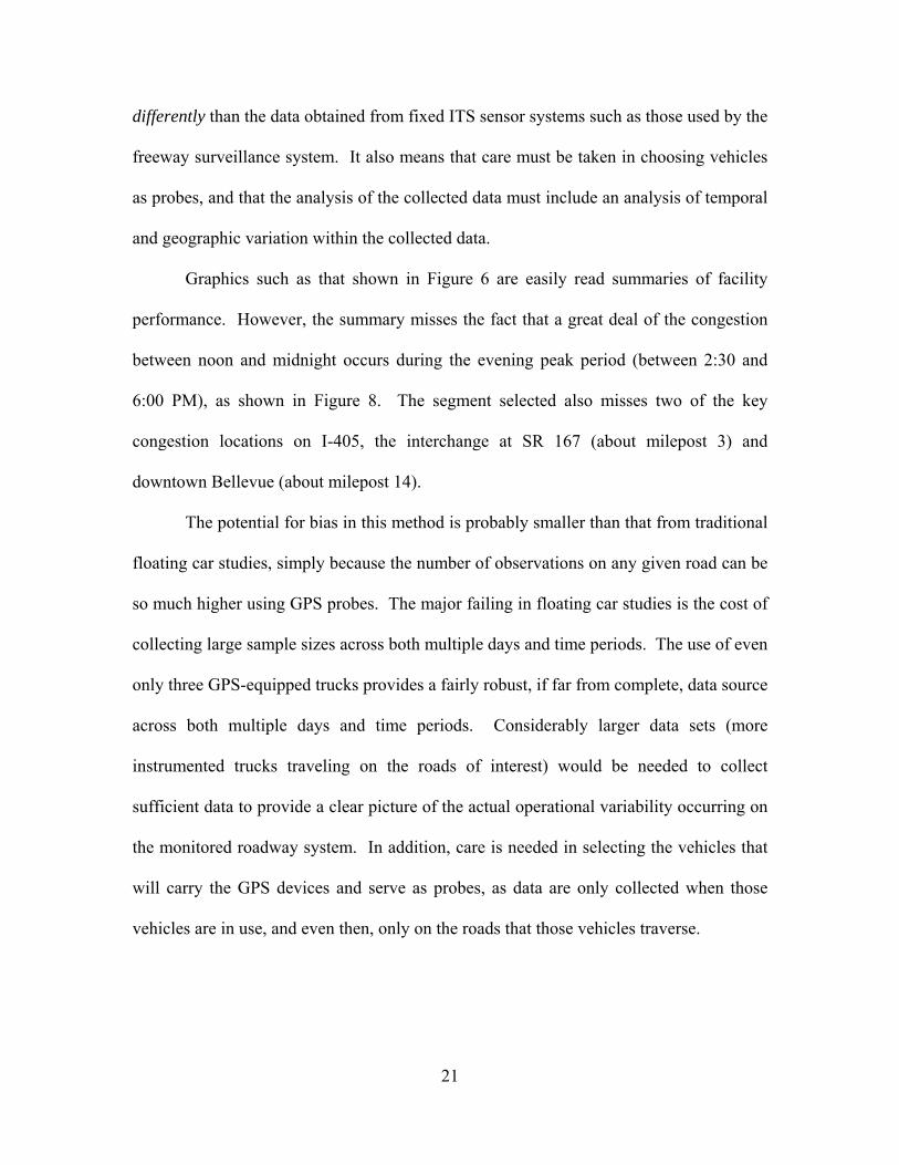
These transponder systems have required the installation of a series of readers at
weigh stations, in ports, along freeways, and at the Washington/British Columbia border.
By linking data from these readers, it was possible to anonymously track individual,
transponder-equipped trucks and to develop corridor-level travel time information.
However, when using truck transponder data, this research found that it is important to
have an adequate number of data points between readers to identify non-congestion

xi
related stops. Frequent data points are required to filter out trips that contain extra time
when a truck stops between readers. The truck transponder data collected at the
international border had potential for estimating border delay to understand border travel
conditions such as queuing patterns.
A third source of ITS data that was explored was WSDOT’s extensive roadway
loop-based freeway surveillance and control system (FLOW). The use of FLOW data for
performance analysis is extremely powerful but with significant limitations. The biggest
limitations are that the data are available only for a limited set of roadways, and the cost
of surveillance system expansion means that additional data collection can only occur as
part of the expansion of the WSDOT’s surveillance and control system. Another, and
somewhat less important, limitation is that the large size of the data archive creates some
significant data handling and quality control problems.
The output from each of the ITS devices analyzed in this research presented
differing pictures (versions) of freight flow performance for the same stretch of roadway.
In addition, ITS data often covered different (and non-contiguous) roadway segments and
systems or geographic areas. The result of this wide amount of variety was an integration
task that was far more complex than initially expected.
Integration of data from ITS devices initially requires acquiring the data. This can
be a problem because there are costs associated with data archiving, and because the
storage and use of some ITS data raise privacy concerns. Once the data are acquired they
need to be checked for validity and placed into common data formats. One of the key
tasks in the quality assurance effort is to correctly assign data to the roadway network.
This task typically uses GIS software but depends on an accurate digital base map.

xii
Another acquisition concern is to ensure that different ITS devices have accurate time
stamps so they can be integrated.
In many cases the research found that two ITS data collection systems could
develop “similar but different” data items. It is very important that these differences be
clearly identified as part of any integration effort because these “different” data items can
lead to questions about the accuracy of the data being collected.
The data from the various ITS device need to be stored, which typically requires a
computer system that meets the basic storage, access, and reporting requirements of the
archive. This project investigated a GIS-based technology that is designed to integrate
independent archives to allow “operators” of archives to build and operate each archive
in the manner in which it is the least costly and most useful to them. This format allows
unlimited expansion to other ITS and data systems. The information then can be placed
in an output report, which can present a range of useful travel and flow statistics.
Overall, the study found that the integration of data from the entire range of ITS
devices potentially offers both a more complete and more accurate overall description of
freight and truck flows.

1
1. INTRODUCTION
A major impact on freight movement is roadway congestion. As congestion
increases, organizations such as the Puget Sound Regional Council (PSRC) and the
Washington State Department of Transportation (WSDOT) are seeking regional travel
time data to determine exactly when, how, and where congestion affects freight (and
personal) mobility. Concurrently, a number of regional Intelligent Transportation
Systems (ITS) are incorporating transponders, roadway loops, global positioning systems
(GPS), and other devices to improve transportation system efficiency. Potentially, the
accumulation of location and speed information from these devices could produce
enough information about freight movements to develop meaningful travel data to answer
those questions.
This research project, funded as part of a Federal Highway Administration effort
to improve freight and goods movement, explored the ability of these ITS devices to be
used as tools for developing useful historical, and perhaps real-time, traffic flow
information. The region’s diverse ITS present an opportunity for exploring the
collection, analysis, and overall usability of ITS flow data.
As one part of this research, five GPS devices designed to be used as a truck fleet
management system were tested as data collection devices. The GPS devices were
mounted in truck cabs and a cellular connection was used to report the trucks’ positions
and other information. Such devices could potentially offer information about travel
times and freeway speeds.
Another ITS that could be used to collect freight data include Washington’s
Commercial Vehicle Information Systems Network (CVISN) system, which employs

2
more than 20,000 windshield-mounted truck transponders to collect information at
freeway speeds. A related but separate system is WSDOT’s and U.S. Custom’s in-bond
container system, which uses the same transponders for container tracking and a
U.S./Canadian border pre-arrival system. As part of both these transponder systems,
public and private agencies have placed readers at weigh stations, in ports, along
freeways, and at the Washington/British Columbia border. By using software to link
these readers, it would be possible to anonymously track individual, tag-equipped trucks
and thus determine regional and corridor travel times and patterns.
In the greater Puget Sound region, WSDOT has an extensive loop-based freeway
management system known as the freeway surveillance and control system (FLOW).
This system includes 300 loop locations that offer information about freeway volume and
speeds and, in limited cases, truck volume data.
This research effort explored the strengths and limitations of the data from these
devices. As part of this process, the manipulation, clean up, and analysis of the data were
examined. Conclusions and recommendations for an overall data program were
developed.
ITS FREIGHT DATA BENEFITS
The freight information developed from ITS devices could be used as the
foundation for local and regional planning. Freight-oriented travel data are needed to
identify freight movement bottlenecks, to explore the reliability of freight movements,
and to determine the frequency and costs of nonrecurring events such accidents and
weather. Such information could justify the development of freight-oriented highway

3
construction and ITS projects. This information could also assist in identifying and
modifying the impacts of activities such as port gate closures and sporting events.
Better freight data would certainly benefit a range of transportation agencies. On
a basic level, these ITS-derived data could provide a convenient picture of urban freight
movements. At a project level, these data could help transportation agency staff correlate
existing and predicted roadway conditions with changes in freight movements. Such a
process would mean that roadway construction projects could more effectively address
concerns about regional freight mobility. On a regional level, these data could help
transportation agency staff address many questions centered on freight mobility and
economic growth. Using indicators developed from such data, agency staff would be
better able to discuss the impacts of increased regional congestion on truck flows and
freight mobility. This, in turn, could help answer basic policy questions.
Specific application of these data could include the following:
• guidance on where to locate freight-oriented variable message signs
• routing information for motor carrier dispatchers
• determine the freight impact roadway construction
• information on the effects of changes in terminal operations
• calibration information for freight modeling
PROJECT APPROACH
The research approach followed these general steps:

4
Inventory Freight-Oriented ITS Systems
The project’s first step examined the Puget Sound region’s ITS systems and
determined whether they had the capability to collect data pertaining to truck flows and
other freight movements. Data from the following ITS devices were used:
• truck fleet management wireless GPS
• CVISN weigh-in-motion transponders
• in-bond border container clearance and tracking transponders
• WSDOT’s freeway control and surveillance system (FLOW)
Acquire Data
Next the project explored methods to acquire and link data from each of the ITS
identified in the previous step. The focus was on obtaining and consolidating existing
data, as well as on database management.
Clean and Locate Data
For each of the ITS devices, this step was concerned with how to develop a
common data format and how to determine what data needed to be discarded. Also
addressed were questions such as how to assign (i.e., geolocate) transponder and GPS
data to the roadway network. This was necessary to determine whether the target vehicle
was on an arterial or a freeway. This required accurate GIS and roadway locations.
Develop Usable Performance/Usage Data
This step focused on how to develop performance and usage information from the
ITS devices data. The task emphasized the development of report outputs that would be
usable for improving policy and operational decisions by both public agencies and private
firms.

5
The ITS data were explored as a source of information for the following
categories:
• vehicle classifications and volumes on the roadway segments
• the reliability of freight flows (i.e., if congestion significantly interfered with delivery schedules)
• the time and location of recurring congestion.
Develop Recommendations
Finally, the project developed recommendations about the usability of ITS
devices as a way to explore and manage freight flow on the roadway system. The value
of data integrated from a range of ITS devices was discussed.

6
2. WIRELESS GPS DEVICES
This portion of the research explored the use of data obtained from wireless
global positioning systems (GPS) devices installed in trucks. The devices were
developed by AirTrak for commercial vehicular fleet management and combined GPS
technology with a cellular reporting feature. The devices were designed to allow
commercial vehicle operators to monitor the location of a truck or other assets and
communicate back to those assets. This research used five borrowed devices for about a
year. They were installed in five trucks that operated mainly in the Puget Sound region,
two based out of Seattle (Puget Sound Truck Lines) and three based out of Tacoma (two
with CSX drayage and one with Puget Sound Truck Lines). The installation process
included putting the GPS device and antenna in the trucks (Figure 1) and placing the
tracking software at the Washington State Transportation Center (TRAC) and at Puget
Sound Freight Lines. The drivers of several of the trucks also received a short training
session on how to turn the device on and off. TRAC paid the wireless charges.
Each time the GPS device reported, vehicle-specific speed, time, travel direction
(bearing), and location were collected. This, in turn, provided point estimates of roadway
speed, as well as the ability to compute roadway travel time. It also allowed the research
team to explore “roadway performance” on the basis of periodic reports of instantaneous
vehicle speed, versus direct measurement of vehicle trips along specific roadway
segments.

7
Figure 1. GPS device in Truck
Use of the devices for a year resulted in 98,000 location reports. The devices
were operated with various airtime plan configurations (meaning location reports were
obtained every 30 seconds, 60 seconds, whenever the vehicle made a 45-degree heading
change, and a combination of time intervals and heading changes). This was done to
relate the cost of the plan to the usefulness of the resulting data. The costs for the
wireless charges for 4,500 positions a month were $60.00 per vehicle. Each additional
500 positions cost $7.00 a month per vehicle.

8
The different communication plans were tested to determine the extent to which
communications could be minimized without losing the positional information needed to
track vehicle movements through dense roadway networks.
GPS ANALYSIS STEPS
Conversion of GPS Data to Usable GIS Formats
To make the GPS data useful, they had to be tied to the earth’s surface with a
geographic information system (GIS). A recent NCHRP report (Czerniak 2002)
discussed the integration of GPS data into a GIS and highlighted some of the problems
found while locating GPS data as part of this effort.
Several sources of GPS error can complicate the collection of GPS location data.
The NCHRP report lists errors caused by
• GPS satellite limitations
• atmospheric distortion
• GPS device limitations.
The GPS devices used in this project created errors in several ways. For example,
errors that could be attributed to satellite limitations and atmospheric distortions showed
up as truck movement (jitter), even when the truck had a speed of zero. This jitter also
complicated matching the reads to an underlying digital street map.
Other GPS device limitations included signal loss as trucks passed under
overpasses and into areas with tall buildings. Missing reads and/or lack of GPS location
reports tended to be less of a problem for this project than jitter. Other areas in the nation
with many tall buildings or natural terrain conditions that limit GPS satellite observation
or device communications might experience more problems with GPS signal loss. Signal

9
loss was rarely a problem in this project because the test vehicles most often traveled on
freeways and other roadways with good GPS signal reception.
Another issue that complicated locating the GPS reads stemmed from the fact that
the underlying digital street map often did not match the GPS points. The problem is
usually caused by use of a map that was created with GPS reads before the removal of the
“selective availability” feature. This “feature,” intentionally introduced by the U.S.
Defense Department, caused a lack of accuracy in GPS readings and resulted in the
distortion of maps based on early GPS readings.
A unique aspect of this analysis, which made both GPS distortion and map
matching errors more difficult to deal with in comparison to more conventional uses of
GPS for roadway performance monitoring, was that the trips being taken by the tracked
trucks were not known by the analysis team before they were taken. Most GPS data
collected for travel time monitoring are collected as part of specific data collection runs.
During these runs, the staff knows what route is being taken, in what direction the vehicle
is traveling, and when the data collection run begins and ends. In this field test, none of
these factors was true. The project team did not know what route a truck was taking,
when it was stopping, and in which direction it was proceeding at any given time.
The advantages of the tested technique were that data were collected on routes
actually used by the trucking fleet, and the agency that collected data did not need to pay
the driver of the vehicle or pay for the cost of operating that vehicle. The fact that the
data came from roads “normally” used by trucks meant that the data would likely serve as
a good measure of the performance of the roads that were important to the fleet being
monitored. In addition, as the fraction of trucks being monitored grew relative to the

10
number of trucks operating in the region, these data would also serve as an excellent
measure of the relative importance of different roads to trucks. (That is, the road
segments with the greatest number of observations would be those used the most and
would, therefore, also be the most important for freight mobility.) This would be doubly
beneficial because modern traffic data collection equipment has a very hard time
accurately monitoring truck volumes in urban traffic conditions. Taken together, these
two factors would serve as an incentive for fleets to allow their trucks to be tracked. (“If
you participate and your trucks are stuck in congestion, we’ll know about it, and those
problem spots will receive higher rankings in the prioritization process for projects that
relieve congestion.”)
However, the lack of knowledge about the location and direction of any given
truck at any given time caused the analysis of GPS data to be considerably more difficult
than it would have been if the test vehicles had been traveling known routes. For
example, the fact that a vehicle location did not match to a roadway segment could not be
immediately traced to poor correlation between GPS and GIS location referencing
systems. The reason for this was that during our test, when a GPS location was “off
network,” the truck could easily be in a parking lot waiting to unload cargo. As a result,
it was not possible to simply assign those points to the nearest roadway segment.
The problem was mainly due to error because the underlying digital street map
often did not match the GPS points but GPS signal distortion errors also contributed.
These errors often resulted in map-matching problems, with the GPS point being located
“off” the roadway (Figure 2). In addition to determining whether the truck in question

11
I-5
Albro
Swift
Corgiat16th
Juneau
15th
16thI-5
I-5
Figure 2. Map Matching Problem
was “supposed” to be on a road, it was necessary to determine which road the truck was
on. In some cases, these errors and uncertainly resulted in a vehicle location mid-way
between two “plausible” roadways (e.g., between a freeway and a major parallel arterial
serving an industrial area). In another case, the project team discovered that two roadway
segments can occupy the same latitude/longitude position, leading to confusion over
which road the vehicle was actually traveling on. Dual location of roadways actually

12
happens fairly frequently. The most significant case found in the project test occurred
where the I-5 reversible roadway is physically located underneath the I-5 mainlines just
north of the Seattle central business district. In this case, a GPS data point could be
assigned (correctly from a lat/long perspective) to either the mainline or the reversible
roadway. Similar problems occurred (although not for the same geographic distance) at
most freeway interchanges, where arterials crossed over or under the freeway.
Assignment error also occurred near intersections, where minor GPS positional error
(relative to the map database) resulted in placement of a vehicle on an intersecting
roadway because that roadway was closer to the reported GPS point than the roadway
segment the vehicle was actually using.
The result of these location problems was that the process of “snapping” GPS
locations to the Puget Sound Regional Council’s (PSRC) GIS network was more difficult
than anticipated. Correctly “snapping” a vehicle to a roadway segment was most easily
done visually, by examining a series of consecutive location points. Such an examination
frequently made the route obvious. The trip in question (and all data points related to that
trip) could then be “snapped” to the obvious road segments. (Even this process, however,
can fail in dense urban arterial networks if vehicle position reports are not collected
frequently enough to determine the vehicle’s route choice through that network.) This
map-matching problem will improve in the Puget Sound region as the Puget Sound
Regional Council and other agencies complete an effort to refine their GIS roadway
network on the basis of GPS reads taken after selective availability was turned off,
resulting in more accurate digital maps.

13
Unfortunately, this technique was too labor intensive to use with a large data set,
and therefore, the project team worked at automating the process.
After considerable experimentation and a thorough review of the available
literature, the final “snapping” process (described in more detail in Appendix A) involved
a combination of manual steps, automated procedures, and a reduced highway network.
The first step in the process was to limit the analysis to state highways. Although
this limited our ability to analyze a significant percentage of the urban street system, it
decreased the scope of work required for this initial system development test while still
allowing the analysis of the majority of “important” roadways in the urban area, since all
freeways and many of the major arterials are designated as state highways. The next step
was to manually observe the location of reported data points and remove those data
points obviously not located on state routes.
The remaining data points were then automatically assigned to their nearest state
highway roadway segment, and the distance from that segment was computed. GPS
points that were located farthest from roadway segments were then further investigated
(manually) to determine whether they should be correctly associated with the road
segment to which they were assigned.
The next step used the GPS directional indication (that is, the GPS data that
indicated the compass heading of the vehicle at the time the GPS device reported its
position) to determine which direction on a route a vehicle was moving. This automated
processing step helped assign vehicles to the correct roadway segment of divided state
highways. However, this automated process did require some manual intervention
because some roadways curve enough to make their directional indicator different from

14
the actual compass direction. (For example, one north/south roadway, SR 167, curves so
substantially at times that a “northbound” trip is actually traveling in a southerly
direction.) When this occurred, use of the GPS directional indicator and the roadway’s
GIS directional indication resulted in the automated process assigning the vehicle
location to the wrong directional roadway.
Once the data were correctly assigned to a roadway segment, the GIS was used to
assign a specific milepost to the data point. An ArcView extension provided by WSDOT
performed this task automatically. The WSDOT-written extension produced a visual
confirmation of the assignment, which allowed a final, manual, data cleaning step to be
performed. The final cleaned data sets were then manipulated with additional GIS
commands to link them to other data stored within the GIS, allowing their use for
additional analysis.
Analytical Output Using the GPS Data
Because of the size of the GPS dataset collected and the need to perform
considerable manual data manipulation, it was necessary to limit how many data were
actually used in the development of facility performance statistics within this project.
Consequently, data were processed for only three of the five trucks monitored. In
addition, only nine months of data were reviewed. The sample used for analysis included
all trips for the three trucks for the nine-month period from July 17, 2000, through April
23, 2001. In addition, to limit the data processing problems described above, only trip
segments that occurred on state highways were analyzed.
Data from these trips were used to attempt to produce performance statistics
similar to those produced with freeway surveillance system loop data (Ishimaru,
Hallenbeck, and Nee, 2001). These statistics included the following:

15
• average and 90th percentile travel times for specific roadway segments and corridors
• how frequently congestion occurs on specific roadway segments
• images of the geographic spread of congestion by time of day.
The results produced using the GPS data were then compared to the results
produced by the existing freeway performance monitoring system.
While the project was able to develop performance reports that were similar in
style to those developed from freeway surveillance data, the results were somewhat less
than satisfactory. In large part this was because of the lack of data that resulted from
having only three instrumented vehicles and because those vehicles divided their time
among a wide variety of roads in the urban area. (The three trucks analyzed were those
operating frequently around the Seattle freeway system, rather than the trucks working
drayage operations to/from the Port of Tacoma.)
Example contour graphics are shown in figures 3, 4 and 5. Figure 3 was produced
from freeway operations data and shows average traffic conditions in both directions on
I-405. While this graphic represents the average condition for an entire year, the same
basic graphic can be produced for any specific day. In the figure, data are available
throughout the day and throughout the freeway corridor.
Figure 4 is a similar graphic for southbound I-405, but it was produced from the
GPS data collected from the three instrumented vehicles. Because it contains relatively
limited amounts of data, it is possible to observe the individual “trajectories” of some of
the instrumented trucks as they traveled along the I-405 corridor. Individual vehicle
trajectories are even more prominent in Figure 5, which shows the northbound data

16
Figure 3. Example of a Congestion Contour Graphic from Freeway Data
0:00 2:00 4:00 6:00 8:00 10:00 12:00 14:00 16:00 18:00 20:00 22:000.0
2.0
4.0
6.0
8.0
10.0
12.0
14.0
16.0
18.0
20.0
22.0
24.0
26.0
28.0
30.0
32.0
mph
Time
Mile
post
I-405 (decreasing)
50-6040-5030-4020-3010-200-10
Figure 4. Congestion Contour Graphic for Southbound I-405 from GPS Data
0 2 4 6 8 10 12 2 4 6 8 10 12Time
0 2 4 6 8 10 12 2 4 6 8 10 12TimeAM PM PMAM
Mile
post
20
15
10
28
25
5
1
Mile
post
20
15
10
28
25
5
1
405
5
520NE 70th
522
NE 85th
NE 160th
NE 124th
Snohomish County King County
5
NE 8th
90
167
NE Park Dr.
NorthboundSouthbound
N
Uncongested, near speed limit
Restricted movement but near speed limit
More heavily congested, 45 - 55 mph
Very congested, unstable flow
3 (1)3 (1)
3 (1)3 (1)
4 (1)4 (1)
5 (1)5 (1)
4 (1)4 (1)
3 (1)3 (1)

17
Figure 5. Congestion Contour Graphic for Northbound I-405 from GPS Data
collected with the GPS. Both figures 4 and 5 contain all of the I-405 trips made by
instrumented trucks during the nine months included in the analyzed portion of the
project test.
If sufficient data existed, the GPS could produce a graphic similar to that
produced with the freeway surveillance data. However, even with nine months of data,
there were a relatively modest number of vehicle trips on I-405, and most of those trips
were in the afternoon in the southern half of the corridor. The fact that most of the trips
were in the afternoon is useful from a policy perspective in that it indicates, at least for
the instrumented trucks, that the key I-405 movement is southbound in the late afternoon.
However, the lack of data during the morning peak period raised concerns about the use

18
of commercial trucks as probe data collection devices for obtaining general roadway
performance information.
In comparing figures 4 and 5, it is interesting that the northbound trip distribution
was more widely dispersed throughout the day than the southbound GPS trip distribution.
Figure 5 also shows more northbound trips taking place in the northern half of I-405 than
Figure 4 shows taking place in the southbound direction. It is not clear why this
difference in geographic distribution occurred or how the trucks return to the southern
portion of the metropolitan region if they did not use northern I-405.
Because insufficient data were available for replicating the congestion contour
graphic, the project team examined the use of a frequency histogram that would illustrate
the distribution of vehicle speeds reported. This histogram is shown in Figure 6 and can
be used to determine the frequency of congestion. (If “congestion” is defined as below
30 mph, this graphic shows that congestion occurred 24 percent of the time northbound
on I-405 in the afternoon and evening.)
Figure 6. The Distribution of Speeds Reported by the GPS Devices Northbound on I-405 through Renton
0.00
0.05
0.10
0.15
0.20
0.25
0.30
0.35
X=0
0<X=10
10<X= 20
20<X=30
30<X=40
40<X
=50
50<X
=60
60<X
=70
70<X
Speed Range (mph)
Perc
ent o
f Tim
e

19
To aggregate enough data to develop this graphic, it was necessary to obtain data
for a 3.5-mile section of freeway that included four sets of entrance/exit ramps. It also
included all time periods, meaning that data points represented conditions from noon
until roughly midnight.
The result is an interesting “first glance” at traffic conditions found in the area. It
certainly indicates that congestion was present along this segment of freeway. What it
does not indicate is when that congestion took place, and where within the 3-mile
segment the slow downs occurred.
In fact, on the basis of other data sources (the Freeway Surveillance System data),
we know that the instrumented vehicle fleet missed the worst of the congestion on this
roadway segment, which occurs during the morning peak period. Because congestion
varies significantly by both time-of-day and location, the “results” produced by this
graphic are significantly biased by the time periods during which trucks were present and
the geographic area within which GPS speeds were aggregated.
The effect of location is shown very distinctly in Figure 7 (which illustrates the
effect location has on the distribution of speeds measured) and Figure 8 (which illustrates
the effect time of day has on speeds recorded).
While none of these biases are surprising, they do illustrate how easy it is to
obtain a biased understanding of how a road operates on the basis of a small sample of
vehicle trips along a corridor. However, just because this potential for bias exists does
not mean that the GPS probe data collection methodology is “poor” or produces “biased”
results. It does mean that the data collected using such a technique must be treated

20
Figure 7. GPS Reported Speeds versus Location of Truck
Figure 8. Reported GPS Speed versus Time of Day
Speed Versus Time of Day
0
10
20
30
40
50
60
70
12:00 PM 3:00 PM 6:00 PM 9:00 PM 12:00 AM
Time of Day
Spee
d (m
ph)
Reported GPS Speeds Versus Location
0
10
20
30
40
50
60
70
0 5 10 15 20 25Milepost on I-405
Rep
orte
d Sp
eed
(mph
)
21
differently than the data obtained from fixed ITS sensor systems such as those used by the
freeway surveillance system. It also means that care must be taken in choosing vehicles
as probes, and that the analysis of the collected data must include an analysis of temporal
and geographic variation within the collected data.
Graphics such as that shown in Figure 6 are easily read summaries of facility
performance. However, the summary misses the fact that a great deal of the congestion
between noon and midnight occurs during the evening peak period (between 2:30 and
6:00 PM), as shown in Figure 8. The segment selected also misses two of the key
congestion locations on I-405, the interchange at SR 167 (about milepost 3) and
downtown Bellevue (about milepost 14).
The potential for bias in this method is probably smaller than that from traditional
floating car studies, simply because the number of observations on any given road can be
so much higher using GPS probes. The major failing in floating car studies is the cost of
collecting large sample sizes across both multiple days and time periods. The use of even
only three GPS-equipped trucks provides a fairly robust, if far from complete, data source
across both multiple days and time periods. Considerably larger data sets (more
instrumented trucks traveling on the roads of interest) would be needed to collect
sufficient data to provide a clear picture of the actual operational variability occurring on
the monitored roadway system. In addition, care is needed in selecting the vehicles that
will carry the GPS devices and serve as probes, as data are only collected when those
vehicles are in use, and even then, only on the roads that those vehicles traverse.

22
GEOGRAPHIC DISTRIBUTION OF THE GPS DATA COLLECTED
A review of when and where GPS data were available from the nine months of
truck tracking was undertaken. The intent was to determine which facilities were used
most frequently, and whether sufficient data were being collected to provide reasonable
estimates of facility performance (given the limitations in time of day when data were
being collected).
This analysis revealed that the distribution of the tracked truck trips was sporadic
both spatially and temporally. The analysis found that in our nine-month, three truck data
set, a truck might often travel on a particular road segment only once, unless that segment
was a major freeway. Data availability on arterials ranged from scattered data points
along a road to between eight and twelve data points per mile for larger arterials. On
major freeways such as I-405, I-5, and SR 167, the number of data points ranged from
two or three data points per mile to 30 or 40 data points per mile, depending on whether
the instrumented trucks frequently used those particular roadway segments. Most of the
freeway data collected were obtained on the southern end of I-405, the northern end of
SR 167, and on I-5 south of Seattle. Therefore, the contour images developed for I-405
and shown in figures 4 and 5 are reasonably representative of the “best” images available
from tracking only three commercial vehicles for a nine-month period.
About one third of the data collected were from trips in the PM peak periods; the
rest of the data were generally collected during the midday and evening non-peak periods
(see Table 1). This analysis confirmed that little of the monitored travel occurred during
the AM peak. While this may simply be a function of the trucks that were selected for
tracking, it does raise the issue that the time-of-day distribution of commercial truck

23
Table 1. Data Distribution During PM Peak
Data Points Vehicle #59 Vehicle #60 Vehicle #61
1398 data reads
33% PM peak
2079 data reads
31% PM peak
1409 data reads
43% PM peak Increasing Milepost
Direction (north- or westbound)
45% on I-5
44% on I-405
11% on other roads
23% on I-5
24% on I-405
23% on SR 167
30% on other roads
44% on I-5
10% on I-405
13% on SR 167
33% on other roads
1330
36% PM peak
2056
29% PM peak
1123
32% PM peak Decreasing Milepost
Direction (south- or eastbound)
43% on I-5
46% on I-405
11% on other roads
21% on I-5
24% on I-405
25% on SR 167
30% on other roads
39% on I-5
16% on I-405
20% on SR 167
25% on other roads
travel in urban areas is different from passenger vehicles. It suggests that the vehicle
tracking program might have to be broadened to include other types of vehicles (i.e., in
addition to commercial trucks) if general roadway performance information was desired,
as opposed to roadway performance related solely to freight movements.
When this analysis of geographic distribution was extended to include the two
trucks performing drayage tasks in Tacoma, it found that because those trucks operated
over a limited set of roads, an excellent concentration of data points was available on
those roads. Thus, while the total number of data points was modest in comparison to the
number found on the major freeways, data point density reached as high as 150 points per

24
mile leading to and from the Port of Tacoma. This yielded excellent information about
the performance of these specific roadway segments.
This illustrates the point that careful selection of vehicles to instrument can result
in a much smaller instrumented vehicle fleet, while still meeting the basic project
objectives. However, this same strategy is likely to result in very poor data availability
outside of the key study locations.
INSTANTANEOUS SPEED VERSUS SEGMENT TRAVEL TIME SPEED
An interesting artifact of GPS data collection is that there are two ways to convert
GPS data into roadway performance information. The first is to use the instantaneous
speed reported by the GPS device each time location is reported. The second involves
computing the average speed the vehicle was traveling between two consecutive location
reports on a given roadway segment.
The first of these methods is the easiest to perform, in that it does not require
additional computational steps. It also does not require that the vehicle stay on the same
roadway during consecutive location reports. The downside of this measure is that it is
more variable than “true roadway performance,” as it measures and reports the variations
that occur as individual vehicles travel. While these variations are representative of the
actual vehicle performance, they tend to overstate the variability of the roadway. (For
example, just because the instrumented vehicle did not maintain its speed going up a
large hill, perhaps because the driver was not watching his/her speed carefully, does not
mean that the facility as a whole slowed below the speed limit on that stretch of
highway.)

25
Calculating travel time along a segment, and converting that value to average
speed for that measured distance, reduces the variability of the data and provides a better
measure of “roadway segment” performance in that it actually measures segment
performance. The downside of this technique is that it requires consecutive vehicle
location reports to occur on the same roadway. Therefore, obtaining these statistics
requires considerably more data processing effort. In addition, no two “monitored
roadway segments” (the space between any two consecutive location reports) are the
same, and none of them are likely to fit exactly with the GIS “link” definition of a
roadway segment. So the segment performance reported still comes from an incomplete
sample of the actual roadway segment of interest (meaning that the performance reported
does not cover the entire trip from one end of a given roadway segment to the other).
At a quick glance, both types of statistics provide a reasonable estimate of
roadway performance, especially for freeways. However, the two techniques provide
slightly different types of insight into the performance of the monitored roadway,
especially when the road being monitored is an arterial. The “instant speed” technique
(given a sufficient number of data points) is good at reporting how often a vehicle is
likely to stop, as a result of either a traffic signal or congestion. However, the only way
the effects of those stops on segment travel performance (travel time) can be computed is
by analyzing the shape of the distribution of spot speeds measured within that segment.
For example, the mean speed from all speeds reported for a segment can be used as a
measure of average facility performance, and the shape of that speed distribution can be
used to estimate the percentage of “slow” versus “fast” trips through that roadway
segment. These are rather imperfect facility descriptors although given a large enough

26
sample they can be useful for judging changes in facility performance over time and/or
for comparing the performance of two different facilities.
Segment travel times, on the other hand, more directly measure segment-specific
travel times, which in turn measure the combined effects of signal and congestion delays.
Segment travel time is a more “intuitive” measure of roadway performance. It makes
more sense to the public and public officials. It does not, however, provide insight into
the number of stops a vehicle must make within a given roadway segment (although it
does measure the effects of those stops).
To better understand the differences in these two approaches, the project team
undertook a more detailed analysis of the collected GPS data. Two comparisons were
performed. The first compared the spot speeds reported directly by the GPS devices with
the section speeds obtained from the freeway surveillance system (which were considered
“ground truth” for this experiment). The second compared the spot speeds with the
“segment computed” speeds along an arterial.
Comparison Between GPS and Freeway Surveillance System Speeds
The comparison of GPS speeds with freeway surveillance system speeds showed
some interesting differences. First, the GPS speeds were routinely slower than the speeds
reported by the freeway surveillance system. Second, the differences between the two
systems were occasionally substantial, although they were most commonly off by only
about 5 miles per hour.
The finding of large differences in reported speeds caused the project team to
further investigate the cause of these differences. The project team performed a more
detailed analysis of the freeway surveillance system data by examining lane-by-lane
statistics instead of statistics combined for all lanes and by using available 20-second

27
aggregation of loop data, rather than the 5-minute aggregations of those statistics. In
addition, the project team drove the freeway section in a car equipped with a GPS device
that reported data every 2 seconds to examine the detailed GPS data obtained relative to
observed freeway driving conditions and to the 20-second data reported by the freeway
surveillance system for that day and time.
Table 2 illustrates the type of data that caused the project team’s concerns. Table
2 compares the reported GPS speeds relative to the speeds reported for the appropriate
loop detector using 5-minute freeway surveillance data for a trip in which significant
differences in the two data sets existed. (Note that significant differences were only
found occasionally.) For four of the segments examined, the 20-second roadway speeds
reported by the freeway surveillance system for the lane used by the instrumented truck at
the time the truck passed through the roadway section are also shown. Finally, at the
bottom of the table, the average speed for the entire trip on I-405 is shown both as
reported by the GPS device and as estimated by the freeway surveillance system.
Further investigation was undertaken to explain the significant differences shown
in Table 2. The investigation included test runs in a car equipped with a GPS device but
in the far right lane to mimic the performance of a fully loaded truck. Four primary
conclusions were drawn from this investigation:
1. Freeway performance is much more complex than illustrated in the 5-minute freeway surveillance data.
2. Individual vehicle performance is more variable than “facility” performance.
3. Truck performance, especially in high volume conditions, is considerably worse than “average facility” performance.
4. The GPS data illustrate both the higher level of variability obtained by measuring individual vehicle performance and the greater level of facility performance complexity.

28
Table 2. Comparison of GPS Derived Performance Data and Freeway Surveillance Data on a “Poor Day”
Road Mile Post Time GPS
Speed 5-Minute
Loop Data 20-Second Loop Data1
I-405 2.69 14:28 49.5 60 I-405 3.61 14:29 57.7 60 I-405 4.51 14:30 55.1 60 I-405 5.81 14:31 56.1 60 I-405 6.67 14:32 51.3 60 I-405 6.78 14:33 42.8 60 I-405 8.00 14:34 15.3 59 26 I-405 8.06 14:35 14.5 60 I-405 8.47 14:36 37.8 60 I-405 9.19 14:38 23.9 60 45 I-405 9.52 14:39 21.0 60 I-405 9.84 14:40 43.2 60 I-405 10.38 14:41 25.1 60 39 I-405 10.99 14:42 50.3 60 I-405 11.66 14:43 50.7 60 43
Average Speed For Total Trip 38.4 60
The review of 20-second loop data by lane showed that measured speeds can vary
significantly from one 20-second interval to another within a lane. Differences in lane-
to-lane performance are particularly high when the freeway is busy. Under these
conditions, one lane may slow appreciably during a given 20-second interval, while the
neighboring lane(s) may not slow at all. Lane-to-lane speed differentials greater than 30
mph were found for a number of 20-second intervals and at many different locations
during those periods when instrumented trucks were using the road. In most cases, the
“slow lane” (generally the outside or merge/diverge lane) would slow to just under 30
mph during a given 20-second interval, while the “faster lanes” adjacent to it would
remain at 60 mph or above. In addition, measured speed within a given lane would
1 Only the 20-second loop averages closest to the GPS data points and significantly different from the 5-minute loop averages are shown in this table. Also note that GPS data locations do not correspond exactly to loop locations and reporting periods.

29
frequently jump by over 30 mph from one 20-second interval to the next. Thus, within
any given 5-minute interval during the middle of the day, there were often two 20- to
40-second intervals of “slow” traffic in one lane, while the remaining thirteen 20-second
intervals for that lane, and all 15 intervals in the adjoining lane(s), showed nothing but
free flow conditions.
When converted into 5-minute summary statistics for the road (and given that
many vehicles travel faster than the speed limit), the freeway surveillance data reported
the road as operating at the speed limit. The GPS data, however, reported the
performance of the instrumented trucks, which often traveled in the right (slow) lane and
were subject to merge/diverge disruptions. Our investigative travel time runs also
observed that trucks tend to be more significantly affected by merge related congestion.
(They can not easily change lanes to avoid it. They must slow early to avoid hitting cars
pulling in front of them, and they accelerate slowly once forced to slow down.)
Adding to the difference between GPS measurements and loop reported
conditions is the fact that freeway data collection loops are rarely located near ramp
terminals, where the most significant merge congestion occurs. Thus, the loops tend to
not observe the slowest vehicle speeds, while the GPS device does experience (and
periodically reports) those conditions. The result is that “averaged” loop data may
slightly over-estimate road performance (as experienced by heavy trucks), and truck-
based GPS data tend to under-represent it.
Thus, all three “measures” of facility performance shown in Table 2 are “true.”
That is, none is the result of measurement error. Instead, each is reporting a slightly
different version of “the truth.” Trucks do travel more slowly than the road in general.

30
Reported 20-second, by-lane speeds are more variable than 5-minute speeds for the same
location, and the 5-minute “average condition” can be considerably different than the
statistic reported by a random sample taken from the 20-second, lane-specific intervals
that make up the 5-minute statistic.
Given the above differences, it is difficult to determine which is the “more
accurate” view of roadway performance. The correct choice between these “versions of
the truth” is a function of exactly what the analyst is trying to report.
The instantaneous truck speeds from the GPS device truthfully show the
performance of trucks, but tend to underestimate roadway performance for cars, as most
car drivers will pass slower moving vehicles when given the opportunity. (In essence,
when monitoring a heavily loaded truck in urban conditions, we are frequently
monitoring the “slowest expected” vehicle, since these vehicles are the most constrained
by local road conditions because of their inability to accelerate, decelerate, or change
lanes in moderate to heavy congestion.) On the other hand, the use of aggregated
freeway operations data does not represent actual travel times experienced by heavy
commercial vehicles.
Comparison of GPS and Freeway Survellance System Travel Times
The second analysis of the “accuracy” of using instantaneous GPS speeds
compared the speeds reported by the GPS device with the travel times computed for
specific roadway segments and vehicle speeds produced from those travel time and
distance estimates. Figure 9 shows this comparison for all data points collected on I-405.

31
Figure 9. Comparison of Alternative Speed Estimates from GPS Devices
As expected, there is considerable agreement in the basic shape and distribution
of the two sets of speed estimates because they were being drawn from the same basic
data source. (For example, in both datasets there is a spike of slow speeds at milepost 14,
which corresponds to the congestion found as I-405 passes through downtown Bellevue.)
Figure 9 also illustrates the data limitations found when either speed estimation
technique was used as a measure of “facility” performance. The “square” data points in
Figure 9 are the speeds based on the distance between consecutive location points and the
times when the two points were reported. One of these points is reported as being over
100 mph. A number are clustered around 80 mph. Since all of these data points came
from heavy commercial trucks operating during either mid-day or the PM peak period on
Comparison of Instantaneous Speeds With Speeds Computed Using Time and Distance Between Consecutive Points
0
20
40
60
80
100
120
0 5 10 15 20 25
Milepost on I-405
MPH
Instantaneous GPS SpeedsSpeeds From Time & Distance

32
a very heavily traveled freeway, it is highly unlikely that these points are correct. Further
review of these exceptionally fast speeds found that they were most likely the result of a
“time stamp precision” problem related to the “heading change” location reporting
technique. (The time precision problem is discussed in the next subsection of this report.)
The instantaneous speeds shown in Figure 9 also have limitations as a measure of
roadway performance. For example, for 13 data points the instantaneous speed is
registered as “zero.” While several of these points correspond to very slow segment
speeds, several of them do not. (Three of the 13 “zero speed” data points correspond to
segment speeds of over 15 mph, including one that is greater than 30 mph.) These speeds
are most likely caused by trucks having to stop briefly to allow vehicles to merge. A
significant question is whether reporting these speeds accurately reflects “facility”
performance. Review of the 20-second data showed that the roadway did not break down
(to zero speed) during these periods. However, the trucks being monitored obviously
reached a speed of zero as a result of the congestion occurring around them.
Figure 10 shows a direct comparison of these two different speed determination
mechanisms for an arterial roadway. The roadway being monitored is State Route 99,
just south of Seattle. The roadway alternates between being a high speed (60 mph speed
limit), limited access facility and a signalized urban arterial within the 8 miles of roadway
included in this graphic.
The effects of signals on vehicle performance are quite apparent in Figure 10, as
speeds are reported as “zero” by the GPS device in 12 of the 46 location reports made for
this 8-mile section of major arterial. Yet the segment-based speeds are never reported as

33
Figure 10. Comparison of Instantaneous Speeds with Computed Average Segment
Speeds on an Arterial
0
10
20
30
40
50
60
0 10 20 30 40 50 60 70
Instant Speed
Segm
ent S
peed
0
10
20
30
40
50
60
70
20 21 22 23 24 25 26 27 28 29
Milepost
Spee
d
Instantaneous SpeedsSegment Speeds
Signal Locations
Figure 11. Arterial Speeds versus Location

34
zero, although several segment speeds are very low. In several instances, the segment
speed is above 20 mph despite the vehicle having had to stop at some point during that
segment.
An examination of the location of the vehicle with respect to the speed reported is
shown in Figure 11. This figure shows the clustering of the slow data points as a result of
traffic signals and other congestion points. It also shows that the instrumented trucks did
not always stop at the various signals, as both instantaneous speeds and segment speeds
can be high through the signalized portions of the monitored roadway. It also shows that
on this route, some of the worst slowing occurs at locations that are not near signalized
intersections. Finally, this figure points out some of the limitations in the analysis (and
an uncontrolled probe vehicle analysis in general) caused when very few instrumented
vehicles use a given route.
From this graphic it is possible to determine that relatively few trips were made
on this route during the nine-month study period. Thus, at any given location, there are
relatively few performance measurements representing conditions found on different
days or during different periods. By aggregating the entire 8-mile roadway segment into
one “segment” it is possible to create a statistically valid measure of the frequency with
which stops occur and even the average travel speed within that 8-mile segment.
Unfortunately, that statistical construct does not really describe the roadway’s
performance as experienced by truckers, because the number of trips (time periods, days)
is too small to provide a realistic picture of the performance of the roadway over time.

35
Figure 12. Distribution of Speeds on State Route 99
In essence, Figure 11 illustrates that approaches such as that shown in Figure 6
(and in Figure 12) can give a misleading impression of how well we understand a given
facility based on the technique of aggregating instantaneous speed measurements over
long roadway segments in order to generate enough data points to provide a “statistically
valid” measure of facility performance.
In statistical terms the graph shown in Figure 12 provides a reasonably high level
of “confidence” in the average speed computed and the shape of the distribution of those
speeds to be found on State Route 99. In reality, the sample itself is not a strong
statistical representation of the variability that is found on this roadway. It simply lacks
the “depth” of data required to understand the variability found at that site as conditions
0%
5%
10%
15%
20%
25%
30%
35%
0 0<=10 10<= 20 20<=30 30<=40 40<=50 50<=60 60<=70 >70
Speed of Vehicles
Perc
ent
Mean Speed = 15.1 mphStandard Dev = 16.6 mph

36
change from day to day, from one period to another, and from one location within the
8-mile segment to another.
This is not to say that descriptive statistics such as those shown in Figure 12
should not be used. It simply means that the roadway segmentation that underlies these
graphics needs to be carefully defined before the data collection starts, and that a
reasonably large number of trips must pass through those pre-defined roadway sections to
obtain a reliable understanding of facility performance. Finally, these graphics might
also need to be further disaggregated by time period (e.g., AM peak, PM peak, midday,
late night) to differentiate performance on that roadway by time of day or even day of
week.
ANALYSIS OF DEVICE REPORTING FREQUENCY
When used for floating car data collection, most GPS devices are set to report
vehicle location very frequently, on the order of every 1 or 2 seconds. This provides an
excellent record of where vehicle slowing occurs, and how long specific delays last.
However, traditional floating car runs using GPS devices either store the data directly
onto a laptop computer, or download those data from a temporary storage memory card at
the end of the day’s data collection effort via a hardwire connection. Both of these
techniques allow for simple, inexpensive transmission of the large datasets produced by
the GPS device to the analysis platform.
Unfortunately, when reporting real-time data via a cellular, wireless connection,
the cost of reporting data every 2 seconds is quite high. A GPS device reporting every 30
seconds, for even a 6-hour business day, 21 days per month, requires 15,120 tag reads per
month. This significantly exceeds the allotment of 4,500 reads per device set as part of

37
the base communications package that came with the device used for this study. (The
base communications rate is roughly equivalent to just less than one report every 2
minutes for 8 hours each weekday.) As a result, it became uneconomical to collect real-
time travel time and roadway speed data at a high level of reporting frequency using the
commercial wireless communications protocols available to the study team. (The
communications cost alone of covering 16 hours per day (weekdays only) with 100
tagged vehicles for one year would be over $140,000. This cost does not include the cost
of the devices, the cost to install them, the maintenance costs necessary to keep them
operating, or the analysis cost once the data have been collected.)
Consequently, this study examined several different reporting rates and rules
designed to test the effectiveness of different data reporting rates that have the potential
to allow cost effective collection of GPS data, while still providing near-real-time vehicle
location tracking by trucking firms.
Several different tests were undertaken to limit the amount of data collected while
maintaining the analytical capability desired and while also providing reasonably
accurate real-time location information to the participating trucking companies. During
the operational test, GPS devices were set at different times to report at intervals of either
once a minute, once every 2 minutes, once every 3 minutes, or whenever the vehicle
made a heading change of more than 45 degrees (along with a minimum reporting time of
once every 3 minutes).
Each of these settings resulted in a different level of communications cost, but
also a different level of vehicle tracking and roadway performance reporting. The slower
the tag reporting rate, the lower the communications cost, but also the less informative

38
the data concerning roadway performance. While saving communications costs was
particularly important, the project also desired to report each vehicle’s location frequently
enough that the vehicle’s path could be traced accurately through the roadway network to
determine the road network (and travel paths) of importance to the trucking community.
The slower reporting frequencies produced acceptable results for tracking
vehicles on the major freeways in the region, although the segments covered tended to be
two to three times as long as segments reported with the existing loop detector system.
Unfortunately, these slower reporting frequencies did not produce useful data on many of
the arterial travel paths used by the instrumented trucks. This would not be a problem if
instantaneous speeds were used to determine facility performance, but if travel times
along specific paths were desired, the slower reporting rates would be only marginally
effective at determining those paths. In addition, the slower reporting rates limited the
number of vehicle location reports that were available for computing roadway
performance.
The ability to determine when a vehicle changed roadways was greatly enhanced
by use of the feature that caused the GPS device to report its location whenever the
vehicle’s bearing changed more than 45 degrees. This feature frequently allowed travel
times to be calculated from one important intersection to the next.
Unfortunately, the accuracy of these computations was often marginal at best
because the GPS device used in the test reported time stamps only to the nearest minute.
This level of precision seriously hurt the accuracy of short segment travel time
computations. For location reports that occurred at a specific interval (once every 2
minutes), this lack of time stamp accuracy was not an issue because the time between

39
reports was a constant. For reports that occurred at random time intervals thanks to the
“45 degree rule,” additional precision was needed in the time stamp to calculate accurate
travel times. (Basically, the time stamp used for this study could be off by up to
1 minute, which is very significant for the short segment distances.)
The errors caused by the time stamp problem are apparent in a number of the
speed estimates shown in figures 9 and 10. In both of these graphics, some extremely
fast and/or slow segment travel speeds are caused by the lack of precision in the time
stamp, not because of unusual vehicle performance, or inaccuracy in the GPS location
itself, or in the assignment of that location to a specific route and milepost.
CONCLUSIONS ABOUT THE USE OF GPS DATA
There is no question that the GPS data coming from volunteer probe vehicles can
provide much of the facility performance information desired by roadway agencies.
However, the results presented above illustrate that obtaining sufficient amounts of these
data in a cost effective manner will be difficult. This is especially true given the need to
obtain data throughout the day and over a large number of days to determine a complete
picture of facility performance and reliability.
The biggest cost challenge is the cost of collecting the data, although considerable
effort is needed to manage and analyze the data once they have been obtained from the
field. The cost structure used in this project for communicating data wirelessly was too
expensive to allow for the deployment of vehicle probes that can report their positions as
frequently as desired. Similarly, the costs experienced for this project would also likely
prevent the deployment of a large enough probe fleet to provide the geographic and
temporal coverage desired for facility performance monitoring. Without a significant

40
change in the cost structure for transmitting data wirelessly, it does not appear to be
reasonable to expect real-time transmission of positional location data for a large vehicle
probe fleet and/or a probes that report at frequent intervals.
A review of currently available wireless communications plans and technologies
indicates that it may be possible to “batch transmit” large positional data files once per
day in a cost effective manner. Under this approach, probe vehicles would collect and
store position data at a high level of location reporting frequency, but those data would be
transmitted from the probe only once per day, most likely at night (when communication
rates are inexpensive), or through a dedicated short range communication (DSRC) system
positioned at the commercial vehicle’s base of operations. However, adopting this type
of communication strategy eliminates one of the reasons why commercial vehicles should
participate as probes, in that the company operating the probe vehicles would no longer
obtain real-time position information about their vehicles as part of the project. As a
result, obtaining volunteer probe vehicles would become more difficult, time consuming,
and costly.
The difficulty in obtaining volunteer vehicle probes would further exacerbate the
problem of obtaining a sufficient number of probe vehicle trips passing through the
roadway sections of interest. For specific projects of interest to commercial freight
carriers (e.g., a project measuring delays found on roads used to access port facilities), it
might not be difficult to obtain volunteer probes even without the incentive to the carriers
of gaining real-time location access information. (The commercial carrier would have an
interest in seeing data collected on a project that would benefit its operation.) However,
obtaining a sufficiently large group of volunteers to cover all of the major roadways in an

41
urban area might not be possible, as the “self interest” needed to obtain carrier
participation would not be readily apparent.
It may be desirable to expand the probe system to include passenger vehicles as
well as commercial vehicles (or even in place of commercial vehicles). Use of trucks as
probes very definitely skews the performance data towards the slower speeds common to
heavy trucks. Including passenger vehicles as probes would provide a more balanced
performance data set. Use of passenger vehicles would also help provide roadway
performance data throughout the day, expand the geographic coverage of the probe
system, and extend the temporal coverage of the probe system to times when commercial
vehicles do not routinely operate.
This leads to the final conclusion for this section of the report: considerable care
must be given to the selection of the probe vehicle fleet if “holes” are to be avoided in the
time-of-day, day-of-week, and geographic coverage of the performance monitoring
system. The data collected for this project had very definite geographic and temporal
biases as a result of its small fleet size. A comprehensive facility monitoring system can
not afford to have this type of bias, and these biases will only be avoided if considerable
care is given to the recruitment and selection of the vehicles selected for use as probes.

42
3. TRUCK TRANSPONDERS
This part of the project explored the process of converting transponder reads into
meaningful data for describing freeway facility performance. More specifically, the
research task tried to determine whether available electronic truck transponders (also
commonly known as tags) can be used to describe whether truck travel times are being
lengthened by congestion, rather than simply focusing on how to determine the average
travel time for trucks. This same congestion slow passenger car travel times as well, but
to a different extent than truck travel times. In addition, truck travel times are slower
than passenger car travel times, since the speed limits and acceleration profiles for these
two sets of vehicles are different. Truck travel can be used as an adequate measure of the
presence of congestion, but not as a direct measure of how long it will take the average
person to drive from point to point.
The analysis also examined how the nature of the truck sensor network, including
sensor density and the frequency of truck observations at consecutive reader locations,
can affect the ability to filter unwanted data.
Data for the analysis of truck transponders came from two ITS in Washington.
Both used a 915 MHz in-vehicle transponder. One system uses the transponder for a
freeway speed weigh-in-motion (WIM) by-pass system. The other uses the transponder
as part of a U.S./Canadian border system designed to pre-screen and track in-bond
containers on trucks. A network of stationary roadside automatic vehicle identification
(AVI) readers is part of both of those systems (Figure 13). The WIM and border system
transponder reads were used in this study because they were readily available.
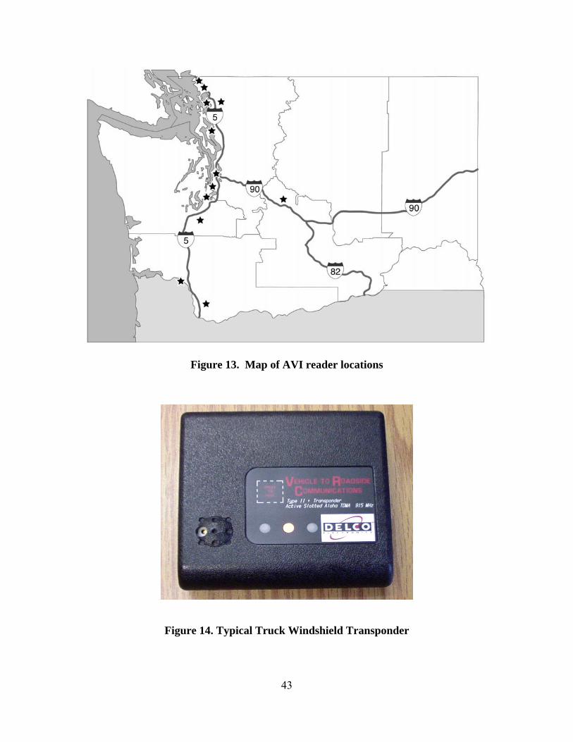
43
Figure 13. Map of AVI reader locations
Figure 14. Typical Truck Windshield Transponder

44
The transponders used as part Washington’s weigh-in-motion systems are
designed to promote the safe and legal movement of commercial vehicle traffic both in
Washington and throughout the country. This system is based within the national
Commercial Vehicle Information Systems and Networks (CVISN) program. Washington
was one of the original CVISN states and has a relatively well developed, and growing,
CVISN-based system. The CVISN weigh-in-motion transponder program allows trucks
to bypass weigh stations by electronically verifying a truck's weight and credentials as the
truck continues along the road at freeway speeds. The transponder is a short-range radio
communication device assigned to a specific vehicle and mounted on the inside of the
vehicle's windshield (Figure 14). It is used to electronically identify the truck, much like
an electronic license plate. The WIM system is embedded in the roadway about a half-
mile ahead of the weigh station and weighs a truck passing over it. At the same time, an
AVI device over the lane reads the transponder and checks various databases to verify the
truck's size, carrier registration, and safety record while the truck continues moving. The
AVI reader communicates electronically with the transponder and then activates a green
light on the transponder (giving the driver permission to keep going) or a red light (telling
the driver to pull in). For this research, CVISN truck tag reads could be obtained for
single or both directions (depending on the location) from WIM facilities on Interstate-5
at Ridgefield, Fort Lewis, Stanwood Bryant, and Bow Hill, and on Interstate-90 at Cle
Elum.
WSDOT’s three ongoing border data ITS also provide transponder reads that can
be used to obtain freight data. These border projects are designed to facilitate the
movement of participating commercial vehicles over the Washington/British Columbia

45
border by providing commercial vehicle operators, shipping lines, and border
enforcement agencies with electronic information about vehicles and their cargo. One of
these systems was designed to monitor and facilitate the movement of northbound trucks
carrying containerized in-bond freight over the Washington/British Columbia border.
This effort used the same transponder as used for the WIM system to monitor the
container, eventually record the container crossing into Canada, and automatically clear
out the bond. A similar system is being developed that will use transponders on trucks
hauling containers southbound out of British Columbia into Washington. As a result of
these systems, there are AVI readers at the exit gates of the American President Lines
terminal at the Port of Seattle, the Maersk terminal at the Port of Tacoma, and south- and
northbound at the Blaine Customs station at the Washington/British Columbia border.
TRANSPONDER ANALYSIS STEPS
Because truck transponders typically involve longer distance travel, the estimated
travel time from point to point could include stop times. Since the time spent stopped
would not be part of facility performance, the truck tags could only better represent the
facility’s performance if those trips with stops were not included in the estimation.
Therefore, to accurately estimate truck travel time using truck tags, a methodology was
needed to identify and remove those trips during which the driver stopped between
readers. The analysis process extracted useful truck travel time data (later converted to
average speed) from the truck transponders.
Converting truck tag travel time information into meaningful data was not simply
a matter of averaging the measured travel times. First, not all truck tags observed at
consecutive reader locations could be used for computing travel time because a truck

46
could exit before reaching the next reader or appear in the middle of the segment, and
thus not be recorded by the first reader. For example, Figure 15 shows that the average
daily number of usable tag reads for the several sections of northbound I-5. This ranged
from an average of 557 tag equipped trucks traveling between Ridgefield and Fort Lewis
to only 44 tag equipped trucks traveling between Ridgefield and Stanwood2. This
showed that the amount of usable data would decrease for longer routes (e.g. 557 vs. 44
matched data points).
Figure 15. Usable Truck Tags for Estimating Travel Time
2 This assessment was performed for the week of March 25, 2002.
Usable CVISN Truck Tags For Estimating Travel TimeDaily Average
557
7044
0
100
200
300
400
500
600
From Ridgefield to Fort Lewis From Fort Lewis to Stanwood From Ridgefield to StanwoodRoute
Num
ber o
f mat
ched
dat
a po
ints

47
The other concern was that we were measuring long distance travel (typically
greater than 100 miles between consecutive readers), and when traveling long distances,
drivers frequently stop for a variety of reasons (e.g., for a rest break or to drop off or pick
up cargo). In addition, given the long distances involved, a considerable difference can
exist in travel time from one vehicle to the next, simply as a result of minor variations in
how fast individual drivers choose to drive on a free flow road. Consequently, the
"average travel time" measured by truck tags would not really make a very good estimate
of either "how long it should take you" to drive this distance, or how well the road was
really performing. Therefore, vehicles that had stopped needed to be removed from the
"facility performance analysis." The algorithm developed for this project basically
identified outliers in travel times that had similar start times on the freeway segment
being monitored (e.g., tags with travel times far longer than tags that passed the first
reader at a similar start time). The same analysis approach was applied to data from both
WIM transponder and border tags.
Identifying Available Travel Times
The first step in the analysis process or "algorithm" is to identify the truck tags
that can be used for computing travel time. Not all truck tags observed at consecutive
reader locations can be used for computing travel time, because a truck can exit before
reaching the next reader or a truck can appear in the middle of the segment and therefore
not be recorded by the first reader.
This step is relatively easy to perform; trip travel times are computed from the
matched tags using time of arrival at two locations (e.g., T12 = TFort Lewis - TRidgefield) as a
function of trip start time (see Table 3).

48
Table 3. Matching Truck Tags
Tag ID WIM Site Time Travel Time 53 Ridgefield (MP 15) 00:26:44 53 Fort Lewis (MP 117) 02:31:19 02:04:35 75 Ridgefield (MP 15) 14:53:08 75 Fort Lewis (MP 117) 18:30:11 03:37:03 20801077 Blaine approach 12:35:31 20801077 Blaine exit 12:36:26
00:00:55
2088CD25 Port of Tacoma 19:50:28 03:45:29 2088CD25 Blaine approach 23:35:57 2088CD25 Blaine exit 23:37:44 00:01:47
The result is a preliminary data set that consists of all trucks that were detected at
both readers of a given segment. Trucks that were not detected at both readers of a
segment are taken out of the data set. This is done for each freeway segment (where a
segment is defined by two consecutive readers).
Identifying Best Available Travel Time
The next step is to identify which of the available truck data for a given freeway
segment will be used for freeway performance analysis. For each trip start time for a
segment, there may be several data points representing several trucks traveling on the
freeway segment at roughly the same time. These multiple data points for the same
5-minute trip start interval are converted into a single value by taking the fastest of those
segment speeds that is within the speed limit and using that value as the representative
value for that 5-minute interval. This is done for each 5-minute trip start time increment
for a given freeway segment. (Five minute was selected as the time interval because it
was reasonable frequent but still allowed for data aggregation.) This filtering step is

49
based on the assumption that if several trucks are all traveling on the same part of the
freeway at approximately the same time, the fastest of those trucks (traveling within the
speed limit) represents the best estimate of actual freeway performance, and the other
trucks are slower because of other reasons (driver preference, stops made, etc.). For
example, during a 5-minute interval from 5:15 to 5:20, although the average speed ranges
from 44 mph to 58 mph, the truck with an average speed of 58 mph would best represent
the truck speed within that 5-minute interval.
Removing Outliers
Once we have identified the best available estimate of freeway performance for
each 5-minute trip start interval (from the previous step), we next evaluate the resulting
values to determine which can be used as estimates of freeway performance, and which
should be filtered out. Specifically, only trucks that made non-stop trips between
consecutive reader locations can be used as an estimate of freeway performance on that
segment. Therefore, we wish to filter out data points that appear to represent trucks that
have made one or more stops while traveling between readers. To do this, we focus on
identifying sudden significant changes in segment travel time between trucks that are
traveling on the same freeway segment but at consecutive 5-minute trip start intervals.
The assumption here is that freeway performance ordinarily changes in a relatively
smooth manner within a short period (say ≤ 20 minutes or so), assuming there are no
blocking incidents, and that therefore the travel times of trucks traveling on the same
segment but only minutes apart should not be significantly different. A significant
difference would therefore indicate that the truck made one or more stops at some point
along the way while traveling on that freeway segment, thus adding to its trip time.
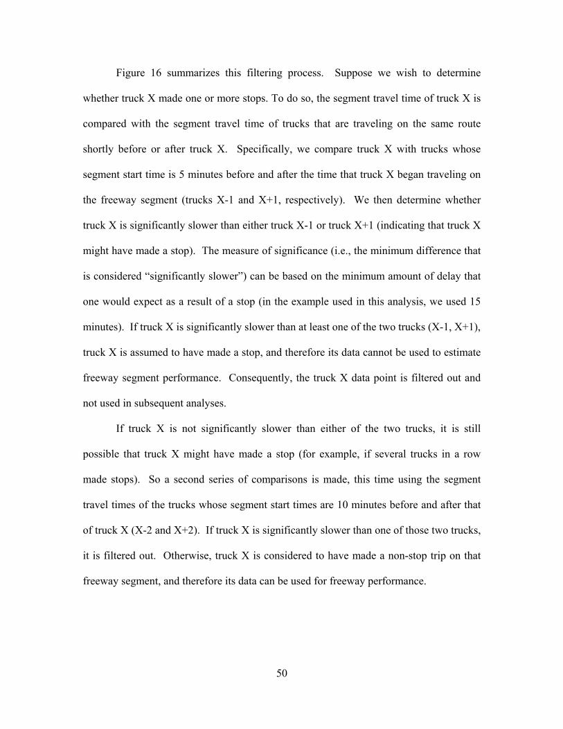
50
Figure 16 summarizes this filtering process. Suppose we wish to determine
whether truck X made one or more stops. To do so, the segment travel time of truck X is
compared with the segment travel time of trucks that are traveling on the same route
shortly before or after truck X. Specifically, we compare truck X with trucks whose
segment start time is 5 minutes before and after the time that truck X began traveling on
the freeway segment (trucks X-1 and X+1, respectively). We then determine whether
truck X is significantly slower than either truck X-1 or truck X+1 (indicating that truck X
might have made a stop). The measure of significance (i.e., the minimum difference that
is considered “significantly slower”) can be based on the minimum amount of delay that
one would expect as a result of a stop (in the example used in this analysis, we used 15
minutes). If truck X is significantly slower than at least one of the two trucks (X-1, X+1),
truck X is assumed to have made a stop, and therefore its data cannot be used to estimate
freeway segment performance. Consequently, the truck X data point is filtered out and
not used in subsequent analyses.
If truck X is not significantly slower than either of the two trucks, it is still
possible that truck X might have made a stop (for example, if several trucks in a row
made stops). So a second series of comparisons is made, this time using the segment
travel times of the trucks whose segment start times are 10 minutes before and after that
of truck X (X-2 and X+2). If truck X is significantly slower than one of those two trucks,
it is filtered out. Otherwise, truck X is considered to have made a non-stop trip on that
freeway segment, and therefore its data can be used for freeway performance.

51
Tx – Tx-2 = 2nd travel time backward Tx – Tx-1 = 1st travel time backward Tx = travel time of interest Tx – Tx+1 = 1st travel time forward Tx – Tx-2 = 2nd travel time forward Step 1 Tx – Tx-1 z 15 min Yes Yes No No
Tx – Tx+1 z 15 min Yes No Yes No
Exclude Exclude Exclude Continue to Step 2
Step 2 Tx – Tx-2 z 15 min Yes Yes No No
Tx – Tx+2 z 15 min Yes No Yes No
Exclude Exclude Exclude Include
Figure 16. Data Filtering Process
TESTING OUTPUT
The usefulness of the transponder data depended on having enough transponder
reads. Since the segments were defined by the location of WIM freight facilities, the
location of these segments were not necessarily what would have been selected for a data
program, and some segments might not be useful. Accuracy of the reads was also a
concern. In addition, the usability of the data might vary by time of day, week, and year.
WIM Transponders
Based on the analysis steps, Figure 17 shows the ones with the highest speed
within each 5-minute interval on the segment from Ridgefield to Fort Lewis. These are
also labeled as “unfiltered,” as they may contain trips with stops. Figure 18 illustrates the
filtered results based on the rules shown in Figure 16. Rolling hour averages are depicted
in Figure 19.

52
Avearge Truck Speed (max value for each 5-min interval)I-5 NB, Ridgefield to Fort Lewis (102 miles) Monday, 3/25/02
0
10
20
30
40
50
60
70
0:00:0
0
1:00:0
0
2:00:0
0
3:00:0
0
4:00:0
0
5:00:0
0
6:00:0
0
7:00:0
0
8:00:0
0
9:00:0
0
10:00
:00
11:00
:00
12:00
:00
13:00
:00
14:00
:00
15:00
:00
16:00
:00
17:00
:00
18:00
:00
19:00
:00
20:00
:00
21:00
:00
22:00
:00
23:00
:00
Time of Day
Truc
k Sp
eed
Figure 17. Average Truck Speed (5-Minute Interval) - Unfiltered
Avearge Truck Speed (max value for each 5-min interval) - FilteredI-5 NB, Ridgefield to Fort Lewis (102 miles) Monday, 3/25/02
0
10
20
30
40
50
60
70
0:00:0
0
1:00:0
0
2:00:0
0
3:00:0
0
4:00:0
0
5:00:0
0
6:00:0
0
7:00:0
0
8:00:0
0
9:00:0
0
10:00
:00
11:00
:00
12:00
:00
13:00
:00
14:00
:00
15:00
:00
16:00
:00
17:00
:00
18:00
:00
19:00
:00
20:00
:00
21:00
:00
22:00
:00
23:00
:00
Time of Day
Truc
k Sp
eed
Figure 18. Average Truck Speed (5-Minute Interval) - Filtered

53
Avearge Truck Speed (rolling hour) - FilteredI-5 NB, Ridgefield to Fort Lewis (102 miles) Monday, 3/25/02
0
10
20
30
40
50
60
70
0:00:0
0
1:00:0
0
2:00:0
0
3:00:0
0
4:00:0
0
5:00:0
0
6:00:0
0
7:00:0
0
8:00:0
0
9:00:0
0
10:00
:00
11:00
:00
12:00
:00
13:00
:00
14:00
:00
15:00
:00
16:00
:00
17:00
:00
18:00
:00
19:00
:00
20:00
:00
21:00
:00
22:00
:00
23:00
:00
Time of Day
Truc
k Sp
eed
Figure 19. Average Truck Speed (Rolling Hour)
Border Transponders
This study found that only the tag reads collected at the Blaine border could be
used for further analysis. The reads from the ports could not be used because of
problems with spatial and temporal data coverage (this will be discussed later).
Figure 20 shows an example of the truck tag reads converted into time durations
for trucks traveling northbound on a half-mile segment from H Street (e.g., approaching
the border) to the duty free shop (e.g., near the end of freeway leading to the Canada
Customs). The duration information could potentially be used to gauge delay conditions
near the border area before Canada Customs. However, because the truck travel patterns
can include one of the following: (1) heading directly to Canada Customs without

54
Blaine (approach-exit)Tuesday, 7/16/2002
163 Data Points
0:00:00
0:15:00
0:30:00
0:45:00
1:00:00
1:15:00
1:30:00
0:00 1:00 2:00 3:00 4:00 5:00 6:00 7:00 8:00 9:00 10:00
11:00
12:00
13:00
14:00
15:00
16:00
17:00
18:00
19:00
20:00
21:00
22:00
23:00
0:00
Start Time
Dur
atio
n
Figure 20. Duration near the Border – Unfiltered data
stopping or (2) stopping in a nearby parking lot to process U.S. brokerage paperwork and
then heading to Canada Customs, a prolonged time duration may be interpreted as a
result of “border delay” (e.g., as a result of vehicle volumes and processing rates at the
booth) and/or time taken to process U.S. brokerage paperwork.
To some extent, if there are adequate data points, we can identify sudden
significant changes in segment travel time between trucks that are traveling on the same
freeway segment. The assumption here is that freeway performance ordinarily changes
in a relatively smooth manner within a short period (say ≤ 20 minutes or so); therefore,
the travel times of trucks traveling on the same segment but only minutes apart should
not be significantly different. A significant difference would indicate that the truck made
a stop to process U.S. brokerage paperwork, thus adding to its trip time.

55
For example, if truck X with a start time of 20:30, shown in Figure 20, is
significantly slower than other trucks that start within 20 minutes before and after truck X
(e.g., 50 minutes vs. less than 30 minutes), it is considered to have made a stop before it
entered the Canada Customs. Figure 21 shows filtered results based on this approach.
Notice that adequate data reporting frequency is essential for verifying data filtering
logic.
DATA LIMITATIONS
The method of eliminating nonapplicable travel time assumes frequent data points
to allow data verification (e.g., every 5 to 15 minutes). The methodology does not work
well for a dataset that has wide time gaps because trips with longer gaps produce more
uncertainties.
Blaine (approach-exit)Tuesday, 7/16/2002
163 Data Points
0:00:00
0:15:00
0:30:00
0:45:00
1:00:00
1:15:00
1:30:00
0:00 1:00 2:00 3:00 4:00 5:00 6:00 7:00 8:00 9:00 10:00
11:00
12:00
13:00
14:00
15:00
16:00
17:00
18:00
19:00
20:00
21:00
22:00
23:00
0:00
Start Time
Dur
atio
n
Figure 21. Duration near the Border – Filtered Data

56
Spatial Data Coverage
Unlike traffic management system data that cover a much smaller geographic
urban area and have a more dense sensor network (e.g., loop data at about a ½-mile
interval), the truck tags usually represent long segments (e.g., 100 or more miles per
segment) that traverse both urban and rural areas. For example, Ridgefield and Stanwood
are about 200 miles apart, with Fort Lewis roughly midway between; the truck border is
about 110 miles north of the Port of Seattle and 140 miles from the Port of Tacoma. Less
information is obtainable with low sensor density on longer routes. Route diversion may
occur more frequently on long segments, resulting in fewer matched tag reads.
Figure 22 shows that more than 1,000 CVISN truck tags are observed on a typical
weekday at both Ridgefield and Fort Lewis, but Stanwood Bryant has about 400 tag
reads. On weekends, the number of truck tag reads can decrease about 60 percent.
Fewer trucks traveling from Fort Lewis pass through Stanwood; many trucks may have
already reached their destination, such as Seattle, before reaching Stanwood. Also, a
rough estimate depicted in Figure 15 shows that with the greater the distance between
readers, there will likely be fewer matched data points for travel time. Many more
matched tag reads are available for the segment from Ridgefield to Fort Lewis than for
the other segments (24 vs. 3 trucks per hour).3 This suggests that a significant number of
trucks originating in Ridgefield may have diverted to other routes (or have already
reached their destination such as Seattle) before reaching Stanwood. Less than 5 percent
of the tags from Ridgefield can be used.
3 This analysis captures the majority of the truck trips but omits a small percentage of trips that start near mid-night and pass through the end reader the next morning.

57
Frequency of Truck Tag Reads
1258
1007
381
468
366
124
Ridgefield Fort Lewis Stanwood Bryant
Weekday Average Weekend Average
Figure 22. Frequency of Truck Tag Reads
Temporal Data Coverage
Figures 23 through 25 show the distribution of the time gap between trucks.
Truck traffic from Ridgefield to Fort Lewis is relatively frequent; a travel time can be
reported as often as every 5 minutes or less 90 percent of the time. On the other hand,
reportable truck travel times are much less frequent for trips from Fort Lewis to
Stanwood Bryant. Fewer than half of the trips are 5 minutes apart or less. The gap is
even greater for longer segments. Half of the trucks traveling from Ridgefield to
Stanwood Bryant are at least 20 minutes apart. In fact, one out of five truck travel times
is generated every 40 minutes or longer. More uncertainty is introduced when a slow trip
is bound by faster speeds within 40 minutes than by 15 minutes.

58
Time Gap between Each TruckI-5 NB, Ridgefield to Fort Lewis (102 miles)
0%
20%
40%
60%
80%
100%
1 5 9 13 17 21 25 29 33 37 41 45 49 53 57 61 65
Number of Miniutes between Each Truck
Perc
enta
ge
Figure 23. Gap between Trucks, Ridgefield to Fort Lewis
Time Gap between Each TruckI-5 NB, Fort Lewis to Stanwood Bryant (98 miles)
0%
20%
40%
60%
80%
100%
1 5 9 13 17 21 25 29 33 37 41 45 49 53 57 61 65
Number of Miniutes between Each Truck
Perc
enta
ge
Figure 24. Gap between Trucks, Fort Lewis to Stanwood Bryant

59
Time Gap between Each TruckI-5 NB, Ridgefield to Stanwood Bryant (200 miles)
0%
20%
40%
60%
80%
100%
1 5 9 13 17 21 25 29 33 37 41 45 49 53 57 61 65
Number of Miniutes between Each Truck
Perc
enta
ge
Figure 25. Gap between Trucks, Ridgefield to Stanwood Bryant
Table 4. Frequency of Data Points
Number of Data Points Sample Week Border crossing Port of Seattle to the
truck border in Blaine Port of Tacoma to the truck border in Blaine
Monday 133 2 1 Tuesday 163 6 4 Wednesday 184 1 5 Thursday 158 2 1 Friday 184 4 2 Saturday 88 0 0 Sunday 16 0 0

60
Although there are relatively frequent tag reads at the border, not many of them
are available for tracking from either the Port of Seattle or the Port of Tacoma. Less than
5 percent of the truck tags identified at the border come from either ports. A one-week
sample indicates the problems of low data frequency for the route from the ports to the
border (see Table 4). Therefore, given the limited number of data points on the I-5 and
SR 543 corridors from the Port of Tacoma and Seattle to the Blaine truck border, it is
impossible to perform a valid analysis.
With long distance travel, the estimated travel time from point to point is more
likely to include stop times. When adequate numbers of data are available, data can be
processed to identify and remove trips during which the driver stopped between readers.
For example, if all four trucks that leave within 10 minutes from each other around 4:00
PM on July 16, 2002, from the Port of Tacoma have similar travel times (see figures 26
and 27), then there is more information to support the assertion that the delay is due to
traffic congestion.
On the other hand, if data points are sparse, then it is difficult to determine
whether a data point in question is usable. For example, a truck leaving from the Port of
Seattle around 5:30 PM on July 19, 2002 (see Figure 28), takes 2 hours and 35 minutes to
get to the border (which is equivalent to an average trip speed of 44 mph, as illustrated in
Figure 29), about a half hour longer than traveling under free flow conditions (the trip
should take about 2 hours or less). Since Figure 28 shows that the closest data point is a
truck that left one hour before, and no other data points are available, it is not possible to
determine whether the half hour delay is caused by a rest stop or traffic congestion.

61
Port of Tacoma to Truck Border (142 miles)Week 7/15/2002 - 7/21/2002
0:00:00
0:30:00
1:00:00
1:30:00
2:00:00
2:30:00
3:00:00
3:30:00
4:00:00
4:30:00
19:50
:28
20:32
:48
16:03
:43
16:12
:17
16:12
:19
16:12
:20
18:14
:29
21:01
:17
18:54
:22
20:18
:02
20:39
:19
1:14:0
7
2:12:1
1
15:59
:51
16:03
:39
Trip Start Time
Dur
atio
nPort of Tacoma to Blaine Approach Blaine Approach to Exit
7/15/02
7/17/02
7/18/02
7/19/027/16/02
Figure 26. Port of Tacoma to Border: Sample Travel Time
Port of Tacoma to Truck Border (142 miles)Week 7/15/2002 - 7/21/2002
0
10
20
30
40
50
60
70
19:50
:28
20:32
:48
16:03
:43
16:12
:17
16:12
:19
16:12
:20
18:14
:29
21:01
:17
18:54
:22
20:18
:02
20:39
:19
1:14:0
7
2:12:1
1
15:59
:51
16:03
:39
Trip Start Time
Ave
rage
Trip
Spe
ed
0:00:00
0:51:26
1:42:51
2:34:17
3:25:43
4:17:08
5:08:34
6:00:00
Tim
e D
urat
ion
Spen
t at t
he B
orde
r
Port of Tacoma to Blaine Approach (average trip speed) Blaine Approach to Exit (time duration)
7/15/02 7/17/02 7/18/02 7/19/027/16/02
Figure 27. Port of Tacoma to Border: Sample Speed

62
Port of Seattle to Truck Border (114 miles)Week 7/15/2002 - 7/21/2002
0:00:00
0:30:00
1:00:00
1:30:00
2:00:00
2:30:00
3:00:00
3:30:00
4:00:00
4:30:00
16:35:11 15:49:57 18:04:53 20:46:29 20:57:35 16:31:42 17:03:22 17:45:00 18:42:53 20:30:23 18:47:08 16:28:24 17:27:09
Trip Start Time
Dur
atio
nPort of Seattle to Blaine Approach Blaine Approach to Exit
7/15/02
7/17/027/18/02
7/19/027/16/02
Figure 28. Port of Seattle to Border: Sample Travel Time
Port of Seattle to Truck Border (114 miles)Week 7/15/2002 - 7/21/2002
0
10
20
30
40
50
60
70
16:35:11 15:49:57 18:04:53 20:46:29 20:57:35 16:31:42 17:03:22 17:45:00 18:42:53 20:30:23 18:47:08 16:28:24 17:27:09
Trip Start Time
Ave
rage
Trip
Spe
ed
0:00:00
0:51:26
1:42:51
2:34:17
3:25:43
4:17:08
5:08:34
6:00:00
Tim
e D
urat
ion
Spen
t at t
he B
orde
r
Port of Seattle to Blaine Approach (average trip speed) Blaine Approach to Exit (time duration)
7/15/02 7/17/02 7/18/02 7/19/027/16/02
Figure 29. Port of Seattle to Border: Sample Speed

63
CONCLUSIONS ABOUT THE USE OF TRANSPONDER DATA
The analysis of currently collected tag data described above illustrates the current
limitations in the use of CVISN truck tags along with the limited number of reader
locations currently available to WSDOT. The long segment lengths being monitored and
the fact that many truckers stop at some point (for fuel, to rest, to drop off or pick up
loads), means that a reasonably large number of tag observations are needed at each
location in order to compute travel times with reliability. Only one of the segments being
monitored currently have sufficient CVISN tag matches to produce reliable real-time
truck travel time matches. This is the Ridgefield to Ft. Lewis segment.
The other segments tested, such as Ft. Lewis to Stanwood-Bryant and the Seattle
and/or Tacoma Port gates to the Canadian Border segments, lack sufficient truck tag
volumes to differentiate between travel times effected by congestion and those affected
by voluntary truck stops.
The Ft. Lewis to Stanwood segment suffers from the fact that most CVISN tag
equipped trucks coming from the south appear to stop in the Seattle/Tacoma metropolitan
region. Thus, while the number of tag reads at Ft. Lewis is high, the number of tag reads
at Stanwood is moderately low, and the number of actual tag matches is low. On the
other hand, the computation of travel times between the two ports and the Canadian
border is limited by a very low number of tags being read at the two ports.
The project data analysis does indicate that it may be possible to produce planning
level estimates of the “expected” travel times for freight on all of these movements, by
time of day, and day of week. It may also be possible to determine the frequency of
congestion on some of these routes. However, without a considerable increase in the
number of tag reads that occur at the port itself, it is unlikely that the travel time to the

64
Canadian border from the ports can be accurately measured. This may require placement
of a tag reader at the primary freeway ramps leading away from the ports.
Still, while the data analysis shows that this technique does not provide all of the
data hoped for, it does show that the technique holds considerable promise, especially
with the expected increase in both the number of trucks carrying tags, and the number of
tag readers on key Washington highways. Thus, the project team believes that this effort
should continue. Future efforts in this area should include:
• obtaining more data points by increasing sensor density,
• continue to refine the algorithm used for filtering measured travel times,
• explore what type of information should be given to the public about
travel times on these corridors, and
• look for opportunities to integrate these data with other types of travel
data, to both enhance the level of information available, and to see if other
data sources can limit some of the weaknesses of these data.

65
4. FLOW SYSTEM DATA
The last major source of data examined within this project is the traffic
surveillance system data collected by WSDOT’s Puget Sound area freeway surveillance
and control system (known as FLOW). The FLOW surveillance system consists of over
3,000 loop detectors (located at more than 300 basic sites), over 160 CCTV cameras, and
a small number of other detectors, including radar detectors and magnetometers. The
data collected are used to operate the WSDOT’s ramp metering system, as well as for
managing reversible roadway operations, incident response, and construction traffic.
The facilities that are covered by the loop system are shown in Figure 30. The
geographic coverage of the system is expanding slowly. For the most part, surveillance
system coverage expands whenever WSDOT performs a capacity expansion project.
Recently, these have been expansions of the HOV lane system.
The primary “data collection” devices used within FLOW are loop detectors.
FLOW uses both single and dual loop installations. The loops report vehicle volumes
and lane occupancy statistics every 20 seconds. In addition to these statistics, dual loops
also report average vehicle speeds. Loops are located in both mainline and ramp
locations. Mainline loops provide information on roadway volume flow, traffic density
(estimated on the basis of volume and lane occupancy), and roadway speed. (For single
loops, volume and occupancy are converted into speed estimates by using an assumed
average vehicle length. For dual loops, speed can be directly computed for each vehicle
observed on the basis of the time difference in loop activations at consecutive loop
installations.)

66
Figure 30. Freeway Surveillance System Coverage

67
In theory, dual loops can also provide estimates of vehicle volumes, disaggregated
into one of four length bins. Unfortunately, tests of the current truck counts indicate that
these counts are not accurate. WSDOT is researching ways to make these counts more
accurate.
A significant percentage of the loops are located on freeway ramps rather than on
the freeway mainline. Off-ramp detectors provide a measure of ramp utilization. On-
ramp detector data not only measure usage, but also provide key control system inputs to
the ramp metering algorithm. Each on-ramp can contain as many as four loops for each
ramp lane. Loops are located at
• the ramp meter stop bar (where they act as a demand indicator)
• just past the stop bar (where they serve as a passage indicator, meaning
that they measure when a vehicle has left the stop bar)
• upstream of the stop bar (where they act as queue detectors)
• at the arterial at the top of the ramp, (where they serve as advance queue
detectors, meaning the ramp queue has grown large enough to hamper
arterial operations).
Data from these various loop are used as inputs in the ramp metering algorithm to
judge the size and impact of ramp queues, and combined with mainline loop data, they
can be used to determine whether vehicles are being stored on the freeway mainline.
The 20-second loop detector data are saved in an archive operated by the
University of Washington’s ITS Program and are available on the Internet via the website
http://www.its.washington.edu/tdad/tdad_top.html. The 20-second data are also
aggregated to 5-minute totals and saved in an archive maintained by WSDOT. These

68
data can be obtained from WSDOT on a compact disk (CD). An entire year of data for
all loops requires four disks.
FLOW DATA ANALYSIS
WSDOT has developed an extensive analysis process that converts the archived
loop data into performance statistics. Performance statistics are reported routinely by
WSDOT both as part of the quarterly Grey Notebook4 and as part of two biennial
performance reports, The HOV Lane Performance Monitoring report5 and the Central
Puget Sound Freeway Network Usage and Performance report.6 Copies of both reports
are available through the TRAC web site at http://depts.washington.edu/trac/.
The extensive geographic and temporal coverage of the FLOW surveillance
system allows these performance reports to provide significant detail in the operational
performance of the freeway system. This allows analysts to understand geographic
location, scope, duration, and intensity of congestion. These statistics can then be used to
examine the cost to freight movements of freeway congestion.
The current analytical procedures (called CD Analyst) allow the Department to
examine the geographic nature of traffic, both as an average condition and as a frequency
of occurrence. Figure 31 illustrates the average facility performance of the northern
portion of Interstate 5. This figure shows the two directions of travel independently and
uses colors to describe average condition. (These graphics are based on the mean lane
occupancy for all freeway loop detectors for all weekdays for 1999. Color codes are
selected on the basis of the basic relationship between lane occupancy and traffic density,
4 http://wsdot.wa.gov/accountability/GrayNotebook.pdf 5 http://depts.washington.edu/trac/bulkdisk/pdf/506.1.pdf 6 http://depts.washington.edu/trac/bulkdisk/pdf/493.1.pdf

69
and ultimately level of service.) Essentially, green means very good conditions are
routinely found at a given time and place, while yellow means free flowing but fairly
dense traffic is common. Red means congestion is frequent, while blue means congestion
is very common and likely severe. A traveler’s “average” trip can also be simulated by
passing through this graphic diagonally. (In the southbound direction, use the left hand
image and travel top to bottom, left to right. For the northbound direction travel bottom
to top, left to right.)
Figure 32 shows a slightly different version of this same geographic view of
congestion. The difference is that while Figure 31 shows “average condition,” Figure 32
shows the frequency with which LOS F conditions occur during weekdays.
Time
Mile
post
0 2 4 6 8 10 12 2 4 6 8 10 12Time
Mile
post
0 2 4 6 8 10 12 2 4 6 8 10 12AM PM AM PM
174
188
186
184
182
180
178
176
174
188
186
184
182
180
178
176
Uncongested, near speed limit
Restricted movement but near speed limit
More heavily congested, 45 - 55 mph
Very congested, unstable flow
Snohomish County King County
NE 175th
405
5
526
99
128th St
NE 145th
NE Northgate Way
NorthboundSouthbound
N
Interstate 5 North Traffic Profile General Purpose Lanes 1999 Weekday Average
Figure 31. Average Operating Condition of I-5 By Time of Day and Location

70
Mile
post
0 2 4 6 8 10 12 2 4 6 8 10 12Time
0 2 4 6 8 10 12 2 4 6 8 10 12Time
Mile
post
AM PM AM PM
165164163162161160159158157156155154153
166167168169170171172173
165164163162161160159158157156155154153
166167168169170171172173
Spokane St.
Albro Pl.
90
5
Marion St.
Boeing Access Rd.
405
599
518
520
522
NE Northgate Way
NorthboundSouthbound
N
Congested weekdays per week
0 to 1 day 1 to 2 days 2 to 3 days 3 to 4 days 4 to 5 days
Interstate 5 South Congestion Frequency General Purpose Lanes 1999 Weekday Average
Figure 32. Frequency of LOS F Congestion on I-5
Both graphics allow an analyst to determine where congestion routinely occurs,
how far geographically that congestion extends, and how long it lasts. Problem locations
can then be examined in detail.
Figure 33 shows one graphic (and set of performance measures) that can be used
to examine a specific problem location. This graphic illustrates, by time of day, the
average vehicle volume being carried by general purpose lanes at a given location (the
colored line, read on the left-hand axis); the average speed those vehicles are traveling
(the color of the line itself, where green is 55+ mph, red is below 45 mph, and yellow is
between 45 and 55 mph); and the frequency with which that location experiences LOS

71
Figure 33. Location Specific Volume, Average Speed, and Frequency of Congestion
Figure 34. Use of Location Specific Graphics To Examine Performance Trends
SR-520 76th Ave NE GP WB
0
500
1000
1500
2000
2500
12 AM 2 AM 4 AM 6 AM 8 AM 10 AM 12 PM 2 PM 4 PM 6 PM 8 PM 10 PM
Vehi
cles
Per
Lan
e Pe
r Hou
r (VP
LPH
)
0
10
20
30
40
50
60
70
80
90
100
Con
gest
ion
Freq
uenc
y (%
)
Estimated Weekday Volume, Speed, and Reliability Conditions (1999)
Volume and Congestion on Eastbound SR-520 on the Viaduct
0
10
20
30
40
50
60
70
80
90
5:30 AM 7:30 AM 9:30 AM 11:30 AM 1:30 PM 3:30 PM 5:30 PM 7:30 PMTime of Day
Freq
uenc
y of
Con
gest
ion
0
200
400
600
800
1000
1200
1400
1600
1800
2000H
ourly
Vol
ume
Per L
ane
(vpl
ph)
2001 Congestion1999 Congestion2001 Volume1999 Volume
170 veh / hr / ln improvement
LOS F occurs 1 day per week less often

72
congestion (the blue histogram, read against the right-hand axis). These statistics can
then be tracked over time (as illustrated in Figure 34) to show how facility performance is
changing as a result of growth in the area and the implementation of new operational
control and incident response strategies.
By analyzing data for individual days for all locations on a freeway corridor, it is
also possible to compute “virtual travel times” on the freeway by time of day. These
virtual travel time runs can then be summarized for all days of interest to provide yet
another excellent performance measure, illustrated in Figure 35. This figure shows mean
travel times for a specific trip in 1999, along with the 90th percentile travel time required
for that trip. This type of analysis is particularly useful for understanding the effects of
congestion on schedule adherence and labor utilization for freight, because it provides a
direct measure of the variation in trip times. The variation of trip times allows analysis of
the effects of congestion frequency and duration on vehicle and labor scheduling for both
the freight and transit industries.
These same travel time statistics can also be used to determine the number of
times specific travel time performance standards are met or fail to be met. For example,
WSDOT uses virtual travel time statistics to monitor the performance of its HOV lane
system. A WSDOT policy is to maintain HOV lane performance at 45 mph or better, 90
percent of the time. Figure 36 illustrates how virtual travel times are used to report where
a given corridor is meeting these performance criteria.
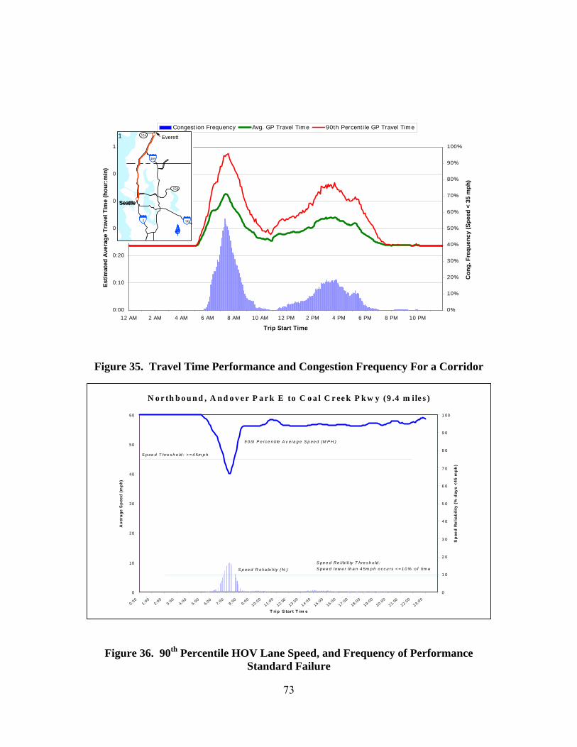
73
0:00
0:10
0:20
0:30
0:40
0:50
1:00
12 AM 2 AM 4 AM 6 AM 8 AM 10 AM 12 PM 2 PM 4 PM 6 PM 8 PM 10 PM
Trip Start Time
Est
imat
ed A
vera
ge T
rave
l Tim
e (h
our:
min
)
0%
10%
20%
30%
40%
50%
60%
70%
80%
90%
100%
Con
g. F
requ
ency
(Spe
ed <
35
mph
)
Congest ion Frequency Avg. GP Travel Time 90th Percentile GP Travel Time
405
90
5
520
526
N
SeattleSeattleSeattle
5
Everett1
Figure 35. Travel Time Performance and Congestion Frequency For a Corridor
Figure 36. 90th Percentile HOV Lane Speed, and Frequency of Performance Standard Failure
N o r th b o u n d , A n d o v e r P a r k E to C o a l C r ee k P k w y (9 .4 m ile s )
0
10
20
30
40
50
60
0:001:00
2:003:00
4:005:00
6:007:00
8:009:00
10:0011:00
12: 00
13:0014:00
15:0016:00
17:0018:00
19:0020:00
21: 00
22:0023:00
T ri p S tar t T im e
Ave
rage
Sp
eed
(mph
)
0
1 0
2 0
3 0
4 0
5 0
6 0
7 0
8 0
9 0
1 00
Sp
eed
Rel
iabi
lity
(% d
ays
<45
mph
)S p ee d T hre s h o ld : > = 4 5m p h
S pe e d R e l ibi l i ty T hre s h o ld : S pe e d low e r th a n 4 5m p h o c c u rs < = 1 0 % o f tim e S p ee d R el ia bi l i ty (% )
9 0 th P e rc e n ti le A v era g e S p ee d (M P H )

74
CONCLUSIONS
The use of FLOW data for performance analysis is extremely powerful.
However, it does have several significant limitations. The biggest of these limitations is
that data are available only for a limited set of roadways, and the cost of surveillance
system expansion means that additional data collection only occurs as part of the
expansion of the WSDOT’s surveillance and control system. A second, and somewhat
less important limitation, is that the large size of the data archive creates some significant
data handling and quality control problems. These can be surmounted with effort and
funding resources. Finally, as was pointed out in Chapter 2 of this document, the
performance of heavy trucks appears to be worse than the “average” condition reported
by the FLOW system statistics. Thus, care must be taken when using these statistics as a
direct measure of truck performance.

75
5. INTEGRATION OF DATA SETS
As discussed in the previous sections, different ITS systems generate data that
have different characteristics. Those data can present differing pictures (versions) of
freight flow performance for the same stretch of roadway. In addition, ITS data often
cover different (and non-contiguous) roadway segments and systems or geographic areas.
The result of this wide variety is an integration task that is far more complex that might
be initially expected. That integration task, however, is often worth the effort needed to
combine and use these data. Integration of data from the entire range of ITS devices
potentially offers both a more complete and more accurate overall description of freight
and truck flows.
The results of the work described in the first four chapters of this report have
indicate that the collection and integration of ITS data is worthwhile. This chapter
discusses the work required to achieve that integration. The chapter starts with a
discussion of some of the broader issues that must be dealt with for integrating ITS data.
It then transitions into a brief introduction to the preliminary design of an integration
system that WSDOT will construct to manage and make the ITS data it collects useful
and accessible to a wide variety of users.
DATA ACQUISITION
The first step in using data from ITS devices is simply acquiring the data. This
requires that the agencies that operate the Intelligent Transportation System actually
archive the data generated by the ITS devices. A large number of Intelligent
Transportations Systems do not currently archive and use the data they collect. This

76
occurs both because data archiving cost money, and because the storage and use of some
ITS data raise privacy concerns. In many cases, ITS operators have yet to clearly
recognize the significant benefits that can be gained from the use of data archives.
Financial and Organizational Cost
Data acquisition “costs” are both financial and organizational. The initial cost
identified is simply the cost associated with the computer hardware and software needed
to collect and store the data used by the ITS. This task is often of low importance to the
group that constructs and uses the ITS because the data are frequently used “in real time”
to make control and operational decisions. The operators, concerned with “today’s
crisis,” frequently have not investigated how the use of archived data can improve their
response to “today’s crisis.” The result is that the builders of the system see the archiving
of collected data as a “cost that can be removed from the system” (by not doing it), rather
than as a tool that allows them to make better decisions and perform their operational
tasks more efficiently.
Finding the funding to store and use ITS data is often made more difficult because
many of the intended uses for ITS data extend far beyond the reason the data were
initially collected. A good example of this is the conversion of toll tag data into travel
time estimates. The data are most typically collected as part of a revenue collection
function. However, these same data allow computation of both real-time travel time
estimates (which can be used for traveler information purposes) and historical facility
performance information that can be used for planning purposes. (In this case, planning
benefits include items such as determining on the basis of historical trends, the number of
staff needed by time of day and day of year, computing facility performance statistics for
the planning of future operational improvements, or the computation of vehicle speed

77
estimates that can be used as input to analyses such as air pollution emission estimates for
environmental reviews.)
While multiple uses of a single data source creates an “opportunity” for saving
money, those secondary users of the data are often within a different division of the
organization and obtain their funding from different “internal pots.” Satisfying their data
needs is likely to be of low importance to the organization that funds the initial ITS
system implementation and its ongoing operation. (For example, the Operations Division
may build and install a freeway surveillance system, but the Planning group could be a
key user of an archive of the surveillance data.) Consequently, the group that “funds” the
ITS data collection has little interest in funding methods to make those data useful for
others. They see this activity as a cost with little direct return on “their” investment.
This discrepancy of who pays and who gains is especially crucial when the archiving
effort (which includes but is not limited to the data storage, manipulation, and quality
control procedures discussed below) is perceived to have only a minor benefit to the
primary user.
While funding may be available from the “secondary” user of the ITS data (e.g.,
Planning can provide Operations with funding to perform the necessary tasks), this
requires levels of inter-departmental cooperation that are often difficult to achieve. The
secondary use of data also tends to highlight issues about data accuracy and completeness
that do not exist when only one group uses the data. An example of this is the fact that an
Operations group may not care that one of four lanes of loop detection has failed. When
used by the Operations group to estimate average facility speed at that location, the
remaining three sensors provide an acceptable level of accuracy in the collected data.

78
However, this same data availability condition may not be sufficient for some planning
purposes; for example, where facility volume must be accurately measured. In this case,
the loss of one sensor may prohibit the estimation of volume within the desired accuracy
limits.
Under this example condition a cost (fixing the broken sensor) is “unnecessary”
for the Operations group, but “important” to the Planning group. Not only is there likely
to be disagreement over who should pay for that repair, but there is likely to be
disagreement over how quickly the failed sensor needs to be identified and repaired.
Thus, differences in uses for the data and the various roles each agency
department or division plays in generating or using the data can cause tension in several
areas related to collecting the data. All of these types of issues create non-monetary
“costs” that complicate and hinder the creation and use of ITS archives.
Privacy
The second major stumbling block to use of ITS data revolves around concerns
about privacy. Many ITS identify specific vehicles. Use of these data for secondary
tasks raises concern that the privacy of the individuals associated with those vehicles may
be violated.
In some cases, privacy issues can be addressed by the use of encryption or
conversion (“anonymization”) of tag IDs prior to data storage. In other cases, restrictions
must be placed on the use of data that contain private information. Setting up formal
terms of use and privacy statements is an effective way to help limit privacy concerns.
79
DATA MANIPULATION AND QUALITY ASSURANCE
Once the data are acquired, they must be checked for validity and placed into
common data formats. One of the key tasks in the quality assurance effort is to correctly
assign tag and GPS data to the roadway network. In many cases, this process will use
GIS technology. The effectiveness of the GIS, in turn, is based on the availability of a
digital base map with appropriate spatial accuracy and an up-to-date and maintained road
network. Maintaining the GIS is often an additional cost not initially considered when an
archive that uses an existing ITS data source is developed. Once an accurate digital base
map has been provided, the GIS can be used for map matching, which is the process of
assigning the GPS or AVI sensor locations to a roadway. This step is particularly
important when using GPS data because it is the key to determining the actual travel path
(roads used) of the vehicle being monitored. (For example, is the vehicle going
moderately slowly because it is on a congested freeway, or is it simply traveling at the
posted speed limit on the arterial that is parallel to that freeway?)
Updated GIS maps are also of concern when location referencing systems other
than GPS are used by ITS. For example, many ITS use linear referencing systems such
as state route and milepost referencing schemes as their key location identifiers.
Correctly locating these devices within the GIS, and describing the links for which data
are valid, are key to integrating varied data sets with GIS. Other potential issues of
concern with the base map are an appropriate level of generalization and compatible map
projections.
The next issue to be addressed when combining data from different ITS is time.
Different ITS report data at different time intervals. For example, GPS vehicle location
data may be reported from every 2 seconds to every 3 minutes, while freeway operations

80
loop data for a given location may be reported from between every 20 seconds to every
15 minutes. Integrating these different data require accurate time stamps (and consistent
time baselines), as well as accurate locations. Integrating time stamps can be further
complicated by issues such as the base time period being used by the reporting system.
(Does it report times based on Greenwich Mean Time, Eastern Standard Time, or Pacific
Daylight Time?) Misunderstanding the time period used can lead to erroneous
calculations of speed and travel time. Other “time” issues can surface when changes
from daylight savings time to standard time occur differently.
Lastly, it is important to note that in many cases two ITS data collection systems
can develop “similar but different” data items. It is very important that these differences
be clearly identified as part of any integration effort because these “different” data items
can lead to questions about the accuracy of the data being collected. An example of this
phenomenon, presented in Chapter 2, is that the GPS data obtained from trucks raised
questions about the accuracy of the FLOW surveillance data. While both ITS efforts
provided “valid” measures of freeway speed, the output of the two systems was very
different. Careful analysis showed that “truck speed” was not the same thing as “average
roadway speed,” even though the two data sets used the same basic units (miles per hour)
and covered the same roadway segments.
If the “integrated system” did not fully explain the differences in the two data
sets, users of that system would question the validity of the two datasets. They could also
easily select the “wrong” statistic for use in their analysis. In the “truck speed” example
above, the “truck speed” estimate is a poor estimate of the facility performance that
would be experienced by most users of the road. Similarly, the “FLOW average facility

81
speed” under-estimates the speeds actually attained by heavy trucks on congested urban
freeways.
The solution to many of the “problems” noted above centers on the availability of
meta-data. The term meta-data is defined as “data about data.” Meta-data describe the
data from any given data source. Each ITS data archive needs a complete set of meta-
data. Clear, complete meta-data provide the information necessary for software
engineers, programmers, and analysts to develop and code the procedures necessary to
correctly integrate data from disparate sources. They also provide potential users with
the information they need to determine whether the data provided by a specific source (or
combination of sources) can meet their needs.
A DESIGN FOR INTEGRATING ITS DATA
The research team for this project determined that data storage for an ITS archive
can be provided by any type of computer system that meets the basic storage, access, and
reporting requirements of the archive. The project team selected GIS technology for
integrating the independent archives. GIS provides the best method for reconciling the
various geographic referencing systems used by GPS devices, AVI tags, and traffic
control system loops. The GIS provides an excellent user interface capability that allows
design of a system that can effectively inform potential data users of what data exist and
the relative location of those data collection points (or the geographic extent of specific
roadway segment performance measures).
However, rather than using the GIS to store all data collected within each of the
ITS archives, the project team determined that only summary statistics will be transmitted
into the integrated GIS archive. (Note that the GPS-based vehicle tracking system will
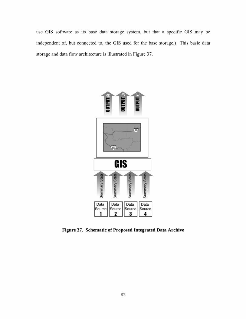
82
use GIS software as its base data storage system, but that a specific GIS may be
independent of, but connected to, the GIS used for the base storage.) This basic data
storage and data flow architecture is illustrated in Figure 37.
Figure 37. Schematic of Proposed Integrated Data Archive

83
The key to the success of this scheme is that it allows each “operator” of an
archive to build and operate that archive in the manner in which it is the least costly and
most useful to them. Key summary statistics are then made available from those
archives, and those statistics are integrated into the “corporate” GIS. Outside users of the
data can then use the Integrated GIS’ interface to access and combine the summary
statistics for all of the operating archives. To make this design happen, effective meta-
data flows must be developed to describe the summary statistics transferred into the
corporate GIS, as well as how to obtain more information about specific data items in the
GIS when it is required.
To help meet the needs for effective meta-data, WSDOT will be actively
participating in the development of meta-data standards for ITS. It will also be working
with the ASTM Archive Data Users Services Committee, which is developing standards
for data archives.
OUTPUT REPORTS
At this time, the project team has not designed output reports. The individual ITS
archives will also produce specific output reports. A number of output reports are being
considered, including the following:
• Timing of vehicle (truck) flows
• Origin / destination information
• Facility reliability
• Specific “bad” times or days
• Average travel times

84
• Distribution of travel times
• Time, location, duration of congestion.
Chapters 3 and 4 of this report provide examples of a number of the reports
already produced by the FLOW data archive and reporting system. These types of
reports are likely to be expanded and enhanced as part of the development of the
Integrated ITS archive, and as part of the continued expansion and enhancement of the
FLOW data analysis software.
ADDITIONAL DATA SOURCES
The design shown in Figure 37 allows almost indefinite expansion of the
integrated data archive. The only constraints are the deployment of new ITS and the
ability of those ITS to archive, assure the quality of, summarize, and report useful
statistics.
Other data sources that currently exist (although public agencies may not
currently have access to them) include the following:
• Fleet monitoring systems
• Transit buses location (and performance) systems
• Commercial bus location systems
• Freight vehicle location systems operated by private carriers
• Taxi location systems
• Business and government fleet vehicles.
The use of data from such fleet-based monitoring systems offers a number of
advantages. The vehicles in a fleet tend to provide better roadway coverage, and this

85
coverage is not restricted to specific sensor locations. Potentially, multiple fleets are
available which could produce a large number of data points. The data from these
systems are usually location (x and y coordinates) and time, or location, time and speed.
The key constraints will be in obtaining permission to acquire these data and in the cost
(communications and/or staff) of physically obtaining the location data. The cost of
collecting these data can be substantial, as many of these systems either do not currently
report vehicle location7, or the data are privately held and considered proprietary.
7 Meaning the vehicle location is known to either the vehicle or to a dispatcher’s computer system, but no mechanism currently exists to transfer the data to some other computer system.
86
6. SUMMARY
This project explored the utility of information collected from ITS devices for
developing useful historical, and perhaps real-time, traffic flow data specifically related
to truck movements. This project found that, within limits, useful information can be
extracted from the region’s ITS devices. Such information oriented toward truck travel
times can help identify truck bottlenecks, explore the reliability of freight movements,
and determine the frequency and costs of nonrecurring events such accidents and
weather. This information potentially has many uses, such as justifying the development
of freight-oriented highway construction and ITS projects.
Three different regional ITS in use in the Puget Sound region were in evaluated
this project as freight data collection systems. One ITS, used to allow truckers to bypass
weigh stations and also for container tracking and as a border pre-arrival system,
provided travel time data collected from windshield-mounted truck transponders.
Another portion of this research tested wireless data from five GPS devices designed for
truck fleet management. Also explored were data from WSDOT’s extensive loop-based
freeway surveillance and control system (FLOW).
TRUCK TRANSPONDERS
Washington’s weigh-in-motion and border truck transponder systems have
required the installation of a series of readers at weigh stations, in ports, along freeways,
and at the Washington/British Columbia border. By linking data from these readers, it
was possible to anonymously, and at a relatively low cost, track individual, transponder-
equipped trucks and to develop corridor-level travel time information. However, when

87
using truck transponder data, this research found that it is important to have an adequate
number of data points between readers to identify non-congestion related stops. Frequent
data points are required to filter out trips that contain extra time when a truck stops
between readers. The truck tag data collected at the international border had potential for
estimating border delay to understand border travel conditions such as queuing patterns.
WIRELESS GPS
The data collected from the five in-truck fleet management GPS (which were
transmitted by cellular technology in near real time) suggest that these devices can
provide much of the facility performance information desired by roadway agencies.
However, obtaining sufficient amounts of these data in a cost effective manner will be
difficult. The biggest challenge is the cost of collecting the data, although considerable
effort is needed to manage and analyze the data once they have been obtained from the
field. Because of the lingering inaccuracy of digital maps, an additional difficulty is
correctly assigning the GPS-generated spatial coordinates to the correct real world
roadways.
For analyzing specific roadway projects that are of interest to commercial freight
carriers, it may not be difficult to obtain volunteer GPS probes, even without the
incentive to the carriers of gaining real-time location access information. Considerable
care must be given to the selection of the GPS probe vehicle fleet if “holes” are to be
avoided in the time-of-day, day-of-week, and geographic coverage of the performance
monitoring system.

88
FREEWAY SURVEILLANCE AND CONTROL SYSTEM
Use of a freeway surveillance and control system (FLOW) for performance
analysis is extremely effective but with significant limitations. The biggest limitations
are that the data are available only for a limited set of roadways, and the cost of
surveillance system expansion means that additional data collection can only occur as
part of the expansion of WSDOT’s surveillance and control system. Another, and
somewhat less important, limitation is that the large size of the data archive creates some
significant data handling and quality control problems. The performance of heavy trucks
appears to be worse than the “average” condition reported by the FLOW system statistics.
Thus, care must be taken when using these FLOW-derived statistics as a direct measure
of truck performance.
A summary of the advantages and disadvantages of the freight data collected from
each of these ITS devices is presented in Table 5.
DATA INTEGRATION
Perhaps the greatest value from these ITS devices will eventually come when the
data from each system is integrated because the output from of each of the ITS devices
analyzed in this research presented differing pictures (versions) of freight flow
performance for the same stretch of roadway. In addition, ITS data often covered
different (and non-contiguous) roadway segments and systems or geographic areas.
However, the result of this wide variety was an integration task that was far more
complex than initially expected.

89
Table 5. ITS Device Summary
ITS Devices Data Advantages Disadvantages
In-vehicle GPS with wireless reporting
• Location
• Speed
• Time/Date
• Bearing
• Accurate roadway performance information
• Increasing availability of devices as a fleet management tool
• Flexible because devices can be placed in vehicles using roadways of interest
• Near real-time information possible
• High data collection cost due to wireless charges
• Difficult to locate GPS coordinates on correct roads
• Typical trucking firm does not generate enough data points
• Probe vehicle must be carefully selected to avoid bias
• Large databases can be difficult to manage
• Possible privacy concerns
In-vehicle windshield transponders
• Travel time
• Low cost because transponders used for other applications such as weigh-in-motion
• Data processing relatively easy
• Number of trans-ponder equipped vehicles and roadside readers is growing
• Data are derived with potential bias due to route diversion
• Need sufficient volumes of trucks before information is usable
• Dependent on limited number of fixed roadside sensors
• Mainly available on major corridors
• Possible privacy concerns
Freeway control and surveillance system
• Volumes
• Speed
• Travel time
• Vehicle classification (potentially)
• Highly usable for performance evaluation
• Data readily available
• Captures all vehicles
• Near real-time information
• Public information with minimal privacy concerns
• Available on limited set of roadways
• System expansion is slow because tied to freeway construction
• Large databases can be difficult to manage
• Trucks are difficult to isolate from other vehicles

90
Integration of data from ITS devices initially requires acquiring the data. This can
be a problem because there are costs associated with data archiving, and because the
storage and use of some ITS data raise privacy concerns. Once the data are acquired they
need to be checked for validity and placed into common data formats.
One of the key tasks in the quality assurance effort is to correctly assign data to
the roadway network. This task typically uses GIS software but depends on an accurate
digital base map. Another acquisition concern is to ensure that different ITS devices
have accurate time stamps so they can be integrated.
In many cases the research found that two ITS data collection systems could
develop “similar but different” data items. It is very important that these differences be
clearly identified as part of any integration effort because these “different” data items can
lead to questions about the accuracy of the data being collected.
The data from the various ITS device need to be stored, which typically requires a
computer system that meets the basic storage, access, and reporting requirements of the
archive. This report discusses a GIS-based technology that is designed to integrate
independent archives to allow “operators” of archives to build and operate each archive
in the manner in which it is the least costly and most useful to them. This format allows
unlimited expansion to other ITS and data systems. The information then can be placed
in an output report, which can present a range of useful travel and flow statistics.
Overall, the study found that the integration of data from the entire range of ITS
devices potentially offers both a more complete and more accurate overall description of
freight and truck flows.

91
REFERENCES
Czernaik, Robert J., (2002) NCHRP Synthesis 301, Collecting, Processing and Integrating GPS data into GIS, Transportation Research Board. Ishimaru, J., M. E. Hallenbeck, and J. Nee. 2001. Central Puget Sound Freeway Network Usage and Performance. 1999 Update, Volume 1. WA.RD. 506.1.

APPENDIX A
ASSIGNING MILEPOSTS TO GPS DATA

A-1
APPENDIX A. ASSIGNING MILEPOSTS TO GPS DATA
The GPS data originally contained six fields:
• Date/Time
• Vehicle ID
• Latitude
• Longitude
• Direction (bearing)
• Speed
The various steps for processing the data often involved sorting them in different
ways. To re-sorting them in the original chronological order, there was a problem: the
Date/Time was only to the nearest minute. Some of the data occurred more frequently
than 1 minute, so it was possible to have records with identical Date/Times. The creation
of an additional field, Reorder, used to number the records sequentially before any
sorting had occurred, provided a means to later sort back to the initial chronological
order.
The initial goal of processing the data was to determine on which route each data
point occurred and its milepost. A necessary reference for this activity was a geographic
network of routes with a linear reference system (LRS).
The LRS is a linear model of the state route system. It is an electronic version of the measure component of the Official State Highway Log. The LRS provides the mechanism for location referencing along the state highway system and is basically the glue for the integration of multiple data sets. i
Such a system was available with the Washington State Department of
Transportation’s MADOG (Mapping, Analysis, and Display Of Geographic Information)
A-2
system. This network covered the state routes (which included all of the freeways and
highways, and many of the major arterials). This network was used, in conjunction with
the MADOG Global Positioning System (GPS) Extension (for ESRI ArcView 3.1), to
derive the mileposts.
Many of the routes in the MADOG system were divided highways. The lanes of
increasing mileposts were referred to as “increasing;” the lanes of decreasing mileposts
were referred to as “decreasing.” Prior to running the GPS Extension, it was necessary to
determine whether each record was increasing or decreasing. This activity will be
discussed later.
The first step was to divide all of the data into individual files for each vehicle.
The records of each vehicle were then processed separately. Files had to be in .dbf
format, with field names as a single string (e.g., “Vehicle_ID,” not “Vehicle ID”).
ArcMAP can be temperamental; experience shows that the DBF III format works more
consistently than DBF IV or II; some experimentation may be necessary.
Many of the records did not occur on state routes; these mileposts could not be
determined. The next step was to eliminate those points that were obviously not on state
routes. This was done manually, based on visual assessment within the ESRI ArcMAP
program (see Figure A-1).

A-3
Figure A-1. Selected GPS points (right side) that are clearly not on a route
The next step was to assign each data point to the proper route. To increase
accuracy, the 1997 Roadway Network, from the Puget Sound Regional Council (PSRC),
was used. The closest segment from this network was joined to each data point. All of
the fields of the PSRC network segment then became part of the record. A new field,
“distance,” was also created. This was the distance from the data point to the closest
point on the network segment. As an additional check that each data point was on the
network (and not on a side street or in a warehouse yard), the data were then sorted in
descending order of “distance.” Data points with unreasonably long distances were then
inspected, on the map, to attempt to determine whether they were on a state route.

A-4
The next step was to create a new field, “increase” (a Boolean), that would
indicate whether a record was increasing or decreasing. This field was populated by
using the “Calculate values” command in ArcMAP. VBS Script code was used, and the
calculation was based on the “SR” and “Direction” fields. Pseudocode for this script is
shown in Figure A-2.
The field calculator is shown in Figure A-3.
When the code was run, it looped through itself for each record. The logic for this
code first determined whether the state route was an east-west or north-south route.
Then, based on type of route, the logic looked at the direction of the record and
determined whether it was increasing (“1”) or decreasing (“0”). The code was not able to
make a determination in all instances. Cases in which a direction, on a north-south route,
was within 15 degrees of east-west, or in which a direction, on an east-west route, was
within 15 degrees of north-south, were given a “3.” Those records with a “3” were then
visually inspected to determine whether this field should be a “0” or a “1.”
The algorithm was occasionally in error. An example was SR 167 near its
interchange with I-5. This section of the route has the increasing direction southbound
(and the decreasing direction northbound) (see Figure A-4). The “increasing” field was
incorrectly populated by the algorithm; increasing points received a “0,” and decreasing
points received a “1.”
This visual inspection was one of several time-consuming steps. The algorithm
(in VBA Script Code) could be made more sophisticated, perhaps referring to a lookup
table containing specific information for each state route, to greatly reduce the number of

A-5
1. Determine (by last digit) if route is north-south or east-west.
2. If route is north-south, and direction is greater than 285 or less than 75, inc = 1.
3. Elseif route is north-south, and direction is less than 255 and greater than 105, inc = 0.
4. Elseif route is east-west and direction is greater than 15 and less than 165, inc = 1.
5. Elseif route is east-west and direction is greater than 195 and less than 345, inc = 0
6. Else inc = 3 (flag to note that visual inspection is required).
Figure A-2. The logic for determining increasing or decreasing direction
Figure A-3. The Field Calculator utility, in ArcMAP 8.1, with the VBS Script algorithm loaded.

A-6
Figure A-4. This section of State Route 167 increases in a southeastern direction
records requiring visual inspection. In general, that number was less than 10 percent of
all records located on state routes.
Once the increase-decrease had been determined for all records, the route
allocations were visually inspected (see Figure A-5). Using the “Select By Attributes”
utility, the data subset for each route was selected and visually verified to be correct.
Errors were rare, probably less than 0.5 percent.

A-7
Figure A-5. The “Select By Attribute” Window.
Then a file of each “increase” subset (0 or 1) was exported from the attribute
table. The two files would be used in the next operation.
The next step, determining a milepost for each record, involved using ArcView
3.1 (to allow use of the MADOG GPS Extension). The extension was run twice, once for
increasing records and once for decreasing records. The MADOG network is arranged
by county, with separate coverage for increasing or decreasing route direction. The
resulting output included the following fields:

A-8
• POINT
• GPS_LONG
• GPS_LAT
• SR
• ROUTE_SYST
• ARM
• DISTANCE__
• SRMP
The POINT was a sequential ID number. The ROUTE_SYST indicated increase-
decrease and county. The ARM was the Adjusted Route Mile (this is used by the
MADOG LRS). The user could choose whether to have ARM or SRMP (State Route
Milepost).
In addition to the output files, a visual confirmation appeared in the View. A
point was located, at the MP, for each POINT, with a line drawn connecting the two.
This is referred to as “snapping” (see Figure A-6).
Some cleaning of the resulting output was necessary because occasionally, for
records located near county boundaries, the record was allocated twice, to a location on a
route on each side of the county line, thereby creating duplicate POINTs. This cleaning
was performed fairly quickly in a spreadsheet, in this case Microsoft Excel. First the data
were sorted by increasing POINT, then by decreasing DISTANCE__. Then a new field
was created and a VBA function was used to populate that field with an indication if a
duplicate field had occurred. The code’s logic was such that, when duplicate POINTs
occurred, the record with the largest DISTANCE_ was indicated.
Snapping could also create another problem – selecting the wrong route. This
occasionally occurred at intersections between two routes. An example is shown in
Figure A-7. This type of error was difficult to detect without visual inspection.
The data were then sorted by this new field, and the erroneous duplicates were
removed. Then the new field, having served its function, was removed.

A-9
The next step was performed in ArcMAP 8.1. The two cleaned MADOG output
files (with mileposts) were added as themes. Then the original data were spatially joined
to them. Now all of the initial fields were present for each record. Copies of the two
attribute tables (increase, decrease) were exported and made available for further
analysis.
Figure A-6. “Decreasing” GPS points have been “snapped” to the closest location on a decreasing route.

A-10
Figure A-7. GPS point for a vehicle traveling in an increasing direction on I-405 has been erroneously snapped to SR-181.
i Chapter 3A. MADOG Documentation. Washington State Department of Transportation. 1997.