frequency o set tolerant demodulators
TRANSCRIPT


550999-L-bw-Siavash550999-L-bw-Siavash550999-L-bw-Siavash550999-L-bw-SiavashProcessed on: 23-11-2020Processed on: 23-11-2020Processed on: 23-11-2020Processed on: 23-11-2020 PDF page: 1PDF page: 1PDF page: 1PDF page: 1
Frequency Offset Tolerant Demodulatorsfor UNB Communications
Siavash Safapourhajari

550999-L-bw-Siavash550999-L-bw-Siavash550999-L-bw-Siavash550999-L-bw-SiavashProcessed on: 23-11-2020Processed on: 23-11-2020Processed on: 23-11-2020Processed on: 23-11-2020 PDF page: 2PDF page: 2PDF page: 2PDF page: 2
Members of the graduation committee:
Dr. ir. A. B. J. Kokkeler University of Twente (promotor)Prof. dr. ir M. J.G. Bekooij University of TwenteProf. dr. ir G. J. Heijenk University of TwenteProf. dr. ir C.H. Slump University of TwenteProf. dr. ir M. J. Bentum Eindhoven University of TechnologyDr. ir. G. J.M. Janssen Delft University of TechnologyProf. dr. J.N. Kok University of Twente (chairman and secretary)
Faculty of Electrical Engineering, Mathematics and ComputerScience, Computer Architecture for Embedded Systems (CAES)group/ Radio Systems (RS) group
DSI Ph.D. Thesis Series No. 20-006Digital Society InstitutePO Box 217, 7500 AE Enschede, The Netherlands
This research has been conducted within the Slow Wirelessproject (project number 13769). This research is supported bythe Dutch Research Council NWO.
Copyright © 2020 Siavash Safapourhajari, Enschede, The Nether-lands. This work is licensed under the Creative CommonsAttribution-NonCommercial 4.0 International License. To viewa copy of this license, visit http://creativecommons.org/licenses/by-nc/4.0/deed.en_US.
This thesis was typeset using LATEXand TikZ. This thesis wasprinted by IPSKAMP printing, The Netherlands.
ISBN 978-90-365-5086-4ISSN 2589-7721; DSI Ph.D. Thesis Series No. 20-006DOI 10.3990/1.9789036550864

550999-L-bw-Siavash550999-L-bw-Siavash550999-L-bw-Siavash550999-L-bw-SiavashProcessed on: 23-11-2020Processed on: 23-11-2020Processed on: 23-11-2020Processed on: 23-11-2020 PDF page: 3PDF page: 3PDF page: 3PDF page: 3
Frequency Offset Tolerant Demodulators for
UNB Communications
Dissertation
to obtainthe degree of doctor at the University of Twente,
on the authority of the rector magnificus,prof. dr. ir. A. Veldkamp,
on account of the decision of the Doctorate boardto be publicly defended
on Friday the 11t h of December 2020 at 14 : 45 hours
by
Siavash Safapourhajari
born on the 22nd of September 1987in Bandaranzali, Iran

550999-L-bw-Siavash550999-L-bw-Siavash550999-L-bw-Siavash550999-L-bw-SiavashProcessed on: 23-11-2020Processed on: 23-11-2020Processed on: 23-11-2020Processed on: 23-11-2020 PDF page: 4PDF page: 4PDF page: 4PDF page: 4
This dissertation has been approved by:
Dr. ir. A. B. J. Kokkeler (promotor)
Copyright © 2020 Siavash SafapourhajariISBN 978-90-365-5086-4

550999-L-bw-Siavash550999-L-bw-Siavash550999-L-bw-Siavash550999-L-bw-SiavashProcessed on: 23-11-2020Processed on: 23-11-2020Processed on: 23-11-2020Processed on: 23-11-2020 PDF page: 5PDF page: 5PDF page: 5PDF page: 5
To my love Soheila,To my parents and my brother

550999-L-bw-Siavash550999-L-bw-Siavash550999-L-bw-Siavash550999-L-bw-SiavashProcessed on: 23-11-2020Processed on: 23-11-2020Processed on: 23-11-2020Processed on: 23-11-2020 PDF page: 6PDF page: 6PDF page: 6PDF page: 6
vi

550999-L-bw-Siavash550999-L-bw-Siavash550999-L-bw-Siavash550999-L-bw-SiavashProcessed on: 23-11-2020Processed on: 23-11-2020Processed on: 23-11-2020Processed on: 23-11-2020 PDF page: 7PDF page: 7PDF page: 7PDF page: 7
viiAbstract
Interconnected temperature sensors in a wine cellar, smart meters in housesand wearable sensors monitoring health status are all examples of Wireless Sen-sor Networks (WSN). Thanks to the progress in wireless communications andnetworking technologies as well as developments in electronic design, it is possi-ble to deploy numerous low power wirelessly connected devices and sensorsfor a variety of applications. Nevertheless, improving energy efficiency forpower constrained wireless nodes is a never-ending quest. Providing wirelesscommunication for diverse applications with different requirements has led tothe emergence of different types of wireless networks. A recently emerged typeof wireless networks is Low Power Wide Area Network (LPWAN) which pro-vides a wide coverage (10-50km in rural areas and 1-5 km in Urban areas) andlow power communication for low data rate applications.
Different technologies including Ultra-Narrowband (UNB), Spread Spectrumand Narrowband-IoT have been introduced for realizing LPWANs. Amongthese, UNB communication is one of the interesting candidates as it uses unli-censed spectrum, performs better in presence of interference and provides lowcost and wide coverage. The Slow Wireless project focuses on physical layer as-pects to investigate UNB communications in the (sub) GHz ISM band. As one ofthe work packages in the Slow Wireless project, the current thesis aims at digitalsignal processing techniques for UNB communication nodes. Although the verylow data rate in UNB communication relaxes some aspects of the transceiverdesign (such as lower clock frequencies in the baseband processing), it posesother challenges. One of the prominent challenges in UNB communications isCarrier Frequency Offset (CFO).
CFO might be a consequence of the mismatch between oscillators in the trans-mitter and the receiver or the Doppler shift caused by the relative movement ofthe nodes. As a solution to the CFO problem, offset tolerant demodulators havebeen proposed to replace precise but power-hungry carrier frequency recovery.Most of these methods assume that the CFO is in the same order of the signalbandwidth. Then, instead of precise carrier recovery, an offset tolerant demod-ulator is used which can tolerate the frequency offset without deteriorating thedetection performance. However, in UNB communications using low cost crys-tals, the resulting CFO can become several times the signal bandwidth. In someUNB systems (e.g. Sigfox) solutions in the network layer are adopted to solvethe CFO problem. However, it is not sufficient when low cost crystals are used,and it still places limitations on the communication system design.

550999-L-bw-Siavash550999-L-bw-Siavash550999-L-bw-Siavash550999-L-bw-SiavashProcessed on: 23-11-2020Processed on: 23-11-2020Processed on: 23-11-2020Processed on: 23-11-2020 PDF page: 8PDF page: 8PDF page: 8PDF page: 8
viii
To overcome the CFO problem in UNB communication, offset tolerant demod-ulators are considered in this thesis while focusing on achieving scalable offsettolerance. In other words, the demodulator should obtain the same BER valuefor a certain Eb/N0 regardless of how large the frequency offset is. Of course, itis assumed that the filter prior to the demodulator is wide enough to capture thesignal in presence of a large CFO. In this thesis, first, the performance of twooffset tolerant demodulators for FSK and PSK, which are potentially suitable forscalable offset tolerance, are investigated to find their limitations when a largeCFO tolerance is needed. For FSK modulation, a DFT-Based demodulator isdesigned by modifying an existing demodulator. On the other hand, for PSK,an Auto-Correlation Demodulator (ACD) for Double Differential PSK is usedwhich can tolerate CFO. Two aspects are considered for scalable offset tolerance;the BER performance of the demodulator and how the complexity of the de-modulator scales when the range of the tolerable offset increases. It is shownthat for the DFT-based FSK and the DDPSK demodulator, the complexity andthe BER performance are limiting factors, respectively.
To circumvent the limitations of the demodulators for FSK and PSK and toachieve scalable offset tolerance, two different algorithms are proposed. Thecomplexity of the DFT-based demodulator is due to a high complexity windowsynchronization. Hence, a low complexity window synchronization algorithmis introduced with an efficient implementation. The complexity of the proposeddesign scales more efficiently compared to the conventional method when tolera-ble CFO increases. Furthermore, the performance of the DDPSK demodulatordegrades as a result of increased noise bandwidth. The increased noise bandwidthis a consequence of increasing the bandwidth of the filter prior to the demod-ulator which is required in presence of a large frequency offset. To tackle thisproblem, a demodulator based on shifted correlation is proposed for DDPSKmodulated signals. Using this demodulator, the effect of increased noise band-width is removed and the BER performance will be independent of the range ofthe tolerable CFO.
In addition to the CFO, temporal fading in UNB communications must betaken into consideration. Very low data rate communication systems are vul-nerable to a time-varying fading channel. Even for nodes at fixed positions inUNB, the movement of surrounding objects can lead to a time-varying fadingchannel and degrade BER performance. To combat distortion in a time-varyingchannel, time and frequency diversity techniques together with channel codingand interleaving can be utilized. To afford the redundancy required for thesesolutions, a higher bitrate is required. Higher order PSK and FSK modulationconsiderably compromise energy and bandwidth, respectively. Frequency/phasemodulation (FPSK) is a method which can increase the bitrate in a more powerand bandwidth efficient way than PSK and FSK, respectively.
To alleviate the effect of CFO and temporal fading simultaneously, FPSK mod-ulation is considered in this thesis. As a solution for CFO, an offset tolerant

550999-L-bw-Siavash550999-L-bw-Siavash550999-L-bw-Siavash550999-L-bw-SiavashProcessed on: 23-11-2020Processed on: 23-11-2020Processed on: 23-11-2020Processed on: 23-11-2020 PDF page: 9PDF page: 9PDF page: 9PDF page: 9
ix
demodulator is proposed for FPSK modulation. Moreover, the performance ofthis modulation is considered in a time-varying channel while using a systemdesigned for including time diversity. The BER performance of the proposeddemodulator is evaluated for different combinations of FSK and PSK modu-lation orders. Using different scenarios, it is demonstrated that the proposedoffset tolerant demodulator for FPSK using time diversity can improve the BERperformance in a time-varying channel.

550999-L-bw-Siavash550999-L-bw-Siavash550999-L-bw-Siavash550999-L-bw-SiavashProcessed on: 23-11-2020Processed on: 23-11-2020Processed on: 23-11-2020Processed on: 23-11-2020 PDF page: 10PDF page: 10PDF page: 10PDF page: 10
x

550999-L-bw-Siavash550999-L-bw-Siavash550999-L-bw-Siavash550999-L-bw-SiavashProcessed on: 23-11-2020Processed on: 23-11-2020Processed on: 23-11-2020Processed on: 23-11-2020 PDF page: 11PDF page: 11PDF page: 11PDF page: 11
xiSamenvatting
Onderling verbonden temperatuursensoren in een wijnkelder, slimme meters inhuizen en draagbare sensoren die de gezondheid van een patient bewaken zijnallemaal voorbeelden van Wireless Sensor Networks (WSN). Dankzij vooruit-gang in draadloze communicatie- en netwerktechnologieën en ontwikkelingenin electronisch-ontwerp technieken, is het mogelijk om talloze draadloos verbon-den apparaten en sensoren met laag vermogen in te zetten voor een verscheiden-heid aan toepassingen. Niettemin blijft het verbeteren van de energie-efficiëntievoor draadloze sensoren met beperkte stroomvoorziening een nooit eindigendezoektocht. Het inzetten van draadloze communicatie voor diverse toepassingenmet een grote verscheidenheid aan eisen heeft geleid tot de opkomst van ver-schillende soorten draadloze netwerken. Een recente ontwikkeling in draadlozenetwerken is Low Power Wide Area Network (LPWAN) dat een brede dekkingbiedt (10-50 km in landelijke gebieden en 1-5 km in stedelijke gebieden) en ditcombineert met een laag stroomverbruik voor communicatietoepassingen metlage gegevenssnelheden.
Om LPWAN’s te realiseren zijn er verschillende technologieën geïntroduceerd,waaronder Ultra-Narrowband (UNB), Spread Spectrum en Narrowband-IoT.Van deze technologieën is UNB-communicatie één van de interessantste kandi-daten, omdat het vergunningsvrij spectrum gebruikt, beter presteert in aanwe-zigheid van interferentie, lage kosten heeft en een brede dekking biedt.
Het Slow Wireless-project richt zich op UNB-communicatie in de (sub) GHzISM-band met als doel om aspecten van de fysieke laag te onderzoeken. Ditproefschrift richt zich op één van de werkpakketten in het SlowWireless-project:digitale signaalverwerkingstechnieken voor UNB-communicatie. Waar de zeerlage gegevenssnelheid in UNB-communicatie sommige ontwerpaspecten vande zendontvanger vereenvoudigt (zoals lagere klokfrequenties in de basisband-verwerking), worden juist andere uitdagingen geïntroduceerd. Een van dezebelangrijkste uitdagingen bij UNB-communicatie is Carrier Frequency Offset(CFO).
CFO kan een gevolg zijn van de verschillen tussen de draaggolffrequenties diegegenereerd worden door de oscilatoren in de zender en de ontvanger of van deDopplerverschuiving veroorzaakt door de relatieve beweging van de node. Alsoplossing voor het CFO-probleem zijn offset-tolerante demodulatoren voorge-steld om de preciezemaar energie slurpende afstemming van draaggolffrequentieste vervangen. Bij de meeste van deze methoden wordt ervan uitgegaan dat de

550999-L-bw-Siavash550999-L-bw-Siavash550999-L-bw-Siavash550999-L-bw-SiavashProcessed on: 23-11-2020Processed on: 23-11-2020Processed on: 23-11-2020Processed on: 23-11-2020 PDF page: 12PDF page: 12PDF page: 12PDF page: 12
xii
CFO de zelfde grootte heeft als de signaalbandbreedte. Vervolgens wordt inplaats van een nauwkeurig draaggolfherstel een offset-tolerante demodulator ge-bruikt die de frequentieverschuiving kan tolereren zonder de detectieprestatiete verslechteren. In UNB-communicatie waarbij goedkope kristallen worden ge-bruikt, kan de resulterende CFO echter meerdere keren de signaalbandbreedteworden. In sommige UNB-systemen (bv. Sigfox) worden oplossingen in denetwerklaag gebruikt om het CFO-probleem op te lossen. Dit is niet voldoendewanneer goedkope kristallen worden gebruikt en het legt nog steeds beperkingenop aan het communicatiesysteemontwerp.
Om het CFO-probleem in UNB-communicatie op te lossen, worden in dit proef-schrift offset-tolerante demodulatoren beschouwd, waarbij de nadruk ligt op hetbereiken van een schaalbare offset-tolerantie. Met andere woorden, de demo-dulator zou dezelfde Bit Error Rate (BER) waarde moeten hebben voor eenbepaalde Signaal-Ruis verhouding (SNR) ongeacht de grootte van de frequen-tieverschuiving. Natuurlijk wordt aangenomen dat het filter voorafgaand aande demodulator breed genoeg is om het signaal op te vangen in aanwezigheidvan een grote CFO. In dit proefschrift worden eerst de prestaties van twee off-set tolerante demodulatoren voor Frequency Shift Keying (FSK) en Phase ShiftKeying (PSK), die mogelijk geschikt zijn voor schaalbare offset tolerantie, onder-zocht om hun beperkingen te vinden wanneer een grote CFO tolerantie nodig is.Voor FSK-modulatie wordt een Discrete Fourier Transform (DFT) gebaseerdedemodulator ontworpen door een bestaande demodulator te wijzigen. VoorPSK wordt een Auto-Correlation Demodulator (ACD) voor Double Differen-tial PSK (DDPSK) gebruikt die CFO kan verdragen. Twee aspecten komen inaanmerking voor schaalbare offset-tolerantie: de BER-prestatie van de demodu-lator en hoe de complexiteit van de demodulator schaalt als het bereik van detoelaatbare offset toeneemt. Het is aangetoond dat voor de DFT gebaseerde de-modulator voor FSK en de DDPSK-demodulator de complexiteit respectievelijkde BER-prestaties beperkende factoren zijn.
Twee verschillende algoritmen worden voorgesteld om de beperkingen van dedemodulatoren voor FSK en PSK te omzeilen en een schaalbare offset-tolerantiete bereiken. De complexiteit van de DFT gebaseerde demodulator wordt veroor-zaakt door de hoge complexiteit van de symbool synchronisatie. Een algoritmevoor venstersynchronisatie met lage complexiteit en een efficiënte implementatiewordt geïntroduceerd. De complexiteit van het voorgestelde ontwerp schaaltefficiënter in vergelijking met de conventionele methode bij toenemende maxi-male CFO. Bij de DDPSK-demodulator nemen de prestaties af als gevolg vaneen grotere ruisbandbreedte. De toegenomen ruisbandbreedte is een gevolg vanhet vergroten van de bandbreedte van het filter voorafgaand aan de demodulator,wat is vereist bij aanwezigheid van een grote frequentieverschuiving. Om ditprobleem te adresseren, wordt een demodulator op basis van een verschovencorrelatie voorgesteld. Met deze demodulator wordt het effect van een grotereruisbandbreedte opgeheven en zijn de BER-prestaties onafhankelijk van het be-reik van de aanvaardbare CFO.

550999-L-bw-Siavash550999-L-bw-Siavash550999-L-bw-Siavash550999-L-bw-SiavashProcessed on: 23-11-2020Processed on: 23-11-2020Processed on: 23-11-2020Processed on: 23-11-2020 PDF page: 13PDF page: 13PDF page: 13PDF page: 13
xiii
Naast de CFO moet ook rekening worden gehouden met tijdsafhankelijk ka-naalcondities in UNB-communicatie. Communicatiesystemen met zeer lagedatasnelheid zijn kwetsbaar voor een in de tijd variërend kanaal. Zelfs voorknooppunten op vaste posities in UNB kunnen de bewegingen van omringendeobjecten leiden tot een in de tijd variërend kanaal en zo de BER-prestaties ver-slechteren. Om vervorming in een in de tijd variërend kanaal te bestrijden,kunnen tijd- en frequentie-diversiteitstechnieken samen met kanaalcodering eninterleaving worden gebruikt. Om de voor deze oplossingen vereiste redundan-tie te verkrijgen, is een hogere bitsnelheid vereist. Hogere orde PSK- en FSK-modulatie zijn echter niet energie-, respectievelijk bandbreedte efficient. Eencombinatie van frequentie- en fasemodulatie(FPSK) is een methode die de bi-trate op een meer energie- en bandbreedte-efficiënte manier kan verhogen danrespectievelijk PSK en FSK.
Om de effecten van CFO en een tijd variërend kanaal tegelijkertijd te verzachten,wordt in dit proefschrift gebruik gemaakt van FPSK-modulatie. Als oplossingvoor CFO wordt een offset-tolerante demodulator voor FPSK-modulatie voorge-steld. Bovendien wordt de prestatie van deze modulatie in een in de tijd variërendkanaal beschouwd. De BER-prestatie van de voorgestelde demodulator wordtgeëvalueerd voor verschillende combinaties van FSK- en PSK-modulatieordes.Met behulp van verschillende scenario’s wordt aangetoond dat de voorgesteldeoffset-tolerante demodulator voor FPSK die gebruikmaakt van tijddiversiteit deBER-prestaties in een in de tijd variërend kanaal kan verbeteren.

550999-L-bw-Siavash550999-L-bw-Siavash550999-L-bw-Siavash550999-L-bw-SiavashProcessed on: 23-11-2020Processed on: 23-11-2020Processed on: 23-11-2020Processed on: 23-11-2020 PDF page: 14PDF page: 14PDF page: 14PDF page: 14
xiv
550999-L-bw-Siavash550999-L-bw-Siavash550999-L-bw-Siavash550999-L-bw-SiavashProcessed on: 23-11-2020Processed on: 23-11-2020Processed on: 23-11-2020Processed on: 23-11-2020 PDF page: 15PDF page: 15PDF page: 15PDF page: 15
xvAcknowledgments
This is the last page of another chapter in my life. A journey full of excitement,frustration, sadness, happiness and accomplishments. Going through this wasnot easy; however, I was privileged to have incredible people around me whomade it possible. Promoter, colleagues, friends and family who provided mewith guidance, support and love; all I needed to move towards my goals.
First and foremost, I would like to express my profound gratitude towards mypromotor, Dr. André Kokkeler. Once he told me that supervising PhD can-didates is somehow similar to raising kids. They should have freedom to findtheir way and even feel frustrated (just enough) but should be guided beforethey lose the track. Using his immense knowledge, invaluable experience andendless patience, André implemented this idea in the best way possible and hasbecome a brilliant mentor for me. He was not just a supervisor (at least notwhat I had in mind) but an open-minded colleague who is always available forproviding guidance and discussing ideas. Dear André! Thank you for giving methis opportunity, sharing your knowledge, asking critical questions and offeringencouragements when I needed them the most.
Furthermore, I would like to show my appreciation to the graduation commit-tee members for their review and suggestions for improving this manuscript.Looking one step back before the start of my PhD, I would also like to thankDr. Erik Klumperink and Prof. Bram Nauta for their trust and for being sucha considerate professionals. I would like to thank all the members of the SlowWireless project supervision team Dr. Ronan van der Zee, Dr. Arjan Meijerink,Prof. Mark Bentum and Dr. Andrés Alayon Glazunov for their critical views. Iam also grateful for the comments and feedback from the user committee mem-bers of the Slow Wireless project. Moreover, I wish to thank two bright PhDcandidates Zaher Mahfouz and Joeri Lechevallier with whom I collaborated inthe Slow Wireless project.
Right after starting my PhD I understood a basic rule, a reliable secretary isone of the pillars of a successful group. I wish to thank Marlous Weghorst andNicole Baveld who helped me during this period. I would like to offer specialthanks to my first office-mate, my friend Jordy Huiting. Thank you Jordy! Forall fruitful talks and discussions, for helping me to integrate into the group andknow more about the Dutch culture; I learned a lot from you. When movingfrom Iran to another country, what is better than having fellow Iranians in theoffice next door? I want to thank Hassan Ebrahimi and Masoud Abbasi Alaei

550999-L-bw-Siavash550999-L-bw-Siavash550999-L-bw-Siavash550999-L-bw-SiavashProcessed on: 23-11-2020Processed on: 23-11-2020Processed on: 23-11-2020Processed on: 23-11-2020 PDF page: 16PDF page: 16PDF page: 16PDF page: 16
xvi
for all the tips and talks. Moreover, I wish to thank Ghayoor Gillani for his help,particularly, during the final preparation of this thesis as well as Guus Kuipersfor making this template available. Spending eight hours a day in office becomespleasant with cool office-mates and for that I would like to thank Oguz Meteerand Anuradha Chathuranga Ranasinghe.
My first culture shock (!) was the concept of lunch walk, which practicallydid not include much lunch! It was an example of amazing activities in theCAES group with lots of fun moments and enlightening discussions; I wouldlike to thank all CAES members who made this fantastic atmosphere. Specially,I would like to give credit to Gerwin, Hendrik, Marco (Gerards) and Bert fortheir persistence and commitment to keeping coffee breaks, lunch walks andFriday drinks up and running. During my PhD, I worked with fabulous MSc.and BSc. students including Zhiyuan, Giovanni, Victor, Marko, Pieter, Torbenand Stefan who helped me further investigate my research topic.
In the last months of preparing this thesis, I moved to the Radio Systems (RS)group. It was/is a remarkable experience and I would like to thank all RS mem-bers for this; particularly, Lillian, Andrés, Yang, Zaher and Anastasia. Further-more, I wish to show my appreciation to Chris Zeinstra for helping me withpreparing the Samenvatting of this thesis.
Far away from our families and close friends in Iran (whom we miss so much),Soheila and I were lucky to find friends here who supported us and became asfamily to us. Special thanks to my paranymphs Sajjad Rahimi-Ghahroodi andNeda Bayat for standing by me in my defense. I would like to thank Shirin,Mohammad (Bazr Afshan), Mohammad (Mozzafari), Neda (Mostafa), Zahra,Pouya, and all our friends who made this period a delightful time.
I have become who I am owing to my first role-models. My parents who gaveme love, taught me life, inspired me, accepted my decisions and supported mewhen I felt broken. Mom and dad! when I look back at all the memories weshare, all happy and sad moments, I cannot wish for better parents than you. Iwould also like to thank my lovely little brother (not so little anymore!) whochanged my life in the best way. Thank you Nariman! for all the fun, heateddiscussions and even sibling fights (!) we had. I would also like to tell my belovedin-laws (Parvin, Manoucheher, Siamak, Siavash, Laleh, Yasamin and Babak) howgrateful I am for their kindness and support.
The last but not least, I would like to express my heartfelt gratitude towardsmy friend and my love, Soheila. Darling! it has been more than 13 years sincethe very first day we started our adventure (the memories of which I vividlyremember). Since then, I got unconditional love and support from you nomatterhow far away we were from each other or how tough the life was. I could nothave done this without you and I wish I could thank you enough.
SiavashEnschede, December 2020
550999-L-bw-Siavash550999-L-bw-Siavash550999-L-bw-Siavash550999-L-bw-SiavashProcessed on: 23-11-2020Processed on: 23-11-2020Processed on: 23-11-2020Processed on: 23-11-2020 PDF page: 17PDF page: 17PDF page: 17PDF page: 17
xviiContents
1 Introduction 1
1.1 Massive Connectivity . . . . . . . . . . . . . . . . . . . . . . . . . . . 1
1.1.1 Low Power Wide Area Networks (LPWAN) . . . . . . . . . . . 2
1.1.2 Ultra-Narrowband (UNB) Communication . . . . . . . . . . . 3
1.1.3 The Slow Wireless Project . . . . . . . . . . . . . . . . . . . . . . 4
1.2 UNB Challenges . . . . . . . . . . . . . . . . . . . . . . . . . . . . . . 5
1.2.1 Frequency Offset . . . . . . . . . . . . . . . . . . . . . . . . . . . 5
1.2.2 Scalable Offset Tolerance . . . . . . . . . . . . . . . . . . . . . . 6
1.2.3 Temporal Fading and Offset Tolerant Demodulators . . . . . . . 7
1.3 Research Objectives . . . . . . . . . . . . . . . . . . . . . . . . . . . . 8
1.4 Outline . . . . . . . . . . . . . . . . . . . . . . . . . . . . . . . . . . . . 10
2 Background 13
2.1 System Model and Complex Notations . . . . . . . . . . . . . . . . 13
2.2 Frequency Shift Keying (FSK) Modulation . . . . . . . . . . . . . 15
2.3 Phase Shift Keying (PSK) Modulation . . . . . . . . . . . . . . . . 18
2.3.1 Differential PSK (DPSK) . . . . . . . . . . . . . . . . . . . . . . 18
2.4 Hybrid Modulation . . . . . . . . . . . . . . . . . . . . . . . . . . . . 20
2.4.1 Quadrature Frequency/Phase Modulation (QFPM) . . . . . . . . 20
2.4.2 Frequency/Phase Shift Keying (FPSK) . . . . . . . . . . . . . . . 21
2.5 Frequency Offset; Compensate or Tolerate . . . . . . . . . . . . . 22
2.5.1 Compensating Frequency Offset . . . . . . . . . . . . . . . . . . 23
2.5.2 Tolerating Frequency Offset . . . . . . . . . . . . . . . . . . . . . 24
3 Offset Tolerant Demodulators for UNB Communica-
tions 27
3.1 Introduction . . . . . . . . . . . . . . . . . . . . . . . . . . . . . . . . . 27
3.2 Related Work . . . . . . . . . . . . . . . . . . . . . . . . . . . . . . . . 29
3.3 The DFT-based Demodulator . . . . . . . . . . . . . . . . . . . . . 30
3.3.1 Detection Algorithm . . . . . . . . . . . . . . . . . . . . . . . . 32

550999-L-bw-Siavash550999-L-bw-Siavash550999-L-bw-Siavash550999-L-bw-SiavashProcessed on: 23-11-2020Processed on: 23-11-2020Processed on: 23-11-2020Processed on: 23-11-2020 PDF page: 18PDF page: 18PDF page: 18PDF page: 18
xviii
Contents
3.3.2 Window Synchronization . . . . . . . . . . . . . . . . . . . . . . 33
3.3.3 BER Performance and the Zero-padding Factor . . . . . . . . . . 35
3.4 Double Differential PSK . . . . . . . . . . . . . . . . . . . . . . . . . 36
3.4.1 The Autocorrelation Based Demodulator . . . . . . . . . . . . . 36
3.4.2 Synchronization for PSK . . . . . . . . . . . . . . . . . . . . . . 38
3.5 Scaling Offset Tolerance (BER and Complexity Evaluation) . . 42
3.5.1 BER and Offset Tolerance . . . . . . . . . . . . . . . . . . . . . . 42
3.5.2 Complexity . . . . . . . . . . . . . . . . . . . . . . . . . . . . . . 46
3.6 Conclusion . . . . . . . . . . . . . . . . . . . . . . . . . . . . . . . . . . 49
4 Shifted Correlation Demodulator for DDPSK 53
4.1 Introduction . . . . . . . . . . . . . . . . . . . . . . . . . . . . . . . . . 53
4.2 Related Work . . . . . . . . . . . . . . . . . . . . . . . . . . . . . . . . 54
4.3 Problem Statement . . . . . . . . . . . . . . . . . . . . . . . . . . . . . 55
4.4 The Proposed Demodulator . . . . . . . . . . . . . . . . . . . . . . 58
4.5 Error Probability . . . . . . . . . . . . . . . . . . . . . . . . . . . . . . 62
4.5.1 Single-Stage ACD . . . . . . . . . . . . . . . . . . . . . . . . . . 62
4.5.2 Two-Stage ACD . . . . . . . . . . . . . . . . . . . . . . . . . . . 66
4.6 Simulation Results and BER Performance Analysis . . . . . . . . 68
4.7 Complexity and Performance Trade-off . . . . . . . . . . . . . . . 71
4.8 Conclusion . . . . . . . . . . . . . . . . . . . . . . . . . . . . . . . . . . 73
5 Low Complexity Implementation of the FSK Demodula-
tor 75
5.1 Introduction . . . . . . . . . . . . . . . . . . . . . . . . . . . . . . . . . 75
5.2 A Brief Review of the Problem . . . . . . . . . . . . . . . . . . . . . 76
5.2.1 Demodulator and Synchronization Algorithm . . . . . . . . . . 76
5.2.2 A Quick Look at Complexity . . . . . . . . . . . . . . . . . . . . 78
5.3 Related Work on the Sliding DFT (SDFT) . . . . . . . . . . . . . 80
5.3.1 Complete SDFT (C-SDFT) . . . . . . . . . . . . . . . . . . . . . 80
5.3.2 Single Bin SDFT (SB-SDFT) . . . . . . . . . . . . . . . . . . . . 82
5.3.3 Concluding Literature . . . . . . . . . . . . . . . . . . . . . . . . 83
5.4 The Proposed Window Synchronization Algorithm . . . . . . . 84
5.4.1 Bins of Interest and the Proposed Synchronization Concept . . . 84
5.4.2 The Zoom Stage . . . . . . . . . . . . . . . . . . . . . . . . . . . 85
5.5 The Proposed SB-SDFT with Zero-Padding . . . . . . . . . . . . . 88
5.6 Complexity Analysis . . . . . . . . . . . . . . . . . . . . . . . . . . . 91
5.6.1 Complex Operations . . . . . . . . . . . . . . . . . . . . . . . . . 92

550999-L-bw-Siavash550999-L-bw-Siavash550999-L-bw-Siavash550999-L-bw-SiavashProcessed on: 23-11-2020Processed on: 23-11-2020Processed on: 23-11-2020Processed on: 23-11-2020 PDF page: 19PDF page: 19PDF page: 19PDF page: 19
xix
Contents
5.6.2 Memory . . . . . . . . . . . . . . . . . . . . . . . . . . . . . . . . 94
5.6.3 Comparison . . . . . . . . . . . . . . . . . . . . . . . . . . . . . 94
5.7 Simulation Results and Discussion . . . . . . . . . . . . . . . . . . . 95
5.7.1 Design Parameters . . . . . . . . . . . . . . . . . . . . . . . . . . 95
5.7.2 BER Performance . . . . . . . . . . . . . . . . . . . . . . . . . . 97
5.7.3 Complexity . . . . . . . . . . . . . . . . . . . . . . . . . . . . . . 99
5.8 Conclusion . . . . . . . . . . . . . . . . . . . . . . . . . . . . . . . . . . 101
6 Hybrid Modulation and Time Diversity 105
6.1 Introduction . . . . . . . . . . . . . . . . . . . . . . . . . . . . . . . . . 105
6.2 Related Work . . . . . . . . . . . . . . . . . . . . . . . . . . . . . . . . 107
6.3 Offset Tolerant Hybrid Demodulator . . . . . . . . . . . . . . . . . 108
6.3.1 Modulator Design . . . . . . . . . . . . . . . . . . . . . . . . . . 108
6.3.2 Demodulator Design . . . . . . . . . . . . . . . . . . . . . . . . 109
6.3.3 Tolerable Frequency Offset . . . . . . . . . . . . . . . . . . . . . 114
6.4 The Proposed Demodulator in a Time-Varying Channel . . . . 115
6.5 System Design for Time Diversity . . . . . . . . . . . . . . . . . . . 121
6.6 BER Performance in AWGN Channel . . . . . . . . . . . . . . . . 125
6.7 BER Performance in a Time-Varying Channel . . . . . . . . . . . 127
6.7.1 Constant Symbol Rate Scenario . . . . . . . . . . . . . . . . . . 129
6.7.2 Equal Bandwidth Scenario . . . . . . . . . . . . . . . . . . . . . 131
6.8 Conclusion . . . . . . . . . . . . . . . . . . . . . . . . . . . . . . . . . . 135
7 Conclusion 137
7.1 Summary . . . . . . . . . . . . . . . . . . . . . . . . . . . . . . . . . . . 138
7.1.1 Offset Tolerant Demodulators for UNB . . . . . . . . . . . . . . 138
7.1.2 Scalable Offset Tolerance . . . . . . . . . . . . . . . . . . . . . . 139
7.1.3 Offset Tolerance and Temporal Fading . . . . . . . . . . . . . . . 141
7.2 Main Contributions . . . . . . . . . . . . . . . . . . . . . . . . . . . . 142
7.3 Recommendations for Future Work . . . . . . . . . . . . . . . . . . 143
A Mathematical Proof for kc Calculation Algorithm 147
A.1 Calculating the Components ofX (Ω) . . . . . . . . . . . . . . . . 148
A.2 Definition of α . . . . . . . . . . . . . . . . . . . . . . . . . . . . . . . 150
A.3 Proving α= 0 Is Maximum . . . . . . . . . . . . . . . . . . . . . . . 152
B Complexity of Hara Synchronization with SFFT 155

550999-L-bw-Siavash550999-L-bw-Siavash550999-L-bw-Siavash550999-L-bw-SiavashProcessed on: 23-11-2020Processed on: 23-11-2020Processed on: 23-11-2020Processed on: 23-11-2020 PDF page: 20PDF page: 20PDF page: 20PDF page: 20
xx
Contents
C Hybrid Demodulator in Time-Varying Channel 159
D BER Curves for Hybrid Demodulator 165
D.1 BER Curves for Constant Symbol Rate Scenario . . . . . . . . . 165
D.2 BER Curves for Equal Bandwidth Scenario . . . . . . . . . . . . . 172
Acronyms 181
Bibliography 183
List of Publications 193

550999-L-bw-Siavash550999-L-bw-Siavash550999-L-bw-Siavash550999-L-bw-SiavashProcessed on: 23-11-2020Processed on: 23-11-2020Processed on: 23-11-2020Processed on: 23-11-2020 PDF page: 21PDF page: 21PDF page: 21PDF page: 21
xxi

550999-L-bw-Siavash550999-L-bw-Siavash550999-L-bw-Siavash550999-L-bw-SiavashProcessed on: 23-11-2020Processed on: 23-11-2020Processed on: 23-11-2020Processed on: 23-11-2020 PDF page: 22PDF page: 22PDF page: 22PDF page: 22
xxii

550999-L-bw-Siavash550999-L-bw-Siavash550999-L-bw-Siavash550999-L-bw-SiavashProcessed on: 23-11-2020Processed on: 23-11-2020Processed on: 23-11-2020Processed on: 23-11-2020 PDF page: 23PDF page: 23PDF page: 23PDF page: 23
11Introduction
1.1 Massive Connectivity
Wireless Sensor Networks (WSN) consist of numerous small sensor nodes de-ployed densely in the area of interest. Theymight be utilized for health care, secu-rity, environmental monitoring and home automation applications [6, 8, 11, 104].Some issues must be addressed to properly take advantage of such networks mostof which arise from limited resources available for sensor nodes. One of theprominent limitations regarding WSNs is the availability of energy. Either usingbatteries or energy harvesting methods, sensor nodes face tight energy budgets.In case of battery driven nodes, it is usually difficult or even impossible to changeor recharge the batteries which demonstrates the importance of power efficiencyof nodes. Moreover, WSNs have limited bandwidth resources (the ISM band isthe most popular option); therefore, they should use the available bandwidthefficiently [104]. Furthermore, the utilized bandwidth might be shared withother applications such as WiFi and GSM. Consequently, sensor node receiversare exposed to a considerable level of interference which must be considered intheir design.
The large number of connected sensors and personal devices such as wearables,phones, laptops ,TVs and so on has triggered the emergence of a new conceptcalled the Internet of Things (IoT). The IoT extends the concept of internet fromPCs to a variety of objects which are used in our daily lives; from a smart phoneto a dimmable light at home. This provides a platform where different objectscan communicate and share information as well as computing resources [7]. Thenew opportunities in topics such as big data analytics has emerged from this vastconnectivity while now these applications are even imposing more pressure toboost the connectivity. A variety of once futuristic ideas are a reality now such assmart cities, remote sensing andmonitoring, connected cars and smart industries.All together these are steering our world towards the so called fourth industrialrevolution [46].
Although all applications using this massive connectivity rely on establishing
550999-L-bw-Siavash550999-L-bw-Siavash550999-L-bw-Siavash550999-L-bw-SiavashProcessed on: 23-11-2020Processed on: 23-11-2020Processed on: 23-11-2020Processed on: 23-11-2020 PDF page: 24PDF page: 24PDF page: 24PDF page: 24
2
Chapter1–
Introduction
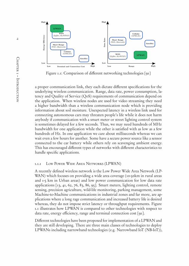
Figure 1.1: Comparison of different networking technologies [91]
a proper communication link, they each dictate different specifications for theunderlying wireless communication. Range, data rate, power consumption, la-tency and Quality of Service (QoS) requirements of communication depend onthe application. When wireless nodes are used for video streaming they needa higher bandwidth than a wireless communication node which is providinginformation about soil moisture. Unexpected latency in a wireless link used forconnecting autonomous cars may threaten people’s life while it does not harmanybody if communication with a smart meter or street lighting control systemis sometimes delayed for a few seconds. Thus, we may need hundreds of MHzbandwidth for one application while the other is satisfied with as low as a fewhundreds of Hz. In one application we care about milliseconds whereas we canwait even a few hours for another. Some have a secure power source like a sensorconnected to the car battery while others rely on scavenging ambient energy.This has encouraged different types of networks with different characteristics tohandle specific applications.
1.1.1 Low Power Wide Area Networks (LPWAN)
A recently defined wireless network is the Low Power Wide Area Network (LP-WAN) which focuses on providing a wide area coverage (10-50km in rural areasand 1-5 km in Urban areas) and low power communication for low data rateapplications [13, 41, 62, 76, 83, 86, 95]. Smart meters, lighting control, remotesensing, precision agriculture, wild-life monitoring, parking management, someMachine-to-Machine communications in industrial zones and far more, are ap-plications where a long rage communication and increased battery life is desiredwhereas, they do not impose strict latency or throughput requirements. Figure1.1 illustrates how LPWAN is compared to other technologies with respect todata rate, energy efficiency, range and terminal connection cost [91].
Different technologies have been proposed for implementation of a LPWAN andthey are still developing. There are three main classes of technologies to deployLPWANs including narrowband technologies (e.g. Narrowband IoT (NB-IoT)),
550999-L-bw-Siavash550999-L-bw-Siavash550999-L-bw-Siavash550999-L-bw-SiavashProcessed on: 23-11-2020Processed on: 23-11-2020Processed on: 23-11-2020Processed on: 23-11-2020 PDF page: 25PDF page: 25PDF page: 25PDF page: 25
3
1.1.2–Ultra-Narrowband(UNB)Communication
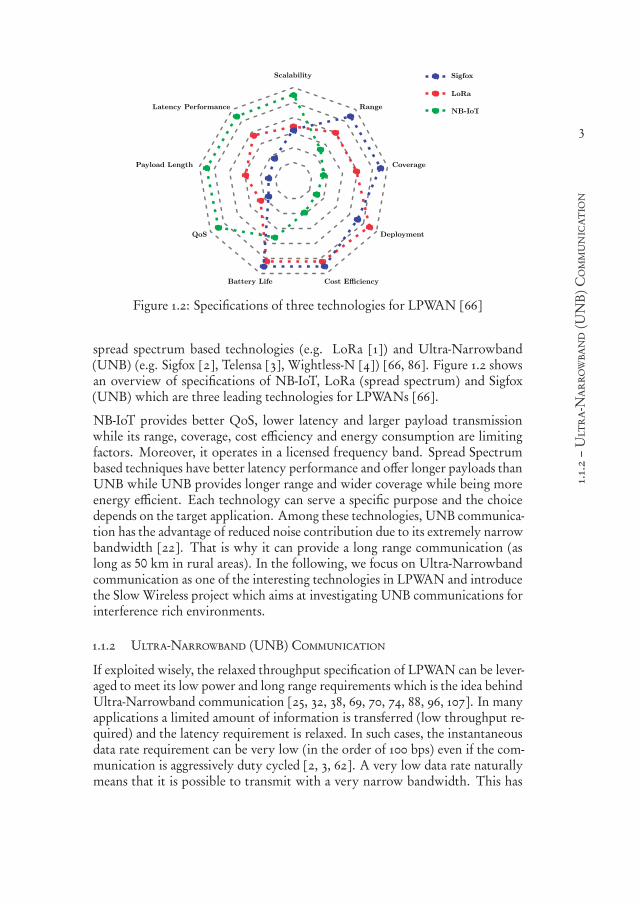
Figure 1.2: Specifications of three technologies for LPWAN [66]
spread spectrum based technologies (e.g. LoRa [1]) and Ultra-Narrowband(UNB) (e.g. Sigfox [2], Telensa [3], Wightless-N [4]) [66, 86]. Figure 1.2 showsan overview of specifications of NB-IoT, LoRa (spread spectrum) and Sigfox(UNB) which are three leading technologies for LPWANs [66].
NB-IoT provides better QoS, lower latency and larger payload transmissionwhile its range, coverage, cost efficiency and energy consumption are limitingfactors. Moreover, it operates in a licensed frequency band. Spread Spectrumbased techniques have better latency performance and offer longer payloads thanUNB while UNB provides longer range and wider coverage while being moreenergy efficient. Each technology can serve a specific purpose and the choicedepends on the target application. Among these technologies, UNB communica-tion has the advantage of reduced noise contribution due to its extremely narrowbandwidth [22]. That is why it can provide a long range communication (aslong as 50 km in rural areas). In the following, we focus on Ultra-Narrowbandcommunication as one of the interesting technologies in LPWAN and introducethe Slow Wireless project which aims at investigating UNB communications forinterference rich environments.
1.1.2 Ultra-Narrowband (UNB) Communication
If exploited wisely, the relaxed throughput specification of LPWAN can be lever-aged to meet its low power and long range requirements which is the idea behindUltra-Narrowband communication [25, 32, 38, 69, 70, 74, 88, 96, 107]. In manyapplications a limited amount of information is transferred (low throughput re-quired) and the latency requirement is relaxed. In such cases, the instantaneousdata rate requirement can be very low (in the order of 100 bps) even if the com-munication is aggressively duty cycled [2, 3, 62]. A very low data rate naturallymeans that it is possible to transmit with a very narrow bandwidth. This has

550999-L-bw-Siavash550999-L-bw-Siavash550999-L-bw-Siavash550999-L-bw-SiavashProcessed on: 23-11-2020Processed on: 23-11-2020Processed on: 23-11-2020Processed on: 23-11-2020 PDF page: 26PDF page: 26PDF page: 26PDF page: 26
4
Chapter1–
Introduction
encouraged applying Ultra-Narrowband communication which can be benefi-cial in scenarios with a large link budget such as long range communication andinterference-rich environments [62, 74].
In LPWAN technologies a communication system using narrowband single car-rier communication without spread spectrum techniques with a bandwidth inthe order of a few hundreds of Hz is referred to as UNB communication [62, 66].There are different UNB communication technologies used for LPWAN such asTelensa [3], Wieghtless [4] and Sigfox [2].
One of the examples of a commercial UNB-based LPWAN is Sigfox [2]. Witha data rate of 100 bps, it uses a channel of 192 kHz in the Sub-GHz ISM bandand uses Phase-Shift-Keying and Frequency-Shift-Keying modulation schemes.PSK and FSK are the most common modulation techniques in UNB communi-cation technologies [66, 86]. Similar to many other LPWANs, Sigfox uses a startopology where nodes can communicate with a base station and communicationis supported for both uplink and downlink (depending on the node model andtype of network). A base station supports several nodes (up to 50 k devices percell). The communication is performed in short packets (around 200 symbols)during packet times which are on average 2 s [2, 66, 83].
Inspired by the emerging application of UNB communication, the SlowWirelessproject began to investigate the physical layer (PHY) aspects of UNB communi-cations in the ISM band. The project is briefly described in the next section.
1.1.3 The Slow Wireless Project
The ISM band is a popular band for many wireless applications as it is free ofcharge. This makes the interference level very high and requires applications toovercome these high levels. The main idea of the Slow Wireless project is usingUNB communication in an interference rich environment for low throughputnetworks. One of the possible applications is for the nodes which want to op-erate in the 2.4 GHz ISM band which is the same band used by WiFi signals.Considering the large number of devices using WiFi for communications includ-ing smart phones and laptops, it would be challenging for low power nodes tocombat this high level of interference. Moreover, it has been shown that ultra-narrowband is a suitable option for energy scavenging low throughput WSNswhen high levels of interference are experienced from co-existing communica-tion systems. Particularly, when the interference is wideband compared to UNB(such as WiFi in 2.4 GHz band) [63]. Nevertheless, a long range can also beachieved using the same UNB communication, particularly, if it works in thesub-GHz ISM band [63].
The Slow Wireless project focuses on the PHY aspects to investigate UNB com-munications in the ISM band. As one of the work packages in the Slow Wire-less project, the current thesis aims at digital signal processing techniques forlow power and low cost nodes in UNB communications. The UNB nodes are

550999-L-bw-Siavash550999-L-bw-Siavash550999-L-bw-Siavash550999-L-bw-SiavashProcessed on: 23-11-2020Processed on: 23-11-2020Processed on: 23-11-2020Processed on: 23-11-2020 PDF page: 27PDF page: 27PDF page: 27PDF page: 27
5
1.2–UNBChallenges
power constrained in applications where either the node is battery powered oruses energy scavenging techniques. Unlike other communication schemes suchas Orthogonal Frequency Division Multiplexing (OFDM), narrowband com-munication does not require a complicated demodulator and signal processing.Furthermore, low data rate communication does not require a high samplingfrequency which relaxes the requirements for processing resources in the digitalcircuitry. Although low data rate communication relaxes power and computa-tional load on the digital processing part of the node’s receiver, it faces two otherchallenges; frequency offset and temporal fading. These two challenges, as wellas interesting directions to find a solution for them are explained in the nextsection.
1.2 UNB Challenges
1.2.1 Frequency Offset
One of thewell-known challenges inwireless communications is frequency offset.Frequency offset may be a consequence of mismatch between local oscillators inthe transmitter and the receiver or the Doppler shift due to relative movement ofthe receiver and the transmitter. For medium or high data rate communication,it is easier to tolerate frequency offset. For example, the Bluetooth specificationallows an initial frequency offset up to ±75 kHz which is around ±30 ppmfor the carrier frequency of 2.4 GHz [47]. Considering that the data rate inBluetooth is about 1 Mbps, this range of frequency offset is ±7.5% of the datarate.
When the ratio of the data rate (signal bandwidth) to the carrier frequencydecreases, the problem of frequency offset becomes more challenging. In theuplink communication of a UNB network, the base station has enough resourcesto afford precise frequency generation. However, the receiver in the downlinkcommunication is a low power and cheap node which makes precise frequencygeneration far more challenging. In a UNB communication system with a datarate of 100 bps, achieving a frequency precision of about ±7.5% of the data raterequires a precision of less than 9 ppb (parts per billion) in the 868 MHz bandand about 3 ppb in the 2.4 GHz band. Even high precision crystals with 0.2− 2ppm [81] stability lead to a frequency offset between 174−1740 Hz in 868 MHzband which can reach up to more than 17 times the data rate. Such crystals forhigh precision frequency generation are costly and power hungry which is notsuitable for cheap devices and large deployment [38].
The low cost off-the-shelf crystals have an instability in the order of 20 ppm [55].For a UNB communication system working in the 868 MHz band, such a preci-sion causes a frequency offset around ±17 kHz which is 170 times the data rate.Thus, for UNB communication, frequency uncertainty is a paramount challenge.In Sigfox, this effect is alleviated using Random Frequency and Time MultipleAccess in the Medium Access Control (MAC) layer. For uplink transmission,

550999-L-bw-Siavash550999-L-bw-Siavash550999-L-bw-Siavash550999-L-bw-SiavashProcessed on: 23-11-2020Processed on: 23-11-2020Processed on: 23-11-2020Processed on: 23-11-2020 PDF page: 28PDF page: 28PDF page: 28PDF page: 28
6
Chapter1–
Introduction
each node transmits a signal at a random time instant and frequency (includedin the 192 kHz band). The base station scans the whole band (192 kHz) anddetects uplink messages. Then, for a downlink message, the base station extractsthe exact carrier frequency of the received signal from each node and transmitsexactly on the same frequency. The effect of such a MAC layer on interferenceand network performance have been discussed extensively in [37, 38].
Although the frequency offset problem can be partially addressed in the MAClayer (similar to what is done for Sigfox), due to the frequency drift caused by thelow cost crystals as well as long turnaround times (30 s), the frequency offset canstill become a few times the signal bandwidth [55]. Moreover, such a solutionlimits the downlink transmission to the reception of an uplink message. In otherwords, the base station can only talk to a node a short time after the receptionof an uplink message. If the receiver node can tolerate a large frequency offset,not only low cost and low power crystals can be easily used but also the strictcriterion on downlink communication in UNB networks can be relaxed.
1.2.2 Scalable Offset Tolerance
Generally speaking, in a wireless receiver, the frequency offset should be esti-mated and compensated in order for the demodulator and detector to performcorrectly. To handle a large frequency offset in the receivers, there are usuallytwo or more steps of frequency synchronization. First, a coarse estimation ofthe frequency offset is achieved and the frequency offset is compensated [68].Compensation at this step might be done in the digital domain or in the analogdomain by tuning the local frequency synthesizer. When the frequency offsetis decreased to a fraction of the data rate, the residual frequency offset can beestimated and compensated before demodulation and detection.
The process of carrier synchronization is power hungry and costly. Therefore,offset tolerant demodulators have been proposed as an alternative to this conven-tional method of estimating and compensating frequency offset [14, 18, 19, 43,49, 50, 55, 56, 75, 84, 94, 99, 102, 106]. These demodulators have been designedfor both Phase Shift Keying (PSK) and Frequency Shift Keying (FSK) modu-lations. Various offset tolerant demodulators for FSK have been proposed forBluetooth receivers as well as Wireless Sensor Networks (WSN) applications[14, 18, 43, 56, 102]. A class of demodulators based on Double Differential PSK(DDPSK) have also been proposed which are capable of tolerating frequencyoffset [49, 84, 94, 99, 106]. In most of these proposed methods, the allowed offsettolerance is limited and it is assumed that the frequency offset is compensatedso that it is brought in the range of the data rate using a coarse carrier syn-chronization. Afterwards, using an offset tolerant demodulator, the fine carriersynchronization is avoided to eliminate precise synchronization algorithms. Asexplained in the previous section, for UNB communication, even a frequencyoffset as large as the data rate is significantly small. Thus, it would be interesting
550999-L-bw-Siavash550999-L-bw-Siavash550999-L-bw-Siavash550999-L-bw-SiavashProcessed on: 23-11-2020Processed on: 23-11-2020Processed on: 23-11-2020Processed on: 23-11-2020 PDF page: 29PDF page: 29PDF page: 29PDF page: 29
7
1.2.3–TemporalFadingandOffsetTolerantDemodulators
to apply demodulation schemes with a scalable offset tolerance capability. Inthis way, we can remove (or simplify) the coarse carrier synchronization as well.
Among the proposed demodulators, there are two general architectures that havepotential for high scalability [39, 44, 94, 106]. The main idea of these demod-ulators is using the Discrete Fourier Transform (DFT) for FSK demodulation[39, 44] and Double Differential detection for PSK demodulation [106]. Thesedigital demodulators have been originally designed for low data rate satellite com-munications where the frequency offset caused by Doppler shift can be muchlarger than the data rate [44, 106]. These demodulators can theoretically tolerateany frequency offset as far as the signal is still captured by the input filter. Al-though these demodulators are in principle scalable, they face limitations whenit comes to very large frequency offset (like 1.7− 17 kHz for a 100 bps data ratewhich was mentioned earlier). Nevertheless, these structures can be modified todesign offset tolerant demodulators for UNB communications.
1.2.3 Temporal Fading and Offset Tolerant Demodulators
In addition to frequency offset, temporal fading should be considered in UNBcommunication as well. As shown in [71], for low data rate communication atime-varying channel may cause an error floor. This error floor is more drasticin ultra-narrowband systems due to a longer symbol time. As a consequence oftime-varying behavior, channel estimation at the beginning of a packet is notreliable. Furthermore, using multiple pilot sequences for channel estimationimposes prohibitive overhead due to short packets used in these systems (asshort as 200 symbols [38]). Offset tolerant demodulators proposed for FSKand PSK do not need channel estimation to overcome the phase offset resultingfrom a fading channel. Nevertheless, the attenuation of the signal in presence offading as well as random frequency modulation caused by a frequency-dispersivechannel degrades the performance terribly and may lead to an error floor.
In such circumstances diversity techniques can be utilized to improve perfor-mance [71]. Space diversity is dismissed for wireless sensor nodes because of lowpower and area constraints of the receiver. In a time-varying channel, time diver-sity (using channel coding and interleaving) is a possible solution. Additionally,frequency diversity (using frequency hopping) can be utilized. Both solutions in-volve transmission of redundant information via channel coding. This increaseseither the bit rate or packet time. To keep the packet time constant (avoidinglonger on-time for the RF front-end) while keeping the symbol rate low, higherorder modulation can be used and the offset tolerant demodulators can be ap-plied.
For a PSK modulation, the downside of the increased modulation order is a lossin BER performance. On the other hand, increasing the FSK order increases therequired bandwidth. To achieve a better power and bandwidth trade-off in higherorder modulation, hybrid frequency/phase modulation has been suggested [17,34, 35, 52, 57, 87]. Despite all research performed on different aspects of such a
550999-L-bw-Siavash550999-L-bw-Siavash550999-L-bw-Siavash550999-L-bw-SiavashProcessed on: 23-11-2020Processed on: 23-11-2020Processed on: 23-11-2020Processed on: 23-11-2020 PDF page: 30PDF page: 30PDF page: 30PDF page: 30
8
Chapter1–
Introduction
hybridmodulation, an offset tolerant demodulator, which is capable of toleratingfrequency offset larger than the symbol rate, has not been introduced. If anoffset tolerant demodulator is designed for hybrid modulation, it can increasethe raw bit-rate. Then, this additional raw bit-rate can be used to implementa low complexity diversity technique and improve the performance of UNBcommunication in a time-varying fading channel.
1.3 Research Objectives
So far, offset tolerant demodulators have been introduced as a method which hasproven useful to overcome the challenge of frequency offset. In many applica-tions the offset tolerant demodulators are used to remove the requirement of thefine tune offset tolerance. In UNB communication this fine-tuned frequency off-set, which is a fraction of the signal bandwidth, can be in the order of 10−20 Hzfor a 868 MHz/2.4 GHz carrier. This means that it already needs considerablecoarse carrier recovery before the fine tuning stage.
As mentioned earlier, some protocols like Sigfox, try to solve the offset problemat a higher layer. However, it still imposes limitations on the communicationand, when low cost and low power crystals are used, it still leads to frequencyoffset larger than the signal bandwidth [55]. Considering these facts, an offsettolerant demodulator which is able to tolerate arbitrarily large frequency offsetcan overcome the offset problem and add to the flexibility of the design ofUNB systems and networks. It eliminates the need for costly precise crystalor power hungry thermal compensation and removes carrier recovery loops orconsiderably relaxes their requirements.
The techniques proposed in this work focus on the baseband digital process-ing and are independent of the analog design. Therefore, these techniques areapplicable to different receiver architectures. As an example, a low-IF receiver,which is a popular structure for low power wireless receivers, is shown in Fig-ure 1.3 [55, 64]. The signal frequency is down-converted to a low IntermediateFrequency (IF) (1− 5 MHz), converted to digital samples using an Analog toDigital Converter (ADC) and sent to the digital domain. The down-conversionto baseband, filtering and decimation and, finally, demodulation and detectionare performed in the digital domain. In UNB communications, the signal band-width is very small compared to the IF frequency (in the order of 10−4 of IF) sothe analog section e.g. the analog low-pass filter before the ADC will not have asignificant effect on the demodulator offset tolerance.
Therefore, a digital offset tolerant demodulator that can work independent of theRF front-end can provide flexibility and move the problem and its solution tothe digital domain which can be more power efficient. Besides, the narrowbandfilters required to deal with the UNB signal can be implemented more efficientlyin the digital domain. To achieve a digital demodulator while removing precisecarrier recovery in UNB communications, this thesis focuses on demodulators

550999-L-bw-Siavash550999-L-bw-Siavash550999-L-bw-Siavash550999-L-bw-SiavashProcessed on: 23-11-2020Processed on: 23-11-2020Processed on: 23-11-2020Processed on: 23-11-2020 PDF page: 31PDF page: 31PDF page: 31PDF page: 31
9
1.3–ResearchObjectives
Figure 1.3: A low-IF receiver architecture for wireless communications
which can achieve scalable offset tolerance. Alleviating the frequency offsetchallenge within the PHY layer offers flexibility to higher layers and networkdesigners. In addition to the frequency offset, the temporal fading and usingdiversity as a solution should be investigated. Taking all aforementioned intoaccount, the main research questions can be formulated as follows.
1. What are the limitations of offset tolerant demodulators, which can toleratelarge frequency offset, for UNB communications?
To answer this question a frequency offset tolerant demodulator for FSK isintroduced inspired by an existing DFT-based demodulator. An offset tolerantdemodulator for PSK is also considered. The two demodulators are simulatedfor different offset tolerance ranges and limitations of these demodulators forscalable offset tolerance are investigated.
2. How can the limitations of the demodulators to achieve scalable offset-tolerance be circumvented?
When the limitations of demodulators for FSK and PSK are known, we needto resolve them. It will be shown that the limitation for the offset tolerant PSKdemodulator is Bit Error Rate (BER) performance degradation as a result ofthe increased noise bandwidth. In case of the DFT-based demodulator for FSK,the complexity will be prohibitive when a large offset tolerance is required. Toovercome these challenges, two different algorithms are proposed for PSK andFSK offset tolerant demodulators.
3. How can the temporal fading in UNB communication be counteracted andthe required redundancy for diversity be achieved while using offset tolerantdemodulators?
To combat the fading effect in a time-varying channel, time diversity might beused and it is a particularly interesting solution as it does not add any overheadunlike frequency hopping. Nevertheless, to achieve redundancy used for codingwe need to increase the raw bit-rate. As mentioned earlier, a hybrid frequen-cy/phase modulation can accomplish this task in a more power efficient mannerthan higher order PSK and more bandwidth efficient way than higher orderFSK. Thus, an offset tolerant demodulator for hybrid FSK/PSK modulation isproposed and its performance in a time-varying channel and using time diversityis evaluated.

550999-L-bw-Siavash550999-L-bw-Siavash550999-L-bw-Siavash550999-L-bw-SiavashProcessed on: 23-11-2020Processed on: 23-11-2020Processed on: 23-11-2020Processed on: 23-11-2020 PDF page: 32PDF page: 32PDF page: 32PDF page: 32
10
Chapter1–
Introduction
1.4 Outline
In the next chapter, an overview of FSK and PSK demodulation and their de-modulators is presented. Chapter 3 which is based on [S:3] includes the answerto the first question. A DFT-based demodulator for FSK is introduced and iscompared with an offset tolerant demodulator for PSK. This chapter elaborateson how they perform in the presence of a large frequency offset and what thelimitations of each method are. Then, the next two chapters are dedicated tofinding a solution to address the limitations observed in Chapter 3 and answerthe second question. To address the BER performance loss of a PSK offset toler-ant demodulator in the presence of a large frequency offset, a shifted correlationdemodulator is proposed in Chapter 4 which is based on [S:4]. In Chapter 5,a low complexity synchronization algorithm for the DFT-based demodulatorand its implementation are presented to relax the complexity bottleneck of theFSK offset tolerant demodulator [S:2, 6]. In the next step, Chapter 6 focuseson the third question. Based on [S:1, 5], this chapter presents an offset tolerantdemodulator for hybrid frequency/phase modulation. The demodulator is usedfor incorporating time diversity in a time-varying channel and its performanceis evaluated for different scenarios. Finally, in Chapter 7 conclusions are drawnand recommendations for future work are presented.

550999-L-bw-Siavash550999-L-bw-Siavash550999-L-bw-Siavash550999-L-bw-SiavashProcessed on: 23-11-2020Processed on: 23-11-2020Processed on: 23-11-2020Processed on: 23-11-2020 PDF page: 33PDF page: 33PDF page: 33PDF page: 33
11

550999-L-bw-Siavash550999-L-bw-Siavash550999-L-bw-Siavash550999-L-bw-SiavashProcessed on: 23-11-2020Processed on: 23-11-2020Processed on: 23-11-2020Processed on: 23-11-2020 PDF page: 34PDF page: 34PDF page: 34PDF page: 34
12
550999-L-bw-Siavash550999-L-bw-Siavash550999-L-bw-Siavash550999-L-bw-SiavashProcessed on: 23-11-2020Processed on: 23-11-2020Processed on: 23-11-2020Processed on: 23-11-2020 PDF page: 35PDF page: 35PDF page: 35PDF page: 35
132Background
Before continuing our path to offset tolerant demodulators for UNB commu-nication we need to first have a brief review on the concepts used in the thesisand the conventional modulation and demodulation schemes. The focus of ourwork is on demodulating the received signals in the presence of a frequency off-set; therefore, we mainly discuss the receiver of a wireless communication link.Besides, as mentioned in the previous chapter, the reception of the uplink signalin UNB communication is less challenging as the base station (gateway) doesnot have critical energy restrictions. Thus, the main focus is on the receiverdesign for the downlink communication. In this chapter, first a simple model ofthe wireless receiver and the complex notation of signals are presented. Then,the modulation schemes together with their demodulators are presented. After-wards, the problem of frequency offset is explained and the concept of a receiverwith an offset tolerant demodulator is demonstrated.
In the next section, the system model and signal notations are defined. Sections2.2, 2.3 and 2.4 introduce FSK, PSK and FPSK modulations and some of theirtypical demodulators. Finally, section 2.5 elaborates on the frequency offsetproblem and shows how it is solved in a conventional way and how we are goingto address it in this work.
2.1 System Model and Complex Notations
A wireless signal is transmitted using a sinusoidal carrier with a frequency equalto fc . When information bits are transmitted modulating the frequency or phase,the general form of the transmitted signal during the n t h symbol is as follows.
s(t ) =Ac cos(ωc t +θ(t )), (n− 1)T ≤ t ≤ nT (2.1)
where Ac is the signal amplitude, T is the symbol period, ωc = 2π fc is thecarrier frequency and θ(t ) is the phase of the signal which reflects modulatedinformation either on frequency or phase. In (2.1) a rectangular pulse shape is
550999-L-bw-Siavash550999-L-bw-Siavash550999-L-bw-Siavash550999-L-bw-SiavashProcessed on: 23-11-2020Processed on: 23-11-2020Processed on: 23-11-2020Processed on: 23-11-2020 PDF page: 36PDF page: 36PDF page: 36PDF page: 36
14
Chapter2–Background
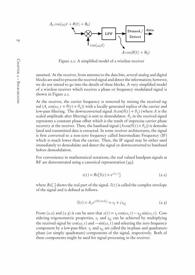
Figure 2.1: A simplified model of a wireless receiver
assumed. At the receiver, from antenna to the data bits, several analog and digitalblocks are used to process the received signal and detect the information; however,we do not intend to go into the details of these blocks. A very simplified modelof a wireless receiver which receives a phase or frequency modulated signal isshown in Figure 2.1.
At the receiver, the carrier frequency is removed by mixing the received sig-nal (Ac cos(ωc t +θ(t )+θ0)) with a locally generated replica of the carrier andlow-pass filtering. The downconverted signal Acos(θ(t ) + θ0) (where A is thescaled amplitude after filtering) is sent to demodulator. θ0 in the received signalrepresents a constant phase offset which is the result of imprecise carrier phaserecovery at the receiver. Then, the baseband signal (Acos(θ(t )+θ0)) is demodu-lated and transmitted data is extracted. In some receiver architectures, the signalis first converted to a non-zero frequency called Intermediate Frequency (IF)which is much lower than the carrier. Then, the IF signal may be either usedimmediately to demodulate and detect the signal or downconverted to basebandbefore demodulation.
For convenience in mathematical notations, the real valued bandpass signals atRF are demonstrated using a canonical representation [45]:
s(t ) = Re[ s(t )× e jωc t ] (2.2)
where Re[.] shows the real part of the signal. s(t ) is called the complex envelopeof the signal and is defined as follows.
s(t ) =Ac e j (θ(t )+θ0) = sI + j sQ (2.3)
From (2.2) and (2.3) it can be seen that s(t ) = sI cos(ωc t )− sQ sin(ωc t ). Con-sidering trigonometric properties, sI and sQ can be achieved by multiplyingthe received signal by cos(ωc t ) and − sin(ωc t ) and selecting the zero frequencycomponent by a low-pass filter. sI and sQ are called the in-phase and quadrature-phase (or simply quadrature) components of the signal, respectively. Both ofthese components might be used for signal processing in the receiver.

550999-L-bw-Siavash550999-L-bw-Siavash550999-L-bw-Siavash550999-L-bw-SiavashProcessed on: 23-11-2020Processed on: 23-11-2020Processed on: 23-11-2020Processed on: 23-11-2020 PDF page: 37PDF page: 37PDF page: 37PDF page: 37
15
2.2–FSKModulation
Using the complex envelope notation and assuming an Additive White GaussianNoise (AWGN) channel, the received baseband signal is:
r (t ) =Ac e j (θ(t )+θ0)+ n(t ) (2.4)
where r (t ) is the baseband signal and n(t ) is complex Gaussian noise (n(t ) isnot shown in Figure 2.1). In most practical cases, the exact phase recovery of thecarrier is cumbersome. That is why such a phase offset is considered and demod-ulators are designed to perform independent of phase offset. The demodulatorswhich do not rely on carrier phase recovery for correct performance are callednon-coherent demodulators.
2.2 FSK Modulation
FSK modulation transmits information by changing the frequency of the trans-mitted carrier. For Binary FSK (BFSK) the complex envelope of the modulatedsignal during the n t h symbol period is as follows.
s(t ) =Ac e j bnhπT t , (n− 1)T ≤ t ≤ nT (2.5)
where bn =−1,+1 is the transmitted symbol and T is the symbol period. h iscalled modulation index which determines the separation between two possibletones of a BFSK signal which is called frequency separation defined as ωs e p =2πh/T .
A more practical version of an FSK signal is called Continuous Phase FSK(CPFSK). The phase of a continuous phase binary FSK is derived as follows[103].
θ(t ) =πhT
bn(t − (n− 1)T )+πhn−2∑
i=0
bi , (n− 1)T ≤ t ≤ nT (2.6)
Using CPFSK, the received signal during the n t h symbol is as follows.
r (t ) =Ac e j (θ(t )+θ0)+ n(t ), (n− 1)T ≤ t < nT (2.7)
where θ(t ) is obtained from (2.6), θ0 is a constant phase offset and n(t ) repre-sents complex Gaussian noise. The FSK modulated signal can be demodulatedand detected using a non-coherent demodulator for orthogonal modulations asshown in Figure 2.2 [45].
In each branch, the signal is multiplied by the conjugate of one of the possibletransmitted frequencies and, then, integrated over a symbol period. Afterwards,
550999-L-bw-Siavash550999-L-bw-Siavash550999-L-bw-Siavash550999-L-bw-SiavashProcessed on: 23-11-2020Processed on: 23-11-2020Processed on: 23-11-2020Processed on: 23-11-2020 PDF page: 38PDF page: 38PDF page: 38PDF page: 38
16
Chapter2–Background
Figure 2.2: Non-coherent demodulator for BFSK based on correlation
Figure 2.3: Cross Differentiate Multiply demodulator for BFSK
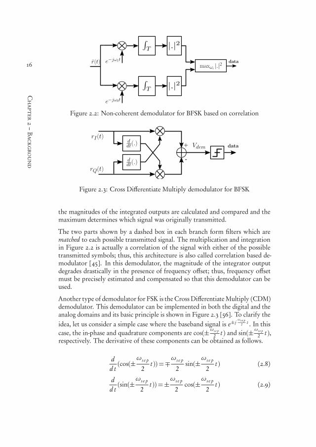
the magnitudes of the integrated outputs are calculated and compared and themaximum determines which signal was originally transmitted.
The two parts shown by a dashed box in each branch form filters which arematched to each possible transmitted signal. The multiplication and integrationin Figure 2.2 is actually a correlation of the signal with either of the possibletransmitted symbols; thus, this architecture is also called correlation based de-modulator [45]. In this demodulator, the magnitude of the integrator outputdegrades drastically in the presence of frequency offset; thus, frequency offsetmust be precisely estimated and compensated so that this demodulator can beused.
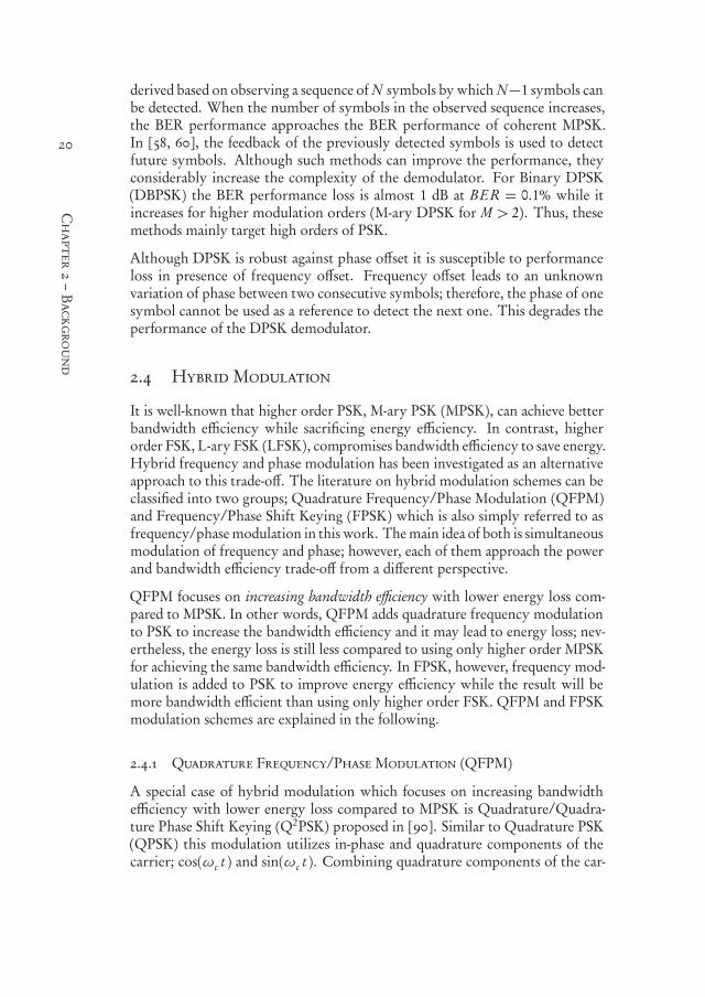
Another type of demodulator for FSK is the Cross DifferentiateMultiply (CDM)demodulator. This demodulator can be implemented in both the digital and theanalog domains and its basic principle is shown in Figure 2.3 [56]. To clarify theidea, let us consider a simple case where the baseband signal is e± j
ωs e p2 t . In this
case, the in-phase and quadrature components are cos(±ωs e p
2 t ) and sin(±ωs e p
2 t ),respectively. The derivative of these components can be obtained as follows.
dd t(cos(±
ωs e p
2t )) =∓
ωs e p
2sin(±
ωs e p
2t ) (2.8)
dd t(sin(±
ωs e p
2t )) =±
ωs e p
2cos(±
ωs e p
2t ) (2.9)

550999-L-bw-Siavash550999-L-bw-Siavash550999-L-bw-Siavash550999-L-bw-SiavashProcessed on: 23-11-2020Processed on: 23-11-2020Processed on: 23-11-2020Processed on: 23-11-2020 PDF page: 39PDF page: 39PDF page: 39PDF page: 39
17
2.2–FSKModulation
Figure 2.4: FSK demodulator based on converting frequency modulated signalto squarewave (e.g. using limiter)
Thus, the result of multiplications in the upper and the lower branch shown byVI and VQ , respectively, are as follows.
VI =±ωs e p
2cos2(±
ωs e p
2t ) (2.10)
VQ =∓ωs e p
2sin2(±
ωs e p
22t ) (2.11)
Finally, subtracting VQ from VI , the output before the decision block is asfollows.
Vd e m =±ωs e p
2[cos2(±
ωs e p
2t )+ sin2(±
ωs e p
2t )] (2.12)
Since the sum of the terms in paranthesis is always equal to one, the sign of Vd e monly depends on the sign of modulated frequency. It is clear that the outputof such a demodulator will be affected by a non-zero frequency offset and thetransmitted data cannot be retrieved correctly.
Another class of FSK demodulators is based on generating a square wave fromthe received frequency modulated signal and calculating the frequency accordingto transitions [43, 102, 105]. A general block diagram for this type of demod-ulators is shown in Figure 2.4. The square wave might be generated using alimiter which amplifies the input sinusoidal signal to saturation level or applyingphase to digital converter methods such as phase quantization [43]. In a digitalimplementation the zero-crossings of this square wave can be counted and thefrequency (and thus the transmitted data) is detected based on the number ofcrossing per symbol period (called a zero-crossing demodulator).
Alternatively, the square wave can be sent to a pulse generator to generate equalwidth pulses at each edge. Since the density of these equal width pulses changeswith frequency, averaging them using a low-pass filter can convert the frequencyinformation to a variable voltage which will be used for data detection. In thistype of demodulators, frequency offset changes the intensity of zero-crossingsfrom the expected values and adds a DC-level to the output of the demodulatorsand degrades detection performance.

550999-L-bw-Siavash550999-L-bw-Siavash550999-L-bw-Siavash550999-L-bw-SiavashProcessed on: 23-11-2020Processed on: 23-11-2020Processed on: 23-11-2020Processed on: 23-11-2020 PDF page: 40PDF page: 40PDF page: 40PDF page: 40
18
Chapter2–Background
In some FSK demodulators, a delayed or phase shifted version of input IF (Inter-mediate Frequency) signal is generated and used for demodulation [14, 19, 50, 92].FSK demodulation using a Delay Locked Loop (DLL) is an example of this typeof demodulators. After converting IF FSK signal to a square wave, it is sampledby a delayed version of itself with a delay, generated by a DLL exactly equal tothe period of the IF frequency. Depending on whether the received signal hasa higher or lower frequency than the expected IF frequency, the rising edges ofthe delayed version lags or leads the rising edges of the signal itself. This char-acteristic is used to detect the data sequence [14]. In a DLL based demodulator,frequency offset means that the generated delay is no longer equal to the periodof the IF input signal which destroys performance of the demodulator [19].
As mentioned above, the BER performance of all of these demodulators degradesin the presence of frequency offset. None of the above demodulators are offsettolerant in nature and they either need a frequency controller or some additionaltechniques to improve their robustness against frequency offset.
2.3 PSK Modulation
Phase Shift Keying (PSK) is a digital modulation technique which transmitsinformation by changing the phase of the transmitted signal. The complexenvelope of an M-ary PSK signal is:
s(t ) =∑
ng (t − nT )e j (ϕn+θ0), (2.13)
where ϕn =2πiM ( i = 0, ..., M−1) is determined by the transmitted symbol and θ0
is a constant phase offset which is due to imprecise carrier phase recovery. g (t )is the pulse shape used for PSK to limit the bandwidth of the transmitted signalin band-limited scenarios. In this work, a rectangular pulse shape is considered;thus, the received MPSK signal during the n t h symbol period is:
r (t ) =Ac e j (ϕn+θ0)+ n(t ), (n− 1)T ≤ t ≤ nT (2.14)
Detecting each symbol stand-alone requires prior knowledge of θ0 which iscomplex to achieve. To enable non-coherent detection, a variation of PSK mod-ulation is used known as Differential PSK (DPSK).
2.3.1 Differential PSK (DPSK)
For DPSK the phase of each symbol will be used as a reference to determinethe phase of the next symbol. If θ0 is constant during two consecutive symbols,its effect will be removed. To make the detection possible in the receiver, adifferential encoder in the transmitter is used which encodes information in the

550999-L-bw-Siavash550999-L-bw-Siavash550999-L-bw-Siavash550999-L-bw-SiavashProcessed on: 23-11-2020Processed on: 23-11-2020Processed on: 23-11-2020Processed on: 23-11-2020 PDF page: 41PDF page: 41PDF page: 41PDF page: 41
19
2.3.1–DifferentialPSK(DPSK)
Figure 2.5: Differential encoder and DPSK demodulator
difference between the phases of consecutive symbols. The differential encoderand the DPSK demodulator for M-ary PSK modulation are shown in Figure 2.5.
In the transmitter, data is mapped to the symbols of MPSK to generate e jαn .Afterwards, a differential encoder is applied to achieve e jϕn which is the trans-mitted phase. In the demodulator, the signal passes through a Matched Filter(MF) to maximize the Signal to Noise Ratio (SNR). When a rectangular pulseshape is assumed, this filter would be as simple as integration over a symbolperiod. The output of the filter is sampled at the symbol rate and the values aresent to a differential decoder. The differential decoder multiplies the output ofthe integrator for each symbol with the conjugate of integrator output of theprevious symbol. Using the differential decoder and considering a signal modelsimilar to (2.14), the decision variable dn after decoder is:
dn =Ae j∆ϕn + n′ (2.15)
where A= (Ac T )2, ∆ϕn = ϕn − ϕn−1 and n′ represents all noise components.Now, looking into the differential encoder, we can see that αn = ϕn − ϕn−1.Therefore, the transmitted information can be detected based on dn using thefollowing detection criterion for MPSK.
αn = arg maxαi∈A
Re[dn × exp(− jαi )] (2.16)
where A= 2πiM |i = 0, ..., M−1 is the set of possible symbol phases for anMPSK
modulation.
As shown here, to detect a DPSK signal a noisy reference (the phase of theprevious symbol) is used which increases the error probability compared tocoherent detection. A variety of methods have been introduced in literatureto overcome this BER performance loss of DPSK. In [21], a multiple symboldetection method is proposed for DMPSK. In this method a decision variable is
550999-L-bw-Siavash550999-L-bw-Siavash550999-L-bw-Siavash550999-L-bw-SiavashProcessed on: 23-11-2020Processed on: 23-11-2020Processed on: 23-11-2020Processed on: 23-11-2020 PDF page: 42PDF page: 42PDF page: 42PDF page: 42
20
Chapter2–Background
derived based on observing a sequence of N symbols by which N−1 symbols canbe detected. When the number of symbols in the observed sequence increases,the BER performance approaches the BER performance of coherent MPSK.In [58, 60], the feedback of the previously detected symbols is used to detectfuture symbols. Although such methods can improve the performance, theyconsiderably increase the complexity of the demodulator. For Binary DPSK(DBPSK) the BER performance loss is almost 1 dB at BER = 0.1% while itincreases for higher modulation orders (M-ary DPSK for M > 2). Thus, thesemethods mainly target high orders of PSK.
Although DPSK is robust against phase offset it is susceptible to performanceloss in presence of frequency offset. Frequency offset leads to an unknownvariation of phase between two consecutive symbols; therefore, the phase of onesymbol cannot be used as a reference to detect the next one. This degrades theperformance of the DPSK demodulator.
2.4 Hybrid Modulation
It is well-known that higher order PSK, M-ary PSK (MPSK), can achieve betterbandwidth efficiency while sacrificing energy efficiency. In contrast, higherorder FSK, L-ary FSK (LFSK), compromises bandwidth efficiency to save energy.Hybrid frequency and phase modulation has been investigated as an alternativeapproach to this trade-off. The literature on hybrid modulation schemes can beclassified into two groups; Quadrature Frequency/Phase Modulation (QFPM)and Frequency/Phase Shift Keying (FPSK) which is also simply referred to asfrequency/phasemodulation in this work. Themain idea of both is simultaneousmodulation of frequency and phase; however, each of them approach the powerand bandwidth efficiency trade-off from a different perspective.
QFPM focuses on increasing bandwidth efficiency with lower energy loss com-pared to MPSK. In other words, QFPM adds quadrature frequency modulationto PSK to increase the bandwidth efficiency and it may lead to energy loss; nev-ertheless, the energy loss is still less compared to using only higher order MPSKfor achieving the same bandwidth efficiency. In FPSK, however, frequency mod-ulation is added to PSK to improve energy efficiency while the result will bemore bandwidth efficient than using only higher order FSK. QFPM and FPSKmodulation schemes are explained in the following.
2.4.1 Quadrature Frequency/Phase Modulation (QFPM)
A special case of hybrid modulation which focuses on increasing bandwidthefficiency with lower energy loss compared to MPSK is Quadrature/Quadra-ture Phase Shift Keying (Q2PSK) proposed in [90]. Similar to Quadrature PSK(QPSK) this modulation utilizes in-phase and quadrature components of thecarrier; cos(ωc t ) and sin(ωc t ). Combining quadrature components of the car-

550999-L-bw-Siavash550999-L-bw-Siavash550999-L-bw-Siavash550999-L-bw-SiavashProcessed on: 23-11-2020Processed on: 23-11-2020Processed on: 23-11-2020Processed on: 23-11-2020 PDF page: 43PDF page: 43PDF page: 43PDF page: 43
21
2.4.2–Frequency/PhaseShiftKeying(FPSK)
rier with two sinusoidal pulse shapes (cos(πt/2T ) and sin(πt/2T ) where thebit rate is Tb = 2/T ), the following four signals are derived [90].
s1(t ) = cos(πt/2T )cos(ωc t )s2(t ) = sin(πt/2T )cos(ωc t )s3(t ) = cos(πt/2T ) sin(ωc t )s4(t ) = sin(πt/2T ) sin(ωc t ) (2.17)
Binary data (−1 or +1) is transmitted with each signal and the sum of thesefour can generate 16 different symbols. Q2PSK is twice as bandwidth efficientas QPSK while a coherent optimum receiver for Q2PSK can perform similar toQPSK [90]. To provide the same bandwidth efficiency with higher order PSK,a 16PSK modulation must be used which needs around 7 dB larger Eb/N0 thanQ2PSK at BER= 0.1%.
For a more practical scenario where carrier phase estimation is not feasible,a differentially coherent receiver for Q2PSK is proposed in [27]. Althoughcoherent demodulators of Q2PSK andQPSK have similar BER performance, thenon-coherent demodulator of Q2PSK requires 1 dBmore Eb/N0 than differentialQPSK at BER = 0.1%. Thus, the bandwidth efficiency is achieved and powerefficiency is sacrificed but still the power loss is lower compared to using onlyhigher order PSK.
The concept of using quadrature components of the carrier was further extendedto N frequency tones in [33]. It uses quadrature components of N differentfrequency tones in combination with BPSK resulting in a quadrature frequen-cy/phase modulation with N different frequencies, NQFPM. The differentiallycoherent detection of this generalized quadrature modulation is proposed in [16].One of the problems associated with the quadrature frequency/phase modula-tion is its non-constant envelope which has encouraged researchers to suggestspecial coding techniques to avoid envelope variation at the expense of decreasedbandwidth efficiency [15, 90].
In low data rate applications, highly bandwidth efficient modulation is not theprimary concern; therefore, FPSK modulation which focuses on energy effi-ciency and has a constant envelope is a better choice than QFPM. The nextsubsection explains FPSK modulation.
2.4.2 Frequency/Phase Shift Keying (FPSK)
The main difference between FPSK and QFPM is that both in-phase and quadra-ture components of the carrier are modulated with the same frequency. UsingFPSK decreases bandwidth efficiency but improves BER performance compared

550999-L-bw-Siavash550999-L-bw-Siavash550999-L-bw-Siavash550999-L-bw-SiavashProcessed on: 23-11-2020Processed on: 23-11-2020Processed on: 23-11-2020Processed on: 23-11-2020 PDF page: 44PDF page: 44PDF page: 44PDF page: 44
22
Chapter2–Background
Figure 2.6: A non-coherent demodulator for FPSK.
to QFPM. One of the early examples of FPSK was proposed in [87]. The com-plex envelop of the modulated signal is as follows.
s(t ) =Ac e j (ωn t+ϕn ), (n− 1)T ≤ t < nT (2.18)
whereωn = mnωs e p
2 and mn = 2i−(L+1) (for i = 1, ..., L) determines the indexof the symbol for FSK. ϕn is the modulated phase during the n t h symbol. Todemodulate such a signal, a combination of FSK and PSK demodulators mustbe used.
The non-coherent demodulator for FPSK which is a combination of FSK andDPSK is shown in Figure 2.6 [34]. First, FSK is demodulated using non-coherentdemodulation. Afterwards, the result of FSK detection is used to determinethe correct branch which must be sent to the next stage which is a DPSK de-modulator. Similar to previous demodulators introduced in this chapter, theperformance of the demodulator in Figure 2.6 depends on generating an exactreplica of the carrier frequency at the receiver.
2.5 Frequency Offset; Compensate or Tolerate
The mentioned demodulators need an exact replica of the received carrier fre-quency in the receiver. However, this may not be available at the receiver dueto the mismatch between oscillators in the transmitter and the receiver or theDoppler shift between the transceiver nodes. In the presence of a frequencyoffset, the baseband received signal during the n t h symbol is as follows.
r (t ) =Ac e j (ωO t+θ(t )+θ0)+ n(t ), (n− 1)T ≤ t ≤ nT (2.19)
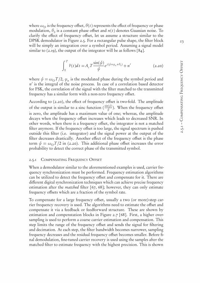
550999-L-bw-Siavash550999-L-bw-Siavash550999-L-bw-Siavash550999-L-bw-SiavashProcessed on: 23-11-2020Processed on: 23-11-2020Processed on: 23-11-2020Processed on: 23-11-2020 PDF page: 45PDF page: 45PDF page: 45PDF page: 45
23
2.5.1–CompensatingFrequencyOffset
whereωO is the frequency offset, θ(t ) represents the effect of frequency or phasemodulation, θ0 is a constant phase offset and n(t ) denotes Guassian noise. Toclarify the effect of frequency offset, let us assume a structure similar to theDPSK demodulator in Figure 2.5. For a rectangular pulse shape, the filter blockwill be simply an integration over a symbol period. Assuming a signal modelsimilar to (2.19), the output of the integrator will be as follows [84].
∫ T
0r (t )d t =Ac T
sin(ψ)ψ
e j (ψ+ϕn+θ0)+ n′ (2.20)
where ψ = ωO T /2, ϕn is the modulated phase during the symbol period andn′ is the integral of the noise process. In case of a correlation based detectorfor FSK, the correlation of the signal with the filter matched to the transmittedfrequency has a similar form with a non-zero frequency offset.
According to (2.20), the effect of frequency offset is two-fold. The amplitudeof the output is similar to a sinc function ( sin(ψ)
ψ ). When the frequency offsetis zero, the amplitude has a maximum value of one; whereas, the amplitudedecays when the frequency offset increases which leads to decreased SNR. Inother words, when there is a frequency offset, the integrator is not a matchedfilter anymore. If the frequency offset is too large, the signal spectrum is pushedoutside this filter (i.e. integrator) and the signal power at the output of thefilter decreases drastically. Another effect of the frequency offset is the phaseterm ψ = ωO T /2 in (2.20). This additional phase offset increases the errorprobability to detect the correct phase of the transmitted symbol.
2.5.1 Compensating Frequency Offset
When a demodulator similar to the aforementioned examples is used, carrier fre-quency synchronization must be performed. Frequency estimation algorithmscan be utilized to detect the frequency offset and compensate for it. There aredifferent digital synchronization techniques which can achieve precise frequencyestimation after the matched filter [67, 68]; however, they can only estimatefrequency offsets which are a fraction of the symbol rate.
To compensate for a large frequency offset, usually a two (or more)-step car-rier frequency recovery is used. The algorithms need to estimate the offset andcompensate it via a feedback or feedforward structure. These are shown byestimation and compenstation blocks in Figure 2.7 [68]. First, a higher over-sampling is used to perform a coarse carrier estimation and compensation. Thisstep limits the range of the frequency offset and sends the signal for filteringand decimation. At each step, the filter bandwidth becomes narrower, samplingfrequency decreases and the residual frequency offset becomes smaller. Before fi-nal demodulation, fine-tuned carrier recovery is used using the samples after thematched filter to estimate frequency with the highest precision. This is shown
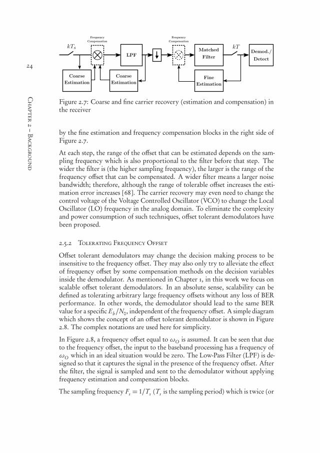
550999-L-bw-Siavash550999-L-bw-Siavash550999-L-bw-Siavash550999-L-bw-SiavashProcessed on: 23-11-2020Processed on: 23-11-2020Processed on: 23-11-2020Processed on: 23-11-2020 PDF page: 46PDF page: 46PDF page: 46PDF page: 46
24
Chapter2–Background
Figure 2.7: Coarse and fine carrier recovery (estimation and compensation) inthe receiver
by the fine estimation and frequency compensation blocks in the right side ofFigure 2.7.
At each step, the range of the offset that can be estimated depends on the sam-pling frequency which is also proportional to the filter before that step. Thewider the filter is (the higher sampling frequency), the larger is the range of thefrequency offset that can be compensated. A wider filter means a larger noisebandwidth; therefore, although the range of tolerable offset increases the esti-mation error increases [68]. The carrier recovery may even need to change thecontrol voltage of the Voltage Controlled Oscillator (VCO) to change the LocalOscillator (LO) frequency in the analog domain. To eliminate the complexityand power consumption of such techniques, offset tolerant demodulators havebeen proposed.
2.5.2 Tolerating Frequency Offset
Offset tolerant demodulators may change the decision making process to beinsensitive to the frequency offset. They may also only try to alleviate the effectof frequency offset by some compensation methods on the decision variablesinside the demodulator. As mentioned in Chapter 1, in this work we focus onscalable offset tolerant demodulators. In an absolute sense, scalability can bedefined as tolerating arbitrary large frequency offsets without any loss of BERperformance. In other words, the demodulator should lead to the same BERvalue for a specific Eb/N0, independent of the frequency offset. A simple diagramwhich shows the concept of an offset tolerant demodulator is shown in Figure2.8. The complex notations are used here for simplicity.
In Figure 2.8, a frequency offset equal to ωO is assumed. It can be seen that dueto the frequency offset, the input to the baseband processing has a frequency ofωO which in an ideal situation would be zero. The Low-Pass Filter (LPF) is de-signed so that it captures the signal in the presence of the frequency offset. Afterthe filter, the signal is sampled and sent to the demodulator without applyingfrequency estimation and compensation blocks.
The sampling frequency Fs = 1/Ts (Ts is the sampling period) which is twice (or

550999-L-bw-Siavash550999-L-bw-Siavash550999-L-bw-Siavash550999-L-bw-SiavashProcessed on: 23-11-2020Processed on: 23-11-2020Processed on: 23-11-2020Processed on: 23-11-2020 PDF page: 47PDF page: 47PDF page: 47PDF page: 47
25
2.5.2–ToleratingFrequencyOffset
Figure 2.8: Simple block diagram of a receiver with offset tolerant demodulator
Figure 2.9: The relation between signal bandwidth (BS ), sampling frequency(Fs ), filter bandwidth (BF ) and maximum tolerable frequency offset ( fO,max )
higher than) the filter bandwidth to avoid noise folding and aliasing. The relationbetween the filter bandwidth, minimum sampling frequency and the tolerablefrequency offset are shown in Figure 2.9. In this figure, BF is the filter bandwidth,Fs is the sampling frequency with complex samples and the signal bandwidth isdenoted by BS . If the demodulator has scalable offset tolerance, the only factorwhich determines the frequency offset will be the filter bandwidth. Focusingon this interpretation of a scalable frequency offset tolerance, the next chapterinvestigates offset tolerant demodulators for ultra-narrowband communicationsand their limitations for scalable offset tolerance.

550999-L-bw-Siavash550999-L-bw-Siavash550999-L-bw-Siavash550999-L-bw-SiavashProcessed on: 23-11-2020Processed on: 23-11-2020Processed on: 23-11-2020Processed on: 23-11-2020 PDF page: 48PDF page: 48PDF page: 48PDF page: 48
26

550999-L-bw-Siavash550999-L-bw-Siavash550999-L-bw-Siavash550999-L-bw-SiavashProcessed on: 23-11-2020Processed on: 23-11-2020Processed on: 23-11-2020Processed on: 23-11-2020 PDF page: 49PDF page: 49PDF page: 49PDF page: 49
273Offset Tolerant Demodulators
for UNB Communications
Abstract – To achieve scalable offset tolerance, this chapter focuses on demod-ulators for FSK and PSKwhich have the potential of tolerating large frequencyoffset. Two offset tolerant demodulators are investigated for FSK and PSK inthe presence of frequency offset which can be several times the symbol rate. ForFSK modulation, an existing DFT-based demodulator is modified consider-ing UNB applications. For PSK, a Double Differential scheme (DDPSK) isintroduced which is a known offset tolerant demodulator. To ensure a faircomparison between these two demodulators, a timing synchronization forDDPSK is designed and used in our simulations. These demodulators are sim-ulated for large frequency offset and their BER performance and complexityare compared. Particularly, the effect of a wide filter required to capture thesignal in the presence of a large frequency offset is considered. The trade-offbetween BER performance and complexity for different filter bandwidths isdiscussed. Both methods work independent of frequency offset, however, it isshown that a wide filter degrades the BER performance of DDBPSK, whereas,the DFT-based demodulator for FSK is not affected by filter bandwidth. Thisrobustness is obtained at the expense of increased computational load. Theresults clarify the limitations of these two demodulators which will be dealtwith in the next chapters.
3.1 Introduction
Offset tolerant demodulators have been proposed to tackle the frequency offsetproblem for both FSK and PSK modulations. Low data rate applications wherea signal experiences a large Doppler shift, such as satellite communications, areapplications of offset tolerant demodulators [39, 44, 106]. Moreover, in some
This chapter is based on [S:3].

550999-L-bw-Siavash550999-L-bw-Siavash550999-L-bw-Siavash550999-L-bw-SiavashProcessed on: 23-11-2020Processed on: 23-11-2020Processed on: 23-11-2020Processed on: 23-11-2020 PDF page: 50PDF page: 50PDF page: 50PDF page: 50
28
Chapter3–OffsetTolerantDemodulatorsforUNBCommunications
other applications like Bluetooth, the receivers are expected to be able to affordfrequency uncertainty. This enables designers to achieve a low cost and lowpower receivers by simplifying frequency generation [47]. In this chapter, theoffset tolerant demodulators are considered for ultra-narrowband communica-tions. As mentioned earlier, our target is to achieve scalable offset tolerance.For this purpose, two offset tolerant demodulators for FSK and PSK, which canpotentially tolerate a relatively large frequency offset (multiple times the sym-bol rate), are investigated. These two demodulators are simulated for differentranges of tolerable frequency offset and their BER performance and complexityare evaluated and compared. This helps us to find out the limitations of thesedemodulators and address them in the next chapters.
For FSK modulated signals, different offset tolerant demodulators have beenproposed. A review on these demodulators (presented in the next section) showsthat a demodulator based on the Discrete Fourier Transform (DFT) [44] has thepotential of achieving scalable offset tolerance. The target of the demodulatorin [44] is to tolerate largely varying Doppler shift which is faced in Low EarthOrbit (LEO) satellite communications. Since UNB communication is mostlyused for fixed nodes, a largely varying Doppler shift is not a concern. Therefore,we introduce a modified version of the DFT-based demodulator here. To enablewindow synchronization when a frequency offset is experienced, a DFT-basedwindow synchronization algorithm is proposed in [44]. For tolerating largefrequency offset using the DFT-based demodulator, it must be implementedtogether with this window synchronization, thus, this algorithm is discussedhere as a phase of the demodulator operation.
For offset tolerant PSK demodulation, the concept of Double Differential encod-ing and an autocorrelation based demodulator (ACD) has been introduced in[94]. It is an extension to the concept of Differential PSK (DPSK) which removesthe phase offset. DDPSK can remove the effect of frequency offset regardlessof its value; therefore, it is used as an offset tolerant PSK demodulator in theanalyses of this chapter. As mentioned above, the DFT-based demodulator uses awindow synchronization algorithm. To ensure a fair complexity comparison forFSK and PSK offset tolerant demodulators, the synchronization of the samplesof a symbol in DDPSK must be considered as well. For this purpose, a simplesynchronization method for DDPSK is introduced and used in this chapter.
In the next step, the modified DFT-based demodulator for FSK and the DDPSKwith the proposed synchronization method are evaluated for different rangesof frequency offset tolerance and their BER performance and complexity areinvestigated. This analysis clarifies the limitations of these two demodulators andpinpoints the challenges that need to be addressed for a scalable offset tolerance.
This chapter is organized as follows. In the next section, a short overview ofoffset tolerant demodulators for FSK is presented followed by an explanation ofthe DFT-based demodulator for FSK and its modified version in section 3.3. Insection 3.4, the DDPSK demodulator and our proposed synchronization scheme

550999-L-bw-Siavash550999-L-bw-Siavash550999-L-bw-Siavash550999-L-bw-SiavashProcessed on: 23-11-2020Processed on: 23-11-2020Processed on: 23-11-2020Processed on: 23-11-2020 PDF page: 51PDF page: 51PDF page: 51PDF page: 51
29
3.2–RelatedWork
for that are presented. The BER performance and complexity of the DFT-basedand the DDPSK demodulators as well as a discussion on their limitations inthe presence of a large frequency offset are included in section 3.5. Finally, theconcluding remarks can be found in section 3.6.
3.2 Related Work
As explained in Chapter 2 typical demodulators for FSK (including those ex-plained in Chapter 2) are sensitive to frequency offset. For instance, a frequencyoffset equal to 6% of the data rate in a zero-crossing demodulator leads to 4.8 dBdegradation in the BER performance [61]. To improve the performance, offsettolerant demodulators have been introduced [19, 43, 50, 56, 75, 102].
As explained in Chapter 2, a group of FSK demodulators converts the inputsignal into a square wave and generates a short length pulse on each transition.Then, the pulses are averaged with a low-pass filter. The voltage at the outputof the filter is proportional to the density of the pulses which is an indicationof the signal frequency. Thus, a decision on the transmitted frequency can bemade based on the output of the filter [43, 102]. In this type of demodulators,a frequency offset is converted to a DC offset in the output of the demodulator.Therefore, the problem of frequency offset cancellation is changed to DC-offsetcancellation. In [102], a modified version of a zero-crossing demodulator isintroduced with DC-offset cancellation which is able to tolerate a frequencyoffset up to 60% of the frequency separation when the IF frequency is 2 MHz,the data rate is 1 Mbps and the frequency separation is at least 320 kHz. In [43],a phase quantization based FSK demodulator is designed which uses a DC-offsetcancellation method to achieve an offset tolerance of ±200 kHz with a data ratemore than 1 Mbps and a modulation index of h = 0.25.
For a DLL-based demodulator (explained in section 2.2, frequency offset causesvariation in the period of the IF signal such that it does not match the delayon which the DLL is locked. To tolerate frequency offset, the delay line can betuned by adding extra delay cells [19]. However, it adds analog complexity whichincreases power consumption. For example, to achieve an offset tolerance equalto 3% of the IF frequency (3 MHz IF frequency when the data rate is 1 Mbps andthe frequency separation is 160 kHz), 16 delay stages are required for correctionin [19]. In a different design [50], to achieve ±350 kHz offset tolerance with a5 MHz IF signal (the data rate is 250 kbps or 1 Mbps), 64 delay stages are used.Thus, the scalability of such methods is questionable as it requires additionalanalog circuitry which is not desired.
In most of these methods, the maximum tolerable frequency offset is less thanthe frequency separation or the symbol rate. For those methods where frequencyoffset is converted to a DC-offset, tolerating a large frequency offset (even if pos-sible in the design) requires a large dynamic range for the output of the averagingfilter [56]. The achieved dynamic range is limited due to analog design consid-

550999-L-bw-Siavash550999-L-bw-Siavash550999-L-bw-Siavash550999-L-bw-SiavashProcessed on: 23-11-2020Processed on: 23-11-2020Processed on: 23-11-2020Processed on: 23-11-2020 PDF page: 52PDF page: 52PDF page: 52PDF page: 52
30
Chapter3–OffsetTolerantDemodulatorsforUNBCommunications
erations and a relatively low supply voltage (0.9-1.2 V supply). On the otherhand, most of these methods depend on detecting the deviation of frequencyfrom the IF frequency to detect the transmitted symbol. Therefore, the ratio ofthe frequency separation to the IF frequency can affect their performance. Inthe mentioned methods, the ratio of frequency separation to the IF frequencyis between 0.016 to 0.4. In a low data rate application assuming a data rate of100 bps, with a frequency separation equal to the data rate (100 Hz) and an IFfrequency of 1 MHz, this ratio will be 0.0001 which makes demodulator designmore challenging. Scaling the frequency offset tolerance to large values (multipletime the data rate) in these designs (if possible at all) requires additional analogcircuits.
In [44], a digital FSK demodulator is proposed based on the short-time DFTfor LEO satellite communications. The Discrete Fourier Transform (DFT)is a well-known method to extract frequency components of a signal. Whensignal frequency components are time-variable, a concept called short-time DFTcan be used. Short-time DFT is a time-frequency representation of a signalwhich shows the variation of signal components during time. The demodulatorproposed in [44] uses a differential encoding in the transmitter and the symbolsat the receiver are determined based on comparing the frequency componentsof two consecutive symbols. A variation of the DFT-based FSK demodulatoris introduced in [39]. The receiver design is based on sub-sampling and one-bitquantization to decrease power consumption at the cost of BER performancedegradation.
An FSK demodulator based on theDFT can potentially tolerate a large frequencyoffset if the sampling frequency and the size of the DFT increase [44, 61]. Hence,it is a suitable option for a scalable offset tolerance. The DFT-based methodintroduced in [44] (also referred to as Hara et al here) uses differential encodingand a sub-optimum detection which makes it impossible to achieve the lower-bound of non-coherent FSK. The differential encoding and the complicateddetection algorithm in [44] are utilized to tolerate large variations in frequencyoffset which is required by LEO satellite communication. The largely varyingfrequency offset is not the case for the target application in LPWANs as the nodesare mainly fixed. In the next section, a DFT-based demodulator is introducedwhich fits UNB communication and achieves a BER performance equal to thenon-coherent FSK demodulator.
3.3 The DFT-based Demodulator
The general concept of the proposed method is similar to [44] with a variationin the detection algorithm. In this section, we start with explaining the generalconcept of the DFT-based demodulator and the next two subsections explainthe detection and synchronization algorithm, respectively.
The block diagram of the DFT-based demodulator introduced in [44] is shown in

550999-L-bw-Siavash550999-L-bw-Siavash550999-L-bw-Siavash550999-L-bw-SiavashProcessed on: 23-11-2020Processed on: 23-11-2020Processed on: 23-11-2020Processed on: 23-11-2020 PDF page: 53PDF page: 53PDF page: 53PDF page: 53
31
3.3–TheDFT-basedDemodulator
ST-DFT Detection
Synchronization
LPF
Timing
Window(N Samples)
Zero-Padding(I) DFT
Figure 3.1: The block diagram of the demodulator proposed in [44]
Figure 3.1. The received samples pass through a low-pass filter (LPF) before thedemodulator. Then, the samples are sent to a Short-Time Discrete Fourier Trans-form (ST-DFT) analysis block which is receiving timing information from thesynchronization block. Then, the detection algorithm provides a data sequencebased on the output of the ST-DFT block.
The ST-DFT is achieved by calculating the DFT for a set of samples of a time-varying signal during different time instants. Here, ST-DFT analysis is simplycalculating the DFT for the samples of one symbol to determine the frequencycomponents in each symbol. To tolerate large frequency offset, the lowpass filtermight be much wider than the signal bandwidth. Moreover, complying withthe Nyquist criterion (with respect to the filter bandwidth) necessitates a highersampling frequency. Considering a sampling frequency N times the symbol rate(which means N samples per symbol), the input of the demodulator for the m t h
symbol can be written as follows.
rm[n] =s
ES
Nexp( j (2π( fm + fO )nTs +θ)), (3.1)
where ES is the energy per symbol, rm[n] is the n t h sample (n = 0, ...,N − 1)of the m t h symbol. fm is the transmitted frequency during the m t h symbolwhich is either f 0 or f 1; θ is the phase offset, fO is the frequency offset andTs is the sampling period. The transmitted frequency fm = am fs e p/2 wheream =±1 is the transmitted bit (in bipolar format) for the m t h symbol and fs e pis the frequency separation for BFSK. For proper operation of the demodulator,the set of samples belonging to one symbol should be selected. This requires awindow synchronization which is explained later in subsection 3.3.2. For now,it is assumed that the N samples of a symbol are selected correctly.
After the filter, the samples of a symbol are padded with zeros and sent to the
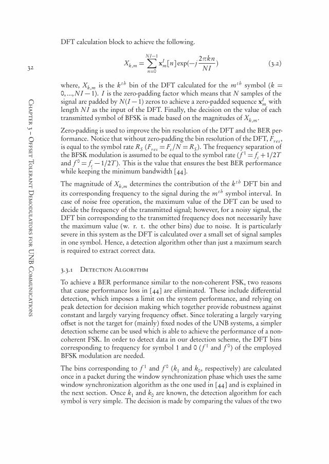
550999-L-bw-Siavash550999-L-bw-Siavash550999-L-bw-Siavash550999-L-bw-SiavashProcessed on: 23-11-2020Processed on: 23-11-2020Processed on: 23-11-2020Processed on: 23-11-2020 PDF page: 54PDF page: 54PDF page: 54PDF page: 54
32
Chapter3–OffsetTolerantDemodulatorsforUNBCommunications
DFT calculation block to achieve the following.
Xk ,m =N I−1∑
n=0
xIm[n]exp(− j
2πknN I
) (3.2)
where, Xk ,m is the k t h bin of the DFT calculated for the m t h symbol (k =0, ...,N I − 1). I is the zero-padding factor which means that N samples of thesignal are padded by N (I − 1) zeros to achieve a zero-padded sequence xI
m withlength N I as the input of the DFT. Finally, the decision on the value of eachtransmitted symbol of BFSK is made based on the magnitudes of Xk ,m .
Zero-padding is used to improve the bin resolution of the DFT and the BER per-formance. Notice that without zero-padding the bin resolution of the DFT, Fr e s ,is equal to the symbol rate RS (Fr e s = Fs/N = RS ). The frequency separation ofthe BFSK modulation is assumed to be equal to the symbol rate ( f 1 = fc+1/2Tand f 0 = fc − 1/2T ). This is the value that ensures the best BER performancewhile keeping the minimum bandwidth [44].
The magnitude of Xk ,m determines the contribution of the k t h DFT bin andits corresponding frequency to the signal during the m t h symbol interval. Incase of noise free operation, the maximum value of the DFT can be used todecide the frequency of the transmitted signal; however, for a noisy signal, theDFT bin corresponding to the transmitted frequency does not necessarily havethe maximum value (w. r. t. the other bins) due to noise. It is particularlysevere in this system as the DFT is calculated over a small set of signal samplesin one symbol. Hence, a detection algorithm other than just a maximum searchis required to extract correct data.
3.3.1 Detection Algorithm
To achieve a BER performance similar to the non-coherent FSK, two reasonsthat cause performance loss in [44] are eliminated. These include differentialdetection, which imposes a limit on the system performance, and relying onpeak detection for decision making which together provide robustness againstconstant and largely varying frequency offset. Since tolerating a largely varyingoffset is not the target for (mainly) fixed nodes of the UNB systems, a simplerdetection scheme can be used which is able to achieve the performance of a non-coherent FSK. In order to detect data in our detection scheme, the DFT binscorresponding to frequency for symbol 1 and 0 ( f 1 and f 0 ) of the employedBFSK modulation are needed.
The bins corresponding to f 1 and f 0 (k1 and k0, respectively) are calculatedonce in a packet during the window synchronization phase which uses the samewindow synchronization algorithm as the one used in [44] and is explained inthe next section. Once k1 and k0 are known, the detection algorithm for eachsymbol is very simple. The decision is made by comparing the values of the two

550999-L-bw-Siavash550999-L-bw-Siavash550999-L-bw-Siavash550999-L-bw-SiavashProcessed on: 23-11-2020Processed on: 23-11-2020Processed on: 23-11-2020Processed on: 23-11-2020 PDF page: 55PDF page: 55PDF page: 55PDF page: 55
33
3.3.2–WindowSynchronization
DFT Calc.
Window &Zero-Padding Detection
Synchronization
LPF
Timing
Figure 3.2: Block diagram of the DFT-based demodulator
DFT bins.
am =¨
+1 Xk1,m >Xk0,m
−1 Xk1,m <Xk0,m(3.3)
Figure 3.2 depicts the modified DFT-based demodulator. The window synchro-nization block determines the window timing, k0 and k1. The detection blockuses the DFT values and (3.3) to detect the received symbols.
3.3.2 Window Synchronization
As mentioned earlier, a DFT-based window synchronization algorithm has beenproposed in [44] which is necessary for proper functioning of the demodulatorin the presence of a large frequency offset. In this chapter, we also use the samewindow synchronization algorithm. Due to its effect on the complexity of theDFT-based demodulator, this algorithm is explained in detail in this section. Thisexplanation is also helpful to understand the method proposed in Chapter 5.
For synchronization, a preamble of alternating ones and zeros (1010...) is used.The number of symbols in the preamble is denoted by L. For each symbol, win-dows with different delay values, between 0 and N−1, are considered. Only oneof these windows is fully aligned and others include samples of two consecutivesymbols. Each window includes a sequence of samples as follows.
xm,i = [rm[i], ..., rm[N − 1], rm+1[0], ..., rm+1[i − 1]] (3.4)
The rm[i] is the same as in (3.1) while xm,i shows the set of samples for symbolm and window delay of i . The DFT is calculated for each set of samples asfollows.
X ik ,m =
N I−1∑
n=0
xIm,i [n]exp(− j
2πknN I
), (3.5)
where X ik ,m is the DFT value for the k t h bin and the m t h symbol when a window
with delay i is considered. xIm,i is the zero-padded sequence achieved from xm,i .

550999-L-bw-Siavash550999-L-bw-Siavash550999-L-bw-Siavash550999-L-bw-SiavashProcessed on: 23-11-2020Processed on: 23-11-2020Processed on: 23-11-2020Processed on: 23-11-2020 PDF page: 56PDF page: 56PDF page: 56PDF page: 56
34
Chapter3–OffsetTolerantDemodulatorsforUNBCommunications
DDelay=0
Delay=2
f0 f1
f0 f1
D
Delay=1
Delay=3
f0 f1
f0 f1
D
D
Delay=0Delay=1Delay=2Delay=3
Odd Symbols ( ) Even Symbols ( )
Figure 3.3: Three symbols of a preamble, the windows of different delay valuesfor the first two symbols and an example of spectrum variation when there are4 samples per symbol. Solid and dotted lines show windows and spectra of oddand even symbols, respectively.
Figure 3.3 illustrates three symbols of the preamble and the windows in caseof four samples per symbol (each square is a sample). It also shows how thespectrum varies for different delays. The double-headed arrows in the top partof the figure denote windows. Each row of arrows corresponds to a certain delayvalue as shown in the figure. Solid (dotted) arrows show the windows for an Odd(Even) symbol with different delay values. The symbols within the preambleare called Even and Odd depending on their index m = 1, ...L.
When X ik ,m is calculated for m = 1, .., L, k = 0, ...,N I −1 and i = 0, ...,N−1, for
each delay i , all DFTmagnitudes corresponding toOdd symbols (Even symbols)in the preamble are added together to achieve the following.
SOi (k) =
L/2∑
n=1
|X ik ,2n−1| (3.6)

550999-L-bw-Siavash550999-L-bw-Siavash550999-L-bw-Siavash550999-L-bw-SiavashProcessed on: 23-11-2020Processed on: 23-11-2020Processed on: 23-11-2020Processed on: 23-11-2020 PDF page: 57PDF page: 57PDF page: 57PDF page: 57
35
3.3.3–BERPerformanceandtheZero-paddingFactor
SEi (k) =
L/2∑
n=1
|X ik ,2n | (3.7)
In fact, (3.6) and (3.7) calculate the sumof theDFTmagnitudes for solidwindowsin Figure 3.3 and the sum of those for dotted windows with the same delay (orin each line of arrows as shown in Figure 3.3), respectively.
To synchronize the window, the delay value for which Ri in the following equa-tion is maximized needs to be found [44, 89].
Ri = [SEi (k
Ei )− SE
i (kOi )]+ [S
Oi (k
Oi )− SO
i (kEi )], (3.8)
where kEi and kO
i are the bins with maximum magnitude in SEi and SO
i , respec-tively. Finding the maximum of (3.9) is simply finding the delay value whichmaximizes the difference shown by D in Figure 3.3. In addition to the timing in-formation (window delay), the bins corresponding to two symbols are achievedas follows and sent to the detection block.
k1 = kOi and k0 = kE
i (3.9)
3.3.3 BER Performance and the Zero-padding Factor
Zero-padding is used to increase the bin resolution of the DFT and affects theBER performance of the DFT-based demodulator. Since the DFT is calculatedusing samples over a symbol, the bin resolution of theDFTwithout zero-paddingequals to the symbol rate (Fs/N = RS ). Since the frequency separation of theFSKmodulation is RS , the DFT bins corresponding to the two BFSK frequenciesare two adjacent bins in case of no zero-padding. Due to frequency offset, thefrequencies of the BFSK symbols may not match the DFT bins which leads tospectral leakage. In such cases, a low bin resolution causes erroneous detectionin presence of noise. The worst case is when the bins corresponding to the FSKsymbol frequencies are exactly in the middle of two DFT bins. The BER in thissituation depends on the bin resolution and can be improved by increasing thezero-padding factor.
To show the effect of the zero-padding factor on the BER performance, thedemodulator in Figure 3.2 is simulated for different zero-padding factors andthe worst case offset for that zero-padding. In these simulations, the preamblelength (L) and the number of samples per symbol (N ) are 16 and 8, respectively,similar to [44] (the BER performance for other values of N are discussed in thenext section). The BER curves for different zero-padding factors are shown inFigure 3.4. The BER curve for a non-coherent BFSK, which is the lower bound,is also demonstrated in Figure 3.4. According to Figure 3.4, at BER=0.1%, I = 8requires less than 5% more power compared to the non-coherent FSK. Thus, weuse I = 8 in the rest of this chapter.

550999-L-bw-Siavash550999-L-bw-Siavash550999-L-bw-Siavash550999-L-bw-SiavashProcessed on: 23-11-2020Processed on: 23-11-2020Processed on: 23-11-2020Processed on: 23-11-2020 PDF page: 58PDF page: 58PDF page: 58PDF page: 58
36
Chapter3–OffsetTolerantDemodulatorsforUNBCommunications
6 7 8 9 10 11 12 13 1410−6
10−510−5
10−4
10−3
10−2
10−1
100
Eb/N0[dB]
BER
Non-coherent FSKI=1I=2I=4I=8I=16
Figure 3.4: The BER performance of the DFT-based demodulator for differentzero-padding factors
3.4 Double Differential PSK
3.4.1 The Autocorrelation Based Demodulator
To eliminate the effect of the frequency offset on PSK detection, Double Dif-ferential signaling has been proposed [94] resulting in Double Differential PSK(DDPSK). The idea is an extension of the same idea for Differential PSK (DPSK).In DPSK, the phase of each symbol is compared with the phase of the previoussymbol to achieve robustness against constant phase offset. Now, to removethe effect of the frequency offset (a variable phase offset), we can add anotherdifferential encoder/decoder to the DPSK modulator/demodulator. An offsettolerant demodulator for DDPSK has been introduced based on the correlationof a signal with its delayed version. The is called Auto-Correlation Demodulator(ACD). The block diagram of an ACD for DDPSK is shown in Figure 3.5.
The baseband PSK signal after the Low-Pass Filter ( r (t ) in Figure 3.5) and duringthe n t h symbol period is as follows.
r (t ) =s
ES
Te j (ωO t+ϕn+θ0)+ n(t ), (3.10)
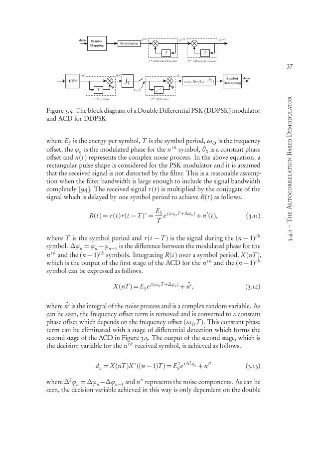
550999-L-bw-Siavash550999-L-bw-Siavash550999-L-bw-Siavash550999-L-bw-SiavashProcessed on: 23-11-2020Processed on: 23-11-2020Processed on: 23-11-2020Processed on: 23-11-2020 PDF page: 59PDF page: 59PDF page: 59PDF page: 59
37
3.4.1–TheAutocorrelationBasedDemodulator
Figure 3.5: The block diagram of a Double Differential PSK (DDPSK) modulatorand ACD for DDPSK
where ES is the energy per symbol, T is the symbol period,ωO is the frequencyoffset, the ϕn is the modulated phase for the n t h symbol, θ0 is a constant phaseoffset and n(t ) represents the complex noise process. In the above equation, arectangular pulse shape is considered for the PSK modulator and it is assumedthat the received signal is not distorted by the filter. This is a reasonable assump-tion when the filter bandwidth is large enough to include the signal bandwidthcompletely [94]. The received signal r (t ) is multiplied by the conjugate of thesignal which is delayed by one symbol period to achieve R(t ) as follows.
R(t ) = r (t )r (t −T )∗ =ES
Te j (ωO T+∆ϕn )+ n′(t ), (3.11)
where T is the symbol period and r (t − T ) is the signal during the (n − 1)t h
symbol. ∆ϕn = ϕn−ϕn−1 is the difference between the modulated phase for then t h and the (n− 1)t h symbols. Integrating R(t ) over a symbol period, X (nT ),which is the output of the first stage of the ACD for the n t h and the (n− 1)t h
symbol can be expressed as follows.
X (nT ) = ES e j (ωO T+∆ϕn )+ n′, (3.12)
where n′ is the integral of the noise process and is a complex random variable. Ascan be seen, the frequency offset term is removed and is converted to a constantphase offset which depends on the frequency offset (ωO T ). This constant phaseterm can be eliminated with a stage of differential detection which forms thesecond stage of the ACD in Figure 3.5. The output of the second stage, which isthe decision variable for the n t h received symbol, is achieved as follows.
dn =X (nT )X ∗((n− 1)T ) = E2S e j∆2ϕn + n′′ (3.13)
where∆2ϕn =∆ϕn−∆ϕn−1 and n′′ represents the noise components. As can beseen, the decision variable achieved in this way is only dependent on the double

550999-L-bw-Siavash550999-L-bw-Siavash550999-L-bw-Siavash550999-L-bw-SiavashProcessed on: 23-11-2020Processed on: 23-11-2020Processed on: 23-11-2020Processed on: 23-11-2020 PDF page: 60PDF page: 60PDF page: 60PDF page: 60
38
Chapter3–OffsetTolerantDemodulatorsforUNBCommunications
difference of ϕn . To be able to detect the transmitted information from thedecision variable in (3.13), the information is encoded in the double difference ofthe phases of the transmitted symbols. A double differential encoder for MPSKis depicted in Figure 3.5. From Figure 3.5 it can be concluded that, the encoderis achieved from cascading two differential encoders. Writing ϕn according toFigure 3.5, we have:
αn =βn −βn−1
βn = ϕn −ϕn−1 (3.14)
Using (6.1), it can be shown that the phase of dn (which is ∆2ϕn ) is actually αn .If dn is expressed as in (3.13), the transmitted symbol can be obtained using thefollowing decision criterion which is the same one used for conventional MPSKdetection [45].
αn = arg maxαi∈A
Re[dn × exp(− jαi )] (3.15)
where A= 2πiM |i = 0, ..., M − 1 is the set of possible symbol phases for MPSK
modulation. At least a 2 dB performance loss is the sacrifice compared to DPSK,to achieve frequency offset tolerance with DDPSK. A simple method to improvethe performance of the DDPSK technique is proposed in [94]. The improvementis achieved by changing the delay of the second stage of the double differentialencoder and the first stage of the ACD demodulator from T to 2T . This ex-tra delay changes the noise samples involved in the two stages of differentialdecoding and decreases their correlation [93]. As a result, the BER performanceimprovement is obtained without any additional complexity.
3.4.2 Synchronization for PSK
In the previous section, a window synchronization algorithm for the DFT-baseddemodulator for FSK was explained. The window synchronization algorithmis based on selecting the best set of samples. To have a fair comparison betweenthe complexity of the two methods, a synchronization algorithm for PSK isintroduced in this section and used in our simulations.
A discrete time model of a DDPSK demodulator in Figure 3.5 is shown in Figure3.6. It is assumed that sampling frequency is N times the symbol rate (there are Nsamples per symbol). The sampling frequency is proportional to the bandwidthof the LPF prior to the demodulator and also determines the offset tolerance ofthe filter (this will be discussed in the next section). For each incoming sampleat the input of the demodulator, a value is generated which is a sample of theoutput of the first stage. The summation (an integrate and dump filter) needs to
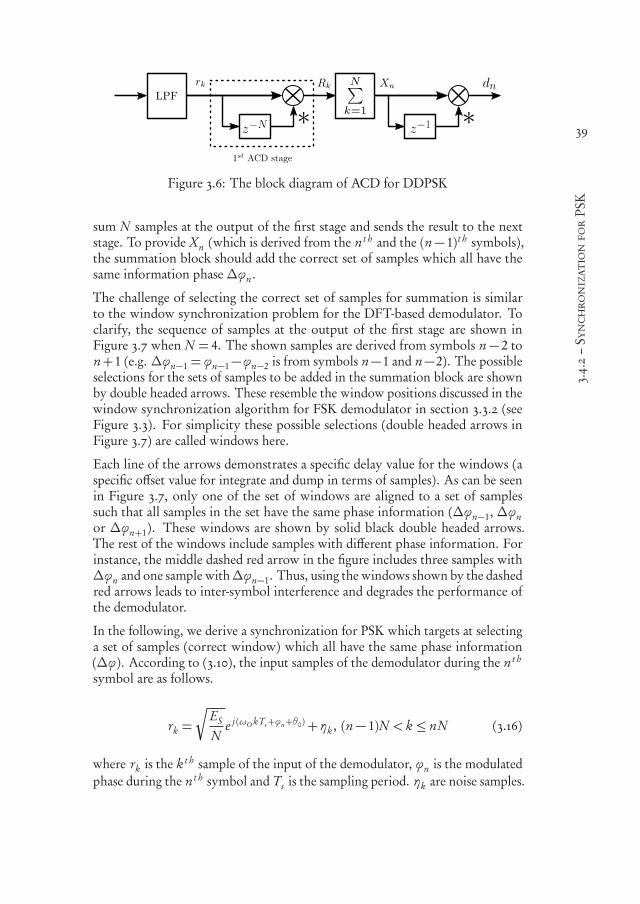
550999-L-bw-Siavash550999-L-bw-Siavash550999-L-bw-Siavash550999-L-bw-SiavashProcessed on: 23-11-2020Processed on: 23-11-2020Processed on: 23-11-2020Processed on: 23-11-2020 PDF page: 61PDF page: 61PDF page: 61PDF page: 61
39
3.4.2–SynchronizationforPSK
Figure 3.6: The block diagram of ACD for DDPSK
sum N samples at the output of the first stage and sends the result to the nextstage. To provide Xn (which is derived from the n t h and the (n−1)t h symbols),the summation block should add the correct set of samples which all have thesame information phase ∆ϕn .
The challenge of selecting the correct set of samples for summation is similarto the window synchronization problem for the DFT-based demodulator. Toclarify, the sequence of samples at the output of the first stage are shown inFigure 3.7 when N = 4. The shown samples are derived from symbols n− 2 ton+1 (e.g. ∆ϕn−1 = ϕn−1−ϕn−2 is from symbols n−1 and n−2). The possibleselections for the sets of samples to be added in the summation block are shownby double headed arrows. These resemble the window positions discussed in thewindow synchronization algorithm for FSK demodulator in section 3.3.2 (seeFigure 3.3). For simplicity these possible selections (double headed arrows inFigure 3.7) are called windows here.
Each line of the arrows demonstrates a specific delay value for the windows (aspecific offset value for integrate and dump in terms of samples). As can be seenin Figure 3.7, only one of the set of windows are aligned to a set of samplessuch that all samples in the set have the same phase information (∆ϕn−1, ∆ϕnor ∆ϕn+1 ). These windows are shown by solid black double headed arrows.The rest of the windows include samples with different phase information. Forinstance, the middle dashed red arrow in the figure includes three samples with∆ϕn and one sample with∆ϕn−1. Thus, using the windows shown by the dashedred arrows leads to inter-symbol interference and degrades the performance ofthe demodulator.
In the following, we derive a synchronization for PSK which targets at selectinga set of samples (correct window) which all have the same phase information(∆ϕ). According to (3.10), the input samples of the demodulator during the n t h
symbol are as follows.
rk =s
ES
Ne j (ωO kTs+ϕn+θ0)+ηk , (n− 1)N < k ≤ nN (3.16)
where rk is the k t h sample of the input of the demodulator, ϕn is the modulatedphase during the n t h symbol and Ts is the sampling period. ηk are noise samples.

550999-L-bw-Siavash550999-L-bw-Siavash550999-L-bw-Siavash550999-L-bw-SiavashProcessed on: 23-11-2020Processed on: 23-11-2020Processed on: 23-11-2020Processed on: 23-11-2020 PDF page: 62PDF page: 62PDF page: 62PDF page: 62
40
Chapter3–OffsetTolerantDemodulatorsforUNBCommunications
Figure 3.7: The sequence of samples at the output of the first stage. Doubleheaded arrows show the possible selections for the sets of samples to be addedin the summation block.
Using (3.11) and (3.16), the samples at the output of the first stage when the n t h
and the (n− 1)t h symbols are multiplied are as follows.
Rk = rk r ∗k−N =ES
Ne j (ωO T+∆ϕn )+η′k , (3.17)
where η′k represents the noise components. Every N samples, the phase of Rkchanges depending on the difference between themodulated phase of the receivedsymbols, ∆ϕn . A sequence of 3N samples of R is shown in Figure 3.8. Doubleheaded arrows show windows for three different delays, 0, d and N − 1. Thesums over the two first windows with delay d , which are shown by w1(d ) andw2(d ) are calculated as follows (assuming no noise).
w1(d ) =N+d∑
i=d+1
Ri
=N∑
i=d+1
ES
Ne j (ωO T+∆ϕn−1)+
N+d∑
i=N+1
ES
Ne j (ωO T+∆ϕn )
= (N − d )ES
Ne j (ωO T+∆ϕn−1)+ d
ES
Ne j (ωO T+∆ϕn ) (3.18)
w2(d ) =2N+d∑
i=N+d+1
Ri
=2N∑
i=N+d+1
ES
Ne j (ωO T+∆ϕn )+
2N+d∑
i=2N+1
ES
Ne j (ωO T+∆ϕn+1)
= (N − d )ES
Ne j (ωO T+∆ϕn )+ d
ES
Ne j (ωO T+∆ϕn+1) (3.19)
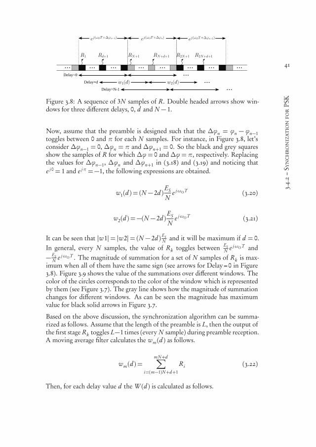
550999-L-bw-Siavash550999-L-bw-Siavash550999-L-bw-Siavash550999-L-bw-SiavashProcessed on: 23-11-2020Processed on: 23-11-2020Processed on: 23-11-2020Processed on: 23-11-2020 PDF page: 63PDF page: 63PDF page: 63PDF page: 63
41
3.4.2–SynchronizationforPSK
Delay=0
Delay=d
Delay=N-1
Figure 3.8: A sequence of 3N samples of R. Double headed arrows show win-dows for three different delays, 0, d and N − 1.
Now, assume that the preamble is designed such that the ∆ϕn = ϕn − ϕn−1toggles between 0 and π for each N samples. For instance, in Figure 3.8, let’sconsider ∆ϕn−1 = 0, ∆ϕn = π and ∆ϕn+1 = 0. So the black and grey squaresshow the samples of R for which ∆ϕ = 0 and ∆ϕ =π, respectively. Replacingthe values for ∆ϕn−1, ∆ϕn and ∆ϕn+1 in (3.18) and (3.19) and noticing thate j 0 = 1 and e jπ =−1, the following expressions are obtained.
w1(d ) = (N − 2d )ES
Ne jωO T (3.20)
w2(d ) =−(N − 2d )ES
Ne jωO T (3.21)
It can be seen that |w1|= |w2|= (N − 2d ) ESN and it will be maximum if d = 0.
In general, every N samples, the value of Rk toggles between ESN e jωO T and
− ESN e jωO T . The magnitude of summation for a set of N samples of Rk is max-
imum when all of them have the same sign (see arrows for Delay=0 in Figure3.8). Figure 3.9 shows the value of the summations over different windows. Thecolor of the circles corresponds to the color of the window which is representedby them (see Figure 3.7). The gray line shows how the magnitude of summationchanges for different windows. As can be seen the magnitude has maximumvalue for black solid arrows in Figure 3.7.
Based on the above discussion, the synchronization algorithm can be summa-rized as follows. Assume that the length of the preamble is L, then the output ofthe first stage Rk toggles L−1 times (every N sample) during preamble reception.A moving average filter calculates the wm(d ) as follows.
wm(d ) =mN+d∑
i=(m−1)N+d+1
Ri (3.22)
Then, for each delay value d the W (d ) is calculated as follows.

550999-L-bw-Siavash550999-L-bw-Siavash550999-L-bw-Siavash550999-L-bw-SiavashProcessed on: 23-11-2020Processed on: 23-11-2020Processed on: 23-11-2020Processed on: 23-11-2020 PDF page: 64PDF page: 64PDF page: 64PDF page: 64
42
Chapter3–OffsetTolerantDemodulatorsforUNBCommunications
Figure 3.9: The values of summation over different windows of Rk samples. Thecolors correspond to the window (arrow) colors in Figure 3.7.
W (d ) =L−2∑
m=1
|wm(d )| (3.23)
The delay value which maximizes the W (d ) is the correct delay and determinesthe proper set of samples for summation in Figure 3.6 to achieve Xn . Once thisvalue is determined during the preamble, it can be used for the rest of the packet.
3.5 Scaling Offset Tolerance (BER and Complexity Evalu-
ation)
3.5.1 BER and Offset Tolerance
Since the proposed method for FSK uses a window synchronization phase toacquire k0 and k1 (the bins corresponding to f 0 and f 1, respectively), the effectof frequency offset is already removed. As explained in the previous section,the Double Differential PSK (DDPSK) demodulator also eliminates the effect offrequency offset on the received signal. So in principle, both methods are capableof tolerating any value of frequency offset. As explained in Chapter 2, when anoffset tolerant demodulator is used, the main parameter which determines thefrequency offset tolerance is the bandwidth of the low-pass filter prior to thedemodulator. A filter with bandwidth BF (similar to Chapter 2) is shown inFigure 3.10. The sampling frequency (for complex samples) is set to Fs = 2BF = Fto avoid aliasing and noise folding. Bt indicates the transition band of the filterwhich is non-zero for practical filters. The signal bandwidth and the maximumtolerable frequency offset are shown by BS and ± fO,max , respectively.
If Bt = 0 (an ideal filter), the sampling frequency should meet the followingcriterion.
Fs ≥ BS + 2| fO,max | (3.24)

550999-L-bw-Siavash550999-L-bw-Siavash550999-L-bw-Siavash550999-L-bw-SiavashProcessed on: 23-11-2020Processed on: 23-11-2020Processed on: 23-11-2020Processed on: 23-11-2020 PDF page: 65PDF page: 65PDF page: 65PDF page: 65
43
3.5.1–BERandOffsetTolerance
Figure 3.10: The relation between signal bandwidth (BS ), sampling frequency(Fs ), filter bandwidth (BF ) and maximum tolerable frequency offset ( fO,max )
Here, we assume that the sampling frequency, Fs =N RS , is an integer multipleof the symbol rate RS (equal to the bit rate for BFSK) and N is the number ofsamples per symbol. Thus, according to (3.24), the amount of the frequencyoffset, which can be tolerated by the demodulator, is tuned only by changing thefilter bandwidth, BF (and N accordingly). The maximum tolerable frequencyoffset and the range of the normalized tolerable frequency offset can be obtainedas follows.
| fO,max |= RSN −BS/RS
2(3.25)
−N −BS/RS
2≤
fO
RS≤+
N −BS/RS
2(3.26)
The range of the tolerable frequency offset for each modulation scheme can beobtained by substituting the corresponding signal bandwidth in (3.26). Theapproximate null-to-null bandwidth (BS ) of BFSK is fs e p + 2RS [103] and, here,the frequency separation is assumed to be equal to the symbol rate ( fs e p = RS ).Thus, the range of the tolerable frequency offset normalized to the symbol ratefor BFSK is:
− N − 32≤
fO
RS≤+N − 3
2(3.27)
The offset tolerance of a DDPSK demodulator can be obtained in a similar wayby replacing BS with the null-to-null bandwidth of PSK which is 2RS whenrectangular pulse shaping is used [103]. It is worth mentioning that for a prac-tical filter, Bt = 0 which decreases the offset tolerance for the same samplingfrequency; nevertheless, using a larger BF to compensate for non-zero Bt andconsider Fs = 2BF extends offset tolerance to the desired value.

550999-L-bw-Siavash550999-L-bw-Siavash550999-L-bw-Siavash550999-L-bw-SiavashProcessed on: 23-11-2020Processed on: 23-11-2020Processed on: 23-11-2020Processed on: 23-11-2020 PDF page: 66PDF page: 66PDF page: 66PDF page: 66
44
Chapter3–OffsetTolerantDemodulatorsforUNBCommunications
6 7 8 9 10 11 12 13 1410−510−5
10−4
10−3
10−2
10−1
100
Non-Coherent FSKFSK FT=8FSK FT=16
DDPSK, FT = 1DDPSK, FT = 8DDPSK, FT = 16
Eb/N0[dB]
BER
Figure 3.11: The BER curves for DFT-Based and DDPSK demodulator in pres-ence of different filter bandwidths
In the following results, Fs = F and its value normalized to the symbol rate, F T ,is used for presenting the simulation results. The effect of increasing the filterbandwidth is modeled as increased noise bandwidth resulting in increased noisepower levels. The distortion of the filter is neglected which is reasonable forlarge bandwidths. To show the performance of the offset tolerant demodulatorsfor different filter bandwidths, the BER curves are derived for F T = 8,16. TheBER curves for the DFT-based FSK demodulator and the ACD for DDPSK areshown in Figure 3.11. The preamble length L is set to 16 for both demodulators.For DDPSK the BER curve for F T = 1 is also shown. Actually, F T = 1 isalso called coherent DDPSK when the LPF is exactly matched to the signal.However, this is not a realistic assumption in presence of a frequency offsetand rectangular pulse shape [94]. We use F T = 1 and no frequency offset as areference of the best BER performance of the DDPSK demodulator. Because ofthe minimum filter bandwidth the noise power at the input of the demodulatoris minimal as well [93]. Additionally, as a lower bound for the FSK demodulatorperformance, the BER curve of a non-coherent FSK demodulator [45] is alsoshown in Figure 3.11. It is the same as the non-coherent demodulator (correlatorbased demodulator) discussed in the previous chapter.
It can be seen that the BER curves for the DFT-Based demodulator match thoseof non-coherent BFSK detection. However, the BER performance of theDDPSKdegrades when the filter bandwidth increases. For F T = 1, DDPSK can achievea BER performance which is 1 dB better than the DFT-Based demodulator.
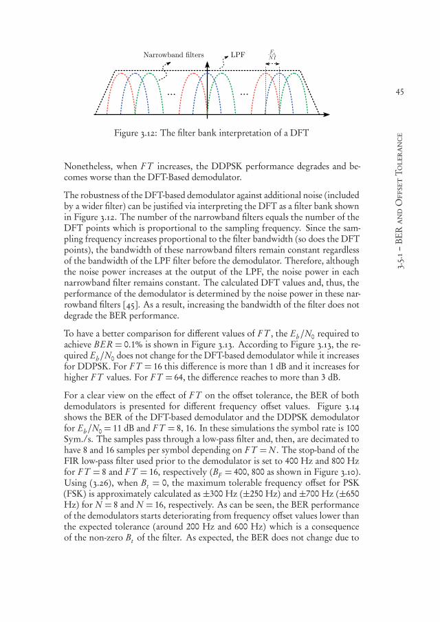
550999-L-bw-Siavash550999-L-bw-Siavash550999-L-bw-Siavash550999-L-bw-SiavashProcessed on: 23-11-2020Processed on: 23-11-2020Processed on: 23-11-2020Processed on: 23-11-2020 PDF page: 67PDF page: 67PDF page: 67PDF page: 67
45
3.5.1–BERandOffsetToleranceFigure 3.12: The filter bank interpretation of a DFT
Nonetheless, when F T increases, the DDPSK performance degrades and be-comes worse than the DFT-Based demodulator.
The robustness of the DFT-based demodulator against additional noise (includedby a wider filter) can be justified via interpreting the DFT as a filter bank shownin Figure 3.12. The number of the narrowband filters equals the number of theDFT points which is proportional to the sampling frequency. Since the sam-pling frequency increases proportional to the filter bandwidth (so does the DFTpoints), the bandwidth of these narrowband filters remain constant regardlessof the bandwidth of the LPF filter before the demodulator. Therefore, althoughthe noise power increases at the output of the LPF, the noise power in eachnarrowband filter remains constant. The calculated DFT values and, thus, theperformance of the demodulator is determined by the noise power in these nar-rowband filters [45]. As a result, increasing the bandwidth of the filter does notdegrade the BER performance.
To have a better comparison for different values of F T , the Eb/N0 required toachieve BER = 0.1% is shown in Figure 3.13. According to Figure 3.13, the re-quired Eb/N0 does not change for the DFT-based demodulator while it increasesfor DDPSK. For F T = 16 this difference is more than 1 dB and it increases forhigher F T values. For F T = 64, the difference reaches to more than 3 dB.
For a clear view on the effect of F T on the offset tolerance, the BER of bothdemodulators is presented for different frequency offset values. Figure 3.14shows the BER of the DFT-based demodulator and the DDPSK demodulatorfor Eb/N0 = 11 dB and F T = 8, 16. In these simulations the symbol rate is 100Sym./s. The samples pass through a low-pass filter and, then, are decimated tohave 8 and 16 samples per symbol depending on F T =N . The stop-band of theFIR low-pass filter used prior to the demodulator is set to 400 Hz and 800 Hzfor F T = 8 and F T = 16, respectively (BF = 400, 800 as shown in Figure 3.10).Using (3.26), when Bt = 0, the maximum tolerable frequency offset for PSK(FSK) is approximately calculated as ±300 Hz (±250 Hz) and ±700 Hz (±650Hz) for N = 8 and N = 16, respectively. As can be seen, the BER performanceof the demodulators starts deteriorating from frequency offset values lower thanthe expected tolerance (around 200 Hz and 600 Hz) which is a consequenceof the non-zero Bt of the filter. As expected, the BER does not change due to
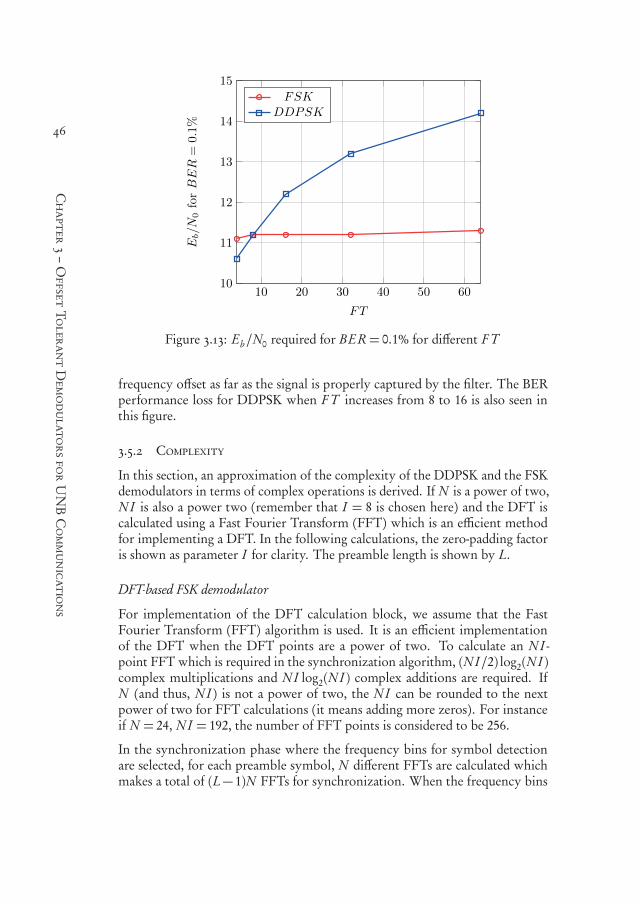
550999-L-bw-Siavash550999-L-bw-Siavash550999-L-bw-Siavash550999-L-bw-SiavashProcessed on: 23-11-2020Processed on: 23-11-2020Processed on: 23-11-2020Processed on: 23-11-2020 PDF page: 68PDF page: 68PDF page: 68PDF page: 68
46
Chapter3–OffsetTolerantDemodulatorsforUNBCommunications
10 20 30 40 50 6010
11
12
13
14
15
FT
Eb/N
0forBER
=0.1%
FSKDDPSK
Figure 3.13: Eb/N0 required for BER= 0.1% for different F T
frequency offset as far as the signal is properly captured by the filter. The BERperformance loss for DDPSK when F T increases from 8 to 16 is also seen inthis figure.
3.5.2 Complexity
In this section, an approximation of the complexity of the DDPSK and the FSKdemodulators in terms of complex operations is derived. If N is a power of two,N I is also a power two (remember that I = 8 is chosen here) and the DFT iscalculated using a Fast Fourier Transform (FFT) which is an efficient methodfor implementing a DFT. In the following calculations, the zero-padding factoris shown as parameter I for clarity. The preamble length is shown by L.
DFT-based FSK demodulator
For implementation of the DFT calculation block, we assume that the FastFourier Transform (FFT) algorithm is used. It is an efficient implementationof the DFT when the DFT points are a power of two. To calculate an N I -point FFT which is required in the synchronization algorithm, (N I/2) log2(N I )complex multiplications and N I log2(N I ) complex additions are required. IfN (and thus, N I ) is not a power of two, the N I can be rounded to the nextpower of two for FFT calculations (it means adding more zeros). For instanceif N = 24, N I = 192, the number of FFT points is considered to be 256.
In the synchronization phase where the frequency bins for symbol detectionare selected, for each preamble symbol, N different FFTs are calculated whichmakes a total of (L− 1)N FFTs for synchronization. When the frequency bins
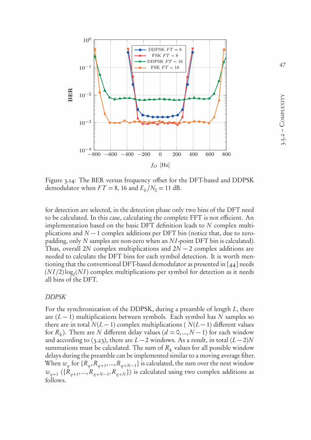
550999-L-bw-Siavash550999-L-bw-Siavash550999-L-bw-Siavash550999-L-bw-SiavashProcessed on: 23-11-2020Processed on: 23-11-2020Processed on: 23-11-2020Processed on: 23-11-2020 PDF page: 69PDF page: 69PDF page: 69PDF page: 69
47
3.5.2–Complexity
−800 −600 −400 −200 0 200 400 600 80010−4
10−3
10−2
10−1
100
fO [Hz]
BER
DDPSK FT = 8
FSK FT = 8
DDPSK FT = 16
FSK FT = 16
Figure 3.14: The BER versus frequency offset for the DFT-based and DDPSKdemodulator when F T = 8, 16 and Eb/N0 = 11 dB.
for detection are selected, in the detection phase only two bins of the DFT needto be calculated. In this case, calculating the complete FFT is not efficient. Animplementation based on the basic DFT definition leads to N complex multi-plications and N − 1 complex additions per DFT bin (notice that, due to zero-padding, only N samples are non-zero when an N I -point DFT bin is calculated).Thus, overall 2N complex multiplications and 2N − 2 complex additions areneeded to calculate the DFT bins for each symbol detection. It is worth men-tioning that the conventional DFT-based demodulator as presented in [44] needs(N I/2) log2(N I ) complex multiplications per symbol for detection as it needsall bins of the DFT.
DDPSK
For the synchronization of the DDPSK, during a preamble of length L, thereare (L− 1) multiplications between symbols. Each symbol has N samples sothere are in total N (L− 1) complex multiplications ( N (L− 1) different valuesfor Rk ). There are N different delay values (d = 0, ...,N − 1) for each windowand according to (3.23), there are L− 2 windows. As a result, in total (L− 2)Nsummations must be calculated. The sum of Rk values for all possible windowdelays during the preamble can be implemented similar to a moving average filter.When wq for Rq , Rq+1, ..., Rq+N−1 is calculated, the sum over the next windowwq+1 (Rq+1, ..., Rq+N−1, Rq+N ) is calculated using two complex additions asfollows.
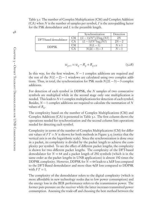
550999-L-bw-Siavash550999-L-bw-Siavash550999-L-bw-Siavash550999-L-bw-SiavashProcessed on: 23-11-2020Processed on: 23-11-2020Processed on: 23-11-2020Processed on: 23-11-2020 PDF page: 70PDF page: 70PDF page: 70PDF page: 70
48
Chapter3–OffsetTolerantDemodulatorsforUNBCommunications
Table 3.1: The number of Complex Multiplication (CM) and Complex Addition(CA) when N is the number of samples per symbol, I is the zero-padding factorfor the FSK demodulator and L is the preamble length.
Synchronization Detection
DFT-based demodulator CM ((L− 1)I N 2)/2 log2(N I ) 2NCA (L− 1)I N 2 log2(N I ) 2N − 2
DDPSK CM N (L− 1) N + 1CA N (2L− 3)− 3 N − 1
wq+1 = wq −Rq +Rq+N (3.28)
In this way, for the first window, N − 1 complex additions are required andthe rest of the N (L− 2)− 1 windows are calculated using two complex addi-tions. Thus, in total, the synchronization for PSK needs N (2L− 3)− 3 complexadditions.
For detection of each symbol in DDPSK, the N samples of two consecutivesymbols are multiplied while in the second stage only one multiplication isneeded. This leads to N+1 complexmultiplications for detection of each symbol.Besides, N − 1 complex additions are required to calculate the summation of Nvalues of Rk .
The complexity based on the number of Complex Multiplications (CM) andComplex Additions (CA) is presented in Table 3.1. The first column shows theoperations needed for synchronization and the second column lists operationsneeded for detecting each symbol.
Complexity in terms of the number of Complex Multiplications (CM) for differ-ent values of F T =N is shown for both methods in Figure 3.15 (notice that thevertical axis is on the logarithmic scale). Since the synchronization is done oncein a packet, its complexity is divided by the packet length to achieve the com-plexity per symbol. To see the effect of different packet lengths, the complexityis shown for two different packet lengths. The complexity of the DFT-baseddemodulator for N = 64 and a packet length of 250 symbols (which is in thesame order as the packet lengths in UNB applications) is almost 150 times theDDPSK complexity. However, DDPSK for N = 64 leads to a 3dB loss comparedto the DFT-Based demodulator and more than 4dB loss compared to DDPSKwith F T = 1.
The complexity of the demodulator refers to the digital complexity (which ismore affordable in new technology nodes due to low power consumption) andthe energy loss in the BER performance refers to the transmission power. Theformer puts pressure on the receiver while the latter increases transmitted powerconsumption. Assessing the trade-off and choosing the best method between the

550999-L-bw-Siavash550999-L-bw-Siavash550999-L-bw-Siavash550999-L-bw-SiavashProcessed on: 23-11-2020Processed on: 23-11-2020Processed on: 23-11-2020Processed on: 23-11-2020 PDF page: 71PDF page: 71PDF page: 71PDF page: 71
49
3.6–Conclusion
10 20 30 40 50 60100
101
102
103
104
FT
NumberofCM
persy
mbol
FSK 250 Sym.FSK 1000 Sym.
DDPSK 250 Sym.DDPSK 1000 Sym.
Figure 3.15: The number of complex multiplications required for calculatingeach symbol
DDPSK and DFT-Based demodulator, needs to take various parameters of thespecific target application into account and can be decided at design time.
FSK and PSK both are used in UNB applications and the behavior of the in-vestigated demodulators shows that they are two extreme cases; large BER per-formance degradation (PSK) and significant complexity (FSK). This raises aninteresting question: is it possible to modify these two demodulators such thattheir limitations become milder and both can be efficiently used if required?This means finding a less complex design for the DFT-Based demodulator (withminor or no sacrifice in the BER performance) and improving the BER perfor-mance of DDPSK compared to what is achievable now. These questions areanswered in the next two chapters by proposing two different techniques. Onealleviates the Eb/N0 loss in DDPSK when a wide filter is used and the otherfocuses on an efficient implementation of the DFT-Based demodulator.
3.6 Conclusion
This chapter investigated two offset tolerant demodulators for FSK and PSKwhich are capable of tolerating a large frequency offset (multiple times the sym-bol rate). For FSK, a DFT-based demodulator was designed using a simpledetection method. To synchronize the DFT window in the presence of a largefrequency offset, an existing DFT-based window synchronization was utilized.For PSK, a Double Differential scheme (DDPSK) and an autocorrelation baseddemodulator (ACD) were considered. To ensure a fair complexity comparisonbetween these two demodulators, a synchronization scheme for the DDPSK was

550999-L-bw-Siavash550999-L-bw-Siavash550999-L-bw-Siavash550999-L-bw-SiavashProcessed on: 23-11-2020Processed on: 23-11-2020Processed on: 23-11-2020Processed on: 23-11-2020 PDF page: 72PDF page: 72PDF page: 72PDF page: 72
50
Chapter3–OffsetTolerantDemodulatorsforUNBCommunications
considered as well. These demodulators with their synchronization schemeswere simulated for different filter bandwidths and their BER performance andcomplexity were compared. It was seen that the DFT-based demodulator is ro-bust against increased noise bandwidth due to a wider filter while imposing con-siderable complexity. In contrast, DDPSK provides a low complexity solutionwhich is sensitive to the filter bandwidth and has significant BER performancedegradation in case of large filters (more than 2 dB loss when F T changes from1 to 16). In the next two chapters, two solutions are proposed to overcome theselimitations of the DFT-Based demodulator and DDPSK.

550999-L-bw-Siavash550999-L-bw-Siavash550999-L-bw-Siavash550999-L-bw-SiavashProcessed on: 23-11-2020Processed on: 23-11-2020Processed on: 23-11-2020Processed on: 23-11-2020 PDF page: 73PDF page: 73PDF page: 73PDF page: 73
51

550999-L-bw-Siavash550999-L-bw-Siavash550999-L-bw-Siavash550999-L-bw-SiavashProcessed on: 23-11-2020Processed on: 23-11-2020Processed on: 23-11-2020Processed on: 23-11-2020 PDF page: 74PDF page: 74PDF page: 74PDF page: 74
52

550999-L-bw-Siavash550999-L-bw-Siavash550999-L-bw-Siavash550999-L-bw-SiavashProcessed on: 23-11-2020Processed on: 23-11-2020Processed on: 23-11-2020Processed on: 23-11-2020 PDF page: 75PDF page: 75PDF page: 75PDF page: 75
534Shifted Correlation
Demodulator for DDPSK
Abstract – The autocorrelation based demodulator (ACD) for DDPSK is ademodulator which can tolerate frequency offset. However, to tolerate a largefrequency offset, the bandwidth of the low-pass filter before the demodulatormust increase. It was shown in the previous chapter that this increased filterbandwidth leads to a larger noise bandwidth and degrades BER performance.In this chapter, a new method is proposed to overcome this problem. Insteadof one path of ACD, samples at the output of the filter go through multiplepaths with adjusted delay and summation blocks in the ACD. The sum ofthe outputs of these paths provide the input to the detector with an increasedSNR compared to the conventional structure. Using the proposed method, theEb/N0 required for a specific BER remains independent of the filter bandwidthif the target BER is less than 0.01.
4.1 Introduction
The autocorrelation based demodulator (ACD) for second-order differentialPSK also known as Double Differential PSK (DDPSK) has been introduced asa demodulator which can detect phase information independent of frequencyoffset [93]. As explained in the previous chapter, when using an offset tolerantdemodulator, the bandwidth of the filter before the demodulator should increasein accordance with the desired range of the frequency offset tolerance. On theother hand, as the noise bandwidth is proportional to the filter bandwidth, theBER performance deteriorates when filter bandwidth increases [94].
In our search for demodulator scalability in terms of frequency offset tolerance,a novel method is proposed in this chapter. The proposed method can overcome
This chapter is based on [S:4].
550999-L-bw-Siavash550999-L-bw-Siavash550999-L-bw-Siavash550999-L-bw-SiavashProcessed on: 23-11-2020Processed on: 23-11-2020Processed on: 23-11-2020Processed on: 23-11-2020 PDF page: 76PDF page: 76PDF page: 76PDF page: 76
54
Chapter4–ShiftedCorrelationDemodulatorforDDPSK
the effect of the increased noise bandwidth when widening the filter prior to theDDPSK demodulator. As a result, increasing the range of offset tolerance doesnot lead to BER performance degradation which is the case for the conventionalmethod. In addition to simulations, a mathematical approach is followed toanalyze noise components and to prove effectiveness of the proposed method.
In the next section, the proposed demodulators for DDPSK are briefly reviewed.Before explicating the proposed method, a conventional ACD for DDPSK isinvestigated in section 4.3 to achieve a clear view on the reason of the BERperformance degradation. This overview takes us to section 4.4 and 4.5 whichelaborate on the proposed method and its BER performance, respectively. Sim-ulation results are presented in section 4.6. Although the method improves theBER performance, it adds complexity. The trade-off between BER performanceand complexity is investigated in section 4.7 and concluding remarks are drawnin the last part of this chapter, section 4.8.
4.2 Related Work
The ACD for DDPSK can tolerate frequency offset at the expense of BER per-formance degradation compared to BPSK and DPSK. Different methods havebeen proposed to improve the performance of DDPSK and make its BER closerto DPSK or BPSK. A Generalized Likelihood detector and Maximum a Poste-riori (MAP) detector for DDPSK are investigated in [98, 99]. It is shown thatthese methods are identical to the simple heuristic detector (which is the samedetection scheme used in the autocorrelation based demodulator in the previouschapter). In [84] a variation of a DDPSK demodulator is introduced wherethe integrator is prior to the differential detection. Moreover, the differentialdetection is replaced with a multiple symbol sequence detection. Although thismethod improves the BER performance, it only works when the frequency offsetis less than 25% of the data rate.
In [94], the second stage of the DDPSK after the integrator is replaced with amultiple symbol detector for DPSK. In [12], a Maxmimum Likelihood metricis achieved for multiple symbol detecton of DDPSK which is independent ofthe frequency offset. To get close to the DPSK performance, these methodsconsiderably increase complexity. As a simpler solution, a Decision-Feedbackbased detection is proposed in [49] which uses the previously detected symbolsto improve the demodulator performance. Using proper weighting factors inthe feedback loops, a BER performance close to coherent BPSK can be achieved.
All of the abovemethods bridge the gap in the performance of DDPSK and BPSKto some extent; however, all of them will experience a performance loss in caseof a large frequency offset and wider filter. This loss is not due to the variablephase (as it is solved with all of these methods) but as a consequence of theincreased noise bandwidth. Methods in [12, 49], mentioned above, are affectedmuch worse than a conventional ACD by a wide filter. These methods rely on a

550999-L-bw-Siavash550999-L-bw-Siavash550999-L-bw-Siavash550999-L-bw-SiavashProcessed on: 23-11-2020Processed on: 23-11-2020Processed on: 23-11-2020Processed on: 23-11-2020 PDF page: 77PDF page: 77PDF page: 77PDF page: 77
55
4.3–ProblemStatement
single sample representation of the signal. The single sample representation withmatched filter is only valid if the frequency offset is very small. If the bandwidthof the low-pass filter prior to the demodulator increases, the noise variance ofthe sample increases proportional to the bandwidth of the filter.
For example, with the method proposed in [12], the BER of DDPSK becomesalmost equal to the BER of the coherent BPSK with the same SNR (of coursewith much higher complexity by increasing the observation length). The BERcurve of the coherent BPSK is actually the lower bound for the samples withthat SNR. However, when a wider filter is used, the Eb/N0 required to havethe same SNR at the demodulator input is increased proportionally to the filterbandwidth. Thus, increasing the filter bandwidth by a factor of two leads to3 dB SNR degradation for the same Eb/N0. As a consequence, the mentionedlower bound will be shifted by 3 dB making it almost the same as DDPSK [12].Therefore, although these methods are effective in case of a filter bandwidthequal or close to the signal bandwidth (i.e. frequency offset less than the symbolrate) their performance degrades drastically when the filter becomes wider.
In contrast, the conventional autocorrelation based demodulator (ACD) [93, 94]does not assume a single sample representation. In ACD for DDPSK we canuse more than one sample (the number of samples per symbol depends on thebandwidth of the filter). Then, the final filtering is actually the integration whichis done after the first stage of autocorrelation. This filter (integrator) is matchedto the signal (if a rectangular pulse is used) as the samples have zero frequencyafter the first autocorrelation stage. As a result, a conventional ACD for DDPSKfaces less drastic performance loss when the filter bandwidth increases. However,it still performs poorly when the filter bandwidth becomes several times thesymbol rate and it needs to be modified for tolerating large frequency offset. Inthe next section, we focus on distribution of noise components in the outputsof the first and the second stage of the ACD. The problem is defined based onthis understanding which helps us to explain our proposed method.
4.3 Problem Statement
The block diagrams of a double differential encoder and an autocorrelation baseddemodulator (ACD) for Double Differential PSK with a low-pass filter priorto the demodulator are shown in Figure4.1 (at the top and the bottom of thefigure, respectively). This is the same as what was introduced in Chapter 3.The double differential encoder puts the information in the double difference ofthe transmitted symbol phase. The received samples of the double differentiallyencoded signal are filtered and pass through two consecutive differential decoders.The first stage of the ACD converts the frequency offset to a constant phase offsetby correlating each symbol with the previous symbol. Subsequently, the secondstage removes the remaining phase offset [93]. Thus, the effect of frequencyoffset is removed from the final decision variable dn .

550999-L-bw-Siavash550999-L-bw-Siavash550999-L-bw-Siavash550999-L-bw-SiavashProcessed on: 23-11-2020Processed on: 23-11-2020Processed on: 23-11-2020Processed on: 23-11-2020 PDF page: 78PDF page: 78PDF page: 78PDF page: 78
56
Chapter4–ShiftedCorrelationDemodulatorforDDPSK
Figure 4.1: Block diagram of a double differential encoder with phase relationsand an ACD for DDPSK, T is the symbol period, N is the number of samplesper symbol and (∗) denotes complex conjugate.
As mentioned in Chapter 3, a simple modification to DDPSK, which is achievedwithout additional complexity, was introduced in [94]. It is obtained by in-creasing the delay of the second stage of the encoder and the first stage of thedemodulator in Figure 4.1 by one symbol period (changing T to 2T and z−N
to z−2N , respectively). In the following calculations and the proposed model,a single delay element and z−N is used (the T -T method) for the simplicity ofpresentation. However, it can be applied to the model with double delay andz−2N (the T -2T method) by only changing the delay values accordingly.
Considering the discussion in Chapter 3, it is assumed that the signal passesthrough a low-pass filter with a bandwidth of BF before the demodulator. Theminimum sampling rate after the filter must be F = 2BF (according to theNyquist theorem) for complex samples. Similar to [94], F is assumed to beequal to an integer multiple of the symbol rate and we use its value normalizedto the symbol rate F T (where T is the symbol period). Thus, there are F T =Ncomplex samples per symbol after the filter and at the input of the ACD. Con-sidering an AWGN channel and a filter bandwidth BF = F /2, such a samplingfrequency ensures that noise samples are uncorrelated for all N samples per sym-bol. In case of zero frequency offset, LPF can be replaced with a matched filterto maximize the SNR before the demodulator and one sample per symbol is sentto the demodulator (which will be two consecutive differential decoders). Thiscase is shown by F T = 1 and has the best BER performance. In the presence ofa large frequency offset, a wider filter is required so F >> 1/T .
The baseband representation of the samples of a phase modulated signal (PSK,

550999-L-bw-Siavash550999-L-bw-Siavash550999-L-bw-Siavash550999-L-bw-SiavashProcessed on: 23-11-2020Processed on: 23-11-2020Processed on: 23-11-2020Processed on: 23-11-2020 PDF page: 79PDF page: 79PDF page: 79PDF page: 79
57
4.3–ProblemStatement
DPSK or DDPSK) at the input of the demodulator (see Figure 4.1) during then t h symbol is:
rk ,n = sk ,n e j (ωO kTs+θ)+ηk ,n (4.1)
where rk ,n is the k t h sample from the n t h symbol (k = 1, ...,N ). Consideringrectangular pulse shaping and neglecting ISI (which is reasonable for large BF ),sk ,n = sn = e jϕn where ϕn = 2πi/M , i = 1,2, . . . , M − 1 for MPSK. ωO = 2π fOis the frequency offset, Ts is the sampling period and θ is a constant phase offset.Without loss of generality the signal amplitude is considered to be one to simplifynotations. The ηk ,n components for all k are independent circularly symmetricGaussian random variables with σ2 =Nσ2
1 where σ21 is the noise power in case
of F T = 1. In other words, real and imaginary parts of ηk ,n are independentGaussian random variablesN (0,Nσ2
1/2). The factor N in σ2 is due to the factthat the noise bandwidth when F T =N is N times the noise bandwidth in caseof F T = 1.
In an ACD, the received samples of consecutive symbols are correlated over asymbol period. This provides the output of the first stage of the ACD as follows.
Xn =N∑
k=1
rk ,n r ∗k ,n−1 = Sn +(Hs )n +(Hη)n (4.2)
where:
Sn =N∑
k=1
sn s∗n−1e jωO N Ts (4.3)
(Hs )n =N∑
k=1
(snη∗k ,n−1+ s∗n−1ηk ,n) (4.4)
(Hη)n =N∑
k=1
ηk ,nη∗k ,n−1 (4.5)
Sn is the only signal component and its power is N 2 (proportional to the magni-tude of the signal component). (Hs )n is the sum of signal-by-noise components.Since all noise samples are independent, all the components in the second summa-tion are independent randomvariablesCN (0,σ2) or equivalentlyCN (0,Nσ2
1 ).Thus, (Hs )n is in total aCN (0,2Nσ2) random variable. The ratio of the powerof the signal component to the power of (Hs )n (which is part of noise) is equal toN/2σ2 = 1/2σ2
1 . This ratio does not change with N . Thus, it can be concludedthat the other noise component i.e. (Hη)n is responsible for the performancedegradation when N increases. As (Hη)n is the multiplication of two Gaussiancomplex random variables, it is not Gaussian anymore. The details about thedistribution of the noise-by-noise component is mathematically explained in sec-tion 4.5. The next section elaborates on the proposed demodulator to overcomethis N = F T -dependent noise term.
550999-L-bw-Siavash550999-L-bw-Siavash550999-L-bw-Siavash550999-L-bw-SiavashProcessed on: 23-11-2020Processed on: 23-11-2020Processed on: 23-11-2020Processed on: 23-11-2020 PDF page: 80PDF page: 80PDF page: 80PDF page: 80
58
Chapter4–ShiftedCorrelationDemodulatorforDDPSK
4.4 The Proposed Demodulator
According to the previous section the third term of Xn in (4.2) is responsible foran increase is the noise power which is dependent on N . Assume that more repli-cas of the final decision variable are generated with correlated signal componentsand uncorrelated (Hη) components. Then, a final decision variable achieved byadding these replicas has a better effective SNR because of the coherent additionof signal components and the incoherent addition of (Hη) components. For thispurpose, we start with generating replicas of Xn (using the existing samples) forwhich the signal terms are correlated and terms resulting from noise-by-noisemultiplications are uncorrelated. In this section, the concept is explained and,in the next section, the effectiveness of the proposed method is shown mathe-matically.
Let’s start with the first stage of autocorrelation. The basic idea is illustrated inFigure 4.2. The (n − 1)t h and the n t h symbols are shown in this figure. Eachsquare shows one sample of a symbol and, in the figure, four samples per symbolare considered. In the first row under the symbols, the calculation of Xn as in theconventional demodulator is shown. In this case the samples are aligned in bothsymbols i.e. rk ,n−1 is multiplied by rk ,n . Now consider a one sample increase inthe delay of the first stage decoder (shown in the second row). It is equivalentto shifting the samples of the (n− 1)t h symbol to the right for one sample withrespect to the samples of the n t h symbol and then do the multiplications. Thisgenerates X R
n, p |p=1 in Figure 4.2. In the same way, by decreasing the delay byone sample (shifting the (n − 1)t h symbol to the left), X L
n, p |p=1 is calculated.It should be noticed that by shifting symbols by one sample, the number ofmultiplications decreases to N − 1 and X R
n, p |p=1 and X Ln, p |p=1 are the sum of
N − 1 terms.
Shifting and correlating can be extended to a shift of p samples to the rightor left to achieve X R
n, p and X Ln, p , respectively. This is actually increasing and
decreasing (respectively for X Rn, p and X L
n, p ) the delay of N samples in Figure 4.1while adjusting the limits of the summation block to make sure that each termin the summation corresponds to the same pair of symbols. It is, indeed, addingduplicate paths of correlation between the signal and its delayed versions withadjusted delay and summation blocks. X R
n, p and X Ln, p can be written as follows.
X Rn, p =
N∑
k=p+1
rk ,n r ∗k−p,n−1 = SRn, p +(Hs )
Rn, p +(Hη)
Rn, p (4.6)
X Ln, p =
N−p∑
k=1
rk ,n r ∗k+p,n−1 = SLn, p +(Hs )
Ln, p +(Hη)
Ln, p (4.7)

550999-L-bw-Siavash550999-L-bw-Siavash550999-L-bw-Siavash550999-L-bw-SiavashProcessed on: 23-11-2020Processed on: 23-11-2020Processed on: 23-11-2020Processed on: 23-11-2020 PDF page: 81PDF page: 81PDF page: 81PDF page: 81
59
4.4–TheProposedDemodulator
Figure 4.2: The concept of the first stage in the proposed demodulator
where SRn, p and SL
n, p are the signal components; (Hs )Rn, p and (Hs )
Rn, p are the noise-
by-signal components and (Hη)Rn, p and (Hη)
Ln, p are the noise-by-noise compo-
nents as defined in the following equations.
SRn, p =
N∑
k=p+1
sk ,n e j (ωkTs+θ) s∗k−p,n−1e− j (ω(kTs−(N+p)Ts )+θ) (4.8)
SLn, p =
N−p∑
k=1
sk ,n e j (ωkTs+θ) s∗k+p,n−1e− j (ω(kTs−(N−p)Ts )+θ) (4.9)
(Hs )Rn, p =
N∑
k=p+1
(sk ,nη∗k−p,n−1+ s∗k−p,n−1ηk ,n) (4.10)
(Hs )Ln, p =
N−p∑
k=1
(sk ,nη∗k+p,n−1+ s∗k+p,n−1ηk ,n) (4.11)
(Hη)Rn, p =
N∑
k=p+1
ηk ,nη∗k−p,n−1 (4.12)
550999-L-bw-Siavash550999-L-bw-Siavash550999-L-bw-Siavash550999-L-bw-SiavashProcessed on: 23-11-2020Processed on: 23-11-2020Processed on: 23-11-2020Processed on: 23-11-2020 PDF page: 82PDF page: 82PDF page: 82PDF page: 82
60
Chapter4–ShiftedCorrelationDemodulatorforDDPSK
(Hη)Ln, p =
N−p∑
k=1
ηk ,nη∗k+p,n−1 (4.13)
The terms SRn, p and SL
n, p for all p are correlated. In the previous section, weshowed that the ratio of the power of the signal component to the power of(Hs )n is independent of N ; thus, let us just focus on (Hη)
Rn, p and (Hη)
Ln, p here
((Hs )Ln, p and (Hs )
Rn, p will be discussed in the next section). Each term constituting
(Hη)Rn, p and (Hη)
Ln, p is a multiplication of two different and independent Gaussian
complex random variables. These new random variables are independent and adetailed discussion about their distribution follows in the next section.
For now, it can be seen that the shifted correlation outputs (X Rn, p and X L
n, p )provide us with more replicas of Xn with correlated signal components andindependent noise-by-noise components. Hence, adding X R
n, p and X Ln, p for all p
can lead to a decision metric with higher effective SNR. There is only one issueleft that must be taken into account.
Assuming a signal model similar to (4.1), SRn, p and SL
n, p are as follows.
SRn, p =
N∑
k=p+1
e j (∆ϕn )e j (ωO (N+p)Ts ) (4.14)
SLn, p =
N−p∑
k=1
e j (∆ϕn )e j (ωO (N−p)Ts ) (4.15)
where ∆ϕn = ϕn − ϕn−1 and Ts is the sampling period. As can be seen, theconstant phase offset is removed but there is still a phase offset at the output ofthe first stage (ωO (N ± p)Ts ) which depends on ωO , p and the direction of theshift (R or L).
IfωO = 0, the phases of all signal components are equal to∆ϕn . Thus, all X R(L)n, p
(which means X Rn, p or X L
n, p ) can be added to make a decision variable to detect∆ϕn . This will work if a DPSK is used and is capable of achieving an effectiveSNR equal to the SNR in case of F T = 1 (this will be shown in section 4.5).Improved SNR assures a BER performance practically independent of the filterbandwidth.
If ωO = 0, since this constant phase term (ωO (N ± p)Ts ) depends on p, itis not possible to simply add all X R(L)
n, p and send them to the next stage of theACD. Therefore, for each p and direction of shift, the shifted correlation of thesymbols n and n−1 (X R(L)
n, p ) must be first correlated with the shifted correlationof the symbols n−1 and n−2 (X R(L)
n−1, p ). This second stage is visualized in Figure4.3.
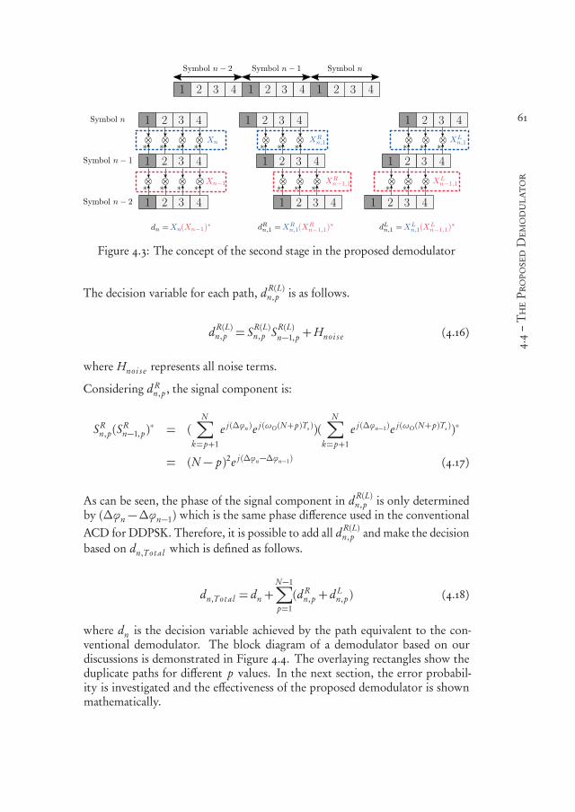
550999-L-bw-Siavash550999-L-bw-Siavash550999-L-bw-Siavash550999-L-bw-SiavashProcessed on: 23-11-2020Processed on: 23-11-2020Processed on: 23-11-2020Processed on: 23-11-2020 PDF page: 83PDF page: 83PDF page: 83PDF page: 83
61
4.4–TheProposedDemodulator
Figure 4.3: The concept of the second stage in the proposed demodulator
The decision variable for each path, d R(L)n, p is as follows.
d R(L)n, p = SR(L)
n, p SR(L)n−1, p +Hnoi s e (4.16)
where Hnoi s e represents all noise terms.
Considering d Rn, p , the signal component is:
SRn, p (S
Rn−1, p )
∗ = (N∑
k=p+1
e j (∆ϕn )e j (ωO (N+p)Ts ))(N∑
k=p+1
e j (∆ϕn−1)e j (ωO (N+p)Ts ))∗
= (N − p)2e j (∆ϕn−∆ϕn−1) (4.17)
As can be seen, the phase of the signal component in d R(L)n, p is only determined
by (∆ϕn −∆ϕn−1) which is the same phase difference used in the conventionalACD for DDPSK. Therefore, it is possible to add all d R(L)
n, p and make the decisionbased on dn,T ot al which is defined as follows.
dn,T ot al = dn +N−1∑
p=1
(d Rn, p + d L
n, p ) (4.18)
where dn is the decision variable achieved by the path equivalent to the con-ventional demodulator. The block diagram of a demodulator based on ourdiscussions is demonstrated in Figure 4.4. The overlaying rectangles show theduplicate paths for different p values. In the next section, the error probabil-ity is investigated and the effectiveness of the proposed demodulator is shownmathematically.

550999-L-bw-Siavash550999-L-bw-Siavash550999-L-bw-Siavash550999-L-bw-SiavashProcessed on: 23-11-2020Processed on: 23-11-2020Processed on: 23-11-2020Processed on: 23-11-2020 PDF page: 84PDF page: 84PDF page: 84PDF page: 84
62
Chapter4–ShiftedCorrelationDemodulatorforDDPSK
Figure 4.4: Block diagram of the proposed demodulator for DDPSK
4.5 Error Probability
The proposed method is designed for DDPSK and it removes the effect of thewide filter particularly by improving the first stage of the ACD. As mentionedearlier, the single-stage ACD can be used for demodulating a DPSK signal whenωO = 0. Although our main target is DDPSK, we also consider single-stageACD for DPSK in the analysis of the proposed method. It helps to demonstratehow the proposed method affects the SNR after the first stage of the ACD.For simpler representation, the frequency and phase offset are not included inthe signal models in this section. This does not violate the generality of theformulations because those components do not affect the power of the signaland noise.
4.5.1 Single-Stage ACD
For a single stage ACD, all X R(L)n, p (X R
n, p or X Ln, p ) values and Xn (the output of
the path without shifting) in Figure4.2 are added directly to form Xn,T ot .
Xn,T ot =Xn +N−1∑
p=1
(X Rn, p +X L
n, p ) (4.19)
It is difficult (if not impossible) to derive a closed form expression for the error
550999-L-bw-Siavash550999-L-bw-Siavash550999-L-bw-Siavash550999-L-bw-SiavashProcessed on: 23-11-2020Processed on: 23-11-2020Processed on: 23-11-2020Processed on: 23-11-2020 PDF page: 85PDF page: 85PDF page: 85PDF page: 85
63
4.5.1–Single-StageACD
probability of the proposed method. Therefore, to prove its effectiveness, analternative approach is adopted. The signal and noise components of Xn,T otare modeled. Then, the ratio of the signal power to the power of each noisecomponent is calculated for F T = 1 and F T = N . As the distributions of thenoise components are the same in both cases (it is shown in the sequel), equalsignal to noise ratio is equivalent to similar error probability. First, the two basicassumptions are repeated:
(I). The sampling frequency equals F for each real and imaginary part (F T =N complex samples per symbol). This means that all noise samples(ηk ,n ) are independent circularly symmetric Gaussian noise CN (0,σ2)i.e. Reηk ,n and I mηk ,n are independent Gaussian random variablesN (0,σ2/2).
(II). Rectangular pulse shaping is assumed and ISI is ignored which is reason-able when F T is large. So the signal component of all samples in a symbolis the same.
Using the signal model (4.1) and replacing terms within (4.19) with their expan-sions, after some mathematical manipulations we have:
Xn,T ot = ST ot +(Hs )T ot +(Hη)T ot (4.20)
where ST ot is the signal component while (Hs )T ot and (Hη)T ot are two noisecomponents resulting from signal-by-noise and noise-by-noise multiplications,respectively. These three components in (4.20) are as follows:
ST ot =N∑
k=1
sk ,n s∗k ,n−1
+N−1∑
p=1
(N∑
k=p+1
sk ,n s∗k−p,n−1+N−p∑
k=1
sk ,n s∗k+p,n−1)
= N 2 sn s∗n−1 (4.21)
(Hs )T ot =N∑
k=1
(sk ,nη∗k ,n−1+ s∗k ,n−1ηk ,n)
+N−1∑
p=1
N∑
k=p+1
(sk ,nη∗k−p,n−1+ s∗k−p,n−1ηk ,n)
+N−1∑
p=1
N−p∑
k=1
(sk ,nη∗k+p,n−1+ s∗k+p,n−1ηk ,n)
=N∑
k=1
N s∗n−1ηk ,n +N∑
k=1
N snη∗k ,n−1 (4.22)

550999-L-bw-Siavash550999-L-bw-Siavash550999-L-bw-Siavash550999-L-bw-SiavashProcessed on: 23-11-2020Processed on: 23-11-2020Processed on: 23-11-2020Processed on: 23-11-2020 PDF page: 86PDF page: 86PDF page: 86PDF page: 86
64
Chapter4–ShiftedCorrelationDemodulatorforDDPSK
(Hη)T ot =N∑
k=1
ηk ,nη∗k ,n−1+
N−1∑
p=1
N∑
k=p+1
ηk ,nη∗k−p,n−1
+N−1∑
p=1
N−p∑
k=1
ηk ,nη∗k+p,n−1
=N∑
k=1
N∑
i=1
ηi ,nη∗k ,n−1 (4.23)
As a result of assumption (I), all individual terms within (4.22) i.e. N s∗n−1ηk ,nand N snη
∗k ,n−1 are independent circularly symmetric Gaussian random variables
CN (0,N 2σ2); thus:(Hs )T ot =CN (0,2N 3σ2) (4.24)
In (Hη)T ot , all terms (ηi ,nη∗k ,n−1 ) are also independent complex random variables
where the real and imaginary parts have the same distribution. First we discussthe distribution of the real part. In Re(Hη)T ot each component can be writtenas follows:
Reηi ,nη∗k ,n−1= η
Rei ,nη
Rek ,n−1+η
I mi ,nη
I mk ,n−1 (4.25)
where the superscripts Re and I m denote real part and imaginary part, respec-tively. ηRe
i ,n , ηRek ,n−1, η
I mi ,n and ηI m
k ,n−1 are independent Gaussian random variables(N (0,σ2/2)) according to assumption (I).
To obtain the distribution of the product of two independent Gaussian randomvariables x and y with zero mean and similar variance (σ2
x ), xy can be writtenas xy = (x+ y)2/4− (x− y)2/4 where x+ y and x− y are independent Gaussianvariables with zero mean and 2σ2
x variance. The square of such a Gaussianrandom variable has a gamma distribution with shape and rate parameters equalto 1/2 and 1/σ2
x , respectively (Γ (1/2,1/σ2x )) [54]. Thus, the two terms of xy are
independent gamma distributed random variables Γ (1/2,4/σ2x ). Moreover, the
sum of two gamma random variables, Γ (α1,β) and Γ (α2,β), is a gamma randomvariable with shape parameter α1+α2 and rate parameterβ, (Γ (α1+α2,β)) [54].Considering the distribution of ηi ,n and η∗k ,n−1 (which is CN (0,σ2)) and theabove calculations, Reηi ,nη
∗k ,n−1 is the difference of two independent random
variables with a Γ (1,8/σ2) distribution. Hence, Re(Hη)T ot is obtained as:
Re(Hη)T ot =N 2∑
i=1
Ri −N 2∑
i=1
Qi (4.26)
where Ri and Qi are independent random variables with gamma distribution(Ri ,Qi ∼ Γ (1,8/σ2)). Consequently, the distribution of Re(Hη)T ot will beequal to difference of two independent random variables with a Γ (N 2, 8/σ2)distribution.
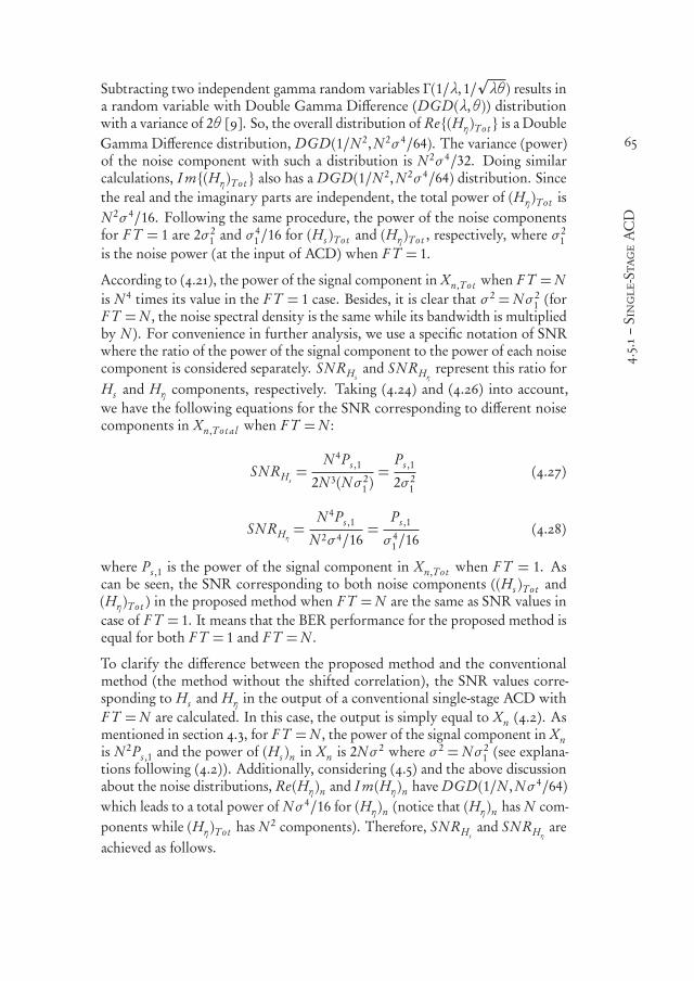
550999-L-bw-Siavash550999-L-bw-Siavash550999-L-bw-Siavash550999-L-bw-SiavashProcessed on: 23-11-2020Processed on: 23-11-2020Processed on: 23-11-2020Processed on: 23-11-2020 PDF page: 87PDF page: 87PDF page: 87PDF page: 87
65
4.5.1–Single-StageACD
Subtracting two independent gamma random variables Γ (1/λ, 1/pλθ) results in
a random variable with Double Gamma Difference (DGD(λ,θ)) distributionwith a variance of 2θ [9]. So, the overall distribution of Re(Hη)T ot is a DoubleGamma Difference distribution, DGD(1/N 2,N 2σ4/64). The variance (power)of the noise component with such a distribution is N 2σ4/32. Doing similarcalculations, I m(Hη)T ot also has a DGD(1/N 2,N 2σ4/64) distribution. Sincethe real and the imaginary parts are independent, the total power of (Hη)T ot isN 2σ4/16. Following the same procedure, the power of the noise componentsfor F T = 1 are 2σ2
1 and σ41/16 for (Hs )T ot and (Hη)T ot , respectively, where σ2
1is the noise power (at the input of ACD) when F T = 1.
According to (4.21), the power of the signal component in Xn,T ot when F T =Nis N 4 times its value in the F T = 1 case. Besides, it is clear that σ2 =Nσ2
1 (forF T =N , the noise spectral density is the same while its bandwidth is multipliedby N ). For convenience in further analysis, we use a specific notation of SNRwhere the ratio of the power of the signal component to the power of each noisecomponent is considered separately. SN RHs
and SN RHηrepresent this ratio for
Hs and Hη components, respectively. Taking (4.24) and (4.26) into account,we have the following equations for the SNR corresponding to different noisecomponents in Xn,T ot al when F T =N :
SN RHs=
N 4Ps ,1
2N 3(Nσ21 )=
Ps ,1
2σ21
(4.27)
SN RHη=
N 4Ps ,1
N 2σ4/16=
Ps ,1
σ41/16
(4.28)
where Ps ,1 is the power of the signal component in Xn,T ot when F T = 1. Ascan be seen, the SNR corresponding to both noise components ((Hs )T ot and(Hη)T ot ) in the proposed method when F T =N are the same as SNR values incase of F T = 1. It means that the BER performance for the proposed method isequal for both F T = 1 and F T =N .
To clarify the difference between the proposed method and the conventionalmethod (the method without the shifted correlation), the SNR values corre-sponding to Hs and Hη in the output of a conventional single-stage ACD withF T =N are calculated. In this case, the output is simply equal to Xn (4.2). Asmentioned in section 4.3, for F T =N , the power of the signal component in Xnis N 2Ps ,1 and the power of (Hs )n in Xn is 2Nσ2 where σ2 = Nσ2
1 (see explana-tions following (4.2)). Additionally, considering (4.5) and the above discussionabout the noise distributions, Re(Hη)n and I m(Hη)n have DGD(1/N ,Nσ4/64)which leads to a total power of Nσ4/16 for (Hη)n (notice that (Hη)n has N com-ponents while (Hη)T ot has N 2 components). Therefore, SN RHs
and SN RHηare
achieved as follows.

550999-L-bw-Siavash550999-L-bw-Siavash550999-L-bw-Siavash550999-L-bw-SiavashProcessed on: 23-11-2020Processed on: 23-11-2020Processed on: 23-11-2020Processed on: 23-11-2020 PDF page: 88PDF page: 88PDF page: 88PDF page: 88
66
Chapter4–ShiftedCorrelationDemodulatorforDDPSK
SN RHs=
N 2Ps ,1
2N (Nσ21 )=
Ps ,1
2σ21
(4.29)
SN RHη=
N 2Ps ,1
Nσ4/16=
Ps ,1
Nσ41/16
(4.30)
As shown by (4.30), the ratio of the signal power to the power of (Hη)T ot for theproposed method (see (4.28)) is N times its ratio for the conventional single-stageACD with only one path, whereas, as clarified by (4.27) and (4.29) this ratiofor (Hs )T ot is the same for the proposed method as for the conventional method.In the proposed method, although the Hη components are uncorrelated, theindividual terms in Hs are correlated. As can be seen in (4.29), even for theconventional ACD, SN RHs
is equal for both F T = 1 and F T = N . In otherwords, Hη (and not Hs ) is responsible for the difference in BER performancefor various F T values and the proposed method removes the effect of Hη. Thisconfirms our claim in the previous section.
4.5.2 Two-Stage ACD
The output of each path in the proposed demodulator (d R(L)n, p in Figure 4.4)
is composed of different components including signal-by-signal, signal-by-Hs ,signal-by-Hη, Hs -by-Hη and Hη-by-Hη. For large SNR, the terms including mul-tiplication of noise components resulting from the first stage (Hs -by-Hη andHη-by-Hη ) are negligible; thus, d R
n, p and d Ln, p can be approximated as follows:
d R(L)n, p ≈ SR(L)
n, p SR(L)n−1, p
+SR(L)n, p ((Hs )
R(L)n−1, p )
∗+(SR(L)n−1, p )
∗(Hs )R(L)n, p
+SR(L)n, p ((Hη)
R(L)n−1, p )
∗+(SR(L)n−1, p )
∗(Hη)R(L)n, p (4.31)
where SR(L)n, p , (Hs )
R(L)n, p and (Hη)
R(L)n, p are signal, signal-by-noise and nois-by-noise
components of X R(L)n, p , respectively. As shown before, the proposed method does
not affect SN RHs, so only the effect of noise components with Hη (the third line
in (4.31)) is analyzed here.
According to (4.16), the proposed method detects the transmitted symbol basedon dn,T ot al which is the sum of dn and d R(L)
n, p for all p. The rest of the mathemat-ical calculations focus on the sum of SR(L)
n, p ((Hη)R(L)n−1, p )
∗ components in dn,T ot al
for different values of p (in the remainder referred to as S ×H ∗η ) and the same
can be derived for (SR(L)n−1, p )
∗(Hη)R(L)n, p . Since SR(L)
n, p = (N − p)sn s∗n−1∆= (N − p)zn ,

550999-L-bw-Siavash550999-L-bw-Siavash550999-L-bw-Siavash550999-L-bw-SiavashProcessed on: 23-11-2020Processed on: 23-11-2020Processed on: 23-11-2020Processed on: 23-11-2020 PDF page: 89PDF page: 89PDF page: 89PDF page: 89
67
4.5.2–Two-StageACD
the corresponding noise component in the demodulator output is:
S ×H ∗η = N zn(Hη)n +N−1∑
p=1
zn(N − p)((Hη)Rn, p )∗
+N−1∑
p=1
zn(N − p)((Hη)Ln, p )∗ (4.32)
Since all ηk ,nη∗i ,n−1 are independent random variables, (Hη)n and ((Hη)
R(L)n, p )∗
are complex random variables (DGD distribution for real and imaginary parts)with a variance of Nσ4/16 and (N − p)σ4/16, respectively (this is derived usingthe same process as in the previous section). As the signal component, zn , isa constant complex number, where zn z∗n = 1 (4.1), the variance of each terminside the sum over p in (4.32) would be (N − p)3σ4/16 and the variance of thefirst term on (4.32) is N 3σ4/16. All terms in the right hand side of (4.32) areindependent, so the total power is:
P(S×H ∗η )=σ4
16(N 3+
N−1∑
p=1
2(N − p)3) =N 2(N 2+ 1)
2σ4
16(4.33)
When F T = N , the signal component S(dn )T ot ,F T=N in dn,T ot which is the finaloutput of the demodulator (see (4.18)) equals to:
S(dn )T ot ,F T=N = Sn +N−1∑
p=1
SRn, p (S
Rn−1, p )
∗+N−1∑
p=1
SLn, p (S
Ln−1, p )
∗
= zn z∗n−1(N2+ 2
N−1∑
p=1
(N − p)2)
= zn z∗n−1(N (2N 2+ 1)
3) (4.34)
To achieve the last line of (4.34), Faulhaber’s formula for the sum of squaresof N first positive integers (1,2, ...,N ) can be used. When F T = 1 the signalcomponent is zn z∗n−1 so, according to (4.34), the power of the signal componentin the output of the proposed demodulator, when F T =N , is N 2(2N 2+ 1)2/9times the power of the signal component for F T = 1, Ps ,1. Thus, from (4.33)SN RS×H ∗η ,F T=N is:
SN RS×H ∗η ,F T=N =329
N 2(2N 2+ 1)2Ps ,1
N 2(N 2+ 1)σ4(4.35)
Based on (4.35), SN RS×H ∗η ,F T=1 (N = 1) can be derived.

550999-L-bw-Siavash550999-L-bw-Siavash550999-L-bw-Siavash550999-L-bw-SiavashProcessed on: 23-11-2020Processed on: 23-11-2020Processed on: 23-11-2020Processed on: 23-11-2020 PDF page: 90PDF page: 90PDF page: 90PDF page: 90
68
Chapter4–ShiftedCorrelationDemodulatorforDDPSK
SN RS×H ∗η ,F T=1 = 16Ps ,1
σ41
(4.36)
Considering that σ2 = Nσ21 and from (4.35) and (4.36), the ratio of the SNR
corresponding to the S × H ∗η component for F T = N and F T = 1 can becalculated as:
SN RS×H ∗η ,F T=N
SN RS×H ∗η ,F T=1=
8N 4+ 8N 2+ 29N 4+ 9N 2
(4.37)
The limit of the above ratio when N →∞ is 0.89 (only 11% loss compared toF T = 1) while for N = 2 this ratio is 0.9. Using only Xn as the output and similarto (4.30), the same ratio (as in (4.37)) for conventional DDPSK will be equal to1/N . Although SN RS×H ∗η ,F T=N for the proposed method is not equal to the caseof F T = 1, it is much higher than its value for the conventional method. Thishigher SNR leads to an improved BER performance for the proposed methodcompared to the conventional DDPSK. Besides, the minimum SNR, related tothe discussed noise components for the proposed demodulator, equals 0.89 timesits value for F T = 1 even in case of arbitrarily large N .
4.6 Simulation Results and BER Performance Analysis
To demonstrate the performance of the multipath ACD demodulator and toverify the mathematical calculations presented in the previous section, the BERcurves for DPSK and DDPSK are presented in this section. Figure 4.5 andFigure 4.6 show BER curves for Binary DPSK (DBPSK) and Binary DDPSK(DDBPSK), respectively. Similar to [94], BER curves are presented for differentvalues of F T including F T = 1,8,16. For comparison, the BER curves for theconventional demodulator are also demonstrated.
As can be seen in Figure 4.5, for F T = 1 in a conventional ACD, the BERperformance is the same as a non-coherent DBPSK; whereas, for F T = 8 andF T = 16 the performance degrades considerably. As can be seen, the Eb/N0for a BER= 0.1% increases by 2dB and 3dB for F T = 8 and F T = 16, respec-tively. Using the proposed structure for a single-stage ACD, the BER curves forboth F T values exactly match the BER curve for F T = 1 which matches theconclusion of our discussion in the previous section.
For DDBPSK, the proposed method is applied to T − 2T DDBPSK and theresults are shown for F T = 1,8,16 in Figure 4.6. The proposedmethod is appliedto the T − 2T DDBPSK by replacing N with 2N in the delays of the first stageof the proposed demodulator (see Figure 4.4). To demonstrate the improvementachieved by the proposed method in case of DDBPSK, the BER curves of aconventional demodulator for F T = 8,16 are illustrated. It can be seen that forF T = 16 the proposed method saves Eb/N0 required for BER= 0.1% by almost
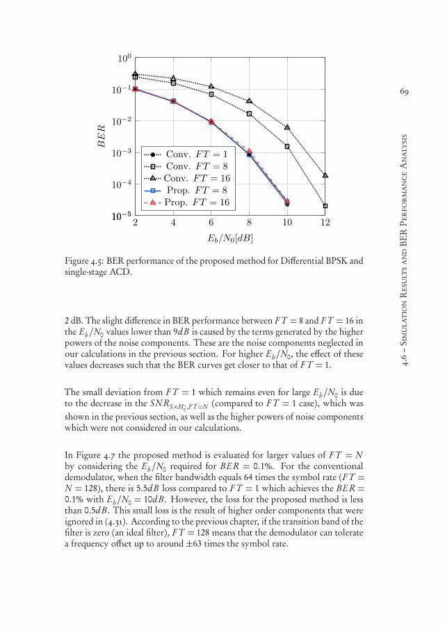
550999-L-bw-Siavash550999-L-bw-Siavash550999-L-bw-Siavash550999-L-bw-SiavashProcessed on: 23-11-2020Processed on: 23-11-2020Processed on: 23-11-2020Processed on: 23-11-2020 PDF page: 91PDF page: 91PDF page: 91PDF page: 91
69
4.6–SimulationResultsandBERPerformanceAnalysis
2 4 6 8 10 1210−510−5
10−4
10−3
10−2
10−1
100
Eb/N0[dB]
BER
Conv. FT = 1Conv. FT = 8Conv. FT = 16Prop. FT = 8Prop. FT = 16
Figure 4.5: BER performance of the proposed method for Differential BPSK andsingle-stage ACD.
2 dB. The slight difference in BER performance between F T = 8 and F T = 16 inthe Eb/N0 values lower than 9dB is caused by the terms generated by the higherpowers of the noise components. These are the noise components neglected inour calculations in the previous section. For higher Eb/N0, the effect of thesevalues decreases such that the BER curves get closer to that of F T = 1.
The small deviation from F T = 1 which remains even for large Eb/N0 is dueto the decrease in the SN RS×H ∗η ,F T=N (compared to F T = 1 case), which wasshown in the previous section, as well as the higher powers of noise componentswhich were not considered in our calculations.
In Figure 4.7 the proposed method is evaluated for larger values of F T = Nby considering the Eb/N0 required for BER = 0.1%. For the conventionaldemodulator, when the filter bandwidth equals 64 times the symbol rate (F T =N = 128), there is 5.5dB loss compared to F T = 1 which achieves the BER =0.1% with Eb/N0 = 10dB . However, the loss for the proposed method is lessthan 0.5dB . This small loss is the result of higher order components that wereignored in (4.31). According to the previous chapter, if the transition band of thefilter is zero (an ideal filter), F T = 128 means that the demodulator can toleratea frequency offset up to around ±63 times the symbol rate.

550999-L-bw-Siavash550999-L-bw-Siavash550999-L-bw-Siavash550999-L-bw-SiavashProcessed on: 23-11-2020Processed on: 23-11-2020Processed on: 23-11-2020Processed on: 23-11-2020 PDF page: 92PDF page: 92PDF page: 92PDF page: 92
70
Chapter4–ShiftedCorrelationDemodulatorforDDPSK
2 4 6 8 10 1210−510−5
10−4
10−3
10−2
10−1
100
Eb/N0[dB]
BER
Conv. FT = 1Conv. FT = 8Conv. FT = 16Prop. FT = 8Prop. FT = 16
Figure 4.6: BER performance of the proposed method for Double DifferentialBPSK and two-stage ACD
20 40 60 80 100 12010
11
12
13
14
15
16
N
Eb/N
0forBER
=0.1%
ConventionalProposed
Figure 4.7: The Eb/N0 required for a BER= 0.1% when N increases

550999-L-bw-Siavash550999-L-bw-Siavash550999-L-bw-Siavash550999-L-bw-SiavashProcessed on: 23-11-2020Processed on: 23-11-2020Processed on: 23-11-2020Processed on: 23-11-2020 PDF page: 93PDF page: 93PDF page: 93PDF page: 93
71
4.7–ComplexityandPerformanceTrade-off
2 4 6 8 10 1210−510−5
10−4
10−3
10−2
10−1
100
Eb/N0[dB]
BER P=0
P=1P=2P=4P=8P=15FT = 1
Figure 4.8: The BER performance of the proposed demodulator for differentvalues of P where p = 1, ..., P and F T = 16
4.7 Complexity and Performance Trade-off
According to the results presented so far, the BER performance of the proposeddemodulator remains almost constant when the filter bandwidth increases. Ob-viously, this improvement is achieved at the cost of increased digital complexity.Inspecting the structure of the proposed demodulator, one may recognize a trade-off between the complexity and the BER performance. When all paths are usedi.e. p = 1, ...,N − 1, the BER performance is almost the same as F T = 1. Never-theless, all paths do not contribute equally to the performance improvement.
When p increases, the number of samples used for calculating X R(L)n, p decreases
due to shifting symbols relative to each other (see Figure 4.2). It means that theX R(L)
n, p for higher values of p generates fewer uncorrelated replicas of the noise-by-noise component. If a compromise for the BER performance is acceptable,fewer paths can be used. Each path adds N − p complex multiplications in thefirst stage and one complex multiplication in the second stage.
To see this effect, the BER curves in case of F T = 16 and F T = 64 for differentvalues of P (where p = 1, ..., P ) are shown in Figure 4.8 and 4.9, respectively.
These figures show that only adding one path (in each direction) contributes toalmost half of the saving in the Eb/N0 required for BER= 0.1%. It is interestingthat for P = N/2 the BER curve is hardly distinguishable from the best case(P = N − 1). However, the complexity for P = N/2 is 75% of the complexity
550999-L-bw-Siavash550999-L-bw-Siavash550999-L-bw-Siavash550999-L-bw-SiavashProcessed on: 23-11-2020Processed on: 23-11-2020Processed on: 23-11-2020Processed on: 23-11-2020 PDF page: 94PDF page: 94PDF page: 94PDF page: 94
72
Chapter4–ShiftedCorrelationDemodulatorforDDPSK
4 6 8 10 12 14 1610−510−5
10−4
10−3
10−2
10−1
100
Eb/N0[dB]
BER P = 0
P = 1P = 2P = 16P = 32P = 65FT = 1
Figure 4.9: The BER performance of the proposed demodulator for differentvalues of P where p = 1, ..., Pand F T = 64
0 2 4 6 8 10 12 14 16 1810
11
12
13
14
15
Number of CM normalized to N + 1
Eb/N
0forBER
=0.1%
N = 16
0 10 20 30 40 50 60 7010
11
12
13
14
15
Number of CM normalized to N + 1
Eb/N
0forBER
=0.1%
N = 64
Figure 4.10: Performance and complexity trade-off for N = 16 and N = 64(CM=Complex Multiplication).
of the proposed demodulator with P = N − 1. To clarify the complexity andperformance trade-off, the Eb/N0 required for BER= 0.1% versus complexityis illustrated in Figure 4.10 for F T = 16 and F T = 64. The complexity iscalculated in terms of the number of complex multiplications and is normalizedto the complexity of the conventional demodulator (equivalent to P = 0). Inboth cases for a complexity around 50% of the complexity of P = N − 1 theEb/N0 required for BER= 0.1% is only around 0.5 dB higher than its value forF T = 1 which is 10 dB (see Figure 4.8 and Figure 4.9).

550999-L-bw-Siavash550999-L-bw-Siavash550999-L-bw-Siavash550999-L-bw-SiavashProcessed on: 23-11-2020Processed on: 23-11-2020Processed on: 23-11-2020Processed on: 23-11-2020 PDF page: 95PDF page: 95PDF page: 95PDF page: 95
73
4.8–Conclusion
4.8 Conclusion
The BER performance of the autocorrelation demodulator (ACD) for DDPSKin the presence of a large frequency offset was considered. The bandwidth of thefilter before the demodulator should be selected according to the target range forthe frequency offset tolerance. AlthoughDDPSK is able to tolerate frequency off-set, the wide filter increases the noise bandwidth at the input of the demodulatorwhich leads to BER performance degradation. The proposed demodulator addsadditional paths to the conventional DDPSK demodulator and the sum of de-modulated signals in these paths is sent to the detector. As shown in this chapter,the proposed method increases SNR at the input of the detector and compensatesfor SNR loss resulting from the wider filter. Therefore, the BER performanceremains unchanged for all values of the filter bandwidth. The simulation resultsrevealed that the proposed method leads to more than 2 dB improvement in theBER performance in case the bandwidth of the filter is 8 times the symbol rate(F T = 16). For a wider filter i.e. a wider range of frequency offset tolerance, thisgain increases. The complexity of the proposed method was also investigatedand the trade-off between the BER performance and complexity was presented.

550999-L-bw-Siavash550999-L-bw-Siavash550999-L-bw-Siavash550999-L-bw-SiavashProcessed on: 23-11-2020Processed on: 23-11-2020Processed on: 23-11-2020Processed on: 23-11-2020 PDF page: 96PDF page: 96PDF page: 96PDF page: 96
74

550999-L-bw-Siavash550999-L-bw-Siavash550999-L-bw-Siavash550999-L-bw-SiavashProcessed on: 23-11-2020Processed on: 23-11-2020Processed on: 23-11-2020Processed on: 23-11-2020 PDF page: 97PDF page: 97PDF page: 97PDF page: 97
755Low Complexity Implementation
of the FSK Demodulator
Abstract – The DFT-based demodulator for BFSK has been introduced asan offset tolerant demodulator capable of tolerating a large Carrier FrequencyOffset (CFO). However, it was shown in Chapter 3 that its limitation in caseof a large frequency offset is its complexity. The main source of complexity, iscalculating the DFT of a window which slides over the preamble. In this chap-ter, the complexity is alleviated by considering the window synchronizationalgorithm and its implementation together. First, a new window synchro-nization algorithm is proposed which is designed such that an efficient classof the implementations of the Sliding DFT (SDFT), called Single Bin SDFT(SB-SDFT) in this chapter, can be used. Moreover, a stable implementationof the SB-SDFT is designed to enable zero-padding which is required by thedemodulator. The complexity of the proposed algorithm implemented usingthe SB-SDFT, scales more efficiently compared to the conventional algorithmwhen the range of tolerable CFO increases. Using the proposed method, fora CFO tolerance in the order of 14.5 times the symbol rate (±1.45 kHz for asymbol rate equal to 100 Hz), the number of complex operations is reduced bymore than 85% (and memory by 90%) compared to the conventional method.
5.1 Introduction
A DFT-based demodulator for BFSK was introduced in Chapter 3. As discussedearlier, the prominent drawback is that a complex synchronization scheme isused to properly select the samples of a symbol for which the DFT is calculated.The computational complexity of the synchronization stems from the DFTcalculation for a window which is sliding over the synchronization preamble.Various methods have been proposed for efficient implementation of the DFT
This chapter is based on [S:2] and [S:6].

550999-L-bw-Siavash550999-L-bw-Siavash550999-L-bw-Siavash550999-L-bw-SiavashProcessed on: 23-11-2020Processed on: 23-11-2020Processed on: 23-11-2020Processed on: 23-11-2020 PDF page: 98PDF page: 98PDF page: 98PDF page: 98
76
Chapter5–LowComplexityImplementationoftheFSKDemodulator
with a sliding window [20, 24, 26, 29–31, 42, 48, 53, 72, 73, 78–80, 85, 100, 101].Investigating these techniques, which are explicated in section 5.3, reveals thatthe most efficient design can be obtained if the synchronization algorithm onlyrequires a subset of the DFT bins.
In light of these facts, a low complexity synchronization algorithm is proposedin this chapter and a modified stable Single-Bin Sliding DFT (SB-SDFT) calcu-lator is introduced for its implementation. Furthermore, the complexity of theproposed synchronization algorithm implemented using the SB-SDFT structureis analyzed and compared to an efficient implementation of the conventionalalgorithm.
First a brief review of the DFT-based demodulator and the conventional synchro-nization algorithm from Chapter 3 are explained in the next section. Section 5.3looks into related work on the efficient implementation of a sliding DFT whilejointly motivating the design of the proposed synchronization algorithm and theproposed SB-SDFT. Subsequently, the proposed synchronization algorithm ispresented in Section 5.4. Next, section 5.5 elaborates on the proposed SB-SDFTand derives its stabilized version. The complexity analysis follows in Section 5.6to obtain expressions for the number of operations and memory use. Numericalresults and discussions are included in section 5.7. Finally, section 5.8 concludesthis chapter.
5.2 A Brief Review of the Problem
5.2.1 Demodulator and Synchronization Algorithm
In this section, the DFT-based demodulator and the window synchronizationalgorithm from Chapter 3 are (briefly) explained again to ease the reading. Theblock diagram of the DFT based demodulator is shown in Figure 5.1 (this is thesame block diagram from Chapter 3 and is repeated for easier reference). Signalsamples pass through a low-pass filter prior to the demodulator. To toleratelarge Carrier Frequency Offset (CFO), the low-pass filter might be much widerthan the signal bandwidth. Moreover, complying with the Nyquist criterionnecessitates a higher sampling frequency. Assuming an ideal brick-wall filter, thesignal samples just before the demodulator are as follows.
rm[n] = exp( j (2π( fm + fO )nTs +θ)), (5.1)
where rm[n] is the n t h sample (n = 0, ...,N − 1) of the m t h symbol; fm istransmitted frequency during m t h symbol which is either f0 or f1; θ is thephase offset, fO is the frequency offset and Ts is the sampling period. After thefilter, a proper set of samples (all belonging to the same symbol) is selected by arectangular window, padded with zeros and sent to the DFT calculation block

550999-L-bw-Siavash550999-L-bw-Siavash550999-L-bw-Siavash550999-L-bw-SiavashProcessed on: 23-11-2020Processed on: 23-11-2020Processed on: 23-11-2020Processed on: 23-11-2020 PDF page: 99PDF page: 99PDF page: 99PDF page: 99
77
5.2.1–DemodulatorandSynchronizationAlgorithm
DFT Calc.
Window &Zero-Padding Detection
Synchronization
LPF
Timing
Figure 5.1: Block diagram of the DFT-based demodulator from Chapter 3
to achieve the following.
Xk ,m =N I−1∑
n=0
xIm[n]exp(− j
2πknN I
) (5.2)
where, Xk ,m is the k t h bin of the DFT calculated for m t h symbol. I is thezero-padding factor which means that N samples of the signal are padded byN (I−1) zeros to achieve a zero-padded sequence xI
m with length N I as the inputof the DFT. Finally, the decision for each symbol of BFSK is made based onthe magnitudes of Xk ,m . Zero-padding is used to improve the bin resolutionof the DFT as explained in Chapter 3. The frequency separation of the BFSKmodulation is assumed to be equal to the symbol rate ( f1 = +1/2T and f0 =−1/2T in (5.1)).
Two phases can be distinguished in the demodulator operation. First, the win-dow must be aligned to the received symbols; otherwise, frequency componentsof the adjacent symbols introduce inter-symbol interference. This window align-ment is done during the synchronization phase. Furthermore, theDFT frequencybins corresponding to the frequency of symbol one (k1 ) and zero (k0 ) of theBFSK modulation are determined in this phase [89]. In the detection phase, theDFT is calculated for the samples of each symbol. For each symbol the decisionis made by comparing the magnitude of the DFT bins k1 and k0.
The synchronization algorithm discussed in Chapter 3 has been introduced byHara et al. [44] and, in the rest of this chapter, is referred to as Hara synchro-nization or the conventional synchronization algorithm. It uses a preamble ofalternating ones and zeros. The number of symbols in the preamble is denotedby L. For each symbol, windows with different delay values, between 0 andN − 1, are considered. Only one of these windows is fully aligned with onesymbol and others include samples of two consecutive symbols. The DFT iscalculated for each window. Figure 5.2 illustrates three symbols of the preambleand the windows in case of four samples per symbol (this is the same blockdiagram from Chapter 3 and is repeated for easier reference). It also shows howthe spectrum varies for different delays. The symbols of preamble are calledEven and Odd depending on their index m = 1, ...L. All DFT magnitudes cor-

550999-L-bw-Siavash550999-L-bw-Siavash550999-L-bw-Siavash550999-L-bw-SiavashProcessed on: 23-11-2020Processed on: 23-11-2020Processed on: 23-11-2020Processed on: 23-11-2020 PDF page: 100PDF page: 100PDF page: 100PDF page: 100
78
Chapter5–LowComplexityImplementationoftheFSKDemodulator
responding to Odd symbols (Even symbols) in the preamble are added togetherto achieve the following.
SOi (k) =
L/2∑
n=1
X 2n−1k ,i (5.3)
SEi (k) =
L/2∑
n=1
X 2nk ,i (5.4)
where i = 0, ...,N − 1 is the window delay. This is visualized in Figure 5.2.The double-headed arrows denote windows. Each row of arrows correspondto a certain delay value as shown in the figure. Solid (dotted) arrows show thewindows for an Odd (Even) symbol with different delay values. In fact, (5.3)and (5.4) calculate the sum of the DFT magnitudes for solid windows and thesum of those for dotted windows, respectively.
To synchronize the window, the Hara algorithm finds the delay value for whichRi in the following equation is maximized.
Ri = [SEi (k
Ei )− SE
i (kOi )]+ [S
Oi (k
Oi )− SO
i (kEi )], (5.5)
where kEi and kO
i are the bins with maximum magnitude in SEi and SO
i , respec-tively. Finding the maximum of (3.9) is simply finding the delay value whichmaximizes the difference shown by D in Figure 5.2. When the delay value isfound, the k1 and k0 can be achieved from kO
i and kEi , respectively.
5.2.2 A Quick Look at Complexity
The number of complex multiplications (CM) and complex additions (CA) re-quired for the synchronization and detection phases are listed in Table 5.1 fora system with N = I = 8 and L = 16 (the same as Chapter 3). The detailedcalculations for complexity can be found in Chapter 3. Synchronization is doneonce in a packet so its complexity must be divided by the number of symbols in apacket to achieve the complexity per symbol. According to Table 5.1, the packetlength for which detection complexity per symbol exceeds synchronization com-plexity is more than 1400 symbols. This is much larger than the packet lengthin UNB communications (in order of 200 symbols). Moreover, the operationsrequired for synchronization are done in a shorter period of time compared tothe detection phase which leads to high instantaneous power consumption as aconsequence of higher clock frequencies. This makes it unsuitable for applica-tions where maximum instantaneous power is limited. Thus, the complexity ofthe synchronization algorithm is always dominant and needs to be alleviated.
As mentioned before in the Hara synchronization algorithm, the DFT is calcu-lated for a window which slides over the preamble. This plays the paramountrole in the complexity of the demodulator but can be implemented efficiently

550999-L-bw-Siavash550999-L-bw-Siavash550999-L-bw-Siavash550999-L-bw-SiavashProcessed on: 23-11-2020Processed on: 23-11-2020Processed on: 23-11-2020Processed on: 23-11-2020 PDF page: 101PDF page: 101PDF page: 101PDF page: 101
79
5.2.2–A
QuickLookatComplexity
DDelay=0
Delay=2
f0 f1
f0 f1
D
Delay=1
Delay=3
f0 f1
f0 f1
D
D
Delay=0
Delay=1
Delay=2
Delay=3
Odd Symbols ( ) Even Symbols ( )
Figure 5.2: The first three symbols of a preamble, the windows of different delayvalues for the first two symbols and an example of spectrum variation when thereare 4 samples per symbol. Solid and dotted lines show windows and spectra ofodd and even symbols, respectively.
Table 5.1: Complexity of different phases in the demodulator for N = I = 8 andL = 16. CM and CA stand for complex multiplication and complex addition,respectively.
Demodulator Phase CA CM
Detection (/Symbol) 14 16
Synchronization (/Packet) 46080 23040
using Sliding DFT algorithms. The next section elaborates on the efficient im-plementation of the Sliding DFT reviewing related literature.

550999-L-bw-Siavash550999-L-bw-Siavash550999-L-bw-Siavash550999-L-bw-SiavashProcessed on: 23-11-2020Processed on: 23-11-2020Processed on: 23-11-2020Processed on: 23-11-2020 PDF page: 102PDF page: 102PDF page: 102PDF page: 102
80
Chapter5–LowComplexityImplementationoftheFSKDemodulator
5.3 Related Work on the Sliding DFT (SDFT)
Calculating the DFT for a window which is sliding over a sequence is calledSliding DFT (SDFT). As a computationally intensive block, many researchershave investigated the efficient implementation of the SDFT. In case of a slidingwindow, only one sample (or a few samples) is (are) different between the currentset of input samples of the DFT and the previous set. Exploiting this property,various methods have been proposed [20, 24, 26, 29–31, 42, 48, 53, 72, 73, 78–80, 85, 100, 101]. By reusing calculations done for each window, the DFT ofthe next window can be calculated in a more efficient way. For a better under-standing, we categorize the methods into two general groups. The first group,Complete SDFT (C-SDFT), includes algorithms that calculate all the DFT binsfor each window in a single structure; whereas, the second category, Single-Bin SDFT (SB-SDFT), covers algorithms which derive only a single bin of theDFT. These categories are explained in the next two subsections. Althoughthe final design in this work belongs to the SB-SDFT category, review of theC-SDFT methods is necessary. It helps us to derive an efficient implementationof the Hara synchronization algorithm (the algorithm explained in the previ-ous section) which is used as a benchmark for complexity comparison. In thelast subsection, the conclusions that can be drawn from literature are pointedout. This subsection also describes how this insight provokes the design of theproposed algorithm and the proposed SB-SDFT.
5.3.1 Complete SDFT (C-SDFT)
One of the initial examples of an SDFT has been introduced in [20, 30, 31]. Basedon the conventional Decimation-in-Time FFT structure and storing calculatedintermediate values, this method decreases the complexity of the FFT calcula-tion for the new coming sample from O (N log2 N ) in the FFT to O (N ) [30].However, it increases the required memory as it needs to store all the intermedi-ate values. In our complexity analysis in section 5.6, this structure is consideredfor the implementation of the Hara synchronization algorithm; therefore, it isworth to explain it in more detail. Figure 5.3 shows the FFT structure used in[30] where the old window samples are shown in a dashed box (in grey) and thewhite circles show butterflies of the FFT. Samples x(n− 16) to x(n− 1) (insidethe dashed box) belong to the (n − 1)t h window. When sample x(n) is added,samples x(n−15) to x(n) are included in the n t h window and the FFT for themmust be calculated. It can be seen that all required butterflies except for thehighlighted ones can be derived from butterfly outputs of the (n− 1)t h window.In other words, when the window slides one sample, only one butterfly fromeach group of butterflies using the same twiddle factor (those in one dashed oval)needs to be calculated. For an N -point FFT, only N − 1 butterflies must becalculated when the window slides for one sample. This method is one of themost efficient ways to calculate the C-SDFT and is called Sliding FFT (SFFT)hereafter.

550999-L-bw-Siavash550999-L-bw-Siavash550999-L-bw-Siavash550999-L-bw-SiavashProcessed on: 23-11-2020Processed on: 23-11-2020Processed on: 23-11-2020Processed on: 23-11-2020 PDF page: 103PDF page: 103PDF page: 103PDF page: 103
81
5.3.1–CompleteSDFT(C-SDFT)
X(0)
X(1)
X(15)
X(2)
X(3)
X(4)
X(5)
X(6)
X(7)
X(8)
X(9)
X(10)
X(11)
X(12)
X(13)
X(14)
x(n)
x(n-1)
x(n-2)
x(n-3)
x(n-4)
x(n-5)
x(n-6)
x(n-7)
x(n-8)
x(n-9)
x(n-10)
x(n-11)
x(n-12)
x(n-13)
x(n-14)
x(n-15)
x(n-1)
x(n-2)
x(n-3)
x(n-4)
x(n-5)
x(n-6)
x(n-7)
x(n-8)
x(n-9)
x(n-10)
x(n-11)
x(n-12)
x(n-13)
x(n-14)
x(n-15)
x(n-16)
x(n)
x(n-16)
Figure 5.3: The Sliding FFT structure introduced by [30]. The dashed box inthe left includes the samples belonging to the old window. When the windowslides one sample, the samples in the solid box will be new inputs to the FFT.The butterflies enclose in each dashed oval are called a group of butterfly. Eachgroup uses the same twiddle factor for calculations.
Interpreting the FFT structure as a prism, Wang et al. [100] proposed a methodto calculate the SDFT. Although its complexity is more than that of the SFFTin [30], it can be implemented in parallel for faster calculation [101] which is notnecessary in our target application as it involves very low data rates. Rewritingthe sliding DFT definition and using time shift properties, Montoya et al. haveproposed a sliding DFT method with almost 50% reduction in the number ofcomplex multiplications compared to the SFFT [73]. This idea is also extendedto a Radix-4 decomposition in [72] which achieves even more savings at the costof limiting the DFT points to a power of four. Despite the complexity reductionachieved in [72, 73], these cannot be used when zero-padding is involved whichis the case in our target application. A guaranteed stable recursive algorithm forcalculation of all bins is proposed in [78] which is based on a single bin recursivestructure from the same author in [80]. This method is only applicable in ahopping scenario where each window hops N/4 samples (N is the DFT size).
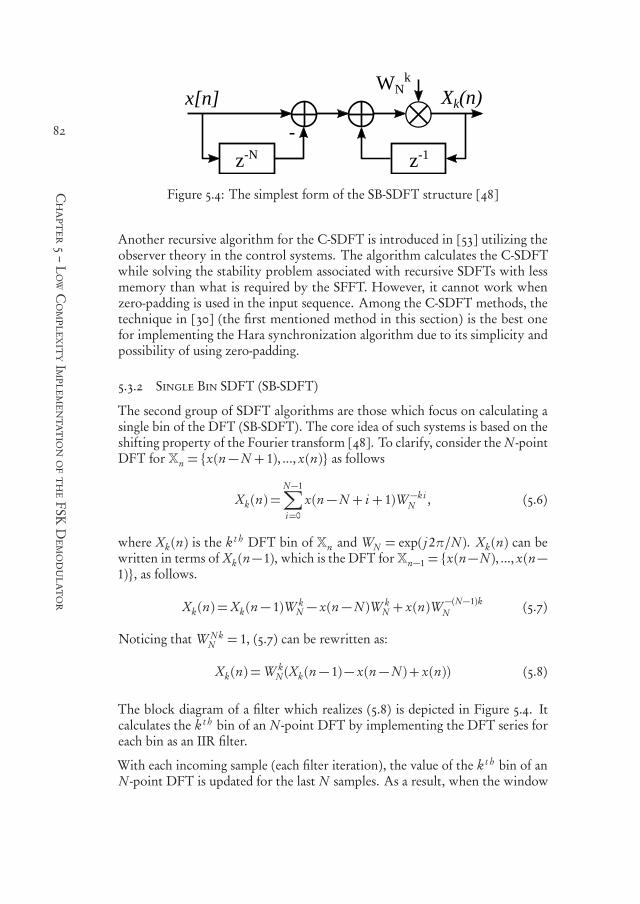
550999-L-bw-Siavash550999-L-bw-Siavash550999-L-bw-Siavash550999-L-bw-SiavashProcessed on: 23-11-2020Processed on: 23-11-2020Processed on: 23-11-2020Processed on: 23-11-2020 PDF page: 104PDF page: 104PDF page: 104PDF page: 104
82
Chapter5–LowComplexityImplementationoftheFSKDemodulator
z-N
WNk
-z-1
x[n] Xk(n)
Figure 5.4: The simplest form of the SB-SDFT structure [48]
Another recursive algorithm for the C-SDFT is introduced in [53] utilizing theobserver theory in the control systems. The algorithm calculates the C-SDFTwhile solving the stability problem associated with recursive SDFTs with lessmemory than what is required by the SFFT. However, it cannot work whenzero-padding is used in the input sequence. Among the C-SDFT methods, thetechnique in [30] (the first mentioned method in this section) is the best onefor implementing the Hara synchronization algorithm due to its simplicity andpossibility of using zero-padding.
5.3.2 Single Bin SDFT (SB-SDFT)
The second group of SDFT algorithms are those which focus on calculating asingle bin of the DFT (SB-SDFT). The core idea of such systems is based on theshifting property of the Fourier transform [48]. To clarify, consider the N -pointDFT for Xn = x(n−N + 1), ..., x(n) as follows
Xk (n) =N−1∑
i=0
x(n−N + i + 1)W −kiN , (5.6)
where Xk (n) is the k t h DFT bin of Xn and WN = exp( j 2π/N ). Xk (n) can bewritten in terms of Xk (n−1), which is the DFT for Xn−1 = x(n−N ), ..., x(n−1), as follows.
Xk (n) =Xk (n− 1)W kN − x(n−N )W k
N + x(n)W −(N−1)kN (5.7)
Noticing that W N kN = 1, (5.7) can be rewritten as:
Xk (n) =W kN (Xk (n− 1)− x(n−N )+ x(n)) (5.8)
The block diagram of a filter which realizes (5.8) is depicted in Figure 5.4. Itcalculates the k t h bin of an N -point DFT by implementing the DFT series foreach bin as an IIR filter.
With each incoming sample (each filter iteration), the value of the k t h bin of anN -point DFT is updated for the last N samples. As a result, when the window
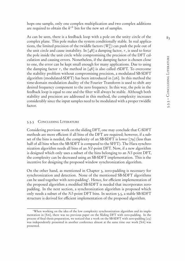
550999-L-bw-Siavash550999-L-bw-Siavash550999-L-bw-Siavash550999-L-bw-SiavashProcessed on: 23-11-2020Processed on: 23-11-2020Processed on: 23-11-2020Processed on: 23-11-2020 PDF page: 105PDF page: 105PDF page: 105PDF page: 105
83
5.3.3–ConcludingLiterature
hops one sample, only one complex multiplication and two complex additionsare required to obtain the k t h bin for the new set of samples.
As can be seen, there is a feedback loop with a pole on the unity circle of thecomplex plane. This pole makes the system conditionally stable. In real applica-tions, the limited precision of the twiddle factors (W k
N ) can push the pole out ofthe unit circle and cause instability. In [48] a damping factor, r , is used to forcethe pole inside the unit circle while compromising the precision of the DFT cal-culation and causing errors. Nonetheless, if the damping factor is chosen closeto one, the error can be kept small enough for many applications. Due to usingthe damping factor r , the method in [48] is also called rSDFT. To overcomethe stability problem without compromising precision, a modulated SB-SDFTalgorithm (modulated-SDFT) has been introduced in [26]. In this method thetime-domain modulation duality of the Fourier Transform is used to shift anydesired frequency component to the zero frequency. In this way, the pole in thefeedback loop is equal to one and the filter will always be stable. Although bothstability and precision are addressed in this method, the complexity increasesconsiderably since the input samples need to be modulated with a proper twiddlefactor.
5.3.3 Concluding Literature
Considering previous work on the sliding DFT, one may conclude that C-SDFTmethods are more efficient if all bins of the DFT are required; however, if a sub-set of the bins is needed, the complexity of an SB-SDFT is lower [79] (less thanhalf of all bins when the SB-SDFT is compared to the SFFT). The Hara synchro-nization algorithm needs all bins of an N I -point DFT. Now, if a new algorithmis designed which only uses a subset of the bins belonging to an N I -point DFT,the complexity can be decreased using an SB-SDFT implementation. This is theincentive for designing the proposed window synchronization algorithm.
On the other hand, as mentioned in Chapter 3, zero-padding is necessary forsynchronization and detection. None of the mentioned SB-SDFT algorithmscan be used together with zero-padding1. Hence, for efficient implementation ofthe proposed algorithm a modified SB-SDFT is needed that incorporates zero-padding. In the next section, a synchronization algorithm is proposed whichonly needs a subset of the N I -point DFT bins. In section 5.5, a stable SB-SDFTstructure is derived for efficient implementation of the proposed algorithm.
1When working on the idea of the low complexity synchronization algorithm and its imple-mentation in [S:6], there was no previous paper on the Sliding DFT with zero-padding. In theprocess of final thesis preparation, we noticed that a work on the SB-SDFT with zero-padding [23]was independently presented in another conference almost at the same time our work [S:6] waspresented.

550999-L-bw-Siavash550999-L-bw-Siavash550999-L-bw-Siavash550999-L-bw-SiavashProcessed on: 23-11-2020Processed on: 23-11-2020Processed on: 23-11-2020Processed on: 23-11-2020 PDF page: 106PDF page: 106PDF page: 106PDF page: 106
84
Chapter5–LowComplexityImplementationoftheFSKDemodulator
BoI
Figure 5.5: The spectrum of the signal and the BoI
5.4 The Proposed Window Synchronization Algorithm
So far, it has been concluded that using only a subset of the bins of an N I -pointDFT for window synchronization reduces complexity compared to the Harasynchronization method. Before introducing the proposed synchronization al-gorithm, it is needed to check whether it is feasible to only rely on a subset ofbins for synchronization (without losing signal information). This is done in thefirst subsection where a set called Bins of Interest (BoI) is defined and the generalconcept of the proposed synchronization algorithm is introduced. Afterwards,the algorithm is described in detail.
5.4.1 Bins of Interest and the Proposed Synchronization Concept
In the presence of a large frequency offset (multiple times the symbol rate) afilter wider than (multiple times) the signal bandwidth before the demodulatoris needed to capture the signal. It means that the sampling frequency shouldbe higher than the actual information bearing bandwidth of the signal. Onthe other hand, using zero-padding increases the number of bins that must becalculated including those which are out of the signal bandwidth. As a result ofthis oversampling and zero-padding, only a small part of the spectrum calculatedby an N I -point DFT includes signal information. These bins of the spectrum arecalled Bins of Interest hereafter and BoI for each DFT is defined as the set whichincludes these bins. Since the signal information resides in the BoI, solely theBoI can already provide a correct synchronization without loss of information.The BoI is in the vicinity of the frequency offset in the baseband signal whichis called center frequency fc in the following ( fc = fO ). This is shown in Figure5.5 for a case where the sampling frequency is 8 times the symbol rate and azero-padding factor of 4 is used (32-point DFT). In Figure 5.5, the k0, k1 and kccorrespond to the frequencies f0, f1 and fc , respectively.
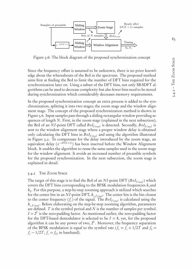
550999-L-bw-Siavash550999-L-bw-Siavash550999-L-bw-Siavash550999-L-bw-SiavashProcessed on: 23-11-2020Processed on: 23-11-2020Processed on: 23-11-2020Processed on: 23-11-2020 PDF page: 107PDF page: 107PDF page: 107PDF page: 107
85
5.4.2–TheZoomStage
Sliding Window
Window Alignment
Zoom Stage
Sliding Window
Figure 5.6: The block diagram of the proposed synchronization concept
Since the frequency offset is assumed to be unknown, there is no prior knowl-edge about the whereabouts of the BoI in the spectrum. The proposed methodaims first at finding the BoI to limit the number of DFT bins required for thesynchronization later on. Using a subset of the DFT bins, not only SB-SDFT al-gorithms can be used to decrease complexity but also fewer bins need to be storedduring synchronization which considerably decreases memory requirements.
In the proposed synchronization concept an extra process is added to the syn-chronization, splitting it into two stages; the zoom stage and the window align-ment stage. The concept of the proposed synchronization method is shown inFigure 5.6. Input samples pass through a sliding rectangular window providing se-quences of length N . First, in the zoom stage (explained in the next subsection),the BoI of an N I -point DFT called BoIF i nal is detected. Secondly, BoIF i nal issent to the window alignment stage where a proper window delay is obtainedonly calculating the DFT bins in BoIF i nal and using the algorithm illustratedin Figure 5.2. To compensate for the delay introduced by the zoom stage, anequivalent delay ( z−2N (Γ+1) ) has been inserted before the Window Alignmentblock. It enables the algorithm to reuse the same samples used in the zoom stagefor the window alignment. It avoids an increased number of preamble symbolsfor the proposed synchronization. In the next subsection, the zoom stage isexplained in detail.
5.4.2 The Zoom Stage
The target of this stage is to find the BoI of an N I -point DFT (BoIF i nal ) whichcovers the DFT bins corresponding to the BFSK modulation frequencies k1andk0. For this purpose, a step-by-step zooming approach is utilized which searchesfor the center bin in an N I -point DFT, kc ,F i nal . The center bin is the bin closestto the center frequency ( fc ) of the signal. The BoIF i nal is calculated using thekc ,F i nal . Before elaborating on the step-by-step zooming algorithm, parametersare defined. T is the symbol period and N is the number of samples per symbol.I = 2Γ is the zero-padding factor. As mentioned earlier, the zero-padding factorfor the DFT-based demodulator is selected to be I = 8, yet, for the proposedalgorithm it can be any power of two, 2Γ . Moreover, the frequency separationof the BFSK modulation is equal to the symbol rate ( f1 = fc + 1/2T and f0 =fc − 1/2T , fc = fO in baseband).

550999-L-bw-Siavash550999-L-bw-Siavash550999-L-bw-Siavash550999-L-bw-SiavashProcessed on: 23-11-2020Processed on: 23-11-2020Processed on: 23-11-2020Processed on: 23-11-2020 PDF page: 108PDF page: 108PDF page: 108PDF page: 108
86
Chapter5–LowComplexityImplementationoftheFSKDemodulator
Figure 5.7: A visual description of step-by-step zooming for N = 8 and I = 8 (orΓ = 3).
The zoom stage includes Γ + 1 steps while the zero-padding factor at step γ isequal to 2γ (γ = 0, ...,Γ ). A visual illustration of the step-by-step zooming isshown in Figure 5.7. In this figure N = 8 and I = 8 which is equivalent to Γ = 3.At each step γ , the bin kγc of an N2γ -point DFT, which is closest to fc , is detectedbased on calculating only the bins within BoIγ . Then, an estimate of the next
step center bin, kγ+1c , is calculated using kγc . Following on that, kγ+1
c is exploitedto determine the BoI for step γ + 1, BoIγ+1. Subsequently, in step γ + 1, theactual center bin kγ+1
c is detected by calculating only a subset of the bins of anN2γ+1-point DFT in BoIγ+1. Continuing this procedure, the center frequencyof an N I -point DFT is obtained which is used to find BoIF i nal .
The zoom stage starts with the first step, γ = 0, which uses an N -point DFTi.e. with a zero-padding factor of one (or no zeros). The BoI for the first step(γ = 0) includes all the bins of the N -point DFT. All points of the N -point DFTare required in the very first step because the center frequency can be anywherein the spectrum that can be covered by the sampling frequency. Thus, we needto look at all bins at the first step and then we can limit ourselves to the BoIγcalculated for further steps. Methods for calculating kγc , calculating kγ+1
c fromkγc and determining BoI are explicated as follows.
Calculating kγc
At step γ , a window of length N slides for 2N hops (in shifts of one sample) overthe preamble (this is equal to the number of samples for two symbols) and theDFT is calculated for each window. For each one-sample shift of the window,only the bins of an N2γ -point DFT inside BoIγ are calculated. So there will be

550999-L-bw-Siavash550999-L-bw-Siavash550999-L-bw-Siavash550999-L-bw-SiavashProcessed on: 23-11-2020Processed on: 23-11-2020Processed on: 23-11-2020Processed on: 23-11-2020 PDF page: 109PDF page: 109PDF page: 109PDF page: 109
87
5.4.2–TheZoomStage
2N DFTs for which the bin with maximum magnitude is changing between f1and f0. An example of the windows for N = 4 and how the spectrum changescan be seen in Figure 5.2.
The magnitudes of all these DFTs for each bin are added. Then, the bin forwhich this sum is maximum is closest to the center frequency kγc . Thus, kγc isobtained as follows.
kγc = argmaxk∈BOIγ
X γk , (5.9)
where:
X γk =
2N−1∑
i=0
|X γk ,i |
2 (5.10)
X γk ,i is the DFT for the k t h bin and window i = 0, ..., 2N −1 in step γ . The first
window can start from any part of either a "one symbol" or a "zero symbol" inthe preamble. Proving why the bin achieved using this method is actually thecenter bin is dealt with in Appendix A.
Calculating kγ+1c from kγc
The zero-padding factor is doubled between two consecutive steps. It means thatzeros are added so that the length of the sequence over which DFT is calculated(including zeros) becomes twice of its value in the previous stage. This actuallyadds a new "interpolated" bin between each two bins of an N2γ -point DFT toachieve an N2γ+1-point DFT. Therefore, the center bin in step γ + 1 can beestimated as kγ+1
c = 2kγc . Notice that fc might not be matched to a bin due tothe arbitrary CFO. In this case two adjacent bins close to the fc have the largestmagnitudes among all (the magnitudes are exactly the same if fc is exactly inthe middle of the two bins and there is no noise). In such cases a noisy receivedsignal and leakage causes the calculated kγ+1
c to deviate from the actual center binin step γ + 1. That is why the center frequency should be detected step-by-stepso that the final center frequency bin in the N I -point DFT is selected correctly.kγ+1
c is used to determine BoIγ+1 as follows.
Determining BoIγ+1 and BoIF i nal
To account for any erroneous detection due to the spectral leakage and noise, Ibins (equal to the zero-padding factor) in the vicinity of the estimated center binare considered as follows.
BoIγ+1 = k|k ∈ [mi n(a, b ), max(a, b )], (5.11)
where:
a = (kγ+1c − I/2) mod (N2γ+1) (5.12)
b = (kγ+1c + I/2− 1) mod (N2γ+1) (5.13)

550999-L-bw-Siavash550999-L-bw-Siavash550999-L-bw-Siavash550999-L-bw-SiavashProcessed on: 23-11-2020Processed on: 23-11-2020Processed on: 23-11-2020Processed on: 23-11-2020 PDF page: 110PDF page: 110PDF page: 110PDF page: 110
88
Chapter5–LowComplexityImplementationoftheFSKDemodulator
In (5.12) and (5.13), mod is modulo operator.
In the final step, when kF i nalc is calculated, the final BoI used for the window
alignment stage (BoIF i nal ) is determined. BoIF i nal should include the frequencybins corresponding to symbols 1 and 0 of the BFSK modulated signal (k1 and k0,respectively). Since the frequency separation of the BFSK modulation is equalto the symbol rate (RSy m ), when the zero-padding factor is I and the samplingfrequency is N RSy m , there are I −1 bins between k1 and k0. To reduce the effectof noise, more than I bins are considered. If the number of bins in the BoIF i nal(its cardinality) is denoted by |BoIF i nal |, the BoIF i nal is determined as follows.
BoIF i nal = k|k ∈ [mi n(d , e), max(d , e)], (5.14)
where:
d = (kc ,F i nal − |BoIF i nal |/2) mod (N I ) (5.15)e = (kc ,F i nal + |BoIF i nal |/2− 1) mod (N I ) (5.16)
The size of BoIF i nal is optimized to achieve the best BER performance usingsimulations which are presented in section 5.7.
A detailed block diagram of the proposed synchronization algorithm is alsoshown in Figure 5.8 (top part is the zoom stage and the bottom is the windowalignment). Both the zoom stage and the window alignment stage receive a set ofN samples from a sliding window as shown in Figure 5.6. The sets are the resultof a rectangular window which slides over the preamble by one-sample shifts.The zoom stage is composed of three blocks. The first block calculates the DFT,the second calculates kγc and the third calculates kγ+1
c and BoIγ+1. The BoIF i nalis the output of the zoom stage which is sent to the window alignment stage. Thewindow alignment stage is similar to the algorithm explained in section 5.2 (seeChapter 3 for more detail). Getting samples of windows with different delaysover the preamble, the DFT calculation block calculates the DFT magnitudesfor bins in BoIF i nal . These values are passed to the next block which calculatesRi similar to (5.5)(where 0 ≤ i ≤ N − 1 are the window delays) but only forthe bins in BoIF i nal . Finally, the third block finds the i value for which Ri ismaximum and finds k0 and k1 in the BoI f i nal . This will be the proper windowdelay (the timing information) and, together with k0 and k1, it is used during thedetection phase. For the DFT calculation blocks in the zoom and the windowalignment stages, an SB-SDFT calculator can be used which is introduced in thenext section.
5.5 The Proposed SB-SDFT with Zero-Padding
In the previous section, a synchronization algorithm was presented. The secondissue mentioned in the conclusion of the literature review for efficient imple-mentation of the SDFT is an SB-SDFT scheme in the presence of zero-padding.
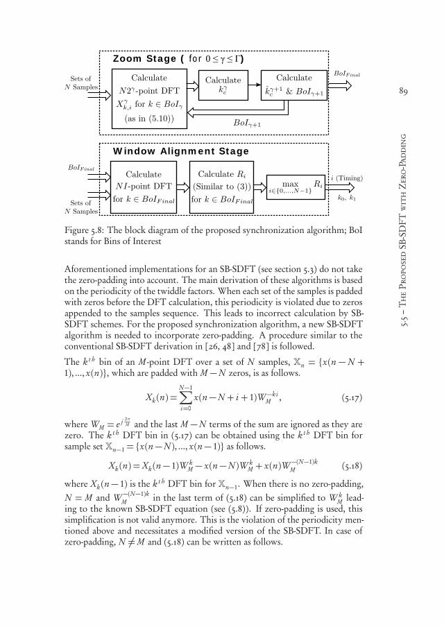
550999-L-bw-Siavash550999-L-bw-Siavash550999-L-bw-Siavash550999-L-bw-SiavashProcessed on: 23-11-2020Processed on: 23-11-2020Processed on: 23-11-2020Processed on: 23-11-2020 PDF page: 111PDF page: 111PDF page: 111PDF page: 111
89
5.5–TheProposedSB-SDFTwithZero-Padding
Zoom Stage ( for 0 ≤ γ ≤ Γ)
Window Alignment Stage
Figure 5.8: The block diagram of the proposed synchronization algorithm; BoIstands for Bins of Interest
Aforementioned implementations for an SB-SDFT (see section 5.3) do not takethe zero-padding into account. The main derivation of these algorithms is basedon the periodicity of the twiddle factors. When each set of the samples is paddedwith zeros before the DFT calculation, this periodicity is violated due to zerosappended to the samples sequence. This leads to incorrect calculation by SB-SDFT schemes. For the proposed synchronization algorithm, a new SB-SDFTalgorithm is needed to incorporate zero-padding. A procedure similar to theconventional SB-SDFT derivation in [26, 48] and [78] is followed.
The k t h bin of an M -point DFT over a set of N samples, Xn = x(n −N +1), ..., x(n), which are padded with M −N zeros, is as follows.
Xk (n) =N−1∑
i=0
x(n−N + i + 1)W −kiM , (5.17)
where WM = e j 2πM and the last M −N terms of the sum are ignored as they are
zero. The k t h DFT bin in (5.17) can be obtained using the k t h DFT bin forsample set Xn−1 = x(n−N ), ..., x(n− 1) as follows.
Xk (n) =Xk (n− 1)W kM − x(n−N )W k
M + x(n)W −(N−1)kM (5.18)
where Xk (n− 1) is the k t h DFT bin for Xn−1. When there is no zero-padding,N = M and W −(N−1)k
M in the last term of (5.18) can be simplified to W kM lead-
ing to the known SB-SDFT equation (see (5.8)). If zero-padding is used, thissimplification is not valid anymore. This is the violation of the periodicity men-tioned above and necessitates a modified version of the SB-SDFT. In case ofzero-padding, N =M and (5.18) can be written as follows.

550999-L-bw-Siavash550999-L-bw-Siavash550999-L-bw-Siavash550999-L-bw-SiavashProcessed on: 23-11-2020Processed on: 23-11-2020Processed on: 23-11-2020Processed on: 23-11-2020 PDF page: 112PDF page: 112PDF page: 112PDF page: 112
90
Chapter5–LowComplexityImplementationoftheFSKDemodulator
z-N
WM-kN WM
k
-z-1
x[n] Xk(n)
Figure 5.9: The modified SB-SDFT filter
Xk (n) =W kM (Xk (n− 1)− x(n−N )+ x(n)W −N k
M ) (5.19)
Equation (5.19) can be seen as a filter taking samples of x and generating the k t h
DFT bin while sliding the window by one sample. The transfer function of thefilter is:
H (z) =W −kN
M − z−N
W −kM − z−1
(5.20)
The block diagram of such a filter is also depicted in Figure 5.9. The SB-SDFTwith zero-padding has an extra multiplication in the first loop compared to theSB-SDFT in Figure 5.4. Similar to the conventional SB-SDFT in [48], it has apole on the unity circle. The stability of this modified version of SB-SDFT canbe guaranteed using a damping factor r (similar to the idea proposed in [48]).Another method is to extend this derivation to achieve a modified version of themodulated-SDFT introduced in [26]. The former compromises precision whilethe latter increases complexity almost twice. Using a damping factor causes anerror in the calculated DFT values. In our proposed method the exact value ofthe DFT is not the target but the relative value of different bins is important. Asa result, to avoid the complexity of the modulated-SDFT, the modified SB-SDFTmethod is stabilized by adding a damping factor. To change the pole from W k
Mto rW k
M , the z in (5.20) is replaced with z/r . This leads to the following transferfunction.
H (z) =W −kN
M − r N z−N
W −kM − r z−1
(5.21)
The block diagram of the stable filter is shown in Figure 5.10. For each loop, onemultiplication between a complex number and a real number is added which iscomposed of two real multiplications. The extra multiplications in the secondloop can be integrated into the twiddle factor. To do so, the nominator and thedenominator of the transfer function are multiplied with r−1 to achieve:
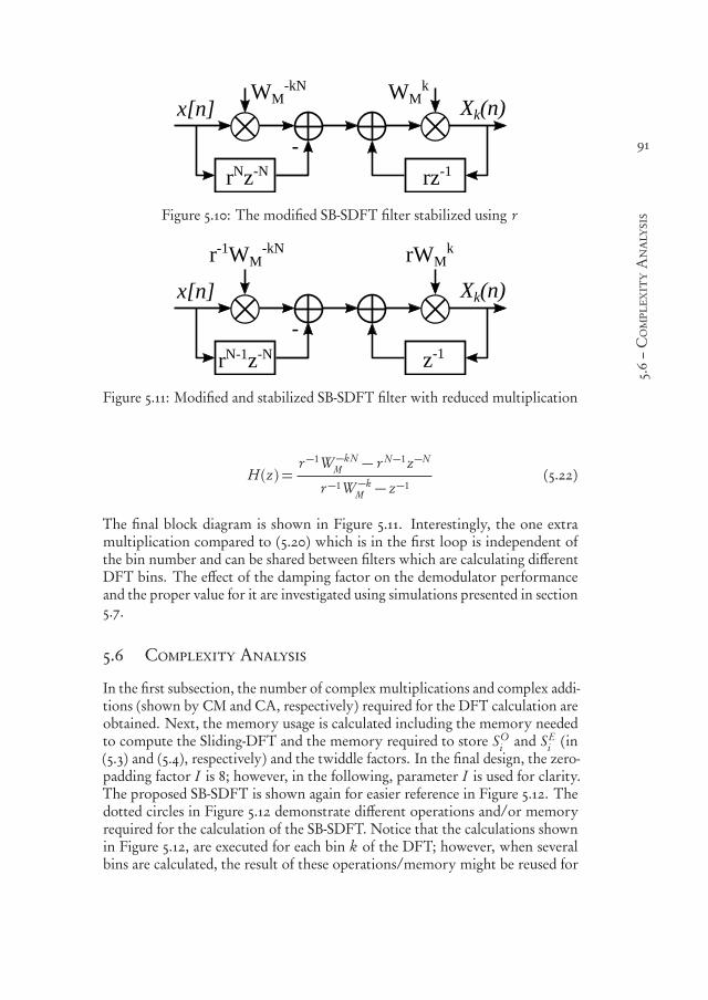
550999-L-bw-Siavash550999-L-bw-Siavash550999-L-bw-Siavash550999-L-bw-SiavashProcessed on: 23-11-2020Processed on: 23-11-2020Processed on: 23-11-2020Processed on: 23-11-2020 PDF page: 113PDF page: 113PDF page: 113PDF page: 113
91
5.6–ComplexityAnalysis
rNz-N
WM-kN WM
k
-rz-1
x[n] Xk(n)
Figure 5.10: The modified SB-SDFT filter stabilized using r
rN-1z-N
r-1WM-kN rWM
k
-z-1
x[n] Xk(n)
Figure 5.11: Modified and stabilized SB-SDFT filter with reduced multiplication
H (z) =r−1W −kN
M − r N−1z−N
r−1W −kM − z−1
(5.22)
The final block diagram is shown in Figure 5.11. Interestingly, the one extramultiplication compared to (5.20) which is in the first loop is independent ofthe bin number and can be shared between filters which are calculating differentDFT bins. The effect of the damping factor on the demodulator performanceand the proper value for it are investigated using simulations presented in section5.7.
5.6 Complexity Analysis
In the first subsection, the number of complex multiplications and complex addi-tions (shown by CM and CA, respectively) required for the DFT calculation areobtained. Next, the memory usage is calculated including the memory neededto compute the Sliding-DFT and the memory required to store SO
i and SEi (in
(5.3) and (5.4), respectively) and the twiddle factors. In the final design, the zero-padding factor I is 8; however, in the following, parameter I is used for clarity.The proposed SB-SDFT is shown again for easier reference in Figure 5.12. Thedotted circles in Figure 5.12 demonstrate different operations and/or memoryrequired for the calculation of the SB-SDFT. Notice that the calculations shownin Figure 5.12, are executed for each bin k of the DFT; however, when severalbins are calculated, the result of these operations/memory might be reused for

550999-L-bw-Siavash550999-L-bw-Siavash550999-L-bw-Siavash550999-L-bw-SiavashProcessed on: 23-11-2020Processed on: 23-11-2020Processed on: 23-11-2020Processed on: 23-11-2020 PDF page: 114PDF page: 114PDF page: 114PDF page: 114
92
Chapter5–LowComplexityImplementationoftheFSKDemodulator
rN-1z-N
r-1WM-kN rWM
k
-z-1
x[n] Xk(n)
A
B
C
D
E
FFigure 5.12: Modified and stabilized SB-SDFT filter with reduced multiplication
multiple bins i.e. that part of the block can be shared between a few bins. Thisis further explained in the following analysis wherever applicable.
5.6.1 Complex Operations
The complexity of the proposed method is separately calculated for the zoomand the window alignment stage while explaining the operations shown by thedotted circles of Figure 5.12. Each time that a new value for the DFT bin iscalculated is called an iteration. Each iteration updates the DFT value basedon the input sample and the last N − 1 samples of the input sequence (in totalN samples). In the following, multiplication and addition refer to complexoperations unless stated otherwise.
Zoom Stage:
A: The twiddle factor in A for the last step γ = Γ is r−1W −kNN I for bin k which is
written as r−1W −kI . Since WI = exp( j 2π/I ) is always a point on the unit circle
within the complex plane, its powers have only I different values regardless of thenumber of calculated bins. Since r−1W −(k+I/2)
I = −r−1W −kI , only half of the
twiddle factor multiplications, 0.5I , need to be calculated and the rest are simplysign conversions (multiplications with +/- j are still considered as a completecomplex multiplication). The last step of the zoom stage has the largest zero-padding factor and consequently, the largest number of different twiddle factors.So the number of multiplications within operationA is the largest in the last step.To simplify the complexity expressions we consider 0.5I multiplications for theother steps of the zoom stage as well. So A leads to (0.5I )(Γ +1) multiplicationsper iteration for all bins and all steps together.
B: The operation in B is a real-by-complex multiplication and we approximateit by 0.5 complex multiplication. It can be shared between all bins at each step.For all steps together, it leads to 0.5(Γ +1)multiplications for each iteration andall bins together.

550999-L-bw-Siavash550999-L-bw-Siavash550999-L-bw-Siavash550999-L-bw-SiavashProcessed on: 23-11-2020Processed on: 23-11-2020Processed on: 23-11-2020Processed on: 23-11-2020 PDF page: 115PDF page: 115PDF page: 115PDF page: 115
93
5.6.1–ComplexOperations
C: Based on the above discussion, the output of A may have at most I differentvalues in each step for all bins and B can be shared with all bins. As a result, C,leads to I additions (at most) per iteration in each step for all bins together. SoC leads to I (Γ + 1) additions per iteration for all bins and all steps together.
D/E: These parts together include one multiplication and one addition per binand per iteration. In the zoom stage, at the first step, N bins are calculated and forthe other Γ steps I bins are calculated (N+I Γ in total). Thus, for the zoom stage,per iteration and for all bins together D and E lead to N + I Γ multiplicationsand additions, respectively.
Iterations: remember that for each step of the zoom stage the window shifts 2Nsamples (i.e. 2N iterations). Starting from the initial state of zero, N iterationsare required to generate the DFT value for the first window of N samples. Then,each iteration gives the SB-SDFT for the next window. As a result, there are 3Niterations for each bin at each step of the zoom stage. Now, considering the abovediscussion and the number of iterations, the total number of multiplications andadditions for the zoom stage (C MZoom and C AZoom , respectively) are obtainedas follows.
C MZoom = 3N (0.5(I + 1)(Γ + 1)+ (N + I Γ )) (5.23)
C AZoom = 3N (I (Γ + 1)+ (N + I Γ )) (5.24)
Window Alignment Stage:
A: In the window alignment stage, the zero-padding factor is I . Following thesame reasoning as the zoom stage, A needs 0.5I multiplications per iteration forall bins together.
B: In total, this part needs two real multiplications or 0.5 complex multiplicationper iteration for all bins together.
C: Similar to what was mentioned for the zoom stage, C leads to I complexadditions per iteration for all bins together.
D/E: In the window alignment stage, |BoIF i nal | bins are calculated. Thus, periteration and for all bins together D and E lead to |BoIF i nal | multiplications andadditions, respectively.
Iterations: The window alignment stage needs N (L− 1) iterations where L isthe length of the preamble 2. Following the same reasoning as for the zoomstage, N extra iterations are required when starting from the initial state ofzero so the alignment stage needs N L iterations for each bin. The number ofmultiplications and additions for the window alignment stage (C MAl i g n andC AAl i g n , respectively) are:
2N delays for each symbol, from symbol 1 to symbol L− 1 of the preamble.

550999-L-bw-Siavash550999-L-bw-Siavash550999-L-bw-Siavash550999-L-bw-SiavashProcessed on: 23-11-2020Processed on: 23-11-2020Processed on: 23-11-2020Processed on: 23-11-2020 PDF page: 116PDF page: 116PDF page: 116PDF page: 116
94
Chapter5–LowComplexityImplementationoftheFSKDemodulator
C MAl i g n =N L(0.5(I + 1)+ |BoIF i nal |) (5.25)
C AAl i g n =N L(I + |BoIF i nal |) (5.26)
5.6.2 Memory
Since the zoom stage and the window alignment stage are not executed in parallel,the registers (memory elements) used in one can be used in the other as well.Here, we only focus on the window alignment stage as it needs more memoryand therefore, dictates the total required memory for calculating the SDFT. Forthe Sliding DFT each filter needs a memory of size N for samples and a delayof one for the previous DFT value (See B and F in Figure 5.11). The memorywithin B ( z−N with length N ) can be shared between all bins and the second isunique for each bin. Additionally, the delay block in Figure 5.6 requires storing2N (Γ + 1) samples. All these values have two parts (real and imaginary), so therequired memory for calculating SDFT (MC al c ) is as follows.
MC al c = 2(N + |BoIF i nal |+ 2N (Γ + 1)) (5.27)
where |BoIF i nal | is the cardinality of the set of BoI used in the window alignmentstage. The proposed synchronization algorithm needs to store the results of theaccumulation of the DFT magnitudes for |BoIF i nal | bins and N delay values.This memory is denoted by MAcc and is derived as follows.
MAcc = 2|BoIF i nal |N (5.28)
The factor two comes from the two sets of magnitudes that must be accumulatedfor odd and even symbols.
For an N I -point DFT, WN I = exp( j 2πN I ) which means that W −k
N I takes N I dif-ferent values. Since W −(k+N I/2)
N I = −W −kN I , only half of these values should be
stored from which two values are equal to 1 and j for k = 0 and k = N I/4,respectively. As a result, N I/2− 2 complex twiddle factors should be stored sothe required memory is N I − 4.
5.6.3 Comparison
As mentioned in section 5.3, the SFFT method in [30] provides an efficientimplementation of the Hara synchronization algorithm. The complexity of theSFFT for each iteration can be found in [30]. Due to zero-padding, in a fewfirst stages of the SFFT some operations have zero inputs and are not executedwhich leads to a pruned structure with reduced complexity. The number ofiterations for the SFFT in the Hara synchronization algorithm can be derivedbased on a reasoning similar to what was used above for the window alignmentstage. Taking these into account, the complexity of the Hara synchronization

550999-L-bw-Siavash550999-L-bw-Siavash550999-L-bw-Siavash550999-L-bw-SiavashProcessed on: 23-11-2020Processed on: 23-11-2020Processed on: 23-11-2020Processed on: 23-11-2020 PDF page: 117PDF page: 117PDF page: 117PDF page: 117
95
5.7–SimulationResultsandDiscussion
can be calculated. The detailed calculations are included in Appendix B and onlythe final results are presented here for comparison.
The number of operations and memory required for the Hara synchronizationand the proposed synchronization algorithms are presented in Table 5.2. Forthe total number of operations only the term with the largest power of N isincluded in the table. Although the number of CM/CA increases with N 2 forboth methods, in practical cases, the factor of N 2 in the Hara method is muchlarger than that of the proposed method. Considering L = 16 and I = 8, thefactor of N 2 in the number of complex multiplications required for the Harasynchronization (implemented using SFFT) is more than 40 times the factor ofN 2 in the complexity of the proposed synchronization algorithm. Furthermore,the total memory of the Hara method (with SFFT) increases with N 2 whilethe total memory of the proposed method increases with N . These differencesbetween the complexity stem from the fact that in the proposed synchroniza-tion algorithm, in contrast with the Hara synchronization, the number of thecalculated DFT bins for the window alignment does not change with N and isconstant (BoIF i nal ). The numerical results and comparison of complexity fordifferent values of N are presented in the next section.
5.7 Simulation Results and Discussion
5.7.1 Design Parameters
According to our discussions in the previous sections, two parameters need yet tobe determined. Those are the number of bins in the BoIF i nal and the dampingfactor r for the SB-SDFT. The most important performance metric for oursystem is the overall BER of the demodulator. Therefore, BER values obtainedby simulations are utilized to determine the appropriate design parameters. Asstated in 5.4, in all simulations of this section I = 8 and L = 16 similar toChapter 3. Figure 5.13 shows how the BER of the demodulator changes relativeto |BoIF i nal | for different values of Eb/N0. The damping factor is consideredto be r = 1 in these simulations. As can be seen in Figure 5.13, the bit errorrate value hardly changes when the number of bins in the BoIF i nal is increasedto more than 14. For a safety margin the number of bins in the BoIF i nal isconsidered to be 16.
The value of the damping factor determines the error at the output of the SB-SDFT filter. As mentioned earlier, the damping factor introduces errors to thecalculated values for the DFT which may degrade the performance of the demod-ulator. This can be solved by choosing r very close to one. Additionally, thenumber of samples which pass through the SB-SDFT filter plays an importantrole in the value of r . Due to the recursive behavior of the filter, the error accu-mulation increases when an SB-SDFT is applied to a long sequence of samples.Thus, for a constant preamble length, the appropriate value for r also dependson the number of samples per symbol. As explained in Chapter 3, N is propor-

550999-L-bw-Siavash550999-L-bw-Siavash550999-L-bw-Siavash550999-L-bw-SiavashProcessed on: 23-11-2020Processed on: 23-11-2020Processed on: 23-11-2020Processed on: 23-11-2020 PDF page: 118PDF page: 118PDF page: 118PDF page: 118
96
Chapter5–LowComplexityImplementationoftheFSKDemodulator
Table5.2:C
omplexity
comparison.
Listhe
lengthofthe
preamble,I
isthezero-padding
factor,Nisthe
number
ofsamplesper
symboland
BoIF
inal isthenum
berofbinsused
inthe
window
alignmentstage
oftheproposed
synchronization.Forsim
ulationresultspresented
insection
5.7,L=
16,I=
8,Γ=
3and
BoIF
inal =16.
Hara
synchronization(w
ithSFFT
)Proposed
synchronization(w
ithSB-SD
FT)
Zoom
Align
DFT
Calculation
CM
I(N−
1)NL
3N(0.5(I+
1)(Γ+
1)+N+
IΓ)N
L(0.5(I+1)+|B
oIFinal |)
CA
2I(N−
1)NL
3N(I(Γ+
1)+N+
IΓ)N
L(I+|B
oIFinal |)
TotalOperations
CM
ILN2+
...ILN
2+...
ILN2+
...3N
2+...
3N2+
...3N
2+...
CA
2ILN2+
...2ILN
2+...
2ILN2+
...3N
2+...
3N2+
...3N
2+...
Mem
oryCalc
2NIlog
2 N−(4I−
2)(N−
1)(4Γ+
6)N+
2|BoIF
inal |Acc
2IN2
2|BoIF
inal |NTw
iddleN
I−4
NI−
4
TotalMem
ory2IN(N+
log2 N)+
...2IN(N+
log2 N)+
...2IN(N+
log2 N)+
...(I+
4Γ+
2|BoIF
inal |+6)N+
...(I+
4Γ+
2|BoIF
inal |+6)N+
...(I+
4Γ+
2|BoIF
inal |+6)N+
...
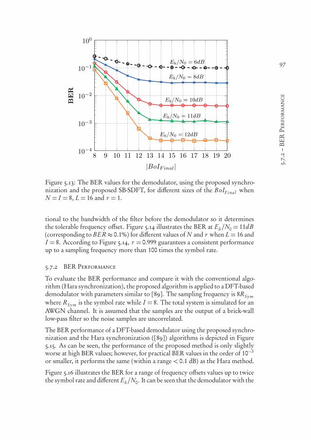
550999-L-bw-Siavash550999-L-bw-Siavash550999-L-bw-Siavash550999-L-bw-SiavashProcessed on: 23-11-2020Processed on: 23-11-2020Processed on: 23-11-2020Processed on: 23-11-2020 PDF page: 119PDF page: 119PDF page: 119PDF page: 119
97
5.7.2–BERPerformance
8 9 10 11 12 13 14 15 16 17 18 19 2010−4
10−3
10−2
10−1
100
Eb/N0 = 6dB
Eb/N0 = 8dB
Eb/N0 = 10dB
Eb/N0 = 11dB
Eb/N0 = 12dB
|BoIFinal|
BER
Figure 5.13: The BER values for the demodulator, using the proposed synchro-nization and the proposed SB-SDFT, for different sizes of the BoIF i nal whenN = I = 8, L= 16 and r = 1.
tional to the bandwidth of the filter before the demodulator so it determinesthe tolerable frequency offset. Figure 5.14 illustrates the BER at Eb/N0 = 11dB(corresponding to BER≈ 0.1%) for different values of N and r when L= 16 andI = 8. According to Figure 5.14, r = 0.999 guarantees a consistent performanceup to a sampling frequency more than 100 times the symbol rate.
5.7.2 BER Performance
To evaluate the BER performance and compare it with the conventional algo-rithm (Hara synchronization), the proposed algorithm is applied to a DFT-baseddemodulator with parameters similar to [89]. The sampling frequency is 8RSy mwhere RSy m is the symbol rate while I = 8. The total system is simulated for anAWGN channel. It is assumed that the samples are the output of a brick-walllow-pass filter so the noise samples are uncorrelated.
The BER performance of a DFT-based demodulator using the proposed synchro-nization and the Hara synchronization ( [89]) algorithms is depicted in Figure5.15. As can be seen, the performance of the proposed method is only slightlyworse at high BER values; however, for practical BER values in the order of 10−3
or smaller, it performs the same (within a range < 0.1 dB) as the Hara method.
Figure 5.16 illustrates the BER for a range of frequency offsets values up to twicethe symbol rate and different Eb/N0. It can be seen that the demodulator with the
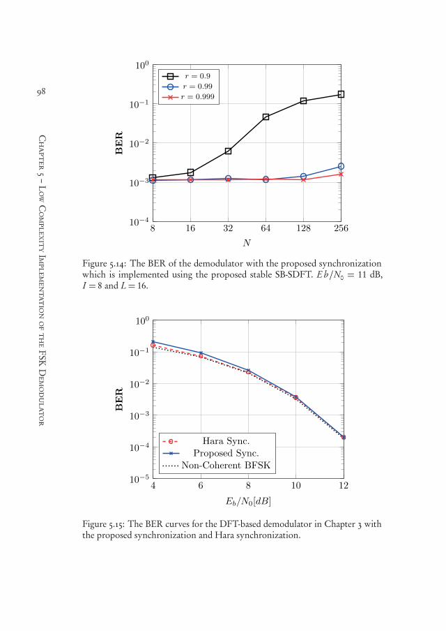
550999-L-bw-Siavash550999-L-bw-Siavash550999-L-bw-Siavash550999-L-bw-SiavashProcessed on: 23-11-2020Processed on: 23-11-2020Processed on: 23-11-2020Processed on: 23-11-2020 PDF page: 120PDF page: 120PDF page: 120PDF page: 120
98
Chapter5–LowComplexityImplementationoftheFSKDemodulator
8 16 32 64 128 25610−4
10−3
10−2
10−1
100
N
BER
r = 0.9
r = 0.99
r = 0.999
Figure 5.14: The BER of the demodulator with the proposed synchronizationwhich is implemented using the proposed stable SB-SDFT. E b/N0 = 11 dB,I = 8 and L= 16.
4 6 8 10 1210−5
10−4
10−3
10−2
10−1
100
Eb/N0[dB]
BER
Hara Sync.Proposed Sync.
Non-Coherent BFSK
Figure 5.15: The BER curves for the DFT-based demodulator in Chapter 3 withthe proposed synchronization and Hara synchronization.

550999-L-bw-Siavash550999-L-bw-Siavash550999-L-bw-Siavash550999-L-bw-SiavashProcessed on: 23-11-2020Processed on: 23-11-2020Processed on: 23-11-2020Processed on: 23-11-2020 PDF page: 121PDF page: 121PDF page: 121PDF page: 121
99
5.7.3–Complexity
−2 −1.5 −1 −0.5 0 0.5 1 1.5 210−4
10−3
10−2
10−1
100
Eb/N0 = 6dB
Eb/N0 = 8dB
Eb/N0 = 10dB
Eb/N0 = 12dB
foffsetT
BER
Figure 5.16: The BER of the demodulator with the proposed synchronization al-gorithm for different frequency offsets normalized to the symbol rate ( fo f f s e t T ).
proposed synchronization algorithm can tolerate frequency offset as expected.
Figure 5.17 shows the BER performance of the proposed method for differentvalues of N and Eb/N0. For these simulations I = 8, L = 16 and r = 0.999.It is seen that the increase of N does not affect the BER performance of thedemodulator using the proposed synchronization algorithm and the proposedSB-SDFT. Notice that increasing N means that the bandwidth of the filter priorto the demodulator increases (see discussion in Chapter 3). This means that thenoise bandwidth increases. As can be seen in the results, this increased noisebandwidth does not degrade the BER performance. This can be justified bylooking at the DFT as a bank of narrowband filters as discussed in Chapter 3.
Finally, Figure 5.18 illustrates the performance of the demodulator with theproposed synchronization in Rayleigh and Rician fading (K = 4) channels. Itcan be seen that a demodulator using the proposed synchronization performsthe same as a demodulator with Hara synchronization algorithm.
5.7.3 Complexity
Figure 5.19 shows the number of complex operations and memory requiredfor both methods and different values of N while I = 8, |BoIF i nal | = 16 andL = 16 (both axes are on logarithmic scale). Furthermore, Figure 5.20 showsthe improvement achieved using the proposed algorithm and SB-SDFT. Theimprovement is defined as the percentage of the reduced operations relative to
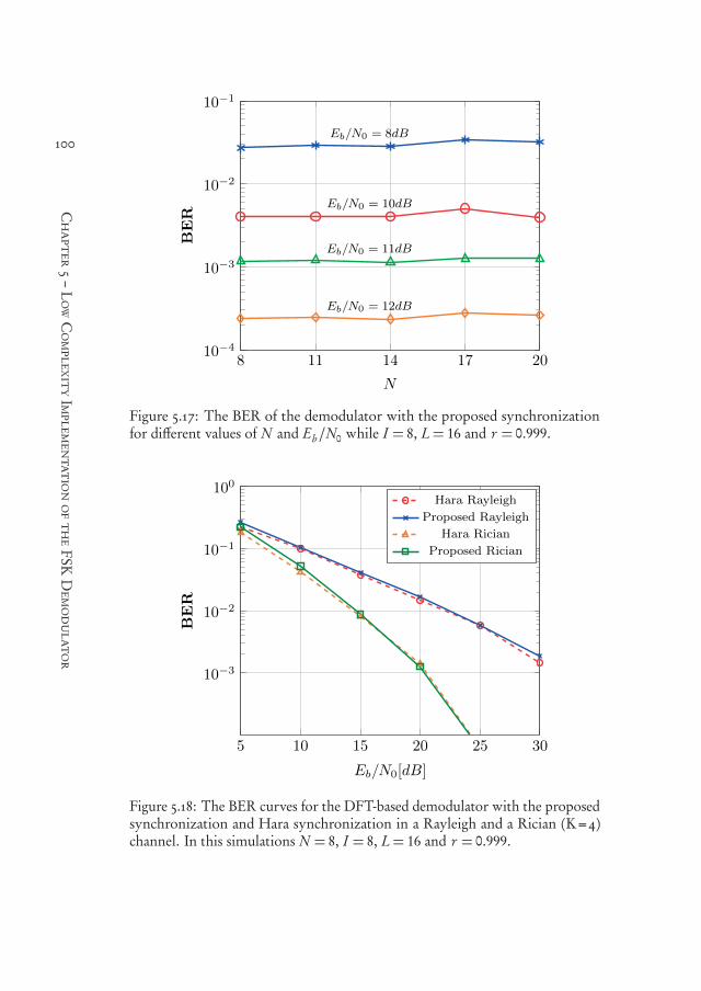
550999-L-bw-Siavash550999-L-bw-Siavash550999-L-bw-Siavash550999-L-bw-SiavashProcessed on: 23-11-2020Processed on: 23-11-2020Processed on: 23-11-2020Processed on: 23-11-2020 PDF page: 122PDF page: 122PDF page: 122PDF page: 122
100
Chapter5–LowComplexityImplementationoftheFSKDemodulator
8 11 14 17 2010−4
10−3
10−2
10−1
Eb/N0 = 8dB
Eb/N0 = 10dB
Eb/N0 = 11dB
Eb/N0 = 12dB
N
BER
Figure 5.17: The BER of the demodulator with the proposed synchronizationfor different values of N and Eb/N0 while I = 8, L= 16 and r = 0.999.
5 10 15 20 25 30
10−3
10−2
10−1
100
Eb/N0[dB]
BER
Hara Rayleigh
Proposed Rayleigh
Hara Rician
Proposed Rician
Figure 5.18: The BER curves for the DFT-based demodulator with the proposedsynchronization and Hara synchronization in a Rayleigh and a Rician (K=4)channel. In this simulations N = 8, I = 8, L= 16 and r = 0.999.
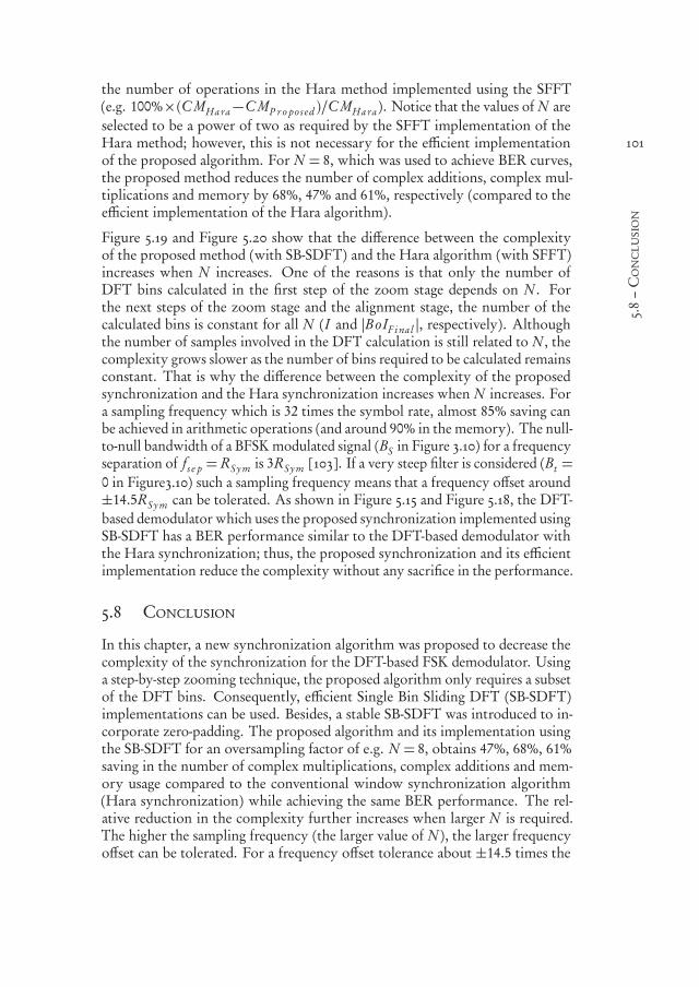
550999-L-bw-Siavash550999-L-bw-Siavash550999-L-bw-Siavash550999-L-bw-SiavashProcessed on: 23-11-2020Processed on: 23-11-2020Processed on: 23-11-2020Processed on: 23-11-2020 PDF page: 123PDF page: 123PDF page: 123PDF page: 123
101
5.8–Conclusion
the number of operations in the Hara method implemented using the SFFT(e.g. 100%×(C MH a ra−C MP r o pos ed )/C MH a ra ). Notice that the values of N areselected to be a power of two as required by the SFFT implementation of theHara method; however, this is not necessary for the efficient implementationof the proposed algorithm. For N = 8, which was used to achieve BER curves,the proposed method reduces the number of complex additions, complex mul-tiplications and memory by 68%, 47% and 61%, respectively (compared to theefficient implementation of the Hara algorithm).
Figure 5.19 and Figure 5.20 show that the difference between the complexityof the proposed method (with SB-SDFT) and the Hara algorithm (with SFFT)increases when N increases. One of the reasons is that only the number ofDFT bins calculated in the first step of the zoom stage depends on N . Forthe next steps of the zoom stage and the alignment stage, the number of thecalculated bins is constant for all N ( I and |BoIF i nal |, respectively). Althoughthe number of samples involved in the DFT calculation is still related to N , thecomplexity grows slower as the number of bins required to be calculated remainsconstant. That is why the difference between the complexity of the proposedsynchronization and the Hara synchronization increases when N increases. Fora sampling frequency which is 32 times the symbol rate, almost 85% saving canbe achieved in arithmetic operations (and around 90% in the memory). The null-to-null bandwidth of a BFSKmodulated signal (BS in Figure 3.10) for a frequencyseparation of fs e p = RSy m is 3RSy m [103]. If a very steep filter is considered (Bt =0 in Figure3.10) such a sampling frequency means that a frequency offset around±14.5RSy m can be tolerated. As shown in Figure 5.15 and Figure 5.18, the DFT-based demodulator which uses the proposed synchronization implemented usingSB-SDFT has a BER performance similar to the DFT-based demodulator withthe Hara synchronization; thus, the proposed synchronization and its efficientimplementation reduce the complexity without any sacrifice in the performance.
5.8 Conclusion
In this chapter, a new synchronization algorithm was proposed to decrease thecomplexity of the synchronization for the DFT-based FSK demodulator. Usinga step-by-step zooming technique, the proposed algorithm only requires a subsetof the DFT bins. Consequently, efficient Single Bin Sliding DFT (SB-SDFT)implementations can be used. Besides, a stable SB-SDFT was introduced to in-corporate zero-padding. The proposed algorithm and its implementation usingthe SB-SDFT for an oversampling factor of e.g. N = 8, obtains 47%, 68%, 61%saving in the number of complex multiplications, complex additions and mem-ory usage compared to the conventional window synchronization algorithm(Hara synchronization) while achieving the same BER performance. The rel-ative reduction in the complexity further increases when larger N is required.The higher the sampling frequency (the larger value of N ), the larger frequencyoffset can be tolerated. For a frequency offset tolerance about ±14.5 times the
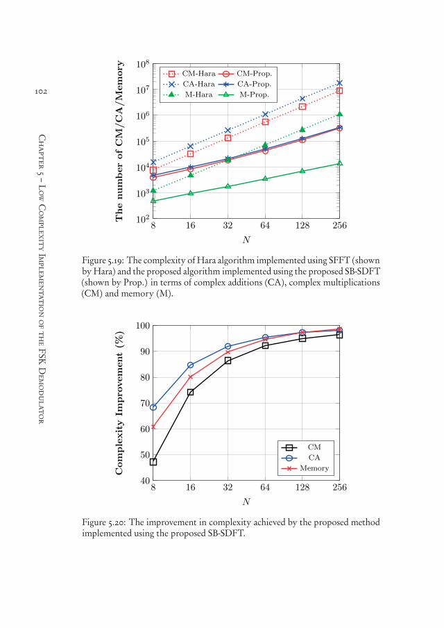
550999-L-bw-Siavash550999-L-bw-Siavash550999-L-bw-Siavash550999-L-bw-SiavashProcessed on: 23-11-2020Processed on: 23-11-2020Processed on: 23-11-2020Processed on: 23-11-2020 PDF page: 124PDF page: 124PDF page: 124PDF page: 124
102
Chapter5–LowComplexityImplementationoftheFSKDemodulator
8 16 32 64 128 256102
103
104
105
106
107
108
N
ThenumberofCM
/CA/M
emory
CM-Hara CM-Prop.
CA-Hara CA-Prop.
M-Hara M-Prop.
Figure 5.19: The complexity of Hara algorithm implemented using SFFT (shownbyHara) and the proposed algorithm implemented using the proposed SB-SDFT(shown by Prop.) in terms of complex additions (CA), complex multiplications(CM) and memory (M).
8 16 32 64 128 25640
50
60
70
80
90
100
N
ComplexityIm
pro
vement(%
)
CM
CA
Memory
Figure 5.20: The improvement in complexity achieved by the proposed methodimplemented using the proposed SB-SDFT.

550999-L-bw-Siavash550999-L-bw-Siavash550999-L-bw-Siavash550999-L-bw-SiavashProcessed on: 23-11-2020Processed on: 23-11-2020Processed on: 23-11-2020Processed on: 23-11-2020 PDF page: 125PDF page: 125PDF page: 125PDF page: 125
103
5.8–Conclusion
symbol rate which requires an oversampling factor N = 32, the number of com-plex operations is reduced by more than 85% (and memory by 90%) comparedto the conventional method (Hara synchronization implemented using SFFT).

550999-L-bw-Siavash550999-L-bw-Siavash550999-L-bw-Siavash550999-L-bw-SiavashProcessed on: 23-11-2020Processed on: 23-11-2020Processed on: 23-11-2020Processed on: 23-11-2020 PDF page: 126PDF page: 126PDF page: 126PDF page: 126
104

550999-L-bw-Siavash550999-L-bw-Siavash550999-L-bw-Siavash550999-L-bw-SiavashProcessed on: 23-11-2020Processed on: 23-11-2020Processed on: 23-11-2020Processed on: 23-11-2020 PDF page: 127PDF page: 127PDF page: 127PDF page: 127
1056Hybrid Modulation
and Time Diversity
Abstract – Carrier frequency offset (CFO) and time-varying fading chan-nels are two problems that ultra-narrowband solutions for the emerging LowPower Wide Area Networks (LPWAN) need to tackle. To overcome CFO,offset tolerant demodulators have been proposed for both PSK and FSK mod-ulations. To combat channel distortion, time or frequency diversity togetherwith coding techniques can be utilized. To afford the redundancy required forthese solutions, a lower effective bit-rate has to be accepted or a higher bit-rateis required. Higher order PSK and FSK considerably compromise energy andbandwidth, respectively. As a third solution, hybrid modulation has been pro-posed which can increase the bit-rate in a more power and bandwidth efficientway than PSK and FSK, respectively. In this work, an offset tolerant demod-ulator is proposed for hybrid modulations combining Double DifferentialM-ary PSK (DDMPSK) and Differential L-ary FSK (DLFSK). The proposeddemodulator is evaluated for different combinations of M and L in a time-varying channel using a time diversity technique. Through different scenariosthe hybrid demodulator is compared to DDMPSK. The results demonstratethat at BER=0.1%, the hybrid modulation can improve BER performancecompared to higher order DDMPSK in all scenarios.
6.1 Introduction
In the previous chapters, offset tolerant demodulators were investigated to over-come Carrier Frequency Offset (CFO) in UNB communication systems. Inaddition to CFO, UNB systems are vulnerable to temporal fading due to theirlong symbol time. As shown in [71], for a low data rate system, a time-varyingchannel can even cause an error floor. As a consequence of time-varying behav-
This chapter is based on [S:1] and [S:5].
550999-L-bw-Siavash550999-L-bw-Siavash550999-L-bw-Siavash550999-L-bw-SiavashProcessed on: 23-11-2020Processed on: 23-11-2020Processed on: 23-11-2020Processed on: 23-11-2020 PDF page: 128PDF page: 128PDF page: 128PDF page: 128
106
Chapter6–HybridModulationandTimeDiversity
ior, channel estimation at the beginning of a packet is not reliable. Furthermore,using multiple pilot sequences for channel estimation imposes prohibitive over-head due to short packets used in these systems (as short as 200 symbols [38, 55]).
In such circumstances, diversity techniques can be utilized to improve perfor-mance [71]. Space diversity requires multiple antennas and RF chains whichmakes it improper for a low power and area constrained receiver. Frequencydiversity using techniques such as frequency hopping is another option. In ahighly time-variant channel, time diversity can be achieved using channel codingand interleaving. In either of these two techniques redundant information mustbe transmitted.
As discussed in the previous chapters, offset tolerant demodulators have beenproposed for both FSK and PSKmodulations and they can be employed in UNBcommunication systems which are susceptible to CFO. However, transmittingredundant information increases either the time required to transmit a packet ofinformation bits or the bit-rate. Longer transmission time, increases on-time ofthe RF front-end which plays a significant role in the overall power consumption.Therefore, a higher raw bit-rate is preferred. One solution is using higher orderPSK. The downside of this solution is loss in the BER performance. As analternative a higher order FSK can be employed which compromises bandwidthfor a better BER performance. Hybrid frequency/phase modulation is a thirdpossible solution which has been suggested in literature [17, 34, 35, 52, 57, 87].
In this chapter, an offset-tolerant modulator and demodulator for hybrid mod-ulation is proposed to tackle frequency offset and temporal fading at the sametime. The demodulator is designed for a combination of LFSK and MPSK. Toget insight into the performance of the hybrid modulation, the demodulatoris evaluated for various combinations of MPSK and LFSK while time-varyingRayleigh and Rician channel models are considered. Moreover, the bandwidthcompromise of the hybrid modulation compared to PSK modulation is takeninto account through investigating an equal bandwidth scenario.
The rest of this chapter is organized as follows. The next section reviews existingwork on the hybrid modulation technique. Section 6.3 elaborates on the designof the hybrid demodulator in the general cases of MPSK and LFSK and its tolera-ble frequency offset. Amathematical formulation and error floor expressions arepresented in section 6.4 to show how the proposed demodulator performs in atime-varying channel and why using FSK is better than solely using higher orderPSK. The system including time diversity is designed and explicated in section6.5. Simulation results and discussions for an AWGN channel and a time-varyingchannel with different scenarios are included in sections 6.6 and 6.7, respectively.Finally, section 6.8 concludes this chapter.

550999-L-bw-Siavash550999-L-bw-Siavash550999-L-bw-Siavash550999-L-bw-SiavashProcessed on: 23-11-2020Processed on: 23-11-2020Processed on: 23-11-2020Processed on: 23-11-2020 PDF page: 129PDF page: 129PDF page: 129PDF page: 129
107
6.2–RelatedWork
6.2 Related Work
As mentioned in Chapter 1 and Chapter 2, the hybrid frequency/phase modu-lation has been investigated as an alternative option to change the power andbandwidth efficiency trade-off of higher order PSK and FSK. A combination ofLFSK and MPSK can benefit from the energy efficiency of higher order FSKwhile it alleviates the LFSK spectral deficiency with higher order PSK.
One of the early examples of frequency/phase modulation (FPSK) was proposedin [87]. This idea was later formulated in [59, 93] as an L-orthogonal signalingmethod where both frequency and phase are modulated. For FPSK signals tobe orthogonal for any order of phase modulation, the frequency separationshould be equal to the symbol rate [34, 93]. In [52], a signal is generated bycombining N different frequencies each of which is modulated using one of theM possible phases of MPSK and a coherent receiver for such modulation schemeis proposed. Using various combinations of frequency tones and phase mod-ulation, M N different modulated signals can be generated. For higher energyefficiency, a modification to the proposed modulation is introduced called expur-gated phase codes. It only uses combinations which have minimum correlation[52]. This modified version decreases bandwidth efficiency but improves theBER performance. Using only half of the code combinations (E4-FPSK) themodified version can achieve more than 4 dB improvement compared to 8PSKwhich provides the same modulation order. The bandwidth efficiency is thoughdecreased by 30%.
In [34], a non-coherent demodulator for a frequency/phase modulation schemeis proposed using non-coherent FSK and Differential PSK (DPSK). During eachsymbol, the frequency is modulated with one of the L possible tones of LFSKand phase is differentially modulated with MPSK. It is shown that using a combi-nation of FSK and DPSK requires lower Eb/N0 compared to higher order PSKwhen achieving the same BER performance. For instance, using a combinationof BFSK and QPSK instead of 8PSK, which provides the same modulation order,achieves almost 6 dB energy saving at BER=0.1% [34]. This improvement isachieved at the cost of 30% decrease in bandwidth efficiency. The performanceof FPSK in slow and flat fading channels is investigated in [35]. It shows that, ina flat and slow Rayleigh fading channel, FPSK is still better than higher orderPSK but the improvement achieved in the BER performance is less compared towhat is achieved in an AWGN channel.
Despite all the work in literature, no offset tolerant demodulator has been de-signed for the FPSK modulation scheme capable of tolerating CFO which ismuch larger than the symbol rate. Furthermore, the performance of FPSK in atime-varying channel has not been investigated. In this chapter, an offset tolerantdemodulator is designed for the frequency/phase modulation (FPSK) and its per-formance in a time-varying channel using a time diversity scheme is evaluated.The next section elaborates on the design of the modulator, demodulator and

550999-L-bw-Siavash550999-L-bw-Siavash550999-L-bw-Siavash550999-L-bw-SiavashProcessed on: 23-11-2020Processed on: 23-11-2020Processed on: 23-11-2020Processed on: 23-11-2020 PDF page: 130PDF page: 130PDF page: 130PDF page: 130
108
Chapter6–HybridModulationandTimeDiversity
Table 6.1: Parameters and notation
FSK order L
PSK order M
Symbol rate RS
Bit-rate Rb
Energy per symbol ES
Energy per bit Eb
Energy per information bit E I n fb
Sampling time Ts
Sampling frequency Fs
Symbol duration T
FSK frequency separation fs e p
n t h symbol modulated frequency ωn = 2π fn
n t h symbol modulated phase ϕn
Packet length LP
Frequency offset ωO = 2π fO
Samples per symbol N
the range of tolerable frequency offset.
6.3 Offset Tolerant Hybrid Demodulator
The proposed offset tolerant demodulator makes it possible to employ hybridmodulation in applications which are susceptible to large frequency offset (mul-tiple times the symbol rate). To explain offset tolerant demodulator design, firstthe hybrid modulator is explained. Then, an offset tolerant demodulator for thismodulation is achieved and the range of frequency offset that can be tolerated isanalyzed.
6.3.1 Modulator Design
For offset tolerant hybrid modulation, a combination of Differential LFSK(DLFSK) and Double Differential MPSK (DDMPSK) is utilized. These tech-niques and the reason for choosing differential and double differential encodingwill be clarified later when the demodulator is derived. The parameters andsymbols used in the signal model are summarized in Table 6.1.
A hybrid modulator modulates both phase and frequency based on the transmit-ted bits. The block diagram of the proposed modulator is shown in Figure 6.1a.The modulator receives two sets of bits; BF SK is the set of bits modulated over

550999-L-bw-Siavash550999-L-bw-Siavash550999-L-bw-Siavash550999-L-bw-SiavashProcessed on: 23-11-2020Processed on: 23-11-2020Processed on: 23-11-2020Processed on: 23-11-2020 PDF page: 131PDF page: 131PDF page: 131PDF page: 131
109
6.3.2–DemodulatorDesign
FSK and BP SK is the set of bits modulated using PSK. In the upper branch, asimple MPSK modulator and double differential encoder are used. First, the bitsare mapped to symbols to achieve αn = 2πm/M which is the modulated phasefor the n t h symbol and m = 0, ..., M − 1. Then, mapped symbols go throughtwo cascaded differential encoders to generate e jβn and e jϕn , respectively. e jϕn
is the phase of transmitted DDMPSK signal during the n t h symbol. In eachdifferential encoder the modulated MPSK signal is multiplied with its delayedversion (one symbol period delay). The relations between α, β and ϕ are asfollows.
αn =βn −βn−1
βn = ϕn −ϕn−1 (6.1)
In the lower branch, bits are mapped to integers (symbols), γn , which correspondto the frequency indexes of an LFSK modulation; γn ∈ 0, ..., L− 1. In the LFSKdifferential demodulator (explained later) the difference between two consecutivesymbol frequencies is detected; thus, the symbols should be coded into thedifference of consecutive symbol frequencies. For this purpose a differentialencoder is applied to the frequency index γn to generate the final transmittedfrequency index as follows.
λn = (γn +λn−1)mod (L) (6.2)
In (6.2), (x)mod (L) shows the remainder of x divided by L. When the index isdetermined, the frequency of LFSK during the n t h symbol period is obtained asfollows.
fn =− fs e p/2+(λn + 1− L/2) fs e p (6.3)
where fs e p is the FSK frequency separation. Using (6.1) and (6.3), the basebandequivalent of the transmitted signal during the n t h symbol, s(t ) , is as follows.
s(t ) =Æ
ES/T exp[ j (ωn t +ϕn +θn)], (n− 1)T ≤ t < nT (6.4)
where 2π fn is replaced by ωn for easier notation and θn is the initial phase atthe beginning of the n t h symbol including a constant phase offset. Similar toother frequency/phase modulation schemes, the frequency separation of LFSKis considered to be equal to the symbol rate to guarantee orthogonality [34].
6.3.2 Demodulator Design
To derive the proposed offset tolerant demodulator for the hybrid modulation,we start with the samples of the signal at the input of the demodulator. Here,we assume that the sampling frequency Fs =N RS , is an integer multiple of the

550999-L-bw-Siavash550999-L-bw-Siavash550999-L-bw-Siavash550999-L-bw-SiavashProcessed on: 23-11-2020Processed on: 23-11-2020Processed on: 23-11-2020Processed on: 23-11-2020 PDF page: 132PDF page: 132PDF page: 132PDF page: 132
110
Chapter6–HybridModulationandTimeDiversity
TT
Symbol
Mapping
FSKM
od.
PSKM
od.Sym
bol M
apping
T
Mod L(a)
MUX
Symbol Demapping and Data Detection
(b)
Figure6.1:Block
diagramofthe
offsettolerantmodulator(a)and
demodulator(b)forhybrid
LFSK/M
PSKmodulation

550999-L-bw-Siavash550999-L-bw-Siavash550999-L-bw-Siavash550999-L-bw-SiavashProcessed on: 23-11-2020Processed on: 23-11-2020Processed on: 23-11-2020Processed on: 23-11-2020 PDF page: 133PDF page: 133PDF page: 133PDF page: 133
111
6.3.2–DemodulatorDesign
symbol rate RS , and N is the number of samples per symbol. The effect of thesampling frequency on the offset tolerance is elaborated later; but for now, itis assumed that Fs is large enough to meet the Nyquist criterion even in thepresence of frequency offset.
Considering (6.4), the input samples during the n t h symbol (assuming no noise)are as follows:
rk ,n =Æ
ES/N exp[ j ((ωn +ωO )((n− 1)T + kTs )+ϕn +θn)] (6.5)
where rk ,n is the k t h sample of the n t h symbol (k = 1, ...,N ) and the rest of theparameters are as specified in Table 6.1.
The block diagram of the proposed demodulator is shown in Figure 6.1b. Samplespass through a Low-Pass Filter (LPF) before the demodulator which is wideenough to include the signal in the presence of frequency offset. The LPF isnot part of the demodulator; nevertheless, it is shown in the figure for futurereference. In our analysis, the effect of the filter is only considered as changingthe noise bandwidth and it is assumed that this filter does not cause any ISI asindicated before.
Before describing the details of the block diagram, the demodulator is derivedmathematically. In the first step, an autocorrelation demodulator similar to theone used for DDMPSK [94] is applied to the signal (see DDPSK demodulator inChapter 3). In this step, the samples of each symbol are multiplied by the conju-gate of the samples from the previous symbol. The samples after multiplication,Xk ,n , are as follows.
Xk ,n = rk ,n r ∗k ,n−1 =ES
Nexp[ j (∆ωn kTs +Θn)] (6.6)
where Xk ,n is the k t h sample of Xn after multiplication when the n t h and the(n− 1)t h symbols are considered. Θn is as follows.
Θn = (ωn +ωO )T +∆ωn(n− 2)T +∆ϕn +∆θn , (6.7)
where∆ωn = (ωn−ωn−1) = 2π( fn− fn−1) is the difference between frequenciesof two consecutive symbols and ∆ϕn = ϕn −ϕn−1 is the difference between theinformation bearing phase of the signal in these two symbols. ∆θn = θn −θn−1
is the integral of the frequency during the (n−1)t h symbol; thus,∆θn = (ωn−1+ωO )T . So Θn can be rewritten as:
Θn = (ωn +ωn−1+ 2ωO )T +∆ωn(n− 2)T +∆ϕn , (6.8)
Replacing ωn and ωs e p , respectively, with 2π fn and 2π fs e p in (6.3), it can beseen that ωn −ωn−1 = (λn − λn−1)ωs e p . Using (6.2) and modular arithmetic,the relation between λn and γn can be written as follows.
550999-L-bw-Siavash550999-L-bw-Siavash550999-L-bw-Siavash550999-L-bw-SiavashProcessed on: 23-11-2020Processed on: 23-11-2020Processed on: 23-11-2020Processed on: 23-11-2020 PDF page: 134PDF page: 134PDF page: 134PDF page: 134
112
Chapter6–HybridModulationandTimeDiversity
λn ≡ γn +λn−1 (mod L) (6.9)
γn ≡ λn −λn−1 (mod L) (6.10)
Since 0≤ γn < L−1, γn can be achieved by calculating (λn−λn−1) mod (L). Con-sidering LFSKmodulation as designed earlier,∆ωn is an integer multiple ofωs e pand it can have 2L−1 different values in the set Ω= −(L−1)ωs e p , ..., 0, ..., (L−1)ωs e p. From (6.6), it can be seen that the frequency component of Xk ,n onlydepends on FSK modulated data but not on the CFO (ωO ).
Remember that in the designed modulator ωs e p = 2π/T ; thus, the frequenciesin Ω are all multiples of 2π/T , 2πRS . If the Discrete Fourier Transform (DFT)is calculated for N samples of Xn during one symbol period (i.e. Xk ,n for k =1, ...,N ), the DFT bin resolution is Fs/N = RS (the box shown as Filter Bank inFigure 6.1b calculates the required DFT bins). Hence, the information bearingfrequency (∆ωn ) can be obtained using the Discrete Fourier Transform (DFT)of Xn as follows [44].
ˆ∆ωn = argmaxωi∈Ω
|X (ωi )|2, (6.11)
where Ω = −(L− 1)ωs e p , ..., 0, ..., (L− 1)ωs e p is the set of possible values of∆ωn for LFSK andX (ωi ) is the Discrete Fourier Transform of Xn . To proceed,the value of ˆ∆ωn is substituted in the definition of the DFT for Xn :
Xn( j ˆ∆ωn) =N−1∑
k=0
Xk ,n exp[− j ˆ∆ωn kTs ]
= ES exp[ jΘn], (6.12)
where Θn is calculated by (6.8). Each possible value of ∆ωn is exactly equal toone of the DFT bins (and not a value between them). As a result, the frequencycomponent of Xn , ∆ωn , is completely removed in (6.12) and the phase compo-nent can be used for further analysis without any distortion. Notice that thiswould not have been possible if the frequency of Xn had not been exactly on aspecific DFT bin.
After determining ∆ωn and removing the frequency, it is time to extract theinformation encoded in the phase of the signal. The residual phase component(Θn ) includes two different parts (see (6.8)), one depends on the modulated phaseof two adjacent symbols (∆ϕn ) and the other depends on the current and theprevious symbol frequency and the CFO ((ωn+ωn−1+2ωO )T+∆ωn(n−2)T ).
As mentioned before, the frequency separation in the LFSK is equal to thesymbol rate; fs e p = 1/T . Consequently, the term ∆ωn(n − 2)T in (6.8) is
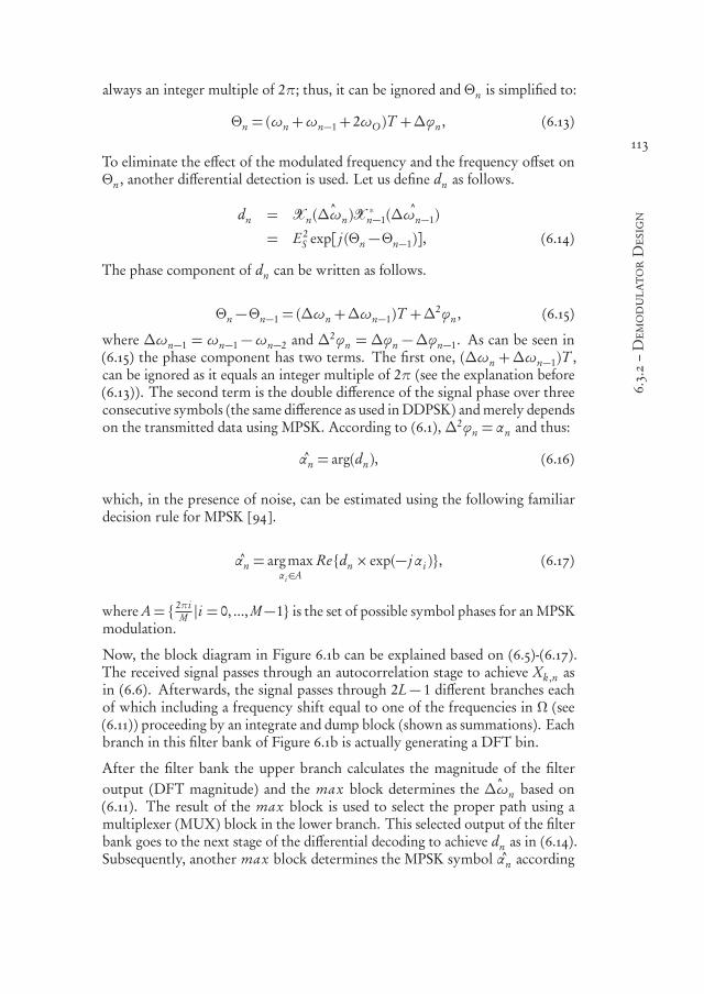
550999-L-bw-Siavash550999-L-bw-Siavash550999-L-bw-Siavash550999-L-bw-SiavashProcessed on: 23-11-2020Processed on: 23-11-2020Processed on: 23-11-2020Processed on: 23-11-2020 PDF page: 135PDF page: 135PDF page: 135PDF page: 135
113
6.3.2–DemodulatorDesign
always an integer multiple of 2π; thus, it can be ignored and Θn is simplified to:
Θn = (ωn +ωn−1+ 2ωO )T +∆ϕn , (6.13)
To eliminate the effect of the modulated frequency and the frequency offset onΘn , another differential detection is used. Let us define dn as follows.
dn = Xn( ˆ∆ωn)X∗n−1( ˆ∆ωn−1)
= E2S exp[ j (Θn −Θn−1)], (6.14)
The phase component of dn can be written as follows.
Θn −Θn−1 = (∆ωn +∆ωn−1)T +∆2ϕn , (6.15)
where ∆ωn−1 = ωn−1 −ωn−2 and ∆2ϕn = ∆ϕn −∆ϕn−1. As can be seen in(6.15) the phase component has two terms. The first one, (∆ωn +∆ωn−1)T ,can be ignored as it equals an integer multiple of 2π (see the explanation before(6.13)). The second term is the double difference of the signal phase over threeconsecutive symbols (the same difference as used inDDPSK) andmerely dependson the transmitted data using MPSK. According to (6.1), ∆2ϕn = αn and thus:
αn = arg(dn), (6.16)
which, in the presence of noise, can be estimated using the following familiardecision rule for MPSK [94].
αn = argmaxαi∈A
Redn × exp(− jαi ), (6.17)
where A= 2πiM |i = 0, ..., M−1 is the set of possible symbol phases for anMPSK
modulation.
Now, the block diagram in Figure 6.1b can be explained based on (6.5)-(6.17).The received signal passes through an autocorrelation stage to achieve Xk ,n asin (6.6). Afterwards, the signal passes through 2L− 1 different branches eachof which including a frequency shift equal to one of the frequencies in Ω (see(6.11)) proceeding by an integrate and dump block (shown as summations). Eachbranch in this filter bank of Figure 6.1b is actually generating a DFT bin.
After the filter bank the upper branch calculates the magnitude of the filteroutput (DFT magnitude) and the max block determines the ˆ∆ωn based on(6.11). The result of the max block is used to select the proper path using amultiplexer (MUX) block in the lower branch. This selected output of the filterbank goes to the next stage of the differential decoding to achieve dn as in (6.14).Subsequently, another max block determines the MPSK symbol αn according

550999-L-bw-Siavash550999-L-bw-Siavash550999-L-bw-Siavash550999-L-bw-SiavashProcessed on: 23-11-2020Processed on: 23-11-2020Processed on: 23-11-2020Processed on: 23-11-2020 PDF page: 136PDF page: 136PDF page: 136PDF page: 136
114
Chapter6–HybridModulationandTimeDiversity
Figure 6.2: The relation between signal bandwidth (BS ), sampling frequency(Fs ), filter bandwidth (BF ) and maximum tolerable frequency offset ( fO,max )
to (6.17). Finally, the detected symbols using phase and frequency are demappedto achieve the initial bits transmitted using MPSK and LFSK modulations.
It is worth mentioning that the branches in the filter bank add much less com-plexity compared to the DFT. The middle branch corresponding to∆ωn = 0 in-cludes only additions. Furthermore, the multiplication factors for the frequencyshift in the lower half of the branches in Figure 6.1b, are complex conjugates ofthe upper half. This means that the values of the multiplications in the upperhalf can be reused for the lower one as well. Thus, for LFSK only L−1 branchesinclude complex multiplications.
6.3.3 Tolerable Frequency Offset
As shown above, the effect of frequency offset on the frequency and the phase ofthe received signal is removed from corresponding decision variables (see (6.6)and (6.15), respectively). So in principle, the derived demodulator performsindependent of the frequency offset. The main parameter which determines thefrequency offset tolerance is the bandwidth of the low-pass filter prior to thedemodulator (see Figure 6.1b).
Similar to what discussed in Chapter 3, a filter with bandwidth equal to BF asshown in Figure 6.2 is assumed. The sampling frequency (for complex samples)is set to Fs = 2BF . Bt represents the transition band of the filter which is notzero for practical filters. The signal bandwidth (null-to-null) and the maximumtolerable frequency offset are shown by BS and ± fO,max , respectively.
In Chapter 3 (section 3.5.1), it was shown that, for Bt = 0, the range of themaximum tolerable frequency offset normalized to the symbol rate is (see (3.26)):
−N −BS/RS
2≤
fO
RS≤+
N −BS/RS
2(6.18)

550999-L-bw-Siavash550999-L-bw-Siavash550999-L-bw-Siavash550999-L-bw-SiavashProcessed on: 23-11-2020Processed on: 23-11-2020Processed on: 23-11-2020Processed on: 23-11-2020 PDF page: 137PDF page: 137PDF page: 137PDF page: 137
115
6.4–TheProposedDemodulatorinaTime-VaryingChannel
For hybrid modulation, the signal bandwidth, BS , is mainly determined by thebandwidth of the FSK modulation [34]. For the proposed modulator/demodu-lator, the bandwidth of LFSK can be approximated (null-to-null) as follows [103](notice that a rectangular pulse is used).
BS = (L− 1) fs e p + 2RS (6.19)
where fs e p and RS are the frequency separation of the FSK modulation and thesymbol rate, respectively. In the proposed system, fs e p = RS which simplifiesthe signal bandwidth approximation to BS = (L+1)RS . Consequently, the rangeof the tolerable frequency offset normalized to the symbol rate is:
− N − L− 12
≤fO
RS≤+N − L− 1
2(6.20)
For any L, the frequency offset tolerance of the proposed demodulator onlydepends on N (which is determined by the filter bandwidth) and can be modifiedby increasing the bandwidth of the filter prior to the demodulator as well as thesampling frequency.
6.4 The Proposed Demodulator in a Time-Varying Chan-
nel
One motivation for hybrid modulation is a higher power efficiency comparedto higher order PSK. On the other hand, the offset tolerant demodulator targetsUNB applications which are vulnerable to temporal fading due to their longsymbol period. This raises the question whether using the hybrid method withthe proposed demodulator instead of higher orders of PSK has benefits when atime-varying channel is considered. To answer this question, the performanceof the hybrid demodulator is analyzed in a time-varying fading channel.
The improvement of hybrid modulation in an AWGN channel and a flat fadingand time-invariant Rayleigh channel has been analytically shown in literature[16, 34, 35, 57]. However, to the best of our knowledge the performance ofhybrid modulation in a time-varying channel has not been investigated. A time-varying channel also called frequency dispersive channel, is encountered wheneither the transceivers move or transceivers are fixed but the surrounding objects(scatterers) move. It implies that the received signal has a randomly varyingphase and amplitude. The time varying phase is translated to a random frequencymodulation which distorts the signal and leads to an error even for SN R=∞[71]. This irreducible error is called, error floor, in this work.
In [36], the performance of simple receivers for FSK and PSK is consideredin a time-varying channel for low data rate applications. It is shown that, incontrast with DPSK, non-coherent FSK does not suffer from an error floor intime-varying channels. This property makes non-coherent FSK an attractive
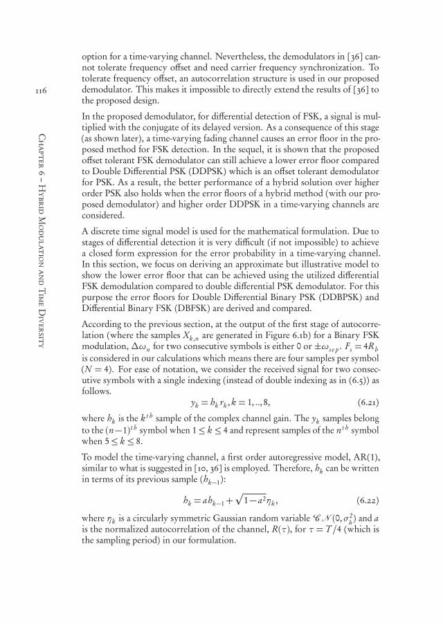
550999-L-bw-Siavash550999-L-bw-Siavash550999-L-bw-Siavash550999-L-bw-SiavashProcessed on: 23-11-2020Processed on: 23-11-2020Processed on: 23-11-2020Processed on: 23-11-2020 PDF page: 138PDF page: 138PDF page: 138PDF page: 138
116
Chapter6–HybridModulationandTimeDiversity
option for a time-varying channel. Nevertheless, the demodulators in [36] can-not tolerate frequency offset and need carrier frequency synchronization. Totolerate frequency offset, an autocorrelation structure is used in our proposeddemodulator. This makes it impossible to directly extend the results of [36] tothe proposed design.
In the proposed demodulator, for differential detection of FSK, a signal is mul-tiplied with the conjugate of its delayed version. As a consequence of this stage(as shown later), a time-varying fading channel causes an error floor in the pro-posed method for FSK detection. In the sequel, it is shown that the proposedoffset tolerant FSK demodulator can still achieve a lower error floor comparedto Double Differential PSK (DDPSK) which is an offset tolerant demodulatorfor PSK. As a result, the better performance of a hybrid solution over higherorder PSK also holds when the error floors of a hybrid method (with our pro-posed demodulator) and higher order DDPSK in a time-varying channels areconsidered.
A discrete time signal model is used for the mathematical formulation. Due tostages of differential detection it is very difficult (if not impossible) to achievea closed form expression for the error probability in a time-varying channel.In this section, we focus on deriving an approximate but illustrative model toshow the lower error floor that can be achieved using the utilized differentialFSK demodulation compared to double differential PSK demodulator. For thispurpose the error floors for Double Differential Binary PSK (DDBPSK) andDifferential Binary FSK (DBFSK) are derived and compared.
According to the previous section, at the output of the first stage of autocorre-lation (where the samples Xk ,n are generated in Figure 6.1b) for a Binary FSKmodulation, ∆ωn for two consecutive symbols is either 0 or ±ωs e p . Fs = 4Rbis considered in our calculations which means there are four samples per symbol(N = 4). For ease of notation, we consider the received signal for two consec-utive symbols with a single indexing (instead of double indexing as in (6.5)) asfollows.
yk = hk rk , k = 1, .., 8, (6.21)
where hk is the k t h sample of the complex channel gain. The yk samples belongto the (n−1)t h symbol when 1≤ k ≤ 4 and represent samples of the n t h symbolwhen 5≤ k ≤ 8.
To model the time-varying channel, a first order autoregressive model, AR(1),similar to what is suggested in [10, 36] is employed. Therefore, hk can be writtenin terms of its previous sample (hk−1 ):
hk = ahk−1+p
1− a2ηk , (6.22)
where ηk is a circularly symmetric Gaussian random variable CN (0,σ2h ) and a
is the normalized autocorrelation of the channel, R(τ), for τ = T /4 (which isthe sampling period) in our formulation.

550999-L-bw-Siavash550999-L-bw-Siavash550999-L-bw-Siavash550999-L-bw-SiavashProcessed on: 23-11-2020Processed on: 23-11-2020Processed on: 23-11-2020Processed on: 23-11-2020 PDF page: 139PDF page: 139PDF page: 139PDF page: 139
117
6.4–TheProposedDemodulatorinaTime-VaryingChannel
Let H = [h1, h2, ..., h8] denote the vector including all eight samples of the chan-nel gain over two consecutive symbols. Denoting the first element by h1 = hand applying (6.22) recursively, element hm of H (for m = 2,3, .., 8) is obtainedin terms of h.
H (m) = hm = am−1h +m−1∑
i=1
a i−1p
1− a2ηm−i , (6.23)
The output of the first stage of the demodulator can be calculated as follows(k = 1, ..., 4):
Yk = yk+4y∗k = hk+4 rk+4h∗k r ∗k (6.24)
Substituting hk from (6.23) into (6.24) and ignoring terms including ηiη j , weachieve the following equations for Yk , k = 1, .., 4:
Yk = a2(k+1)|h|2Xk + ak+3k−1∑
i=1
a i−1p
1− a2hη∗k−i Xk
+ak−1k+3∑
i=1
a i−1p
1− a2h∗ηk+4−i Xk , (6.25)
where Xk = rk+4 r ∗k and k = 1, ..., 4.
From (6.25) it can be seen that Yk includes random terms in addition to thesignal component which is a consequence of random variables ηi . Hereafter, forerror floor calculations, the random terms including ηi are called distortion andthe ratio of signal power to the power of these random terms is referred to asSDR (Signal to Distortion Ratio).
Considering Binary FSK in Figure 6.1b, Yk passes through three branches offiltering to achieve F−1, F0 and F+1 which are filter bank outputs correspondingto −ωs e p , 0 and +ωs e p , respectively. Due to the Xk component in all distortionterms and the correlation between random terms in samples of Yk (resultingfrom the recursive nature of the channel model), the distortion power is not thesame at the output of all filters.
The distortion caused by a time-varying channel manifests itself as a random vari-able with a non-uniform power spectral density. The main part of the distortionpower is concentrated in the filter matched to the signal frequency (Xn( ˆ∆ωn))and the amount of distortion power in the adjacent filters is much smaller. Incase the signal is at e.g. F+1, the distortion power in the non-adjacent filter (F−1 )is even negligible.
Based on this distortion, the error probability for BFSK is calculated. Since theGaussian (receiver) noise is assumed to be zero, this error probability provides uswith an error floor. The frequency component of Xk in (6.25) is either∆ωn = 0

550999-L-bw-Siavash550999-L-bw-Siavash550999-L-bw-Siavash550999-L-bw-SiavashProcessed on: 23-11-2020Processed on: 23-11-2020Processed on: 23-11-2020Processed on: 23-11-2020 PDF page: 140PDF page: 140PDF page: 140PDF page: 140
118
Chapter6–HybridModulationandTimeDiversity
or ∆ωn = ±ωs e p . When ∆ωn = 0 the error occurs if either |F+1| > |F0| or|F−1|> |F0|. On the other hand, when ∆ωn is +ωs e p or −ωs e p , the error hap-pens if |F0|> |F+1| or |F0|> |F−1|, respectively. ∆ωn is zero if two consecutiveBFSK symbols are the same; which has a probability of 1/2. If symbols aredifferent,∆ωn will be either+ωs e p or−ωs e p with a probability of 1/4 for each.Therefore, the probability of error is as follows:
Pe ,BF SK = 0.5[P (|F+1|> |F0|
∆ωn = 0)
+P (|F−1|> |F0|
∆ωn = 0)]
+0.25P (|F0|> |F−1|
∆ωn =−ωd )
+0.25P (|F0|> |F+1|
∆ωn =+ωd ) (6.26)
Each error probability in (6.26) is similar to the error probability for non-coherent BFSK when a matched filter (correlation) based demodulator is used[45]. However, there is a significant difference that must be taken into account.The conventional error probability function of non-coherent BFSK (based onmatched filters [45]) is derived based on the assumption of equal noise powerdensity in all filters which is not the case here. This problem can be solvedby calculating the noise power in the matched filter and the adjacent filter andrecalculate the error probabilities using the modified noise power for each filter.Each individual term in (6.26) is in the form of P (|Fx |> |Fy |) (where Fx and Fyare adjacent filters) conditioned on the fact that the signal is in Fy . Therefore,the derivation of all the probabilities in (6.26) are the same and the mathematicalderivation is continued for Pe = P (|F+1|> |F0|
∆ωn = 0).
According to the demodulator structure in Figure 6.1b, and in case ∆ωn = 0, F0and F+1 can be written as follows.
F0 =4∑
k=1
Yk =p
PS e− j∆ϕn +Æ
PN ,0ηT0 (6.27)
F+1 =4∑
k=1
Yk e− j (∆ωs e p kTs ) ≈Æ
PN ,+1ηT1 (6.28)
where ηT0 and ηT
1 are CN (0,1), e− j∆ϕn denotes the modulated phase and ES/Nis considered to be one without loss of generality. PS , PN ,0 and PN ,+1 are asfollows.
PS = S(a)|h|4 (6.29)PN ,0 = Υ0(a)|h|
2σ2h (1− a2) (6.30)
PN ,+1 = Υ+1(a)|h|2σ2
h (1− a2) (6.31)

550999-L-bw-Siavash550999-L-bw-Siavash550999-L-bw-Siavash550999-L-bw-SiavashProcessed on: 23-11-2020Processed on: 23-11-2020Processed on: 23-11-2020Processed on: 23-11-2020 PDF page: 141PDF page: 141PDF page: 141PDF page: 141
119
6.4–TheProposedDemodulatorinaTime-VaryingChannel
where S(a), Υ0(a) and Υ+1(a) are functions of a which is J0(2πυmax T /4) for aRayleigh fading channel with a Jakes spectrum and a maximum Doppler shift ofυmax . To simplify notations, in the following, S(a), Υ0(a) and Υ+1(a) are shownby S , Υ0 and Υ+1, respectively. The process of deriving (6.27)-(6.31) and detailedexpressions are presented in Appendix C.
P (|F+1| > |F0|
∆ωn = 0) (denoted by Pe in the following) can be written asfollows [45].
Pe =∫ +∞
0P (|F+1|> |F0|
|F0|) f|F0|(|F0|)d |F0| (6.32)
where f|F0|(|F0|) is the probability density function (pdf) of |F0| when ∆ωn = 0.Notice that the signal component of F+1 is negligible and is ignored in (6.28).Since ηT
1 ∼ CN (0,1), it is concluded that F+1 ∼ CN (0, PN ,+1). Hence, |F+1|has a Rayleigh distribution with σ2 = PN ,+1/2. Thus, we have:
P (|F+1|> |F0|
|F0|) =∫ ∞
|F0|fF1(x)d x = exp(
−|F0|2
Pn,+1) (6.33)
where fF1(x) is the pdf of |F+1| (when ∆ωn = 0) as follows.
fF1(x) =
2xPN ,+1
exp(− x2
PN ,+1), x ≥ 0 (6.34)
Substituting (6.33) into (6.32), using values in (6.29)-(6.31) and following a proce-dure similar to calculations in [45] (equations (7.231)-(7.243)) for non-coherentorthogonal modulations, the following equation for the error probability canbe obtained.
Pe =PN ,+1
PN ,+1+ PN ,0exp(−
PS
PN ,+1+ PN ,0) (6.35)
Substituting PS , PN ,0 and PN ,+1 from (6.29)-(6.31) we have:
Pe =Υ+1
Υ+1+Υ0exp(−
S |h|2
(Υ+1+Υ0)(1− a2)σ2h
) (6.36)
Now, we have the error probability which depends on |h|2. To achieve the aver-age error probability we need to integrate it over |h|2. For each set of three sym-bols, h is a Gaussian complex random variable h ∼CN (0,σ2
h ) according to thedefinition of a Rayleigh channel. Thus, it is concluded that |h| ∼Rayleigh(σ2
h/2)

550999-L-bw-Siavash550999-L-bw-Siavash550999-L-bw-Siavash550999-L-bw-SiavashProcessed on: 23-11-2020Processed on: 23-11-2020Processed on: 23-11-2020Processed on: 23-11-2020 PDF page: 142PDF page: 142PDF page: 142PDF page: 142
120
Chapter6–HybridModulationandTimeDiversity
and |h|2 ∼Exp(1/σ2h ) where Exp is the exponential distribution with the follow-
ing pdf:
f (x) =1σ2
h
exp(− xσ2
h
), x ≥ 0 (6.37)
Replacing |h|2 with x in (6.36) and using (6.37), the average error probability Peis achieved as follows [97].
Pe =∫ ∞
0Pe (x) f (x)d x
=(1− a2)Υ+1
(1− a2)(Υ0+Υ+1)+ S(6.38)
As mentioned earlier, each individual probability in (6.26) is derived using thesame process and their values are the same. Thus, the error floor (EFDBF SK ) isobtained by replacing each probability term in (6.26) with Pe from (6.38).
EFDBF SK =32
(1− a2)Υ+1
(1− a2)(Υ0+Υ+1)+ S(6.39)
Now, we need to calculate the error floor for DDBPSK. In a DDBPSK demod-ulator, the signal after the first stage is equal to F0 which is used as the input ofthe second stage. According to (6.27), F0 has a signal component and a Gaussiannoise (distortion) component. It can be seen as a signal with an SNR equal toPS/PN ,0. Since for DDBPSK, the second stage is simply differential detection ofantipodal symbols, the error probability is derived as follows [97].
Pe ,DP SK =12
1
1+ SN R, (6.40)
To calculate the error floor, it is assumed that there is no receiver noise (AWGN).As mentioned earlier, the Gaussian random variables in the above equations area consequence of time-variation of the channel. Thus, instead of SNR in (6.40),we may use the term, SDR (Signal to Distortion Ration), which is as follows.
SDR=PS
PN ,0=
S |h|2
Υ0(1− a2)σ2h
(6.41)
Considering the pdf of |h|2 as in (6.37) and integrating over |h|2, the averageSDR is:

550999-L-bw-Siavash550999-L-bw-Siavash550999-L-bw-Siavash550999-L-bw-SiavashProcessed on: 23-11-2020Processed on: 23-11-2020Processed on: 23-11-2020Processed on: 23-11-2020 PDF page: 143PDF page: 143PDF page: 143PDF page: 143
121
6.5–SystemDesignforTimeDiversity
SDR=S
Υ0(1− a2)(6.42)
Substituting (6.42) into (6.40), the error floor for DDBPSK is achieved as follows.
EFDDBP SK =Υ0(1− a2)
2Υ0(1− a2)+ 2S, (6.43)
Figure 6.3 demonstrates the error floor for different values of the maximumDoppler shift in a Rayleigh fading channel with a Jakes Doppler spectrum. Solidlines show values obtained from (6.39) and (6.43) while dashed lines are simu-lation results. It can be seen that the theoretical and simulation results are inagreement while there is a slight difference for the higher values of υmax . In ourapproximations the multiplication of noise terms is ignored. This assumptiondoes not hold for large values of Doppler shift which increases the variance ofthe random component in (6.22). Thus, as υmax increases, the theory slightlydeviates from simulations. Figure 6.3 demonstrates that the error floor achievedby DBFSK using the proposed demodulator is lower than the one that can beobtained by the conventional DDBPSK. Increasing the modulation order ofDDPSK is equivalent to using a higher order DPSK for which the input signalis modeled as (6.27). This leads to even higher error. As a result, if modulationorder is increased by combining DLFSK and DDPSK, the error floor is expectedto be lower compared to the error floor achieved when increasing the order ofDDPSK.
6.5 System Design for Time Diversity
In UNB communications, the proposed offset tolerant demodulator can be uti-lized to increase the bit-rate and employ channel coding and interleaving so thatthe time diversity which is provided by a time-varying channel is exploited.
In a general case of using time diversity, a system similar to Figure 6.4a can beemployed. First, information bits are sent to the channel encoder. Then, aninterleaver is used to make sure that the coded bits belonging to one codewordare distributed in time and experience different channel fading conditions. Inthe next step, the sequence of bits is split into two sets; BP SK and BF SK . Theformer set is modulated using MPSK and the latter is sent using LFSK. The bitsin BP SK and BF SK are modulated using the hybrid modulator and transmitted.After passing through the channel and adding AWGN noise, the samples of thesignal enter the demodulator. The output of the demodulator is fed to the Mixand De-Interleave block which puts the two sets of the detected bits together anddeinterleaves them. In the last step, the channel decoder uses the detected anddeinterleaved bits to extract information bits. In the block diagram of Figure6.4a any channel coding can be used.

550999-L-bw-Siavash550999-L-bw-Siavash550999-L-bw-Siavash550999-L-bw-SiavashProcessed on: 23-11-2020Processed on: 23-11-2020Processed on: 23-11-2020Processed on: 23-11-2020 PDF page: 144PDF page: 144PDF page: 144PDF page: 144
122
Chapter6–HybridModulationandTimeDiversity
0.01 0.03 0.05 0.07 0.09 0.11 0.13 0.15 0.17 0.1910−5
10−4
10−3
10−2
10−1
100
υmaxT
ErrorFloor
DBFSK Theory
DBFSK Sim
DDBPSK Theory
DDBPSK Sim
Figure 6.3: Simulated and theoretical error floor versus normalized maximumDoppler shift in a Rayleigh fading channel with Jakes Doppler spectrum
In this work we focus on the simplest form of channel coding which is repetitioncoding. Assuming a packet of information bits, the increased bit-rate is used tore-transmit the information packet several times during the same packet-timethat is needed for BFSK (2FSK) or BPSK (2PSK) modulation to transmit thesame set of information bits. Figure 6.4b and Figure 6.4c show the scheme usedin the dashed box A of Figure 6.4a. Notice that hybrid LFSK/MPSKmodulationmakes it possible to transmit log2(M )+log2(L) replicas of the information bits inthe same packet time. Another way of increasing the bit-rate is using higher orderDDPSK (DDMPSK). In the following sections, the BER performance of hybridmodulation is compared to different orders of DDMPSK. Using only DDMPSKthe number of replicas is log2(M ) (see Figure 6.4b). Figure 6.4c visualizes howthe bits in each replica of information packet are split between BF SK and BP SK .
In case of temporal fading, the replicas transmitted at different time instancesexperience different channel fading and making decisions considering these in-stances will improve the BER performance. In the system shown in Figure 6.4a,in a general case, the bits of a codeword (which are interleaved and split in time)are de-interleaved after demodulation and detection. For a repetition codingscheme, an option for the decoder is majority voting. For each information bit,voting over various detected replicas determines the final value. However, in thisway all replicas have an equal effect on the final decision regardless of their cor-responding instantaneous SNR. Including the effect of the instantaneous SNRvalue decreases the probability of error in the final decision. Assume that the

550999-L-bw-Siavash550999-L-bw-Siavash550999-L-bw-Siavash550999-L-bw-SiavashProcessed on: 23-11-2020Processed on: 23-11-2020Processed on: 23-11-2020Processed on: 23-11-2020 PDF page: 145PDF page: 145PDF page: 145PDF page: 145
123
6.5–SystemDesignforTimeDiversity
Info
Pack
et
Hyb
rid
Mod
ulat
orC
hann
el
Enc
oder
Inte
rlea
ve&
Spl
it
Hyb
rid
Dem
odul
ator
Cha
nnel
D
ecod
er
Mix
&
De-
Inte
rlea
ve
Channel
Info
Pack
et
A B
(a)
tT
x P
acke
tT
x P
acke
tT
x P
acke
t
Tx
Pac
ket w
itho
ut ti
me
dive
rsit
y (B
FS
K o
r B
PS
K)
Hig
her
Bit
Rat
e (h
ybri
d (L
FS
K/M
PS
K)
or M
PS
K)
+ T
ime
dive
rsity
No
Tim
e di
vers
ity
Num
ber
of tr
ansm
itte
d re
plic
as:
Tx
Pac
ket
(b)
Info
Pac
ket
Info
Pac
ket
Info
Pac
ket
Info
Pac
ket
(c)
Bip
olar
Con
vers
ion
Bip
olar
Con
vers
ion
Mix & De-Interleave
Info
Pack
et
(d)
Figure
6.4:Blockdiagram
ofa)
thedesig
nedsystem
fortim
ediversity
,b)distribu
tionof
thereplicas
ofinform
ationpacket,c
)splittin
ginform
ationbitsto
B FSK
and
B PSK,and
d)thedecoderfor
repetitioncoding
includ
ingtheeffecto
finstantaneous
SNR.
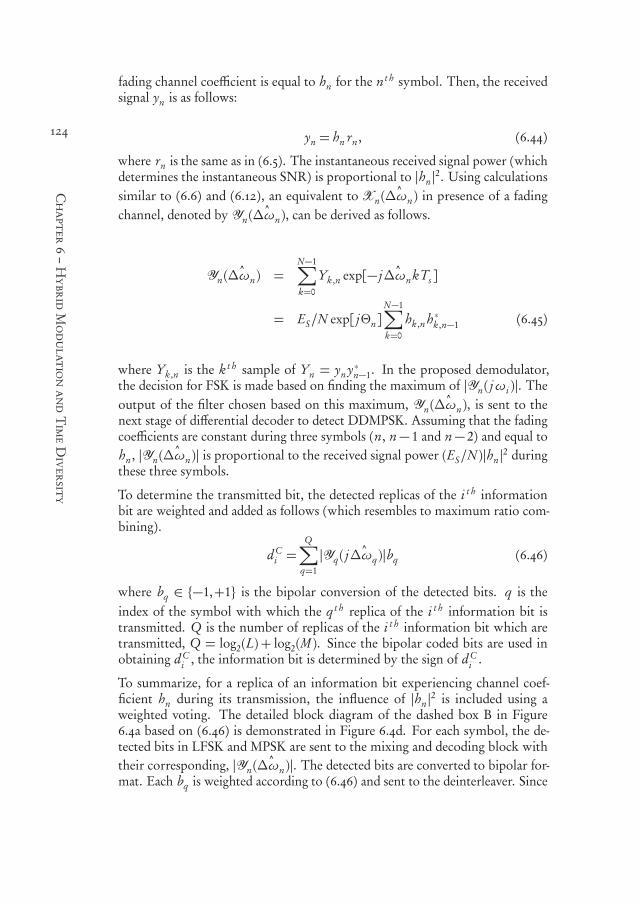
550999-L-bw-Siavash550999-L-bw-Siavash550999-L-bw-Siavash550999-L-bw-SiavashProcessed on: 23-11-2020Processed on: 23-11-2020Processed on: 23-11-2020Processed on: 23-11-2020 PDF page: 146PDF page: 146PDF page: 146PDF page: 146
124
Chapter6–HybridModulationandTimeDiversity
fading channel coefficient is equal to hn for the n t h symbol. Then, the receivedsignal yn is as follows:
yn = hn rn , (6.44)
where rn is the same as in (6.5). The instantaneous received signal power (whichdetermines the instantaneous SNR) is proportional to |hn |2. Using calculationssimilar to (6.6) and (6.12), an equivalent to Xn( ˆ∆ωn) in presence of a fadingchannel, denoted by Yn( ˆ∆ωn), can be derived as follows.
Yn( ˆ∆ωn) =N−1∑
k=0
Yk ,n exp[− j ˆ∆ωn kTs ]
= ES/N exp[ jΘn]N−1∑
k=0
hk ,n h∗k ,n−1 (6.45)
where Yk ,n is the k t h sample of Yn = yn y∗n−1. In the proposed demodulator,the decision for FSK is made based on finding the maximum of |Yn( jωi )|. Theoutput of the filter chosen based on this maximum, Yn( ˆ∆ωn), is sent to thenext stage of differential decoder to detect DDMPSK. Assuming that the fadingcoefficients are constant during three symbols (n, n− 1 and n− 2) and equal tohn , |Yn( ˆ∆ωn)| is proportional to the received signal power (ES/N )|hn |2 duringthese three symbols.
To determine the transmitted bit, the detected replicas of the i t h informationbit are weighted and added as follows (which resembles to maximum ratio com-bining).
d Ci =
Q∑
q=1
|Yq ( j ˆ∆ωq )|bq (6.46)
where bq ∈ −1,+1 is the bipolar conversion of the detected bits. q is theindex of the symbol with which the q t h replica of the i t h information bit istransmitted. Q is the number of replicas of the i t h information bit which aretransmitted, Q = log2(L) + log2(M ). Since the bipolar coded bits are used inobtaining d C
i , the information bit is determined by the sign of d Ci .
To summarize, for a replica of an information bit experiencing channel coef-ficient hn during its transmission, the influence of |hn |2 is included using aweighted voting. The detailed block diagram of the dashed box B in Figure6.4a based on (6.46) is demonstrated in Figure 6.4d. For each symbol, the de-tected bits in LFSK and MPSK are sent to the mixing and decoding block withtheir corresponding, |Yn( ˆ∆ωn)|. The detected bits are converted to bipolar for-mat. Each bq is weighted according to (6.46) and sent to the deinterleaver. Since
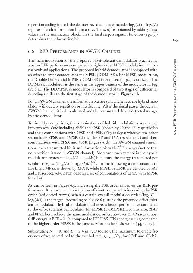
550999-L-bw-Siavash550999-L-bw-Siavash550999-L-bw-Siavash550999-L-bw-SiavashProcessed on: 23-11-2020Processed on: 23-11-2020Processed on: 23-11-2020Processed on: 23-11-2020 PDF page: 147PDF page: 147PDF page: 147PDF page: 147
125
6.6–BERPerformanceinAWGN
Channel
repetition coding is used, the de-interleaved sequence includes log2(M )+ log2(L)replicas of each information bit in a row. Thus, d C
i is obtained by adding thesevalues in the summation block. In the final step, a signum function ( s g n(.))determines the information bit.
6.6 BER Performance in AWGN Channel
The main motivation for the proposed offset-tolerant demodulator is achievinga better BER performance compared to higher order MPSK modulation in ultra-narrowband applications. The proposed hybrid demodulator is compared withan offset tolerant demodulator for MPSK (DDMPSK). For MPSK modulation,the Double Differential MPSK (DDMPSK) introduced in [94] is utilized. TheDDMPSK modulator is the same as the upper branch of the modulator in Fig-ure 6.1a. The DDMPSK demodulator is composed of two stages of differentialdecoding similar to the first stage of the demodulator in Figure 6.1b.
For an AWGN channel, the information bits are split and sent to the hybrid mod-ulator without any repetition or interleaving. After the signal passes through anAWGN channel, it is demodulated and the transmitted data is detected using ahybrid demodulator.
To simplify comparison, the combinations of hybrid modulations are dividedinto two sets. One including 2PSK and 4PSK (shown by 2P and 2F, respectively)and their combinations with 2FSK and 4FSK (Figure 6.5a); whereas, the otherset includes 8PSK and 16PSK (shown by 8P and 16P, respectively) and theircombinations with 2FSK and 4FSK (Figure 6.5b). In AWGN channel simula-tions, each transmitted bit is an information bit with E I n f
b energy (notice thatno repetition is used in AWGN channel). Moreover, each symbol in the hybridmodulation represents log2(L)+ log2(M ) bits; thus, the energy transmitted persymbol is ES = (log2(L) + log2(M ))E
I n fb . In the following a combination of
LFSK and MPSK is shown by LFMP, while MPSK or LFSK are denoted by MPand LF, respectively. LFxP denotes a set of combinations of LFSK with MPSKfor all M .
As can be seen in Figure 6.5, increasing the FSK order improves the BER per-formance. It is also much more power efficient compared to increasing the PSKorder (red dotted curves) when a certain overall modulation order ( log2(L) +log2(M )) is the target. According to Figure 6.5, using the proposed offset toler-ant demodulator, hybrid modulation achieves a better performance comparedto the offset tolerant demodulator for MPSK (DDMPSK). For instance, 2F4Pand 8PSK both achieve the same modulation order; however, 2F4P saves almost6 dB energy at BER=0.1% compared to DD8PSK. This energy saving comparedto the higher order MPSK is the same as what has been shown in [34, 52, 57].
Substituting N = 10 and L = 2,4 in (3.25)-(6.20), the maximum tolerable fre-quency offset normalized to the symbol rate, fO,max/RS , for 2FxP and 4FxP is

550999-L-bw-Siavash550999-L-bw-Siavash550999-L-bw-Siavash550999-L-bw-SiavashProcessed on: 23-11-2020Processed on: 23-11-2020Processed on: 23-11-2020Processed on: 23-11-2020 PDF page: 148PDF page: 148PDF page: 148PDF page: 148
126
Chapter6–HybridModulationandTimeDiversity
6 8 10 12 14 16 1810−6
10−5
10−4
10−3
10−2
10−1
100
EInfb
/N0[dB]
BER
2P
2F2P
4F2P
4P
2F4P
4F4P
(a)
6 8 10 12 14 16 1810−6
10−5
10−4
10−3
10−2
10−1
100
EInfb
/N0[dB]
BER
8P
2F8P
4F8P
16P
2F16P
4F16P
(b)
Figure 6.5: BER curves for hybrid modulation in an AWGN channel for combi-nation of 2FSK and 4FSK with a) 2PSK and 4PSK, b) 8PSK and 16PSK

550999-L-bw-Siavash550999-L-bw-Siavash550999-L-bw-Siavash550999-L-bw-SiavashProcessed on: 23-11-2020Processed on: 23-11-2020Processed on: 23-11-2020Processed on: 23-11-2020 PDF page: 149PDF page: 149PDF page: 149PDF page: 149
127
6.7–BERPerformanceinaTime-VaryingChannel
−500 −300 −100 100 300 50010−4
10−3
10−2
10−1
100
fO
BER
2F4P
4F4P
Figure 6.6: BER performance of hybrid modulation for 2F4P and 4F4P. Aninverse-sinc low-pass filter (see Figure 6.1b) is used with Bt = 100 Hz and BF = 1kHz while RS = 100 Sym./s and Fs = 1 kHz
3.5 and 2.5, respectively. The ability of the proposed demodulator to toleratefrequency offset is demonstrated in Figure 6.6 where BER values for 2F4P and4F4P at Eb/N0 = 12 dB can be seen when −500 Hz< fO <+500 Hz. To showthe effect of the filter frequency response on the offset tolerance, an inverse-sinclow-pass filter is considered with Bt ≈ 100 Hz and BF = 500 Hz. The symbolrate is 100 Sym./s and Fs = 1 kHz. As can be seen the BER is constant for| fO |< 250 Hz and fO < 150 Hz, in case of 2F4P and 4F4P, respectively. Thesevalues are 100Hz less than the expected values which is a consequence of nonzeroBt equal to 100 Hz. The increase in the BER for a larger frequency offset is nota consequence of the demodulator characteristics but due to lack of coverage bythe filter. To solve this, a wider filter can be used and the sampling frequencymust increase accordingly.
6.7 BER Performance in a Time-Varying Channel
To configure the system and perform comparisons, a few assumptions, criteriaand definitions are introduced. This is necessary to clarify further discussionsand guarantee a fair comparison. These are summarized as follows:
1. It is assumed that a constant number of information bits is required tobe transmitted denoted by T X I n f .

550999-L-bw-Siavash550999-L-bw-Siavash550999-L-bw-Siavash550999-L-bw-SiavashProcessed on: 23-11-2020Processed on: 23-11-2020Processed on: 23-11-2020Processed on: 23-11-2020 PDF page: 150PDF page: 150PDF page: 150PDF page: 150
128
Chapter6–HybridModulationandTimeDiversity
2. A reference symbol rate, RRe fS , is defined as a baseline. This is equal to
the information bit-rate RI n fb in case of a simple 2PSK transmission.
3. A reference packet time, T Re fP , is defined. The packet time in this simplest
case (2PSK) is the time needed to send T X I n f information bits with asymbol rate equal to RRe f
S . The symbol rate is equal to the bit-rate in thissimplest case. The target is to keep T Re f
P constant as it determines the RFcircuit power consumption which is a significant contributor to the nodepower consumption. As a result, transmitting more bits for redundancyjust by prolonging the overall transmission time is not included in thiscomparison as it is considered not to be efficient.
4. A constant energy per information bit is considered as E I n fb . The target is
to improve performance without increasing the energy transmitted per in-formation bit. In other words, redundant information is sent with lowerenergy to make sure that the overall transmitted energy per informationbit remains constant. This affects the energy per transmitted symbolwhich is discussed further for each scenario.
5. Higher order PSK and the hybrid modulation scheme are used to increasethe raw bit-rate and transmit redundant information for time diversity.Since in this work we use repetition coding, Repetition Order (RO) isdefined as the ratio of the achieved raw bit-rate and RRe f
S . This is, in fact,the inverse of the code rate. For instance, 2PSK has a repetition orderof 1 and a combination of 2FSK and 4PSK (shown by 2F4P) provides arepetition order of 3 (1 from 2FSK and 2 from 4PSK).
In our simulations, T X I n f equals 240 which is in the same order of short packetlengths used in UNB applications [2, 55]. Besides, it is divisible by the repetitionorders achieved using hybrid combinations and higher order MPSK which arediscussed here. This makes the analysis easier and more straightforward withoutloss of generality. The reference symbol rate RRe f
S is equal to 100 Sym./s whichis also the same as in [2, 55]. This makes T Re f
P equal to 2.4 s. The rest ofthe scenarios and parameters are built up according to this baseline. In eachapplication, these parameters can be set accordingly. Then, the insight providedby the following results can be used to understand the trade-offs and choose thebest modulation scheme.
The Rayleigh fading (with Jakes spectrum) channel is considered as the worstcase channel. A popular application for UNB communication is fixed wirelesslinks. In these links the transmitter and the receiver nodes are static and thetemporal fading is caused by movement of the scatterers (such as cars, peopleand foliage in the wind). Several measurement campaigns and a large amountof research has been performed to model the channel in such applications indifferent environments [5, 40, 51, 77] (though they do not specifically considerUNB). Elaborating on the channel models and their analysis in fixed wireless

550999-L-bw-Siavash550999-L-bw-Siavash550999-L-bw-Siavash550999-L-bw-SiavashProcessed on: 23-11-2020Processed on: 23-11-2020Processed on: 23-11-2020Processed on: 23-11-2020 PDF page: 151PDF page: 151PDF page: 151PDF page: 151
129
6.7.1–ConstantSymbolRateScenario
links is not in the scope of this thesis. Nevertheless, to illustrate the performanceof the proposed method in different channel characteristics, simulation resultsfor a more realistic channel model in fixed wireless scenarios are presented as well.According to [28, 77], in a fixed wireless link, the channel model is more similarto Rician channel and the Doppler shift has a higher distribution density aroundzero. Hence, a more realistic channel model is a Rician channel with a roundedDoppler spectrum rather than a Rayleigh channel with the Jakes spectrum ofwhich simulation results will also be presented [28].
The error floor analysis in the previous section was performed for the worstcase which is a Rayleigh channel. The BER performance for both Rayleigh andRician channel based on simulations will be presented in the following. TheK-factor in a Rician channel depends on several parameters. In our simulations,for the Rician channel, we have considered K = 1 which means that the powerof the line-of-sight component is equal to the power summed over the multipathcomponents. Furthermore, in the scenarios with the highest Doppler spreadconsidered for a fixed wireless channel in [28], the maximum Doppler shiftis around 2 Hz. To show the effect of a higher maximum Doppler shift, theproposed demodulator is also evaluated for Dmax = 5 Hz. In a time-invariantchannel, using time-diversity does not lead to improvement as it does not add anydiversity; therefore, the results for a time-invariant channel are not presented.
For MPSK, four different values of M are considered (M = 2,4,8,16). This set ofmodulation orders will clearly show the intended trade-offs. For LFSK, L= 2,4are considered since small L-values impose lower bandwidth overhead. Thesevalues for M and L form eight different combinations for hybrid modulationwhich are analyzed in the simulations. The number of samples per symbol isconsidered to be N = 10. Table 6.2 summarizes the basic simulation parameters.
As mentioned earlier, increasing the raw bit-rate, in an efficient way, is a motiva-tion for hybrid modulation. For MPSK modulation, the ratio of the raw bit-rateto RRe f
S , what we defined as repetition order (RO), is equal to log2(M ). Forhybrid modulation composed of LFSK and MPSK, this repetition order equals:
RO = log2(L)+ log2(M ) (6.47)
Table 6.3 demonstrates the combinations and the repetition order which can beachieved using them. In the following subsections, two different scenarios areconsidered for evaluating hybrid modulation in a time-varying fading channel;constant symbol rate and equal bandwidth.
6.7.1 Constant Symbol Rate Scenario
The symbol rate of a communication link determines the effect of a time-varyingchannel on the BER performance. In fact, the severity of the temporal fadingdepends on the maximumDoppler shift normalized to the symbol rate (Dmax T )

550999-L-bw-Siavash550999-L-bw-Siavash550999-L-bw-Siavash550999-L-bw-SiavashProcessed on: 23-11-2020Processed on: 23-11-2020Processed on: 23-11-2020Processed on: 23-11-2020 PDF page: 152PDF page: 152PDF page: 152PDF page: 152
130
Chapter6–HybridModulationandTimeDiversity
Table 6.2: Simulation parameters
T XI n f 240
RRe fS 100
T Re fP [s] 2.4
Maximum Doppler shift (Dmax ) [Hz] 2,5
K factor for Rician channel 1
N (Sam p l e/Sy mb ol ) 10
L 2,4
M 2,4,8,16
Table 6.3: Different combinations and the corresponding repetition order
No FSK 2FSK 4FSK
No PSK - 1 2
2PSK 1 2 3
4PSK 2 3 4
8PSK 3 4 5
16PSK 4 5 6
[71]. Therefore, to keep the effect of temporal fading constant for comparison,the symbol rate is maintained constant in this scenario. Since the bandwidthusage in UNB communications is not critical, it is reasonable to assume that thebandwidth increase due to using FSK modulation can be afforded. The higherrepetition order achieved by hybrid modulation or higher order DDMPSK isused for adding time diversity with repetition coding using the system in Figure6.4.
As the symbol rate and packet time (the third criterion mentioned at the begin-ning of this section) are constant in this scenario, the number of symbols thatare transmitted remains constant and equal to T X I n f . For any modulation inTable 6.3, the repetition order (RO ) shows the number of replicas that can betransmitted for each information bit. Based on the fourth criterion, the E I n f
b
is kept constant which requires E I n fb to be distributed over all redundant bits.
As a result, energy per transmitted bit, Eb , is E I n fb /RO. Finally, each symbol
includes RO bits so the energy per transmitted symbol in our scenario is equalto the energy per information bit.
For a better performance, error correcting codes are usually used instead of sim-ple repetition coding. Hence, the interesting part of the BER curve without errorcorrection code is around BER= 0.1%. To provide an overview, the E I n f
b /N0
550999-L-bw-Siavash550999-L-bw-Siavash550999-L-bw-Siavash550999-L-bw-SiavashProcessed on: 23-11-2020Processed on: 23-11-2020Processed on: 23-11-2020Processed on: 23-11-2020 PDF page: 153PDF page: 153PDF page: 153PDF page: 153
131
6.7.2–EqualBandwidthScenario
required for BER= 0.1% for Rayleigh and Rician channels and Dmax = 2, 5 Hzare shown in Figure 6.7 (the BER curves for different combinations and channelmodels can be found in Appendix D). The horizontal axis shows the order ofPSK modulation. Each bar represents stand alone PSK (red), PSK in combina-tion with 2FSK (blue) and PSK in combination with 4FSK (green). When thePSK order equals 1 (the leftmost bars in Figure 6.7), there is no phase modula-tion so these cases refer to pure FSK modulation. The bars hit the maximumof the vertical axis when the error floor is higher than BER = 0.1% (i.e. theynever reach BER= 0.1%). It is clearly seen that 4PSK performs the best whencombinations with FSK (blue and green bars) are considered. Furthermore, in-creasing FSK order improves performance for all PSK orders. It is also seen thatfor hybrid modulation, 4 is the best choice for PSK order. It increases diversitybut degrades BER performance less significantly compared to 8PSK and 16PSK.
6.7.2 Equal Bandwidth Scenario
The improvement in the BER performance of hybrid modulation, compared toDDMPSK, is obtained at the expense of higher bandwidth usage. Increase inbandwidth is not prohibitive in UNB applications; that is why, in the previoussubsection, it is not considered in comparisons. To include different bandwidthusage of these two modulations in our evaluation, an equal bandwidth scenariois also investigated.
In this scenario the bandwidth of the hybrid modulation is considered as thereference and the symbol rate of the DDMPSK is changed such that it occupiesthe same bandwidth as the hybrid method. Then, the modulations with equalbandwidth are compared (they may achieve different repetition orders while oc-cupying the same bandwidth). According to (6.19) from section 6.3, for a symbolrate equal to RRe f
S = 100 Sym./s, combining 2FSK and 4FSK with MPSK (2FxPand 4FxP), the null-to-null bandwidths become 3RRe f
S and 5RRe fS , respectively.
MPSK modulation with a null-to-null bandwidth equal to 3RRe fS and 5RRe f
S canhave a symbol rate equal to 1.5RRe f
S and 2.5RRe fS , respectively (notice that a
rectangular pulse shape is assumed and, therefore, PSK null-to-null bandwidth istwice the symbol rate). Using these higher symbol rates for MPSK, the numberof transmitted symbols during T Re f
P is increased and this can be used to transmitredundant information in the same packet time.
So starting from a given PSK modulation scheme, the repetition order can beincreased in two ways:
1. FSK in combination with PSK: It increases the bandwidth of the signal andthe repetition order (symbol rate remains RRe f
S ).2. MPSK with higher symbol rate (fast MPSK): This means that the raw bit-
rate is increased and more bits can be transmitted during T Re fP . This also
increases bandwidth.

550999-L-bw-Siavash550999-L-bw-Siavash550999-L-bw-Siavash550999-L-bw-SiavashProcessed on: 23-11-2020Processed on: 23-11-2020Processed on: 23-11-2020Processed on: 23-11-2020 PDF page: 154PDF page: 154PDF page: 154PDF page: 154
132
Chapter6–HybridModulationandTimeDiversity
1 2 4 8 1615
20
25
30
35
40
PSK Order
Eb/N
0forBER
=0.1%
[dB]
No FSK2F4F
(a) Rayleigh with Dmax = 2 H z
1 2 4 8 1615
20
25
30
35
40
PSK Order
Eb/N
0forBER
=0.1%
[dB]
No FSK2F4F
(b) Rayleigh with Dmax = 5 H z
1 2 4 8 1615
20
25
30
35
40
PSK Order
Eb/N
0forBER
=0.1%
[dB]
No FSK2F4F
(c) Rice with K = 1 and Dmax = 2 H z
1 2 4 8 1615
20
25
30
35
40
PSK Order
Eb/N
0forBER
=0.1%
[dB]
No FSK2F4F
(d) Rice withK = 1 and Dmax = 5 H z
Figure 6.7: E I n fb /N0 required for BER= 0.1% in constant symbol rate scenario.
The channel model is Rayleigh with Jakes Doppler spectrum for (a) and (b).The channel model is Rice with K = 1 and Rounded Doppler spectrum for (c)and (d). The horizontal axis is the order of PSK and order equal to 1 meansthere is only FSK modulation.
With a symbol rate equal to RS for an MPSK modulated signal, the total numberof transmitted symbols (T XSy m ) during the reference packet time (T Re f
P ) andthe achieved RO are as follows.
T XSy m = T XI n f × (RS/RRe fS ) (6.48)
RO =T XSy m × log2(M )
T XI n f= log2(M )× (RS/RRe f
S ) (6.49)

550999-L-bw-Siavash550999-L-bw-Siavash550999-L-bw-Siavash550999-L-bw-SiavashProcessed on: 23-11-2020Processed on: 23-11-2020Processed on: 23-11-2020Processed on: 23-11-2020 PDF page: 155PDF page: 155PDF page: 155PDF page: 155
133
6.7.2–EqualBandwidthScenario
2 4 815
20
25
30
35
PSK Order
Eb/N
0forBER
=0.1%
[dB]
2F1.5Rs
4F2.5Rs
(a) Rayleigh with Dmax = 2 H z
2 4 815
20
25
30
35
PSK Order
Eb/N
0forBER
=0.1%
[dB]
2F1.5Rs
4F2.5Rs
(b) Rayleigh with Dmax = 5 H z
2 4 815
20
25
30
35
PSK Order
Eb/N
0forBER
=0.1%
[dB]
2F1.5Rs
4F2.5Rs
(c) Rice with K = 1 and Dmax = 2 H z
2 4 815
20
25
30
35
PSK Order
Eb/N
0forBER
=0.1%
[dB]
2F1.5Rs
4F2.5Rs
(d) Rice withK = 1 and Dmax = 5 H z
Figure 6.8: E I n fb /N0 required for BER= 0.1% in equal bandwidth scenario. The
channel model is Rayleigh with Jakes Doppler spectrum for (a) and (b). Thechannel model is Rice with K = 1 and Rounded Doppler spectrum for (c) and(d). The horizontal axis is the order of PSK.
Remember that the symbol rate for FPSK remains RRe fS and the repetition order
is achieved using (6.47). Different combinations of LFSK and MPSK as well asdifferent combinations of MPSK with higher symbol rates are shown in Table6.4. The value in each cell of the table shows the repetition order that can beachieved with the corresponding combination.
For hybrid modulations in this scenario, the symbol rate does not change andwill be the same as RRe f
S . So a constant packet time (assumption 3) meansthat the number of symbols that are transmitted remains constant and equalto T X I n f . To determine energy per transmitted symbol, similar reasoning asfor constant symbol rate scenario can be used for the hybrid modulation in theequal bandwidth scenario. Thus, energy per transmitted bit Eb , is E I n f
b /RO andenergy per transmitted symbol (for hybrid modulation) is E I n f
b .
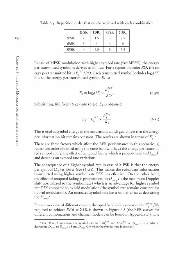
550999-L-bw-Siavash550999-L-bw-Siavash550999-L-bw-Siavash550999-L-bw-SiavashProcessed on: 23-11-2020Processed on: 23-11-2020Processed on: 23-11-2020Processed on: 23-11-2020 PDF page: 156PDF page: 156PDF page: 156PDF page: 156
134
Chapter6–HybridModulationandTimeDiversity
Table 6.4: Repetition order that can be achieved with each combination
2FSK 1.5RS 4FSK 2.5RS
2PSK 2 1.5 3 2.5
4PSK 3 3 4 5
8PSK 4 4.5 5 7.5
In case of MPSK modulation with higher symbol rate (fast MPSK), the energyper transmitted symbol is derived as follows. For a repetition order RO, the en-ergy per transmitted bit is E I n f
b /RO. Each transmitted symbol includes log2(M )bits so the energy per transmitted symbol ES is:
ES = log2(M )×E I n f
b
RO, (6.50)
Substituting RO from (6.49) into (6.50), ES is obtained.
ES = E I n fb ×
RRe fS
RS(6.51)
This is used as symbol energy in the simulations which guarantees that the energyper information bit remains constant. The results are shown in terms of E I n f
b .
There are three factors which affect the BER performance in this scenario; 1)repetition order obtained using the same bandwidth, 2) the energy per transmit-ted symbol and 3) the effect of temporal fading which is proportional to Dmax Tand depends on symbol rate variations.
The consequence of a higher symbol rate in case of MPSK is that the energyper symbol (ES ) is lower (see (6.51)). This makes the redundant informationtransmitted using higher symbol rate PSK less effective. On the other hand,the effect of temporal fading is proportional to Dmax T (the maximum Dopplershift normalized to the symbol rate) which is an advantage for higher symbolrate PSK compared to hybrid modulation (the symbol rate remains constant forhybrid modulation). An increased symbol rate has a similar effect as decreasingthe Dmax
1.
For an overview of different cases in the equal bandwidth scenario, the E I n fb /N0
required to achieve BER = 0.1% is shown in Figure 6.8 (the BER curves fordifferent combinations and channel models can be found in Appendix D). The
1The effect of increasing the symbol rate to 1.5RRe fS and 2.5RRe f
S on Dmax T is similar todecreasing Dmax to Dmax/1.5 and Dmax/2.5 when the symbol rate is constant.

550999-L-bw-Siavash550999-L-bw-Siavash550999-L-bw-Siavash550999-L-bw-SiavashProcessed on: 23-11-2020Processed on: 23-11-2020Processed on: 23-11-2020Processed on: 23-11-2020 PDF page: 157PDF page: 157PDF page: 157PDF page: 157
135
6.8–Conclusion
horizontal axis in the diagrams shows the PSK order while each bar shows eitherthe combination of that PSK order with FSK (blue and green bars) or usingsolely PSK with a higher symbol rate (red and orange bars). Similar to theconstant symbol rate scenario, 4PSK performs the best among all PSK orders.Furthermore, a combination with FSK needs less E I n f
b /N0 compared to fast PSKin case of equal bandwidth occupation. The difference is not large in a Rayleighchannel and particularly for combinations with 2FSK; however, it grows when acombination with 4FSK or a Rician channel are considered. Similar to the con-stant symbol rate scenario, among the considered combinations, 4F4P performsthe best with (at least) around 2 dB improvement compared to 2.5RS MPSK.
6.8 Conclusion
The effects of a time-varying channel in combination with Carrier FrequencyOffset (CFO) were considered simultaneously for ultra-narrowband (UNB) com-munications. An offset tolerant demodulator was proposed for a general case ofhybrid LFSK/MPSK modulation using Differential LFSK and Double Differen-tial MPSK (DDMPSK). Hybrid modulation increases the raw bit-rate in a morepower efficient manner compared to higher order MPSK. The increased bit-ratecan be exploited by introducing channel coding and diversity techniques to im-prove the performance of a UNB system in time-varying fading channels. Thehigher bit-rate achieved by hybrid modulation was used for a simple repetition ofthe information packet during the same packet time. The system was simulatedin Rayleigh and Rician channels with maximum Doppler shifts equal to 2 Hzand 5 Hz. The BER performance of the proposed demodulator was comparedwith an offset tolerant Double Differential MPSK demodulator in different sce-narios. It was shown that at BER=0.1%, a hybrid modulation scheme performsbetter than the MPSK modulation in all cases by at least 1 dB and up to morethan 10 dB depending on the modulation order, scenario, channel model andmaximum Doppler shift. Using a simple repetition coding and time diversity,a combination of 4FSK and 4PSK (4F4P) is the best combination among theinvestigated modulations. Considering all cases, 4F4P requires 2 dB less Eb/N0than the best DDMPSK at BER=0.1%. In this work, repetition coding was usedfor its simplicity. The BER performance and complexity trade-offs, when usingother coding schemes, requires further study. Moreover, using the proposedhybrid demodulator in combination with frequency diversity is an interestingdirection for future research.

550999-L-bw-Siavash550999-L-bw-Siavash550999-L-bw-Siavash550999-L-bw-SiavashProcessed on: 23-11-2020Processed on: 23-11-2020Processed on: 23-11-2020Processed on: 23-11-2020 PDF page: 158PDF page: 158PDF page: 158PDF page: 158
136

550999-L-bw-Siavash550999-L-bw-Siavash550999-L-bw-Siavash550999-L-bw-SiavashProcessed on: 23-11-2020Processed on: 23-11-2020Processed on: 23-11-2020Processed on: 23-11-2020 PDF page: 159PDF page: 159PDF page: 159PDF page: 159
1377Conclusion
Low Power Wide Area Networks (LPWANs) are an emerging type of wirelessnetworks which realize long range and low data rate communication for IoT ap-plications. Ultra-Narrowband (UNB) communication is one of the interestingtechnologies for implementation of LPWAN. It uses unlicensed spectrum, offersrobustness against interference and provides low cost communication with awide coverage. Although the very low data rate in UNB communication relaxessome aspects of the transceiver design (such as lower clock frequencies in the base-band processing), it poses other challenges. The extremely narrow bandwidth ofthe signal in UNB communications (in the order of a few hundred hertz) makesUNB susceptible to Carrier Frequency Offset (CFO) and temporal fading.
Amismatch between the transmitter and the receiver oscillators or themovementof the transceiver nodes relative to each other can cause CFO. Offset tolerantdemodulators have been proposed in literature as a solution to the problemof CFO and as an alternative for precise but power hungry carrier frequencyrecovery. However, most of these methods are designed for cases where thefrequency offset is in the order of the signal bandwidth or even smaller than that.Such a value for CFO in a UNB communication system requires very precisecrystals with thermal compensation which are not cost and energy efficient.
Temporal fading is the variation of the channel during transmission time. Thechallenge of a time-varying fading channel is more severe for UNB communica-tion due to their long symbol periods and transmission times. Even if wirelessnodes are fixed, which is usually the case for the UNB communication sys-tems, movement of the scatterers of the signal (surrounding objects) leads to atime-varying channel. Time and frequency diversity techniques combined withchannel coding and interleaving can be utilized to improve the reliability of thecommunication in a time-varying fading channel. Nevertheless, these schemesrequire transmitting redundant bits which makes the transmission time in aUNB system even longer.
This thesis focused on addressing the above mentioned challenges in the down-
550999-L-bw-Siavash550999-L-bw-Siavash550999-L-bw-Siavash550999-L-bw-SiavashProcessed on: 23-11-2020Processed on: 23-11-2020Processed on: 23-11-2020Processed on: 23-11-2020 PDF page: 160PDF page: 160PDF page: 160PDF page: 160
138
Chapter7–Conclusion
link of a UNB system using offset tolerant demodulators. This chapter summa-rizes the contributions and presents some possible directions for future research.First, in the next section the contributions are summarized and the researchquestions introduced in Chapter 1 are answered. Then, recommendations forfuture research are proposed for further investigation.
7.1 Summary
7.1.1 Offset Tolerant Demodulators for UNB
As mentioned earlier, most of the offset tolerant demodulators assume that theCFO is in the order of the signal bandwidth or even smaller. In case of UNBcommunication, such a CFO still needs high precision carrier recovery andcostly crystals. Therefore, to combat the CFO while using low cost crystalsand avoiding high precision carrier recovery, offset tolerant demodulators forUNB need to tolerate very large frequency offsets. That is why the first researchquestion presented in Chapter 1 was defined as follows.
1. What are the limitations of offset tolerant demodulators, which can toleratelarge frequency offset, for UNB communications?
The answer to this question is sought in Chapter 3 where we considered twodifferent modulation schemes that are mostly used in UNB communications,namely, FSK and PSK. The goal was to investigate demodulators which cantolerate arbitrarily large frequency offsets given that the low-pass filter beforethe demodulator captures the signal properly in the presence of CFO. The BERperformance and the complexity of the two demodulators were investigated tofind out their limitations when large CFO tolerance is required.
Among various FSK demodulators, a demodulator based on the Discrete FourierTransform (DFT) was selected as the one with potential to tolerate large fre-quency offset. Therefore, a DFT-based demodulator was designed for BFSKusing a simple detection algorithm. An existing DFT-based window synchro-nization scheme was used for the DFT-based demodulator. This synchronizationscheme is necessary to tolerate large frequency offset and in our design it is alsoused to determine the bins of the DFT corresponding to the transmitted BFSKfrequencies.
For PSKmodulation an autocorrelation based demodulator (ACD) was used. Us-ing Double Differential encoding for PSK and ACD as demodulator, the decisionmetric will be independent of the frequency offset value; thus, a Double Differ-ential PSK signal can be detected in the presence of a relatively large frequencyoffset (multiple time the symbol rate). To have a fair comparison between thecomplexity of the FSK and PSK demodulators, a synchronization algorithm wasdesigned and used for PSK which is independent of the frequency offset.
The BER performance of these two demodulators, when a large offset toleranceis needed, were evaluated. In the presence of a large CFO, a wide low-pass filter

550999-L-bw-Siavash550999-L-bw-Siavash550999-L-bw-Siavash550999-L-bw-SiavashProcessed on: 23-11-2020Processed on: 23-11-2020Processed on: 23-11-2020Processed on: 23-11-2020 PDF page: 161PDF page: 161PDF page: 161PDF page: 161
139
7.1.2–ScalableOffsetTolerance
is required prior to the demodulators so that the signal can be captured. Thisincreases the noise power at the input of the demodulator. It was shown that theBER performance of DDPSK degrades as a consequence of the increased noisepower. The simulation results showed that the Eb/N0 required for BER= 0.1%increases by 2 dB when the range of tolerable offset changes from around ±3RSto ±15RS (N = 8 and N = 32). In contrast, the BER performance of the DFT-based demodulator is not affected by the bandwidth of the low-pass filter. For theDFT-based demodulator the DFT works as a filter bank. Since the number ofDFT points increases when the tolerable offset increases, the bandwidth of eachof these filters remains constant independent of the filter before the demodulator.Thus, the BER performance of the DFT-based demodulator does not change.
The complexity of the two demodulators was calculated in terms of complexmultiplications and additions required for synchronization and symbol detection.It was shown that the complexity of the DDPSK increases linearly with thenumber of samples per symbol, N . On the other hand, the complexity of theDFT-based demodulator is in the order of N 2 log2(N ) which is considerablylarger than the complexity of the DDPSK demodulator. The number of samplesper symbol is proportional to the range of tolerable frequency offset; therefore,when the range of tolerable frequency offset increases, the complexity of theDFT-based demodulator increases drastically. As an example, the complexityof the DFT-based demodulator for each symbol detection (assuming a packetlength of 250 symbols) becomes 20 times larger when the range of tolerableoffset changes from ±3RS to ±15RS (N = 8 and N = 32).
The simulation results and discussions showed that a DDPSK demodulator islimited by its BER performance degradation while the DFT-based demodulatorcan lead to a drastic increase of complexity when the range of offset toleranceincreases. To enable large offset tolerance, these limitations need to be overcome.
7.1.2 Scalable Offset Tolerance
The scalable offset tolerance was introduced as one of the main targets of thiswork. As defined in Chapter 2, scalable offset tolerancemeans achieving the sameBER performance for a certain Eb/N0 independent of the CFO. According tothe previous subsection, the investigated offset tolerant demodulators for PSKand FSK both have limitations in presence of arbitrarily large frequency offset.The BER performance of the DDPSK demodulator degrades when a large offsettolerance is required. On the other hand, the complexity of the DFT-baseddemodulator extremely increases if a larger offset tolerance is required. Theselimitations raised the second research question:
2. How can we circumvent the limitations of the demodulators to achievescalable offset-tolerance?
The solutions for demodulator limitations were discussed in Chapter 4 and Chap-ter 5 and are summarized in the following.

550999-L-bw-Siavash550999-L-bw-Siavash550999-L-bw-Siavash550999-L-bw-SiavashProcessed on: 23-11-2020Processed on: 23-11-2020Processed on: 23-11-2020Processed on: 23-11-2020 PDF page: 162PDF page: 162PDF page: 162PDF page: 162
140
Chapter7–Conclusion
Shifted correlation for DDPSK
In Chapter 4, the BER performance of the autocorrelation demodulator (ACD)for DDPSK in the presence of a large frequency offset was considered. AlthoughDDPSK is able to tolerate frequency offset, the wide filter required for a large off-set tolerance includes more noise which leads to BER performance degradation.To find a solution, first, the problem was defined by investigating the ACD andthe noise distribution at its output. It was shown that the main reason for de-pendence of the BER performance on the filter bandwidth is the multiplicationof noise components in the first autocorrelation stage.
To overcome this problem, a shifted correlation method was proposed in Chap-ter 4. It is assumed that the sampling frequency at the output of the filter andthe input of the demodulator satisfies the Nyquist criterion with respect to thefilter bandwidth. Thus, when the filter is wider than the signal bandwidth thesymbols are oversampled. The proposed method exploits this oversampling byintroducing additional correlation paths to the conventional DDPSK demodula-tor. In each path, there are two stages similar to the conventional demodulator.In the first stage, the n t h symbol is correlated with a shifted version of the sam-ples of the (n − 1)t h symbol. The result of this stage passes through anotherdifferential decoder. The outputs of these paths are added together and this sumis used to make the final decision. As shown in Chapter 4, the proposed methodincreases the SNR at the input of the detector and compensates for the SNR lossresulting from the increased filter bandwidth. Therefore, the BER performanceremains almost unchanged for all values of the filter bandwidth. The simulationresults revealed that the proposed method leads to more than 2dB improvementin BER performance when the bandwidth of the filter is 16 times the symbolrate (which implies that the offset tolerance is around ±7RS ). For wider filtersi.e. wider range of frequency offset tolerance, this gain increases further.
Low complexity window synchronization for FSK
It was shown in Chapter 3 that the main drawback of the DFT-based offsettolerant demodulator is its complexity. The high complexity stems from thewindow synchronization algorithm which is used for this demodulator. Thewindow synchronization algorithm is necessary for the proper functioning ofthe demodulator; however, its complexity is prohibitive for tolerating a largefrequency offset. The existing synchronization algorithm for this demodulatoris complex as it involves calculating the DFT of a sliding window called SlidingDFT (SDFT).
A variety of algorithms have been proposed for efficient implementation of theSDFT. In our literature review in Chapter 5, these algorithms were divided intotwo categories, Complete SDFT (C-SDFT) and Single Bin SDFT (SB-SDFT).The former class computes all bins of the DFT altogether while the latter canbe used to calculate each bin separately. A review on the SDFT calculating
550999-L-bw-Siavash550999-L-bw-Siavash550999-L-bw-Siavash550999-L-bw-SiavashProcessed on: 23-11-2020Processed on: 23-11-2020Processed on: 23-11-2020Processed on: 23-11-2020 PDF page: 163PDF page: 163PDF page: 163PDF page: 163
141
7.1.3–OffsetToleranceandTemporalFading
structures in Chapter 5 showed that if the number of calculated bins of an N -point DFT is sufficiently small, the SDFT can be implemented efficiently usingSB-SDFT structure.
In light of these facts, a new synchronization algorithm was proposed where thenumber of the DFT bins required for synchronization is reduced. Actually, dueto zero-padding and oversampling, only a limited number of bins called the Binsof Interest (BoI) include signal information which is explained in Chapter 5. Tofind the BoI, a step-by-step zooming algorithm was proposed. Furthermore, theDFT-based demodulator introduced in Chapter 3, needs zero-padding for properperformance and the synchronization algorithm should also use zero paddingfor correct operation. However, existing SB-SDFT structures do not considerzero-padding. That is why a modified version of SB-SDFT was also proposed inChapter 5 to incorporate zero padding. The stability of the proposed SB-SDFTmethod was also considered and a stable version using a damping factor wasintroduced.
Using the proposed algorithm and its implementation based on the proposedSB-SDFT calculator, the complexity increases slower compared to the conven-tional synchronization algorithm when the range of tolerable CFO increases.It was shown that for an oversampling factor of eight the proposed algorithmobtains 68%, 48%, 61% saving in the number of complex additions, complexmultiplications and memory compared to the conventional synchronizationalgorithm while achieving the same BER performance. Based on simulationresults presented in Chapter 5, for an oversampling factor of 32, the numbers ofcomplex multiplications and complex additions are reduced by more than 85%(and memory more by 90%). This oversampling factor corresponds to an offsettolerance about ±14.5 times the symbol rate.
7.1.3 Offset Tolerance and Temporal Fading
As mentioned earlier in this chapter, temporal fading is another problem whichmust be considered in UNB communication. The third research question wasfocused on addressing CFO and temporal fading simultaneously.
3. How can we handle the temporal fading in UNB communication andachieve the required redundancy for diversity while using offset tolerant de-modulators?
Using diversity techniques is a solution to temporal fading; however, it requirestransmitting redundant information. Thus, we either need to increase the rawbit-rate or increase the transmission time. A longer transmission time meansthat the RF part is on for a longer time which increases power consumption.On the other hand, increasing the bit-rate using higher order PSK degrades theBER performance while using higher order FSK increases the bandwidth.
A third solution to increase the raw bit-rate is hybrid frequency/phase modu-lation which has been proposed in literature. It changes the power and band-

550999-L-bw-Siavash550999-L-bw-Siavash550999-L-bw-Siavash550999-L-bw-SiavashProcessed on: 23-11-2020Processed on: 23-11-2020Processed on: 23-11-2020Processed on: 23-11-2020 PDF page: 164PDF page: 164PDF page: 164PDF page: 164
142
Chapter7–Conclusion
width efficiency trade-off by providing more bandwidth efficiency than higherorder FSK and more power efficiency (from a BER performance perspective)compared to higher order PSK. The increased bit-rate can be exploited by intro-ducing channel coding and diversity techniques to improve the performance ofa UNB system in time-varying fading channels.
To tolerate CFO, an offset tolerant hybrid demodulator was proposed in chapter6. Different combinations of FSK and PSK orders were simulated using AWGNchannels. It was shown that for the combination of BFSK and QPSK, the pro-posed demodulator can achieve 6 dB improvement at BER= 0.1% compared toDD8PSK which provides the same modulation order (3 bits per symbol).
To alleviate the effect of temporal fading, a time diversity scheme was proposedusing the offset tolerant hybrid demodulator. The increased bit-rate achieved byhybrid modulation was used for re-transmitting the information bits during thesame packet time. The hybrid demodulator was simulated for different combi-nations of FSK and PSK. Rayleigh and Rician channel models were consideredwith maximum Doppler shifts equal to 2 Hz and 5 Hz. Two different scenarioswere considered for simulations: a constant symbol rate scenario and an equalbandwidth scenario.
It was shown that at BER= 0.1%, a hybrid modulation scheme performs betterthan higher order DDPSK modulation in all cases by at least 1 dB and up tomore than 10 dB depending on the modulation order, scenario, channel modeland maximum Doppler shift. Using simple repetition coding and time diversity,a combination of 4FSK and 4PSK (4F4P) is the best combination among theinvestigated modulations. Considering all cases, at BER = 0.1%, 4F4P needs2dB less E b/N0 than the best Double Differential MPSK.
7.2 Main Contributions
The main contributions of this thesis can be summarized as follows:
» We investigated the performance and complexity of two offset tolerantdemodulators for PSK and FSK which are capable of tolerating frequencyoffsets larger than the signal bandwidth. A DFT-based demodulator wasdesigned for FSK and an autocorrelation based double differential demod-ulator was considered for PSK. The evaluations clarified the limitations ofthese methods which were addressed in the rest of the work (Chapter 3).
» We developed and evaluated a shifted correlation scheme for DDPSKdemodulation. It alleviates the BER performance loss of the conventionalautocorrelation basedDDPSK demodulator in the presence of awide filterand large frequency offset (Chapter 4).
» We developed and evaluated a low complexity synchronization algorithmfor the DFT-based demodulator. This algorithm uses a subset of the DFTbins for synchronization. For efficient implementation of the proposed

550999-L-bw-Siavash550999-L-bw-Siavash550999-L-bw-Siavash550999-L-bw-SiavashProcessed on: 23-11-2020Processed on: 23-11-2020Processed on: 23-11-2020Processed on: 23-11-2020 PDF page: 165PDF page: 165PDF page: 165PDF page: 165
143
7.3–RecommendationsforFutureWork
synchronization algorithm a Single Bin Sliding DFT (SB-SDFT) structurewith zero-padding was designed as well (Chapter 5).
» We developed and evaluated an offset tolerant demodulator for hybrid fre-quency/phase modulation and designed a system based on time-diversityto overcome temporal fading. The hybrid modulation was utilized toincrease the raw bit-rate which was exploited to re-transmit the infor-mation packet during the same packet time. This system exploits thetime-diversity which is provided by a time-varying channel and improvesthe BER performance (Chapter 6).
7.3 Recommendations for Future Work
In this thesis, we mainly focused on a constant frequency offset. If the variationsin frequency offset remain sufficiently small, the proposed demodulator will notbe affected. For the DFT-based demodulator a variable CFO causes deviation ofFSK frequencies from the DFT bins determined during synchronization. Thesevariations can be tolerated as far as they remain smaller than the bin resolutionof the DFT during the whole packet. For DDPSK the variable offset can betolerated as far as the change in the CFO during three symbols remains negligible.For UNB applications a largely time-varying CFO is not very likely as thetransmitter and the receiver are mainly fixed. Nevertheless, it is interesting tolook for techniques to complement the proposed demodulators for low datarate applications where largely time-varying CFO exists. For the DFT-baseddemodulator, the adjacent bins of the bins selected in the synchronization phasecan bemonitored during the packet. In this way, using a decision directed scheme,if the adjacent bins have a higher average value during a few symbols, they canbe used as new bins for decision making. For the DDPSK, the linear variationin frequency offset shows itself as a constant phase at the output of the secondstage. To solve this, a decision directed method might be used to correct for thisphase offset and avoid performance loss.
As another solution for temporal fading, a frequency diversity technique can beused. It may use a hybrid modulation scheme and in addition to transmittingsignal over different time periods, it can transmit redundant information usingdifferent carrier frequencies (a sort of frequency hopping scheme). If the differ-ences between frequencies are selected carefully and are larger than the coherencebandwidth of the channel, this will add diversity and can improve performanceof the system. Although leveraging frequency diversity e.g. using frequencyhopping adds complexity, it is an interesting choice when the time variation ofa channel is too slow to provide the required diversity.
In the proposed scheme for temporal fading (Chapter 6), the repetition codingscheme was used. Although it offers considerable simplicity, its ability to im-prove performance is limited. It is anticipated that a better BER performancecan be achieved if a more complicated channel coding scheme is used. Since the
550999-L-bw-Siavash550999-L-bw-Siavash550999-L-bw-Siavash550999-L-bw-SiavashProcessed on: 23-11-2020Processed on: 23-11-2020Processed on: 23-11-2020Processed on: 23-11-2020 PDF page: 166PDF page: 166PDF page: 166PDF page: 166
144
Chapter7–Conclusion
processing power of the communication node in the downlink is limited, thetrade-off between the decoder complexity and the performance improvementmust be evaluated. On the other hand, the short packet length affects the perfor-mance of most channel coding schemes as they are usually optimized for longpackets. Finding a proper coding scheme for a short block length is an activeresearch topic in the field of Ultra-Reliable Low Latency (URLL) communi-cations for 5G. This formulates an interesting question for future research onfinding low code-rate and simple channel coding schemes which are suitable forthe proposed system.
In this work we focused on an offset tolerant demodulator and how it can handlefrequency offset in the physical layer. It would be interesting to look into theopportunities that such offset tolerant demodulators provide in the design of theMAC layer and network layer. In UNB communication systems such as Sigfox,the downlink communication is dependent on an uplink initiation. One of thereasons for this approach is the frequency uncertainty in the communicationnode. If an offset tolerant demodulator is used, the restrictions on the downlinkcommunication might be relaxed. On the other hand, if the fading problem canbe overcome efficiently using a diversity scheme (such as the one proposed inChapter 6), the reliability of the downlink communication in a UNB networkincreases. Nevertheless, figuring out how this can be exploited to improve theoverall capacity and/or reliability of a UNB network, needs further investigationof the MAC- and network layers.

550999-L-bw-Siavash550999-L-bw-Siavash550999-L-bw-Siavash550999-L-bw-SiavashProcessed on: 23-11-2020Processed on: 23-11-2020Processed on: 23-11-2020Processed on: 23-11-2020 PDF page: 167PDF page: 167PDF page: 167PDF page: 167
145

550999-L-bw-Siavash550999-L-bw-Siavash550999-L-bw-Siavash550999-L-bw-SiavashProcessed on: 23-11-2020Processed on: 23-11-2020Processed on: 23-11-2020Processed on: 23-11-2020 PDF page: 168PDF page: 168PDF page: 168PDF page: 168
146

550999-L-bw-Siavash550999-L-bw-Siavash550999-L-bw-Siavash550999-L-bw-SiavashProcessed on: 23-11-2020Processed on: 23-11-2020Processed on: 23-11-2020Processed on: 23-11-2020 PDF page: 169PDF page: 169PDF page: 169PDF page: 169
147AMathematical Proof for
kc Calculation Algorithm
According to the explanation in Chapter 5, to achieve kγc at each step, the magni-tudes of DFTs for a sliding window with 2N one-sample shifts are added. Then,kγc is the bin for which this sum has a maximum value (see (5.9) and (5.10)). Inthis appendix, it is mathematically shown that this sum over DFT magnitudeshas a maximum at the center frequency. This is correct as long as all the 2Nwindows are in the preamble. The first window can start in any part of either aone symbol or a zero symbol in the preamble.
As the zero-padding factor changes during the zoom stage, (5.9) and (5.10) mustbe shown for the general case of all zero-padding factors in different steps of thezooming algorithm. For this purpose the concept of the Discrete Time FourierTransform (DTFT) is used here. DTFT is a version of the Fourier Transformwhichmaps discrete time samples to a continuous frequency domain. TheDTFTof a discrete function in the time domain, shown by x[n], is denoted by X (Ω)where Ω= 2π f /Fs (−π<Ω<π) is the frequency normalized to the samplingfrequency, Fs . The k t h bin of the DFT calculated for N samples with zero-padding factor I , actually is the value X (Ω) of DTFT for effectively N samples,sampled at f = (k/N I )Fs (Ω= 2πk/N I ) [82]. Using the concept of the DTFT,(5.9) and (5.10) can be written as follows.
Ωc = maxΩ∈[−π.+π]
X (Ω) (A.1)
where:
X (Ω) =2N−1∑
i=0
|Xi (Ω)|2 (A.2)
Xi (Ω) is the DTFT for the i t h window and Ωc = 2π fc/Fs =ωc Ts . Because (A.1)and (A.2) are generalized versions of (5.9) and (5.10), which are true for all zero-
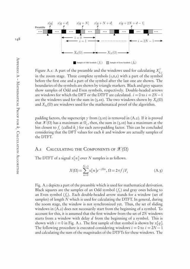
550999-L-bw-Siavash550999-L-bw-Siavash550999-L-bw-Siavash550999-L-bw-SiavashProcessed on: 23-11-2020Processed on: 23-11-2020Processed on: 23-11-2020Processed on: 23-11-2020 PDF page: 170PDF page: 170PDF page: 170PDF page: 170
148
AppendixA
–MathematicalProoffor
kcCalculationAlgorithm
Sample of Odd Symbols Sample of Even Symbols
Preamble
Figure A.1: A part of the preamble and the windows used for calculating X γk ,i
in the zoom stage. Three complete symbols (1,0,1) with a part of the symbolbefore the first one and a part of the symbol after the last one are shown. Theboundaries of the symbols are shown by triangle markers. Black and grey squaresshow samples of Odd and Even symbols, respectively. Double-headed arrowsare windows for which the DFT or the DTFT are calculated. i = 0 to i = 2N−1are the windows used for the sum in (5.10). The two windows shown by X0(Ω)and XN (Ω) are windows used for the mathematical proof of the algorithm.
padding factors, the superscript γ from (5.10) is removed in (A.2). If it is provedthatX (Ω) has a maximum at Ωc , then, the sum in (5.10) has a maximum at thebin closest to fc (called kc ) for each zero-padding factor. This can be concludedconsidering that the DFT values for each k and window are actually samples ofthe DTFT.
A.1 Calculating the Components ofX (Ω)
The DTFT of a signal x[n] over N samples is as follows.
X (Ω) =N−1∑
n=0
x[n]e− jΩn , Ω= 2π f /Fs (A.3)
Fig. A.1 depicts a part of the preamble which is used for mathematical derivation.Black squares are the samples of an Odd symbol ( f1 ) and gray ones belong toan Even symbol ( f0 ). Each double-headed arrow stands for a window (set ofsamples) of length N which is used for calculating the DTFT. In general, duringthe zoom stage, the window is not synchronized yet. Thus, the set of slidingwindows in (A.2) does not necessarily start from the beginning of a symbol. Toaccount for this, it is assumed that the first window from the set of 2N windowsstarts from a window with delay d from the beginning of a symbol. This isshown with i = 0 in Fig. A.1. The first sample of that symbol is shown by x[q].The following procedure is executed considering windows i = 0 to i = 2N − 1and calculating the sum of the magnitudes of the DTFTs for these windows. The

550999-L-bw-Siavash550999-L-bw-Siavash550999-L-bw-Siavash550999-L-bw-SiavashProcessed on: 23-11-2020Processed on: 23-11-2020Processed on: 23-11-2020Processed on: 23-11-2020 PDF page: 171PDF page: 171PDF page: 171PDF page: 171
149
A.1–CalculatingtheComponentsofX(Ω)
window i = 0 starts in an Odd symbol; nevertheless, the same mathematicalformulation can be achieved if the black and gray samples are interchanged in Fig.A.1 i.e. if i = 0 starts in an Even symbol. This generalization is possible becauseof the specific frequency separation for BFSK which is equal to the symbol rate.
Now, let us consider a pair of windows in the summation of (A.2) with delayd of the odd symbol ( f1 ) and the same delay for the next even symbol ( f0 ) (i.e.i = 0 and i =N in (A.2)). In Fig. A.1 these are shown by X0(Ω) and XN (Ω). IfG0(Ω) is defined as follows:
G0(Ω) = |X0(Ω)|2+ |XN (Ω)|
2 (A.4)
Then,X (Ω) can be derived in terms of N similar pairs and different Gm as:
X (Ω) =N−1∑
m=0
Gm(Ω) (A.5)
where Gm(Ω) = |Xm(Ω)|2+ |Xm+N (Ω)|2. First, G0(Ω) is analyzed. ConsideringBFSK modulation, the samples for the i = 0 and i =N window are as follows.
x0[n] =¨
e j (ω1(n+d+q)Ts ) 0≤ n <N − de j (ω0(n+d+q−N )Ts+θ1) N − d ≤ n <N
(A.6)
xN [n] =¨
e j (ω0(n+d+q)Ts+θ1) 0≤ n <N − de j (ω1(n+d+q−N )Ts+θ0+θ1) N − d ≤ n <N
(A.7)
where ω1 and ω0 are 2π f1 and 2π f0, respectively. In (A.6) and (A.7), θ1 =ω1NTs and θ0 =ω0NTs are actually accumulated phase at the end of an Oddsymbol and Even symbol, respectively. Without loss of generality, it is assumedthat the initial phase before x[q] (in Fig. A.1) is zero. Using x0[n], xN [n] andthe definition of the DTFT in (A.3), X0(Ω) and XN (Ω) are calculated.
X0(Ω) =N−d−1∑
n=0
e j (ω1Ts (n+d+q)−Ωn)
+N−1∑
n=N−d
e j (ω0Ts (n+d+q)−Ωn) (A.8)
XN (Ω) =N−d−1∑
n=0
e j (ω0Ts (n+d+q)+ω1N Ts−Ωn)
+N−1∑
n=N−d
e j (ω1Ts (n+d+q)+ω1N Ts−Ωn) (A.9)
550999-L-bw-Siavash550999-L-bw-Siavash550999-L-bw-Siavash550999-L-bw-SiavashProcessed on: 23-11-2020Processed on: 23-11-2020Processed on: 23-11-2020Processed on: 23-11-2020 PDF page: 172PDF page: 172PDF page: 172PDF page: 172
150
AppendixA
–MathematicalProoffor
kcCalculationAlgorithm
Notice that in (A.6) and (A.7), θ1−ω0NTs and θ0−ω1NTs are equal to+(ω1−ω0)NTs and −(ω1 −ω0)NTs , respectively. Remember from Chapter 3 andChapter 5 that the frequency separation of BFSK is equal to the symbol rateRSy m = 1/T and Ts/T = 1/N . So ±(ω1−ω0)NTs are removed from the phaseof the signals since they equal±2π. Now that the primary expressions for X0(Ω)and XN (Ω) are obtained, a new variable is introduced to simplify the rest of theproof.
A.2 Definition of α
The main target is to prove thatX (Ω) has a maximum at Ωc =ωc Ts . Since thefrequency separation of BFSK is equal to the symbol rate (1/T = 1/N Ts ),ω1Tsand ω0Ts can be written in terms of center frequency ωc as follows.
ω0Ts =ωc Ts −π/N , ω1Ts =ωc Ts +π/N , (A.10)
Now that ω0Ts and ω1Ts are written in the form of deviations from ωc Ts , letus define α as the deviation of Ω from Ωc .
α=Ω−ωc Ts (A.11)
In the following, the variableΩ is changed toωc Ts+α and (A.4), (A.5), (A.8) and(A.9) are formulated as functions of α. These new functions are denoted by a tildeover their name (for instanceX (Ω) changes to X (α)). When all functions areformulated in terms of α, instead of proving that there is a maximum at Ω=Ωc
forX (Ω), it must be proved that X (α) has a maximum at α= 0. This simplifiesthe calculations, particularly, it enables us to eliminate the terms related toωc Tswhich is seen in the expressions for ω1Ts and ω0Ts (A.10) as well.
By change of variable to α, (A.5) can be written as:
X (α) =N−1∑
m=0
Gm(α) (A.12)
For now, we focus on G0(α) = |X0(α)|2+ |XN (α)|2. Substitutingω1Ts andω0Tsfrom (A.10) to (A.8) and (A.9) while replacing Ω with ωc Ts +α we have:
X0(α) = e j (ωc Ts+πN )(d+q)
N−d−1∑
n=0
e j ( πN −α)n
+e j (ωc Ts−πN )(d+q)
N−1∑
n=N−d
e− j ( πN +α)n (A.13)

550999-L-bw-Siavash550999-L-bw-Siavash550999-L-bw-Siavash550999-L-bw-SiavashProcessed on: 23-11-2020Processed on: 23-11-2020Processed on: 23-11-2020Processed on: 23-11-2020 PDF page: 173PDF page: 173PDF page: 173PDF page: 173
151
A.2–Definitionofα
XN (α) = −e j [(ωc Ts−πN )(d+q)+ωc T ]
N−d−1∑
n=0
e j−( πN +α)n
−e j [(ωc Ts+πN )(d+q)+ωc T ]
N−1∑
n=N−d
e j ( πN −α)n (A.14)
where T = NTs and the terms which are independent of n are taken out ofsummation. As a result of the change of variable, π appears in the phase ofthe exponential functions in (A.9) which is converted to a negative sign beforethe summations in (A.14). For a complex function f (x), | f (x)|2 = f (x) f (x)∗
where f (x)∗ is the complex conjugate of f (x). Thus, the magnitudes of X0(α)and XN (α) are as follows.
|X0(α)|2 =
N−d−1∑
n, p=0
e j ( πN −α)(n−p)+d−1∑
n, p=0
e− j ( πN +α)(n−p)
+2N−d−1∑
n=0
N−1∑
p=N−d
cos(Θ(n, p)−α(n− p)) (A.15)
|XN (α)|2 =
N−d−1∑
n, p=0
e− j ( πN +α)(n−p)+d−1∑
n, p=0
e j ( πN −α)(n−p)
+2N−d−1∑
n=0
N−1∑
p=N−d
cos(−Θ(n, p)−α(n− p)) (A.16)
where Θ(n, p) = πN (2(d + q)+ n+ p) and the following equality is used:
M−1∑
m,k=0
am bk =M−1∑
m,k=0
ak bm =
M−1∑
m=0
am
M−1∑
m=0
bm
(A.17)
The first summation of (A.16) and the second summation of (A.15) can be rewrit-ten as follows.
A(α) =N−d−1∑
n, p=0
e− j ( πN +α)(n−p) =N−d−1∑
n, p=0
e j ( πN +α)(n−p) (A.18)
B(α) =d−1∑
n, p=0
e− j ( πN +α)(n−p) =d−1∑
n, p=0
e j ( πN +α)(n−p) (A.19)

550999-L-bw-Siavash550999-L-bw-Siavash550999-L-bw-Siavash550999-L-bw-SiavashProcessed on: 23-11-2020Processed on: 23-11-2020Processed on: 23-11-2020Processed on: 23-11-2020 PDF page: 174PDF page: 174PDF page: 174PDF page: 174
152
AppendixA
–MathematicalProoffor
kcCalculationAlgorithm
To obtain (A.18) and (A.19), first the negative sign before j is dissolved to (n− p)tomake (p−n); then, using a simple change of indexes in summation (see (A.17)),(p − n) is converted to (n− p). Also, using cos(x) = cos(−x), the third term of|XN (α)|2 can be written as follows.
C (α) = 2N−d−1∑
n=0
N−1∑
p=N−d
cos(Θ(n, p)+α(n− p)) (A.20)
Taking (A.18)-(A.20) into account, |X0(α)|2 and |XN (α)|2 can be written basedon A(α), B(α) and C (α).
|X0(α)|2 =A(−α)+B(α)+C (−α) (A.21)
|XN (α)|2 =A(α)+B(−α)+C (α) (A.22)
This simplified notation of |X0(α)|2 and |XN (α)|2 shapes the basis of the finalstage of our proof.
A.3 Proving α= 0 Is Maximum
For a function f (x) to have a maximum at x0, its first and second derivatives atx0 must be zero and negative, respectively. Hence, in the following we prove:
» Statement I: ddαX (α)|α=0 = 0
» Statement II: d 2
dα2 X (α)|α=0 < 0
From (A.21) and (A.22), |X0(α)|2 and |XN (α)|2 can be written as F (α) and F (−α),respectively. Besides, G0(α) can be written as F (α) + F (−α). It is known fromthe chain rule of derivative that d
d x f (g (x)) = g ′(x) f ′(g (x)). Thus, ddα F (−α) =
−F ′(−α). So the first derivative of G0(α) is as follows.
ddα
G0(α) = F ′(α)− F ′(−α) (A.23)
For α = 0 the right side of (A.23) is zero. Notice that all derivations so far arebased on a general case of d , and, as mentioned earlier, the same procedure canbe followed if the i = 0 window starts from an Even symbol. The main reasonthat allows this is the frequency separation which is equal to the symbol rate.This means the result of (A.23) can be generalized to any Gm(α). Consideringthe definition of X (α) from (A.12), statement I is proved as follows:
550999-L-bw-Siavash550999-L-bw-Siavash550999-L-bw-Siavash550999-L-bw-SiavashProcessed on: 23-11-2020Processed on: 23-11-2020Processed on: 23-11-2020Processed on: 23-11-2020 PDF page: 175PDF page: 175PDF page: 175PDF page: 175
153
A.3–Provingα=
0IsMaximum
ddαX (α)|α=0 =
N−1∑
m=0
ddα
Gm(α)|α=0 = 0 (A.24)
Statement I shows that α= 0 is an extremum (maximum orminimum) for X (α).To further prove that α = 0 is a maximum (and not a minimum), it must beshown that its second derivative is negative. Taking another derivative from bothsides of (A.23) according to the chain rule, the d 2
dα2 G0(α) is derived as follows.
d 2
dα2G0(α) = F ′′(α)+ F ′′(−α) (A.25)
Moreover, for any d , |X0(α)|2 = F (α) and |XN (α)|2 = F (−α) have a maximum in−π/N ≤ α≤π/N (see the spectra between f0 and f1 in Fig. 5.2) which meansboth have a negative second derivative in this interval including α = 0. As aresult, d 2
dα2 Gm(α) is negative at α= 0 so statement II holds as follows.
d 2
dα2X (α)|α=0 =
N−1∑
m=0
d 2
dα2Gm(α)|α=0 < 0 (A.26)
From statements I and II, it is concluded that the sum in (A.2) has a maximumat α= 0 or Ω=ωc Ts .

550999-L-bw-Siavash550999-L-bw-Siavash550999-L-bw-Siavash550999-L-bw-SiavashProcessed on: 23-11-2020Processed on: 23-11-2020Processed on: 23-11-2020Processed on: 23-11-2020 PDF page: 176PDF page: 176PDF page: 176PDF page: 176
154

550999-L-bw-Siavash550999-L-bw-Siavash550999-L-bw-Siavash550999-L-bw-SiavashProcessed on: 23-11-2020Processed on: 23-11-2020Processed on: 23-11-2020Processed on: 23-11-2020 PDF page: 177PDF page: 177PDF page: 177PDF page: 177
155BComplexity of Hara
Synchronization with SFFT
In the conventional synchronization algorithm N I -point FFTs are used. Asmentioned in Chapter 5, an SFFT structure similar to [30] is the best optionfor the conventional algorithm. However, the zero-padding in our applicationallows us to devise a simpler version of the SFFT in [30]. Due to zero-padding,in the first few stages of the FFT some butterflies have zero inputs and the othershave only one non-zero input which means they simply need to pass this non-zero input without any operations. Here, these stages are called pruned stages.A similar simplification to the FFT structure (and not SFFT) was introduced in[65].
To clarify, let us take a look at a 16-point FFT architecture where N = 4 andI = 4. Figure B.1 shows a pruned architecture of this FFT which is the modifiedversion of the SFFT in [30]. The black nodes which are not connected to anyedges are zeros. When the sample x(n) is added, only high-lighted butterfliesand the data over solid black lines need to be calculated (or passed through) andthe rest of the nodes and the dotted grey lines may use previously calculatedvalues. Notice that in the first and the second stages (pruned stages), butterfliesonly pass through the input. That is why the number of multiplications for theSFFT in case of zero-padding will be less than what is reported in [30].
When a zero-padding factor of I is utilized, there are log2 I pruned stages whichdo not need any calculation whereas they are counted in the complexity analysisof [30]. To have a correct complexity analysis for the conventional algorithm,the computations in pruned stages must be reduced from the overall complexityof the SFFT. As shown in [30], for the s t h stage ( s = 1, ..., log2 N I ) of the Radix-2 N I -point FFT structure, there are 2s−1 groups of butterflies. A group ofbutterflies consists of those butterflies which use the same twiddle factor and canbe seen in the figure as a set of circles close to each other. Each group is shownwith a dashed circle in Figure B.1. From each group, one butterfly needs to becalculated in each update of the window, so the number of butterflies required
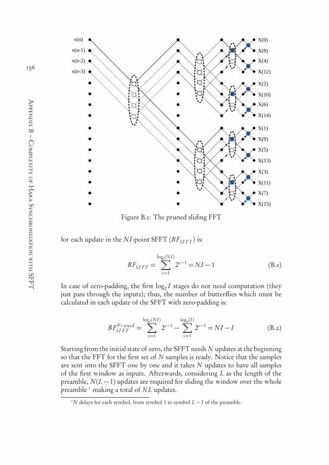
550999-L-bw-Siavash550999-L-bw-Siavash550999-L-bw-Siavash550999-L-bw-SiavashProcessed on: 23-11-2020Processed on: 23-11-2020Processed on: 23-11-2020Processed on: 23-11-2020 PDF page: 178PDF page: 178PDF page: 178PDF page: 178
156
AppendixB–ComplexityofHaraSynchronizationwithSFFT
x(n)
x(n-1)
x(n-2)
x(n-3)
X(0)
X(1)
X(15)
X(2)
X(3)
X(4)
X(5)
X(6)
X(7)
X(8)
X(9)
X(10)
X(11)
X(12)
X(13)
X(14)
Figure B.1: The pruned sliding FFT
for each update in the N I -point SFFT (BFSF F T ) is:
BFSF F T =log2(N I )∑
s=1
2s−1 =N I − 1 (B.1)
In case of zero-padding, the first log2 I stages do not need computation (theyjust pass through the inputs); thus, the number of butterflies which must becalculated in each update of the SFFT with zero-padding is:
BF P r unedSF F T =
log2(N I )∑
s=1
2s−1−log2(I )∑
s=1
2s−1 =N I − I (B.2)
Starting from the initial state of zero, the SFFT needs N updates at the beginningso that the FFT for the first set of N samples is ready. Notice that the samplesare sent into the SFFT one by one and it takes N updates to have all samplesof the first window as inputs. Afterwards, considering L as the length of thepreamble, N (L− 1) updates are required for sliding the window over the wholepreamble 1 making a total of N L updates.
1N delays for each symbol, from symbol 1 to symbol L− 1 of the preamble.

550999-L-bw-Siavash550999-L-bw-Siavash550999-L-bw-Siavash550999-L-bw-SiavashProcessed on: 23-11-2020Processed on: 23-11-2020Processed on: 23-11-2020Processed on: 23-11-2020 PDF page: 179PDF page: 179PDF page: 179PDF page: 179
157
AppendixB–ComplexityofHaraSynchronizationwithSFFT
Each butterfly is composed of one complex multiplication and two complex ad-ditions. So the number of complex multiplications and additions for calculatingthe SFFT are as follows.
C MSF F T =N L×BF P r unedSF F T (B.3)
C ASF F T = 2×N L×BF P r unedSF F T (B.4)
Now that the required number of operations are calculated for each part ofsynchronization, memory usage is calculated in the following.
In case of the SFFT, for the outputs of each butterfly (two outputs) in theFFT which is not calculated during an SFFT update, two memories are neededto store their values from the previous window [30]. As discussed earlier, forall first log2 I stages of the pruned SFFT only N − 1 previous input samplesmust be stored as these stages only pass through input samples. For the otherlog2 N stages, there are N I/2 butterflies per stage and (N I/2) log2 N butterfliesin total. Among these only I (N − 1) butterflies are calculated according toabove discussion and the rest use the stored value from the previous windowcalculations; thus, the required memory for calculation of SFFT is equal to:
M SF F TC al c = 2× [(N − 1)+ 2× ((N I/2) log2 N − I (N − 1))], (B.5)
where the first term in the right side of the equation is for storing the previoussamples and the second one is the required memory for butterfly outputs. Thefactor two before the brackets in (B.5) is the result of the fact that the valuesare complex and need two memories for storage. Besides, the factor two in thesecond term inside the bracket shows the number of outputs for each butterfly.
To compute the memory used for the accumulation of DFT bin values, M SF F TAcc ,
it should be noticed that for each delay value two sets of memories are used tostore the accumulated DFT bins magnitudes; odd and even symbols. For theconventional algorithm, each DFT has N I bins. So, considering N delay valueswe have:
M SF F TAcc = 2I N 2 (B.6)

550999-L-bw-Siavash550999-L-bw-Siavash550999-L-bw-Siavash550999-L-bw-SiavashProcessed on: 23-11-2020Processed on: 23-11-2020Processed on: 23-11-2020Processed on: 23-11-2020 PDF page: 180PDF page: 180PDF page: 180PDF page: 180
158
550999-L-bw-Siavash550999-L-bw-Siavash550999-L-bw-Siavash550999-L-bw-SiavashProcessed on: 23-11-2020Processed on: 23-11-2020Processed on: 23-11-2020Processed on: 23-11-2020 PDF page: 181PDF page: 181PDF page: 181PDF page: 181
159CHybrid Demodulator in
Time-Varying Channel
In this appendix the detailed expressions for F0 and F1 are derived. SubstitutingYk from (6.25) to (6.27) and (6.28) we have:
F0 =4∑
k=1
a2(k+1)|h|2Xk
+4∑
k=1
ak+3k−1∑
i=1
a i−1p
1− a2hη∗k−i Xk
+4∑
k=1
ak−1k+3∑
i=1
a i−1p
1− a2h∗ηk+4−i Xk
(C.1)
F1 =4∑
k=1
a2(k+1)|h|2Xk e− jωs e p kTs
+4∑
k=1
e− jωs e p kTs
ak+3k−1∑
i=1
a i−1p
1− a2hη∗k−i Xk
+ ak−1k+3∑
i=1
a i−1p
1− a2h∗ηk+4−i Xk
(C.2)
From (6.6) and considering ES/N = 1 for easier notations (this assumptiondoes not affect generality as this factor is present in both distortion and signalcomponents), we can write Xk = exp( j (∆ωn kTs +∆ϕn +θ)) where all phasecomponents in Xk other than information bearing phase, ∆ϕn , are absorbed inθ. Since this extra phase component is removed at the second stage and does notaffect our calculations here, we may ignore that to simplify notations. Now, incase ∆ωn = 0, Xk can be taken out of the summation in (C.1) to achieve:

550999-L-bw-Siavash550999-L-bw-Siavash550999-L-bw-Siavash550999-L-bw-SiavashProcessed on: 23-11-2020Processed on: 23-11-2020Processed on: 23-11-2020Processed on: 23-11-2020 PDF page: 182PDF page: 182PDF page: 182PDF page: 182
160
AppendixC–HybridDemodulatorinTime-VaryingChannel
F0 = e j∆ϕn
4∑
k=1
a2(k+1)|h|2
+e j∆ϕn
4∑
k=1
ak+3k−1∑
i=1
a i−1p
1− a2hη∗k−i
+e j∆ϕn
4∑
k=1
ak−1k+3∑
i=1
a i−1p
1− a2h∗ηk+4−i
(C.3)
For N = 4, since ωs e p = 2π/T , we have e− jωs e p kTs = (− j )k . Thus, F1 is derivedas follow.
F1 = e j∆ϕn
4∑
k=1
a2(k+1)|h|2(− j )k
+e j∆ϕn
4∑
k=1
(− j )k ak+3k−1∑
i=1
a i−1p
1− a2hη∗k−i
+ (− j )k ak−1k+3∑
i=1
a i−1p
1− a2h∗ηk+4−i
(C.4)
Both F0 and F1 have a signal component (first term in both) and other termsresulting from distortion which is caused by the random variable ηi .
ηi ∼CN (0,σ2h ) and h describes the channel state at the beginning of the (n−
1)t h symbol. The effect of h is the same for all samples during symbol detection.Moreover, only the magnitude of h affects the signal component (the first termin (6.25)) and the phase component is removed by the autocorrelation stage.As a result, although strictly speaking h ∼ CN (1,σ2
h ), we can treat it as adeterministic variable when calculating the effect of distortion during these threesymbols.
In the distortion terms of both F0 and F1, e j∆ϕn can be absorbed in the ran-dom variable and since its magnitude is one it does not change the variance.Moreover,
p1− a2h∗ηi = (p
(1− a2)hη∗i )∗ is denoted as a random variable
ζi ∼ CN (0, (1− a2)|h|2σ2h ) . Using these, after some mathematical manipu-
lation we have:

550999-L-bw-Siavash550999-L-bw-Siavash550999-L-bw-Siavash550999-L-bw-SiavashProcessed on: 23-11-2020Processed on: 23-11-2020Processed on: 23-11-2020Processed on: 23-11-2020 PDF page: 183PDF page: 183PDF page: 183PDF page: 183
161
AppendixC–HybridDemodulatorinTime-VaryingChannel
F0 = e j∆ϕn
4∑
k=1
a2(k+1)|h|2+4∑
m=1
a2−m4∑
k=1
a2kζm
+7∑
m=5
am−68−m∑
k=1
a2kζm
+3∑
m=1
a2−m4∑
k=m+1
a2kζ ∗m (C.5)
F+1 ≈4∑
m=1
a2−m4∑
k=1
(− j )k a2kζm
+7∑
m=5
am−68−m∑
k=1
(− j )k+1a2kζm
+3∑
m=1
a2−m4∑
k=m+1
(− j )k a2kζ ∗m (C.6)
In (C.6), the term with the signal component is almost zero due to (− j )k factor.It is not exactly zero (thus the sign ≈) but it is negligible compared to the signalcomponent in F0 and noise components in F1. For other values of N , the sameconclusion can be achieved. The same factor (− j )k is the reason for lower powerof noise in F1.
Each component including ζm is a circularly symmetric Gaussian variable. Thesum of circularly symmetric Gaussian variables is a circularly symmetric variableas well with a variance equal to the sum of the variances; however, this is notexactly true if ζm is added to its conjugate ζ ∗m . In (C.5) and (C.6), for m = 1,2,3,components with ζm are added to components which include ζ ∗m . As a result,the obtained random variable is not precisely a circularly symmetric variable i.e.the variance of its real and imaginary parts are slightly different; nevertheless,the variance of the resulting random variable is still the sum of the variancesof ζm and ζ ∗m . For simpler calculations, we approximate this sum of randomvariables with a circularly symmetric Gaussian random variable with the samevariance. Thus, merging the last three terms (including ζm and ζ ∗m ) of F0 andall terms of F1, F0 and F1 can be written in the form of:
F0 =p
PS e− j∆ϕn +Æ
PN ,0ηT0 (C.7)
F+1 Ů
PN ,+1ηT1 (C.8)
where:

550999-L-bw-Siavash550999-L-bw-Siavash550999-L-bw-Siavash550999-L-bw-SiavashProcessed on: 23-11-2020Processed on: 23-11-2020Processed on: 23-11-2020Processed on: 23-11-2020 PDF page: 184PDF page: 184PDF page: 184PDF page: 184
162
AppendixC–HybridDemodulatorinTime-VaryingChannel
PS = S |h|4 (C.9)PN ,0 = Υ0|h|
2σ2h (1− a2) (C.10)
PN ,+1 = Υ+1|h|2σ2
h (1− a2) (C.11)
The random variables ηT0 and ηT
1 areCN (0,1) and S , PN ,0 and PN ,+1 are achievedin terms of a as follows.
S =
4∑
k=1
a2(k+1)
2
(C.12)
Υ0 =4∑
m=1
|a2−m4∑
k=1
a2k |2+7∑
m=5
|am−68−m∑
k=1
a2k |2
+3∑
m=1
|a2−m4∑
k=m+1
a2k |2 (C.13)
Υ+1 =4∑
m=1
|a2−m4∑
k=1
(− j )k a2k |2
+7∑
m=5
|am−68−m∑
k=1
(− j )k+1a2k |2
+3∑
m=1
|(a2−m4∑
k=m+1
(− j )k a2k |2 (C.14)

550999-L-bw-Siavash550999-L-bw-Siavash550999-L-bw-Siavash550999-L-bw-SiavashProcessed on: 23-11-2020Processed on: 23-11-2020Processed on: 23-11-2020Processed on: 23-11-2020 PDF page: 185PDF page: 185PDF page: 185PDF page: 185
163

550999-L-bw-Siavash550999-L-bw-Siavash550999-L-bw-Siavash550999-L-bw-SiavashProcessed on: 23-11-2020Processed on: 23-11-2020Processed on: 23-11-2020Processed on: 23-11-2020 PDF page: 186PDF page: 186PDF page: 186PDF page: 186
164

550999-L-bw-Siavash550999-L-bw-Siavash550999-L-bw-Siavash550999-L-bw-SiavashProcessed on: 23-11-2020Processed on: 23-11-2020Processed on: 23-11-2020Processed on: 23-11-2020 PDF page: 187PDF page: 187PDF page: 187PDF page: 187
165DBER Curves for
Hybrid Demodulator
In this chapter the detailed BER curves for the scenarios in Chapter 6 are pre-sented and discussed.
D.1 BER Curves for Constant Symbol Rate Scenario
For the sake of clarity, different combinations are compared in two cases. In CaseI, all combinations which can obtain repetition orders (RO) of two and threein Table 6.3 are compared. Case II considers the combinations which achieverepetition orders of 4 and 5. The diagrams for Case I also include 2PSK and2FSK (shown by 2P and 2F, respectively). Besides, Case II diagrams also includethe BER curves for DD8PSK (shown by 8P) as a reference for comparison.
The BER performance of the system in a Rayleigh fading channel for threedifferent maximum Doppler shift values is demonstrated in Figure D.1-FigureD.3. The graphs on the top and the bottom show Case I and Case II, respectively.In each graph, similar line patterns (solid, dotted and dash-dotted) correspondto the same RO.
As expected, for a time-invariant channel in Figure D.1a and Figure D.1b, 2Pis the best as higher orders and hybrid combinations do not add the diversitybut only degrade performance. As can be seen, adding FSK to PSK modulationin Rayleigh channel does not lead to considerable improvement. This is inagreementwith the conclusions in [35]. In all modulations, themost determinantfactor for the BER performance is the order of MPSK modulation.
Figure D.2a and Figure D.2b show the BER curves in presence of a time-varyingchannel with a Jakes spectrum and a maximum Doppler shift of 2 Hz. ForRO > 2 (solid lines in Case I and all curves in Case II), using hybrid modula-tion can decrease the required E I n f
b /N0 for BER=0.1% by 5 to almost 11 dBcompared to MPSK with the same RO. For a certain RO, increasing the FSK

550999-L-bw-Siavash550999-L-bw-Siavash550999-L-bw-Siavash550999-L-bw-SiavashProcessed on: 23-11-2020Processed on: 23-11-2020Processed on: 23-11-2020Processed on: 23-11-2020 PDF page: 188PDF page: 188PDF page: 188PDF page: 188
166
AppendixD
–BERCurvesforHybridDemodulator
5 10 15 20 25 30 3510−4
10−3
10−2
10−1
100
EInfb
/N0[dB]
BER 2P
2F
4P
4F
2F2P
8PSK
2F4P
4F2P
(a)
5 10 15 20 25 30 3510−4
10−3
10−2
10−1
100
EInfb
/N0[dB]
BER
8PSK
16PSK
2F8P
4F4P
2F16P
4F8P
(b)
Figure D.1: BER curves for the system of Figure 6.4 and constant symbol ratescenario. The channel model is Rayleigh with Dmax = 0. (a) and (b) show CaseI and Case II, respectively. Each line pattern (solid and dashdotted) belongs tothe same repetition order.
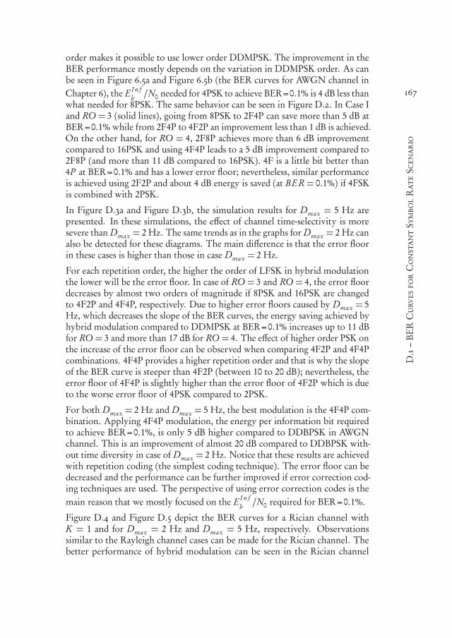
550999-L-bw-Siavash550999-L-bw-Siavash550999-L-bw-Siavash550999-L-bw-SiavashProcessed on: 23-11-2020Processed on: 23-11-2020Processed on: 23-11-2020Processed on: 23-11-2020 PDF page: 189PDF page: 189PDF page: 189PDF page: 189
167
D.1–BERCurvesforConstantSymbolRateScenario
order makes it possible to use lower order DDMPSK. The improvement in theBER performance mostly depends on the variation in DDMPSK order. As canbe seen in Figure 6.5a and Figure 6.5b (the BER curves for AWGN channel inChapter 6), the E I n f
b /N0 needed for 4PSK to achieve BER=0.1% is 4 dB less thanwhat needed for 8PSK. The same behavior can be seen in Figure D.2. In Case Iand RO = 3 (solid lines), going from 8PSK to 2F4P can save more than 5 dB atBER=0.1% while from 2F4P to 4F2P an improvement less than 1 dB is achieved.On the other hand, for RO = 4, 2F8P achieves more than 6 dB improvementcompared to 16PSK and using 4F4P leads to a 5 dB improvement compared to2F8P (and more than 11 dB compared to 16PSK). 4F is a little bit better than4P at BER=0.1% and has a lower error floor; nevertheless, similar performanceis achieved using 2F2P and about 4 dB energy is saved (at BER= 0.1%) if 4FSKis combined with 2PSK.
In Figure D.3a and Figure D.3b, the simulation results for Dmax = 5 Hz arepresented. In these simulations, the effect of channel time-selectivity is moresevere than Dmax = 2 Hz. The same trends as in the graphs for Dmax = 2 Hz canalso be detected for these diagrams. The main difference is that the error floorin these cases is higher than those in case Dmax = 2 Hz.
For each repetition order, the higher the order of LFSK in hybrid modulationthe lower will be the error floor. In case of RO = 3 and RO = 4, the error floordecreases by almost two orders of magnitude if 8PSK and 16PSK are changedto 4F2P and 4F4P, respectively. Due to higher error floors caused by Dmax = 5Hz, which decreases the slope of the BER curves, the energy saving achieved byhybrid modulation compared to DDMPSK at BER=0.1% increases up to 11 dBfor RO = 3 and more than 17 dB for RO = 4. The effect of higher order PSK onthe increase of the error floor can be observed when comparing 4F2P and 4F4Pcombinations. 4F4P provides a higher repetition order and that is why the slopeof the BER curve is steeper than 4F2P (between 10 to 20 dB); nevertheless, theerror floor of 4F4P is slightly higher than the error floor of 4F2P which is dueto the worse error floor of 4PSK compared to 2PSK.
For both Dmax = 2 Hz and Dmax = 5 Hz, the best modulation is the 4F4P com-bination. Applying 4F4P modulation, the energy per information bit requiredto achieve BER=0.1%, is only 5 dB higher compared to DDBPSK in AWGNchannel. This is an improvement of almost 20 dB compared to DDBPSK with-out time diversity in case of Dmax = 2 Hz. Notice that these results are achievedwith repetition coding (the simplest coding technique). The error floor can bedecreased and the performance can be further improved if error correction cod-ing techniques are used. The perspective of using error correction codes is themain reason that we mostly focused on the E I n f
b /N0 required for BER=0.1%.
Figure D.4 and Figure D.5 depict the BER curves for a Rician channel withK = 1 and for Dmax = 2 Hz and Dmax = 5 Hz, respectively. Observationssimilar to the Rayleigh channel cases can be made for the Rician channel. Thebetter performance of hybrid modulation can be seen in the Rician channel

550999-L-bw-Siavash550999-L-bw-Siavash550999-L-bw-Siavash550999-L-bw-SiavashProcessed on: 23-11-2020Processed on: 23-11-2020Processed on: 23-11-2020Processed on: 23-11-2020 PDF page: 190PDF page: 190PDF page: 190PDF page: 190
168
AppendixD
–BERCurvesforHybridDemodulator
5 10 15 20 25 30 3510−6
10−5
10−4
10−3
10−2
10−1
100
EInfb
/N0[dB]
BER 2P
2F
4P
4F
2F2P
8PSK
2F4P
4F2P
(a)
5 10 15 20 25 30 3510−6
10−5
10−4
10−3
10−2
10−1
100
EInfb
/N0[dB]
BER
8PSK
16PSK
2F8P
4F4P
2F16P
4F8P
(b)
Figure D.2: BER curves for the system of Figure 6.4 and constant symbol ratescenario. The channel model is Rayleigh with Dmax = 2 H z and Jakes Dopplerspectrum. (a) and (b) show Case I and Case II, respectively. Each line pattern(solid and dashdotted) belong to the same repetition order.

550999-L-bw-Siavash550999-L-bw-Siavash550999-L-bw-Siavash550999-L-bw-SiavashProcessed on: 23-11-2020Processed on: 23-11-2020Processed on: 23-11-2020Processed on: 23-11-2020 PDF page: 191PDF page: 191PDF page: 191PDF page: 191
169
D.1–BERCurvesforConstantSymbolRateScenario
5 10 15 20 25 30 3510−6
10−5
10−4
10−3
10−2
10−1
100
EInfb
/N0[dB]
BER 2P
2F
4P
4F
2F2P
8PSK
2F4P
4F2P
(a)
5 10 15 20 25 30 3510−6
10−5
10−4
10−3
10−2
10−1
100
EInfb
/N0[dB]
BER
8PSK
16PSK
2F8P
4F4P
2F16P
4F8P
(b)
Figure D.3: BER curves for the system of Figure 6.4 and constant symbol ratescenario. The channel model is Rayleigh with Dmax = 5 Hz and Jakes Dopplerspectrum. (a) and (b) show Case I and Case II, respectively. Each line pattern(solid and dashdotted) belongs to the same repetition order.

550999-L-bw-Siavash550999-L-bw-Siavash550999-L-bw-Siavash550999-L-bw-SiavashProcessed on: 23-11-2020Processed on: 23-11-2020Processed on: 23-11-2020Processed on: 23-11-2020 PDF page: 192PDF page: 192PDF page: 192PDF page: 192
170
AppendixD
–BERCurvesforHybridDemodulator
5 10 15 20 25 30 3510−6
10−5
10−4
10−3
10−2
10−1
100
EInfb
/N0[dB]
BER 2P
2F
4P
4F
2F2P
8PSK
2F4P
4F2P
(a)
5 10 15 20 25 30 3510−6
10−5
10−4
10−3
10−2
10−1
100
EInfb
/N0[dB]
BER
8PSK
16PSK
2F8P
4F4P
2F16P
4F8P
(b)
Figure D.4: BER curves for constant symbol rate scenario Case I (a) and CaseII (b). The channel model is Rician (K = 1) with Dmax = 2 Hz and a roundedDoppler spectrum.

550999-L-bw-Siavash550999-L-bw-Siavash550999-L-bw-Siavash550999-L-bw-SiavashProcessed on: 23-11-2020Processed on: 23-11-2020Processed on: 23-11-2020Processed on: 23-11-2020 PDF page: 193PDF page: 193PDF page: 193PDF page: 193
171
D.1–BERCurvesforConstantSymbolRateScenario
5 10 15 20 25 30 3510−6
10−5
10−4
10−3
10−2
10−1
100
EInfb
/N0[dB]
BER 2P
2F
4P
4F
2F2P
8P
2F4P
4F2P
(a)
5 10 15 20 25 30 3510−6
10−5
10−4
10−3
10−2
10−1
100
EInfb
/N0[dB]
BER
8PSK
16PSK
2F8P
4F4P
2F16P
4F8P
(b)
Figure D.5: BER curves for constant symbol rate scenario Case I (a) and CaseII (b). The channel model is Rician (K = 1) with Dmax = 5 Hz and a roundedDoppler spectrum.

550999-L-bw-Siavash550999-L-bw-Siavash550999-L-bw-Siavash550999-L-bw-SiavashProcessed on: 23-11-2020Processed on: 23-11-2020Processed on: 23-11-2020Processed on: 23-11-2020 PDF page: 194PDF page: 194PDF page: 194PDF page: 194
172
AppendixD
–BERCurvesforHybridDemodulator
as well. Similar to the Rayleigh channel results, the best combination is 4F4Pmodulation.
D.2 BER Curves for Equal Bandwidth Scenario
Two cases are investigated in this scenario. Case I and Case II which consider thetwo first columns of Table 6.4 and the last two columns of Table 6.4, respectively.All the combinations in each case have the same bandwidth (3RRe f
S for Case Iand 5RRe f
S for Case II) while providing various repetition orders.
The BER curves for the equal bandwidth scenario in a Rayleigh fading channelwith Dmax = 0 (constant channel) are shown in Figure D.6a and Figure D.6b.Since no diversity is added by increasing the raw bit-rate, a significant improve-ment is not expected for hybrid modulation. Similar to the constant symbolrate scenario, the performance of hybrid modulation schemes including 2PSKand 4PSK in a constant channel are very close while increasing the modulationorder to eight causes BER performance loss. The 2PSK (with increased symbolrate) has almost the same performance as the hybrid methods.
Figure D.7a and Figure D.7b demonstrate the BER curves for Dmax = 2 Hz andthe equal bandwidth scenario. For the lowest RO in both Case I and Case II(curves with triangle marker), hybrid modulation can save considerable energy(E I n f
b /N0 ) compared to DDMPSK; more than 10 dB in Case I and almost 5 dBin Case II at BER=0.1%. This significant difference is observed since the RO for2PSK with a higher symbol rate (1.5 and 2.5 when the symbol rate is 1.5RRe f
S
and 2.5RRe fS , respectively) is less than the ROs achieved by hybrid modulation
which are 2 and 3 for 2F2P and 4F2P, respectively (see Table 6.4). For 8PSK (thecurves with square markers), the hybrid modulation performs slightly betterthan faster 8PSK at BER=0.1% despite the fact that fast 8PSK achieves a higherrepetition order (RO) in both Case I and Case II. The difference between hybridmodulation and higher symbol rate 8PSK decreases when the E I n f
b increases(BER decreases). As can be seen the higher symbol rate MPSK crosses the hybridmodulation curve at BER=10−6 for Case I and BER< 10−6 for Case II.
The BER performance for Dmax = 5 Hz is shown in Figure D.8a and FigureD.8b. The same trends as explained for Dmax = 2 Hz are observed here aswell. The effect of increasing Dmax on the error floor of hybrid modulationis worse than its impact on higher symbol rate MPSK. As a consequence, theerror floor of hybrid modulation increases more than the error floor of fastDDMPSK which has a higher symbol rate. This brings the crossing point ofhybrid modulation and high symbol rate DDMPSK to higher than 10−6 whichwas the case in Dmax = 2 Hz. At a BER=0.1%, the 4F 4P requires the lowestE I n f
b /N0 values which is 2 dB less than the best DDMSPK (4PSK-2.5RS ).
The BER curves for a Rician channel with K = 1 and for Dmax = 2 Hz and

550999-L-bw-Siavash550999-L-bw-Siavash550999-L-bw-Siavash550999-L-bw-SiavashProcessed on: 23-11-2020Processed on: 23-11-2020Processed on: 23-11-2020Processed on: 23-11-2020 PDF page: 195PDF page: 195PDF page: 195PDF page: 195
173
D.2–BERCurvesforEqualBandwidthScenario
5 10 15 20 25 30 3510−4
10−3
10−2
10−1
100
EInfb
/N0[dB]
BER
2F2P
2PSK-1.5Rs
2F4P
4PSK-1.5Rs
2F8P
8PSK-1.5Rs
(a)
5 10 15 20 25 30 3510−3
10−2
10−1
100
EInfb
/N0[dB]
BER
4F2P
2PSK-2.5Rs
4F4P
4PSK-2.5Rs
4F8P
8PSK-2.5Rs
(b)
Figure D.6: BER curves for the system of Figure 6.4 and equal bandwidth sce-nario. The channel model is Rayleigh with Dmax = 0 and Jakes Doppler spec-trum. (a) and (b) show Case I and Case II, respectively. Each marker/colorcorresponds to one PSK order; triangle (black), circle (blue) and square (red)show 2PSK, 4PSK and 8PSK, respectively. For each color/marker, the solid linesshow the hybrid modulation and the dash-dotted lines show the correspondingMPSK modulation with increased symbol rate.

550999-L-bw-Siavash550999-L-bw-Siavash550999-L-bw-Siavash550999-L-bw-SiavashProcessed on: 23-11-2020Processed on: 23-11-2020Processed on: 23-11-2020Processed on: 23-11-2020 PDF page: 196PDF page: 196PDF page: 196PDF page: 196
174
AppendixD
–BERCurvesforHybridDemodulator
5 10 15 20 25 30 3510−6
10−5
10−4
10−3
10−2
10−1
100
EInfb
/N0[dB]
BER
2F2P
2PSK-1.5Rs
2F4P
4PSK-1.5Rs
2F8P
8PSK-1.5Rs
(a)
5 10 15 20 25 30 3510−6
10−5
10−4
10−3
10−2
10−1
100
EInfb
/N0[dB]
BER
4F2P
2PSK-2.5Rs
4F4P
4PSK-2.5Rs
4F8P
8PSK-2.5Rs
(b)
Figure D.7: BER curves for the system of Figure 6.4 and equal bandwidth sce-nario. The channel model is Rayleigh with Dmax = 2 Hz and Jakes Dopplerspectrum. (a) and (b) show Case I and Case II, respectively. Each marker/colorcorresponds to one PSK order; triangle (black), circle (blue) and square (red)show 2PSK, 4PSK and 8PSK, respectively. For each color/marker, the solid linesshow the hybrid modulation and the dash-dotted lines show the correspondingDDMPSK modulation with increased symbol rate.

550999-L-bw-Siavash550999-L-bw-Siavash550999-L-bw-Siavash550999-L-bw-SiavashProcessed on: 23-11-2020Processed on: 23-11-2020Processed on: 23-11-2020Processed on: 23-11-2020 PDF page: 197PDF page: 197PDF page: 197PDF page: 197
175
D.2–BERCurvesforEqualBandwidthScenario
5 10 15 20 25 30 3510−6
10−5
10−4
10−3
10−2
10−1
100
EInfb
/N0[dB]
BER
2F2P
2PSK-1.5Rs
2F4P
4PSK-1.5Rs
2F8P
8PSK-1.5Rs
(a)
5 10 15 20 25 30 3510−6
10−5
10−4
10−3
10−2
10−1
100
EInfb
/N0[dB]
BER
4F2P
2PSK-2.5Rs
4F4P
4PSK-2.5Rs
4F8P
8PSK-2.5Rs
(b)
Figure D.8: BER curves for the system of Figure 6.4 and equal bandwidth sce-nario. The channel model is Rayleigh with Dmax = 5 Hz and Jakes Dopplerspectrum. (a) and (b) show Case I and Case II, respectively. Each marker/colorcorresponds to one PSK order; triangle (black), circle (blue) and square (red)show 2PSK, 4PSK and 8PSK, respectively. For each color/marker, the solid linesshow the hybrid modulation and the dash-dotted lines show the correspondingMPSK modulation with increased symbol rate.

550999-L-bw-Siavash550999-L-bw-Siavash550999-L-bw-Siavash550999-L-bw-SiavashProcessed on: 23-11-2020Processed on: 23-11-2020Processed on: 23-11-2020Processed on: 23-11-2020 PDF page: 198PDF page: 198PDF page: 198PDF page: 198
176
AppendixD
–BERCurvesforHybridDemodulator
Dmax = 5 Hz are presented in Figure D.9 and Figure D.10, respectively. Similartrends as mentioned for a Rayleigh channel can be seen for a Rician channel.However, error floors for the hybrid modulation are much lower compared tothe Raleigh channel and the BER curve of a fast DDMPSK does not cross the hy-brid modulation curves in the range of BER> 10−6. In a Rician channel, the bestmodulation is 4F4P which is more than 2 dB better than the best combinationof 4PSK and higher symbol rate (4PSK-2.5RS ) at BER=0.1%.
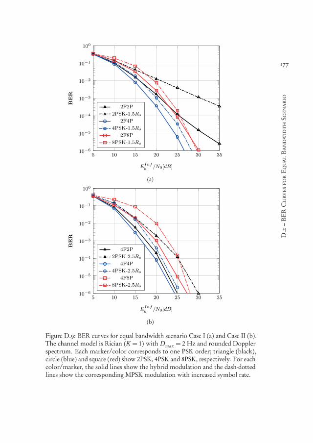
550999-L-bw-Siavash550999-L-bw-Siavash550999-L-bw-Siavash550999-L-bw-SiavashProcessed on: 23-11-2020Processed on: 23-11-2020Processed on: 23-11-2020Processed on: 23-11-2020 PDF page: 199PDF page: 199PDF page: 199PDF page: 199
177
D.2–BERCurvesforEqualBandwidthScenario
5 10 15 20 25 30 3510−6
10−5
10−4
10−3
10−2
10−1
100
EInfb
/N0[dB]
BER
2F2P
2PSK-1.5Rs
2F4P
4PSK-1.5Rs
2F8P
8PSK-1.5Rs
(a)
5 10 15 20 25 30 3510−6
10−5
10−4
10−3
10−2
10−1
100
EInfb
/N0[dB]
BER
4F2P
2PSK-2.5Rs
4F4P
4PSK-2.5Rs
4F8P
8PSK-2.5Rs
(b)
Figure D.9: BER curves for equal bandwidth scenario Case I (a) and Case II (b).The channel model is Rician (K = 1) with Dmax = 2 Hz and rounded Dopplerspectrum. Each marker/color corresponds to one PSK order; triangle (black),circle (blue) and square (red) show 2PSK, 4PSK and 8PSK, respectively. For eachcolor/marker, the solid lines show the hybrid modulation and the dash-dottedlines show the corresponding MPSK modulation with increased symbol rate.

550999-L-bw-Siavash550999-L-bw-Siavash550999-L-bw-Siavash550999-L-bw-SiavashProcessed on: 23-11-2020Processed on: 23-11-2020Processed on: 23-11-2020Processed on: 23-11-2020 PDF page: 200PDF page: 200PDF page: 200PDF page: 200
178
AppendixD
–BERCurvesforHybridDemodulator
5 10 15 20 25 30 3510−6
10−5
10−4
10−3
10−2
10−1
100
EInfb
/N0[dB]
BER
2F2P
2PSK-1.5Rs
2F4P
4PSK-1.5Rs
2F8P
8PSK-1.5Rs
(a)
5 10 15 20 25 30 3510−6
10−5
10−4
10−3
10−2
10−1
100
EInfb
/N0[dB]
BER
4F2P
2PSK-2.5Rs
4F4P
4PSK-2.5Rs
4F8P
8PSK-2.5Rs
(b)
Figure D.10: BER curves for equal bandwidth scenario Case I (a) and Case II (b).The channel model is Rician (K = 1) with Dmax = 5 Hz and rounded Dopplerspectrum. Each marker/color corresponds to one PSK order; triangle (black),circle (blue) and square (red) show 2PSK, 4PSK and 8PSK, respectively. For eachcolor/marker, the solid lines show the hybrid modulation and the dash-dottedlines show the corresponding MPSK modulation with increased symbol rate.

550999-L-bw-Siavash550999-L-bw-Siavash550999-L-bw-Siavash550999-L-bw-SiavashProcessed on: 23-11-2020Processed on: 23-11-2020Processed on: 23-11-2020Processed on: 23-11-2020 PDF page: 201PDF page: 201PDF page: 201PDF page: 201
179

550999-L-bw-Siavash550999-L-bw-Siavash550999-L-bw-Siavash550999-L-bw-SiavashProcessed on: 23-11-2020Processed on: 23-11-2020Processed on: 23-11-2020Processed on: 23-11-2020 PDF page: 202PDF page: 202PDF page: 202PDF page: 202
180

550999-L-bw-Siavash550999-L-bw-Siavash550999-L-bw-Siavash550999-L-bw-SiavashProcessed on: 23-11-2020Processed on: 23-11-2020Processed on: 23-11-2020Processed on: 23-11-2020 PDF page: 203PDF page: 203PDF page: 203PDF page: 203
181Acronyms
A ACD Auto-Correlation DemodulatorADC Analog to Digital ConverterAWGN Additive White Gaussian Noise
B BER Bit Error RateBFSK Binary FSKBoI Bins of Interest
C C-SDFT Complete SDFTCA Complex AdditionCDM Cross Differentiate MultiplyCFO Carrier Frequency OffsetCM Complex MultiplicationCPFSK Continuous Phase FSK
D DBFSK Differential Binary FSKDBPSK Binary DPSKDDBPSK Binary DDPSKDDMPSK Double Differential M-ary PSKDDPSK Double Differential PSKDFT Discrete Fourier TransformDLFSK Differential L-ary FSKDLL Delay Locked LoopDPSK Differential PSKDTFT Discrete Time Fourier Transform
F FFT Fast Fourier TransformFPSK Frequency/Phase Shift KeyingFSK Frequency Shift Keying
I IF Intermediate FrequencyIoT Internet of Things
L LEO Low Earth OrbitLFSK L-ary FSKLO Local OscillatorLPF Low-Pass FilterLPWAN Low Power Wide Area Network

550999-L-bw-Siavash550999-L-bw-Siavash550999-L-bw-Siavash550999-L-bw-SiavashProcessed on: 23-11-2020Processed on: 23-11-2020Processed on: 23-11-2020Processed on: 23-11-2020 PDF page: 204PDF page: 204PDF page: 204PDF page: 204
182
Acronyms
M MAC Medium Access ControlMAP Maximum a PosterioriMF Matched FilterMPSK M-ary PSK
N NB-IoT Narrowband IoT
O OFDM Orthogonal Frequency Division Multiplexing
P PSK Phase Shift Keying
Q Q2PSK Quadrature/Quadrature Phase Shift KeyingQFPM Quadrature Frequency/Phase ModulationQoS Quality of ServiceQPSK Quadrature PSK
R RO Repetition Order
S SB-SDFT Single Bin SDFTSDFT Sliding DFTSFFT Sliding FFTSNR Signal to Noise RatioST-DFT Short-Time Discrete Fourier Transform
U UNB Ultra-Narrowband
V VCO Voltage Controlled Oscillator
W WSN Wireless Sensor Networks
550999-L-bw-Siavash550999-L-bw-Siavash550999-L-bw-Siavash550999-L-bw-SiavashProcessed on: 23-11-2020Processed on: 23-11-2020Processed on: 23-11-2020Processed on: 23-11-2020 PDF page: 205PDF page: 205PDF page: 205PDF page: 205
183Bibliography
[1] LoRa. Available at https://lora-alliance.org/ (2020/08/18). (Cited onpage 3).
[2] Sigfox. Available at https://www.sigfox.com/en (2020/08/18). (Cited onpages 3, 4, and 128).
[3] Telensa. Available at https://www.telensa.com/ (2020/08/18). (Cited onpages 3 and 4).
[4] Weightless. Available at http://www.weightless.org/ (2020/08/18). (Cited onpages 3 and 4).
[5] L. Ahumada, R. Feick, and R. A. Valenzuela. Characterization of temporal fadingin urban fixed wireless links. IEEE Communications Letters, 10(4):242–244, April2006. (Cited on page 128).
[6] I. F. Akyildiz, W. Su, Y. Sankarasubramaniam, and E. Cayirci. Wireless sensornetworks: a survey. Computer networks, 38(4):393–422, 2002. (Cited on page 1).
[7] A. Al-Fuqaha, M. Guizani, M. Mohammadi, M. Aledhari, and M. Ayyash. In-ternet of things: A survey on enabling technologies, protocols, and applications.IEEE communications surveys & tutorials, 17(4):2347–2376, 2015. (Cited on page 1).
[8] G. Anastasi, M. Conti, M. Di Francesco, and A. Passarella. Energy conservationin wireless sensor networks: A survey. Ad hoc networks, 7(3):537–568, 2009. (Citedon page 1).
[9] M. Augustyniak and L. G. Doray. Inference for a leptokurtic symmetric familyof distributions represented by the difference of two gamma variates. Journal ofStatistical Computation and Simulation, 82(11):1621–1634, 2012. (Cited on page 65).
[10] K. E. Baddour and N. C. Beaulieu. Autoregressive modeling for fading channelsimulation. IEEE Transactions on Wireless Communications, 4(4):1650–1662, 2005.(Cited on page 116).
[11] L. M. Borges, F. J. Velez, and A. S. Lebres. Survey on the characterization and clas-sification of wireless sensor network applications. IEEE Communications Surveys& Tutorials, 16(4):1860–1890, 2014. (Cited on page 1).
[12] J. Buetefuer and W. G. Cowley. Frequency offset insensitive multiple symboldetection of MPSK. In 2000 IEEE International Conference on Acoustics, Speech,and Signal Processing. Proceedings (Cat. No. 00CH37100), volume 5, pages 2669–2672. IEEE, 2000. (Cited on pages 54 and 55).
550999-L-bw-Siavash550999-L-bw-Siavash550999-L-bw-Siavash550999-L-bw-SiavashProcessed on: 23-11-2020Processed on: 23-11-2020Processed on: 23-11-2020Processed on: 23-11-2020 PDF page: 206PDF page: 206PDF page: 206PDF page: 206
184
Bibliography
[13] B. Buurman, J. Kamruzzaman, G. Karmakar, and S. Islam. Low-Power Wide-Area Networks: Design goals, architecture, suitability to use cases and researchchallenges. IEEE Access, 8:17179–17220, 2020. (Cited on page 2).
[14] S. Byun, C.-H. Park, Y. Song, S. Wang, C. S. Conroy, and B. Kim. A low-powerCMOS bluetooth RF transceiver with a digital offset canceling DLL-based GFSKdemodulator. IEEE Journal of Solid-State Circuits, 38(10):1609–1618, 2003. (Citedon pages 6 and 18).
[15] K. V. Cartwright and E. J. Kaminsky. An optimum hardware detector for con-stant envelope quadrature-quadrature phase-shift keying (CEQ/sup 2/PSK). InGLOBECOM ’05. IEEE Global Telecommunications Conference, 2005., volume 1,pages 4 pp.–, Nov 2005. (Cited on page 21).
[16] C. Char-Dir. Differential detection of quadrature frequency/phase modulatedsignals. IEEE Transactions on Communications, 47(4):546–557, 1999. (Cited onpages 21 and 115).
[17] Char-Dir Chung and Fu-Chuan Hung. Noncoherent maximum-likelihood blockdetection of orthogonal NFSK-LDPSK signals. IEEE Transactions on VehicularTechnology, 51(2):283–292, March 2002. (Cited on pages 7 and 106).
[18] P. Chen, B. Zhao, R. Luo, and H. Yang. A low-power all-digital GFSK demodula-tor with robust clock data recovery. In Proceedings of the great lakes symposium onVLSI, pages 123–128, 2012. (Cited on page 6).
[19] Y.-C. Chen, Y.-C. Wu, and P.-C. Huang. A 1.2-v cmos limiter/rssi/demodulatorfor low-if fsk receiver. In 2007 IEEE Custom Integrated Circuits Conference, pages217–220. IEEE, 2007. (Cited on pages 6, 18, and 29).
[20] M. Covell and J. Richardson. A new, efficient structure for the short-time Fouriertransform, with an application in code-division sonar imaging. In [Proceedings]ICASSP 91: 1991 International Conference on Acoustics, Speech, and Signal Process-ing, pages 2041–2044 vol.3. (Cited on pages 76 and 80).
[21] D. Divsalar and M. K. Simon. Multiple-symbol differential detection of MPSK.IEEE Transactions on Communications, 38(3):300–308, Mar 1990. (Cited onpage 19).
[22] M.-T. Do, C. Goursaud, and J.-M. Gorce. On the benefits of random FDMAschemes in ultra narrow band networks. In 2014 12th International Symposiumon Modeling and Optimization in Mobile, Ad Hoc, and Wireless Networks (WiOpt),pages 672–677. IEEE, 2014. (Cited on page 3).
[23] I. Domuta and T. P. Palade. Sliding DFT and zero padding. In 2019 42nd Interna-tional Conference on Telecommunications and Signal Processing (TSP), pages 154–157.IEEE, 2019. (Cited on page 83).
[24] S. C. Douglas and J. K. Soh. A numerically-stable sliding-window estimator andits application to adaptive filters. In Conference Record of the Thirty-First AsilomarConference on Signals, Systems and Computers (Cat. No.97CB36136), volume 1, pages111–115 vol.1. (Cited on pages 76 and 80).
550999-L-bw-Siavash550999-L-bw-Siavash550999-L-bw-Siavash550999-L-bw-SiavashProcessed on: 23-11-2020Processed on: 23-11-2020Processed on: 23-11-2020Processed on: 23-11-2020 PDF page: 207PDF page: 207PDF page: 207PDF page: 207
185
Bibliography
[25] D. Duchemin, J.-M. Gorce, and C. Goursaud. Low complexity detector formassive uplink random access with NOMA in IoT LPWA networks. In 2019
IEEE Wireless Communications and Networking Conference Workshop (WCNCW),pages 1–6. IEEE, 2019. (Cited on page 3).
[26] K. Duda. Accurate, guaranteed stable, sliding Discrete Fourier Transform. IEEESignal Processing Magazine, 27(6):124–127, 2010. ISSN 1053-5888. (Cited onpages 76, 80, 83, 89, and 90).
[27] O. M. El-Ghandour and D. Saha. Differential detection in quadrature-quadraturephase shift keying (Q/sup 2/PSK) systems. IEEE Transactions onCommunications,39(5):703–712, May 1991. (Cited on page 21).
[28] V. Erceg et al. Channel Models for Fixed Wireless Applications. IEEE 802.16 Broad-band Wireless Access Working Group, 2001. (Cited on page 129).
[29] A. G. Exposito and J. A. R. Macfas. Fast non-recursive computation of individualrunning harmonics. IEEE Transactions on Circuits and Systems II: Analog andDigital Signal Processing, 47(8):779–782, 2000. (Cited on pages 76 and 80).
[30] B. Farhang-Boroujeny and S. Gazor. Generalized sliding FFT and its applicationto implementation of block LMS adaptive filters. IEEE Transactions on SignalProcessing, 42(3):532–538, March 1994. (Cited on pages 80, 81, 82, 94, 155, and 157).
[31] B. Farhang-Boroujeny and Y. C. Lim. A comment on the computational com-plexity of sliding FFT. IEEE Transactions on Circuits and Systems II: Analog andDigital Signal Processing, 39(12):875–876, 1992. (Cited on pages 76 and 80).
[32] M. J. Farooq and Q. Zhu. Optimal dynamic contract for spectrum reservationin mission-critical UNB-IoT systems. In 2018 16th International Symposium onModeling and Optimization in Mobile, Ad Hoc, and Wireless Networks (WiOpt),pages 1–6. IEEE, 2018. (Cited on page 3).
[33] S. Fleisher and Shouxing Qu. Quadrature frequency/phase modulation. IEEETransactions on Communications, 43(2/3/4):1513–1524, Feb 1995. (Cited onpage 21).
[34] I. Ghareeb. Bit error rate performance and power spectral density of a noncoherenthybrid frequency-phase modulation system. IEEE Journal on Selected Areas inCommunications, 13(2):276–284, 1995. (Cited on pages 7, 22, 106, 107, 109, 115,and 125).
[35] I. Ghareeb and A. Yongacoglu. Performance of joint frequency phase modulationover Rayleigh fading channels. IEE Proceedings - Communications, 141(4):241–247,1994. (Cited on pages 7, 106, 107, 115, and 165).
[36] K. S. Gomadam and S. A. Jafar. Modulation and detection for simple receiversin rapidly time-varying channels. IEEE Transactions on Communications, 55(3):529–539, 2007. (Cited on pages 115 and 116).
[37] C. Goursaud and J. Gorce. Dedicated networks for IoT: PHY/MAC state ofthe art and challenges. EAI Endorsed Transactions on Internet of Things, 1(1), 2015.(Cited on page 6).

550999-L-bw-Siavash550999-L-bw-Siavash550999-L-bw-Siavash550999-L-bw-SiavashProcessed on: 23-11-2020Processed on: 23-11-2020Processed on: 23-11-2020Processed on: 23-11-2020 PDF page: 208PDF page: 208PDF page: 208PDF page: 208
186
Bibliography
[38] C. Goursaud and Y. Mo. Random unslotted time-frequency ALOHA: Theoryand application to IoT UNB networks. In 2016 23rd International Conferenceon Telecommunications (ICT), pages 1–5. IEEE, 2016. (Cited on pages 3, 5, 6, 7,and 106).
[39] E. Grayver and B. Daneshrad. A low-power all-digital FSK receiver for spaceapplications. IEEE Transactions on Communications, 49(5):911–921, 2001. (Citedon pages 7, 27, and 30).
[40] L. J. Greenstein, S. S. Ghassemzadeh, V. Erceg, and D. G. Michelson. Riceank-factors in narrow-band fixed wireless channels: Theory, experiments, and sta-tistical models. IEEE Transactions on Vehicular Technology, 58(8):4000–4012, Oct2009. (Cited on page 128).
[41] F. Gu, J. Niu, L. Jiang, X. Liu, and M. Atiquzzaman. Survey of the low powerwide area network technologies. Journal of Network and Computer Applications,149:102459, 2020. (Cited on page 2).
[42] D. A. Gudovskiy and L. Chu. An accurate and stable sliding DFT computed bya modified CIC filter. IEEE Signal Processing Magazine, 34(1):89–93, 2017. (Citedon pages 76 and 80).
[43] D. Han and Y. Zheng. A mixed-signal GFSK demodulator based on multithresh-old linear phase quantization. IEEE Transactions on Circuits and Systems II: ExpressBriefs, 56(9):719–723, 2009. (Cited on pages 6, 17, and 29).
[44] S. Hara, A. Wannasarnmaytha, Y. Tsuchida, and N. Morinaga. A novel FSKdemodulation method using short-time DFT analysis for LEO satellite commu-nication systems. IEEE Transactions on Vehicular Technology, 46(3):625–633, Aug1997. (Cited on pages 7, 27, 28, 30, 31, 32, 33, 35, 47, 77, and 112).
[45] S. Haykin. Digital Communication Systems. Wiley, 2013. ISBN 9780471647355.(Cited on pages 14, 15, 16, 38, 44, 45, 118, and 119).
[46] K. Henning. Recommendations for implementing the strategic initiative industrie4.0. 2013. (Cited on page 1).
[47] N. Instruments. Introduction to Bluetooth device testing: From theory to trans-mitter and receiver measurements. Technical report, National Instruments, 2016.(Cited on pages 5 and 28).
[48] E. Jacobsen and R. Lyons. The sliding DFT. IEEE Signal Processing Magazine, 20(2):74–80, March 2003. (Cited on pages 76, 80, 82, 83, 89, and 90).
[49] D. W. Jang and T. H. Choi. Decision feedback-based demodulation of doublydifferential PSK signals. IEEE Transactions on Communications, 48(8):1253–1256,Aug 2000. (Cited on pages 6 and 54).
[50] H.-S. Kao, M.-J. Yang, and T.-C. Lee. A delay-line-based GFSK demodulator forlow-IF receivers. In 2007 IEEE International Solid-State Circuits Conference. Digestof Technical Papers, pages 88–589. IEEE, 2007. (Cited on pages 6, 18, and 29).
550999-L-bw-Siavash550999-L-bw-Siavash550999-L-bw-Siavash550999-L-bw-SiavashProcessed on: 23-11-2020Processed on: 23-11-2020Processed on: 23-11-2020Processed on: 23-11-2020 PDF page: 209PDF page: 209PDF page: 209PDF page: 209
187
Bibliography
[51] P. Karadimas, E. D. Vagenas, and S. A. Kotsopoulos. On the scatterers’ mobilityand second order statistics of narrowband fixed outdoor wireless channels. IEEETransactions on Wireless Communications, 9(7):2119–2124, July 2010. (Cited onpage 128).
[52] R. A. Khalona, G. E. Atkin, and J. L. LoCicero. On the performance of a hybridfrequency and phase shift keying modulation technique. IEEE Transactions onCommunications, 41(5):655–659, 1993. (Cited on pages 7, 106, 107, and 125).
[53] Z. Kollar, F. Plesznik, and S. Trumpf. Observer-based recursive sliding DiscreteFourier Transform. IEEE Signal Processing Magazine, 35(6):100–106, 2018. (Citedon pages 76, 80, and 82).
[54] K. Krishnamoorthy. Handbook of statistical distributions with applications. CRCPress, 2016. (Cited on page 64).
[55] D. Lachartre, F. Dehmas, C. Bernier, C. Fourtet, L. Ouvry, F. Lepin, E. Mercier,S. Hamard, L. Zirphile, S. Thuries, and F. Chaix. 7.5 a TCXO-less 100 Hz-minimum-bandwidth transceiver for ultra-narrow-band sub-GHz IoT cellular net-works. In 2017 IEEE International Solid-State Circuits Conference (ISSCC), pages134–135, Feb 2017. (Cited on pages 5, 6, 8, 106, and 128).
[56] T.-C. Lee and C.-C. Chen. A mixed-signal GFSK demodulator for Bluetooth.IEEE Transactions on Circuits and Systems II: Express Briefs, 53(3):197–201, 2006.(Cited on pages 6, 16, and 29).
[57] W. Lei and I. Korn. Combined frequency and differential phase shift keyingwith non-coherent detection in a satellite mobile channel. IEEE Transactions onVehicular Technology, 44(3):603–612, 1995. (Cited on pages 7, 106, 115, and 125).
[58] H. Leib. Data-aided noncoherent demodulation of DPSK. IEEE transactions oncommunications, 43(2/3/4):722–725, 1995. (Cited on page 20).
[59] W. Lindsey and M. Simón. Telecommunication systems engineering. Prentice-Hallinformation and system sciences series. Prentice-Hall, 1973. ISBN 9780139024290.(Cited on page 107).
[60] J. Liu, S. Kwatra, and J. Kim. An analysis of decision feedback detection ofdifferentially encoded MPSK signals. IEEE transactions on vehicular technology, 44(2):261–267, 1995. (Cited on page 20).
[61] E. Lopelli, J. Van der Tang, and A. H. van Roermund. A FSK demodulatorcomparison for ultra-low power, low data-rate wireless links in ISM bands. InProceedings of the 2005 European Conference on Circuit Theory and Design, 2005.,volume 2, pages II–259. IEEE, 2005. (Cited on pages 29 and 30).
[62] R. W. Ltd. A comparison of UNB and spread spectrum wireless technologies asused in LPWA M2M applications. Technical report, Real Wireless, West Succex,UK, 2015. (Cited on pages 2, 3, and 4).

550999-L-bw-Siavash550999-L-bw-Siavash550999-L-bw-Siavash550999-L-bw-SiavashProcessed on: 23-11-2020Processed on: 23-11-2020Processed on: 23-11-2020Processed on: 23-11-2020 PDF page: 210PDF page: 210PDF page: 210PDF page: 210
188
Bibliography
[63] M. Z. Mahfouz, A. Meijerink, and M. J. Bentum. Ultra-narrowband for energy-scavenging-powered wireless sensor networks. In 2017 IEEE 28th Annual Interna-tional Symposium on Personal, Indoor, and Mobile Radio Communications (PIMRC),pages 1–7. IEEE, 2017. (Cited on page 4).
[64] P. Mak, S. U, and R. P. Martins. Transceiver architecture selection: Review, state-of-the-art survey and case study. IEEE Circuits and Systems Magazine, 7(2):6–25,2007. (Cited on page 8).
[65] G. Meciani. Implementation of a power-efficient DFT based demodulator forBFSK (MSc. thesis), December 2018. (Cited on page 155).
[66] K. Mekki, E. Bajic, F. Chaxel, and F. Meyer. A comparative study of LPWANtechnologies for large-scale IoT deployment. ICT express, 5(1):1–7, 2019. (Citedon pages 3 and 4).
[67] U. Mengali. Synchronization Techniques for Digital Receivers. Applications ofCommunications Theory. Springer US, 2013. ISBN 9781489918079. (Cited onpage 23).
[68] H. Meyr, M. Moeneclaey, and S. Fechtel. Digital Communication Receivers, Vol-ume 2: Synchronization, Channel Estimation, and Signal Processing. Wiley Seriesin Telecommunications and Signal Processing. Wiley, 1997. ISBN 9780471502753.(Cited on pages 6, 23, and 24).
[69] Y. Mo, C. Goursaud, and J.-M. Gorce. Theoretical analysis of UNB-based IoTnetworks with path loss and random spectrum access. In 2016 IEEE 27th AnnualInternational Symposium on Personal, Indoor, and Mobile Radio Communications(PIMRC), pages 1–6. IEEE, 2016. (Cited on page 3).
[70] Y. Mo, C. Goursaud, and J.-M. Gorce. On the benefits of successive interferencecancellation for ultra narrow band networks: Theory and application to IoT. In2017 IEEE International Conference on Communications (ICC), pages 1–6. IEEE,2017. (Cited on page 3).
[71] A. Molisch. Wireless Communications. Wiley, 2012. ISBN 9781118355688. (Citedon pages 7, 105, 106, 115, and 130).
[72] D.-E. A. Montoya, J. A. Rosendo Macías, and A. Gómez-Expósito. Short-timeDFT computation by a modified radix-4 decimation-in-frequency algorithm. Sig-nal Processing, 94:81–89, 2014. (Cited on pages 76, 80, and 81).
[73] D. A.Montoya-Andrade, J. A. Rosendo-Macías, andA.Gómez-Expósito. Efficientcomputation of the short-time DFT based on a modified radix-2 decimation-in-frequency algorithm. Signal Processing, 92(10):2525–2531, 2012. (Cited on pages 76,80, and 81).
[74] N. Naik. LPWAN technologies for IoT systems: choice between ultra narrowband and spread spectrum. In 2018 IEEE International Systems Engineering Sym-posium (ISSE), pages 1–8. IEEE, 2018. (Cited on pages 3 and 4).

550999-L-bw-Siavash550999-L-bw-Siavash550999-L-bw-Siavash550999-L-bw-SiavashProcessed on: 23-11-2020Processed on: 23-11-2020Processed on: 23-11-2020Processed on: 23-11-2020 PDF page: 211PDF page: 211PDF page: 211PDF page: 211
189
Bibliography
[75] R. Ni, K. Mayaram, and T. S. Fiez. A 2.4GHz hybrid polyphase filter based BFSKreceiver with high frequency offset tolerance for wireless sensor networks. IEEEjournal of solid-state circuits, 48(5):1250–1263, 2013. (Cited on pages 6 and 29).
[76] K. E. Nolan, W. Guibene, and M. Y. Kelly. An evaluation of low power wide areanetwork technologies for the Internet of Things. In 2016 international wirelesscommunications and mobile computing conference (IWCMC), pages 439–444. IEEE,2016. (Cited on page 2).
[77] C. Oestges, D. Vanhoenacker-Janvier, and B. Clerckx. Channel characterizationof indoor wireless personal area networks. IEEE Transactions on Antennas andPropagation, 54(11):3143–3150, Nov 2006. (Cited on pages 128 and 129).
[78] C. Park. Fast, accurate, and guaranteed stable sliding Discrete Fourier Transform.IEEE Signal Processing Magazine, 32(4):145–156, July 2015. (Cited on pages 76, 80,81, and 89).
[79] C. Park. Guaranteed-stable sliding DFT algorithm with minimal computationalrequirements. IEEE Transactions on Signal Processing, 65(20):5281–5288, Oct 2017.(Cited on page 83).
[80] C.-S. Park and S.-J. Ko. The hopping Discrete Fourier Transform. IEEE SignalProcessing Magazine, 31(2):135–139, 2014. (Cited on pages 76, 80, and 81).
[81] M. H. Perrott, J. C. Salvia, F. S. Lee, A. Partridge, S. Mukherjee, C. Arft, J. Kim,N. Arumugam, P. Gupta, S. Tabatabaei, et al. A temperature-to-digital converterfor a MEMS-based programmable oscillator with ±5 ppm frequency stability and1 ps integrated jitter. IEEE Journal of Solid-State Circuits, 48(1):276–291, 2012.(Cited on page 5).
[82] J. Proakis and D. Manolakis. Digital Signal Processing. Pearson Prentice Hall,2007. ISBN 9780131873742. (Cited on page 147).
[83] Q. M. Qadir, T. A. Rashid, N. K. Al-Salihi, B. Ismael, A. A. Kist, and Z. Zhang.Low power wide area networks: a survey of enabling technologies, applicationsand interoperability needs. IEEE Access, 6:77454–77473, 2018. (Cited on pages 2and 4).
[84] A. M. Rabiei and N. C. Beaulieu. Frequency offset invariant multiple symboldifferential detection of MPSK. IEEE Transactions on Communications, 59(3):652–657, March 2011. (Cited on pages 6, 23, and 54).
[85] Z. Rafii. Sliding Discrete Fourier Transform with kernel windowing [lecturenotes]. IEEE Signal Processing Magazine, 35(6):88–92, 2018. (Cited on pages 76and 80).
[86] U. Raza, P. Kulkarni, andM. Sooriyabandara. Low power wide area networks: Anoverview. IEEE Communications Surveys & Tutorials, 19(2):855–873, 2017. (Citedon pages 2, 3, and 4).
[87] I. Reed and R. Scholtz. N-orthogonal phase-modulated codes. IEEE Transac-tions on Information Theory, 12(3):388–395, July 1966. (Cited on pages 7, 22, 106,and 107).

550999-L-bw-Siavash550999-L-bw-Siavash550999-L-bw-Siavash550999-L-bw-SiavashProcessed on: 23-11-2020Processed on: 23-11-2020Processed on: 23-11-2020Processed on: 23-11-2020 PDF page: 212PDF page: 212PDF page: 212PDF page: 212
190
Bibliography
[88] B. Reynders, W.Meert, and S. Pollin. Range and coexistence analysis of long rangeunlicensed communication. In 2016 23rd International Conference on Telecommu-nications (ICT), pages 1–6. IEEE, 2016. (Cited on page 3).
[89] S. Safapourhajari and A. B. J. Kokkeler. Frequency offset tolerant demodulationfor low data rate and narrowband wireless sensor node. In 2017 11th InternationalConference on Signal Processing and Communication Systems (ICSPCS), pages 1–8,Dec 2017. (Cited on pages 35, 77, and 97).
[90] D. Saha and T. G. Birdsall. Quadrature-quadrature phase-shift keying. IEEETransactions on Communications, 37(5):437–448, May 1989. (Cited on pages 20and 21).
[91] R. Sanchez-Iborra and M.-D. Cano. State of the art in LP-WAN solutions forindustrial IoT services. Sensors, 16(5):708, 2016. (Cited on page 2).
[92] H.-Y. Shih, C.-F. Chen, Y.-C. Chang, and Y.-W. Hu. An ultralow power multirateFSK demodulator with digital-assisted calibrated delay-line based phase shifter forhigh-speed biomedical zero-IF receivers. IEEE Transactions on Very Large ScaleIntegration (VLSI) Systems, 23(1):98–106, 2014. (Cited on page 18).
[93] M. Simon, S. Hinedi, and W. Lindsey. Digital Communication Techniques: SignalDesign and Detection. Digital Communication Techniques. PTR Prentice Hall,1995. ISBN 9780132006101. (Cited on pages 38, 44, 53, 55, and 107).
[94] M. K. Simon and D. Divsalar. On the implementation and performance of singleand double differential detection schemes. IEEE Transactions on Communications,40(2):278–291, Feb 1992. ISSN 0090-6778. (Cited on pages 6, 7, 28, 36, 37, 38, 44,53, 54, 55, 56, 68, 111, 113, and 125).
[95] R. S. Sinha, Y. Wei, and S.-H. Hwang. A survey on LPWA technology: LoRa andNB-IoT. Ict Express, 3(1):14–21, 2017. (Cited on page 2).
[96] T. Šolc, T. Gale, and C. Fortuna. Optimization of ultra-narrowband wireless com-munication: An experimental case study. In 2017 IEEE Conference on ComputerCommunications Workshops (INFOCOM WKSHPS), pages 523–528. IEEE, 2017.(Cited on page 3).
[97] S. Stein. Fading channel issues in system engineering. IEEE Journal on SelectedAreas in Communications, 5(2):68–89, 1987. (Cited on page 120).
[98] P. Stoica, J. Liu, and J. Li. Maximum-likelihood double differential detectionclarified. IEEE Transactions on Information Theory, 50(3):572–576, 2004. (Citedon page 54).
[99] P. Stoica, J. Liu, J. Li, and M. A. Prasad. The heuristic, GLRT, andMAP detectorsfor double differential modulation are identical. IEEE Transactions on InformationTheory, 51(5):1860–1865, May 2005. ISSN 0018-9448. (Cited on pages 6 and 54).
[100] J.Wang, B.Woods, andW. F. Eddy. MEG,RFFTs, and the hunt for high frequencyoscillations. In 2009 2nd International Congress on Image and Signal Processing,pages 1–5. (Cited on pages 76, 80, and 81).
550999-L-bw-Siavash550999-L-bw-Siavash550999-L-bw-Siavash550999-L-bw-SiavashProcessed on: 23-11-2020Processed on: 23-11-2020Processed on: 23-11-2020Processed on: 23-11-2020 PDF page: 213PDF page: 213PDF page: 213PDF page: 213
191
Bibliography
[101] J.-M.Wang andW. F. Eddy. Parallel algorithm for SWFFT using 3D data structure.Circuits, Systems, and Signal Processing, 31(2):711–726, 2011. (Cited on pages 76, 80,and 81).
[102] B. Xia, C. Xin, W. Sheng, A. Y. Valero-Lopez, and E. Sánchez-Sinencio. A GFSKdemodulator for low-IF Bluetooth receiver. IEEE Journal of solid-state circuits, 38(8):1397–1400, 2003. (Cited on pages 6, 17, and 29).
[103] F. Xiong. Digital Modulation Techniques. Artech House telecommunicationslibrary. Artech House, 2000. ISBN 9780890069707. (Cited on pages 15, 43, 101,and 115).
[104] J. Yick, B. Mukherjee, and D. Ghosal. Wireless sensor network survey. Computernetworks, 52(12):2292–2330, 2008. (Cited on page 1).
[105] Y. Yin, Y. Yan, C. Wei, and S. Yang. A low-power low-cost GFSK demodulatorwith a robust frequency offset tolerance. IEEE Transactions on Circuits and SystemsII: Express Briefs, 61(9):696–700, 2014. (Cited on page 17).
[106] M. R. Yuce and W. Liu. A low-power multirate differential PSK receiver for spaceapplications. IEEE Transactions on Vehicular Technology, 54(6):2074–2084, Nov2005. (Cited on pages 6, 7, and 27).
[107] M. Yuqi, C. Goursaud, and J.-M. Gorce. Uplink multiple base stations diversityfor UNB based IoT networks. In 2018 IEEE Conference on Antenna Measurements& Applications (CAMA), pages 1–4. IEEE, 2018. (Cited on page 3).

550999-L-bw-Siavash550999-L-bw-Siavash550999-L-bw-Siavash550999-L-bw-SiavashProcessed on: 23-11-2020Processed on: 23-11-2020Processed on: 23-11-2020Processed on: 23-11-2020 PDF page: 214PDF page: 214PDF page: 214PDF page: 214
192
550999-L-bw-Siavash550999-L-bw-Siavash550999-L-bw-Siavash550999-L-bw-SiavashProcessed on: 23-11-2020Processed on: 23-11-2020Processed on: 23-11-2020Processed on: 23-11-2020 PDF page: 215PDF page: 215PDF page: 215PDF page: 215
193List of Publications
[S:1] S. Safapourhajari and A. B. J. Kokkeler. Offset tolerant hybrid demodulator andtime-diversity for ultra-narrowband communications. Manuscript submitted forpublication, 2020.
[S:2] Siavash Safapourhajari and André BJ Kokkeler. On the low complexity imple-mentation of the DFT-based BFSK demodulator for ultra-narrowband communi-cations. IEEE Access, 8:146666–146682, 2020.
[S:3] S. Safapourhajari and A. B. J. Kokkeler. Frequency offset tolerant demodulationfor low data rate and narrowband wireless sensor node. In 2017 11th InternationalConference on Signal Processing and Communication Systems (ICSPCS), pages 1–8,2017.
[S:4] S. Safapourhajari and A. B. J. Kokkeler. Demodulation of double differential PSKin presence of large frequency offset and wide filter. In 2018 IEEE 87th VehicularTechnology Conference (VTC Spring), pages 1–5, 2018.
[S:5] S. Safapourhajari and A. B. J. Kokkeler. Offset tolerant demodulator for frequen-cy/phase modulation in time-varying channel. In 2019 IEEE Wireless Communi-cations and Networking Conference (WCNC), pages 1–6, 2019.
[S:6] S. Safapourhajari and A. B. J. Kokkeler. Low complexity synchronization foroffset tolerant DFT-based BFSK demodulator. In 2019 IEEE 20th InternationalWorkshop on Signal Processing Advances in Wireless Communications (SPAWC),pages 1–5, 2019.
This thesis
@phdthesissafapour2020:thesis,author=Safapourhajari, Siavash,title=Frequency Offset Tolerant Demodulators for UNB Communications,school=University of Twente,address=PO Box 217, 7500 AE Enschede, The Netherlands,year=2020,month=dec,number=IDS Ph.D. Thesis Series No. 20-006,issn=2589-7721,isbn=978-90-365-5086-4,doi=10.3990/1.9789036550864
BibTEX of this thesis

Propositions
accompanying the thesis
Frequency Offset Tolerant Demodulatorsfor UNB Communications
by Siavash Safapourhajari,to be defended on vrijdag 11 december 2020
1 — Instead of using costly precise oscillators, demodulation algorithms can bedesigned such that they tolerate frequency inaccuracy. (This thesis)
2 — A concept or technique should not be dismissed just because it is not a hottopic anymore. Sometimes adapting old techniques to a new context can bringus interesting solutions. (This thesis)
3 — In most cases, an algorithm is designed and after that an efficient implementa-tion is devised. Sometimes, it is worth looking at this the other way around;see what efficient implementations exist and modify the algorithm to exploitthose implementations.
4 — In academic conferences, poster sessions are more efficient than parallel oralpresentation sessions. Presenters and audience match better and fruitful discus-sions are stimulated.
5 — Technical writing should be treated as an essential tool for students not just aluxury addition to engineering education.
6 — To have a worthwhile outcome from thinking out of the box, a person shouldfirst know where the box is and why it is there.
7 — The advantage of tolerance for human societies is undebatable. The crucialchallenge is determining the boundaries to avoid censorship of tolerant peopleby intolerant ones.
8 — When integrating into a new society, it is helpful to understand how the peopleof that society think and try to see the world from their eyes. In this way,cultural components which were once surprises might become new norms.
