from physics to psychophysics - john wiley &...
TRANSCRIPT

1From Physics to Psychophysics
This first chapter does not present new material, but rather presents some backgroundsfor the various BWE topics. The selection of the material to be included in this chapteris mainly motivated by what is considered to be a useful reference if unfamiliar conceptsare encountered in later chapters. To keep this backgrounds section concise, it will notalways contain all desired information, but references are provided for further reading (asis done throughout the remainder of the book).
The topics covered in this chapter are basics in signal processing in Sec. 1.1, statisticsof speech and music in Sec. 1.2, acoustics (mainly concerning loudspeakers) in Sec. 1.3,and auditory perception in Sec. 1.4.
1.1 SIGNAL THEORY
This section reviews some preliminaries for digital signal processing, most notably theconcepts of linearity versus non-linearity, and commonly used digital filter structures andsome of their properties. An understanding of these concepts is essential to appreciate thealgorithms presented in later chapters, but knowledge of more advanced signal processingconcepts would be very useful. If necessary, reviews of digital signal processing theoryand applications can be found in, for example, Rabiner and Schafer [217], Rabiner andGold [218], or Oppenheim and Schafer [194]. Van den Enden and Verhoeckx [281] alsopresent a good introduction into digital signal processing. Golub and Van Loan [93] is agood reference for matrix computations, which are extensively used in Chapter 6.
1.1.1 LINEAR AND NON-LINEAR SYSTEMS
Consider a system that transforms an input signal x(t) into an output signal y(t). Assumethat this transformation can be described by a function g such that
y(t) = g(x(t)). (1.1)
Time invariance means that we must have
y(t − τ) = g(x(t − τ)), τ ∈ IR, (1.2)
Audio Bandwidth Extension Edited by E. Larsen and R. M. Aarts 2004 John Wiley & Sons, Ltd ISBN 0-470-85864-8
2 Audio Bandwidth Extension
that is, the output of a time-shifted input is the time-shifted output. The system is linear iff
y1(t) = g(x1(t)),
y2(t) = g(x2(t)),
y1(t) + y2(t) = g(x1(t) + x2(t)), (1.3)
ay1(t) = g(ax1(t)), a ∈ IR. (1.4)
Equation 1.3 is called the superposition property, that is, the output of the sum of twosignals equals the sum of the outputs. Equation 1.4 is called the homogeneity property, thatis, the output of a scaled input equals the scaled output. If any of these two properties (orboth) do not hold, the system is non-linear. Vaidyanathan [278] introduces the terminologyhomogeneous time-invariant for a time-invariant system, where Eqn. 1.3 is not true, whileEqn. 1.4 is true; such systems are an important class for BWE algorithms, as we shall seein Chapter 2 and following chapters. Note that these comments and equations are validfor both continuous as well as discrete-time (sampled) systems.
Many mathematical techniques exist for analyzing properties of linear time-invariant(LTI) systems, and some basic ones will be discussed shortly. For non-linear or time-variant systems, such analysis often becomes very complicated or even impossible, whichis why one traditionally avoids dealing with such systems (or makes linear approximationsof non-linear systems). Nonetheless, non-linear systems can have useful properties that LTIsystems do not have. For BWE purposes, an important example is that LTI systems cannotintroduce new frequency components into a signal; only the amplitude and/or phase ofexisting components can be altered. So, if the frequency bandwidth of a signal needs to beextended, the use of a non-linear system is inevitable (and thus desirable). Note that non-linearities in audio applications are often considered as generating undesirable distortion,but controlled use of non-linearities, such as in BWE algorithms, can be beneficial.
1.1.2 CONTINUOUS-TIME LTI (LTC) SYSTEMS
A continuous-time LTI system will be abbreviated as LTC. Beside the input–output func-tion g (Eqn. 1.1), an LTC system can be fully described by its impulse response h(t),which is the output to a delta function δ(t) input1 (h(t) = g(δ(t))). Because the sys-tem is linear, an arbitrary input signal x(t) can be written as an infinite series of deltafunctions by
x(t) =∫ ∞
−∞x(τ)δ(t − τ) dτ. (1.5)
Using this principle, we can calculate the output signal y(t) as
y(t) =∫ ∞
−∞x(τ)h(t − τ) dτ, (1.6)
1A delta function is the mathematical concept of a function that is zero everywhere except at x = 0, and which
has an area of 1, that is,∫ ∞−∞ δ(x) dx = 1.

From Physics to Psychophysics 3
which is called the convolution integral, compactly written as
y(t) = x(t) ∗ h(t). (1.7)
An LTC is called stable iff ∫ ∞
−∞|y(t)| dt < ∞, (1.8)
and causal iff
h(t) = 0 for t < 0. (1.9)
The Fourier transform of the impulse response h(t) is called the frequency responseH(ω) – like h(t), H(ω) gives a full description of the LTC system. Here, ω is the angu-lar frequency, related to frequency f as ω = 2πf . It is convenient to calculate thefrequency response (also called frequency spectrum, or simply spectrum) of the output ofthe system as
Y (ω) = X(ω)H(ω). (1.10)
We see that convolution in the time domain equals multiplication in the frequency domain.The reverse is also true, and therefore the Fourier transform has the property, whichis sometimes called “convolution in one domain is equal to multiplication in the otherdomain”. A slightly more general representation is through the Laplace transform, yieldingX(s) as
X(s) =∫ ∞
−∞x(t)e−st dt, (1.11)
where s is the Laplace variable. For continuous-time, physical frequencies ω lie on they-axis, thus we can write s = iω (note that in practice the i is often dropped when writingH(iω)). We can also write the LTC system function as
H(s) = c
∏Ni=1(s − zi)∏Mj=1(s − pj )
, (1.12)
where c is a constant. The zi are the N zeros of the system, and pj are the M poles,either of which can be real or complex. The system will be stable if all poles lie in theleft hemifield, that is, �{pj } < 0.
As an example, a simple AC coupling filter may be considered: a capacitance of C Fconnecting input and output, and a resistance of R � from output to the common terminal.This system transfer function can be written as
H(s) = RCs
1 + RCs, (1.13)
where the frequency response follows by substituting s = iω. Comparing Eqn. 1.12 withEqn. 1.13 shows that c = RC, N = 1, z1 = 0, M = 1, and p1 = − 1
RC.
4 Audio Bandwidth Extension
The magnitude and phase of an LTC system function H(s) are defined as
|H(s)| =[�{H(s)}2 + �{H(s)}2
]1/2, (1.14)
� H(s) = tan−1 �{H(s)}�{H(s)} , (1.15)
respectively. From the phase response, we can define the group delay τd(ω), which can beinterpreted as the time delay of a frequency ω between input and output and is given by
τd(ω) = − d
dω� H(iω). (1.16)
1.1.3 DISCRETE-TIME LTI (LTD) SYSTEMS
In DSP systems, the signals are known only at certain time instants kTs, where k ∈ Z
and Ts = 1/fs is the sampling interval, with fs being the sample frequency or samplerate. Thus, these systems are known as discrete-time LTI systems, abbreviated as LTD.According to the sampling theorem2, we can perfectly reconstruct a continuous-time signalx(t) from its sampled version x(k) if fs is at least twice the highest frequency occurringin x(t). To convert x(k) (consisting of appropriately scaled delta function at the sampletimes) to x(t) (the continuous signal), a filter that has the following impulse responseneeds to be applied
h(t) = sin(πt/Ts)
πt/Ts. (1.17)
In the frequency domain, this corresponds to an ideal low-pass filter (‘brick-wall’ filter),which only passes frequencies |f | < fs/2. System functions in the discrete-time domainare usually described in the z domain (z being a complex number) as H(z), rather thanthe s domain. Likewise, the corresponding input and output signals are denoted as X(z)
and Y (z) (Jury [138]). X(z) can be obtained from x(k) through the Z-transform
X(z) =∞∑
k=−∞x(k)z−k. (1.18)
Normalized physical frequencies � in discrete time lie on the unit circle, thus z = e−i�;therefore |�| ≤ π .
There are various ways to convert a known continuous-time system function H(s) to itsdiscrete-time counterpart H(z), all of which have various advantages and disadvantages.The most widely used method is the bilinear transformation, which relates s and z as
s = 2
Ts
1 − z−1
1 + z−1. (1.19)
2The sampling theorem is frequently contributed to Shannon’s work in the 1940s, but, at the same time,
Kotelnikov worked out similar ideas, and, a few decades before that, Whitaker. Therefore, some texts use the termWKS-sampling theorem (Jerri [135]).

From Physics to Psychophysics 5
Applying this to the example of Eqn. 1.13, we find
H(z) = k(1 − z−1)
1 + k + (1 − k)z−1, (1.20)
with k = 2RC/Ts, a dimensionless quantity. Like Eqn. 1.12, we can write H(z) in asimilar manner, with a zero at z1 = 1 and a pole at p1 = k−1
k+1 . Substituting z = e−i� inEqn. 1.20 gives the frequency response H(e−i�). Stability for LTD systems requires thatall poles lie within the unit circle, that is, |pj | < 1. Magnitude, phase, and group delayof an LTD system are defined analogously as for LTC systems (Eqns. 1.14–1.15).
1.1.4 OTHER PROPERTIES OF LTI SYSTEMS
There are a few other properties of LTI systems that are of interest. We will discuss theseusing LTD systems, but analogous equations hold for LTC systems.
We have already found that stability requires that all poles must lie within the unitcircle, that is, |pj | < 1. Where the locations of zeros zj are concerned, the system iscalled minimum phase if all |zj | < 1. This is of interest because a minimum-phase systemhas a stable inverse. To see this, note that
H−1(z) =[c
∏Ni=1(z − zi)∏Mj=1(z − pj )
]−1
= c−1
∏Mj=1(z − pj )∏Ni=1(z − zi)
, (1.21)
that is, the poles become zeros, and vice versa. We can conclude that a stable minimum-phase system has an inverse, which is also stable and minimum phase. A non-minimum-phase system cannot be inverted3. A ‘partial inversion’ is possible by splitting the systemfunction into a minimum-phase and a non-minimum-phase part and then inverting theminimum-phase part (Neely and Allen [184]).
A linear-phase system H(z) is one for which � H(z) = −aω (a > 0), that is, the phaseis a linear function of frequency. It implies that the group delay is a constant τd(ω) = a,which is often considered to be beneficial for audio applications. For H(z) to be linearphase, the impulse response h(k) must be either symmetric or anti-symmetric.
1.1.5 DIGITAL FILTERS
The simplest digital filter is H(z) = z−1, being a delay of one sample. If one cascadesN + 1 such delays and sums all the scaled delayed signals, one gets a filter as depictedin Fig. 1.1. Such a filter is called a finite impulse response (FIR) filter, since its impulseresponse is zero after N time samples. Its system function is written as
H(z) = Y (z)
X(z)=
N∑i=0
biz−1, (1.22)
3A practical example of a non-minimum-phase system is a room impulse response between a sound source and
a receiver (unless they are very close together).

6 Audio Bandwidth Extension
+
T T T
y [k]
x [k]b 0
b 1
b 2
b N
Figure 1.1 A finite impulse response (FIR) filter. The input signal x(k) is filtered, yield-ing the output signal y(k). The boxes labeled ‘T ’ are one sample (unit) delay elements.The signal at each tap is multiplied with the corresponding coefficients b
+
T T Tx [k]
y [k]
b 0
b 1
b 2
b N
+
TTT
a 1
a 2
aM
Figure 1.2 An infinite impulse response (IIR) filter in direct form-I structure. The inputsignal x(k) is filtered by the filter, yielding the output signal y(k). The boxes labeled‘T ’ are one sample (unit) delay elements. The signal at each forward tap is multipliedwith the corresponding coefficients b, while the signal in the recursive (feedback) part ismultiplied with the corresponding coefficients a, respectively
and the frequency response can be found by substituting z = e−i�. It is obvious that anFIR filter has only zeros and no poles. Therefore, it is guaranteed to be stable. Note thatan FIR filter need not be minimum phase, and therefore a stable inverse is not guaranteedto exist.
By applying feedback to a filter, as shown in Fig. 1.2, a filter with an infinite impulseresponse (IIR) can be made. Its system function is written as
H(z) = Y (z)
X(z)=
∑Ni=0 biz
−1
1 − ∑Mj=1 aiz−1
. (1.23)
This shows that, in general, an IIR filter has both zeros and poles; therefore, an IIR filterwould be unstable if any of the poles lie outside the unit circle. An IIR filter can be bothminimum- and non-minimum phase. While the structure of Fig. 1.2 can implement anyIIR filter, it is, for practical reasons (like finite word-length calculations), more customaryto partition the filter by cascading ‘second-order sections’ (IIR filters with two delays inboth forward and feedback paths), also known as biquads.

From Physics to Psychophysics 7
FIR and IIR filters have a number of differences, as a result of which each of themhas specific applications areas, although overlap exists, of course. The most importantdifferences (for BWE purposes) are:
• Phase characteristic: Only FIR filters can be designed to have linear phase; IIR filterscan only approximate linear phase at a greatly increased complexity. In Sec. 2.3.3.3,it is discussed why a linear-phase characteristic is beneficial for a particular BWEapplication.
• Computational complexity : For both FIR and IIR filters, the computational complex-ity is proportional to the number of coefficients used. However, for an FIR filter,the number of coefficients directly represents the length of the impulse response, or,equivalently, the frequency selectivity. An IIR filter has the advantage that very goodfrequency selectivity is possible using only a small number of coefficients. Therefore,IIR filters are generally much more efficient than FIR filters. For low-frequency BWEapplications, filters with narrow passbands are often required, centered on very lowfrequencies; in such cases, IIR filters are orders of magnitude more efficient than FIRfilters.
It will be apparent that the choice of FIR or IIR depends on what features are importantfor a particular application. Sometimes, as in some BWE applications, both linear phaseand high frequency selectivity are very desirable. In such cases, IIR filters can be used,but in a special way and at a somewhat increased computational complexity and memoryrequirement (see e.g. Powell and Chau [213]).
1.2 STATISTICS OF AUDIO SIGNALS
For BWE methods, it is important to know the spectrum of the audio signal. Becausethese signals are generally not stationary, the spectrum varies from moment to moment,and the spectrogram is useful to visualize this spectro-temporal behaviour of speech andmusic. First we will consider speech, and then music. For both cases, we will make itplausible that certain bandwidth limitations can be overcome by suitable processing. Someof the material in this chapter is taken from Aarts et al. [10].
1.2.1 SPEECH
Speech communication is one of the basic and most essential capabilities of humanbeings. The speech wave itself conveys linguistic information, the speaker’s tone, andthe speaker’s emotion. Information exchange by speech clearly plays a very significantrole in our lives. Therefore, it is important to keep speech communication as transparentas possible, both to be intelligible as well as to be natural. Unfortunately, owing to band-width limitation, both aspects can suffer. But, because a lot is known about the statisticsof speech, specialized BWE algorithms can be used to restore, to a large extent, missingfrequency components, if the available bandwidth is sufficiently large. This is exploredin detail in Chapter 6.
Speech can be voiced or unvoiced (tonal or noise-like), see, for example, Furui [80],Olive et al. [191], Rabiner and Schafer [217], and Fig. 6.4. A voiced sound can be mod-elled as a pulse source, which is repeated at every fundamental period 1/fp (where fp

8 Audio Bandwidth Extension
is the pitch), while an unvoiced sound can be modelled as a white noise generator. Theloudness of speech is proportional to the peak amplitudes of the waveform. Articulationcan be modelled as a cascade of filters – these filters simulate resonant effects Ri (for-mants) in the vocal tract, which extends from the vocal cords to the lips, including thenasal cavity. Consequently, any harmonic of the series of pulses with frequency kfp thathappens to lie close to one of the Ri is enhanced. To make the various vowel sounds,a speaker or singer must change these vocal tract resonances by altering the configura-tion of tongue, jaw, and lips. The distinction between different vowel sounds in Westernlanguages is determined almost entirely by R1 and R2, the two lowest resonances, thatis, vowels are created by the first few broad peaks on the spectral envelope imposed onthe overtone spectrum, by vocal tract resonances. For the vowel sound in ‘hood’, pro-nounced by a male speaker, R1 ≈ 400 Hz and R2 ≈ 1000 Hz. In contrast, to producethe vowel in ‘had’, R1 and R2 must be raised to about 600 and 1400 Hz respectively,by opening the mouth wider and pulling the tongue back. For women, the characteristicresonance frequencies are roughly 10% higher. But for both sexes, the pitch frequency fpin speech and singing is generally well below R1 for any ordinary vowel sound – exceptwhen sopranos are singing very high notes, in which case they raise R1 towards fp (GossLevi [160], Joliveau et al. [137]). Finally, radiation of speech sounds can be modelled asarising from a piston sound source attached to an infinite baffle, like a loudspeaker modeldiscussed in Sec. 1.3.2. The range of frequencies for speech is roughly between 100 and8 kHz (whereas the ordinary telephone channel is limited between 300 and 3400 Hz).
An important parameter for speech is the fundamental frequency or pitch. Furui [80]presents a statistical analysis of temporal variations in the pitch of conversational speechfor individual talkers, which indicates that the mean and standard deviation for a femalevoice are roughly twice those of a male voice. This is shown in Fig. 1.3. The pitchdistributed over talkers on a logarithmic frequency scale (not the linear scale of Fig. 1.3)can be approximated by two normal distributions that correspond to the male and femalevoice, respectively. The mean and standard deviation for a male voice are 125 and 20.5 Hz,respectively, whereas those for a female voice are twice as large. Conversational speechincludes discourse as well as pause, and the proportion of actual speech periods relativeto the total period is called ‘speech ratio’. In conversational speech, the speech ratio forindividual talkers is about 1/3 (Furui [80]), and can be used as a feature for speechdetection in a speech–music discriminator (Aarts and Toonen Dekkers [6]).
In order to gain insight in the long-term average of speech spectra, six speech fragmentsof utterances of various speakers of both sexes were measured. Figure 1.4 shows the powerspectra of tracks 49–54 of the SQAM disk [255]. To parameterize the spectra in the plot,we derived the following heuristic formula
|H(f )| ≈
(f
fp
)6
1 +(
f
fp
)6
1
1 + f
1000
, (1.24)
were f is the frequency and fp the pitch of the voice. Byrne et al. [42] have shown thatthere is not much difference in the long-term speech spectra of different languages. Thefirst factor in the product of Eqn. 1.24 denotes the high-pass behavior, and the second

From Physics to Psychophysics 9
Mean fundamental frequency (Hz)
100 200 3000
10
20
30
40
50
Stan
dard
dev
iatio
n (H
z)
Figure 1.3 Male (•)/female pitch (×), adapted from Furui [80]. The mean and standarddeviation for male voice pitch is 125 ± 20.5 Hz and are twice these values for femalevoice pitch
(dB)
rmsV2
-70.0
-20.0
6.25
/Div
10 Log (Hz) 10k
10Avg 0%OvlpPOWER SPEC1
FxdXY
SQAM tr 49 00:00-00:19
SQAM tr 50 00:00-00:18
SQAM tr 51 00:00-00:17
SQAM tr 52 00:00-00:20
SQAM tr 53 00:00-00:17
SQAM tr 54 00:00-00:17
Figure 1.4 Long-term spectrum of speech, for a total of six talkers, both sexes (SQAMdisc [255], tracks 49–54)
10 Audio Bandwidth Extension
(Hz)
101 102 103 10430
40
50
60
70|H
(f)|
(dB
)
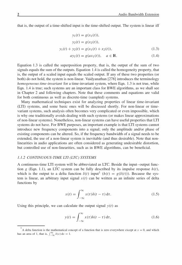
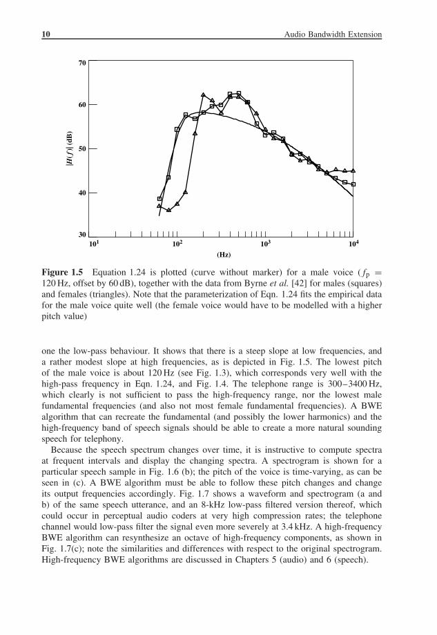
Figure 1.5 Equation 1.24 is plotted (curve without marker) for a male voice (fp =120 Hz, offset by 60 dB), together with the data from Byrne et al. [42] for males (squares)and females (triangles). Note that the parameterization of Eqn. 1.24 fits the empirical datafor the male voice quite well (the female voice would have to be modelled with a higherpitch value)
one the low-pass behaviour. It shows that there is a steep slope at low frequencies, anda rather modest slope at high frequencies, as is depicted in Fig. 1.5. The lowest pitchof the male voice is about 120 Hz (see Fig. 1.3), which corresponds very well with thehigh-pass frequency in Eqn. 1.24, and Fig. 1.4. The telephone range is 300–3400 Hz,which clearly is not sufficient to pass the high-frequency range, nor the lowest malefundamental frequencies (and also not most female fundamental frequencies). A BWEalgorithm that can recreate the fundamental (and possibly the lower harmonics) and thehigh-frequency band of speech signals should be able to create a more natural soundingspeech for telephony.
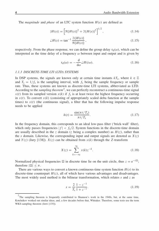
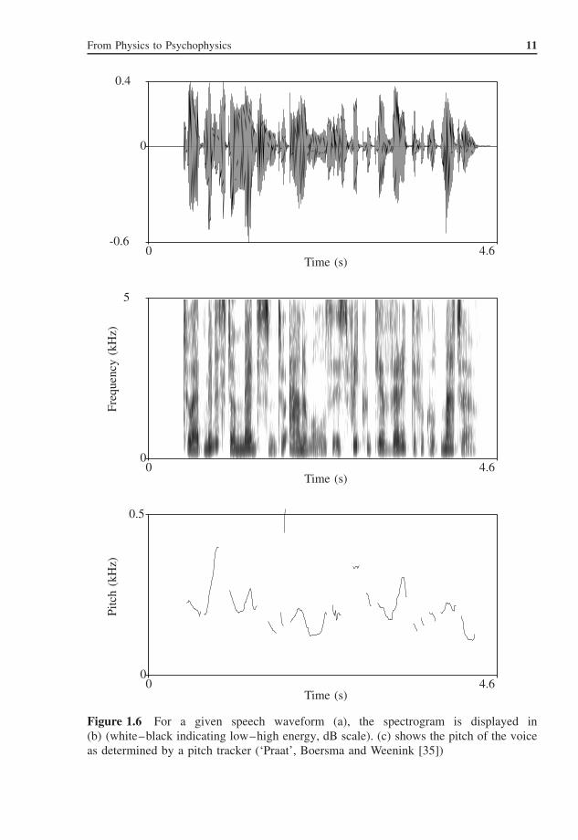
Because the speech spectrum changes over time, it is instructive to compute spectraat frequent intervals and display the changing spectra. A spectrogram is shown for aparticular speech sample in Fig. 1.6 (b); the pitch of the voice is time-varying, as can beseen in (c). A BWE algorithm must be able to follow these pitch changes and changeits output frequencies accordingly. Fig. 1.7 shows a waveform and spectrogram (a andb) of the same speech utterance, and an 8-kHz low-pass filtered version thereof, whichcould occur in perceptual audio coders at very high compression rates; the telephonechannel would low-pass filter the signal even more severely at 3.4 kHz. A high-frequencyBWE algorithm can resynthesize an octave of high-frequency components, as shown inFig. 1.7(c); note the similarities and differences with respect to the original spectrogram.High-frequency BWE algorithms are discussed in Chapters 5 (audio) and 6 (speech).
From Physics to Psychophysics 11
0.4
00
00
0
0-0.6
Time (s)
Time (s)
Time (s)
4.6
4.6
4.6
5
Freq
uenc
y(k
Hz)
0.5
Pitc
h(k
Hz)
Figure 1.6 For a given speech waveform (a), the spectrogram is displayed in(b) (white–black indicating low–high energy, dB scale). (c) shows the pitch of the voiceas determined by a pitch tracker (‘Praat’, Boersma and Weenink [35])

12 Audio Bandwidth Extension
0 0.5 1 1.5 2 2.5 3 3.5 4−1
−0.5
0
0.5
1
Time (s)
Am
plitu
de
0 0.5 1 1.5 2 2.5 3 3.5 4Time (s)
Fre
quen
cy (
Hz)
0.001
1
2
0 0.5 1 1.5 2 2.5 3 3.5 4Time (s)
Fre
quen
cy (
Hz)
0.001
1
2
0 0.5 1 1.5 2 2.5 3 3.5 4Time (s)
Fre
quen
cy (
Hz)
0.001
1
2
(d)
(c)
(b)
(a)
Figure 1.7 High-frequency BWE for a female voice (waveform in a, spectrogram in b)that has been low-pass filtered at 8 kHz (spectrogram in c). The processed signal (extendedto 16 kHz) is displayed as a spectrogram in d

From Physics to Psychophysics 13
1.2.2 MUSIC
More than 70 years ago, Sivian et al. [248] performed a pioneering study of musical spec-tra using live musicians and – for that time – innovative electronic measurement equip-ment. Shortly after the introduction of the CD, this study was repeated by Greiner andEggers [99] by using modern digital equipment and modern source material, at that timeCDs. The result of both studies was a series of graphs showing for each instrument orensemble the spectral amplitude distribution of the performed musical passage. The find-ings were that, in general, musical spectra have a bandpass characteristic, the exact shapeof which is determined by the music and the instrument. As in speech, the fundamentalfrequency (pitch) is time varying. A complicating factor is that various instruments maybe playing together, creating a superposition of several complex tones.
An example is shown in Fig. 1.8, where the variable time–frequency characteristic ofa 10-s excerpt of music is shown (‘One’, by Metallica). The waveform is shown in (a),and (b) shows a spectrogram (frequencies 0–140 Hz) of the original signal. The energyextends down to about 40 Hz. By using a low-frequency physical BWE algorithm, wecan extend this lower limit to about 20 Hz (c), which requires a subwoofer of excellentquality for correct reproduction. Because the resulting synthetic frequencies have similarspectro-temporal characteristics as the original low frequencies, they will be perceivedas an integral part of the signal (lowering the pitch of the bass tones to 20 Hz). Becauseof the very low frequencies that are now being radiated, it will also add ‘feeling’ to themusic. Low-frequency physical BWE algorithms are discussed in Chapter 3.
Another study (Fielder and Benjamin [70]) was conducted to establish design criteriafor the performance of subwoofers to be used for the reproduction of music in homes. Thefocus on subwoofers was motivated by the fact that low frequencies play an importantrole in the musical experience. A first conclusion of that study was that recordings withaudible bass below 30 Hz are relatively rare. Second, these very low frequencies weregenerated by pipe organs, synthesizers, or special effects and environmental noise. Otherinstruments, such as bass guitar, bass viol, tympani, or bass drum, produce relatively littleoutput below 40 Hz, although they may have very high levels at or above that frequency.Fielder and Benjamin [70] gave an example that for an average listening room of 68 m3,the required acoustic power for reproduction is 0.0316 W (which yields a sound pressurelevel of 97 dB), which requires a volume displacement of 0.685 l at 20 Hz. This requires anexcursion of 13.5 mm for a 10 in. (0.25 m) woofer. These are extraordinary requirements,and very hard to fulfil in practice. An alternative is to use low-frequency psychoacousticBWE methods, where frequencies that are too low to reproduce are shifted to higherfrequencies, in such a way that the pitch percept remains the same. These methods arediscussed in Chapter 2. If we consider Fig. 1.8 (c) as the original signal, we could thinkof such BWE as shifting the frequency band 20–40 Hz to above 40 Hz. The spectrogramof the resulting signal would resemble that of Fig. 1.8(b).
1.3 LOUDSPEAKERS
1.3.1 INTRODUCTION TO ACOUSTICS
BWE methods are closely related to acoustics, particularly acoustics of loudspeakers,so here we will review some basic concepts in this area. Extensive and more general

14 Audio Bandwidth Extension
0 1 2 3 4 5 6 7 8 9 10−1
−0.5
0
0.5
1
Time (s)
0 1 2 3 4 5 6 7 8 9 10
Time (s)
0 1 2 3 4 5 6 7 8 9 10
Time (s)
Am
plitu
deF
requ
ency
(H
z)
20
40
60
80
100
120
Fre
quen
cy (
Hz)
20
40
60
80
100
120
Figure 1.8 A 10-s excerpt of music (a), and its spectrogram for frequencies 0–140 Hz(b), which shows that the lowest frequencies contained in the signal are around 40 Hz. Alow-frequency physical BWE algorithm can extend this low-frequency spectrum down toabout 20 Hz, as shown in (c). Because the additional frequency components have a properharmonic relation with the original frequency components, and have a common temporalmodulation, they will be perceived as part of the original sound. In this case, the pitch ofthe bass notes will be lowered to 20 Hz

From Physics to Psychophysics 15
treatments of acoustics can be found in textbooks such as Kinsler et al. [142], Pierce[208], Beranek [28], Morse and Ingard [180]. Acoustics can be defined as the generation,transmission, and reception of energy in the form of vibrational waves in matter. As theatoms or molecules of a fluid or solid are displaced from their normal configurations,an internal elastic restoring force arises. Examples include the tensile force arising whena spring is stretched, the increase in pressure in a compressed fluid, and the transverserestoring force of a stretched wire that is displaced in a direction normal to its length. Itis this elastic restoring force, together with the inertia of the system, that enables matterto exhibit oscillatory vibrations, and thereby generate and transmit acoustic waves. Thosewaves that produce the sensation of sound are of a variety of pressure disturbances thatpropagate through a compressible fluid.
1.3.1.1 The Wave Equation
The wave equation gives the relation between the spatial (r) and temporal (t) derivatesof pressure p(r, t) as
2p(r, t) = 1
c2
∂2p(r, t)
∂t2(1.25)
where c is the speed of sound, which for air at 293 K is 343 m/s. Equation 1.25 is thelinearized, loss-less wave equation for the propagation of sounds in linear inviscid fluids.As a special case of the wave equation, we can consider the one-dimensional case, wherethe acoustic variables are only a function of one spatial coordinate, say along the x
direction. Equation 1.25 then reduces to
∂2p(x, t)
∂x2 = 1
c2
∂2p(x, t)
∂t2 . (1.26)
The solution of this equation yields two wave fields propagating in ±x directions, whichare called plane (progressive) waves. Sound waves radiated by a loudspeaker are consid-ered to be plane waves in the ‘far field’.
1.3.1.2 Acoustic Impedance
The ratio of acoustic pressure in a medium to the associated particle velocity is called thespecific acoustic impedance4 z(r)
z(r) = p(r)u(r)
. (1.27)
For plane progressive waves (Eqn. 1.26), this becomes
z = ρ0 c, (1.28)
independent of x, where ρ is the density of the fluid, being 1.21 kg/m3 for air at 293 K.
4Similar to Ohm’s law for electrical circuits.

16 Audio Bandwidth Extension
Table 1.1 Typical sounds and their cor-responding SPL values (dB)
Threshold of hearing 0Whispering 20Background noise at home 40Normal talking 60Noise pollution level 90Pneumatic drill at 5 m 1001 m from a loudspeaker at a disco 120Threshold of pain 140
1.3.1.3 Decibel Scales
Because of the large range of acoustical quantities, it is customary to express values ina logarithmic way. For sound pressure, we define the sound pressure level (SPL) Lp interms of decibel (dB), as
Lp = 20 log(p/p0), (1.29)
where p0 is a reference level (the log is base 10, as will be used throughout the book), forair p0 = 20 µPa is used. This level is chosen such that it corresponds to the just-noticeablesound pressure level of a 2-kHz sinusoid for an 18-year-old person with normal hearing,see Fig. 1.18 and ISO 226-1987(E) [117]. Table 1.1 lists some typical sounds and theircorresponding SPL values. It is convenient to memorize some dB values for the ratio’s√
2/2, 2, 10, and 30 as approximately 3, 6, 20, and 30 dB.
1.3.2 LOUDSPEAKERS
1.3.2.1 Electrodynamic Loudspeakers
Electroacoustic loudspeakers have been around for quite some time. While the first patentfor a moving-coil loudspeaker was filed in 1877, by Cuttriss and Redding [55], shortlyafter Bell’s [27] telephone invention, the real impetus to a commercial success was givenby Rice and Kellog [223] through their famous paper, so that we can state that theclassical electrodynamic loudspeaker as we know now (depicted in Fig. 1.10), is over80 years old. All practical electroacoustical transducers are limited in their capabilities,owing to their size and excursion possibilities. Among those limitations, there is one inthe frequency response, which will be the main topic in the following sections. To studythese limitations, we will scrutinize the behaviour of transducers for various parameters.It will appear later that the ‘force factor’ (Bl) of a loudspeaker plays an important role.To have some qualitative impression regarding the band limitation, various curves areshown in Fig. 1.9. We clearly see that there is a band-pass behaviour of the acousticalpower Pa (fifth curve in Fig. 1.9), and a high-pass response for the on-axis pressure p
(third curve in Fig. 1.9).First, we will discuss the efficiency of electrodynamic loudspeakers in general, which
will be used in a discussion about a special driver with a very low Bl value in Sec. 4.3.This driver can be made very cost efficient, low weight, flat, and with high power

From Physics to Psychophysics 17
−2
+1
+4
−1
+2
−2
wtw0Frequency
x
v
a, p
Re{Zrad}
Pa
+2
Stiffnesscontrol
Masscontrol
Figure 1.9 The displacement x, velocity v, acceleration a, together with the on-axispressure p, the real part of the radiation impedance �{Zrad}, and the acoustical powerPa of a rigid-plane piston in an infinite baffle, driven by a constant force. The numbersdenote the slopes of the curves; multiplied by 6, these yield the slope in dB/octave
efficiency. But first (Sec. 1.3.2.3), we show that sound reproduction at low frequencieswith small transducers, and at a reasonable efficiency, is very difficult. The reasons forthis are that the efficiency is inversely proportional to the moving mass and proportionalto the square of the product of cone area and force factor Bl.
1.3.2.2 Construction
An electrodynamic loudspeaker, of the kind depicted in Fig. 1.10, consists of a conicaldiaphragm, the cone, usually made of paper, being suspended by an outer suspensiondevice, or rim, and an inner suspension device, or spider. The suspension limits themaximum excursion of the cone so that the voice coil remains inside the air gap of thepermanent magnet. This limitation can lead to non-linear distortion; see for example,Tannaka et al. [264], Olson [193], Klippel [143, 144], Kaizer [140]. The voice coil isattached to the voice coil cylinder, generally made of paper or metal, which is glued tothe inner edge of the cone. In most cases, the spider is also attached to this edge. The voicecoil is placed in the radial magnetic field of a permanent magnet and is fed with the signalcurrent of the amplifier. For low frequencies, the driver can be modelled in a relativelysimple way, as it behaves as a rigid piston. In the next section the electronic behavior of thedriver will be described on the basis of a lumped-element model in which the mechanicaland acoustical elements can be interpreted in terms of the well-known properties of

18 Audio Bandwidth Extension
Permanent magnet
Voice coil
Frame Outer cone suspension (rim)
Cone
Inner cone suspension (spider)
Dust cap
Figure 1.10 Cross section of an electrodynamic cone loudspeaker
their analogous electronic-network counterparts. At higher frequencies (above the conebreak-up frequency), deviations from this model occur, as the driver’s diaphragm is thenno longer rigid. Both transverse and longitudinal waves then appear in the conical shell.These waves are coupled and together they determine the vibration pattern, which has aconsiderable effect on the sound radiation. Although this is an important issue, it will notbe considered here (see e.g. Kaizer [140], Frankort [75], van der Pauw [282]).
An alternative construction method is to have the voice coil stationary, and a movingmagnet; this will be discussed in Sec. 4.3.1.
1.3.2.3 Lumped-element Model
For low frequencies, a loudspeaker can be modelled with the aid of some simple elements,allowing the formulation of some approximate analytical expressions for the loudspeakersound radiation due to an electrical input current, or voltage, which proves to be quitesatisfactory for frequencies below the cone break-up frequency. The extreme acceler-ations experienced by a typical paper cone above about 2 kHz, cause it to flex in acomplex pattern. The cone no longer acts as a rigid piston but rather as a collection ofvibrating elements.
The forthcoming loudspeaker model will not be extensively derived here, as that hasbeen done elsewhere; see for example, Olson [192], Beranek [28], Borwick [36], Merhaut[173], Thiele [268], Small [252], Clark [51]. We first reiterate briefly the theory for thesealed loudspeaker. In what follows, we use a driver model with a simple acoustic airload. Beranek [28] shows that for a baffled piston this air load is a mass of air equivalentto 0.85a in thickness on each side of a piston of radius a. In fact, the air load can exceedthis value, since most drivers have a support basket, which obstructs the flow of air fromthe back of the cone, forcing it to move through smaller openings. This increases theacceleration of this air, augmenting the acoustic load.
From Physics to Psychophysics 19
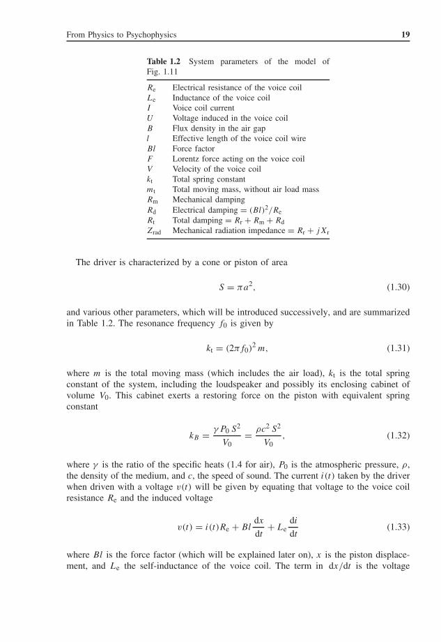
Table 1.2 System parameters of the model ofFig. 1.11
Re Electrical resistance of the voice coilLe Inductance of the voice coilI Voice coil currentU Voltage induced in the voice coilB Flux density in the air gapl Effective length of the voice coil wireBl Force factorF Lorentz force acting on the voice coilV Velocity of the voice coilkt Total spring constantmt Total moving mass, without air load massRm Mechanical dampingRd Electrical damping = (Bl)2/ReRt Total damping = Rr + Rm + RdZrad Mechanical radiation impedance = Rr + jXr
The driver is characterized by a cone or piston of area
S = πa2, (1.30)
and various other parameters, which will be introduced successively, and are summarizedin Table 1.2. The resonance frequency f0 is given by
kt = (2πf0)2 m, (1.31)
where m is the total moving mass (which includes the air load), kt is the total springconstant of the system, including the loudspeaker and possibly its enclosing cabinet ofvolume V0. This cabinet exerts a restoring force on the piston with equivalent springconstant
kB = γP0 S2
V0= ρc2 S2
V0, (1.32)
where γ is the ratio of the specific heats (1.4 for air), P0 is the atmospheric pressure, ρ,the density of the medium, and c, the speed of sound. The current i(t) taken by the driverwhen driven with a voltage v(t) will be given by equating that voltage to the voice coilresistance Re and the induced voltage
v(t) = i(t)Re + Bldx
dt+ Le
di
dt(1.33)
where Bl is the force factor (which will be explained later on), x is the piston displace-ment, and Le the self-inductance of the voice coil. The term in dx/dt is the voltage

20 Audio Bandwidth Extension
induced by the driver piston velocity of motion. Using the Laplace transform, Eqn. 1.33can be written as
V (s) = I (s)Re + BlsX(s) + LesI (s), (1.34)
where capitals are used for the Laplace-transformed variables, and s is the Laplace vari-able, which can be replaced by iω for stationary harmonic signals. The relation betweenthe mechanical forces and the electrical driving force is given by
md2x
dt2 + Rmdx
dt+ ktx = Bli, (1.35)
where at the left-hand side, we have the mechanical forces, which are the inertial reactionof the cone with mass m, the mechanical resistance Rm, and the total spring force withtotal spring constant kt; at the right-hand side, we have the external electromagneticLorentz force F = Bli acting on the voice coil, with B, the flux density in the air gap, i,the voice coil current, and l being the effective length of the voice coil wire. CombiningEqns. 1.34 and 1.35, we get
X(s)
[s2 m + s(Rm + (Bl)2
Les + Re+ kt
]= BlV (s)
Les + Re. (1.36)
We see that besides the mechanical damping Rm, we also get an electrical damping term(Bl)2/(Les + Re), and this term plays an important role. If we ignore the inductance ofthe loudspeaker, the effect of eddy currents5 induced in the pole structure (Vanderkooy[283]), and the effect of creep6, we can write Eqn. 1.36 as the transfer function Hx(s)
between voltage and excursion
Hx(s) = X(s)
V (s)= Bl/Re
s2 m + s(R + (Bl)2/Re) + kt. (1.37)
We use an infinite baffle to mount the piston, and in the compact-source regime (a/r �c/(ωa)) the far-field acoustic pressure p(t) a distance r away becomes
p(t) = ρS( d2x/ dt2)/(2πr), (1.38)
proportional to the volume acceleration of the source (Morse and Ingard [180], Kinsleret al. [142]). In the Laplace domain, we have
P(s) = s2ρSX(s)/(2πr). (1.39)
5Owing to the eddy current losses in the voice coil, the voice coil does not behave as an ideal coil, but it can
be modelled very well by means of Le = L0(1 − jα), where α is in the order of magnitude of 0.5.6
With a voltage or current step as the input, the displacement would be expected to reach its steady-state valuein a fraction of a second, according to the traditional model. The displacement may, however, continue to increase.This phenomenon is called creep. Creep is due the viscoelastic effects (Knudsen and Jensen [145], Flugge [74])of the spring (spider) and edge of the loudspeaker’s suspension.
From Physics to Psychophysics 21
+
−
Filter Lumped impedance model
C
ZradE
Re Le Rmmt
U = Bl V
–F = Bl I
Vkt
1
U FI
L
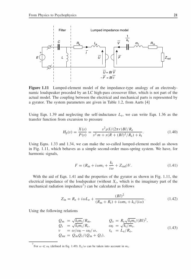
Figure 1.11 Lumped-element model of the impedance-type analogy of an electrody-namic loudspeaker preceded by an LC high-pass crossover filter, which is not part of theactual model. The coupling between the electrical and mechanical parts is represented bya gyrator. The system parameters are given in Table 1.2, from Aarts [4]
Using Eqn. 1.39 and neglecting the self-inductance Le, we can write Eqn. 1.36 as thetransfer function from excursion to pressure
Hp(s) = X(s)
P (s)= s2ρS/(2πr)Bl/Re
s2 m + s(R + (Bl)2/Re) + kt. (1.40)
Using Eqns. 1.33 and 1.34, we can make the so-called lumped-element model as shownin Fig. 1.11, which behaves as a simple second-order mass-spring system. We have, forharmonic signals,
F = (Rm + iωmt + kt
iω+ Zrad)V . (1.41)
With the aid of Eqn. 1.41 and the properties of the gyrator as shown in Fig. 1.11, theelectrical impedance of the loudspeaker (without Xr, which is the imaginary part of themechanical radiation impedance7) can be calculated as follows
Zin = Re + iωLe + (Bl)2
(Rm + Rr) + iωmt + kt/(iω). (1.42)
Using the following relations
Qm = √ktmt/Rm, Qe = Re
√ktmt/(Bl)2,
Qr = √ktmt/Rr, ω0 = √
kt/mt,
ν = ω/ω0 − ω0/ω, τe = Le/Re,
Qmr = QmQr/(Qm + Qr),
(1.43)
7For ω � ωt (defined in Eq. 1.49) Xr/ω can be taken into account in mt.

22 Audio Bandwidth Extension
1 × 100
1 × 10⁻¹
1 × 10⁻³
1 × 10⁻²
1 × 10⁻⁴
1 × 10⁻² 1 × 10⁻¹ 1 × 1011 × 100
ka
Zra
d/r
cpa2
Figure 1.12 Real (dashed line) and imaginary (solid line) parts of the normalized radi-ation impedance of a rigid disk with a radius a in an infinite baffle
we can write Zin as
Zin = Re
[1 + iωτe + Qmr/Qe
1 + iQmrν
], (1.44)
if we neglect Le, we get at the resonance frequency (ν = 0) the maximal input impedance
Zin(ω = ω0) = Re(1 + Qmr/Qe) ≈ Re + (Bl)2/Rm. (1.45)
The time-averaged electrical power Pe delivered to the driver is then
Pe = 0.5|I |2�{Zin} = 0.5|I |2Re
[1 + Qmr/Qe
1 + Q2mrν
2
]. (1.46)
The radiation impedance of a plane-circular rigid piston8 with a radius a in an infinitebaffle can be derived as (Morse and Ingard [180, p. 384])
Zrad = πa2ρc[1 − 2J1(2 ka)/(2 ka) + i2H1(2 ka)/(2 ka)], (1.47)
where H1 is a Struve function (Abramowitz and Stegun [12, 12.1.7]), J1 is a Besselfunction and k is the wave number ω/c. The real and imaginary parts of Zrad are plottedin Fig. 1.12.
8The radiation impedance of rigid cones and that of rigid domes is studied in, for example, Suzuki and Tichy
[259, 260]. They appeared to be significantly different with respect to rigid pistons for ka > 1, revealing that Zradfor convex domes is generally lower than that for pistons and higher than that for concave domes.
From Physics to Psychophysics 23
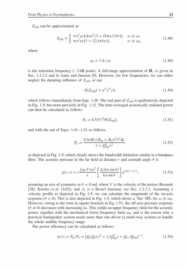
Zrad can be approximated as
Zrad ≈{
πa2ρc[(ka)2/2 + i8 ka/(3π)], ω � ωt
πa2ρc[1 + i2/(πka)], ω � ωt,(1.48)
where
ωt = 1.4 c/a (1.49)
is the transition frequency (−3 dB point). A full-range approximation of H1 is given inSec. 1.3.3.2 and in Aarts and Janssen [9]. However, for low frequencies, we can eitherneglect the damping influence of Zrad, or use
�{Zrad} ≈ a4f 2/4, (1.50)
which follows immediately from Eqn. 1.48. The real part of Zrad is qualitatively depictedin Fig. 1.9, but more precisely in Fig. 1.12. The time-averaged acoustically radiated powercan then be calculated as follows
Pa = 0.5|V |2�{Zrad}, (1.51)
and with the aid of Eqns. 1.41–1.51 as follows
Pa = 0.5(Bl/(Rm + Rr))2I 2Rr
1 + Q2mrν
2, (1.52)
as depicted in Fig. 1.9, which clearly shows the bandwidth limitation similar to a bandpassfilter. The acoustic pressure in the far field at distance r and azimuth angle θ is
p(r, t) = ifρ0 V πa2
r
[J1(ka sin θ)
ka sin θ
]eiω(t−r/c), (1.53)
assuming an axis of symmetry at θ = 0 rad, where V is the velocity of the piston (Beranek[28], Kinsler et al. [142]), and J1 is a Bessel function, see Sec. 1.3.3.1. Assuming avelocity profile as depicted in Fig. 1.9, we can calculate the magnitude of the on-axisresponse (θ = 0). This is also depicted in Fig. 1.9, which shows a ‘flat’ SPL for ω � ω0.However, owing to the term in square brackets in Eq. 1.53, the off-axis pressure response(θ �= 0) decreases with increasing ka. This yields an upper frequency limit for the acousticpower, together with the mechanical lower frequency limit ω0, and is the reason why apractical loudspeaker system needs more than one driver (a multi-way system) to handlethe whole audible frequency range.
The power efficiency can be calculated as follows
η(ν) = Pa/Pe = [QeQr(ν2 + 1/Q2
mr) + Qr/Qmr]−1. (1.54)

24 Audio Bandwidth Extension
In Fig. 4.13, some plots for η(ν) for various drivers are shown. For low frequencies9, sothat Qmr ≈ Qm, the efficiency can be approximated as
η(ν) = Pa/Pe ≈ [Qr{Qe(ν2 + 1/Q2
m) + 1/Qm}]−1. (1.55)
A convenient way to relate the sound pressure level Lp to the power efficiency η is thefollowing. For a plain wave, we have the relation between sound intensity I and soundpressure p
I = p2
ρc, (1.56)
and the acoustical power is equal to
Pa = 2πr2I (1.57)
or
Pa = 2πr2p2
ρc. (1.58)
Using the above relations, we get
Lp = 20 log
(√Paρc
2πr2/p0
), (1.59)
where we assume radiation into one hemifield (solid angle of 2π), that is, we only accountfor the pressure at one side of the cone, which is mounted in an infinite baffle. For r = 1 m,ρ = 415, Pa = 1 W, and p0 = 20 10−6, we get
Lp = 112 + log η . (1.60)
If η = 1 (in this case Pa = Pe = 1 W), we get the maximum attainable Lp of 112 dB.Equation 1.60 can also be used to calculate η if Lp is known, for example, bymeasurement.
1.3.3 BESSEL AND STRUVE FUNCTIONS
Bessel and Struve functions occur in many places in physics and quite prominently inacoustics for impedance calculations. The problem of the rigid-piston radiator mountedin an infinite baffle has been studied widely for tutorial as well as for practical reasons,see for example, Greenspan [98], Pierce [208], Kinsler et al. [142], Beranek [28], Morseand Ingard [180]. The resulting theory is commonly applied to model a loudspeaker inthe audio-frequency range. For a baffled piston, the ratio of the force amplitude to the
9It should be noted that Qr depends on ω, but using Eqns. 1.43 and 1.48 for ω � ωt, we can approximate
Qr ≈ 2 c√
ktmt/(πa4ρω2).
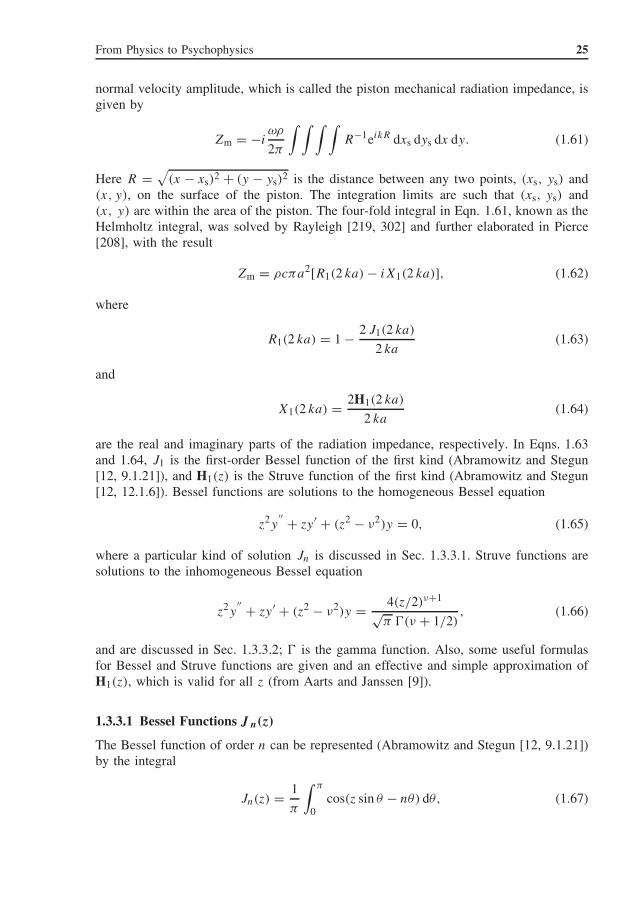
From Physics to Psychophysics 25
normal velocity amplitude, which is called the piston mechanical radiation impedance, isgiven by
Zm = −iωρ
2π
∫ ∫ ∫ ∫R−1eikR dxs dys dx dy. (1.61)
Here R =√
(x − xs)2 + (y − ys)2 is the distance between any two points, (xs, ys) and(x, y), on the surface of the piston. The integration limits are such that (xs, ys) and(x, y) are within the area of the piston. The four-fold integral in Eqn. 1.61, known as theHelmholtz integral, was solved by Rayleigh [219, 302] and further elaborated in Pierce[208], with the result
Zm = ρcπa2[R1(2 ka) − iX1(2 ka)], (1.62)
where
R1(2 ka) = 1 − 2 J1(2 ka)
2 ka(1.63)
and
X1(2 ka) = 2H1(2 ka)
2 ka(1.64)
are the real and imaginary parts of the radiation impedance, respectively. In Eqns. 1.63and 1.64, J1 is the first-order Bessel function of the first kind (Abramowitz and Stegun[12, 9.1.21]), and H1(z) is the Struve function of the first kind (Abramowitz and Stegun[12, 12.1.6]). Bessel functions are solutions to the homogeneous Bessel equation
z2y′′ + zy′ + (z2 − ν2)y = 0, (1.65)
where a particular kind of solution Jn is discussed in Sec. 1.3.3.1. Struve functions aresolutions to the inhomogeneous Bessel equation
z2y′′ + zy′ + (z2 − ν2)y = 4(z/2)ν+1
√π (ν + 1/2)
, (1.66)
and are discussed in Sec. 1.3.3.2; is the gamma function. Also, some useful formulasfor Bessel and Struve functions are given and an effective and simple approximation ofH1(z), which is valid for all z (from Aarts and Janssen [9]).
1.3.3.1 Bessel Functions J n(z)
The Bessel function of order n can be represented (Abramowitz and Stegun [12, 9.1.21])by the integral
Jn(z) = 1
π
∫ π
0cos(z sin θ − nθ) dθ, (1.67)

26 Audio Bandwidth Extension
0 5 10 15 20 25−0.4
−0.2
0
0.2
0.4
0.6
0.8
1
Figure 1.13 Plot of Bessel functions J0(x) (dashed), and J1(x) (solid)
and is plotted in Fig. 1.13 for n = 0, 1. There is the power series expansion (Abramowitzand Stegun [12, 9.1.10])
Jn(z) =( z
2
)n∞∑
k=0
(−z2
4
)k
k! (n + k + 1), (1.68)
which yields
J0(z) = 1 −14z2
(1!)2+
(14z2
)2
(2!)2−
(14z2
)3
(3!)2+ · · · , (1.69)
and
J1(z) = z
2− z3
16+ z5
384− z7
18 432+ · · · . (1.70)
For the purpose of numerical computation, these series are only useful for small valuesof z. For small values of z, Eqns. 1.63 and 1.70 yield
R1(ka) ≈ (ka)2
2, (1.71)
where we have substituted ka = z; this is in agreement with the small ka approximationas can be found in the references given earlier, see also Fig. 1.12. Furthermore, there is

From Physics to Psychophysics 27
the asymptotic result (Abramowitz and Stegun [12, 9.2.1 with ν = 1]), see Fig. 1.13,
J1(z) =√
2
πz(cos(z − 3π/4) + O(1/z)) , z → ∞, (1.72)
but this is only useful for large values of z. Equation 1.63 and the first term of Equation 1.72yield for large values of z (again substituting ka)
R1(ka) ≈ 1, (1.73)
which is in agreement with the large ka approximation, as can be found in the givenreferences as well. The function Jn(x) is tabulated in many books (see e.g. Abramowitzand Stegun [12]), and many approximation formulas exist (see e.g. Abramowitz andStegun [12, 9.4]). Another method to evaluate Jn is to use the following recurrent relation
Jn−1(x) + Jn+1(x) = 2n
xJn(x), (1.74)
provided that n < x, otherwise severe accumulation of rounding errors will occur(Abramowitz and Stegun [12, 9.12]). However, Jn(x) is always a decreasing functionof n when n > x, so the recurrence can always be carried out in the direction of decreas-ing n. The iteration is started with an arbitrary value zero for Jn, and unity for Jn−1. Wenormalize the results by using the equation
J0(x) + 2J2(x) + 2J4(x) + · · · = 1. (1.75)
A heuristic formula to determine the value of m to start the recurrence with Jm = 1 andJm−1 = 0 is (�·� indicates rounding to the nearest integer)
m =⌈
6 + max(n, p) + 9pp+2
2
⌋
p = 3x
2. (1.76)
1.3.3.2 The Struve Function H1(z)
The first-order Struve function H1(z) is defined as
H1(z) = 2z
π
∫ 1
0
√1 − t2 sin zt dt (1.77)
and is plotted in Fig. 1.14. There is the power series expansion (Abramowitz and Stegun[12, 12.1.5])
H1(z) = 2
π
[z2
123− z4
12325+ z6
1232527− · · ·
]. (1.78)

28 Audio Bandwidth Extension
0 5 10 15 20 250
0.2
0.4
0.6
0.8
1
Figure 1.14 Plot of Struve function H1(x)
For the purpose of numerical computation, this series is only useful for small valuesof z. Eqns. 1.64 and 1.78 yield, for small values of z (substituting ka for z)
X1(ka) ≈ 8 ka
3π, (1.79)
which is in agreement with the small ka approximation as can be found in the referencesgiven earlier, see also Fig. 1.12. Furthermore, there is the asymptotic result (Abramowitzand Stegun [12, 12.1.31, 9.2.2 with ν = 1]).
H1(z) = 2
π−
√2
πz(cos(z − π/4) + O(1/z)) , z → ∞, (1.80)
but this is only useful for large values of z. Eqn. 1.64 and the first term of Eqn. 1.80yield for large values of ka
X1(ka) ≈ 2
πka, (1.81)
which is in agreement with the large ka approximation, as can also be found in the earliergiven references. An approximation for all values of ka was developed by Aarts andJanssen [9]. Here, only a limited number of elementary functions is involved:
H1(z) ≈ 2
π− J0(z) +
(16
π− 5
)sin z
z+
(12 − 36
π
)1 − cos z
z2. (1.82)
The approximation error is small and decently spread out over the whole z-range, vanishesfor z = 0, and its maximum value is about 0.005. Replacing H1(z) in Fig. 1.12 by theapproximation in Eqn. 1.82 would result in no visible change. The maximum relativeerror appears to be less than 1%, equals 0.1% at z = 0, and decays to zero for z → ∞.

From Physics to Psychophysics 29
1.3.3.3 Example
A prime example of the use of the radiation impedance is for the calculation of theradiated acoustic power of a circular piston in an infinite baffle. This is an accurate modelfor a loudspeaker with radius a mounted in a large cabinet (Beranek [28]). The radiatedacoustic power is equal to
Pa = 0.5|V |2�{Zm}, (1.83)
where V is the velocity of the loudspeaker’s cone. The use of the just-obtained approx-imation for H1 is to calculate the loudspeaker’s electrical input impedance Zin, whichis a function of Zm (see Beranek [28]). Using Zin, the time-averaged electrical powerdelivered to the loudspeaker is calculated as
Pe = 0.5|I |2�{Zin}, (1.84)
where I is the current fed into the loudspeaker. Finally, the efficiency of a loudspeaker,defined as
η(ka) = Pa/Pe, (1.85)
can be calculated. These techniques are used in Chapter 4 when analyzing the behaviorof loudspeakers with special drivers.
1.4 AUDITORY PERCEPTION
This section reviews the basic concepts of the auditory system and auditory perception,insofar as they relate to BWE methods that will be discussed in later chapters. Thetreatment here is necessarily concise, but there are numerous references provided forfurther reading, if necessary or desired. Reviews of psychoacoustics can be found in, forexample, Moore [177, 178], Yost et al. [302]; physiology of the peripheral hearing systemis discussed in, for example, Geisler [86].
1.4.1 PHYSICAL CHARACTERISTICS OF THE PERIPHERAL HEARING SYSTEM
The peripheral hearing system consists of outer, middle, and inner ear, see Fig. 1.15.Sound first enters via the pinna, which has an irregular shape that filters impinging soundwaves. This feature aids in sound localization, which is not further discussed here (seee.g. Batteau [26], Blauert [34]). Next, sound passes into the auditory canal and on tothe eardrum, or tympanic membrane, which transmits vibrations in the air to the threemiddle ear bones, the ossicles (malleus, incus, and stapes). The stapes connects to the ovalwindow, the entrance to the fluid-filled cochlea. The system from tympanic membrane tooval window serves as an impedance-matching device so that a large portion of soundenergy at the frequencies of interest, in the air, is transmitted into the cochlea. Musclesconnect the malleus and stapes to the bone of the skull, and contraction of these muscles
30 Audio Bandwidth Extension
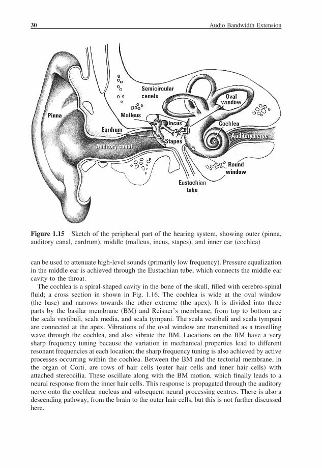
Figure 1.15 Sketch of the peripheral part of the hearing system, showing outer (pinna,auditory canal, eardrum), middle (malleus, incus, stapes), and inner ear (cochlea)
can be used to attenuate high-level sounds (primarily low frequency). Pressure equalizationin the middle ear is achieved through the Eustachian tube, which connects the middle earcavity to the throat.
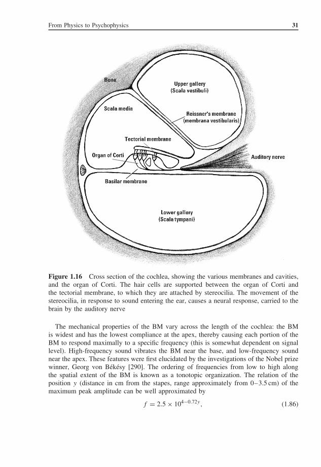
The cochlea is a spiral-shaped cavity in the bone of the skull, filled with cerebro-spinalfluid; a cross section in shown in Fig. 1.16. The cochlea is wide at the oval window(the base) and narrows towards the other extreme (the apex). It is divided into threeparts by the basilar membrane (BM) and Reisner’s membrane; from top to bottom arethe scala vestibuli, scala media, and scala tympani. The scala vestibuli and scala tympaniare connected at the apex. Vibrations of the oval window are transmitted as a travellingwave through the cochlea, and also vibrate the BM. Locations on the BM have a verysharp frequency tuning because the variation in mechanical properties lead to differentresonant frequencies at each location; the sharp frequency tuning is also achieved by activeprocesses occurring within the cochlea. Between the BM and the tectorial membrane, inthe organ of Corti, are rows of hair cells (outer hair cells and inner hair cells) withattached stereocilia. These oscillate along with the BM motion, which finally leads to aneural response from the inner hair cells. This response is propagated through the auditorynerve onto the cochlear nucleus and subsequent neural processing centres. There is also adescending pathway, from the brain to the outer hair cells, but this is not further discussedhere.
From Physics to Psychophysics 31
Figure 1.16 Cross section of the cochlea, showing the various membranes and cavities,and the organ of Corti. The hair cells are supported between the organ of Corti andthe tectorial membrane, to which they are attached by stereocilia. The movement of thestereocilia, in response to sound entering the ear, causes a neural response, carried to thebrain by the auditory nerve
The mechanical properties of the BM vary across the length of the cochlea: the BMis widest and has the lowest compliance at the apex, thereby causing each portion of theBM to respond maximally to a specific frequency (this is somewhat dependent on signallevel). High-frequency sound vibrates the BM near the base, and low-frequency soundnear the apex. These features were first elucidated by the investigations of the Nobel prizewinner, Georg von Bekesy [290]. The ordering of frequencies from low to high alongthe spatial extent of the BM is known as a tonotopic organization. The relation of theposition y (distance in cm from the stapes, range approximately from 0–3.5 cm) of themaximum peak amplitude can be well approximated by
f = 2.5 × 10⁴−0.72y, (1.86)
32 Audio Bandwidth Extension
6000 Hz
600 Hz
50 Hz
0 1 2
z (cm)Stapes Apex
3
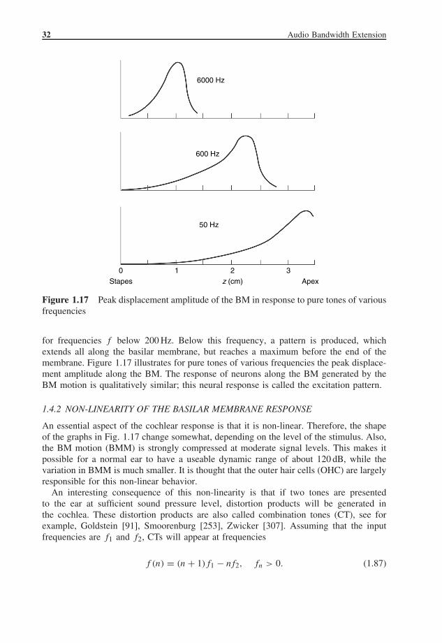
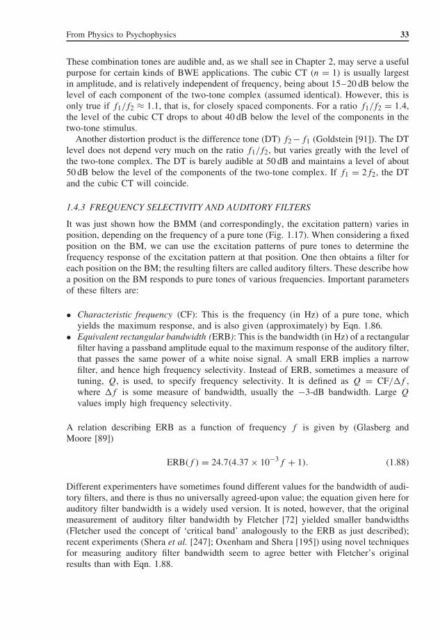
Figure 1.17 Peak displacement amplitude of the BM in response to pure tones of variousfrequencies
for frequencies f below 200 Hz. Below this frequency, a pattern is produced, whichextends all along the basilar membrane, but reaches a maximum before the end of themembrane. Figure 1.17 illustrates for pure tones of various frequencies the peak displace-ment amplitude along the BM. The response of neurons along the BM generated by theBM motion is qualitatively similar; this neural response is called the excitation pattern.
1.4.2 NON-LINEARITY OF THE BASILAR MEMBRANE RESPONSE
An essential aspect of the cochlear response is that it is non-linear. Therefore, the shapeof the graphs in Fig. 1.17 change somewhat, depending on the level of the stimulus. Also,the BM motion (BMM) is strongly compressed at moderate signal levels. This makes itpossible for a normal ear to have a useable dynamic range of about 120 dB, while thevariation in BMM is much smaller. It is thought that the outer hair cells (OHC) are largelyresponsible for this non-linear behavior.
An interesting consequence of this non-linearity is that if two tones are presentedto the ear at sufficient sound pressure level, distortion products will be generated inthe cochlea. These distortion products are also called combination tones (CT), see forexample, Goldstein [91], Smoorenburg [253], Zwicker [307]. Assuming that the inputfrequencies are f1 and f2, CTs will appear at frequencies
f (n) = (n + 1)f1 − nf2, fn > 0. (1.87)
From Physics to Psychophysics 33
These combination tones are audible and, as we shall see in Chapter 2, may serve a usefulpurpose for certain kinds of BWE applications. The cubic CT (n = 1) is usually largestin amplitude, and is relatively independent of frequency, being about 15–20 dB below thelevel of each component of the two-tone complex (assumed identical). However, this isonly true if f1/f2 ≈ 1.1, that is, for closely spaced components. For a ratio f1/f2 = 1.4,the level of the cubic CT drops to about 40 dB below the level of the components in thetwo-tone stimulus.
Another distortion product is the difference tone (DT) f2 −f1 (Goldstein [91]). The DTlevel does not depend very much on the ratio f1/f2, but varies greatly with the level ofthe two-tone complex. The DT is barely audible at 50 dB and maintains a level of about50 dB below the level of the components of the two-tone complex. If f1 = 2f2, the DTand the cubic CT will coincide.
1.4.3 FREQUENCY SELECTIVITY AND AUDITORY FILTERS
It was just shown how the BMM (and correspondingly, the excitation pattern) varies inposition, depending on the frequency of a pure tone (Fig. 1.17). When considering a fixedposition on the BM, we can use the excitation patterns of pure tones to determine thefrequency response of the excitation pattern at that position. One then obtains a filter foreach position on the BM; the resulting filters are called auditory filters. These describe howa position on the BM responds to pure tones of various frequencies. Important parametersof these filters are:
• Characteristic frequency (CF): This is the frequency (in Hz) of a pure tone, whichyields the maximum response, and is also given (approximately) by Eqn. 1.86.
• Equivalent rectangular bandwidth (ERB): This is the bandwidth (in Hz) of a rectangularfilter having a passband amplitude equal to the maximum response of the auditory filter,that passes the same power of a white noise signal. A small ERB implies a narrowfilter, and hence high frequency selectivity. Instead of ERB, sometimes a measure oftuning, Q, is used, to specify frequency selectivity. It is defined as Q = CF/�f ,where �f is some measure of bandwidth, usually the −3-dB bandwidth. Large Q
values imply high frequency selectivity.
A relation describing ERB as a function of frequency f is given by (Glasberg andMoore [89])
ERB(f ) = 24.7(4.37 × 10⁻³f + 1). (1.88)
Different experimenters have sometimes found different values for the bandwidth of audi-tory filters, and there is thus no universally agreed-upon value; the equation given here forauditory filter bandwidth is a widely used version. It is noted, however, that the originalmeasurement of auditory filter bandwidth by Fletcher [72] yielded smaller bandwidths(Fletcher used the concept of ‘critical band’ analogously to the ERB as just described);recent experiments (Shera et al. [247]; Oxenham and Shera [195]) using novel techniquesfor measuring auditory filter bandwidth seem to agree better with Fletcher’s originalresults than with Eqn. 1.88.

34 Audio Bandwidth Extension
A commonly used model for auditory filter shape is by means of the gammatone filter(Patterson et al. [204], Hohman [110]) gt(t)
gt(t) = atn−1e−2πb·ERB(fc)t cos(2πfct+φ). (1.89)
Here a, b, n, fc, and φ are parameters and ERB(fc) is as given in Eqn. 1.88. The gam-matone filters are often used in auditory models (e.g. AIM; see Sec. 1.4.8) to simulatethe spectral analysis performed by the BM.
The frequency selectivity of the auditory filters is thought to have a large influenceon many auditory tasks, such as understanding speech in noise or detecting small timbredifferences between sounds. For BWE applications, another interesting aspect of auditoryfilters is their presumed influence on pitch perception, discussed in Sec. 1.4.5. For themoment, we mention that depending on the ERB of an auditory filter, it may pass oneor more harmonics of a complex tone, also depending on the fundamental frequencyof that tone. It turns out that roughly up to harmonic number 10, auditory filters passonly one harmonic, that is, these harmonics are spectrally resolved . At higher harmonicnumbers, the ERB of the auditory filters become wider than the harmonic frequencyspacing, and therefore the auditory filters pass two or more harmonics. These harmonicsare thus spectrally unresolved, and the output of the auditory filter is a superposition ofa number of these higher harmonics. Whether a harmonic is resolved or not will havea large influence on the subsequently generated neural response. In the following, wewill alternately use the terms harmonic and partial, both referring to one component of aharmonically related complex tone.
1.4.4 LOUDNESS AND MASKING
1.4.4.1 Definitions
Loudness is related to the level, or amplitude, of a sound, but depends in a complicatedmanner on level and also frequency content. The following definitions are used by theISO [117]
Definition 4 Loudness: That attribute of auditory sensation in terms of which sounds maybe ordered on a scale extending from soft to loud. Loudness is expressed in sone, whereone sone is the loudness of a sound, whose loudness level is 40 phon.
Definition 5 Loudness level: Of a given sound, the sound pressure level of a referencesound, consisting of a sinusoidal plane progressive wave of frequency 1 kHz coming fromdirectly in front of the listener, which is judged by otologically normal persons to be equallyloud to the given sound. Loudness level is expressed in phon.
Definition 6 Critical bandwidth: The widest frequency band within which the loudness ofa band of continuously distributed random noise of constant band sound pressure level isindependent of its bandwidth.
Note that the critical bandwidth so defined is intimately related to the ERB of the auditoryfilters (Eqn. 1.88) and also Fletcher’s critical band.
From Physics to Psychophysics 35
Sou
nd p
ress
ure
leve
l (dB
)
Frequency (Hz)
−10
10
30
50
70
90
110
130
31,5 125 500 2000 8000
110 phon
100
90
80
70
60
50
40
30
20
10
MAF
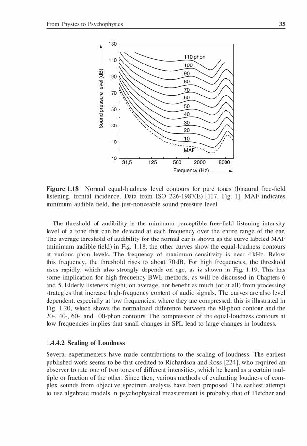
Figure 1.18 Normal equal-loudness level contours for pure tones (binaural free-fieldlistening, frontal incidence. Data from ISO 226-1987(E) [117, Fig. 1]. MAF indicatesminimum audible field, the just-noticeable sound pressure level
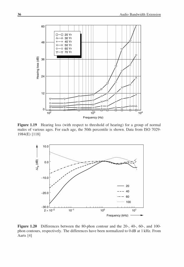
The threshold of audibility is the minimum perceptible free-field listening intensitylevel of a tone that can be detected at each frequency over the entire range of the ear.The average threshold of audibility for the normal ear is shown as the curve labeled MAF(minimum audible field) in Fig. 1.18; the other curves show the equal-loudness contoursat various phon levels. The frequency of maximum sensitivity is near 4 kHz. Belowthis frequency, the threshold rises to about 70 dB. For high frequencies, the thresholdrises rapidly, which also strongly depends on age, as is shown in Fig. 1.19. This hassome implication for high-frequency BWE methods, as will be discussed in Chapters 6and 5. Elderly listeners might, on average, not benefit as much (or at all) from processingstrategies that increase high-frequency content of audio signals. The curves are also leveldependent, especially at low frequencies, where they are compressed; this is illustrated inFig. 1.20, which shows the normalized difference between the 80-phon contour and the20-, 40-, 60-, and 100-phon contours. The compression of the equal-loudness contours atlow frequencies implies that small changes in SPL lead to large changes in loudness.
1.4.4.2 Scaling of Loudness
Several experimenters have made contributions to the scaling of loudness. The earliestpublished work seems to be that credited to Richardson and Ross [224], who required anobserver to rate one of two tones of different intensities, which he heard as a certain mul-tiple or fraction of the other. Since then, various methods of evaluating loudness of com-plex sounds from objective spectrum analysis have been proposed. The earliest attemptto use algebraic models in psychophysical measurement is probably that of Fletcher and
36 Audio Bandwidth Extension
Frequency (Hz)
102 103 1040
12
24
36
48
60
Hea
ring
loss
(dB
)20 Yr30 Yr40 Yr50 Yr60 Yr70 Yr
Figure 1.19 Hearing loss (with respect to threshold of hearing) for a group of normalmales of various ages. For each age, the 50th percentile is shown. Data from ISO 7029-1984(E) [118]
2 × 10⁻²−30.0
Frequency (kHz)
∆Lp
(dB
)
−20.0
−10.0
0.0
10.0
10−1 100 101
20
40
60
100
Figure 1.20 Differences between the 80-phon contour and the 20-, 40-, 60-, and 100-phon contours, respectively. The differences have been normalized to 0 dB at 1 kHz. FromAarts [4]
From Physics to Psychophysics 37
58
62
66
70
74
Bandwidth (Hz)
L (
phon
)
L (
dBA
)
100 1k 10k
60
62
66
70
74
Figure 1.21 Increasing loudness (solid curve) versus bandwidth of white noise, whilethe dB(A) Level (dashed line) was kept constant. From Aarts [4]
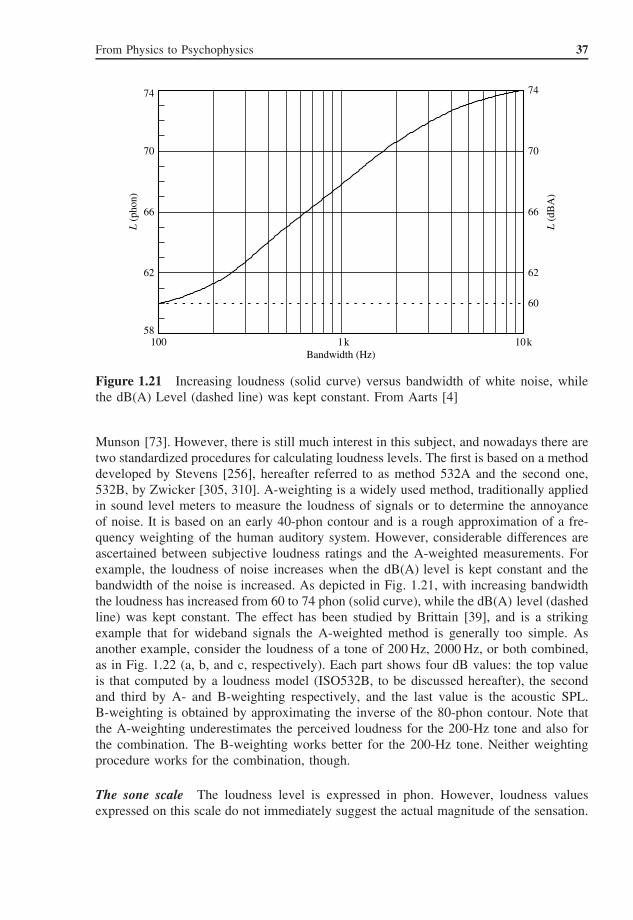
Munson [73]. However, there is still much interest in this subject, and nowadays there aretwo standardized procedures for calculating loudness levels. The first is based on a methoddeveloped by Stevens [256], hereafter referred to as method 532A and the second one,532B, by Zwicker [305, 310]. A-weighting is a widely used method, traditionally appliedin sound level meters to measure the loudness of signals or to determine the annoyanceof noise. It is based on an early 40-phon contour and is a rough approximation of a fre-quency weighting of the human auditory system. However, considerable differences areascertained between subjective loudness ratings and the A-weighted measurements. Forexample, the loudness of noise increases when the dB(A) level is kept constant and thebandwidth of the noise is increased. As depicted in Fig. 1.21, with increasing bandwidththe loudness has increased from 60 to 74 phon (solid curve), while the dB(A) level (dashedline) was kept constant. The effect has been studied by Brittain [39], and is a strikingexample that for wideband signals the A-weighted method is generally too simple. Asanother example, consider the loudness of a tone of 200 Hz, 2000 Hz, or both combined,as in Fig. 1.22 (a, b, and c, respectively). Each part shows four dB values: the top valueis that computed by a loudness model (ISO532B, to be discussed hereafter), the secondand third by A- and B-weighting respectively, and the last value is the acoustic SPL.B-weighting is obtained by approximating the inverse of the 80-phon contour. Note thatthe A-weighting underestimates the perceived loudness for the 200-Hz tone and also forthe combination. The B-weighting works better for the 200-Hz tone. Neither weightingprocedure works for the combination, though.
The sone scale The loudness level is expressed in phon. However, loudness valuesexpressed on this scale do not immediately suggest the actual magnitude of the sensation.

38 Audio Bandwidth Extension
200
6059 phon
49 dB(A)
58 dB(B)
60 dB
2000
6060 phon
61 dB(A)
60 dB(B)
60 dB
SP
L (d
B)
200 2000
69 phon
61 dB(A)
62 dB(B)
63 dB
60
Frequency (Hz)
Figure 1.22 Levels of tones of 200 Hz (a), 2000 Hz (b), and the two tones simultaneously(c). The phon value is computed with a loudness model; dB(A) and dB(B) represent A-and B-weighted levels respectively. The lowest value in each part gives the acoustic SPL.From Aarts [4]
Therefore the sone scale, which is the numerical assignment of the strength of a sound,has been established. It has been obtained through subjective magnitude estimation usinglisteners with normal hearing. As a result of numerous experiments (Scharf [231]), thefollowing expression has evolved to calculate the loudness S of a 1-kHz tone in sone:
S = 0.01 × (p − p0)0.6 (1.90)
where p0 = 45 µPa approximates the effective threshold of audibility and p is the soundpressure in µPa. For values p � p0, Eqn. 1.90 can be approximated by the well-knownexpression
S = 2(P−40)/10 (1.91)
or
P = 40 + 10 log2 S (1.92)
where P is the loudness in phon.
ISO532A and 532B The ISO532A method is equal to the Mark VI version as describedin Stevens [256]. However, Stevens refined the method, resulting in the Mark VII version

From Physics to Psychophysics 39
[257], which is not standardized. Here, the 532A method is discussed briefly. The SPLof each one-third octave band is converted into a loudness index using a table based onsubjective measurements. The total loudness in sone S is then calculated by means of theequation
S = Sm + F(∑
Si − Sm
)(1.93)
where Sm is the greatest of the loudness indices and∑
Si is the sum of the loudnessindices of all the bands. For one-third octave bands the value of F is 0.15, for one-halfoctave bands it is 0.2, and for octave bands it is 0.3.
An early version of the ISO532B method is described in Zwicker [305] and later it hasbeen refined, see for example, Zwicker and Feldtkeller [311], Paulus and Zwicker [205],and Zwicker [308]. The essential steps of the procedure are as follows. The sound spectrummeasured in one-third octave bands is converted to bands with bandwidth roughly equalto critical bands. Each critical band is subdivided into bands of 0.1 Bark (which is analternate measure of auditory filter bandwidth) wide. The SPL in each critical band isconverted, by means of a table, into a loudness index for each of its sub-bands. In orderto incorporate masking effects, contributions are also made to higher bands. The totalloudness is finally calculated by integrating the loudness indices over all the sub-bands,resulting in the loudness in sone. The total loudness may be converted into loudness levelin phon using Eqn. 1.92 (of course this can also be done for loudness as computed usingmethod 532A).
Zwicker’s method is elegant because of its compatibility with the accepted models ofthe human ear, whereas Stevens’ method is based on a heuristic approach. Zwicker’sprocedure tends to give values systematically larger than Stevens’.
Time-varying loudness model The main drawback of both Stevens’ and Zwicker’s loud-ness models is that they are, in principle, only valid for stationary signals. This wouldseriously limit their applicability, but fortunately both models seem to correlate quitewell with subjective judgements, even for realistic time-varying signals, see Sec. 1.4.4.4.Nonetheless, Glasberg and Moore [90] devised a method to predict loudness for time-varying sounds, building on the earlier models. The time-varying model was designedto predict known subjective data for stationary sounds, amplitude-modulated sounds, andshort-duration (<100 ms) sounds. Broadly speaking, Glasberg and Moore’s model is sim-ilar to Zwicker’s, but loudness is temporally integrated to account for the time-varyingnature of the signals. Specifically, the momentary excitation pattern generated by thesound at a specific time is used to compute the excitation pattern, and from this the‘instantaneous’ loudness. This quantity is not consciously observable, but might corre-spond to total activity in the auditory nerve, for example. The instantaneous loudness isthen ‘smoothed’ to obtain the short-term loudness, with a relatively fast attack and slowerdecay time. The short-term loudness is observable, for example, as would be perceiv-able for a 10-Hz amplitude-modulated signal. The short-term loudness is smoothed again,with larger time constants, to obtain the ‘long-term’ loudness. The long-term loudnesscorresponds to the overall loudness percept of the signal.

40 Audio Bandwidth Extension
The model seems appropriate for use with audio signals, which are always time varying.The main limitation the authors mention is the fact that the relative phases of harmonicsare not taken into account; the crest factor (peak-to-rms ratio) of waveforms on the BM candiffer substantially for complex tones with identical power spectra but different phases,which may lead to loudness differences. This might be of some importance for BWEapplications, where in some cases the harmonic structure of signals is modified. However,in practice, relative phases of harmonics are unpredictable, because of the randomizingeffect of room reflections (unless the distance to the speaker is very small such thatreflections are small compared with direct sound, or with headphone presentation).
1.4.4.3 Sensitivity to Changes in Intensity
Sensitivity to changes in intensity can be measured in several different ways, which mostlygive similar trends. Results are usually expressed as the smallest detectable increment,or just-noticeable difference (JND), �I of a sound with intensity I , expressed as �L =10 log([I + �I ]/I). For wideband noise, �L ≈ 0.5–1.0 dB over most of the dynamicrange of the auditory system. Thus, �I/I ≈ 0.13–0.25; this ratio is called the Weberfraction. A constant Weber fraction implies that sensitivity to changes in the stimulus isproportional to the magnitude of the stimulus; this property is known as Weber’s law.Weber’s law does not hold for pure tones, where it has been found that sensitivity increaseswith increasing intensity. Much work has been done to explain how intensity variationsare coded by the auditory system, and how to explain the intensity versus loudness curvesfor various signals, but no definite theory exists as yet; Moore [178] presents a review.Allen and Neely [19] present a model that does account for the intensity JND of puretones and wideband noise, on the basis of the assumption that the intensity JND is relatedto the variance of an internal loudness variable.
1.4.4.4 Loudness Issues for Listening Tests
Although the BWE algorithms to be discussed later can be analyzed in objective ways, theultimate quality test is of course through subjective experiments. For this, not only is thequality of the algorithms important but, perhaps, also the quality of the loudspeaker. Theperceived sound quality of a loudspeaker and its relation to its various physical propertieshave been a subject of discussion and research for a long time, see for example, Toole[272, 273, 274, 275], Gabrielsson and Lindstrom [82], Tannaka and Koshikawa [263].In this regard, it is important that reproduction levels are chosen appropriately for thevarious signals tested, in particular, if different loudspeakers are used in the same test.Although normally one would prefer to use the same experimental hardware throughoutone listening test, there are situations where this is not desirable. For example, to evaluatecertain low-frequency enhancement algorithms (discussed in Chapter 2), one might wantto subjectively compare a processed signal reproduced on a flat-panel loudspeaker withan unprocessed signal on a high-quality electrodynamic loudspeaker. Loudness matchingacross loudspeakers is especially important as it is well known that a higher reproductionlevel, or loudness level, of a loudspeaker can lead to a higher appreciation score thanthat of another one of the same quality, or even the same loudspeaker. The importance ofequal-loudness levels of the sounds being compared is shown by a striking investigation of
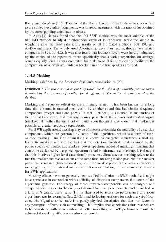
From Physics to Psychophysics 41
Illenyi and Korpassy [116]. They found that the rank order of the loudspeakers, accordingto the subjective quality judgements, was in good agreement with the rank order obtainedby the corresponding calculated loudness.
In Aarts [4], it was found that the ISO 532B method was the most suitable of thetwo ISO methods to adjust interloudness levels of loudspeakers, while the simple B-weighting gave the most satisfactory results of all the tested methods (both ISO andA–D weightings). The widely used A-weighting gave poor results, though (see relatedcomments in Sec. 1.4.4.2). It was also found that loudness levels were hardly influencedby the choice of the repertoire, more specifically that a varied repertoire, on average,sounds equally loud, as was computed for pink noise. This considerably facilitates thecomputation of appropriate loudness levels if multiple loudspeakers are used.
1.4.4.5 Masking
Masking is defined by the American Standards Association as [20]
Definition 7 The process, and amount, by which the threshold of audibility for one soundis raised by the presence of another (masking) sound. The unit customarily used is thedecibel.
Masking and frequency selectivity are intimately related; it has been known for a longtime that a sound is masked most easily by another sound that has similar frequencycomponents (Wegel and Lane [295]). In fact, Fletcher [72] assumed, in his studies ofthe critical bandwidth, that masking is only possible if the masker and masked signal(maskee) fall within the same critical band, even though it was known that masking ispossible at greater frequency separations.
For BWE applications, masking may be of interest to consider the audibility of distortioncomponents, which are generated by some of the algorithms, which is a form of tone-on-tone masking. This kind of masking is known as energetic, simultaneous masking.Energetic masking refers to the fact that the detection threshold is determined by thepower spectra of masker and maskee (power spectrum model of masking); masking thatcannot be explained by the power spectrum model is informational masking. It is thoughtthat this involves higher-level (attentional) processes. Simultaneous masking refers to thefact that masker and maskee occur at the same time; masking is also possible if the maskerprecedes the maskee (forward masking), or if the maskee precedes the masker (backwardmasking). Both informational and non-simultaneous masking do not seem very relevantfor BWE applications.
Masking effects have not generally been studied in relation to BWE methods; it mighthave some use in connection with audibility of distortion components that some of thealgorithms generate. The energy of these unwanted components can be analyzed andcompared with respect to the energy of desired frequency components, and quantified asa kind of ‘signal-to-noise’ ratio. This is then used to assess the performance of variousalgorithms; see for example, Sec. 2.3.2.1, and following sections, for such analysis. How-ever, this ‘signal-to-noise’ ratio is a purely physical description that does not factor inany perceptual effects, such as masking. This implies that conclusions thus reached areto be considered with some caution. A better modelling of BWE performance could beachieved if masking effects were also considered.

42 Audio Bandwidth Extension
1.4.5 PITCH
1.4.5.1 Factors Influencing Pitch
According to the American Standards Association [20] pitch is defined as follows
Definition 8 Pitch: that attribute of an auditory sensation in terms of which sounds maybe ordered on a scale extending from low to high.
According to Moore [177], there are various ways how the pitch of a pure tone depends onits frequency. One can obtain a pitch–frequency relation by various methods, the classicalresult being the mel scale. It has an arbitrary pitch reference of 1000 mel at a frequencyof 1000 Hz. A tone that sounds, on average, twice as high receives a value of 2000 mel,whereas a tone that sounds only half as high has a pitch of 500 mel. Although the melscale suggests that the pitch of a pure tone is simply determined by its frequency, theperceived pitch also depends on some other factors, one of them being the intensity. If onemeasures for a group of subjects how, on average, the pitch of a pure tone changes with thetone’s intensity, one typically finds that (1) for tones below 1000 Hz the pitch decreaseswith increasing intensity (about 15%), (2) for tones between 1000 and 2000 Hz the pitchremains rather constant, and (3) for tones above 2000 Hz the pitch rises with increasingintensity (about 20%). This effect varies considerably between listeners and also dependson the duration of the tone. Hartmann [105] found that the pitch of short-duration tones(≈100 ms) with decaying envelopes is higher than the frequency of the tone. The upwardpitch shift seems to increase with decreasing frequency, being 2.6% at a frequency of412 Hz (the lowest frequency used by Hartmann). The shift at even lower frequenciescould be considerably higher, although there is no data to support this hypothesis.
For a complex tone, consisting of more than one frequency component, the situationis more complicated. Pitch should then be measured by psychophysical experiments. Apitch that is produced by a set of frequency components, rather than by a single sinusoid,is called a residue. Even if in a harmonic complex the fundamental frequency is missing,it will still be perceived as a residue pitch, which in this case is sometimes called virtualpitch, because the frequency corresponding to the pitch is absent. There is a vast literatureon pitch perception and residue pitch. Some of the earlier systematic investigations aredescribed in Bilsen and Ritsma [33], de Boer [58], Houtsma and Goldstein [113], andSchouten [239, 240]). The fact that low-order harmonics need not be physically present toevoke a pitch percept at the fundamental10 is an attractive option to enhance low-pitchedsounds reproduced by (small) loudspeakers; in Chapter 2, we shall see how this can beexploited. One factor that remains unclear is the strength of the residue pitch at verylow frequencies (<100 or 200 Hz); most investigators have looked at higher frequencies.Ritsma [225, 226] has studied the existence region above 200 Hz.
Repetition pitch Some noise-like sounds do evoke pitch sensations. An example wasdescribed by Huygens [115] in the seventeenth century. He noticed that the noise of awater fountain, reflected by marble stairs, produced a distinct musical pitch equal to thatof an organ pipe whose length matched the depth of the stairs. He essentially discovered
10In fact, the residue pitch can be heard even if there is a masking noise present in the frequency region of the
fundamental such that it would normally be masked (Licklider [161]).
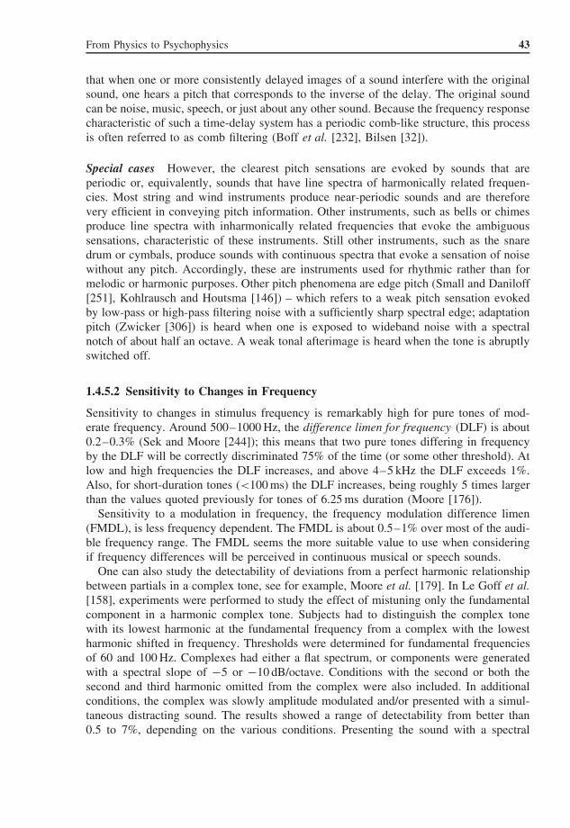
From Physics to Psychophysics 43
that when one or more consistently delayed images of a sound interfere with the originalsound, one hears a pitch that corresponds to the inverse of the delay. The original soundcan be noise, music, speech, or just about any other sound. Because the frequency responsecharacteristic of such a time-delay system has a periodic comb-like structure, this processis often referred to as comb filtering (Boff et al. [232], Bilsen [32]).
Special cases However, the clearest pitch sensations are evoked by sounds that areperiodic or, equivalently, sounds that have line spectra of harmonically related frequen-cies. Most string and wind instruments produce near-periodic sounds and are thereforevery efficient in conveying pitch information. Other instruments, such as bells or chimesproduce line spectra with inharmonically related frequencies that evoke the ambiguoussensations, characteristic of these instruments. Still other instruments, such as the snaredrum or cymbals, produce sounds with continuous spectra that evoke a sensation of noisewithout any pitch. Accordingly, these are instruments used for rhythmic rather than formelodic or harmonic purposes. Other pitch phenomena are edge pitch (Small and Daniloff[251], Kohlrausch and Houtsma [146]) – which refers to a weak pitch sensation evokedby low-pass or high-pass filtering noise with a sufficiently sharp spectral edge; adaptationpitch (Zwicker [306]) is heard when one is exposed to wideband noise with a spectralnotch of about half an octave. A weak tonal afterimage is heard when the tone is abruptlyswitched off.
1.4.5.2 Sensitivity to Changes in Frequency
Sensitivity to changes in stimulus frequency is remarkably high for pure tones of mod-erate frequency. Around 500–1000 Hz, the difference limen for frequency (DLF) is about0.2–0.3% (Sek and Moore [244]); this means that two pure tones differing in frequencyby the DLF will be correctly discriminated 75% of the time (or some other threshold). Atlow and high frequencies the DLF increases, and above 4–5 kHz the DLF exceeds 1%.Also, for short-duration tones (<100 ms) the DLF increases, being roughly 5 times largerthan the values quoted previously for tones of 6.25 ms duration (Moore [176]).
Sensitivity to a modulation in frequency, the frequency modulation difference limen(FMDL), is less frequency dependent. The FMDL is about 0.5–1% over most of the audi-ble frequency range. The FMDL seems the more suitable value to use when consideringif frequency differences will be perceived in continuous musical or speech sounds.
One can also study the detectability of deviations from a perfect harmonic relationshipbetween partials in a complex tone, see for example, Moore et al. [179]. In Le Goff et al.[158], experiments were performed to study the effect of mistuning only the fundamentalcomponent in a harmonic complex tone. Subjects had to distinguish the complex tonewith its lowest harmonic at the fundamental frequency from a complex with the lowestharmonic shifted in frequency. Thresholds were determined for fundamental frequenciesof 60 and 100 Hz. Complexes had either a flat spectrum, or components were generatedwith a spectral slope of −5 or −10 dB/octave. Conditions with the second or both thesecond and third harmonic omitted from the complex were also included. In additionalconditions, the complex was slowly amplitude modulated and/or presented with a simul-taneous distracting sound. The results showed a range of detectability from better than0.5 to 7%, depending on the various conditions. Presenting the sound with a spectral

44 Audio Bandwidth Extension
slope strongly lowers thresholds. Adding a distractor or applying amplitude modulation,both lead to higher thresholds. The aim of this study was to investigate the perceptualconsequences of a special frequency mapping technique, that is used to exploit the highefficiency of a loudspeaker design (trading high efficiency at the resonance frequency fordecreased efficiency at higher frequencies), described in Sec. 4.3. The more complex stim-uli used in the subjective experiment were thought to mimic signals that would typicallybe reproduced through this special driver.
1.4.5.3 Pitch Theories
A number of theories have been developed to explain the pitch of complex tones, whichled to what are now known as the place and periodicity theories of pitch perception.Among these are the early theories of Ohm [190] and Seebeck [243]. Others, includingHelmholtz [108], assumed that if the fundamental frequency of a harmonic stimuluswas absent, non-linear distortion in the middle ear could recreate that fundamental as adifference tone.
Place theories of pitch perception Briefly, the place theory of pitch perception assumesthat the cochlea performs a spectral analysis of the sound and maps different frequencycomponents along the BM (tonotopic organization, see Sec. 1.4.1); then the various loca-tions where spectrally resolved partials are detected are used to derive a pitch percept.This implies that tones without resolved partials have no definite pitch. Several modelsfor such pitch extraction have been put forward, some of which are:
• Closest matching subharmonic of lowest partial (Walliser [293]): The first step is todetermine the stimulus envelope repetition rate; this corresponds to the frequency dif-ference of the partials. Next, a subharmonic of the lowest partial is determined that isclosest to the frequency found in the first step.
• Most frequently occurring subharmonic: Terhardt [266] elaborated upon Walliser’smodel, and assumed that each partial elicits a number of subharmonics that are pitch‘candidates’. For a complex tone, there will be one subharmonic that occurs most fre-quently, which determines the perceived pitch. Ambiguous pitch percepts are possibleif several candidate subharmonics have roughly equal number of occurrences or ifsubharmonics cluster around multiple values.
• Optimum processor (Goldstein [92]): The estimated frequency values of the partials arefed into a kind of pattern recognition device, which first estimates the correspondingharmonic numbers and then derives the best-matching subharmonic to fit the observedpartials; that subharmonic will be the perceived pitch. This model explains ambiguouspitch percepts by assuming that errors can be made in the estimation of harmonicnumber.
It is noted that in all of these models the use of place information is not an absoluterequirement. The frequencies of the partials could be derived through timing information.
These models predict pitch values not only for ‘normal’ complex tones, but also forcomplex tones where each partial is shifted in frequency by a fixed amount, creatingan inharmonic complex that does not have a ‘proper’ fundamental frequency. Although
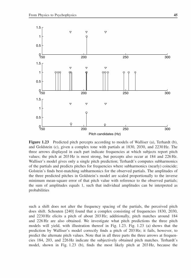
From Physics to Psychophysics 45
150 200 250 3000
0.5
1
1.5
150 200 250 3000
0.5
1
1.5
150 200 250 3000
0.5
1
1.5
Pitch candidates (Hz)
Figure 1.23 Predicted pitch percepts according to models of Walliser (a), Terhardt (b),and Goldstein (c), given a complex tone with partials at 1830, 2030, and 2230 Hz. Thethree arrows displayed in each part indicate frequencies at which subjects report pitchvalues; the pitch at 203 Hz is most strong, but percepts also occur at 184 and 226 Hz.Walliser’s model gives only a single pitch prediction; Terhardt’s computes subharmonicsof the partials and predicts pitches for frequencies where subharmonics (nearly) coincide;Golstein’s finds best-matching subharmonics for the observed partials. The amplitudes ofthe three predicted pitches in Goldstein’s model are scaled proportionally to the inverseminimum mean-square error of that pitch value with reference to the observed partials;the sum of amplitudes equals 1, such that individual amplitudes can be interpreted asprobabilities
such a shift does not alter the frequency spacing of the partials, the perceived pitchdoes shift. Schouten [240] found that a complex consisting of frequencies 1830, 2030,and 2230 Hz elicits a pitch of about 203 Hz; additionally, pitch matches around 184and 226 Hz are also obtained. We investigate what pitch predictions the three pitchmodels will yield, with illustration thereof in Fig. 1.23. Fig. 1.23 (a) shows that theprediction by Walliser’s model correctly finds a pitch of 203 Hz; it fails, however, topredict the alternate pitch values. Note that in all three parts the three arrows at frequen-cies 184, 203, and 226 Hz indicate the subjectively obtained pitch matches. Terhardt’smodel, shown in Fig. 1.23 (b), finds the most likely pitch at 203 Hz, because the
46 Audio Bandwidth Extension
subharmonics cluster most closely around that value. Pitch matches at 184 and 226 Hzare also correctly obtained, but with less likelihood, as the clustering is not as tightaround these values. Fig. 1.23 (c) shows predictions from Goldstein’s model. In thiscase, the amplitudes of the pitch matches indicate the probability of subjectively find-ing that particular pitch on any given occasion. For this, we have used an ad hoc metricthat relates the probability of a pitch match to the inverse of the minimum mean-squareerror for that pitch match, given the observed harmonics. Goldstein’s model also cor-rectly matches the 203-Hz pitch, by assuming the harmonic numbers to be 9, 10, and11; if the harmonic numbers are overestimated by 1, the pitch match at 184 Hz is pre-dicted, and if the harmonic numbers are underestimated by 1, the pitch match at 226 Hzis predicted. Note that the pitch ambiguity that is observed in this example is primarilydue to the absence of lower harmonics, which, if present, would give far less ambiguouspredictions in either Terhardt’s or Goldtein’s model. This is also subjectively observed,and, in fact, it is believed that low-order harmonics (number ≈3–6) are dominant withrespect to pitch determination, even if the fundamental is physically present (Plomp [209],Ritsma [227]).
Periodicity theories of pitch perception In the periodicity, or temporal, theory the loca-tions of the BM that are excited are not important (although the tonotopic organizationof the cochlea per se is not disputed); rather, periodicities in neural activity are used toderive pitch information. Periodicities in neural activity are caused by the fact that neu-ral response occurs preferentially during a specific phase of the BMM waveform (phaselocking). The original temporal theory is mainly due to Schouten [239], who devisedan ingenious theory that combined peripheral frequency analysis and central periodicitydetection. According to his theory, the lower components of a harmonic complex arespectrally resolved in the cochlea (see Sec. 1.4.3) and each map into their own pitch.The higher components, which are not resolved, create a periodic interference pattern thatreflects the periodicity of the waveform. This periodicity is detected by higher neural cen-ters and maps into a sensation of (fundamental) pitch. This gave rise to the term residuepitch, because, according to Schouten, it results from the residue of spectral componentsthat the cochlea fails to resolve (Boff et al. [232]). The actual pitch that is assigned to thesound is that pitch to which attention is mainly drawn; for complex tones this is generallythe residue pitch. Note that the temporal theory can also account for ambiguous pitch ofinharmonically related partials, as in the example of Fig. 1.23.
Numerous experiments have shown support for both theories. It appears that neithertheory alone can account for all conditions, and as such it seems likely that both placeand timing information can and are used for pitch perception. Moore [177] presents aqualitative model that incorporates both place and timing information and can accountfor all experimental data.
1.4.6 TIMBRE
Timbre is defined by the American Standards Association [20] as follows.
Definition 9 Timbre: that attribute of an auditory sensation in terms of which a listenercan judge that two sounds similarly presented and having the same loudness and pitch aredissimilar.
From Physics to Psychophysics 47
This is, as has also been noted by others, a better description of what timbre is not thanwhat it is. It is problematic to define exactly what timbre is because it does not appear to bea one-dimensional quantity. Timbre is known to depend on short-term power spectrum (ormore properly, the excitation pattern), amplitude envelope (in particular, attack and decaytime), and phase spectrum. Plomp and Steeneken [210] carried out a clever experimentto investigate the relative influence of power spectrum versus phase spectrum on timbre.They used signals s(t) of the form
s(t) =N∑
n=1
an sin(2πf0t) + bn cos(2πf0t), (1.94)
and found (using triadic comparisons and multidimensional scaling) that the largest timbraldifference occurred between signals where all an (or bn) were zero and signals where thean and bn were alternately zero. They proceeded to investigate what changes in powerspectrum would yield the same magnitude of timbral difference as was found for thephase effect. The an and bn were chosen to decay by a fixed amount in dB per octave,varied between −4.5 and −7.5 dB, in 0.5-dB steps. The maximum influence of phasespectrum as discussed above could be matched by a change in the power spectrum slopeof 2 dB, at f0 = 146.2 Hz. The influence of phase spectrum decreases for increasingf0, being matched by a 0.7-dB change in the power spectrum slope for f0 = 584.4 Hz.Also, it appeared that phase spectrum and power spectrum influences were independentof one another. In conclusion, this experiment showed that phase spectrum does influencetimbre, but less so than the power spectrum. In practice, when listening to signals overloudspeakers, the relative phases of frequency components become randomized because ofroom reflections, which means that the signal’s original phase spectrum will be modified.It thus appears that it is not practical to try to control the phase spectrum, unless listeningoccurs via headphones. In BWE algorithms, timbre can thus be adjusted by modifyingharmonic amplitudes, for example, through filtering.
Timbre of a sound is usually qualitatively described using several descriptors. Onesuch descriptor that seems to be well linked to an objective parameter of the signal is‘brightness’; it is related to the relative amount of high frequencies versus low frequenciescontained in the signal. Brightness can be quantatively described by the spectral centroidCS , or power spectral center of gravity, as
CS =∫
f 10 log S2(f ) df∫10 log S2(f ) df
, (1.95)
given a signal with power spectrum11 S2(f ). If, for example,, the relative amplitudesof the harmonics of a complex tone are modified (as most of the BWE algorithms do),CS will change, while the pitch remains the same. Equation 1.95 is only a first-orderapproximation of what the spectral centre of gravity is for the internal representation of
11It is more proper to use a compressed power spectrum (e.g. by taking the cube root), which corresponds better
to the BMM. For simplicity, we keep using S(f ) in the remainder of the book. It should be noted that if spectralcentroid is quantatively used for analysis purposes, a perceptually much more accurate version must be employed.
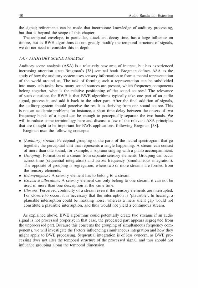
48 Audio Bandwidth Extension
the signal; refinements can be made that incorporate knowledge of auditory processing,but that is beyond the scope of this chapter.
The temporal envelope, in particular, attack and decay time, has a large influence ontimbre, but as BWE algorithms do not greatly modify the temporal structure of signals,we do not need to consider this in depth.
1.4.7 AUDITORY SCENE ANALYSIS
Auditory scene analysis (ASA) is a relatively new area of interest, but has experiencedincreasing attention since Bregman’s [38] seminal book. Bregman defines ASA as thestudy of how the auditory system uses sensory information to form a mental representationof the world around us. The task of forming such a representation can be subdividedinto many sub-tasks: how many sound sources are present, which frequency componentsbelong together, what is the relative positioning of the sound sources? The relevanceof such questions for BWE is that BWE algorithms typically take one part of an audiosignal, process it, and add it back to the other part. After the final addition of signals,the auditory system should perceive the result as deriving from one sound source. Thisis not an academic problem; for instance, a short time delay between the onsets of twofrequency bands of a signal can be enough to perceptually separate the two bands. Wewill introduce some terminology here and discuss a few of the relevant ASA principlesthat are thought to be important for BWE applications, following Bregman [38].
Bregman uses the following concepts:
• (Auditory) stream: Perceptual grouping of the parts of the neural spectrogram that gotogether; the perceptual unit that represents a single happening. A stream can consistof more than one sound, for example, a soprano singing with a piano accompaniment.
• Grouping : Formation of a stream from separate sensory elements. Grouping can occuracross time (sequential integration) and across frequency (simultaneous integration).The opposite of grouping is segregation, where two or more streams are formed fromthe sensory elements.
• Belongingness: A sensory element has to belong to a stream.• Exclusive allocation: A sensory element can only belong to one stream; it can not be
used in more than one description at the same time.• Closure: Perceived continuity of a stream even if the sensory elements are interrupted.
For closure to occur, it is necessary that the interruption is ‘plausible’. In hearing, aplausible interruption could be masking noise, whereas a mere silent gap would notconstitute a plausible interruption, and thus would not yield a continuous stream.
As explained above, BWE algorithms could potentially create two streams if an audiosignal is not processed properly; in that case, the processed part appears segregated fromthe unprocessed part. Because this concerns the grouping of simultaneous frequency com-ponents, we will investigate the factors influencing simultaneous integration and how theymight apply to BWE processing. Sequential integration is of less concern, as BWE pro-cessing does not alter the temporal structure of the processed signal, and thus should notinfluence grouping along the temporal dimension.

From Physics to Psychophysics 49
Factors influencing simultaneous integration are:
• Correspondence over time: If a complex spectrum consists, in part, of a simpler spec-trum that was present previously, the simple spectrum would appear to continue. The‘difference’ spectrum would appear as a new tone (‘old-plus-new’ heuristic).
• Harmonicity : Components with a harmonic frequency relationship are grouped, andassigned a fundamental pitch.
• Common fate: Components that have correlated changes in frequency (frequency modu-lation, FM) or amplitude (amplitude modulation, AM) are grouped. Naturally producedspeech and music sounds often exhibit micromodulation (slight modulations on smalltime scales) as well as modulations on a larger time scale. An extreme example ofamplitude modulation is an onset or offset. The common AM during an onset is anespecially strong grouping cue.
• Spatial direction: Components arriving from the same direction are grouped; in con-trast, components arriving from different directions are segregated. This cue can bequite strong, although it can be acoustically ambiguous, which is why it breaks downeasily if in conflict with any of the other factors mentioned earlier.
The tendency for simultaneous frequency components to group depends on how manyof the factors mentioned here favor grouping versus segregation. The various factorsreinforce each other, and grouping (or segregation) will be strongest if many or all of thefactors are in ‘agreement’.
For BWE applications, harmonicity and common fate principles seem of greatest impor-tance. Music and speech signals abound with harmonic signals (although noise-like sig-nals also occur), and this harmonic structure should be maintained as much as possible.Some of the BWE algorithms actively produce harmonics of input signal components,which promotes grouping. Because the production of harmonics occurs through non-linearprocessing, inharmonic (distortion) components can, in some cases, also be generated.Depending on the relative energy of harmonic versus distortion products, the distortionwill be audible. The distortion will covary in amplitude with the harmonic components,and may therefore be grouped into the same stream. Of course, perceptible distortionshould be avoided as much as possible, regardless of grouping or segregation. Anotherimportant result is that the processed signals should not be excessively delayed withrespect to the unprocessed signal: the common fate principle implies that the delayedonset of the processed signal could segregate it from the unprocessed signal. Zera andGreen [304] found that in some cases, delays on the order of milliseconds can lead todiscriminable changes in perception (though this does not necessarily imply segregation).This will be discussed in more detail in Sec. 2.3.3.3, and solutions will be given to avoidsuch potential problems.
1.4.8 PERCEPTUAL MODELLING – AUDITORY IMAGE MODEL
The auditory image model (AIM) can be used to visualize internal representations (‘audi-tory images’) of sounds, and is described elaborately in Patterson et al. [203, 202]. Bothfunctional and physiological modules can be selected that model the use of fine-grain
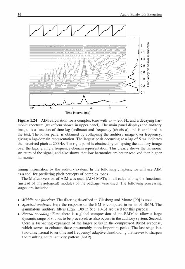
50 Audio Bandwidth Extension
12481632
Time interval (ms)
0.1
0.2
0.3
0.6
0.9
1.4
2.1
3
Fre
quen
cy o
n ba
sila
r m
embr
ane
Figure 1.24 AIM calculation for a complex tone with f0 = 200 Hz and a decaying har-monic spectrum (waveform shown in upper panel). The main panel displays the auditoryimage, as a function of time lag (ordinate) and frequency (abscissa), and is explained inthe text. The lower panel is obtained by collapsing the auditory image over frequency,giving a lag-domain representation. The largest peak occurring at a lag of 5 ms indicatesthe perceived pitch at 200 Hz. The right panel is obtained by collapsing the auditory imageover the lags, giving a frequency-domain representation. This clearly shows the harmonicstructure of the signal, and also shows that low harmonics are better resolved than higherharmonics
timing information by the auditory system. In the following chapters, we will use AIMas a tool for predicting pitch percepts of complex tones.
The MatLab version of AIM was used (AIM-MAT); in all calculations, the functional(instead of physiological) modules of the package were used. The following processingstages are included:
• Middle ear filtering : The filtering described in Glasberg and Moore [90] is used.• Spectral analysis: Here the response on the BM is computed in terms of BMM. The
gammatone auditory filters (Eqn. 1.89 in Sec. 1.4.3) are used for this purpose.• Neural encoding : First, there is a global compression of the BMM to allow a large
dynamic range of sounds to be processed, as also occurs in the auditory system. Second,there is fast-acting expansion of the larger peaks in the compressed BMM response,which serves to enhance these presumably more important peaks. The last stage is atwo-dimensional (over time and frequency) adaptive thresholding that serves to sharpenthe resulting neural activity pattern (NAP).

From Physics to Psychophysics 51
• Time-interval stabilization: Because periodic sounds give rise to static, rather thanoscillating, percepts, it is assumed that a temporal integration is performed on theNAP. To preserve the fine structure present in the timing of the NAP, a so-called‘strobed’ temporal integration occurs. The integration commences when a peak in theNAP is encountered, after which the NAP input to the integrator decays in time.
The result of these processing steps is the auditory image, an example of which is shownin Fig. 1.24, where a complex tone with a 200-Hz fundamental was used. The auditoryimage can be collapsed over the time lags, to obtain an internal spectral representationof the signal (right panel of Fig. 1.24). Alternatively, a collapse over frequency providesa temporal representation of the signal (lower panel). Owing to the nature of the strobedtemporal integration, this temporal representation is interpreted as a lag with respect tothe last strobe: repetitions in the NAP show up as peaks in the auditory image at theappropriate lag values. Therefore, a signal with a temporal periodicity will exhibit peaksin the auditory image, which occur at a lag value equal to the periodicity interval; therebypredicting a pitch percept for the given signal at a frequency, which is the inverse of thelag. In Fig. 1.24, we find that the largest peak in the lag domain occurs at 5 ms, as wewould expect on the basis of the 200-Hz fundamental frequency. We interpret the pitchstrength as corresponding to the width of the peak, with wider peaks corresponding to theweaker pitch. If multiple peaks occur, the likelihood of pitch matches corresponds to therelative height of peaks. On the other hand, multiple peaks could indicate that the givensignal segregates into two (or more) streams, each with their own pitch. As AIM doesnot incorporate auditory scene analysis principles, it does not predict which of these twopossibilities applies to the given signal.
